NON-LINEAR EFFECTS IN ELECTROMAGNETIC WAVE ACTIVITY

OBSERVED IN THE RELEC EXPERIMENT ON-BOARD VERNOV MISSION

M.I. Panasyuk

1,2, S.I. Svertilov

1,2, S.I. Klimov

3, V.A. Grushin

3, D.I. Novikov

3, S.P. Savin

3,

Yu.Ya. Ruzhin4, Yu.M. Mikhailov

4, Cs. Ferencz

6, P. Szegedi

7, V.E. Korepanov

5,

V.V. Bogomolov1,2

, G.K. Garipov1, S.V. Belyaev

5, A.N. Demidov

5

1 –Lomonosov Moscow State University, D.V. Skobeltsyn Institute of Nuclear Physics

2 –Lomonosov Moscow State University, Physics Department 3 – Space Research Institute, Russian Academy of Sciences, Moscow, Russia

4 –Pushkov Institute of the Earth magnetism, Ionosphere and radio-wave propagation, Russian Academy of

Sciences, Troitsk, Russia 5 – Institute of Space Research, Ukrainian Academy of Sciences and National Space Agency, Lviv, Ukraina

6 – Eötvös University, Space Research Group, Budapest, Hungary 7- BL Electronics Ltd., Solymár, Hungary

The experiments on-board Vernov satellite were aimed on the study of high energy (relativistic and sub-

relativistic) electron acceleration and losses in the trapped radiation areas as well as high altitude electric

discharges in the upper Atmosphere. A separate task was study electromagnetic-wave phenomena in the

near Earth space and the upper Atmosphere. During observations on December 10, 2014 interesting

phenomena were discovered. They are connected to non-linear effects in wave activity of the type of two

or three wave decays as well as splitting into two wave structures. Whistlers with specific unusual

temporal structure which looked like a high frequency tail rising were observed on the spectral diagrams

(sonograms), which were obtained for this time. It was shown that such signals can be caused by seismic

activity. The signals of the type of whistler with long tail were also observed. Such signals were also

detected by ground stations.

1. Introduction. The aim of scientific experiments with RELEC (acronym Relativistic ELECtrons)

instruments on-board Vernov satellite (Panasyuk et al., 2016a) was complex study of processes

with high energy electrons in the near Earth space, ionosphere and upper Atmosphere including

magnetosphere electron precipitation and transient electromagnetic events in the Earth

Atmosphere caused by high-altitude atmospheric discharges. Of-coarse these phenomena are

tightly connected with wide frequency electromagnetic (EM) waves. Some natural EM

phenomena known as space whether and occur in the solar wind – magnetosphere – ionosphere –

Earth Atmosphere system generate electromagnetic waves that can be detected in the ionosphere.

Whistlers generated by thunderstorm discharges and detected by satellites are typical example of

such emissions. Thus, study of EM environment in the near Earth space was also among the

main tasks of the RELEC experiment.

It is well-known, that precipitations in the loss cone occur as a result of a change in the

pitch-angle distribution of the particles mainly due to wave-particle interaction (see e.g. Lyons,

et al., 1972). Calculation of the corresponding electron loss rates requires information about the

spectra of the excited waves. Several wave modes generated and propagated in the

magnetosphere can interact with relativistic electrons. Among them are whistlers, whistler-mode

waves, EM ion cyclotron and electrostatic ion cyclotron waves. The waves are often generated

by particles of lower energies, these waves then precipitate particles of higher energies (parasitic

diffusion).

Whistler mode waves and electrostatic ion-cyclotron waves scatter most effectively

electrons with energies <1 MeV, but they also can scatter particles with higher energies (see e.g.

Gurevich, 2007). Electromagnetic ion-cyclotron waves scatter electrons with energies >1 MeV

more effectively. Precipitation in the loss cone is connected usually with gyro-resonance

interaction of particles with whistler-mode waves, electromagnetic ion-cyclotron (EMIC) waves

and plasmaspheric hisses. This problem was studied in details, see e.g. Kennel and Petscheck,

1966; Horne and Thorne, 2003; Thorne et al., 1977; Summers and Thorne, 2003; Albert, 2003;

Meredith et al., 2006; Shprits et al., 2008 a,b and Ferencz et al., 2001.

Atmospherics or spherics are electromagnetic signals produced by lightning discharges

(see e.g. Roussel‐ Dupré, et al., 2008.). The average occurrence of lightnings is about 100 strikes

per second. A lightning discharge consists of two stages. There are pre-discharges and main

discharges, which differ by current and spectrum of emitted radio-waves. Ultra-long waves are

emitted in the main discharge, while long, middle and even short waves are emitted in the pre-

discharge.

The maximum of spheric energy lies in the range of about 4-8 kHz (see e.g. Ferencz, et

al. 2010.). If spherics are produced by nearby thunderstorms, their spectrum is determined only

by the emission spectrum of thunderstorm discharge. If the source is a distant thunderstorm, its

spectrum is determined also by the conditions of radio-wave propagation from the thunderstorm

to the radio receiver. Spherics have a weak attenuation and can propagate over long distances.

Spherics may penetrate into the ionosphere and propagate along the magnetic field line,

reaching the Earth-Ionosphere waveguide again in the other hemisphere and can be recorded on

the ground. These waves exhibit frequency changes versus time and called whistlers. Their

peculiarity is associated with Very Low Frequency wave propagation in magneto-ionic medium,

see e.g. Hellivell, 1965; Ferencz et al. 2007, 2009; Ferencz et al., 2001.

The type of spheric spectrum is determined by magnetic field intensity and electron

concentration along trajectory. The spectrum covers frequencies from hundreds Hz up to 20-30

kHz (Klimov et al., 2014). The spheric property analysis allows us to determine the electron

concentration distribution along the propagation path, see e.g. Park, 1972; Lichtenberger, 2009.

A rare phenomenon called knee whistlers (Carpenter, 1963) may be used to determine the

location of the plasmapause. Low-frequency branches of the spheric spectrum (ion whistlers)

were detected on the satellites at frequencies below 400-500 Hz, over which the relative

concentrations of ions and electrons, as well as other parameters of the ionosphere can be

determined.

ULF-ELF-VLF electromagnetic radiation plays the same role for the study of plasma

processes in space as seismic waves for the Earth structure study. In comparison with EM

processes in other environments, waves in plasma have a number of definite characteristic

peculiarities. The resonance effect is the most important. It occurs due to the wave-particle

interaction, wave transformations, resonator and waveguide formation. Due to the resonance

effect, ultra-low frequency waves provide information about dynamic phenomena in the near-

Earth space and the upper Atmosphere. By this they reach sufficiently large amplitudes to have

significant influence on the plasma fluxes and effectively accelerate electrons in the

magnetosphere. It was shown recently, that not only magnetosphere – ionosphere phenomena are

accompanied by plasma disturbance, but also ground geophysical ones caused by large energy

release such as explosions, hurricanes, thunderstorms and earthquakes.

Emission intensity increasing in the ELF-VLF bands observed before earthquakes on

many satellites in the narrow-band detection mode. However, to the present time, the nature of

this effect remains controversial. Our cycle of work using broadband and narrowband

observations on board satellites has allowed us to obtain previously unknown data on this effect.

Thus, the first detection of broadband ELF-VLF emissions were performed on the satellite

Intercosmos-24 during its fly for three hours over the area of the Iranian earthquake since the

beginning of the June, 20 at 21:00:07,1 UT (Mikhailov et al., 1991). The observed nature of the

emission was not noise, as indicated in other studies, but discrete with the parameters of typical

partially dispersed whistler. It was discovered that their follow-up frequency was abnormally

high and intensity was higher in comparison with usually rarely observed signals in morning

hours of local time at similar heights and latitudes. Also the big extent on latitude of their

detection zone was found.

The other intriguing problem is study of non-linear phenomena in EM environment. Due

to the exponentially rapid change in the concentration of neutral molecules with height in the

Atmosphere and the presence of the Earth’s magnetic field, the properties of a free ionospheric

plasma are extremely diverse. A large number of different waves can exist in a plasma in a

magnetic field, which causes an extremely large variety of nonlinear phenomena in the

ionospheric plasma (Gurevich, et al. 2007). In the case of weak nonlinearity, the main nonlinear

wave process in plasma is three-wave resonance, for which the conservation laws describing

such processes must be satisfied, i.e. one wave splits into two waves, two waves merge into one

wave. The references also one can find in (Savin, et al, 2014).

Interesting EM wave phenomena possible connected with seismic activity and non-linear

processes were observed during the RELEC Vernov experiment on December 10, 2014. Detailed

analysis of these events will be presented below in subsequent sections of this article.

2. Magnetic-wave instruments PSA – RFA as a part of the RELEC scientific

payload on-board Vernov satellite. The RELEC scientific payload described in details by Panasyuk et al., 2016 b,c was

operated on-board small spacecraft Vernov between July – December, 2014. It was named in

honor of pioneer of space research Soviet academician Sergey Nikolaevich Vernov. The satellite

orbit was sun -synchronous with apogee 830 km, perigee 640 km, inclination 98.4о and orbital

period 100 min.

The EM emission and current in plasma in wide frequency range were measured by

NChA – RChA (PSA – RFA) complex. These instruments allowed high accuracy measurements

of values and fine structure of field variations.

The NChA – RChA (PSA, i.e.SAS3-R – RFA) complex of instruments consisted from

the low frequency analyzer NChA (PSA – SAS3-R) and the radio frequency analyzer RChA

(RFA).

The NChA (PSA – SAS3-R) instrument consisted of the following units:

- data processing unit for spectral analysis PSA;

- flux gate magnetometer, detector unit (DFM) and electronic unit (BE-FM);

- induction magnetometer IM;

- two identical complex wave probe (CWZ-1, CWZ-2).

The RChA (RFA) instrument consited of an analyzer unit RFA-E and three-component

electric antenna RFA-AE.

The NChA – RChA units were mounted on the outer 3 meters boom (IM, DFM, CWZ-1,

CWZ-2, RFA-AE) and on the spacecraft thermostatic panel (units BE-FM, PSA, RFA-E). Their

sizes, masses and power consumption are presented in Panasyuk et al., 2016a.

The sketch of mutual displacement of NChA at the boom is presented in Fig. 1. This

instrument measured the constant magnetic field by a three-component flux gate magnetometer.

The range of measured intensity was no less than ± 64000 nT, non-orthogonality of the meter

component was less than 1º, the sampling frequency was 250 Hz. The mutual orthogonality of

three measuring axes was provided by the DFM construction

Measurements of values and sign of three components of variable magnetic field

induction vector were made with the use of the induction magnetometer IM and magnetic

channels of the complex wave probes CWZ-1, CWZ-2. Each of these instruments contained one-

component meter of variable magnetic field. To construct an orthogonal coordinate system

mutual orthogonality of Z axes of these instruments was provided. The frequency range of the

meter was from 0.1 to 40000 Hz.

Measurements of plasma current density were made by current measurement channels of

the CVZ-1, CVZ-2 probes. In order to obtain correct results of measurements these probes were

mounted in such a way, that their YOZ planes were parallel to the spacecraft velocity vector.

Fig. 1. Mutual orientation of PSA – SAS3-R sensors. Xsc, Ysc, Zsc – axes of the spacecraft; Vsc

- velocity vector of the spacecraft; Ycwz1, Zcwz1 - measuring axes of the CWZ1; Ycwz2, Zcwz2

- measuring axes of the CWZ2.

Measurements of the potential difference were made with the use of electric channels of

the CWZ-1, CWZ-2 probes, each contained the meter of potential relative the common wire.

The difference of analogue signals from CWZ-1, CWZ-2 was determined in the PSA

unit. The signal from CWZ-1 relative to the common wire was also measured there. The

common wire was connected with spacecraft via telemetry unit, i.e. via high resistor. Thus the

potential difference between CWZ—1 place and spacecraft was determined.

The PSA unit provided:

- producing from the on-board power network 27 V of voltage necessary to its own

operation as well as of the FM, IM, CWZ-1, CWZ-2 operation, that provided its galvanic

isolation from secondary circuits;

- transmission in the digital format of FM, IM, CWZ-1, CWZ-2 outputs;

- calculation of spectral density of measurements values;

- detection of the events, i.e. unusual rare electromagnetic phenomena;

- storing measured data before and after the event;

- storage of measurement results;

- transmission of measurement results and telemetry data to the ground via spacecraft

board systems.

The NChA (PSA – SAS3-R) instrument operated in three main operation modes and a

command controlled recording frequency bandwidth. The main operation modes were the event

detection mode, the monitoring mode and the continuous wave recording (burst) form mode

(means digitization frequency 80 kHz). The recording frequency bandwidth was from <0.1 Hz to

40 kHz. This is approximately two times wider than the frequency bandwidth of the most part of

earlier ionosphere satellite experiments, except the CHIBIS-M micro-satellite electromagnetic

wave measurements, which has also similar up to 40 kHz wide band VLF recording possibilities

(Zeleniy et al., 2014).

The RFA instrument measured high frequency emission. It consisted of an analyzer unit,

RFA-E and antenna, RFA-AE, which was used to measure three electric components of the

electromagnetic field. Physical and technical parameters of RFA instrument units are presented

in Panasyuk et al., 2016a.

The RFA instrument measured three components of electric field, digitized and analyzed

the signals in the band from 50 kHz to 15 MHz. Frequency resolution was 10 kHz, temporal

resolution was 25 ns. The compressed data were transferred to the spacecraft telemetry system.

The wave form digitization unit contained three 12-bit ADC channels. Each analogue

channels included a balancing amplifier with signal shift voltage for balancing the levels with

ADC inputs. The digitized signals were stored in an internal buffer. Then the data were

processed and compressed by the digital signal processor. Depending on the operational mode

and accepted algorithm, there were different types of output signals, such as, wave forms,

compressed wave forms, separate wave numbers or the complete spectrum, compressed number

of spectra (spectral modes). Calculations were made on FPGA according to the programmed

operational modes. The internal memory used either a cyclic buffer or a single-pass FIFO,

depending on the operational mode.

3. Observation of electromagnetic wave activity on 10.12.2014. Interesting events in magnetic wave background occurred on December, 10 at 8:54:57

UT, were recorded in the magnetic Bx channel of NChA (PSA – SAS3-R) instrument, which

operated on December 2014, 10 between 08:54:50.0 - 08:57:10.3 UTC (140 s) in wave recording

form mode in the frequency band 0.1 – 39062.5 Hz of СН0 (Е electric field intensity) and СН3

(Вх-component of magnetic field intensity) channels.

The footprint of the Vernov satellite orbit at the above mentioned time interval is

presented in Fig. 2.

Fig. 2. The Vernov satellite orbit, 10 December 2014, altitude ~ 670 km, local time ~

21:10 LT, magnetic latitude ~ 750.

A sequence of unusual events was revealed on the spectral diagrams (sonograms), which

were obtained for this time. It can be well traced at Вx dynamic spectrograms obtained, which

are presented in Fig. 3. The whistler with specific temporal structure can be seen in the left

panel. This whistler accompanied by non-linear process in wave activity, when initial EM wave

with given frequency underwent decay on two or three wave modes and then two wave

structures occurred. Particular attention should be paid to the emission with increasing

frequency, which was centered at ~ 5 kHz. It is presented in the right panel of Fig. 3.

Fig. 3. The NChA instrument. Spectrograms of Вх on December 10, 2014.

The detailed time structure of the whistler can be analyzed from spectrograms obtained in

wave recording mode for electric field (E) and one magnetic field component (Вx) are presented

in Fig. 3. It is noteworthy that a specific rare emission is seen at 08:54:57 UT, which looked like

a high frequency tail rising from about 10 to 15 kHz. Previously similar structures were also

detected on the Chibis-M microsatellite and named as a “swallow tail” whistler, i.e. STW

(Ferencz et al., 2010; Klimov et al., 2014).

Fig. 4а. Wave form of whistlers detected on E. Fig. 4b. Wave form of whistlers detected on Вх.

The dynamic spectrogram of Е signal for a longer time interval 08:54:50 – 08:57:10 UT

is presented in Fig. 5. There are could be seen three sloping lines as if coming out of one point in

upper left corner of the panel at about 20 kHz. Then these lines diverge by to ~18, ~15 and ~11

kHz. The possible interpretation of such spectral evolution may be three-wave decay from ~ 20

to ~ 18, ~ 15 and 11 kHz. After that two clear structures at 08:56:20 UT are formed.

Fig. 5. Dynamic spectrogram of the event Е signal.

The spectrogram stretched in time is presented in Fig. 6. It confirms the presence of two

structures with size ~30 km, whereas band 15 – 17 kHz as narrow-band ~13 kHz emissions in Е

are observed.

Fig. 6. The same spectrogram as in Fig.5 (Е signal), stretched in time.

The three band-pass frequencies, which can reflect two- or may be three-wave decay

from ~ 20 to ~ 18, ~ 15 and 11 kHz are also presented in the average spectrum of Е signal, which

is shown in Fig. 7.

Fig. 7. The Е field spectrum averaged for 08:54:50.0 - 08:57:10.3 UTC interval.

The wave forms of Е and Вх signals are presented in Fig. 8. The wave form of Е field

exhibits EMC noise with 1 Hz frequency, which due to the wide dynamic range on signal

amplitude (~120 dB) does not lead to the off-scaling of signal. In the Вх signal such noise was

not observed clearly, probably as a result of the sensitivity differences of the sensors.

Fig. 8. The wave forms of Е and Вх signals, left panel corresponds to the – Е field, right panel

corresponds to the Вх field. The time scales are UTC - 3 h.

Quite dramatic transformation of Е frequencies are observed at the end of span ~08:56:50

– 08:57:05 UT, where the emission transferring from frequency ~ 13 kHz to ~ 6 kHz took place

(see Fig. 9).

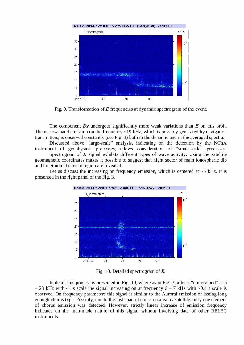
Fig. 9. Transformation of Е frequencies at dynamic spectrogram of the event.

The component Вх undergoes significantly more weak variations than Е on this orbit.

The narrow-band emission on the frequency ~19 kHz, which is possibly generated by navigation

transmitters, is observed constantly (see Fig. 3) both in the dynamic and in the averaged spectra.

Discussed above “large-scale” analysis, indicating on the detection by the NChA

instrument of geophysical processes, allows consideration of “small-scale” processes.

Spectrogram of Е signal exhibits different types of wave activity. Using the satellite

geomagnetic coordinates makes it possible to suggest that night sector of main ionospheric dip

and longitudinal current region are revealed.

Let us discuss the increasing on frequency emission, which is centered at ~5 kHz. It is

presented in the right panel of the Fig. 3.

Fig. 10. Detailed spectrogram of Е.

In detail this process is presented in Fig. 10, where as in Fig. 3, after a “noise cloud” at 6

– 23 kHz with ~1 s scale the signal increasing on at frequency 6 – 7 kHz with ~0.4 s scale is

observed. On frequency parameters this signal is similar to the Auroral emission of lasting long

enough chorus type. Possibly, due to the fast span of emission area by satellite, only one element

of chorus emission was detected. However, strictly linear increase of emission frequency

indicates on the man-made nature of this signal without involving data of other RELEC

instruments.

4. Discussion. The most interesting event was observed on December 10, 2014 at 8:54:57 UT. The

spectrogram of phenomenon presented in Fig. 4 includes two elements. The first is the signal of

increasing frequency in the range 9 – 18 kHz, which similar to the separate chorus element. The

second is whistler itself. Duration of the first element is 0.2 s, rate of frequency changing df/dt =

25 kHz/s. The signal intensity according to the calibration scale presented at the right side of the

figure is about 10–½

µV/m Hz1/2

at 10 kHz frequency. As it was noted by Helliwell, 1965, such

signals are observed multi studiously at the wave intensity В ≈ 310-3

nT/Hz1/2

.

The origin of such signals according to Trachtengerts and Rycroft, 2011 corresponds to

the exiting of trigger signals when energetic electrons occur in the cold plasma region (separate

plasma cloud) during the process of its longitudinal drift. After that the cyclotron instability

mode is switched-on. This signal can be considered presumably as a precursor of a consequent

whistler.

The whistler was analyzed assuming one hop and longitudinal propagation with the

method described in Lichtenberger, 2009, Ferencz et al, 2001. The following parameters were

obtained: L = 2.57, Neq = 2064/ccm, D0 = 66.4, fn = 18544 kHz, fheq = 51234kHz. It was assumed

foF2 = 6 MHz. Here L-shell is the McIllwine parameter of geomagnetic field line; Neq is the

electron concentration at the equatorial area of L-shell; fheq is the hyro-frequency of electrons at

the equatorial area of L-shell; foF2 is the plasma frequency of F2 layer of ionosphere; D0 is the

whistler dispersion; fn is the nose frequency of whistler.

The causative spheric time is 6.36 s from the beginning of the data. The residuals were

average (ms), thus it confirms the inversion. It has to be noted that in the case of a low altitude

recordings, like SAS3 data on the Vernov, it is almost impossible to determine the real

propagation path of the recorded whistler as if it propagated in a duct, it might well left it above

the satellite.

A high-frequency tail at the event (see Fig. 4) reaching 25 kHz indicates the presence of a

low conductivity area at the lower ionosphere in the zone of lightning discharges, which

contributes to the attenuation of the VLF wave absorption. So, by means of statistical processing

Mikhailov et al., 1997a showed that the growth of high-frequency atmospheric penetration is

realized in the region of earthquake before it (see Fig.11 and more detailed comments below).

The expansion of the atmospheric spectrum to higher frequencies, according to the theory of the

properties of the ELF-VLF electromagnetic wave transmission coefficients in the outer

ionosphere, indicates a decrease in the conductivity of the lower ionosphere.

Fig. 11. Histogram of partially dispersed whistler spectra observed on the satellite Intercosmos

24. Dashed line corresponds to the geomagnetic and seismic quiet time, thick line corresponds to

the geomagnetic disturbances, thin line corresponds to the seismic activity in quiet geomagnetic

conditions. The arrow marks the increasing of number of sonograms with frequencies higher

than ~5 kHz.

During the seismically active period in the preparatory phase of earthquakes a shift in the

upper frequency cutoff of the ELF component to higher frequencies and the appearance of the

VLF component is observed in the spectra of whistling atmospherics, i.e. attenuation of the ELF-

and VLF-wave decay at their passing into the outer ionosphere from the Earth-ionosphere

waveguide takes place.

On the other hand, the presence of thunderstorm activity for a few days or hours before

the earthquakes is well known from publications, for example, for the Mediterranean Sea

(Ruzhin et al., 2000; Ruzhin et al., 2007) and for the Kamchatka region (Druzhin, 2002). Thus,

in the last paper, variations in the noise of natural electromagnetic VLF radiation for the period

from January 1997 to December 2001 are considered. It is shown that in Kamchatka a few days

before a strong earthquake, high-power pulsed VLF emissions appear in the noise component,

which usually cease in a few hours or units of day before the main shock. The experience of the

forecast has shown that the anomalous phenomena arising in the noise component of the VLF

signal can be used for the purposes of a short-term forecast of strong earthquakes.

Sorokin et al., 2011; Sorokin et al., 2012; Sorokin and Ruzhin, 2015 justified

theoretically thunderstorm activity above the earthquake preparation area, the possibility of

thunderstorm activity activation on the eve of earthquakes was shown, and a corresponding

model of its accompanying processes, i.e. EM wave emission up to the VHF band was

elaborated.

Thus, whistler may be of lightning origin occurred on the eve of the earthquake. Above

the epicenter of the earthquake, a “window” is formed that ensures the penetration of high-

frequency radiation through the ionosphere.

A map of regional seismic activity after the discussed event is shown in Fig. 12. Each

earthquake shown on the map, in principle, could become the source of the observed

phenomenon on the Vernov satellite. These seismic regions could be both sources of

modification of the ionosphere (that is, contributed to penetration), and the detected whistlers

themselves with characteristics and parameters in accordance with Fig. 2.

During 5 days (December 11 – 15, 2014) after satellite flying near abnormal whistler

detection region 9 earthquakes with M≥4.0 occurred (see in map area). By this, 5 of them took

place during two days after Vernov satellite flying (December 11 - 15, 2014). All earthquakes

are marked by circles.

Earthquake parameters occurring within two days later:

1. Three earthquakes (area 1, 51°N/179°E) with magnitudes M = 4.1- 4.7 occurred a

day later, that is, 11.12.2014 from 9:26 to 20:30 UT.

2. Two earthquakes (area 2, 54.3°N/166.2°E) with magnitudes greater than M = 4.5,

two days later (12.12.2014, 18:17 - 21:30 UT).

Fig. 12. Earthquakes (magnitudes М≥4.0) during 5 days after detection of the event

presented in Fig. 2. Brown lines are active faults of the Earth's crust or localization of possible

earthquakes, as well as sources of their precursors (lightning discharges and abnormal whistlers).

A cross marked the position of the Vernov satellite at the time of registration of the phenomenon

under discussion-whistler with a frequency exceeding 25 kHz.

All parts of the fault in the vicinity of the whistler detection point including areas of

seismic activity 1 and 2 (see Fig. 12) are at the stage of earthquake preparation, that is, the

accumulated energy can be realized in the form of earthquakes anywhere in the fault. As a result,

the “window” of transparency in the ionosphere may be looked like a strip stretched along the

fault. The its bandwidth at the ionosphere level is determined by the radius of an isolated

earthquake preparation from the Dobrovolsky formula, adapted for ionospheric precursors (see

Ruzhin and Depueva, 1996; Oraevsky et al., 1995 for details) as R[km] = expM, where M is the

magnitude of the coming earthquake. For magnitudes of earthquakes that occurred within 2 days

after the whistler detection on the satellite orbit, shown in Fig.12 (magnitudes M4.3-M4.7, see

areas 1-2), the transparency stripe bandwidth will be 2R or 150-220 km.

Atmospheric discharges in the preparation zone (Ruzhin at al., 2000; Ruzhin at al., 2007;

Sorokin et al., 2011; Sorokin et al., 2012) on the eve of an earthquake (potential sources of

whistlers emission) occur spontaneously in time and mosaic in space, and in our case within the

band determined by the fault configuration. This is valid for both earthquakes and seaquakes

(Ruzhin at al., 2000) with epicenters under the bottom of the sea. Thus, the presence of the strip

band of transparency and lightning discharges in the fault zone is a highly likely scenario for the

appearance of an anomalous whistle detected on December 10, 2014 on the orbit of the Vernov

satellite (Fig. 3).

These seismic regions could be sources of both modifications of the ionosphere (which

contributed to the penetration of high-frequency whistles) in the area along the fault (red line in

Fig.12), and the whistlers detected on the satellite.

The phenomenon discovered on December 10, 2014 in 08:56:50 UT (see Fig. 5) is also of

great interest. It can be suggested that this signal is a part of long whistler (two multiple hops)

came from the South semi-sphere. Such whistler long tails (whistler echo) ~60 s was noted by

Helliwell, 1965, in which tails with duration up to 30 s were presented. In this case tail had

duration 90 s. Possibly, the signal lag had taken place here, such signal lags were discovered by

Helliwell when sending Morse code by VLF – transmitter. At the same time, there is reason to

suppose that these emissions are the elements of non-linear phenomena excited by packet of low-

frequency waves in plasma. Such emissions were observed in Helliwell paper, mentioned above

(transmitter in Antarctica, receiver in Canada).

Nonlinear dependence of the frequency from time is defined by the non-uniform

magnetosphere parameters. To validate the possible three-wave decay, indication on which could

be seen from Fig. 5, we processed corresponding wave form by so-called bi-spectrum technique

(see Savin, et al, 2014 and references therein). As the result, we didn’t find any three-wave

interactions at ~ 08:55:30, 08:56:20 and 08:56:50 UT, while 2-3 changing signals are evident in

Figs 5, 6 and 8. It means that the signals were detected far from their sources, where a generation

occurs. However, we found a spike at the beginning of event presented in Figs 5 and 8. This

spike is presented in Fig. 13. Form this figure one can see several spectral maxima inside the

spike, one of which with smaller amplitude can be revealed over the all-time interval, i.e. from

08:54:00 – 08:54:21, 424 UTC. For this spike we made bi- spectral analysis, the corresponding

bi spectrum is presented in Fig. 14.

Fig. 13. Spectrogram of the burst at the beginning of event presented in Figs 5 and 8 (E

field).

Fig. 14. Bi-spectrum for the Fig. 13 spike.

Bi- spectra shows the coherence in a three-wave nonlinear processes when F1 + F2 = F3

(F1 – horizontal axis, F2 – vertical one). As it can be seen from Fig. 14, the most prominent

maximum (red point) is revealed at ~ 1300 Hz (vertical axis), it corresponds to the generation of

the 2nd

harmonic at ~ 2700 Hz. Probably, at ~ 3900 Hz the 3rd

harmonic is also seen. From the

obtained bi-spectrum it could be concluded that for 2nd

and 3rd

harmonics F1 + F2 = F3 = const.

It could be interpreted as decay of non-linear wave on two daughter waves. The presence of

persisting vertical frequency at 3rd

harmonic indicates on that decay process on summary

frequency changes on the process with fixed frequency F1 = const, which could be associated

with cascade of non-linear waves (Savin et al., 2014).

5. Conclusion Non-linear effects in wave activity of two and three wave decay types as well as splitting

on to two wave structures were discovered in December 2014 during observations on-board the

Vernov satellite. Spherics with specific rare time structure of “swallow tail” type was seen on the

obtained spectral diagrams (sonograms). The signals of whistler with long tail type were also

observed.

The possibility of thunderstorm activation before earthquakes was shown by Ruzhin et

al., 2000; Yamada et al., 2002; Ruzhin, Nomicos, 2007. The corresponding model of

accompanying processes (Sorokin, Ruzhin, 2015) takes into account emission of electromagnetic

waves up to ultra-short wave (VHF) range (Sorokin et al., 2011), scattering of VHF waves

(Sorokin et al., 2012) and even over-horizon detection of satellite signals of GPS type (Devi et

al., 2012) due to the super-refraction by modified Atmosphere at wave propagation under the

seismic active area. It is well-known that the main energy of thunderstorm discharges is

concentrated in the whistler (spheric) spectral range.

Widening of spectrum of detected spherics in the range of higher frequencies (see Fig.

10) indicates on the lower conductivity of lower ionosphere according to the theory of properties

of coefficients of ultra-low frequency (ULF) – very low frequency (VLF) electromagnetic wave

passing into the outer ionosphere (Mikhailov et al., 1997a). Obtained result allows clear

separation of seismic and geomagnetic effects in the ionosphere D-area, which is responsible for

ULF – VLF electromagnetic wave passing into the outer ionosphere (see Fig. 2 and in more

details Fig. 3). From the last figure it can be seen that high-frequency part of the signal, which

was detected on-board Vernov satellite is higher than 25 kHz and is strong in these frequencies.

Note that such coincidence of the place and time of the seismically active region and the

Vernov satellite (point X - above the fault between the Commander and Aleutian Islands) allows

us to interpret the high-frequency whistle (Fig. 2) as a possible precursor of future seismic

activity in the fault area or, specifically, listed earthquakes.

Similar to (Savin, et al, 2014), we also conclude that the nonlinear interactions are

characteristic also to the ionospheric phenomena. Especially it concerns the harmonic generation

and decay processes at the fixed sum frequency. The bi- coherence level of ~ 10-30% is not high

enough to prove that the spacecraft is measuring in the physical interaction region. But it looks

like that the registered nonlinear waves have still the amplitudes which provide strong nonlinear

interactions (3, 4 waves, etc. it should be clarified further). Observation of non-linear effects far

from the source in the Atmosphere indicates on very high intensities of non-linear waves on the

source, which can be connected with electric discharge. In turn, it indicates on the presence of

very strong electromagnetic fields, which provided conditions for non-linear wave processes.

6. Acknowledgments. Financial support for this work was provided by the Ministry of Education and Science of

Russian Federation, Project № RFMEFI60717X0175. Authors also would like to thank Prof.

Janos Lichtenberger for valuable remarks and fruitful discussions.

References

Albert, J. M., Evaluation of quasi-linear diffusion coefficients for EMIC waves in a

multispecies plasma, J. Geophys. Res., 108, 1249, doi:10.1029/2002JA009792, 2003.

Carpenter, D. L. (1963), Whistler evidence of a “knee” in the magnetospheric ionization

density profile, J. Geophys. Res., 68, 1675–1685.

Gurevich, A. V. Nonlinear phenomena in the ionosphere, 2007, vol. 177 № 11, 1145–

1177. DOI: https://doi.org/10.3367/UFNr.0177.200711a.1145

Devi M., Barbara A.K., Ruzhin Yu.Ya., Hayakawa M. Over-the-Horizon Anomalous

VHF Propagation and Earthquake Precursors // Surv. Geophys. 2012.DOI 10.1007/s10712-012-

9185-z.

Druzhin G. I. Some Experience in Predicting Kamchatka Earthquakes from Observations

of Electromagnetic VLF Radiation. Journal of Volcanology and Seismology. 2002. №6, pp.51-

62

Ferencz Cs., Ferencz O.E., Hamar D. and Lichtenberger J. (2001): Whistler phenomena;

Short impulse propagation. (Sec. 2.4) Kluwer Academic Publ., Dordrecht.

Ferencz Cs., Lichtenberger J., Hamar D., Ferencz O.E., Steinbach P., Szekely B., Parrot

M., Lefeuvre F., Berthelier J.-J. and Clilverd M. (2010): An unusual VLF signature structure

recorded by the DEMETER satellite. J. Geophys. Res., 115, A02210,

doi:10.1029/20099JA014636

Ferencz O.E., Ferencz Cs., Steinbach P., Lichtenberger J., Hamar D., Parrot M., Lefeuvre

F. and Berthelier J.-J. (2007): The effect of subionospheric propagation on whistlers recorded by

DEMETER satellite – observation and modelling. Ann. Geophys., 25, 1103-1112

Ferencz O.E., Bodnar L., Ferencz cs., Hamar D., Lichtenberger J., Steinbach P.,

Korepanov V., Mikhaylova G., Mikhaylov Y. and Kuznetsov V. (2009): Ducted whistlers

propagating in higher-order guided mode and recorded on board of Compass-2 satellite by

advanced Signal Analyzer and Sampler 2. J. Geophys. Res., 114, A03213,

doi:10.1029/2008JA013542

Hartov V.V. Novy etap sozdanija avtomaticheskih kosmicheskih apparatov dlja

fundamentalnyh kosmicheskih issledovanij. Vestnik NPO imeni S.A. Lavochkina. 2011, №3.

P.3-11 (Russ.).

Helliwell R.A. Whistlers and related ionosphere Phenomena - Palo Alto, Calif.: Stanford

Univ. Press, 1965

Horne R.B., and R.M. Thorne, Relativistic electron acceleration and precipitation during

resonant interactions with whistler-mode chorus, Geophys. Res. Lett., 30(10), 1527,

doi:10.1029/2003GL016973, 2003.

Kennel C.F., Petschek H.E. Limit on stably trapped particle fluxes // J. Geophys. Res. V.

71. №1. P. 1–28. 1966.

Klimov Stanislav, Csaba Ferencz, Laszlo Bodnar, Peґter Szegedi, Peґter Steinbach,

Vladimir Gotlib, Denis Novikov, Serhiy Belyayev, Andrey Marusenkov, Orsolya Ferencz,

Valery Korepanov, Jaґnos Lichtenberger, Daґniel Hamar. First results of MWC SAS3

electromagnetic wave experiment on board of the Chibis-M satellite. Advances in Space

Research 54 (2014) 1717–1731.

Kuznetsov V.D., Dokukin V.S., Mikhailov Y.M., Ruzhin Y.Y. Orbital monitoring of

anomalous electromagnetic phenomena in the near-earth space associated with earthquakes and

others natural and man- caused accidents // 31th Ursi General Assembly and Scientific

Symposium, Ursi Gass. 2014. DOI: 10.1109/URSIGASS.2014.6929813.

Kuznetsov V.D., Bodnar L., Garipov G.K., Danilkin V.A., Degtjar V.G., Dokukin V.S.,

Ivanova T.A., Kapustina O.V., Korepanov V.E., Mikhailov Y.M., Pavlov N.N., Panasyuk M.I.,

Prutenskii I.S., Rubinshtein I.A., Ruzhin Y.Y., Sinel’nikov V.M., Tulupov V.I., Ferencz Cs.,

Shirokov A.V., Yashin I.V. Orbital monitoring of the ionosphere and abnormal phenomena by

the small Vulkan-Compass-2 satellite //Geomagnetism and Aeronomy 06/2011; 51(3):329-341.

DOI:10.1134/S001679321103011X

Lichtenberger, J. (2009), A new whistler inversion method, J. Geophys. Res., 114,

A07222, doi:10.1029/2008JA013799.

Lyons, L. R., R. M. Thorne, and C. F. Kennel (1972), Pitch angle diffusion of radiation

belt electrons within the plasmasphere, J. Geophys. Res., 77(19), 3455–3474.

Meredith N.P., R.B. Horne, S.A. Glauert, R.M. Thorne, D. Summers, J.M. Albert, and

R.R. Anderson, Energetic outer zone electron loss timescales during low geomagnetic activity,

J. Geophys. Res., 111, A05212, doi:10.1029/2005JA011516, 2006.

Mikhailov Yu.M., G.A. Mikhailova, O.V. Kapustina. ELF and VLF- electromagnetic

background in the topic ionosphere over seismicallyactive areas. Geomag. Aeronom 37(4), 450-

455, 1997a

Mikhailov Yu.M., G.A. Mikhailova, O.V. Kapustina. Fine structure of the spectra of

VLF-transmitter signales above the zone of the Iranian earthquake of 1990 (the

INTERKOSMOS-24 satellite). Geomag. Aeronom 37(5), 99-105, 1997b, pp.608-612

Mikhailov Yu.M., Mikhailova G.A., Kapustina O.V. ULF-ELF electromagnetic emission

over the fault in Kangra Valley of India and their relation with radon emanation (Intercosmos 24

satellite data) // J. Tech. Phys. V. 40.No. 1. P. 317, 1999.

Oraevsky V. N., Ruzhin Yu. Ya. Depueva A. Kh. Anomalous global

plasma structures as seismo ionospheric precursors // Adv. Space Res. 1995. V. 15. No. 11. P.

(11)127–(11)130.

Panasyuk M.I., , S.I.Svertilov, V.V.Вogomolov et al. RELEC mission: Relativistic

electron precipitation and TLE study on-board small spacecraft. Advances in Space Research 57

(2016) 835–849

Panasyuk M.I., Svertilov S.I., Bogomolov V.V. et al. Experiment on the Vernov Satellite:

Transient Energetic Processes in the Earth’s Atmosphere and Magnetosphere. Part I:Description

of the Experiment // Cosmic Research. 2016. V. 54. № 4. Р. 261-269.

Panasyuk M.I., Svertilov S.I., Bogomolov V.V. et al. Experiment on the Vernov Satellite:

Transient Energetic Processes in the Earth’s Atmosphere and Magnetosphere. Part . First

Results // Cosmic Research. 2016. V. 54. № 5. Р. 343-350.

Park, C. G. (1972), Methods to determine electron concentrations in the magnetosphere

from nose whistlers, Techn. Rep. 3454-1, Radiosci. Lab., Stanford Electron. Lab., Stanford

Univ., Stanford, California.

Roussel‐ Dupré, R. A., et al. (2008), Physical processes related to discharges in planetary

atmospheres, Space Sci. Rev., 137, 51–82.

Ruzhin Yu. Ya., Depueva A. Kh. Seismoprecursors in space as plasma and wave

anomalies // J. Atmos. Electricity. 1996. V. 16. No. 3. P. 271–288.

Ruzhin Yu.Ya., Nomicos C., Vallianatos F. High Frequency Seismoprecursor Emissions

// Proc. 15th Wroclaw EMC Symposium. 2000. P. 512−517.

Ruzhin Yu., Nomicos C. Radio VHF precursors of earthquakes // Nat. Hazards. 2007.

No. 40. P. 573 −583; DOI 10.1007/ s11069-006-9021-1

Savin , S., E. Amata, V. Budaev, L. Zelenyi, E.A. Kronberg, J. Buechner, J. Safrankova,

Z. Nemecek, J. Blecki, L. Kozak, S. Klimov, A. Skalsky, L. Lezhen, JETP Letters,99, 16-

21(2014)

Shprits Y.Y., Elkington S.R., Meredith N.P., Subbotin D.A. (2008), Review of modeling

of losses and sources of relativistic electrons in the outer radiation belt I: Radial transport, J.

Atmos. Sol. Terr. Phys., 70, 1679–1693.

Sorokin Valery, Masashi Hayakawa. Plasma and Electromagnetic Effects Caused by the

Seismic-Related Disturbances of Electric Current in the Global Circuit. Modern Applied Science

Vol. 8, No. 4 (2014) Pp.61-83. DOI:10.5539/mas.v8n4p61

Sorokin V.M., Ruzhin Yu.Ya. Electrodynamic Model of Atmospheric and Ionospheric

Processes on the Eve of an Earthquake// Geomagnetism and Aeronomy, 2015, Vol. 55, No. 5, pp.

626–642. © Pleiades Publishing, Ltd., 2015. Sorokin V.M., Ruzhin Yu.Ya., Yaschenko A.K., Hayakawa M. Generation of VHF radio

emissions by electric discharges in the lower atmosphere over a seismic region // J. Atmos.

Solar-Terr. Phys. 2011.V.73 . N5-6. P. 664–670.

Sorokin, V. M., Ruzhin, Yu. Ya., Yaschenko, A. K., & Hayakawa, M. (2012). Seismic –

related electric discharges in the lower atmosphere. In M. Hayakawa (Ed.), The Frontier of

Earthquake Prediction Studies (pp. 592-611). Tokyo, Japan: Nihon-Senmontosho-Shuppan

(ISBN978-4-931507-16-6).

Summers, D. and R. M. Thorne (2003), Relativistic electron pitch-angle scattering by

electromagnetic ion cyclotron waves during geomagnetic storms, J. Geophys. Res., 108, 1143,

doi:10.1029/2002JA009489.

Trachtengerts V. Y., M. J. Rycroft. Whistler and Alfven Mode Cyclotron Masers in

Space. 2011 ISBN 978-5-9221-1359-5

Yamada, A., Sakai, K., Yaji, Y., Takano, T., Shimakura, S.(2002). Observation of natural

noise in VHF band which relates to earthquakes. In: Hayakawa, M., Molchanov, O.A. (Eds.),

Seismo Electromagnetics: Lithosphere–Atmosphere–Ionosphere Coupling. TERRAPUB, Tokyo,

pp. 255–257.

Zeleniy L.M., Gurevich A.V., Klimov S.I, et al. The Academic Chibis-M Microsatellite.

Cosmic Research, 2014, Vol. 52, No. 2, pp. 87–98.