arX

iv:1

110.

0776

v1 [

cond

-mat

.sta

t-m

ech]

4 O

ct 2

011

Noisy-chaotic time series and

the forbidden/missing patterns paradigm

Osvaldo A. Rosso a,b,i,∗, Laura C. Carpi c,a, Patricia M. Saco c,

Martın Gomez Ravetti d, Hilda A. Larrondo e,i, andAngelo Plastino f,g,h,i.

aDepartamento de Fısica, Instituto de Ciencias Exatas.Universidade Federal de Minas Gerais.

Av. Antonio Carlos, 6627 - Campus Pampulha.31270-901 Belo Horizonte - MG, Brazil.

bChaos & Biology Group, Instituto de Calculo,Facultad de Ciencias Exactas y Naturales.

Universidad de Buenos Aires.Pabellon II, Ciudad Universitaria.

1428 Ciudad Autonoma de Buenos Aires, Argentina.cCivil, Surveying and Environmental Engineering.

The University of Newcastle.University Drive, Callaghan NSW 2308, Australia.

dDepartamento de Engenharia de Producao,Universidade Federal de Minas Gerais.

Av. Antonio Carlos, 6627, Belo Horizonte,31270-901 Belo Horizonte - MG, Brazil.

eFacultad de Ingenierıa, Universidad Nacional de Mar del Plata.Av. J.B. Justo 4302, 7600 Mar del Plata, Argentina

fInstituto de Fısica, IFLP-CCT.Universidad Nacional de La Plata (UNLP).

C.C. 727, 1900 La Plata, ArgentinagInstituto Carlos I de Fısica Teorica y Computacional and Departamento de

Fısica Atomica, Molecular y Nuclear.Universidad de Granada, Granada, Spain.

hDepartamento de Fısica and IFISC. Universitat de les Illes Balears.07122 Palma de Mallorca, Spain.

iFellow of CONICET-Argentina.

Abstract

We deal here with the issue of determinism versus randomness in time series. Onewishes to identify their relative importance in a given time series. To this end we

Preprint submitted to Elsevier 5 October 2011

extend i) the use of ordinal patterns-based probability distribution functions as-sociated to a time series [Bandt and Pompe, Phys. Rev. Lett. 88 (2002) 174102]and ii) the so-called Amigo paradigm of forbidden/missing patterns [Amigo, Zam-brano, Sanjuan, Europhys. Lett. 79 (2007) 50001], to analyze deterministic finitetime series contaminated with strong additive noises of different correlation-degree.Insights pertaining to the deterministic component of the original time series areobtained with the help of the causal entropy-complexity plane [Rosso et al. Phys.Rev. Lett. 99 (2007) 154102].

PACS: 05.45.Tp; 02.50.-r; 05.40.-a; 05.40.Ca;

Version: V14

1 Introduction

1.1 Preliminaries

The distinction between deterministic and random components in time serieshas attracted considerable attention. From previous research, we may mentionhere work by A. R. Osborne and A. Provenzale [1], G. Sugihara and R. May[2], D. T. Kaplan and L. Glass [3,4]. In particular, Kantz and co-workers[5,6] analyzed recently the behavior of entropy quantifiers as a function ofcoarse-graining resolution, and applied their ideas to the issue of trying todistinguish between chaos and noise. Why is this an important issue? Dueto the concept of deterministic chaos, derived from the modern theory ofnonlinear dynamical systems, has profoundly changed our thinking on time-series analysis. Emphasis is being placed on non-linear approaches, i.e., dealingwith nonlinear deterministic autonomous equations of motion representativeof chaotic systems that give birth to irregular signals [7].

Clearly, signals emerging from chaotic time series occupy a intermediate posi-tion between (a) predictable regular or quasi-periodic signals and, (b) totallyirregular stochastic signals (noise) that are completely unpredictable. How-ever, they exhibit interesting phase-space structures. Chaotic systems display“sensitivity to initial conditions” which are the origin of instability everywherein phase-space. This implies that instability uncovers information about the

∗ Corresponding authorEmail addresses: oarosso@fibertel.com.ar (Osvaldo A. Rosso),

lauracarpi@gmail.com (Laura C. Carpi), Patricia.Saco@newcastle.edu.au(Patricia M. Saco), martin.ravetti@dep.ufmg.br (Martın Gomez Ravetti),larrondo@fi.mdp.edu.ar (Hilda A. Larrondo), plastino@fisica.unlp.edu.ar(Angelo Plastino).

2

phase-space “population”, not available otherwise [8]. In turn this leads us tothink of chaos as an information source, whose associated rate of generated-information is formulated in precise fashion via the Kolmogorov-Sinai’s en-tropy [9,10]. These considerations motivate our present interest in the compu-tation of quantifiers based on Information Theory, like, “entropy”, “statisticalcomplexity”, “entropy-complexity plane”, etc. These quantifiers can be usedto detect determinism in time series [11]. Indeed, different Information The-ory based measures (normalized Shannon entropy and statistical complexity)allow for a better distinction between deterministic chaotic and stochasticdynamics whenever “causal” information is incorporated via the Bandt andPompe’s (BP) methodology [12].

1.2 A new paradigm: forbidden patterns

When nonlinear dynamics are involved, a deterministic system can generate“random-looking” results that nevertheless exhibit persistent trends, cycles(both periodic and non-periodic) and long-term correlations. Our main interesthere, lies in the emergence of “forbidden/missing patterns” [13,14,15,16,17].Why? Because they have the potential ability for distinguishing deterministicbehavior (chaos) from randomness in finite time series contaminated withobservational white noise [13,14,17]. A concomitant helpful feature, as will befurther explained below, is the decay rate of “missing ordinal patterns” as afunction of the time series length.

In fact, Zanin [18] and Zunino et al. [19] have recently studied the appearanceof missing ordinal patterns in financial time series. The presence of missingordinal patterns has also been recently construed as evidence of deterministicdynamics in epileptic states. Ouyang et al. [20] found that a missing pat-terns’ quantifier could be used as a predictor of epileptic absence-seizures. Itis essential to point out those works have only considered the presence of un-correlated noise (white noise), which makes the associated results somewhatincomplete, since the presence of colored noise might be of importance. A firststep in such direction was recently trodden by us in [21]. We pursue mattershere by investigating the robustness of an associated mathematical constructcalled the causal entropy-complexity plane [11], that plays a prominent rolein some of the above cited discoveries. We intend to do this by analyzing theplanes’s ability to distinguish between noiseless chaotic time series and theones that are contaminated (weekly to very strongly) with additive correlatednoise. The chaotic series studied here were generated by recourse to a logisticmap to which noise with varying amplitudes was added.

3

1.3 Organization of the paper

Our basic tools are 1) The MPR-statistical complexity measure together withentropic quantifiers, 2) The Bandt-Pompe approach to extract causal prob-ability distributions functions (PDFs) from a given time-series, and 3) theconstruction of an entropy-complexity plane. These subjects are covered ingreat detail in [17,21,22]. For completeness, some details are given in the Ap-pendix. The reader unfamiliar with these themes is strongly advised to go tothe Appendix at this point. The forthcoming Section 2 details the problemto be discussed, while Section 3 revisits the Amigo paradigm. Our results arepresented and discussed in Section 4, while some conclusions are drawn inSection 5. Background materials are provided in the Appendix.

2 Logistic map plus observational noise

The logistic map constitutes a canonic example, often employed to illustratenew concepts and/or methods for the analysis of dynamical systems. Here wewill use the logistic map with additive correlated noise in order to exemplifythe behavior of the normalized Shannon entropy HS and the MPR-complexityCJS, both evaluated using a PDF based on the Bandt-Pompe’s procedure. Wewill also investigate the behavior of “missing ordinal patterns” in both a)the logistic map with additive noise (observational noise) and b) a pure-noiseseries, where the number of time series data was fixed at N .

The logistic map is a polynomial mapping of degree 2, F : xn → xn+1 [23],described by the ecologically motivated, dissipative system represented by thefirst-order difference equation

xn+1 = r · xn · (1− xn) , (1)

with 0 ≤ xn ≤ 1 and 0 ≤ r ≤ 4.

Let η(k) be a correlated noise with f−k power spectra generated as describedin [11,21]. The steps to be followed are enumerated below.

(1) Using the Mersenne twister generator [24] through the Matlabc© rand

function we generate pseudo random numbers y0i in the interval (−0.5, 0.5)with an (a) almost flat power spectra (PS), (b) uniform PDF, and (c)zero mean value.

(2) The Fast Fourier Transform (FFT) y1i is first obtained and then multi-plied by f−k/2, yielding y2i . Then, y

2i is symmetrized so as to obtain a real

4

function. Subsequently the pertinent inverse FFT is found, after discard-ing the small imaginary components produced by the numerical approx-imations. The resulting noisy time series is then re-scaled to the interval[−1, 1], which produces a new time series η(k) that exhibits the desiredpower spectra and, by construction, is representative of non-Gaussiannoises.

We consider time series of the form S = Sn, n = 1, · · · , N generated by thediscrete system:

Sn = xn + A · η(k)n , (2)

in which, xn is given by the logistic map and η(k)n ∈ [−1, 1] represents a noisewith power spectrum f−k and amplitude A.

In generating the logistic map’s component of our time-series we fix r = 4and start the iteration procedure with a random initial condition. The first5 · 104 iterations are considered part of the transient behavior and discarded.After the transient part dies out, N = 105 values are generated. In the caseof the stochastic component of our time-series we consider 0 ≤ k ≤ 2 withk-values changing by an amount ∆k = 1 (other intermediate values have beenconsidered in [21]). The noise amplitude was varied in order to cover differentregimes from weak (the noise can be consider as perturbation to the logistic)to very strong (the logistic is consider a perturbation to the noise). Ten noisytime-series of length N = 105 values and using different seeds, are generatedfor each value of the k-exponent.

3 The Amigo-paradigm

We arrive at the central point of our discussion. For deterministic one dimen-sional maps, Amigo et al. [13,14,15,16] have conclusively shown that not allthe possible ordinal patterns (as defined using Bandt and Pompe’s method-ology, see Appendix) can be effectively materialized into orbits, which in asense makes these patterns “forbidden”. We insist: this is an established fact,not a conjecture. The existence of these forbidden ordinal patterns becomesa persistent feature, a “new” dynamical property. For a fixed pattern-length(embedding dimension D) the number of forbidden patterns of a time series(unobserved patterns) is independent of the series length N . It must be noted,that this independence does not characterize other properties of the series suchas proximity and correlation, which die out with time [14,16]. For example,in the time series generated by the logistic map xk+1 = 4xk(1 − xk), if weconsider patterns of length D = 3, the pattern 2, 1, 0 is forbidden. That is,the pattern xk+2 < xk+1 < xk never appears [14].

5

Stochastic processes could also have forbidden patterns [21]. However, in thecase of uncorrelated (white noise) or certain correlated stochastic processes(noise with power low spectrum f−k with k ≥ 0, ordinal Brownian motion,fractional Brownian motion, and fractional Gaussian noise), it can be numer-ically shown that no forbidden patterns emerge. In the case of time seriesgenerated by an unconstrained stochastic process (uncorrelated process) everyordinal pattern has the same probability of appearance [13,14,15,16]. If thetime series is long enough, all the ordinal patterns should eventually appear.If the number of time-series’ observations is sufficiently big, the associatedprobability distribution function should be the uniform distribution, and thenumber of observed patterns should depend only on the length N of the timeseries under study.

For correlated stochastic processes the probability of observing individual pat-terns depends not only on the time series length N but also on the correlationstructure [17]. The existence of a non-observed ordinal pattern does not qualifyit as “forbidden”, only as “missing”, and is due to the finite length of the timeseries. A similar observation also holds for the case of real data series, as theyalways possess a stochastic component due to the omnipresence of dynamicalnoise [25,26,27]. The existence of “missing ordinal patterns” could be eitherrelated to stochastic processes (correlated or uncorrelated) or to deterministicnoisy processes, which is the case for observational time series.

3.1 The Carpi-Amigo test

Amigo and co-workers [13,14] proposed a test that uses missing ordinal pat-terns to distinguish determinism (chaos) from pure randomness in finite timeseries contaminated with observational white noise (uncorrelated noise). Theconcomitant methodology [14] involves a graphic comparison between:

• The decay rate of the missing ordinal patterns (of length D) of the timeseries under analysis as a function of the series length N , and

• the decay rate exhibited by white Gaussian noise.

This methodology was recently extended by Carpi et al. [17] for the analysisof missing ordinal patterns in stochastic processes with different degrees ofcorrelation. We are speaking of fractional Brownian motion (fBm), fractionalGaussian noise (fGn), and noises with f−k power spectrum (PS) and k ≥ 0.Results show that for a fixed pattern length, the decay rate of missing ordinalpatterns in stochastic processes depends not only on the series length but alsoon their correlation structures. In other words, missing ordinal patterns aremore persistent in the time series with higher correlation structures. Carpi etal. [17] have also shown that the standard deviation of the estimated decay

6

rate of missing ordinal patterns (α) decreases with increasing D. This is dueto the fact that longer patterns contain more temporal information and aretherefore more effective in capturing the dynamic of time series with correla-tion structures.

An important quantity for us, called M(N,D), is the number of missing or-dinal patterns of length D not observed in a time series with N values. As wementioned before, for pure correlated stochastic processes the probability ofobserving an individual pattern of length D depends on the time series-lengthN and on the correlation structure (as determined by the type of noise k > 0). In fact, as established for noises with an f−k PS in [17], as the value ofk > 0 augments – which implies that correlations grow – increasing valuesof N are needed in reaching the “ideal” condition M(N,D) = 0. If the timeseries is chaotic but has an additive stochastic component, then one expectsthat as the time series’ length N increases, the number of “missing ordinalpatterns” will decrease and eventually vanish. That this may happen does notonly depend on the length N and on the underlying deterministic componentsof the time series but also on the correlation-structure of the added noise.

4 Present results

We wish to analyze and characterize the behavior of finite, noisy and chaotictime-series by recourse to patterns generated in the (causal) entropy-complexityplane. We intend to assess in particular the planar-geography of the forbid-den patterns. The focus of attention is centered upon the roles of i) the noiseamplitude A and ii) the type of contaminating noise (degree of correlation).We consider noises with f−k-power spectrum.

For our present analysis, we fix the pattern-length at D = 6, the embeddingtime lag at τ = 1, and the time series length at N = 105 values. For each oneof the ten time series series generated (see Eq. (2)) and for each pair (A, k),the normalized Shannon entropy HS and the MPR-statistical complexity CJSwere evaluated using the Bandt and Pompe PDFs. We deal with additive(observational) noise with k = 0, 1, and 2, and analyze their position (eachpoint results from an average over 10 different series) in the H × C-planargraphs. A previous study has extensively dealt with the subject, but only ina special scenario in which the noise is of perturbative character [21]. Herewe deal with the behavior of (A, k) in the planar-graphs way beyond theperturbative A-zone, by considering also A > 1 values.

7

4.1 Case 0 ≤ A ≤ 1

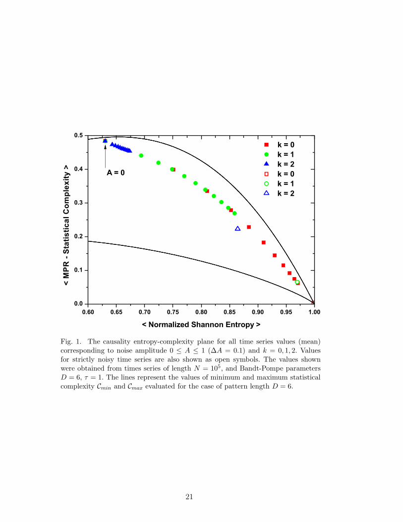
Figure 1 summarizes the planar behavior of the noisy chaotic time series con-sidered (the logistic map with additive correlated noise with f−k PS), con-sidering noise amplitudes 0 ≤ A ≤ 1 (∆A = 0.1) and k = 0 (uncorrelated),k = 1, 2 (correlated), see also Fig. 8 in [21]. Clearly, given the noise-amplitudevalues here considered, the noise has a mere perturbative role vis-a-vis of thelogistic map’s chaotic behavior.

For A = 0 we obtain the purely deterministic value corresponding to the lo-gistic time-series, localized approximately at a medium-high entropic coordi-nate, near the highest possible complexity value. Note that such is the typicalbehavior observed for deterministic systems [11]. For a purely uncorrelatedstochastic process (k = 0) we have HS = 1 and CJS = 0. The correlated (col-ored) stochastic processes (k 6= 0) yield points located at intermediate valuesbetween the curves Cmin and Cmax, with decreasing values of entropy and in-creasing values of complexity as k grows [11] (see Fig. 1, open symbols). Fromthis figure and, also from our previous work [21], we see that if k ≈ 0, forincreasing values of the amplitude A, entropy and complexity values change(starting from the value corresponding to the pure logistic series, i.e., A = 0)with a tendency to approach the values corresponding to pure noise, that is,(HS ≈ 1 and CJS ≈ 0). Similar behavior is observed when correlated noisesare considered, k 6= 0.

The main effect of the additive noise (A 6= 0) is to shift the point representativeof zero noise (A = 0) towards increasing values of entropy HS and decreasingvalues of complexity CJS. This shift defines a kind of “trajectory” (curve) inthe H × C-plane, that is located in the vicinity of the maximum complexityCmax−curve. Moreover, we found (by looking at other chaotic maps) thatthis trajectory is characteristic of the dynamical system under analysis. Suchbehavior can be linked to the persistence of forbidden patterns because they,in turn, imply that the deterministic logistic component is still operative andinfluencing the time series’ behavior [21]. As k increases, the dependence onthe noise-amplitude A (0 ≤ A ≤ 1) tends to become attenuated, implyingthat M(N,D) 6= 0 (see Fig. 4 of [21]), while it almost disappears for k ≈ 2.This fact is due to the effect of the “coloring” correlations of the noise, thatgrow with increasing values of k.

4.2 Case A ≥ 1

Here we are interested in the physics associated to A’s growth, entailing aninterchange between the roles of the logistic map and of the noise because a

8

large A makes noise the dominant feature. Several effects should be considered

• noise contamination level (represented by A),• noise correlation (represented by k) and,• persistence of the forbidden patterns.

We should expect that as A grows (with fixed values forN andD), the missing-patterns numbers would diminish and eventually vanish. With strong or verystrong noise we expect zero missing patterns and eventual predominance ofstochastic features. This means M(N,D) = 0 independently of the A value.However, taking into account our previous results [21], we expect that somenew specific features will be revealed by the use of the causality entropy-complexity plane.

Consider our results for uncorrelated noise k = 0 and increasing values of noise-amplitude A depicted in Fig. 2. This graph reveals that for A ≥ 1 the pointscorresponding to increasing values of A continue to move in the plane towardsthe site representative of pure noise, with M(N,D) = 0. The perturbativecharacter of the noise is, of course, lost. This behavior is apparent in Fig.3, where the corresponding Bandt-Pompe PDF’s, for a typical noisy chaotictime-series, are displayed for increasing noise amplitudes A. The correspondingvalue of M(N,D) can also be observed in these graphs.

At the top-left corner of Fig. 3 we depict the Bandt-Pompe’s PDF for theunperturbed logistic map (A = 0). The presence of forbidden patterns (thathave probabilities pi = 0) is clearly visible. In the same plot, at the bottom-right corner, we display the pure noise k = 0 (white noise) PDF. No forbiddenpatterns exist now, and we observe the characteristic flat distribution, pi ∼=1/M for all patterns i = 1, · · · ,M (M = D! = 720). The noise-influence on thePDFs is clearly displayed in this graph (see also the plots for k = 1 and k = 2,Figures 5 and 7). One appreciates the fact that the PDF evolves from that ofthe logistic map towards that of the pure-noise as one increases the value of A.The noise-effect also destroys the forbidden character of some patterns, whoseassociated probabilities grow slowly with the control parameter A, a featurethat emphasizes the presence of a deterministic component in the noisy timeseries, even for M(N,D) = 0, if A is not too large. This effect disappears forvery strong noise. Note that for A = 5 the PDF is practically equal to that ofpure noise. The two PDFs are almost indistinguishable at A = 10, and theirplanar localizations coincide (see Fig. 2).

In Figures 4 and 6 one can appreciate details of the planar-localization ofnoisy chaotic time-series (mean values taken over ten realizations) that emergeout of the noise-contaminated logistic map. We display values for correlatednoise with k = 1 and k = 2, with increasing noise amplitude A ≥ 1. Inthese plots we also observe the planar locations of both the time-series for the

9

unperturbed logistic map (A = 0) and the pure-correlated noise (k = 1, 2). Asin the previous case of uncorrelated noise (k = 0), the planar locations movetowards the pure-noise’s site (in the present cases, k = 1 and k = 2-pure noise,respectively) for increasing values of the noise-amplitude A. New behaviorsemerge, as reflected by Figures 4 and 6. For varying noise-amplitude values weappreciate two different trajectories: 1) displacement on the associated planarlocations from left to right (starting form the unperturbed value A = 0), untilreaching a point associated with a critical value Ac: Ac

∼= 7 for k = 1 (see Fig.4) and Ac

∼= 80 for k = 2 (see Fig. 6). 2) At these critical values the trajectoryreverses its direction (now it moves from right to left, “below” the first curve).The two trajectories converge at the planar location of the pure-correlatednoise. Identical behavior was observed for all correlated noises with k-valuesin the interval 0 < k < 2, that exhibit specific critical values of Ac(k).

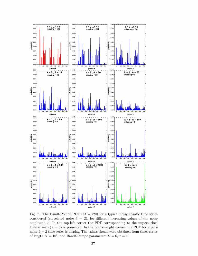
The planar behavior of the noisy, chaotic time-series can be interpreted interms of two main interacting effects, namely, those associated with a) the per-sistence and robustness of the forbidden patterns in the deterministic chaoticcomponent of the time-series and, b) the correlations characterizing stochas-tic observational noise (which in the present cases do not display forbiddenpatterns). These correlations grow with increasing values of k > 0. Lookingto the associated Bandt-Pompe’s PDFs behavior, depicted in Figs. 5 and 7for different values of A, the observed planar trajectories can be succinctlydescribed as itemized below.

• Amplitude range 0 < A ≤ Ac: We deal with a two scenarios, one (Case A)in which the correlated noise acts as a perturbation (M(N,D) 6= 0). Inthe other one (Case B) the logistic and the correlated noise have the samehierarchy (M(N,D) = 0). Fig. 6.b shows that for k = 2 and case A theentropic and complexities’ dispersion (given by the standard deviation) areboth small and due to the perturbative noise. Contrariwise, for case B thedispersion values increase with the noise amplitude A.

• Amplitude range A ≥ Ac: Now the correlated noise dominates. The deter-ministic component of the time series can be considered here as a perturba-tion. Again, for this range of noise amplitudes we have M(N,D) = 0. Wealso observe that the dispersions of the entropy Hs and the complexity CJSare small.

5 Conclusions

We have revisited in some detail the paradigmatic concept of forbidden/missingordinal patterns and used it as a tool for distinguishing between deterministicand stochastic behavior in empiric time-series. In the spirit of [13,14,15,18,19,20],we extended this kind of analysis by linking it to the physics described by the

10

causality entropy-complexity plane [11]. Our considerations were made withregards to deterministic, finite time series contaminated with additive noises ofdifferent degree of correlation. Our analysis of the noise-determinism competi-tion clearly demonstrates that forbidden patterns are a deterministic feature ofnonlinear systems and also reaffirms the usefulness of the entropy-complexityplane as a powerful tool of the theoretical arsenal.

The planar localization in the causal entropy-complexity plane describing anuncontaminated, nonlinear deterministic system is displaced, by the additionof noise, towards a zone typical of pure stochasticity. This displacement gen-erates a kind of trajectory in the H × C-plane that is located in the vicinityof the curve corresponding to maximum statistical complexity.

If the noise is uncorrelated (white noise), the displacement of the systemscharacteristic point in the H×C-plane becomes more pronounced as the noiseintensity (amplitude) increases. It exhibits a monotonic decreasing behavior(from pure determinism to pure stochasticity). The noise-effect tends to elim-inate forbidden patterns. Since these, in turn, are features of a deterministicdynamics, their destruction signals deterministic-nature’s loss.

For contaminating correlated noise a new type of planar trajectory-behavioremerges as the noise intensity increases. Starting from a pure deterministiclocalization, the trajectory converges to a pure stochastic localization by fol-lowing a loop-curve as the noise intensity increases. For a critical value ofnoise intensity (Ac), however, this trajectory reverses direction. One observesa planar-movement of the systems characteristic point that starts at the un-perturbed value (A = 0) and closely approaches the curve of maximum com-plexity, from left to right, with increasing entropic values. At the critical noiseintensity (Ac) this displacement reverses direction. It takes place now fromright to left, below the original curve and converging to the planar locationtypical of pure-correlated noise. The value of the critical intensity Ac dependson the correlation degree of the noise and on the deterministic component.

Three different scenarios can be associated:

a) The correlated noise acting as a perturbation and M(N,D) 6= 0. The netnoise effect is to destroy the forbidden character of some of the patterns.However due to the low noise intensity and to its correlations, the numberof affected patterns is relatively low. The dominance of the deterministiccomponent over the noisy one is reflected by low dispersion values forboth the entropy and the statistical complexity.

b) The deterministic and the stochastic components have the same hierar-chy andM(N,D) = 0. However, the persistent character of the forbiddenpatterns of the deterministic component and its interplay with the cor-relations present in the noise is reflected in the systems characteristic

11

point trajectory, that moves along the curve of maximum complexity, in-dicating that the pertinent patterns do not appear as frequently as theremaining ones. This behavior is indicative of a still active deterministicdynamics. The dispersion values for our two quantifiers increase with thenoise intensity.

The two scenarios above correspond to a noise intensity-range 0 ≤ A ≤ Ac.

c) The noisy component is the dominating one and the deterministic partcan be considered as a perturbation. This scenario corresponds to thenoise intensity range A ≥ Ac and we have M(N,D) = 0 as well, withlow dispersion values for entropy and statistical complexity.

6 Appendix

6.1 MPR-Statistical Complexity

Given any arbitrary discrete probability distribution P = pi : i = 1, · · · ,M,with M the number of freedom-degrees, Shannon’s logarithmic informationmeasure reads [28]

S[P ] = −M∑

i=1

pi ln(pi) . (3)

The Shannon entropy is a measure of the uncertainty associated to the phys-ical process described by P . It is widely known that an entropic measuredoes not quantify the degree of structure or patterns present in a process [29].Other measures of statistical or structural complexity, able capture their orga-nizational properties, are necessary for a better understanding of chaotic timeseries [30]. Our group introduced an effective statistical complexity measure(SCM) that is able to detect essential details of the dynamics and differentiatedifferent degrees of periodicity and chaos [31]. This specific SCM, abbrevi-ated as the MPR-complexity one, provides important additional informationregarding the peculiarities of the underlying probability distribution, not al-ready detected by the entropy. It is defined, following the seminal, intuitivenotion advanced by Lopez-Ruiz et al. [32], via

CJS[P ] = QJ [P, Pe] · HS[P ], (4)

using:

12

a) The normalized Shannon entropy (0 ≤ HS ≤ 1)

HS[P ] = S[P ]/Smax , (5)

where Smax = S[Pe] = lnM and Pe = 1/M, · · · , 1/M the uniform distri-bution.

b) The so-called disequilibrium QJ (0 ≤ QJ ≤ 1), a quantifier defined in termsof the extensive (in the thermodynamical sense) Jensen-Shannon divergenceJ [P, Pe] that links two PDFs. We have

QJ [P, Pe] = Q0 · J [P, Pe] , (6)

with

J [P, Pe] = S [(P + Pe)/2]− S[P ]/2− S[Pe]/2 . (7)

Q0 is a normalization constant, equal to the inverse of the maximum possiblevalue of J [P, Pe]. This value is obtained when one of the values of P , saypm, is equal to one and the remaining pi values are equal to zero, i.e.,

Q0 = − 2(

M + 1

M

)

ln(M + 1)− 2 ln(2M) + lnM

−1

. (8)

The Jensen-Shannon divergence, that quantifies the difference between two(or more) probability distributions, is especially useful to compare the symbol-composition of different sequences [33]. The complexity measure constructedin this way has the intensive property found in many thermodynamic quan-tities [31]. We stress the fact that the statistical complexity defined above isthe product of two normalized entropies (the Shannon entropy and Jensen-Shannon divergence), but it is a nontrivial function of the entropy because itdepends on two different probabilities distributions, i.e., the one correspondingto the state of the system, P , and the uniform distribution, Pe.

6.2 Entropy-Complexity plane

The time-evolution of the MPR-complexity can be analyzed using a diagramof CJS versus time t. Thermodynamics’ second law states that for isolatedsystems the entropy grows monotonically with time (dHS/dt ≥ 0), entailingthat HS can be viewed an “arrow of time” [34]. This suggests to study thetemporal evolution of the SCM via an analysis of CJS versus HS. A normalizedentropy-axis substitutes for the time-axis. Since one knows that for a givenvalue of HS the range of possible MPR-complexity values varies between aminimum Cmin and a maximum Cmax [35], our evolutionary path must takeplace in the planar-region delimited by these curves. It was demonstrated

13

that evolutionary path analysis generates insight into the details of the sys-tems probability distribution (not provided by randomness measures like theentropy [11,30]) that helps to uncover information related to the correlationalstructure between the components of a given physical process [36,37].

6.3 Estimation of the Probability Distribution Function

Before attempting the time series characterization using Information Theoryquantifiers, a probability distribution function (PDF) associated to the timeseries under analysis should be provided beforehand. The determination ofthe most adequate PDF is a fundamental problem because P and the samplespace Ω are inextricably linked. Many methods have been proposed for aproper selection of the probability space (Ω, P ). We can mention: (a) frequencycounting [38], (b) procedures based on amplitude statistics [39], (c) binarysymbolic dynamics [40], (d) Fourier analysis [41] and, (e) wavelet transform[42], among others. Their applicability depends on particular characteristics ofthe data, such as stationarity, time series length, variation of the parameters,level of noise contamination, etc. In all these cases the dynamics’ global aspectscan be somehow captured, but the different approaches are not equivalentin their ability to discern all the relevant physical details. One must alsoacknowledge the fact that the above techniques are introduced in a rather “adhoc fashion” and they are not directly derived from the dynamical propertiesthemselves of the system under study.

A better procedure is provided by the symbolic analysis of the time series,that discretizes the raw series and transforms it into a sequence of symbols.Symbolic analysis is efficient for nonlinear data processing, with low sensitivityto noise [43]. Of course, meaningful symbolic representations of the originalseries are not provided by God and require some effort [44,45]. Today manypeople are confident that the Bandt and Pompe approach for generating PDF’sis one of the most simple symbolization techniques and takes into accounttime-causality in the evaluation of the PDF associated to a time series [12].Symbolic data are i) created by associating a rank to the series-values andii) defined by reordering the embedded data in ascending order. Data arereconstructed with an embedding dimension D. In this way it is possible toquantify the diversity of the ordering symbols (patterns) derived from a timeseries, evaluating the so called “permutation entropy” HS, and permutationstatistical complexity CJS (i.e., the normalized Shannon entropy and MPR-statistical complexity measure evaluated for the Bandt and Pompe’s PDF).

14

6.4 The Bandt and Pompe approach for PDF construction

Bandt and Pompe [12] introduced a simple and robust method to evaluatethe probability distribution taking into account the time causality of the sys-tem dynamics. They suggested that the symbol sequence should arise natu-rally from the time series, without any model-based assumptions. Thus, theytook partitions by comparing the order of neighboring values rather thanpartitioning the amplitude into different levels. That is, given a time seriesS = xt; t = 1, · · · , N, an embedding dimension D > 1 (D ∈ N), and anembedding time delay τ (τ ∈ N), the ordinal pattern of order D generated by

s 7→(

xs−(D−1)τ , xs−(D−2)τ , · · · , xs−τ , xs

)

, (9)

is to be considered. To each time s we assign a D-dimensional vector that re-sults from the evaluation of the time series at times s− (D− 1)τ, · · · , s− τ, s.Clearly, the higher the value of D, the more information about the past isincorporated into the ensuing vectors. By the ordinal pattern of order Drelated to the time s we mean the permutation π = (r0, r1, · · · , rD−1) of(0, 1, · · · , D − 1) defined by

xs−rD−1τ ≤ xs−rD−2τ ≤ · · · ≤ xs−r1τ ≤ xs−r0τ . (10)

In this way the vector defined by Eq. (9) is converted into a unique symbol π.In order to get a unique result we consider that ri < ri−1 if xs−riτ = xs−ri−1τ .This is justified if the values of xt have a continuous distribution so that equalvalues are very unusual.

For all the D! possible orderings (permutations) πi when the embedding di-mension is D, their associated relative frequencies can be naturally computedby the number of times this particular order sequence is found in the timeseries divided by the total number of sequences,

p(πi) =♯s|s ≤ N − (D − 1)τ ; (s) has type πi

N − (D − 1)τ. (11)

In the last expression the symbol ♯ stands for “number”. Thus, an ordinalpattern probability distribution P = p(πi), i = 1, · · · , D! is obtained fromthe time series.

It is clear that this ordinal time-series’ analysis entails losing some details ofthe original amplitude-information. Nevertheless, a meaningful reduction ofthe complex systems to their basic intrinsic structure is provided. Symboliz-ing time series, on the basis of a comparison of consecutive points allows for

15

an accurate empirical reconstruction of the underlying phase-space of chaotictime-series affected by weak (observational and dynamical) noise [12]. Further-more, the ordinal-pattern probability distribution is invariant with respect tononlinear monotonous transformations. Thus, nonlinear drifts or scalings ar-tificially introduced by a measurement device do not modify the quantifiers’estimations, a relevant property for the analysis of experimental data. Theseadvantages make the BP approach more convenient than conventional meth-ods based on range partitioning. Additional advantages of the Bandt andPompe method reside in its simplicity (we need few parameters: the patternlength/embedding dimension D and the embedding time lag τ) and the ex-tremely fast nature of the pertinent calculation-process [46,47]. We stress thatthe Bandt and Pompe’s methodology is not restricted to time series repre-sentative of low dimensional dynamical systems but can be applied to anytype of time series (regular, chaotic, noisy, or reality based), with a very weakstationary assumption (for k = D, the probability for xt < xt+k should notdepend on t [12]).

The probability distribution P is obtained once we fix the embedding di-mension D and the embedding time delay τ . The former parameter plays animportant role for the evaluation of the appropriate probability distribution,since D determines the number of accessible states, given by D!. Moreover, ithas been established that the length N of the time series must satisfy the con-dition N ≫ D! in order to achieve a proper differentiation between stochasticand deterministic dynamics [11]. With respect to the selection of the param-eters, Bandt and Pompe suggest in their cornerstone paper [12] to work with3 ≤ D ≤ 7 with a time lag τ = 1. Nevertheless, other values of τ might provideadditional information. Soriano et al. [48,49] and Zunino et al. [50] recentlyshowed that this parameter is strongly related, when it is relevant, with theintrinsic time scales of the system under analysis. In the present work D = 6and τ = 1 are used. Of course it is also assumed that enough data are availablefor a correct embedding-time delay procedure (attractor-reconstruction).

Acknowledgments

This research has been partially supported by a scholarship from The Univer-sity of Newcastle awarded to Laura C. Carpi. Patricia M. Saco acknowledgessupport from the Australian Research Council, ARC, Australia. Osvaldo A.Rosso gratefully acknowledges support from CAPES, PVE fellowship, Brazil.Martın Gomez Ravetti acknowledges support from FAPEMIG and CNPq,Brazil.

16

References

[1] A. R. Osborne, A. Provenzale, Finite correlation dimension for stochastic systemswith power-law spectra. Physica D 35 (1989) 357–381.

[2] G. Sugihara, R. M. May, Nonlinear forecasting as a way of distinguishing chaosfrom measurement error in time series. Nature 344 (1983) 734–741.

[3] D. T. Kaplan, L. Glass, Direct test for determinism in a time series. Phys. Rev.Lett. 68 (1992) 427–430.

[4] D. T. Kaplan, L. Glass, Coarse-grained embeddings of time series: random walks,Gaussian random processes, and deterministic chaos. Physica D 64 (1993) 431–454.

[5] H. Kantz, E. Olbrich, Coarse grained dynamical entropies: Investigation of high-entropic dynamical systems. Physica A 280 (2000) 34–48.

[6] M. Cencini, M. Falcioni, E. Olbrich, H. Kantz, A. Vulpiani, Chaos or noise:Difficulties of a distinction. Physica A 280 (2000) 34–48.

[7] H. Kantz, T. Scheiber, Nonlinear Time Series Analysis. Cambridge UniversityPress, Cambridge, UK, 2002.

[8] H. D. I. Abarbanel, Analysis of Observed Chaotic Data. Springer-Verlag, NewYork, USA, 1996.

[9] A. N. Kolmogorov, A new metric invariant for transitive dynamical systems andautomorphisms in lebesgue sapces. Dokl. Akad. Nauk., USSR , 119 (1959) 861 –864.

[10] Y. G. Sinai, On the concept of entropy for a dynamical system. Dokl. Akad.Nauk., USSR , 124 (1959) 768 – 771.

[11] O. A. Rosso, H. A Larrondo, M. T. Martın, A. Plastino, M. A. Fuentes,Distinguishing noise from chaos. Phys. Rev. Lett. 99 (2007) 154102.

[12] C. Bandt, B. Pompe, Permutation entropy: a natural complexity measure fortime series. Phys. Rev. Lett. 88 (2002) 174102.

[13] J. M. Amigo, L. Kocarev, J. Szczepanski, Order patterns and chaos Phys. Lett.A 355 (2006) 27-31.

[14] J. M. Amigo, S. Zambrano, M. A. F. Sanjuan, True and false forbidden patternsin deterministic and random dynamics. Europhys. Lett. 79 (2007) 50001.

[15] J. M. Amigo, S. Zambrano and M. A. F. Sanjuan, Combinatorial detection ofdeterminism in noisy time series. Europhys. Lett. 83 (2008) 60005.

[16] J. M. Amigo, Permutation complexity in dynamical systems. Springer-Verlag,Berlin, Germany, 2010.

17

[17] L. C. Carpi, P. M. Saco, O. A. Rosso, Missing Ordinal Patterns in CorrelatedNoises. Physica A 389 (2010) 2020–2029.

[18] M. Zanin, Forbidden patterns in financial time series. Chaos 18 (2008) 013119.

[19] L. Zunino, M. Zanin, B. M. Tabak, D. Perez, O. A. Rosso, Forbidden patterns,permutation entropy and stock market inefficiency. Physica A 388 (2009) 2854 –2864.

[20] G. Ouyang, X. Li, C. Dang and D. A. Richards, Deterministic dynamics ofneural activity during absence seizures in rats. Phys. Rev. E 79 (2009) 041146.

[21] O.A. Rosso, L. C. Carpi, M. P. Saco, M. Gomez Ravetti, A. Plastino, H. A.Larrondo. Causality and the entropy-complexity plane: robustness and missingordinal patters. Physica A (2011) in press, DOI: 10.1016/j.physa.2011.07.030

[22] O. A. Rosso, L. De Micco, H. Larrondo, M. T. Martın, A. Plastino. Generalizedstatistical complexity measure. Int. J. Bif. and Chaos 20 (2010) 775–785.

[23] J. C. Sprott, Chaos and Time Series Analysis, Oxford University Press, Oxford,2004.

[24] M. Matsumoto, T. Nishimura, Mersenne twister: a 623-dimensionally uniformpseudo-random number generator. ACM Transactions on Modeling and ComputerSimulation 8 (1998) 3 – 30.

[25] H. Wold, A Study in the Analysis of Stationary Time Series. Almqvist andWiksell, Upsala, Sweden, 1938.

[26] J. Kurths, H. Herzel, An attractor in a solar time series. Physica D 25 (1987)165 – 172.

[27] S. Cambanis, C. D. Hardin, A. Weron, Innovations and Wold decompositionsof stable sequences. Probab. Theory Relat. Fields 79 (1988) 1 – 27.

[28] C. Shannon, W. Weaver, The Mathematical Theory of CommunicationUniversity of Illinois Press, Champaign, IL, 1949.

[29] D. P. Feldman, J. P. Crutchfield, Measures of statistical complexity: Why?.Phys. Lett. A 238 (1998) 244 – 252.

[30] D. P. Feldman, C. S. McTague, J. P. Crutchfield, The organization ofintrinsic computation: Complexity-entropy diagrams and the diversity of naturalinformation processing. Chaos 18 (2008) 043106.

[31] P. W. Lamberti, M. T. Martın, A. Plastino, and O. A. Rosso, Intensive entropicnontriviality measure. Physica A 334 (2004) 119 – 131.

[32] R. Lopez-Ruiz, H. L. Mancini, X. Calbet, A statistical measure of complexity.Phys. Lett. A 209 (1995) 321 – 326.

[33] I. Grosse, P. Bernaola-Galvan, P. Carpena, R. Roman-Roldan, J. Oliver, H.E. Stanley, Analysis of symbolic sequences using the Jensen-Shannon divergence.Phys. Rev. E 65 (2002) 041905.

18

[34] A. R. Plastino, and A. Plastino, Symmetries of the Forker-Plank equation andFisher-Frieden arrow of time. Phys. Rev. E 54 (1996) 4423 – 4326.

[35] M. T. Martın, A. Plastino, O. A. Rosso, Generalized statistical complexitymeasures: geometrical and analytical properties. Physica A 369, 439 (2006) 439 –462.

[36] O. A. Rosso, C. Masoller. Detecting and quantifying stochastic and coherenceresonances via Information Theory complexity measurements. Phys. Rev. E 79(2009) 040106(R).

[37] O. A. Rosso, C. Masoller. Detecting and quantifying temporal correlations instochastic resonance via Information Theory measures. European Phys. JournalB, 69 (2009) 37–43.

[38] O. A. Rosso, H. Craig, P. Moscato, Shakespeare and other English renaissanceauthors as characterized by Information Theory complexity quantifiers. PhysicaA 388 (2009) 916 – 926

[39] L. De Micco, C. M. Gonzalez, H. A. Larrondo, M. T. Martın, A. Plastino, O. A.Rosso, Randomizing nonlinear maps via symbolic dynamics. Physica A 87 (2008)3373 - 3383.

[40] K. Mischaikow, M. Mrozek, J. Reiss, A. Szymczak, Construction of symbolicdynamics from experimental time series. Phys. Rev. Lett. 82 (1999) 1114 - 1147.

[41] G. E. Powell, I. C. Percival, A spectral entropy method for distinguishing regularand irregular motion of hamiltonian systems. J. Phys. A: Math. Gen. 12 (1979)2053 - 2071.

[42] O. A. Rosso, S. Blanco, J. Jordanova, V. Kolev, A. Figliola, M. Schurmann, E.Basar, Wavelet entropy: a new tool for analysis of short duration brain electricalsignals. J. Neurosc. Meth. 105 (2001) 65-75.

[43] J. M. Finn, J. D. Goettee, Z. Toroczkai, M. Anghel, B. P. Wood, Estimationof entropies and dimensions by nonlinear symbolic time series analysis. Chaos 13,444 (2003) 444 – 457.

[44] E. M. Bollt, T. Stanford, Y. C. Lai, K. Zyczkowski, Validity of Threshold-Crossing Analysis of Symbolic Dynamics from Chaotic Time Series. Phys. Rev.Lett. 85 (2000) 3524 – 3527.

[45] C. S. Daw, C. E. A. Finney, E. R. Tracy, A review of symbolic analysis ofexperimental data. Rev. Sci. Instrum. 74 (2003) 915 – 931.

[46] K. Keller, M. Sinn. Ordinal analysis of time series. Physica A 356 (2005) 114–120.

[47] K. Keller, H. Lauffer. Symbolic analysis of high-dimensional time series. Int. J.Bifurcation and Chaos 13 (2003) 2657–2668.

[48] M. C. Soriano, L. Zunino, L. Larger, I. Fischer, and C. R. Mirasso ). opto-electronic oscillator. Optics Letters 36 (2010) 2212–2214.

19

[49] M. C. Soriano, M. C., L. Zunino, O. A. Rosso, I. Fischer, C. R. Mirasso. Timescales of a chaotic semiconductor laser with optical feedback under the lens of apermutation information analysis. IEEE J. Quantum Electron. 47 (2010) 252–261.

[50] L. Zunino, M. C. Soriano, I. Fischer, O. A. Rosso, C. R. Mirasso. Permutationinformation theory approach to unveil delay dynamics from time series analysis.Phys. Rev. E 82 (2010) 046212.

20

0.60 0.65 0.70 0.75 0.80 0.85 0.90 0.95 1.000.0

0.1

0.2

0.3

0.4

0.5 k = 0 k = 1 k = 2 k = 0 k = 1 k = 2

< M

PR -

Stat

istic

al C

ompl

exity

>

< Normalized Shannon Entropy >

A = 0

Fig. 1. The causality entropy-complexity plane for all time series values (mean)corresponding to noise amplitude 0 ≤ A ≤ 1 (∆A = 0.1) and k = 0, 1, 2. Valuesfor strictly noisy time series are also shown as open symbols. The values shownwere obtained from times series of length N = 105, and Bandt-Pompe parametersD = 6, τ = 1. The lines represent the values of minimum and maximum statisticalcomplexity Cmin and Cmax evaluated for the case of pattern length D = 6.

21

0.60 0.65 0.70 0.75 0.80 0.85 0.90 0.95 1.000.0

0.1

0.2

0.3

0.4

0.5

< M

PR -

Stat

istic

al C

ompl

exity

>

< Normalized Shannon Entropy >

( a )

k = 0A = 0

A = 1

pure noise

0.995 0.996 0.997 0.998 0.9990.000

0.002

0.004

0.006

0.008

0.010

pure noise

A = 5

A = 10

k = 0

( b )

< M

PR -

Stat

istic

al C

ompl

exity

>

< Normalized Shannon Entropy >

Fig. 2. a ) The causality entropy-complexity plane for all time series values (mean)corresponding to increasing values of noise amplitude A and k = 0. Value for the caseof strictly noisy time series is shown as open symbol. The values shown were obtainedfrom times series of length N = 105, and Bandt-Pompe parameters D = 6, τ = 1.The lines represent the values of minimum and maximum statistical complexityCmin and Cmax evaluated for the case of pattern length D = 6. b) Detail for highentropy values.

22

0 100 200 300 400 500 600 7000.000

0.005

0.010

0.015

0.020

0.025

0.030

0.035

0.040

0.045

pro

babi

lity

pattern #

missing = 645 k = 0 , A = 0

0 100 200 300 400 500 600 7000.000

0.005

0.010

0.015

0.020

0.025

0.030

0.035

0.040

0.045

missing = 85

k = 0 , A = 0.1

prob

abili

ty

pattern #

0 100 200 300 400 500 600 7000.000

0.005

0.010

0.015

0.020

0.025

0.030

0.035

0.040

0.045

missing = 10k = 0 , A = 0.3

prob

abili

ty

pattern #

0 100 200 300 400 500 600 7000.000

0.005

0.010

0.015

0.020

0.025

0.030

0.035

0.040

0.045

missing = 0k = 0 , A = 0.5

prob

abili

ty

pattern #

0 100 200 300 400 500 600 7000.000

0.005

0.010

0.015

0.020

0.025

0.030

0.035

0.040

0.045

missing = 0k = 0 , A = 0.7

prob

ability

pattern #

0 100 200 300 400 500 600 7000.000

0.005

0.010

0.015

0.020

0.025

0.030

0.035

0.040

0.045

prob

ability

pattern #

missing = 0 k = 0 , A = 1

0 100 200 300 400 500 600 7000.000

0.005

0.010

0.015

0.020

0.025

0.030

0.035

0.040

0.045

prob

ability

pattern #

missing = 0 k = 0 , A = 5

0 100 200 300 400 500 600 7000.000

0.005

0.010

0.015

0.020

0.025

0.030

0.035

0.040

0.045

prob

ability

pattern #

missing = 0

k= 0 - pure

Fig. 3. The Bandt-Pompe PDF (M = 720) for a typical noisy chaotic time seriesconsidered (uncorrelated noise k = 0), for different increasing values of the noiseamplitude A. In the top-left corner the PDF corresponding to the unperturbedlogistic map (A = 0) is presented. In the bottom-right corner, the PDF for a purenoise k = 0 time series is display. The values shown were obtained from times seriesof length N = 105, and Bandt-Pompe parameters D = 6, τ = 1.

23

0.60 0.65 0.70 0.75 0.80 0.85 0.90 0.95 1.000.0

0.1

0.2

0.3

0.4

0.5

pure noise

A = 7

A = 1

< M

PR -

Stat

istic

al C

ompl

exity

>

< Normalized Shannon Entropy >

k = 1.0

( a )

A = 0

0.968 0.970 0.972 0.974 0.976 0.978 0.980 0.9820.040

0.045

0.050

0.055

0.060

0.065

0.070

( b )

A = 5

A = 7A = 10

A = 30

A = 50

A = 100A = 300

pure noise k = 1.0

< M

PR -

Stat

istic

al C

ompl

exity

>

< Normalized Shannon Entropy >

Fig. 4. a) The causality entropy-complexity plane for all time series values (mean)corresponding to increasing values of noise amplitude A and k = 1. Value for the caseof strictly noisy time series is shown as open symbol. The values shown were obtainedfrom times series of length N = 105, and Bandt-Pompe parameters D = 6, τ = 1.The lines represent the values of minimum and maximum statistical complexityCmin and Cmax evaluated for the case of pattern length D = 6. b) Detail for highentropy values.

24

0 100 200 300 400 500 600 7000.000

0.005

0.010

0.015

0.020

0.025

0.030

0.035

0.040

0.045

prob

ability

pattern #

missing = 645 k = 1 , A = 0

0 100 200 300 400 500 600 7000.000

0.005

0.010

0.015

0.020

0.025

0.030

0.035

0.040

0.045

prob

ability

pattern #

missing = 3 k = 1 , A = 1

0 100 200 300 400 500 600 7000.000

0.005

0.010

0.015

0.020

0.025

0.030

0.035

0.040

0.045

prob

ability

pattern #

missing = 0 k = 1 , A = 5

0 100 200 300 400 500 600 7000.000

0.005

0.010

0.015

0.020

0.025

0.030

0.035

0.040

0.045

prob

ability

pattern #

missing = 0 k = 1 , A = 7

0 100 200 300 400 500 600 7000.000

0.005

0.010

0.015

0.020

0.025

0.030

0.035

0.040

0.045

prob

ability

pattern #

missing = 0 k = 1 , A = 10

0 100 200 300 400 500 600 7000.000

0.005

0.010

0.015

0.020

0.025

0.030

0.035

0.040

0.045

prob

ability

pattern #

missing = 0 k = 1 , A = 50

0 100 200 300 400 500 600 7000.000

0.005

0.010

0.015

0.020

0.025

0.030

0.035

0.040

0.045

prob

ability

pattern #

missing = 0 k = 1 , A = 100

0 100 200 300 400 500 600 7000.000

0.005

0.010

0.015

0.020

0.025

0.030

0.035

0.040

0.045

prob

ability

pattern #

missing = 0 k = 1 - pure

Fig. 5. The Bandt-Pompe PDF (M = 720) for a typical noisy chaotic time seriesconsidered (correlated noise k = 1), for different increasing increasing values of thenoise amplitude A. In the top-left corner the PDF corresponding to the unperturbedlogistic map (A = 0) is presented. In the bottom-right corner, the PDF for a purenoise k = 1 time series is display. The values shown were obtained from times seriesof length N = 105, and Bandt-Pompe parameters D = 6, τ = 1.

25

0.60 0.65 0.70 0.75 0.80 0.85 0.90 0.95 1.000.0

0.1

0.2

0.3

0.4

0.5

A=200A=300

A=400A=500

A=5000

A=100

A=80A=50

A=40A=30A=20

A=2 A=10

A=5A=1A=0.5

k = 2<

MPR

- St

atis

tical

Com

plex

ity >

< Normalized Shannon Entropy >

A=0

pure noise

(a)

0.60 0.65 0.70 0.75 0.80 0.85 0.90 0.95 1.000.0

0.1

0.2

0.3

0.4

0.5

(b)

A=5000

pure noise

A=0k = 2

MPR

- St

atis

tical

Com

plex

ity

Normalized Shannon Entropy

Fig. 6. a) The causality entropy-complexity plane for all time series values (mean)corresponding to increasing values of noise amplitude A and k = 2. Value for the caseof strictly noisy time series is shown as open symbol. The values shown were obtainedfrom times series of length N = 105, and Bandt-Pompe parameters D = 6, τ = 1.The lines represent the values of minimum and maximum statistical complexityCmin and Cmax evaluated for the case of pattern length D = 6. b) Same, showingmean values and standard deviation for each A considered value.

26

0 100 200 300 400 500 600 7000.000

0.005

0.010

0.015

0.020

0.025

0.030

0.035

0.040

0.045

missing = 645 pr

obab

ility

pattern #

k = 2 , A = 0

0 100 200 300 400 500 600 7000.000

0.005

0.010

0.015

0.020

0.025

0.030

0.035

0.040

0.045

missing = 296 k = 2 , A = 1

prob

ability

pattern #

0 100 200 300 400 500 600 7000.000

0.005

0.010

0.015

0.020

0.025

0.030

0.035

0.040

0.045

missing = 174 k = 2 , A = 5

prob

ability

pattern #

0 100 200 300 400 500 600 7000.000

0.005

0.010

0.015

0.020

0.025

0.030

0.035

0.040

0.045

missing = 93 k = 2 , A = 10

prob

ability

pattern #

0 100 200 300 400 500 600 7000.000

0.005

0.010

0.015

0.020

0.025

0.030

0.035

0.040

0.045

missing = 29 k = 2 , A = 20

prob

ability

pattern #

0 100 200 300 400 500 600 7000.000

0.005

0.010

0.015

0.020

0.025

0.030

0.035

0.040

0.045

missing = 0 k = 2 , A = 50

prob

ability

pattern #

0 100 200 300 400 500 600 7000.000

0.005

0.010

0.015

0.020

0.025

0.030

0.035

0.040

0.045

missing = 0 k = 2 , A = 80

prob

ability

pattern #

0 100 200 300 400 500 600 7000.000

0.005

0.010

0.015

0.020

0.025

0.030

0.035

0.040

0.045

missing = 0 k = 2 , A = 100

prob

ability

pattern #

0 100 200 300 400 500 600 7000.000

0.005

0.010

0.015

0.020

0.025

0.030

0.035

0.040

0.045

missing = 0 k = 2 , A = 300

prob

ability

pattern #

0 100 200 300 400 500 600 7000.000

0.005

0.010

0.015

0.020

0.025

0.030

0.035

0.040

0.045

missing = 0 k = 2 , A = 500

prob

ability

pattern #

0 100 200 300 400 500 600 7000.000

0.005

0.010

0.015

0.020

0.025

0.030

0.035

0.040

0.045

missing = 0 k = 2 , A = 5000

prob

ability

pattern #

0 100 200 300 400 500 600 7000.000

0.005

0.010

0.015

0.020

0.025

0.030

0.035

0.040

0.045

missing = 0 k= 2 - pure

prob

ability

pattern #

Fig. 7. The Bandt-Pompe PDF (M = 720) for a typical noisy chaotic time seriesconsidered (correlated noise k = 2), for different increasing values of the noiseamplitude A. In the top-left corner the PDF corresponding to the unperturbedlogistic map (A = 0) is presented. In the bottom-right corner, the PDF for a purenoise k = 2 time series is display. The values shown were obtained from times seriesof length N = 105, and Bandt-Pompe parameters D = 6, τ = 1.

27