
NMR Studies of Phase Behaviour - in Polyacrylonitrile Solutions
161
NMR Studies of Phase Behaviour in Polyacrylonitrile Solutions by John Anthony Golightly, B. Sc. Thesis submitted to the University of Nottingham for the degree of Doctor of Philosophy, October 1998
-
Upload
khangminh22 -
Category
Documents
-
view
0 -
download
0
Transcript of NMR Studies of Phase Behaviour - in Polyacrylonitrile Solutions
NMR Studies of Phase Behaviour
in Polyacrylonitrile Solutions
by
John Anthony Golightly, B. Sc.
Thesis submitted to the University of Nottingham for the degree of Doctor of Philosophy, October 1998

Declaration
I declare that the work contained in this thesis submitted by me, for the degree of Doctor of Philosophy, is my own original work, except where due reference is made to other authors, and has not previously been submitted by me for a degree at this, or any other university.
e'
ýý, r . i J. A. Golightly
Contents
1 Introduction 1 1.1 Aims of the thesis 1 1.2 Background 2 1.3 Fibre Spinning processes 2 1.4 Polyacrylonitrile 7
1.4.1 Structure 7 1.4.2 Solvents and the solution state of PAN 9 1.4.3 Spinning acrylic fibres 10
2 NMR Theory 13 2.1 Introduction 13 2.2 Background 13 2.3 Magnetic Moments 14 2.4 Nuclear Energy Levels 15 2.5 Resonance 16
2.5.1 Larmor Precession 17 2.5.2 Radio-frequency Excitation 19 2.5.3 Rotating Frame of Reference 19
2.6 Pulse and Fourier NMR 21 2.6.1 The Fourier Transform 21 2.6.2 Pulse experiments 22
2.7 Relaxation and the Bloch Equations 23 2.8 The Spectrometer 25
2.8.1 The NMR Probe 25 2.8.2 The r. f. Transmitter 27 2.8.3 The r. f. Receiver 28
3 NMR Relaxation Studies of PAN solutions 29 3.1 Introduction 29 3.2 Mechanisms 29
3.2.1 General Principles 29 3.2.2 B. P. P. Theory 32
3.3 Pulsed NMR Techniques 34 3.3.1 Longitudinal Relaxation 34 3.3.2 Transverse Relaxation 35
3.4 Experimental Methodology 38 3.4.1 Sample Preparation 38 3.4.2 Instrumentation 40 3.4.3 Data Fitting Programs 41
3.5 Longitudinal Relaxation in PAN solutions 47
3.5.1 Concentration Studies 47 3.5.2 Temperature Studies 49
3.6 Transverse Relaxation in PAN solutions 51 3.6.1 Concentration Studies 51 3.6.2 Temperature Studies 52
4 Self Diffusion Measurements 54 4.1 Introduction 54 4.2 Self Diffusion 55
4.2.1 General 55 4.2.2 Diffusion in Polymer Solutions 57
4.3 NMR Pulsed Field Gradient Theory 60 4.3.1 Pulsed Field Gradient Spin Echo Experiment 60 4.3.2 Pulsed Field Gradient Stimulated Echo Experiment 63
4.4 Experimental 65 4.4.1 Gradient calibration 65 4.4.2 PFGSTE Parameters 66
4.5 Results 67 4.5.1 Data Fitting 67 4.5.2 Solvent Diffusion 69 4.5.3 Applying the Diffusion Models 70 4.5.4 Polymer Diffusion 75
5 NMR Study of PAN Coagulation 77 5.1 Introduction to polymer coagulation 77 5.2 Theoretical 79
5.2.1 Phase separation 79 5.2.2 Kinetics of diffusion 86
5.3 Experimental 87 5.3.1 The concept of NMR imaging 87 5.3.2 One-dimensional gradient spin-echo experiment 88 5.3.3 NMR imaging on the MARAN-20 89
5.4 Results 94 5.5 Modelling data 98
5.5.1 Model A 98 5.5.2 Model B 100 5.5.3 Fitting data to the models 103 5.5.4 Validity of models 105 5.5.5 Discussion of Results 106
6 The Porous Nature of Wet-Spun Acrylic Fibres 111 6.1 Background ill 6.2 Film Preparation 113 6.3 NMR Transverse Relaxation Studies 114
6.3.1 The Method 114 6.3.2 Results 114
6.4 NMR Diffusion Studies 119 6.4.1 Background 119 6.4.2 Experimental Results 121
6.5 SEM of Cast PAN Films 123 6.5.1 SEM Sample Preparation 123 6.5.2 Experimental 125 6.5.3 Micrographs 125
7 Conclusions 132 7.1 NMR Relaxation Studies of PAN solutions 132 7.2 Self Diffusion Studies 134 7.3 NMR Study of PAN Coagulation 136 7.4 The Porous Nature of Wet-Spun Acrylic Fibres 138
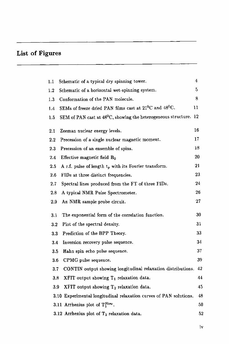
List of Figures
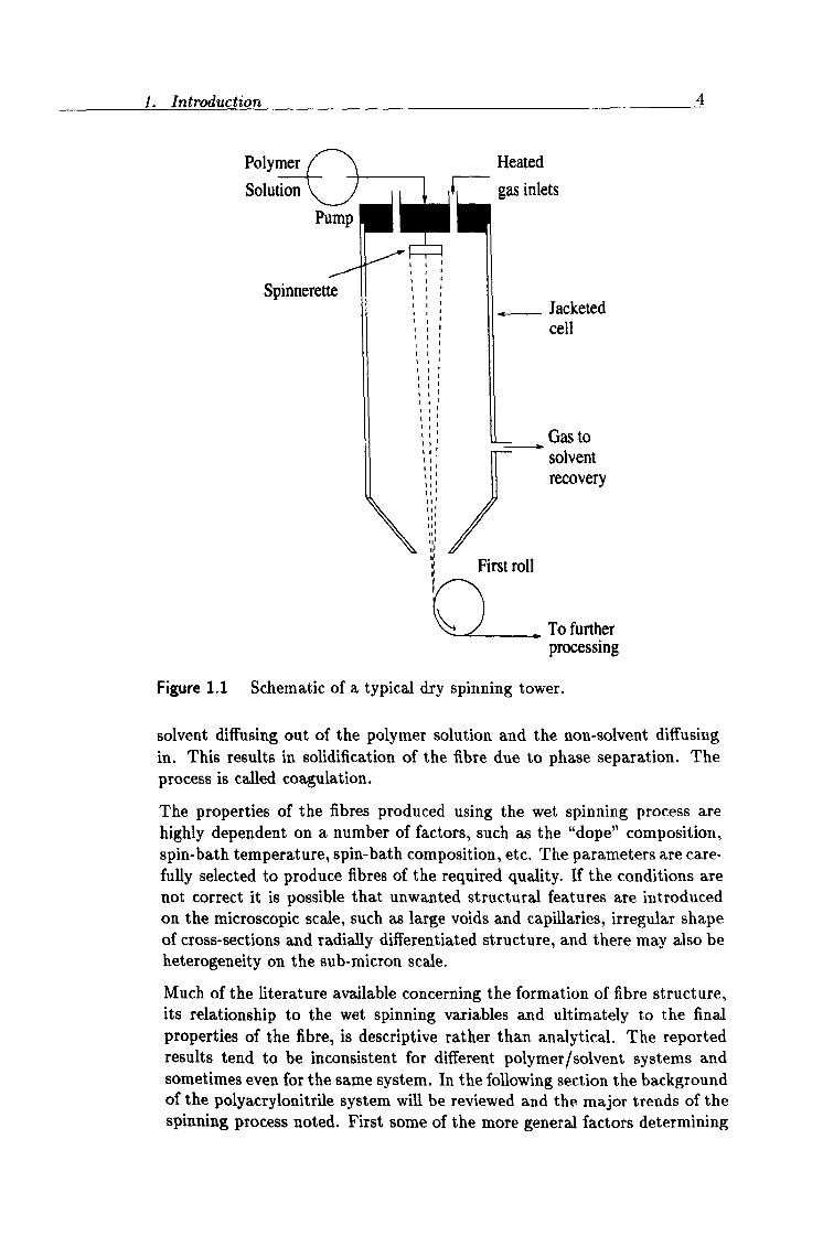
1.1 Schematic of a typical dry spinning tower. 4
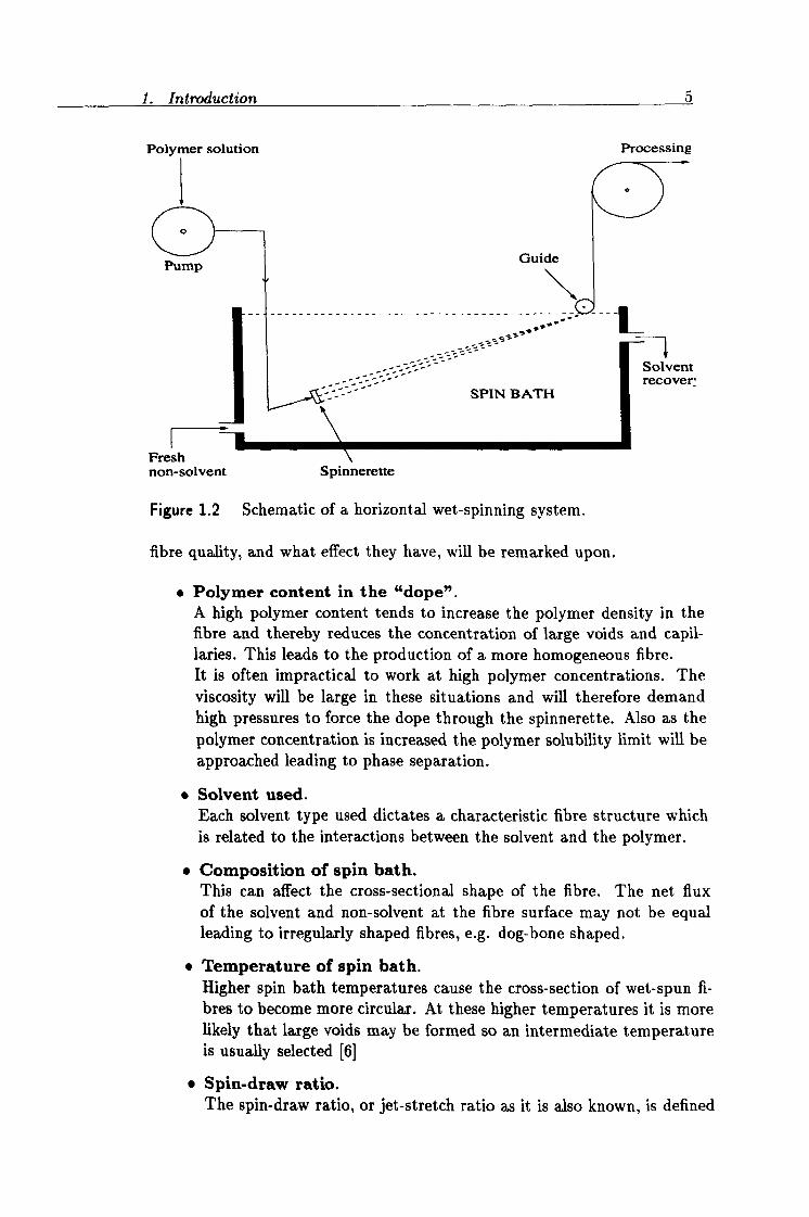
1.2 Schematic of a horizontal wet-spinning system. 5
1.3 Conformation of the PAN molecule. 8
1.4 SEMs of freeze dried PAN films cast at 21°C and 48°C. 11
1.5 SEM of PAN cast at 48°C, showing the heterogeneous structure. 12
2.1 Zeeman nuclear energy levels. 16
2.2 Precession of a single nuclear magnetic moment. 17
2.3 Precession of an ensemble of spins. 18
2.4 Effective magnetic field Bo 20
2.5 A r. f. pulse of length tp with its Fourier transform. 21
2.6 FIDs at three distinct frequencies. 23
2.7 Spectral lines produced from the FT of three FIDs. 24
2.8 A typical NMR Pulse Spectrometer. 26
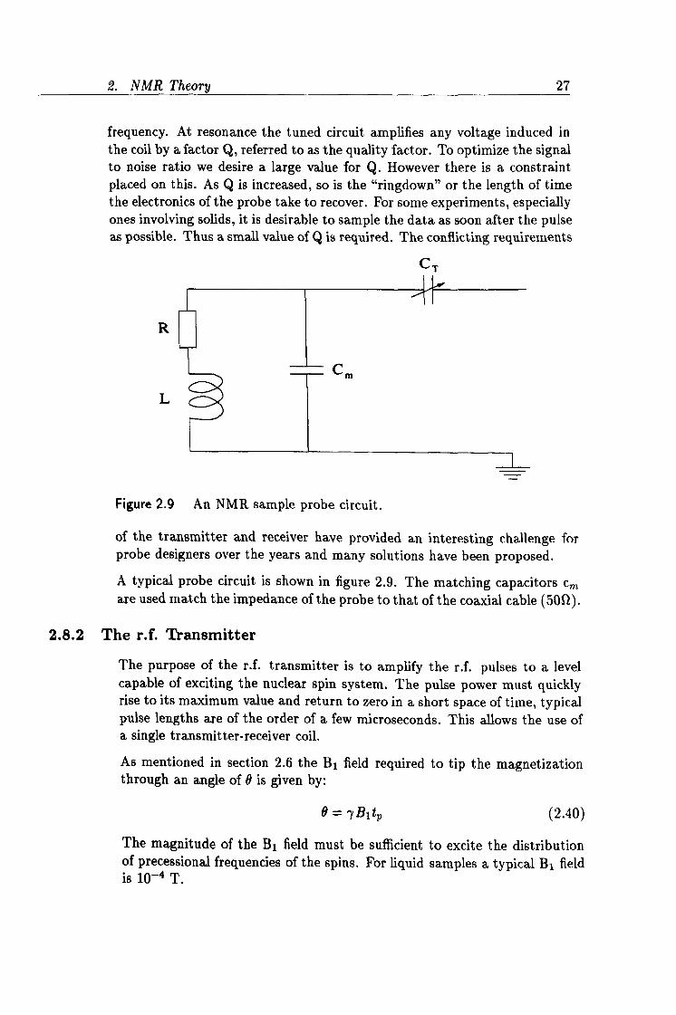
2.9 An NMR sample probe circuit. 27
3.1 The exponential form of the correlation function. 30
3.2 Plot of the spectral density. 31
3.3 Prediction of the BPP Theory. 33
3.4 Inversion recovery pulse sequence. 34
3.5 Hahn spin echo pulse sequence. 37
3.6 CPMG pulse sequence. 39
3.7 CONTIN output showing longitudinal relaxation distributions. 42
3.8 XFIT output showing T1 relaxation data. 44
3.9 XFIT output showing T2 relaxation data. 45
3.10 Experimental longitudinal relaxation curves of PAN solutions. 48
3.11 Arrhenius plot of Ti bow .
50
3.12 Arrhenius plot of T2 relaxation data. 52
iv
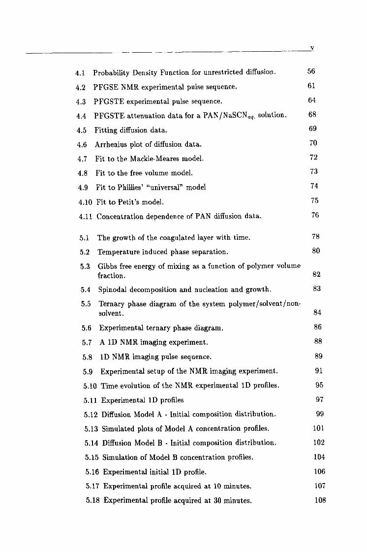
4.1 Probability Density Function for unrestricted diffusion. 56
4.2 PFGSE NMR experimental pulse sequence. 61
4.3 PFGSTE experimental pulse sequence. 64
4.4 PFGSTE attenuation data for a PAN/NaSCNa, q. solution. 68
4.5 Fitting diffusion data. 69
4.6 Arrhenius plot of diffusion data. 70
4.7 Fit to the Mackie-Meares model. 72
4.8 Fit to the free volume model. 73
4.9 Fit to Phillies' "universal" model 74
4.10 Fit to Petit's model. 75
4.11 Concentration dependence of PAN diffusion data. 76
5.1 The growth of the coagulated layer with time. 78
5.2 Temperature induced phase separation. 80
5.3 Gibbs free energy of mixing as a function of polymer volume fraction. 82
5.4 Spinodal decomposition and nucleation and growth. 83
5.5 Ternary phase diagram of the system polymer/solvent/non- solvent. 84
5.6 Experimental ternary phase diagram. 86
5.7 A 1D NMR imaging experiment. 88
5.8 1D NMR imaging pulse sequence. 89
5.9 Experimental setup of the NMR imaging experiment. 91
5.10 Time evolution of the NMR experimental ID profiles. 95
5.11 Experimental 1D profiles 97
5.12 Diffusion Model A- Initial composition distribution. 99
5.13 Simulated plots of Model A concentration profiles. 101
5.14 Diffusion Model B- Initial composition distribution. 102
5.15 Simulation of Model B concentration profiles. 104
5.16 Experimental initial 1D profile. 106
5.17 Experimental profile acquired at 10 minutes. 107
5.18 Experimental profile acquired at 30 minutes. 108
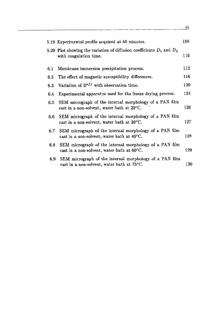
5.19 Experimental profile acquired at 60 minutes. 108
5.20 Plot showing the variation of diffusion coefficients D1 and D2
with coagulation time. 110
6.1 Membrane immersion precipitation process. 112
6.2 The effect of magnetic susceptibility differences. 116
6.3 Variation of Del f with observation time. 120
6.4 Experimental apparatus used for the freeze drying process. 124
6.5 SEM micrograph of the internal morphology of a PAN film cast in a non-solvent, water bath at 20°C. 126
6.6 SEM micrograph of the internal morphology of a PAN film
cast in a non-solvent, water bath at 30°C. 127
6.7 SEM micrograph of the internal morphology of a PAN film
cast in a non-solvent, water bath at 40°C. 128
6.8 SEM micrograph of the internal morphology of a PAN film cast in a non-solvent, water bath at 60°C. 129
6.9 SEM micrograph of the internal morphology of a PAN film cast in a non-solvent, water bath at 75°C. 130
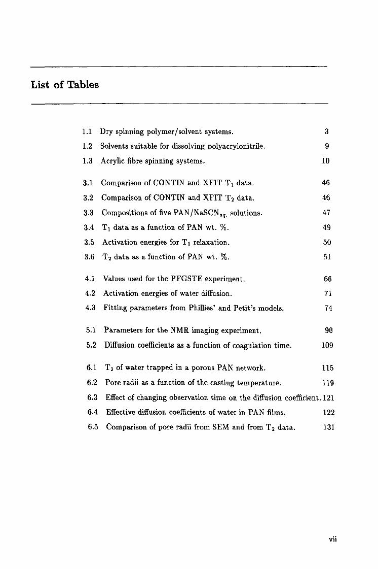
List of Tables
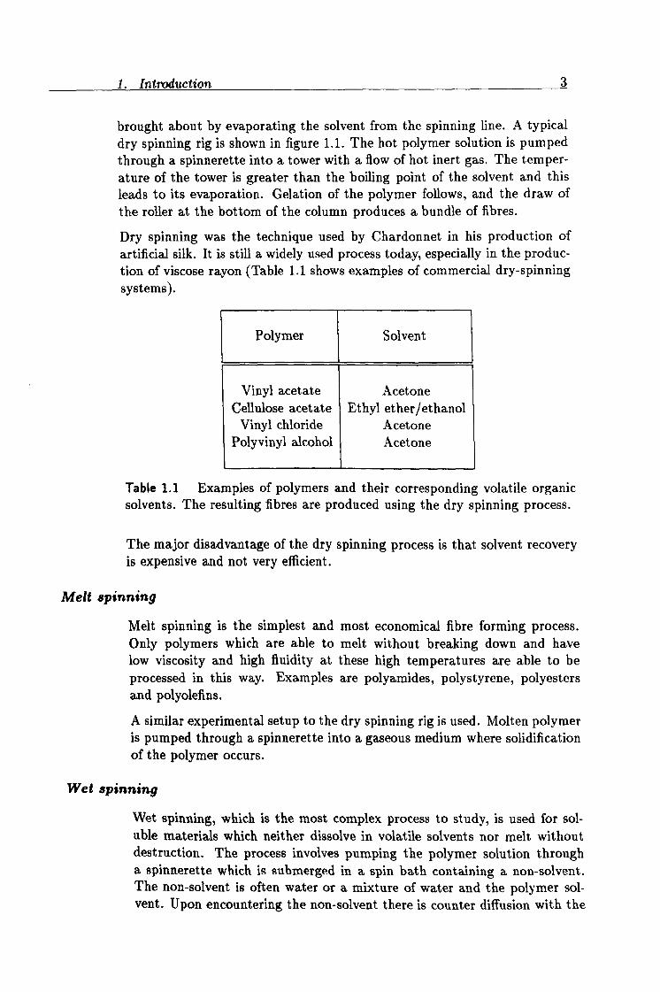
1.1 Dry spinning polymer/solvent systems. 3
1.2 Solvents suitable for dissolving polyacrylonitrile. 9
1.3 Acrylic fibre spinning systems. 10
3.1 Comparison of CONTIN and XFIT Tl data. 46
3.2 Comparison of CONTIN and XFIT T2 data. 46
3.3 Compositions of five PAN/NaSCNa, q. solutions. 47
3.4 T1 data as a function of PAN wt. %. 49
3.5 Activation energies for T1 relaxation. 50
3.6 T2 data as a function of PAN wt. %. 51
4.1 Values used for the PFGSTE experiment. 66
4.2 Activation energies of water diffusion. 71
4.3 Fitting parameters from Phillies' and Petit's models. 74
5.1 Parameters for the NMR imaging experiment. 90
5.2 Diffusion coefficients as a function of coagulation time. 109
6.1 T2 of water trapped in a porous PAN network. 115
6.2 Pore radii as a function of the casting temperature. 119
6.3 Effect of changing observation time on the diffusion coefficient. 121
6.4 Effective diffusion coefficients of water in PAN films. 122
6.5 Comparison of pore radii from SEM and from T2 data. 131
vii
viii
Abstract
The aim of the thesis was to study the phase behaviour of aqueous poly- acrylonitrile/NaSCN solutions using a variety of nuclear magnetic resonance techniques. Polyacrylonitrile (PAN) is the basis of the acrylic fibre industry, as such fibres contain at least 85% PAN. Despite this industrial importance, the available literature describing the phase behaviour of PAN in solution is far from comprehensive.
Bulk 1H NMR relaxation measurements were carried out over a wide range of concentrations and temperatures to probe the molecular dynamics of the PAN and water molecules. Both the T1 and T2 relaxation data was found to be bi-exponential decay for all samples, the relative amplitudes of which were shown to be equal to the ratio of PAN protons to water protons. Both species were found to be in the regime of rapid molecular motion.
Bulk 1H NMR self diffusion measurements, using the PFGSTE technique, exhibited a bi-exponential decay of the echo amplitudes. By careful selec- tion of the observation time, A, it was possible to independently probe the water and PAN translational diffusion. A background gradient, resulting from inhomogeneities of the magnetic field, complicated the analysis of the data and a novel polynomial least squares fitting procedure was devised to overcome this effect. The measured attenuation of the water diffusion co- efficients (D-10-6-10-5cm2s-1) with increasing PAN volume fraction was modelled according to various theories, including free volume and scaling laws. The study of the PAN diffusion coefficient (DN10-? -10 -6cm2s-1) was limited by the experimental constraints of the NMR spectrometer.
A 1H NMR one-dimensional imaging technique was used to study the non- solvent induced phase separation(coagulation) of a PAN solution. The time dependence of the measured profiles allowed observation of the coagulation process. A diffusion model was developed to fit the experimental data using a semi-infinite diffusion framework. The fitting parameters represented the diffusion coefficients of the water molecules in the solution/ coagulated PAN network, and in the bulk non-solvent/solvent. PAN films were cast at a range of temperatures in non-solvent baths. This was a scaling up of the dimensions of the fibre spinning process and was used to investigate the range of morphologies which can be formed in the wet-spinning of acrylic fibres. Before any drying processes, water molecules were confined in the porous structure of the saturated films, and their NMR relaxation and self diffusion behaviour was investigated. Parameters de- scribing the pore size and the tortuosity were derived from these studies and scanning electron microscopy was used as a comparative technique. The pore sizes predicted from the NMR data span a smaller spatial range than those observed from SEM. This is explained by the fundamental differences between the two techniques.
Acknowledgements
I would like to thank everyone who encouraged me throughout my time as a research student and made this thesis possible. Firstly my supervisor, Professor Ken Packer, for his continuous enthusiasm, guidance and advice. Thanks to Roger Ibbett and Courtaulds for interesting discussions and also for providing financial assistance.
Thanks to all the members of the NMR research group who made my time in the lab so satisfying. Special mentions to Bobby Damion for his immense mathematical powers, Dr. Jean for his incomprehensible Ingleesh, Pierre for proving the French have a sense of humour, and everyone else who I've had the pleasure of sharing an office with. Thanks also to all the other members of the Physical Chemistry Department who I've known through the years.
Special thanks to Sarah for her encouragement and tolerance, and for always being fun to be with.
Cheers to all the Wordsworth boys. Damo, Jim, Bridgey, Tristan, Smiffy, Skezza and Frank. It was a pleasure sharing the delights of Radford with you all.
Thanks to all the lads form the Lincoln and FCFC football teams. My seven years at Nottingham University were greatly enhanced by "the crack", both on and off the pitch.
Final thanks go to my parents for their continual moral and financial support, and encouragement. Without them none of this would have been possible.
Chapter 1 Introduction
1.1 Aims of the thesis The aim of the thesis is to study the phase behaviour of aqueous poly- acrylonitrile/NaSCN solutions using a variety of nuclear magnetic resonance techniques. This particular system has vast commercial importance in the acrylic fibre industry, where the phase separation of the polymer from solu- tion is induced by solvent/non-solvent counter diffusion.
The rest of this introductory chapter will describe the commercial relevance of the polyacrylonitrile system being studied, and a brief history of the syn- thetic fibre business will be given. The various industrial techniques used to produce fibres will be reviewed, along with a more detailed description of the wet spinning process. The physical properties of polyacrylonitrile, both in the solid and the solution state, will be discussed and the experimental studies of its phase behaviour will be reviewed.
Nuclear magnetic resonance techniques were used to acquire the bulk of the data presented in this thesis, therefore in order to understand these studies chapter 2 deals with the relevant NMR theory.
Chapter 3 and 4 cover the bulk NMR properties of aqueous polyacryloni- trile/NaSCN solutions over a wide range of temperatures and concentrations. The longitudinal and transverse relaxation studies provide information re- garding the dynamics of both the polymer and solvent molecules. The results are related to the classic B. P. P. theory [1]. The self diffusion studies of the solvent water molecules are modelled using a variety of proposed theories, ranging from free volume models first applied to polymer systems by Fu- jita in 1961 [2], to more recent paradigms, such as the "Universal" model proposed by Phillies [3].
The non-solvent induced phase separation of polyacrylonitrile is investigated in chapter 5 using a one dimensional NMR imaging technique. This dy- namic process is studied by monitoring the spatial concentration of solvent molecules as a function of experiment time. As the phase of the polyacry- lonitrile is determined by the composition of the solvent/non-solvent in the system, this approach allows one to analyse the process in terms of diffusion models. Chapter 6 studies saturated polyacrylonitrile cast films, by investigating the water confined in the porous polymer network. From the NMR data it is possible to estimate the pore sizes present in the film and these were compared to scanning electron micrographs of freeze dried films.
I
1. Introduction 2
Finally, chapter 7 concludes the thesis by summarising the interpretations of the work described in the rest of the tome.
1.2 Background The man-made fibre industry is a multi million pound business, in which the fibres are produced mainly for the production of textiles and woven products. It dates back to the 1930's when the first wholly synthetic fibres, polyvinyl chloride and polyamide were produced. The industry developed rapidly and by the 1950's there were over fifty different types of commercial man-made fibre available. In these early days the technology grew without any great knowledge of the underlying theoretical principles. This empirical knowledge gradually became augmented with more fundamental chemical studies. Indeed the generation of fibre technologists in the early twenti- eth century believed that fibre properties could be controlled solely by the chemical structure of the polymer material. From the 1960's the polymer physics of fibres has been developed and a more physical grounding in areas such as phase transitions and multicomponent heat and mass transfer is now available [41.
One of the most important group of synthetic fibres are acrylics. Acrylic fibres have a market share of about 20% of the worldwide production of man-made fibres [5]. Despite this large volume production and their history dating back to the 1930's, the polymer physics involved in the fibre formation is not fully understood.
The historical aspects of the production of acrylic and other synthetic fibres can be traced to the work of Chardonnet on cellulosics in the mid 1850's. He nitrated raw cotton to produce cellulose nitrate and then dissolved this in an ethyl ether/ethyl alcohol solvent to make a viscous solution, known as a "dope". The dope was fired through a spinnerette, which is a nozzle containing lots of tiny holes, to form fibres of cellulose nitrate. The fibres were washed, stretched and denitrified to produce the final product. Many important principles were used by Chardonnet in his pioneering work and the modern day industrial process of fibre spinning has many parallels to this early work. There are three main processes used to spin fibres. The one used by Chardon- net was dry spinning. The others are melt spinning, and wet spinning, which is used in the production of acrylic fibres and which we will concentrate on.
1.3 Fibre Spinning processes Dry Spinning
Solution dry spinning is used in the case of polymers which can be dissolved in volatile, usually organic, solvents. The phase separation of the "dope" is
1. Introduction 3
brought about by evaporating the solvent from the spinning line. A typical dry spinning rig is shown in figure 1.1. The hot polymer solution is pumped through a spinnerette into a tower with a flow of hot inert gas. The temper- ature of the tower is greater than the boiling point of the solvent and this leads to its evaporation. Gelation of the polymer follows, and the draw of the roller at the bottom of the column produces a bundle of fibres.
Dry spinning was the technique used by Chardonnet in his production of artificial silk. It is still a widely used process today, especially in the produc- tion of viscose rayon (Table 1.1 shows examples of commercial dry-spinning
systems).
Polymer Solvent
Vinyl acetate Acetone Cellulose acetate Ethyl ether/ethanol
Vinyl chloride Acetone Polyvinyl alcohol Acetone
Table 1.1 Examples of polymers and their corresponding volatile organic solvents. The resulting fibres are produced using the dry spinning process.
The major disadvantage of the dry spinning process is that solvent recovery is expensive and not very efficient.
Melt spinning
Melt spinning is the simplest and most economical fibre forming process. Only polymers which are able to melt without breaking down and have low viscosity and high fluidity at these high temperatures are able to be
processed in this way. Examples are polyamides, polystyrene, polyesters and polyolefins.
A similar experimental setup to the dry spinning rig is used. Molten polymer is pumped through a spinnerette into a gaseous medium where solidification of the polymer occurs.
Wet spinning
Wet spinning, which is the most complex process to study, is used for sol- uble materials which neither dissolve in volatile solvents nor melt without destruction. The process involves pumping the polymer solution through a spinnerette which is submerged in a spin bath containing a non-solvent. The non-solvent is often water or a mixture of water and the polymer sol- vent. Upon encountering the non-solvent there is counter diffusion with the
1. Introduction 4
Polymer Solution
Pump
Spinnerette
Heated
gas inlets
Jacketed cell
Gas to ". -' solvent 5;. recovery
III
to First roll 1(
To further processing
Figure 1.1 Schematic of a typical dry spinning tower.
solvent diffusing out of the polymer solution and the non-solvent diffusing in. This results in solidification of the fibre due to phase separation. The process is called coagulation.
The properties of the fibres produced using the wet spinning process are highly dependent on a number of factors, such as the "dope" composition, spin-bath temperature, spin-bath composition, etc. The parameters are care- fully selected to produce fibres of the required quality. If the conditions are not correct it is possible that unwanted structural features are introduced on the microscopic scale, such as large voids and capillaries, irregular shape of cross-sections and radially differentiated structure, and there may also be heterogeneity on the sub-micron scale. Much of the literature available concerning the formation of fibre structure, its relationship to the wet spinning variables and ultimately to the final properties of the fibre, is descriptive rather than analytical. The reported results tend to be inconsistent for different polymer/solvent systems and sometimes even for the same system. In the following section the background of the polyacrylonitrile system will be reviewed and the major trends of the spinning process noted. First some of the more general factors determining
1. Introduction 5
Polymer solution
0
Pump
Fresh non-solvent
Gui
Solvent recover;
SPIN BATH
Spinnerette
Figure 1.2 Schematic of a horizontal wet-spinning system.
fibre quality, and what effect they have, will be remarked upon.
" Polymer content in the "dope". A high polymer content tends to increase the polymer density in the fibre and thereby reduces the concentration of large voids and capil- laries. This leads to the production of a more homogeneous fibre. It is often impractical to work at high polymer concentrations. The viscosity will be large in these situations and will therefore demand high pressures to force the dope through the spinnerette. Also as the polymer concentration is increased the polymer solubility limit will be approached leading to phase separation.
" Solvent used. Each solvent type used dictates a characteristic fibre structure which is related to the interactions between the solvent and the polymer.
" Composition of spin bath. This can affect the cross-sectional shape of the fibre. The net flux of the solvent and non-solvent at the fibre surface may not be equal leading to irregularly shaped fibres, e. g. dog-bone shaped.
" Temperature of spin bath. Higher spin bath temperatures cause the cross-section of wet-spun fi- bres to become more circular. At these higher temperatures it is more likely that large voids may be formed so an intermediate temperature is usually selected [61
" Spin-draw ratio. The spin-draw ratio, or jet-stretch ratio as it is also known, is defined
Processing
1. Introduction 6
as the ratio of the rate at which protofibres are taken out of the coag- ulation bath, to the linear rate at which dope is pumped through the spinnerette holes. This parameter affects the orientation of the fibre
which leaves the spin bath.
The most important principles dictating the above parameters and the fibre structure are: (i) The relative diffusion rates of the solvent and non-solvent (ii) The phase separation characteristics of the ternary polymer/solvent/non- solvent system. The slower the coagulation rate, the more dense and fine the fibre structure becomes. This leads to improvements in the mechanical properties such as tensile strength and modulus [7].
Post-spinning treatments
All wet spinning processes use further washing and orientation processes after coagulation in the spin bath. These remove excess solvent remaining in the fibre and develop internal fibre morphology for greater strength.
" Washing. Fibre washing, being a difusional process, is driven by the concentra- tion of the wash liquid and by temperature. At this stage the fibre structure is still porous and additives such as dyes can be incorpo- rated here. Commercial acrylic fibres are normally washed with water at temperatures in the region of the wash liquids boiling temperature.
" Fibre drawing. The drawing process increases the orientation of the fibre and thereby increases its strength. The fibre is stretched up to twelve times its length at high temperatures, using hot water and a set of rollers.
" Finish. The finishing step usually involves applying a chemical treatment to the fibre. This is normally an aqueous solution containing lubricants and anti-static components. The "finish" is applied to aid processing in the collapse/drying stage and to allow transformation of the fibre into yarns.
" Drying, collapsing, relaxing. These stages, normally applied simultaneously, involve removing the remaining water from the internal fibrillar network in order to close the open pore structure. The fibre temperature is normally increased to the wet glass transition temperature [8].
1. Introduction 7
1.4 Polyacrylonitrile
1.4.1 Structure
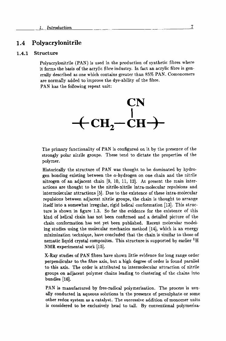
Polyacrylonitrile (PAN) is used in the production of synthetic fibres where it forms the basis of the acrylic fibre industry. In fact an acrylic fibre is gen- erally described as one which contains greater than 85% PAN. Comonomers are normally added to improve the dye-ability of the fibre. PAN has the following repeat unit:
CN
ýCHZ CH--)-
The primary functionality of PAN is configured on it by the presence of the strongly polar nitrile groups. These tend to dictate the properties of the polymer.
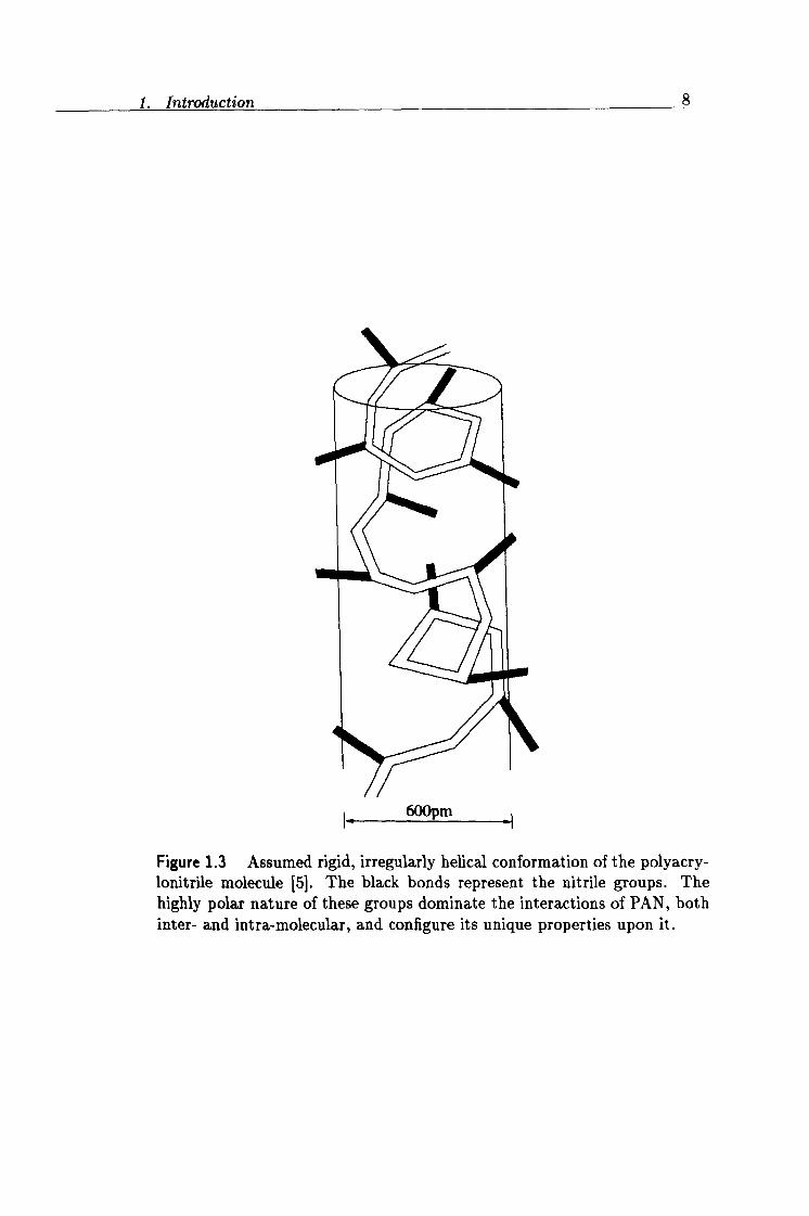
Historically the structure of PAN was thought to be dominated by hydro- gen bonding existing between the a-hydrogen on one chain and the nitrile nitrogen of an adjacent chain [9,10,11,12]. At present the main inter- actions are thought to be the nitrile-nitrile intra-molecular repulsions and intermolecular attractions [5]. Due to the existence of these intra-molecular repulsions between adjacent nitrile groups, the chain is thought to arrange itself into a somewhat irregular, rigid helical conformation [13]. This struc- ture is shown in figure 1.3. So far the evidence for the existence of this kind of helical chain has not been confirmed and a detailed picture of the chain conformation has not yet been published. Recent molecular model- ing studies using the molecular mechanics method [14], which is an energy minimization technique, have concluded that the chain is similar to those of nematic liquid crystal composites. This structure is supported by earlier 1H NMR experimental work [15].
X-Ray studies of PAN fibres have shown little evidence for long range order perpendicular to the fibre axis, but a high degree of order is found parallel to this axis. The order is attributed to intermolecular attraction of nitrile groups on adjacent polymer chains leading to clustering of the chains into bundles [16].
PAN is manufactured by free-radical polymerisation. The process is usu- ally conducted in aqueous solutions in the presence of persulphate or some other redox system as a catalyst. The successive addition of monomer units is considered to be exclusively head to tail. By conventional polymerisa-
1. Introduction 8
Figure 1.3 Assumed rigid, irregularly helical conformation of the polyacry- lonitrile molecule [5]. The black bonds represent the nitrile groups. The highly polar nature of these groups dominate the interactions of PAN, both inter- and intra-molecular, and configure its unique properties upon it.
pm
1. Introduction 9
tion techniques PAN forms both isotactic and syndiotactic configurations in
approximately equal proportion, making PAN atactic in nature [17,181.
It is rare for such atactic polymers to show a high degree of crystallinity, but PAN demonstrates a significant amount of order of about 30% [19]. The
nature of this crystallinity is still the subject of some discussion [20].
1.4.2 Solvents and the solution state of PAN
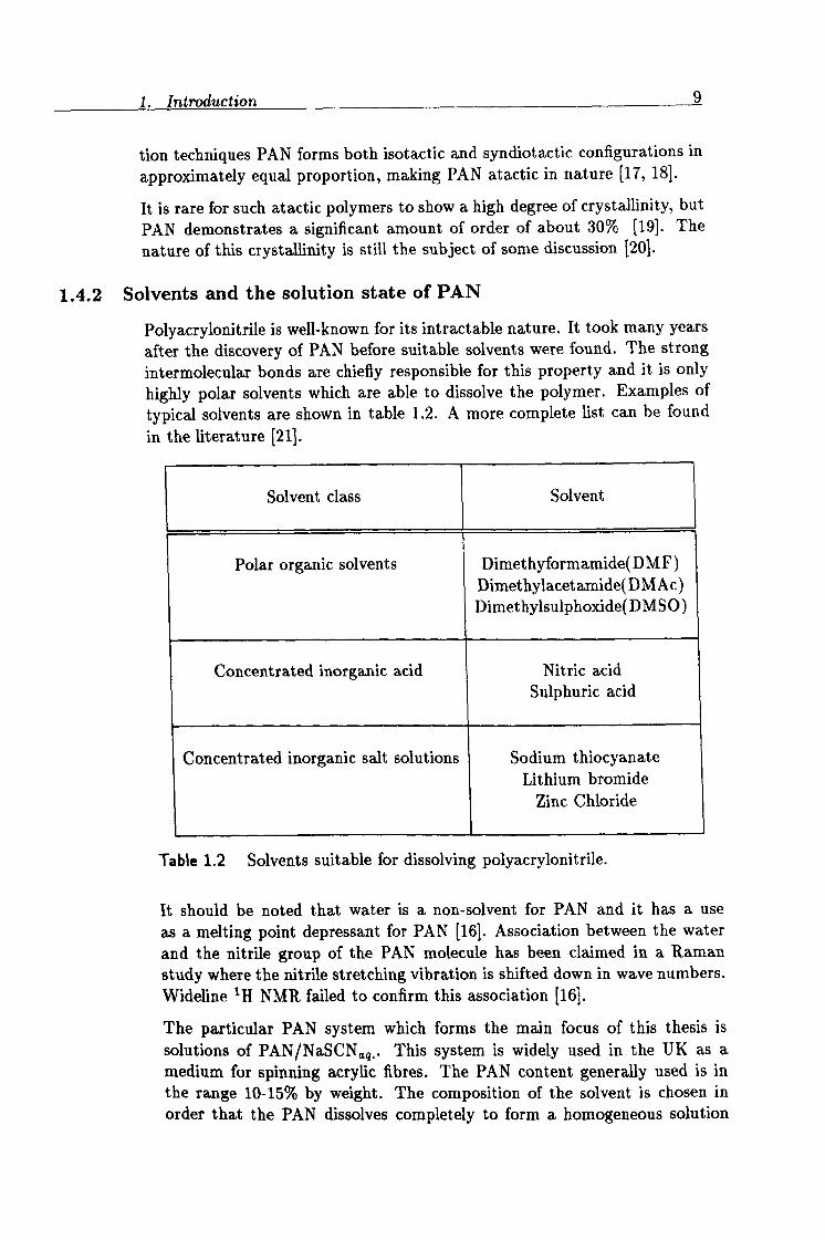
Polyacrylonitrile is well-known for its intractable nature. It took many years after the discovery of PAN before suitable solvents were found. The strong intermolecular bonds are chiefly responsible for this property and it is only highly polar solvents which are able to dissolve the polymer. Examples of typical solvents are shown in table 1.2. A more complete list can be found in the literature [21].
Solvent class Solvent
Polar organic solvents Dimethyformamide(DMF) Dimethylacetamide(DMAc) Dimethylsulphoxide(DMSO)
Concentrated inorganic acid Nitric acid Sulphuric acid
Concentrated inorganic salt solutions Sodium thiocyanate Lithium bromide
Zinc Chloride
Table 1.2 Solvents suitable for dissolving polyacrylonitrile.
It should be noted that water is a non-solvent for PAN and it has a use as a melting point depressant for PAN [16]. Association between the water and the nitrile group of the PAN molecule has been claimed in a Raman
study where the nitrile stretching vibration is shifted down in wave numbers. Wideline 1H NMR failed to confirm this association [161.
The particular PAN system which forms the main focus of this thesis is solutions of PAN/NaSCNaq,. This system is widely used in the UK as a medium for spinning acrylic fibres. The PAN content generally used is in the range 10-15% by weight. The composition of the solvent is chosen in order that the PAN dissolves completely to form a homogeneous solution
1. Introduction 10
and so that the dope viscosity is at a minimum. This is normally in the range 45-70% by weight NaSCN. For a 10% PAN solution this occurs at a NaSCN concentration of 50% by weight [22].
The exact mechanism for the dissolution of PAN in inorganic salts is not fully understood. Using viscosity studies Geller [22] speculated that there will be interaction between the nitrile group of PAN with the solvation layer of the NaSCN salt. Infra-red spectroscopic studies [23] have indicted that no complexation occurs between the nitrile groups and sodium cations when ei- ther PAN-co-vinyl acetate or acetonitrile were dissolved in aqueous sodium thiocyanate. More recent work [24], using Raman spectroscopy, has sug- gested that the ability of aqueous NaSCN solutions to dissolve PAN can be
attributed to the water structure breaking qualities of thiocyanate anions. The non-hydrogen bonded bands are seen to be enhanced by the addition of certain anions, including thiocyanate, indicating break-up of the water struc- ture. This enables the water molecules to interact with the highly polarized nitrile groups of PAN.
The dissolved state of PAN in polar organic solvents, such as DMF and DMAc, appears to be more clearly defined in a paper by Hattori et al. [251. The organic solvent molecules form 7r-electron conjugate systems with the orbitals of the PAN nitrile groups. The same paper also mentions aqueous NaSCN as being a solvent for PAN, but as the solvent structure itself is not clear, discussion of its interaction with PAN is limited.
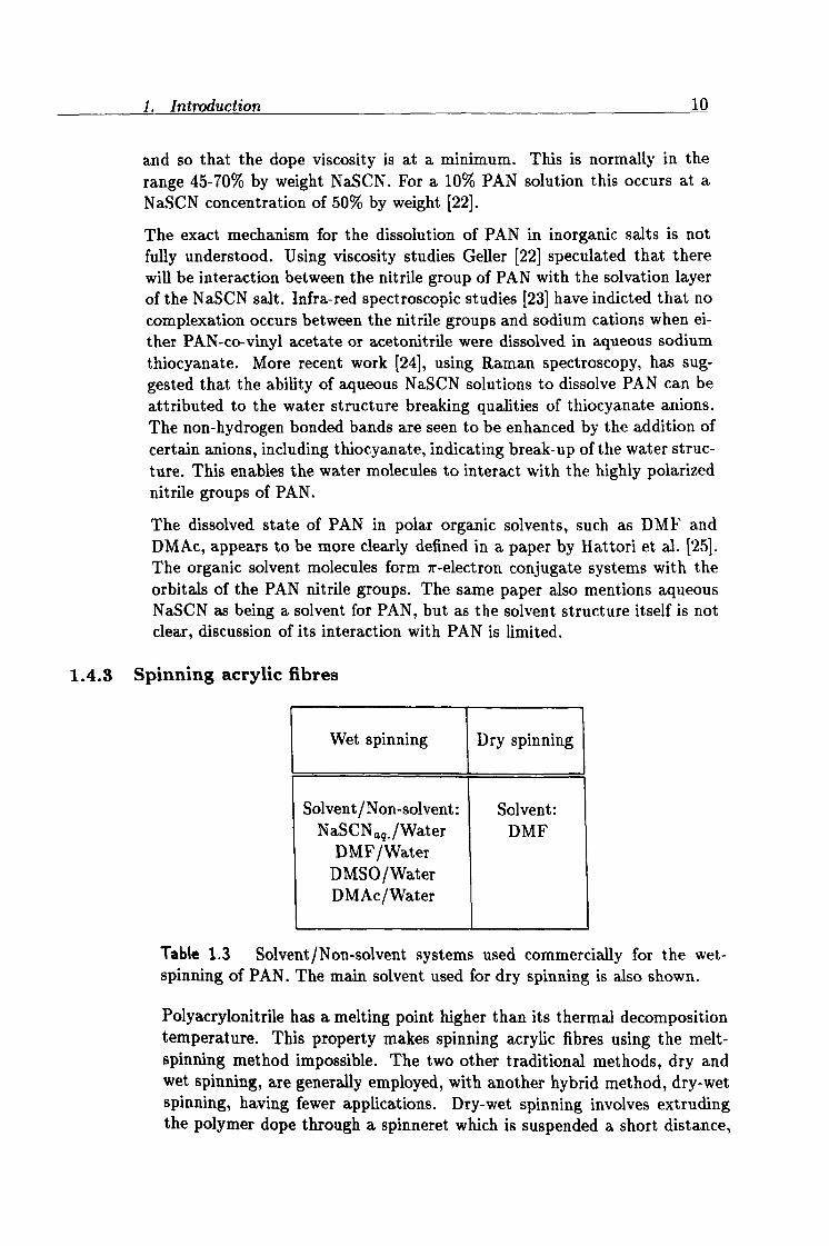
1.4.3 Spinning acrylic fibres
Wet spinning Dry spinning
Solvent/Non-solvent: Solvent: NaSCNa, q. /Water DMF
DMF/Water DMSO/Water DMAc/Water
Table 1.3 Solvent/Non-solvent systems used commercially for the wet- spinning of PAN. The main solvent used for dry spinning is also shown.
Polyacrylonitrile has a melting point higher than its thermal decomposition temperature. This property makes spinning acrylic fibres using the melt- spinning method impossible. The two other traditional methods, dry and wet spinning, are generally employed, with another hybrid method, dry-wet spinning, having fewer applications. Dry-wet spinning involves extruding the polymer dope through a spinneret which is suspended a short distance,
1. Introduction 11
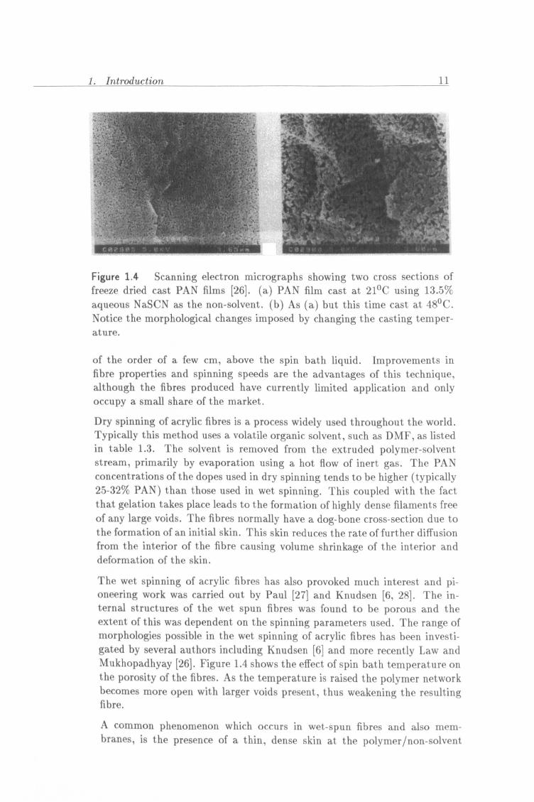
Figure 1.4 Scanning electron micrographs showing two cross sections of freeze dried cast PAN films [26]. (a) PAN film cast at 21°C using 13.5%
aqueous NaSCN as the non-solvent. (b) As (a) but this time cast at 48°C. Notice the morphological changes imposed by changing the casting temper-
ature.
of the order of a few cm, above the spin bath liquid. Improvements in fibre properties and spinning speeds are the advantages of this technique, although the fibres produced have currently limited application and only occupy a small share of the market. Dry spinning of acrylic fibres is a process widely used throughout the world. Typically this method uses a volatile organic solvent, such as DMF, as listed in table 1.3. The solvent is removed from the extruded polymer-solvent stream, primarily by evaporation using a hot flow of inert gas. The PAN concentrations of the dopes used in dry spinning tends to be higher (typically 25-32% PAN) than those used in wet spinning. This coupled with the fact that gelation takes place leads to the formation of highly dense filaments free of any large voids. The fibres normally have a dog-bone cross-section due to the formation of an initial skin. This skin reduces the rate of further diffusion from the interior of the fibre causing volume shrinkage of the interior and deformation of the skin.
The wet spinning of acrylic fibres has also provoked much interest and pi- oneering work was carried out by Paul [27] and Knudsen [6,28]. The in- ternal structures of the wet spun fibres was found to be porous and the extent of this was dependent on the spinning parameters used. The range of morphologies possible in the wet spinning of acrylic fibres has been investi- gated by several authors including Knudsen [6] and more recently Law and Mukhopadhyay [26]. Figure 1.4 shows the effect of spin bath temperature on the porosity of the fibres. As the temperature is raised the polymer network becomes more open with larger voids present, thus weakening the resulting fibre.
A common phenomenon which occurs in wet-spun fibres and also mem- branes, is the presence of a thin, dense skin at the polymer/non-solvent
Introduction 12
,.
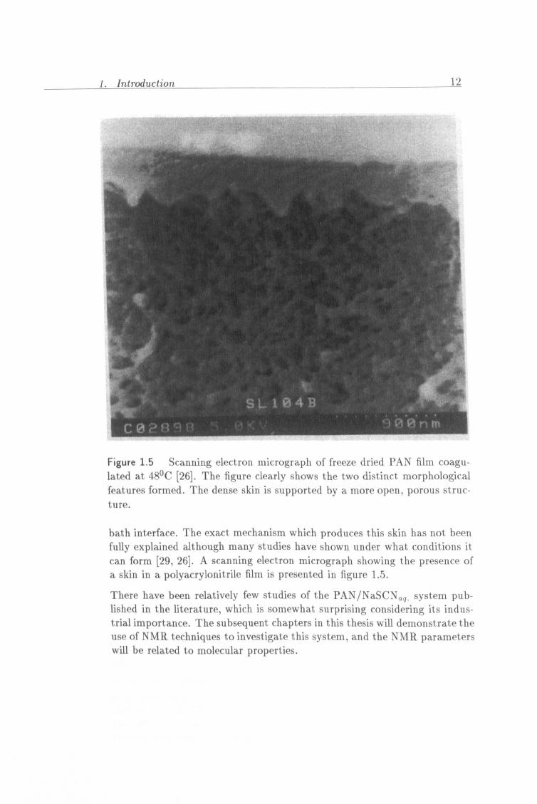
Figure 1.5 Scanning electron micrograph of freeze dried PAN film coagu- lated at 48'C [26]. The figure clearly shows the two distinct morphological features formed. The dense skin is supported by a more open, porous struc- ture.
bath interface. The exact mechanism which produces this skin has not been fully explained although many studies have shown under what conditions it can form [29,26]. A scanning electron micrograph showing the presence of a skin in a polyacrylonitrile film is presented in figure 1.5.
There have been relatively few studies of the PAN/NaSCNa, q. system pub- lished in the literature, which is somewhat surprising considering its indus- trial importance. The subsequent chapters in this thesis will demonstrate the use of NMR techniques to investigate this system, and the NMR parameters will be related to molecular properties.
Chapter 2 NMR Theory
2.1 Introduction This chapter introduces the principles of Nuclear Magnetic Resonance (NMR)
and in it the emphasis will be placed on explaining the concepts which will be used later in the thesis.
There are a plethora of excellent texts available on the fundamental theory of NMR. The books which proved useful in the writing of this chapter are by Harris [30], Slichter [31], Farrar and Becker [32]
, Cowan [33], and Hennel
and Klinowski [34]. More specific texts on the NMR of polymers in the solid and solution state, used in this thesis, are by McBrierty and Packer [35], and by Delpuech [361.
2.2 Background The history of NMR can be traced back to the development of spin as a fundamental quantum entity. Pauli is normally credited with the idea of nuclear spin as a means of explaining hyperfine spectral structure [37]. Cer- tain nuclei were found to have intrinsic angular momentum, and as with any spinning charge an associated magnetic moment.
The first observations of NMR in bulk materials were first reported by two independent research groups: Bloch, Hansen and Packard [38] working on the west coast of America at Stanford and Purcell, Torrey and Pound [39]
at Harvard on the east coast. They both published their initial findings in the same issue of Physical review in 1946 and shared the Nobel prize in 1952 "for the development of new methods for nuclear magnetic precession measurements and discoveries therewith".
Almost all of the pioneering NMR experiments were carried out using a continuous wave (CW) method. The idea of pulsed NMR was first suggested by Bloch [40], but it was not fully exploited until a few years later. The most notable early contribution was undoubtedly the work of Hahn whose paper in 1950 [41] showed that the decay of the transverse magnetization caused by the effects of molecular diffusion in an inhomogeneous field could be refocused by a second r. f. pulse to form a `spin echo'.
In the 1950's NMR became quite a high profile research field for scientists other than physicists. The discovery of the chemical shift phenomenon and high resolution NMR, made the subject useful to chemists as an analytical tool for structural elucidation. The most noteworthy early paper demon- strating this application was by Arnold, Dharmatti and Packard [42], who
13
2. NMR Theory 14
showed separate lines for chemically non-equivalent protons in ethanol.
The next major breakthrough came in the 1960's with the development
of the Fast Fourier Transform using the Cooley Tukey algorithm [43] to relate frequency and time. The relationship was first published by Lowe and Norberg in 1959 [44] when they related the FID and the slow passage spectrum of a solid. Later with the increasing availability of microcomputers Ernst and Anderson's paper [45] showed this application to be practical and advantageous, and led to the development of more advanced commercial pulsed NMR spectrometers.
The use of applied field gradients was not an unknown concept when Stejskal and Tanner published their paper in 1965. In fact the papers of Hahn [41]
and Carr and Purcell [46] formed the foundation for this work. Stejskal and Tanner [47] though used gradient pulses which allowed diffusion coefficients of less mobile species, such as polymers, to be measured.
The discovery of NMR Imaging by Lauterbur [48] in America and inde- pendently by Mansfield and Grannel [49] in Nottingham, England in 1973 caused a lot of excitement especially in the medical community. The first live human image was that of a human finger [50]. This was followed by that of a hand [51] and the advances in magnet design led to whole body systems being developed. Today MRI is used in hospitals throughout the world as an investigative technique alongside traditional methods such as X-Rays.
NMR has progressed amazingly in its first fifty years and nobody at the time of its discovery could have envisaged the importance and broad applications of its use.
2.3 Magnetic Moments The concept of a nucleus containing its own angular momentum and its own associated intrinsic magnetic moment goes back to the discoveries of Pauli in 1924 [371. This was several months before the introduction of electron `spin' by Uhlenbeck and Goudsmit [521. The introduction of nuclear `spin' helped to explain the ultra fine structure of atomic spectra. The magnetic moment for both entities was shown to be proportional to the intrinsic angular momentum.
µ=ryI (2.1)
where I is the spin angular momentum for a given nucleus. p is the magnetic moment. y is the magnetogyric ratio and is constant for a given nucleus. It takes the form of the following:
2m gne
(2.2) P
2. NMR Theory 15
where gar is the nuclear g factor or Lande factor. For the proton g,, = 5.5856912 mp is the mass of the proton. e is the charge of the proton.
We can see that the magnetic moment µ is dependent upon the spin angular momentum and the value of the Lande factor. Physicists spent the first years after the discovery of NMR measuring values of µ for a wide range of nuclei. These measurements were obviously limited to those nuclei having I>0.
There are some empirical rules available which determine the value of I. Nuclei with an even number of protons and neutrons have 1=0, e. g. 12C. These nuclei are NMR inactive. Nuclei which contain both an odd number of protons and an odd number of neutrons have an integer spin, e. g. 14N. Those with either an odd number of protons or an odd number of neutrons have a half integer spin, e. g. 1 H.
2.4 Nuclear Energy Levels If we consider a nucleus with magnetic moment it placed in a static magnetic field of strength Bo, arbitrarily along the z axis, there will be a interaction between the two which leads to the initially degenerate energy levels split- ting.
The energy of a magnetic moment is in a magnetic field Bo is given classically as -µ. Bo, or quantum mechanically the mth state is given as:
Em = -ymhBo (2.3)
where once again y is the magnetogyric ratio. m has 21+1 values ranging from -I through to +1.
The energy difference between two adjacent levels is given by:
DE = hyBo (2.4)
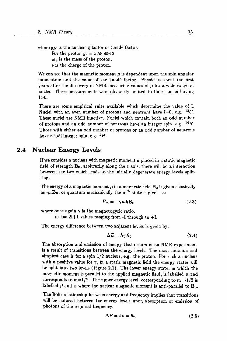
The absorption and emission of energy that occurs in an NMR experiment is a result of transitions between the energy levels. The most common and simplest case is for a spin 1/2 nucleus, e. g. the proton. For such a nucleus with a positive value for ry, in a static magnetic field the energy states will be split into two levels (Figure 2.1). The lower energy state, in which the magnetic moment is parallel to the applied magnetic field, is labelled a and corresponds to m=1/2. The upper energy level, corresponding to m=-1/2 is labelled /3 and is where the nuclear magnetic moment is anti-parallel to Bo.
The Bohr relationship between energy and frequency implies that transitions will be induced between the energy levels upon absorption or emission of photons of the required frequency.
DE = by = hw (2.5)
2. NMR
a
Figure 2.1 Zeeman nuclear energy levels.
16
w is the angular frequency in radians/second w= 27rv, where v is the reso- nant frequency in Hz.
By comparing this to equation 2.4 we can express the angular frequency required to induce transitions in terms of the applied magnetic field and the magnetogyric ratio.
V=0 (2.6) B
v is known as the Larmor frequency. More commonly it is expressed in terms of the angular frequency:
w= 'yB0 (2.7)
The number of particles per unit volume in each of the two states a and 0, referred to respectively as ̀ spin up' and `spin down', can be denoted as N, and Np. By Boltzmann's principle the ratio Na/NQ at thermal equilibrium is given by:
Na/Np = exp(DE/kT) (2.8)
where k is Boltzmann's constant and T is the absolute temperature. Substituting in equation: 2.4 we get:
Na/Np = exp(h7Bo/kT) (2.9)
At thermodynamic equilibrium, at normal temperatures, the population of the higher energy level is less than that of the lower energy level. This population difference is very small, for example for protons (-y = 26.75x10⁷ Tad' T-ls'1), at T=293K and Bo =1 Tesla, we find the population differ- ence is just seven in one million. This makes the NMR technique inherently insensitive.
2.5 Resonance Many aspects of NMR can be understood by using the energy level approach explained so far. Another method however proves to be more useful for
2. NMR Theory 17
Z
Y
A
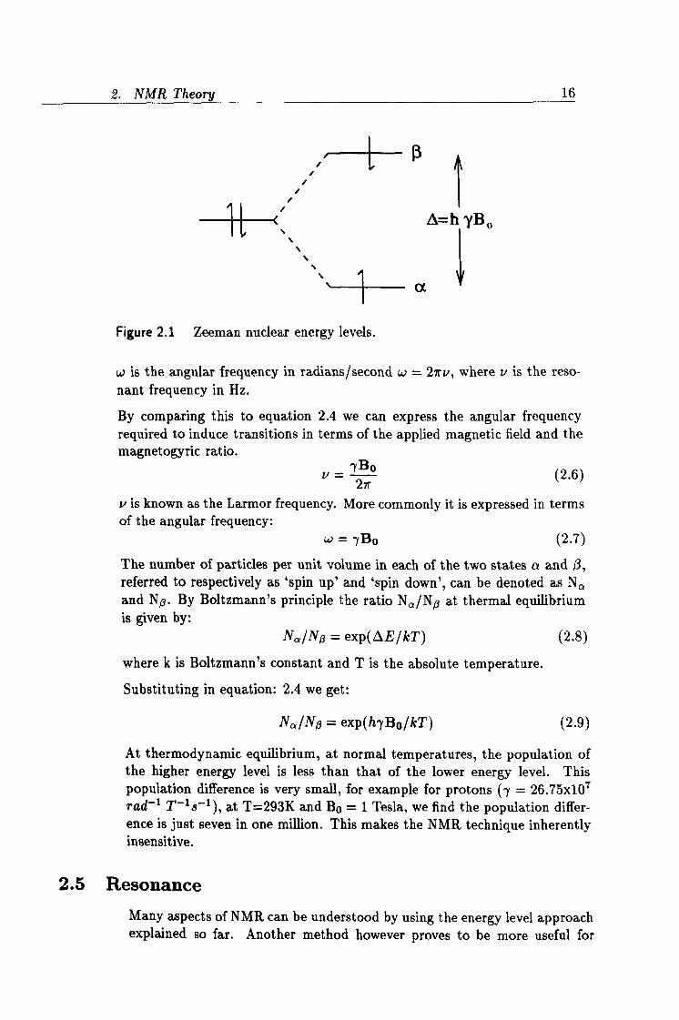
Figure 2.2 Precession of a magnetic moment about a static magnetic field Bo
visualizing the effects of the magnetic fields upon the magnetic moments. This approach uses a classical treatment and will prove useful in explaining the experiments outlined in this thesis.
2.5.1 Larmor Precession
The classical approach to NMR is based upon the precession of a magnetic moment µ, with angular momentum I, about an applied magnetic field Bo
with angular frequency:
w= -yBo (2.10)
The negative sign is used to illustrate a right hand corkscrew protocol. Figure 2.2 shows the direction of Larmor precession for positive magnetogyric ratio.
This precession occurs because the magnetic moment µ experiences a torque expressed by the rotational equivalent of Newton's Second Law:
T=µxBo (2.11)
The equation of motion for the system can be found by equating the torque to the rate of change of angular momentum:
dI dt_µxBo
(2.12)
but since µ= yI , we obtain:
dt = 7µ x Bo (2.13)
2. NMR Theory 18
Z
m=-1/2
m=+1/2
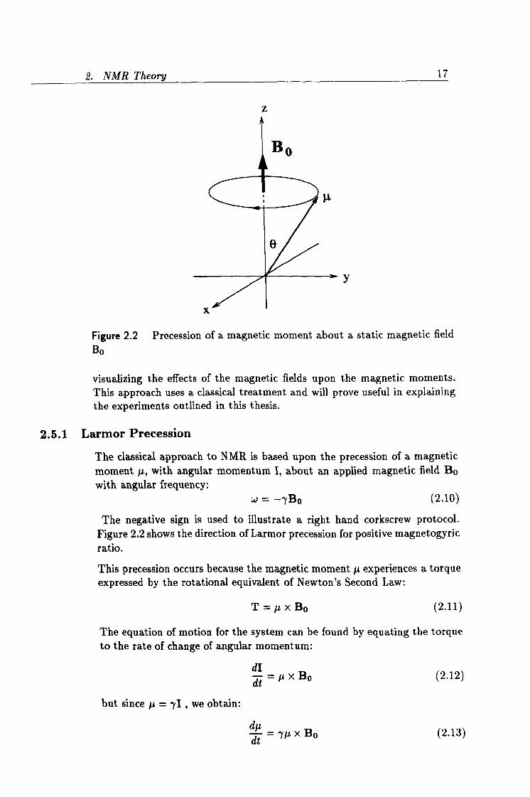
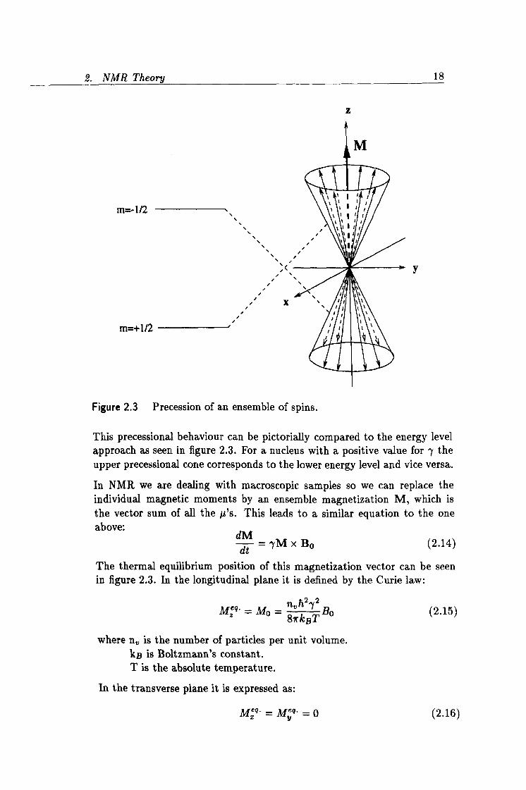
Figure 2.3 Precession of an ensemble of spins.
Y
This precessional behaviour can be pictorially compared to the energy level approach as seen in figure 2.3. For a nucleus with a positive value for y the upper precessional cone corresponds to the lower energy level and vice versa.
In NMR we are dealing with macroscopic samples so we can replace the individual magnetic moments by an ensemble magnetization M, which is the vector sum of all the µ's. This leads to a similar equation to the one above: dM
dt = yM x Bo (2.14)
The thermal equilibrium position of this magnetization vector can be seen in figure 2.3. In the longitudinal plane it is defined by the Curie law:
nh22 Mxq M0 = 8-rk T Bo (2.15)
where n� is the number of particles per unit volume. kB is Boltzmann's constant. T is the absolute temperature.
In the transverse plane it is expressed as:
Mxq = Mu"- =0 (2.16)
2.5.2
2.5.3
2. NMR
Radio-frequency Excitation
19
In an NMR experiment the excitation of spins from their equilibrium state is brought about by a second, oscillating magnetic field 2B1, which is per- pendicular to the static Bo field. This transverse magnetic field oscillates at wo, the Larmor frequency, and can be separated into two components, one rotating in the same sense as the magnetization (w) and the other in the
opposite direction (+w). We are only interested in -w as this produces the torque which rotates the magnetization into the xy plane:
(2.17) B1(t) = Bi coswoti - B1 sin wotj
The total field acting on the sample is then:
B= Bi cos woti - Bl sin wotj + Bok (2.18)
i, j and k are unit vectors along the x, y and z axes.
We can now write the equation of motion of the magnetization including the effects of the oscillating B1 field and also the static Bo field:
dM _µx1'[Bo+Bi(t)] dt
Rotating Frame of Reference
(2.19)
Conventionally the time dependence of the B1 field can be eliminated by introducing a rotating frame coordinate system, which rotates about Bo in the same direction as the magnetic moments precess. In such a system both B1 and Bo will be static, but there will be changes to the equations of motion.
Consider a vector M in terms of its components:
M= Mai + Myj + Mk (2.20)
Now consider its time derivative in a rotating frame of reference:
(dM = OMA aMz ai a; ak
WT (OM, ý,
at j + at + at k) + Mx
at + My at + Mz at (2.21)
The part of the equation in brackets is the the time derivative of the magne- tization in the rotating reference frame where i, j and k appear stationary.
Equation 2.21 can be expressed as:
or Cddt
)= at + wx (Mxi + Myj + Mk) (2.22)
dM _
äM }wXM (2.23) dt
stationary at
rotating
2. NMR Theory 20
Z'
w/y I
Bo
X'
B1
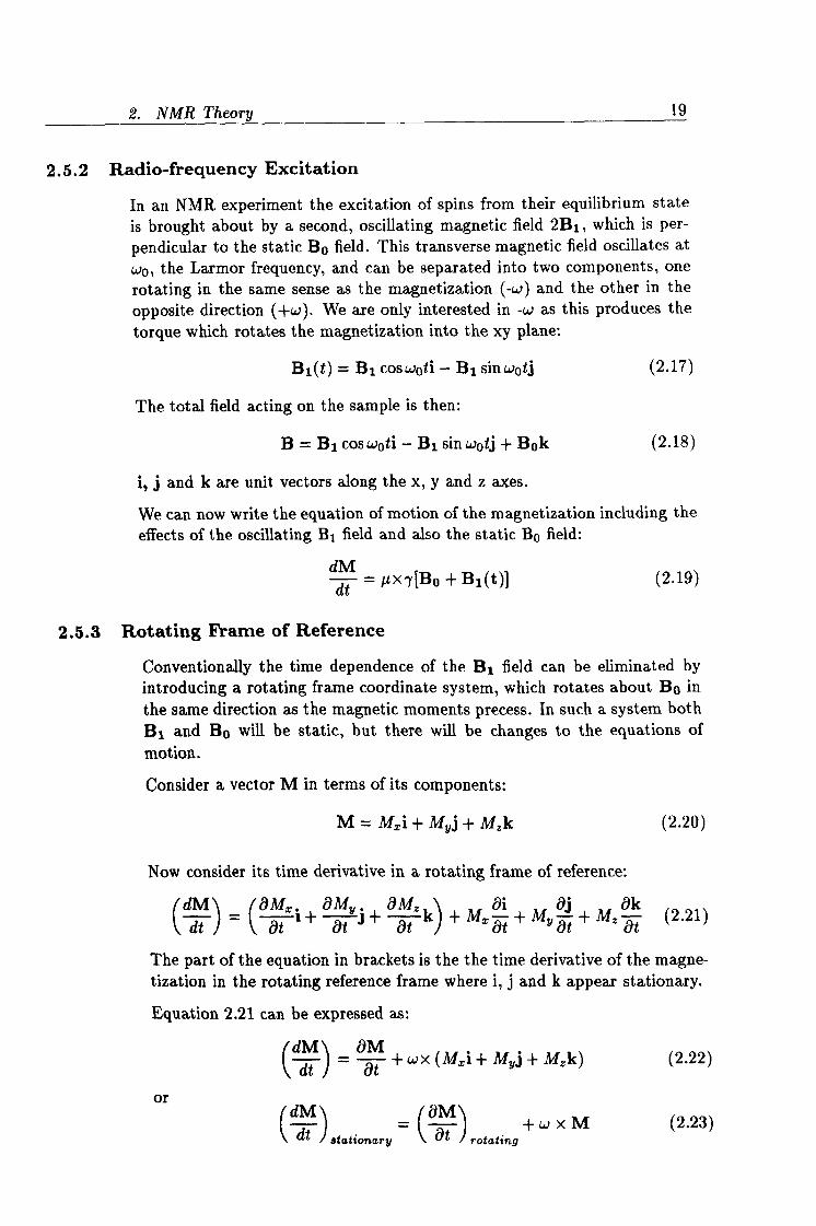
Figure 2.4 Effective magnetic field Bo
If M now represents the magnetization in a static magnetic field, we know from equation 2.14:
dM dt) = yM x Bo (2.24)
stationary
so from equation 2.23 we can now write:
am C at) = 1M x Bo-w xM (2.25) rotating
This is more commonly expressed as:
am) C at J= yM x Beff (2.26) l rotating
where: Bell = Bo +k (2.27)
\7/ Comparing equation 2.26 to equation 2.14 we see that the equation of motion in the rotating frame is the same as that in the laboratory frame, but with Bo replaced by Beff.
With the application of the B1 field, which rotates in the laboratory frame at an angular frequency -w, perpendicular to Bo, we find the effective field in the rotating frame is now:
Beff = BO + (w) k+ Bl (2.28)
7
2. NMR
F. T.
21
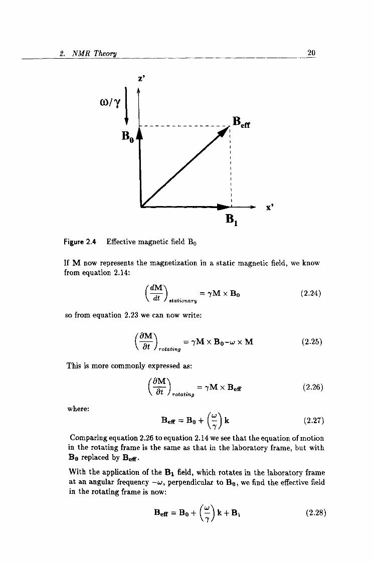
Figure 2.5 A r. f. pulse of length tp with its Fourier transform. The fre-
quency distribution is seen to be centred around the carrier frequency v,
The effective magnetic field can be illustrated as in figure 2.4. The magnetic moments precess with angular frequency yBe jf in a cone of fixed angle about Be f f. The quantity ry is often called the fictitious field, due to its
contribution to Be ff in the rotating frame of reference.
From equation 2.28 we can see that when the resonance condition is satisfied, i. e. w= --tBo, the effective field is simply the applied B1 field. The magnetic moments are tilted into towards the x-y plane where they will precess.
2.6 Pulse and Fourier NMR The pioneering NMR experiments were carried out in continuous wave (CW)
mode. This method involved slowly scanning the frequency range of interest during which resonance would be passed through with an absorption of en- ergy. These experiments were inherently slow and therefore signal to noise was low.
2.6.1 The Fourier Transform
In 1966 Ernst and Anderson's paper [451 introduced the use of pulse Fourier methods to acquire NMR spectra. High power r. f. pulses were used to excite the nuclei and a Fourier transform of the resulting free induction decay (FID) produced the spectrum. The introduction of this method along with the increasing availability of microcomputers made the pulse NMR experiment far more efficient than the CW method. Nowadays the majority of NMR experiments are carried out using a sequence of r. f. pulses and delays. These pulse programs allow complex manipulation of the spin system. Fourier analysis shows us that a short r. f. pulse will contain a range of frequencies centred on a frequency v, The distribution of these frequencies and their
-- tp
-º
2. NMR Theory 22
relationship to the pulse length tp can be seen in figure 2.5 and is given by:
P(v) = sin[r(v - v, )tpl (2.29)
r(v - v, )tp
The Fourier transformation is the mathematical relationship between the time domain and the frequency domain:
F(v) J +00
f (t) exp(-i2irvt)dt (2.30) 00
+00 f (t) =J F(v) exp(+i2avt)dt (2.31)
In practice Fourier transformation is carried out using the Cooley-Tukey
algorithm [43]. Using this method the integrals are taken over a finite time interval and the number of data points is restricted to 2n, where n is any integer.
2.6.2 Pulse experiments
In a pulse NMR experiment the magnetization vector, initially along the z-axis is tipped toward the x-y plane by the use of a short r. f. pulse B1. At the end of the pulse duration the magnetization will have been tipped through a flip angle given by:
0= yBitp (2.32)
Following a 90° pulse the magnetization vector will be in the x-y plane. The spins will be bunched or in other words will have phase coherence. After the pulse has been switched off the spins will start to relax back to their equilibrium values and will lose their phase coherence due to magnetic field inhomogeneity and transverse relaxation, the timescale of which is repre- sented generally by the transverse relaxation time T. If a receiver coil is
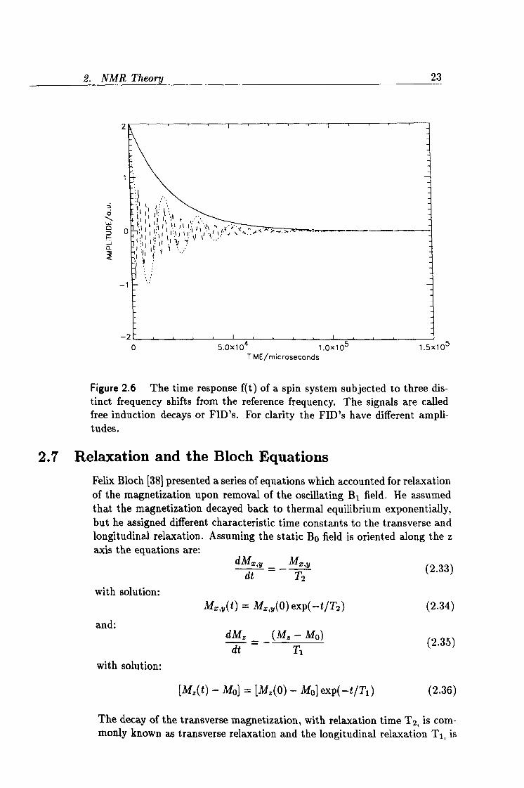
placed in the x-y plane then an voltage will be induced in the coil and an NMR signal will be detected. The magnetization is viewed in a rotating frame by feeding the reference Larmor frequency to the phase sensitive de- tector. The loss of phase coherence leads to an attenuation of this signal. A plot of the signal amplitude against time is commonly known as a free induction decay and it gives information about the response of the system in the time domain. From figure 2.6 we can see that for equivalent spins, on resonance, we have a simple exponential decay. Off resonance we have a damped sinusoidal response. The FID contains information from all the spins excited by the r. f. pulse and each has its own characteristic resonant frequency.
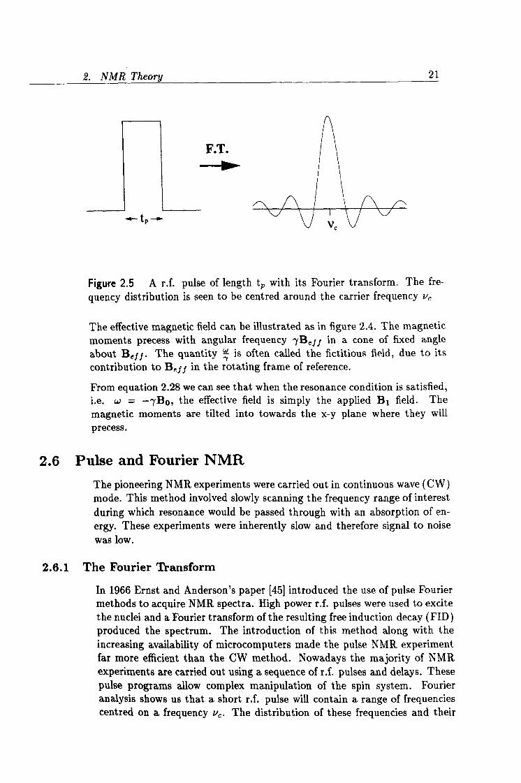
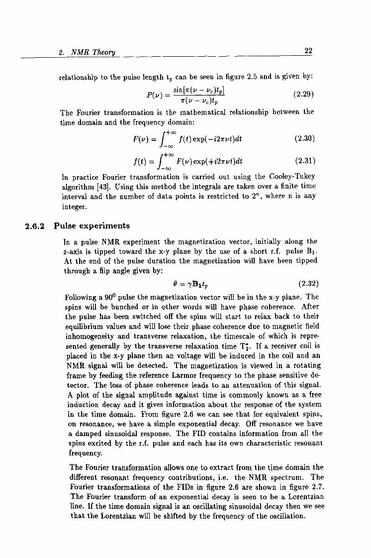
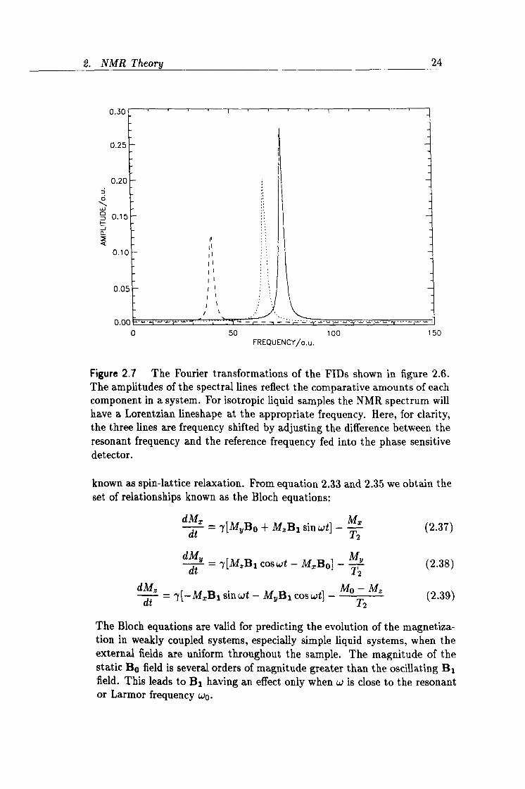
The Fourier transformation allows one to extract from the time domain the different resonant frequency contributions, i. e. the NMR spectrum. The Fourier transformations of the FIDs in figure 2.6 are shown in figure 2.7. The Fourier transform of an exponential decay is seen to be a Lorentzian line. If the time domain signal is an oscillating sinusoidal decay then we see that the Lorentzian will be shifted by the frequency of the oscillation.
2. NMR
2
7
O L W 00
H
J C- a
_1
23
1
r'; 1 F ;i 11 1"
I'. II ýIIý II il I 111. ýý"""ýý ý ý. ý;; ýq
l; lýll: lI I. Illvl`I111"ýi1ý
Iý1 11 f 'ij
I: ,ty 13
a J J. v^ IVI. V^ IV
TIME/microseconds 1.5x10⁵
Figure 2.6 The time response f(t) of a spin system subjected to three dis- tinct frequency shifts from the reference frequency. The signals are called free induction decays or FID's. For clarity the FID's have different ampli- tudes.
2.7 Relaxation and the Bloch Equations Felix Bloch [38] presented a series of equations which accounted for relaxation of the magnetization upon removal of the oscillating B1 field. He assumed that the magnetization decayed back to thermal equilibrium exponentially, but he assigned different characteristic time constants to the transverse and longitudinal relaxation. Assuming the static Bo field is oriented along the z axis the equations are:
dMX, y MX 'y (2.33)
dt T2 with solution:
Mx y(t) = M.,,, (0) exp(-t/T2) (2.34)
and:
with solution:
dMz (M. - Mo) (2.35) dt T1
[Mx(t) - Mo] = [M, (0) - Mo] exp(-t/T1) (2.36)
The decay of the transverse magnetization, with relaxation time T2, is com- monly known as transverse relaxation and the longitudinal relaxation T1, is
2. NMR
0.30
0.25
0.20
O
W
Z) 0.15 H J 0
o. 1 c
o. o:
o. o(
24
d iý ý ii iý iý iý
i iý
0 50 100 150 FREQUENCY/a. u.
Figure 2.7 The Fourier transformations of the FIDs shown in figure 2.6. The amplitudes of the spectral lines reflect the comparative amounts of each component in a system. For isotropic liquid samples the NMR spectrum will have a Lorentzian lineshape at the appropriate frequency. Here, for clarity, the three lines are frequency shifted by adjusting the difference between the resonant frequency and the reference frequency fed into the phase sensitive detector.
known as spin-lattice relaxation. From equation 2.33 and 2.35 we obtain the set of relationships known as the Bloch equations:
dM dt = y[MyBo + M, B1 sin wt] -
T2 (2.37)
dM ,y= 7[M, ýBl coswt - MBo] - Ty (2.38)
dz dsin
M0 Z,
Mz (2.39) 2
The Bloch equations are valid for predicting the evolution of the magnetiza- tion in weakly coupled systems, especially simple liquid systems, when the external fields are uniform throughout the sample. The magnitude of the static Bo field is several orders of magnitude greater than the oscillating B1 field. This leads to Bi having an effect only when w is close to the resonant or Larmor frequency wo.
2. NMR Theory 25
2.8 The Spectrometer
NMR spectrometers are used to detect and measure electromagnetic tran- sitions between energy levels created by applying a magnetic field to the sample. These transitions occur within the radio frequency range for typi- cally available strengths of the static magnetic field, and the corresponding resonance is detected using an r. f. transmitter-receiver coil.
The pulse NMR spectrometer generally carries out two distinct operations: (i) The transmitter has to provide short bursts of r. f. power to the sample under investigation. (ii) The receiver has to amplify and process the small NMR signals obtained.
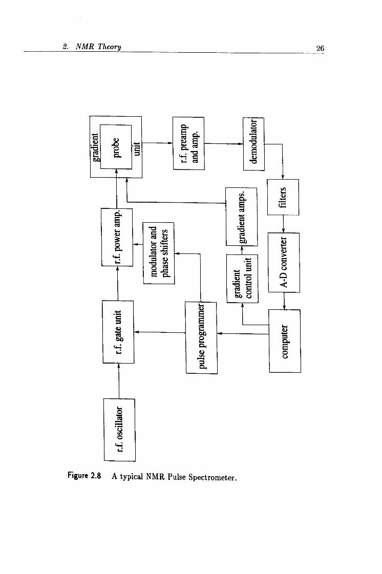
All the NMR experiments described in this thesis were performed using such a pulse NMR spectrometer, the general setup of which is fairly universal and is schematically illustrated in figure 2.8.
The r. f. oscillator is used in both the transmitter and receiver circuits. It functions at the Larmor frequency of the nuclei of interest which is related to the strength of the magnetic field.
In the transmitter circuit the r. f. gate unit switches the signal from the oscillator on and off under the direction of the pulse programmer. The output is then amplified to produce the r. f. pulses of sufficient power to excite the nuclear spin system.
In the receiver circuit the weak NMR signal is amplified by the pre-amplifier to a level suitable for demodulation. The demodulator's role is to convert the high frequency radio frequency into an audio frequency, leaving the NMR precession signal. The demodulated signal output is then passed through some audio filters which remove any noise from outside the sweep width. The digital signal is finally passed to the computer for data processing.
The more relevant components of the pulsed NMR spectrometer and their functions will be discussed in more detail in the following sections. A couple of excellent texts which describe the experimental considerations of using an NMR spectrometer are by Fukushima and Roeder [531 and by Martin, Martin and Delpuech [541.
2.8.1 The NMR Probe
The role of the NMR probe is twofold. Firstly it excites the nuclear spin system by transmitting r. f. power to the sample. Secondly it detects the small emfs generated by the bulk magnetization in the transverse plane. The most sensitive method of detection relies on the principle of induction, i. e. a changing magnetic field induces an electro motive force (emf) in a loop of electrical conductor through which the field passes [55]. The circuit is resonant at a frequency proportional to Fj'-C, The inductance of the coil is fixed and the capacitance is used to tune the LC circuit to the required
2. NMR Theo
a
cd Ö
I-ce
Cd
a)
04 O
Cl.
ý, O eý
..... ..., O
I-
O E "v
^b Cd
}' C C O
ö A
aý
a
O U
26
Figure 2.8 A typical NMR Pulse Spectrometer.
2. NMR Theory 27
frequency. At resonance the tuned circuit amplifies any voltage induced in the coil by a factor Q, referred to as the quality factor. To optimize the signal to noise ratio we desire a large value for Q. However there is a constraint placed on this. As Q is increased, so is the "ringdown" or the length of time the electronics of the probe take to recover. For some experiments, especially ones involving solids, it is desirable to sample the data as soon after the pulse as possible. Thus a small value of Q is required. The conflicting requirements
CT
R
L
Figure 2.9 An NMR sample probe circuit.
of the transmitter and receiver have provided an interesting challenge for probe designers over the years and many solutions have been proposed. A typical probe circuit is shown in figure 2.9. The matching capacitors cm are used match the impedance of the probe to that of the coaxial cable (5052).
2.8.2 The r. f. Transmitter
The purpose of the r. f. transmitter is to amplify the r. f. pulses to a level capable of exciting the nuclear spin system. The pulse power must quickly rise to its maximum value and return to zero in a short space of time, typical pulse lengths are of the order of a few microseconds. This allows the use of a single transmitter-receiver coil. As mentioned in section 2.6 the B1 field required to tip the magnetization through an angle of 0 is given by:
0= yB1tp (2.40)
The magnitude of the B1 field must be sufficient to excite the distribution of precessional frequencies of the spins. For liquid samples a typical B1 field is 10-4 T.
2. NMR
2.8.3 The r. f. Receiver
28
The receiver comprises several processing stages. The first unit, the pre- amplifier, is one of the most important. Any noise generated here will add to the signal and be amplified by the subsequent r. f. units. The demodulator
uses the r. f. oscillator to add to and subtract from the signal from the pre- amplifier. This produces a sum and a difference frequency signal. The high frequency signal is removed using a low pass filter leaving the demodulated NMR signal. The ADCs produce a digital signal which will undergo data
processing on a computer or workstation.
Chapter 3 NMR Relaxation Studies of PAN solutions
3.1 Introduction
The macroscopic consequences of nuclear magnetic relaxation have been dis- cussed in chapter 2 using the Bloch equations, but so far there has been no mention concerning the causes of this effect or the relationship with the molecular structure and dynamics. This chapter will outline the theory of the interaction of nuclear magnetic moments with their environment, and the theory will be applied to the experimental data acquired.
The foundations for the theory of nuclear spin relaxation were laid in the classic paper by Bloembergen, Purcell and Pound [1] and later modified by Kubo and Tomita [56]. Although this theory has been greatly devel- oped many of the ideas hold for a simple system where molecular motion is isotropic and random.
3.2 Mechanisms
3.2.1 General Principles
In an NMR experiment there are other magnetic fields present apart from the applied static Bo and oscillating B1 fields. It is these other randomly fluctuating fields which lead to relaxation back to thermal equilibrium. The most common and dominant of these local magnetic fields are the ones pro- duced by nuclear magnetic moments at the the sites of neighbouring spins. The thermally driven changes in the orientations of these neighbouring nu- clei lead to changes in the local magnetic field and if at the appropriate frequency can cause transitions between nuclear energy levels, i. e. relax- ation. The process can be thought of as the reverse of r. f. excitation with the time dependent spin interactions arising from thermally driven relative motions of the nuclei rather than from an oscillating r. f. field.
The theory of relaxation is most rigorously described using a quantum me- chanical approach. Here a more descriptive method will be used to give a picture of the physical interactions occurring.
We start by defining a time correlation function
G(T) = (bzo, (t) " bio, (t + r))eq (3.1)
The brackets < >eq represent an ensemble average taken over the macro- scopic system.
The time correlation function G(r) describes the similarities, on average, in blo, at a time 7- later. At short r it is expected that there is some
29
3. NMR Relaxation Studies of PAN solutions 30
1.0
0.8
5 0.6 C O
O N
0 0.4
o..
o. 1
f
f
-11 J [Alu 4xlu v-v
tau/seconds
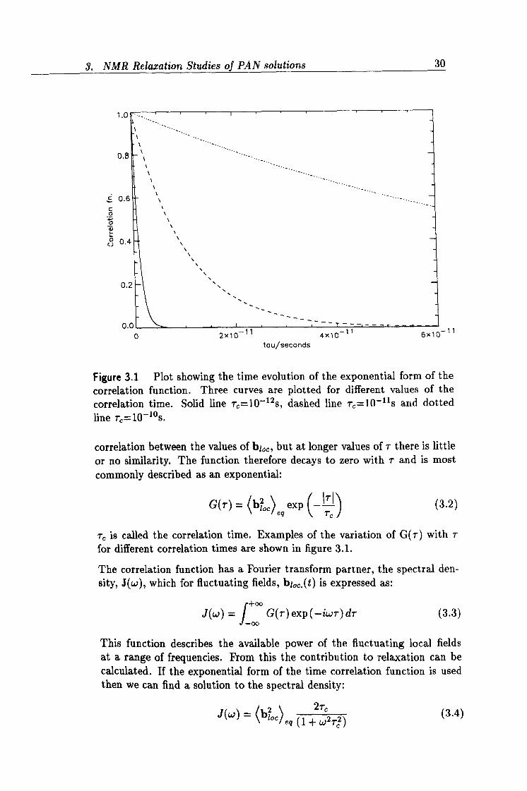
Figure 3.1 Plot showing the time evolution of the exponential form of the
correlation function. Three curves are plotted for different values of the correlation time. Solid line rC =10-12s, dashed line T, =10-lls and dotted line rß=10-10s.
correlation between the values of bi,,, but at longer values of 7- there is little
or no similarity. The function therefore decays to zero with r and is most commonly described as an exponential:
G(T) = (bloc)
exp (_ii. '\ 1
(3.2)
T, is called the correlation time. Examples of the variation of G(r) with 7- for different correlation times are shown in figure 3.1.
The correlation function has a Fourier transform partner, the spectral den- sity, J(w), which for fluctuating fields, bl,,. (t) is expressed as:
+00
J(w) =f G(r) exp (-iwr) dr (3.3)
This function describes the available power of the fluctuating local fields at a range of frequencies. From this the contribution to relaxation can be calculated. If the exponential form of the time correlation function is used then we can find a solution to the spectral density:
J(w) = (b0) 2r (3.4)
eq (1 + W2, r2)
3. NMR Relaxation Studies of PAN solutions 31
-6 'Cc=1x10 S
" tic=1x10⁻⁸ s Tc=1x10-'o s
z w J
a H U W a U,
In (FREQUENCY)
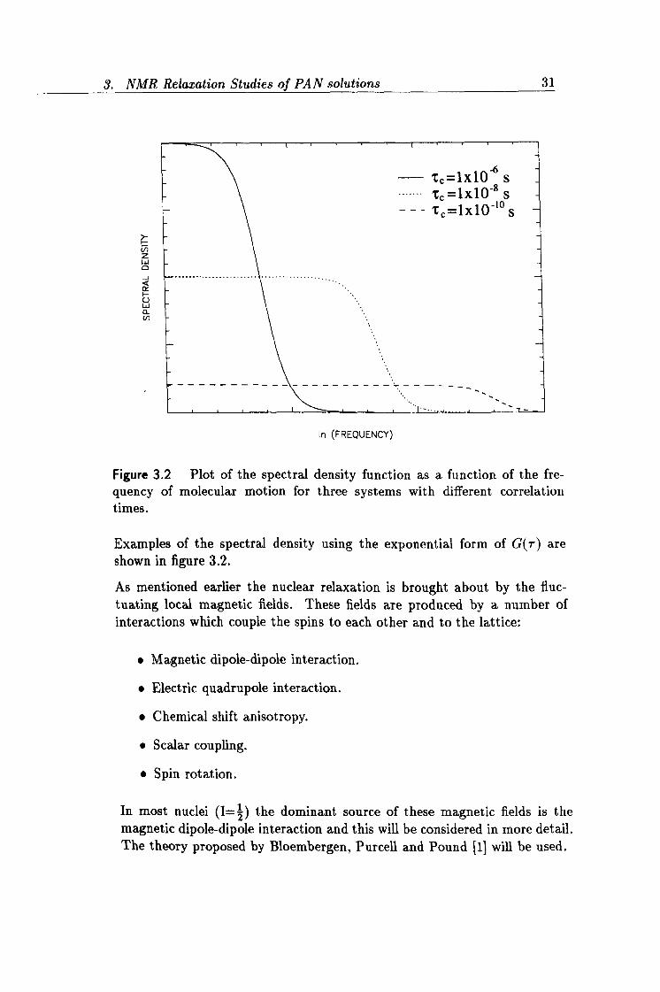
Figure 3.2 Plot of the spectral density function as a function of the fre-
quency of molecular motion for three systems with different correlation times.
Examples of the spectral density using the exponential form of G(r) are shown in figure 3.2.
As mentioned earlier the nuclear relaxation is brought about by the fluc- tuating local magnetic fields. These fields are produced by a number of interactions which couple the spins to each other and to the lattice:
" Magnetic dipole-dipole interaction.
" Electric quadrupole interaction.
" Chemical shift anisotropy.
" Scalar coupling.
" Spin rotation.
In most nuclei (1= 2) the dominant source of these magnetic fields is the magnetic dipole-dipole interaction and this will be considered in more detail. The theory proposed by Bloembergen, Purcell and Pound [11 will be used.
3. NMR Relaxation Studies of PAN solutions 32
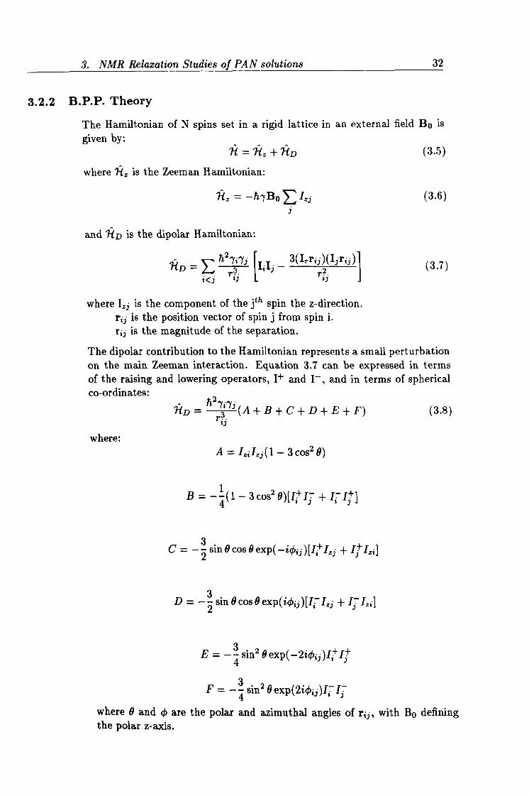
3.2.2 B. P. P. Theory
The Hamiltonian of N spins set in a rigid lattice in an external field Bo is given by:
R =lz+HD (3.5)
where 7 is the Zeeman Hamiltonian:
? (z - h7Bo > IZj (3.6)
and 'KD is the dipolar Hamiltonian:
h272'1ý 3(ITrtý)(Iýr=ý) RD (3.7)
< 13 tj rte r
where I3 is the component of the jth spin the z-direction. rte is the position vector of spin j from spin i. r; 3 is the magnitude of the separation.
The dipolar contribution to the Hamiltonian represents a small perturbation on the main Zeeman interaction. Equation 3.7 can be expressed in terms of the raising and lowering operators, I+ and I-, and in terms of spherical co-ordinates:
fD _ h2 3. (A-}-B+C+D+E+F) (3.8)
rt3
where: A IztIzj (1 -3 cost 9)
cost 8)[Ii I, + Ii I+
C=-3 sin 0 cos 0 exp(-iojj)[I; Izj + Ij IZi]
D= -3 sin0cos0exp(igij)[II Izj +Ij Izt]
E_-4 sine 0 exp(-2io- -)It Iý
F=-4 sin2 B exp(2igjj)I Iý-
where 0 and 0 are the polar and azimuthal angles of r13, with Bo defining the polar z-axis.
3. NMR Relaxation Studies of PAN solutions 33
N
I-
C
\ T2
In(Correlotion time)
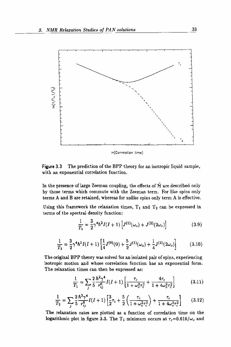
Figure 3.3 The prediction of the BPP theory for an isotropic liquid sample, with an exponential correlation function.
In the presence of large Zeeman coupling, the effects of ? -l are described only by those terms which commute with the Zeeman term. For like spins only terms A and B are retained, whereas for unlike spins only term A is effective.
Using this framework the relaxation times, T1 and T2 can be expressed in terms of the spectral density function:
Tl =
2y4h2I(I + 1) [J(1)(wo) + J(2)(2wo), (3.9)
1- =
314 h 21(1 + 1) [J(0)(o)
+ 2J(1)(wo) +1 j(2)(2wo)l (3.10)
The original BPP theory was solved for an isolated pair of spins, experiencing isotropic motion and whose correlation function has an exponential form. The relaxation times can then be expressed as:
1 274 (3.11)
i 13
T2 =52 g41(I +1)
[3 2 (1+rc2, r2
+ 1+T4wör2, (3.12)
sj 0
The relaxation rates are plotted as a function of correlation time on the logarithmic plot in figure 3.3. The Ti minimum occurs at r, =0.616/wo and
3. NMR Relaxation Studies of PAN solutions 34
180° 90°
'C-
y
ZZZl
Y r r r
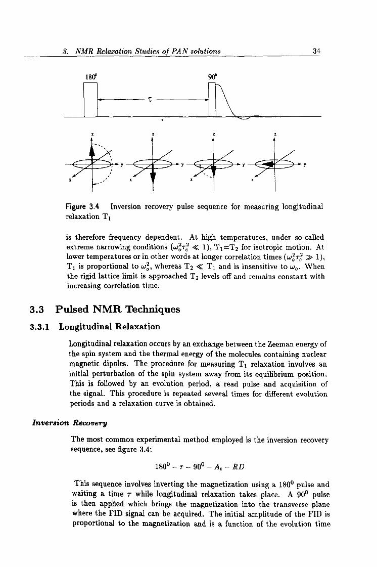
Figure 3.4 Inversion recovery pulse sequence for measuring longitudinal relaxation T1
is therefore frequency dependent. At high temperatures, under so-called extreme narrowing conditions (W2 -r, 2 « 1), T1=T2 for isotropic motion. At lower temperatures or in other words at longer correlation times (wö rý » 1), T1 is proportional to wö, whereas T2 « T1 and is insensitive to wo. When the rigid lattice limit is approached T2 levels off and remains constant with increasing correlation time.
3.3 Pulsed NMR Techniques
3.3.1 Longitudinal Relaxation
Longitudinal relaxation occurs by an exchange between the Zeeman energy of the spin system and the thermal energy of the molecules containing nuclear magnetic dipoles. The procedure for measuring T1 relaxation involves an initial perturbation of the spin system away from its equilibrium position. This is followed by an evolution period, a read pulse and acquisition of the signal. This procedure is repeated several times for different evolution periods and a relaxation curve is obtained.
Inversion Recovery
The most common experimental method employed is the inversion recovery sequence, see figure 3.4:
180°-r-90°-At-RD
This sequence involves inverting the magnetization using a 1800 pulse and waiting a time r while longitudinal relaxation takes place. A 90° pulse is then applied which brings the magnetization into the transverse plane where the FID signal can be acquired. The initial amplitude of the FID is proportional to the magnetization and is a function of the evolution time
3. NMR Relaxation Studies of PAN solutions 35
r. The experiment is repeated after waiting a recycle time, RD >_ 5T1, for different values of r. From the Bloch equations the form of the relaxation can be found:
dMz _
(Mz - Mo) (3.13) dt Ti
If M, = -Mo at t=0, then we have as a solution:
M, = Mo(1 - 2exp(-r/Ti)) (3.14)
As can be seen the relaxation in this case is exponential in nature. T1 can therefore be obtained either by aa straight line semi-logarithmic plot or by an exponential fit of the data. The method used to analyse the data in this thesis was the latter technique where a least squares approach was used to determine the values of Mo, T1 and k. k is a parameter which replaces the factor 2 in the above equation and is a measure of how accurately the pulse lengths have been set and also a measure of the distribution of flip angles arising from the inhomogeneities of the B1 field over the sample.
The major disadvantage of the inversion recovery method is the length of the recovery or recycle time. This is the time required for the magnetization to fully relax back to its equilibrium value. This has led to more novel pulse sequences being devised which incorporate rapid recycling. The fast inversion recovery method is one such technique [57].
3.3.2 Transverse Relaxation
In principle the transverse relaxation time T2 can be obtained, for isotropic liquids with a Lorentzian lineshape, by an exponential fit of the free induc- tion decay. However in practice, magnet inhomogeneity leads to a spatial spread of resonant frequencies throughout the sample. The decay of the FID therefore has two contributions. The first is from the natural random processes which bring the magnetization back to equilibrium. The second is from the inhomogeneity of the B° field. A revised relaxation time can be approximated as:
where
T+ 2B0 (3.15)
2 12-
ABO is the spread in magnetic field strength caused by the magnetic field inhomogeneities.
The linewidth at half height of a resonance line is generally expressed in terms of T2 and is a commonly used method for measuring this parameter:
Ov2 =1 (3.16) 7r2
Due to the reversible nature of the field imperfections it is possible, by using an appropriate pulse sequence, to overcome these effects. Special methods have been devised to cancel out this inhomogeneous broadening and these will be described here.
3. NMR Relaxation Studies of PAN solutions 36
Spin Echo Method
In 1950 Erwin Hahn [41] devised a method to circumvent the problems of field inhomogeneities in T2 measurements . He called this technique the spin echo method. The method consists of the following pulse sequence:
90°, -ýr-180°, -T-At-RD The effect of the sequence on the magnetization in the rotating frame is
shown schematically in figure 3.5.
The pulse sequence is repeated for several different values of T thus building
up a relaxation decay as a function of time. Once again the recycle time should be at least 5T1.
The spin echo method is limited in its use because of the effects of molecular diffusion. During the duration r it is possible that the spins will diffuse from
one part of the field to another. Due to the inhomogeneity of the magnet the resonance frequency of the spins will thus change in a random manner. The consequence of this will be a reduction in the amplitude of the spin echo acquired, given by [32]:
2T1 - 32
2 ^1 G2DT31 (3.17) Mt(2rr) Moexp ý(-T2 )3
where D is the self diffusion coefficient. G is the size of the background magnetic field gradients, assumed linear in spatial dependence, caused by the magnetic field inhomogeneity.
Carr Purcell Method
Carr and Purcell [461 introduced a method to diminish the effects of transla- tional diffusion, through inhomogeneous fields, on the measurement of trans- verse relaxation times. This technique, a modification of the Hahn spin-echo method involves applying a 900 pulse, followed by a train of 180° pulses.
900ß -T- [18O°,
-r- At - T-, n
1800 pulses are applied at times T, 27-, 4r, 6T, ....
These cause rephasing of the magnetization in the form of echoes at times r, 3rr, 5T, Tr, ....
The echoes alternate in phase due to the refocusing pulse flipping the magnetization between the +y' and -y' axes.
The Carr-Purcell sequence is considerably more efficient than the Hahn spin- echo experiment. A full train of echoes may be obtained in a single acqui- sition, whereas the corresponding experiment using the spin-echo method would require several acquisitions with a recycle time 5T1 between each one. Also by choosing a small value for rr, the effects of molecular diffusion can be reduced considerably, since for the Carr-Purcell sequence:
Mt(t) = Moexp [(t
T/ ]1
3y2G2Dr2t1
3. NMR Relaxation Studies of PAN solutions 37
Y
Y
Y
Y
Y
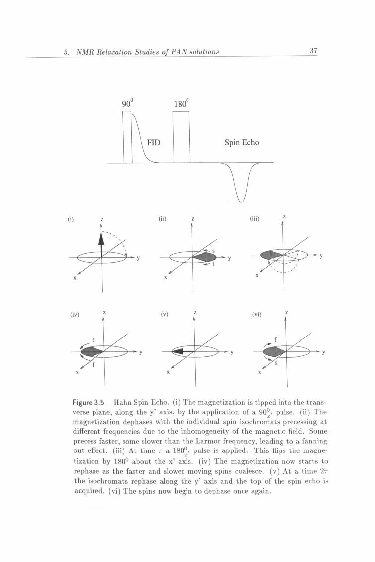
y
Figure 3.5 Hahn Spin Echo. (i) The magnetization is tipped into the trans- verse plane, along the y' axis, by the application of a 900, pulse. (ii) The magnetization dephases with the individual spin isochromats precessing at different frequencies due to the inhomogeneity of the magnetic field. Some precess faster, some slower than the Larmor frequency, leading to a fanning out effect. (iii) At time 7a 1800, pulse is applied. This flips the magne- tization by 1800 about the x' axis. (iv) The magnetization now starts to rephase as the faster and slower moving spins coalesce. (v) At a time 2r the isochromats rephase along the y' axis and the top of the spin echo is acquired. (vi) The spins now begin to dephase once again.
90 ° 180°
(iii) (i) z (ii) z
(iv) z (v) z (vi) Z
3. NMR Relaxation Studies of PAN solutions 38
where t=2nr for the nth echo. r values as short as a few hundred microseconds can be used, which thus reduces the value of the diffusion term.
Errors can still occur in the measurement of T2 using the Carr-Purcell method if the pulse lengths are not set accurately. Incomplete refocusing of the magnetization will occur which leads to an attenuation of the echo, and a smaller than expected T2 being obtained.
Meiboom Gill Method
Meiboom and Gill [58] modified the Carr-Purcell sequence in order to com- pensate for pulse length imperfections. This was achieved by simply altering the phase of the 180° pulse.
9U°, -T- 118001
-T- At - T-I 1 Jn
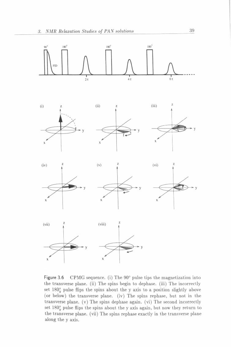
The 1800 pulses are applied along the y' axis, which is a 90° phase shift relative to the initial 90° pulse. All the echoes are refocussed along the positive y axis and therefore all have the equivalent phase. The consequences of the Meiboom-Gill modification in the rotating frame can be seen in figure 3.6. The 1800 pulse length has been inaccurately set to highlight the benefits of this method. After the first quasi 180° pulse the magnetization can be seen to have been displaced from the x-y plane. This leads to an attenuation of the echo amplitude upon rephasing. After a time r the second quasi 180° pulse is applied which leads to an exact return of the magnetization to the x-y plane. The second echo therefore has the correct amplitude as do all subsequent even numbered echoes. All the odd numbered echoes are attenuated slightly by an equal amount. The transverse relaxation time is therefore obtained by plotting the ampli- tude of the even numbered echoes against the echo time (4r, 8rr, 12rr...... ) and fitting the exponential decay.
3.4 Experimental Methodology
3.4.1 Sample Preparation
The polymer solution samples (dopes) used in the experiments described throughout this thesis were prepared using a polyacrylonitrile (PAN) sample (MW(wt. average) =65500). The solvent selected to dissolve the PAN was a 52%(by wt. ) NaSCNaq. solution. For comparison purposes the same strength of solvent was used to dissolve the solutions of varying PAN compositions. Although the system PAN/NASCNaq. has high commercial value, the study of its solution properties have not been widely published [25,24]. A study by Geller and Eftina [22] of the concentration dependence of the viscosity
3. NMR Relaxation Studies of PAN solutions 39
900 180° 180° 180
6t
(viii Z
Y
Y
Y
Y
Y
Y
y
y
Figure 3.6 CPMG sequence. (i) The 900 pulse tips the magnetization into the transverse plane. (ii) The spins begin to dephase. (iii) The incorrectly set 180'. pulse flips the spins about the y axis to a position slightly above (or below) the transverse plane. (iv) The spins rephase, but not in the transverse plane. (v) The spins dephase again. (vi) The second incorrectly set 180, pulse flips the spins about the y axis again, but now they return to the transverse plane. (vii) The spins rephase exactly in the transverse plane along the y axis.
/viiil
2t 4t
(ii) z (iii) (i) z
(iv) (v) Z (vil Z
3. NMR Relaxation Studies of PAN solutions 40
showed a minimum at 50-55% (by wt. ) NaSCN and therefore a concentration in this range was chosen.
To prepare the PAN dopes the NaSCN solution was heated to a tempera- ture of 60-70°C, and the PAN was added gradually with continuous stirring. The stirring was continued for approximately 20 minutes or until the solu- tion appeared homogeneous. The sample was then placed in a oven at a temperature of 50°C for 2-3 days to allow any air bubbles to rise.
The solutions were transferred to the 10mm diameter NMR tubes using a specially adapted syringe. This allowed the dopes to be placed in the bottom of the tube without leaving residue on the sides of the tube, which could lead to spurious NMR signals.
A series of dopes were able to be prepared, up to a maximum composition of 15% (by wt. ) PAN. Above this composition the dopes become too viscous and it is impossible to prepare homogeneous solutions.
3.4.2 Instrumentation
The NMR relaxation experiments were carried out using a Bruker CXP-100 NMR spectrometer, the details of which are given in the next section. Also described is the Resonance Instruments MARAN-20 bench-top spectrometer which was used to carry out the majority of the experiments described in the subsequent chapters.
Bruker CXP-100
The CXP-100 NMR spectrometer was used with a proton resonance fre- quency of 60MHz. The magnet is a water cooled electromagnet with a 19F field frequency lock which aids stabilization of the magnetic field. The high power amplifier produces a 900 pulse length of 1.5 us in a 12mm diameter coil, and the instrumentation has a dead time of 8 ps. The dead time, which is the time taken for the probe electronics to recover after the r. f. pulse, incorporates the probe ring-down time and the filter settle time before ac- quisition can commence.
The Bruker CXP spectrometer uses the Redfield method for data acquisition. This technique employs one ADC for alternating acquisition of real and imaginary data points. The dwell time has a minimum value of 4µs which means that the temporal spacing between each acquired point in the real or imaginary plane is at least 8 µs. Upon Fourier transformation we find that the sweepwidth (SW) is given by:
ý SW =1 2* DWELL 3.19
The maximum sweepwidth is therefore 125 kHz.
The CXP-100 has variable temperature capabilities. The temperature changes are achieved by passing a stream of gas over an electrically heated wire coil.
3. NMR Relaxation Studies of PAN solutions 41
The gas temperature is monitored before passing over the sample by use of a thermocouple which is connected to the temperature controller. The work- ing range of the unit is 240K to 360K and the time taken for temperature
stabilization is approximately 20 minutes.
The computing capabilities are quite limited on the CXP and so the post acquisition data processing is carried out elsewhere. The data is first con- verted from the Bruker data format to ascii format using a Hewlett-Packard machine. It is then transferred to one of a number of Sun Sparcstations which have a number of data manipulation programs running under a Unix operating system, see section 3.4.3.
Resonance Instruments MARAN-20
The Resonance Instruments MARAN-20 is a benchtop NMR spectrometer with a permanent magnet. The operating frequency for protons is 20.2 MHz and a second probe for "Na has an operating frequency of 5.3 MHz. The machine has a lower power amplifier (300 W) than the CXP-100 and this is reflected by the longer 90° pulse length of 2.2 µs. The r. f. coils allow a sample tube diameter of 10mm and the field is homogeneous over a sample length of 14mm.
The MARAN-20 employs the quadrature method of detection. Using two ADC's the real and imaginary data is captured simultaneously. The mini- mum dwell time is 0.5 ps which leads to a sweepwidth of 2MHz.
The proton probe has a set of gradient coils which produce a gradient per- pendicular to the Bo field and parallel with the cylindrical sample tube axis. The maximum gradient strength possible is 203 Gcm-1 and this allows the study of the slow translational self-diffusion of polymers in solution. Variable temperature studies are also possible on the MARAN-20 using a similar protocol and range to that on the CXP-100.
3.4.3 Data Fitting Programs
Relaxation data acquired during an NMR experiment generally is not too useful before analysis. Both transverse and longitudinal relaxation data need to be fitted using exponential functions. Often these relaxation curves may appear to be single exponential in nature, but upon further analysis they are found to be multi-exponential and require more complicated fitting pro- cedures to extract useful information. The parameters obtained are usually assigned physical significance in terms of their location and mobility in the system. This is the case in a wide variety of fields, one such example is the interpretation of Ti and T2 relaxation times for water protons in complex aqueous systems such as living tissue [59,60,61].
Relaxation curves can be analysed using a variety of mathematical methods. These range from simple logarithmic plotting [621 to difference minimization
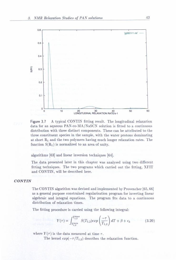
3. NMR Relaxation Studies of PAN solutions 42
0.6 'jgO601 r1. rat'
0.5
0.4
0.3 cn
0.2
0.1
0 10 20 30 40 50 60 LONGITUDINAL RELAXATION RATE/s-1
Figure 3.7 A typical CONTIN fitting result. The longitudinal relaxation data for an aqueous PAN-co-MA/NaSCN solution is fitted to a continuous distribution with three distinct components. These can be attributed to the three constituent species in the sample, with the water protons dominating at short Rl and the two polymers having much longer relaxation rates. The function S(R1) is normalized to an area of unity.
algorithms [63] and linear inversion techniques [64].
The data presented later in this chapter was analysed using two different fitting techniques. The two programs which carried out the fitting, XFIT and CONTIN, will be described here.
CONTIN
The CONTIN algorithm was devised and implemented by Provencher [65,66] as a general purpose constrained regularisation program for inverting linear algebraic and integral equations. The program fits data to a continuous distribution of relaxation times.
The fitting procedure is carried using the following integral:
JTmax Y(r) _
T"'
S(Ti, 2)exp dT +ß+ Ek (3.20) T ,n T1,2
where Y(r) is the data measured at time r. The kernel exp(-7-/T1,2) describes the relaxation function.
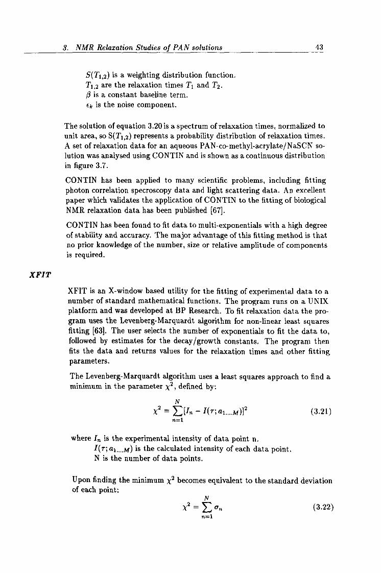
3. NMR Relaxation Studies of PAN solutions 43
S(T1,2) is a weighting distribution function. T1,2 are the relaxation times Tl and T2. 0 is a constant baseline term. ck is the noise component.
The solution of equation 3.20 is a spectrum of relaxation times, normalized to unit area, so S(T1,2) represents a probability distribution of relaxation times. A set of relaxation data for an aqueous PAN-co-methyl-acrylate/NaSCN so- lution was analysed using CONTIN and is shown as a continuous distribution in figure 3.7.
CONTIN has been applied to many scientific problems, including fitting photon correlation specroscopy data and light scattering data. An excellent paper which validates the application of CONTIN to the fitting of biological NMR relaxation data has been published [67].
CONTIN has been found to fit data to multi-exponentials with a high degree of stability and accuracy. The major advantage of this fitting method is that no prior knowledge of the number, size or relative amplitude of components is required.
XFIT
XFIT is an X-window based utility for the fitting of experimental data to a number of standard mathematical functions. The program runs on a UNIX platform and was developed at BP Research. To fit relaxation data the pro- gram uses the Levenberg-Marquardt algorithm for non-linear least squares fitting [63]. The user selects the number of exponentials to fit the data to, followed by estimates for the decay/growth constants. The program then fits the data and returns values for the relaxation times and other fitting parameters.
The Levenberg-Marquardt algorithm uses a least squares approach to find a minimum in the parameter X2, defined by:
N
X2 = E[In. - I(r; a,.... M)]2 (3.21)
n=1
where It, is the experimental intensity of data point n. I(r; a,.... M) is the calculated intensity of each data point. N is the number of data points.
Upon finding the minimum X2 becomes equivalent to the standard deviation of each point:
N
X2 _Eo, (3.22) nsl
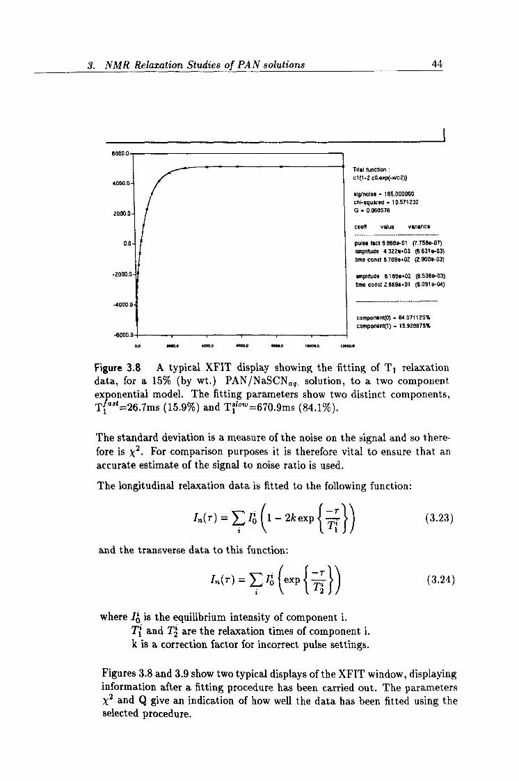
3. NMR Relaxation Studies of PAN solutions 44
Trial function : c1(1-2. c0. ep(-xlc2))
sig/nolse - 165.000000
chi-squared - 10.571232 0 -0.060576
coeft value Variance
pulse fact 9.868e-01 (7.758e-07)
amplitude 4.322e. 03 (6.631e-03) time const 6.709e. 02 (2.900e-03)
amplitude 8.1698+02 (5.536e-03) time tonst 2.669e+01 (5.0918-04)
component(O) - 84.071125%
component(1) - 15.928875%
Figure 3.8 A typical XFIT display showing the fitting of T1 relaxation data, for a 15% (by wt. ) PAN/NaSCNaq. solution, to a two component exponential model. The fitting parameters show two distinct components, Tlf°°t=26.7ms (15.9%) and T1-b°w=670.9ms (84.1%).
The standard deviation is a measure of the noise on the signal and so there- fore is X2. For comparison purposes it is therefore vital to ensure that an accurate estimate of the signal to noise ratio is used.
The longitudinal relaxation data is fitted to the following function:
- 1)
In(r) _ Iö 1- 2kexp TT (3.23) 1
and the transverse data to this function:
In(r) _ Iö exp ý (3.24)
where Io is the equilibrium intensity of component i. Tl and T2 are the relaxation times of component i. k is a correction factor for incorrect pulse settings.
Figures 3.8 and 3.9 show two typical displays of the XFIT window, displaying information after a fitting procedure has been carried out. The parameters x2 and Q give an indication of how well the data has been fitted using the selected procedure.
0.0 2000A 4000.0 4000.0 00000 10000.0 100000
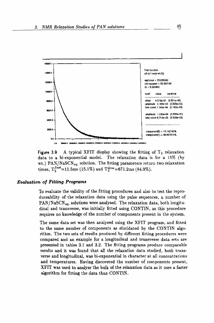
3. NMR Relaxation Studies of PAN solutions 45
18000.0
4{006.0
12000.0
t0000A
00001
60001
4000.
2000.
0
Trial function:
cO. (ct. exp(-, c2))
Sig/noise - 25.000000
chi-squared - 85.503188 Q-0.000000
C08N value variance
offset 4.515e+01 (9.051e+00)
amplitude 2.189e. 03 (2.1525e+02) time tonst 1.145e+04 (2.162e+03)
amplitude 1.230e+04 (3.9968+01) time const 6.7120+05 (3.6368+03)
component(0) " 15.1021 B5%
component(1) . 84.897815%
Figure 3.9 A typical XFIT display showing the fitting of T2 relaxation data to a bi-exponential model. The relaxation data is for a 15% (by
wt. ) PAN/NaSCNaq. solution. The fitting parameters return two relaxation times, Tfa, st=11.5ms (15.1%) and T2ý°w=671.2ms (84.9%).
Evaluation of Fitting Programs
To evaluate the validity of the fitting procedures and also to test the repro- duceability of the relaxation data using the pulse sequences, a number of PAN/NaSCNaq, solutions were analysed. The relaxation data, both longitu- dinal and transverse, was initially fitted using CONTIN, as this procedure requires no knowledge of the number of components present in the system.
The same data set was then analysed using the XFIT program, and fitted to the same number of components as elucidated by the CONTIN algo- rithm. The two sets of results produced by different fitting procedures were compared and an example for a longitudinal and transverse data sets are presented in tables 3.1 and 3.2. The fitting programs produce comparable results and it was found that all the relaxation data studied, both trans- verse and longitudinal, was bi-exponential in character at all concentrations and temperatures. Having discovered the number of components present, XFIT was used to analyse the bulk of the relaxation data as it uses a faster algorithm for fitting the data than CONTIN.
0.0 s0eo 10000W. 0 +000000.0 70000000 2900000.0 00000000 0000000.0 4000000.0 4100000.0 00000000
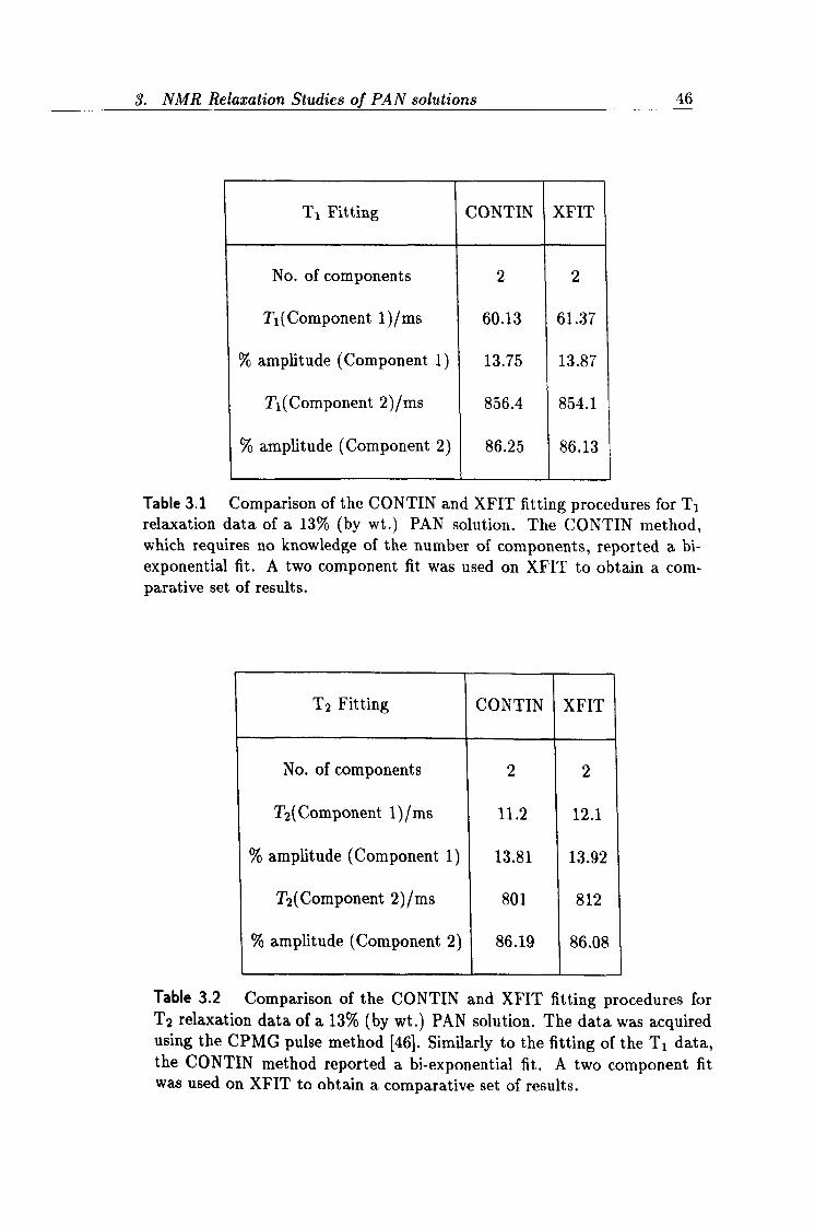
3. NMR Relaxation Studies of PAN solutions 46
Tl Fitting CONTIN XFIT
No. of components 2 2
T1(Component 1)/ms 60.13 61.37
% amplitude (Component 1) 13.75 13.87
T1(Component 2)/ms 856.4 854.1
% amplitude (Component 2) 86.25 86.13
Table 3.1 Comparison of the CONTIN and XFIT fitting procedures for T1 relaxation data of a 13% (by wt. ) PAN solution. The CONTIN method, which requires no knowledge of the number of components, reported a bi- exponential fit. A two component fit was used on XFIT to obtain a com- parative set of results.
T2 Fitting CONTIN XFIT
No. of components 2 2
T2(Component 1)/ms 11.2 12.1
% amplitude (Component 1) 13.81 13.92
T2(Component 2)/ms 801 812
% amplitude (Component 2) 86.19 86.08
Table 3.2 Comparison of the CONTIN and XFIT fitting procedures for T2 relaxation data of a 13% (by wt. ) PAN solution. The data was acquired using the CPMG pulse method [46]. Similarly to the fitting of the T1 data, the CONTIN method reported a bi-exponential fit. A two component fit was used on XFIT to obtain a comparative set of results.
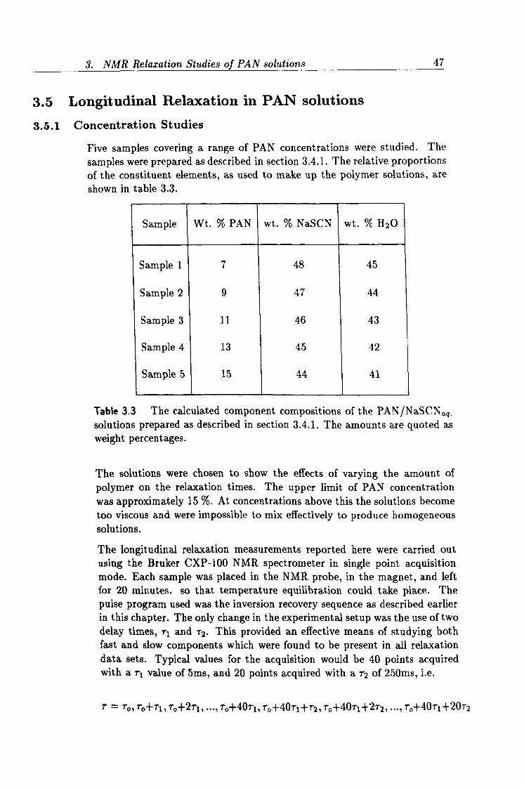
3. NMR Relaxation Studies of PAN solutions 47
3.5 Longitudinal Relaxation in PAN solutions
3.5.1 Concentration Studies
Five samples covering a range of PAN concentrations were studied. The
samples were prepared as described in section 3.4.1. The relative proportions of the constituent elements, as used to make up the polymer solutions, are shown in table 3.3.
Sample Wt. % PAN wt. % NaSCN wt. % H2O
Sample 17 48 45
Sample 29 47 44
Sample 3 11 46 43
Sample 4 13 45 42
Sample 5 15 44 41
Table 3.3 The calculated component compositions of the PAN/NaSCNa, q. solutions prepared as described in section 3.4.1. The amounts are quoted as weight percentages.
The solutions were chosen to show the effects of varying the amount of polymer on the relaxation times. The upper limit of PAN concentration was approximately 15 %. At concentrations above this the solutions become too viscous and were impossible to mix effectively to produce homogeneous solutions.
The longitudinal relaxation measurements reported here were carried out using the Bruker CXP-100 NMR spectrometer in single point acquisition mode. Each sample was placed in the NMR probe, in the magnet, and left for 20 minutes. so that temperature equilibration could take place. The pulse program used was the inversion recovery sequence as described earlier in this chapter. The only change in the experimental setup was the use of two delay times, -rl and r2. This provided an effective means of studying both fast and slow components which were found to be present in all relaxation data sets. Typical values for the acquisition would be 40 points acquired with arl value of 5ms, and 20 points acquired with a r2 of 250ms, i. e.
T= To, To+T1, To+2T1, ..., To+40T1, To+40T1+T2, To+40T1+2T2, ..., Tp+40T1+20T2
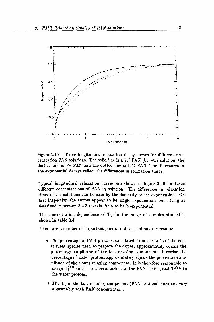
3. NMR Relaxation Studies of PAN solutions 48
1.5
1.0
ö 0.5 ö N 4)
C 01 0
0.0
-0.5
-1.0
i ý. /
i . - i i
i i . -
." //
/ .'
01234 TIME/seconds
Figure 3.10 Three longitudinal relaxation decay curves for different con- centration PAN solutions. The solid line is a 7% PAN (by wt. ) solution, the dashed line is 9% PAN and the dotted line is 11% PAN. The differences in the exponential decays reflect the differences in relaxation times.
Typical longitudinal relaxation curves are shown in figure 3.10 for three different concentrations of PAN in solution. The differences in relaxation times of the solutions can be seen by the disparity of the exponentials. On first inspection the curves appear to be single exponentials but fitting as described in section 3.4.3 reveals them to be bi-exponential.
The concentration dependence of T1 for the range of samples studied is shown in table 3.4.
There are a number of important points to discuss about the results:
" The percentage of PAN protons, calculated from the ratio of the con- stituent species used to prepare the dopes, approximately equals the percentage amplitude of the fast relaxing component. Likewise the percentage of water protons approximately equals the percentage am- plitude of the slower relaxing component. It is therefore reasonable to assign Tia't to the protons attached to the PAN chains, and Tit°w to the water protons.
" The Tl of the fast relaxing component (PAN protons) does not vary appreciably with PAN concentration.
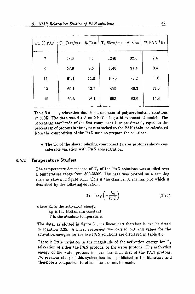
3. NMR Relaxation Studies of PAN solutions 49
wt. % PAN Ti Fast/ms % Fast T1 Slow/ms % Slow % PAN 'Hs
7 58.0 7.5 1240 92.5 7.4
9 57.9 9.6 1140 91.4 9.4
11 61.4 11.8 1080 88.2 11.6
13 60.1 13.7 853 86.3 13.6
15 60.5 16.1 693 83.9 15.8
Table 3.4 T1 relaxation data for a selection of polyacrylonitrile solutions at 300K. The data was fitted on XFIT using a bi-exponential model. The
percentage amplitude of the fast component is approximately equal to the percentage of protons in the system attached to the PAN chain, as calculated from the composition of the PAN used to prepare the solutions.
" The T1 of the slower relaxing component (water protons) shows con- siderable variation with PAN concentration.
3.5.2 Temperature Studies
The temperature dependence of T1 of the PAN solutions was studied over a temperature range from 300-360K. The data was plotted on a semi-log scale as shown in figure 3.11. This is the classical Arrhenius plot which is described by the following equation:
Tl = exp - E,, ) (3.25)
kBT
where Eq, is the activation energy. kB is the Boltzmann constant. T is the absolute temperature.
The data, as plotted in figure 3.11 is linear and therefore it can be fitted to equation 3.25. A linear regression was carried out and values for the activation energies for the five PAN solutions are displayed in table 3.5.
There is little variation in the magnitude of the activation energy for T1 relaxation of either the PAN protons, or the water protons. The activation energy of the water protons is much less than that of the PAN protons. No previous study of this system has been published in the literature and therefore a comparison to other data can not be made.
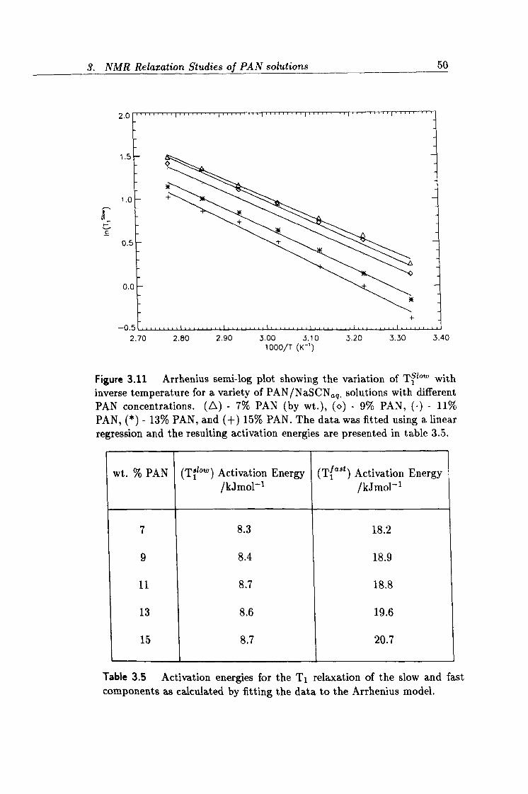
3. NMR Relaxation Studies of PAN solutions
2.0
1.5
1.0
I- c
0.5
0.0
-0.5 2.70 2.80 2.90 3.00 3.10
1000/T (K-')
50
3.20 3.30 3.40
Figure 3.11 Arrhenius semi-log plot showing the variation of Ti 10 L with inverse temperature for a variety of PAN/NaSCN,, 9. solutions with different PAN concentrations. (A) - 7% PAN (by wt. ), (o) - 9% PAN, (") - 11% PAN, (*) - 13% PAN, and (+) 15% PAN. The data was fitted using a linear regression and the resulting activation energies are presented in table 3.5.
wt. % PAN (T1l0W) Activation Energy (Tiast) Activation Energy /kJmol-1 /kJmol-1
7 8.3 18.2
9 8.4 18.9
11 8.7 18.8
13 8.6 19.6
15 8.7 20.7
Table 3.5 Activation energies for the Tl relaxation of the slow and fast components as calculated by fitting the data to the Arrhenius model.
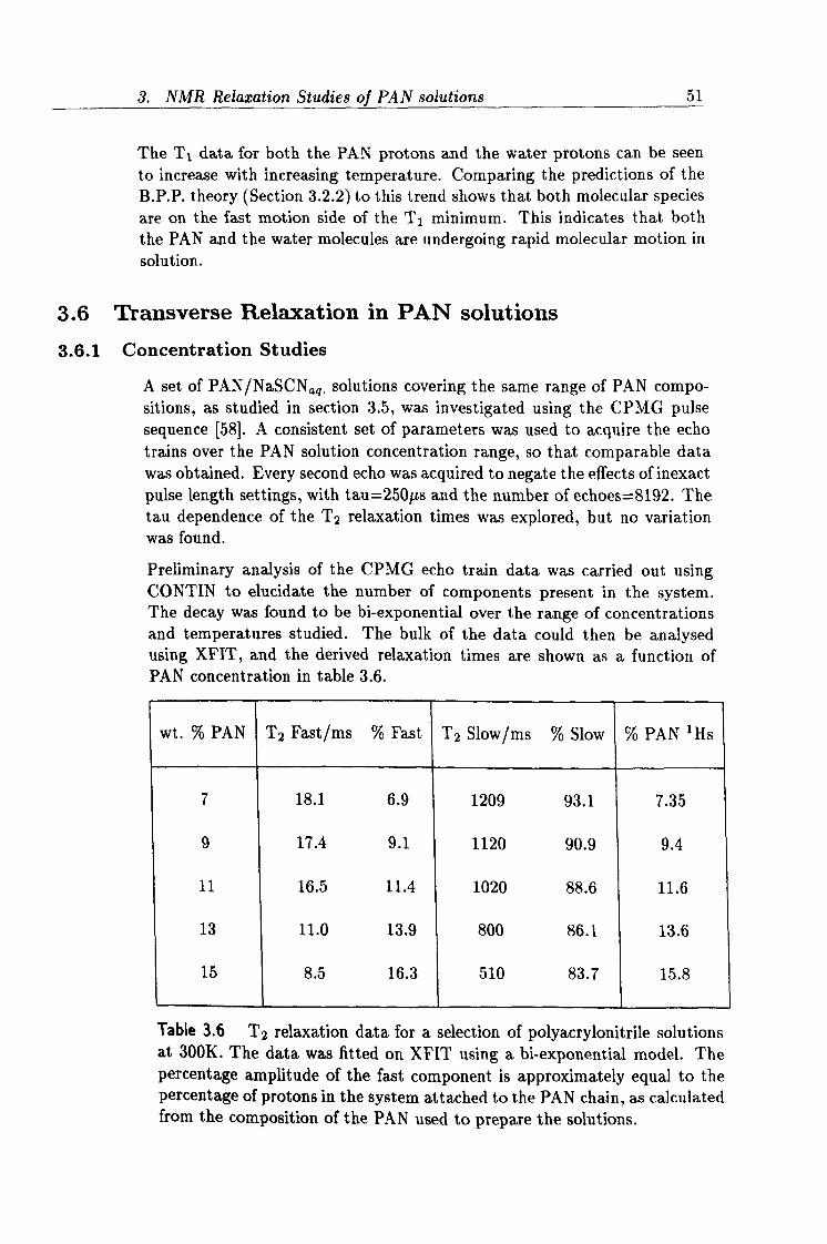
3. NMR Relaxation Studies of PAN solutions 51
The Tl data for both the PAN protons and the water protons can be seen to increase with increasing temperature. Comparing the predictions of the B. P. P. theory (Section 3.2.2) to this trend shows that both molecular species are on the fast motion side of the T1 minimum. This indicates that both the PAN and the water molecules are undergoing rapid molecular motion in solution.
3.6 Transverse Relaxation in PAN solutions 3.6.1 Concentration Studies
A set of PAN/Na5CNQq. solutions covering the same range of PAN compo- sitions, as studied in section 3.5, was investigated using the CPMG pulse sequence [58]. A consistent set of parameters was used to acquire the echo trains over the PAN solution concentration range, so that comparable data was obtained. Every second echo was acquired to negate the effects of inexact pulse length settings, with tau=250µs and the number of echoes=8192. The tau dependence of the T2 relaxation times was explored, but no variation was found.
Preliminary analysis of the CPMG echo train data was carried out using CONTIN to elucidate the number of components present in the system. The decay was found to be bi-exponential over the range of concentrations and temperatures studied. The bulk of the data could then be analysed using XFIT, and the derived relaxation times are shown as a function of PAN concentration in table 3.6.
wt. % PAN T2 Fast/ms % Fast T2 Slow/ms % Slow % PAN 'Hs
7 18.1 6.9 1209 93.1 7.35
9 17.4 9.1 1120 90.9 9.4
11 16.5 11.4 1020 88.6 11.6
13 11.0 13.9 800 86.1 13.6
15 8.5 16.3 510 83.7 15.8
Table 3.6 T2 relaxation data for a selection of polyacrylonitrile solutions at 300K. The data was fitted on XFIT using a bi-exponential model. The percentage amplitude of the fast component is approximately equal to the percentage of protons in the system attached to the PAN chain, as calculated from the composition of the PAN used to prepare the solutions.
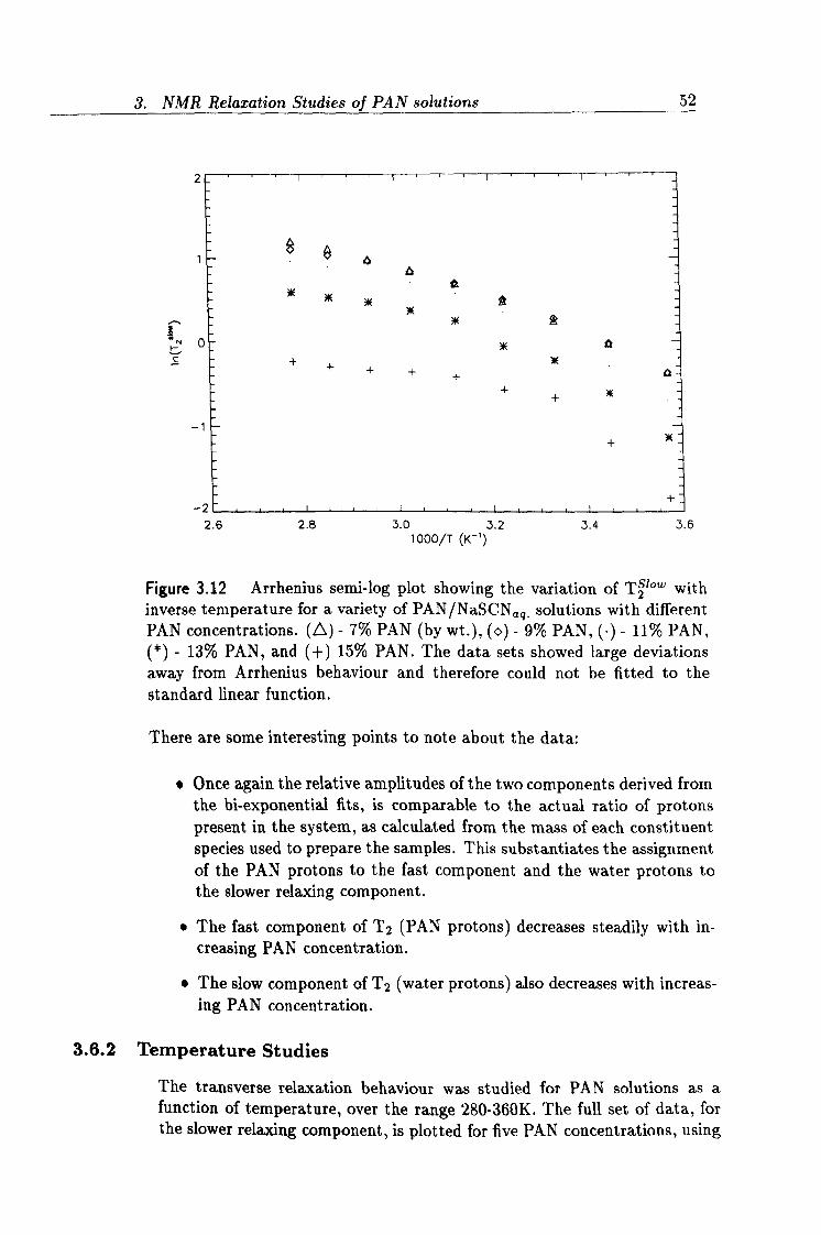
3. NMR Relaxation Studies of PAN solutions 52
2
..
C
- 1,
2.6 2.8 3.0 3.2 3.4 3.6 1 000/T (K-')
g 8 Q a
lot
Figure 3.12 Arrhenius semi-log plot showing the variation of T2 OW with inverse temperature for a variety of PAN/NaSCN,,, q. solutions with different PAN concentrations. (A) - 7% PAN (by wt. ), (o) - 9% PAN, (") - 11% PAN, (*) - 13% PAN, and (+) 15% PAN. The data sets showed large deviations away from Arrhenius behaviour and therefore could not be fitted to the standard linear function.
There are some interesting points to note about the data:
" Once again the relative amplitudes of the two components derived from the bi-exponential fits, is comparable to the actual ratio of protons present in the system, as calculated from the mass of each constituent species used to prepare the samples. This substantiates the assignment of the PAN protons to the fast component and the water protons to the slower relaxing component.
" The fast component of T2 (PAN protons) decreases steadily with in- creasing PAN concentration.
" The slow component of T2 (water protons) also decreases with increas- ing PAN concentration.
3.6.2 Temperature Studies
The transverse relaxation behaviour was studied for PAN solutions as a function of temperature, over the range 280-360K. The full set of data, for the slower relaxing component, is plotted for five PAN concentrations, using
3. NMR Relaxation Studies of PAN solutions 53
an Arrhenius semi-logarithmic scale, in figure 3.12. The temperature shows deviation away from the linear plot predicted by the Arrhenius expression. The molecular dynamics determining the transverse relaxation are thought to be too complicated to be described fully using a simple Arrhenius analysis, and therefore activation energies could not be derived.
As found for the Ti data, both the T2 components increase in value with increasing temperature. This confirms that the system is in the fast motion regime. As the temperature increases T1 --> T2 for the water protons. For the PAN component T1 > T2 which suggests that the protons on the PAN chain are undergoing some sort of anisotropic motion.
Chapter 4 Self Diffusion Measurements
4.1 Introduction The translational molecular diffusion of polymer chains and solvent molecules in polymer solutions has been extensively studied ever since measurements in these systems were able to be carried out. The diffusion is influenced by the polymer concentration, the sample temperature, the size and shape of the polymer and solvent and the interactions between them. The self diffusion coefficient of the constituent species gives a measure of their translational mobility and can be shown to be related to the intrinsic molecular proper- ties of both the polymer and the solvent. This subject has been covered in a number of review articles [68,69,70]
The diffusion of molecules can be studied using a number of experimen- tal techniques. These include light scattering, radioactive tracing, forced Raleigh scattering and nuclear magnetic resonance. The pulsed field gradi- ent NMR (PFGNMR) method has many advantages over the other available techniques:
" It allows the diffusion within a system to be probed non-invasively.
" It can provide information about restrictions within the system. In heterogeneous materials, parameters such as the dimensions of the boundaries can be measured.
" It measures the diffusion coefficient of the species directly. Some of the other methods indirectly determine this quantity by relating it to macroscopic measurements.
" The method is not limited to single phase liquid state samples. It al- lows the study of molecules confined within heterogeneous solid porous structures.
" It produces very accurate and reproducible results (1-2% errors).
The only disadvantage of the PFGNMR technique is imposed upon it by the maximum strength of the magnetic field gradients. This leads to a limitation being placed on the diffusion coefficient of around 10-9-10-1°cm2s-1. This area has also been comprehensively reviewed [71,72,73]
54
. j. Self Diffusion Measurements 55
4.2 Self Diffusion 4.2.1 General
Diffusion is the process by which matter is transported from one part of a system to another, and is a consequence of Brownian motion. The movement is chaotic and random and is often modelled by a random walk process with a characteristic diffusion coefficient. The definition and measurement of the diffusion coefficient is based upon Fick's laws of diffusion. For self diffusion of a particle in an unrestricted system, this is defined by Fick's Second Law of Diffusion:
Oc(r, t) _
ä2c(r, t) ö2c(r, t) 82c(r, t) (4.1)
at -D axe + &y2 +a Z2
where D is the self diffusion coefficient. c(r, t) is the concentration at a particular spatial and temporal posi-
tion.
In the study of diffusion using NMR it is often convenient to introduce the probability density function, P(r, OIro). This function also obeys the diffusion equation:
äP(r, OI ro) _D
a2P(r, Af ro) + a2P(r, Air. )
+ a2P(r, A r0) (4.2) OA äx2 äy2 0z2
where P(r, A Iro) is the probability of finding a particle at a position r, at a time A, given that it was originally at a position r0.
Solutions to the diffusion equation may be obtained for a wide variety of initial and boundary conditions [74]. The solution of equation 4.2 by con- ventional methods for unrestricted diffusion with an initial distribution of a delta function, P(r, A= 01r0) = 5(r0 - r), leads to a Gaussian distribution with respect to the displacement:
P(r, Air. ) = (4rD0)-3/2 exp (r - ro)2 (4.3)
4DA
The calculation of the mean square displacement is given by the Einstein- Smoluchowski equation:
< (r(0) - r0)2 >= 6DA (4.4)
Likewise in one dimension we have the following equation for the distribution:
P(x, ýýxo) . (4rD0)-1/2 exp - (X
4D A )Z
(4.5)
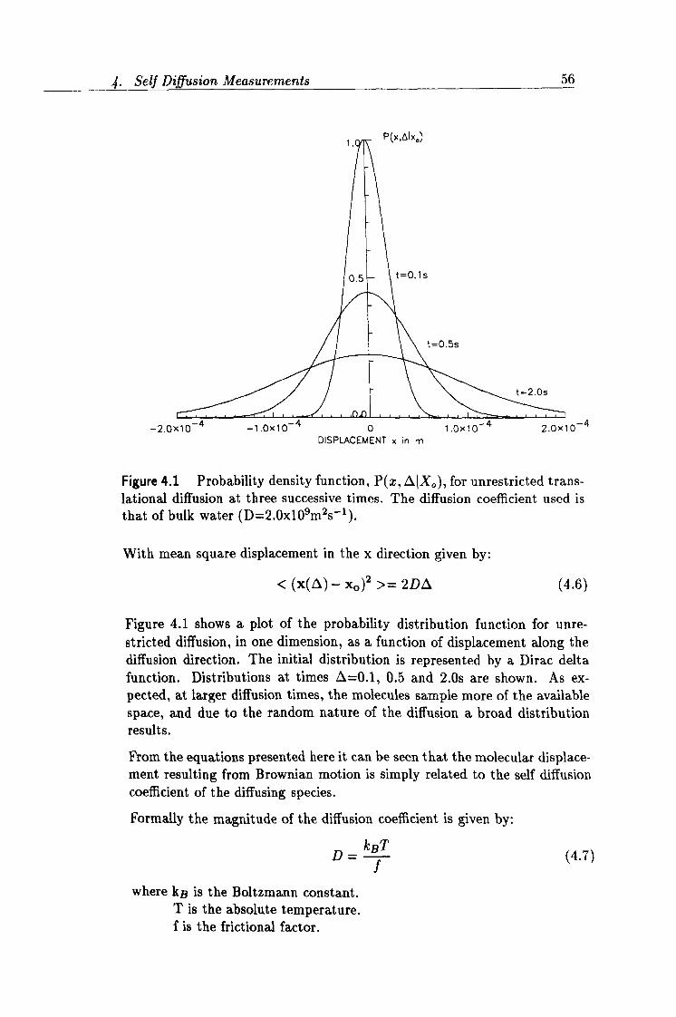
ý. Self Diffusion Measurements 56
P(Y AIV )
-2.0x10⁻⁴ -1.0x10⁻⁴ 0 1.0x10⁻⁴ 2.0x10⁻⁴ DISPLACEMENT x in m
Figure 4.1 Probability density function, P(x, 1 I X, ), for unrestricted trans- lational diffusion at three successive times. The diffusion coefficient used is that of bulk water (D=2.0x10⁹m2s-1).
With mean square displacement in the x direction given by:
< (x(0) - x0)2 >= 2DA (4.6)
Figure 4.1 shows a plot of the probability distribution function for unre- stricted diffusion, in one dimension, as a function of displacement along the diffusion direction. The initial distribution is represented by a Dirac delta function. Distributions at times 0-0.1,0.5 and 2. Os are shown. As ex- pected, at larger diffusion times, the molecules sample more of the available space, and due to the random nature of the diffusion a broad distribution results.
From the equations presented here it can be seen that the molecular displace- ment resulting from Brownian motion is simply related to the self diffusion coefficient of the diffusing species.
Formally the magnitude of the diffusion coefficient is given by:
D=kf (4.7)
where kB is the Boltzmann constant. T is the absolute temperature. f is the frictional factor.
ý. Self Diffusion Measurements 57
For a sphere of radius r in a continuous medium of viscosity q, f is given by the Stokes equation:
f= 6r? 7r
which leads to the Stokes-Einstein equation:
(4.8)
D= kBT (4.9)
For more complex systems, such as polymer solutions, where the polymer chains are far larger than the solvent molecules, more complicated expres- sions are required to define f.
4.2.2 Diffusion in Polymer Solutions
There have been many paradigms proposed to describe the translational molecular diffusion of polymer chains and solvent molecules which occurs within polymer solutions. Many of these models are conflicting and as yet no universal theory exists to describe all such systems, but each proposed theory has its advantages and disadvantages.
Obstruction Models
These models describe polymer chains in solution as slow moving and im- penetrable. This obstruction effect leads to a lengthening of the path length for diffusion (tortuosity) for the solvent molecules, as a result of the presence of the polymer. Hence a reduction in the diffusion coefficient with respect to bulk self diffusion is predicted.
The lattice model is a common approach, and was used by Mackie and Meares [751 for their theory. They proposed that the polymer segments are of equal size to the solvent molecules and a proportion of the lattice sites are inaccessible to the solvent due to the presence of the polymer segments. The resulting reduction in the effective diffusion coefficient of the solvent molecules is given by:
D12 _
ýOp (4.10) Do 1+cpp
where ýOp is the volume fraction of polymer, as defined:
ýPn mp/pp (4.11) E mi/Pt
where m= is the mass of component i. p; is the density of component i.
This model, which holds only for the diffusion of very small solvent molecules, provides a good approximation for a variety of polymer/solvent systems and a large range of polymer concentrations [69,76].
ý. Self Diffusion Measurements 58
Free Volume Models
Free volume models have been widely used for the interpretation of the concentration dependence of small molecules diffusing in polymer matrices. The free volume theory developed by Fujita [2] considers diffusion to involve molecules jumping into voids created by the thermal motion of the molecules. Once again the diffusion coefficient of the solvent is predicted to decrease with increasing polymer concentration, due to the free volume intrinsic to the polymer being much less than that of the solvent. Using this model the diffusion coefficient can be related to the free volume by:
Da exp(-v*/vf) (4.12)
where v* is the characteristic volume required to accommodate the diffusing molecule. vf is the free volume.
The model, which does not apply to aqueous systems, successfully reproduces the concentration dependence of the diffusion for a range of organic solvent- polymer systems [77,781.
Yasuda adapted the free volume theory of diffusion to predict the behaviour in aqueous systems [79]. The reduced diffusion coefficient is a function of the probability of encountering a void of similar size to the cross-section of the diffusing molecule:
D= exp fw 1-11
yp (4.13) Do
where B8 is a measure of the size of the diffusing molecule. f,,, is the free volume contributed by the water.
A plot of ln(D/Do) against 1/1-cpp leads to a linear graph with slope equal to the free volume parameter, B8/f,,,.
A more comprehensive free volume model is the one developed by Vrentas and Duda [80,81,82]. This model describes the diffusion of large solvent molecules and polymer chains more adequately. The disadvantage of this model is that it requires the knowledge of many free volume parameters, and these are not readily available for many polymer/solvent systems.
Hydrodynamic Models
Hydrodynamic models explicitly consider the hydrodynamic interactions be- tween the small solvent molecules and the polymer chains. For example, the diffusion of a spherical probe in the presence of randomly distributed fixed spheres, was given by Cukier as [83]:
D=D. exp(-icR) (4.14)
where R is the radius of the diffusing species. K describes the screening of the hydrodynamic interactions between
4. Self Diffusion Measurements 59
the polymer and the solute. For an ideal polymer K is directly proportional to the polymer concentration [84], while for a swollen chain 'c oc c°"75 [851.
Phillies used a more phenomenological approach to derive his "universal" diffusion equation [3,86], which has a stretched exponential form:
D= Do exp(-ac") (4.15)
where a is related to the size of the diffusant.
v is a characteristic of the system. The equation has shown remarkable success in fitting diffusion data, but
as yet there is no solid physical explanation for the parameters a and v. Phillies proposed that a= R/a,, where a,, is the distance of closest approach between the solvent and the polymer chain.
Scaling Models
In semi-dilute and concentrated polymer solutions the diffusion is influenced by the dynamics of the polymer chains. Scaling concepts developed by de Gennes [87] are often used to understand this behaviour.
The polymer solution is simulated as a series of units of size ý, which is known as the correlation length. Langevin and Rondelez proposed a scaling law for the friction coefficient, f, of a molecule of diameter, d, in a polymer solution: f
=exp(_ (_0 (4.16)
where the correlation length was defined in terms of the polymer concentration by de Gennes [87]:
=R9(ccly=ßc-" (4.17)
where c* is the overlap concentration between dilute and semi-dilute regimes. For small solvent molecules, such as water, the diffusion coefficient can be expressed as:
=exp( )
(4.18) Do
Substituting in the definition of ý leads to: D=
exp (v)
(4 . 19)
This is comparable to the "universal" model (equation 4.15) with a=d/ß.
A recent model by Petit et al. [88], based on the scaling model approach, has proved successful in fitting a range of diffusion data for aqueous and organic solvents of varying sizes, in polymer solutions. The model uses the following equation to fit the experimental data:
D1 (4.20) Do -1+ ac2U
ý. Self Diffusion Measurements 60
where a=Do/k/32 and kß2 and v are the characteristic model parameters.
4.3 NMR Pulsed Field Gradient Theory The translational displacement of molecules can be measured using pulsed field gradient NMR. The pioneering paper on this subject was presented by Stejskal and Tanner [47] in 1965. Since then many other approaches have been proposed to overcome instrumental effects which can influence the measurements, such as background gradients and eddy currents [89,90,91]. It is now possible to confidently measure diffusion coefficients to an accuracy of 1% down to values of approximately 10-9-10-10cm2s'1.
4.3.1 Pulsed Field Gradient Spin Echo Experiment
The pulsed field gradient spin echo experiment consists of the application of a field gradient pulse between the 90° and 180° r. f. pulses and an identical field gradient pulse between the 180° pulse and the spin echo. The pulse sequence is schematically shown in figure 4.2. The first field gradient pulse gives each nuclear spin in the sample a phase shift which is linearly dependent upon its position in the magnetic field gradient at that time, z=0.
For a spin i with position xi at this time, the phase shift is given by:
Oi(0) = yög. x; (0) (4.21)
In this case the phase shift labels the spins in the x-co-ordinate. The 180° pulse followed by the second gradient pulse leads to rephasing of the spins. If diffusion occurs during the time interval, 0, between the two gradient pulses, then each spin will receive a phase shift of different magnitude during the second gradient pulse relative to the first:
O%(A) = 'Yb9, [x1(b) - xi(O)] (4.22)
The consequence of this diffusion is an incomplete refocussing of the nuclear magnetization at a time 2T, and therefore a reduction in the echo amplitude:
In ( Ä(Ö))
j= -y2D [2r3 32 + b2 0-
3\ ) g2 (4.23)
\/
3 +2 72 -by2D (ti + t2) + b(t1 + t2) + 2b2
g" go
where t2=2T-(ti+0+b), i. e. the time between the end of the second gradient pulse and the peak of the spin echo.
As the background gradient, go, approaches zero, only the term in g2 remains and the equation reduces to:
In ` A(O))
= -y2g262D A- 3 6)
(4.24)
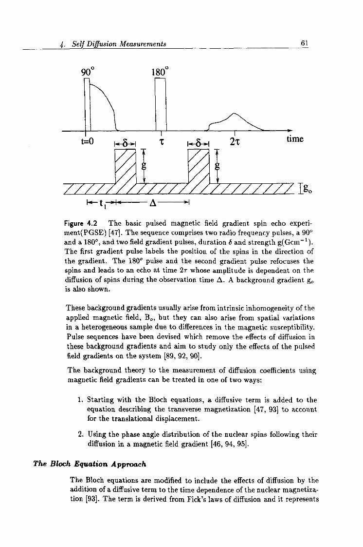
ý. Self Diffusion Measurements 61
t-0 0 ti Zr time
Igo
t 1-ap. 1 E---- 0
Figure 4.2 The basic pulsed magnetic field gradient spin echo experi- ment(PGSE) [471. The sequence comprises two radio frequency pulses, a 90° and a 180°, and two field gradient pulses, duration b and strength g(Gcm-1). The first gradient pulse labels the position of the spins in the direction of the gradient. The 180° pulse and the second gradient pulse refocuses the spins and leads to an echo at time 2r whose amplitude is dependent on the diffusion of spins during the observation time A. A background gradient gp is also shown.
These background gradients usually arise from intrinsic inhomogeneity of the applied magnetic field, Bo, but they can also arise from spatial variations in a heterogeneous sample due to differences in the magnetic susceptibility. Pulse sequences have been devised which remove the effects of diffusion in these background gradients and aim to study only the effects of the pulsed field gradients on the system [89,92,90].
The background theory to the measurement of diffusion coefficients using magnetic field gradients can be treated in one of two ways:
1. Starting with the Bloch equations, a diffusive term is added to the equation describing the transverse magnetization [47,93] to account for the translational displacement.
2. Using the phase angle distribution of the nuclear spins following their diffusion in a magnetic field gradient [46,94,95].
The Bloch Equation Approach
The Bloch equations are modified to include the effects of diffusion by the addition of a diffusive term to the time dependence of the nuclear magnetiza- tion [93]. The term is derived from Fick's laws of diffusion and it represents
90° 1800
¢. Seif Diffusion Measurements 62
the contribution to the rate of change of the magnetization. The modified Bloch equations, in which the magnetization is now a function of both time and spatial co-ordinates, can be written as a single equation:
öMat, t) _ MxB(r, t) -
MA 2Myi) ((M2 M°)k) +V. D. VM
// (4.25)
In the presence of a linear time dependent magnetic field gradient g(t):
Bz = Bo + g(t)"r (4.26)
we can express equation 4.25 as:
8, '(r't) - -i^y (g(t). r), r' +V-D" V1 (4.27)
at where the function O(r, t) is defined by the relationship:
Mx+ iMy = , Oexp (iwot
- , 2) (4.28)
The function O(r, t) represents the amplitude, unattenuated by relaxation, of the complex transverse magnetization in the rotating frame. In this particu- lar case it represents the amplitude having taken account of the contribution of diffusion on the system.
For the 90°-180° spin echo sequence the behaviour of t from the 901 pulse to the time of the echo is given by:
0=A exp (-iyr" (F + (E - 1)f]) (4.29)
where _ +1 for 0<1< T =-1 fort>'r
If A is a function of t only, then:
In (Äßp))i
-y2D [F + (V - 1)f]2 A (4.30)
By substituting in the time dependence of the field gradient it is possible to derive equations for the effect of diffusion on the spin echo amplitude. For the spin-echo experiment this leads to equation 4.24.
The Phase angle approach
The amplitude of the phase sensitive detected NMR spin echo signal along the y' axis of the rotating frame, following the application of a 90° r. f. pulse along the x' axis, may be expressed by:
> (4.31) Myý(2r) = M. G cos[4(2rr)]
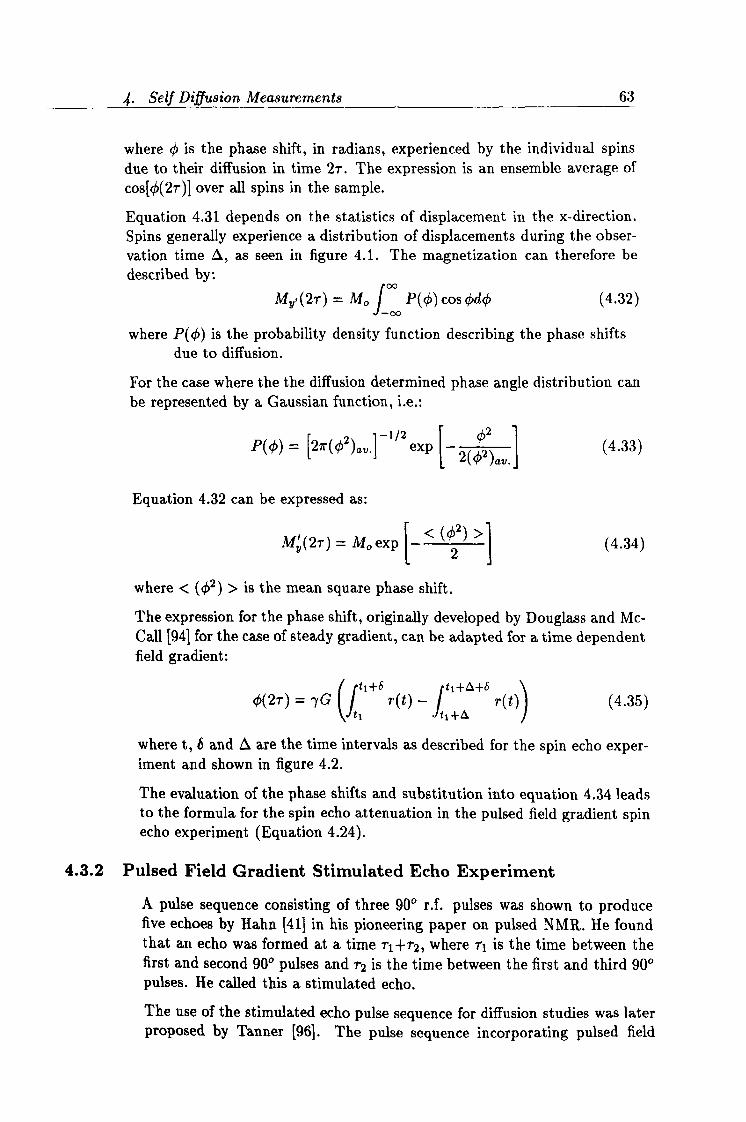
¢, Self Diffusion Measurements 63
where 0 is the phase shift, in radians, experienced by the individual spins due to their diffusion in time 2r. The expression is an ensemble average of cos[«(2r)] over all spins in the sample.
Equation 4.31 depends on the statistics of displacement in the x-direction. Spins generally experience a distribution of displacements during the obser- vation time 0, as seen in figure 4.1. The magnetization can therefore be described by:
00 My, (2-r) = Mo J P(O) cos Odd (4.32) 00
where P(O) is the probability density function describing the phase shifts due to diffusion.
For the case where the the diffusion determined phase angle distribution can be represented by a Gaussian function, i. e.:
2 P(O) _
{21r(2)av. } -1/2 exp - 2(q52)av. (4.33)
Equation 4.32 can be expressed as:
My(2rr) = Mo exp -2 (4.34)
where < (02) > is the mean square phase shift.
The expression for the phase shift, originally developed by Douglass and Mc- Call [94] for the case of steady gradient, can be adapted for a time dependent field gradient:
(it ti+s ti+A+ö 4(2T) = yG
I r(t) -
jtl+a r(t)) (4.35)
where t, 6 and 0 are the time intervals as described for the spin echo exper- iment and shown in figure 4.2.
The evaluation of the phase shifts and substitution into equation 4.34 leads to the formula for the spin echo attenuation in the pulsed field gradient spin echo experiment (Equation 4.24).
4.3.2 Pulsed Field Gradient Stimulated Echo Experiment
A pulse sequence consisting of three 90° r. f. pulses was shown to produce five echoes by Hahn [41] in his pioneering paper on pulsed NMR. He found that an echo was formed at a time r, +r2, where r1 is the time between the first and second 90° pulses and 72 is the time between the first and third 90° pulses. He called this a stimulated echo. The use of the stimulated echo pulse sequence for diffusion studies was later proposed by Tanner [961. The pulse sequence incorporating pulsed field
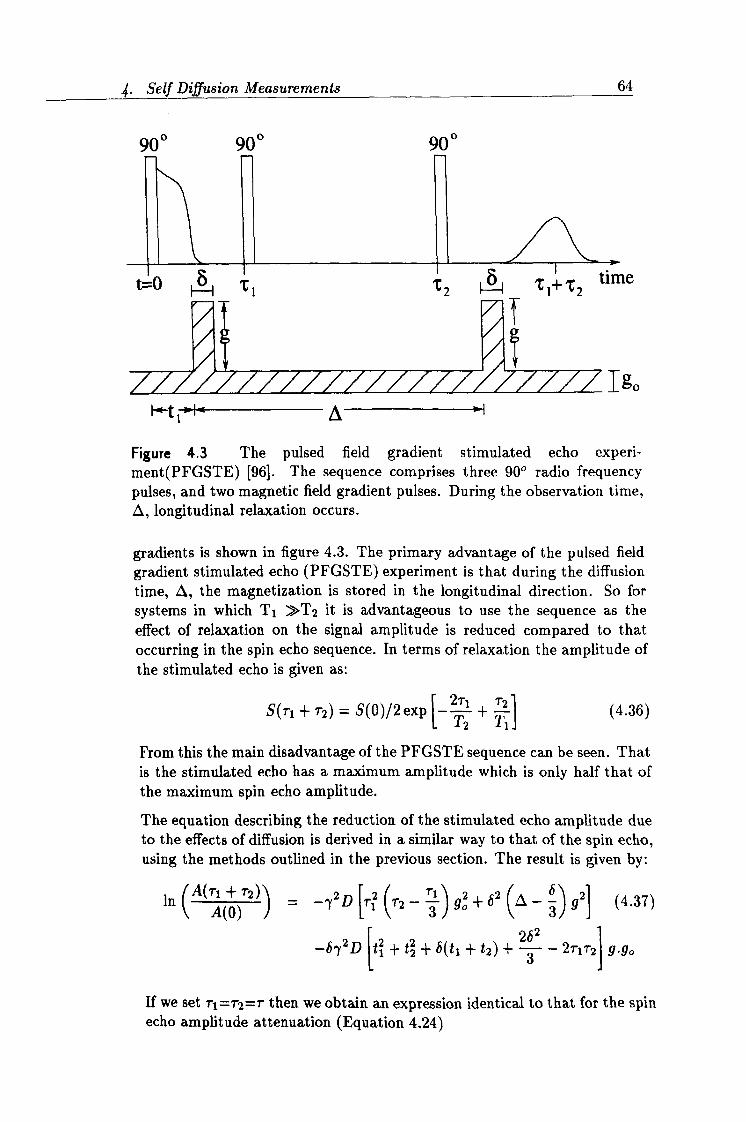
ý. Self Diffusion Measurements 64
90° 90°
t'0 H ý1
900
'C
2N 'c
11 2 time
777 Igo F-t, e
Figure 4.3 The pulsed field gradient stimulated echo experi- ment(PFGSTE) [96]. The sequence comprises three 90° radio frequency
pulses, and two magnetic field gradient pulses. During the observation time, 0, longitudinal relaxation occurs.
gradients is shown in figure 4.3. The primary advantage of the pulsed field gradient stimulated echo (PFGSTE) experiment is that during the diffusion time, 0, the magnetization is stored in the longitudinal direction. So for systems in which T1 »T2 it is advantageous to use the sequence as the effect of relaxation on the signal amplitude is reduced compared to that occurring in the spin echo sequence. In terms of relaxation the amplitude of the stimulated echo is given as:
S(T1 + r2) = S(0)/2exp 1-2, + T2 (4.36) T2- T, 1
From this the main disadvantage of the PFGSTE sequence can be seen. That is the stimulated echo has a maximum amplitude which is only half that of the maximum spin echo amplitude.
The equation describing the reduction of the stimulated echo amplitude due to the effects of diffusion is derived in a similar way to that of the spin echo, using the methods outlined in the previous section. The result is given by:
ln(A(AUTZ)1 _ _y D[r2 (T2- 3) 92 +62
\(0-3j92] (4.37)
A(O) J
a -6y2D t1 + t2 + S(ti + t2) +
23 - 2r-1r2 9.90
If we set ri=rr2=r then we obtain an expression identical to that for the spin echo amplitude attenuation (Equation 4.24)
¢. Self Diffusion Measurements 65
When the background gradient is negligible then equation 4.38 can be sim- plified to:
In (A(2, r))
)= -y2g2ö2D (A-
3) (4.38)
and a conventional plot of ln(A/A(O)) against -ö2y2g2(A-ö/3) returns a linear
plot with a gradient -D.
4.4 Experimental
4.4.1 Gradient calibration
For the measurement of precise self diffusion coefficients it is extremely im- portant to be able to accurately determine the value of the magnetic field gradient strength. Therefore before carrying out any self diffusion exper- iments it is necessary to calibrate the gradients. There are a number of techniques available for achieving this:
1. Use a reference sample with a known value of D [47,96,971. Often a sample of pure water is chosen at a well defined temperature, as D has been well characterized for this substance using various experimental techniques [98,991. In the absence of background gradients a plot of ln[A] against -y2b2D(0-ö/3), results in a linear slope with gradient g2.
2. Use a sample with a well defined geometry. A one dimensional NMR imaging experiment can be carried out which will produce a projection of the sample along the chosen axis with a spatial spread determined by:
x(4.39) 'Yg
where x is the sample dimension along the axis of the applied field gradient
w is the frequency spread covered by the image, calculated from the dwell time. 7= 4257 HzG-1, the magnetogyric ratio in the required units. g is the strength of the magnetic field gradient, units Gcm-1.
To ensure a precise calculation for the value of g using the imaging method, it is important to accurately know the sample length.
3. By studying the lineshape of the spin-echo as a function of an inten- tional mismatch of the gradient pulses [100]. The relative height of the spin echo as a function of the second gradient pulse width is given for a cylindrical sample by:
= 2J1(lRgfsin(a)) S(t)
7Rgcsin(a) (4 40)
where J1 is a first order Bessel function. R is the radius of the cylinder.
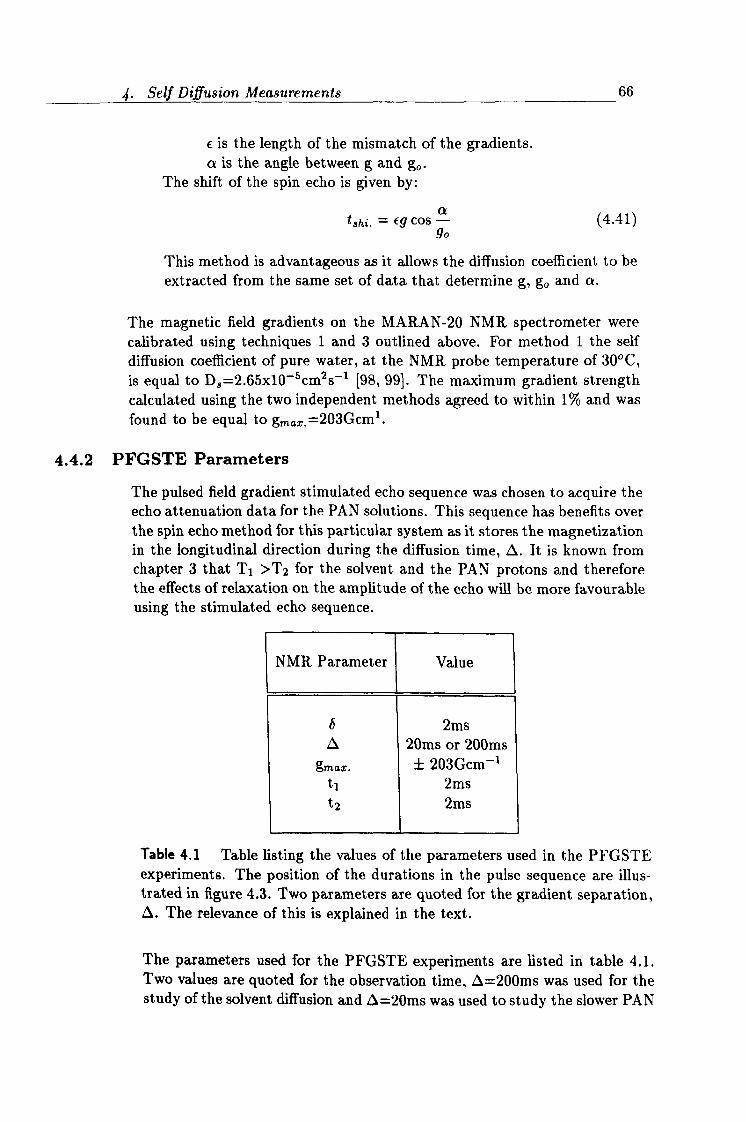
!. Self Diffusion Measurements 66
c is the length of the mismatch of the gradients. a is the angle between g and go.
The shift of the spin echo is given by:
tshi, = IT cos a (4.41) 90
This method is advantageous as it allows the diffusion coefficient to be extracted from the same set of data that determine g, go and a.
The magnetic field gradients on the MARAN-20 NMR spectrometer were calibrated using techniques 1 and 3 outlined above. For method 1 the self diffusion coefficient of pure water, at the NMR probe temperature of 30°C, is equal to D, =2.65x10⁻⁵cm2s-1 [98,991. The maximum gradient strength calculated using the two independent methods agreed to within 1% and was found to be equal to gmar. =203Gcm1.
4.4.2 PFGSTE Parameters
The pulsed field gradient stimulated echo sequence was chosen to acquire the echo attenuation data for the PAN solutions. This sequence has benefits over the spin echo method for this particular system as it stores the magnetization in the longitudinal direction during the diffusion time, A. It is known from chapter 3 that T1 >T2 for the solvent and the PAN protons and therefore the effects of relaxation on the amplitude of the echo will be more favourable using the stimulated echo sequence.
NMR Parameter Value
b 2ms A 20ms or 200ms
gmax. f 203Gcm-1 ti 2ms t2 2ms
Table 4.1 Table listing the values of the parameters used in the PFGSTE experiments. The position of the durations in the pulse sequence are illus- trated in figure 4.3. Two parameters are quoted for the gradient separation, 0. The relevance of this is explained in the text.
The parameters used for the PFGSTE experiments are listed in table 4.1. Two values are quoted for the observation time, 0=200ms was used for the study of the solvent diffusion and L =20ms was used to study the slower PAN
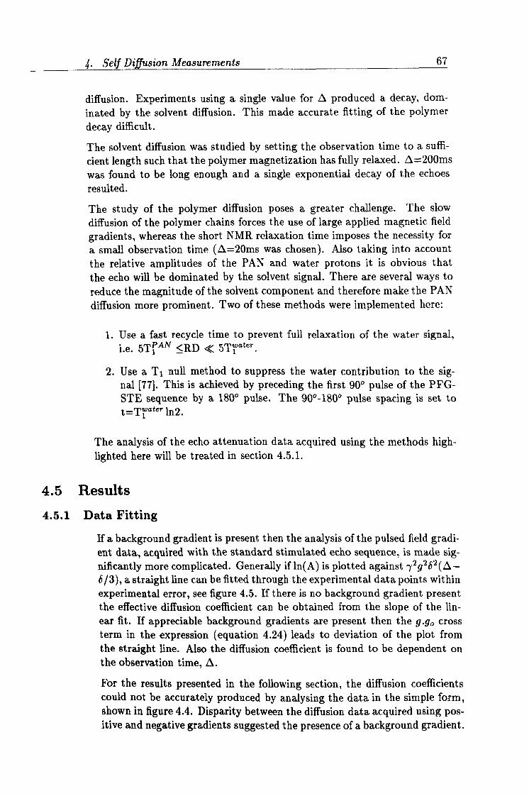
ý. Self Diffusion Measurements 67
diffusion. Experiments using a single value for A produced a decay, dom- inated by the solvent diffusion. This made accurate fitting of the polymer decay difficult.
The solvent diffusion was studied by setting the observation time to a suffi- cient length such that the polymer magnetization has fully relaxed. 0=200ms
was found to be long enough and a single exponential decay of the echoes resulted.
The study of the polymer diffusion poses a greater challenge. The slow diffusion of the polymer chains forces the use of large applied magnetic field
gradients, whereas the short NMR relaxation time imposes the necessity for
a small observation time (A=20ms was chosen). Also taking into account the relative amplitudes of the PAN and water protons it is obvious that the echo will be dominated by the solvent signal. There are several ways to reduce the magnitude of the solvent component and therefore make the PAN diffusion more prominent. Two of these methods were implemented here:
1. Use a fast recycle time to prevent full relaxation of the water signal, <RD « 5T1 ester i. e. 5TPAN
2. Use a Tl null method to suppress the water contribution to the sig- nal [77]. This is achieved by preceding the first 90° pulse of the PFG- STE sequence by a 180° pulse. The 900-1800 pulse spacing is set to t=Ti ester ln2.
The analysis of the echo attenuation data acquired using the methods high- lighted here will be treated in section 4.5.1.
4.5 Results
4.5.1 Data Fitting
If a background gradient is present then the analysis of the pulsed field gradi- ent data, acquired with the standard stimulated echo sequence, is made sig- nificantly more complicated. Generally if ln(A) is plotted against y2g2S2(0- b13), a straight line can be fitted through the experimental data points within experimental error, see figure 4.5. If there is no background gradient present the effective diffusion coefficient can be obtained from the slope of the lin- ear fit. If appreciable background gradients are present then the g. g, cross term in the expression (equation 4.24) leads to deviation of the plot from the straight line. Also the diffusion coefficient is found to be dependent on the observation time, A.
For the results presented in the following section, the diffusion coefficients could not be accurately produced by analysing the data in the simple form, shown in figure 4.4. Disparity between the diffusion data acquired using pos- itive and negative gradients suggested the presence of a background gradient.
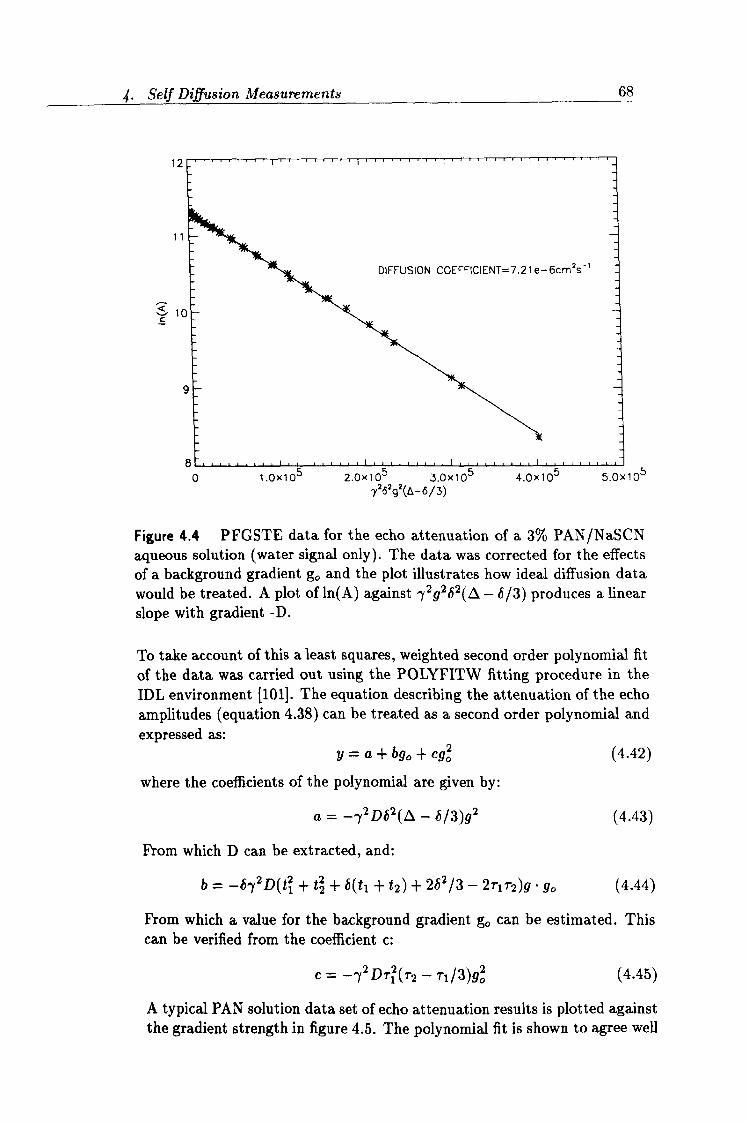
4. Self Diffusion Measurements 68
12
1C c
105 26292 (6- 6/3)
Figure 4.4 PFGSTE data for the echo attenuation of a 3% PAN/NaSCN aqueous solution (water signal only). The data was corrected for the effects of a background gradient go and the plot illustrates how ideal diffusion data would be treated. A plot of ln(A) against y2g2ö2(A - S/3) produces a linear slope with gradient -D.
To take account of this a least squares, weighted second order polynomial fit
of the data was carried out using the POLYFITW fitting procedure in the IDL environment [101]. The equation describing the attenuation of the echo amplitudes (equation 4.38) can be treated as a second order polynomial and expressed as:
y=a+ bgo + ego (4.42)
where the coefficients of the polynomial are given by:
a= -y2DE2(A - ö/3)g2 (4.43)
From which D can be extracted, and:
b= -öy2D(tl + t2 + b(ti + t2) + 262/3 - 2rr1ýr2)9.90 (4.44)
From which a value for the background gradient go can be estimated. This can be verified from the coefficient c:
_ -'y2D7-i (T2 - ri/3)9ö (4.45)
A typical PAN solution data set of echo attenuation results is plotted against the gradient strength in figure 4.5. The polynomial fit is shown to agree well
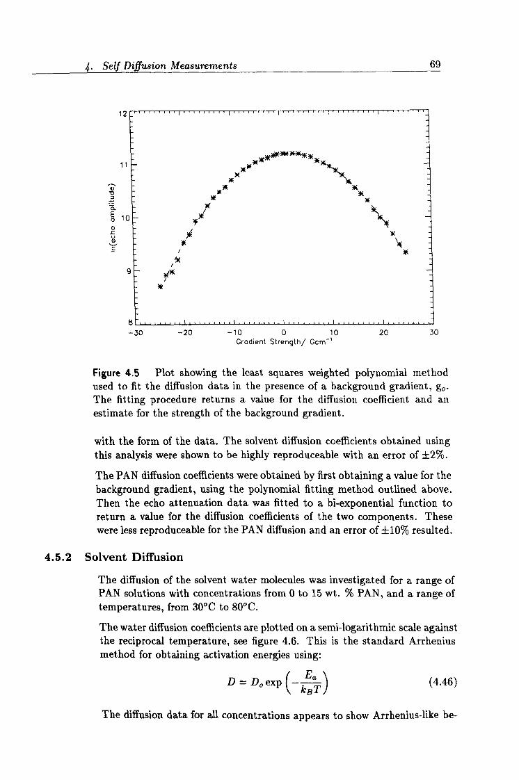
4. Self Diffusion Measurements 69
12
11
ö 1C 0 UU
Figure 4.5 Plot showing the least squares weighted polynomial method used to fit the diffusion data in the presence of a background gradient, go. The fitting procedure returns a value for the diffusion coefficient and an estimate for the strength of the background gradient.
with the form of the data. The solvent diffusion coefficients obtained using this analysis were shown to be highly reproduceable with an error of ±2%.
The PAN diffusion coefficients were obtained by first obtaining a value for the background gradient, using the polynomial fitting method outlined above. Then the echo attenuation data was fitted to a bi-exponential function to return a value for the diffusion coefficients of the two components. These were less reproduceable for the PAN diffusion and an error of ±10% resulted.
4.5.2 Solvent Diffusion
The diffusion of the solvent water molecules was investigated for a range of PAN solutions with concentrations from 0 to 15 wt. % PAN, and a range of temperatures, from 30°C to 80°C.
The water diffusion coefficients are plotted on a semi-logarithmic scale against the reciprocal temperature, see figure 4.6. This is the standard Arrhenius method for obtaining activation energies using:
D. Do exp (- 7, ý (4.46)
a
The diffusion data for all concentrations appears to show Arrhenius-like be-
-30 -20 -10 0 10 20 30 Gradient Strength/ Gcm-'
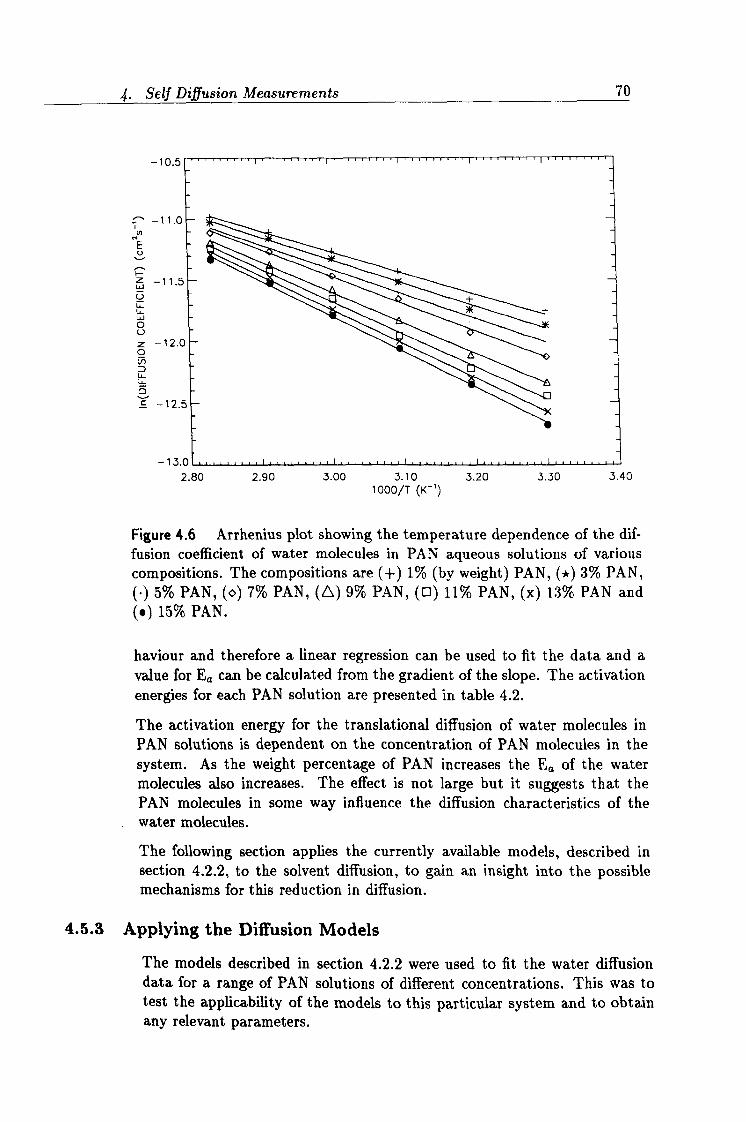
4. Self Diffusion Measurements 70
-10.5
^ -11.0 E U
i? -11.5 U U- U- w 0 U z -12. C 0 L-
M
S -12.:
-13.1 2.80 2.90 3.00 3.10 3.20 3.30 3.40
1000/T (K-')
Figure 4.6 Arrhenius plot showing the temperature dependence of the dif- fusion coefficient of water molecules in PAN aqueous solutions of various compositions. The compositions are (+) 1% (by weight) PAN, (*) 3% PAN, () 5% PAN, (o) 7% PAN, (0) 9% PAN, (0) 11% PAN, (x) 13% PAN and (ý) 15% PAN.
haviour and therefore a linear regression can be used to fit the data and a value for Ea can be calculated from the gradient of the slope. The activation energies for each PAN solution are presented in table 4.2.
The activation energy for the translational diffusion of water molecules in PAN solutions is dependent on the concentration of PAN molecules in the system. As the weight percentage of PAN increases the Ea of the water molecules also increases. The effect is not large but it suggests that the PAN molecules in some way influence the diffusion characteristics of the water molecules.
The following section applies the currently available models, described in section 4.2.2, to the solvent diffusion, to gain an insight into the possible mechanisms for this reduction in diffusion.
4.5.3 Applying the Diffusion Models
The models described in section 4.2.2 were used to fit the water diffusion data for a range of PAN solutions of different concentrations. This was to test the applicability of the models to this particular system and to obtain any relevant parameters.
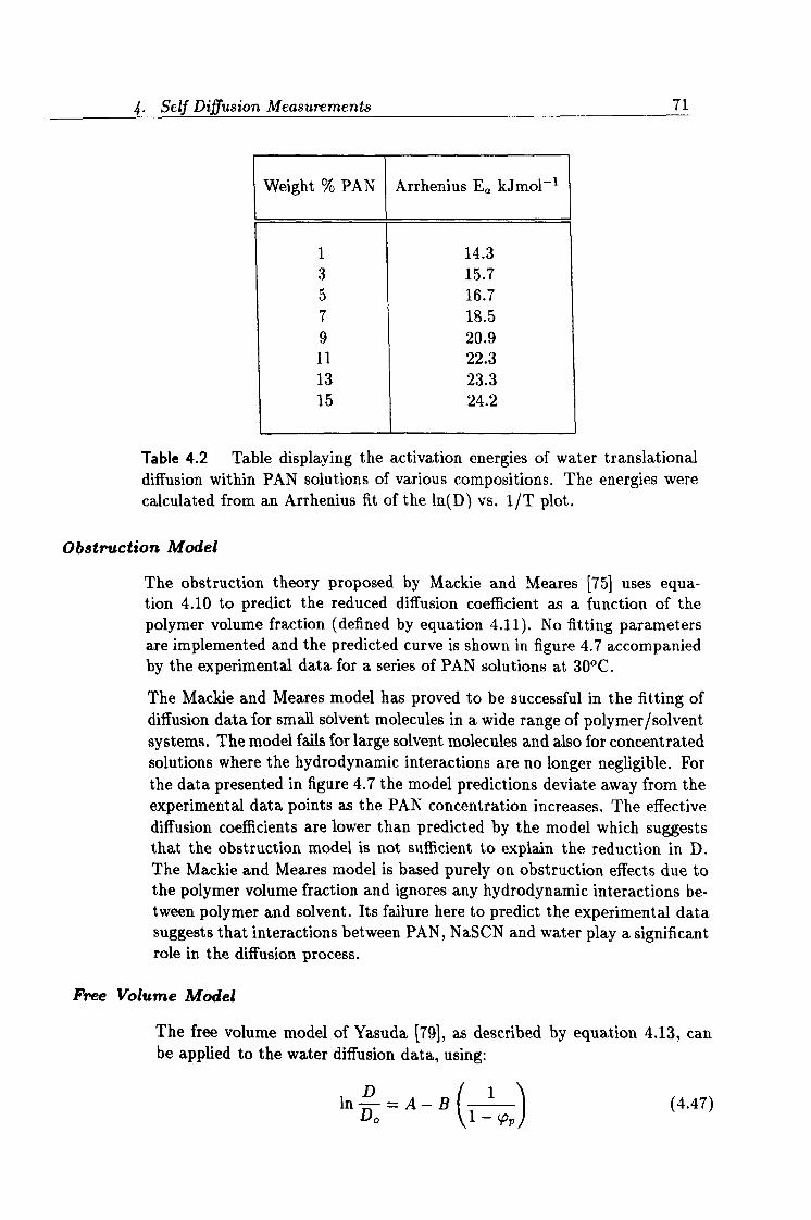
4. Self Diffusion Measurements 71
Weight % PAN Arrhenius Ea, kJmol-1
1 14.3 3 15.7 5 16.7 7 18.5 9 20.9 11 22.3 13 23.3 15 24.2
Table 4.2 Table displaying the activation energies of water translational diffusion within PAN solutions of various compositions. The energies were calculated from an Arrhenius fit of the ln(D) vs. 1/T plot.
Obstruction Model
The obstruction theory proposed by Mackie and Meares [75] uses equa- tion 4.10 to predict the reduced diffusion coefficient as a function of the polymer volume fraction (defined by equation 4.11). No fitting parameters are implemented and the predicted curve is shown in figure 4.7 accompanied by the experimental data for a series of PAN solutions at 30°C.
The Mackie and Meares model has proved to be successful in the fitting of diffusion data for small solvent molecules in a wide range of polymer/solvent systems. The model fails for large solvent molecules and also for concentrated solutions where the hydrodynamic interactions are no longer negligible. For the data presented in figure 4.7 the model predictions deviate away from the experimental data points as the PAN concentration increases. The effective diffusion coefficients are lower than predicted by the model which suggests that the obstruction model is not sufficient to explain the reduction in D. The Mackie and Meares model is based purely on obstruction effects due to the polymer volume fraction and ignores any hydrodynamic interactions be- tween polymer and solvent. Its failure here to predict the experimental data suggests that interactions between PAN, NaSCN and water play a significant role in the diffusion process.
Free Volume Model
The free volume model of Yasuda [79], as described by equation 4.13, can be applied to the water diffusion data, using:
In Do
=A -B1 (4.47) 1-pop
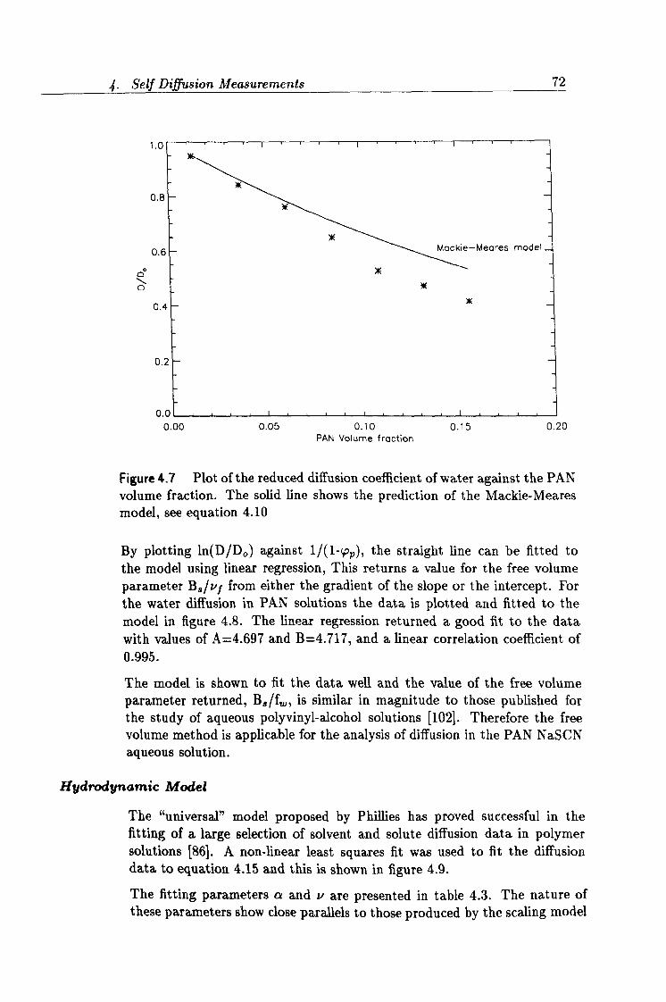
4. Self Diffusion Measurements 72
1.0
0.8
0.6
c
0
0.4
0.1
o. c 0.00 0.05 0.10 0.15 0.20
PAN Volume fraction
X
,
ý, Mackie- model
3ý
Figure 4.7 Plot of the reduced diffusion coefficient of water against the PAN volume fraction. The solid line shows the prediction of the Mackie-Meares model, see equation 4.10
By plotting ln(D/Do) against 1/(1-cpp), the straight line can be fitted to the model using linear regression, This returns a value for the free volume parameter B8lvf from either the gradient of the slope or the intercept. For the water diffusion in PAN solutions the data is plotted and fitted to the model in figure 4.8. The linear regression returned a good fit to the data with values of A=4.697 and B=4.717, and a linear correlation coefficient of 0.995.
The model is shown to fit the data well and the value of the free volume parameter returned, B8/f,,,, is similar in magnitude to those published for the study of aqueous polyvinyl-alcohol solutions [102]. Therefore the free volume method is applicable for the analysis of diffusion in the PAN NaSCN aqueous solution.
Hydrodynamic Model
The "universal" model proposed by Phillies has proved successful in the fitting of a large selection of solvent and solute diffusion data in polymer solutions [86]. A non-linear least squares fit was used to fit the diffusion data to equation 4.15 and this is shown in figure 4.9.
The fitting parameters a and v are presented in table 4.3. The nature of these parameters show close parallels to those produced by the scaling model
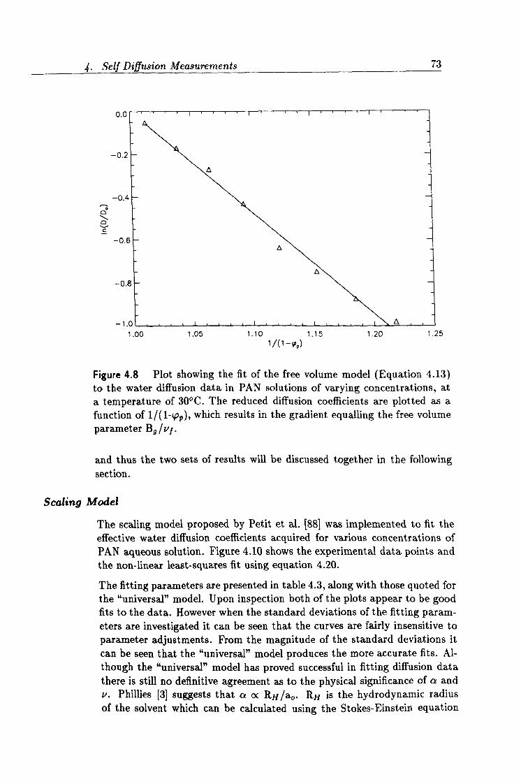
4. Self Diffusion Measurements 73
0.0
-0.2
-0.4 0
0 C
-0.6
-0.8
-1.0 1.00 1.05 1.10 1.15 1.20 1.25
1/(1-app)
Figure 4.8 Plot showing the fit of the free volume model (Equation 4.13) to the water diffusion data in PAN solutions of varying concentrations, at a temperature of 300C. The reduced diffusion coefficients are plotted as a function of 1/(1-cpp), which results in the gradient equalling the free volume parameter Bg/vf.
and thus the two sets of results will be discussed together in the following
section.
Scaling Model
The scaling model proposed by Petit et al. [881 was implemented to fit the effective water diffusion coefficients acquired for various concentrations of PAN aqueous solution. Figure 4.10 shows the experimental data points and the non-linear least-squares fit using equation 4.20.
The fitting parameters are presented in table 4.3, along with those quoted for the "universal" model. Upon inspection both of the plots appear to be good fits to the data. However when the standard deviations of the fitting param- eters are investigated it can be seen that the curves are fairly insensitive to parameter adjustments. From the magnitude of the standard deviations it can be seen that the "universal" model produces the more accurate fits. Al- though the "universal" model has proved successful in fitting diffusion data there is still no definitive agreement as to the physical significance of a and v. Phillies [3] suggests that aa RH/ao. RH is the hydrodynamic radius of the solvent which can be calculated using the Stokes-Einstein equation
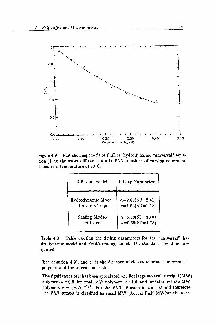
4. Self Diffusion Measurements 74
1.0
0.8
0.6
0 a
0. ý
0.:
Figure 4.9 Plot showing the fit of Phillies' hydrodynamic "universal" equa- tion [3] to the water diffusion data in PAN solutions of varying concentra- tions, at a temperature of 30°C.
Diffusion Model Fitting Parameters
Hydrodynamic Model- a=2.60(SD=2.41) "Universal" eqn. v=1.02(SD=1.52)
Scaling Model- a=5.68(SD=20.8) Petit's eqn. v=0.66(SD=1.78)
Table 4.3 Table quoting the fitting parameters for the "universal" hy- drodynamic model and Petit's scaling model. The standard deviations are quoted.
(See equation 4.9), and ao is the distance of closest approach between the polymer and the solvent molecule
The significance of v has been speculated on. For large molecular weight(MW) polymers v ; 0.5, for small MW polymers v and for intermediate MW polymers v= (MW)-1/4. For the PAN diffusion fit v=1.02 and therefore the PAN sample is classified as small MW (Actual PAN MW(weight aver-
0.01 1-1-1-11-1.11-111, i 0.00 0.10 0.20 0.30 0.40 0.50
Polymer conc. (g/ml)
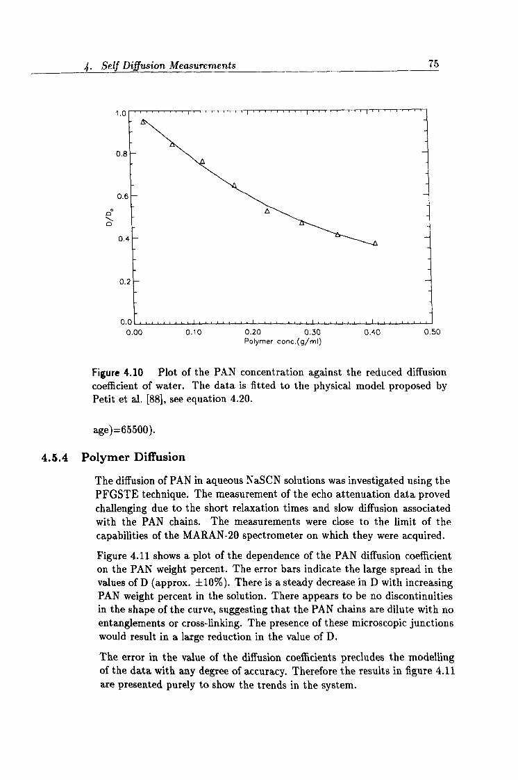
1. Self Diffusion Measurements 75
1.0
0.8
0.6
0 0
0.4
0.1
0.1
0.00 0.10 0.20 0.30 0.40 0.50 Polymer conc. (g/ml)
Figure 4.10 Plot of the PAN concentration against the reduced diffusion
coefficient of water. The data is fitted to the physical model proposed by Petit et al. [881, see equation 4.20.
age)=65500).
4.5.4 Polymer Diffusion
The diffusion of PAN in aqueous NaSCN solutions was investigated using the PFGSTE technique. The measurement of the echo attenuation data proved challenging due to the short relaxation times and slow diffusion associated with the PAN chains. The measurements were close to the limit of the capabilities of the MARAN-20 spectrometer on which they were acquired.
Figure 4.11 shows a plot of the dependence of the PAN diffusion coefficient on the PAN weight percent. The error bars indicate the large spread in the values of D (approx. ±10%). There is a steady decrease in D with increasing PAN weight percent in the solution. There appears to be no discontinuities in the shape of the curve, suggesting that the PAN chains are dilute with no entanglements or cross-linking. The presence of these microscopic junctions would result in a large reduction in the value of D.
The error in the value of the diffusion coefficients precludes the modelling of the data with any degree of accuracy. Therefore the results in figure 4.11 are presented purely to show the trends in the system.
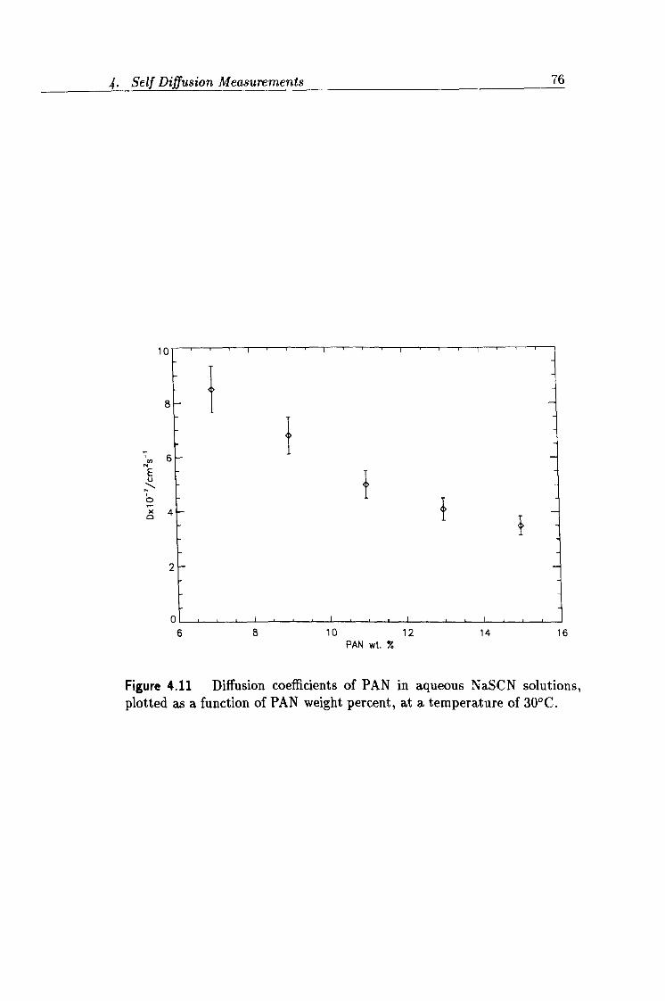
ý. Self Diffusion Measurements 76
10
E U n
O_
X D
PAN wt.
Figure 4.11 Diffusion coefficients of PAN in aqueous NaSCN solutions, plotted as a function of PAN weight percent, at a temperature of 30°C.
6S 10 12 14 16
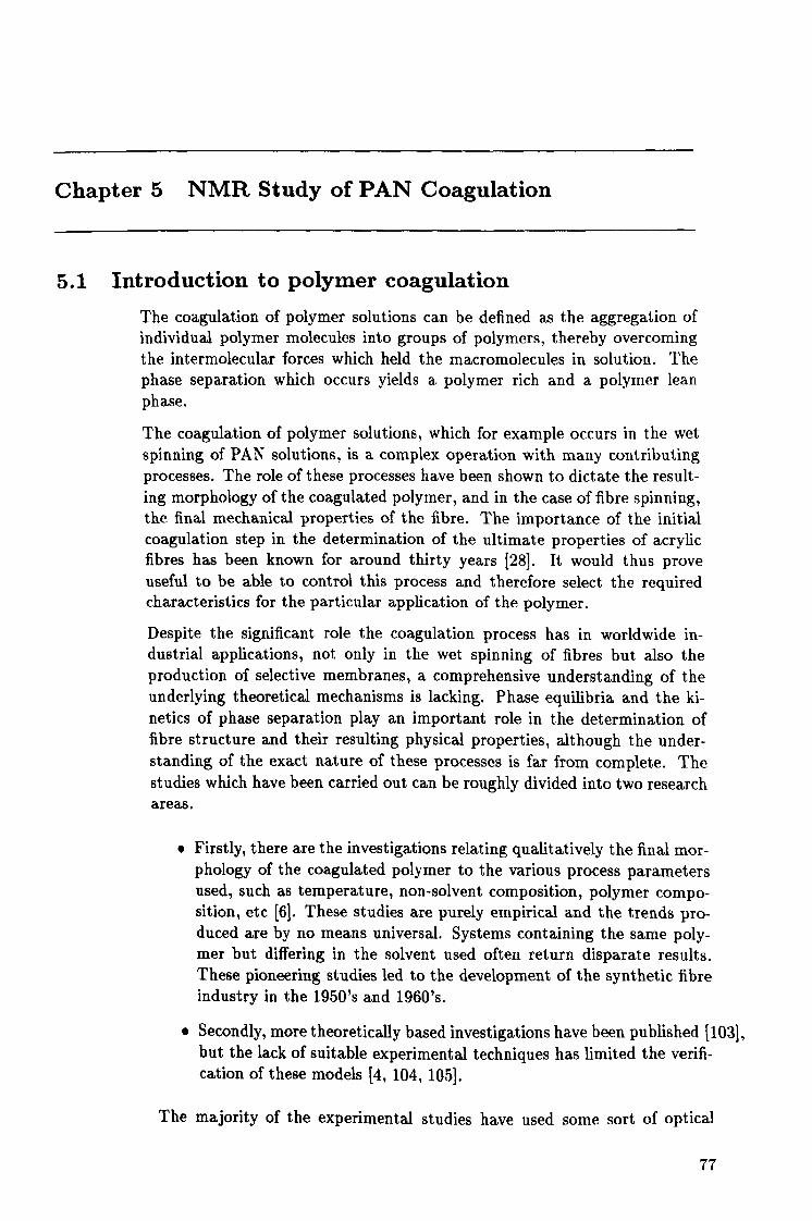
Chapter 5 NMR Study of PAN Coagulation
5.1 Introduction to polymer coagulation The coagulation of polymer solutions can be defined as the aggregation of individual polymer molecules into groups of polymers, thereby overcoming the intermolecular forces which held the macromolecules in solution. The phase separation which occurs yields a polymer rich and a polymer lean phase.
The coagulation of polymer solutions, which for example occurs in the wet spinning of PAN solutions, is a complex operation with many contributing processes. The role of these processes have been shown to dictate the result- ing morphology of the coagulated polymer, and in the case of fibre spinning, the final mechanical properties of the fibre. The importance of the initial coagulation step in the determination of the ultimate properties of acrylic fibres has been known for around thirty years [28]. It would thus prove useful to be able to control this process and therefore select the required characteristics for the particular application of the polymer.
Despite the significant role the coagulation process has in worldwide in- dustrial applications, not only in the wet spinning of fibres but also the production of selective membranes, a comprehensive understanding of the underlying theoretical mechanisms is lacking. Phase equilibria and the ki- netics of phase separation play an important role in the determination of fibre structure and their resulting physical properties, although the under- standing of the exact nature of these processes is far from complete. The studies which have been carried out can be roughly divided into two research areas.
" Firstly, there are the investigations relating qualitatively the final mor- phology of the coagulated polymer to the various process parameters used, such as temperature, non-solvent composition, polymer compo- sition, etc [6]. These studies are purely empirical and the trends pro- duced are by no means universal. Systems containing the same poly- mer but differing in the solvent used often return disparate results. These pioneering studies led to the development of the synthetic fibre industry in the 1950's and 1960's.
" Secondly, more theoretically based investigations have been published [103}, but the lack of suitable experimental techniques has limited the verifi- cation of these models [4,104,105].
The majority of the experimental studies have used some sort of optical
77
5. NMR Study of PAN Coagulation
INCREASING
COAGULATION TIME
Uncoagulated polymer solution.
" Coagulated polymer, porous in nature.
0 Dense skin of coagulated polymer.
ýý
Figure 5.1 Measuring the growth of the coagulated layer as a function of time by optical methods is one technique for obtaining quantitative infor-
mation about the coagulation process. Here we see the development of the internal fibre structure as a function of coagulation time. Notice the dense
skin which is initially formed. This is characteristic of most wet spinning systems.
technique to monitor the growth of the coagulated polymer in the fibre [106], see figure 5.1. The development of the boundary layer as a function of time has been shown to exhibit a square root of time relationship and therefore Fickian behaviour for infinite systems [27].
Nuclear magnetic resonance has proven to be a useful tool for studying the change in mobilities of NMR active species in a wide range of research fields. In the case of a polymer precipitating out of solution the variation in relax- ation times will reflect a change in the motional properties and environment of the polymer chains. The transverse relaxation time associated with pro- tons attached to the backbone chain will change considerably as the polymer changes from a mobile random coil in solution to a more rigid species as it is coagulated. This can give us a handle on this particular process. By studying this change as a function of time it is possible to obtain quantita- tive information about the rate of polymer coagulation. This method has been used successively in probing the kinetics of the crystallization of cis-1,4- polybutadiene [107], polydimethylsiloxane [108] and polyetherimide [109].
In this chapter it will be outlined how nuclear magnetic resonance can be used to study the coagulation process of PAN from aqueous NaSCN solutions and produce useful quantitative data.
5. NMR Study of PAN Coagulation 79
5.2 Theoretical
The complicated phenomena involved in the coagulation of polymer solu- tions, such as those taking place in the wet spinning process, can be roughly divided into two contributing aspects. These are (i) the thermodynamics of the phase separation and (ii) the kinetics involved in the diffusive inter- change of solvent and non-solvent. The role of both of these will be described in more detail here.
5.2.1 Phase separation
The phase separation of a polymer solution is a process whereby a homoge- neous solution is transformed into a two phase system consisting of a polymer rich and polymer lean phase. This transformation is generally achieved by one of two main methods.
Thermally induced phase separation
Thermally induced phase separation involves cooling a polymer solution be- low its critical solution temperature and thus crossing the phase boundary. This is best illustrated using a temperature-concentration phase diagram, see figure 5.2.
The dominant factor in determining the mechanism of this process, and ultimately the morphology of the polymer, is the cooling rate. Fast cooling results in spinodal decomposition, whereas if the cooling rate is slow enough for the formation of nuclei the solution is dominated by a nucleation and growth mechanism [110].
Nucleation and growth is associated with metastability and the existence of an energy barrier between the two regimes. The prerequisite for nucleation and growth is the formation of an initial nucleus. This will grow with time and the domains tend to be spherical in shape. Spinodal decomposition occurs in the unstable region where a negligible energy barrier is present. The system therefore spontaneously separates into two phases which tend to be cylindrical in shape. The thermodynamics of a polymer system tend to be dominated by the free energy of mixing. This parameter dictates whether the solution remains homogeneous or separates into two phases upon thermal change. Flory- Huggins theory is a good starting point for predicting these effects using phase diagrams [111,112,113].
The Gibbs free energy of mixing, AGm, consists of enthalpic and entropic contributions:
OG"'' = OH"` - TOS' (5.1)
where OG' <0 for spontaneous mixing to occur.
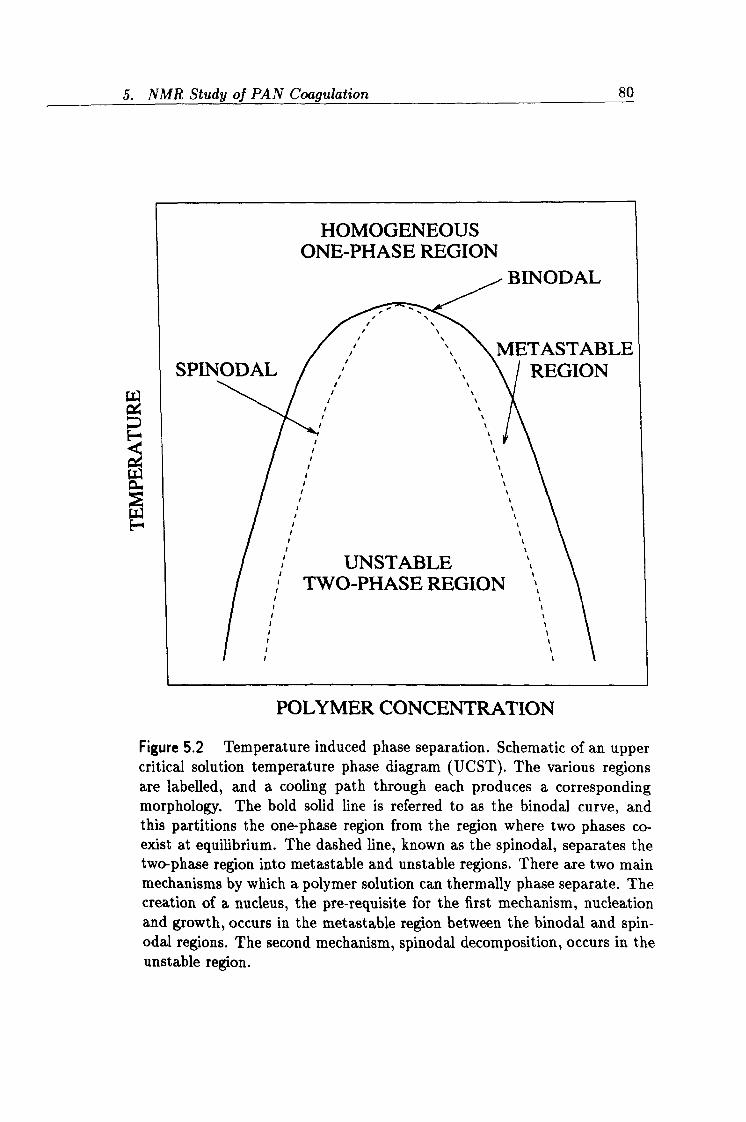
5. NMR Study of PAN Coagulation 80
HOMOGENEOUS ONE-PHASE REGION
BINODAL
E-+
W a w H
METASTABLE SPINODAL REGION
UNSTABLE TWO-PHASE REGION ,
POLYMER CONCENTRATION
Figure 5.2 Temperature induced phase separation. Schematic of an upper critical solution temperature phase diagram (UCST). The various regions are labelled, and a cooling path through each produces a corresponding morphology. The bold solid line is referred to as the binodal curve, and this partitions the one-phase region from the region where two phases co- exist at equilibrium. The dashed line, known as the spinodal, separates the two-phase region into metastable and unstable regions. There are two main mechanisms by which a polymer solution can thermally phase separate. The creation of a nucleus, the pre-requisite for the first mechanism, nucleation and growth, occurs in the metastable region between the binodal and spin- odal regions. The second mechanism, spinodal decomposition, occurs in the unstable region.
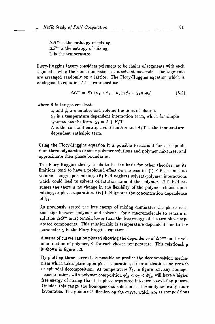
5. NMR Study of PAN Coagulation 81
iH' is the enthalpy of mixing. OS' is the entropy of mixing. T is the temperature.
Flory-Huggins theory considers polymers to be chains of segments with each segment having the same dimensions as a solvent molecule. The segments are arranged randomly on a lattice. The Flory-Huggins equation which is analogous to equation 5.1 is expressed as:
OG' = RT (nl In 01 + n211102 + X, ni 02) (5.2)
where R is the gas constant. n; and q5 are number and volume fractions of phase i. Xi is a temperature dependent interaction term, which for simple systems has the form, X, =A+ BIT. A is the constant entropic contribution and B/T is the temperature dependent enthalpic term.
Using the Flory-Huggins equation it is possible to account for the equilib- rium thermodynamics of some polymer solutions and polymer mixtures, and approximate their phase boundaries.
The Flory-Huggins theory tends to be the basis for other theories, as its limitions tend to have a profound effect on the results: (1) F-H assumes no volume change upon mixing. (ii) F-H neglects solvent-polymer interactions which could lead to solvent orientation around the polymer. (iii) F-H as- sumes the there is no change in the flexibilty of the polymer chains upon mixing, or phase separation. (iv) F-H ignores the concentration dependence of Xl.
As previously stated the free energy of mixing dominates the phase rela- tionships between polymer and solvent. For a macromolecule to remain in solution AGm must remain lower than the free energy of the two phase sep- arated components. This relationship is temperature dependent due to the parameter X in the Flory-Huggins equation.
A series of curves can be plotted showing the dependence of OG"' on the vol- ume fraction of polymer, 0, for each chosen temperature. This relationship is shown in figure 5.3.
By plotting these curves it is possible to predict the decomposition mecha- nism which takes place upon phase separation, either nucleation and growth or spinodal decomposition. At temperature T2, in figure 5.3, any homoge- neous solution, with polymer composition X26 < 02 < O2b, will have a higher free energy of mixing than if it phase separated into two co-existing phases. Outside this range the homogeneous solution is thermodynamically more favourable. The points of inflection on the curve, which are at compositions
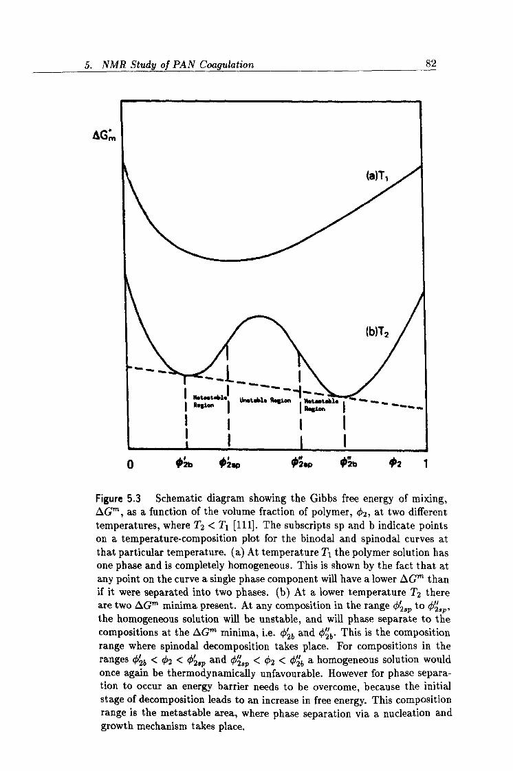
5. NMR Study of PAN Coagulation 82
AGm
(a)TI
(b)T2
1") Unstable %ion ( I. (- " .., -ýý Rftlon .ý
0 Orb ýiw o sp
4ib #2 1
Figure 5.3 Schematic diagram showing the Gibbs free energy of mixing, AGm, as a function of the volume fraction of polymer, 02, at two different temperatures, where T2 < Ti [111]. The subscripts sp and b indicate points on a temperature-composition plot for the binodal and spinodal curves at that particular temperature. (a) At temperature Tl the polymer solution has one phase and is completely homogeneous. This is shown by the fact that at any point on the curve a single phase component will have a lower LSG'' than if it were separated into two phases. (b) At a lower temperature T2 there are two OG" minima present. At any composition in the range 4 28p to 02sp, the homogeneous solution will be unstable, and will phase separate to the compositions at the AG' minima, i. e. 0'2b and ¢2b. This is the composition range where spinodal decomposition takes place. For compositions in the ranges ¢2b < 02 < O2ap and 02ap < 02 < 0'2b a homogeneous solution would once again be thermodynamically unfavourable. However for phase separa- tion to occur an energy barrier needs to be overcome, because the initial stage of decomposition leads to an increase in free energy. This composition range is the metastable area, where phase separation via a nucleation and growth mechanism takes place.
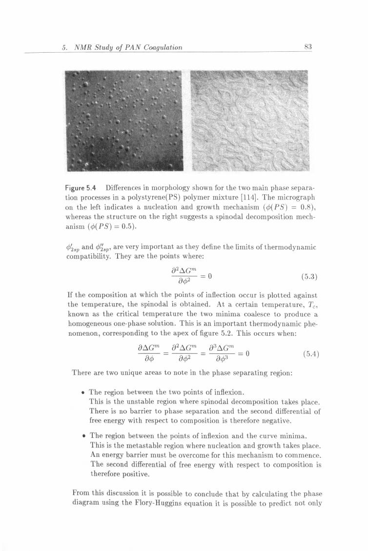
i. NMR Study of PAN Coagulation 83
_, ý
,_ - ýýý. ý1
L, ý ý Lý
+,
aý
ýc
4L AL,
Figure 5.4 Differences in morphology shown for the two main phase separa- tion processes in a polystyrene(PS) polymer mixture [114]. The micrograph on the left indicates a nucleation and growth mechanism (g5(PS) = 0.8),
whereas the structure on the right suggests a spinodal decomposition mech- anism (B(PS) = 0.5).
02sp and O'2sp, are very important as they define the limits of thermodynamic compatibility. They are the points where:
102 AGB" a02 =0 (5.3)
If the composition at which the points of inflection occur is plotted against the temperature, the spinodal is obtained. At a certain temperature, T, known as the critical temperature the two minima coalesce to produce a homogeneous one-phase solution. This is an important thermodynamic phe- nomenon, corresponding to the apex of figure 5.2. This occurs when:
_OG' a2 AG' ä30G'
There are two unique areas to note in the phase separating region:
(5.4)
" The region between the two points of inflexion. This is the unstable region where spinodal decomposition takes place. There is no barrier to phase separation and the second differential of free energy with respect to composition is therefore negative.
" The region between the points of inflexion and the curve minima. This is the metastable region where nucleation and growth takes place. An energy barrier must be overcome for this mechanism to commence. The second differential of free energy with respect to composition is therefore positive.
From this discussion it is possible to conclude that by calculating the phase diagram using the Flory-Huggins equation it is possible to predict not only
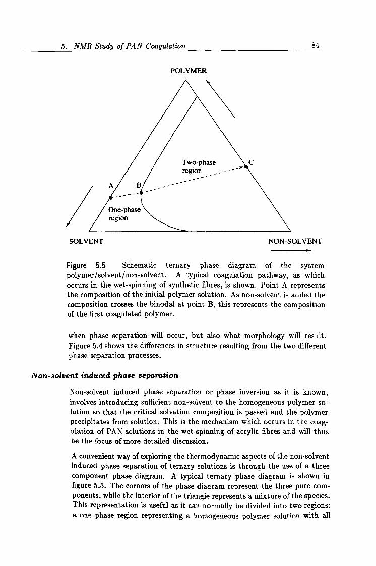
5. NMR Study of PAN Coagulation 84
POLYMER
/ SOLVENT NON-SOLVENT
Figure 5.5 Schematic ternary phase diagram of the system polymer/solvent/non-solvent. A typical coagulation pathway, as which occurs in the wet-spinning of synthetic fibres, is shown. Point A represents the composition of the initial polymer solution. As non-solvent is added the composition crosses the binodal at point B, this represents the composition of the first coagulated polymer.
when phase separation will occur, but also what morphology will result. Figure 5.4 shows the differences in structure resulting from the two different phase separation processes.
Non-solvent induced phase separation
Non-solvent induced phase separation or phase inversion as it is known, involves introducing sufficient non-solvent to the homogeneous polymer so- lution so that the critical solvation composition is passed and the polymer precipitates from solution. This is the mechanism which occurs in the coag- ulation of PAN solutions in the wet-spinning of acrylic fibres and will thus be the focus of more detailed discussion.
A convenient way of exploring the thermodynamic aspects of the non-solvent induced phase separation of ternary solutions is through the use of a three component phase diagram. A typical ternary phase diagram is shown in figure 5.5. The corners of the phase diagram represent the three pure com- ponents, while the interior of the triangle represents a mixture of the species. This representation is useful as it can normally be divided into two regions: a one phase region representing a homogeneous polymer solution with all
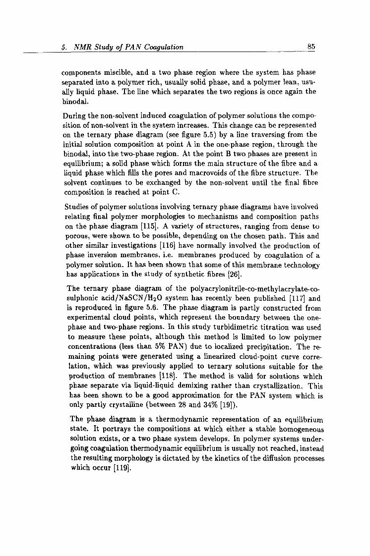
5. NMR Study of PAN Coagulation 85
components miscible, and a two phase region where the system has phase separated into a polymer rich, usually solid phase, and a polymer lean, usu- ally liquid phase. The line which separates the two regions is once again the binodal.
During the non-solvent induced coagulation of polymer solutions the compo- sition of non-solvent in the system increases. This change can be represented on the ternary phase diagram (see figure 5.5) by a line traversing from the initial solution composition at point A in the one-phase region, through the binodal, into the two-phase region. At the point B two phases are present in equilibrium; a solid phase which forms the main structure of the fibre and a liquid phase which fills the pores and macrovoids of the fibre structure. The solvent continues to be exchanged by the non-solvent until the final fibre composition is reached at point C.
Studies of polymer solutions involving ternary phase diagrams have involved relating final polymer morphologies to mechanisms and composition paths on the phase diagram [115]. A variety of structures, ranging from dense to porous, were shown to be possible, depending on the chosen path. This and other similar investigations [116] have normally involved the production of phase inversion membranes, i. e. membranes produced by coagulation of a polymer solution. It has been shown that some of this membrane technology has applications in the study of synthetic fibres [26].
The ternary phase diagram of the polyacrylonitrile-co-methylacrylate-co- sulphonic acid/NaSCN/H20 system has recently been published [117] and is reproduced in figure 5.6. The phase diagram is partly constructed from experimental cloud points, which represent the boundary between the one- phase and two-phase regions. In this study turbidimetric titration was used to measure these points, although this method is limited to low polymer concentrations (less than 5% PAN) due to localized precipitation. The re- maining points were generated using a linearized cloud-point curve corre- lation, which was previously applied to ternary solutions suitable for the production of membranes [118]. The method is valid for solutions which phase separate via liquid-liquid demixing rather than crystallization. This has been shown to be a good approximation for the PAN system which is only partly crystalline (between 28 and 34% [19]).
The phase diagram is a thermodynamic representation of an equilibrium state. It portrays the compositions at which either a stable homogeneous solution exists, or a two phase system develops. In polymer systems under- going coagulation thermodynamic equilibrium is usually not reached, instead the resulting morphology is dictated by the kinetics of the diffusion processes which occur [119].
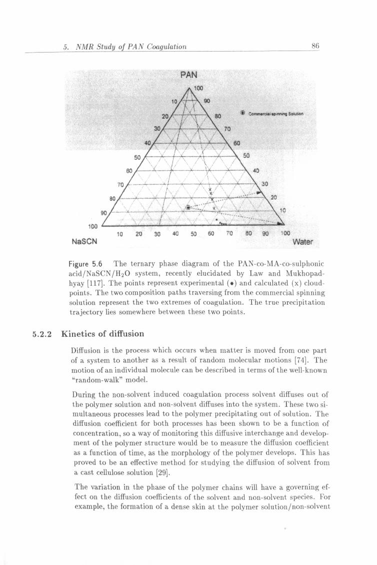
5. NMR Study of PAN Coagulation 86
PAN 100
10 t go
20 - -' ---- 80 ý. OI+ins c.. w mw g solution
30
ot!
70
40 -`- 60
50 50
80 -_ 40
70 _- .__. _ ... ,- , "- -*
_; -. V' '. 30 rx rrZ.
20
90 10
100 10 20 30 40 50 60 70 80 90 100
NaSCN Water
Figure 5.6 The ternary phase diagram of the PAN- co-MA-co-sulphonic acid/NaSCN/H20 system, recently elucidated by Law and Mukhopad- hyay [117]. The points represent experimental (. ) and calculated (x) cloud- points. The two composition paths traversing from the commercial spinning solution represent the two extremes of coagulation. The true precipitation trajectory lies somewhere between these two points.
5.2.2 Kinetics of diffusion
Diffusion is the process which occurs when matter is moved from one part of a system to another as a result of random molecular motions [74]. The
motion of an individual molecule can be described in terms of the well-known "random-walk" model.
During the non-solvent induced coagulation process solvent diffuses out of the polymer solution and non-solvent diffuses into the system. These two si- multaneous processes lead to the polymer precipitating out of solution. The diffusion coefficient for both processes has been shown to be a function of concentration, so a way of monitoring this diffusive interchange and develop- ment of the polymer structure would be to measure the diffusion coefficient as a function of time, as the morphology of the polymer develops. This has proved to be an effective method for studying the diffusion of solvent from a cast cellulose solution [29].
The variation in the phase of the polymer chains will have a governing ef- fect on the diffusion coefficients of the solvent and non-solvent species. For example, the formation of a dense skin at the polymer solution/non-solvent
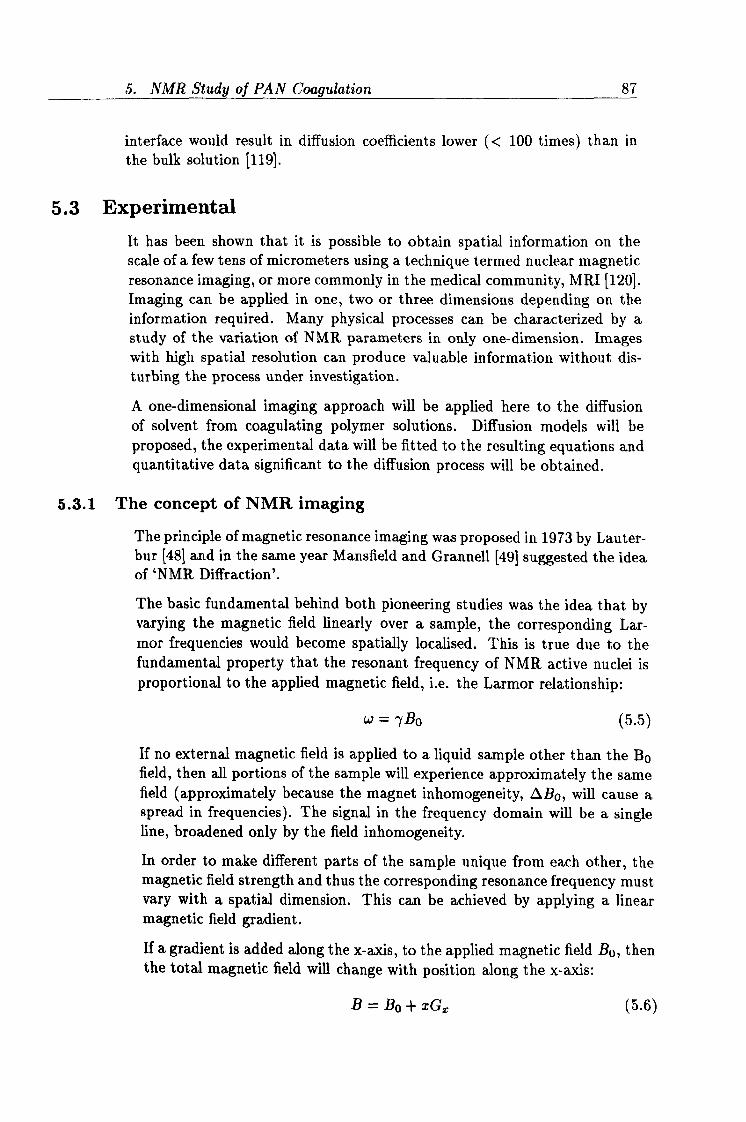
5. NMR Study of PAN Coagulation 87
interface would result in diffusion coefficients lower (< 100 times) than in the bulk solution [119].
5.3 Experimental
It has been shown that it is possible to obtain spatial information on the scale of a few tens of micrometers using a technique termed nuclear magnetic resonance imaging, or more commonly in the medical community, MRI [120]. Imaging can be applied in one, two or three dimensions depending on the information required. Many physical processes can be characterized by a study of the variation of NMR parameters in only one-dimension. Images with high spatial resolution can produce valuable information without dis- turbing the process under investigation.
A one-dimensional imaging approach will be applied here to the diffusion of solvent from coagulating polymer solutions. Diffusion models will be proposed, the experimental data will be fitted to the resulting equations and quantitative data significant to the diffusion process will be obtained.
5.3.1 The concept of NMR imaging
The principle of magnetic resonance imaging was proposed in 1973 by Lauter- bur [48] and in the same year Mansfield and Grannell [49] suggested the idea of `NMR Diffraction'.
The basic fundamental behind both pioneering studies was the idea that by varying the magnetic field linearly over a sample, the corresponding Lar- mor frequencies would become spatially localised. This is true due to the fundamental property that the resonant frequency of NMR active nuclei is proportional to the applied magnetic field, i. e. the Larmor relationship:
w=7Bo (5.5)
If no external magnetic field is applied to a liquid sample other than the Bo field, then all portions of the sample will experience approximately the same field (approximately because the magnet inhomogeneity, AB0, will cause a spread in frequencies). The signal in the frequency domain will be a single line, broadened only by the field inhomogeneity.
In order to make different parts of the sample unique from each other, the magnetic field strength and thus the corresponding resonance frequency must vary with a spatial dimension. This can be achieved by applying a linear magnetic field gradient.
If a gradient is added along the x-axis, to the applied magnetic field Bo, then the total magnetic field will change with position along the x-axis:
B= B0+xG, (5.6)
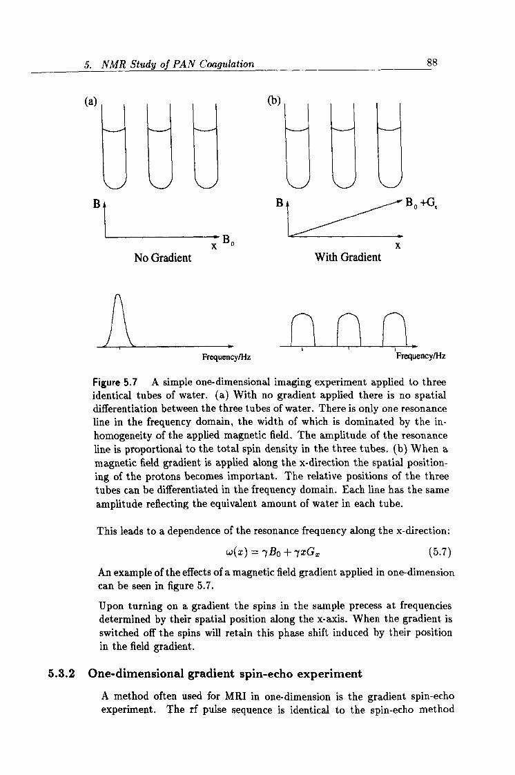
5. NMR Study of PAN Coagulation 88
(a) ý\lý del
V B
xBo No Gradient
Frequency/Hz
B Bo +G,.
With Gradient
Frequency/Hz
Figure 5.7 A simple one-dimensional imaging experiment applied to three identical tubes of water. (a) With no gradient applied there is no spatial differentiation between the three tubes of water. There is only one resonance line in the frequency domain, the width of which is dominated by the in- homogeneity of the applied magnetic field. The amplitude of the resonance line is proportional to the total spin density in the three tubes. (b) When a magnetic field gradient is applied along the x-direction the spatial position- ing of the protons becomes important. The relative positions of the three tubes can be differentiated in the frequency domain. Each line has the same amplitude reflecting the equivalent amount of water in each tube.
This leads to a dependence of the resonance frequency along the x-direction:
w(x) = yBo + yxG3, (5.7) An example of the effects of a magnetic field gradient applied in one-dimension can be seen in figure 5.7.
Upon turning on a gradient the spins in the sample precess at frequencies determined by their spatial position along the x-axis. When the gradient is switched off the spins will retain this phase shift induced by their position in the field gradient.
5.3.2 One-dimensional gradient spin-echo experiment A method often used for MRI in one-dimension is the gradient spin-echo experiment. The rf pulse sequence is identical to the spin-echo method
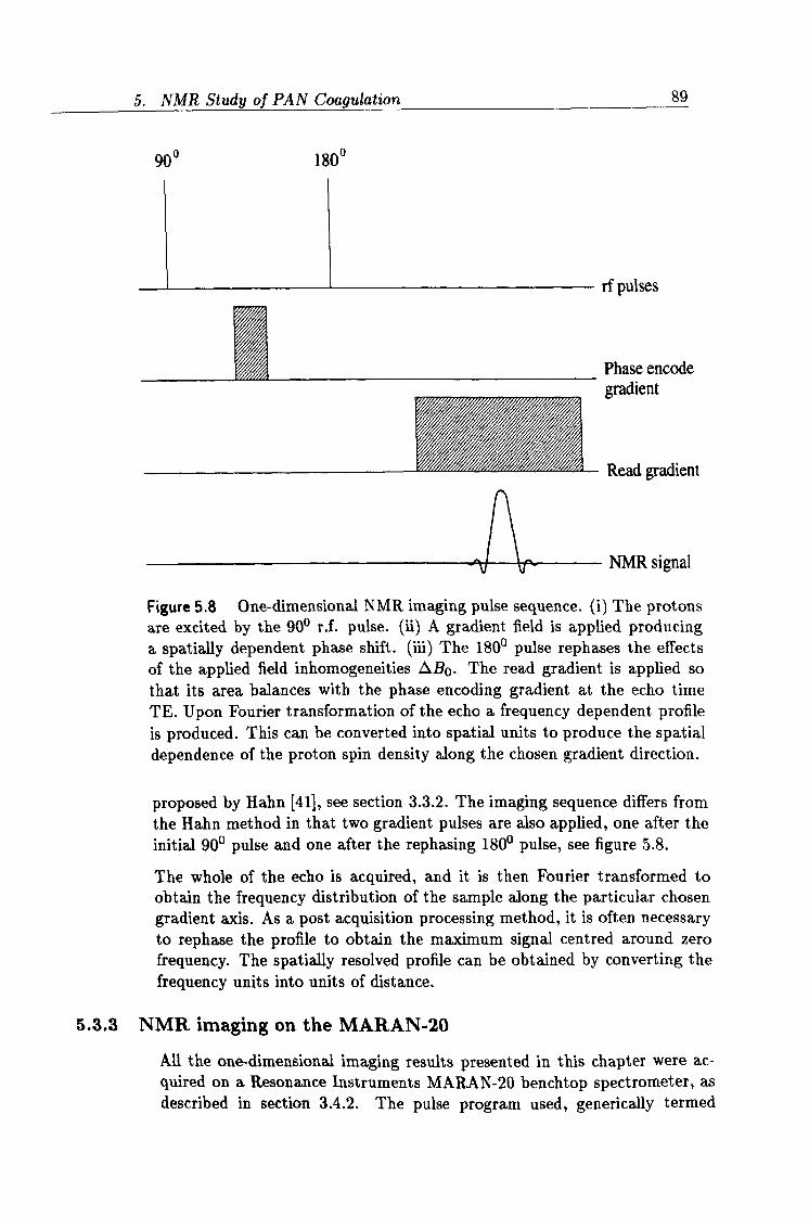
5. NMR Study of PAN Coagulation 89
900 1800
rf pulses
Phase encode gradient
Read gradient
NMR signal
Figure 5.8 One-dimensional NMR imaging pulse sequence. (i) The protons are excited by the 90° r. f. pulse. (ii) A gradient field is applied producing a spatially dependent phase shift. (iii) The 1800 pulse rephases the effects of the applied field inhomogeneities ABO. The read gradient is applied so that its area balances with the phase encoding gradient at the echo time TE. Upon Fourier transformation of the echo a frequency dependent profile is produced. This can be converted into spatial units to produce the spatial dependence of the proton spin density along the chosen gradient direction.
proposed by Hahn [411, see section 3.3.2. The imaging sequence differs from the Hahn method in that two gradient pulses are also applied, one after the initial 900 pulse and one after the rephasing 1800 pulse, see figure 5.8.
The whole of the echo is acquired, and it is then Fourier transformed to obtain the frequency distribution of the sample along the particular chosen gradient axis. As a post acquisition processing method, it is often necessary to rephase the profile to obtain the maximum signal centred around zero frequency. The spatially resolved profile can be obtained by converting the frequency units into units of distance.
5.3.3 NMR imaging on the MARAN-20
All the one-dimensional imaging results presented in this chapter were ac- quired on a Resonance Instruments MARAN-20 benchtop spectrometer, as described in section 3.4.2. The pulse program used, generically termed
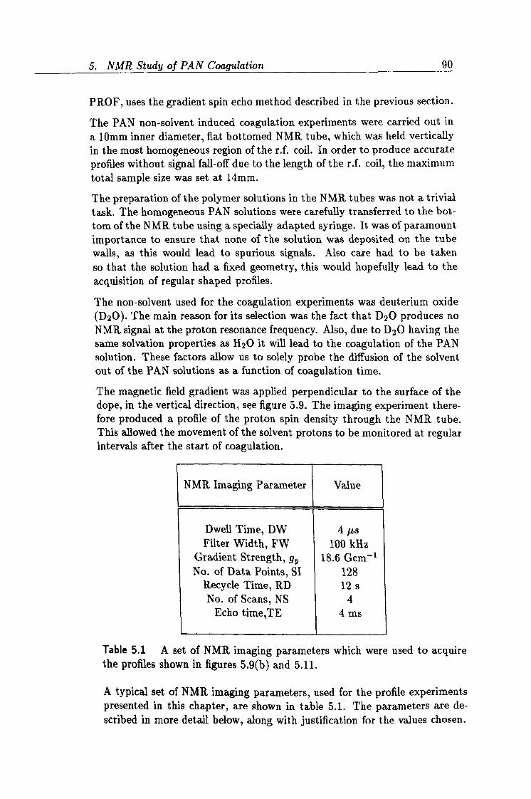
5. NMR Study of PAN Coagulation 90
PROF, uses the gradient spin echo method described in the previous section.
The PAN non-solvent induced coagulation experiments were carried out in
a 10mm inner diameter, flat bottomed NMR tube, which was held vertically in the most homogeneous region of the r. f. coil. In order to produce accurate profiles without signal fall-off due to the length of the r. f. coil, the maximum total sample size was set at 14mm.
The preparation of the polymer solutions in the NMR tubes was not a trivial task. The homogeneous PAN solutions were carefully transferred to the bot- tom of the NMR tube using a specially adapted syringe. It was of paramount importance to ensure that none of the solution was deposited on the tube walls, as this would lead to spurious signals. Also care had to be taken so that the solution had a fixed geometry, this would hopefully lead to the acquisition of regular shaped profiles.
The non-solvent used for the coagulation experiments was deuterium oxide (D20). The main reason for its selection was the fact that D20 produces no NMR signal at the proton resonance frequency. Also, due to D20 having the same solvation properties as H2O it will lead to the coagulation of the PAN solution. These factors allow us to solely probe the diffusion of the solvent out of the PAN solutions as a function of coagulation time.
The magnetic field gradient was applied perpendicular to the surface of the dope, in the vertical direction, see figure 5.9. The imaging experiment there- fore produced a profile of the proton spin density through the NMR tube. This allowed the movement of the solvent protons to be monitored at regular intervals after the start of coagulation.
NMR Imaging Parameter Value
Dwell Time, DW 4 its Filter Width, FW 100 kHz
Gradient Strength, gy 18.6 Gcm-1 No. of Data Points, SI 128
Recycle Time, RD 12 s No. of Scans, NS 4
Echo time, TE 4 ms
Table 5.1 A set of NMR imaging parameters which were used to acquire the profiles shown in figures 5.9(b) and 5.11.
A typical set of NMR imaging parameters, used for the profile experiments presented in this chapter, are shown in table 5.1. The parameters are de- scribed in more detail below, along with justification for the values chosen.
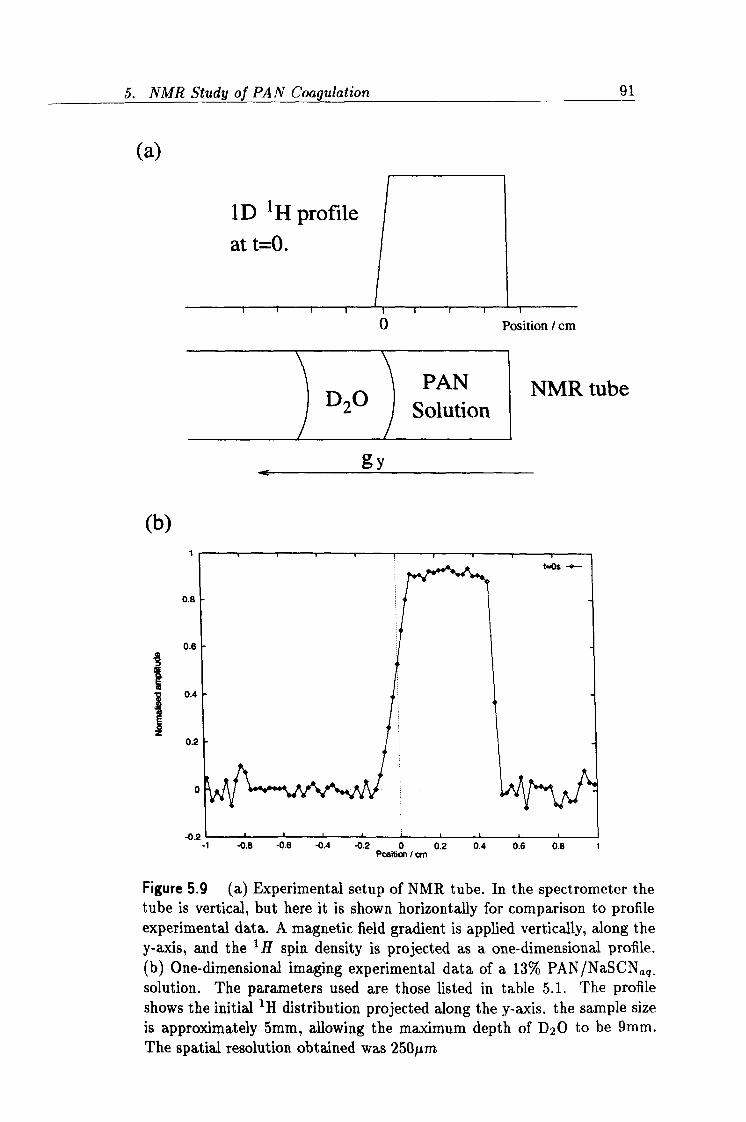
5. NMR Study of PAN Coagulation 91
(a)
PAN NMR tube D20 Solution
gy me
(b)
t-Os -o-
0.6
0.4
-0. s
0.8
0.2
1 -0.8 -0.6 -0.4 -0.2 0 0.2 0.4 0.6 0.8 Potion / cm
Figure 5.9 (a) Experimental setup of NMR tube. In the spectrometer the tube is vertical, but here it is shown horizontally for comparison to profile experimental data. A magnetic field gradient is applied vertically, along the y-axis, and the 'H spin density is projected as a one-dimensional profile. (b) One-dimensional imaging experimental data of a 13% PAN/NaSCN,, q. solution. The parameters used are those listed in table 5.1. The profile shows the initial 1H distribution projected along the y-axis. the sample size is approximately 5mm, allowing the maximum depth of D20 to be 9mm. The spatial resolution obtained was 250µm
0 Position / cm
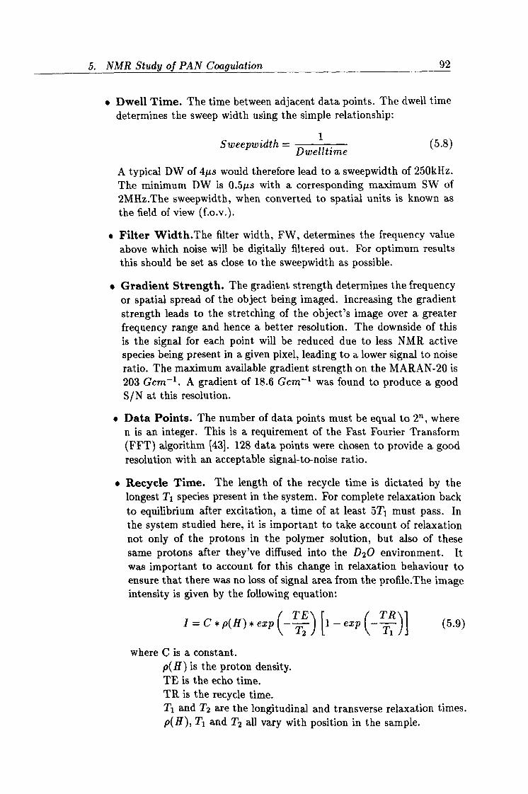
5. NMR Study of PAN Coagulation 92
" Dwell Time. The time between adjacent data points. The dwell time determines the sweep width using the simple relationship:
Sweepwidth =1 (5.8) Dwelltime
A typical DW of 4µs would therefore lead to a sweepwidth of 250kHz. The minimum DW is 0.5µs with a corresponding maximum SW of 2MHz. The sweepwidth, when converted to spatial units is known as the field of view (f. o. v. ).
" Filter Width. The filter width, FW, determines the frequency value above which noise will be digitally filtered out. For optimum results this should be set as close to the sweepwidth as possible.
" Gradient Strength. The gradient strength determines the frequency
or spatial spread of the object being imaged. Increasing the gradient strength leads to the stretching of the object's image over a greater frequency range and hence a better resolution. The downside of this is the signal for each point will be reduced due to less NMR active species being present in a given pixel, leading to a lower signal to noise ratio. The maximum available gradient strength on the MARAN-20 is 203 Gem-. A gradient of 18.6 Gcm-1 was found to produce a good S/N at this resolution.
" Data Points. The number of data points must be equal to 2''s, where n is an integer. This is a requirement of the Fast Fourier Transform (FFT) algorithm [43]. 128 data points were chosen to provide a good resolution with an acceptable signal-to-noise ratio.
" Recycle Time. The length of the recycle time is dictated by the longest Tl species present in the system. For complete relaxation back to equilibrium after excitation, a time of at least 5Ti must pass. In the system studied here, it is important to take account of relaxation not only of the protons in the polymer solution, but also of these same protons after they've diffused into the D20 environment. It was important to account for this change in relaxation behaviour to ensure that there was no loss of signal area from the profile. The image intensity is given by the following equation:
I =C*p(H)*exp( E)
L1 - exp(_TR)j (5.9)
where C is a constant. p(H) is the proton density. TE is the echo time. TR is the recycle time. Ti and T2 are the longitudinal and transverse relaxation times. p(H), Ti and T2 all vary with position in the sample.
5. NMR Study of PAN Coagulation 93
To enable quantitative analysis of the profiles the recycle time must be set to a sufficient length. This was found to be 12s for the system PAN/NaSCNaq. /D20.
" Number of Scans. Increasing the number of scans obviously in- creases the signal to noise ratio, and scales approximately as VN -S. The main limitation placed on the number of scans for this system is the transient nature of the coagulation experiment. From scan to scan the protons in the system will have diffused and therefore the profile will be an average over the number of scans. In the cases presented here for four scans the experiment time was NS * RD = 48s. This seemed an acceptable time for an experiment which took many hours to reach equilibrium.
" Echo time. The echo time is the time between the initial excitation and the centre of the spin-echo. Using equation 5.9, it can be seen that the duration of the echo time, TE, is dictated by the fastest T2 species present. For the system studied here, these are the protons associated with the polyacrylonitrile molecule. From section 3.6 we know for a 13% PAN/NaSCN,,, q. solution, at 30°C, that T2 = llms for the PAN protons. Limitations are placed on the duration of the echo time by the gradient duration and the properties of the gradient coil. Rapid gradient pulse switching is desirable to minimise rise and fall times, and the effects of eddy currents must be taken account of when setting the echo time duration.
Resolution
An intrinsic requirement of the imaging process is that the limit of resolution will occur roughly when the width of the resonance line is comparable to the frequency separation of points in the imaging experiment. The linewidth of the proton resonance is 1kHz, therefore &w > 1kHz.
The relatively low field strength of the MARAN-20 prevented the use of high gradient strengths for the imaging experiment. The spatial resolution obtained using the parameters listed in table 5.1 can be obtained using the following expression:
Ax = AG
(5.10)
where Ox is the spatial resolution. Ow is the frequency resolution, which is obtained from the dwell time. y= 4257 HzG-1, the magnetogyric ratio in the required units. G is the strength of the magnetic field gradient, units Gcm-1.
The spatial resolution obtained using these parameters was therefore 250 µm.
5. NMR Study of PAN Coagulation 94
5.4 Results
The raw data from the one-dimensional, spin-echo, imaging experiment was subjected to post-acquisition processing so that it could be presented in a standard format and to enable modelling of the non-solvent diffusion process. The raw data contains the real and imaginary signal of the spin-echo and needs to undergo a series of steps before the proton density profile in spatial units can be presented. The processing was carried out using the commercial software package IDL [101].
The following processing steps were carried out:
1. The first step is to Fourier transform the raw data using the FFT method [43].
2. The second step is to shift the data so that the profile is in the centre of the f. o. v.
3. The third step is to rephase the raw data so that the maximum profile signal is located in the real channel.
4. The fourth step involves normalising the profiles, taking the profile at time t=0 as the reference.
A set of experimental data for the D20 induced coagulation of a 13% (by wt. ) PAN/NaSCN,,, q. solution is shown in figure 5.10. The spatial distributions of the solvent are shown as one-dimensional profiles and these develop with coagulation time. The profiles were collected every minute and each fifth profile is presented here. A series of profiles from the same data-set are shown in figure 5.11, this time on one set of axes. The development of the profiles can be seen more clearly here. To avoid confusing overlap of the profiles only every tenth data-set is plotted.
There are a few important features of the profiles to note at this juncture:
" The PAN solution initially occupies the spatial region from x=0 to x=5mm. The D20 occupies the region from x=-5mm to x=0. The interface is therefore at x=0.
" The initial profile at t=O is not rectangular in shape but has a slope at the PAN solution/D20 interface, see figure 5.9(b). This can be attributed to the shape of the meniscus associated with the polymer solution.
" There appears to be a spatial position where each profile crosses with approximately the same amplitude. In spectroscopy this is often called an isobestic point.
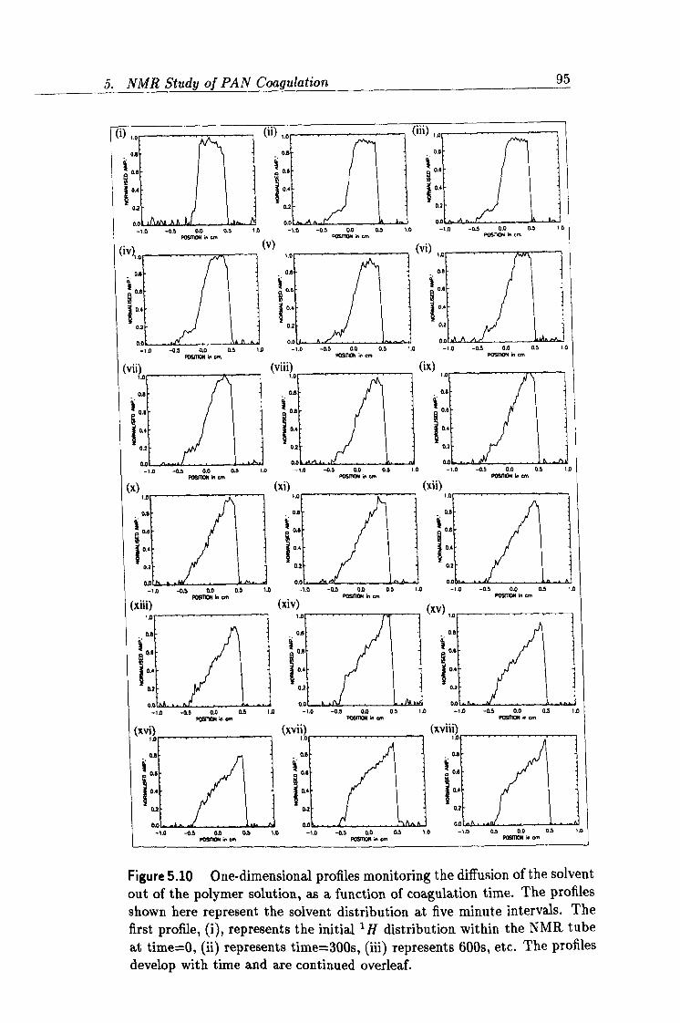
5. NMR Study of PAN Coagulation 95
6.6 Ob O. e
0.6
ý 0.6
ý 0.6
0.1 0.4 0.1
OS 0.2 0.2
0.0 -1.0 -0.5 0.0 0.5
03 1.0 -1.0 -0.5 0.0 0.5
POSITION i m
0.0 1.0 -1.0 -0.5 0.0 0.5 1.0
POSITION in pn POSITION In Nn nc ()
vl\/
0.6 0.8 0. e
0.6 $$$
ýq0.6 ý 0.6
OA 3 O. i O. f
0.2 0.2 0.2
0.0 -0.5 0.0 0.5
A. 0. p 1.0 -1.0 -0.5 0.0 0.5
0.0 1.0 -1.0 -0.5 0.0 03 1,0
POSITION in an POSITION 1. an P09ngn in em
(vii) (viii) (ix) 0 1.0 1.0
0. a DA 0.8
0.6
ý 0.8
ý 0.6
0.4 0.4 OA
p3 OS OS
0.0 OA 0.0
-1A -0.5 0.0 0.5 POSITION in em
1.0 -1.0 -0b 0.0 0.5 POSTION N em
I. 0 -1.0 -0.5 0.0 0.5 1A POSITION in em
(x) (xi) (xii) A LO 7A
0,6 03 03 1
0.6
% 0.6 .6
%
10.4
O. a A
f
0.2 0.. OS
0.0 0.0 OA
-1.0 -0.5 0.0 Ob 1.0 -1.0 -0.5 010 OA 1.0 -1.0 -0.5 0.0 0.5 1.0
(X111} POSITION 1. cm POSITION 0, em (XIV)
POSITION in em
(XV) p to 1
p6 O. e
E /
1.0 5 POSITION 51 an POSTION in pn POSITION in an
(xvi) (xvii) (xviii)
p6 Ob 0.6
0,6
ý
0.6
ý
0.6
0.4 0.1 0.4
I
OS 2
!
0.2
0.0
-0 -0b U 0.5 0.0
O. O 1.0 -1.0 a0 A
-1.0 -0.5 0.0 0.5 .0 POS TI N in an P05105 in cm POSITION in e.
Figure 5.10 One-dimensional profiles monitoring the diffusion of the solvent out of the polymer solution, as a function of coagulation time. The profiles shown here represent the solvent distribution at five minute intervals. The first profile, (i), represents the initial 1H distribution within the NMR tube at time=0, (ii) represents time=300s, (iii) represents 600s, etc. The profiles develop with time and are continued overleaf.
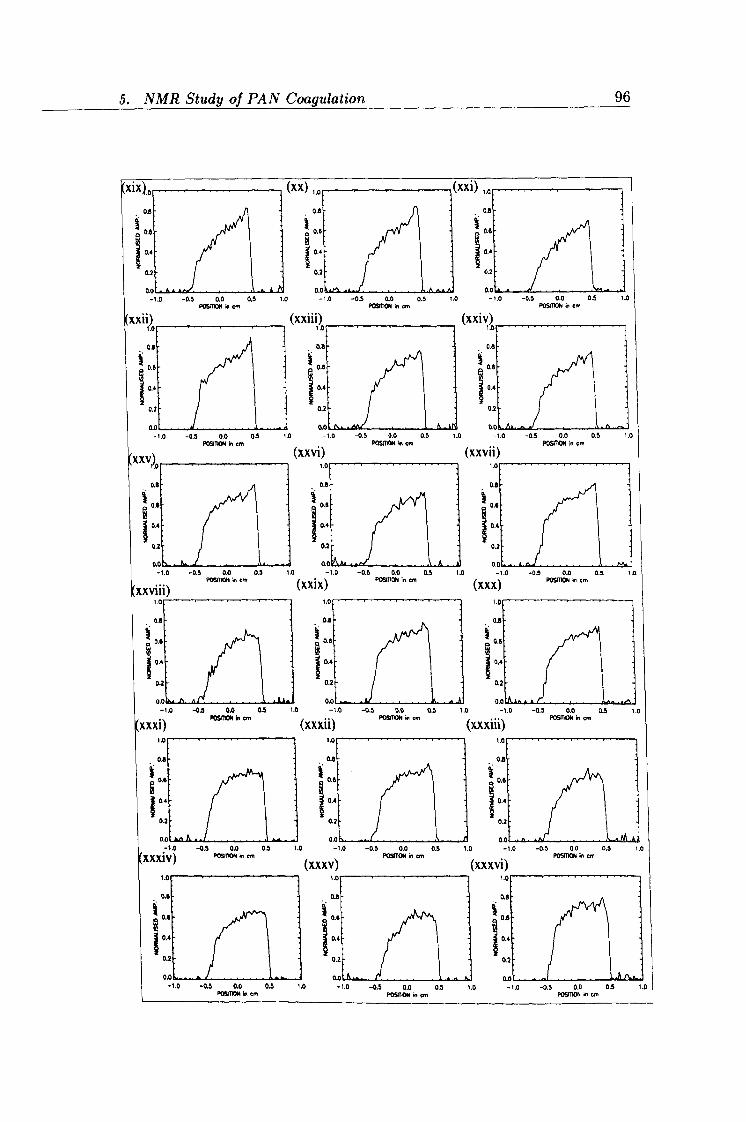
5. NMR Study of PAN Coagulation 96
ýi
(xx)
0,6 ö 0.6
0.4 0.4
0.2 0.2
0.0 0.0 , . -7 -L 1.0 -0.5 0.0 0,5 110 -1.0 -0.5 0.0 0.5 1.0
POSMON in cm POSrtpN h, an
0.2
0.0 1 -0.5 0.0 0.5 1.0
P i, -
-1.0 -0.5 0.0 Ob 1.0 -1.0 -0.5 0.0 0.5 1.0 -1.0 -0.5 0.0 0.5 1.0
1
POSTION in cm (xxvi) POSITION 1n cm
(xxvii) POSITION In cm
i i 7 -1.0 -0.5 0.0 QS 1.0 -1.0 -0.5 0.0 0.5 1.0
(xxix) POSMON in an (xxx) POSR 0.
in tm D -0.5 0.0 0. D
` posmoN In cm
i
DA r
ý. o
o. e
0 0.6
O. i H I "1.0 -0.5 0.0 0.5 110 -1.. -0.5 0.0 0.5 1.0 -1.0 -0.5 0.0 0.5 1.0 POSmON M em (xxxii) PO ON M (xxxiii) POSMON in m
I 1.0
oa
0.6
0.4 D.. F
"1.0 -0.5 0.0 0.5 1.0 -1.0 -0.5 0.0 0.5 1.0 -1.0 -0.5 0.0 0.5 1.0 V\ POSITION in em
(XXXV) POSITION in cm
(xxxvi) POSITION in an
/
ýi ý i. o
o. e
o. 6 3
o. a
-0.5 0.0 0.5 1.0 -1.0 -0.5 0.0 0.5 1.0 -1.0 -0.5 0.0 0.5 1.0 POSITION N, POSf11ON 1n cm P05RION in an
(xxi)
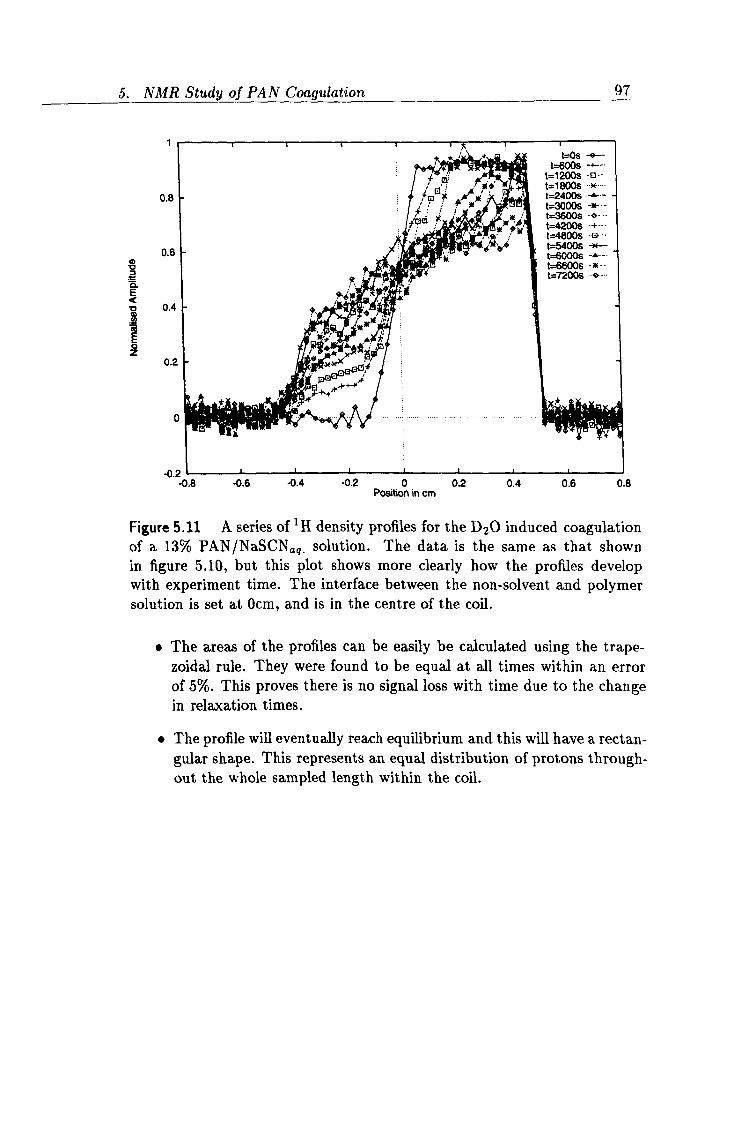
5. NMR Study of PAN Coagulation 97
0.8
0.6 4) 10 Q. E
0.4
02
ý:
k r t=0s -ý- t--600s -+-- t=1200s -ß--
` q ö t=1800s . -x. -- t=24008 -- t=30006 -*- - t
tpa x ýIxým. t=3800s -o--- t=4200s -+--- t=48006 -a -
d'"tyy4 t=5400s yý ° t=60006
il. " t--6600s -* -- @ ,
rr t_7200s . o.. _ ~
A"ýyt A" d
" rrf i: i
fý g ýk#r
ýý 4
0.8 -0.6 -0.4 -0.2 0 0.2 0.4 0.6 0.8 Position in cm
Figure 5.11 A series of 1H density profiles for the D20 induced coagulation of a 13% PAN/Na5CNa, 9. solution. The data is the same as that shown in figure 5.10, but this plot shows more clearly how the profiles develop with experiment time. The interface between the non-solvent and polymer solution is set at 0cm, and is in the centre of the coil.
The areas of the profiles can be easily be calculated using the trape- zoidal rule. They were found to be equal at all times within an error of 5%. This proves there is no signal loss with time due to the change in relaxation times.
" The profile will eventually reach equilibrium and this will have a rectan- gular shape. This represents an equal distribution of protons through- out the whole sampled length within the coil.
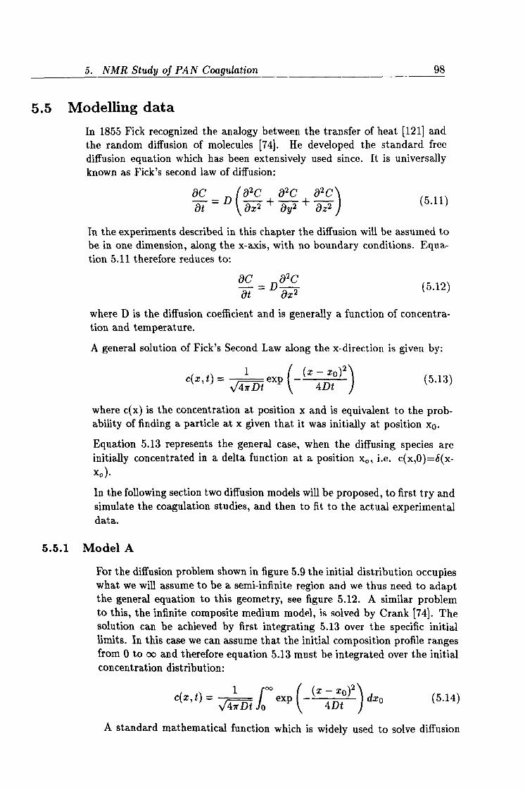
5. NMR Study of PAN Coagulation 98
5.5 Modelling data In 1855 Fick recognized the analogy between the transfer of heat [121] and the random diffusion of molecules [74]. He developed the standard free diffusion equation which has been extensively used since. It is universally known as Fick's second law of diffusion:
ac a2c a2c a2c 1
at =D ax2 +a2+
az2 5.11 J
In the experiments described in this chapter the diffusion will be assumed to be in one dimension, along the x-axis, with no boundary conditions. Equa- tion 5.11 therefore reduces to:
2 Ft
axe (5.12) D
where D is the diffusion coefficient and is generally a function of concentra- tion and temperature.
A general solution of Fick's Second Law along the x-direction is given by:
c(x, t) =1 exp (5.13) 4 irDt 4Dt
where c(x) is the concentration at position x and is equivalent to the prob- ability of finding a particle at x given that it was initially at position xo. Equation 5.13 represents the general case, when the diffusing species are initially concentrated in a delta function at a position x0, i. e. c(x, 0)=b(x- xo).
In the following section two diffusion models will be proposed, to first try and simulate the coagulation studies, and then to fit to the actual experimental data.
5.5.1 Model A
For the diffusion problem shown in figure 5.9 the initial distribution occupies what we will assume to be a semi-infinite region and we thus need to adapt the general equation to this geometry, see figure 5.12. A similar problem to this, the infinite composite medium model, is solved by Crank [74]. The solution can be achieved by first integrating 5.13 over the specific initial limits. In this case we can assume that the initial composition profile ranges from 0 to oo and therefore equation 5.13 must be integrated over the initial concentration distribution:
C(x't) 1 °°
exp (x - xo)2 dxo (5.14)
47 Dt lo
4Dt
A standard mathematical function which is widely used to solve diffusion
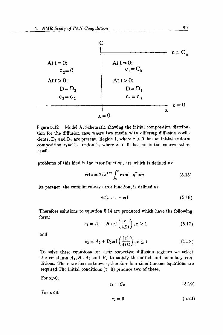
5. NMR Study of PAN Coagulation 99
Att=0: c2=0
Att>0: D=D2 C2=C2
c
Att=O: cl=Co
Att>0: D=D1 cI=c. 1
x x=0
C=Co
C=O
Figure 5.12 Model A. Schematic showing the initial composition distribu- tion for the diffusion case where two media with differing diffusion coeffi- cients, D1 and D2 are present. Region 1, where x>0, has an initial uniform composition c1=Co. region 2, where x<0, has an initial concentration c2=0.
problems of this kind is the error function, erf, which is defined as:
erfz = 2/ir1/2 jZ exp(-r72)drý (5.15)
Its partner, the complimentary error function, is defined as:
erfc =1- erf (5.16)
Therefore solutions to equation 5.14 are produced which have the following form:
and
c1 = Ai + Bierf 4Dt 'x>1
(5.17)
c2=A2+B2erf( , ),
x<1 (5.18)
To solve these equations for their respective diffusion regimes we select the constants Ai, Bi, A2 and B2 to satisfy the initial and boundary con- ditions. There are four unknowns, therefore four simultaneous equations are required. The initial conditions (t=0) produce two of these:
For x>O, Cl = Co (5.19)
For x<O, C2 =0 (5.20)
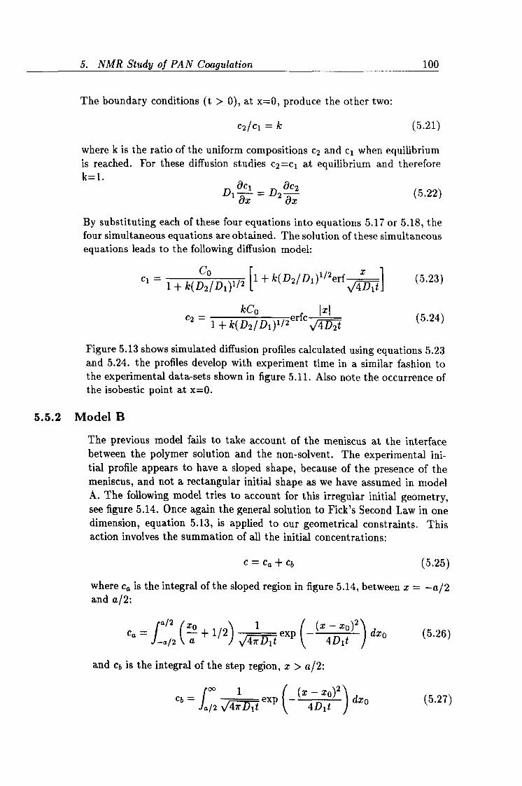
5. NMR Study of PAN Coagulation 100
The boundary conditions (t > 0), at x=0, produce the other two:
C2/c1 =k (5.21)
where k is the ratio of the uniform compositions c2 and cl when equilibrium is reached. For these diffusion studies c2=c1 at equilibrium and therefore k=1.
(5.22) Dl x
D2 ax 8
By substituting each of these four equations into equations 5.17 or 5.18, the four simultaneous equations are obtained. The solution of these simultaneous equations leads to the following diffusion model:
1+1 (5.23) Cl = D2/ 1ý2 I1+ k(D2/Di)1/2erf x
( /Dl) ` 4Dlt 1
C2 =D °D / erfc 4lx' Dt
(5.24) 1+ k( 2l1)1 2
Figure 5.13 shows simulated diffusion profiles calculated using equations 5.23 and 5.24. the profiles develop with experiment time in a similar fashion to the experimental data-sets shown in figure 5.11. Also note the occurrence of the isobestic point at x=0.
5.5.2 Model B
The previous model fails to take account of the meniscus at the interface between the polymer solution and the non-solvent. The experimental ini- tial profile appears to have a sloped shape, because of the presence of the meniscus, and not a rectangular initial shape as we have assumed in model A. The following model tries to account for this irregular initial geometry, see figure 5.14. Once again the general solution to Fick's Second Law in one dimension, equation 5.13, is applied to our geometrical constraints. This action involves the summation of all the initial concentrations:
_ Ca + Cb (5.25
where ca is the integral of the sloped region in figure 5.14, between x= -a/2 and a/2:
Ca J-alj (
ao +1/2)
47rDit exp -(x4Dit)2 dxo (5.26)
and eb is the integral of the step region, x> a/2:
Cb a2 41 t eXp
(X -t )2 dx° (5.27)
J/ i
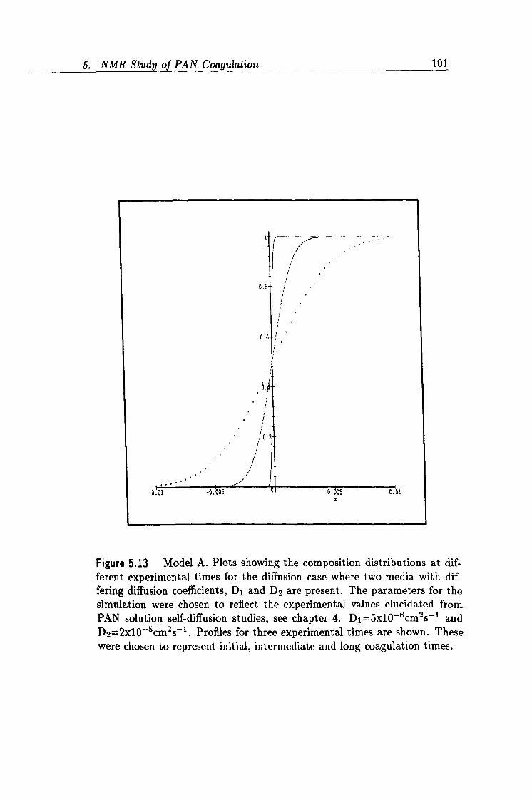
5. NMR Study of PAN Coagulation 101
Figure 5.13 Model A. Plots showing the composition distributions at dif- ferent experimental times for the diffusion case where two media with dif- fering diffusion coefficients, D1 and D2 are present. The parameters for the simulation were chosen to reflect the experimental values elucidated from PAN solution self-diffusion studies, see chapter 4. D1=5x10⁻⁶cm2s-1 and D2=2x10⁻⁵cm2s-1. Profiles for three experimental times are shown. These were chosen to represent initial, intermediate and long coagulation times.
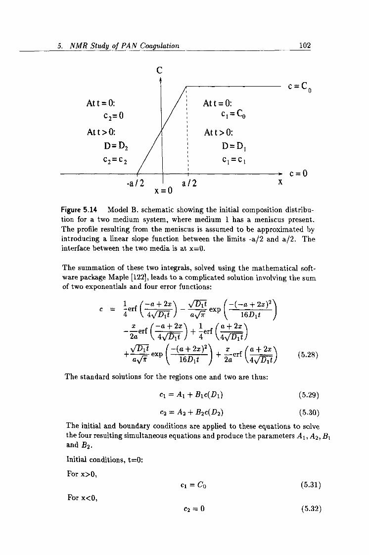
5. NMR Study of PAN Coagulation 102
c
Att=0: c2=
Att>0: D= D2
c2=c2
-a/2 a/2 x=0
c=Co Att=0:
ci=Co
Att>0: D=D1 c1=c1
c=0 x
Figure 5.14 Model B. schematic showing the initial composition distribu- tion for a two medium system, where medium 1 has a meniscus present. The profile resulting from the meniscus is assumed to be approximated by introducing a linear slope function between the limits -a/2 and a/2. The interface between the two media is at x=0.
The summation of these two integrals, solved using the mathematical soft- ware package Maple [1221, leads to a complicated solution involving the sum of two exponentials and four error functions:
c=1 erf -a + 2x Dlt eX -(-a + 2x)2
4 (4
Dlt )
aý P 16D1t
x (_a+2x\ 1 a+2x - 2aerf 4 Dlt
14erf (4 Dlt)
Dlt -(a + 2x)2 xa+ 2x ) +
aý exp 16D1t + 2aerf
(4 Dit)
(5.2$
The standard solutions for the regions one and two are thus:
cl = Ai + Bic(D1) (5.29)
c2 = A2 + B2c(D2) (5.30)
The initial and boundary conditions are applied to these equations to solve the four resulting simultaneous equations and produce the parameters A,,, A2, Bl and B2.
Initial conditions, t=0:
For x>O, ci=Co (5.31)
For x<O, c2 =0 (5.32)
5. NMR Study of PAN Coagulation 103
The boundary conditions (t > 0) are, at x=0:
C2 = Cl (5.33)
D1 Oac,
&C2
x D2
äx (5.34)
The following relationships result:
2COD2erf (° 2t) B2 = (5.35)
Dierf (4 lt)
+ D2erf (4VD)
A2 = B2 (5.36)
Al = A2 (5.37)
Bl = 2Co - B2 (5.38)
These parameters can be substituted back into equations 5.29 and 5.30 to obtain the diffusion equations describing the region one:
COD2erf (_a 4 2t) cl (x, t) =
Dlerf (-47'r lt)
+ D2erf (4 a Ztý
2C0D2erf (4 a 2t) ý- c (5.39)
+ D2erf ý4 ° Zt
Dlerf (4vi)
where c is defined as in equation 5.28. For region two:
COD2erf ('_) C2(ist) z
l Dererf(4 alt)-}D2erf14 a2tý 775- D2erf (a)
4 +2Co 1-2c (5.40) Dlerf (4 °
lt) + D2erf ())
The shape of these functions can be visualised by substituting model param- eters into these equations, and plotting the resulting curves, see figure 5.15.
5.5.3 Fitting data to the models The experimental data was fitted to the diffusion model using procedures written in the IDL development package [101]. The POWELL optimization procedure [63] was used to minimise the square of the differences between the fit and the data. The method uses successive line minimizations without the need for explicit calculation of the function's gradient.
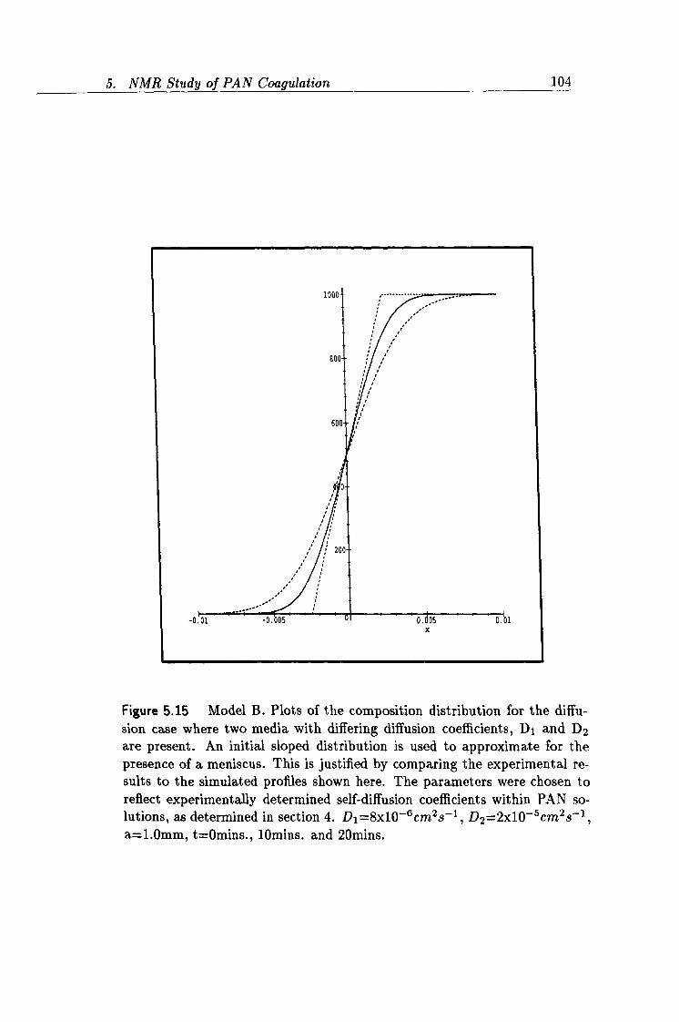
5. NMR Study of PAN Coagulation 104
Figure 5.15 Model B. Plots of the composition distribution for the diffu- sion case where two media with differing diffusion coefficients, Di and D2 are present. An initial sloped distribution is used to approximate for the presence of a meniscus. This is justified by comparing the experimental re- sults to the simulated profiles shown here. The parameters were chosen to reflect experimentally determined self-diffusion coefficients within PAN so- lutions, as determined in section 4. D1=8x10⁻⁶cm2s-1, D2=2x10⁻⁵cm2s-1, a=1. Omm, t=Omins., 10mins. and 20mins.
5. NMR Study of PAN Coagulation 105
We now have two models which can be used to attempt to fit the coagulation data. Model B is an enhanced version of model A to take account of the irregular initial profile shape caused by the meniscus. If comparison is made between the simulated data, shown in figure 5.15, and the experimental data, shown earlier in figure 5.11, it can be seen that there is close relation between the two data-sets. The fitting procedures also return a parameter fmin, which is the sum of the square of the differences between the data and the fit. This value was consistently lower for model B than for model A. Due to this selection criterion model B was chosen to fit the coagulation data and produce quantitative diffusion data.
The two functions 5.39 and 5.40 were simultaneously fitted to the experimen- tal data. Computed values for the variables D1, D2 and Co were returned. It was necessary to predict the cross-over point between regime one (with diffusion coefficient D1) and regime two (with diffusion coefficient D2). This was chosen to be at a normalised profile amplitude of 0.5 on the initial profile (time=Omin. ). It is reasonable to select this position as it is roughly at the mid-point of the meniscus and therefore is a good approximation for where the interface between the PAN solution and the D20 lies.
The spatial range over which the concentration is fitted, spans from the bottom of the NMR tube to either the limit of the D20 or to the lower limit of the f. o. v. As the spatial area between these two limits is composed of random background noise, then the fits should be identical and not dependent on which limit is chosen. This was found to be the case and therefore the lower limit of the f. o. v. was chosen and a total of approximately 90 points were fitted.
5.5.4 Validity of models Model B was selected to fit the experimental data as the model profiles were more comparable to the coagulation data. Figure 5.16 shows the initial ex- perimental profile before the coagulation has commenced. The fit agrees well with the experimental data-set providing evidence that the linear gra- dient function is a good approximation for modelling the projection of the meniscus. The profile initially is spanned by approximately twenty points and this proves adequate for fitting the three parameters, D1, D2 and Co.
Figures 5.17,5.18 and 5.19 present further fits to the experimental data using diffusion model B. Each one shows good agreement between experimental data and the corresponding fit.
Table 5.2 shows the dependence of the diffusion coefficients D1 and D2 on the coagulation time. The data is presented for every fifth profile, i. e. at five minute intervals, up to a coagulation time of seventy minutes. The same data-set is plotted in figure 5.20 to display the variations more clearly. From the figure we can see that after an initial period of 15-20 minutes the dif- fusion coefficients begin to follow regular trends. D1, which represents the
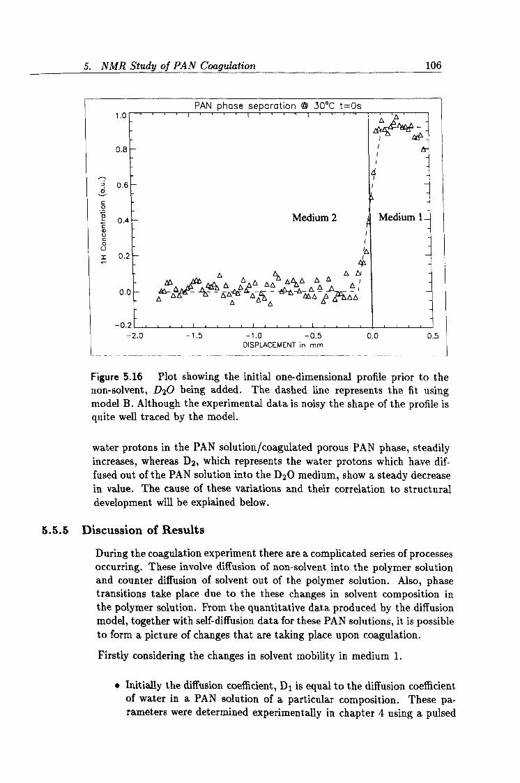
5. NMR Study of PAN Coagulation 106
1.0
0.8
0.6 ö
C 0
0.4 C 0) U C O
U
= o. ý
0. f
-o.
PAN phase separation ® 30°C t=Os
Figure 5.16 Plot showing the initial one-dimensional profile prior to the non-solvent, D20 being added. The dashed line represents the fit using model B. Although the experimental data is noisy the shape of the profile is quite well traced by the model.
water protons in the PAN solution/coagulated porous PAN phase, steadily increases, whereas D2, which represents the water protons which have dif- fused out of the PAN solution into the D20 medium, show a steady decrease in value. The cause of these variations and their correlation to structural development will be explained below.
5.5.5 Discussion of Results
During the coagulation experiment there are a complicated series of processes occurring. These involve diffusion of non-solvent into the polymer solution and counter diffusion of solvent out of the polymer solution. Also, phase transitions take place due to the these changes in solvent composition in the polymer solution. From the quantitative data produced by the diffusion model, together with self-diffusion data for these PAN solutions, it is possible to form a picture of changes that are taking place upon coagulation.
Firstly considering the changes in solvent mobility in medium 1.
" Initially the diffusion coefficient, D1 is equal to the diffusion coefficient of water in a PAN solution of a particular composition. These pa- rameters were determined experimentally in chapter 4 using a pulsed
-2.0 -1.5 -1.0 -0.5 0.0 0.5 DISPLACEMENT in mm
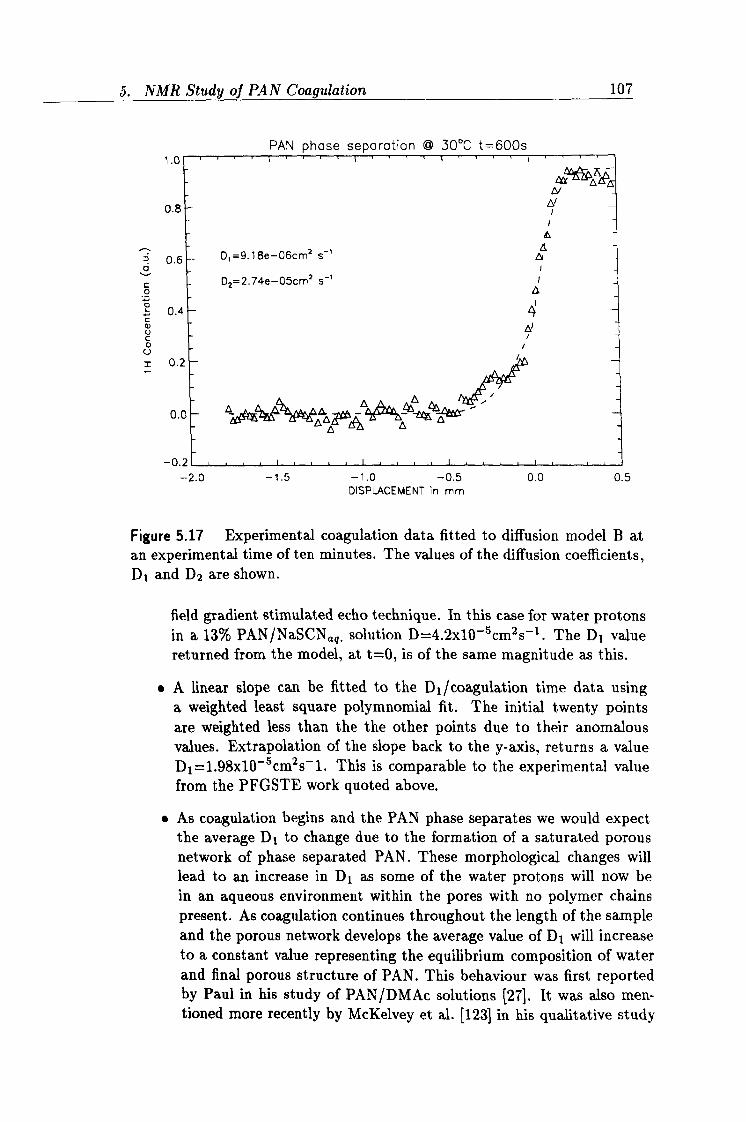
5. NMR Study of PAN Coagulation 107
1.0
0.8
0.6 O
C 0
0.4 Q) U C O
U
0. (
-0.
PAN phase separation @ 30°C t=600s
4U N
D, =9.18e-06cm2 s-'
D2=2.74e-05cm2 s-' 4 4'
4yg'
p üý
-2.0 -1.5 -1.0 -0.5 0.0 0.5 DISPLACEMENT in mm
Figure 5.17 Experimental coagulation data fitted to diffusion model B at an experimental time of ten minutes. The values of the diffusion coefficients, D1 and D2 are shown.
field gradient stimulated echo technique. In this case for water protons in a 13% PAN/NaSCN,, q. solution D=4.2x10⁻⁵cm2s-1. The D1 value returned from the model, at t=0, is of the same magnitude as this.
"A linear slope can be fitted to the Di/coagulation time data using a weighted least square polymnomial fit. The initial twenty points are weighted less than the the other points due to their anomalous values. Extrapolation of the slope back to the y-axis, returns a value D1=1.98x10⁻⁵cm2s-1. This is comparable to the experimental value from the PFGSTE work quoted above.
" As coagulation begins and the PAN phase separates we would expect the average D1 to change due to the formation of a saturated porous network of phase separated PAN. These morphological changes will lead to an increase in D1 as some of the water protons will now be in an aqueous environment within the pores with no polymer chains present. As coagulation continues throughout the length of the sample and the porous network develops the average value of Di will increase to a constant value representing the equilibrium composition of water and final porous structure of PAN. This behaviour was first reported by Paul in his study of PAN/DMAc solutions [27]. It was also men- tioned more recently by McKelvey et al. [123] in his qualitative study
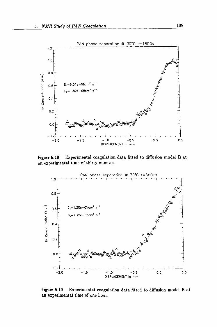
5. NMR Study of PAN Coagulation 108
-. - ,,. - --0- .. ---
1.2
1.0
rrAiv Ni iuac Z)cNuI ULIUI I ,wL L- I uvva
0.8
ö 0. E ö
0 U 2
0.1
0.1
-0.
0, =9.01 e-06cmZ s-'
D2=1.82e-05cm2 s-'
I 4Qd''°
°
-2.0 -1.5 -1.0 -0.5 0.0 0.5 DISPLACEMENT in mm
Figure 5.18 Experimental coagulation data fitted to diffusion model B at an experimental time of thirty minutes.
PAN phase separation @ 30°C t=3600s 1.0
0.8
0.6
C O
O a"4
c d V C O
U
r 0.1
0.1
-0.21 III -2.0 -1.5 -1.0 -0.5 0.0 0.5
DISPLACEMENT in mm
Figure 5.19 Experimental coagulation data fitted to diffusion model B at an experimental time of one hour.
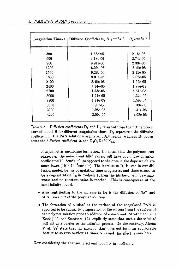
5. NMR Study of PAN Coagulation 109
Coagulation Time/s Diffusion Coefficients, DI/cm 2s-1 D2/cm2s-1
300 1.88e-05 2.16e-05 600 9.18e-06 2.74e-05 900 9.91e-06 2.33e-05 1200 6.99e-06 2.18e-05 1500 9.28e-06 2.1 le-05 1800 9.01e-06 2.02e-05 2100 8.48e-06 1.62e-05 2400 1.14e-05 1.77e-05 2700 1.33e-05 1.61e-05 3000 1.24e-05 1.32e-05 3300 1.71e-05 1.59e-05 3600 1.99e-05 1.39e-05 3900 1.98e-05 1.31e-05 4200 2.09e-05 1.08e-05
Table 5.2 Diffusion coefficients D1 and D2 returned from the fitting proce- dure of model B for different coagulation times. D1 represents the diffusion coefficient in the PAN solution/ coagulated PAN region, whereas D2 repre- sents the diffusion coefficient in the D20/NaSCNaq..
of asymmetric membrane formation. He noted that the polymer-lean phase, i. e. the non-solvent filled pores, will have liquid like diffusion coefficients(10-5cm2s-1), as opposed to the ones in the dope which are much lower (10'7-10-8cm2s-1). The increase in D1 is seen in our dif- fusion model, but as coagulation time progresses, and there ceases to be a concentration Co in medium 1, then the fits become increasingly worse and no constant value is reached. This is consequence of the semi-infinite model.
" Also contributing to the increase in D1 is the diffusion of Na+ and SCN- ions out of the polymer solution.
" The formation of a `skin' at the surface of the coagulated PAN is reported to be caused by evaporation of the solvent from the surface of the polymer solution prior to addition of non-solvent. Strathmann and Kock [119] and Smolders [124] explicitly state that such a dense ̀ skin' will act as a barrier to the diffusion process. On the contrary, Altena et al. [29] state that the nascent `skin' does not form an appreciable barrier to solvent outflow at times > 5s and this effect is seen here.
Now considering the changes in solvent mobility in medium 2:
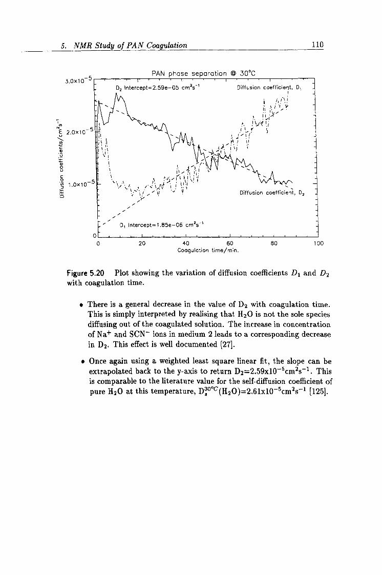
5. NMR Study of PAN Coagulation 110
3.0x10⁻⁵
2.0x10⁻⁵
4) 0 L) C O
_c 1. Ox1O
0
PAN phase separation ® 30°C
Figure 5.20 Plot showing the variation of diffusion coefficients D1 and D2 with coagulation time.
" There is a general decrease in the value of D2 with coagulation time. This is simply interpreted by realising that H2O is not the sole species diffusing out of the coagulated solution. The increase in concentration of Na+ and SCN- ions in medium 2 leads to a corresponding decrease in D2. This effect is well documented (271.
" Once again using a weighted least square linear fit, the slope can be extrapolated back to the y-axis to return D2=2.59x10⁻⁵cm2s-1. This is comparable to the literature value for the self-diffusion coefficient of pure H2O at this temperature, D8°°C(H20)=2.61x10⁻⁵cm2s`1 [125].
0 20 40 60 80 100 Coagulation time/min.
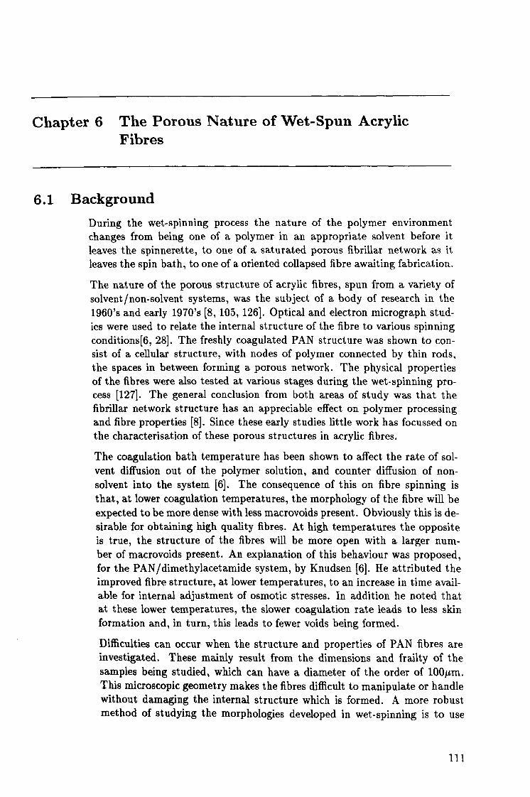
Chapter 6 The Porous Nature of Wet-Spun Acrylic Fibres
6.1 Background During the wet-spinning process the nature of the polymer environment changes from being one of a polymer in an appropriate solvent before it leaves the spinnerette, to one of a saturated porous fibrillar network as it leaves the spin bath, to one of a oriented collapsed fibre awaiting fabrication.
The nature of the porous structure of acrylic fibres, spun from a variety of solvent/non-solvent systems, was the subject of a body of research in the 1960's and early 1970's [8,105,126]. Optical and electron micrograph stud- ies were used to relate the internal structure of the fibre to various spinning conditions[6,28]. The freshly coagulated PAN structure was shown to con- sist of a cellular structure, with nodes of polymer connected by thin rods, the spaces in between forming a porous network. The physical properties of the fibres were also tested at various stages during the wet-spinning pro- cess [127]. The general conclusion from both areas of study was that the fibrillar network structure has an appreciable effect on polymer processing and fibre properties [8]. Since these early studies little work has focussed on the characterisation of these porous structures in acrylic fibres.
The coagulation bath temperature has been shown to affect the rate of sol- vent diffusion out of the polymer solution, and counter diffusion of non- solvent into the system [6]. The consequence of this on fibre spinning is that, at lower coagulation temperatures, the morphology of the fibre will be expected to be more dense with less macrovoids present. Obviously this is de- sirable for obtaining high quality fibres. At high temperatures the opposite is true, the structure of the fibres will be more open with a larger num- ber of macrovoids present. An explanation of this behaviour was proposed, for the PAN/dimethylacetamide system, by Knudsen [6]. He attributed the improved fibre structure, at lower temperatures, to an increase in time avail- able for internal adjustment of osmotic stresses. In addition he noted that at these lower temperatures, the slower coagulation rate leads to less skin formation and, in turn, this leads to fewer voids being formed.
Difficulties can occur when the structure and properties of PAN fibres are investigated. These mainly result from the dimensions and frailty of the samples being studied, which can have a diameter of the order of 100µm. This microscopic geometry makes the fibres difficult to manipulate or handle without damaging the internal structure which is formed. A more robust method of studying the morphologies developed in wet-spinning is to use
111
6. The Porous Nature of Wet-Spun Acrylic Fibres 112
Non-solvent Bath NS S
Polymer Solution
Support
Figure 6.1 Schematic of the membrane immersion precipitation process. The labels NS and S represent diffusion of the non-solvent and solvent re- spectively.
techniques developed in the field of membrane research [128], which involve the casting of thin films. Although there are differences between the detailed aspects of membrane casting and fibre spinning, the most obvious being the static aspect of membrane casting, it has been demonstrated that the two methods produce similar structures [26].
The preparation of so called immersion precipitation membranes utilizes a similar strategy to that employed in the wet-spinning of fibres. The membrane forming polymer, dissolved in a suitable solvent, is cast onto an inert support and then immersed in a non-solvent bath, see figure 6.1. Solvent/non-solvent counter diffusion is allowed to take place, until phase separation of the polymer has occurred. The membrane adopts a porous structure, which at this stage will be filled with an equilibrium composition of solvent and non-solvent. The structure of the membrane depends on the casting parameters in the same way as fibre morphologies are determined by the spinning parameters. The size of the membrane depends on the geometry of the support and the depth of the film which is cast.
It is often desirable in certain membrane applications to form a dense skin at the surface of the membrane [129]. For example in ultra-filtration mem- branes, such a permselective barrier is essential for the separation of species with different transport properties. These membranes which are composed of a dense skin, supported by a more porous network were developed in the early 1960's and are commonly known as asymmetric or anisotropic mem- branes [130]. The advantages of this structure over previously used thin film membranes is that mechanical integrity problems are eliminated. This type of structure has been reported to develop in acrylic fibres under certain
6. The Porous Nature of Wet-Spun Acrylic Fibres 113
conditions and SEM data has confirmed its existence [26].
In this chapter PAN films cast at a range of different coagulation tem- peratures are studied. The transverse relaxation times and self diffusion coefficients of non-solvent water molecules trapped in the porous network have been measured. These experiments produce NMR parameters which can be related to physical structural parameters. Scanning electron mi- croscopy(SEM) data are also be presented, which complement the NMR studies.
6.2 Film Preparation A 13% PAN/NASCNaq. dope was selected for the experiments described in this chapter. The PAN films were prepared using the following method:
" The PAN solution is cast onto a glass plate (Area 26mm x 76mm) to a depth of approximately 5mm. This can be achieved by spreading the viscous dope to the required dimensions using a glass slide.
" The cast dope is immediately immersed in a non-solvent bath con- taining a large volume of water at a well-defined temperature. The coagulation can be observed by the PAN solution becoming turbid or opaque.
" After the coagulation had taken place and the solution reached an equilibrium composition (approximately 30 minutes) the PAN film can be removed from the bath.
" The excess water is removed from the surface of the PAN film by carefully blotting with paper.
" The above steps are then repeated for a series of PAN films at different coagulation temperatures.
The prepared PAN films are used immediately after preparation to minimize the risk of evaporation of the liquid filling the pores and potentially collapse of the internal structure. The NMR characterisation experiments described in the following sections can then be carried out.
6. The Porous Nature of Wet-Spun Acrylic Fibres 114
6.3 NMR Transverse Relaxation Studies
NMR transverse relaxation experiments provide information regarding the mobilities of species within their local environment. In the experiments de-
scribed here the 111 NMR transverse relaxation behaviour of water protons contained in the porous network of PAN films, prepared at various temper- atures, was characterised. The confinement of the solvent in the geometry of the porous structure leads to a change in their relaxation properties. The films were cast at a range of different coagulation temperatures to investi- gate the relationship between T2 and any change in the pore structure of the films. It is known that the mobility of small molecules in a porous network is directly related to the average pore size and the pore size distribution [109]. From the experimental results it is possible to obtain quantitative data for these parameters. Calculations of this kind have been extensively used in the field of porous rocks, which has important applications in the oil indus- try [131], and also in the study of biological cells [132,133].
6.3.1 The Method
The experiments were conducted using the Resonance Instruments MARAN- 20 benchtop NMR spectrometer, as described in section 3.4.2. The pulse sequence used to obtain the relaxation data presented in this section was the Meiboom-Gill modification of the Carr-Purcell method [581. Every second echo was acquired with 2T=500µs and a total number of echoes =1024. The tau dependence of T2 was investigated, but little variation was seen in the region studied.
The preliminary fittings of the T2 relaxation data was carried out using CONTIN. This was used to investigate the number of components present in the decay curves, see section 3.4.3. These fits consistently produced sin- gle exponential fits for the PAN films studied. The final fits were carried out using the package XFIT which produces relaxation times in very close agreement with those obtained using CONTIN (see section 3.4.3). Once the number of components is known, XFIT produces similar relaxation times to CONTIN, the benefit being that it allows more rapid processing of the data.
6.3.2 Results
The T2 relaxation data of non-solvent water protons confined in the porous network of PAN films, cast at a range of temperatures, is presented in ta- ble 6.1. The T2 values quoted represent the mean value of three independent castings of the films. The error is also quoted showing good agreement be- tween experiments.
The general trend shown in table 6.1 shows that there is an increase in T2 relaxation time with elevation of the casting temperature. A variation in T2 can sometimes be interpreted as a change in the mobility of the species being studied. An increase in T2 would therefore mean that the system has become
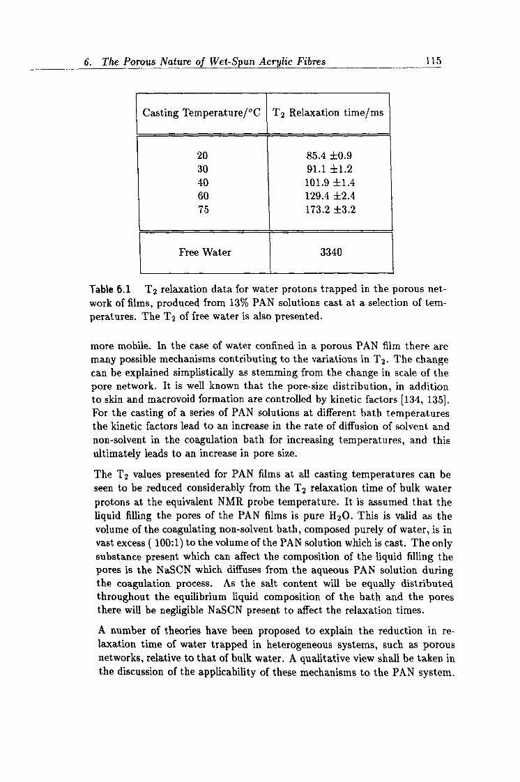
6. The Porous Nature of Wet-Spun Acrylic Fibres 115
Casting Temperature/°C T2 Relaxation time/ms
20 85.4 ±0.9 30 91.1 ±1.2 40 101.9 ±1.4 60 129.4 ±2.4 75 173.2 ±3.2
Free Water 3340
Table 6.1 T2 relaxation data for water protons trapped in the porous net- work of films, produced from 13% PAN solutions cast at a selection of tem- peratures. The T2 of free water is also presented.
more mobile. In the case of water confined in a porous PAN film there are many possible mechanisms contributing to the variations in T2. The change can be explained simplistically as stemming from the change in scale of the pore network. It is well known that the pore-size distribution, in addition to skin and macrovoid formation are controlled by kinetic factors [134,135]. For the casting of a series of PAN solutions at different bath temperatures the kinetic factors lead to an increase in the rate of diffusion of solvent and non-solvent in the coagulation bath for increasing temperatures, and this ultimately leads to an increase in pore size.
The T2 values presented for PAN films at all casting temperatures can be seen to be reduced considerably from the T2 relaxation time of bulk water protons at the equivalent NMR probe temperature. It is assumed that the liquid filling the pores of the PAN films is pure 1120. This is valid as the volume of the coagulating non-solvent bath, composed purely of water, is in vast excess ( 100: 1) to the volume of the PAN solution which is cast. The only substance present which can affect the composition of the liquid filling the pores is the NaSCN which diffuses from the aqueous PAN solution during the coagulation process. As the salt content will be equally distributed throughout the equilibrium liquid composition of the bath and the pores there will be negligible NaSCN present to affect the relaxation times.
A number of theories have been proposed to explain the reduction in re- laxation time of water trapped in heterogeneous systems, such as porous networks, relative to that of bulk water. A qualitative view shall be taken in the discussion of the applicability of these mechanisms to the PAN system.
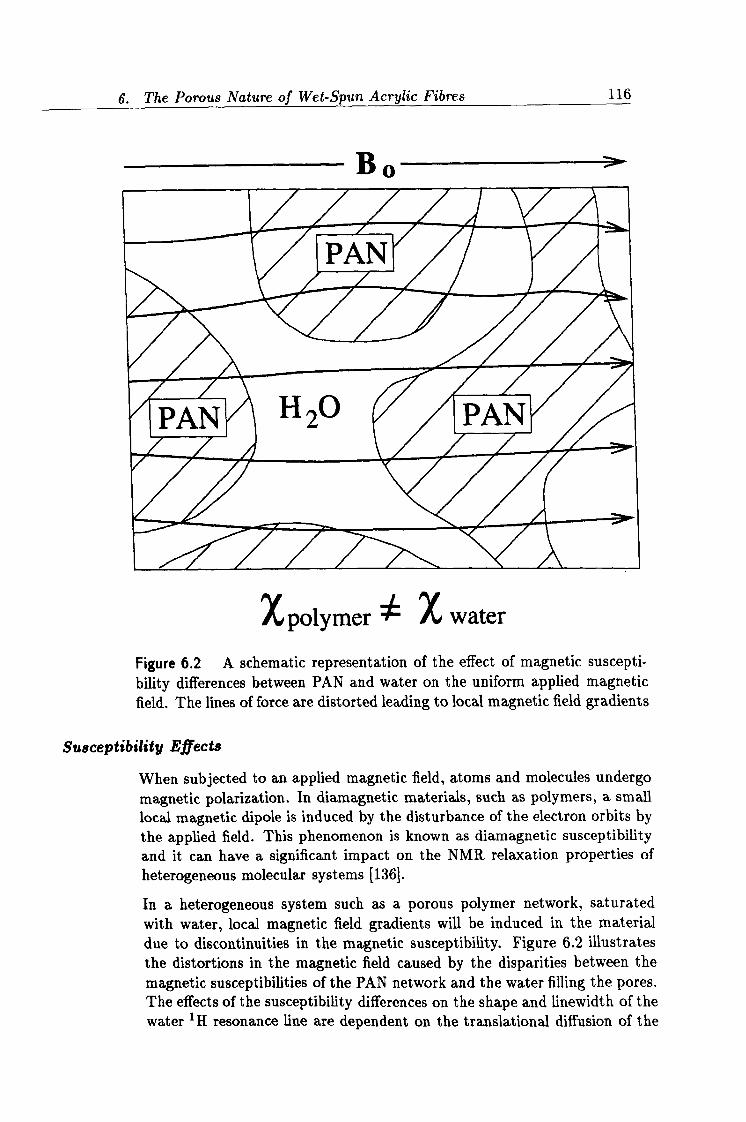
6. The Porous Nature of Wet-Spun Acrylic Fibres 116
/ý polymer iX
water Figure 6.2 A schematic representation of the effect of magnetic suscepti- bility differences between PAN and water on the uniform applied magnetic field. The lines of force are distorted leading to local magnetic field gradients
Susceptibility Effects
When subjected to an applied magnetic field, atoms and molecules undergo magnetic polarization. In diamagnetic materials, such as polymers, a small local magnetic dipole is induced by the disturbance of the electron orbits by the applied field. This phenomenon is known as diamagnetic susceptibility and it can have a significant impact on the NMR relaxation properties of heterogeneous molecular systems [1361.
In a heterogeneous system such as a porous polymer network, saturated with water, local magnetic field gradients will be induced in the material due to discontinuities in the magnetic susceptibility. Figure 6.2 illustrates the distortions in the magnetic field caused by the disparities between the magnetic susceptibilities of the PAN network and the water filling the pores. The effects of the susceptibility differences on the shape and linewidth of the water '11 resonance line are dependent on the translational diffusion of the
Bo
6. The Porous Nature of Wet-Spun Acrylic Fibres 117
water molecules. Two extremes are possible:
" DH20=0. The hypothetical case. The nuclear spins experience a lo-
cal field, Bo sac, which is position dependent. A broad resonance line
results which represents the spatial distribution of frequencies due to the inhomogeneity caused by the susceptibility differences of the two species.
" DHZo=DHo(Free water). Translational motion leads to the spins ex- periencing a time-dependent magnetic field, OBo(t), and hence a time dependent frequency offset, Owo(t) = ytBo(t). The resonance line will have a width dependent on the mean square Larmor frequency fluctuation or second moment, Awe, and the correlation time, -r,, for the spin to diffuse the distance associated with the field fluctuation. If the motion is rapid enough, or the field fluctuations small enough, then the line width will tend to that of isotropic water in a homogeneous field.
In the case of water confined in a porous PAN network it would be expected that the relaxation behaviour lies somewhere between these two extremes. Therefore enhancement of the transverse relaxation rate is expected due to susceptibility differences.
Brownstein-Tarr Model
Brownstein and Tarr [132] adapted the classical magnetization diffusion
approach of Torrey and Bloch [93], to treat the relaxation properties of water in biological cells. They attributed the reduction in relaxation times of water in these systems, compared to bulk water, to the diffusion of the molecules within the geometry of the cells. This method has been widely used since to explain relaxation reduction effects in a wide range of porous systems.
The Brownstein and Tarr model uses only the properties of the bulk fluid,
with the changes in the relaxation properties being dictated by the following: (i) Classical diffusion of the fluid within the porous structure with self dif- fusion coefficient equal to that of the bulk fluid.
Developments to the model [137] have introduced the following bulk prop- erties to the problem: (ii) Paramagnetic materials at the pore surface acting as relaxation sinks. (iii) The intrinsic relaxation of the bulk fluid. (iv) Relaxation of fluid bound to the pore surface.
The solution to the diffusion equation of the magnetization in such a system is given as:
00 MM(t) = M0 > Ii exp \(6.1) i=O
6. The Porous Nature of Wet-Spun Acrylic Fibres 118
where I; and T2i are dictated by the pore size, the diffusion of the fluid and the nature of the surface.
In the fast exchange limit the system behaves as a single exponential de-
cay [133]. The relaxation rate is given by:
11 PS 6.2 12 2
where p is the surface relaxivity S/V is the surface to volume ratio
This equation incorporates the relaxation rate of the bulk fluid. This was ne- glected from the original Brownstein-Tarr model, but as it plays a significant role in the relaxation mechanism it is valid to include it.
For the PAN system studied here the transverse relaxation decay curve can be fitted to a single exponential and it is therefore applicable to use the equation for fast exchange. By using equation 6.2 and assuming certain simple characteristics of the porous structure it is possible to estimate the pore size. The following assumptions are made:
" The pores are spherical in shape. For a spherical pore the surface to volume ratio is given by-
S3 V=r (6.3)
where r is the radius of the sphere.
" The pore surfaces act as relaxation sinks, with a constant surface re- laxivity, p. By using literature values for porous rock samples [138] it is possible to estimate a rough guess for the p value for PAN. For a variety of rock core samples, values of p ranging from 2.6x10-s to 40x10'sms-1 were obtained. For PAN, which is presumed to have no paramagnetic centres, a value of p=1x10-sms-1 will be used.
By substituting equation 6.3, the value for p and the relaxation time values from table 6.1 into equation 6.2 we obtain the radii of the spherical pores and these are presented in table 6.2.
The pore radii, obtained from the T2 relaxation data, show an increase with rising casting temperature. this is as expected from previous studies of PAN structures formed during the wet spinning process [27,61. Later in this chapter SEM will be used to investigate the morphology of these PAN films and the pore sizes will be compared.
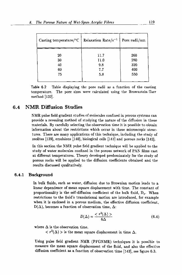
6. The Porous Nature of Wet-Spun Acrylic Fibres 119
Casting temperature/°C Relaxation Rate/s-1 Pore radii/nm
20 11.7 260 30 11.0 280 40 9.8 320 60 7.7 400 75 5.8 550
Table 6.2 Table displaying the pore radii as a function of the casting temperature. The pore sizes were calculated using the Brownstein-Tarr method [132].
6.4 NMR Diffusion Studies NMR pulse field gradient studies of molecules confined in porous systems can provide a revealing method of studying the nature of the diffusion in these materials. By carefully selecting the observation time it is possible to obtain information about the restrictions which occur in these microscopic struc- tures. There are many applications of this technique, including the study of zeolites 1139], emulsions [140], biological cells [141] and porous rocks [142].
In this section the NMR pulse field gradient technique will be applied to the study of water molecules confined in the porous network of PAN films cast at different temperatures. Theory developed predominately for the study of porous rocks will be applied to the diffusion coefficients obtained and the results discussed qualitatively.
6.4.1 Background
In bulk fluids, such as water, diffusion due to Brownian motion leads to a linear dependence of mean square displacement with time. The constant of proportionality is the self-diffusion coefficient of the bulk fluid, D3. When restrictions to the fluid's translational motion are introduced, for example when it is enclosed in a porous medium, the effective diffusion coefficient, D(A), becomes a function of observation time, 0:
D(A) =<r sý) > (6.4)
where 0 is the observation time. < r2(L) > is the mean square displacement in time A.
Using pulse field gradient NMR (PFGNMR) techniques it is possible to measure the mean square displacement of the fluid, and also the effective diffusion coefficient as a function of observation time [143], see figure 6.3.
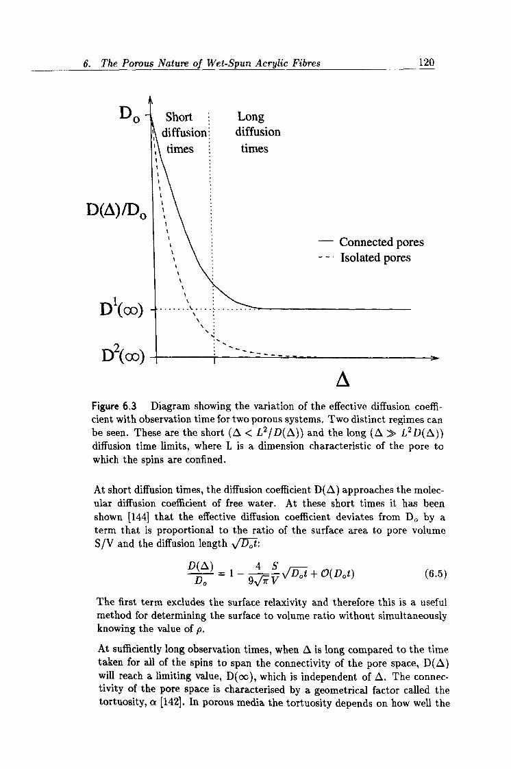
6. The Porous Nature of Wet-Spun Acrylic Fibres 120
Do Short Long diffusion diffusion times times
D(0)/D o
D1(oo)
2 co) ----- D(
Connected pores -- Isolated pores
A Figure 6.3 Diagram showing the variation of the effective diffusion coeffi- cient with observation time for two porous systems. Two distinct regimes can be seen. These are the short (0 < L2/D(t)) and the long (A » L2D(A. )) diffusion time limits, where L is a dimension characteristic of the pore to which the spins are confined.
At short diffusion times, the diffusion coefficient D(A) approaches the molec- ular diffusion coefficient of free water. At these short times it has been shown [144] that the effective diffusion coefficient deviates from Do by a term that is proportional to the ratio of the surface area to pore volume S/V and the diffusion length ot:
D(0) =1-4s Dot + ((Dot) (6.5)
Do 9, /ßr V
The first term excludes the surface relaxivity and therefore this is a useful method for determining the surface to volume ratio without simultaneously knowing the value of p.
At sufficiently long observation times, when A is long compared to the time taken for all of the spins to span the connectivity of the pore space, D(0) will reach a limiting value, D(oo), which is independent of A. The connec- tivity of the pore space is characterised by a geometrical factor called the tortuosity, a [1421. In porous media the tortuosity depends on how well the
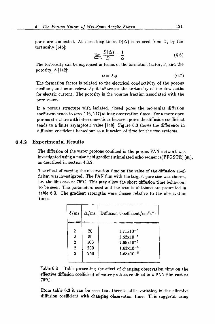
6. The Porous Nature of Wet-Spun Acrylic Fibres 121
pores are connected. At these long times D(z) is reduced from Do by the tortuosity [145]:
li D(A)
=1 (6.6)
The tortuosity can be expressed in terms of the formation factor, F, and the porosity, 0 [142]:
a= Fq (6.7)
The formation factor is related to the electrical conductivity of the porous medium, and more relevantly it influences the tortuosity of the flow paths for electric current. The porosity is the volume fraction associated with the pore space.
In a porous structure with isolated, closed pores the molecular diffusion coefficient tends to zero [146,1471 at long observation times. For a more open porous structure with interconnections between pores the diffusion coefficient tends to a finite asymptotic value [148]. Figure 6.3 shows the difference in diffusion coefficient behaviour as a function of time for the two systems.
6.4.2 Experimental Results
The diffusion of the water protons confined in the porous PAN network was investigated using a pulse field gradient stimulated echo sequence(PFGSTE) [96], as described in section 4.3.2.
The effect of varying the observation time on the value of the diffusion coef- ficient was investigated. The PAN film with the largest pore size was chosen, i. e. the film cast at 75°C. This may allow the short diffusion time behaviour to be seen. The parameters used and the results obtained are presented in table 6.3. The gradient strengths were chosen relative to the observation times.
S/ms 0/ms Diffusion Coefficient/ cm2 s-1
2 20 1.71x10⁻⁵ 2 50 1.62x10⁻⁵ 2 100 1.65x10⁻⁵ 2 200 1.63x10⁻⁵ 2 250 1.68x10⁻⁵
Table 6.3 Table presenting the effect of changing observation time on the effective diffusion coefficient of water protons confined in a PAN film cast at 75°C.
From table 6.3 it can be seen that there is little variation in the effective diffusion coefficient with changing observation time. This suggests, using
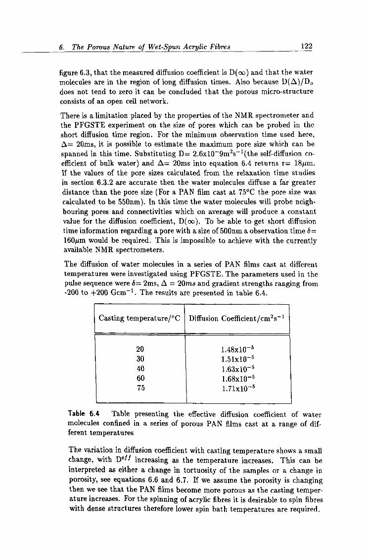
6. The Porous Nature of Wet-Spun Acrylic Fibres 122
figure 6.3, that the measured diffusion coefficient is D(oo) and that the water molecules are in the region of long diffusion times. Also because D(A)/Do does not tend to zero it can be concluded that the porous micro-structure consists of an open cell network.
There is a limitation placed by the properties of the NMR spectrometer and the PFGSTE experiment on the size of pores which can be probed in the short diffusion time region. For the minimum observation time used here, A. = 20ms, it is possible to estimate the maximum pore size which can be
spanned in this time. Substituting D= 2.6x10⁻⁹m 2s-1(the self-diffusion co- efficient of bulk water) and 0= 20ms into equation 6.4 returns r= 18µm. If the values of the pore sizes calculated from the relaxation time studies in section 6.3.2 are accurate then the water molecules diffuse a far greater distance than the pore size (For a PAN film cast at 75°C the pore size was calculated to be 550nm). In this time the water molecules will probe neigh- bouring pores and connectivities which on average will produce a constant value for the diffusion coefficient, D(oo). To be able to get short diffusion time information regarding a pore with a size of 500nm a observation time ö= 1601im would be required. This is impossible to achieve with the currently available NMR spectrometers.
The diffusion of water molecules in a series of PAN films cast at different temperatures were investigated using PFGSTE. The parameters used in the pulse sequence were b= 2ms, A= 20ms and gradient strengths ranging from -200 to +200 Gem-1. The results are presented in table 6.4.
Casting temperature/°C Diffusion Coefficient /CM2S-1
20 1.48x10⁻⁵ 30 1.51x10⁻⁵ 40 1.63x10⁻⁵ 60 1.68x10⁻⁵ 75 1.71x10⁻⁵
Table 6.4 Table presenting the effective diffusion coefficient of water molecules confined in a series of porous PAN films cast at a range of dif- ferent temperatures
The variation in diffusion coefficient with casting temperature shows a small change, with Del f increasing as the temperature increases. This can be interpreted as either a change in tortuosity of the samples or a change in porosity, see equations 6.6 and 6.7. If we assume the porosity is changing then we see that the PAN films become more porous as the casting temper- ature increases. For the spinning of acrylic fibres it is desirable to spin fibres with dense structures therefore lower spin bath temperatures are required.
6. The Porous Nature of Wet-Spun Acrylic Fibres 123
6.5 SEM of Cast PAN Films Scanning electron microscopy is a major technique used for the study of the morphology of polymers. The micrographs are obtained by recording the secondary electrons scattered from the surface of the sample. The resolu- tion for SEM is of the order of tens of nanometres, which is far superior to anything obtained using optical microscopy. Information about the morphol- ogy can be obtained directly by analysing the fractured surfaces or etched specimens.
6.5.1 SEM Sample Preparation
In order to investigate the internal structure of polymer films it is of paramount importance to be able to preserve the as-coagulated morphology. The prob- lem is that cast films and indeed fibres tend to change their structure as a result of drying. For example, the internal structure of a saturated, porous acrylic fibre will collapse with time if left under atmospheric conditions. The aqueous non-solvent filling the pores will slowly evaporate causing changes in the surface tension of the fibre leading to deformation of the original structure. For an analytical technique such as SEM it is essential to have a micro-structure free from liquid. A method therefore is required to remove the non-solvent from the cast film and retain the internal morphology. This will allow a comparative study of the effect of coagulation temperature, or indeed other parameters, on the internal film structure. The procedure of freeze-drying is well-known method for preserving the na- ture of membrane structures at the time of freezing [281. It was chosen in these studies to retain the cast film structure of PAN. The method involves the following steps:
" The cast film, as prepared using the method outlined in section 6.2, is immersed in an acetone bath. The polar acetone replaces the water molecules in the porous structure.
" The PAN film is then immersed in a heptane bath. The more volatile non-polar heptane replaces the acetone and the film is ready to be freeze-dried.
" The samples are placed in a liquid nitrogen bath to freeze them. Smaller samples with well-defined edge morphologies can be selected by carefully breaking the frozen films.
" The chosen samples are then placed in the apparatus shown in fig- ure 6.4. Effective evaporation of any remaining liquid from the PAN films takes place at a temperature between -20°C and -30°C and a pressure of 10-2-10-3mbar. Dry ice, within a dewar flask, is used to obtain temperatures in the appropriate range. The samples are left to dry for 24 hours and the effectiveness of the process can be verified
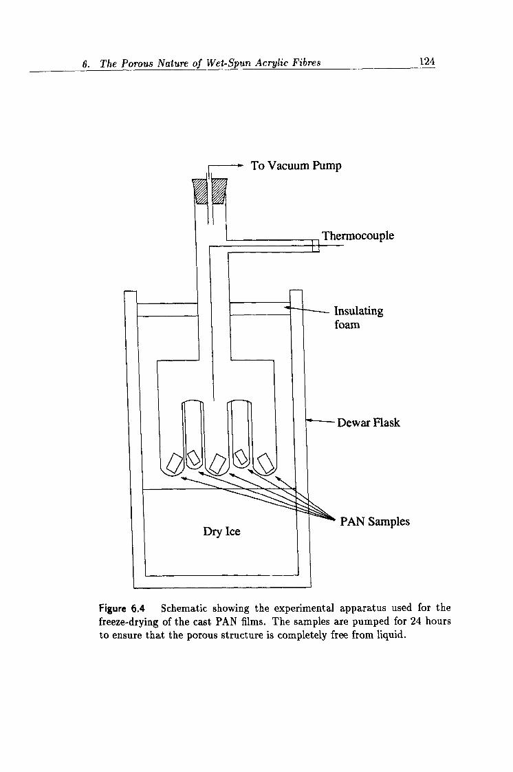
6. The Porous Nature of Wet-Spun Acrylic Fibres 124
mocouple
sulating am
)ewar Flask
'AN Samples
Figure 6.4 Schematic showing the experimental apparatus used for the freeze-drying of the cast PAN films. The samples are pumped for 24 hours to ensure that the porous structure is completely free from liquid.
T_ t 7_________ T. ____
6. The Porous Nature of Wet-Spun Acrylic Fibres 125
by monitoring the pressure as the flask warms. If there is no loss of vacuum then the process has finished.
The morphology of the PAN films can now be investigated using SEM.
6.5.2 Experimental
The micrographs were produced using a Hitachi S-3200 scanning electron microscope. This instrument is a conventional high resolution thermionic SEM, using a tungsten filament. It allows samples to be inserted directly into the chamber and observed in their natural state without the need for
coating the specimen with a contrast agent such as a heavy metal alloy or carbon.
Micrographs were taken of five PAN samples, coagulated at a range of dif- ferent temperatures, 20°C, 30°C, 40°C, 60°C and 75°C. The samples were investigated along the fractured edge to display the internal morphology developed during the coagulation process. Any evidence of dense skin for- mation was also probed.
6.5.3 Micrographs
Figures 6.5-6.9 display SEM micrographs of 13% PAN/NaSCN solutions cast at a range of temperatures. The differences in casting temperature is reflected by the change in scale of the porosity of the films. Note that the magnification is not consistent throughout the figures due to problems obtaining a good contrast.
Figure 6.5 displays the morphology of the PAN film cast at a low coagulation bath temperature of 20°C. The structure is fairly dense and it was difficult to resolve the fine structure of the porous network. The light and dark bands in the micrograph are attributed to uneven fracturing of the surface of the film after freeze drying.
In figures 6.6 and 6.7 it is possible to differentiate the pores from the polymer network. The pores(polymer lean phase) are represented by the dark areas and the polymer network(polymer rich phase)by the white/grey areas. The pore size is of the order of 10's of nanometres at this casting temperature, but it still difficult to resolve the morphology fully. However it is clear that the porosity has a scale less than 0.1 µm. Figure 6.8 shows more clearly a cellular structure, similar to that described by Knudsen [6]. The pore's size is seen to be increased relative to that found from the micrographs at lower casting temperatures. In this case the porosity has a scale of the order of 1µm or smaller.
Figure 6.9, which represents the film cast at 75°C, shows clearly a very open porous network. The packing of the polymer network is a lot less dense following the trend with temperature exhibited thus far. Some of the pores
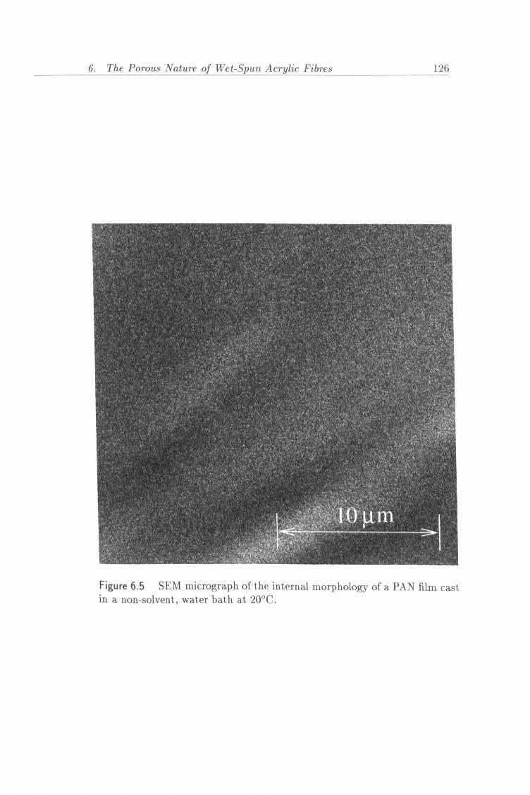
6. The Porous Nature of Wet-Spun Acrylic Fibres 126
Figure 6.5 SEM micrograph of the internal morphology of a PAN film cast in a non-solvent, water bath at 20°C.
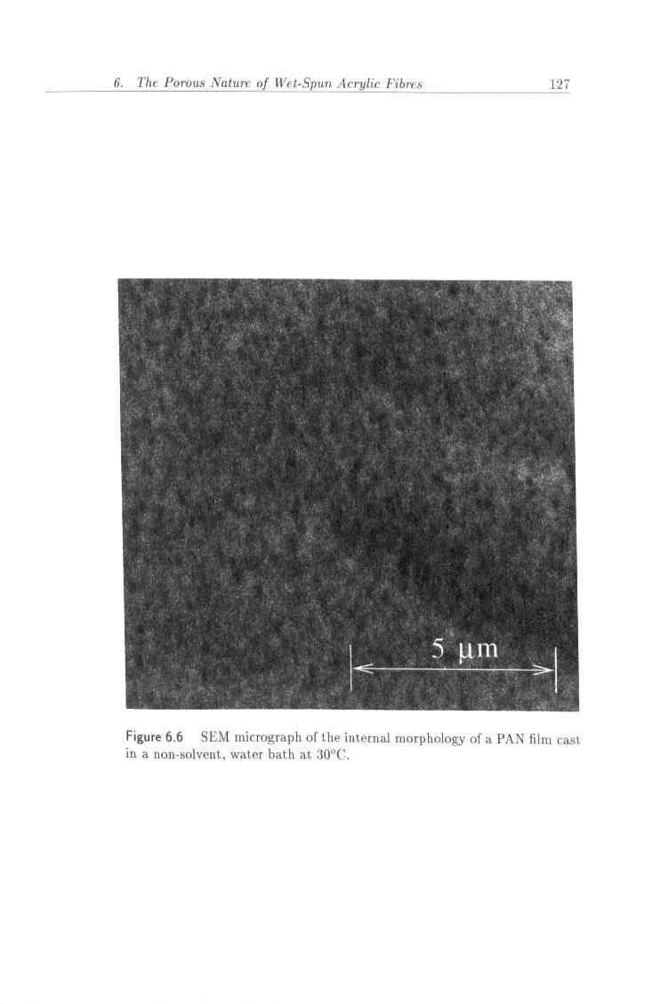
6. The Porous Nature of Wet-Spun Acrylic Fibres 127
Figure 6.6 SEM micrograph of the internal morphology of a PAN film cast in a non-solvent, water bath at 30°C.
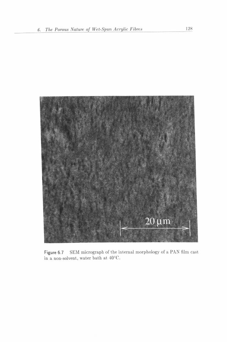
6. The Porous Nature of Wet-Spun Acrylic Fibres 128
Figure 6.7 SEM micrograph of the internal morphology of a PAN film cast in a non-solvent, water bath at 40°('.
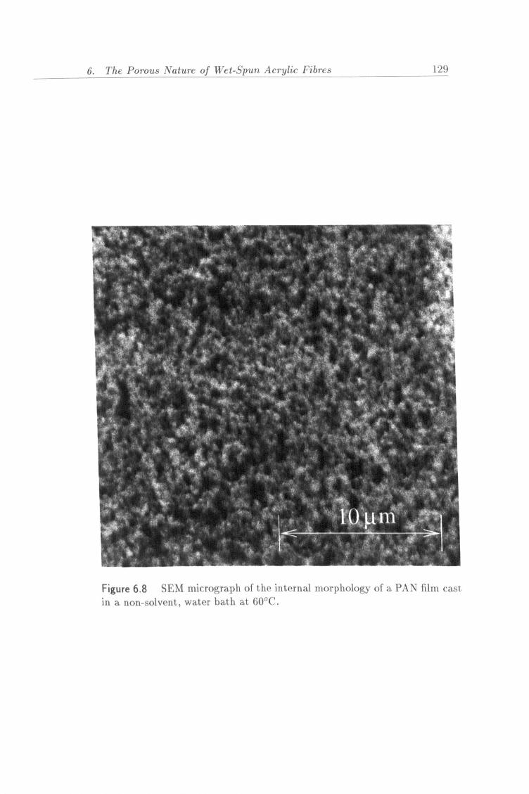
6. The Porous Nature of Wet-Spun Acrylic Fibres 129
Figure 6.8 SEM micrograph of the internal morphology of a PAN filrn cast in a non-solvent, water bath at 60°C.
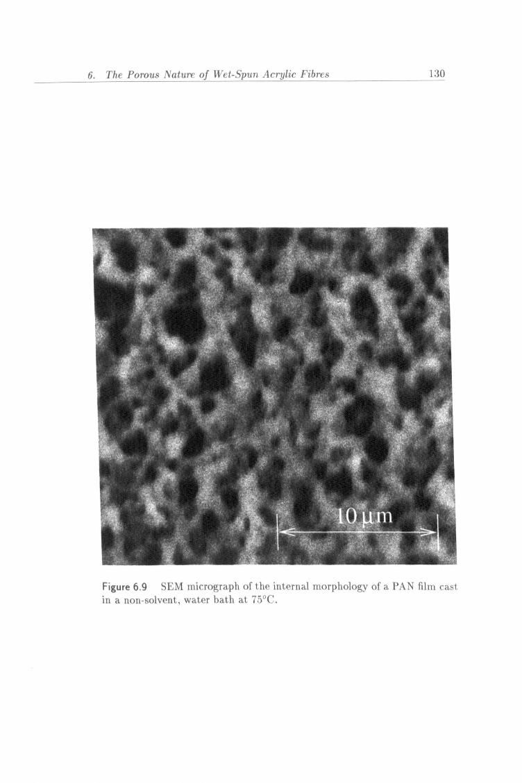
6. The Porous Nature of Wet-Spun Acrylic Fibres 130
Figure 6.9 5I': Nl nticrogral)h of the internal morphology of it PAN film cast in a non-solvent, water bath at 75°C.
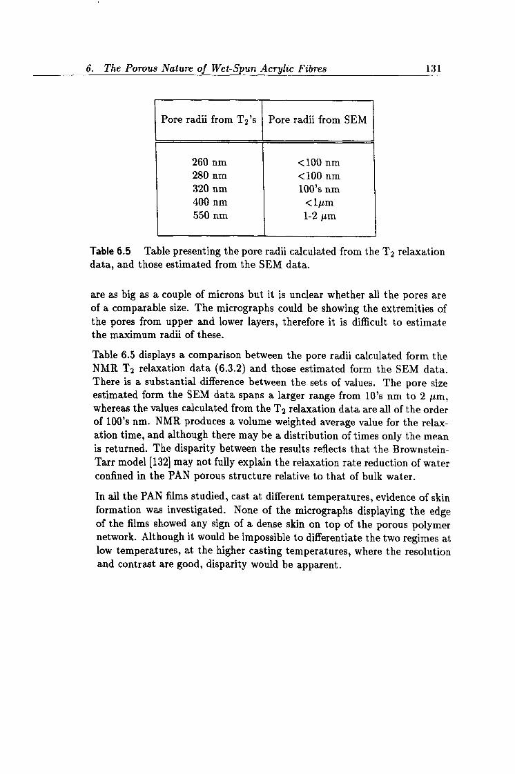
6. The Porous Nature of Wet-Spun Acrylic Fibres 131
Pore radii from T2's Pore radii from SEM
260 nm <100 nm 280 nm <100 nm 320 nm 100's nm 400 nm <1µm 550 nm 1-2 µm
Table 6.5 Table presenting the pore radii calculated from the T2 relaxation data, and those estimated from the SEM data.
are as big as a couple of microns but it is unclear whether all the pores are of a comparable size. The micrographs could be showing the extremities of the pores from upper and lower layers, therefore it is difficult to estimate the maximum radii of these.
Table 6.5 displays a comparison between the pore radii calculated form the NMR T2 relaxation data (6.3.2) and those estimated form the SEM data. There is a substantial difference between the sets of values. The pore size estimated form the SEM data spans a larger range from 10's nm to 2 µm, whereas the values calculated from the T2 relaxation data are all of the order of 100's nm. NMR produces a volume weighted average value for the relax- ation time, and although there may be a distribution of times only the mean is returned. The disparity between the results reflects that the Brownstein- Tarr model [132] may not fully explain the relaxation rate reduction of water confined in the PAN porous structure relative to that of bulk water.
In all the PAN films studied, cast at different temperatures, evidence of skin formation was investigated. None of the micrographs displaying the edge of the films showed any sign of a dense skin on top of the porous polymer network. Although it would be impossible to differentiate the two regimes at low temperatures, at the higher casting temperatures, where the resolution and contrast are good, disparity would be apparent.
Chapter 7 Conclusions
This concluding chapter summarizes the interpretations of the work de- scribed in the preceding four experimental chapters of this thesis. The first two of these preceding chapters show how nuclear magnetic resonance can be used to provide background information about the structure and interactions taking place in the PAN/NaSCNaq. system. A substantial amount of this NMR relaxation and self diffusion data was also used for the development of the NMR imaging experiment described in chapter 5. This work forms the main body of the thesis and the diffusion model used therein accurately describes the behaviour of the phase separating PAN solution. Chapter 6 supplements some of the ideas presented in the previous chapters by using scanning electron microscopy to show the structural variations which occur in phase separated PAN.
7.1 NMR Relaxation Studies of PAN solutions Bulk 1H NMR relaxation studies were carried out over a wide range of concentrations and temperatures to probe the molecular dynamics of the two proton containing species, polyacrylonitrile and water, which are con- stituents of the polymer solution studied in this thesis.
Traditional NMR methods were employed to collect the relaxation data. The longitudinal relaxation data was acquired using the inversion recovery pulse sequence whereas the transverse relaxation was acquired using the C arr- Purcell- Meiboom- Gill method. Good agreement was obtained between the two independent fitting procedures utilized to compute the relaxation parameters, see tables 3.1 and 3.2. Both these algorithms exhibited optimum results by implementing biexponential fitting routines. For a particular data-set the relaxation times of the two components of the biexponential were found to differ considerably and therefore the curve could be reproduceably resolved into its two constituents. The relative amplitudes of the two components showed good agreement for both the transverse and longitudinal relaxation data. These amplitudes were found to directly reflect the relative proton contents of the PAN and the water molecules over the full concentration and temperature range studied. Tables 3.4 and 3.6 compare the percentage amplitude of the faster decaying component, for T1 and T2 relaxation respectively, with the calculated percentage of protons attached to the PAN chains in the system. Good agreement is found for both modes of relaxation. The faster decaying component, which has a relaxation time of the order of tens of milliseconds, was therefore assigned to the larger and hence slower moving PAN macromolecule. Whereas the slower relaxing
132
7. Conclusions 133
component, with a relaxation time of the order of hundreds of milliseconds, could be assigned to the more mobile water molecules.
Investigations of temperature and concentration variations of relaxation times can provide information regarding the nature of any structural phase tran- sitions which may be occurring within the polymer solution over the range studied. For the PAN solutions studied here there is a steady increase in both longitudinal and transverse relaxation times as the temperature is in- creased or the concentration is decreased. This gradual change suggests that no sudden phase changes occur in the bulk solution over the ranges studied. Such transitions would lead to major changes in the magnitude of the relax- ation times at some critical temperature and/or concentration. Instead the PAN solutions remain homogeneous throughout the range studied, and this can be visibly confirmed by the lack of turbidity even at the concentration and temperature extremes studied.
The concentration variation of the relaxation times provides us with some insight into the nature of the interactions taking place within the PAN so- lution. The faster relaxation of the PAN protons shows little variation with increasing PAN concentration, suggesting that these local motions are not influenced much by polymer entanglements. The water relaxation rate is affected more markedly and as was proposed by Edwards et al. [24], the reduction in magnitude compared to bulk water can be attributed to the water breaking effect of the cyanate anion. This mechanism allows the, now free, water molecules to interact with the nitrile groups attached to the PAN chains. The water relaxation decreases with increasing PAN concentration and this reflects the increasing viscosity of the solution. The magnitude of the PAN relaxation times and the trends that they exhibit with concentra- tion suggest a species with a high degree of local motion. This is consistent with the representation of a polymer held in solution as a series of random coils, each coil-like conformation being one of the possible rotational isomeric states of the polymer chain. The aqueous sodium thiocyanate solution, in which the PAN is dissolved, allows rapid fluctuations between these states, and can thus be described as a "good" solvent for polyacrylonitrile.
The thermal dependences of the relaxation times also provide information regarding the mobility of the PAN/NaSCNaq. system. Comparing the trends of the transverse and longitudinal relaxation times for the PAN protons, it can be seen that both show an increase in value with increasing temperature. By comparing this to the BPP model for isotropic motion in a liquid sample it can be seen that both the PAN and the water protons fall into the region categorized as rapid molecular motion. This is consistent with our picture of PAN adopting a mobile random coil arrangement in the system.
7. Conclusions
7.2 Self Diffusion Studies
134
Self diffusion studies of polymer solutions have been extensively used to ob- tain information regarding the translational molecular motion of both the polymer chains and the solvent molecules. A NMR pulsed field gradient stimulated echo technique was used to acquire the echo attenuation data. This method was chosen in preference to the more widely used spin echo sequence due to the magnetization being stored in the longitudinal direc- tion, rather than in the transverse plane. For systems where T1 »T2 this leads to a considerable gain in signal amplitude. An unwanted addition to the pulsed field gradients applied to the sample on the MARAN-20 were background gradients. These had quite a large effect on the echo attenua- tion data acquired in these studies and therefore it was necessary to account for this effect in the analysis of the data. A novel fitting procedure was developed and implemented which allowed accurate values of the diffusion coefficient to be obtained from data acquired in the presence of background gradients. The weighted second order polynomial fitting program gave not only reproduceable values for the diffusion coefficient but also estimates of the strength of the background gradients. This proved to be an extremely valuable tool especially for the fitting of the slower PAN diffusion data.
As is the case with many polymer/solvent systems a reduction in the diffusion coefficient of the solvent with respect to that of pure solvent was exhibited in the PAN/NaSCNa, q, system. This deviation was seen to increase as the amount of PAN in the system was increased. A corresponding increase in the activation energy with increasing PAN concentration was also seen. Many models have been developed over the years to attempt to explain this phenomenon and some of these were applied in the discussion in chapter 4 in an attempt to explain the reduction of the value of the diffusion coefficient of water in the PAN/NaSCNaq. system. This analysis is intended to give an insight into the possible mechanisms which contribute to this phenomena rather than give a comprehensive review of the application of the available theories.
The Mackie and Meares model [75] which holds for very small solvent molecules is unsuccessful in fitting the experimental data. The curve predicted by the model is seen to deviate from the data points as the PAN concentration increases. This model, which is system independent and is based purely on obstruction effects, has proved successful in modelling systems where hydro- dynamic interactions are weak. In our system it appears that the obstruction mechanism does not solely describe the diffusion process and that there are other contributing factors present. This provides evidence for solvent poly- mer interactions with the highly polar nitrile groups undoubtedly playing a key role in this.
The free volume model of Yasuda [79], which is based on the work of Fu- jita [2}, produces good fits for the experimental diffusion data returning a value for the free volume parameter of B, /fu, =4.7. This parameter gives
7. Conclusions 135
a measure of the size of the solvent species. The exhibited behaviour can be explained because the free volume contributed by the polymer chains is believed to be much smaller than that contributed by the solvent molecules. Therefore this leads to a decrease in the value of the solvent's diffusion co- efficient with increasing polymer concentration. Free volume behaviour is thought to replace hydrodynamic interactions as the dominant factor as the concentration of polymer in the system is increased.
The hydrodynamic "universal" model proposed by Phillies and the scaling model proposed by Petit can be treated concurrently. The two models, al- though having different theoretical origins produce comparable results. The "universal" model returns two parameters, the prefactor a, which is related to the size of the diffusant, and the scaling exponent, v, which is a character- istic of the system (0.5<_ v <_1.0). The value for v returned from the fitting
of the experimental data classifies PAN as a small MW polymer, which is the case. The Petit model returns two fitting parameters v, which is a mea- sure of how good the solvent is and a, which is equal to kß2, where k is the jumping frequency and /3 is a constant for a given polymer system. The value of v=0.66 is consistent with a "goodish" solvent according to the def- initions that v=1.0 for a0 solvent, v=0.75 for a good solvent and v=0.5 for a marginal solvent. This agrees well with the predictions of the nature of the solvent from the NMR relaxation data, i. e. a good solvent. The diffusion coefficient of the solvent water molecules was also observed as a function of temperature. The diffusion coefficients as expected increased with increasing temperature, reflecting the increase in translational mobility. There was a corresponding increase in the activation energy for self diffusion as the PAN concentration was increased. So as the volume occupied by PAN molecules is increased it becomes more demanding for the water molecules to diffuse. If the free volume model is used this can be explained by the theory that polymer molecules contribute less free volume than water molecules for solvent diffusion to take place.
The diffusion coefficient of PAN in aqueous NaSCN solutions was studied as a function of increasing polymer concentration. Although these results are less comprehensive, mainly due to the difficulty in measuring the mobility of the relatively slow moving polymer chains, they exhibit similar trends to the solvent diffusion. The measured PAN diffusion coefficient was seen to decrease in value as the PAN concentration was increased. Although the trend was not fitted due to the uncertainty in the measurements, a exponential function similar to those used to fit the solvent diffusion could be used. Those mechanisms which are thought to contribute to the solvent diffusion also could play a part in the diffusion of the PAN molecules.
7. Conclusions 136
7.3 NMR Study of PAN Coagulation
The chapter which forms the main body of the work presented in this thesis is
concerned with the non solvent induced phase separation of PAN/NaSCNa,,.
solutions. The process was monitored using one dimensional 1H NMR imag- ing and the resulting time dependent concentration profiles were modelled by solving the diffusion equation for the appropriate initial and boundary
conditions.
The one-dimensional NMR imaging technique is a valuable method for mon- itoring the transport of proton containing species in single or multiphase systems. By using this method to monitor a PAN solution after the addi- tion of a suitable NMR inactive non-solvent it was possible to monitor the
phase separation process which takes place. Careful selection of the NMR
parameters allowed the projection of the solvent proton concentration onto a one dimensional profile. Monitoring the time evolution of the concentration profiles produced a unique quantitative way of studying the transport of the
solvent molecules out of the polymer solution. The solvent/non-solvent ra- tio is critical to the phase of the system and as the ratio decreases the two phase region of the ternary phase diagram will eventually be reached and the system will phase separate.
The evolution of the concentration profiles was modelled by solving Fick's diffusion equation using the relevant initial and boundary conditions. A semi-infinite medium was assumed and an initial sloped boundary condition was implemented to take account of the projection of the meniscus. This so- lution provided an accurate representation of the initial shape of the profile. The evolved profiles were each fitted using this solution and the magnitude of the fitting parameter fm*n confirmed that good fits were being produced.
The diffusion model fitted the profiles to three physical parameters: Co, D1
and D2. Essentially Co, which represents the initial concentration of water protons in the solution, provides another test to see how well the model fits the data. The value of Co remained at an almost constant value (taking
account of S/N) upto a time of approximately 70 minutes, confirming the applicability of the model. At times greater than this, when the value of Co decreases with time, the semi-infinite model becomes less effective.
The parameter D2 represents the average diffusion coefficient for water pro- tons in the area initially occupied by the non-solvent D20. The value re- turned for each diffusion profile decreases as the coagulation time increases. This behaviour can be explained by considering the local environment that the water molecules have diffused into. Initially the water molecules will be in an environment much like that experienced in pure liquid water and hence the diffusion coefficient tends to that of bulk water at time=O. As the coagulation time increases the water diffusion coefficient decreases and this can be explained by the increasing amount of NaSCN diffusing from the PAN entity. The presence of the salt decreases the diffusion coefficient of
7. Conclusions 137
the water and figure 5.20 shows that towards the latter stages of the experi- ment this tends towards a value of 1x10⁻⁵cm2s-1 representing a concentrated NaSCNaq, solution.
The parameter D1 represents the average diffusion coefficient for water pro- tons in the area initially occupied by the 13% PAN solution. The value returned for each diffusion profile increases as the phase separation time progresses. Figure 5.20 displays this variation of D1 with coagulation time and a weighted straight line fit of the data. The data initially fluctuates upto a time of approximately 20 minutes, after which the data follows a trend and increases linearly with coagulation time. The weighted fit of the data can be extrapolated back to a coagulation time of zero and this reveals a diffusion coefficient of 1.9x10-scm2s-1. This is essentially a measure of is the average diffusion coefficient in the profile area 1. At the beginning of the experiment this is occupied solely by the PAN solution and therefore we would expect this value to be equal to the bulk diffusion coefficient of water in a PAN solution of this concentration. Bulk values for a number of PAN solutions were determined using the methods presented in chapter 4(In this case D = 4.2x10⁻⁶ cm2s-1). Our value is of the same magnitude as the bulk value but is less then half the size. It is reasonable to attribute this to the noise levels of the profile data rather than assign it to any physical phenomenon. The increase in D1 with time highlights the changes in the structure of the PAN solution as coagulation time increases. The PAN changes environment from a mobile random coil in solution to a rigid, porous polymer network. The water molecules move from the homogeneous polymer solution with a mobility inhibited by the polymer chains to the polymer lean phase where their mobility is that of water in a aqueous NaSCN solution. As more of the PAN phase separates then the average diffusion coefficient increases as more water molecules move to the mobile environment. This trend continues until all the PAN has phase separated and the water molecules reach a constant diffusion coefficient.
The presence of a dense skin has been shown to exist in the structure of wet spun PAN fibres, although the role of this skin is not completely understood. In the experiments demonstrated here the skin, if present, does not appear to cause an appreciable barrier to the solvent/non-solvent exchange across the interface.
The MARAN-20 provided a suitable environment for producing one dimen- sional profiles for the time evolution of the phase separation of polymer solu- tions. The semi-infinite model was applied to these profiles and it provided a robust fitting procedure for the process, producing diffusion coefficients of the expected magnitude. This work shows the application of NMR imaging to the study of polymer phase separation.
7. Conclusions 138
7.4 The Porous Nature of Wet-Spun Acrylic Fibres This chapter investigates the structure of PAN films cast in non-solvent baths at a series of temperatures. NMR relaxation and self diffusion experiments were used to investigate the nature of the water trapped within the resulting porous polymer networks. Scanning electron microscopy was also used to produce micrographs of the internal structure for comparison. Analysis of the NMR relaxation results using the Brownstein-Tarr model re- turned values for the pore radii in the PAN films ranging from 260 to 550nm. The pore sizes increase as the non-solvent bath temperature is raised. This trend is expected and has been exhibited in previous studies [6]. The struc- ture of the films was investigated using SEM and from the resulting micro- graphs the pore sizes were estimated for comparison. This exercise produced pore sizes ranging from less than 100nm at the lowest bath temperature to greater than 2µm at the higher temperatures. When estimating these sizes it is natural to focus on the largest pores. The relaxation data, on the other hand, returns a volume weighted average for the pore size, and therefore represents a more accurate measure of the porosity of the films.
Bibliography
[1] N. Bloembergen, E. M. Purcell, and R. V. Pound. Relaxation effects in nuclear magnetic resonance. Physical Review, 73(7): 679-712,1948.
[2] H. Fujita. Diffusion in Polymer Solutions. Advances in Polymer Sci-
ence, 3: 1,1961.
[3] G. D. J. Phillies. Dynamics of polymers in concentrated solutions - The
universal scaling equation derived. Macromolecules, 20(3): 558,1987.
[4] A. Ziabicki. Fundamentals of Fibre Formation. John Wiley and Sons, 1976.
[5] G. Henrici-Olive and S. Olive. Molecular interactions and macroscopic properties of polyacrylonitrile and model substances. Advances in Polymer Science, 32: 128,1979.
[6] J. P. Knudsen. The influence of coagulation variables on the structure and physical properties of an acrylic fibre. Textile Research Journal, 33: 13,1963.
[7] S. H. Cho, J. S. Park, S. M. Jo, and I. J. Chung. Influence of ZnC12 on the structure and mechanical properties of polyacrylonitrile fibres. Polymer International, 34: 333,1994.
[8] J. P. Bell and J. H. Dumbleton. Changes in the structure of wet-spun acrylic fibres during processing. Textile Research Journal, 41: 196,1971.
[9] R. W. Moncrieff. Man Made Fibres. Newnes Butterworths, 1975.
[10] H. F. Mark. Encyclopedia of Polymer Science and Engineering. John Wiley and Sons Ltd., 1985.
[11] R. C. Houtz. Textile Research Journal, 20: 786,1950.
[12] A. M. Saum. Intermolecular association in organic nitriles; The CN dipole pair bond. Journal of Polymer Science, 42: 57,1960.
[13] S. Rosenbaum. Polyacrylonitrile fibre behaviour Mechanisms of tensile response. Journal of Applied Polymer Science, 9: 2071,1965.
[14] Xiao-Ping Hu. The molecular structure of polyacrylonitrile fibres. Journal of Applied Polymer Science, 62: 1925,1996.
[15] M. Murano and R. Yamadera. Studies on the tacticity of polyacryloni- trile. II. High resolution NMR spectra of 2,4 dicyanopentanes. Journal of Polymer Science: A-1,5: 1855,1967.
139
BIBLIOGRAPHY 140
[16] B. G. Frushour. Water as a melting point depressant for acrylic poly- mers. Polymer Bulletin, 7: 1,1982.
[17] K. Kamide, H. Yamazaki, K. Okajima, and K. Hikichi. Pentad tacticity of polyacrylonitrile polymerised by 'y radiation on urea-acrylonitrile canal complex at 78°C. Polymer Journal, 17: 1291,1985.
[18] M. Minagawa, H. Yamada, K. Yamaguchi, and F. Yoshi. -y-ray irra- diation canal polymerisation conditions ensuring highly stereoregular polyacrylonitrile. Macromolecules, 25: 504,1992.
[19] G. Hinrichsen. Structural changes of drawn polyacrylonitrile during annealing - Two phase structure. Journal of Polymer Science, Part C, 38: 303,1972.
[20] R. J. Hobson and A. H. Windle. Crystalline structure of atactic poly- acrylonitrile. Macromolecules, 26: 6903,1993.
[21] R. Chiang, J. Brandrup, and E. H. Immergut. Polymer Handbook. John Wiley and Sons Ltd., 1966.
[22] B. E. Geller and N. P. Eftina. The properties of polyacrylonitrile solu- tions in inorganic salts. Khimicheskie Volokna, 4: 10,1961.
[23] A. R. Hoskins, H. G. Edwards, and A. F. Johnson. Vibrational spectro- scopic studies of polyacrlonitrile-co vinyl acetate in aqueous solutions containing metal ions - mechanism of the dissolution process. Polymer Communications, 32: 89,1989.
[241 H. G. M. Edwards, A. R. Hoskins, A. F. Johnson, and I. R. Lewis. Raman
spectroscopic studies of the polyacrylonitrile-zinc complexes in aqueous solutions of zinc chloride and bromide. Polymer International, 30: 25, 1993.
[25] M. Hattori, H. Yamazaki, M. Saito, K. Hisatani, and K. Okajima. NMR study of the dissolved state of polyacrylonitrile in various sol- vents. Polymer Journal, 28(7): 594,1996.
[26] S. J. Law and S. K. Mukhopadhyay. Investigation of wet-spun acrylic fibre morphology by membrane technology techniques. Journal of Ap- plied Polymer Science, 62: 33,1996.
[27] D. R. Paul. Diffusion during the coagulation step of wet spinning. Journal of Applied Polymer Science, 12: 383,1968.
[28] J. P. Craig, J. P. Knudsen, and V. F. Holland. Characterization of acrylic fibre structure. Textile Research Journal, 32: 435,1962.
[29] F. W. Altena, J. W. A. Smid, J. van den Berg, J. G. Wijmans, and C. A. Smolders. Diffusion of solvent from a cast cellulose acetate solution during the formation of skinned membranes. Polymer, 26: 1531,1985.
BIBLIOGRAPHY 141
[30] R. K. Harris. Nuclear Magnetic Resonance Spectroscopy. Longman Scientific and Technical, 1991.
[31] C. P. Slichter. Principles of Magnetic Resonance. Harper and Row, 1963.
[32] T. C. Farrar and E. D. Becker. Pulse and Fourier Transform NMR. Academic Press, 1971.
[33] B. P. Cowan. Nuclear Magnetic Resonance and Relaxation. Cambridge University Press, 1997.
[34] J. W. Hennel and J. Klinowski. Fundamentals of Nuclear Magnetic Resonance. Longman Scientific and Technical, 1993.
[35] V. C. McBrierty and K. J. Packer. Nuclear Magnetic Resonance in Solid Polmers. Cambridge University Press, 1993.
[36] J-. J. Delpuech. Dynamics of Solutions and Fluid Mixtures by NMR. Wiley, 1995.
[37] W. Pauli. Naturwissenschaften, 12: 741,1924.
[38] F. Bloch, W. W. Hansen, and M. Packard. Nuclear induction. Physical Review, 69: 127,1946.
[39] E. M. Purcell, H. C. Torrey, and R. V. Pound. Resonance absorption by nuclear magnetic moments in a solid. Physical Review, 69: 37,1946.
[40] F. Bloch. Nuclear induction. Physical Review, 70(7 - 8): 460-474,1946.
[41] E. L. Hahn. Spin echoes. Physical Review, 80(4): 580-594,1950.
[42] J. T. Arnold, S. S. Dharmatti, and M. E. Packard. Chemical effects on nuclear induction signals from organic compounds. Journal of Chem- ical Physics, 19: 507,1951.
[43] J. W. Cooley and J. W. Tukey. An alogorithm for the machine calcula- tion of complex Fourier series. Mathematics of Computation, 19: 297, 1965.
[44] I. J. Lowe and R. E. Norberg. Free-induction decays in solids. Physical Review, 107: 46,1957.
[45] R. R. Ernst and W. A. Anderson. Application of Fourier transform spectroscopy to magnetic resonance. Review of Scientific Instruments, 37: 93,1966.
[46] H. Y. Carr and E. M. Purcell. Effects of diffusion on free precession in nuclear magnetic resonance experiments. Physical Review, 94(3): 630- 638,1954.
BIBLIOGRAPHY 142
[47] E. 0. Stejskal and J. E. Tanner. Spin diffusion measurements: Spin echoes in the presence of a time dependent field gradient. Journal of Chemical Physics, 42(1): 288,1965.
[48] P. C. Lauterbur. Image formation by induced local interactions: Ex- amples employing nuclear magnetic resonance. Nature, 242: 190,1973.
[49] P. Mansfield and P. K. Grannell. NMR `diffusion' in solids. Journal of Physics C, 6: L422,1973.
[50] P. Mansfield and A. A. Maudsley. Medical imaging by NMR. British Journal of Radiology, 50: 188,1977.
[51] E. R. Andrew, P. A. Bottomley, W. S. Hinshaw, G. N. Holland, W. S. Moore, and C. Simaroj. NMR images by the multiple sensitive point method: Application to larger biological systems. Physics in Medicine
and Biology, 22: 971,1977.
[52] G. E. Uhlenbeck and S. Goudsmit. Naturwissenschaften, 13: 953,1925.
[53] E. Fukushima and S. B. W. Roeder. Experimental Pulse NMR: A Nuts and Bolts Approach. Addison-Wesley, London, 1981.
[54] M. L. Martin, G. J. Martin, and J-. J. Delpuech. Practical NMR Spec- troscopy. Heyden and Son Ltd., 1980.
[55] D. I. Hoult. The NMR receiver: A description and analysis of design. Progress in NMR Spectroscopy, 12: 41,1978.
[56] R. Kubo and K. Tomita. A general theory of magnetic resonance absorption. Journal of the Physical Society of Japan, 9: 888,1954.
[57] D. Canet, G. C. Levy, and I. R. Peat. Time saving in 13C spin-lattice relaxation measurements by inversion recovery. Journal of Magnetic Resonance, 18: 199,1975.
[58] S Meiboom and D. Gill. Modified spin-echo methods for measuring nuclear relaxtion times. Review of Scientific Instruments, 29: 688,1958.
[59] P. S. Belton, R. R. Jackson, and Packer K. J. Pulsed NMR studies of water in striated muscle. I. Effects of freezing and transverse nuclear spin relaxation times. Biochimica et Biophysica Acta., 286: 16,1972.
[60] P. S. Belton, Packer K. J., and T. C. Sellwood. Pulsed NMR studies of water in striated muscle. II. Spin-lattice relaxation times and the dy- namics of the non-freezing fraction of water. Biochimica et Biophysica Acta., 304: 56,1973.
[61] P. S. Belton and Packer K. J. Pulsed NMR studies of water in striated muscle. III. The effects of water content. Biochimica et Biophysica Acta., 354: 305,1974.
BIBLIOGRAPHY 143
[62] H. D. Van Liew. Semilogarithmic plots of data which reflect a contin- uum of exponential processes. Science, 138: 682,1962.
[63] W. H. Press, B. P. Flannery, S. A. Teukolski, and W. T. Vetterling. Nu-
merical recipes in C: The Art of Scientific Computing. Cambridge University Press, 1992.
[64] K. P. Whittall and A. L. Mackay. Quantitative interpretation of NMR
relaxation data. Journal of Magnetic Resonance, 84: 134,1989.
[65] S. W. Provencher. A constrained regularization method for inverting data presented by linear algebraic or integral equations. Computer Physics Communications, 27: 213-227,1982.
[66] S. W. Provencher. CONTIN: a general purpose constrained regulariza- tion program inverting noisy linear algebraic and integral equations. Computer Physics Communications, 27: 229-242,1982.
[671 R. M. Kroeker and R. M. Henkelman. Analysis of biological NMR relax- ation data with continuous distributions of relaxation times. Journal of Magnetic Resonance, 69: 218,1986.
[68] E. D. von Meerwall. Self diffusion in polymer systems, measured with field gradient spin-echo NMR methods. Advances in Polymer Science, 54: 1,1984.
[69] A. H. Murh and J. M. V. Blanshard. Diffusion in gels. Polymer, 23: 1012, 1982.
[70] M. Tirrell. Polymer self diffusion in entangled systems. Rubber Chem- istry and technology, 57(3): 523,1984.
[71] P. T. Callaghan. Pulsed field gradient NMR as a probe of liquid state molecular organization. Australian Journal of Physics, 37(4): 359,1984.
[72] F. D. Blum. Pulsed field gradient spin-echo NMR spectroscopy. Spec- troscopy, 1(5): 32,1986.
[73] P. Stilbs. Fourier transfrom pulsed field gradient spin-echo studies of molecular diffusion. Progress in NMR Spectroscopy, 19: 1,1987.
[74] J. Crank. The Mathematics of Diffusion. Oxford Science Publications, 1975.
[75] J. S. Mackie and P. Meares. The diffusion of electrolytes in cation exchange resin membrane. 1. Theoretical. Proceedings of the Royal Society of London A, 232: 498,1955.
[76] R. A. Waggoner, F. D. Blum, and J. M. D. MacElroy. Dependence of the solvent diffusion coefficient on concentration in polymer solutions. Macromolecules, 26(25): 6841,1993.
BIBLIOGRAPHY 144
[77] R. D. Boss, E. O. Stejskal, and J. D. Ferry. Self diffusion in high molecular weight polyisobutylene-benzene mixtures determined by the pulsed field gradient spin-echo method. Journal of Physical Chemistry, 71(5): 1967,1501.
[78] A. Bandis, P. T. Inglefield, A. A. Jones, and W-Y. Wen. A nuclear magnetic resonance study of dynamics in toluene-polyisobutylene so- lutions: 1. Penetrant diffusion and Fujita theory. Journal of Polymer Science: Part B-Polymer Physics, 33: 1495,1995.
[79] H. Yasuda, C. E. Lamaze, and L. D. Ikenberry. Permeability of solutes through hydrated membranes. Part I. Diffusion of sodium chloride. Die Makromolekulare Chemie, 118: 19,1968.
[80] J. S. Vrentas and J. L. Duda. Diffusion in polymer-solvent systems. I Re-examination of the free volume theory. Journal of Polymer Science: Part B-Polymer Physics, 15: 403,1977.
[81] J. S. Vrentas and J. L. Duda. Diffusion in polymer-solvent systems. II A predictive theory for the dependence of diffusion coefficients on temperature, concentration and molecular weight. Journal of Polymer Science: Part B-Polymer Physics, 15: 417,1977.
[821 J. S. Vrentas and J. L. Duda. Diffusion in polymer-solvent systems. III. Construction of Deborah number diagrams. Journal of Polymer Science: Part B-Polymer Physics, 15: 441,1977.
[83] R. I. Cukier. Diffusion of Brownian spheres in semidilute polymer so- lutions. Macromolecules, 17(2): 252,1984.
[84] K. F. Freed and S. F. Edwards. Polymer vicosity in concentrated solu- tions . Journal of Chemical Physics, 61(9): 3626,1974.
[85] P-G. de Gennes. . Macromolecules, 9: 594,1976.
[86] G. D. J. Phillies. The hydrodynamic scaling model for polymer self diffusion. Journal of Physical Chemistry, 93(13): 5029,1989.
[87] P. G. de Gennes. Scaling Concepts in Polymer Physics. Cornell Uni- versity Press, 1979.
[88] J-M. Petit, B. Roux, X. X. Zhu, and P. M. MacDonald. A new phys- ical model for the diffusion of solvents and solute probes in polymer solutions. Macromolecules, 29: 6031,1996.
[89] D. W. Williams, E. F. W. Seymour, and R. M. Cotts. A pulsed gradi- ent multiple spin echo NMR technique for measuring diffusion in the presence of background magnetic field gradients. Journal of Magnetic Resonance, 31: 271,1978.
BIBLIOGRAPHY 145
[90] L. L. Latour, L Limin, and C. H. Sotak. Improved PFG stimulated echo method for the measurement of diffusion in inhomogeneous fields. Journal of Magnetic Resonance, Series B, 101: 72,1993.
[91] E. J. Fordham, S. J. Gibbs, and L. D. Hall. Partially restricted diffu- sion in a permeable sandstone: Observations by stimulated echo PFG NMR. Magnetic Resonance Imaging, 12(2): 279,1994.
[92] R. F. Karlicek and I. J. Lowe. A modified pulsed gradient technique for measuring diffusion in the presence of large background gradients. Journal of Magnetic Resonance, 37: 75,1980.
[93] H. C. Torrey. Bloch equations with diffusion terms. Physical Review, 104: 563,1956.
[94] D. C. Douglass and D. W. McCall. Diffusion in paraffin hydrocarbons. Journal of Physical Chemistry, 62: 1102,1958.
[95] D. W. McCall, D. C. Douglass, and E. W. Anderson. Self diffusion stud- ies by means of NMR spin-echo techniques. Berichte der Bunsenge- sellschaft Physikalische Chemie, 67(3): 336,1963.
[96] J. E. Tanner. Use of the stimulated echo in NMR diffusion studies. Journal of Chemical Physics, 52(5): 2523,1970.
[97] K. R. Harris, R. Mills, P. J. Back, and D. S. Webster. An improved NMR spin-echo apparatus for the measurement of self diffusion coefficients: The diffusion of water in aqueous electrolyte solutions. Journal of Magnetic Resonance, 29: 473,1978.
[98] H. Weingärtner. Self diffusion in liquid water a reassessment. Zeitschrift
, für Physikalische Chemie Neue Folge, 132: 129,1982.
[99] R. Mills. Self diffusion in normal and heavy water in the range 1-45°C. Journal of Phsical Chemistry, 77(5): 685,1973.
[100] M. I. Hrovat and C. G. Wade. NMR pulsed gradient diffusion mea- surements. I. Spin-echo stability and gradient calibration. Journal of Magnetic Resonance, 44: 62,1981.
[101] IDL Student Version 5.0,1997.
[102] J-M. Petit, X. X. Zhu, and P. M. MacDonald. Solute probe diffusion in aqueous solutions of poly(vinyl alcohol) as studied by pulsed gradient spin-echo NMR spectroscopy. Macromolecules, 29: 70,1996.
[103] S. C. Oh, Y. S. Wang, and Y-K. Yeo. Modelling and simulation of the coagulation process of polyacrylonitrile wet-spinning. Industrial Engineering: Chemical Research, 35: 4796,1996.
BIBLIOGRAPHY 146
[104] C. D. Han and L. Segal. A study of fibre extrusion in wet spinning. 1. Experimental determination of elongational viscosity. Journal of Applied Polymer Science, 14: 2973,1970.
[105] C. D. Han and L. Segal. A study of fibre extrusion in wet spinning. II. Effects of spinning conditions on fibre formation. Journal of Applied Polymer Science, 14: 2999,1970.
[106] J. R. Booth. Diffusion-limited coagulation in wet spun single filaments. American Chemical Society: Polymer Preprints, 7: 759,1966.
[107] G. Feio and J. P. Cohen-Addad. NMR approach to the kinetics of polymer crystallisation. 1. Cis-1,4-polybutadiene. Journal of Polymer Science: Part B-Polymer Physics, 26: 389,1988.
[108] G. Feio, G. Buntinx, and J. P. Cohen-Addad. NMR approach to the kinetics of polymer crystallisation. 1. Polydimethylsiloxane solutions. Journal of Polymer Science: Part B-Polymer Physics, 27: 1,1989.
[109] A. Viallat and S. Perez. NMR approach to properties of polymeric membranes. Kinetics of membrane formation. Journal of Polymer Sci-
ence: Part B-Polymer Physics, 31: 1567,1993.
[110] F-J. Tsai and J. M. Torkelson. Roles of separation mechanism and coarsening in the formation of poly(methyl methacrylate) asymmetric membranes. Macromolecules, 23: 775,1990.
[111] R. J. Young and P. A. Lovell. Introduction to Polymers. Chapman and Hall, 1991.
[1121 J. M. G. Cowie. Polymers: Chemistry and Physics of Modernn Materi-
als. Blackie Academic and Professional, 1991.
[1131 G. R. Strobl. The Physics of Polymers: Concepts for understanding their structures and behaviour. Springer-Verlag, 1996.
[1141 G. R. Strobl, J. T. Bendler, R. P. Kambour, and A. R. Shultz. Ther-
maIly reversible phase-separation in polystyrene poly(styrene-co- bromostyrene) blends. Macromolecules, 19: 2683,1986.
[115] C. Cohen, G. B. Tanny, and S. Prager. Diffusion controlled fromation of porous structures in ternary polymer solutions. Journal of Polymer Science: Part B-Polymer Physics, 17: 477,1979.
[116] B. F. Barton, J. L. Reeve, and A. J. McHugh. Observations on the dy- namics of nonsolvent-induced phase inversion. Journal of Polymer Science Part B-Polymer Physics, 35: 569,1997.
[117] S. J. Law and S. K. Mukhopadhyay. The construction of a phase dia- gram for a ternary system used for the wet spinning of acrylic fibres based on a linearized cloudpoint curve correlation. Journal of Applied Polymer Science, 65: 2131,1997.
BIBLIOGRAPHY 147
[118] R. M. Boom, T. van den Boomgard, J. W. A. van den Berg, and C. A. Smolders. Linearised cloudpoint curve correlation for ternary systems consisting of one polymer, one solvent and one non-solvent. Polymer, 34: 2348,1993.
[119] H. Strathmann and K. Kock. The formation mechanism of phase in-
version membranes. Desalination, 21: 241,1977.
[120] P. T. Callaghan. Principles of Nuclear Magnetic Resonance Mi- croscopy. Oxford Science Publications, 1991.
[121] H. S. Carslaw and J. C. Jaegar. Conduction of Heat in Solids. Oxford Science publications, 1986.
[122] Maple V Release 4,1996.
[123] S. A. McKelvey and W. J. Koros. Phase separation, vitrification and the manifestation of macrovoids in polymeric asymmetric membranes. Journal of Membrane Science, 112: 29,1996.
[124] C. A. Smolders. Ultrafiltration Membranes and Applications. Plenum Press, 1980.
[125] R. Hills. Self-Diffusion in Normal and Heavy Water in the range 1- 45°C. Journal of Physical Chemistry, 77: 685,1973.
[126] M. Takahashi, Y. Nukushina, and S. Kosugi. Effect of fibre forming conditions on the microstructures of acrylic fibre. Textile Research Journal, 34: 87,1964.
[127] S. L. Dart. Entropy stress study of various textile fibres. Textile Re- search Journal, 30: 372,1960.
[128] P. van de Witte. Phase separation processes in polymer solutions in relation to membrane formation. Journal of Membrane Science, 117: 1, 1996.
[129] H. F. Mark, N. M. Bikales, C. G. Overberger, and G. Menges. Encyclo- pedia of Polymer Science and Engineering: Volume 9. John Wiley and Sons, 1987.
[130] S. Loeb and S. Sourirajan. Sea water demineralisation by means of an osmotic membrane. Advances in Chemistry Series, 33: 117,1962.
[131] M. C. Cohen and K. S. Mendelson. Nuclear magnetic resonance and the internal geometry of sedimentary rocks. Journal of Applied Physics, 53(2): 1127,1982.
[132] K. R. Brownstein and C. E. Tarr. Importance of classical diffusion in NMR studies of water in bioloical cells. Physical Review A, 19: 2446, 1979.
BIBLIOGRAPHY 148
[133] K. R. Brownstein and C. E. Tarr. Spin-lattice relaxation in a system governed by diffusion. Journal of Magnetic Resonance, 26: 17,1977.
[134] H. J. Kim, R. K. Tyagi, A. E. Fouda, and K. Jonasson. The kinetic
study for asymmetric membrane formation via phase-inversion process. Journal of Applied Polymer Science, 62: 621,1996.
[135] A. J. Reuvers, J. W. A. van den Berg, and C. A. Smolders. Formation of membranes by means of immersion precipitation. Part I. A model to describe mass transfer during immersion precipitation. Journal of Membrane Science, 34: 45,1987.
[136] K. J. Packer. The effects of diffusion through locally inhomogeneous magnetic fields on transverse nuclear spin relaxation in heterogeneous systems. Proton transverse relaxation in striated muscle tissue. Journal
of Magnetic Resonance, 9: 483,1973.
[137] S. Davies and K. J. Packer. Pore-size distributions from NMR spin- lattice relaxation measurements of fluid saturated porous solids. 1. Theory and simulation. Journal of Applied Physics, 67: 3163,1990.
[138] M. D. Hurlimann, K. G. Helmer, L. L. Latour, and C. H. Sotak. Re- stricted diffusion in sedimentary rocks. Determination of surface-area- to-volume ratio and surface relaxivity. Journal of Magnetic Resonance series A, 111: 169,1994.
[139] S. S. Nivarthi and A. V. McCormick. Diffusion of coadsorbed molecules in zeolites- A pulsed field gradient NMR study. Journal of Physical Chemistry, 99(13): 4661,1995.
[140] K. J. Packer and C. Rees. Pulsed NMR studies of restricted diffusion. 1. Droplet size distributions in emulsions. Journal of Colloid and In- terface Science, 40(2): 206,1972.
[141] D. G. Cory and A. N. Garroway. Measurement of translational dis- placement probabilities by NMR: An indicator of compartmentation. Magnetic Resonance in Medicine, 14(3): 435,1990.
[142] P. N. Sen, L. M. Schwartz, P. P. Mitra, and B. I. Halperin. Surface relax- ation and the long time diffusion coefficient in porous media: Periodic geometries. Physical Review B, 49(1): 215,1994.
[143] E. 0. Stejskal. Spin-echo mesurement of self diffusion in colloidal sys- tems. Advances In Molecular Relaxation Processes, 3: 27-42,1972.
[144] P. P. Mitra, P. N. Sen, L. M. Schwratz, and P. Le Doussal. Diffusion propagator as a probe of the structure of porous media. Physical Re- view Letters, 68: 3555,1992.
BIBLIOGRAPHY 149
[145] D. L. Johnson, T. J. Plona, C. Scala, F. Pasierb, and H. kojima. Tortu- osity and acoustic slow waves. Physical Review Letters, 49(25): 1840, 1982.
[146] R. C. Wayne and R. M. Cotts. Nuclear magnetic resonance study of self- diffusion in a bounded medium. Physical Review, 151(1): 264,1966.
[147) R. C. Wayne and R. M. Cotts. Erratum. Physical Review, 159(2): 486, 1967.
[148] L. L. Latour, P. P. Mitra, R. L. Kleinberg, and P. Le Doussel. Time- dependent diffusion coefficient of fluids in porous media as aprobe of surface-to-volume ratio. Journal of Magnetic resonance A, 101: 342, 1993.
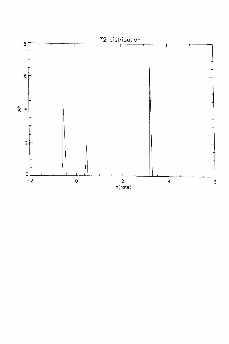
T2 distribution
w a
-2 In(rate)