new type curves for the analysis of pressure transient data of
111
NEW TYPE CURVES FOR THE ANALYSIS OF PRESSURE TRANSIENT DATA OF HORIZONTAL WELLS IN NON- NEWTONIAN FLUID RESERVOIRS 2011 NEW TYPE CURVES FOR THE ANALYSIS OF PRESSURE TRANSIENT DATA OF HORIZONTAL WELLS IN NON-NEWTONIAN FLUID RESERVOIRS A Thesis PRESENTED TO THE DEPARTMENT OF PETROLEUM ENGINEERING AFRICAN UNIVERSITY OF SCIENCE AND TECHNOLOGY In Partial Fulfillment of Requirements for the Award of Degree of MASTER OF SCIENCE By ADENUGA, KAZEEM ADEBOWALE, B.Sc. ABUJA, FCT. DECEMBER, 2011
-
Upload
khangminh22 -
Category
Documents
-
view
5 -
download
0
Transcript of new type curves for the analysis of pressure transient data of
NEW TYPE CURVES FOR THE ANALYSIS OF PRESSURE TRANSIENT DATA OF HORIZONTAL WELLS IN NON-NEWTONIAN FLUID RESERVOIRS
2011
NEW TYPE CURVES FOR THE ANALYSIS OF PRESSURE TRANSIENT DATA OF HORIZONTAL WELLS IN NON-NEWTONIAN FLUID RESERVOIRS
A Thesis
PRESENTED TO THE DEPARTMENT OF PETROLEUM ENGINEERING
AFRICAN UNIVERSITY OF SCIENCE AND TECHNOLOGY
In Partial Fulfillment of Requirements for the Award of Degree of
MASTER OF SCIENCE
By
ADENUGA, KAZEEM ADEBOWALE, B.Sc.
ABUJA, FCT.
DECEMBER, 2011

NEW TYPE CURVES FOR THE ANALYSIS OF PRESSURE TRANSIENT DATA OF HORIZONTAL WELLS IN NON-NEWTONIAN FLUID RESERVOIRS
2011
NEW TYPE CURVES FOR THE ANALYSIS OF PRESSURE TRANSIENT DATA OF HORIZONTAL WELLS IN NON-NEWTONIAN FLUID RESERVOIRS
By
ADENUGA Kazeem Adebowale
RECOMMENDED:
Dr. Alpheus Igbokoyi Committee Chair
Professor Djebbar Tiab Committee Member
Professor Godwin Chukwu Committee Member
APPROVED:
Chief Academic Officer
Date:
NEW TYPE CURVES FOR THE ANALYSIS OF PRESSURE TRANSIENT DATA OF HORIZONTAL WELLS IN NON-NEWTONIAN FLUID RESERVOIRS 2011
iii
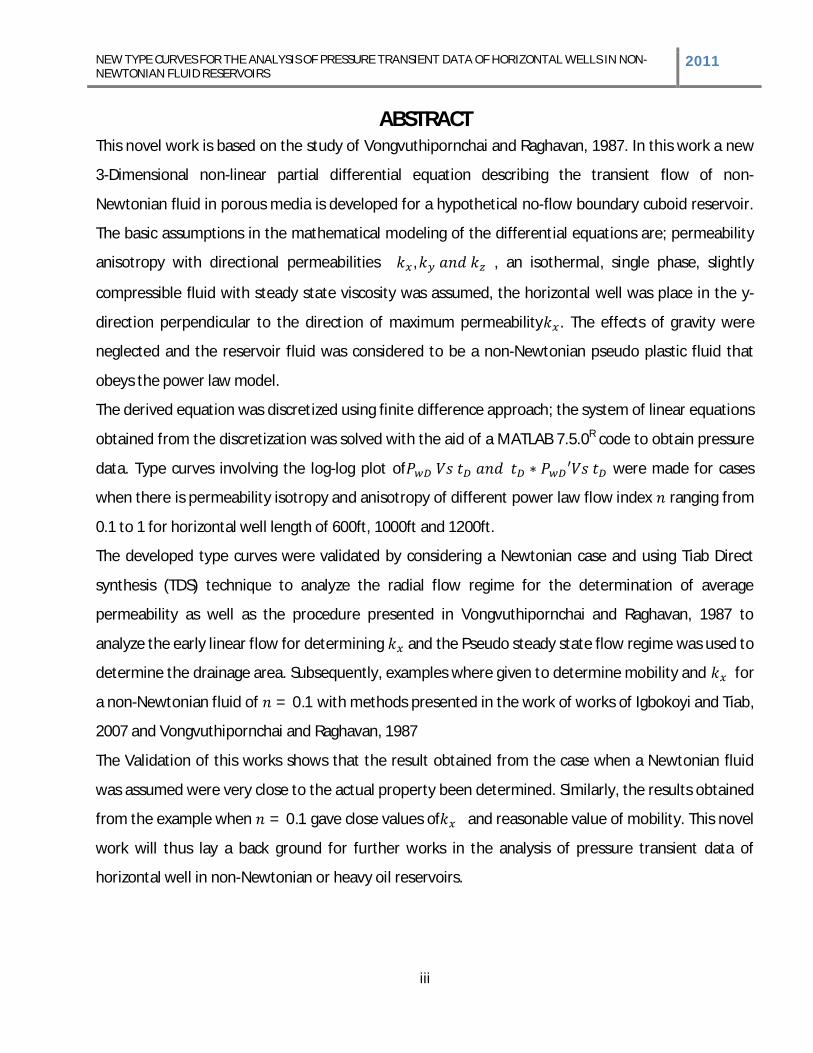
ABSTRACT This novel work is based on the study of Vongvuthipornchai and Raghavan, 1987. In this work a new
3-Dimensional non-linear partial differential equation describing the transient flow of non-
Newtonian fluid in porous media is developed for a hypothetical no-flow boundary cuboid reservoir.
The basic assumptions in the mathematical modeling of the differential equations are; permeability
anisotropy with directional permeabilities , , an isothermal, single phase, slightly
compressible fluid with steady state viscosity was assumed, the horizontal well was place in the y-
direction perpendicular to the direction of maximum permeability . The effects of gravity were
neglected and the reservoir fluid was considered to be a non-Newtonian pseudo plastic fluid that
obeys the power law model.
The derived equation was discretized using finite difference approach; the system of linear equations
obtained from the discretization was solved with the aid of a MATLAB 7.5.0R code to obtain pressure
data. Type curves involving the log-log plot of were made for cases
when there is permeability isotropy and anisotropy of different power law flow index ranging from
0.1 to 1 for horizontal well length of 600ft, 1000ft and 1200ft.
The developed type curves were validated by considering a Newtonian case and using Tiab Direct
synthesis (TDS) technique to analyze the radial flow regime for the determination of average
permeability as well as the procedure presented in Vongvuthipornchai and Raghavan, 1987 to
analyze the early linear flow for determining and the Pseudo steady state flow regime was used to
determine the drainage area. Subsequently, examples where given to determine mobility and for
a non-Newtonian fluid of = 0.1 with methods presented in the work of works of Igbokoyi and Tiab,
2007 and Vongvuthipornchai and Raghavan, 1987
The Validation of this works shows that the result obtained from the case when a Newtonian fluid
was assumed were very close to the actual property been determined. Similarly, the results obtained
from the example when = 0.1 gave close values of and reasonable value of mobility. This novel
work will thus lay a back ground for further works in the analysis of pressure transient data of
horizontal well in non-Newtonian or heavy oil reservoirs.

NEW TYPE CURVES FOR THE ANALYSIS OF PRESSURE TRANSIENT DATA OF HORIZONTAL WELLS IN NON-NEWTONIAN FLUID RESERVOIRS 2011
iv
ACKNOWLEDGEMENT I give Almighty God all the Praise and Adoration for His Mercies over me throughout my study at the
AUST and most especially towards the last quarter of the programme. Thanks to the Petroleum
Development Technology Fund (PTDF) for providing the Scholarship from which I benefitted from.
Special Appreciation goes to the following individual and friends:
My main Supervisor, Dr Alpheus Igbokoyi for his excellent supervision, passion for innovative
research, his patience , his availability and eagerness to render assistance, his understanding ,
encouragement when I feel like giving up. He has been a wonderful man to me. May God
reward him abundantly
My committee members; Prof. Djebbar Tiab whose TDS technique was a great help in this
work and Prof. Godwin Chukwu whose Non-Newtonian Class was of great help.
My closest friend in AUST, Awotiku Oluwabiyi for been a brother from another mother and
father. May God bless your future endeavors
Azeb, Titus, Anthony, Obinna, Shuaibu for keeping their doors open when I needed help, I
really appreciate your help guys.
To my family for their support and prayers throughout my stay in AUST
To all my classmates for being interesting people, wishing you guys the best in future
endeavors
To everyone in AUST, staff, faculties, fellow students for their contribution to the success of
my study at AUST.
And to Shell Petroleum Development Cooperation (SPDC) for providing an opportunity to
learn outside the class and apply what was learnt in class.
NEW TYPE CURVES FOR THE ANALYSIS OF PRESSURE TRANSIENT DATA OF HORIZONTAL WELLS IN NON-NEWTONIAN FLUID RESERVOIRS 2011
v
TABLE OF CONTENTS
ABSTRACT ........................................................................................................................................................iii
ACKNOWLEDGEMENT ...................................................................................................................................... iv
TABLE OF CONTENTS…………………………………………………………………………………………………………………………………………v
LIST OF FIGURES……………………………………………………………………………………………………………………………….………….…viii
LIST OF TABLES………………………………………………………………………………………………………………………………………………….x
CHAPTER ONE ...................................................................................................................................................x
1.0 INTRODUCTION .......................................................................................................................................... 1
1.1 OVERVIEW AND PROBLEM DEFINITION ................................................................................................... 1
1.2 OBJECTIVE OF STUDY .............................................................................................................................. 2
1.3 MOTIVATION FOR STUDY ........................................................................................................................ 3
1.4 WORK OUTLINE ...................................................................................................................................... 3
CHAPTER TWO ................................................................................................................................................. 4
2.0 LITERATURE REVIEW ................................................................................................................................... 4
2.1 NON-NEWTONIAN FLUIDS ...................................................................................................................... 4
2.1.1 PRESSURE TRANSIENT ANALYSIS OF NON-NEWTONIAN FLUIDS ............................................................... 6
2.2 HORIZONTAL WELLS.............................................................................................................................. 20
2.2.1 HORIZONTAL WELL PRESSURE TRANSIENT ANALYSIS ............................................................................. 20
2.3 MATHEMATICAL MODELING AND SOLUTIONS ...................................................................................... 21
2.3.1 ANALYTICAL SOLUTION .......................................................................................................................... 22
2.3.2 NUMERICAL SOLUTION TO DIFFUSIVITY EQUATION ............................................................................... 24
2.3.3 FINITE DIFFERENCE APPROXIMATION .................................................................................................... 25
2.3.4 FINITE DIFFERENCE FORMULATION ........................................................................................................ 26
2.4 CONVENTIONAL METHODS AND TYPE CURVES ANALYSIS OF PRESSURE TRANSIENT DATA .................... 28
2.4.1 WELLBORE STORAGE ............................................................................................................................. 31
2.4.2 SKIN FACTOR ......................................................................................................................................... 32
CHAPTER THREE ............................................................................................................................................. 34
3.0 METHODOLOGY ........................................................................................................................................ 34
NEW TYPE CURVES FOR THE ANALYSIS OF PRESSURE TRANSIENT DATA OF HORIZONTAL WELLS IN NON-NEWTONIAN FLUID RESERVOIRS 2011
vi
3.1 BASIC ASSUMPTIONS ............................................................................................................................ 35
3.2 MATHEMATICAL FORMULATION OR MODELING ................................................................................... 36
3.2.1 BOUNDARY CONDITION ......................................................................................................................... 46
3.2.2 FINITE DIFFERENCE APPROXIMATION OF MODELLED DIFFERENTIAL EQUATION..................................... 47
3.2.3 MATLAB R2007b IMPLEMENTATION................................................................................................... 49
3.2.4 LOCATION OF HORIZONTAL WELL .......................................................................................................... 50
3.3 ORDERING OF GRIDS AND COEFFICIENT MATRIX DEVELOPMENT .......................................................... 50
3.4 TYPE CURVE DEVELOPMENT ................................................................................................................. 53
CHAPTER FOUR .............................................................................................................................................. 54
4.0 VALIDATION, RESULTS AND DISCUSSION................................................................................................... 54
4.1 VALIDATION OF RESULTS ...................................................................................................................... 54
4.1.1 VALIDATION OF FROM EARLY-LINEAR FLOW REGIME ANALYSIS ....................................................... 55
4.1.2 VALIDATION OF AVERAGE RESERVOIR PERMEABILITY FROM RADIAL FLOW REGIME ANALYSIS .............. 58
4.1.3 VALIDATION OF DRAINAGE AREA FROM PSEUDO STEADY STATE FLOW REGIME ANALYSIS. ................... 59
4.2 APPLICATIONS TO NON-NEWTONIAN RESERVOIR FLUIDS...................................................................... 60
4.2.1 ANALYSIS OF EARLY LINEAR FLOW REGIME FOR THE DETERMINATION OF ........................................ 60
4.2.2 DETERMINATION OF AVERAGE RESERVOIR MOBILITY OR PERMEABILITY USING TIAB DIRECT SYNTHESIS TECHNIQUE. ................................................................................................................................................... 65
4.3 DEVELOPMENT OF TYPE CURVES .......................................................................................................... 68
4.3.1 Horizontal Well length of 600ft = 100 , = 50 = 25 = 300 ............................. 68
4.3.2 Horizontal Well length of 1000ft = 100 , = 50 = 25 = 300 ........................... 68
4.3.3 Horizontal Well length of 1200ft = 100 , = 50 = 25 = 300 ........................... 73
4.3.4 Horizontal Well length of 600ft = 75 , = 75 = 75 = 300 ............................... 73
4.3.5 Horizontal Well length of 1000ft = 75 , = 75 = 75 = 300 ............................. 73
4.3.6 Horizontal Well length of 1200ft = 75 , = 75 = 75 = 300 ............................. 73
CHAPTER FIVE................................................................................................................................................. 83
5.0 CONCLUSIONS AND RECOMMENDATIONS ................................................................................................ 83
5.1 CONCLUSIONS ...................................................................................................................................... 83
5.2 RECOMMENDATIONS............................................................................................................................ 84
REFERENCES ................................................................................................................................................... 85
NOMENCLATURE ............................................................................................................................................ 88

NEW TYPE CURVES FOR THE ANALYSIS OF PRESSURE TRANSIENT DATA OF HORIZONTAL WELLS IN NON-NEWTONIAN FLUID RESERVOIRS 2011
vii
APPENDIX A .................................................................................................................................................... 91
A.1 Pressure data used for the validation of flow index n =0.1 .................................................................... 91
A.2 Pressure data for the validation of kx, k and Drainage area ................................................................... 93
A.3 Pressure data for the determination of kx for non-Newtonian fluid where n=0.2 .................................. 96
APPENDIX B .................................................................................................................................................... 99
DERIVATION OF DARCY EQUATION FOR NON-NEWTONIAN POWER-LAW FLUIDS ....................................... 99
NEW TYPE CURVES FOR THE ANALYSIS OF PRESSURE TRANSIENT DATA OF HORIZONTAL WELLS IN NON-NEWTONIAN FLUID RESERVOIRS 2011
viii
LIST OF FIGURES
Figure 2.1: Plots of Shear Stress Vs Shear rate for time-Dependent non-Newtonian Fluids ............................... 6
Figure 2.2: Dimensionless bottomhole pressure Vs dimensionless time for no –flow boundary for different flow index ...................................................................................................................................................... 12
Figure 2.3:Flowing well response for constant rate injection ……………..…………………………………………...............…19
Figure 2.4: A typical dimensionless pressure and semi-log pressure derivative for a horizontal well in a closed box-shaped reservoir………………………………………………………………………………………………………………………………………29
Figure 3.1: Diagram showing the flow through a porous cuboid reservoir model……………………………………………36
Figure 3.2: Ordering of grid blocks to give a diagonal symmetrical Matrix………………………………………………………50
Figure 4.1: Log-Log Plot of tD*PwD’ Vs tD for determining radial flow region…………………………………………………….56
Figure 4.2: Log-Log Plot of Vs for the validation of early linear flow analysis ...................................... 57
Figure 4.3: Log-Log Plot of t* Pwf' Vs t for n=1 for the validation of average reservoir permeability……………….61
Figure 4.4: Log-Log Plot of tD*PwD' Vs tD for n=1 for determination of drainage area ………………………………….…..62
Figure 4.5: Log-Log plot of PwD Vs tD for the determination of Kx when n=0.2 .................................................. 64
Figure 4.6: Log-log Plot of dimensionless pressure drop against dimensionless time for n=0.1 to 1 lyf=600ft,;kx=100md,ky=50md,kz=25md …………………………………………………………………………………………………………..68
Figure 4.7: Log-log Dimensionless derivative plot for n=0.1 to 1.0 lyf=600ft,;kx=100md,ky=50md,kz=25md..…69
Figure 4.8: Log-log Plot of dimensionless pressure drop against dimensionless time for n=0.1 -1.0 lyf=1000ft; kx=100md,ky=50md,kz=25md…………………………………………………………………………………………………………………………..70
Figure 4.9: Log-log Dimensionless derivative plot for n=0.1 to 1.0 lyf=1000ft kx=100,ky=50,kz=25………………….71
Figure 4.10: Log-log Plot of dimensionless pressure drop against dimensionless time for n=0.1 -1 lyf=1200ft;kx=100,ky=50,kx=25…………………………………………………………………………………………………………………………74
Figure 4.11: Log-log Dimensionless derivative plot for n=0.1 to 1.0 lyf=1200ft;kx=100,ky=50,kx=25………………….75
Figure 4.12: Log-log Plot of dimensionless pressure drop against dimensionless time for n=0.1 -1 length of 600ft = 75 , = 75 = 75 = 300 ……………………………………………………………………………….76
Figure 4.13:Log-log Dimensionless derivative plot for n=0.1 to 1.0 lyf=600ft; kx=ky=kz=75md ……………..………….77

NEW TYPE CURVES FOR THE ANALYSIS OF PRESSURE TRANSIENT DATA OF HORIZONTAL WELLS IN NON-NEWTONIAN FLUID RESERVOIRS 2011
ix
Figure 4.14: Log-log Plot of dimensionless pressure drop against dimensionless time for n=0.1 -1 1000ft =75 , = 75 = 75 = 300 ………………………………………………………………………………………………….28
Figure 4.15: Log-log Dimensionless derivative plot for n=0.1 to 1.0 lyf=1000; ky=kx=kz=75md………………………… 79
Figure 4.16: Log-log Plot of dimensionless pressure drop against dimensionless time for n=0.1 -1 lyf=1200; kx=ky=kz=75md ……………………………………………………………………………………………………………………………………………...80
Figure 4.17: Log-log Dimensionless derivative plot for n=0.1 to 1.0 lyf=1200; ky=kx=kz=75md ………………………..81
NEW TYPE CURVES FOR THE ANALYSIS OF PRESSURE TRANSIENT DATA OF HORIZONTAL WELLS IN NON-NEWTONIAN FLUID RESERVOIRS 2011
x
LIST OF TABLES
Table 4.1: Correction factors for falloff analysis for Pressure behaviors at fractured wells. (Adapted from
Vongvuthiopornchai and Raghavan, 1987)………………………………………………………………………………………………….....54
Table 4.2: Reservoir Properties for generating pressure data to validate ……………………………………………………58
Table 4.3: Calculated values of from equation 3 for = 0.1 1………………………………………………………………66

NEW TYPE CURVES FOR THE ANALYSIS OF PRESSURE TRANSIENT DATA OF HORIZONTAL WELLS IN NON-NEWTONIAN FLUID RESERVOIRS
2011
CHAPTER ONE
1.0 INTRODUCTION
1.1 OVERVIEW AND PROBLEM DEFINITION
Although recent studies on the steady and unsteady state flow of non-Newtonian fluid in porous
media have brought about new well test analysis for non-Newtonian injection and falloff testing.
These methods of analysis have been generally applied to vertical wells for the design and
operation of enhanced oil recovery projects. Despite these wide applications, current trends in
the industry indicate increasing application of horizontal wells in enhanced oil recovery
operations with the use of non-Newtonian fluids such as polymer and micellar solutions.
However, the proper understanding and analysis of horizontal well pressure data in non-
Newtonian fluid reservoirs such as heavy oil reservoirs will aid in the characterization of heavy oil
reservoirs in the nearest future.
The motivation for this work which is the first of its kind is to adequately model new 3-
Dimensional equations that would explicitly describe the flow of Non-Newtonian reservoir fluids
into horizontal wells; the new diffusivity equation will thus help in adequately evaluating heavy
oil reservoirs in terms of, permeability, power-law flow index and mobility using obtained type
curves. Furthermore a 3-dimensional study of linear flow of non-Newtonian fluid through porous
media will aid further polymer injection processes for enhanced oil recovery.
From Economic and Productivity standpoint, the advantages of horizontal wells over
conventional wells or sometimes over hydraulically fractured wells cannot be overemphasized; its
application has been vastly employed for a variety of operations involving both Newtonian and
Non-Newtonian fluids. The idea behind the use of horizontal well is to increase reservoir area
contact .For example, in 1978 Esso Resources Canada drilled a horizontal well at the Cold Lake
Leming pilot to field test thermally aided gravity drainage. In 1980, Texaco Canada completed a
drilling program to tap unconsolidated bituminous sand at the shallow depths in the Athabasca
lease. (Goode and Thambnayagam, SPE 14250).
In this work a new 3-Dimensional single phase Cartesian diffusivity equation is derived for the
flow of non-Newtonian fluids in porous media. The diffusivity equation is solved numerically in

NEW TYPE CURVES FOR THE ANALYSIS OF PRESSURE TRANSIENT DATA OF HORIZONTAL WELLS IN NON-NEWTONIAN FLUID RESERVOIRS 2011
2
dimensionless terms with the aid of finite difference approach for a no-flow boundary condition.
A simulation involving different horizontal well length in an a reservoir with permeability
anisotropy was carried out with the aid of MATLAB R2007b to obtain pressure transient plots.
Series of type curves were obtained from varying situations based on the length of the horizontal
well; reservoir permeability, the flow index ‘n’ and mobility. The numerical solution to the
diffusivity equation is validated by comparing with the solution obtained when reservoir fluid is
assumed Newtonian.
This work will be valuable in the pressure transient analysis of Horizontal wells in heavy oil
reservoir s. This will aid the determination of fluid and rock properties of heavy oil reservoirs,
flow index of the reservoir fluid as well as near well bore effect such as Skin and wellbore storage.
The work can also be applied to enhanced oil recovery mechanism such as polymer and
surfactant injection.
1.2 OBJECTIVE OF STUDY
The objects of this work include the following;
Developing and solving diffusivity equation of Non-Newtonian fluid flow in porous media
for a 3-D linear system as applied to horizontal wells.
The use of finite difference numerical approach to evaluate the solution of Non-
Newtonian pressure transient for a horizontal well located in a closed box-shaped
anisotropic reservoir.
Developing type curves in terms of PD, tD and CD for flow index n=0.1-1.0
The development of type curves; Dimensionless Pressure and Pressure derivative plots for
the analysis of pressure transient data of Newtonian and Non-Newtonian fluids.
Application of the type curves to non-Newtonian fluid flow in horizontal wells to obtain
reservoir data such as permeability, Skin and Porosity.
Identification of a suitable fulcrum point from the developed type curve; this fulcrum
point will form a reference point in application to type curve matching of both Newtonian
and Non-Newtonian pressure transient analysis for Horizontal wells.

NEW TYPE CURVES FOR THE ANALYSIS OF PRESSURE TRANSIENT DATA OF HORIZONTAL WELLS IN NON-NEWTONIAN FLUID RESERVOIRS 2011
3
1.3 MOTIVATION FOR STUDY
Worldwide deposits of heavy hydrocarbons are estimated to total almost 5½ trillion barrels,
and four-fifths of these deposits are in the Western Hemisphere
(http://www.petroleumequities.com/HeavyOilReport.htm). This work will alleviate the difficult
production of Large Heavy oil reserves in Canada, Venezuela and other parts of the world in a
way to alleviating dwindling global oil supplies.
To adequately model new 3 Dimensional equations that would explicitly describe the flow of
Non-Newtonian reservoir fluid into horizontal wells.
The New diffusivity equation will thus help in evaluating heavy oil reservoirs as well as polymer
injection processes for enhanced oil recovery in the future.
To enable the adequate evaluation of Non-Newtonian reservoirs properties.
To form a background on which the proper understanding of Enhanced Oil Recovery (EOR)
Processes involving the injection of Polymers, Surfactant and other Non-Newtonian fluids
would be based.
1.4 WORK OUTLINE
The first chapter of this work starts with a general overview from which the problem
statement was derived. The second chapter details the literature reviews on the Rheology of
non-Newtonian fluids, Pressure transient analysis of non-Newtonian fluids as well as
literature review on well test analysis of horizontal wells. Chapter three contains the
methodology used in this study which includes the mathematical and finite difference
formulation; the chapter ends with a description on the development of type curves. Chapter
four is made up of validation of results, results and discussion of results, in this chapter the
validity of the methodology used in this work is been established. Chapter five is the
concluding part of this study comprising the Conclusions and recommendations
NEW TYPE CURVES FOR THE ANALYSIS OF PRESSURE TRANSIENT DATA OF HORIZONTAL WELLS IN NON-NEWTONIAN FLUID RESERVOIRS
2011
CHAPTER TWO
2.0 LITERATURE REVIEW
As mentioned in chapter one, the main objective of this work is to develop type curves for horizontal wells in
non-Newtonian reservoirs. This study is the first of its kind with regards to the development of type curves for
the analysis of horizontal wells in Non-Newtonian reservoirs. The type curves are developed through
simulation which involves the numerical solution through finite difference to the modeled non-linear Partial
differential equation describing the flow of non-Newtonian fluid in porous media. In order to achieve this, a
detailed literature review is made to aid the success of the study.
2.1 NON-NEWTONIAN FLUIDS
Fluids are generally classified as Newtonian and Non-Newtonian fluids based on the relationship that exist
between shear stress and shear rate. For Newtonian fluids the shear stress is proportional to shear rate, while
in Non-Newtonian fluid shear stress is not directly proportional to shear rate. There exist several models for
the description of Non-Newtonian fluids. The most common of them all is the Bingham plastic fluid and the
power law fluids model. According to Ikoku, 1979; it is generally believed that most of the non-Newtonian
fluids used in enhanced oil recovery processes are pseudoplastic in nature and their Rheology can be
approximated by a power law model.
For Newtonian fluids the shear stress is directly proportional to the shear rate. A Cartesian plot of shear stress
against shear rate gives a straight line that passes through the origin. Mathematically;
= …………………………………………………………………………………………………………………………………………………2.1
For Non-Newtonian power law model, fluids that are shear-rate dependent are pseudo plastic if the apparent
viscosity decreases with increasing shear rate (Bourgoyne et al, 1986) , in this type of fluid the flow behavior
index n in equation 2 is less than one (n<1). Non-Newtonian fluids are regarded as dilatant fluids if the
NEW TYPE CURVES FOR THE ANALYSIS OF PRESSURE TRANSIENT DATA OF HORIZONTAL WELLS IN NON-NEWTONIAN FLUID RESERVOIRS 2011
5
apparent viscosity of the fluid increases with shear rate, in this type of fluids the flow behavior index is greater
than one (n>1). The mathematical expression for the power law model is as shown below;
= ………………………………………………………………………………………………………………………………………………...2.2
K is the consistency index of the fluid with unit . /
According to Bourgoyne et al, the Bingham plastic model is defined by the expression;
= + ; > …………………………………………………………………………………………………………………………..….2.3
A Bingham plastic fluid will not flow until the applied shear stress exceeds a certain minimum value
known as the yield point. After the yield point has been exceeded, changes in shear stress are proportional to
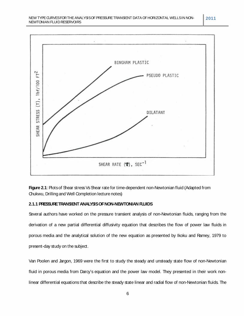
the changes in the shear rate and the constant of proportionality is called the plastic viscosity . Figure 2.1
from Chukwu, 2011 (Drilling and Well completion lecture notes) shows the difference in the relationship that
exists between shear stress and strain for the different non-Newtonian fluids as discussed above.
NEW TYPE CURVES FOR THE ANALYSIS OF PRESSURE TRANSIENT DATA OF HORIZONTAL WELLS IN NON-NEWTONIAN FLUID RESERVOIRS 2011
6
Figure 2.1: Plots of Shear stress Vs Shear rate for time-dependent non-Newtonian fluid (Adapted from Chukwu, Drilling and Well Completion lecture notes)
2.1.1 PRESSURE TRANSIENT ANALYSIS OF NON-NEWTONIAN FLUIDS
Several authors have worked on the pressure transient analysis of non-Newtonian fluids, ranging from the
derivation of a new partial differential diffusivity equation that describes the flow of power law fluids in
porous media and the analytical solution of the new equation as presented by Ikoku and Ramey, 1979 to
present-day study on the subject.
Van Poolen and Jargon, 1969 were the first to study the steady and unsteady state flow of non-Newtonian
fluid in porous media from Darcy’s equation and the power law model. They presented in their work non-
linear differential equations that describe the steady state linear and radial flow of non-Newtonian fluids. The
NEW TYPE CURVES FOR THE ANALYSIS OF PRESSURE TRANSIENT DATA OF HORIZONTAL WELLS IN NON-NEWTONIAN FLUID RESERVOIRS 2011
7
equations where solved numerically using the finite difference approach. The finite difference solution where
presented as plots of dimensionless wellbore pressure against dimensionless time. In considering unsteady
state flow for non-Newtonian fluids through porous media, Van Poolen and Jargon, 1969 described the flow of
a slightly compressible fluid through porous media by the equation below;
= ……………………………………………………………………………………………………………………………..……2.4
Equation 2.4 was solved using finite difference approach; dividing the model into number of grid cells and
solve number of simultaneous equation as obtained for each grid cell from equation 2.4 using initial and
boundary conditions as stated below;
Initial condition;
( , 0) = 0 …………………………………………………………………….…………………………………………………….………….………2.5
Boundary Condition at the wellbore;
= …………………………………………………………………………………………………………………………………………………2.6
Boundary condition at radius of drainage;
( , ) = 0 ……………………………………………………………………………………………………………………………………………..2.7
Van Poolen and Jargon considered drawdown and falloff response of non-Newtonian fluid in porous media.
They established a relationship between pressure differential and flow rate for a steady state flow. Their study
lacked analytical methodology and was only for vertical wells; the study considered one dimensional flow and
did not use the dimensionless log-log plot to analyze pressure data.
Consequently, the analysis of non-Newtonian injection Pressure data was studied by Ikoku and Ramey, 1979.
From the Blake-Kozeny equation as shown in equation 2.8, the power law non-Newtonian model and Darcy
NEW TYPE CURVES FOR THE ANALYSIS OF PRESSURE TRANSIENT DATA OF HORIZONTAL WELLS IN NON-NEWTONIAN FLUID RESERVOIRS 2011
8
equation they derived a new non-linear partial differential equation that described the flow of non-Newtonian
fluid in porous media.
= ( ) …………………………………………………………………………………………………………………………………..………2.8
In deriving their model for flow of non-Newtonian fluids through porous media, Ikoku and Ramey, 1979
assumed; radial flow, an isotropic reservoir of constant thickness, negligible compressibility, effects of gravity
where ignored, the reservoir fluid was a pseudo plastic fluid described by the power law model. In their work,
the law of conservation of mass, Darcy law and equation of sate where used to derive the new equation. The
dimensionless diffusivity equation that describes the radial flow of non-Newtonian fluid in porous media as
obtained by Ikoku and Ramey is as shown in equation 9 below;
+ = ……………………………………………………………………………………………………………..2.9
Equation 2.9 was solved analytically in the works of Ikoku and Ramey, 1979 in the Laplace domain. The
inversion of the resulting Laplacian solution was obtained numerically. In their work a more interpretative
method was applied because the slope of the straight-line section of the log-log plot of dimensionless pressure
against dimensionless time for different n values is very close. This might make type curve matching erroneous
when skin effect is considered. In the works of Ikoku and Ramey, a log-log plot of against gives a
straight line from which the flow index was obtained, the intercept at = 1 was also used to determine the
effective mobility provided is known. Furthermore, Ikoku and Ramey, 1979 proffered a method of
calculating skin from the log-log plot of against as well as the determination of the radius of
investigation from the steady state solution of equation 2.9. The study of Ikoku and Ramey, 1979 focused only
on the analysis of pressure transient data to obtain mobility, radius of investigation and skin. The study
considered one dimensional radial flow pressure transient in vertical wells and did not consider wellbore
storage.
NEW TYPE CURVES FOR THE ANALYSIS OF PRESSURE TRANSIENT DATA OF HORIZONTAL WELLS IN NON-NEWTONIAN FLUID RESERVOIRS 2011
9
Furthermore, Ikoku, 1980 extended well test analysis of non-Newtonian fluids to non-Newtonian injection
falloff testing. In his work the principle of superposition was used alongside the analytical solution of equation
2.9 to obtain the effective mobility ratio, reservoir permeability and skin factor. The validity of Ikoku, 1980
work was based on the assumption that the reservoir is liquid filled and the mobility of the injected fluid is
essential equal to the mobility of the in-situ fluid. Like previous works Ikoku, 1980 only focused on one
dimensional radial flow of non-Newtonian fluid as it applies to vertical wells.
Odeh and Yang, 1979 in their work derived a partial differential equation that describes the flow of non-
Newtonian , power law slightly compressible fluids in porous media, the equation was solved and the
unsteady state analytical solution was use to formulate a method for analyzing injection test data. The steady
state solution was used to analyze isochronal test data which was used to calculate the transient drainage
radius. The equation derived by Odeh and yang, 1979 is as shown below;
+ = ……………………………………………………………………………………………………………..…2.10
Their results was applied to four fields where injection operations is been carried out, in their work, the error
associated with the calculation of reservoir permeability from pressure transient analysis based on a
Newtonian fluid assumption was considered as compared to when the non-Newtonian pressure transient
analysis was made. Odeh and Yang, 1979 used a trial and error method to obtain the flow index ., they also
calculated permeability by a steady-state-type equation using the concept of equivalent transient drainage
radius. Odeh and Yang, 1979 found out that the methods of analysis accepted for Newtonian fluids are not
satisfactory for non-Newtonian fluids. Odeh and Yang’s work like that of Ikoku and Ramey, 1978 focused on
one dimensional radial pressure transient of non-Newtonian fluid in vertical wells
Ikoku and Ramey, 1980 considered the effect of skin and wellbore storage on the transient flow of non-
Newtonian fluids in petroleum reservoirs, a numerical wellbore storage simulator was used in their study of
NEW TYPE CURVES FOR THE ANALYSIS OF PRESSURE TRANSIENT DATA OF HORIZONTAL WELLS IN NON-NEWTONIAN FLUID RESERVOIRS 2011
10
skin and wellbore storage during the transient flow of power-law fluids in infinitely large and finite circular
reservoirs. Type- curve matching was used to analyze short-time well test data. They obtained a new
expression valid for wellbore storage effect when skin exist for infinitely large reservoirs and not for finite
circular reservoirs with no-flow or constant-pressure outer boundary. They derived a new expression for skin
factor and effective well radius for power-law flow. Equation 9 was solved using the no-flow outer boundary
and initial boundary conditions as stated below;
( , 0) = 0 ……………………………………………………………………………………………………………………………………….…2.11
1 > 0 ……………………………………………………………………………………………………………2.12
= 0 ……………………………………………………………………………………………………………….2.13
Where;
= ……………………………………………………………………………………………………………………………2.14
= …………………………………………………………………………………………………………………………..…………………….…2.15
= ….....................................................................................................................................................2.16
= …………………………………………………………………………………………………………………………………..……2.17
= ……………………………………………………………………………………………………………………………2.18
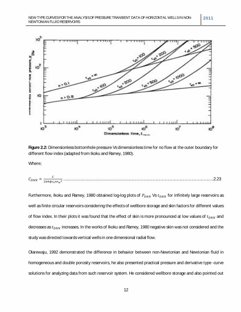
Equation 2.9 was solved in Laplace domain the works of Ikoku and Ramey, 1980 using the boundary conditions
as stated in equations 2.11 to 2.13. The plots of the dimensionless pressure versus the dimensionless time as
NEW TYPE CURVES FOR THE ANALYSIS OF PRESSURE TRANSIENT DATA OF HORIZONTAL WELLS IN NON-NEWTONIAN FLUID RESERVOIRS 2011
11
obtained in the works of Ikoku and Ramey, 1980 for a no flow outer boundary condition is as shown in the
figure below;
From figure 2.2 in the works of Ikoku and Ramey, it was noticed that at very high values of , curves of
different values of n tend to merge into a straight line of unit slope. In addition, Ikoku and Ramey, 1980
considered the effect of skin on pressure drop in the pressure transient of power-law fluid as shown in the
expression below;
= ………………………………………………………………………………………………………………………….…2.19
According to Ikoku and Ramey, 1979 the pressure drop due to skin can be also be calculated using the
expression;
= 1 . ( ) ……………………………………………………………………………………..…2.20
Thus
= 1 1 …………………………………………………………………………………………………….………2.21
In considering the effect of wellbore storage, Ikoku and Ramey, 1980 used a material balance concept that the
production rate must equal the rate of fluid withdrawal from the formation. For injection, the well injection
rate must equal the rate of storage of fluid in the wellbore plus the rate of entry into the formation. In
dimensionless terms, the wellbore storage is as defined in the works of Ikoku and Ramey below;
+ = 1 …………………………………………………………………………………………………2.22
NEW TYPE CURVES FOR THE ANALYSIS OF PRESSURE TRANSIENT DATA OF HORIZONTAL WELLS IN NON-NEWTONIAN FLUID RESERVOIRS 2011
12
Figure 2.2: Dimensionless bottomhole pressure Vs dimensionless time for no flow at the outer boundary for different flow index (adapted from Ikoku and Ramey, 1980).
Where;
= ………………………………………………………………………………………………………………………………..….2.23
Furthermore, Ikoku and Ramey, 1980 obtained log-log plots of Vs for infinitely large reservoirs as
well as finite circular reservoirs considering the effects of wellbore storage and skin factors for different values
of flow index. In their plots it was found that the effect of skin is more pronounced at low values of and
decreases as increases. In the works of Ikoku and Ramey, 1980 negative skin was not considered and the
study was directed towards vertical wells in one dimensional radial flow.
Olarewaju, 1992 demonstrated the difference in behavior between non-Newtonian and Newtonian fluid in
homogeneous and double porosity reservoirs, he also presented practical pressure and derivative type -curve
solutions for analyzing data from such reservoir system. He considered wellbore storage and also pointed out
NEW TYPE CURVES FOR THE ANALYSIS OF PRESSURE TRANSIENT DATA OF HORIZONTAL WELLS IN NON-NEWTONIAN FLUID RESERVOIRS 2011
13
that the rise in pressure decreases with increase in n, In obtaining the type curves for non-Newtonian fluids
when wellbore storage is considered, Olarewaju, 1992 presented that derivative type curves for non-
Newtonian fluids do not converge to a horizontal 0.5 line as generally noticed for Newtonian flow type curves
when wellbore storage is considered. It was also noted in his work that the semi-log straight line that exist
beyond the radial flow in the characteristic semi-log existing for Newtonian fluids is not present
for non-Newtonian fluids, rather a semi-log curve exist. A practical example was made in his study to show
how the type curves developed can be used to calculate mobility and reservoir permeability for a given
effective viscosity and porosity. Olarewaju, 1992 concluded in his work that the conventional semi-log analysis
cannot be used if the fluid flowing in the reservoir is non-Newtonian. Although he was able to develop type
curves for the analysis pressure transient of non-Newtonian fluids as well as show the misinterpretation that
could arise in using a Newtonian type curves to analyze pressure transient of non-Newtonian fluids, His study
was only directed to vertical wells alone and in one dimensional radial flow.
In the study of Katime-Meindl and Tiab, 2001, they presented an interpretation technique for pressure
behavior of non-Newtonian fluids flow in a homogeneous reservoir without the use of type-curve matching
with the aid of the Tiab’s direct synthesis technique considering no-flow and constant pressure boundary
conditions. In their study a step by step approach for obtaining mobility, wellbore storage coefficient, skin
factor and the distance to the nearest boundary without type-curve matching was introduced. Katime-Meindl
and Tiab, 2001 study was based on the assumption made in Ikoku and Ramey, 1979 study. The Stehfest
algorithm was used to invert the Laplace domain solution that incorporated skin and wellbore storage. Several
derivative type-curve where developed for different wellbore storage and skin for various flow indexes in their
work. In the study a new equation that is similar to the generally known wellbore storage equation which is in
terms of was obtained.
NEW TYPE CURVES FOR THE ANALYSIS OF PRESSURE TRANSIENT DATA OF HORIZONTAL WELLS IN NON-NEWTONIAN FLUID RESERVOIRS 2011
14
An equation was also obtained in their work to estimate the starting time of the infinite acting line of the
pressure derivative dimensionless plot for different n values which was in agreement with the values obtained
in the works of Ikoku and ramey, 1979. Furthermore, they proffered techniques of obtaining the mobility ratio
when the infinite acting radial line is not obvious or when there is noise in the pressure derivative data,
Katime-Meindl and Tiab, 2001 also presented method of calculating the distance to the boundary as well. An
example was made on a vertical well in Katime-Meindl and Tiab, 2001 to validate the study. The study did not
consider the pressure transient analysis of non-Newtonian fluids in horizontal well.
More recently, Igbokoyi and Tiab, 2007 obtained new type curves for the analysis of pressure transient data
dominated by skin and wellbore storage as applied to non-Newtonian fluids. In their comprehensive work, the
Laplace domain solution of Ikoku and Ramey, 1979 formed the Mathematical basis of their model. Their type-
curve did not use the dimensionless grouping of skin factor and wellbore storage as used in Bourdet and
Gringarten, 1980. In their work, they grouped the dimensionless wellbore storage with dimensionless time.
The log-log pressure derivative plots at the infinite acting radial flow for the non-Newtonian fluids of various
indexes intersected the Newtonian infinite acting pressure derivative line at = 1 which formed a fulcrum
point for type-curve matching. In addition the Tiab direct synthesis technique was also applied in the
evaluation of non-Newtonian well test data in non-Newtoniann fluid flow which did not involve any type-curve
matching. An infinite acting behavior was also assumed. The analytical solution in their work was similar to
that of Ikoku and Ramey, 1979. Stehfest algorithm was used to invert the solution obtained in the Laplace
domain. Igbokoyi and Tiab, 2007 obtained pressure derivative plots for different skin for various flow indexes.
Skin factor, dimensionless wellbore storage and mobility where estimated by type curve matching in their
study. The Tiab direct synthesis technique was applied based on the unique intersection of the characteristic
line on the log-log plot of the type-curve developed. The step in the TDS technique was used to obtain
expression to calculate permeability, skin, mobility ratio and wellbore storage. Igbokoyi and Tiab, 2007
NEW TYPE CURVES FOR THE ANALYSIS OF PRESSURE TRANSIENT DATA OF HORIZONTAL WELLS IN NON-NEWTONIAN FLUID RESERVOIRS 2011
15
validated their study by applying it to a case when n=1 found in Lee, 1982 using the type-curve matching
approach, TDS and the conventional method. It was found out in their study that the results obtained from the
TDS and that for the conventional method for the long time section was higher. Although the works of
Igbokoyi and Tiab was quite comprehensive it fails to address horizontal well test analysis of non-Newtonian
fluids.
Vongvuthipornchai and Raghavan, 1987 studied the pressure falloff behavior for non-Newtonian power law
fluids in vertically fractured wells after injection. In their study they considered wells intercepting infinite-
conductivity and uniform flux fractures, the procedures for identifying the flow regimes was also considered in
the study. In addition, Vongvuthipornchai and Raghavan, 1987 considered the falloff pressure response of
unfractured wells by also examining the validity of using the superposition principle to analyze pressure falloff
data provided the pseudo radial flow does exist. They found out that there is the need for corrections in the
pressure transient expression obtained by Odeh and Yang, 1979 for a power law index n less than 0.6. The
methodology of this present study is similar to the methodology of the study of Vongvuthipornchai and
Raghavan, 1987. The underlying assumptions and mathematical model used in Vongvuthipornchai and
Raghavan, 1987 work is similar to those used in the works of Murtha and Ertekin, 1983 and that of Ikoku and
Ramey, 1979. In their study skin region was incorporated by using the thick skin concept. In their analysis of
injection pressure response, they used the same equation as used in Ikoku and Ramey, 1979 to validate the
value on n by plotting Vs . The numerical solution of dimensionless pressure and slopes of Cartesian
plots was compared with the solution obtained by Odeh and yang, 1979 and the values were found to be
comparatively close. Furthermore, the influence of producing time on falloff data was also considered in their
study and this was used in the determination of n from the slope of the pressure response curve on log-log
plot. In the study of the effect of superposition in the analysis of falloff data they concluded that the direct
application of superposition principle in the analysis of falloff data can result in significant errors as the value
NEW TYPE CURVES FOR THE ANALYSIS OF PRESSURE TRANSIENT DATA OF HORIZONTAL WELLS IN NON-NEWTONIAN FLUID RESERVOIRS 2011
16
of n decreases, hence the need for a correction factor. It was also shown in the works of Vongvuthipornchai
and Raghavan, 1987 that shut-in responses follow the same curve irrespective of the injection time
provided that .
Vongvuthipornchai and Raghavan, 1987 validated their work with an example application to show the effect of
the correction factor. Vongvuthipornchai and Raghavan, 1987 finally considered both injection and falloff
pressure behavior of non-Newtonian fluids at fractured wells in analyzing fractured wells a methodology
which is applied in this study a new definition of dimensionless time was formulated based on the fracture
half-length, which was given by;
= …………………………………………………………………………………………………………………………………………2.24
Where is given by
= …………………………………………………………………………………………………………………………..……….2.25
It should be noted that used in the works of Vongvuthipornchai and Raghavan, 1987 is the same as
used in the works of Ikoku and Ramey, 1979, also the definition of the dimensionless pressure is as written
below;
= ( )
………………………………………………………………………………………………………………………………2.26
The Pressure response was studied for both infinite conductivity and uniform flux fracture. According to the
study, Infinite conductivity solution is useful if the well is hydraulically fractured and if the fracture length is
small, generally infinite conductivity is classified if the dimensionless fracture conductivity is greater and equal
to 500. Uniform flux solution were proposed to be useful in situations where wells are stimulated by acid
fracturing or where wells are inadvertently fractured by high injection pressures. Their computations indicated
NEW TYPE CURVES FOR THE ANALYSIS OF PRESSURE TRANSIENT DATA OF HORIZONTAL WELLS IN NON-NEWTONIAN FLUID RESERVOIRS 2011
17
that at early times a well-defined straight line with slope equal to 0.5 on the log-log coordinates will be
evident, they concluded that is given by;
= …………………………………………………………………………………………………………..……………………………..2.27
Furthermore, Vongvuthipornchai and Raghavan, 1987 used pressure derivative technique to analyze the
response of a well intercepting a planar fracture during the injection of a non-Newtonian power-law fluid. In
order to achieve type-curve matching a correlation was formulated for convenient analysis of falloff data. The
analysis of pressure behavior at wells intercepting uniform-flux was similar of those of infinite-conductivity in
the study of Vongvuthipornchai and Raghavan, 1987. Similarly a simultaneous match of Pressure and Pressure
derivative log-log plots were used to improve matching. Vongvuthipornchai and Raghavan, 1987, the partial
linear coordinate differential equation that governs the transient flow of a non-Newtonian and slightly
compressible liquid for vertically fractured well in a closed cube reservoir model is as shown in equation 2.28
below. The works of Vongvuthipornchai and Raghavan, 1987 did not consider the pressure transient of non-
Newtonian fluids in Horizontal wells and only considered 2 dimensional flows.
+ = ………………………………………………………………………………………………………..2.28
Where is the dimensionless pressure at any point in the reservoir and( , ), , are the
dimensionless distance based on Lxf ( the length of the fracture)
( , , ) = [ ( , , ) ]……………………………………………………………………………………………………2.29
= …………………………………………………………………………………………………………………………………………….………2.30
= ……………………………………………………………………………………………………………………………………………..…...2.31
NEW TYPE CURVES FOR THE ANALYSIS OF PRESSURE TRANSIENT DATA OF HORIZONTAL WELLS IN NON-NEWTONIAN FLUID RESERVOIRS 2011
18
Both Infinite conductivity and uniform flux were assumed in the study, for infinite conductivity the wellbore
boundary condition for injection at a constant rate was given by;
………………………………………………………………………………………………………………………2.32
And
1, = 0, = ( )………………………………………………………………………………………………….2.33
For the uniform flux idealization, Vongvuthipornchai and Raghavan, 1987 assumes that the flux is uniform on
the fracture surface ( 1, = 0) . In this case equation 46 was not valid; i.e., the pressure along the
fracture surface is a variable and = 0,0, initial condition is given by;
1, = 0, = ( )……………………………………………………………………………………………………2.34
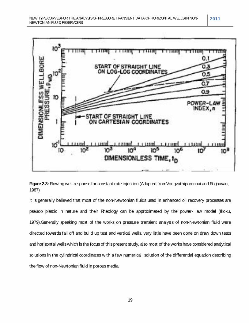
A log-log plot of Vs showing the flowing well response as obtained by Vongvuthipornchai and
Raghavan, 1987 for constant rate injection is as shown in the figure below;
NEW TYPE CURVES FOR THE ANALYSIS OF PRESSURE TRANSIENT DATA OF HORIZONTAL WELLS IN NON-NEWTONIAN FLUID RESERVOIRS 2011
19
Figure 2.3: Flowing well response for constant rate injection (Adapted fromVongvuthipornchai and Raghavan, 1987)
It is generally believed that most of the non-Newtonian fluids used in enhanced oil recovery processes are
pseudo plastic in nature and their Rheology can be approximated by the power- law model (Ikoku,
1979).Generally speaking most of the works on pressure transient analysis of non-Newtonian fluid were
directed towards fall off and build up test and vertical wells, very little have been done on draw down tests
and horizontal wells which is the focus of this present study, also most of the works have considered analytical
solutions in the cylindrical coordinates with a few numerical solution of the differential equation describing
the flow of non-Newtonian fluid in porous media.
NEW TYPE CURVES FOR THE ANALYSIS OF PRESSURE TRANSIENT DATA OF HORIZONTAL WELLS IN NON-NEWTONIAN FLUID RESERVOIRS 2011
20
2.2 HORIZONTAL WELLS
Horizontal wells accelerate recovery and hence improve economics in a broad range of reservoir
characteristics (Medeiros et al, 2007 IPTC11781). Horizontal wells can greatly increase the contact area of the
wellbore and the pay zone; so they are commonly applied in reservoirs to enhance the production and
recovery, especially in low permeability formations (Al Rbeawi and Tiab, 2011, SPE 142316). They also have
been used successfully: (a) to intersect fractures and effectively drain reservoirs; (b) in water and gas driven
reservoirs to minimize water and gas coning ; (c) in both high and low producing reservoirs to reduce the
number of producing wells; (d) in tertiary recovery application to enhance the contact between the well and
the reservoir, and (e) finally in offshore reservoirs as well as in environmentally sensitive areas to cut down
the cost of drilling and the number of production facilities (Al Rbeawi and Tiab, 2011, SPE 142316). These
advantages of horizontal wells have made it widely applicable in the petroleum industry over the past few
decades. Amongst other applications, Horizontal wells are used in Enhanced oil recovery processes such as
steam injection; steam Assisted Gravity Drainage (SAGD), cyclic injection production techniques and
production of tight formations.
2.2.1 HORIZONTAL WELL PRESSURE TRANSIENT ANALYSIS
According to Rbeawi and Tiab, 2011(SPE 142316), five flow regimes have been observed for regular length
horizontal wells; early radial flow, early linear flow, pseudo radial flow, channel flow or late linear flow and
pseudo-steady state flow. While only four flow regimes have been observed for the extra-long well; linear
flow, pseudo-radial flow, channel flow, and pseudo-steady state flow or boundary affected flow. In most cases
all these flow regimes are not seen, for example the early radial flow might not be seen if it is obscured by
wellbore storage effects or near well-bore effects. Similarly, the pseudo steady state or boundary effect flow is
noticed if the draw down test is run for a long time. There are two types of pressure transient behavior
depending on effective dimensionless drain hole half-length, . If LD<10, flow is characterized by an initial
NEW TYPE CURVES FOR THE ANALYSIS OF PRESSURE TRANSIENT DATA OF HORIZONTAL WELLS IN NON-NEWTONIAN FLUID RESERVOIRS 2011
21
radial flow perpendicular to the drain hole axis followed by a transition to a pseudo- radial flow period. If
LD>10, the initial radial flow period ends instantaneously for all practical purposes. Flow is then characterized
by early time linear flow followed by a transition to late time pseudo-radial flow (Molts and Ramey, 1966). It
has also been established in the literature that the pressure response of drain hole or horizontal wells is
similar to those of vertical fractures, hence sometimes horizontal well are model as fractures. For cases where
LD>10, the uniform flux drain hole solution matches the uniform flux vertical fracture solution. From the
definition of LD, the similarity between drain holes and vertical fractures is directly proportional to the ratios
and and . (Molts and Ramey, 1966). Pressure derivative plots i.e. plots of logarithm of dimensionless
pressure derivative against logarithm of dimensionless time usually serve as a reliable means of analyzing
pressure transient of horizontal wells.
Pressure transient response was obtained by using the initial and boundary conditions in the works of Babu
and Odeh (1988). In the study, pressure drop were obtained at an arbitrary point (x,y,z) in the reservoir by
integrations of appropriate Green’s functions. In the work of Issaka and Ambastha (1992) the equation as
obtained in Babu and Odeh ‘s study was solved numerically using the Simpson’s rule for space integration and
trapezoidal rule for the time integration.
Most studies have considered horizontal well pressure transient analysis for Newtonian fluids while there have
been no study on the pressure transient analysis of non-Newtonian fluids in horizontal wells. This study seeks
to address this problem.
2.3 MATHEMATICAL MODELING AND SOLUTIONS
The Mathematical modeling of the diffusivity equation is based on the law of conservation of mass, the Darcy
equation and the equation state. The Importance of this non-linear differential equation has attracted
different types of solution ranging from analytical, numerical and semi-analytical solutions.
NEW TYPE CURVES FOR THE ANALYSIS OF PRESSURE TRANSIENT DATA OF HORIZONTAL WELLS IN NON-NEWTONIAN FLUID RESERVOIRS 2011
22
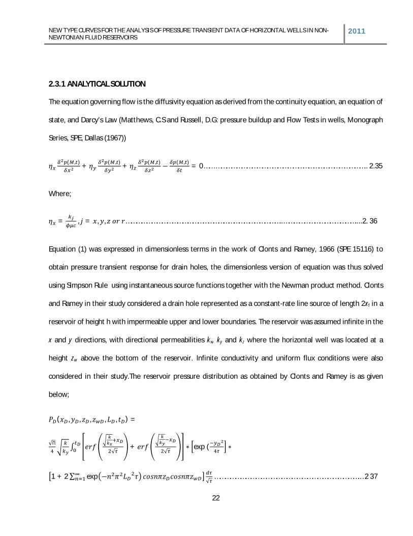
2.3.1 ANALYTICAL SOLUTION
The equation governing flow is the diffusivity equation as derived from the continuity equation, an equation of
state, and Darcy’s Law (Matthews, C.S and Russell, D.G: pressure buildup and Flow Tests in wells, Monograph
Series, SPE, Dallas (1967))
( , ) + ( , ) + ( , ) ( , ) = 0…… …………………………………………………………………………….. 2.35
Where;
= , = , , ………………………………………………………………………………..……………………………………....2. 36
Equation (1) was expressed in dimensionless terms in the work of Clonts and Ramey, 1966 (SPE 15116) to
obtain pressure transient response for drain holes, the dimensionless version of equation was thus solved
using Simpson Rule using instantaneous source functions together with the Newman product method. Clonts
and Ramey in their study considered a drain hole represented as a constant-rate line source of length 2xf in a
reservoir of height h with impermeable upper and lower boundaries. The reservoir was assumed infinite in the
x and y directions, with directional permeabilities kx, ky and kz where the horizontal well was located at a
height zw above the bottom of the reservoir. Infinite conductivity and uniform flux conditions were also
considered in their study.The reservoir pressure distribution as obtained by Clonts and Ramey is as given
below;
( , , , , , ) =
+ exp (
1 + 2 exp ………………………………………………………………………….…2 37
NEW TYPE CURVES FOR THE ANALYSIS OF PRESSURE TRANSIENT DATA OF HORIZONTAL WELLS IN NON-NEWTONIAN FLUID RESERVOIRS 2011
23
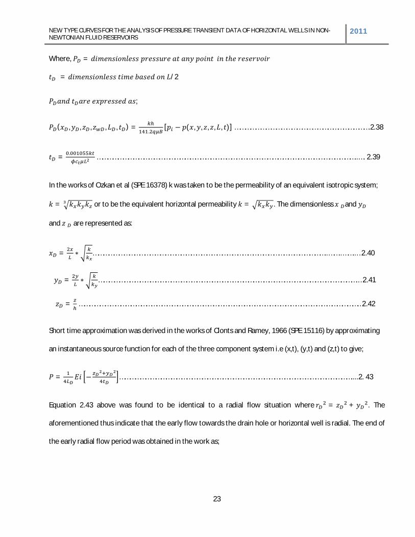
Where, =
= /2
;
( , , , , , ) =.
[ ( , , , , , )] …………………………………………………………………….2.38
= . ……………………………………………………………………………………………………………………………………..…. 2.39
In the works of Ozkan et al (SPE 16378) k was taken to be the permeability of an equivalent isotropic system;
= or to be the equivalent horizontal permeability = . The dimensionless and
and are represented as:
= ………………………………………………………………………………………………………………………..……..……..…2.40
= …………………………………………………………………………………………………………………………………….…2.41
= …………………………………………………………………………………………………………………………………………………2.42
Short time approximation was derived in the works of Clonts and Ramey, 1966 (SPE 15116) by approximating
an instantaneous source function for each of the three component system i.e (x,t), (y,t) and (z,t) to give;
= ………………………………………………………………………………………………………………………....2. 43
Equation 2.43 above was found to be identical to a radial flow situation where = + . The
aforementioned thus indicate that the early flow towards the drain hole or horizontal well is radial. The end of
the early radial flow period was obtained in the work as;
NEW TYPE CURVES FOR THE ANALYSIS OF PRESSURE TRANSIENT DATA OF HORIZONTAL WELLS IN NON-NEWTONIAN FLUID RESERVOIRS 2011
24
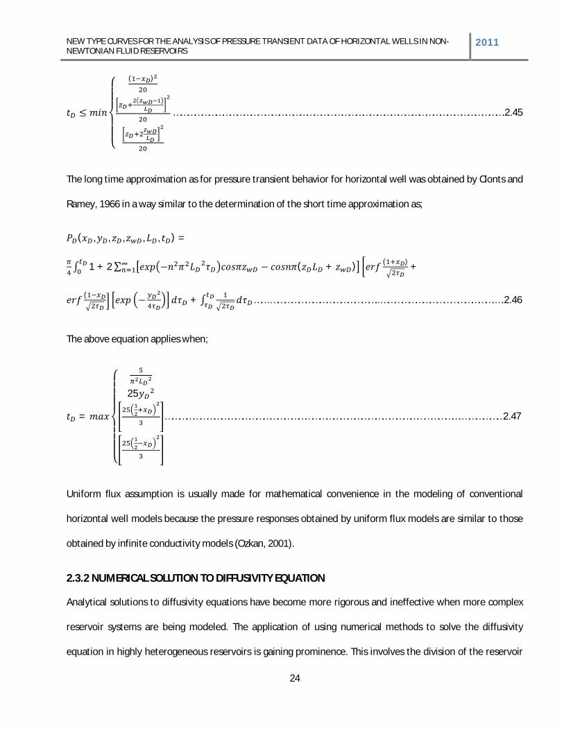
( )
…………………………………………………………………………………………………………………………….2.45
The long time approximation as for pressure transient behavior for horizontal well was obtained by Clonts and
Ramey, 1966 in a way similar to the determination of the short time approximation as;
( , , , , , ) =
1 + 2 ( + ) ( ) +
( + …… ………………………………………..………………………………………….….2.46
The above equation applies when;
=
25
……………………………………………………………………………………………………………….………………2.47
Uniform flux assumption is usually made for mathematical convenience in the modeling of conventional
horizontal well models because the pressure responses obtained by uniform flux models are similar to those
obtained by infinite conductivity models (Ozkan, 2001).
2.3.2 NUMERICAL SOLUTION TO DIFFUSIVITY EQUATION
Analytical solutions to diffusivity equations have become more rigorous and ineffective when more complex
reservoir systems are being modeled. The application of using numerical methods to solve the diffusivity
equation in highly heterogeneous reservoirs is gaining prominence. This involves the division of the reservoir
NEW TYPE CURVES FOR THE ANALYSIS OF PRESSURE TRANSIENT DATA OF HORIZONTAL WELLS IN NON-NEWTONIAN FLUID RESERVOIRS 2011
25
into fine grids and the use of very small time steps. In most cases tools like finite difference, finite volume,
Boundary element and finite element methods are used to convert the diffusivity Partial differential equations
into linear systems of equations, this process is called Discretization. Of all these numerical methods the finite
difference numerical solution to partial differential equation is widely used because of its simplicity. This work
involves the application of finite difference approach to solve the modeled non-Newtonian diffusivity
equation.
2.3.3 FINITE DIFFERENCE APPROXIMATION
Finite difference is a numerical tool used to solving Ordinary and Partial differential equations, especially non-
linear differential equations. In petroleum engineering, finite difference is used to solve partial differential
equation that describes the flow of fluid in porous media i.e. the diffusivity equation. The finite-difference
method is implemented by superimposing a finite-difference grid over the reservoir to be modeled. The
chosen grid system is then used to approximate the spatial derivatives in the continuous equations. These
approximations are obtained by truncating the Taylor series expansion of the unknown variable Ertekin et al ,
2001
The Block centered scheme which is defined by the centers of each grid block and the point distributed finite-
difference schemes defined by the distribution of grid points over the reservoir before boundaries are
specified are the widely used in reservoir simulation applicable to the spherical, cylindrical, elliptical and linear
or rectangular coordinate system. The rectangular coordinate system is commonly used in reservoir simulation
such as predicting well performance and to model pattern element in pattern flooding. The block centered
system is commonly used because the volume associated with each grid point is clearly defined; it also
adheres more closely to the material balance concept of reservoir engineering. Through discretization a
system of equations can be obtained to compute the unknown properties such as pressure or saturation for
every grid cell that the reservoir has been divided into. Furthermore, differential equations can be digitized
NEW TYPE CURVES FOR THE ANALYSIS OF PRESSURE TRANSIENT DATA OF HORIZONTAL WELLS IN NON-NEWTONIAN FLUID RESERVOIRS 2011
26
using the central difference, forward difference or the backward difference approximations. The central
difference approximation is used for the second derivative in the diffusivity equation because of its higher
order of approximation;
= …………………………………………………………………………………….………………………………………..…….2.48
The first order derivative is usually approximated by the backward difference approximation as shown below;
= ………………………………………………………………………………..………………………………………………………….….2.49
The choice of the finite difference approximation to used is dependent on the stability of the systems of
equations obtained. Stability is a property that describes the capacity of a small error to propagate and grow
with subsequent calculations Ertekin et al , 2001. The grid system is used to divide the reservoir into small
partitions which will have the characteristic properties assigned. In most cases, finer grids are used for
important features such as the producing zones while larger size grids may be used for aquifers and less
important features. Boundary conditions are implemented in two ways; firstly, when there are no discrete
points at the boundary which is in most cases used for no flow boundaries while the other method is
applicable when points are specified on the boundary. The grids are distributed over the entire reservoir.
2.3.4 FINITE DIFFERENCE FORMULATION
If the flow of fluid through one dimensional system, say a 1D grid block is described by a second order
differential equation as shown below in Ertekin et al, 2001;
…………………………………………………………………2.50
This can be further re-written as;
NEW TYPE CURVES FOR THE ANALYSIS OF PRESSURE TRANSIENT DATA OF HORIZONTAL WELLS IN NON-NEWTONIAN FLUID RESERVOIRS 2011
27
+ = ……………………………………….……2.51
The use of central difference to approximate gives
= = ………………………………………………………………………………………………………………..………2.52
= = …………………………………………………………………….………………………………………….………2.53
Equation 2.51 thus becomes;
( ) ( ) + = ( )…………………………2.54
Although the central -difference approximation is a higher order approximation, it is generally not used
because of stability problems and difficulties in applying the initial conditions Aziz and Settari, 1990. Like with
when approximating finite difference for special derivative, the forward and backward finite difference is used
for first order time derivative while the second central difference approximation is used for second order time
derivative.For example, the backward - difference approximation for a first order derivative with respect to
time.
= ……………………………………………………………………………………………………………………………………………2.55
While the forward difference approximation is given as;
= ……………………………………………………………………………………………………………………..………………...2.56
Although equation 2.55 and 2.56 looks similar the difference between them is that in the forward difference
approximation of the pressure derivative with respect to time, the right hand side derivative with respect to
NEW TYPE CURVES FOR THE ANALYSIS OF PRESSURE TRANSIENT DATA OF HORIZONTAL WELLS IN NON-NEWTONIAN FLUID RESERVOIRS 2011
28
space is approximated using a finite difference at time n, while the backward difference uses a derivative with
respect to space at time n+1. The central difference approximation with respect to time considers a base time
of n as shown in the equation below;
= ……………………………………………………………………………………………………………………………………………2.57
The two most common boundary conditions are the constant pressure boundary condition and the no-flow
boundary condition. A constant pressure boundary condition implies that the pressure gradient at the
reservoir boundary is constant as denoted by the equation below;
= = …………………………………………………………………………………………………………………………………….2.58
Where C is a constant which may be time dependent or not, it should be noted that the boundary condition
can be expressed as forward, backward or central difference as it was discussed for the time derivative
discretization. For a no flow boundary condition; C=0 in equation 2.58.
The explicit and implicit finite difference formulations are usually used to determine the pressure for each
time step. Because of the time levels assigned to the pressures on the left sides of the equations, forward –
difference equation results in an explicit calculation for the new –time-level pressures in the n+1 time basis
while the backward –difference equation results in an implicit calculation for the new-time-level pressures.
The next chapter will discuss more about the application of finite difference in this study.
2.4 CONVENTIONAL METHODS AND TYPE CURVES ANALYSIS OF PRESSURE TRANSIENT DATA
Over the years type curves have become an important tool in the analysis of well test data especially when
dealing with horizontal wells, with the aid of type curve matching as presented by Ramey, 1976 (SPE 5878).
Type curve matching has thus help on the evaluation of reservoir properties such as the permeabilities kx, ky
and kz as well as near well bore effects such as skin and wellbore storage. The LD match point yields the ratio
NEW TYPE CURVES FOR THE ANALYSIS OF PRESSURE TRANSIENT DATA OF HORIZONTAL WELLS IN NON-NEWTONIAN FLUID RESERVOIRS 2011
29
and the PD match point yield , the xD match point combined with other directional permeability data
yields the may be determined by the time match (Clonts and Ramey,1966). The skin factor is usually
determined by subtracting the pseudo skin factor determined just before the long time approximation from
the total skin factor. Skin factor is negative for a stimulated wellbore and positive for a damaged wellbore.
To use pressure derivatives in well test analysis, it is necessary to develop design equations and type curves
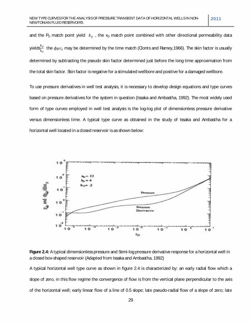
based on pressure derivatives for the system in question (Issaka and Ambastha, 1992). The most widely used
form of type curves employed in well test analysis is the log-log plot of dimensionless pressure derivative
versus dimensionless time. A typical type curve as obtained in the study of Issaka and Ambastha for a
horizontal well located in a closed reservoir is as shown below:
Figure 2.4: A typical dimensionless pressure and Semi-log pressure derivative response for a horizontal well in a closed box-shaped reservoir (Adapted from Issaka and Ambastha, 1992)
A typical horizontal well type curve as shown in figure 2.4 is characterized by: an early radial flow which a
slope of zero, in this flow regime the convergence of flow is from the vertical plane perpendicular to the axis
of the horizontal well; early linear flow of a line of 0.5 slope; late pseudo-radial flow of a slope of zero; late
NEW TYPE CURVES FOR THE ANALYSIS OF PRESSURE TRANSIENT DATA OF HORIZONTAL WELLS IN NON-NEWTONIAN FLUID RESERVOIRS 2011
30
linear flow represented by a straight line of slope of 0.5 and a pseudo-steady state flow characterized by a unit
slope.A conventional plot of Pwf against t in the early radial flow gives a straight line whose slope is as given;
= . …………………………………………………………………………………………………………………………………………….2.59
From equation 13 above the term can be easily obtained. In the works of Ozkan, 2001, for a long
horizontal well satisfying the criteria;
100 …………………………………………………………………………………………………………………………………………..2.60
The intermediate linear flow regime is obvious; a conventional Cartesian plot of Pwf against will give a
straight line with a slope of;
= . ……………………………………………………………………………………………….……………………………………2.61
From equation 2.61 above the permeability can be obtained
The pseudo-radial or late radial flow is thus characterized on a conventional Pwf against t plot as a straight line
with the slope;
= .
………………………………………………………………………………………………………………………………….2.62
From equation 2.62 above the term which is regarded as the horizontal permeability can be obtained.
From the afore mentioned procedure it could be seen that the conventional methods can only be used to
determine the horizontal permeability, ky and . However, It also be noted that type-curve matching
can only provide the horizontal permeability and the vertical permeability, thus a combination of
NEW TYPE CURVES FOR THE ANALYSIS OF PRESSURE TRANSIENT DATA OF HORIZONTAL WELLS IN NON-NEWTONIAN FLUID RESERVOIRS 2011
31
conventional and type curve pressure transient analysis will enable the permeabilities description of a
reservoir.
It should be noted that the analysis of horizontal well test data might be incomplete due to near wellbore
conditions such as wellbore storage and skin, restrictions caused by extremely long wells causing a delay in the
pseudo-radial flow and the non-existence of the intermediate linear or pseudo-radial flow.
2.4.1 WELLBORE STORAGE
As stated earlier, the presence of wellbore storage affects the pressure transient of horizontal wells. In the
analysis of the drawbacks of conventional pressure transient method, Ozkan (2001) showed that a moderate –
to-Small wellbore storage can destroy the early and intermediate –time flow periods. Unlike vertical wells, the
analysis of horizontal well pressure data after the wellbore storage effect cannot provide information about
the directional permeabilities obtainable without the influence of the wellbore storage. Techniques such as
advance convolution are used to remove the effect of well bore storage on horizontal well pressure transient
for the complete analysis of well test data.
According to Ikoku and Ramey, 1979 the physical effect of wellbore storage is to cause a sand-face injection or
production that initially is zero and increases toward the surface wellhead flow rate as a function of time, even
though the surface injection or production is held constant. From their work , they assumed fluid is stored in
the wellbore by virtue of compression, the wellbore storage constant C (m3/Pa) is defined by the material
balance;
= ………………………………………………………………………………………………………………………………………………………2.63
= + ………………………………………………………………………………………………………………………………..………2.64
NEW TYPE CURVES FOR THE ANALYSIS OF PRESSURE TRANSIENT DATA OF HORIZONTAL WELLS IN NON-NEWTONIAN FLUID RESERVOIRS 2011
32
2.4.2 SKIN FACTOR
The definition of Skin by Ozkan, 2001 considers the steady-state skin factor putting into consideration the
possible non-uniformity of the skin zone. The skin factor has been found to be a function of flux which is in
turn a function of time and location along the horizontal well length as seen from equation 2.70. The skin
factor obtained from equation 2.70 is thus time –dependent besides flow period when the flux remains
constant. According to Ozkan,2001, analysis of well test data are subjected to some error due to the presence
of non-uniform skin distribution, errors are minimal when shin distribution are regarded to be uniform. The
differences in the skin at the heel and at the toe of a horizontal well due to non-uniform skin distribution can
lead to erroneous determination of horizontal permeability. The presence of uniform or non-uniform skin also
masks the analysis of horizontal well test data. Therefore, the effect of skin factor should be incorporated into
the analytical solution of the pressure transient equation as presented by Ozkan and Raghavan, 1997 in the
equation below;
( , ) = ( , +, , ) + ( , ) ( )………………………………………………………………………….2.65
= ( , ) ………………………………………………………………………………………………………………………………….……...2.66
( ) = . ( , )
( , ) ……………………………………………………………………………………………………………………….…..2.67
=pressure drop across the skin zone.
Assuming that;
( ) = ( , ) ( )…………………………………………………………………………………………………..….……………2.68
( , ) = ( +, , ) + ( , ) (0, )………………………………………………………………………….2.69
= 1.151.
…..........................................................................................................................2.70

NEW TYPE CURVES FOR THE ANALYSIS OF PRESSURE TRANSIENT DATA OF HORIZONTAL WELLS IN NON-NEWTONIAN FLUID RESERVOIRS 2011
33
is the drawdown measured at the heel of the well at a given time t, Is the logarithmic derivative of the
drawdown with respect to time defined at the same time and Is the dimensionless pressure without skin
effect.
NEW TYPE CURVES FOR THE ANALYSIS OF PRESSURE TRANSIENT DATA OF HORIZONTAL WELLS IN NON-NEWTONIAN FLUID RESERVOIRS
2011
34
CHAPTER THREE
3.0 METHODOLOGY
The approach used in carrying out this study is as listed below;
Establishing basic assumptions
Modeling of Partial differential diffusivity equation that describes the flow of non-Newtonian
fluids based on the assumptions made. The modeling involved the use of the law of
conservation of mass, the Darcy equation and the equation of state from which the viscosity
ratio is obtained.
Expressing the diffusivity equations in terms of dimensionless terms using the appropriate
dimensionless variables.
Formulating initial and boundary conditions that would aid solution of the diffusivity
equation
Discretizing the diffusivity equation with the aid of finite difference approximation
Writing of a MATLAB code to solve the system of equations obtained from discretization. This
will help in obtaining dimensionless pressured for each time step.
Writing a MATLAB program for the convergence of the viscosity ratio
Making log-log plots of ( ) for
different well and reservoir configurations when Newtonian fluids are considered for
validation purpose.
Making log-log plots of ( ) for
different well and reservoir configurations and non-Newtonian reservoir fluids.
Developing type curves for non-Newtonian reservoir fluids with power law
index = 0.1 1.0 .

NEW TYPE CURVES FOR THE ANALYSIS OF PRESSURE TRANSIENT DATA OF HORIZONTAL WELLS IN NON-NEWTONIAN FLUID RESERVOIRS 2011
35
3.1 BASIC ASSUMPTIONS
The Basic assumptions made in the modeling of the problem are;
Isothermal, single-phase and slightly compressible fluid.
Linear fluid flow into the wellbore,
Steady state effective viscosity.
Homogeneous reservoir with an average porosity with permeability anisotropy.
Permeability differs with direction, kx, ky and kz taking kx to be the maximum
permeability
The Horizontal well was place in the direction perpendicular to the maximum
permeability ,that is along the y-coordinates
Power–law Model was used to describe the Non-Newtonian fluid.
Negligible effects of gravity.
Reservoir is of constant thickness
Pseudo-plastic fluid is being considered (0<n<1.0)
No flow reservoir boundary is assumed
The methodology used in this work is based on the one used in the works of Vongvuthipornchai and
Raghavan, 1987

NEW TYPE CURVES FOR THE ANALYSIS OF PRESSURE TRANSIENT DATA OF HORIZONTAL WELLS IN NON-NEWTONIAN FLUID RESERVOIRS 2011
36
3.2 MATHEMATICAL FORMULATION OR MODELING
Figure 3.1: Diagram showing the flow through a porous cuboid reservoir model
From the law of conservation of mass;
=
+ + = ( )
( ) ………………………………………………………………………………………………………………….3.1
=
= ( )
= (%)
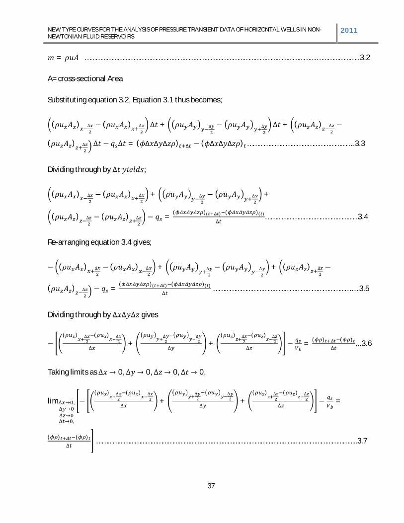
NEW TYPE CURVES FOR THE ANALYSIS OF PRESSURE TRANSIENT DATA OF HORIZONTAL WELLS IN NON-NEWTONIAN FLUID RESERVOIRS 2011
37
= ……………………………………………………………………………………………………………….……………………3.2
A= cross-sectional Area
Substituting equation 3.2, Equation 3.1 thus becomes;
( ) ( ) + + ( )
( ) = ( ) ( ) …………………………………………………..3.3
Dividing through by ;
( ) ( ) + +
( ) ( ) = ( )( ) ( )( )……………………………………………3.4
Re-arranging equation 3.4 gives;
( ) ( ) + + ( )
( ) = ( )( ) ( )( ) …………………………………………………………………..…3.5
Dividing through by gives
( ) ( )+ +
( ) ( )= ( ) ( ) ...3.6
Taking limits as 0, 0, 0, 0,
lim ,
,
( ) ( )+ +
( ) ( )=
( ) ( ) ……………………………………………………………………………………………………………………………..3.7
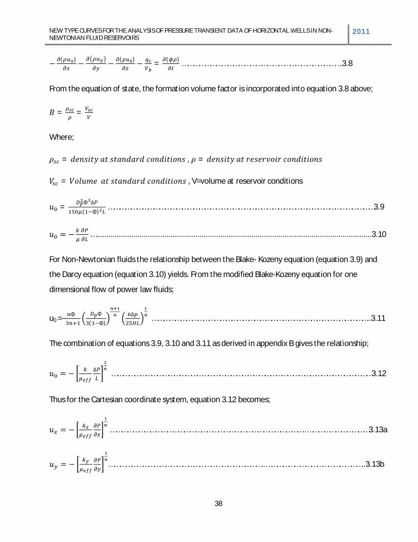
NEW TYPE CURVES FOR THE ANALYSIS OF PRESSURE TRANSIENT DATA OF HORIZONTAL WELLS IN NON-NEWTONIAN FLUID RESERVOIRS 2011
38
( ) ( ) = ( ) ………………………………………………………………………….3.8
From the equation of state, the formation volume factor is incorporated into equation 3.8 above;
= =
Where;
= , =
= , V=volume at reservoir conditions
=( )
……………………………………………………………………………………………………………………………3.9
….....................................................................................................................................3.10
For Non-Newtonian fluids the relationship between the Blake- Kozeny equation (equation 3.9) and
the Darcy equation (equation 3.10) yields. From the modified Blake-Kozeny equation for one
dimensional flow of power law fluids;
u0 = ( ) ……………………………………………………………………………………………………..3.11
The combination of equations 3.9, 3.10 and 3.11 as derived in appendix B gives the relationship;
…………………………………………………………………………………………………………………………3.12
Thus for the Cartesian coordinate system, equation 3.12 becomes;
…………………………………………………………………………………………..……………………………3.13a
………………………………………………………………………..……………………………………………..3.13b
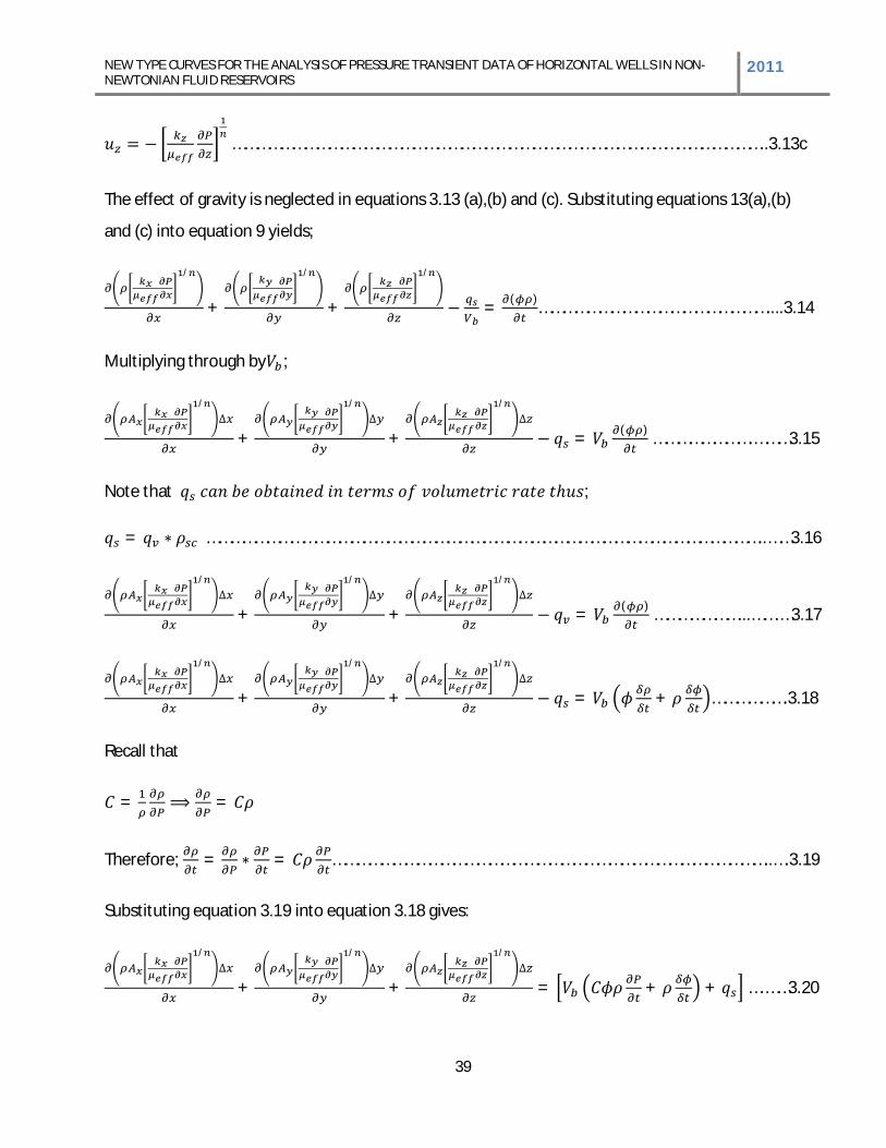
NEW TYPE CURVES FOR THE ANALYSIS OF PRESSURE TRANSIENT DATA OF HORIZONTAL WELLS IN NON-NEWTONIAN FLUID RESERVOIRS 2011
39
……………………………………………………………………………………………………………………..3.13c
The effect of gravity is neglected in equations 3.13 (a),(b) and (c). Substituting equations 13(a),(b)
and (c) into equation 9 yields;
/
+
/
+
/
= ( )…………………………………………………....3.14
Multiplying through by ;
/
+
/
+
/
= ( ) …………………….………3.15
Note that ;
= …………………………………………………………………………………………………………………………..……3.16
/
+
/
+
/
= ( ) …………………...…….…3.17
/
+
/
+
/
= + ……………….3.18
Recall that
= =
Therefore; = = ………………………………………………………………………………………………..….3.19
Substituting equation 3.19 into equation 3.18 gives:
/
+
/
+
/
= + + ….……3.20
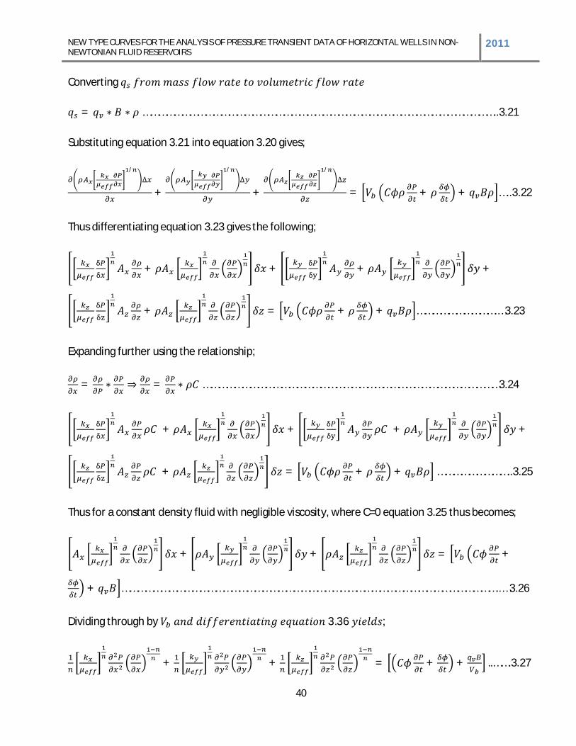
NEW TYPE CURVES FOR THE ANALYSIS OF PRESSURE TRANSIENT DATA OF HORIZONTAL WELLS IN NON-NEWTONIAN FLUID RESERVOIRS 2011
40
Converting
= ………………………………………………………………………………………………………………………..3.21
Substituting equation 3.21 into equation 3.20 gives;
/
+
/
+
/
= + + …..3.22
Thus differentiating equation 3.23 gives the following;
+ + + +
+ = + + ………………………….…3.23
Expanding further using the relationship;
= = ……………………………………………………………………………………………………3.24
+ + + +
+ = + + ………………………..3.25
Thus for a constant density fluid with negligible viscosity, where C=0 equation 3.25 thus becomes;
+ + = +
+ ………………………………………………………………………………………………………………………………..…3.26
Dividing through by 3.36 ;
+ + = + + ..…….3.27
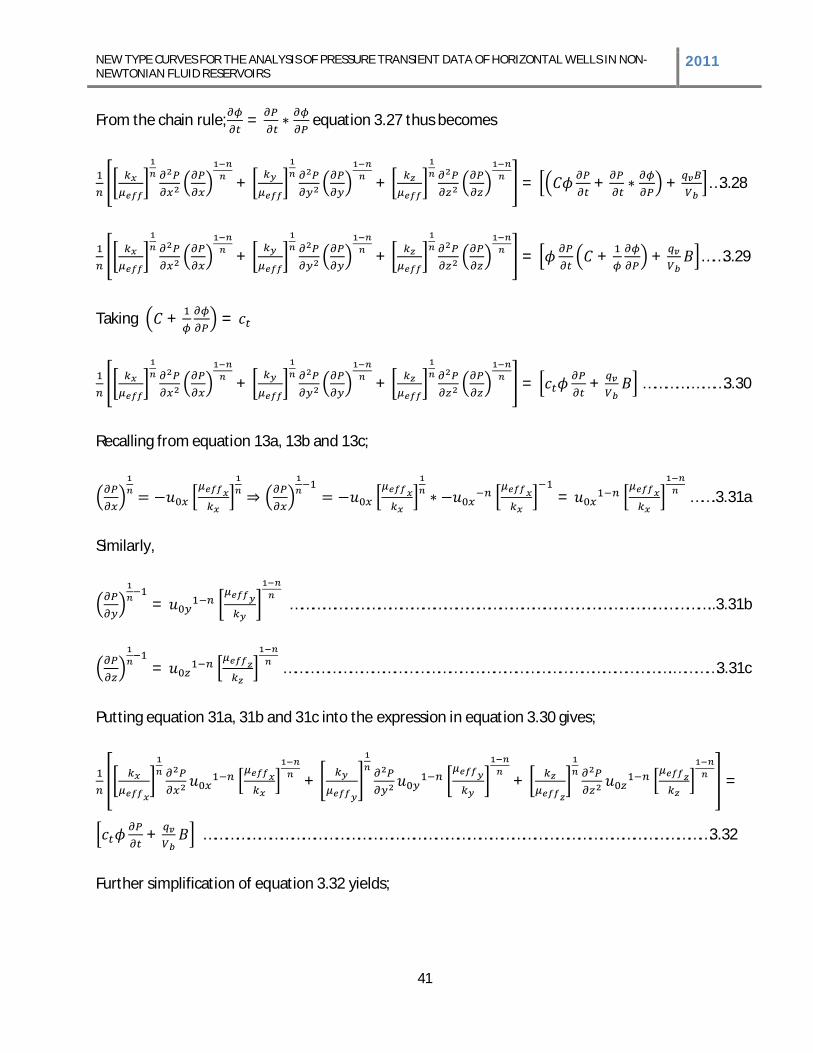
NEW TYPE CURVES FOR THE ANALYSIS OF PRESSURE TRANSIENT DATA OF HORIZONTAL WELLS IN NON-NEWTONIAN FLUID RESERVOIRS 2011
41
From the chain rule; =
equation 3.27 thus becomes
+ + = +
+ …3.28
+ + = + + ……3.29
Taking + =
+ + = + ………….………3.30
Recalling from equation 13a, 13b and 13c;
= …….3.31a
Similarly,
= ……………………………………………………………………………………………………..3.31b
= …………………………………………………………………………………………….…………3.31c
Putting equation 31a, 31b and 31c into the expression in equation 3.30 gives;
+ + =
+ …………………………………………………………………………………………………………………………3.32
Further simplification of equation 3.32 yields;
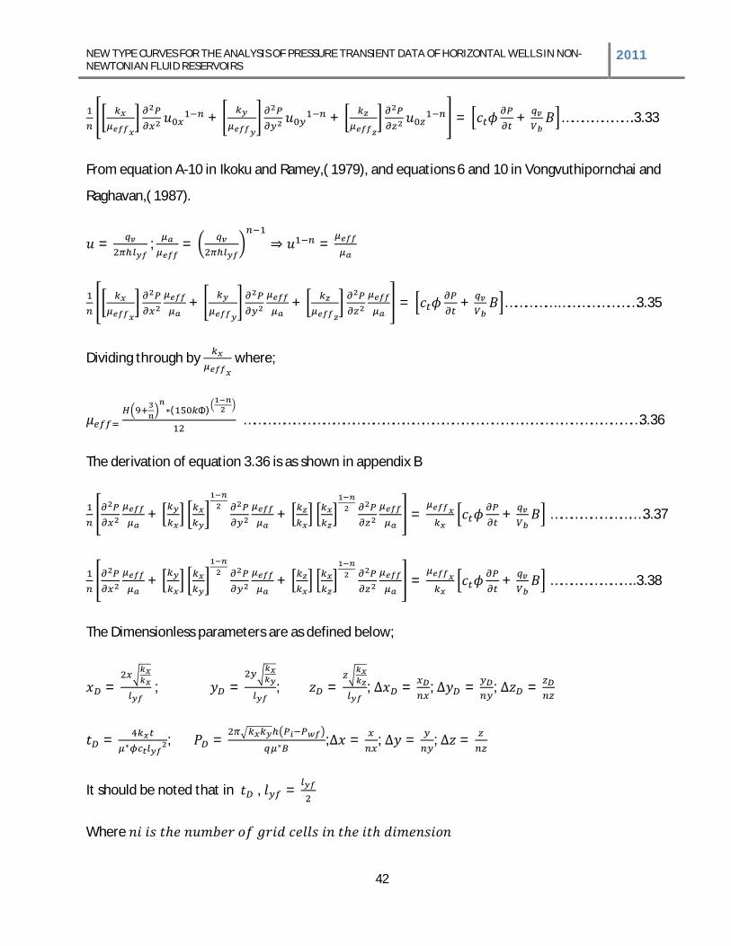
NEW TYPE CURVES FOR THE ANALYSIS OF PRESSURE TRANSIENT DATA OF HORIZONTAL WELLS IN NON-NEWTONIAN FLUID RESERVOIRS 2011
42
+ + = + ………………….3.33
From equation A-10 in Ikoku and Ramey,( 1979), and equations 6 and 10 in Vongvuthipornchai and
Raghavan,( 1987).
= ; = =
+ + = + …………… ……………………3.35
Dividing through by where;
( ) …………………………………………………………………………………………………………3.36
The derivation of equation 3.36 is as shown in appendix B
+ + = + …………………….…3.37
+ + = + ……………………..3.38
The Dimensionless parameters are as defined below;
= ; = ; = ; = ; = ; =
= ; = ; = ; = ; =
It should be noted that in , =
Where
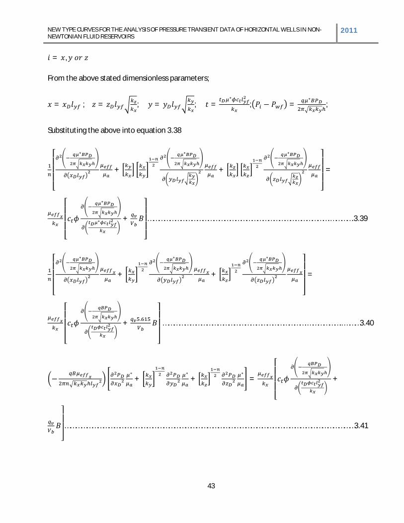
NEW TYPE CURVES FOR THE ANALYSIS OF PRESSURE TRANSIENT DATA OF HORIZONTAL WELLS IN NON-NEWTONIAN FLUID RESERVOIRS 2011
43
= ,
From the above stated dimensionless parameters;
= ; = ; = ; = ; = ;
Substituting the above into equation 3.38
+ + =
+ ……………………………………………………………………………………….………….3.39
+ + =
+ . …………………………………………………………………….………………..………3.40
+ + = +
……………………………………………………………………………………………………………………………………………3.41
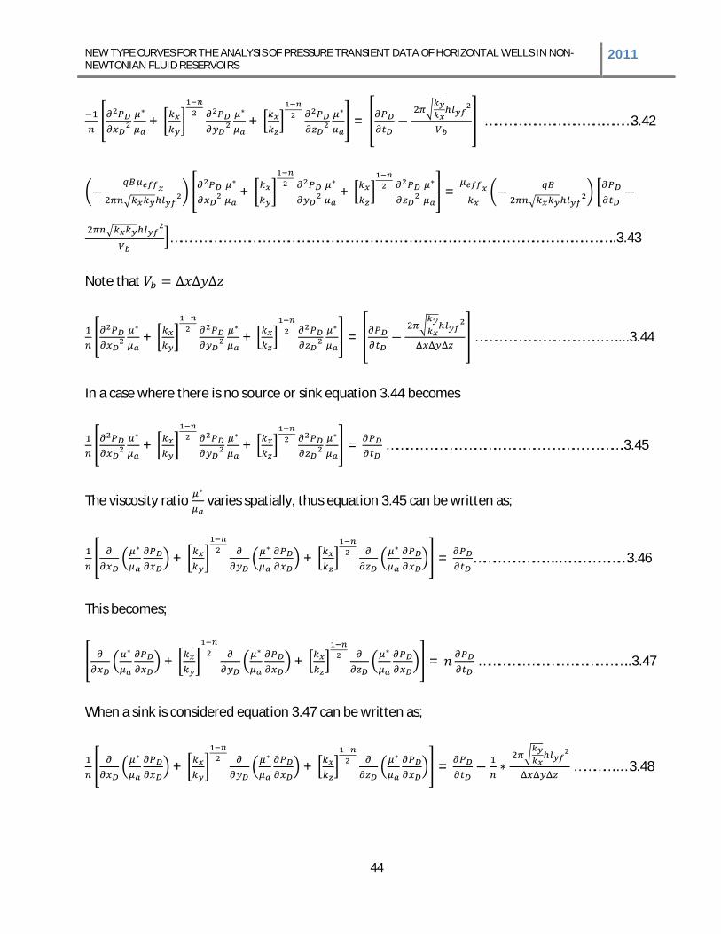
NEW TYPE CURVES FOR THE ANALYSIS OF PRESSURE TRANSIENT DATA OF HORIZONTAL WELLS IN NON-NEWTONIAN FLUID RESERVOIRS 2011
44
+ + =
………………………………………3.42
+ + =
………………………………………………………………………………………………………………………..3.43
Note that
+ + =
……………………………….……....3.44
In a case where there is no source or sink equation 3.44 becomes
+ + = ……………………………………………………………….3.45
The viscosity ratio varies spatially, thus equation 3.45 can be written as;
+ + = ……………………..…………………3.46
This becomes;
+ + = ………………………………………..3.47
When a sink is considered equation 3.47 can be written as;
+ + =
…………..…3.48
NEW TYPE CURVES FOR THE ANALYSIS OF PRESSURE TRANSIENT DATA OF HORIZONTAL WELLS IN NON-NEWTONIAN FLUID RESERVOIRS 2011
45
Equation 3.48 was solved using finite difference approach; however the viscosity ratio is also
dependent on pressure and varies spatially. Equation 3.48 is similar to equation A-15 in
Vongvuthipornchai and Raghavan, (1987).
Equations 5 and 24 in the works of Vongvuthipornchai and Raghavan, (1987) indicate that the
viscosity ratio can be obtained as follow;
+ ……………………………………………………………………………………………………………….…3.49
Thus for a 3 Dimensional system
+ + ………………………………………………………………………………………………………..3.50
Similarly from equation 6 of Vongvuthipornchai and Raghavan, 1987;
= | |…………………………………………………………………………………………………………………………………..3.51
Where H is , the effective viscosity
In equation 24 of the same reference;
= …………………………………………………………………………………………………………..……………3.52
Taking the magnitude of
| | = + + ………………………………………………………………………………………..…….3.53
Substituting equation 3.53 into equation 3.51 gives;
= + + ……………………………………………………………………………3.54
Thus dividing equation 3.52 equation 3.54 yields;
NEW TYPE CURVES FOR THE ANALYSIS OF PRESSURE TRANSIENT DATA OF HORIZONTAL WELLS IN NON-NEWTONIAN FLUID RESERVOIRS 2011
46
=
……………………………………………………………………………………………3.55
= + + ………………………………………………………………3.56
= + + ……………………………………………………………………….3.57
Using the dimensionless terms as defined in equations above;
= + + ……………………..….3.58
= + + ………………………………..3.59
= + + …………………………….……………………….……3.60
= + + …………………………………………………………………..3.61
Equations 3.48 and 3.61 forms the bases of this study following the procedures adopted in the works
of Ikoku and Ramey, 1978 and Vongvuthipornchai and Raghavan, 1987.
3.2.1 BOUNDARY CONDITION
No-flow boundary condition was assumed in the modeling, i.e. the pressure gradient across the
reservoir surface is zero. Equation 3.48 was dicretized using finite difference approach implementing
a no-flow boundary condition across the surface of the reservoir cuboid model. The no-flow
boundary condition as stated below is also discretized to solve equation 3.48 numerically
NEW TYPE CURVES FOR THE ANALYSIS OF PRESSURE TRANSIENT DATA OF HORIZONTAL WELLS IN NON-NEWTONIAN FLUID RESERVOIRS 2011
47
, , ,=
, , ,=
, ,,= 0 ……………..3.62
3.2.2 FINITE DIFFERENCE APPROXIMATION OF MODELLED DIFFERENTIAL EQUATION
Equations 3.48 and 3.61 were solved numerically using the finite difference approach, implementing
the boundary no flow boundary conditions as stated in equation 3.62.
Recalling equation 3.48;
+ + =
……………...3.48
The finite difference discretization of equation 3.48 involves using the central difference
approximation as used in Vongvuthipornchai and Raghavan, 1987 for the spatial derivative and
backward difference approximation for the derivative with respect to time.
, ,
. , . ,
, ,
. , . , +, ,
. , . ,
, ,
. , . , +, ,
. , . ,
, ,
. , . , =
, , , ,
…………………………………………………………………………………………….....3.63
It should be noted that the right hand side (RHS) of equation 3.63 is in the p+1 time iteration. Thus
simplifying equation 3.63 yields the expression below; Equation 3.63 is similar to the finite difference
approximation used in Vongvuthipornchai and Raghavan, 1987 (SPE 13058)
. , , , + , , + , , + , , + , , + , , +
, , . , , , . , + , , . , + , , . , + , , . , +
, , . ,, ,
………………………………………………………………..…………….3.64
NEW TYPE CURVES FOR THE ANALYSIS OF PRESSURE TRANSIENT DATA OF HORIZONTAL WELLS IN NON-NEWTONIAN FLUID RESERVOIRS 2011
48
Re-writing equation 3.64 gives;
. , , , + , , + , , + , , + , , + , , +
, , . , , , . , , , . , , , . , , , . ,
, , . , = , , +
…………………………………………………………………………………….3.65
Where;
=( )
; =( )
; =( )
; = ;
The Boundary condition equation was also discretized using the backward difference approximation
as shown below;
, , , , = , , , , = , , , , = 0 …………………………………………………….……………3.66
the above equation was incorporated into the final development of the linear systems of equation to
aid the solution to the Partial differential equation in equation 3.48.
Depending on the number of grid system being considered, say from 1 to n grid system, a system of
linear equations is obtained from equation 3.65 to obtain an n X n Matrix. In this work, the same
numbers of grids were used in all the dimensions in the x,y and z axis.The linear system of equations
solved was of the form;
[ ] [ ] = [ ] …………………………………………………………………………………………………………………..3.67
Where;
[ ] is the symmetric heptadiagonal coef icient matrix generated from n grids the reservoir model was divided
into
[ ]
[ ]
NEW TYPE CURVES FOR THE ANALYSIS OF PRESSURE TRANSIENT DATA OF HORIZONTAL WELLS IN NON-NEWTONIAN FLUID RESERVOIRS 2011
49
3.2.3 MATLAB R2007b IMPLEMENTATION
A MATLAB R2007b program was written to solve the system of equations generated from equation
3.66 putting into consideration the existing no flow boundary conditions. The MATLAB R2007b code
as shown in Appendix was used to iteratively solve equation 3.67 with respect to time and space in
dimensionless terms. The MATLAB R2007b program was run for a grid size of 15X15X15, which was
the limit of the machine used for the simulation process.
Runs were made basically for a horizontal length of 600ft, 1000ft and 1200ft, a Reservoir size of
3000ft by 3000ft with a height ranging from 100ft to 300ft as would be shown in the next chapter.
Other inputs into the MATLAB code includes the permeabilities , The first set of runs
were made for Newtonian Reservoir fluids, identifying the major flow regimes as discussed in
standard literature, that is the early linear flow, the pseudo-radial flow, the transition flow and the
pseudo steady state flow regimes. Results are as shown in the next chapter.
Consequently, a similar MATLAB R2007b code was written for cases whereby the reservoir fluid is
Non-Newtonian, this new MATLAB R2007b code required written a convergence algorithm for the
viscosity ratio ( ) which varies with pressure. The approach for the convergence algorithm is as
listed below;
Solving systems of equation from equation 3.56 when the reservoir fluid is Newtonian, that is
n=1 and the viscosity ratio = 1 to obtain the dimensionless pressure for the new time step.
The new dimensionless pressure obtained is substituted into discretized version of equation
3.61 as shown in equation 3.68 below to obtain the viscosity ratio for the present time step.
, ,= , , , , + , , , , + , , , ,
………………………………………………………………………………………………………………………………………….3.68
A new system of equations is solved to obtain the viscosity ratio for each of the grid cells
from the substituted dimensionless pressures and permeabilities.
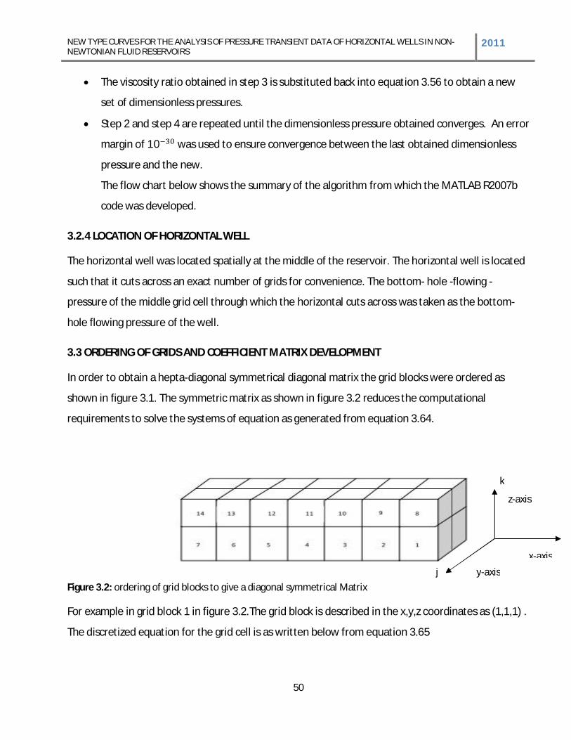
NEW TYPE CURVES FOR THE ANALYSIS OF PRESSURE TRANSIENT DATA OF HORIZONTAL WELLS IN NON-NEWTONIAN FLUID RESERVOIRS 2011
50
The viscosity ratio obtained in step 3 is substituted back into equation 3.56 to obtain a new
set of dimensionless pressures.
Step 2 and step 4 are repeated until the dimensionless pressure obtained converges. An error
margin of 10 was used to ensure convergence between the last obtained dimensionless
pressure and the new.
The flow chart below shows the summary of the algorithm from which the MATLAB R2007b
code was developed.
3.2.4 LOCATION OF HORIZONTAL WELL
The horizontal well was located spatially at the middle of the reservoir. The horizontal well is located
such that it cuts across an exact number of grids for convenience. The bottom- hole -flowing -
pressure of the middle grid cell through which the horizontal cuts across was taken as the bottom-
hole flowing pressure of the well.
3.3 ORDERING OF GRIDS AND COEFFICIENT MATRIX DEVELOPMENT
In order to obtain a hepta-diagonal symmetrical diagonal matrix the grid blocks were ordered as
shown in figure 3.1. The symmetric matrix as shown in figure 3.2 reduces the computational
requirements to solve the systems of equation as generated from equation 3.64.
Figure 3.2: ordering of grid blocks to give a diagonal symmetrical Matrix
For example in grid block 1 in figure 3.2.The grid block is described in the x,y,z coordinates as (1,1,1) .
The discretized equation for the grid cell is as written below from equation 3.65
j x-axis
z-axis
y-axis
k
NEW TYPE CURVES FOR THE ANALYSIS OF PRESSURE TRANSIENT DATA OF HORIZONTAL WELLS IN NON-NEWTONIAN FLUID RESERVOIRS 2011
51
. , , , + , , + , , + , , + , , + , , + , , . ,
, , . , , , . , , , . , , , . , , , . , = , , +
…………………………………………………………………………………………………………………….………….…3.69
The boundary conditions apply on this grid cell, thus for this grid cell the boundary can be written as
below from equation 3.66;
= 1, = 1 = 1
, , , , = , , , , = , , , , = 0 …………………………………………………..……………….……3.70
Thus equation 3.70 becomes;
, , = , , = , , = , , ………………………………………………………………………………………………3.71
Substituting the boundary conditions in equation 3.71 into equation 3.69 yield;
. , , , + , , + , , + , , . , , , . , , , . , =
, , +
… ………………………………………………………………………………………………………………….3.72
In a similar manner, the discretization for the second grid cell 2 when = 2, = 1, = 1 can be
written as follows;
. , , , + , , + , , + , , + , , + , , + , , . ,
, , . , , , . , , , . , , , . , , , . , = , , +
……………………………………………………………………………………………………………………….………….3.73
Implementing the boundary conditions in a similar way as shown in equation 3.70 gives
= 2, = 1 = 1
NEW TYPE CURVES FOR THE ANALYSIS OF PRESSURE TRANSIENT DATA OF HORIZONTAL WELLS IN NON-NEWTONIAN FLUID RESERVOIRS 2011
52
, , , , = , , , , = 0 ……………………………………………………………..………………………………3.74
Thus;
, , = , , = , , ………………………………………………………………………………………………………….3.75
Substituting equation into equation 3.73 gives;
. , , , + , , + , , + , , + , , . , , , . ,
, , . , , , . , = , , +
………………………………………………………………..3.76
The seventh grid is located at a position where = 7, = 1, = 1 as shown in figure 3.1 can also be
discretized similarly as shown below;
= 7, = 1 = 1
. , , , + , , + , , + , , + , , + , , + , , . ,
, , . , , , . , , , . , , , . , , , . , = , , +
…………………….……………………………………………………………………………………………………………………………..…3.77
Boundary conditions can is implemented for the last grid cell as shown below;
, , = , , = , , ……………………………………………………………………………………………………………3.78
At the last grid cell a special boundary condition is used to ensure consistency
, , = , , …………………………………………………………………………………………………………………………...3.79
The process is repeated for all the grid cells in the modeled and the system of equations of equation
developed is express as matrix and solved. The hepta-diagonal coefficient matrix developed for the 3-
dimensional model has the pattern.
NEW TYPE CURVES FOR THE ANALYSIS OF PRESSURE TRANSIENT DATA OF HORIZONTAL WELLS IN NON-NEWTONIAN FLUID RESERVOIRS 2011
53
3.4 TYPE CURVE DEVELOPMENT
Type curves were obtained by running the MATLAB 7.5.0 (R2007b) codes developed for horizontal
well lengths of 600ft, 1000ft and 1200ft for n=0.1 to n=1. The effect of permeability heterogeneity
was also considered by running the MATLAB program for = 100 , = 50 = 25 and
when = 75 , = 75 = 75 for the various values of n being considered. The type-curves
obtained are as shown in the next chapter. It should be noted that the position of the Horizontal well
was not changed in obtaining any of these type-curves
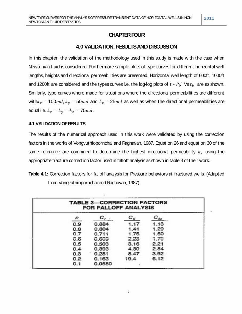
NEW TYPE CURVES FOR THE ANALYSIS OF PRESSURE TRANSIENT DATA OF HORIZONTAL WELLS IN NON-NEWTONIAN FLUID RESERVOIRS
2011
54
CHAPTER FOUR
4.0 VALIDATION, RESULTS AND DISCUSSION
In this chapter, the validation of the methodology used in this study is made with the case when
Newtonian fluid is considered. Furthermore sample plots of type curves for different horizontal well
lengths, heights and directional permeabilities are presented. Horizontal well length of 600ft, 1000ft
and 1200ft are considered and the types curves i.e. the log-log plots of Vs are as shown.
Similarly, type curves where made for situations where the directional permeabilities are different
with = 100 , = 50 and = 25 as well as when the directional permeabilities are
equal i.e. = = = 75 .
4.1 VALIDATION OF RESULTS
The results of the numerical approach used in this work were validated by using the correction
factors in the works of Vongvuthiopornchai and Raghavan, 1987. Equation 26 and equation 30 of the
same reference are combined to determine the highest directional permeability using the
appropriate fracture correction factor used in falloff analysis as shown in table 3 of their work.
Table 4.1: Correction factors for falloff analysis for Pressure behaviors at fractured wells. (Adapted
from Vongvuthiopornchai and Raghavan, 1987)
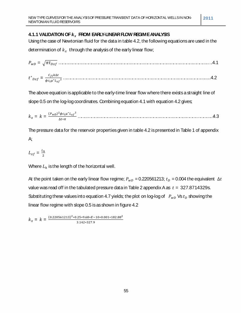
NEW TYPE CURVES FOR THE ANALYSIS OF PRESSURE TRANSIENT DATA OF HORIZONTAL WELLS IN NON-NEWTONIAN FLUID RESERVOIRS 2011
55
4.1.1 VALIDATION OF FROM EARLY-LINEAR FLOW REGIME ANALYSIS Using the case of Newtonian fluid for the data in table 4.2, the following equations are used in the
determination of through the analysis of the early linear flow;
= ………………………………………………………………………………………………………………………..….4.1
= …………………………………………………………………………………………………………………......4.2
The above equation is applicable to the early-time linear flow where there exists a straight line of
slope 0.5 on the log-log coordinates. Combining equation 4.1 with equation 4.2 gives;
= =( )
……………………………………………………………………………………………….……………4.3
The pressure data for the reservoir properties given in table 4.2 is presented in Table 1 of appendix
A;
=
Where is the length of the horizontal well.
At the point taken on the early linear flow regime; =0.220561213; =0.004 the equivalent
value was read off in the tabulated pressure data in Table 2 appendix A as = 327.8714329s.
Substituting these values into equation 4.7 yields; the plot on log-log of Vs showing the
linear flow regime with slope 0.5 is as shown in figure 4.2
= = ( . ) . . . .. .
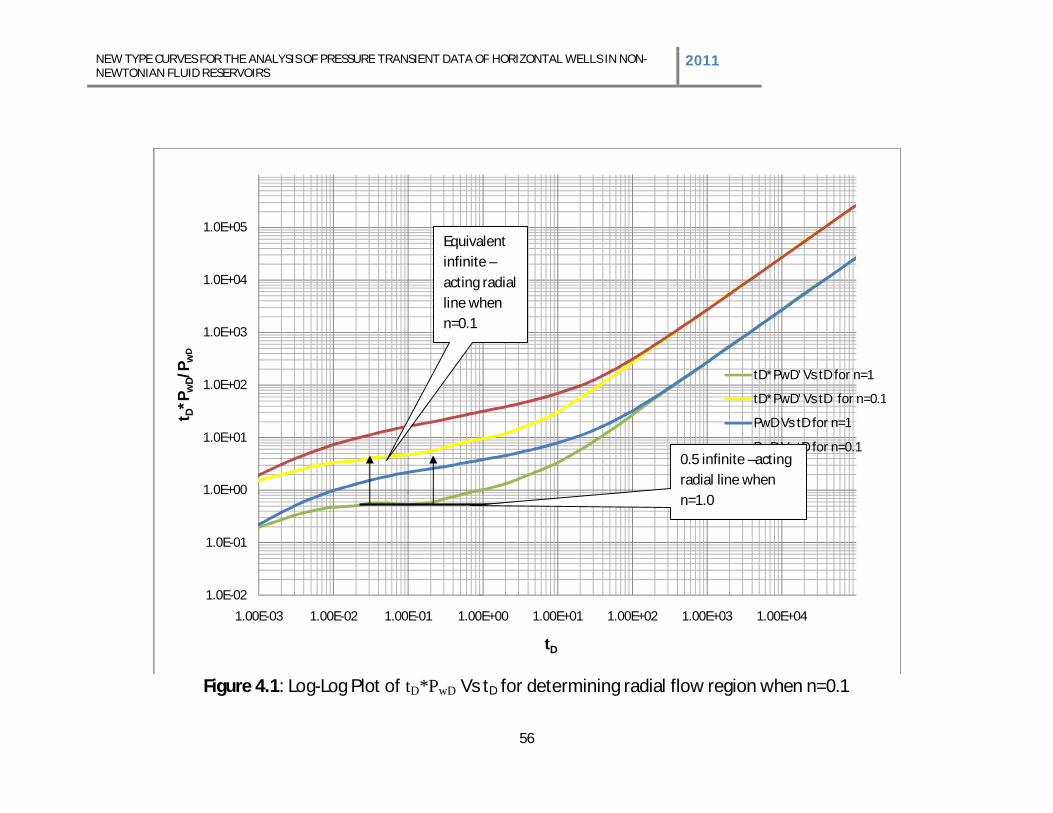
NEW TYPE CURVES FOR THE ANALYSIS OF PRESSURE TRANSIENT DATA OF HORIZONTAL WELLS IN NON-NEWTONIAN FLUID RESERVOIRS
2011
56
Figure 4.1: Log-Log Plot of tD*PwD Vs tD for determining radial flow region when n=0.1
1.0E-02
1.0E-01
1.0E+00
1.0E+01
1.0E+02
1.0E+03
1.0E+04
1.0E+05
1.00E-03 1.00E-02 1.00E-01 1.00E+00 1.00E+01 1.00E+02 1.00E+03 1.00E+04
t D*P
wD/
P wD
tD
tD*PwD' Vs tD for n=1
tD*PwD' Vs tD for n=0.1
PwD Vs tD for n=1
PwD Vs tD for n=0.10.5 infinite –acting radial line when n=1.0
Equivalent infinite –acting radial line when n=0.1
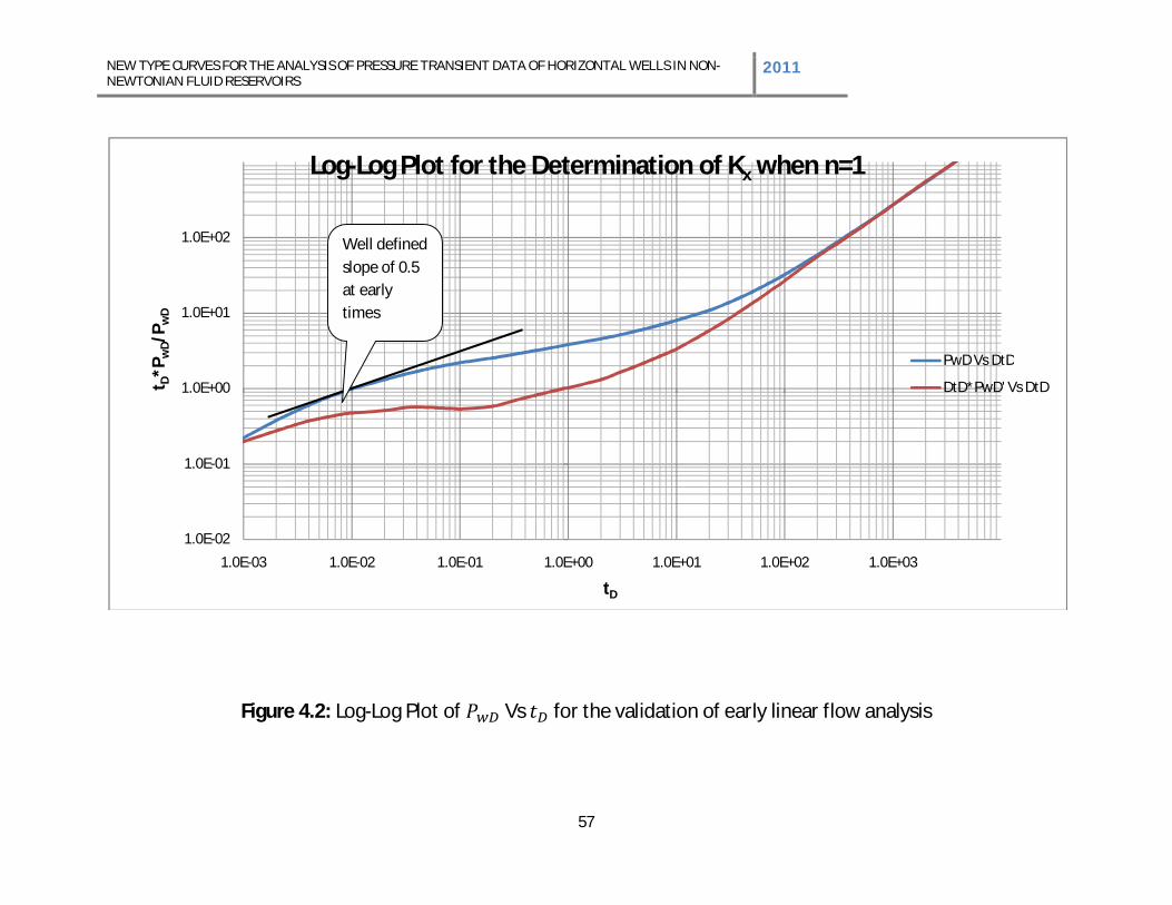
NEW TYPE CURVES FOR THE ANALYSIS OF PRESSURE TRANSIENT DATA OF HORIZONTAL WELLS IN NON-NEWTONIAN FLUID RESERVOIRS 2011
57
Figure 4.2: Log-Log Plot of Vs for the validation of early linear flow analysis
1.0E-02
1.0E-01
1.0E+00
1.0E+01
1.0E+02
1.0E-03 1.0E-02 1.0E-01 1.0E+00 1.0E+01 1.0E+02 1.0E+03
t D*P
wD/
P wD
tD
Log-Log Plot for the Determination of Kx when n=1
PwD Vs DtD
DtD*PwD' Vs DtD
Well defined slope of 0.5 at early times
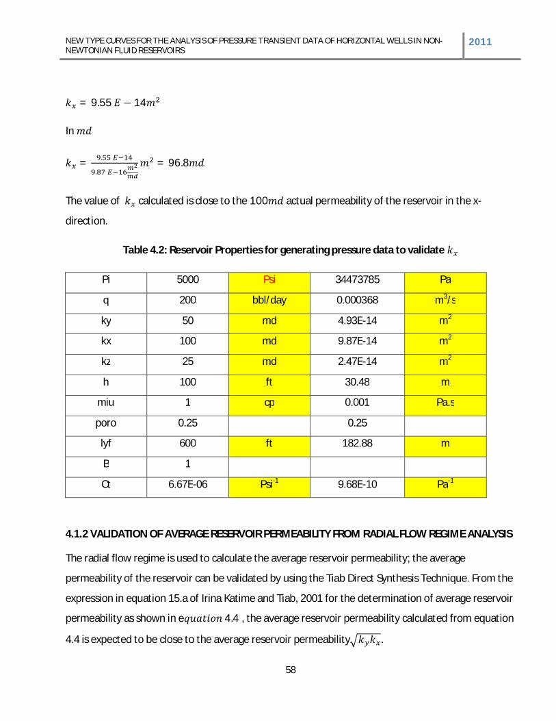
NEW TYPE CURVES FOR THE ANALYSIS OF PRESSURE TRANSIENT DATA OF HORIZONTAL WELLS IN NON-NEWTONIAN FLUID RESERVOIRS
2011
58
= 9.55 14
In
= .
. = 96.8
The value of calculated is close to the 100 actual permeability of the reservoir in the x-
direction.
Table 4.2: Reservoir Properties for generating pressure data to validate
Pi 5000 Psi 34473785 Pa
q 200 bbl/day 0.000368 m3/s
ky 50 md 4.93E-14 m2
kx 100 md 9.87E-14 m2
kz 25 md 2.47E-14 m2
h 100 ft 30.48 m
miu 1 cp 0.001 Pa.s
poro 0.25
0.25
lyf 600 ft 182.88 m
B 1
Ct 6.67E-06 Psi-1 9.68E-10 Pa-1
4.1.2 VALIDATION OF AVERAGE RESERVOIR PERMEABILITY FROM RADIAL FLOW REGIME ANALYSIS
The radial flow regime is used to calculate the average reservoir permeability; the average
permeability of the reservoir can be validated by using the Tiab Direct Synthesis Technique. From the
expression in equation 15.a of Irina Katime and Tiab, 2001 for the determination of average reservoir
permeability as shown in e 4.4 , the average reservoir permeability calculated from equation
4.4 is expected to be close to the average reservoir permeability .
NEW TYPE CURVES FOR THE ANALYSIS OF PRESSURE TRANSIENT DATA OF HORIZONTAL WELLS IN NON-NEWTONIAN FLUID RESERVOIRS 2011
59
= 0.5( ) ( )
………………………………………………………………………………………………..…………….4.4
Where ( ) is the value of for the infinite acting radial flow at t
The reservoir properties are as shown in table 4.2 above
The value of t* P' at the infinite acting radial flow is read from the plot in figure 4.3 or read from
the table 2 in Appendix A as 13634.02 substituting this and other reservoir parameters into equation
4 yields;
= 0.5 .. ( . )
Using = 0.001Pa. s
Thus;
= 7.0469 14
Converting k to md gives;
= .
.= 71.4md
The actual average reservoir permeability can be computed from the values given in table
4.2 above.
= = 100 50 = 70.71068md
The Value of the average permeability calculated using the Tiab’s direct synthesis Technique is close
to the actual reservoir permeability.
4.1.3 VALIDATION OF DRAINAGE AREA FROM PSEUDO STEADY STATE FLOW REGIME ANALYSIS.
The Drainage area can be obtained from the Pseudo steady state flow regime. The expression for
calculating drainage area for a horizontal well is as presented below;
NEW TYPE CURVES FOR THE ANALYSIS OF PRESSURE TRANSIENT DATA OF HORIZONTAL WELLS IN NON-NEWTONIAN FLUID RESERVOIRS 2011
60
= ……………………………………………………………………………………………………………4.5
A value of is read off from the Pseudo steady state flow regime from figure 4.4 and the
corresponding t value is read off from figure 4 or obtained from table 2 in the appendix A. A value of
= 21384.34 at =6557428658 is read off. Thus;
= . . .. . . .
= 760,765.9
The value of the drainage area calculated is fairly close to the actual area of the reservoir.
The actual area of the reservoir is;
(3000 0.3048) (3000 0.3048) = 836,127.36
4.2 APPLICATIONS TO NON-NEWTONIAN RESERVOIR FLUIDS The pressure data as obtained from the simulation study in this work can be applied to established
methods in the works of Igbokoyi and Tiab, 2007; Irina Katime and Tiab, 2001 and Vongvuthipornchai
and Raghavan, 1987.
4.2.1 ANALYSIS OF EARLY LINEAR FLOW REGIME FOR THE DETERMINATION OF
From equation 26 of Vongvuthiopornchai and Raghavan, 1987;
= ………………………………………………………………………………………………………………….…4.6
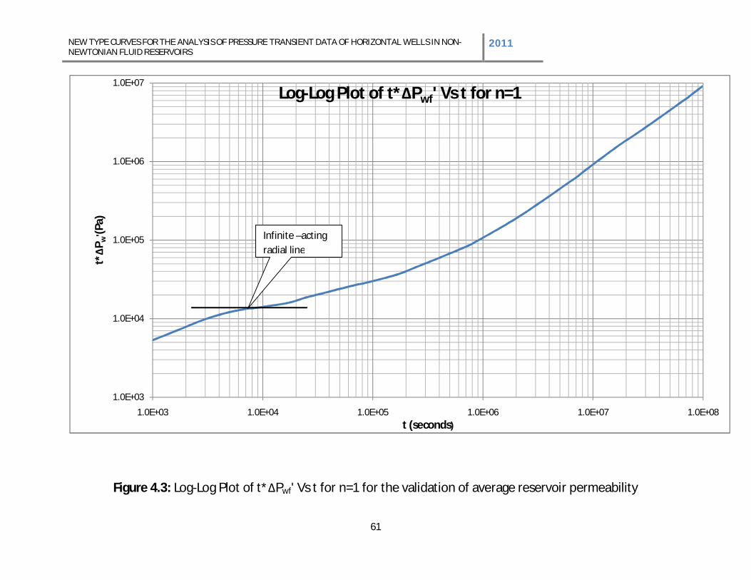
NEW TYPE CURVES FOR THE ANALYSIS OF PRESSURE TRANSIENT DATA OF HORIZONTAL WELLS IN NON-NEWTONIAN FLUID RESERVOIRS
2011
61
Figure 4.3: Log-Log Plot of t* Pwf' Vs t for n=1 for the validation of average reservoir permeability
1.0E+03
1.0E+04
1.0E+05
1.0E+06
1.0E+07
1.0E+03 1.0E+04 1.0E+05 1.0E+06 1.0E+07 1.0E+08
t*P w
'(Pa)
t (seconds)
Log-Log Plot of t* Pwf' Vs t for n=1
Infinite –acting radial line
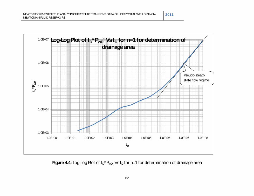
NEW TYPE CURVES FOR THE ANALYSIS OF PRESSURE TRANSIENT DATA OF HORIZONTAL WELLS IN NON-NEWTONIAN FLUID RESERVOIRS
2011
62
Figure 4.4: Log-Log Plot of tD*PwD' Vs tD for n=1 for determination of drainage area
1.0E+03
1.0E+04
1.0E+05
1.0E+06
1.0E+07
1.0E+00 1.0E+01 1.0E+02 1.0E+03 1.0E+04 1.0E+05 1.0E+06 1.0E+07 1.0E+08
t D*P
wD'
tD
Log-Log Plot of tD*PwD' Vs tD for n=1 for determination of drainage area
Pseudo-steady state flow regime
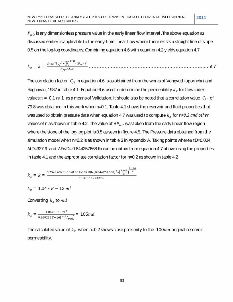
NEW TYPE CURVES FOR THE ANALYSIS OF PRESSURE TRANSIENT DATA OF HORIZONTAL WELLS IN NON-NEWTONIAN FLUID RESERVOIRS
2011
63
is any dimensionless pressure value in the early linear flow interval .The above equation as
discussed earlier is applicable to the early-time linear flow where there exists a straight line of slope
0.5 on the log-log coordinates. Combining equation 4.6 with equation 4.2 yields equation 4.7
= =( )
……………………………………………………………………………………………….……4.7
The correlation factor in equation 4.6 is as obtained from the works of Vongvuthiopornchai and
Raghavan, 1987 in table 4.1. Equation 6 is used to determine the permeability for flow index
values = 0.1 1 as a means of Validation. It should also be noted that a correlation value of
79.8 was obtained in this work when n=0.1. Table 4.1 shows the reservoir and fluid properties that
was used to obtain pressure data when equation 4.7 was used to compute for n=0.2 and other
values of n as shown in table 4.2. The value of was taken from the early linear flow region
where the slope of the log-log plot is 0.5 as seen in figure 4.5. The Pressure data obtained from the
simulation model when n=0.2 is as shown in table 3 in Appendix A. Taking points where tD=0.004,
tD=327.9 and PwD= 0.844257668 Kx can be obtain from equation 4.7 above using the properties
in table 4.1 and the appropriate correlation factor for n=0.2 as shown in table 4.2
= =. . . . ( . ) .
.
. . .
= 1.04 13
Converting to
= .
.= 105
The calculated value of when n=0.2 shows close proximity to the 100 original reservoir
permeability.
NEW TYPE CURVES FOR THE ANALYSIS OF PRESSURE TRANSIENT DATA OF HORIZONTAL WELLS IN NON-NEWTONIAN FLUID RESERVOIRS
2011
64
Figure 4.5: Log-Log plot of PwD Vs tD for the determination of Kx when n=0.2
1.0E-01
1.0E+00
1.0E+01
1.0E+02
1.0E+03
1.0E+04
1.0E+05
1.0E+06
1.00E-03 1.00E-02 1.00E-01 1.00E+00 1.00E+01 1.00E+02 1.00E+03 1.00E+04
P wD
tD
Log-Log Plot of PwD Vs tD for n=0.2
Early linear flow regime
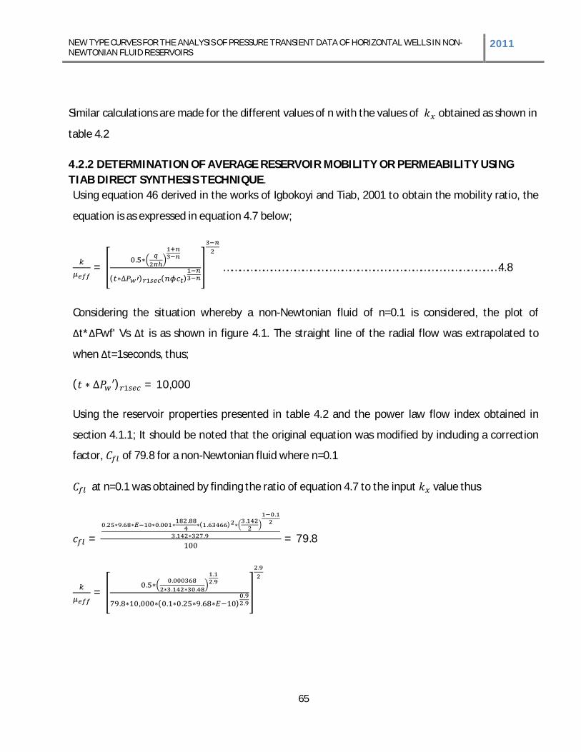
NEW TYPE CURVES FOR THE ANALYSIS OF PRESSURE TRANSIENT DATA OF HORIZONTAL WELLS IN NON-NEWTONIAN FLUID RESERVOIRS
2011
65
Similar calculations are made for the different values of n with the values of obtained as shown in
table 4.2
4.2.2 DETERMINATION OF AVERAGE RESERVOIR MOBILITY OR PERMEABILITY USING TIAB DIRECT SYNTHESIS TECHNIQUE. Using equation 46 derived in the works of Igbokoyi and Tiab, 2001 to obtain the mobility ratio, the
equation is as expressed in equation 4.7 below;
=.
( ) ( ) ……………………………………………………………………………………………4.8
Considering the situation whereby a non-Newtonian fluid of n=0.1 is considered, the plot of
t* Pwf' Vs t is as shown in figure 4.1. The straight line of the radial flow was extrapolated to
when t=1seconds, thus;
( ) = 10,000
Using the reservoir properties presented in table 4.2 and the power law flow index obtained in
section 4.1.1; It should be noted that the original equation was modified by including a correction
factor, of 79.8 for a non-Newtonian fluid where n=0.1
at n=0.1 was obtained by finding the ratio of equation 4.7 to the input value thus
=. . . . ( . ) .
.
. . = 79.8
=. .
. .
.
.
. , ( . . . )..
.
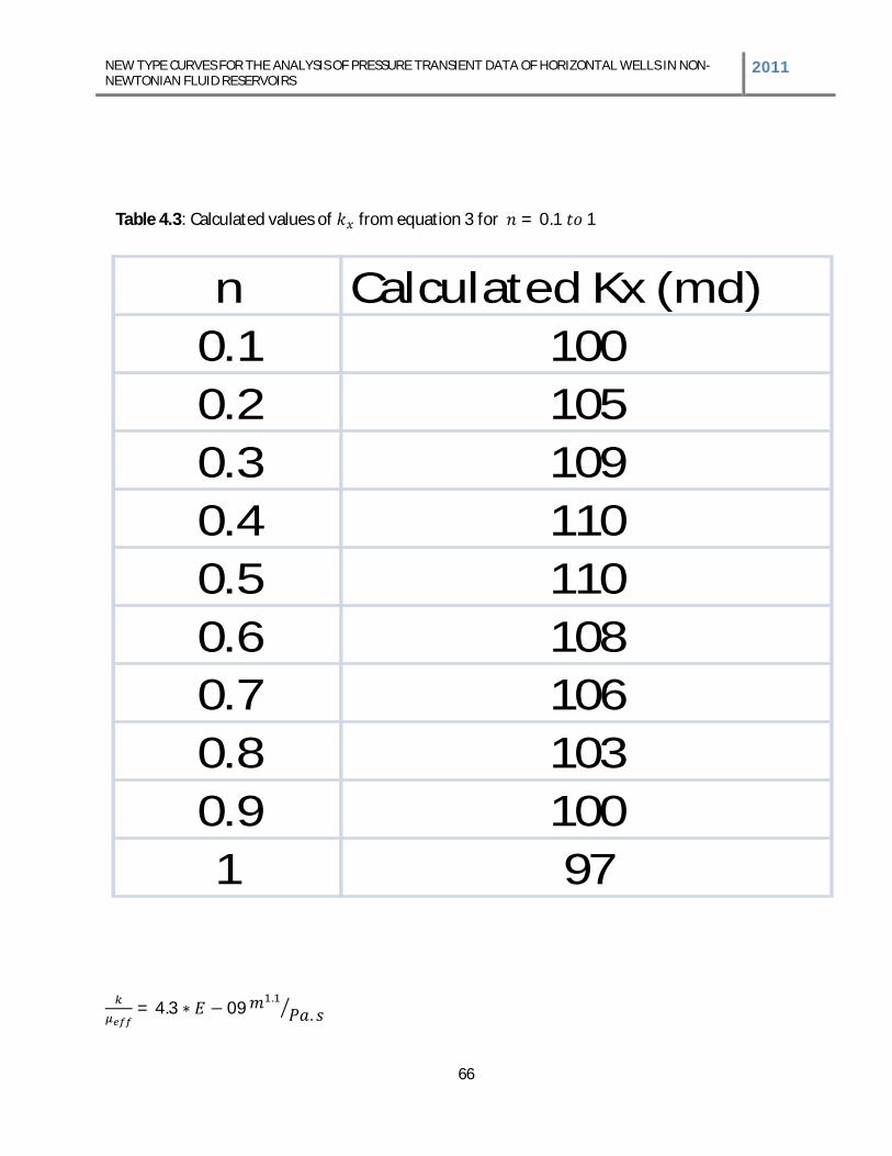
NEW TYPE CURVES FOR THE ANALYSIS OF PRESSURE TRANSIENT DATA OF HORIZONTAL WELLS IN NON-NEWTONIAN FLUID RESERVOIRS 2011
66
Table 4.3: Calculated values of from equation 3 for = 0.1 1
n Calculated Kx (md)0.1 1000.2 1050.3 1090.4 1100.5 1100.6 1080.7 1060.8 1030.9 1001 97
= 4.3 09.
.
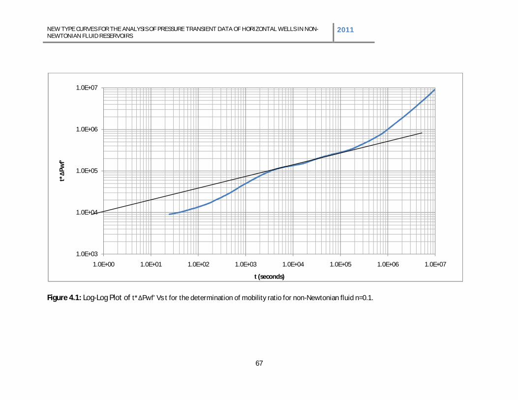
NEW TYPE CURVES FOR THE ANALYSIS OF PRESSURE TRANSIENT DATA OF HORIZONTAL WELLS IN NON-NEWTONIAN FLUID RESERVOIRS
2011
67
Figure 4.1: Log-Log Plot of t* Pwf' Vs t for the determination of mobility ratio for non-Newtonian fluid n=0.1.
1.0E+03
1.0E+04
1.0E+05
1.0E+06
1.0E+07
1.0E+00 1.0E+01 1.0E+02 1.0E+03 1.0E+04 1.0E+05 1.0E+06 1.0E+07
t*Pw
f'
t (seconds)
NEW TYPE CURVES FOR THE ANALYSIS OF PRESSURE TRANSIENT DATA OF HORIZONTAL WELLS IN NON-NEWTONIAN FLUID RESERVOIRS
2011
68
Thus the average reservoir mobility is;
= . 4.3 09.
.
4.3 DEVELOPMENT OF TYPE CURVES
Type curves including log-log plots of were made for different
horizontal well lengths, reservoir thickness, directional permeabilities and flow index n. regimes. As
the flow index increase from = 0.1 1.0 as would be shown in the next sections.
4.3.1 Horizontal Well length of 600ft = , = = =
Type curves were made for cases where the flow index vary from = 0.1 1.0 as shown in the log-
log plots of dimensionless pressure plots against dimensionless time in figure 4.6 as well as the plots
of log-log dimensionless pressure derivative plots as shown in figure 4.7. From the plots it can be
seen that as the flow index n decreases from 1.0 to 0.1 the pressure drop increases. Although the
flow regimes are obvious for the Newtonian plots, they are not obvious for the non-Newtonian case.
The type curves when n=0.9 to 0.7 are similar to when n=1.0 the pseudo Steady state flow regime
exist for all values of n.
4.3.2 Horizontal Well length of 1000ft = , = = =
The type-curve for the case whereby the horizontal well length is 1000ft is as presented in figure 4.8-
4.9 For flow index n=0.1 to 1.0. In the derivative log-log plots the early radial flow is absent, but the,
Pseudo radial flow, early linear, a transition zone and pseudo steady state flow regimes can be seen
in the plots. Similarly as for the case when the horizontal well was 600ft, the pressure drop increased
as the non-Newtonian flow index n decreased. Also as the value of n tends to 1 the type curve and
log-log pressure drop plots are similar. The value of increases from the 0.5 the
Newtonian value as the value of n increases from 0.1 to 0.9
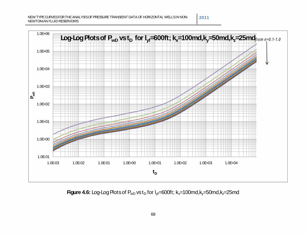
NEW TYPE CURVES FOR THE ANALYSIS OF PRESSURE TRANSIENT DATA OF HORIZONTAL WELLS IN NON-NEWTONIAN FLUID RESERVOIRS
2011
69
Figure 4.6: Log-Log Plots of PwD vs tD for lyf=600ft; kx=100md,ky=50md,kz=25md
1.0E-01
1.0E+00
1.0E+01
1.0E+02
1.0E+03
1.0E+04
1.0E+05
1.0E+06
1.0E-03 1.0E-02 1.0E-01 1.0E+00 1.0E+01 1.0E+02 1.0E+03 1.0E+04
P wD
tD
Log-Log Plots of PwD vs tD for lyf=600ft; kx=100md,ky=50md,kz=25mdfrom n=0.1-1.0
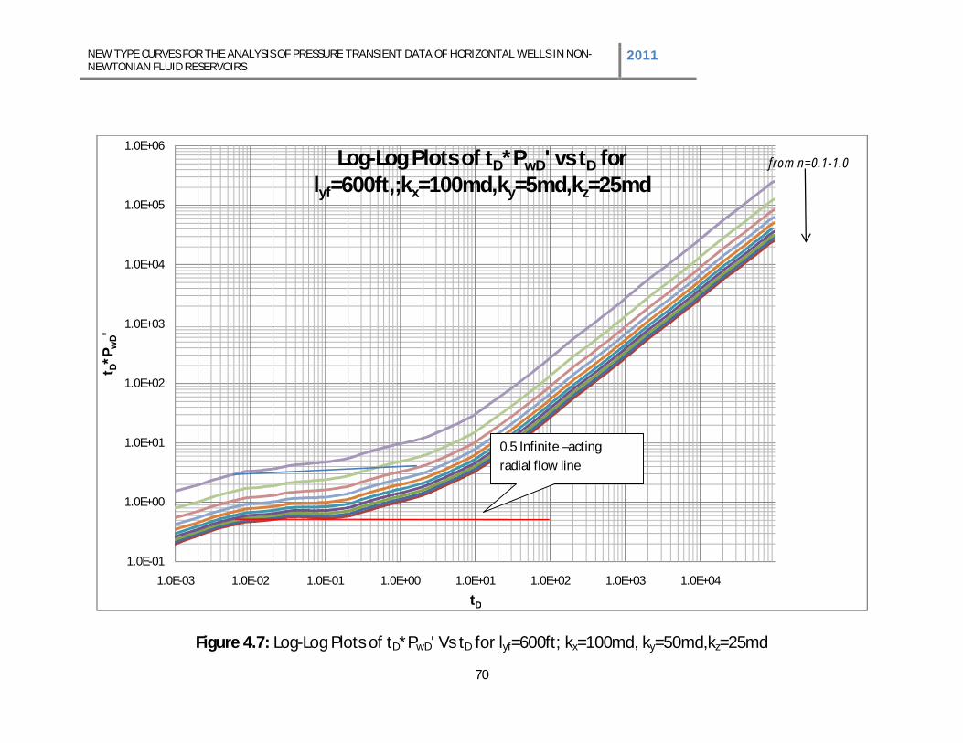
NEW TYPE CURVES FOR THE ANALYSIS OF PRESSURE TRANSIENT DATA OF HORIZONTAL WELLS IN NON-NEWTONIAN FLUID RESERVOIRS
2011
70
Figure 4.7: Log-Log Plots of tD*PwD' Vs tD for lyf=600ft; kx=100md, ky=50md,kz=25md
1.0E-01
1.0E+00
1.0E+01
1.0E+02
1.0E+03
1.0E+04
1.0E+05
1.0E+06
1.0E-03 1.0E-02 1.0E-01 1.0E+00 1.0E+01 1.0E+02 1.0E+03 1.0E+04
t D*P
wD'
tD
Log-Log Plots of tD*PwD' vs tD for lyf=600ft,;kx=100md,ky=5md,kz=25md
from n=0.1-1.0
0.5 Infinite –acting radial flow line
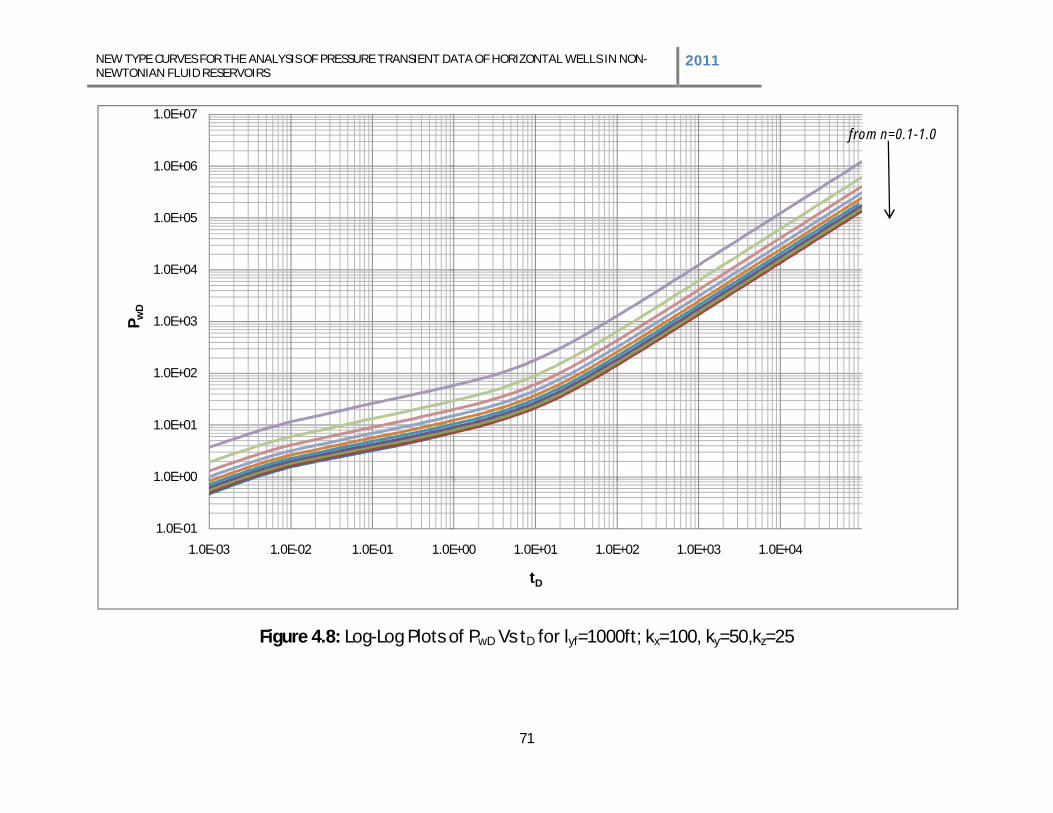
NEW TYPE CURVES FOR THE ANALYSIS OF PRESSURE TRANSIENT DATA OF HORIZONTAL WELLS IN NON-NEWTONIAN FLUID RESERVOIRS 2011
71
Figure 4.8: Log-Log Plots of PwD Vs tD for lyf=1000ft; kx=100, ky=50,kz=25
1.0E-01
1.0E+00
1.0E+01
1.0E+02
1.0E+03
1.0E+04
1.0E+05
1.0E+06
1.0E+07
1.0E-03 1.0E-02 1.0E-01 1.0E+00 1.0E+01 1.0E+02 1.0E+03 1.0E+04
P wD
tD
from n=0.1-1.0
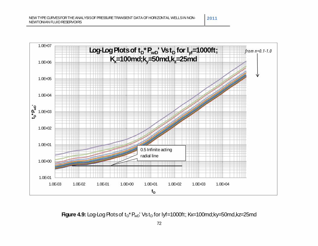
NEW TYPE CURVES FOR THE ANALYSIS OF PRESSURE TRANSIENT DATA OF HORIZONTAL WELLS IN NON-NEWTONIAN FLUID RESERVOIRS 2011
72
Figure 4.9: Log-Log Plots of tD*PwD' Vs tD for lyf=1000ft; Kx=100md;ky=50md,kz=25md
1.0E-01
1.0E+00
1.0E+01
1.0E+02
1.0E+03
1.0E+04
1.0E+05
1.0E+06
1.0E+07
1.0E-03 1.0E-02 1.0E-01 1.0E+00 1.0E+01 1.0E+02 1.0E+03 1.0E+04
t D*P
wD'
tD
Log-Log Plots of tD*PwD' Vs tD for lyf=1000ft; Kx=100md;ky=50md,kz=25md
from n=0.1-1.0
0.5 Infinite acting radial line
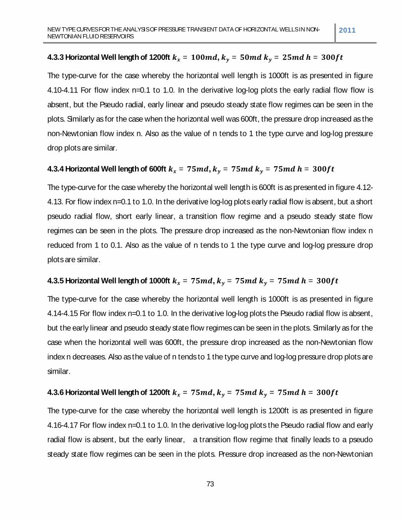
NEW TYPE CURVES FOR THE ANALYSIS OF PRESSURE TRANSIENT DATA OF HORIZONTAL WELLS IN NON-NEWTONIAN FLUID RESERVOIRS
2011
73
4.3.3 Horizontal Well length of 1200ft = , = = =
The type-curve for the case whereby the horizontal well length is 1000ft is as presented in figure
4.10-4.11 For flow index n=0.1 to 1.0. In the derivative log-log plots the early radial flow flow is
absent, but the Pseudo radial, early linear and pseudo steady state flow regimes can be seen in the
plots. Similarly as for the case when the horizontal well was 600ft, the pressure drop increased as the
non-Newtonian flow index n. Also as the value of n tends to 1 the type curve and log-log pressure
drop plots are similar.
4.3.4 Horizontal Well length of 600ft = , = = =
The type-curve for the case whereby the horizontal well length is 600ft is as presented in figure 4.12-
4.13. For flow index n=0.1 to 1.0. In the derivative log-log plots early radial flow is absent, but a short
pseudo radial flow, short early linear, a transition flow regime and a pseudo steady state flow
regimes can be seen in the plots. The pressure drop increased as the non-Newtonian flow index n
reduced from 1 to 0.1. Also as the value of n tends to 1 the type curve and log-log pressure drop
plots are similar.
4.3.5 Horizontal Well length of 1000ft = , = = =
The type-curve for the case whereby the horizontal well length is 1000ft is as presented in figure
4.14-4.15 For flow index n=0.1 to 1.0. In the derivative log-log plots the Pseudo radial flow is absent,
but the early linear and pseudo steady state flow regimes can be seen in the plots. Similarly as for the
case when the horizontal well was 600ft, the pressure drop increased as the non-Newtonian flow
index n decreases. Also as the value of n tends to 1 the type curve and log-log pressure drop plots are
similar.
4.3.6 Horizontal Well length of 1200ft = , = = =
The type-curve for the case whereby the horizontal well length is 1200ft is as presented in figure
4.16-4.17 For flow index n=0.1 to 1.0. In the derivative log-log plots the Pseudo radial flow and early
radial flow is absent, but the early linear, a transition flow regime that finally leads to a pseudo
steady state flow regimes can be seen in the plots. Pressure drop increased as the non-Newtonian

NEW TYPE CURVES FOR THE ANALYSIS OF PRESSURE TRANSIENT DATA OF HORIZONTAL WELLS IN NON-NEWTONIAN FLUID RESERVOIRS 2011
74
flow index n decreases. Also as the value of n tends to 1 the type curve and log-log pressure drop
plots are similar.
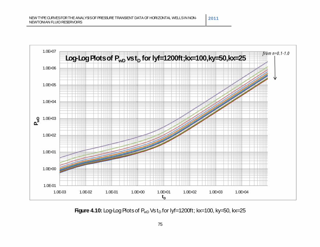
NEW TYPE CURVES FOR THE ANALYSIS OF PRESSURE TRANSIENT DATA OF HORIZONTAL WELLS IN NON-NEWTONIAN FLUID RESERVOIRS
2011
75
Figure 4.10: Log-Log Plots of PwD Vs tD for lyf=1200ft; kx=100, ky=50, kx=25
1.0E-01
1.0E+00
1.0E+01
1.0E+02
1.0E+03
1.0E+04
1.0E+05
1.0E+06
1.0E+07
1.0E-03 1.0E-02 1.0E-01 1.0E+00 1.0E+01 1.0E+02 1.0E+03 1.0E+04
P wD
tD
Log-Log Plots of PwD vs tD for lyf=1200ft;kx=100,ky=50,kx=25from n=0.1-1.0
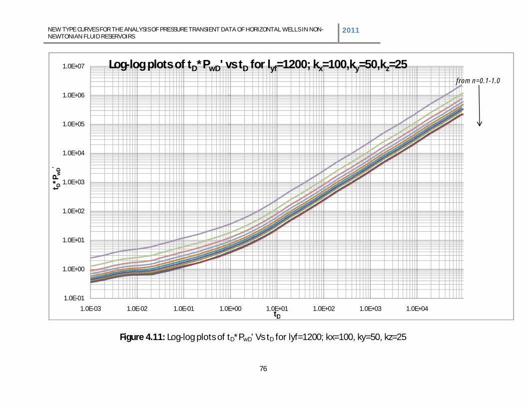
NEW TYPE CURVES FOR THE ANALYSIS OF PRESSURE TRANSIENT DATA OF HORIZONTAL WELLS IN NON-NEWTONIAN FLUID RESERVOIRS 2011
76
Figure 4.11: Log-log plots of tD*PwD' Vs tD for lyf=1200; kx=100, ky=50, kz=25
1.0E-01
1.0E+00
1.0E+01
1.0E+02
1.0E+03
1.0E+04
1.0E+05
1.0E+06
1.0E+07
1.0E-03 1.0E-02 1.0E-01 1.0E+00 1.0E+01 1.0E+02 1.0E+03 1.0E+04
t D*P
wD'
tD
Log-log plots of tD*PwD' vs tD for lyf=1200; kx=100,ky=50,kz=25from n=0.1-1.0
NEW TYPE CURVES FOR THE ANALYSIS OF PRESSURE TRANSIENT DATA OF HORIZONTAL WELLS IN NON-NEWTONIAN FLUID RESERVOIRS 2011
77
Figure 4.12: Log -Log Plot of PwD Vs tD for lyf=600ft; kx=ky=kz=75md
1.0E-01
1.0E+00
1.0E+01
1.0E+02
1.0E+03
1.0E+04
1.0E+05
1.0E+06
1.0E-03 1.0E-02 1.0E-01 1.0E+00 1.0E+01 1.0E+02 1.0E+03 1.0E+04
P wD
tD
Log -Log Plot of PwD Vs tD for lyf=600ft; kx=ky=kz=75md from n=0.1-1.0
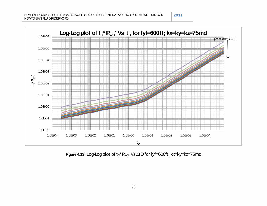
NEW TYPE CURVES FOR THE ANALYSIS OF PRESSURE TRANSIENT DATA OF HORIZONTAL WELLS IN NON-NEWTONIAN FLUID RESERVOIRS 2011
78
Figure 4.13: Log-Log plot of tD*PwD' Vs tD for lyf=600ft; kx=ky=kz=75md
1.0E-02
1.0E-01
1.0E+00
1.0E+01
1.0E+02
1.0E+03
1.0E+04
1.0E+05
1.0E+06
1.0E-04 1.0E-03 1.0E-02 1.0E-01 1.0E+00 1.0E+01 1.0E+02 1.0E+03 1.0E+04
t D*P
wD'
tD
Log-Log plot of tD*PwD' Vs tD for lyf=600ft; kx=ky=kz=75mdfrom n=0.1-1.0
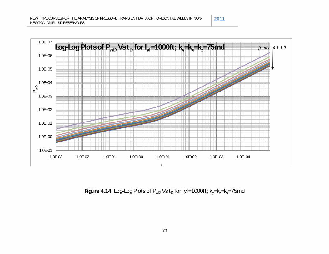
NEW TYPE CURVES FOR THE ANALYSIS OF PRESSURE TRANSIENT DATA OF HORIZONTAL WELLS IN NON-NEWTONIAN FLUID RESERVOIRS 2011
79
Figure 4.14: Log-Log Plots of PwD Vs tD for lyf=1000ft; ky=kx=kz=75md
1.0E-01
1.0E+00
1.0E+01
1.0E+02
1.0E+03
1.0E+04
1.0E+05
1.0E+06
1.0E+07
1.0E-03 1.0E-02 1.0E-01 1.0E+00 1.0E+01 1.0E+02 1.0E+03 1.0E+04
P wD
tD
Log-Log Plots of PwD Vs tD for lyf=1000ft; ky=kx=kz=75md from n=0.1-1.0
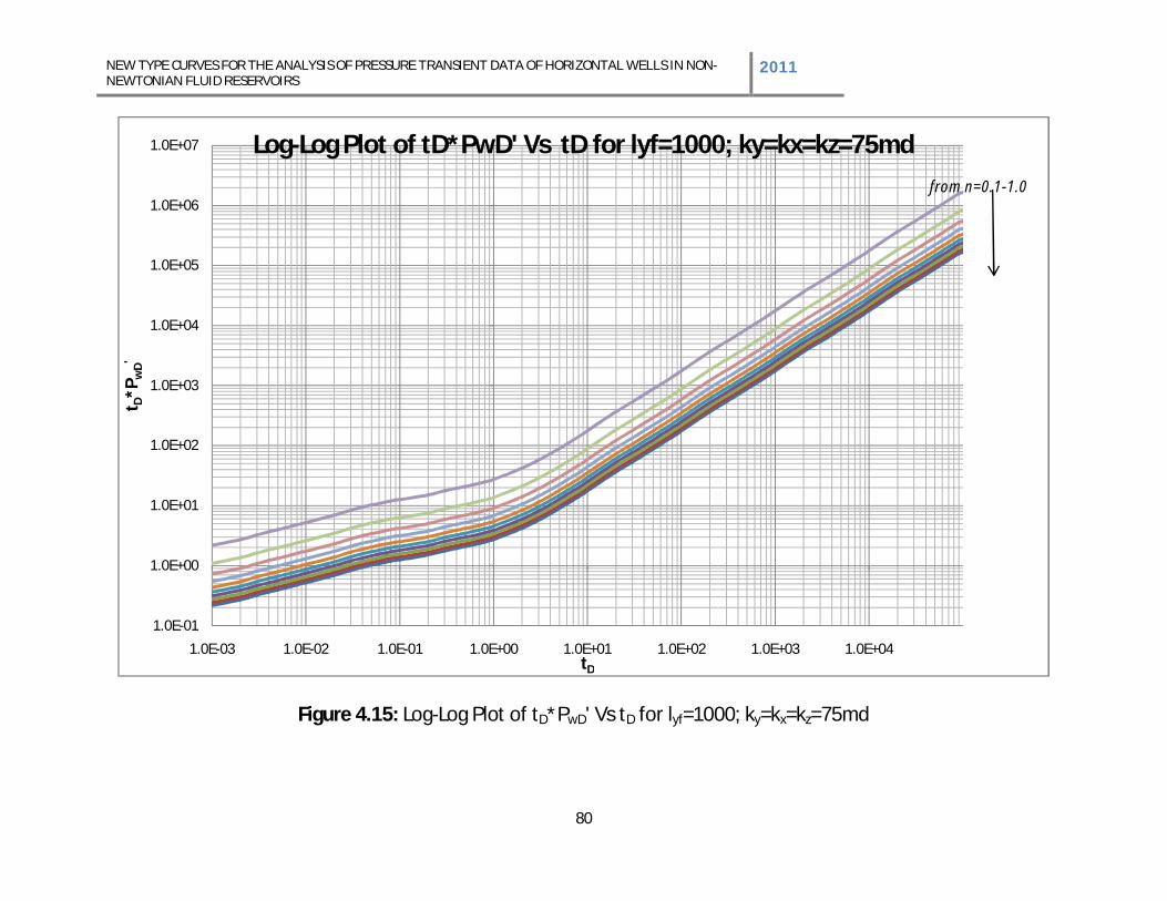
NEW TYPE CURVES FOR THE ANALYSIS OF PRESSURE TRANSIENT DATA OF HORIZONTAL WELLS IN NON-NEWTONIAN FLUID RESERVOIRS 2011
80
Figure 4.15: Log-Log Plot of tD*PwD' Vs tD for lyf=1000; ky=kx=kz=75md
1.0E-01
1.0E+00
1.0E+01
1.0E+02
1.0E+03
1.0E+04
1.0E+05
1.0E+06
1.0E+07
1.0E-03 1.0E-02 1.0E-01 1.0E+00 1.0E+01 1.0E+02 1.0E+03 1.0E+04
t D*P
wD'
tD
Log-Log Plot of tD*PwD' Vs tD for lyf=1000; ky=kx=kz=75md from n=0.1-1.0
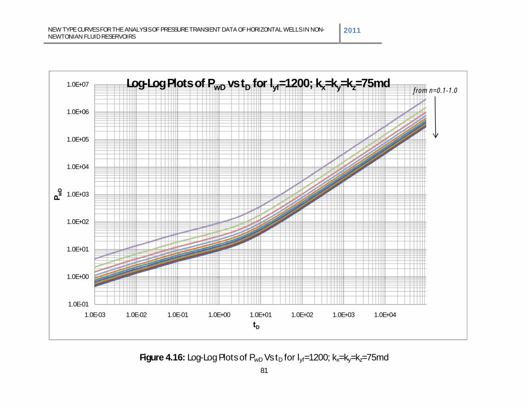
NEW TYPE CURVES FOR THE ANALYSIS OF PRESSURE TRANSIENT DATA OF HORIZONTAL WELLS IN NON-NEWTONIAN FLUID RESERVOIRS 2011
81
Figure 4.16: Log-Log Plots of PwD Vs tD for lyf=1200; kx=ky=kz=75md
1.0E-01
1.0E+00
1.0E+01
1.0E+02
1.0E+03
1.0E+04
1.0E+05
1.0E+06
1.0E+07
1.0E-03 1.0E-02 1.0E-01 1.0E+00 1.0E+01 1.0E+02 1.0E+03 1.0E+04
P wD
tD
Log-Log Plots of PwD vs tD for lyf=1200; kx=ky=kz=75mdfrom n=0.1-1.0
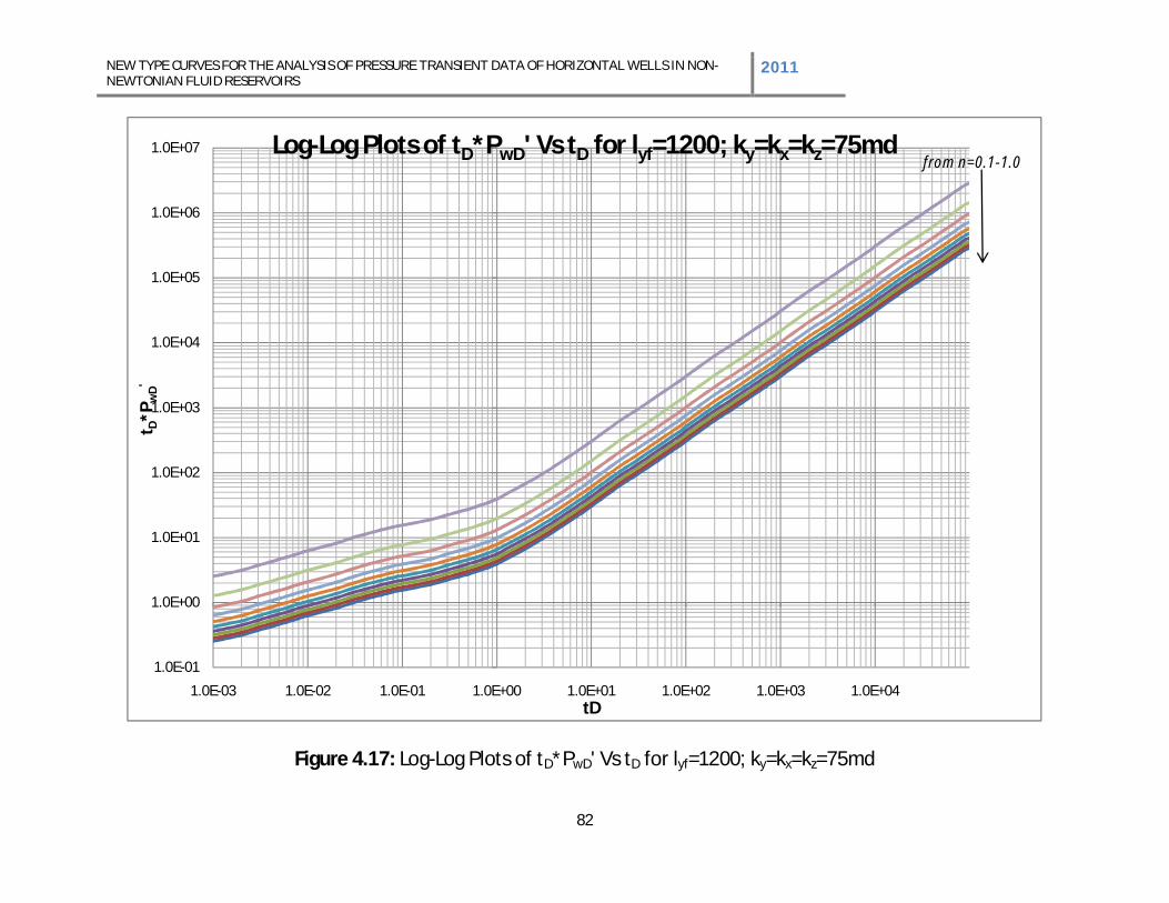
NEW TYPE CURVES FOR THE ANALYSIS OF PRESSURE TRANSIENT DATA OF HORIZONTAL WELLS IN NON-NEWTONIAN FLUID RESERVOIRS 2011
82
Figure 4.17: Log-Log Plots of tD*PwD' Vs tD for lyf=1200; ky=kx=kz=75md
1.0E-01
1.0E+00
1.0E+01
1.0E+02
1.0E+03
1.0E+04
1.0E+05
1.0E+06
1.0E+07
1.0E-03 1.0E-02 1.0E-01 1.0E+00 1.0E+01 1.0E+02 1.0E+03 1.0E+04
t D*P
wD'
tD
Log-Log Plots of tD*PwD' Vs tD for lyf=1200; ky=kx=kz=75mdfrom n=0.1-1.0
NEW TYPE CURVES FOR THE ANALYSIS OF PRESSURE TRANSIENT DATA OF HORIZONTAL WELLS IN NON-NEWTONIAN FLUID RESERVOIRS
2011
83
CHAPTER FIVE
5.0 CONCLUSIONS AND RECOMMENDATIONS
5.1 CONCLUSIONS
As the application of horizontal wells in enhanced oil recovery operations increases globally with
increased exploration and exploitation of heavy crude in places like Venezuela, Canada etc, the
following conclusions were made from this study;
The finite-difference Numerical solution of the partial differential equation as developed in
this study describing the flow of non-Newtonian fluid in a reservoir with permeability
heterogeneity is valid to a large degree of accuracy. This is because close value of reservoir
properties where obtained in the validation when a Newtonian reservoir fluid is considered.
The pressure drop in the draw-down of a non-Newtonian fluid reservoir is higher compared to
the pressure drop in a Newtonian fluid reservoir.
In cases when the horizontal well length is 600ft in an heterogeneous reservoir, early linear,
Pseudo radial , a transition flow regime and Pseudo steady state flow were observed which
aided the determination of reservoir properties such as;
,
As the horizontal well length increases the type curve indicates the absence of the
psedoradial radial flow. A very short linear alongside Pseudo steady state flow regime is
observed.
In the analysis of the pressure transient, the correlation factor obtained in the study of
Vongvuthiopornchai and Raghavan, 1987 were found to be applicable and valid for the
different values of n
For cases where the reservoir is homogeneous with respect to permeability and porosity, the
early flow regime is not seen irrespective of the horizontal well length.

NEW TYPE CURVES FOR THE ANALYSIS OF PRESSURE TRANSIENT DATA OF HORIZONTAL WELLS IN NON-NEWTONIAN FLUID RESERVOIRS 2011
84
The novel approach for the analysis of pressure transient data of horizontal well in non-
Newtonian reservoir fluids as presented in this work is found to be consistent with the result
obtained in the works of Igbokoyi and Tiab,2007;
The pressure derivative method can only be used to obtain average permeability when the
radial flow exists.
5.2 RECOMMENDATIONS
In order to perfect the study made in this work, the following recommendations are made;
Further works should consider the effect of skin and wellbore storage in the analysis
of pressure transient data of horizontal well in non-Newtonian fluid reservoirs
Much finer grids size should be used in any further study; this will require a high
performance computer which was not used in this study.
Other numerical method such as finite element method should be used to solve the
partial differential equation describing the flow of non-Newtonian fluid in porous
media. This will enable the modeling of reservoirs of different geometry or shape and
reduce errors due to approximation as encountered when finite difference is used.
Considering the fact that multiphase conditions exist in the reservoir, a study on the
multiphase flow of non-Newtonian fluid in the reservoir should be a right step
Further works should look into the analysis of horizontal well in non-Newtonian fluids
considering a 3 dimensional radial flow.
Further works on this subject matter should consider local grid refinement throughout
the length of the horizontal well to improve on the results obtained.
The application of this work to the characterization of heavy oil reservoirs should also
be looked into by subsequent studies.
NEW TYPE CURVES FOR THE ANALYSIS OF PRESSURE TRANSIENT DATA OF HORIZONTAL WELLS IN NON-NEWTONIAN FLUID RESERVOIRS 2011
85
REFERENCES
Adam T.Bourgoyne Jr.,Keith K. Millheim, Martin E. Chenevert, F.S. Young Jr: ‘Applied Drilling Engineering’ first printing Society of Petroleum Engineers Richardson TX,1986
A. S. Odeh and H. T. Yang: ‘Flow of Non-Newtonian Power-Law Fluids through Porous Media’ April, 1979 (SPE 7150)
Alpheus O. Igbokoyi and Djebbar Tiab, SPE, U. of Oklahoma: ‘New Type Curves for the Analysis of Pressure Transient Data Dominated by Skin and Wellbore Storage-Non-Newtonian Fluid’ April, 2007. (SPE 106997)
Aziz S. Odeh and D.K Babu: Transient Flow behavior of Horizontal Wells: Pressure Drawdown and Buildup Analysis. SPE Formation Evaluation, March 1990.
Aziz, K and Settari, A.: Petroleum Reservoir Simulation, Applied Science Publishers Ltd., London (1979) 69-92.
Bird, B. R., Stewart, W. E and Lightfoot, E.N.: Transport Phenomena, John Wiley and Sons Inc. New York City (1960) 206
Chi U. Ikoku, University of Tulsa; ‘Practical Application of Non-Newtonian Transient Flow Analysis’ SPE Las Vegas, 1979 (SPE 8351)
Christopher, R. H. and Middleman, S.: ‘Power-Law Flow Through a Packed Tube,’ Ind & Eng. Chem. Fund. (Nov. 1965) 4, No. 4 422-426
Chi U. Ikoku and Henry J. Ramey; ‘Wellbore Storage and Skin Effects during the Transient Flow of Non-Newtonian Power-Law fluids in Porous Media’ February, 1980 (SPE 7449)
D. K. Babu, G.B. Asher, A.S. Odeh: ’A Reliable Method for Analyzing Constant-Rate Drawdown Data From a Horizontal well’. SPE, 1992 (SPE 02450)
Engler, T. and Tiab, D.: ‘Analysis of Pressure and pressure derivative without tpe curve matching, for Naturally fractured reservoirs’ Journal of Petroleum Science and Engineering, Nov, 1995.
F. Medeiros Jr., E. Ozkan and H. Kazemi: ‘A Semianalytical Approach to Model Pressure Transient in Heterogeneous Reservoirs’ April, 2010 SPE Reservoir Evaluation and Engineering. (SPE 102834)
Gencer, S and Ikoku, C. U.: ‘Well Test Analysis for Two –Phase Flow of Non-Newtonian Power-law and Newtonian Fluids,’ J. Energy Resources Tech. (June 1984) 106,295-305.
NEW TYPE CURVES FOR THE ANALYSIS OF PRESSURE TRANSIENT DATA OF HORIZONTAL WELLS IN NON-NEWTONIAN FLUID RESERVOIRS 2011
86
Ikoku, C.U and Ramey, H. J .Jr; ‘Transient Flow of Non-Newtonian Power-Law Fluids in Porous Media’ January, 1979 (SPE 7139)
Irina Katime-Meindl and Djebbar Tiab; ‘Analysis of Pressure Transient Test of Non-Newtonian Fluids in Infinite Reservoir and in the Presence of a single linear Boundary by the Direct Synthesis Technique’ September, 2001 (SPE 71587)
Joseph S. Olarewaju: ‘A Reservoir Model of Non-Newtonian Fluid Flow. SPE, Tulsa Oklahoma, June 1992’ (SPE 25301)
M. B. Issaka and A.K Ambastha.: ‘Drawdown and Buildup Pressure Derivative Analyses for Horizontal wells’ paper SPE 24323 presented at the SPE Rocky Mountain Regional Meeting, Wyoming. May, 1992.
M.D. Clonts and H.J Ramey.: ‘Pressure Transient Analysis for wells with Horizontal Drainholes’ paper SPE 15116 presented at the 56th California Regional meeting of SPE CA. April, 1966.
McDonald, A.E.: Approximate Solutions for Flow of Non-Newtonian Power-Law Fluids Through Porous Media,’ Paper SPE 7690 Presented at the 1979 SPE Reservoir simulation symposium, Denver, Feb
Micheal J. Economides, Franz X. Delmbacher, Clemens W. Brand and Zoltan E. Heinemann: ‘Comprehensive Simulation of Horizontal-well Performance’, SPE Formation Evaluation, December 1991 (SPE 20717)
M.Y. Soliman, J.Ansah, J.Burris, S. Stephenson, M. Proett: ‘Well Test Analysis in the New Economy’, July, 2003, Volume 42, No.7 Journal of Canadian Petroleum Technology.
Murtha, J. A. and Ertekin, T.: ‘Numerical Simulation of Power-law Fluid Flow in Vertically Fractured Reservoir,’ paper SPE 12011 presented at the 1983 SPE Annual Technical Conference and Exhibitiob, San Francisco.
N. Al-Mohannadi, E. Ozkan and H. Kazemi; ‘Grid-System requirements in Numerical Modeling of Pressure-Transient Tests in Horizontal Wells’ February, 2007 (SPE 92041)
O. Lund and Chi U. Ikoku; ‘Pressure Transient Behavior of Non-Newtonian/ Newtonian Fluid Composite Reservoirs’ April, 1981 (SPE 9401)
P.A. Goode and R.K.M. Thambynayagam: ‘Pressure Drawdown and Buildup Analysis of Horizontal Wells in Anisotropic Media’ SPE Formation Evaluation, December 1987. (SPE 14250)
Puthigai, S.K and Tiab, D,: ‘Application of Function of vertically Fractured Wells-Field Cases’ paper SPE 11028 presented at the 1982 SPE Annual Technical Conference and Exhibition, New Orleans, Sept. 26-29
S. Al Rbeawi and D. Tiab.: ‘Pressure Transient Analysis of Horizontal wells in a Multi-Boundary System’ paper SPE 142316, Present at the SPE Production and Operations Symposium held in Oklahoma March,2011
Savins, J.G.: ‘Non-Newtonian Flow through Porous Media’ Ind. & Eng. Chem. (oct. 1969) 61. N0. 10, 18-47.
NEW TYPE CURVES FOR THE ANALYSIS OF PRESSURE TRANSIENT DATA OF HORIZONTAL WELLS IN NON-NEWTONIAN FLUID RESERVOIRS 2011
87
S. Vongvuthipornchai and R. Raghavan: ‘Pressure Falloff Behavior in Vertically Fractured Wells: Non-Newtonian Power-Law Fluids’ SPE Formation Evaluation, December 1987. (SPE 13058)
S. Vongvuthipornchai and Rajagopal Raghavan; ‘well test Analysis of Data Dominated by Storage and Skin: Non-Newtonian Power-Law Fluids’ December, 1987 (SPE 14454)
Tiab, D.: ‘Analysis of Pressure and Pressure derivative without type curve matching- Skin and wellbore storage’ Journal of Petroleum Science and Engineering. Nov, 1994.
Turgay Ertekin, Jamal H. Abou-Kassem and Gregory R. king: ‘Basic Applied Reservoir Simulation’, SPE, 2001
T. Ertekin, O. Cicek and M.A. Adequmi,’ Pennsylvania State U. and M.E. Daud, Petronas: Pressure Transient Behavior of Non-Newtonian/Newtonian Fluid Composite Systems in porous Media with a Finite Conductivity Vertical Fracture’ SPE pittsburrgh, Pennsylvania, 1987 (SPE 17053)
Van Poollen, H.K and Jargon, J. R: ‘Steady-State and Unsteady-State Flow of Non-Newtonian Fluids through Porous Media’ Society of Petroleum Engineering Journal, 1969, 80-88 (SPE 1567)
V.R Penmatcha and Khalid Aziz: ‘Comprehensive Reservoir/Wellbore Model for Horizontal Wells’, SPE Journal September, 1999 (SPE 571942)
Wong, D. W., Harrington, A.G., and Cinco-L., H.; ‘Application of the Pressure Derivative Function in the Pressure Transient Testing of Fractured Wells,’ paper SPE 13056 presented at the 1984 SPE Annual Technical Conference and Exhibition, Houston, Sept. 16-19.

NEW TYPE CURVES FOR THE ANALYSIS OF PRESSURE TRANSIENT DATA OF HORIZONTAL WELLS IN NON-NEWTONIAN FLUID RESERVOIRS 2011
88
NOMENCLATURE
=
=
=
= . .
= . .
=
= . .
= / /
=
= /
=
= /
=
=
=
= /
= , /
= . .
= ,
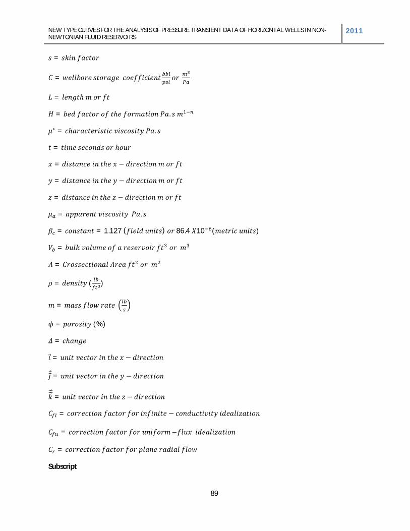
NEW TYPE CURVES FOR THE ANALYSIS OF PRESSURE TRANSIENT DATA OF HORIZONTAL WELLS IN NON-NEWTONIAN FLUID RESERVOIRS 2011
89
=
=
=
= .
= .
=
=
=
=
= .
= = 1.127 ( ) 86.4 10 ( )
=
=
= ( )
=
= (%)
=
=
=
=
=
= –
=
Subscript

NEW TYPE CURVES FOR THE ANALYSIS OF PRESSURE TRANSIENT DATA OF HORIZONTAL WELLS IN NON-NEWTONIAN FLUID RESERVOIRS 2011
90
=
=
, , =
=
=
=
=
=
=
=
=
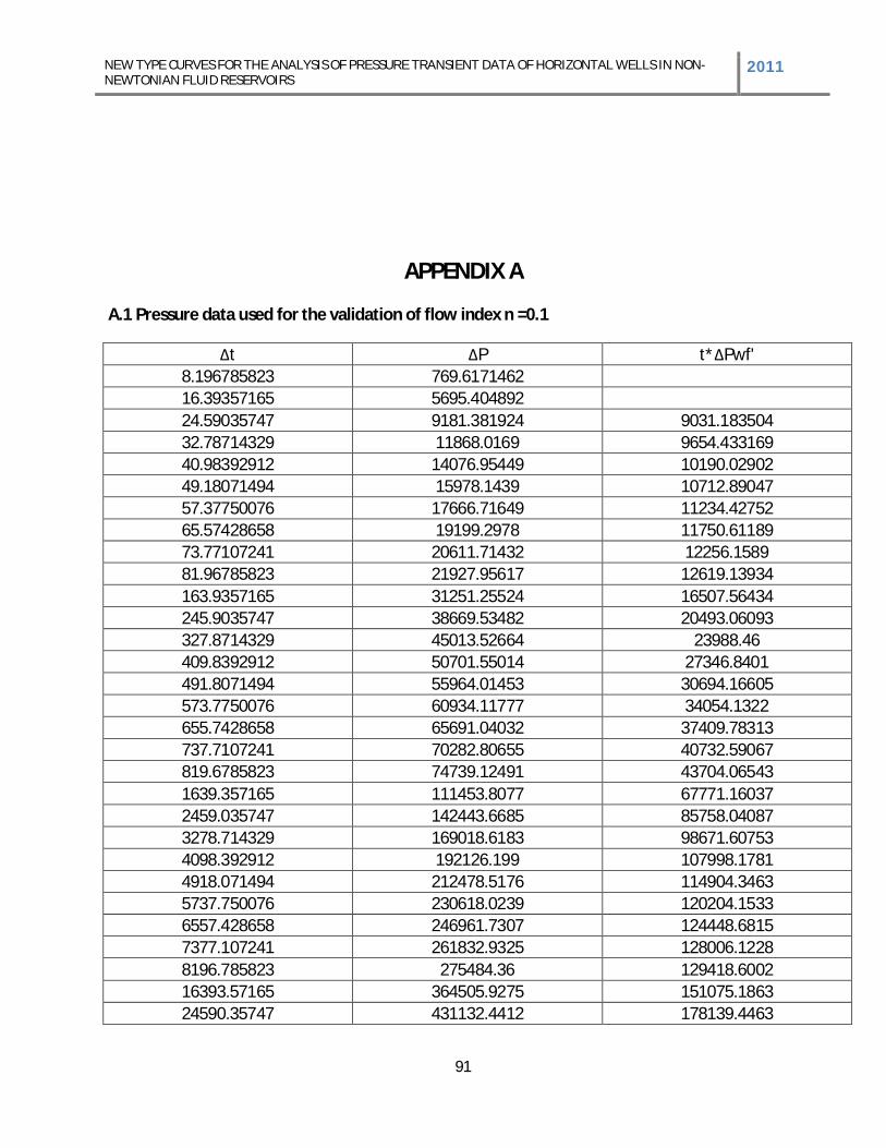
NEW TYPE CURVES FOR THE ANALYSIS OF PRESSURE TRANSIENT DATA OF HORIZONTAL WELLS IN NON-NEWTONIAN FLUID RESERVOIRS 2011
91
APPENDIX A
A.1 Pressure data used for the validation of flow index n =0.1
t P t* Pwf' 8.196785823 769.6171462 16.39357165 5695.404892 24.59035747 9181.381924 9031.183504 32.78714329 11868.0169 9654.433169 40.98392912 14076.95449 10190.02902 49.18071494 15978.1439 10712.89047 57.37750076 17666.71649 11234.42752 65.57428658 19199.2978 11750.61189 73.77107241 20611.71432 12256.1589 81.96785823 21927.95617 12619.13934 163.9357165 31251.25524 16507.56434 245.9035747 38669.53482 20493.06093 327.8714329 45013.52664 23988.46 409.8392912 50701.55014 27346.8401 491.8071494 55964.01453 30694.16605 573.7750076 60934.11777 34054.1322 655.7428658 65691.04032 37409.78313 737.7107241 70282.80655 40732.59067 819.6785823 74739.12491 43704.06543 1639.357165 111453.8077 67771.16037 2459.035747 142443.6685 85758.04087 3278.714329 169018.6183 98671.60753 4098.392912 192126.199 107998.1781 4918.071494 212478.5176 114904.3463 5737.750076 230618.0239 120204.1533 6557.428658 246961.7307 124448.6815 7377.107241 261832.9325 128006.1228 8196.785823 275484.36 129418.6002 16393.57165 364505.9275 151075.1863 24590.35747 431132.4412 178139.4463
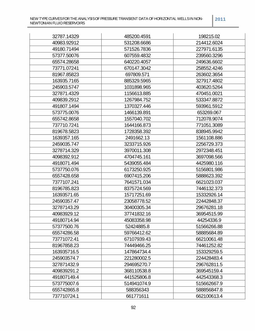
NEW TYPE CURVES FOR THE ANALYSIS OF PRESSURE TRANSIENT DATA OF HORIZONTAL WELLS IN NON-NEWTONIAN FLUID RESERVOIRS 2011
92
32787.14329 485200.4591 198215.02 40983.92912 531208.6686 214412.6024 49180.71494 571526.7836 227971.6135 57377.50076 607559.4832 239560.3296 65574.28658 640220.4057 249636.6602 73771.07241 670147.3042 258552.4246 81967.85823 697809.571 263602.3654 163935.7165 885329.5965 327917.4802 245903.5747 1031898.965 403620.5264 327871.4329 1156613.885 470451.0021 409839.2912 1267984.752 533347.8872 491807.1494 1370327.446 593961.5912 573775.0076 1466139.891 653269.067 655742.8658 1557040.702 712078.9074 737710.7241 1644166.873 771051.3089 819678.5823 1728358.392 838945.9942 1639357.165 2491662.13 1561108.886 2459035.747 3233715.926 2256729.373 3278714.329 3970011.308 2972348.451 4098392.912 4704745.161 3697098.566 4918071.494 5439055.484 4425980.116 5737750.076 6173250.925 5156801.986 6557428.658 6907415.206 5888623.392 7377107.241 7641571.034 6621023.037 8196785.823 8375724.569 7446132.373 16393571.65 15717251.69 15332926.14 24590357.47 23058778.52 22442848.37 32787143.29 30400305.34 29676281.18 40983929.12 37741832.16 36954515.99 49180714.94 45083358.98 44254336.9 57377500.76 52424885.8 51566266.88 65574286.58 59766412.62 58885684.89 73771072.41 67107939.43 66210061.48 81967858.23 74449466.25 74461252.82 163935716.5 147864734.4 153329259.5 245903574.7 221280002.5 224428483.4 327871432.9 294695270.7 296762811.5 409839291.2 368110538.8 369545159.4 491807149.4 441525806.8 442543368.3 573775007.6 514941074.9 515662667.9 655742865.8 588356343 588856847.8 737710724.1 661771611 662100613.4
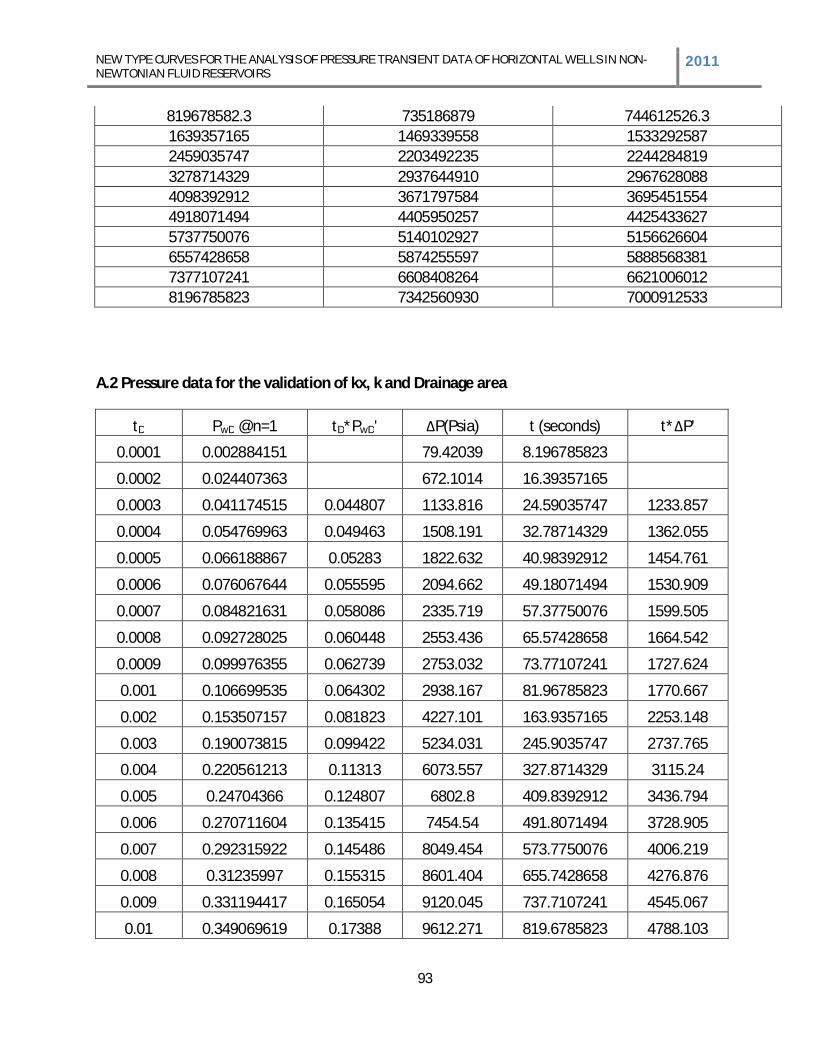
NEW TYPE CURVES FOR THE ANALYSIS OF PRESSURE TRANSIENT DATA OF HORIZONTAL WELLS IN NON-NEWTONIAN FLUID RESERVOIRS 2011
93
819678582.3 735186879 744612526.3 1639357165 1469339558 1533292587 2459035747 2203492235 2244284819 3278714329 2937644910 2967628088 4098392912 3671797584 3695451554 4918071494 4405950257 4425433627 5737750076 5140102927 5156626604 6557428658 5874255597 5888568381 7377107241 6608408264 6621006012 8196785823 7342560930 7000912533
A.2 Pressure data for the validation of kx, k and Drainage area
tD PwD @n=1 tD*PwD' P(Psia) t (seconds) t* P'
0.0001 0.002884151 79.42039 8.196785823
0.0002 0.024407363 672.1014 16.39357165
0.0003 0.041174515 0.044807 1133.816 24.59035747 1233.857
0.0004 0.054769963 0.049463 1508.191 32.78714329 1362.055
0.0005 0.066188867 0.05283 1822.632 40.98392912 1454.761
0.0006 0.076067644 0.055595 2094.662 49.18071494 1530.909
0.0007 0.084821631 0.058086 2335.719 57.37750076 1599.505
0.0008 0.092728025 0.060448 2553.436 65.57428658 1664.542
0.0009 0.099976355 0.062739 2753.032 73.77107241 1727.624
0.001 0.106699535 0.064302 2938.167 81.96785823 1770.667
0.002 0.153507157 0.081823 4227.101 163.9357165 2253.148
0.003 0.190073815 0.099422 5234.031 245.9035747 2737.765
0.004 0.220561213 0.11313 6073.557 327.8714329 3115.24
0.005 0.24704366 0.124807 6802.8 409.8392912 3436.794
0.006 0.270711604 0.135415 7454.54 491.8071494 3728.905
0.007 0.292315922 0.145486 8049.454 573.7750076 4006.219
0.008 0.31235997 0.155315 8601.404 655.7428658 4276.876
0.009 0.331194417 0.165054 9120.045 737.7107241 4545.067
0.01 0.349069619 0.17388 9612.271 819.6785823 4788.103
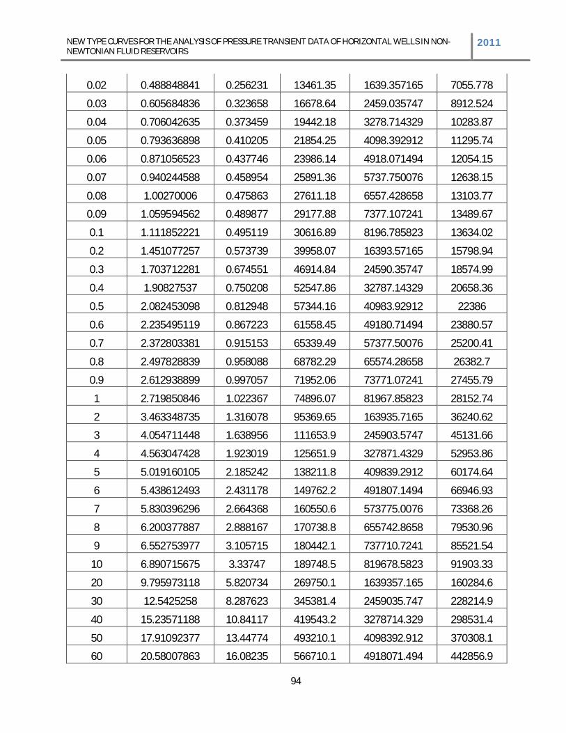
NEW TYPE CURVES FOR THE ANALYSIS OF PRESSURE TRANSIENT DATA OF HORIZONTAL WELLS IN NON-NEWTONIAN FLUID RESERVOIRS 2011
94
0.02 0.488848841 0.256231 13461.35 1639.357165 7055.778
0.03 0.605684836 0.323658 16678.64 2459.035747 8912.524
0.04 0.706042635 0.373459 19442.18 3278.714329 10283.87
0.05 0.793636898 0.410205 21854.25 4098.392912 11295.74
0.06 0.871056523 0.437746 23986.14 4918.071494 12054.15
0.07 0.940244588 0.458954 25891.36 5737.750076 12638.15
0.08 1.00270006 0.475863 27611.18 6557.428658 13103.77
0.09 1.059594562 0.489877 29177.88 7377.107241 13489.67
0.1 1.111852221 0.495119 30616.89 8196.785823 13634.02
0.2 1.451077257 0.573739 39958.07 16393.57165 15798.94
0.3 1.703712281 0.674551 46914.84 24590.35747 18574.99
0.4 1.90827537 0.750208 52547.86 32787.14329 20658.36
0.5 2.082453098 0.812948 57344.16 40983.92912 22386
0.6 2.235495119 0.867223 61558.45 49180.71494 23880.57
0.7 2.372803381 0.915153 65339.49 57377.50076 25200.41
0.8 2.497828839 0.958088 68782.29 65574.28658 26382.7
0.9 2.612938899 0.997057 71952.06 73771.07241 27455.79
1 2.719850846 1.022367 74896.07 81967.85823 28152.74
2 3.463348735 1.316078 95369.65 163935.7165 36240.62
3 4.054711448 1.638956 111653.9 245903.5747 45131.66
4 4.563047428 1.923019 125651.9 327871.4329 52953.86
5 5.019160105 2.185242 138211.8 409839.2912 60174.64
6 5.438612493 2.431178 149762.2 491807.1494 66946.93
7 5.830396296 2.664368 160550.6 573775.0076 73368.26
8 6.200377887 2.888167 170738.8 655742.8658 79530.96
9 6.552753977 3.105715 180442.1 737710.7241 85521.54
10 6.890715675 3.33747 189748.5 819678.5823 91903.33
20 9.795973118 5.820734 269750.1 1639357.165 160284.6
30 12.5425258 8.287623 345381.4 2459035.747 228214.9
40 15.23571188 10.84117 419543.2 3278714.329 298531.4
50 17.91092377 13.44774 493210.1 4098392.912 370308.1
60 20.58007863 16.08235 566710.1 4918071.494 442856.9
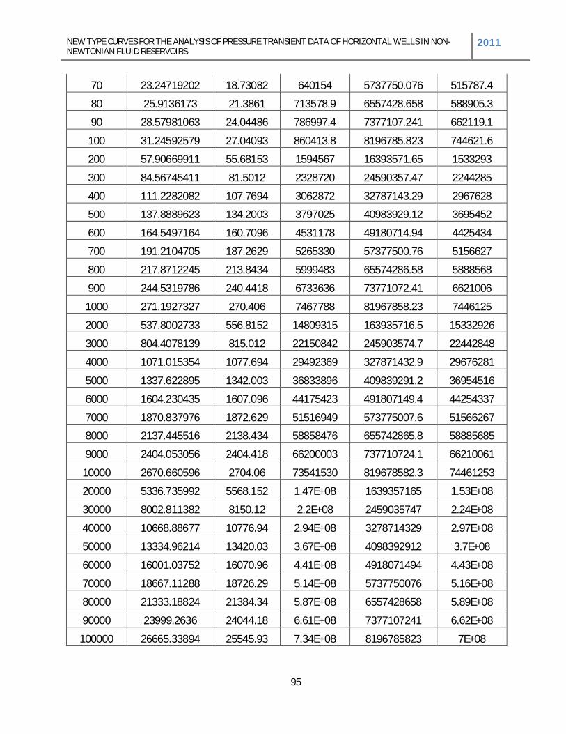
NEW TYPE CURVES FOR THE ANALYSIS OF PRESSURE TRANSIENT DATA OF HORIZONTAL WELLS IN NON-NEWTONIAN FLUID RESERVOIRS 2011
95
70 23.24719202 18.73082 640154 5737750.076 515787.4
80 25.9136173 21.3861 713578.9 6557428.658 588905.3
90 28.57981063 24.04486 786997.4 7377107.241 662119.1
100 31.24592579 27.04093 860413.8 8196785.823 744621.6
200 57.90669911 55.68153 1594567 16393571.65 1533293
300 84.56745411 81.5012 2328720 24590357.47 2244285
400 111.2282082 107.7694 3062872 32787143.29 2967628
500 137.8889623 134.2003 3797025 40983929.12 3695452
600 164.5497164 160.7096 4531178 49180714.94 4425434
700 191.2104705 187.2629 5265330 57377500.76 5156627
800 217.8712245 213.8434 5999483 65574286.58 5888568
900 244.5319786 240.4418 6733636 73771072.41 6621006
1000 271.1927327 270.406 7467788 81967858.23 7446125
2000 537.8002733 556.8152 14809315 163935716.5 15332926
3000 804.4078139 815.012 22150842 245903574.7 22442848
4000 1071.015354 1077.694 29492369 327871432.9 29676281
5000 1337.622895 1342.003 36833896 409839291.2 36954516
6000 1604.230435 1607.096 44175423 491807149.4 44254337
7000 1870.837976 1872.629 51516949 573775007.6 51566267
8000 2137.445516 2138.434 58858476 655742865.8 58885685
9000 2404.053056 2404.418 66200003 737710724.1 66210061
10000 2670.660596 2704.06 73541530 819678582.3 74461253
20000 5336.735992 5568.152 1.47E+08 1639357165 1.53E+08
30000 8002.811382 8150.12 2.2E+08 2459035747 2.24E+08
40000 10668.88677 10776.94 2.94E+08 3278714329 2.97E+08
50000 13334.96214 13420.03 3.67E+08 4098392912 3.7E+08
60000 16001.03752 16070.96 4.41E+08 4918071494 4.43E+08
70000 18667.11288 18726.29 5.14E+08 5737750076 5.16E+08
80000 21333.18824 21384.34 5.87E+08 6557428658 5.89E+08
90000 23999.2636 24044.18 6.61E+08 7377107241 6.62E+08
100000 26665.33894 25545.93 7.34E+08 8196785823 7E+08
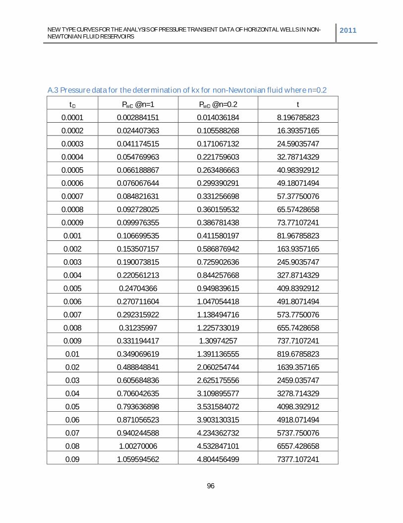
NEW TYPE CURVES FOR THE ANALYSIS OF PRESSURE TRANSIENT DATA OF HORIZONTAL WELLS IN NON-NEWTONIAN FLUID RESERVOIRS 2011
96
A.3 Pressure data for the determination of kx for non-Newtonian fluid where n=0.2
tD PwD @n=1 PwD @n=0.2 t
0.0001 0.002884151 0.014036184 8.196785823
0.0002 0.024407363 0.105588268 16.39357165
0.0003 0.041174515 0.171067132 24.59035747
0.0004 0.054769963 0.221759603 32.78714329
0.0005 0.066188867 0.263486663 40.98392912
0.0006 0.076067644 0.299390291 49.18071494
0.0007 0.084821631 0.331256698 57.37750076
0.0008 0.092728025 0.360159532 65.57428658
0.0009 0.099976355 0.386781438 73.77107241
0.001 0.106699535 0.411580197 81.96785823
0.002 0.153507157 0.586876942 163.9357165
0.003 0.190073815 0.725902636 245.9035747
0.004 0.220561213 0.844257668 327.8714329
0.005 0.24704366 0.949839615 409.8392912
0.006 0.270711604 1.047054418 491.8071494
0.007 0.292315922 1.138494716 573.7750076
0.008 0.31235997 1.225733019 655.7428658
0.009 0.331194417 1.30974257 737.7107241
0.01 0.349069619 1.391136555 819.6785823
0.02 0.488848841 2.060254744 1639.357165
0.03 0.605684836 2.625175556 2459.035747
0.04 0.706042635 3.109895577 3278.714329
0.05 0.793636898 3.531584072 4098.392912
0.06 0.871056523 3.903130315 4918.071494
0.07 0.940244588 4.234362732 5737.750076
0.08 1.00270006 4.532847101 6557.428658
0.09 1.059594562 4.804456499 7377.107241
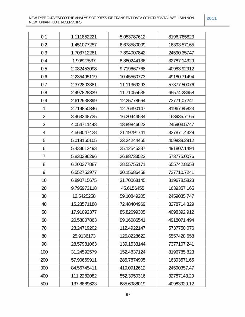
NEW TYPE CURVES FOR THE ANALYSIS OF PRESSURE TRANSIENT DATA OF HORIZONTAL WELLS IN NON-NEWTONIAN FLUID RESERVOIRS 2011
97
0.1 1.111852221 5.053787612 8196.785823
0.2 1.451077257 6.678580009 16393.57165
0.3 1.703712281 7.894007842 24590.35747
0.4 1.90827537 8.880244136 32787.14329
0.5 2.082453098 9.719667768 40983.92912
0.6 2.235495119 10.45560773 49180.71494
0.7 2.372803381 11.11369293 57377.50076
0.8 2.497828839 11.71055635 65574.28658
0.9 2.612938899 12.25778664 73771.07241
1 2.719850846 12.76390147 81967.85823
2 3.463348735 16.20444534 163935.7165
3 4.054711448 18.89846623 245903.5747
4 4.563047428 21.19291741 327871.4329
5 5.019160105 23.24244465 409839.2912
6 5.438612493 25.12545337 491807.1494
7 5.830396296 26.88733522 573775.0076
8 6.200377887 28.55755171 655742.8658
9 6.552753977 30.15686458 737710.7241
10 6.890715675 31.70068145 819678.5823
20 9.795973118 45.6156455 1639357.165
30 12.5425258 59.10849205 2459035.747
40 15.23571188 72.48404969 3278714.329
50 17.91092377 85.82699305 4098392.912
60 20.58007863 99.16086541 4918071.494
70 23.24719202 112.4922147 5737750.076
80 25.9136173 125.8228622 6557428.658
90 28.57981063 139.1533144 7377107.241
100 31.24592579 152.4837124 8196785.823
200 57.90669911 285.7874905 16393571.65
300 84.56745411 419.0912612 24590357.47
400 111.2282082 552.3950316 32787143.29
500 137.8889623 685.6988019 40983929.12
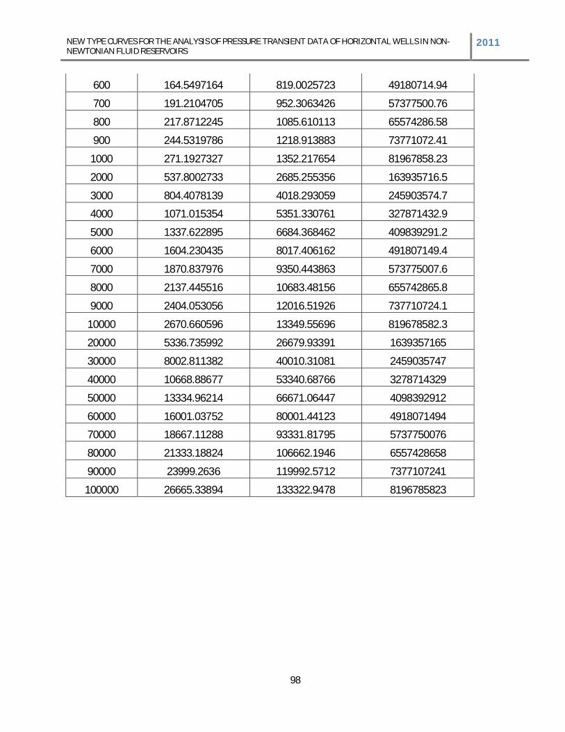
NEW TYPE CURVES FOR THE ANALYSIS OF PRESSURE TRANSIENT DATA OF HORIZONTAL WELLS IN NON-NEWTONIAN FLUID RESERVOIRS 2011
98
600 164.5497164 819.0025723 49180714.94
700 191.2104705 952.3063426 57377500.76
800 217.8712245 1085.610113 65574286.58
900 244.5319786 1218.913883 73771072.41
1000 271.1927327 1352.217654 81967858.23
2000 537.8002733 2685.255356 163935716.5
3000 804.4078139 4018.293059 245903574.7
4000 1071.015354 5351.330761 327871432.9
5000 1337.622895 6684.368462 409839291.2
6000 1604.230435 8017.406162 491807149.4
7000 1870.837976 9350.443863 573775007.6
8000 2137.445516 10683.48156 655742865.8
9000 2404.053056 12016.51926 737710724.1
10000 2670.660596 13349.55696 819678582.3
20000 5336.735992 26679.93391 1639357165
30000 8002.811382 40010.31081 2459035747
40000 10668.88677 53340.68766 3278714329
50000 13334.96214 66671.06447 4098392912
60000 16001.03752 80001.44123 4918071494
70000 18667.11288 93331.81795 5737750076
80000 21333.18824 106662.1946 6557428658
90000 23999.2636 119992.5712 7377107241
100000 26665.33894 133322.9478 8196785823
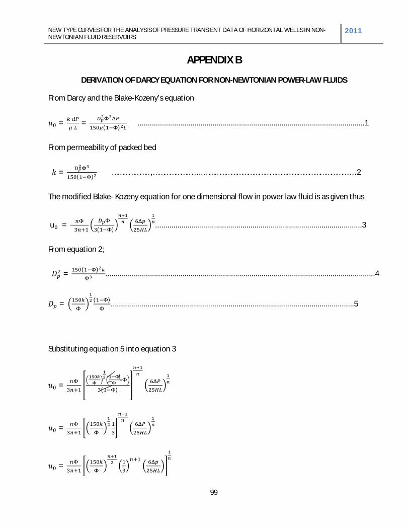
NEW TYPE CURVES FOR THE ANALYSIS OF PRESSURE TRANSIENT DATA OF HORIZONTAL WELLS IN NON-NEWTONIAN FLUID RESERVOIRS 2011
99
APPENDIX B
DERIVATION OF DARCY EQUATION FOR NON-NEWTONIAN POWER-LAW FLUIDS
From Darcy and the Blake-Kozeny’s equation
=
=( )
................................................................................................................1
From permeability of packed bed
=( )
…………………,……………………...…………………………………………………………………….….2
The modified Blake- Kozeny equation for one dimensional flow in power law fluid is as given thus
u = ( )
......................................................................................................3
From equation 2;
= ( ) .....................................................................................................................................4
= ( )........................................................................................................................5
Substituting equation 5 into equation 3
=( )
=
=
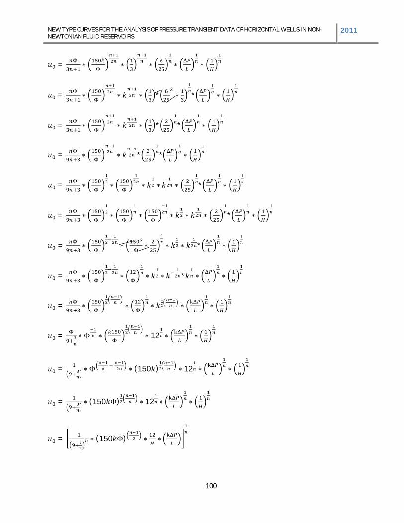
NEW TYPE CURVES FOR THE ANALYSIS OF PRESSURE TRANSIENT DATA OF HORIZONTAL WELLS IN NON-NEWTONIAN FLUID RESERVOIRS 2011
100
=
= * *
= * *
= * *
= *
= *
= *
= *
=
= 12
= (150 ) 12
= (150 ) 12
= (150 )
NEW TYPE CURVES FOR THE ANALYSIS OF PRESSURE TRANSIENT DATA OF HORIZONTAL WELLS IN NON-NEWTONIAN FLUID RESERVOIRS 2011
101
=( )
= 9 + (150 )
= 9 + (150 ) 12
=( )
........................................................................................................6
Comparing equation 6 with the Darcy’s equation,
( )
Thus, equation 6 can be re-written as;
.............................................................................................................................7