New technique for ensemble dressing combining Multimodel SuperEnsemble and precipitation PDF

EMS/ECAM Toulouse, 29/09/2009 D. Cane M. Milelli 1

New technique for ensemble dressing combiningMultimodel SuperEnsemble and precipitation PDFNew technique for ensemble dressing combiningMultimodel SuperEnsemble and precipitation PDF

9th EMS Annual Meeting/9th European Conference on Applications of Meteorology

Toulouse,29/09/2009

Daniele CaneMassimo Milelli


Outlook

• Multimodel SuperEnsemble dressing • Precipitation PDF• Weight calculation• Probabilistic forecast statistics • Results• Conclusions• Work in progress


Multimodel SuperEnsemble dressing

PROBABILISTIC QPF:

• Operational weather forecast support

• Better knowledge of the precipitation field characteristics

• Propagation of the probabilistic distribution to the hydrological chain: probabilistic discharge calculations

OUR PROPOSAL:

• Evaluation of the observed PDF conditioned to the model forecasts

• Combination of the PDFs with the Multimodel SuperEnsemble weight calculation technique

probabilistic Multimodel SuperEnsemble dressing



We associate to each model’s QPF the empirical Probability Density Function (PDF) and we calculate the (weighted) mean PDF.

Weights are evaluated with the Multimodel SuperEnsemble technique.

Example:

model1 -> 0 mm

model2 -> 5 mm

model3 -> 13 mm

model4 -> 16 mm

0 5 13 16

0.0001

0.001

0.01

0.1

1

0 10 20 30 40 50

precipitation (mm)

freq

uenc

y

model1model2model3model4prob. MM





Example:

model1 -> 0 mm

model2 -> 5 mm

model3 -> 13 mm

model4 -> 16 mm

0 5 13 16

0.0001

0.001

0.01

0.1

1

0 10 20 30 40 50

precipitation (mm)

freq

uenc

y


0 5 13 16

0.0001

0.001

0.01

0.1

1

0 10 20 30 40 50

precipitation (mm)

freq

uenc

y






Example:

model1 -> 0 mm

model2 -> 5 mm

model3 -> 13 mm

model4 -> 16 mm

0 5 13 16

0.0001

0.001

0.01

0.1

1

0 10 20 30 40 50

precipitation (mm)

freq

uenc

y


0 5 13 16

0.0001

0.001

0.01

0.1

1

0 10 20 30 40 50

precipitation (mm)

freq

uenc

y


0 5 13 16

0.0001

0.001

0.01

0.1

1

0 10 20 30 40 50

precipitation (mm)

freq

uenc

y






Example:

model1 -> 0 mm

model2 -> 5 mm

model3 -> 13 mm

model4 -> 16 mm

0 5 13 16

0.0001

0.001

0.01

0.1

1

0 10 20 30 40 50

precipitation (mm)

freq

uenc

y


0 5 13 16

0.0001

0.001

0.01

0.1

1

0 10 20 30 40 50

precipitation (mm)

freq

uenc

y


0 5 13 16

0.0001

0.001

0.01

0.1

1

0 10 20 30 40 50

precipitation (mm)

freq

uenc

y


0 5 13 16

0.0001

0.001

0.01

0.1

1

0 10 20 30 40 50

precipitation (mm)

freq

uenc

y






Example:

model1 -> 0 mm

model2 -> 5 mm

model3 -> 13 mm

model4 -> 16 mm

0 5 13 16

0.0001

0.001

0.01

0.1

1

0 10 20 30 40 50

precipitation (mm)

freq

uenc

y


0 5 13 16

0.0001

0.001

0.01

0.1

1

0 10 20 30 40 50

precipitation (mm)

freq

uenc

y


0 5 13 16

0.0001

0.001

0.01

0.1

1

0 10 20 30 40 50

precipitation (mm)

freq

uenc

y


0 5 13 16

0.0001

0.001

0.01

0.1

1

0 10 20 30 40 50

precipitation (mm)

freq

uenc

y


0 5 13 16

0.0001

0.001

0.01

0.1

1

0 10 20 30 40 50

precipitation (mm)

freq

uenc

y






Example:

model1 -> 0 mm

model2 -> 5 mm

model3 -> 13 mm

model4 -> 16 mm

0 5 13 16

0.0001

0.001

0.01

0.1

1

0 10 20 30 40 50

precipitation (mm)

freq

uenc

y


0 5 13 16

0.0001

0.001

0.01

0.1

1

0 10 20 30 40 50

precipitation (mm)

freq

uenc

y


0 5 13 16

0.0001

0.001

0.01

0.1

1

0 10 20 30 40 50

precipitation (mm)

freq

uenc

y


0 5 13 16

0.0001

0.001

0.01

0.1

1

0 10 20 30 40 50

precipitation (mm)

freq

uenc

y


0 5 13 16

0.0001

0.001

0.01

0.1

1

0 10 20 30 40 50

precipitation (mm)

freq

uenc

y


0 5 13 16

8.546

0.0001

0.001

0.01

0.1

1

0 10 20 30 40 50

precipitation (mm)

freq

uenc

y




5 mm threshold

Non-calibrated Ensemble : 75%

Calibrated Ensemble:77.58%

Example:

model1 -> 0 mm

model2 -> 5 mm

model3 -> 13 mm

model4 -> 16 mm

0 5 13 16

8.501

0.0001

0.001

0.01

0.1

1

0 10 20 30 40 50

precipitation (mm)

freq

uenc

y


77.58%



10 mm threshold

Non-calibrated Ensemble: 50 %

Calibrated Ensemble:39.16%

Example:

model1 -> 0 mm

model2 -> 5 mm

model3 -> 13 mm

model4 -> 16 mm

0 5 13 16

8.501

0.0001

0.001

0.01

0.1

1

0 10 20 30 40 50

precipitation (mm)

freq

uenc

y


39.16%



20 mm threshold

Non-calibrated Ensemble : 0%

Calibrated Ensemble:15.26 %

Example:

model1 -> 0 mm

model2 -> 5 mm

model3 -> 13 mm

model4 -> 16 mm

0 5 13 16

8.501

0.0001

0.001

0.01

0.1

1

0 10 20 30 40 50

precipitation (mm)

freq

uenc

y


15.26%


Precipitation PDFObservations: 342 stations from Arpa Piemontenon-GTS weather station network. Period: August 2004 -April 2009

Data assigned to the 13 warning areas designed by ARPAPiemonte / Civil Protection Department (each warning area contains on average 26 stations, with a minimum of 11 and a maximum of 39)

Time step: 6-hours

For each warning area the average and the maximum values of observed precipitation have been calculated.

Total number: 96460 values


Precipitation PDFObservations: 342 stations from Arpa Piemontenon-GTS weather station network. Period: August 2004 -April 2009

Data assigned to the 13 warning areas designed by ARPAPiemonte / Civil Protection Department (each warning area contains on average 26 stations, with a minimum of 11 and a maximum of 39)

Time step: 6-hours

For each warning area the average and the maximum values of observed precipitation have been calculated.

Total number: 96460 values

The Ticino data are provided by MeteoSwiss


Precipitation PDF

0.00001

0.0001

0.001

0.01

0.1

1

0 10 20 30 40 50 60 70 80 90 100

precipitation (mm)

freq

uenc

yaverage


Precipitation PDF

0.00001

0.0001

0.001

0.01

0.1

1

0 10 20 30 40 50 60 70 80 90 100

110

120

130

140

150

160

170

180

190

200

210

220

230

240

250

precipitation (mm)

freq

uenc

ymaximum


Precipitation PDFIn order to calculate the ensemble dressing we have to understand how the observed precipitation are distributed for a given forecast of the given model:

Observed PDF conditioned to the model forecast.

Models:

ECMWF IFS runs 00 12

COSMO_I7 runs 00 12

COSMO_7 runs 00 12

COSMO_EU runs 00 12

Time step: 6 hr

Leading times: 6-72 hr

Limitations:

• operational models: changes in model characteristics

• all the areas and leading times are considered together

• LAMs and global model together


Precipitation PDFIn order to calculate the ensemble dressing we have to understand how the observed precipitation are distributed for a given forecast of the given model:

Observed PDF conditioned to the model forecast.

Models:

ECMWF IFS runs 00 12

COSMO_I7 runs 00 12

COSMO_7 runs 00 12

COSMO_EU runs 00 12

Time step: 6 hr

Leading times: 6-72 hr

Limitations:

• operational models: changes in model characteristics

• all the areas and leading times are considered together

• LAMs and global model together

!! We thank MeteoSwiss and DWD for the availability of their versions of the COSMO

Model in this research work !!

See www.cosmo-model.org for more details about the Consortium


Precipitation PDFfr

eque

ncy

freq

uenc

y

freq

uenc

y

freq

uenc

y

ECMWF: 2 mm average forecast ECMWF: 10 mm average forecast

ECMWF: 15 mm average forecast ECMWF: 25 mm average forecastprecipitation (mm) precipitation (mm)

precipitation (mm) precipitation (mm)


Precipitation PDFfr

eque

ncy

freq

uenc

y

freq

uenc

yfr

eque

ncy

COSMO_EU: 40 mm maximum forecast ECMWF: 40 mm maximum forecast

COSMO_I7: 40 mm maximum forecast COSMO_7: 40 mm maximum forecastprecipitation (mm)

precipitation (mm)

precipitation (mm)

precipitation (mm)


Precipitation PDFWhich kind of function can we use for the PDF fitting?

Weibull Distribution


Precipitation PDF

How to calculate λ and k?

• Best fit – but: the lower precipitation values weight more in the square minimization (PDF values cover 3-4 magnitudes) in many cases the fit works only in the initial part of the distribution

• Calculation from the PDF moments: we have to evaluate two parameters from two known entities (mean and variance) non-linear functions, numerical parameter evaluation. In a Weibull distribution mean and variance are linked by a strong relation: it is possible to extrapolate values with the mean-variance fitting curve.


COSMO_EU average values

y = 2.284239x0.575713

R2 = 0.975874

0

5

10

15

20

25

30

0 10 20 30 40 50 60

conditioned observed precipitation mean

cond

ition

ed o

bser

ved

prec

ipita

tion

varia

nce

COSMO_7 average values

y = 2.209194x0.584540

R2 = 0.986835

0

5

10

15

20

25

30

0 10 20 30 40 50 60


cond

ition

ed o

bser

ved

prec

ipita

tion

varia

nce

ECMWF average values

y = 2.220176x0.536389

R2 = 0.985552

0

5

10

15

20

25

30

0 10 20 30 40 50 60


cond

ition

ed o

bser

ved

prec

ipita

tion

varia

nce

Precipitation PDF

COSMO_I7 average values

y = 2.242632x0.568046

R2 = 0.989202

0

5

10

15

20

25

30

0 10 20 30 40 50 60


cond

ition

ed o

bser

ved

prec

ipita

tion

varia

nce


Weight calculation

1. Stefanova & Krisnamurty, 2002

Corrected ensemble members:

Probabilistic ensemble weights:

2. Our method: conditioned PDF + Brier score weights

For each model we calculate the Brier score in the training period. The Brier score is always positive: we can normalize the Brier score inverse to the sum of all the inverses and then obtain the weights.

Multimodel Superensemble

weights

hits + correct negatives

arbitrary exponent (3)


Probabilistic forecast statisticsValue plot

Non-calibrate Ensemble, leading time +36 h, average precipitation, 10 mm threshold


Probabilistic forecast statistics

Brier score

Brier skill score

Ranked Probability score

Roc area skill score

Maximum value plot

Value plot area

RASS=2*RA-1


ResultsForecast period: 20070501-20090430 with 2-year moving-window training

RESULTS:

• non-calibrated Ensemble (with/without preliminary debiasing)

• Stefanova & Krisnamurty, 2002 method (with/without preliminary debiasing)

• PDF Weibull - with Brier Score weights (with/without preliminary debiasing)

- with equal weights

- with Stefanova & Krisnamurty, 2002 weights

NOT SHOWN:

- use of all the available forecasts for the given leading time

- iterative calculation in order to obtain positive Multimodel weights

- use of contiguous leading times to take into account the temporal error


Results

0.00

0.10

0.20

0.30

0.40

0.50

18 24 30 36 42 48 54 60 66 72

Weib_Stefan Weib_Brier Weib_EqualNo_calib Stefan_SE

0.00

0.20

0.40

0.60

0.80

1.00

18 24 30 36 42 48 54 60 66 72


0.00

0.10

0.20

0.30

0.40

0.50

18 24 30 36 42 48 54 60 66 72


0.00

0.20

0.40

0.60

0.80

1.00

18 24 30 36 42 48 54 60 66 72


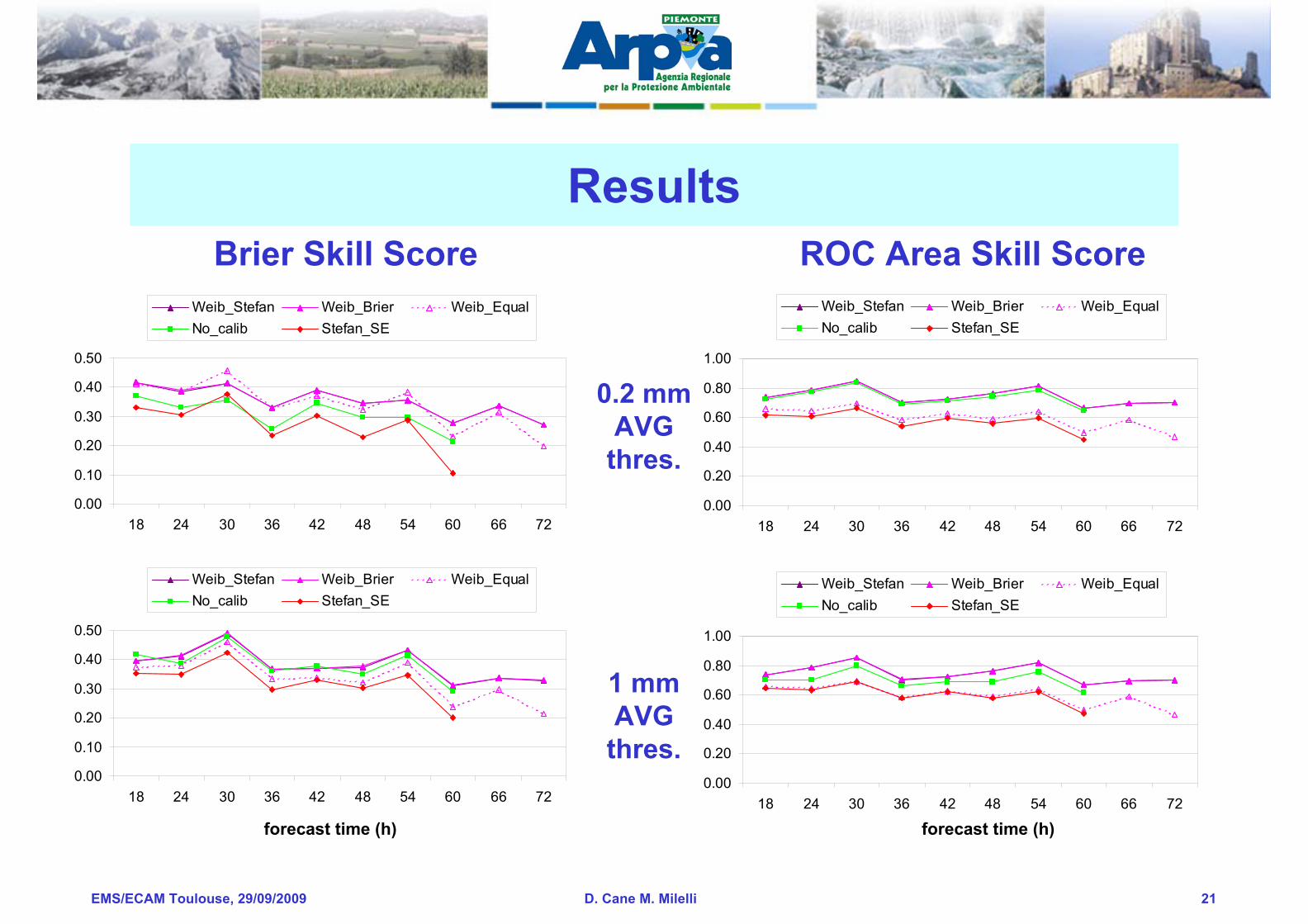
Brier Skill Score ROC Area Skill Score

0.2 mm AVG

thres.

1 mm AVG

thres.

forecast time (h) forecast time (h)


0.00

0.20

0.40

0.60

0.80

1.00

18 24 30 36 42 48 54 60 66 72


0.00

0.10

0.20

0.30

0.40

0.50

18 24 30 36 42 48 54 60 66 72


ResultsBrier Skill Score ROC Area Skill Score

10 mm AVG

thres.


0.00

0.10

0.20

0.30

0.40

0.50

18 24 30 36 42 48 54 60 66 72


0.00

0.20

0.40

0.60

0.80

1.00

18 24 30 36 42 48 54 60 66 72


5 mm AVG

thres.


0.00

0.20

0.40

0.60

0.80

1.00

18 24 30 36 42 48 54 60 66 72


0.00

0.10

0.20

0.30

0.40

0.50

18 24 30 36 42 48 54 60 66 72



5 mm MAX thres.


0.00

0.10

0.20

0.30

0.40

0.50

18 24 30 36 42 48 54 60 66 72


0.00

0.20

0.40

0.60

0.80

1.00

18 24 30 36 42 48 54 60 66 72


1 mm MAX thres.


0.00

0.20

0.40

0.60

0.80

1.00

18 24 30 36 42 48 54 60 66 72


0.00

0.10

0.20

0.30

0.40

0.50

18 24 30 36 42 48 54 60 66 72



20 mm MAX thres.


0.00

0.10

0.20

0.30

0.40

0.50

18 24 30 36 42 48 54 60 66 72


0.00

0.20

0.40

0.60

0.80

1.00

18 24 30 36 42 48 54 60 66 72


10 mm MAX thres.


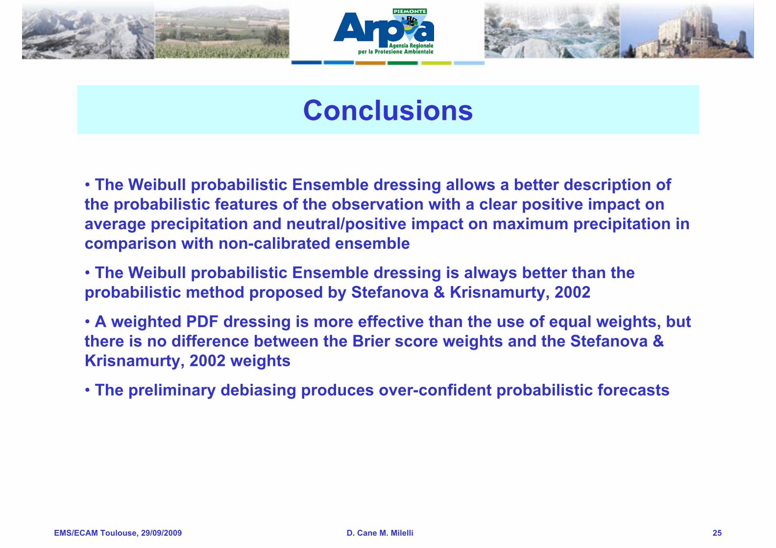
Conclusions

• The Weibull probabilistic Ensemble dressing allows a better description of the probabilistic features of the observation with a clear positive impact on average precipitation and neutral/positive impact on maximum precipitation in comparison with non-calibrated ensemble

• The Weibull probabilistic Ensemble dressing is always better than the probabilistic method proposed by Stefanova & Krisnamurty, 2002

• A weighted PDF dressing is more effective than the use of equal weights, but there is no difference between the Brier score weights and the Stefanova &Krisnamurty, 2002 weights

• The preliminary debiasing produces over-confident probabilistic forecasts


Work in progress

• calculation of the probabilistic PDFs over the whole Italian warning areas system enlarged statistics

• application of the probabilistic precipitation forecasts as the input of our hydrologic chain, evaluation of the discharge calculations uncertainties

• the use of finer spatial resolution (for example: at station locations) will be necessary for this application

• in order to take into account the time variability of the forecasts we are trying to use also the forecast times around the requested leading time


Results

Average precipitation

+ 18h forecast

10 mm threshold

nocalib_debias nocalib_nodebias

SEstef_weib_debias SEstef_weib2_nodebias Brier_weib2_nodebias


Brier Skill Score

0.00

0.05

0.10

0.15

0.20

0.25

0.30

0.35

0.40

0.45

0.50

18 24 30 36 42 48 54 60 66 72

ROC Area Skill Score

0.00

0.10

0.20

0.30

0.40

0.50

0.60

0.70

0.80

0.90

1.00

18 24 30 36 42 48 54 60 66 72

Brier_w eib2_nodebias

UG_w eib2_nodebias

Sestef_w eib2_nodebias

SEstef_w eib_debias

SEstefan_nodebias

SEstefan_debias

Results

Brier Skill Score

0.00

0.05

0.10

0.15

0.20

0.25

0.30

0.35

0.40

0.45

0.50

18 24 30 36 42 48 54 60 66 72


0.00

0.10

0.20

0.30

0.40

0.50

0.60

0.70

0.80

0.90

1.00

18 24 30 36 42 48 54 60 66 72


UG_w eib2_nodebias


SEstef_w eib_debias

SEstefan_nodebias

SEstefan_debias

Average, threshold

1 mm

Average, threshold

10 mm



0.00

0.10

0.20

0.30

0.40

0.50

0.60

0.70

0.80

0.90

1.00

18 24 30 36 42 48 54 60 66 72


UG_w eib2_nodebias


SEstef_w eib_debias

SEstefan_nodebias

SEstefan_debias


0.00

0.10

0.20

0.30

0.40

0.50

0.60

0.70

0.80

0.90

1.00

18 24 30 36 42 48 54 60 66 72


UG_w eib2_nodebias


SEstef_w eib_debias

SEstefan_nodebias

SEstefan_debias

ResultsMaximum, threshold

1 mm

Average, threshold

20 mm

Brier Skill Score

0.00

0.05

0.10

0.15

0.20

0.25

0.30

0.35

0.40

0.45

0.50

18 24 30 36 42 48 54 60 66 72

Brier Skill Score

0.00

0.05

0.10

0.15

0.20

0.25

0.30

0.35

0.40

0.45

0.50

18 24 30 36 42 48 54 60 66 72



0.00

0.10

0.20

0.30

0.40

0.50

0.60

0.70

0.80

0.90

1.00

18 24 30 36 42 48 54 60 66 72


nocalib_debias

nocalib_nodebias


SEstef_w eib_debias


0.00

0.10

0.20

0.30

0.40

0.50

0.60

0.70

0.80

0.90

1.00

18 24 30 36 42 48 54 60 66 72


nocalib_debias

nocalib_nodebias


SEstef_w eib_debias

ResultsAverage, threshold 0.2 mm

Average, threshold

1 mm

Brier Skill Score

0.00

0.05

0.10

0.15

0.20

0.25

0.30

0.35

0.40

0.45

0.50

18 24 30 36 42 48 54 60 66 72

Brier Skill Score

0.00

0.05

0.10

0.15

0.20

0.25

0.30

0.35

0.40

0.45

0.50

18 24 30 36 42 48 54 60 66 72



0.00

0.10

0.20

0.30

0.40

0.50

0.60

0.70

0.80

0.90

1.00

18 24 30 36 42 48 54 60 66 72


nocalib_debias

nocalib_nodebias


SEstef_w eib_debias


0.00

0.10

0.20

0.30

0.40

0.50

0.60

0.70

0.80

0.90

1.00

18 24 30 36 42 48 54 60 66 72


nocalib_debias

nocalib_nodebias


SEstef_w eib_debias

ResultsAverage, threshold

5 mm

Average, threshold

10 mm

Brier Skill Score

0.00

0.05

0.10

0.15

0.20

0.25

0.30

0.35

0.40

0.45

0.50

18 24 30 36 42 48 54 60 66 72

Brier Skill Score

0.00

0.05

0.10

0.15

0.20

0.25

0.30

0.35

0.40

0.45

0.50

18 24 30 36 42 48 54 60 66 72



0.00

0.10

0.20

0.30

0.40

0.50

0.60

0.70

0.80

0.90

1.00

18 24 30 36 42 48 54 60 66 72


nocalib_debias

nocalib_nodebias


SEstef_w eib_debias


0.00

0.10

0.20

0.30

0.40

0.50

0.60

0.70

0.80

0.90

1.00

18 24 30 36 42 48 54 60 66 72


nocalib_debias

nocalib_nodebias


SEstef_w eib_debias


1 mm

Maximum, threshold

5 mm

Brier Skill Score

0.00

0.05

0.10

0.15

0.20

0.25

0.30

0.35

0.40

0.45

0.50

18 24 30 36 42 48 54 60 66 72

Brier Skill Score

0.00

0.05

0.10

0.15

0.20

0.25

0.30

0.35

0.40

0.45

0.50

18 24 30 36 42 48 54 60 66 72



0.00

0.10

0.20

0.30

0.40

0.50

0.60

0.70

0.80

0.90

1.00

18 24 30 36 42 48 54 60 66 72


nocalib_debias

nocalib_nodebias


SEstef_w eib_debias


0.00

0.10

0.20

0.30

0.40

0.50

0.60

0.70

0.80

0.90

1.00

18 24 30 36 42 48 54 60 66 72


nocalib_debias

nocalib_nodebias


SEstef_w eib_debias


10 mm

Maximum, threshold

20 mm

Brier Skill Score

0.00

0.05

0.10

0.15

0.20

0.25

0.30

0.35

0.40

0.45

0.50

18 24 30 36 42 48 54 60 66 72

Brier Skill Score

0.00

0.05

0.10

0.15

0.20

0.25

0.30

0.35

0.40

0.45

0.50

18 24 30 36 42 48 54 60 66 72

New technique for ensemble dressing combining Multimodel SuperEnsemble and precipitation PDF

Documents

Transcript of New technique for ensemble dressing combining Multimodel SuperEnsemble and precipitation PDF