arX

iv:1

103.

1608

v1 [

mat

h-ph

] 8

Mar

201

1

New Symbolic Tools for Differential Geometry, Gravitation, and

Field Theory

I. M. Anderson

Department of Mathematics and Statistics, Utah State University, Logan, Utah 84322, USA

C. G. Torre

Department of Physics, Utah State University, Logan, Utah 84322, USA

March 7, 2011

Abstract

DifferentialGeometry is a Maple software package which symbolically performs fundamental

operations of calculus on manifolds, differential geometry, tensor calculus, Lie algebras, Lie

groups, transformation groups, jet spaces, and the variational calculus. These capabilities,

combined with dramatic recent improvements in symbolic approaches to solving algebraic and

differential equations, have allowed for development of powerful new tools for solving research

problems in gravitation and field theory. The purpose of this paper is to describe some of these

new tools and present some advanced applications involving: Killing vector fields and isometry

groups, Killing tensors and other tensorial invariants, algebraic classification of curvature, and

symmetry reduction of field equations.

1

1 Introduction

DifferentialGeometry is a Maple software package which symbolically performs fundamental

operations of calculus on manifolds, differential geometry, tensor calculus, Lie algebras, Lie

groups, transformation groups, jet spaces, and the variational calculus. These capabilities,

combined with dramatic recent improvements in symbolic approaches to solving algebraic and

differential equations, have allowed for development of powerful new tools for solving research

problems in gravitation and field theory. The purpose of this paper is to describe some of these

new tools and present some advanced applications.

In the next section we show how to symbolically define a chart on a manifold, define tensor

fields on the manifold and perform various routine computations. Such computations feature

in all existing symbolic approaches to the present subject (see, e.g., [1]). We then focus on a

number of applications that take advantage of new mathematical functionalities which, to the

best of our knowledge, have not previously been available in an integrated software package.

In §3 we consider the problem of finding Killing vector fields and determining the structure of

the associated isometry group. As an example we show that the Godel spacetime is a reductive

homogeneous space. Also demonstrated in §3 is how to use DifferentialGeometry to perform

case-splitting analysis, which isolates exceptional values of functions and parameters. This latter

point is illustrated with a family of explicit vacuum metrics in the Kundt class which generically

admit no isometries.

In §4 we consider the various issues associated with algebraic classification of curvature

tensors. We again focus on the ability to perform case splitting when solving equations sym-

bolically to analyze a family of hypersurface homogeneous spacetimes found in [2]. With one

minor correction we confirm the results there and we show that the family of metrics includes

some additional, new Petrov types at exceptional values of parameters appearing in the metric.

Each Petrov type determines a family of adapted null tetrads, a set of principal null directions,

and a factorization of the Weyl spinor, each of which can be obtained symbolically. This we

illustrate with the Godel spacetime.

In §5 we discuss how the vector bundle functionality of DifferentialGeometry allows one to

symbolically implement the formalism of spinor fields. Currently, DifferentialGeometry has a

full implementation of the most important case: the 2-component spinor formalism on a four-

dimensional pseudo-Riemannian manifold. We illustrate this by finding the principal spinors,

which factorize the Weyl spinor, for the Godel spacetime. The algorithms for computing adapted

null tetrads and principal null directions make use of these principal spinors.

In §6 we focus on various tensorial invariants of (pseudo-)Riemannian manifolds such as

homothetic vector fields, Killing tensors and Killing-Yano tensors. In particular, (i) we compute

the homothety group for plane wave spacetimes; (ii) we show how to compute the rank-2 Killing-

Yano tensor and associated Killing tensor for Kerr spacetime; and (iii) we show that the Godel

spacetime has no non-trivial Killing tensors of rank-2 and rank-3.

Finally, in §7 we symbolically analyze the process of reduction of field equations by a pre-

scribed group of symmetries in the context of gravitational plane waves. In particular we show

how DifferentialGeometry can be used to find the most general group-invariant metric and to

find the residual symmetry group admitted by the reduced field equations.

2

In DifferentialGeometry all tensor fields, spinor fields, connections, and so forth are built

and displayed using index-free notation as is standard in the mathematical literature. Differ-

entialGeometry runs as a package in Maple (see, e.g., [3]) and the syntax of all commands and

output which we describe reflects this.1 We have taken a few liberties with the output of some

of the commands to make it more readable in this venue. See the Appendix for a complete list

of all the available commands. DifferentialGeometry first appeared in Maple 11; much of the

capabilities described here appear in Maple 14 and Maple 15. Full documentation and tutorials

can also be found in these releases. We note that the underlying code for all DifferentialGeome-

try commands can be explicitly displayed so that, if desired, one can have complete control over

the details of all computations.

It is a pleasure to thank Edgardo Cheb-Terrab, first for proposing the development of general

relativity tools within the framework ofDifferentialGeometry, and second, for his time and efforts

to integrate this work into the Maple distributed library of packages. Support from the National

Science Foundation (DMS-0713830) and Maplesoft is gratefully acknowledged.

2 Manifolds, tensor fields, frames

When analyzing a (pseudo-)Riemannian manifold using DifferentialGeometry the first order of

business is to define a chart on the manifold where computations will take place and to specify a

metric (or some other element of structure). Defining the chart in DifferentialGeometry simply

amounts to specifying the names of coordinates which will be used and specifying a name for the

chart. (Other charts and coordinates can be defined subsequently as desired.) The command

for defining a chart is DGsetup. Here we define a chart named M with coordinates (t, r, θ, φ).

> DGsetup([t, r, theta, phi], M):

This specifies the dimension of the manifold, it protects the coordinate labels and it defines

coordinate basis vector fields and forms.

All tensor operations are supported; there are commands for scalar multiplication, tensor

product, tensor addition, contraction of indices, symmetrization of indices, and so forth. The

command evalDG can be used to allow a streamlined syntax for some of these operations. In

particular, within evalDG one can build tensor fields using the asterisk for scalar multiplication,

using ± for tensor addition/subtraction, using &t for tensor product, using &w for wedge product,

and using &s for symmetric tensor product.

One can now specify fields on the manifold M . For example, one often wants to begin

by specifying a metric in the coordinate basis. We do this as follows using the the Reissner-

Nordstrom metric with mass M and charge Q as an example. For convenience, we first define

some standard notation:

> f := 1 - 2*M/r + Q^2/r^2:

> dOmega := evalDG(dtheta &t dtheta + sin(theta)^2*dphi &t dphi):

1Note, in particular, that a command terminated with a colon will suppress displaying the results of the command,

while a command terminated with a semi-colon will display the results of the command.

3

The metric is now defined by

> g := evalDG(-f*dt &t dt + 1/f*dr &t dr + r^2*dOmega);

g := (−1 +2M

r− Q2

r2)dt dt+

r2

r2 − 2Mr +Q2dr dr + r2(dθ dθ + sin(θ)2dφ dφ)

Note that the tensor product is implicit in the Maple output. Next we define the Reissner-

Nordstrom electromagnetic field F as a spacetime 2-form:

> F := evalDG(sqrt(2)*Q/r^2*dt &w dr);

F :=

√2Q

r2dt ∧ dr

A number of frequently used tensor fields are pre-defined for convenience. For example,

energy momentum tensors can be computed once the type of field and relevant geometric data

are supplied. Here we compute the energy-momentum tensor of the Reissner-Nordstrom elec-

tromagnetic field:

> T := EnergyMomentumTensor(‘‘Electromagnetic’’, g, F);

T :=Q2

r2(r2 − 2Mr +Q2)DtDt −

Q2(r2 − 2Mr +Q2)

r6DrDr +

Q2

r6DθDθ +

Q2

r6 sin(θ)2DφDφ

Note that T has been defined as a tensor of type(

20

)

; the quantities (Dt, DrDθ, Dφ) are the

coordinate basis vector fields. Here we verify that g and F determine a solution to the Einstein-

Maxwell equations. First we check the Einstein equations:

> G:= EinsteinTensor(g):

> evalDG(G - T);

0DtDt

Next we check the source-free Maxwell equations by verifying ∇ · F = 0 and dF = 0. This can

be done using the CovariantDerivative command and the various tensor operations. Again,

for convenience, these computations are pre-defined. ∇ · F and dF are given by, respectively,

> MatterFieldEquations(‘‘Electromagnetic’’, g, F);

0Dt, 0 dt ∧ dr ∧ dθ

It is also possible to define fields relative to a given anholonomic frame. This is often the

most effective setting in which to perform complex computations. We illustrate this with the

Reissner-Nordstrom spacetime.

4

We begin by defining an orthonormal tetrad OT as a list of vector fields.

> OT := evalDG([1/sqrt(f) * D t, sqrt(f) * D r, D theta/r, D phi/(r*sin(theta))]);

OT := [r

√

r2 − 2Mr +Q2Dt,

√

r2 − 2Mr +Q2

rDr,

1

rDθ,

1

r sin(θ)Dφ]

We can verify this is in fact an orthonormal tetrad by computing the 10 scalar products between

these vector fields using the metric g. A shortcut is the TensorInnerProduct command which

will take any two (lists of) tensors of the same type and contract all indices with a specified

metric. Using the list OT the output is the matrix of scalar products:

> TensorInnerProduct(g, OT, OT);

−1 0 0 0

0 1 0 0

0 0 1 0

0 0 0 1

When working in an orthonormal frame the structure equations of the frame, i.e., the commu-

tation relations of the frame vector fields, determine all the geometric properties of the space-

time. These structure equations are computed and stored for future use using the commands

FrameData and DGsetup, respectively:

> FD := FrameData(OT, O);

FD :=[

[E1, E2] = − Mr −Q2

r2√

r2 − 2Mr +Q2E1, [E2, E3] = −

√

r2 − 2Mr +Q2

r2E3,

[E2, E4] = −√

r2 − 2Mr +Q2

r2E4, [E3, E4] = − cos(θ)

r sin(θ)E4

]

> DGsetup(FD):

The (default) labeling for the basis vectors is (E1, E2, E3, E4), the (default) labeling for the

dual basis is (Θ1, . . . ,Θ4). The variable FD contains all their commutators as well as the name

(O) chosen for the anholonomic frame.

One can now perform all computations in the given orthonormal frame. Here we define the

metric in this orthonormal frame:

> eta := evalDG(- Theta1 &t Theta1 + Theta2 &t Theta2

+ Theta3 &t Theta3 + Theta4 &t Theta4);

η := −Θ1Θ1+ Θ2Θ2 + Θ3Θ3 + Θ4Θ4

The Ricci tensor takes the form:

5

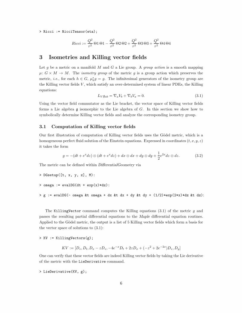
> Ricci := RicciTensor(eta);

Ricci :=Q2

r2Θ1Θ1− Q2

r2Θ2Θ2+

Q2

r2Θ3Θ3+

Q2

r2Θ4Θ4

3 Isometries and Killing vector fields

Let g be a metric on a manifold M and G a Lie group. A group action is a smooth mapping

µ : G × M → M . The isometry group of the metric g is a group action which preserves the

metric, i.e., for each h ∈ G, µ∗

hg = g. The infinitesimal generators of the isometry group are

the Killing vector fields V , which satisfy an over-determined system of linear PDEs, the Killing

equations:

LV gab = ∇aVb +∇bVa = 0. (3.1)

Using the vector field commutator as the Lie bracket, the vector space of Killing vector fields

forms a Lie algebra g isomorphic to the Lie algebra of G. In this section we show how to

symbolically determine Killing vector fields and analyze the corresponding isometry group.

3.1 Computation of Killing vector fields

Our first illustration of computation of Killing vector fields uses the Godel metric, which is a

homogeneous perfect fluid solution of the Einstein equations. Expressed in coordinates (t, x, y, z)

it takes the form

g = −(dt+ exdz)⊗ (dt+ exdz) + dx⊗ dx+ dy ⊗ dy +1

2e2xdz ⊗ dz. (3.2)

The metric can be defined within DifferentialGeometry via

> DGsetup([t, x, y, z], M):

> omega := evalDG(dt + exp(x)*dz):

> g := evalDG(- omega &t omega + dx &t dx + dy &t dy + (1/2)*exp(2*x)*dz &t dz):

The KillingVector command computes the Killing equations (3.1) of the metric g and

passes the resulting partial differential equations to the Maple differential equation routines.

Applied to the Godel metric, the output is a list of 5 Killing vector fields which form a basis for

the vector space of solutions to (3.1):

> KV := KillingVectors(g);

KV := [Dz, Dt, Dx − zDz,−4e−xDt + 2zDx + (−z2 + 2e−2x)Dz, Dy]

One can verify that these vector fields are indeed Killing vector fields by taking the Lie derivative

of the metric with the LieDerivative command.

> LieDerivative(KV, g);

6

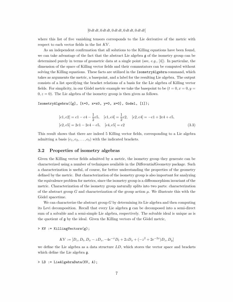
[0 dt dt, 0 dt dt, 0 dt dt, 0 dt dt, 0 dt dt]

where this list of five vanishing tensors corresponds to the Lie derivative of the metric with

respect to each vector fields in the list KV .

As an independent confirmation that all solutions to the Killing equations have been found,

we can take advantage of the fact that the abstract Lie algebra g of the isometry group can be

determined purely in terms of geometric data at a single point (see, e.g., [4]). In particular, the

dimension of the space of Killing vector fields and their commutators can be computed without

solving the Killing equations. These facts are utilized in the IsometryAlgebra command, which

takes as arguments the metric, a basepoint, and a label for the resulting Lie algebra. The output

consists of a list specifying the bracket relations of a basis for the Lie algebra of Killing vector

fields. For simplicity, in our Godel metric example we take the basepoint to be (t = 0, x = 0, y =

0, z = 0). The Lie algebra of the isometry group is then given as follows.

IsometryAlgebra([g], [t=0, x=x0, y=0, z=0], Godel, [1]);

[e1, e2] = e1− e4− 1

2e5, [e1, e4] =

1

2e2, [e2, e4] = −e1 + 2e4 + e5,

[e2, e5] = 2e1− 2e4− e5, [e4, e5] = e2 (3.3)

This result shows that there are indeed 5 Killing vector fields, corresponding to a Lie algebra

admitting a basis (e1, e2, . . . , e5) with the indicated brackets.

3.2 Properties of isometry algebras

Given the Killing vector fields admitted by a metric, the isometry group they generate can be

characterized using a number of techniques available in the DifferentialGeometry package. Such

a characterization is useful, of course, for better understanding the properties of the geometry

defined by the metric. But characterization of the isometry group is also important for analyzing

the equivalence problem for metrics, since the isometry group is a diffeomorphism invariant of the

metric. Characterization of the isometry group naturally splits into two parts: characterization

of the abstract group G and characterization of the group action µ. We illustrate this with the

Godel spacetime.

We can characterize the abstract group G by determining its Lie algebra and then computing

its Levi decomposition. Recall that every Lie algebra g can be decomposed into a semi-direct

sum of a solvable and a semi-simple Lie algebra, respectively. The solvable ideal is unique as is

the quotient of g by the ideal. Given the Killing vectors of the Godel metric,

> KV := KillingVectors(g);

KV := [Dz, Dt, Dx − zDz,−4e−xDt + 2zDx + (−z2 + 2e−2x)Dz, Dy]

we define the Lie algebra as a data structure LD, which stores the vector space and brackets

which define the Lie algebra g.

> LD := LieAlgebraData(KV, A);

7

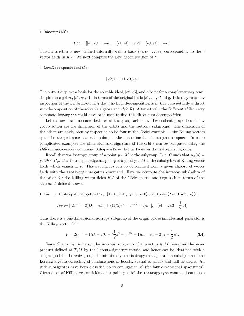
> DGsetup(LD):

LD := [[e1, e3] = −e1, [e1, e4] = 2 e3, [e3, e4] = −e4]

The Lie algebra is now defined internally with a basis (e1, e2, . . . , e5) corresponding to the 5

vector fields in KV . We next compute the Levi decomposition of g

> LeviDecomposition(A);

[[e2, e5], [e1, e3, e4]]

The output displays a basis for the solvable ideal, [e2, e5], and a basis for a complementary semi-

simple sub-algebra, [e1, e3, e4], in terms of the original basis [e1, . . . , e5] of g. It is easy to see by

inspection of the Lie brackets in g that the Levi decomposition is in this case actually a direct

sum decomposition of the solvable algebra and sl(2, R). Alternatively, the DifferentialGeometry

command Decompose could have been used to find this direct sum decomposition.

Let us now examine some features of the group action µ. Two salient properties of any

group action are the dimension of the orbits and the isotropy subgroups. The dimension of

the orbits are easily seen by inspection to be four in the Godel example — the Killing vectors

span the tangent space at each point, so the spacetime is a homogeneous space. In more

complicated examples the dimension and signature of the orbits can be computed using the

DifferentialGeometry command SubspaceType. Let us focus on the isotropy subgroups.

Recall that the isotropy group of a point p ∈ M is the subgroup Gp ⊂ G such that µh(p) =

p, ∀h ∈ Gp. The isotropy subalgebra gp ⊂ g of a point p ∈ M is the subalgebra of Killing vector

fields which vanish at p. This subalgebra can be determined from a given algebra of vector

fields with the IsotropySubalgebra command. Here we compute the isotropy subalgebra of

the origin for the Killing vector fields KV of the Godel metric and express it in terms of the

algebra A defined above:

> Iso := IsotropySubalgebra(KV, [t=0, x=0, y=0, z=0], output=["Vector", A]);

Iso := [(2e−x − 2)Dt − zDx + ((1/2)z2 − e−2x + 1)Dz], [e1− 2 e2− 1

2e4]

Thus there is a one dimensional isotropy subgroup of the origin whose infinitesimal generator is

the Killing vector field

V = 2(e−x − 1)∂t − z∂x + (1

2z2 − e−2x + 1)∂z = e1− 2 e2− 1

2e4. (3.4)

Since G acts by isometry, the isotropy subgroup of a point p ∈ M preserves the inner

product defined at TpM by the Lorentz-signature metric, and hence can be identified with a

subgroup of the Lorentz group. Infinitesimally, the isotropy subalgebra is a subalgebra of the

Lorentz algebra consisting of combinations of boosts, spatial rotations and null rotations. All

such subalgebras have been classified up to conjugation [5] (for four dimensional spacetimes).

Given a set of Killing vector fields and a point p ∈ M the IsotropyType command computes

8

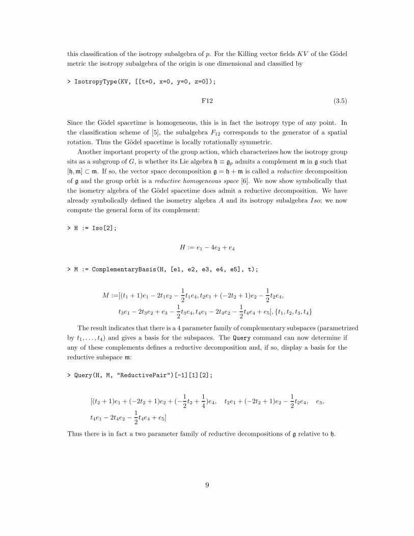
this classification of the isotropy subalgebra of p. For the Killing vector fields KV of the Godel

metric the isotropy subalgebra of the origin is one dimensional and classified by

> IsotropyType(KV, [[t=0, x=0, y=0, z=0]);

F12 (3.5)

Since the Godel spacetime is homogeneous, this is in fact the isotropy type of any point. In

the classification scheme of [5], the subalgebra F12 corresponds to the generator of a spatial

rotation. Thus the Godel spacetime is locally rotationally symmetric.

Another important property of the group action, which characterizes how the isotropy group

sits as a subgroup of G, is whether its Lie algebra h ≡ gp admits a complement m in g such that

[h,m] ⊂ m. If so, the vector space decomposition g = h+m is called a reductive decomposition

of g and the group orbit is a reductive homogeneous space [6]. We now show symbolically that

the isometry algebra of the Godel spacetime does admit a reductive decomposition. We have

already symbolically defined the isometry algebra A and its isotropy subalgebra Iso; we now

compute the general form of its complement:

> H := Iso[2];

H := e1 − 4e2 + e4

> M := ComplementaryBasis(H, [e1, e2, e3, e4, e5], t);

M :=[(t1 + 1)e1 − 2t1e2 −1

2t1e4, t2e1 + (−2t2 + 1)e2 −

1

2t2e4,

t3e1 − 2t3e2 + e3 −1

2t3e4, t4e1 − 2t4e2 −

1

2t4e4 + e5], {t1, t2, t3, t4}

The result indicates that there is a 4 parameter family of complementary subspaces (parametrized

by t1, . . . , t4) and gives a basis for the subspaces. The Query command can now determine if

any of these complements defines a reductive decomposition and, if so, display a basis for the

reductive subspace m:

> Query(H, M, "ReductivePair")[-1][1][2];

[(t2 + 1)e1 + (−2t2 + 1)e2 + (−1

2t2 +

1

4)e4, t2e1 + (−2t2 + 1)e2 −

1

2t2e4, e3,

t4e1 − 2t4e2 −1

2t4e4 + e5]

Thus there is in fact a two parameter family of reductive decompositions of g relative to h.

9

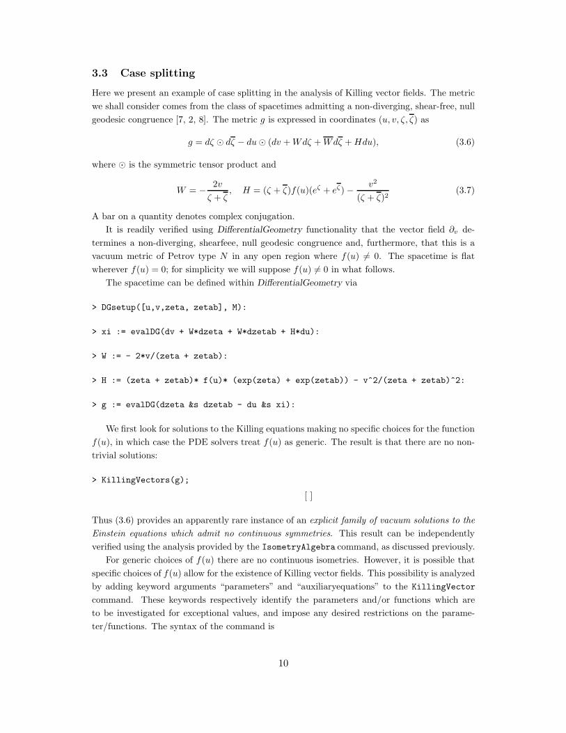
3.3 Case splitting

Here we present an example of case splitting in the analysis of Killing vector fields. The metric

we shall consider comes from the class of spacetimes admitting a non-diverging, shear-free, null

geodesic congruence [7, 2, 8]. The metric g is expressed in coordinates (u, v, ζ, ζ) as

g = dζ ⊙ dζ − du⊙ (dv +Wdζ +Wdζ +Hdu), (3.6)

where ⊙ is the symmetric tensor product and

W = − 2v

ζ + ζ, H = (ζ + ζ)f(u)(eζ + eζ)− v2

(ζ + ζ)2(3.7)

A bar on a quantity denotes complex conjugation.

It is readily verified using DifferentialGeometry functionality that the vector field ∂v de-

termines a non-diverging, shearfeee, null geodesic congruence and, furthermore, that this is a

vacuum metric of Petrov type N in any open region where f(u) 6= 0. The spacetime is flat

wherever f(u) = 0; for simplicity we will suppose f(u) 6= 0 in what follows.

The spacetime can be defined within DifferentialGeometry via

> DGsetup([u,v,zeta, zetab], M):

> xi := evalDG(dv + W*dzeta + W*dzetab + H*du):

> W := - 2*v/(zeta + zetab):

> H := (zeta + zetab)* f(u)* (exp(zeta) + exp(zetab)) - v^2/(zeta + zetab)^2:

> g := evalDG(dzeta &s dzetab - du &s xi):

We first look for solutions to the Killing equations making no specific choices for the function

f(u), in which case the PDE solvers treat f(u) as generic. The result is that there are no non-

trivial solutions:

> KillingVectors(g);

[ ]

Thus (3.6) provides an apparently rare instance of an explicit family of vacuum solutions to the

Einstein equations which admit no continuous symmetries. This result can be independently

verified using the analysis provided by the IsometryAlgebra command, as discussed previously.

For generic choices of f(u) there are no continuous isometries. However, it is possible that

specific choices of f(u) allow for the existence of Killing vector fields. This possibility is analyzed

by adding keyword arguments “parameters” and “auxiliaryequations” to the KillingVector

command. These keywords respectively identify the parameters and/or functions which are

to be investigated for exceptional values, and impose any desired restrictions on the parame-

ter/functions. The syntax of the command is

10

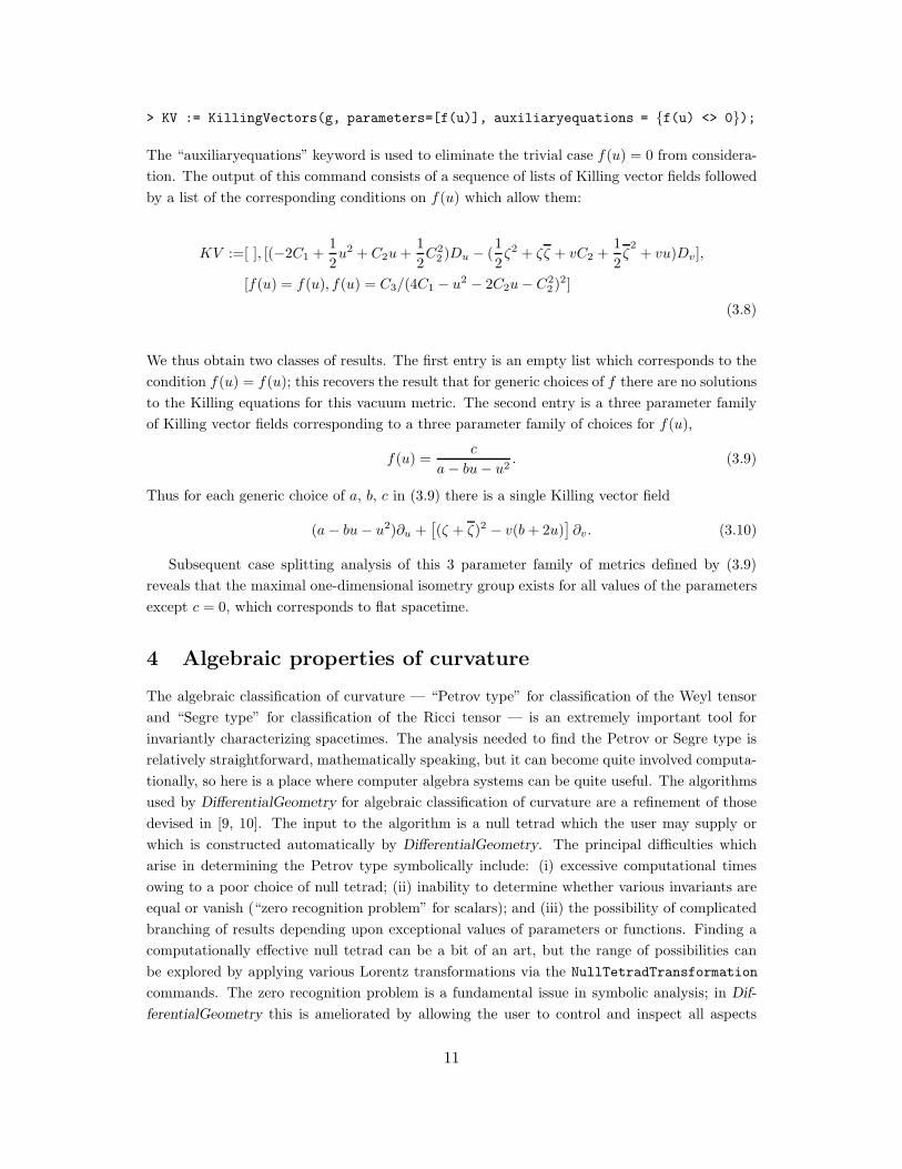
> KV := KillingVectors(g, parameters=[f(u)], auxiliaryequations = {f(u) <> 0});

The “auxiliaryequations” keyword is used to eliminate the trivial case f(u) = 0 from considera-

tion. The output of this command consists of a sequence of lists of Killing vector fields followed

by a list of the corresponding conditions on f(u) which allow them:

KV :=[ ], [(−2C1 +1

2u2 + C2u+

1

2C2

2 )Du − (1

2ζ2 + ζζ + vC2 +

1

2ζ2+ vu)Dv],

[f(u) = f(u), f(u) = C3/(4C1 − u2 − 2C2u− C22 )

2]

(3.8)

We thus obtain two classes of results. The first entry is an empty list which corresponds to the

condition f(u) = f(u); this recovers the result that for generic choices of f there are no solutions

to the Killing equations for this vacuum metric. The second entry is a three parameter family

of Killing vector fields corresponding to a three parameter family of choices for f(u),

f(u) =c

a− bu− u2. (3.9)

Thus for each generic choice of a, b, c in (3.9) there is a single Killing vector field

(a− bu− u2)∂u +[

(ζ + ζ)2 − v(b+ 2u)]

∂v. (3.10)

Subsequent case splitting analysis of this 3 parameter family of metrics defined by (3.9)

reveals that the maximal one-dimensional isometry group exists for all values of the parameters

except c = 0, which corresponds to flat spacetime.

4 Algebraic properties of curvature

The algebraic classification of curvature — “Petrov type” for classification of the Weyl tensor

and “Segre type” for classification of the Ricci tensor — is an extremely important tool for

invariantly characterizing spacetimes. The analysis needed to find the Petrov or Segre type is

relatively straightforward, mathematically speaking, but it can become quite involved computa-

tionally, so here is a place where computer algebra systems can be quite useful. The algorithms

used by DifferentialGeometry for algebraic classification of curvature are a refinement of those

devised in [9, 10]. The input to the algorithm is a null tetrad which the user may supply or

which is constructed automatically by DifferentialGeometry. The principal difficulties which

arise in determining the Petrov type symbolically include: (i) excessive computational times

owing to a poor choice of null tetrad; (ii) inability to determine whether various invariants are

equal or vanish (“zero recognition problem” for scalars); and (iii) the possibility of complicated

branching of results depending upon exceptional values of parameters or functions. Finding a

computationally effective null tetrad can be a bit of an art, but the range of possibilities can

be explored by applying various Lorentz transformations via the NullTetradTransformation

commands. The zero recognition problem is a fundamental issue in symbolic analysis; in Dif-

ferentialGeometry this is ameliorated by allowing the user to control and inspect all aspects

11

of the classification process. In particular, the infolevel command allows the user to inspect

each step of the classification algorithm, the Preferences command allows the user to create

custom-made simplification rules, and the output option allows the user to examine the various

algebraic and differential equations which arise in determining the algebraic classification. Pos-

sible branching of the classification is handled using customizable case-splitting analysis options.

We illustrate some of this with the following computations of Petrov type.

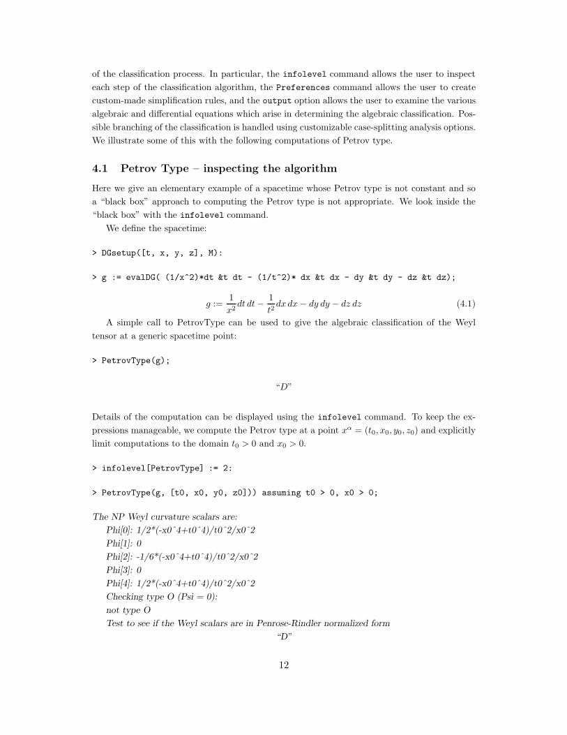
4.1 Petrov Type – inspecting the algorithm

Here we give an elementary example of a spacetime whose Petrov type is not constant and so

a “black box” approach to computing the Petrov type is not appropriate. We look inside the

“black box” with the infolevel command.

We define the spacetime:

> DGsetup([t, x, y, z], M):

> g := evalDG( (1/x^2)*dt &t dt - (1/t^2)* dx &t dx - dy &t dy - dz &t dz);

g :=1

x2dt dt− 1

t2dx dx− dy dy − dz dz (4.1)

A simple call to PetrovType can be used to give the algebraic classification of the Weyl

tensor at a generic spacetime point:

> PetrovType(g);

“D”

Details of the computation can be displayed using the infolevel command. To keep the ex-

pressions manageable, we compute the Petrov type at a point xα = (t0, x0, y0, z0) and explicitly

limit computations to the domain t0 > 0 and x0 > 0.

> infolevel[PetrovType] := 2:

> PetrovType(g, [t0, x0, y0, z0])) assuming t0 > 0, x0 > 0;

The NP Weyl curvature scalars are:

Phi[0]: 1/2*(-x0ˆ4+t0ˆ4)/t0ˆ2/x0ˆ2

Phi[1]: 0

Phi[2]: -1/6*(-x0ˆ4+t0ˆ4)/t0ˆ2/x0ˆ2

Phi[3]: 0

Phi[4]: 1/2*(-x0ˆ4+t0ˆ4)/t0ˆ2/x0ˆ2

Checking type O (Psi = 0):

not type O

Test to see if the Weyl scalars are in Penrose-Rindler normalized form

“D”

12

As can be seen from this output, the algorithm first computes the Newman-Penrose Weyl cur-

vature scalars, which are to be used to construct various scalar curvature invariants determining

the Petrov type. The curvature scalars are first tested to see if they all vanish, in which case

the Petrov type is O. It is clear from the scalar invariants displayed above that they are non-

vanishing everywhere except on the null hypersurfaces x = ±t. Away from these hypersurfaces,

the curvature scalars are in a normal form for type D spacetimes and the algorithm terminates.

By computing the Petrov type at an exceptional point, say x = t = a, we confirm that the

spacetime is of type O at such points:

> PetrovType(g, [t=a, x=a, y=y0, z=z0]);

“O”

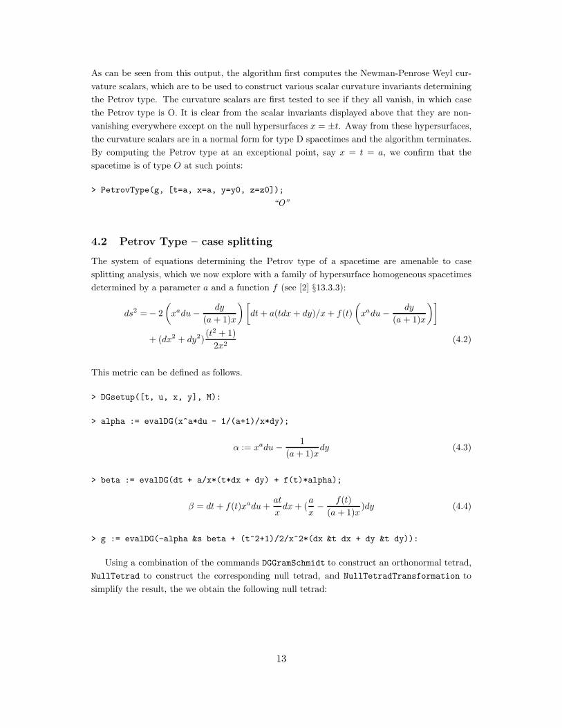
4.2 Petrov Type – case splitting

The system of equations determining the Petrov type of a spacetime are amenable to case

splitting analysis, which we now explore with a family of hypersurface homogeneous spacetimes

determined by a parameter a and a function f (see [2] §13.3.3):

ds2 =− 2

(

xadu− dy

(a+ 1)x

)[

dt+ a(tdx+ dy)/x+ f(t)

(

xadu− dy

(a+ 1)x

)]

+ (dx2 + dy2)(t2 + 1)

2x2(4.2)

This metric can be defined as follows.

> DGsetup([t, u, x, y], M):

> alpha := evalDG(x^a*du - 1/(a+1)/x*dy);

α := xadu − 1

(a+ 1)xdy (4.3)

> beta := evalDG(dt + a/x*(t*dx + dy) + f(t)*alpha);

β = dt+ f(t)xadu+at

xdx+ (

a

x− f(t)

(a+ 1)x)dy (4.4)

> g := evalDG(-alpha &s beta + (t^2+1)/2/x^2*(dx &t dx + dy &t dy)):

Using a combination of the commands DGGramSchmidt to construct an orthonormal tetrad,

NullTetrad to construct the corresponding null tetrad, and NullTetradTransformation to

simplify the result, the we obtain the following null tetrad:

13

NT :=[Dt,−f(t)Dt + x−aDu,

− a(I + t)√t2 + 1

Dt +Ix−a

√t2 + 1(a+ 1)

Du +x√

t2 + 1Dx +

Ix√t2 + 1

Dy,

a(I − t)√t2 + 1

Dt −Ix−a

√t2 + 1(a+ 1)

Du +x√

t2 + 1Dx − Ix√

t2 + 1Dy]

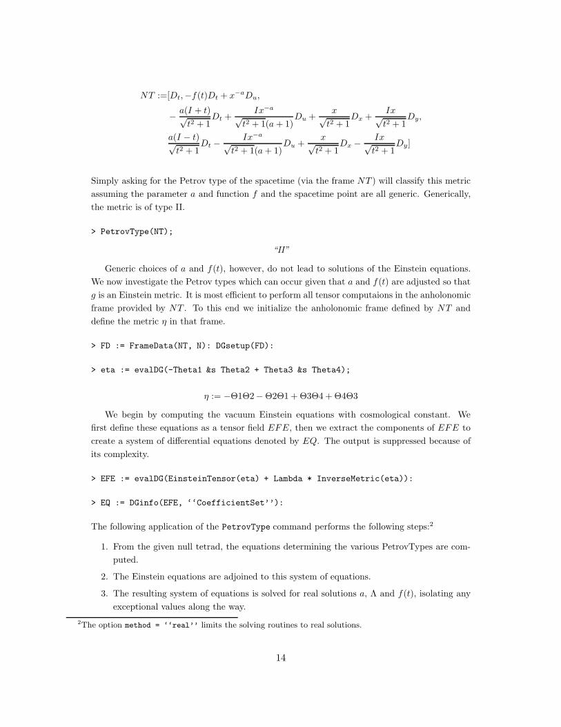
Simply asking for the Petrov type of the spacetime (via the frame NT ) will classify this metric

assuming the parameter a and function f and the spacetime point are all generic. Generically,

the metric is of type II.

> PetrovType(NT);

“II”

Generic choices of a and f(t), however, do not lead to solutions of the Einstein equations.

We now investigate the Petrov types which can occur given that a and f(t) are adjusted so that

g is an Einstein metric. It is most efficient to perform all tensor computaions in the anholonomic

frame provided by NT . To this end we initialize the anholonomic frame defined by NT and

define the metric η in that frame.

> FD := FrameData(NT, N): DGsetup(FD):

> eta := evalDG(-Theta1 &s Theta2 + Theta3 &s Theta4);

η := −Θ1Θ2−Θ2Θ1 + Θ3Θ4 + Θ4Θ3

We begin by computing the vacuum Einstein equations with cosmological constant. We

first define these equations as a tensor field EFE, then we extract the components of EFE to

create a system of differential equations denoted by EQ. The output is suppressed because of

its complexity.

> EFE := evalDG(EinsteinTensor(eta) + Lambda * InverseMetric(eta)):

> EQ := DGinfo(EFE, ‘‘CoefficientSet’’):

The following application of the PetrovType command performs the following steps:2

1. From the given null tetrad, the equations determining the various PetrovTypes are com-

puted.

2. The Einstein equations are adjoined to this system of equations.

3. The resulting system of equations is solved for real solutions a, Λ and f(t), isolating any

exceptional values along the way.

2The option method = ‘‘real’’ limits the solving routines to real solutions.

14

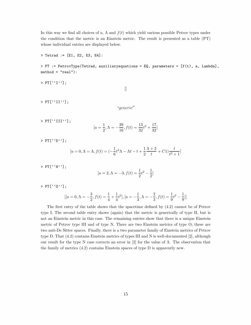
In this way we find all choices of a, Λ and f(t) which yield various possible Petrov types under

the condition that the metric is an Einstein metric. The result is presented as a table (PT)

whose individual entries are displayed below.

> Tetrad := [E1, E2, E3, E4]:

> PT := PetrovType(Tetrad, auxiliaryequations = EQ, parameters = [f(t), a, Lambda],

method = "real"):

> PT[‘‘I’’];

[]

> PT[‘‘II’’];

“generic′′

> PT[‘‘III’’];

[a =1

2,Λ = −39

16, f(t) =

13

32t2 +

17

32]

> PT[‘‘D’’];

[a = 0,Λ = Λ, f(t) = (−1

6t3Λ− Λt− t+

1

2

Λ + 2

t+ C1)

t

t2 + 1]

> PT[‘‘N’’];

[a = 2,Λ = −3, f(t) =1

2t2 − 1

2]

> PT[‘‘O’’];

[[a = 0,Λ = −3

2, f(t) =

1

4+

1

4t2], [a = −1

3,Λ = −2

3, f(t) =

1

9t2 − 1

9]]

The first entry of the table shows that the spacetime defined by (4.2) cannot be of Petrov

type I. The second table entry shows (again) that the metric is generically of type II, but is

not an Einstein metric in this case. The remaining entries show that there is a unique Einstein

metric of Petrov type III and of type N. There are two Einstein metrics of type O; these are

two anti-De Sitter spaces. Finally, there is a two parameter family of Einstein metrics of Petrov

type D. That (4.2) contains Einstein metrics of types III and N is well-documented [2], although

our result for the type N case corrects an error in [2] for the value of Λ. The observation that

the family of metrics (4.2) contains Einstein spaces of type D is apparently new.

15

4.3 Adapted tetrads and principal null directions

Each Petrov type admits a family of adapted null tetrads which put the Newman-Penrose Weyl

scalars into a normal form [11]. Such tetrads can be viewed as optimized for virtually all

computations in open regions of spacetime where the Petrov type is constant. Closely related

to these tetrads are the principal null directions, which give important geometrical information

about a spacetime. Here we show DifferentialGeometry can be used to find the adapted null

tetrads and principal null directions for the Godel spacetime. Computation of adapted null

tetrads and principal null directions both rely upon factorizing the Weyl spinor. The spinor

capabilities of DifferentialGeometry are detailed in the next section.

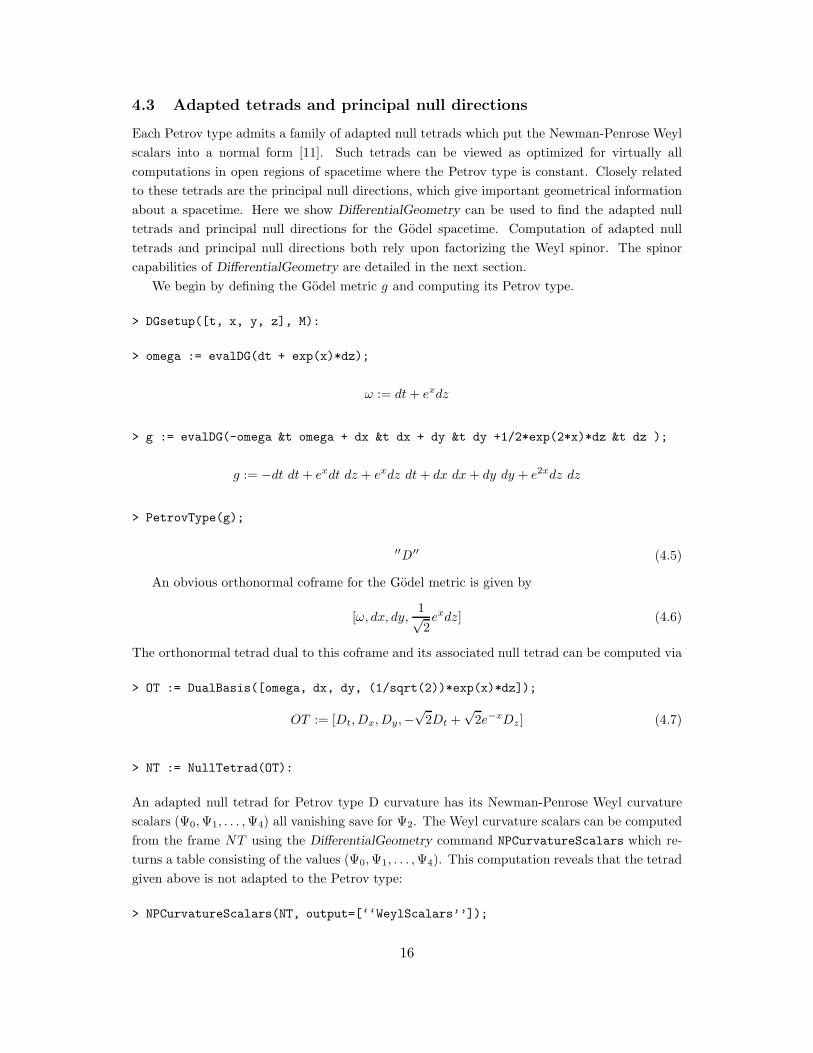
We begin by defining the Godel metric g and computing its Petrov type.

> DGsetup([t, x, y, z], M):

> omega := evalDG(dt + exp(x)*dz);

ω := dt+ exdz

> g := evalDG(-omega &t omega + dx &t dx + dy &t dy +1/2*exp(2*x)*dz &t dz );

g := −dt dt+ exdt dz + exdz dt+ dx dx+ dy dy + e2xdz dz

> PetrovType(g);

′′D ′′ (4.5)

An obvious orthonormal coframe for the Godel metric is given by

[ω, dx, dy,1√2exdz] (4.6)

The orthonormal tetrad dual to this coframe and its associated null tetrad can be computed via

> OT := DualBasis([omega, dx, dy, (1/sqrt(2))*exp(x)*dz]);

OT := [Dt, Dx, Dy,−√2Dt +

√2e−xDz] (4.7)

> NT := NullTetrad(OT):

An adapted null tetrad for Petrov type D curvature has its Newman-Penrose Weyl curvature

scalars (Ψ0,Ψ1, . . . ,Ψ4) all vanishing save for Ψ2. The Weyl curvature scalars can be computed

from the frame NT using the DifferentialGeometry command NPCurvatureScalars which re-

turns a table consisting of the values (Ψ0,Ψ1, . . . ,Ψ4). This computation reveals that the tetrad

given above is not adapted to the Petrov type:

> NPCurvatureScalars(NT, output=[‘‘WeylScalars’’]);

16

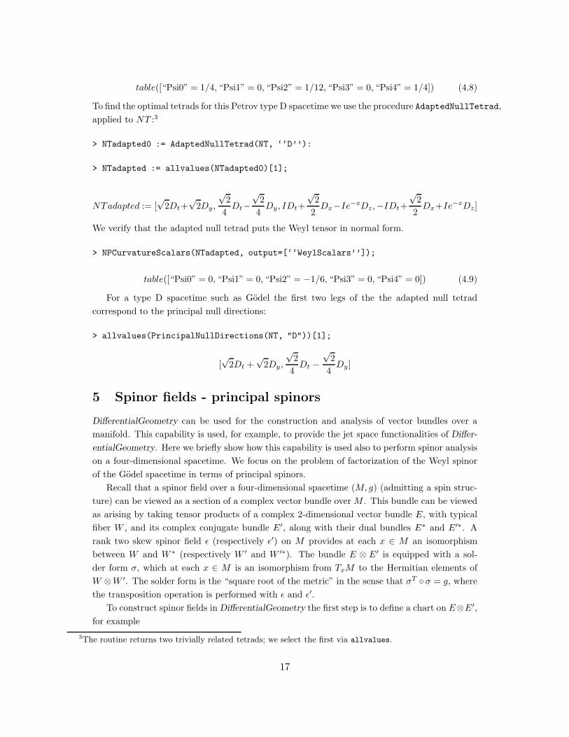
table([“Psi0” = 1/4, “Psi1” = 0, “Psi2” = 1/12, “Psi3” = 0, “Psi4” = 1/4]) (4.8)

To find the optimal tetrads for this Petrov type D spacetime we use the procedure AdaptedNullTetrad,

applied to NT :3

> NTadapted0 := AdaptedNullTetrad(NT, ‘‘D’’):

> NTadapted := allvalues(NTadapted0)[1];

NTadapted := [√2Dt+

√2Dy,

√2

4Dt−

√2

4Dy, IDt+

√2

2Dx−Ie−xDz,−IDt+

√2

2Dx+Ie−xDz]

We verify that the adapted null tetrad puts the Weyl tensor in normal form.

> NPCurvatureScalars(NTadapted, output=[‘‘WeylScalars’’]);

table([“Psi0” = 0, “Psi1” = 0, “Psi2” = −1/6, “Psi3” = 0, “Psi4” = 0]) (4.9)

For a type D spacetime such as Godel the first two legs of the the adapted null tetrad

correspond to the principal null directions:

> allvalues(PrincipalNullDirections(NT, "D"))[1];

[√2Dt +

√2Dy,

√2

4Dt −

√2

4Dy]

5 Spinor fields - principal spinors

DifferentialGeometry can be used for the construction and analysis of vector bundles over a

manifold. This capability is used, for example, to provide the jet space functionalities of Differ-

entialGeometry. Here we briefly show how this capability is used also to perform spinor analysis

on a four-dimensional spacetime. We focus on the problem of factorization of the Weyl spinor

of the Godel spacetime in terms of principal spinors.

Recall that a spinor field over a four-dimensional spacetime (M, g) (admitting a spin struc-

ture) can be viewed as a section of a complex vector bundle over M . This bundle can be viewed

as arising by taking tensor products of a complex 2-dimensional vector bundle E, with typical

fiber W , and its complex conjugate bundle E′, along with their dual bundles E∗ and E′∗. A

rank two skew spinor field ǫ (respectively ǫ′) on M provides at each x ∈ M an isomorphism

between W and W ∗ (respectively W ′ and W ′∗). The bundle E ⊗ E′ is equipped with a sol-

der form σ, which at each x ∈ M is an isomorphism from TxM to the Hermitian elements of

W ⊗W ′. The solder form is the “square root of the metric” in the sense that σT ◦ σ = g, where

the transposition operation is performed with ǫ and ǫ′.

To construct spinor fields in DifferentialGeometry the first step is to define a chart on E⊗E′,

for example

3The routine returns two trivially related tetrads; we select the first via allvalues.

17

> DGsetup([t, x, y, z], [ z1, z2, w1, w2]):

Here coordinates on the base M are (t, x, y, z), (complex) fiber coordinates on W are (z1, z2)

with complex conjugate coordinates on W ′ given by (w1, w2).

The epsilon spinors are pre-defined for convenience; one simply has to specify whether one

is interested in the covariant spinor fields ǫ or ǫ′, or their contravariant versions. For example,

the covariant spinors are given by:

> epsilon1 := EpsilonSpinor("spinor", "cov");

ǫ1 := dz1 dz2− dz2 dz1

> epsilon2 := EpsilonSpinor("barspinor", "cov");

ǫ2 := dw1 dw2 − dw2 dw1

A solder form is determined by a choice of orthonormal frame. Here is an orthonormal frame

for the Godel metric g given in (3.2) and the corresponding solder form, all expressed in the

given chart on E ⊗ E′:

> OT := evalDG([D t, D x, D y, sqrt(2)*(-D t + exp(-x)*D z)];

OT := [Dt, Dx, Dy,−√2Dt +

√2e−xDz]

> sigma := SolderForm(OT);

σ :=

√2

2dtDz1Dw1

+

√2

2dtDz2Dw2

+

√2

2dxDz1Dw2

+

√2

2dxDz2Dw1

− I√2

2dyDz1Dw2

+I√2

2dyDz2Dw1

+1

2ex(1 +

√2)dzDz1Dw1

+1

2ex(

√2− 1)dzDz2Dw2

The Godel metric (3.2) can be recovered via contraction of spinor indices in the product of σ

with itself, a short-cut is provided by the command SpinorInnerProduct

> SpinorInnerProduct(sigma, sigma);

dt dt+ exdt dz − dx dx − dy dy + exdz dt+1

2e2xdz dz

Note that the spinor formalism uses spacetime signature (+ −−−).

The solder form determines a unique spin connection, Γ, which defines a covariant derivative

∇ for an section of any of the (tensor product) spin bundles. This connection is determined

from the condition that ∇σ = 0, where the Levi-Civita connection compatible with the metric

is used to handle parallel transport in the cotangent bundle of M . In DifferentialGeometry the

connection is defined via

18

> Gamma := SpinConnection(sigma):

Along with the Levi-Civita connection C,

> C := Christoffel(g):

we can check that the covariant derivative so-defined annihilates the solder form and the epsilon

spinors:

> CovariantDerivative(sigma, C, Gamma);

0 dtDz1Dz1dt (5.1)

> CovariantDerivative(epsilon1, Gamma);

0 dz1 dz1 dt (5.2)

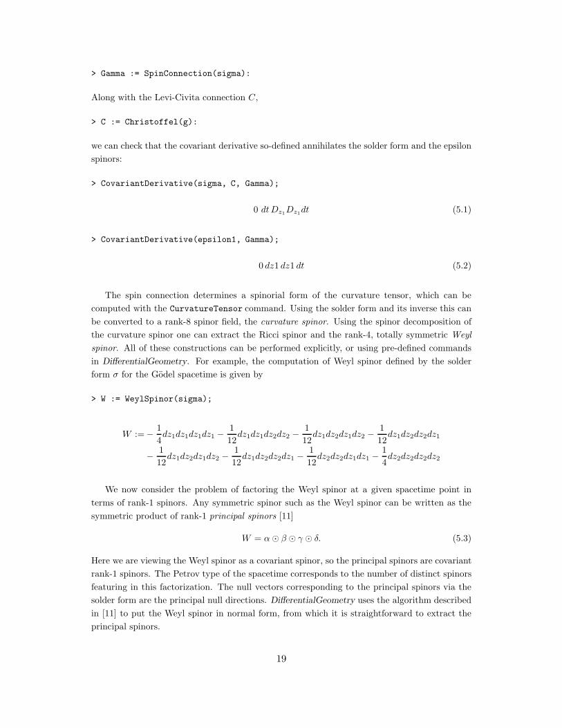
The spin connection determines a spinorial form of the curvature tensor, which can be

computed with the CurvatureTensor command. Using the solder form and its inverse this can

be converted to a rank-8 spinor field, the curvature spinor. Using the spinor decomposition of

the curvature spinor one can extract the Ricci spinor and the rank-4, totally symmetric Weyl

spinor. All of these constructions can be performed explicitly, or using pre-defined commands

in DifferentialGeometry. For example, the computation of Weyl spinor defined by the solder

form σ for the Godel spacetime is given by

> W := WeylSpinor(sigma);

W :=− 1

4dz1dz1dz1dz1 −

1

12dz1dz1dz2dz2 −

1

12dz1dz2dz1dz2 −

1

12dz1dz2dz2dz1

− 1

12dz1dz2dz1dz2 −

1

12dz1dz2dz2dz1 −

1

12dz2dz2dz1dz1 −

1

4dz2dz2dz2dz2

We now consider the problem of factoring the Weyl spinor at a given spacetime point in

terms of rank-1 spinors. Any symmetric spinor such as the Weyl spinor can be written as the

symmetric product of rank-1 principal spinors [11]

W = α⊙ β ⊙ γ ⊙ δ. (5.3)

Here we are viewing the Weyl spinor as a covariant spinor, so the principal spinors are covariant

rank-1 spinors. The Petrov type of the spacetime corresponds to the number of distinct spinors

featuring in this factorization. The null vectors corresponding to the principal spinors via the

solder form are the principal null directions. DifferentialGeometry uses the algorithm described

in [11] to put the Weyl spinor in normal form, from which it is straightforward to extract the

principal spinors.

19

In our Godel example above, the Petrov type is D, so the Penrose normal form is in fact the

factorized form. The principal spinors are not, in general, unique. In the type D case we can

demand that the two distinct principal spinors form an oriented, normalized spinor dyad; this

reduces the number of possible spinors. The FactorWeylSpinor command produces in the type

D case a list consisting of possible sets of normalized principal spinors in the form [α, α, β, β]

and the overall numerical factor η such that the totally symmetric product is of the form:

W = η α⊙ α⊙ β ⊙ β. (5.4)

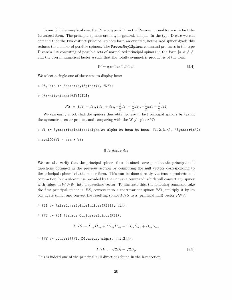
We select a single one of these sets to display here:

> PS, eta := FactorWeylSpinor(W, "D"):

> PS:=allvalues(PS[1])[2];

PS := [Idz1 + dz2, Idz1 + dz2,−1

2dz1 −

I

2dz2,−

1

2dz1− I

2dz2]

We can easily check that the spinors thus obtained are in fact principal spinors by taking

the symmetric tensor product and comparing with the Weyl spinor W :

> W1 := SymmetrizeIndices(alpha &t alpha &t beta &t beta, [1,2,3,4], "Symmetric"):

> evalDG(W1 - eta * W);

0 dz1dz1dz1dz1

We can also verify that the principal spinors thus obtained correspond to the principal null

directions obtained in the previous section by computing the null vectors corresponding to

the principal spinors via the solder form. This can be done directly via tensor products and

contraction, but a shortcut is provided by the Convert command, which will convert any spinor

with values in W ⊗W ′ into a spacetime vector. To illustrate this, the following command take

the first principal spinor in PS, convert it to a contravariant spinor PS1, multiply it by its

conjugate spinor and convert the resulting spinor PNS to a (principal null) vector PNV :

> PS1 := RaiseLowerSpinorIndices(PS[1], [1]):

> PNS := PS1 &tensor ConjugateSpinor(PS1);

PNS := Dz1Dw1+ IDz1Dw2

− IDz2Dw1+Dz2Dw2

> PNV := convert(PNS, DGtensor, sigma, [[1,2]]);

PNV :=√2Dt −

√2Dy (5.5)

This is indeed one of the principal null directions found in the last section.

20

6 Tensorial Invariants

Besides Killing vector fields there are a number of tensor fields whose existence can be used to

invariantly characterize spacetimes. Such tensor fields are discussed, e.g., in [2]. Here we consider

a few of these tensorial invariants and show how they can be computed via DifferentialGeometry.

6.1 Homothetic Vector Fields

A homothety of a spacetime (M, g) is a diffeomorphism φ : M → M and a constant c 6= 0 such

that

φ∗g = cg. (6.1)

A one parameter family of such diffeomorphisms is generated by a homothetic vector field V ,

which satisfies

LV g = (const.)g. (6.2)

Evidently, a Killing vector field is a special case of a homothetic vector field, and both are

special cases of a conformal Killing vector field. Modulo Killing vector fields, there is at most

one homothetic vector field (up to a scaling). A homothety is a scaling symmetry of the metric;

generic spacetime will admit no homotheties. Indeed, (6.2) represents an overdetermined system

of PDEs for V ; such systems are amenable to symbolic analysis.

As an example, we consider the plane wave spacetimes with metric given by

g = b(u) [a(u)du ⊗ du− P ′(u)Q′(u)du⊙ dv +Q′(u)dx⊗ dx+ P ′(u)dy ⊗ dy] , (6.3)

which is defined in DifferentialGeometry via

> DGsetup([u,v,x,y], M):

> g := evalDG(b(u) * (a(u)*du &t du - diff(P(u),u)*diff(Q(u),u)*du &s dv

+ diff(Q(u), u)*dx &t dx + diff(P(u),u)*dy &t dy):

Here a(u), b(u) > 0, P (u) and Q(u) are arbitrary functions such that P ′ > 0, Q′ > 0. Evaluation

of the Ricci tensor reveals that this is a vacuum spacetime for an appropriate choice of b(u),

which we shall not need to display.

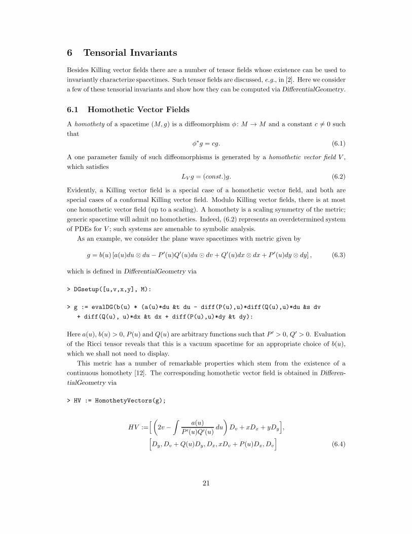
This metric has a number of remarkable properties which stem from the existence of a

continuous homothety [12]. The corresponding homothetic vector field is obtained in Differen-

tialGeometry via

> HV := HomothetyVectors(g);

HV :=[

(

2v −∫

a(u)

P ′(u)Q′(u)du

)

Dv + xDx + yDy

]

,

[

Dy, Dv +Q(u)Dy, Dx, xDv + P (u)Dx, Dv

]

(6.4)

21

The output of HomothetyVectors is a pair of lists. The first list contains a non-trivial homo-

thetic vector field (if any). The second list gives a basis for the vector space of Killing vector

fields. Together, the two lists provide a basis for the infinitesimal generators of the homothety

group. For the plane wave metric (6.3) we see that the homothety group of this spacetime is

6-dimensional and is defined by the choice of functions P and Q.

The corresponding 1-parameter family of homotheties can be computed using the Differen-

tialGeometry Flow command. The output is a list of equations specifying the diffeomorphisms.

The one parameter family of homotheties generated by the first vector field in HVF is given by:

> phi := Flow(HV[1][1], s);

φ :=

[

u = u, v = e2sv +1

2(1 − e2s)

∫

a(u)

Q′(u)du, x = esx, y = esy

]

(6.5)

This can be verified explicitly by checking φ∗g − e2sg = 0:

> Pullback(phi, g) &minus (exp(2*s) &mult g);

0 dudu

6.2 Killing Tensors and Killing-Yano Tensors

Killing tensors are generalizations of Killing vectors. A Killing tensor on a spacetime (M, g) is

a symmetric tensor, Ka1...ap= K(a1...ap), satisfying

∇(aKb1...bp) = 0, (6.6)

where ∇ is the connection on M compatible with g. Note that a Killing tensor of rank-1 is just

the 1-form corresponding via g to a Killing vector field. The metric g is always a Killing tensor

of rank 2.

A Killing-Yano tensor is a skew tensor, Ya1...ap= Y[a1...ap], satisfying

∇(aYb1)...bp = 0. (6.7)

We note that if Yab is a rank-2 Killing-Yano tensor then its square

Kab = YacYcb (6.8)

is a Killing tensor.

As with the equations for a Killing vector field or a homothetic vector field, the equations

defining Killing tensors and Killing-Yano tensors are overdetermined; generic spacetimes admit

no such tensors. The overdetermined nature of the equations makes them very amenable to

analysis using the symbolic PDE solving routines. As an example, we compute the rank 2

Killing-Yano tensor for the Kerr spacetime. This tensor and its corresponding Killing tensor

22

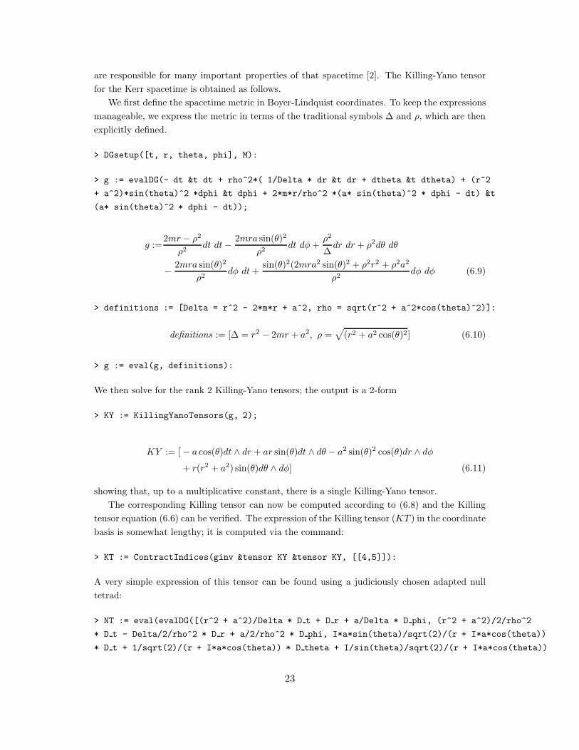
are responsible for many important properties of that spacetime [2]. The Killing-Yano tensor

for the Kerr spacetime is obtained as follows.

We first define the spacetime metric in Boyer-Lindquist coordinates. To keep the expressions

manageable, we express the metric in terms of the traditional symbols ∆ and ρ, which are then

explicitly defined.

> DGsetup([t, r, theta, phi], M):

> g := evalDG(- dt &t dt + rho^2*( 1/Delta * dr &t dr + dtheta &t dtheta) + (r^2

+ a^2)*sin(theta)^2 *dphi &t dphi + 2*m*r/rho^2 *(a* sin(theta)^2 * dphi - dt) &t

(a* sin(theta)^2 * dphi - dt));

g :=2mr − ρ2

ρ2dt dt− 2mra sin(θ)2

ρ2dt dφ+

ρ2

∆dr dr + ρ2dθ dθ

− 2mra sin(θ)2

ρ2dφ dt+

sin(θ)2(2mra2 sin(θ)2 + ρ2r2 + ρ2a2

ρ2dφ dφ (6.9)

> definitions := [Delta = r^2 - 2*m*r + a^2, rho = sqrt(r^2 + a^2*cos(theta)^2)]:

definitions := [∆ = r2 − 2mr + a2, ρ =√

(r2 + a2 cos(θ)2] (6.10)

> g := eval(g, definitions):

We then solve for the rank 2 Killing-Yano tensors; the output is a 2-form

> KY := KillingYanoTensors(g, 2);

KY := [− a cos(θ)dt ∧ dr + ar sin(θ)dt ∧ dθ − a2 sin(θ)2 cos(θ)dr ∧ dφ

+ r(r2 + a2) sin(θ)dθ ∧ dφ] (6.11)

showing that, up to a multiplicative constant, there is a single Killing-Yano tensor.

The corresponding Killing tensor can now be computed according to (6.8) and the Killing

tensor equation (6.6) can be verified. The expression of the Killing tensor (KT ) in the coordinate

basis is somewhat lengthy; it is computed via the command:

> KT := ContractIndices(ginv &tensor KY &tensor KY, [[4,5]]):

A very simple expression of this tensor can be found using a judiciously chosen adapted null

tetrad:

> NT := eval(evalDG([(r^2 + a^2)/Delta * D t + D r + a/Delta * D phi, (r^2 + a^2)/2/rho^2

* D t - Delta/2/rho^2 * D r + a/2/rho^2 * D phi, I*a*sin(theta)/sqrt(2)/(r + I*a*cos(theta))

* D t + 1/sqrt(2)/(r + I*a*cos(theta)) * D theta + I/sin(theta)/sqrt(2)/(r + I*a*cos(theta))

23

* D phi,-I*a*sin(theta)/sqrt(2)/(r - I*a*cos(theta)) * D t + 1/sqrt(2)/(r - I*a*cos(theta))

* D theta - I/sin(theta)/sqrt(2)/(r - I*a*cos(theta)) * D phi]), definitions):

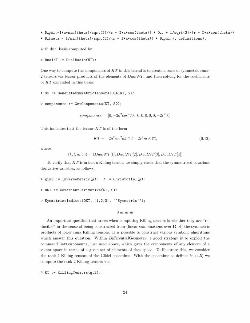
with dual basis computed by

> DualNT := DualBasis(NT):

One way to compute the components of KT in this tetrad is to create a basis of symmetric rank-

2 tensors via tensor products of the elements of DualNT , and then solving for the coefficients

of KT expanded in this basis:

> S2 := GenerateSymmetricTensors(DualNT, 2):

> components := GetComponents(KT, S2);

components := [0,−2a2cos2θ, 0, 0, 0, 0, 0, 0,−2r2, 0]

This indicates that the tensor KT is of the form

KT = −2a2cos2θk ⊙ l − 2r2m⊙m, (6.12)

where

(k, l,m,m) = (DualNT [1], DualNT [2], DualNT [3], DualNT [4])

To verify that KT is in fact a Killing tensor, we simply check that the symmetrized covariant

derivative vanishes, as follows.

> ginv := InverseMetric(g): C := Christoffel(g):

> DKT := CovariantDerivative(KT, C):

> SymmetrizeIndices(DKT, [1,2,3], ‘‘Symmetric’’);

0 dt dt dt

An important question that arises when computing Killing tensors is whether they are “re-

ducible” in the sense of being constructed from (linear combinations over R of) the symmetric

products of lower rank Killing tensors. It is possible to construct various symbolic algorithms

which answer this question. Within DifferentialGeometry, a good strategy is to exploit the

command GetComponents, just used above, which gives the components of any element of a

vector space in terms of a given set of elements of that space. To illustrate this, we consider

the rank 2 Killing tensors of the Godel spacetime. With the spacetime as defined in (4.5) we

compute the rank-2 Killing tensors via

> KT := KillingTensors(g,2):

24

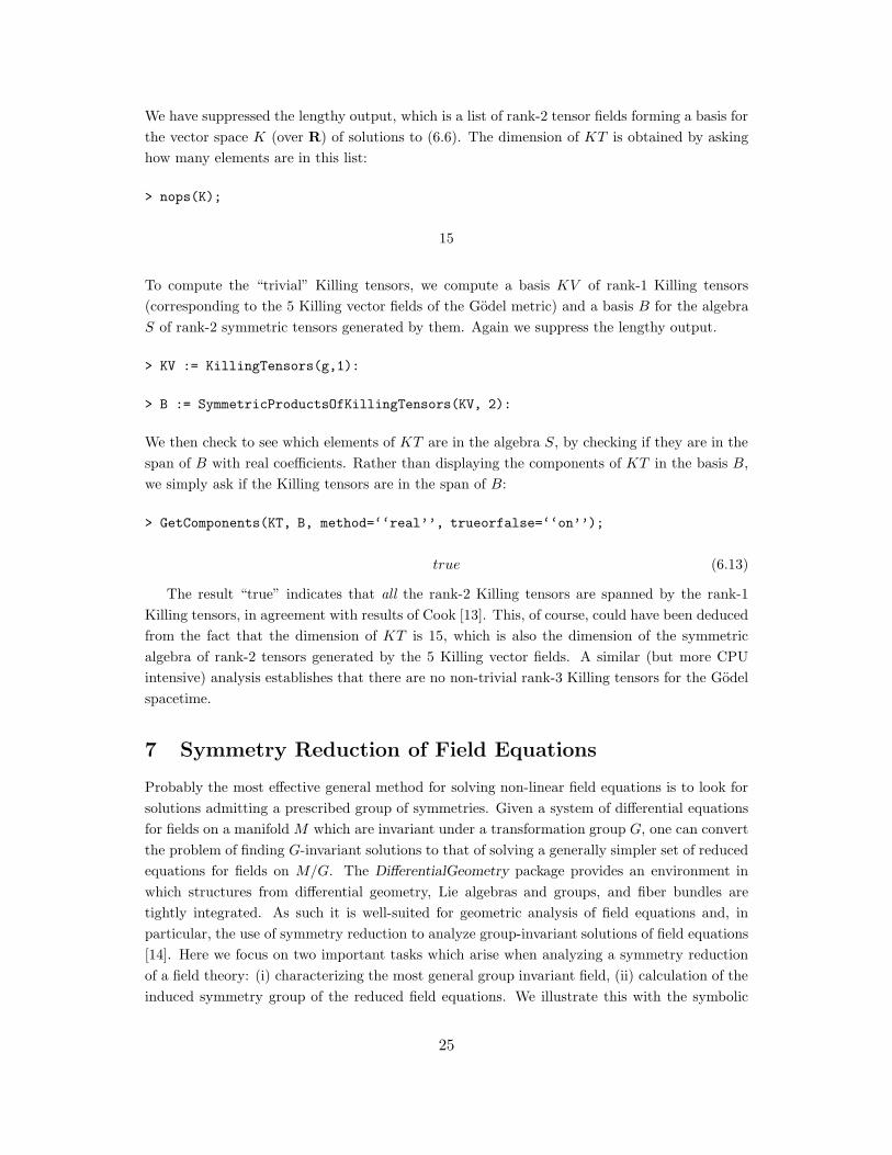
We have suppressed the lengthy output, which is a list of rank-2 tensor fields forming a basis for

the vector space K (over R) of solutions to (6.6). The dimension of KT is obtained by asking

how many elements are in this list:

> nops(K);

15

To compute the “trivial” Killing tensors, we compute a basis KV of rank-1 Killing tensors

(corresponding to the 5 Killing vector fields of the Godel metric) and a basis B for the algebra

S of rank-2 symmetric tensors generated by them. Again we suppress the lengthy output.

> KV := KillingTensors(g,1):

> B := SymmetricProductsOfKillingTensors(KV, 2):

We then check to see which elements of KT are in the algebra S, by checking if they are in the

span of B with real coefficients. Rather than displaying the components of KT in the basis B,

we simply ask if the Killing tensors are in the span of B:

> GetComponents(KT, B, method=‘‘real’’, trueorfalse=‘‘on’’);

true (6.13)

The result “true” indicates that all the rank-2 Killing tensors are spanned by the rank-1

Killing tensors, in agreement with results of Cook [13]. This, of course, could have been deduced

from the fact that the dimension of KT is 15, which is also the dimension of the symmetric

algebra of rank-2 tensors generated by the 5 Killing vector fields. A similar (but more CPU

intensive) analysis establishes that there are no non-trivial rank-3 Killing tensors for the Godel

spacetime.

7 Symmetry Reduction of Field Equations

Probably the most effective general method for solving non-linear field equations is to look for

solutions admitting a prescribed group of symmetries. Given a system of differential equations

for fields on a manifold M which are invariant under a transformation group G, one can convert

the problem of finding G-invariant solutions to that of solving a generally simpler set of reduced

equations for fields on M/G. The DifferentialGeometry package provides an environment in

which structures from differential geometry, Lie algebras and groups, and fiber bundles are

tightly integrated. As such it is well-suited for geometric analysis of field equations and, in

particular, the use of symmetry reduction to analyze group-invariant solutions of field equations

[14]. Here we focus on two important tasks which arise when analyzing a symmetry reduction

of a field theory: (i) characterizing the most general group invariant field, (ii) calculation of the

induced symmetry group of the reduced field equations. We illustrate this with the symbolic

25

analysis of the problem of finding gravitational plane waves, which can be defined as vacuum

spacetimes admitting a particular class of 5 dimensional isometry groups (see [12], and references

therein).

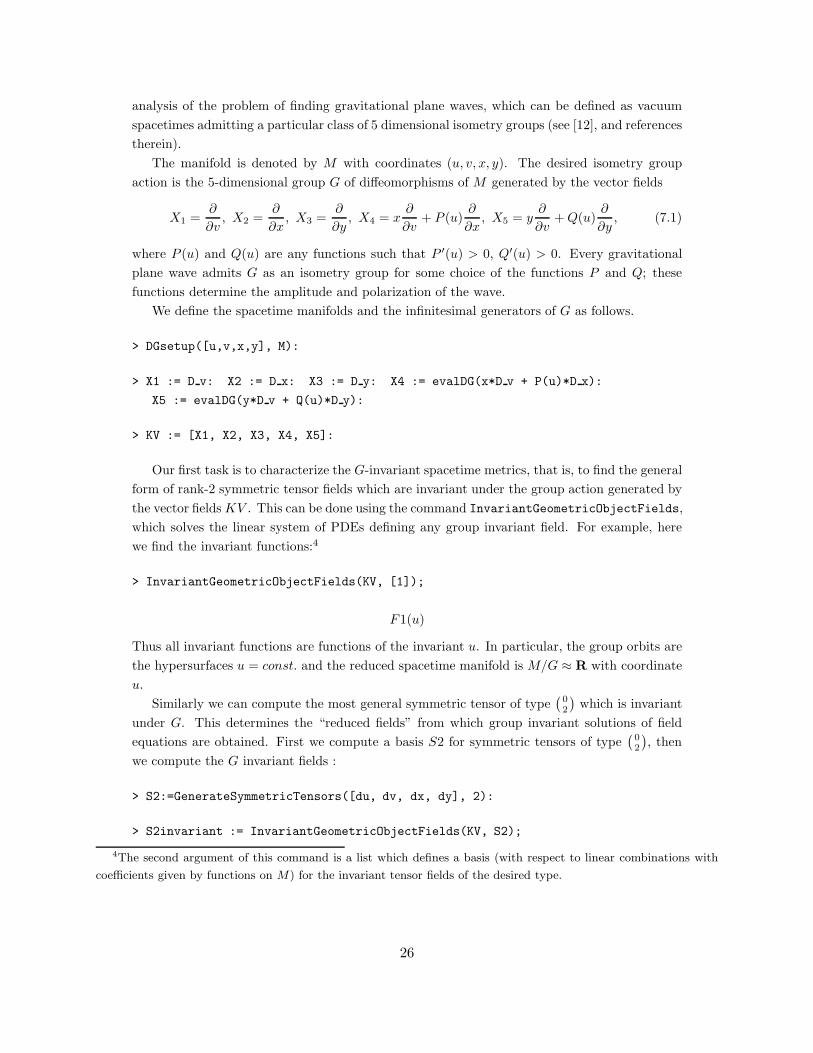
The manifold is denoted by M with coordinates (u, v, x, y). The desired isometry group

action is the 5-dimensional group G of diffeomorphisms of M generated by the vector fields

X1 =∂

∂v, X2 =

∂

∂x, X3 =

∂

∂y, X4 = x

∂

∂v+ P (u)

∂

∂x, X5 = y

∂

∂v+Q(u)

∂

∂y, (7.1)

where P (u) and Q(u) are any functions such that P ′(u) > 0, Q′(u) > 0. Every gravitational

plane wave admits G as an isometry group for some choice of the functions P and Q; these

functions determine the amplitude and polarization of the wave.

We define the spacetime manifolds and the infinitesimal generators of G as follows.

> DGsetup([u,v,x,y], M):

> X1 := D v: X2 := D x: X3 := D y: X4 := evalDG(x*D v + P(u)*D x):

X5 := evalDG(y*D v + Q(u)*D y):

> KV := [X1, X2, X3, X4, X5]:

Our first task is to characterize the G-invariant spacetime metrics, that is, to find the general

form of rank-2 symmetric tensor fields which are invariant under the group action generated by

the vector fieldsKV . This can be done using the command InvariantGeometricObjectFields,

which solves the linear system of PDEs defining any group invariant field. For example, here

we find the invariant functions:4

> InvariantGeometricObjectFields(KV, [1]);

F1(u)

Thus all invariant functions are functions of the invariant u. In particular, the group orbits are

the hypersurfaces u = const. and the reduced spacetime manifold is M/G ≈ R with coordinate

u.

Similarly we can compute the most general symmetric tensor of type(

02

)

which is invariant

under G. This determines the “reduced fields” from which group invariant solutions of field

equations are obtained. First we compute a basis S2 for symmetric tensors of type(

02

)

, then

we compute the G invariant fields :

> S2:=GenerateSymmetricTensors([du, dv, dx, dy], 2):

> S2invariant := InvariantGeometricObjectFields(KV, S2);

4The second argument of this command is a list which defines a basis (with respect to linear combinations with

coefficients given by functions on M) for the invariant tensor fields of the desired type.

26

S2invariant :=F1(u)(

− d

duP (u)

d

duQ(u)(du dv + dv du) +

d

duQ(u)dx dx+

d

duP (u)dy dy

)

+ F2(u)du du (7.2)

Thus the set of G-invariant symmetric tensors of type(

02

)

is spanned by two quadratic forms:

Q1 = du ⊗ du, Q2 = −Q′(u)P ′(u)du⊙ dv +Q′(u)dx⊗ dx+ P ′(u)dy ⊗ dy. (7.3)

The most general G-invariant metric takes the form

g = a(u)Q1 + b(u)Q2, (7.4)

where b(u) > 0. The symmetry reduced fields on M/G ≈ R are a(u) and b(u).

One obtains symmetry reduced equations for a(u) and b(u) by substituting (7.4) into the

relevant field equations, e.g., the Einstein equations. Generally covariant field equations such as

the Einstein equations have the group Diff(M) of diffeomorphisms of M (acting by pull-back on

the metric) as a symmetry group. The full group of diffeomorphisms does not act on the space

of metrics (7.4) so Diff(M) cannot be a symmetry group of the symmetry reduced equations.

The subgroup of Diff(M) which does act on the G-invariant metrics and which will also be a

symmetry group of the reduced equations is the normalizer of G within Diff(M) [14]. Thus

the normalizer is the residual symmetry group after symmetry reduction. The normalizer of G

in Diff(M) is the smallest subgroup of Diff(M) containing G as a normal subgroup. Working

infinitesimally, the Lie algebra of the normalizer can be computed as the smallest algebra of

vector fields containing the isometry algebra generated by KV as an ideal. These vector fields

are obtained by solving a large system of linear PDEs which are amenable to symbolic analysis.

TheDifferentialGeometrycommand InfinitesimalPseudoGroupNormalizer solves these PDEs

and thus computes the Lie algebra of the normalizer within the Lie algebra of all vector fields.5

In the present example we get

> Nor := InfinitesimalPseudoGroupNormalizer(KV);

Nor := (2C1 v + F1(u))Dv + C1 xDx + C1 yDy

Thus the residual symmetry group consists of a scaling of (v, x, y) and a u dependent translation

of v. These transformations can be computed explicitly using the DifferentialGeometry Flow

command as follows. First, for simplicity, we break the vector field Nor into its translational

and scaling parts, respectively:

> NorTrans := eval(Nor, C1=0, F1(u) = f(u));

NorTrans := f(u)Dv

5The default for this computation is to compute the normalizer within the set Γ of all vector fields. Other choices

for Γ can be made.

27

> NorScale := eval(Nor, C1=1, F1(u) = 0);

NorScale := 2v Dv + xDx + yDy

Then we compute each of the flows using parameters α and β respectively. The result is two

sets of transformations, specified as relations between the original and transformed coordinate

values:

> Trans := Flow(NorTrans, alpha);

Trans := [u = u, v = v + αf(u), x = x, y = y]

> Scale := Flow(NorScale, beta);

Trans := [u = u, v = e2βv, x = eβx, y = eβy]

Any generally covariant field theory (not just general relativity, or a theory of a metric) will

admit these transformations as symmetries upon symmetry reduction by the symmetry group

defined by (7.1).

We can verify that the residual symmetry group does indeed act on the G-invariant metric

(7.4) via the Pullback command. Defining Q1 and Q2 as in (7.3) we have

> Pullback(Trans, Q1);

du du

> Pullback(Trans, Q2)

−2αdP (u)

du

dQ(u)

u

df(u)

udu du− dP (u)

du

dQ(u)

du(du dv + dv du) +

dQ(u)

dudx dx+

dP (u)

dudy dy

> Pullback(Scale, Q1);

du du

> Pullback(Scale, Q2);

e2β(−dP (u)

du

dQ(u)

du(du dv + dv du) +

dQ(u)

dudx dx +

dP (u)

dudy dy)

Thus the action of the residual group on the functions (a(u), b(u)) defining the G-invariant

metrics can be expressed as

a(u) −→ a(u)− 2αP ′(u)Q′(u)f ′(u)b(u), b(u) −→ e2βb(u). (7.5)

From this action of the residual symmetry group we see that the function a(u) can be “gauged”

to zero via Trans. We can also see that, with an appropriate choice of f(u), the residual group

includes a homothety of the metric (7.4), as discussed in §6.1.

28

References

[1] M. MacCallum, J. Skea, R, McLenaghan, J. McCrea, Algebraic Computing in General Rela-

tivity: Lecture Notes from the First Brazilian School on Computer Algebra, Volume 2, Oxford

University Press (1995).

[2] H. Stephani, D. Kramer, M. MacCallum, C. Hoenselaers, E. Herlt, Exact Solutions of Ein-

stein’s Field Equations, Cambridge University Press (2003).

[3] A. Heck, Introduction to Maple, Springer (2003).

[4] A. Ashtekar and A. Magnon-Ashtekar J. Math. Phys. 19, 1567–1572 (1978).

[5] J. Patera, P. Winternitz, H. Zassenhaus, J. Math. Phys. 16, 1597–1614 (1975).

[6] S. Kobayashi and K. Nomizu, Foundations of Differential Geometry, Volume II, Wiley

(1969).

[7] W. Kundt, Z. Phys. 163, 77 (1961).

[8] We thank Dillon Morse for this example.

[9] M. Acvevedo, M. Enciso-Aguilar, J. Lopez-Bonilla, Electron. J. Theor. Physics 9, 79 (2006).

[10] E. Zakhary and J. Carminati, Gen. Rel. Grav. 36, 1015 (2004).

[11] R. Penrose and W. Rindler, Spinors and Spacetime, Volume II, Cambridge University Press

(1984).

[12] C. G. Torre, Gen. Rel. Grav. 38, 653 (2006).

[13] S. Cook, Killing Spinors and Affine Symmetry Tensors in Godel’s Universe, PhD disserta-

tion, Oregon State University (2009).

[14] I. Anderson, M. Fels, C. G. Torre, Commun. Math. Phys. 212, 653 (2000).

A DifferentialGeometry Commands

The following is a list of all commands in DifferentialGeometry and its various sub-packages.

A.1 DifferentialGeometry package

• &minus: find the difference between two vectors, differential forms or tensors.

• &mult: multiply a vector, differential form or tensor by a Maple expression.

• &plus: add two vectors, differential forms or tensors.

• &tensor: calculate the tensor product of two tensors.

29

• &wedge: calculate the exterior product of two differential forms.

• Annihilator: find the subspace of vectors (or 1-forms) whose interior product with a given

list of 1-forms (vectors) vanish.

• ApplyTransformation: evaluate a transformation at a point.

• ChangeFrame: change the current or active frame.

• ComplementaryBasis: extend a basis for subspace to a basis for larger subspace.

• ComposeTransformations: compose a sequence of two or more transformations.

• Convert: change the presentations of various geometric objects.

• DeRhamHomotopy: the homotopy operator for the exterior derivative operator (the de

Rham complex).

• DGbasis: select a maximal linearly independent list of elements from a list of vectors,

forms or tensors.

• DGsetup: initialize a coordinate system, frame, or Lie algebra.

• DGzip: form a linear combination, wedge product or tensor product of a list of vectors,

forms or tensors.

• DualBasis: calculate the dual basis to a given basis of vectors or 1-forms.

• evalDG: evaluate a DifferentialGeometry expression.

• ExteriorDerivative: take the exterior derivative of a differential form.

• Flow: calculate the 1-parameter group of diffeomorphisms (the flow) of a vector field.

30

• FrameData: calculate the structure equations for a generic (anholomonic) frame.

• GroupActions: a package for Lie groups and group actions on manifolds.

• Hook: the interior product of a vector or a list of vectors with a differential form.

• InfinitesimalTransformation: compute the Lie algebra of infinitesimal generators for an

action of a Lie group on a manifold.

• IntegrateForm: evaluate a p-fold iterated integral of a differential p-form.

• IntersectSubspaces: find the intersection of a list of vector subspaces of vectors, forms or

tensors.

• InverseTransformation: find the inverse of a transformation.

• JetCalculus: a package for the variational calculus on jet spaces.

• Library: a package of databases of Lie algebras, vector field systems, and differential

equations.

• LieAlgebras: a package for the symbolic analysis of Lie algebras.

• LieBracket: calculate the Lie bracket of two vector fields.

• LieDerivative: calculate the Lie derivative of a vector field, differential form or tensor with

respect to a vector field.

• GetComponents: find the coefficients of a vector, differential form or tensor with respect

to a list of vectors, differential forms or tensors.

• Preferences: set worksheet preferences for the DifferentialGeometry package.

31

• Pullback: pullback a differential p-form by the Jacobian of a transformation.

• PullbackVector: find (if possible) a vector field whose pushforward by the Jacobian of a

given transformation is a given vector field.

• Pushforward: pushforward a vector or a vector field by the Jacobian of a transformation.

• RemoveFrame: remove a frame from a Maple session.

• Tensor: a package for tensor analysis within the DifferentialGeometry environment.

• Tools: a small utility package for DifferentialGeometry .

• Transformation: create a transformation or mapping from one manifold to another.

A.2 GroupActions sub-package

• Action: find the action of a solvable Lie group on a manifold from its infinitesimal gener-

ators.

• InfinitesimalSymmetriesOfGeometricObjectFields: find the infinitesimal symmetries (vec-

tor fields) for a collection of vector fields, differential forms or tensors.

• InvariantGeometricObjectFields: find the vector fields, differential forms, or tensors which

are invariant with respect to a Lie algebra of vector fields.

• InvariantVectorsAndForms: calculate a basis of left and right invariant vector fields and

differential 1-forms on a Lie group.

• IsotropyFilteration: find the infinitesimal isotropy filtration for a Lie algebra of vector

fields.

32

• IsotropySubalgebra: find the infinitesimal isotropy subalgebra of a Lie algebra of vector

fields and infinitesimal isotropy representation.

• LieGroup: create a module defining a Lie group.

• LiesThirdTheorem: find a Lie algebra of pointwise independent vector fields with pre-

scribed structure equations (solvable algebras only).

• MovingFrames: a small package for the method of moving frames.

A.3 JetCalculus sub-package

• AssignTransformationType: assign a type (projectable, point, contact, ...) to a transfor-

mation.

• AssignVectorType: assign a type (projectable, point, contact, ...) to a vector.

• DifferentialEquationData: create a data structure for a system of differential equations.

• EulerLagrange: calculate the Euler-Lagrange equations for a Lagrangian.

• EvolutionaryVector: find the evolutionary part of a vector field.

• GeneralizedLieBracket: find the Lie bracket of two generalized vector fields.

• GeneratingFunctionToContactVector: find the contact vector field defined by a generating

function.

• HigherEulerOperators: apply the higher Euler operators to a function or a differential

bi-form.

• HorizontalExteriorDerivative: calculate the horizontal exterior derivative of a bi-form on

a jet space.

33

• HorizontalHomotopy: apply the horizontal homotopy operator to a bi-form on a jet space.

• IntegrationByParts: apply the integration by parts operator to a differential bi-form.

• Noether: find the conservation law for the Euler-Lagrange equations from a given symme-

try of the Lagrangian

• ProjectedPullback: pullback a differential bi-form of type (r, s)by a transformation to a

differential bi-form of type (r, s).

• ProjectionTransformation: construct the canonical projection map between jet spaces of

a fiber bundle.

• Prolong: prolong a jet space, vector field, transformation, or differential equation to a

higher order jet space.

• PushforwardTotalVector: pushforward a total vector field by a transformation.

• TotalDiff: take the total derivative of an expression, a differential form or a contact form.

• TotalJacobian: find the Jacobian of a transformation using total derivatives.

• TotalVector: find the total part of a vector field.

• VerticalExteriorDerivative: calculate the vertical exterior derivative of a bi-form on a jet

space.

• VerticalHomotopy: apply the vertical homotopy operator to a bi-form on a jet space.

• ZigZag: lift a dHclosed form on a jet space to a dclosed form.

A.4 LieAlgebras sub-package

34

• Adjoint: find the Adjoint Matrix for a vector in a Lie algebra.

• AdjointExp: find the Exponential of the Adjoint Matrix for a vector in a Lie algebra.

• ApplyHomomorphism: apply a Lie algebra homomorphism to a vector, form or tensor.

• BracketOfSubspaces: find the subspace generated by the bracketing of two subspaces.

• Center: find the center of a Lie algebra.

• Centralizer: find the centralizer of a list of vectors.

• ChangeLieAlgebraTo: change the current frame to the frame for a Lie algebra.

• Complexify: find the complexification of a Lie algebra.

• Decompose: decompose a Lie algebra into a direct sum of indecomposable Lie algebras.

• Derivations: find the inner and/or Outer derivations of a Lie algebra.

• DerivedAlgebra: find the derived algebra of a Lie algebra.

• DirectSum: create the direct sum of a list of Lie algebras.

• Extension: calculate a right or a central extension of a Lie algebra.

• GeneralizedCenter: calculate the generalized center of an ideal in a Lie algebra.

• HomomorphismSubalgebras: find the kernel or image of a Lie algebra homomorphism.

• JacobsonRadical: find the Jacobson radical for a matrix Lie algebra.

35

• Killing: find the Killing form of a Lie algebra.

• LeviDecomposition: compute the Levi decomposition of a Lie algebra.

• LieAlgebraCohomology: a package for computing Lie algebra cohomology.

• LieAlgebraData: convert different realizations of a Lie algebra to a Lie algebra data struc-

ture.

• LieAlgebraRepresentations: a package for the symbolic analysis of representations of Lie

algebras.

• MatrixAlgebras: create a Lie algebra data structure for a matrix Lie algebra.

• MatrixCentralizer: find the matrix centralizer of a list of matrices.

• MinimalIdeal: find the smallest ideal containing a given set of vectors.

• MinimalSubalgebra: find the smallest ideal containing a given set of vectors.

• MultiplicationTable: display the multiplication table of a Lie algebra.

• Nilradical: find the nilradical of a Lie algebra.

• Query: check various properties of a Lie algebra, subalgebra, or transformation.

• QuotientAlgebra: create the Lie algebra data structure for a quotient algebra of a Lie

algebra by an ideal.

• Radical: find the radical of a Lie algebra.

• SemiDirectSum: create the semi-direct product of two Lie algebras.

36

• Series: find the derived series, lower central series, upper central series of a Lie algebra or

a Lie subalgebra.

• SubalgebraNormalizer: find the normalizer of a subalgebra.

A.5 Tensor sub-package

Commands for the algebraic manipulation of tensors

• CanonicalTensors: create various standard tensors.

• ContractIndices: contract the indices of a tensor.

• Convert/DGspinor: convert a tensor to a spinor.

• Convert/DGtensor: convert an array, vector, p-form, spinor ... to a tensor.

• DGGramSchmidt: construction an orthonormal basis of vector, forms, tensors with respect

to a metric.

• GenerateSymmetricTensors: generate a list of symmetric tensors from a list of tensors.

• GenerateTensors: generate a list of tensors from a list of lists of tensors.

• HodgeStar: apply the Hodge star operator to a differential form.

• InverseMetric: find the inverse of a metric tensor.

• KroneckerDelta: find the Kronecker delta tensor of rank r.

• MetricDensity: use a metric tensor to create a scalar density of a given weight.

• MultiVector: compute the alternating sum of the tensor product of a list of vector fields.

37

• PermutationSymbol: create a permutation symbol.

• PushPullTensor: transform a tensor from one manifold or coordinate system to another.

• RaiseLowerIndices: raise or lower a list of indices of a tensor.

• RearrangeIndices: rearrange the argument/indices of a tensor.

• SymmetrizeIndices: symmetrize or skew-symmetrize a list of tensor indices.

• TensorInnerProduct: compute the inner product of two vectors, forms or tensors with

respect to a given metric tensor.

Commands for tensor differentiation

• Christoffel: find the Christoffel symbols of the first or second kind for a metric tensor.

• Connection: define a linear connection on the tangent bundle or on a vector bundle.

• CovariantDerivative: calculate the covariant derivative of a tensor field with respect to a

connection.

• DirectionalCovariantDerivative: calculate the covariant derivative of a tensor field in the

direction of a vector field and with respect to a given connection

• GeodesicEquations: calculate the geodesic equations for a symmetric linear connection on

the tangent bundle .

• Laplacian: find the Laplacian of a differential form with respect to a metric.

• ParallelTransportEquations: calculate the parallel transport equations for a linear connec-

tion on the tangent bundle or a linear connection on a vector bundle.

• TensorBrackets: calculate the Schouten bracket and Frolicher-Nijenhuis brackets of tensor

fields.

38

• TorsionTensor: calculate the torsion tensor for a linear connection on the tangent bundle.

Commands for calculating curvature tensors

• Christoffel: find the Christoffel symbols of the first or second kind for a metric tensor.

• Connection: define a linear connection on the tangent bundle or on a vector bundle.

• CottonTensor: calculate the Cotton tensor for a metric.

• CurvatureTensor: calculate the curvature tensor of a linear connection on the tangent

bundle or on a vector bundle.

• EinsteinTensor: calculate the Einstein tensor for a metric.

• RicciScalar: calculate the Ricci scalar for a metric.

• RicciTensor: calculate the Ricci tensor of a linear connection on the tangent bundle.

• RiemannInvariants: calculate a complete set of scalar curvature invariants in 4 dimensions.

• SectionalCurvature: calculate the sectional curvature for a metric.

• WeylTensor: calculate the Weyl curvature tensor of a metric.

Commands for calculating special tensor fields

• CovariantlyConstantTensors: calculate the covariantly constant tensors with respect to a

given metric or connection.

• KillingSpinors: calculate the Killing spinors for a given spacetime.

• KillingYanoTensors: calculate the Killing tensors of a specified rank for a given metric or

connection.

39

• KillingTensors: calculate the Killing-Yano tensors for a given connection or a given metric.

• RecurrentTensors: calculate the recurrent tensors with respect to a given metric or con-

nection.

Commands for working with Killing tensors

• CheckKillingTensor: check that a tensor is the Killing tensor for a metric.

• IndependentKillingTensors: create a list of linearly independent Killing tensors.

• KillingBracket: a covariant form of the Schouten bracket for symmetric tensors.

• SymmetricProductsOfKillingTensors: form all possible symmetric tensors of a given rank.

Commands for the 2-component spinor formalism

• BivectorSolderForm: calculate the rank 4 spin-tensor which maps bivectors to symmetric

rank 2 spinors.

• ConjugateSpinor: calculate the complex conjugate of a spinor.

• EpsilonSpinor: calculate the epsilon spinor in the 2 component spinor formalism.

• KroneckerDeltaSpinor: calculate the Kronecker delta spinor in the 2 component spinor

formalism.

• RaiseLowerSpinorIndices: raise/lower the indices of a spinor or spin-tensor using the ep-

silon spinors.

• RicciSpinor: calculate the rank 4 Ricci spinor corresponding to the trace-free Ricci tensor.

• SolderForm: calculate the solder form (or Infeld-van der Waerden symbols) from an or-

thonormal tetrad.

40

• SpinConnection: calculate the unique spin connection defined by a solder form.

• SpinorInnerProduct: contract all spinor indices of 2 spin-tensors using the epsilon spinors.

• WeylSpinor: calculate the rank 4 Weyl spinor corresponding to the Weyl tensor.

Commands for the Newman-Penrose formalism

• GRQuery: verify various properties of spacetimes.

• NPBianchiIdentities: calculate the Bianchi identities in the Newman-Penrose formalism.

• NPCurvatureScalars: calculate the Ricci scalars and the Weyl scalars in the Newman-

Penrose formalism.

• NPDirectionalDerivatives: define the directional derivative operators used in the Newman-

Penrose formalism.

• NPRicciIdentities: calculate the Ricci identities in the Newman-Penrose formalism.

• NPSpinCoefficients: calculate the Newman-Penrose spin coefficients.

• NullTetrad: calculate a null tetrad from an orthonormal tetrad.

• NullTetradTransformation: apply a Lorentz transformation to a null tetrad.

• OrthonormalTetrad: calculate an orthonormal tetrad from a null tetrad.

• SpacetimeConventions: a description of the tensor and spinor conventions used by the

DifferentialGeometry package.

Commands for the algebraic classification of spacetimes

• IsotropyType: determine the isotropy type of the isotropy subalgebra of infinitesimal

isometries.

41

• PetrovType: determine the Petrov type of a spacetime from the Weyl tensor.

• SegreType: determine the Plebanski-Petrov type and the Segre type of a trace-free, rank

2 symmetric tensor.

• SubspaceType: determine the signature of the metric restricted to a subspace.

Commands for calculation of tensorial invariants

• KillingBracket: a covariant form of the Schouten bracket for symmetric tensors.

• KillingSpinors: calculate the Killing spinors for a given spacetime.

• KillingTensors: calculate the Killing tensors of a specified rank for a given metric or

connection.

• KillingVectors: calculate the Killing vectors for a given metric.

• KillingYanoTensors: calculate the Killing-Yano tensors for a given connection or a given

metric.

Commands for field theory

• BelRobinson: calculate the rank 4 Bel-Robinson tensor for a metric.

• DivergenceIdentities: check the divergence identity for various energy-momentum tensors.

• EnergyMomentumTensor: calculate the energy-momentum tensor for various fields (scalar,

electromagnetic, dust, ...).

• MatterFieldEquations: calculate the field equations for various field theories (scalar, elec-

tromagnetic, dust, ...).

42