New Arguments for the Discussion on the Fiscal Incentives to the

Accumulation of Human Capital and the Economic Growth. *

Jaime Alonso-Carrera

andMaría Jesús Freire-Serén

Universidade de Vigo, Facultade de Ciencias Económicas.

As Lagoas Marcosende s/n, 36200 Vigo, Spain.Phone: +34 986 812 504, Fax: +34 986 812401.

e-mail: jalonso@uvigo.es.

October 1999

(A very preliminary version)

* We are indebted to Xavier Raurich for his very useful discussions and comments. Of course, all errors thatremain are entirely our own. This paper was partially written during our visiting to the Department of Economicsat the University of Pennsylvania. María Jesús Freire-Serén acknowledges the financial support from FundaciónPROVIGO.

2

New Arguments for the Discussion on the Fiscal Incentives to the

Accumulation of Human Capital and the Economic Growth.

Abstract

This paper presents a three-sector model of endogenous growth with physical and human capital

accumulation. We integrated the two extreme approaches used in the preceding literature to design

the process of human capital accumulation. In this paper, the accumulation of human capital is a

home production in which individuals combines their non-working time with market educational

goods. This new characterization of human capital accumulation provides a framework that permits

a complete fiscal policy analysis. Unlike the preceding literature, we can analyze how fiscal policy

affects to all individuals’ margins of decision regarding to human capital accumulation. We obtain

that the way in which individuals combine educational goods and schooling time determines the

impact that fiscal policy has in both the stability property of the equilibrium and in the long-run

growth rate.

Keywords: Fiscal Policy, Human Capital, Economic Growth.

3

1. Introduction.

Since the seminal paper of Lucas (1988), human capital accumulation has been widely uses as an

engine of growth in the modern literature on economic growth. In this class of models, individuals

may devote part of their effort and resources to increase the efficiency units of labor they supply in

the labor market. The growth rate of income per capita is endogenously determined by interaction

among the technologies that allow for the accumulation of physical and human capital. In this

environment, the intervention of the government deserves an important role since the fiscal policy

can exhibit considerable growth effects. Several studies have examined the mechanisms by which

alternative fiscal policies affect the accumulation of human capital, and so the economic growth [see,

among others, Lucas (1990), Rebelo and Stokey (1995), Milesi-Ferretti and Roubini (1998)]. The

aim of the present paper is to provide new arguments and conclusions about the role that human

capital accumulation plays in driving the economic growth.

Traditionally, the endogenous growth models with human capital accumulation have considered

two alternative assumptions about the nature for the activity producing new human capital. The first

conception assumes that human capital accumulation is a home activity or a pure non-market

activity. Individuals allocate part of their endowments of physical capital and time to increase their

efficient units of labor at home. 1 The cost of accumulating human capital is then the market returns to

physical capital and time to which individuals forego when they devote these inputs to that activity.

However, while these inputs allocated in producing new human capital are not directly remunerated,

they will have an implicit compensation through the increase in the future labor earnings. Therefore,

the accumulation of human capital is an investment process that is not perfectly substitutive for

physical capital investment and consumption.

The second approach considers that the process of human capital accumulation is a pure market

activity. More precisely, there is a market sector supplying “educational goods” competitively.

1 Generally these models consider a human capital process that uses time in efficient units of labor as uniqueinput [See Lucas (1988)].

4

Individuals buy these goods to the firms so as to increase the efficiency of their labor [See, e.g.,

Rebelo and Stockey (1995) or Alonso-Carrera (1999)]. The educational goods directly raise the

efficiency units of labor without any additional manipulation. In other words, individuals do not need

any technology to transform these educational goods in new human capital. Thus, the accumulation

of human capital has only a direct cost that is given by the market price of the educational goods.

Therefore, the investment in human capital is now a perfect substitute for physical capital investment

and consumption.

The two previous approaches predict the same equilibrium dynamics and long-run growth rate.

Nevertheless, this indifference disappears when they are used to make fiscal policy analysis. On one

hand, as is pointed out by Milessi-Ferreti and Roubini (1998), the effects of fiscal policy crucially

depends on the nature of the activity accumulating human capital. Fiscal policy affects different

individuals’ margins of decision depending on whether the human capital accumulation is either a

pure market or a pure non-market activity. While in the first case the fiscal policies affect individuals’

purchases of educational goods, in the second they alter individuals’ allocation of time. On the other

hand, the chosen approach determines the menu of fiscal policies that can be analyzed. For instance,

the second approach must be used if we want to study the growth effect of a subsidy to the

purchases of educational goods. One must instead use the first approach to study the growth effects

of a fellowship that compensates the foregoing earnings. However, although the two previous fiscal

policies coexist in the reality, they cannot be jointly studied in a same model. Thus, none of the two

approaches are useful to analyze the cross effects between different fiscal policies. Therefore, the

use of one of these approaches to analyze the growth effects of alternative fiscal policies only permits

to obtain partial conclusions.

A complete fiscal policy analysis seems to require a framework where the process of human

capital accumulation would be designed by using microfoundations from the casual empiricism and

education economy. This paper builds a three-sector model where the accumulation of human

capital combines both educational goods and non-working time as was proposed by Becker

(1965). In particular, we integrate the two approaches described above. We assume that individuals

5

buy educational goods in the market, but to transform these goods in new human capital an

additional technology is required. The process of human capital accumulation is then a home

production in which individuals spends part of their time to manipulate these educational goods so as

to increase the efficiency units of their labor. For instance, we observe that students spend time in

using those educational goods (e.g., attendance the courses, the teachers’ time, libraries and

computer room) that they pay in the enrollment.

Our framework permits us to sum up both sides of the process of human capital accumulation,

and so it will be useful to develop complete fiscal policy analyses. The question that arises now is

how our technology of human capital accumulation affects the equilibrium dynamics, the long-run

growth rate and the growth effects of alternative fiscal policies. In particular, we will show that these

preceding two-sector growth models with human capital predicted too large growth rates. This

conclusion derives from our result showing that the growth rate is now a U-shaped function of the

elasticity of the productivity of schooling time with respect to educational goods. This result gives a

potential explanation of disparities in the per capita income growth across countries. Two identical

countries that are initially identical except for their time intensity in the technology of human capital

accumulation can growth at a different rate.

Moreover, our model also allows us to analyze a complete menu of fiscal policies that could alter

the accumulation of human capital. In particular, we include a tax on physical capital income, a tax

on human capital income, a subsidy to the purchases of educational goods and a subsidy to the

opportunity cost of schooling time.2 In presence of these fiscal instruments, the way in which

individuals combine educational goods and schooling time to obtain new human capital has two other

important consequences. On one hand, it determines the equilibrium dynamics. Under some

combination of the fiscal policy instruments, the equilibrium is locally indeterminate if the physical

capital intensity is larger in the sector producing educational goods than in the physical goods sector.

This result can be used to explain some unpredictable differences in the growth patterns followed by

totally identical economies [see, e.g., Benhabib and Farmer (1999)]. On the other hand, we get that

2 Note that the subsidy to the opportunity cost of schooling time was never studied before.

6

the tax on human capital income has a positive growth effect if the rate of the subsidy to the

opportunity cost of schooling time is sufficiently large. This result also arises in the approach that

considers the process of human capital accumulation as a pure non-market activity. However, in this

case the required rate of the subsidy to opportunity cost is much larger than in our model.

The paper is organized as follows. In Section 2 we present the model and define the competitive

equilibrium of the economy. Section 3 characterizes the equilibrium dynamics, analyzing the role that

the new technology of human capital accumulation and the fiscal polices play in determining the

dynamic behavior of the economy. In Section 4 we compute the long-run growth rate of the

economy and show how the relative participation of time in the accumulation of human capital

affects this growth rate. The growth effects of changes in the rates of the fiscal policies are analyzed

in Section 5. Section 6 concludes the paper.

2. The Model.

We consider an infinite horizon, continuous time, and endogenous growth model with physical

and human capital accumulation. The economy consists of competitive firms, a representative

household and a government. The competitive equilibrium is achieved by a decentralized manner

through perfect competition among firms and optimizing behavior by the household.

2.1 Production.

In our economy there are two types of firms which produce physical goods, )(tY , and

educational goods, )(tE , respectively. Physical goods are produced according to the Cobb-

Douglas technology ( ) ( ) β−β= 1)()()()()( thtutKtvAtY β= )()()( 1 tzthtAu , where 0>A is the scale

factor, )(tv and )(tu are respectively the shares of physical capital and human capital allocated to

the physical goods sector, and ( ) ( ))()()()()(1 thtutKtvtz = is the ratio of physical capital to labor

in efficiency units in the physical goods sector. Physical goods may be either used for consumption

or for investment in physical capital. In the sector producing educational goods, we also postulate a

7

Cobb-Douglas production function, with

( ) ( )( ) α−α −−= 1)()()()())(1()( thtutltKtvBtE ( ) α−= )()()()( 2 tzthtutlB , where 0>B is the

scale factor, and ( )( ) ( )( ))()()()()(1)(2 thtutltKtvtz −−= .

Let us denote the relative price of educational goods in units of physical goods, rental rate of

physical capital and rental rate of human capital by )(tp , )(tr and )(tw , respectively. Since firms

behave competitively, the value of the marginal productivity of each input is equal to its rental rate.

Hence, if both physical capital and human capital are perfectly mobile across sectors, the profit

maximization conditions are

12

11 )()()()( −α−β α=β= tBztptAztr , (1a)

αβ α−=β−= )()1)(()()1()( 21 tBztptAztw . (1b)

2.2. Household.

The representative household owns the stocks of physical and human capital, which it supplies,

inelastically, to firms. She derives utility from consuming )(tC units of physical goods at each

moment in time. Preferences are represented by the discounted lifetime utility

dtetC

U tρ−∞σ−

∫

σ−

−=

11)(

0

1

, (2)

where 0>ρ is the constant subjective rate of time preferences, and 0>σ denotes the inverse of

the constant elasticity of intertemporal substitution. The household has a fixed endowment of time,

which is normalized to unit. She does not consume time, but she allocates her time between the

labor supply and the accumulation of human capital. In maximizing U, the household faces the flow

budget constraint

)())(1)(()()()()1()()()1( 1 thtltwsthtltwttKtrt hk −+−+−

( ) )()()(1)()(= 21 tTtItpstItC +−++ , (3)

8

where )(tl is the time allocated to produce in both sectors, )(1 tI is the investment in physical

capital, )(2 tI is the investment in educational goods, )(tT is a lump-sum tax, and kt is a time-

invariant tax on physical capital income, ht is a time-invariant tax on labor (or human capital)

income, s is a time-invariant subsidy per unit of income invested in educational goods, and 1s is a

time-invariant subsidy to the opportunity cost of accumulating human capital. Income at time t ,

which is provided by renting both capital stocks to firms, is divided between consumption and

investments in physical capital and human capital. Following Becker (1975), we assume that the

household spends time in manipulating the educational goods that she buys in the market in order to

increase her efficiency units of labor.3 More precisely, we postulate a Cobb-Douglas technology

with educational goods and time in efficiency units as inputs of the accumulation of human capital.

Thus, the laws of motion for both capital stocks are then given by

)()()( 1 tKtItK δ−=•

, (4)

( ) )()())(1()()( 12 ththtltIth η−−γ= θ−θ

•

, (5)

where 0>γ is a scale factor, and 0≥δ and 0≥η are the constant rates of depreciation of

physical and human capital, respectively.

The rational behavior of the representative household is then guided by the maximization of (2)

subject to (3), (4), (5), ( ) 00 KK = , ( ) 00 hh = , and the non-negative constraints on all variables.

This problem is a dynamic optimization problem with control variables )(tC , )(tl , )(1 tI , and

)(2 tI and state variables )(tK and )(th . The household has three margins that characterize her

optimal plan.4 First, total income must be allocated between consumption of physical goods and

investment. This implies that the marginal substitution between consumption at different dates must

equalize its corresponding relative price, i.e.,

),0(

)0()( tRt e

CtC

e −σ−

σ−ρ− = , (6)

3 The same assumption may be incorporate for the accumulation of physical capital and consumption.4 The first order conditions of the household's problem are also obtained in Appendix A by applying themaximum principle.

9

where

[ ]dssrttR to k )()1(),0( ∫ δ−−= , (7)

is the cumulative rate of return between the initial period and time t .

Secondly, income allocated to total investments must be efficiently distributed between the

accumulation of physical capital and the accumulation of human capital. The optimal portfolio

selection is given by the equality between the marginal return of a unit invested in the accumulation of

each capital. The present value of the benefits of investing in physical capital is one by definition,

whereas the cost is the price of )(1 tI , which is also the unit. On the other hand, the present value of

the benefits of investing in educational goods is given by the derived increase in the value of the

human capital, whereas the cost is the after-subsidy price of the educational goods. Thus, the

portfolio selection is given by the following non-arbitrage condition:

( ) )()())(1()()()1( 112 tVthtltItps θ−−θ −θγ=− , (8)

where )(tV is the discounted marginal value of the household's human capital stock at time t ,5 i.e.,

( )[ ] ττττ−+τ−= ∫∞ τ−τ dlwlsltetV ht

tRtG )()()(1)()1()( 1),(),( , (9)

where ),( τtR is the cumulative rate of return between time t and τ , and

[ ]dsshslsItG t )())(1()()1(),( 12∫ η−−γθ−=τ τ θ−θ−θ , (10)

is the change in the cumulative variation of the human capital stock between time t and τ caused by

a marginal change in )(th . Condition (8) says that the future after-fiscal policy labor income

5 Note that the discounted value of household's total income from human capital at any time t is equal to

( )[ ] ττττττ dhwlsltetW httR )()()(1)()1()( 1

),( −+−= ∫∞ − .

The income generated by the human capital stock at any time τ is twofold. First, the fraction of time in efficiencyunits of labor allocated to work obtains an after-tax labor income. Moreover, the fraction of time allocated toaccumulate human capital also obtains a subsidy per unit of lost labor income. Using the law of motion of humancapital (5), the expression (9) is easily obtained from the definition of )(tW .

10

generated by the increase in the present stock of human capital derived from a marginal investment

in educational goods must be equal to the after-fiscal policy marginal cost of these goods in the

equilibrium.

Finally, the endowment of time must be allocated between working time and educational time.

Optimally means that the household gets the same marginal revenue in each of them, i.e.,

( ) )()())(1()()1()()1( 21 tVthtltItwst hθ−θ −γθ−=−− . (11)

The fiscal cost of working is composed by the direct tax on labor income and the loss of the subsidy

that the household would have obtained if she had allocated this time in efficiency units of labor to

accumulate human capital. Then, condition (11) says that in equilibrium the future net labor income

obtained by spending a marginal unit of time in accumulating human capital, must be equal to the

present net labor income obtained by supplying this time to both productive sectors.

The necessary optimality conditions (6), (8) and (11) are also sufficient conditions if the following

transversality conditions hold:

0)()(lim 1 =λρ−

∞→tKte t

t and 0)()(lim 2 =λρ−

∞→thte t

t, (12)

where )(1 tλ and )(2 tλ are the standard co-state variables associate to )(tK and )(th ,

respectively.

2. 3. The Government.

The government in this economy faces a balanced budget constraint at each moment in time,

which is given by

)())(1)(()()()()()()()()( 12 thtltwstItspthtltwttKtrttT hk −−−+= , (13)

It is assumed that the rates kt , ht , s and 1s are kept constant over time, and only marginal

variations in discrete moments of time can be introduced.

11

2. 4. The Competitive equilibrium.

After having studied the supply-side and the demand-side of the economy, we must analyze the

market equilibrium conditions. The market-clearing conditions for the physical goods and for the

educational goods are respectively

)()()(1 tCtYtI −= , (14)

)()(2 tEtI = . (15)

DEFINITION 1. A competitive equilibrium of the economy is a set of paths for prices

)(),(),( tptwtr , allocations )(),(),(),(),(),(),( 21 tTtItItutvtltC , and both capital stocks

)(),( thtK , 0K and 0h given, such that given these prices and these allocations household's utility

is maximized, firms' profits are maximized, the government budget constraint is satisfied, and

markets clear.

The competitive equilibrium is then fully characterized by Eqs. (1), (4), (5), (6), (8), (11), (12),

(13), (14) and (15).

DEFINITION 2. A balanced-growth path equilibrium (or BGP equilibrium) is a set of paths for

prices )(),(),( tptwtr , allocations )(),(),(),(),(),(),( 21 tTtItItutvtltC , and both capital stocks

)(),( thtK satisfying Definition 1 for some initial conditions 0K and 0h given, such that the paths

)(),(),(),(),(),(),(),(),( 21 tptwtrtTthtKtItItC grow at a constant rate, and )(tl , )(tv and

)(tu are constant.

Since from the casual empiricism we observe a positive investment of educational goods and

non-working time in accumulating human capital, we will focus on BGP equilibria with both

1)( <= ∗vtv , 1)( <= ∗utu and )1,()( ∗∗ ∈= ultl .

12

For notational convenience, we index the fundamentals of the model economy by the vector of

parameters π . We then define ( )1,,,,,,,,,,,,, ssttBA hkθβαηδσργ≡π , and Π∈π , where

4325 ]1,0[)1,0( ×××=Π +++ RR .

3. The Equilibrium Dynamics.

In this section, we will study the properties of the BGP equilibrium, including a local stability

analysis. First, assuming that both sector are active, one can solve for the factor intensities in each

sector and the relative price as functions of the discounted marginal value of the household's human

capital stock. More precisely, following the procedure introduced by Uzawa (1964), we get from

the profit maximization conditions (1) and the non-arbitrage conditions (8) and (11) that6

( ) αθ−βα−βΩφβ−

β=≡ 1111 )(

1)()( tVtVztz , (16a)

( ) αθ−βα−βΩφα−

α=≡ 1122 )(

1)()( tVtVztz , (16b)

( ) αθ−βα−βΩ=≡ )( )()( tVtVptp , (16c)

where

β−α−βα−

β−

β

α−α

αβ=φ

111

11BA

,

( )αθ−βα−β−θα

−θ

α−φαΨ

−θγ=Ω

)1(1

1

)1(

Bs ,

)1)(1()1)(1( 1

θ−−−τ−α−θ=Ψ

ssh .

6 See Appendix B for a detailed derivation of these expressions.

13

Moreover, manipulating the non-arbitrage conditions (8) and (11), and considering Eqs. (16), we

also get

( ) ( ) ( )( ) )()( + )(

)()( + )()()(,)()()(

211

21

tztztztztzthtK

tVthtKltl−Ψ

−Ψ=≡ , (17a)

( ) ( ) ( )( )( ))()( )(

)()()( )()()(,)()()(

211

2

tztztztzthtKthtK

tVthtKutu−Ψ+

−Ψ+=≡ , (17b)

( ) ( )( ) ( )( )

( ))()( )()()()( )()(

)()()(

)(,)()()(211

21

tztztztzthtKthtK

thtKtz

tVthtKvtv−Ψ+

−Ψ+=≡ . (17c)

At this point, we can fully characterize the equilibrium through a system of dynamic equations in

)(tK , )(th , )(tC and )(tV . Using Eqs. (1), (4), (5), (6), (8), (11), (14), (15), (16) and (17), we

get

( ) ( ) )()())(()( )(,)()( )( 1 tKtCtVzthtVthtKuAtK δ−−= β•

, (18a)

( )[ ]( ) )()())(( )(,)()(1)( 2 ththtVztVthtKlBth ηγ αθθθ −−Ψ=•

, (18b)

( ) ( ) ( )[ ]ρ−δ−β−σ= −β•

11 ))(( 1 )()( tVzAttCtC k

, (18c)

( )[ ] ( )β−β β−−−η+δ−β−=•

))(( )1)(1()( ))(( )1( )( 11

1 tVzAttVtVzAttV hk. (18d)

We will next study the properties of the BGP equilibria. We will first establish the relationship

between the growth rates of variables along a BGP. Finally, we will analyze the uniqueness and the

local stability properties of those BGP equlibria.

PROPOSITION 1. Consider the economy described by Eqs. (1), (4), (5), (6), (8), (11), (12),

(13), (14) and (15). Let ∗kg , ∗

hg , and ∗vg denote respectively the growth rates of )(tK ,

)(th , )(tC and )(tV in a BGP equilibrium. Then, ∗∗∗∗ === gggg chk and 0=∗vg .

Proof. Since the growth rate of )(tC is constant along a BGP equilibrium, from (18c) and (16a)

we can state that )(tV is also constant in such equilibrium. Given the definition of )(1 tz , the

14

previous property implies that ∗kg and ∗

hg must be equal since )(tu and )(tv are constant.

Furthermore, dividing (18a) by )(tK , we get that )(tK must grow at the same rate as )(tC . Q.E.D.

At this point, we can already analyze the existence and uniqueness of the BGP equilibrium. We

will only give a result for uniqueness. The conditions for existence must be derived by imposing that

both the transversality conditions (12) will be satisfied and the time and physical capital allocated

along a BGP equilibrium to each activity would be strictly positive, i.e., all ∗v , ∗u , ∗l and )( ∗∗ − ul

must belong to the open interval )1,0( . Given the complexity of our model, it is so difficult to derive

these conditions. Hence, we only state a result for uniqueness.

PROPOSITION 2. Consider the economy described by Proposition 1. There exists at most an

interior BGP equilibrium.

Proof. After making 0)( =•

tV , and using (16a), Eq. (18d) can be writing as

αθ−βαθ

∗β

α−βαθ−β−β

∗−β

α−β

Ωφβ−

ββ−−−

Ωφβ−

ββ−=η−δ VAtVAt hk

111

1

1)1)(1(

1)1( .

Consider the right-hand side as a function of ∗V . This is monotonic function. It is an increasing

function when αθ<β , whereas if αθ>β then it is a decreasing function. Therefore, there is at

most one value of )(tV which generates a BGP equilibrium. Furthermore, given the relationships

(16) and (17) one can prove from (18) that there is a one-to-one correspondence between )(tV

and the growth rate of )(tK , )(th and )(tC . Q.E.D.

Finally, we must characterize the dynamic behavior of the economy outside of the BGP

equilibrium. In this section, we will follow a local analysis. We will investigate whether or not the

economy converges to the BGP equilibrium when the initial ratio between physical and human

capital is in a neighborhood of its stationary value. For this purpose, we introduce two new

variables: )()()( thtKtz = and )()()( tKtCtx = . From Proposition 1, we know that these new

variables remain constant along the BGP equilibrium. Moreover, using the dynamic system (18) we

15

can derive the dynamic equations describing the dynamic behavior of the previous variables. Since

the initial value of z is fully defined by 0K and 0h , the system of differential equations on )(tz ,

)(tx and )(tV plus the transverslity conditions (12) summarize the competitive equilibrium paths.

The following result states the local stability properties of the BGP equilibrium. The BGP

equilibrium is never locally stable. The dimension of the unstable manifold associated with such

equilibrium can be one, two or three. Hence, the equilibrium can be locally determinate, locally

indeterminate or locally unstable. In our model the equilibrium is locally indeterminate if the unstable

manifold associated with the BGP equilibrium has dimension strictly smaller than two.

PROPOSITION 3. Consider the economy described by Proposition 1. Consider the following

subsets of Π :

| 1 α>βΠ∈π=Π ,

( ) ( ) ( ) ( ) 01 1 1 and | 12 <−−α−βθ+θ−−βα<β<αθΠ∈π=Π sts h ,

( ) ( ) ( ) ( ) 01 1 1 and | 13 >−−α−βθ+θ−−βα<β<αθΠ∈π=Π sts h ,

( ) ( ) ( ) ( ) 01 1 1 and | 14 <−−α−βθ+θ−−βαθ<βΠ∈π=Π sts h ,

( ) ( ) ( )( ) 01 1 1 and | 15 >−−α−βθ+θ−−βαθ<βΠ∈π=Π sts h .

(i) If 431 Π∪Π∪Π∈π , then the unstable manifold associated with the BGP equilibrium

has dimension two, i.e., such equilibrium is locally saddle-path stable.

(ii) If 2Π∈π , then the unstable manifold associated with the BGP equilibrium has

dimension one, i. e., such equilibrium is locally indeterminate of degree two.

(iii) If 5Π∈π , then the unstable manifold associated with the BGP equilibrium has

dimension three, i. e., such equilibrium is locally unstable.

Proof. The result follows from analyzing the signs of the eigenvalues of the Jacobian matrix

associated with the linearized dynamic system in )(tz , )(tx and )(tV . See Appendix C for more

details. Q.E.D.

16

We observe that in our model the local saddle-path stability of the BGP equilibrium does not hold

for all space of parameters. The previous equilibrium can also be either locally indeterminate or

locally unstable. An interesting point of the previous result is that both local indeterminacy and local

instability requires that the government implements a specific combination of fiscal instruments. In

particular, the locally indeterminacy needs that at least one of the rates s , ht or 1s would be strictly

positive, whereas the locally instability requires 0>s . Evidently, in absence of fiscal policy, the

BGP equilibrium is always local saddle-path stable as it was already proved elsewhere for the cases

of pure non-market and pure market human capital accumulation.7

Bond, Wang and Yip (1996) also find that fiscal policy can generate local indeterminacy and

locally instability in the case in which the accumulation of human capital is a pure market activity.

However, their result appears under conditions empirically less irrelevant. On one hand, they need a

technology for human capital accumulation more physical capital intensive than the one for

producing physical goods. This is not the case of our indeterminacy result. This is also possible

when human capital is accumulating under a technology less physical capital intensive than the one

used for producing physical goods. The condition for our result is that the sector producing

educational goods would be more physical capital intensive than the physical goods sector. Our

condition is empirically less strong than the Bond, Wang and Yip's one. Regarding to this issue, we

observe that in our model the BGP equilibrium is locally unstable if technology for human capital

accumulation more physical capital intensive than the one for producing physical goods. Hence, we

can conclude that this result is empirically less attractive. On the other hand, the fiscal policy

required by the aforementioned authors is not realistic. In particular, they consider a tax on human

capital income generated by the physical goods sector and a subsidy to human capital income

generated by the sector accumulating human capital. Our result instead emerges for more realistic

fiscal policy. Furthermore, the fiscal policies studied in this paper are actually being used in the real

economies.

7 See, e.g., Barro and Sala-i-Martin (1995) for the first case and Bond, Wang and Yip (1996) for the second.

17

The key for our result is the assumption that human capital accumulation uses a technology that

combines intermediate market goods and non-working time. One can note that under either 0=θ

or 1=θ the subsets of parameters 2Π and 5Π are both empty. Hence, saddle-path stability is

always the result in the limit cases of our model, i.e., when the accumulation of human capital is

either a pure market activity or a pure non-market activity. More precisely, in these extreme cases,

the presence of the fiscal policies considered in the present paper does not affect the stability

property of the BGP equilibrium.8 Therefore, we can conclude that our three-sector framework is a

necessary assumption for the stability result established by in Proposition 3.

We must also note that we get local indeterminacy with neither any distortion different from the

fiscal policy nor any restriction on the elasticity of intertemporal of substitution.9 In the two-sector

models of endogenous growth with human capital accumulation introduced by Lucas (1988), the

state of art equilibrium indeterminacy is Benhabib and Perli (1994). They show that these models

display local indeterminacy of equilibrium under the presence of an externality in production arising

from the stock of human capital and an elasticity of intertemporal substitution is sufficiently large. On

different grounds, it has been proved that this equilibrium indeterminacy is empirically implausible for

two reasons. First, it needs an unrealistically high external effect. Second, the required value for the

elasticity of intertemporal substitution is unrealistically large.

Local indeterminacy offers important shortcomings to explain unpredictable differences in the

growth patterns followed by countries with identical economic situations of departure. In particular,

the model predicts that identical economies with a specific fiscal policy structure may follow different

equilibrium paths to reach a common long-run growth rate, so that their per capita income

permanently diverge one from each other. Intuitively, local indeterminacy of the equilibrium means

that the expectations determine the equilibrium path since in this case the initial level of consumption

and the allocation of time between the different activities are freely chosen. Hence, local

8 Ortigueira (1998) proves that the presence of capital income taxation does not alter the saddle-path stability ofthe model with pure non-market human accumulation. Mino (1997) shows the same as Ortigueira (1998) for themodel with a pure market human capital accumulation. Finally, for the latter model, Alonso-Carrera (1999) provesthat a subsidy to the purchases of new human capital does not affect the saddle-path stability result.9 See Benhabib and Farmer (1999) for a complete survey on indeterminacy.

18

indeterminacy implies a problem of coordination failure. How do individuals coordinate their

expectations for selecting an equilibrium path? Evidently, when multiple equilibrium paths exist, they

can be ranked following the welfare criterion. However, the question is how individuals agree to

select the equilibrium path generating the highest welfare. This problem opens an interesting line for

future research. We must look for alternative mechanisms of equilibrium selection, i.e., mechanisms

through which individuals coordinate their expectations.

4. The long-run growth rate.

The purpose of this paper is to compute analytically the long-run growth rate of the economy.

This exercise will be useful for the next section where we investigate the growth effects of changes in

the fiscal policy considered in the paper. Moreover, we will study the dependence of this growth

rate on the elasticity of the marginal productivity of the educational time with respect to the

educational goods, θ . This will permit us to conclude that the models with either a pure market or a

pure non-market human capital sector over predicts the long-run growth generated by the

accumulation of human capital.

In our model, one cannot get an explicit expression for the long-run growth rate. To this end, we

need an additional assumption. As is standard in the literature, we will assume henceforth with loss

of generality that both capital stocks depreciate at the same rate.

ASSUMPTION A. Both stocks of capital depreciate at the same rate, i.e., η=δ .

This assumption ensures explicit solutions for ∗V from the equation (18d). Using this expression,

and Proposition 1, the following result computes the long-run growth rate of our economy from the

dynamic system (18).

PROPOSITION 4. Consider the economy described by Proposition 1. Under the Assumption

A, the growth rate of the economy along the BGP equilibrium is given by

19

( )

ρ−δ−

Ωφ

−−

β−

β−βσ

=−αθ−β

−β

α−βαθ−β

αθ−β−β

∗1

11

)1()1(

1 1

1

k

hk t

ttAg . (19)

Proof. From (18d) we directly get

( ) 11

)1()1(−αθ−β

αθ−β

α−β∗

Ωφ−−= kh ttV . (20)

Inserting (20) in (18c), one derives (19). Q.E.D.

An interesting application of the previous result is to analyze the dependence of the long-run

growth rate on the elasticity of the marginal productivity of educational time with respect to the

educational goods. It is hard to calibrate a value for θ from actual data, so that it seems convenient

to determine how different values of this parameter affects the long-run growth rate. By fixing the

values of all parameters to be constant, Eq. (19) express ∗g as a function of θ . One can check that

this dependence is not linear, though it is difficult to analytically characterize it. Next, we present a

numerical example to illustrate that this relationship is U-shaped. We consider that 1=A , 1=B ,

052.0=γ , 019.0=ρ , 5.1=σ , 025.0=δ , 025.0=η , 2.0=α , 36.0=β , 36.0=kt ,

4.0=ht , 84.0=s , 08.01 =s . This values was chosen following King, Plosser and Rebelo

(1988), Lucas (1990), Glomm and Ravikumar (1992) and Perli and Sakellaris (1998), such that

our model replicates some economic indicators of the US economy.10 Figure 1 depicts the

dependence of ∗g on θ for the numerical economy considered above. The dashed line

corresponds to the case with the absence of all fiscal policies, in which case the parameter γ adopts

a value of 1.0 to ensure in this case the existence of an interior BGP equilibrium for all values of θ .

The comparison between both curves does not permit us to conclude anything about the growth

effects of each of the fiscal instruments considered in this paper. These curves were obtained under

different values of γ . In particular, one can check that the fiscal policy combination in our numerical

example is growth-decreasing for all values of θ . The study of the growth effects of the alternative 10 In any case, the numerical exercises in this paper do not pretend fit actual data. Hence, they are only referenceexamples

20

fiscal policies considered in the paper will be developed in the next section. The point of the two

curves is to show that the U-Shape of the dependence of ∗g on θ seems independent of the

presence of fiscal policies. We have also checked that the numerical result in Figure 1 is robust for

other parameter variations. The robustness even holds when the assumption A is not satisfied.11

[Insert Figure 1 around here]

Therefore, our model predicts different stationary growth rates across countries due to

differences in the technology of human capital accumulation. We have represented these technology

differences by θ . Two countries that are initially identical except for their time intensity in the

process of human capital accumulation can converge to different growth rates. In other words, the

long-run growth rate of a country depends on how much "professional" is its process of human

capital accumulation. By professional we mean the relative participation of the intermediate

educational goods-services in the accumulation of human capital. Alternatively, we also observe that

each growth rate can be obtained with two alternative values of θ provided that the other

parameters are the same. A given growth rate can be obtained by using professionally different

process of human capital accumulation. Hence, the model also predicts that even economies with

different human capital technologies can grow at the same growth rate in the long run.

In order to show the relevance of θ on determining ∗g , we show the value of this growth rate in

the limit cases of our model: a pure non-market process of human capital accumulation and a pure

market one. These two limit models are not more than the types of models used in the preceding

literature [see, respectively, Lucas (1988) and Rebelo and Stokey (1995) for representative

examples of each case]. Note that the first process uses non-working time as unique input, whereas

the second only uses educational goods.12

COROLLARY 1. Consider the economy described by Proposition 4. Hence,

11 This robustness exercise is not included in the present version of the paper. It is available from the authorsupon request.12 In our terminology, the first case is the unprofessional process of human capital and the second is the totalprofessional process.

21

(i) If 0=θ then ( ) ( ) ρ−δ−−−−γσ=∗ )1()1( 1 1sttg hh .

(ii) If 1=θ , then

( )

ρ−δ−

α−α

β−

β−−β

−γα−β

σ=

−α−β−β

−αα∗

11

1

11

)1)(1( )1(

1 1

stAtB

tAgk

hk

when 0 >α , whereas ( ) ( ) ρ−δ−−−γσ=∗ )1()1( 1 stBg h when 0=α .

Proof. It follows from taking limits in (19). Q.E.D.

As conclusion of this section, one may then assert that the growth models with human capital

accumulation previously considered in the literature predict a too large stationary growth rate given

that the empirical evidence provides a value of θ in )1 ,0( . Assuming the latter models are

simplifications of the model present in this paper, we conclude that our model is more adequate for

the policy analysis. In the next section, we will show that the growth effects of the fiscal policies

quantitatively depend on θ . Therefore, those research studies that uses the endogenous growth

framework with human capital accumulation to quantitatively compute the growth effects of

alternative fiscal policies should first precisely calibrate the value of θ .

5. The Growth Effects of Fiscal Policy.

At this point, one should analyze the growth effects of the fiscal policies considered in the paper.

In doing so, we will follow a static comparative analysis. This will permit us to show that the

dependence of the growth effects on the technology of human capital accumulation, which has been

previously found in the literature [see Milesi-Ferreti and Roubini (1998a), 1998b)], is a consequence

of assuming that is equal either to unity or to zero. Unlike the previous incidence studies in the

related literature, in our model the considered fiscal policies have all no negligible impacts on the

stationary growth rate. These growth effects are unambiguous and independent of the parameter

22

values, except for labor income tax for which the growth effect is determined by the subsidy to the

opportunity cost of the educational time. Thus, as interesting contribution, we find that the labor

income tax has a positive growth effect when the rate of this subsidy is sufficiently large. With a small

subsidy to the foregoing labor income, the growth effect of labor income tax is always negative,

which is also the result in the models with a technology of human capital accumulation that only uses

market inputs.

PROPOSITION 5. Consider the economy described by Proposition 4. (i) The subsidy to the

purchases of educational goods and the subsidy to the opportunity cost of the educational

time have both positive growth effects. (ii) The tax on physical capital income has negative

growth effect. (iii) The tax on labor income has a negative growth effect when

, whereas if then the growth effect of this tax is positive.

Proof. The result directly follows from taking derivatives in (19). Q.E.D.

Proposition 5 introduces an interesting contribution to the fiscal policy discussion in the

endogenous growth models with human capital accumulation. A public salary to the students

increases the economic growth through its positive effect on human capital accumulation. There are

two sources generating this positive growth effect of the subsidy to the foregone earning derived

from allocating time to accumulate human capital. First, this subsidy directly reduces the opportunity

cost of the educational time, so that it stimulates individuals to allocate more time to increase their

efficient units of labor that will rise their future earnings. Second, the subsidy can also convert the

labor income tax in a growth increasing policy. An increase in the labor income tax induces

individuals to reduce their labor supply in favor of human capital accumulation. Meanwhile, an

increase in the labor income tax reduces the future earning derived from the present accumulation of

human capital. Which of the two previous effects dominates depends, ceteris paribus, on the value of

the subsidy to the foregoing earnings generated by human capital accumulation. Given an increase in

the labor income tax, the presence of the latter subsidy makes the fiscal gain of reducing the labor

23

supply in favor of producing new human capital at home larger. If the subsidy is sufficiently large, the

previous fiscal gain will be larger than the future fiscal cost derived from the present increase in the

accumulation of human capital. Evidently, this conclusion depends crucially on the elasticity of

productivity of educational time with respect to the educational goods, . Given a labor income tax

and a subsidy to the opportunity cost of the educational time, an increase in the labor income tax

stimulates growth if the previous elasticity is sufficiently small. In other words, to avoid the tax

individuals reallocate their time to human capital accumulation if the productivity of the educational

time is large enough to generate a large amount of efficient units labor, and so a large increase in the

future labor earnings.

Figures 2 to Figure 4 numerically illustrate the results stated in Proposition 5. We use the second

numerical example of the previous section, i.e., the one corresponding to the case with absence of

fiscal policy. The benchmark economy is then defined by the absence of fiscal policy. The part (a) of

these figures shows how the long-run growth rate changes when the rate of the corresponding fiscal

policy increases in percentage points.13 The thick curve corresponds to the benchmark

economy, the thin one corresponds to the case with a rate of and the dashed one corresponds

to the case with a rate of . The part (b) of these figures represents the quantitative variation of

long-run growth rate when the rate of the fiscal policies increases in percentage points from zero.

On the other hand, using the first example of the previous section (i.e., the benchmark economy is

now the case with presence of all fiscal policies considered in this paper), Figure 5 shows how the

long-run growth rate changes when the rate of tax on human capital decrease from to .

[Insert Figures 2 to 5 around here]

Two main conclusions derive from the previous numerical exercise. On one hand, the technology

used for accumulating human capital clearly determines the quantitative impact of the fiscal policies

on the long-run growth rate. Thus, the quantitative analysis of the growth effects of fiscal policy is

13 Since in the numerical example we have assumed a low participation of physical capital in the production of theeducational goods, the impact of the tax on physical capital income on the long-run growth rate is very small. Forthat reason, we have omitted the numerical representation of the effects of changes in this tax.

24

very sensible with respect to the accuracy in the calibration of . On the other hand, Figure 2 shows

that the impact of the tax on human capital income depends on the relationship between the after-tax

values of this tax and of the subsidy to the opportunity cost of the schooling time. In our numerical

example, a decrease in the tax on human capital income drives the long-run growth of rate down if

the value of is sufficiently close to zero. In other word, in those countries where the process of

human capital accumulation is very intensive in time, the government must raise the tax on human

capital accumulation for encouraging growth provided a strictly positive subsidy to the opportunity

cost of the schooling time.

One can easily observe that the results obtained previously in the literature are no more than the

limits of our result. The next corollary shows this conclusion. We must remark that when human

capital accumulation only uses non labor time as an input the labor income tax has a strictly positive

growth effect in presence of a subsidy to the opportunity cost, whereas this growth effect is null in

absence of the subsidy. This introduces more arguments on the discussion about the neutrality of

labor income tax found by Lucas (1990).

COROLLARY 2. Consider the economy described by Proposition 4.

(i) If , then: ; ; and when

, whereas if 01 =s then .

(ii) If , then: ; ; ; and

when , whereas if then .

Proof. The result directly follows from Corollary 1. Q.E.D.

Following Milesi-Ferretti and Roubini (1998a), we now wonder whether a subsidy to the

purchases of educational goods can offset the growth effects of labor income tax. Milesi-Ferretti and

Roubini (1998a) show that the subsidy to the investment in human capital equal to the labor tax rate

makes the labor income tax neutral for long-run growth. Evidently, a necessary condition for the

previous result is that human capital is a market good. This question is now relevant because the

25

nature of the process of human capital accumulation is different in our model. We consider human

capital as a non-market good that is instead produced by means of market goods different from

physical goods and non-working time. In other words, unlike the previous work, the cost of

accumulating human capital is simultaneously composed of both the forgoing labor income and the

forgoing physical goods. Hence, from the results above one could expect that the subsidy to the

opportunity cost of educational time plays a crucial role in determining the relationship between the

subsidy to the purchases of educational goods and the labor income tax. The next result shows this

issue. As is trivial, we only consider the parameter situations in which the labor income tax has a

negative growth effect since the subsidy to the purchases of educational goods always has a positive

growth effect.

PROPOSITION 6. Consider the economy described by Proposition 4. Then a subsidy to the

purchases of educational goods equal to the labor tax rate fully offsets the negative growth

effects of the labor income tax unless the subsidy to the opportunity cost of educational time

is strictly positive.

Proof. Taking derivatives in (19), and assuming , we get

)1()1(

1

1

st

st

sg

tg

h

hh

−−θ−−θ

−=∂∂∂∂

∗

∗

. (21)

One can easily show that the ratio in (21) is equal to when 01 =s , whereas if 01 >s then the

ratio is larger than . Q.E.D.

In absence of a subsidy to the opportunity cost of educational time, the subsidy to the purchases

of educational goods makes the labor income tax neutral in terms of long-run growth. As one could

expect from the Milesi-Ferretti and Roubini (1998a), the same is true when the human capital is

produced only with educational goods as input, i.e., when .

26

6. Conclusion.

This paper has presented a three-sector model of endogenous growth with physical and human

capital accumulation. We have integrated the two extreme approaches used in the preceding

literature to design the process of human capital accumulation. In this paper, the accumulation of

human capital is a home production in which individuals combines their non-working time with

market educational goods. This new characterization of human capital accumulation provides a

framework that permits a complete fiscal policy analysis. Using our model, one can analyze how

fiscal policy affects to all individuals’ margins of decision regarding to human capital accumulation.

More precisely, we have obtained the effects that alternative fiscal policies have in both the

purchases of educational goods and in the allocation of time between the different activities.

This paper makes a further step forward compared to the previous work of Milesi-Ferretti and

Roubini (1998). These authors prove that the nature of sector accumulating human capital

determines the growth effects of fiscal policy. The main conclusion of this paper is instead that the

technology for accumulating human capital determines the impact that fiscal policy has in both the

stability property of the equilibrium and in the long-run growth rate. More precisely, the way in

which individuals combine educational goods and schooling time is the crucial element that

determines the previous impacts. Therefore, the use of the endogenous growth model with human

capital to make fiscal policy analysis will require a precise calibration of the technology for

accumulating human capital. Otherwise, one may suspect that the derived results will be qualitatively

and quantitatively biased.

APPENDICES

A. Household's problem solution.

27

Given the optimization problem of the representative household, it follows from the Maximum

Principle that the optimal plan of the household must satisfy the following first order conditions :

)()( 1 ttC λ=σ− , (A1)

[ ] )()())(1()()1()()()1()( 2211 tthtltItwstwtt h λ−γθ−=−−λ θ−θ−θ , (A2)

θ−θ−−θ −θγλ=−λ 111221 )())(1()()()()1)(( thtltIttpst , (A3)

)()1()()( 11 trttt k−−δ+ρ=λλ•

, (A4)

[ ]−−+−λ

λ−ρ=λλ

•

))(1)(()()()1()(

)()()( 1

2

122 tltwstltwt

t

ttt h

η+−γθ− θ−θ−θ )())(1()()1( 12 thtltI , (A5)

where )(1 tλ and )(2 tλ are the co-states variables associate to )(tK and )(th , respectively.

Define )()()( 12 tttV λλ= . Manipulating the first order conditions, we easily get the margins (6),

(8) and (11) that characterize the optimal plan of the representative household. Furthermore, since

)()()()()()( 1122 /// tttttVtV λλ−λλ=•••

, we directly get from (A2), (A4) and (A5) the dynamic

equation of )(tV

[ ] )()1()( )()1()( twttVtrttV hk −−η+δ−−=•

. (A6)

B. Reducing the explanatory variables of the model.

The aim of this appendix is to solve explicitly the factor intensities in each sector, the relative price

and shares of both capital in each technology as functions of )()( thtK and )(tV . First, from (1)

we get

)()1()1()( 12 tztz

α−ββ−α= ,

28

which yields

α−β

α−β−α

α−ββ−α

βα= 1

11

1 )()1()1()( tp

AB

tz , (B1)

α−β

α−β−β

α−ββ−α

βα= 1

11

2 )()1()1()( tp

AB

tz . (B2)

Second, dividing (11) by (8), and using (1) and (15), we also get

( )( ) )1(

)1()1(

)1( )(-1

)(-)( 1

θ−α−θ

−−τ−=s

stl

tutl h . (B3)

Introducing (B2) and (B3) in the non-arbitrage condition (8), we directly derive the relationship

between )(tp and )(tV given by (16c). Moreover, the Eqs. (16a) and (16b) are obtained by

inserting the previous relationship in (B1) and (B2).

Finally, Eqs. (16) can be combined with full employment conditions to derive the allocation of

both capitals in each activity . Full employment requires that

( ) )()()()()()()( 21 thtKtztutltztu =−+ ,

which yields the function ( ))(,)()( tVthtKu given by (17b). Furthermore, the relationships (17a)

and (17c) directly follow from (17b). The former is obtained by combining (17b) and (B3), whereas

the later is derived by noting that )()()()()(1 thtutKtvtz = .

C. Local stability of the BGP equilibrium.

The reduced dynamic system on )(tz , )(tx and )(tV is given by the following differential

equations:

( ) ( ) δ−−= β−•

)())(()( )(),( )()( 11 txtVztztVtzuAtztz

29

( )[ ]( ) η+−Ψγ− αθθθ ))(( )(),(1 2 tVztVtzlB , (C1)

( ) ( ) ( )[ ] ρ−δ−β−σ= −β•

11 ))(( 1 1 )()( tVzAttxtx k

( ) ( ) δ++− β− )())(()( )(),( 11 txtVztztVtzuA , (C2)

( )[ ] ( )β−β β−−−η+δ−β−=•

))(( )1)(1()( ))(( )1( )( 11

1 tVzAttVtVzAttV hk. (C3)

To establish the local stability properties of the BGP equilibrium, we linearize this reduced system

around the stationary values of )(tz , )(tx and )(tV , which will be denoted by ∗z , ∗x and ∗V . The

local stability is determined by the sign of the eigenvalues associated to the Jacobian matrix of this

linearization. These eigenvalues, which will be denoted by iξ , are the roots of the following

characteristic polynomial:

( ) ( ) ( ) 2111112

33 1 )( aaaaQ ++ξ+−ξξ−=ξ , (C4)

where

[ ])()( )()(

211

22111 ∗∗∗

αθ∗θθ

−Ψ+Ψγ+−=

VzVzVzVzB

aa ,

[ ])()( )()()( )(

211

212

21 ∗∗∗

−∗β∗∗

−Ψ+Ψ−=

VzVzVzzVzVzA

a ,

( )[ ] ( ) 11

1133 )( 11)( 1 −β∗−β∗ β−

αθ−ββ−−η+δ−β−

αθ−βαθ−= VzAtVzAta kk .

Using (16) and (17), and after some algebra, we get that

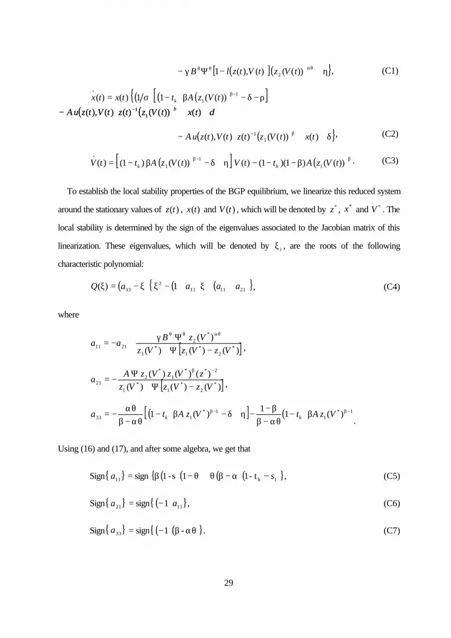
Sign 11 a = sign ( ) ( ) ( ) ( ) 1ht-1 1 s-1 s−α−βθ+θ−β , (C5)

Sign 21 a = sign ( ) 11 1 a− , (C6)

Sign 33 a = sign ( )( ) αθβ− - 1 . (C7)

( ) ( ) δβ ++− − )())(()( )(),( 11 txtVztztVtzuA ( ) ( ) δβ ++− − )())(()( )(),( 11 txtVztztVtzuA

30

At this point, one can easily prove the Proposition 3. First, know that one of the roots of

characteristic polynomial (C4) is equal 33a . Moreover, we observe that the expression inside

brackets in (C4) is not more than the characteristic polynomial associated with the sub-matrix

obtained from dropping the last row and the last column of the Jacobian matrix. The trace and the

determinant of this sub-matrix are equal to ( )111 a+ and ( )2111 aa + , respectively. Noting that the

trace is also given by the sum of its eigenvalues and the determinant by the product of its eigenvalues,

we easily get the sign of the other two roots of the characteristic polynomial (C4). Thus, the result

directly follows.

References.

J. Alonso-Carrera, (1999): "The subsidy to human capital accumulation in a two-sector model ofendogenous growth: A comparative dynamic analysis," mimeo, Universidade de Vigo.

R. Barro and X. Sala-i-Martin, (1995): "Economic growth," McGraw-Hill.

G. Becker, (1965): "A theory of the allocation of time," The Economic Journal LXXV (299): 493-

517.

Benhabib, J., and R. Farmer, (1999): “Indeterminacy and sunspot in macroeconomics,” in

Handbook of Macroeconomics, J. Taylor and M Woodford editors, North Holland,

Amsterdam.

Benhabib, J., and R. Perli (1994). "Uniqueness and Indeterminacy: on the Dynamics of Endogenous

Growth," Journal of Economic Theory 63: 113-142.

E. Bond, P. Wang and C. Yip, (1996): "A general two-sector model of endogenous growth with

human and physical capital: Balanced growth and transitional dynamics," Journal of Economic

Theory, 68: 149-173.

G. Glomm and B. Ravikumar, (1992): "Public versus private investment in human capital:

Endogenous growth and income inequality," Journal of Political Economy 100(4): 818-834.

31

L. Jones, R. Manuelli, P. Rossi, (1997): "On the optimal taxation of capital income," Journal of

Economic Theory 72: 93-117.

R. King, C. Plosser and S. Rebelo, (1988):"Production, growth and business cycles: II. New

Directions," Journal of Monetary Economics 21: 309-41.

R. Lucas, (1988): "On the mechanics of economic development," Journal of Monetary Economics

22: 3-42.

R. Lucas, (1990): "Supply-side Economics: An analytical review," Oxford Economic Papers 42:

293-316.

G. M. Milesi-Ferretti and N. Roubini, (1998a): "On the taxation of human and physical capital in

models of endogenous growth," Journal of Public Economics 70: 237-254.

G. M. Milesi-Ferretti and N. Roubini, (1998b): "Growth effects of income and consumption taxes,"

Journal of Money, Credit and Banking 30(4): 721-744.

K. Mino, (1996) "Analysis of a two-sector model of endogenous growth with capital income

taxation," International Economic Review 37(1): 227-253.

S. Ortigueira, (1998): "Fiscal policy in an endogenous growth model with human capital

accumulation," Journal of Monetary Economics 42: 323-355.

R. Perli and P. Sakellaris, (1998): "Human capital formation and business cycle persistence, "

Journal of Monetary Economics 42: 67-92.

S. Rebelo and N. L. Stokey, (1995): "Growth effects of flat-rate taxes," Journal of Political

Economy 103(3): 519-550.

H. Uzawa, (1964): "Optimal growth in a two-sector model of capital accumulation," Review of

Economic Studies, 31: 1-24.