New approach for proximate analysis by thermogravimetry ...

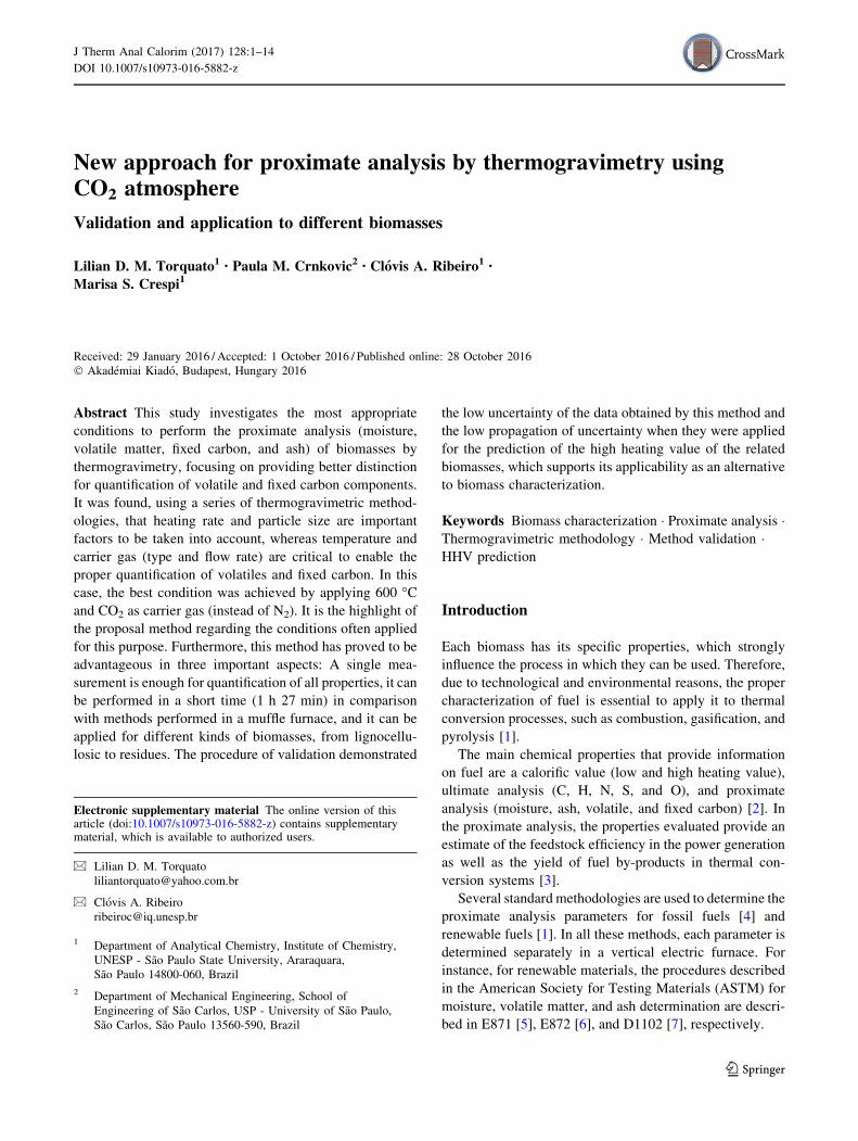
New approach for proximate analysis by thermogravimetry usingCO2 atmosphere

Validation and application to different biomasses

Lilian D. M. Torquato1• Paula M. Crnkovic2

• Clovis A. Ribeiro1•

Marisa S. Crespi1

Received: 29 January 2016 / Accepted: 1 October 2016 / Published online: 28 October 2016

� Akademiai Kiado, Budapest, Hungary 2016

Abstract This study investigates the most appropriate

conditions to perform the proximate analysis (moisture,

volatile matter, fixed carbon, and ash) of biomasses by

thermogravimetry, focusing on providing better distinction

for quantification of volatile and fixed carbon components.

It was found, using a series of thermogravimetric method-

ologies, that heating rate and particle size are important

factors to be taken into account, whereas temperature and

carrier gas (type and flow rate) are critical to enable the

proper quantification of volatiles and fixed carbon. In this

case, the best condition was achieved by applying 600 �Cand CO2 as carrier gas (instead of N2). It is the highlight of

the proposal method regarding the conditions often applied

for this purpose. Furthermore, this method has proved to be

advantageous in three important aspects: A single mea-

surement is enough for quantification of all properties, it can

be performed in a short time (1 h 27 min) in comparison

with methods performed in a muffle furnace, and it can be

applied for different kinds of biomasses, from lignocellu-

losic to residues. The procedure of validation demonstrated

the low uncertainty of the data obtained by this method and

the low propagation of uncertainty when they were applied

for the prediction of the high heating value of the related

biomasses, which supports its applicability as an alternative

to biomass characterization.

Keywords Biomass characterization � Proximate analysis �Thermogravimetric methodology � Method validation �HHV prediction

Introduction

Each biomass has its specific properties, which strongly

influence the process in which they can be used. Therefore,

due to technological and environmental reasons, the proper

characterization of fuel is essential to apply it to thermal

conversion processes, such as combustion, gasification, and

pyrolysis [1].

The main chemical properties that provide information

on fuel are a calorific value (low and high heating value),

ultimate analysis (C, H, N, S, and O), and proximate

analysis (moisture, ash, volatile, and fixed carbon) [2]. In

the proximate analysis, the properties evaluated provide an

estimate of the feedstock efficiency in the power generation

as well as the yield of fuel by-products in thermal con-

version systems [3].

Several standard methodologies are used to determine the

proximate analysis parameters for fossil fuels [4] and

renewable fuels [1]. In all these methods, each parameter is

determined separately in a vertical electric furnace. For

instance, for renewable materials, the procedures described

in the American Society for Testing Materials (ASTM) for

moisture, volatile matter, and ash determination are descri-

bed in E871 [5], E872 [6], and D1102 [7], respectively.

Electronic supplementary material The online version of thisarticle (doi:10.1007/s10973-016-5882-z) contains supplementarymaterial, which is available to authorized users.

& Lilian D. M. Torquato

[email protected]

& Clovis A. Ribeiro

[email protected]

1 Department of Analytical Chemistry, Institute of Chemistry,

UNESP - Sao Paulo State University, Araraquara,

Sao Paulo 14800-060, Brazil

2 Department of Mechanical Engineering, School of

Engineering of Sao Carlos, USP - University of Sao Paulo,

Sao Carlos, Sao Paulo 13560-590, Brazil

123

J Therm Anal Calorim (2017) 128:1–14

DOI 10.1007/s10973-016-5882-z

http://dx.doi.org/10.1007/s10973-016-5882-z

http://crossmark.crossref.org/dialog/?doi=10.1007/s10973-016-5882-z&domain=pdf

http://crossmark.crossref.org/dialog/?doi=10.1007/s10973-016-5882-z&domain=pdf

Fixed carbon is only obtained by mass difference,

which strongly depends on the other parameters deter-

mined previously, so the samples employed in each pro-

cedure must have the same moisture contents [8]. This

requirement can represent a limitation for application of

such methods.

In the case of biomass, it would be reasonable to

adopt the proximate analysis methods developed for

wood fuels (ASTM E872) because of their similar

composition, despite their diversity. Meanwhile, these

methods have previously been developed based on those

for fossil fuels (ASTM D3175) [9], employing very high

temperatures (950 �C), particularly in the case of vola-

tiles determination. However, biomass devolatilization

takes place at a lower temperature, compared to coals

[10], due to the differences in their compositional

structures. When such high temperatures are applied to

biomass materials, the decomposition of the sample can

occur before the evaluation of the fixed carbon content.

Therefore, the analysis of biomass using techniques

originally designed for fossil fuels could result in unre-

liable data.

Also, although these standard methodologies are already

laid down for the performance of proximate analysis, they

are time-consuming and require large amounts of samples.

They also depend on the accuracy of the operator and

comprise several steps, which may result in low

reproducibility.

Thermogravimetry has been described as a suit-

able technique for proximate analysis determination for

both fossil fuels [11–16] and biofuels [17, 18]. It is a

valuable quantitative analytical method because it enables

a continuous and fast measurement under controlled tem-

perature conditions, employs a small sample mass, requires

minimal operator intervention, and is low risk. However, to

achieve these benefits is essential the prior knowledge of

the composition of the sample as well as the influence of

experimental conditions on its characterization by means of

thermal analysis techniques.

Hence, considering the importance of proximate analy-

sis for characterization of biomass for energy use, the goal

of this work was to evaluate the most appropriate condi-

tions for determination of moisture, volatile matter, fixed

carbon, and ash contents in biomass by thermogravimetry.

For this reason, this study evaluates a set of thermogravi-

metric methodologies, considering critical experimental

parameters such as temperature, heating rate, particle size,

as well as type, and flow rate of the carrier gas.

The best conditions were summarized in a thermo-

gravimetric methodology, and the method was then vali-

dated to ensure their applicability and reproducibility to

different types of biomass.

Materials and methods

Biomass samples: source and preparation

Different types of biomass samples were studied: two

samples of sewage sludge from different sources and lig-

nocellulosic agricultural residues. Their chemical proper-

ties are shown in Table 1.

The lignocellulosic samples were pine (Pinus elliottii

engelm) sawdust, peanut (Arachis hypogaea) shell, coffee

(Coffea arabica) husk, rice (Oryza sativa) husk, tucuma

(Astrocaryum aculeatum) seed (endocarp), and sugar cane

(Sacharaum officinarum) bagasse. They were obtained in

different regions of Brazil. Pine sawdust, sugar cane bagasse,

peanut shell, and coffee husk were obtained from industrial

facilities, respectively, in the cities of Itapeva (23�5805600S,

48�5203200W), Ibate (21�5701700S, 47�5904800W), Botucatu

(22�5300900S, 48�2604200W), and Campinas (22�5402100S,

47�303900W), in Sao Paulo State. Rice husk was obtained in

State of Maranhao (02�3101700S, 45�0405700W), and tucuma

seed was collected from the Amazon rainforest, State of

Para.

Regarding to sludge samples, they were generated from the

biological sewage treatment in urban wastewater treatment

plants (UWWTP) of Araraquara (21�4704100S, 48�1003400W)

and Sao Jose do Rio Preto (20�4901300S, 49�2204700W), both

cities of Sao Paulo State, Brazil. In Araraquara, the sewage is

subjected to aeration using full pond mixing, while in Sao

Jose do Rio Preto a mixed treatment system is used (anaerobic

followed by aeration with activated sludge).

All samples were dried at 100 ± 5 �C for 24 h, then

grinded, and manually sieved (A Bronzinox sieves; Sao

Paulo, Brazil). In order to address the contribution of the

particle size to proximate analysis, sieves with different

mesh sizes (Tyler) 500, 250, and 160 lm were employed.

Thus, after being dried and grinded, all samples were

passed through the sieves arranged in sequence. Therefore,

the average granulometry between 500 and 250 lm was

designated as ‘375 lm,’ whereas the average granulometry

between 250 and 160 lm was designated as ‘205 lm.’

The elemental analysis was performed in the EA1110-

CHNS-O elemental analyzer (CE Instruments; Milan,

Italy), and the high heating values (HHV) of samples was

determined in the IKA C 2000 oxygen bomb calorimeter

(IKA Works Inc.; Staufen, Germany).

Thermogravimetric experiments

All the experiments were carried out in the SDT 2960

Simultaneous TGA-DTA thermal analyzer (TA Instru-

ments; New Castle, DE, USA), with the test materials

placed in inert a-alumina sample holder. Before the

2 L. D. M. Torquato et al.

123

experiments, the equipment was calibrated for baseline,

mass (with standard masses), and temperature (from the

melting point of indium) in each experimental condition

evaluated (heating rate, final temperature, and carrier gas).

A series of methods (M1, M2. M3, M4, M5, M5, M6,

M7, and M8) consisting of different stepwise heating

programs were designed to evaluate the influence of tem-

perature, heating rate, and the furnace atmosphere on the

release of volatiles. Table 2 presents the conditions estab-

lished for each method.

The thermogravimetric programming considered two

steps: (1) moisture and volatiles contents; (2) fixed carbon

and ash contents. Step 1 was conducted under nitrogen (N2)

or carbon dioxide (CO2) atmospheres, with gas flow rates

of 130 mL min-1. In each method, the same heating rate

was maintained in both steps.

For moisture content determination, heating at 110 �Cwas employed in all experiments. This temperature is an

average of the values employed in several different standard

methods E1131 [19], D7582 [11], E871 [5], and D3173

[20]. After reaching this temperature, the hold time

(isothermal condition) adopted for the first experiments

(30 min) was reduced to 15 min for the subsequent exper-

iments (M3–M8), since it was enough to ensure the mass

stabilization before the next stage. For volatiles determi-

nation, the first experiments (M1 and M2) employed a final

temperature of 950 �C, based on standard method E872 [6].

Step 2 was performed after switching to an oxidizing

atmosphere (compressed air, at a flow rate of

100 mL min-1). In this step, fixed carbon was determined

from the mass loss caused by the chemical reaction

between oxygen and fixed carbon.

According to the E1131 [19] standard method, the

temperature of 750 �C was employed as the starting point

for quantification of this component after volatiles release

(M1, M2, and M3). However, lower temperatures such as

700 �C (M4), 650 �C (M5), and 600 �C (M6, M7, and M8)

were subsequently evaluated in order to improve the sep-

aration of these components. The final residue represents

the ash content of biomass sample.

The heating rate, particle size as well as type, and flow

rate of the carrier gas were also evaluated. About heating

rate, a comparison between 20 �C min-1 (M6),

30 �C min-1 (M7), and 50 �C min-1 (M8) was made. The

granulometry of particles in the samples tested, as previ-

ously mentioned, ranged from 106 to 500 lm. The carrier

gasses employed were CO2 and N2, at flow rates between

30 and 130 mL min-1. The default sample mass used was

10 mg, which is recommended by E1131 [19] and provided

a satisfactory mass distribution in the sample holder (close

to half of its capacity), ensuring good thermal conductivity.

The main difference between M1 and M2 is that before

fixed carbon evaluation, the release of volatiles content is

performed up to 950 �C, the first one under N2 and the

second, under CO2. The M3, M4, M5, and M6 methods

were performed to evaluate the influence of temperature:

750, 700, 650, and 600 �C, respectively. On the other hand,

the effects of increasing the heating rate may be observed

from M6 to M8. From M3, all methods were performed

under CO2 atmosphere.

All the experimental conditions were assessed for each

biomass type in search of plateau regions (with constant

mass) in the thermogravimetric curves, which are essential

to enable the distinction and quantification of each

parameter in the continuous measurement.

Validation of method

To validate the thermal analytical method (M8), we cal-

culated the confidence interval as well as the propagation

of uncertainty of the data obtained from 10 replicates of

pine sawdust and sewage sludge (from mixed STP). The

Table 1 Chemical properties of biomass samples

Biomass samples HHV/MJ kg-1 Elemental analysis/mass%, dry basis

C H N S O

Sewage sludges

Mixed STPa 13.94 31.73 6.34 4.37 0.78 27.51

Aerobic STPb 12.12 28.12 4.08 3.29 0.90 17.30

Peanut shell 16.52 41.52 7.43 2.11 0.60 27.74

Pine sawdust 17.03 45.95 7.46 0.32 0.60 34.17

Coffee husk 16.79 43.13 5.93 1.55 0.67 32.85

Rice husk 15.39 31.46 6.67 1.04 0.51 22.91

Tucuma seed 20.77 48.83 6.71 0.88 – 32.43

Sugar cane bagasse 17.46 45.05 5.57 0.25 – 38.24

a Sludge from mixed sewage treatment plant (anaerobic ? aerobic)b Sludge from aerobic sewage treatment plant by full pond mixing

New approach for proximate analysis by thermogravimetry using CO2 atmosphere 3

123

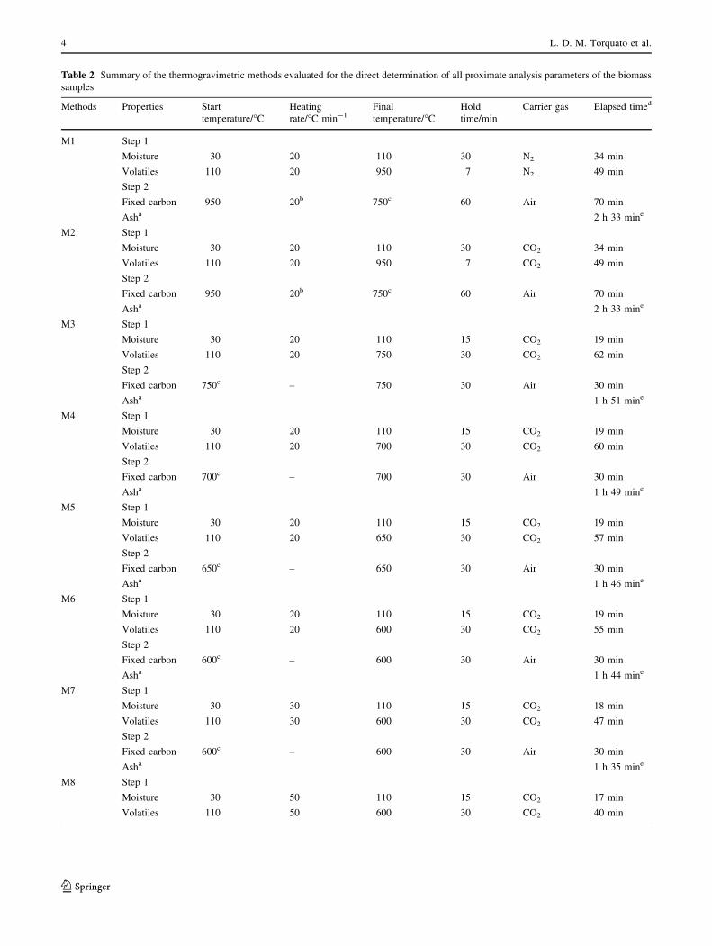
Table 2 Summary of the thermogravimetric methods evaluated for the direct determination of all proximate analysis parameters of the biomass

samples

Methods Properties Start

temperature/�CHeating

rate/�C min-1Final

temperature/�CHold

time/min

Carrier gas Elapsed timed

M1 Step 1

Moisture 30 20 110 30 N2 34 min

Volatiles 110 20 950 7 N2 49 min

Step 2

Fixed carbon 950 20b 750c 60 Air 70 min

Asha 2 h 33 mine

M2 Step 1

Moisture 30 20 110 30 CO2 34 min

Volatiles 110 20 950 7 CO2 49 min

Step 2

Fixed carbon 950 20b 750c 60 Air 70 min

Asha 2 h 33 mine

M3 Step 1



Step 2

Fixed carbon 750c – 750 30 Air 30 min

Asha 1 h 51 mine

M4 Step 1



Step 2


Asha 1 h 49 mine

M5 Step 1



Step 2


Asha 1 h 46 mine

M6 Step 1



Step 2


Asha 1 h 44 mine

M7 Step 1



Step 2


Asha 1 h 35 mine

M8 Step 1




123

measures required for the method validation were per-

formed using the average masses of 10.14 ± 0.11 and

10.15 ± 0.12 mg, respectively.

The confidence interval was estimated for each param-

eter (moisture, volatiles, fixed carbon, and ash) by assum-

ing a 95% confidence level (significance level of 0.05). For

uncertainty estimation, we calculated the uncertainty con-

tribution of each parameter as well as the combined stan-

dard uncertainty, when they were applied to predict the

HHV of the related biomasses, by means of three different

equations: Eqs. 1–3.

HHV MJ kg�1� �

¼ 0:3536 FCð Þ þ 0:1559 VMð Þ� 0:0078 Ashð Þ ð1Þ


¼ 19:2880 � 0:2135VM

FC

� �

þ 0:0234FC

Ash

� �� 1:9584

Ash

VM

� �

ð2Þ

HHV MJkg�1� �

¼ 20:7999 � 0:3214VM

FC

� �

þ 0:0051VM

FC

� �2

� 11:2277Ash

VM

� �

þ 4:4953Ash

VM

� �2

� 0:7223Ash

VM

� �3

þ 0:0383Ash

VM

� �4

þ 0:0076FC

Ash

� �

ð3Þ

where FC is fixed carbon and VM is volatile matter present

in biomass.

The standard uncertainties (SU) resulting from the

application of proximate analysis parameters (from M8) in

the prediction of HHV, according to Eqs. 1–3, are

expressed in Eqs. 4–6, respectively. Note that in the case of

nonlinear Eq. 3, either Eq. 5 or 6 might be used to calcu-

late the standard uncertainty of its terms. All these calcu-

lations were performed according to EURACHEM Guide

[21], using the spreadsheet software Microsoft Excel�,

version 2013.

If u ¼ kx; Dux ¼ kDx ð4Þ

where u is a single term of Eq. 1, k is the constant value, x

is the proximate analysis parameter, Dux is the standard

uncertainty of this term, and Dx is the standard deviation of

the parameter calculated by the mean of values (from the

replicate of experiments).

If u ¼ x=y; ðDuÞ2 ¼ ½1=y2ðDxÞ2 þ� ½x2=y4 DyÞ2� i

ð5Þ

where u is a single term of Eq. 2 or 3, x and y are the prox-

imate analysis parameters, Dx and Dy are the respective

standard deviations, andDu is the standard uncertainty of this

term, expressed as a sum of relative standard deviations.

If u ¼ zn; for z ¼ x=y; Du ¼ n u=zð Þ Dzð Þ ð6Þ

where u is a single term of Eq. 3, z is the quotient of

proximate analysis parameters, n is the power in which z is

raised, Du is the standard uncertainty of the term u, and

Dz is the standard uncertainty of the quotient z, in which

the calculation was demonstrated by Eq. 5.

It is worth noting that after the calculation of the stan-

dard uncertainty according to Eqs. 5 and 6, it is necessary

to multiply each term by its respective constant.

Given the above considerations, the combined standard

uncertainty (CSU) of all components may be expressed as

the positive square root of a sum of the squares of the

individual uncertainty components.

Results and discussion

Volatile and fixed carbon determination

Evaluation of the furnace atmosphere

Figure 1 shows two thermogravimetric curves obtained

using M1 and M2 methods for pine sawdust. For both

Table 2 continued

Methods Properties Start

temperature/�CHeating

rate/�C min-1Final

temperature/�CHold

time/min

Carrier gas Elapsed timed

Step 2


Asha 1 h 27 mine

a Ash content = final residue, calculated by: 100% - [biomass total mass loss (%)]b Cooling rate (�C min-1). This procedure was only applied for M1 and M2c Change point of furnace environmentd Time spent for determination of each parametere Total spent time for determination of all parameters, at the end of step 2


123

methods, the thermal degradation occurs through two steps.

The first, up to 80 min of analysis is related to mass loss of

biomass under N2 (for M1) and CO2 (for M2) atmospheres.

The second, from 80 min up to the end of the analysis

corresponds to the thermal behavior of biomass under air

atmosphere.

The moisture content was successfully determined under

N2 atmosphere, with a plateau obtained after the mass loss

at 110 �C. Subsequently, with an increase in temperature

and during the isothermal step, there was a continuous

mass loss, even before switching to air atmosphere (up to

80 min). This behavior resulted in a TG curve profile in

which it was not possible to distinguish volatile matter and

fixed carbon.

Under N2 atmosphere, the volatile matter content cannot

be determined due to the pyrolysis process that occurs at

higher temperatures (\500 �C). The thermal decomposi-

tion of the main organic components of the biomass gen-

erates oxygenated by-products. As the temperature

gradually increases, these by-products reach their sponta-

neous ignition, and the heat released contributes to the

decomposition of the remaining organic matter. Such

behavior is observed as a continuous mass loss due to the

slight devolatilization [22] up to the end of the heating

programming.

The devolatilization rate of the lignocellulosic biomass

under nitrogen atmosphere depends on the amount of its

components, with the cellulose responsible for the higher

devolatilization rate in the early stage of pyrolysis and the

higher lignin content, resulting in slower devolatilization

with increasing temperature. This behavior was previously

observed and reported by Gani and Naruse [23] in their

study with wood chips.

The second method (M2) involves the replacement of

nitrogen by CO2 and the maintenance of all the other

experimental conditions. The moisture content was suc-

cessfully determined, but this method was unsatisfactory

for the determination of volatile materials.

According to Fig. 1, an event of mass loss occurs prior

to switching from CO2 to air. This behavior can be

explained by the gasification reaction that takes place after

devolatilization. As illustrated in Fig. 2, at lower temper-

atures (\700 �C) less stable compounds are released, and

char is formed by means of the devolatilization process

(reaction 1). In contact with CO2 at higher temperatures

([700 �C), and given sufficient residence time, the char

can undergo a Boudouard reaction, which leads to CO

formation (reaction 2) [24–26].

Biomass ! char þ gases ð1ÞCðcharÞ þ CO2ðgÞ ! 2COðgÞ ð2Þ

The mechanism proposed for the gasification reaction

[27–29] comprises two stages: (i) the adsorption of CO2 in

the active sites of biomass char (C�), leading to the for-

mation of a carbon–oxygen complex (*C(O)), and (ii) CO

release by the rearrangement of *C(O). The oxygen

exchange phenomenon is expressed according to reac-

tion 3. The carbon transfer from the solid phase to the gas

phase (unidirectional reaction) is represented by reaction 4.

COðcharÞ þ CO2ðgÞ ��C Oð ÞðcharÞ þ COðgÞ ð3Þ

�C Oð ÞðcharÞ! COðgÞ þ nCOðcharÞ ð4Þ

According to Ergun [30], the reduction of carbon dioxide to

carbon monoxide on a carbon surface (reaction 3) occurs at

temperatures as low as 600 �C. On the other hand, CO is

also generated from the biomass devolatilization [29].

When the concentration of CO is higher than that of the

thermodynamic equilibrium between CO and CO2, the

00

20

2015 mi

Time/min

n

7 min

M1

M2

N2

CO2

air

40

40

60

60

80

80

100

100

150

300

450

600

Tem

pera

ture

/°C

Vol

atili

zed

mas

s/%

750

900

0

Fig. 1 Comparison between the thermogravimetric profiles for

proximate analysis of pine sawdust (205 lm particle size) performed

up to 950 �C, using nitrogen and carbon dioxide atmospheres

(130 mL min-1)

CO2 atmosphere

Temp. < 700 °C

Temp. > 700 °C

+ ashes

Boudouard reaction

C (char) + CO2 → 2CO

Biomass

Devolatilization

Gasification

char + gases (1)

(2)

Fig. 2 Devolatilization and gasification of biomasses in CO2

atmosphere


123

equilibrium of reaction 3 is shifted to the reagent side,

resulting in a free site and consequently preventing the

occurrence of reaction 4. Hence, at lower temperatures CO

becomes an inhibitor of char gasification [30].

Furthermore, char gasification is thermodynamically

susceptible at temperatures above 720 �C [31], reaching

higher yields between 800 and 950 �C [32].

Therefore, the use of temperatures of up to 950 �C is not

appropriate for the quantification of volatile and fixed

carbon contents, in either N2 or CO2 atmospheres. The

effect of temperature on the determinations was therefore

evaluated using lower temperatures (600, 650, 700, and

750 �C).

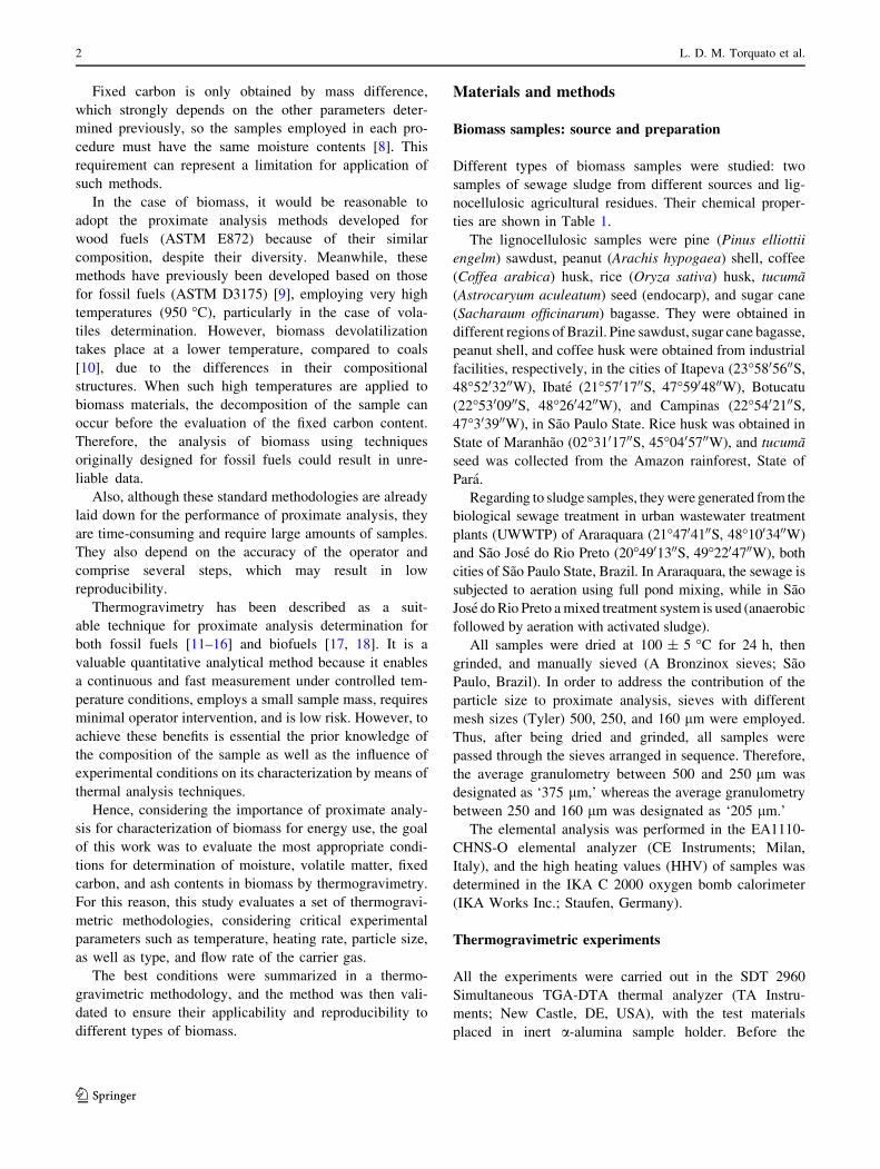
Evaluation of temperature

The main objective of reducing the temperature was to

achieve a mass loss plateau in the TG curves after the

release of the volatile matter to ensure its separation from

the fixed carbon content.

A series of four methods (M3, M4, M5, and M6) were

designed with temperatures of 750, 700, 650, and 600 �C,

respectively, as described in Table 2. The thermogravi-

metric curves obtained for each method are shown in

Fig. 3. Pine sawdust was the sample chosen to illustrate the

TG profile for lignocellulosic biomass.

The temperature was found to have a significant effect

on the volatile matter determination, because as the final

temperature was decreased, there was a trend toward

reaching a plateau in the TG curves up to the end of iso-

therm period in step (1), i.e., before the atmosphere had

been switched from CO2 to air.

As shown in Fig. 3a, when 750 �C was applied as the

final temperature of step (1), there was no evidence of

reaching a plateau in the TG curve. Such behavior indicates

that the fixed carbon present in the sample is decomposed

together with the volatiles. Therefore, under 750 �C, it was

not possible to distinguish or quantify these biomass

fractions.

On the other hand, when 600 �C was applied as the final

temperature of step (1), a trend toward reaching a mass loss

plateau can be observed after the complete devolatilization

and the volatile matter can be quantified. The related TG

curve profile enables the assessment of the fixed carbon

content after the carrier gas has been switched to air and

the complete combustion has occurred.

To ensure that the best choice of the final temperature

would be 600 �C, another type of biomass was evaluated,

the sewage sludge. The TG curves of this residue are

shown in Fig. 3b. The increase in the final temperature

(from 600 to 750 �C) had an even greater effect on the

release of volatile compounds in complex biomasses, such

as sewage sludge. This change in temperature provided TG

profiles with the same value of ash content. Thereby, as the

total mass loss of biomasses did not change, the differences

observed in their TG curves might be due to the increase in

the rate of organic matter decomposition and not due to the

heterogeneity of the samples.

Most studies have shown that both lignocellulosic and

waste biomass materials have their major devolatilization

zone (around 95% of total mass loss) at temperatures of up

to 600 �C [10, 22, 25].

Moreover, clay minerals and carbonates present in large

amounts in biomasses such as sludge and municipal solid

waste decompose at temperatures around 750 �C [33].

Thereby, the application of such high temperatures for the

quantification of volatile organic contents in this type of

biomass may also lead to inappropriate results in proximate

analysis. The temperature of 600 �C is, therefore, the most

suitable to quantify and distinguish volatile and fixed car-

bon in biomass samples.

After the assessment of the most suitable furnace

atmosphere and temperature for the proximate analysis,

Time/min

00

20

20

40

40

60

60

80

M6M3

M6M5M4M3

0 20 40 60 80 1000

150

Tem

pera

ture

/°C

Tem

pera

ture

/°C

Vol

atili

zed

mas

s/%

Vol

atili

zed

mas

s/%

300

450

600

750

0

150

300

450

600

750

airCO2

airCO2

80

100

0

20

40

60

(a)

(b)

80

100

Time/min

Fig. 3 Thermogravimetric curves for: a pine sawdust sample apply-

ing M3, M4, M5, and M6 methods, b sewage sludge sample applying

M3 and M6 methods. Evaluation of the effect of temperature increase

on determination of volatile matter and fixed carbon


123

other experimental conditions were evaluated to improve

the proposed methodology.

Evaluation of the influence of other experimental

conditions

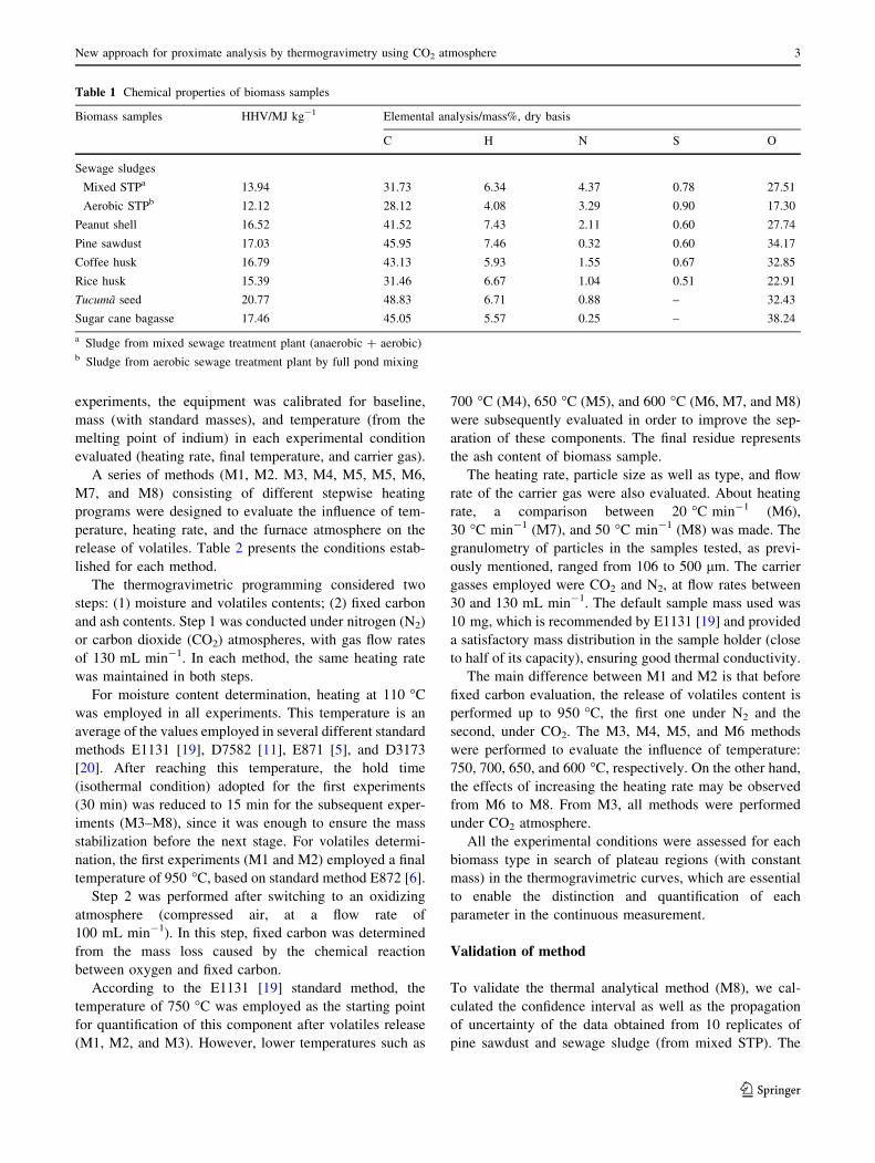
Biomass particle size

TG curves of different particles sizes (\106, 205, 375, and

[500 lm) obtained by the M6 method for lignocellulosic

material and sewage sludge are shown in Fig. 4. The TG

curve profiles for both samples and all particle sizes were

similar with respect to devolatilization and char combus-

tion. However, the behavior of particle sizes\106 lm was

different from the others. In this case, there was a lower

mass loss in devolatilization and a corresponding increase

in the ash content.

These results were unexpected since both volatile matter

and ash contents are characteristics of the samples and

should not depend on the particle size. However, they are

in agreement with those reported by Bridgeman et al. [34],

who evaluated different fractions of crops and observed

that the inorganic constituents are segregated from the

lignocellulosic components during the milling and further

sieving. This process favors the selection and the accu-

mulation of inorganic components, which have smaller

particles, resulting in higher ash and relative lower volatile

matter contents.

This behavior was even more pronounced for sewage

sludge, i.e., the TG curves obtained for smaller particles

(Fig. 4b) showed approximately 10% less mass loss during

the devolatilization, compared to the larger particles,

because this residue contains large amount of inorganic

compounds coming from the wastewater and retained

during the treatment in UWWTP.

Therefore, the particle size is an important parameter

that must be taken into account for the application of the

thermogravimetric method. The results showed that parti-

cles of 205 lm or larger should preferably be used in these

analyses.

Heating rate

The TG curves of the pine sawdust and sewage sludge

samples (205 lm particle size) obtained from room tem-

perature to 600 �C at different heating rates 20 �C min-1

(M6), 30 �C min-1 (M7), and 50 �C min-1 (M8) are

shown in the supplementary data (Fig. S1). It is clear that

for both biomasses, the increase in the heating rate causes a

more pronounced devolatilization, although this did not

affect the attainment of constant mass under isothermal

condition.

According to Lai et al. [25], for a very complex bio-

masses, such as MSW (municipal solid wastes), the

increase in heating rate shortens the devolatilization time

and may increase the residual mass under CO2 atmosphere.

However, in the present case, the results obtained for both

lignocellulosic and sewage sludge samples showed no

increase in residual mass (ash content) when the heating

rate changed from 20 to 50 �C min-1.

These results indicate that the high heating rate of

50 �C min-1 (M8) may be used, without affecting the

quantification of biomass properties, besides allowing the

time saving during proximate analysis.

Type and flow of the carrier gas

Figure 5 shows the TG curves obtained using CO2 as a

carrier gas under three different flow rates (70, 100, and

130 mL min-1) for pine sawdust. The flow rate of

130 mL min-1 was selected because it enables the stabi-

lization of the mass and the volatile matter can be therefore

completely released before the stage of fixed carbon

evaluation.

0 20 40 60 80 100

Time/min

0 20 40 60 80 100

Time/min

0

150858075700

10

20

Tem

pera

ture

/°C

300

450

600

air

< 106 μm

< 106 μm

> 500 μm375 μm205 μm

> 500 μm205 μm

CO2

airCO2

0

150

Tem

pera

ture

/°C

300

450

600

Vol

atili

zed

mas

s/%

0

20

40

60

(a)

(b)

80

100

Vol

atili

zed

mas

s/%

0

20

40

60

80

100

Fig. 4 Thermogravimetric curves obtained by M6 method using

different particle sizes (\106, 205, 375 and [500 lm) of: a pine

sawdust, b sewage sludge


123

Figure 6 shows the TG curves for two different ligno-

cellulosic biomass samples pine sawdust and peanut shell

(Fig. 6a, b, respectively), and sludge (Fig. 6c) under both

N2 and CO2 atmospheres, employing flow rates of

130 mL min-1. The results evidence that when N2 is used,

it was not possible to identify the devolatilization endpoint

after the isothermal period. On the other hand, the use of

CO2 greatly improved the achievement of a mass loss

plateau during the isothermal step, enabling the discrimi-

nation and quantification of the contents of volatile mate-

rial and fixed carbon in the biomass samples.

According to Borrego and Alvarez [35], the use of CO2

as a carrier gas provided higher resistance to the

devolatilization of bulk components of wood chips about

N2. It may be due to the involvement of CO2 in the ‘cross-

linking’ reaction on the surface of the char, which reduces

the deformation and clumping of the carbonaceous struc-

ture. However, morphological characteristics, as well as the

reactivity of char surface, are similar under both atmo-

spheres [24, 36].

After the evaluation of several parameters for the

methodology optimization, it was clear that CO2, instead of

N2, is more suitable for reaching a mass loss plateau after

biomass devolatilization.

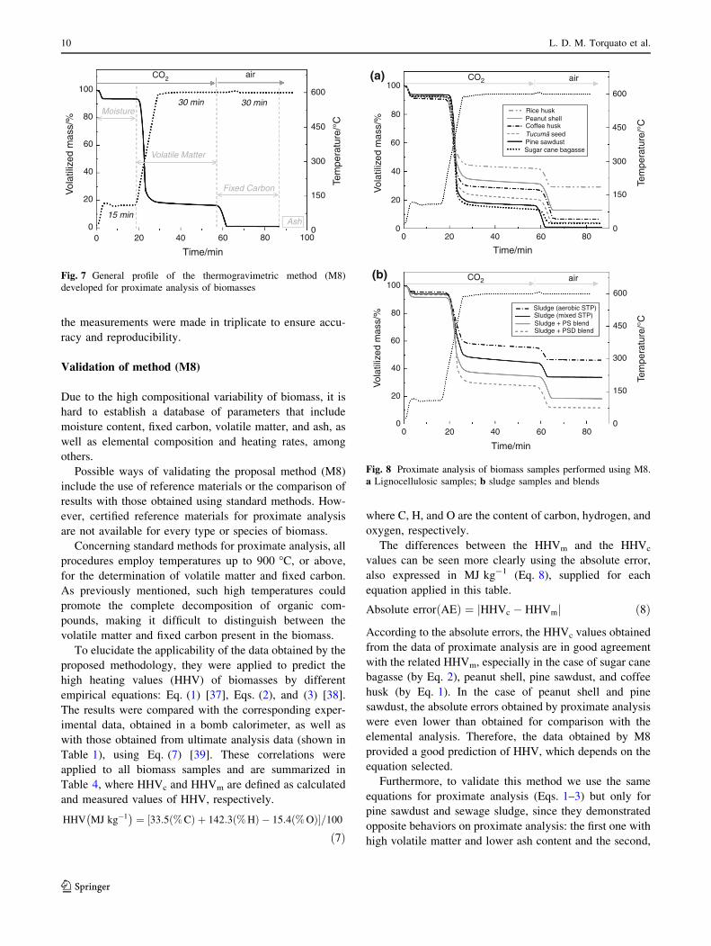
Summary of findings and application to samples

Figure 7 provides an overview of the TG curve obtained

using the optimized conditions for proximate analysis of

the pine sawdust biomass, using the experimental condi-

tions described for M8 method (Table 2). The important

point is that this methodology enables the quantification of

moisture, volatile matter, fixed carbon, and ash in a sig-

nificantly short time (1 h 27 min), compared to the stan-

dard methods.

This methodology was applied in the proximate analysis

of different biomasses (lignocellulosic materials, sewage

sludges, and blends), providing thermogravimetric profiles

specific for each sample type (Fig. 8a, b respectively),

which clearly demonstrate the compositional differences

between them. The data obtained from theses TG curves

are displayed in Table 3. It is worth emphasizing that all

Time/min

0 20 40 60 800

150

Tem

pera

ture

/°C

300

450

600

Vol

atili

zed

mas

s/%

0

20

40

60

80

100air

Heating programming

70 mL min–1

100 mL min–1

130 mL min–1

CO2

Fig. 5 Thermogravimetric profiles for proximate analysis of pine

sawdust, applying M8 method with different flows of carbon dioxide:

70, 100, and 130 mL min-1

Time/min

0 20 40 60 80

Time/min

0 20 40 60 80

Time/min

0 20 40 60 80

0

20

40

60

Vol

atili

zed

mas

s/%

80

100

0

20

40

60

Vol

atili

zed

mas

s/%

80

100

0

20

40

60

Vol

atili

zed

mas

s/%

80

100

0

150

Tem

pera

ture

/°C

300

450

600

0

150

Tem

pera

ture

/°C

300

450

600

0

150

Tem

pera

ture

/°C

300

450

600

(a)

(b)

(c)

Heating programming

CO2 or N2 air

CO2 or N2 air

CO2 or N2 air

CO2 atmosphere

N2 atmosphere

CO2 atmosphere

N2 atmosphere

CO2 atmosphere

N2 atmosphere

Fig. 6 Comparison between the thermogravimetric profiles of a pine

sawdust, b peanut shell, and c sewage sludge samples, using M8

method under carbon dioxide and nitrogen, both in the flow of

130 mL min-1


123

the measurements were made in triplicate to ensure accu-

racy and reproducibility.

Validation of method (M8)

Due to the high compositional variability of biomass, it is

hard to establish a database of parameters that include

moisture content, fixed carbon, volatile matter, and ash, as

well as elemental composition and heating rates, among

others.

Possible ways of validating the proposal method (M8)

include the use of reference materials or the comparison of

results with those obtained using standard methods. How-

ever, certified reference materials for proximate analysis

are not available for every type or species of biomass.

Concerning standard methods for proximate analysis, all

procedures employ temperatures up to 900 �C, or above,

for the determination of volatile matter and fixed carbon.

As previously mentioned, such high temperatures could

promote the complete decomposition of organic com-

pounds, making it difficult to distinguish between the

volatile matter and fixed carbon present in the biomass.

To elucidate the applicability of the data obtained by the

proposed methodology, they were applied to predict the

high heating values (HHV) of biomasses by different

empirical equations: Eq. (1) [37], Eqs. (2), and (3) [38].

The results were compared with the corresponding exper-

imental data, obtained in a bomb calorimeter, as well as

with those obtained from ultimate analysis data (shown in

Table 1), using Eq. (7) [39]. These correlations were

applied to all biomass samples and are summarized in

Table 4, where HHVc and HHVm are defined as calculated

and measured values of HHV, respectively.


¼ 33:5 %Cð Þ þ 142:3 %Hð Þ � 15:4 %Oð Þ½ �=100

ð7Þ

where C, H, and O are the content of carbon, hydrogen, and

oxygen, respectively.

The differences between the HHVm and the HHVc

values can be seen more clearly using the absolute error,

also expressed in MJ kg-1 (Eq. 8), supplied for each

equation applied in this table.

Absolute error AEð Þ ¼ HHVc � HHVmj j ð8Þ

According to the absolute errors, the HHVc values obtained

from the data of proximate analysis are in good agreement

with the related HHVm, especially in the case of sugar cane

bagasse (by Eq. 2), peanut shell, pine sawdust, and coffee

husk (by Eq. 1). In the case of peanut shell and pine

sawdust, the absolute errors obtained by proximate analysis

were even lower than obtained for comparison with the

elemental analysis. Therefore, the data obtained by M8

provided a good prediction of HHV, which depends on the

equation selected.

Furthermore, to validate this method we use the same

equations for proximate analysis (Eqs. 1–3) but only for

pine sawdust and sewage sludge, since they demonstrated

opposite behaviors on proximate analysis: the first one with

high volatile matter and lower ash content and the second,

0 20 40 60 80 100

Time/min

0

150

Tem

pera

ture

/°C

300

450

600

Vol

atili

zed

mas

s/%

015 min

30 min

CO2

30 min

air

Fixed Carbon

Ash

Volatile Matter

Moisture

20

40

60

80

100

Fig. 7 General profile of the thermogravimetric method (M8)

developed for proximate analysis of biomasses

Time/min

0 20 40 60 80

Time/min

0 20 40 60 80

Tem

pera

ture

/°C

0

150

300

450

Rice huskPeanut shellCoffee huskTucumã seedPine sawdust

Sludge (aerobic STP)Sludge (mixed STP)Sludge + PS blendSludge + PSD blend

Sugar cane bagasse

600

Tem

pera

ture

/°C

0

150

300

450

600

0

20

40

60

Vol

atili

zed

mas

s/% 80

100

0

20

40

60

Vol

atili

zed

mas

s/% 80

100(a)

(b) airCO2

airCO2

Fig. 8 Proximate analysis of biomass samples performed using M8.

a Lignocellulosic samples; b sludge samples and blends


123

with low volatile matter and high ash content. Thus, it

would be possible to observe the propagation of uncer-

tainty for very different biomasses, covering the compo-

sitional range between them.

The confidence interval for all data obtained from

proximate analysis of pine sawdust and sewage sludge

(M8) is shown in Table 5. The values of each property

measured by this methodology are in the range specified

with 95% of confidence.

The width of the confidence interval is the difference

between the upper and the lower limit of the confidence

interval and expresses the uncertainty in measurement. In

other words, the width of a confidence interval is a

parameter that characterizes the dispersion of the values

that could be attributed to the value measured [21].

The higher width of the confidence interval observed for

pine sawdust was in ashes, while to sewage sludge, the

higher width was found in volatiles. For pine sample, it can

be attributed to its very low amount of ashes, sometimes

close to the equipment uncertainty. About the sludge, this

behavior of volatiles is acceptable, given its complex and

heterogeneous organic composition.

With the purpose of demonstrating the effect of this

variance in the prediction of HHV, we calculated the HHV

for Eqs. 1–3, supposing two situations: one of them with all

parameters in the lower limit and the other with an upper

limit of the confidence interval. The oscillation of values of

HHV in this interval can be observed in Table 5.

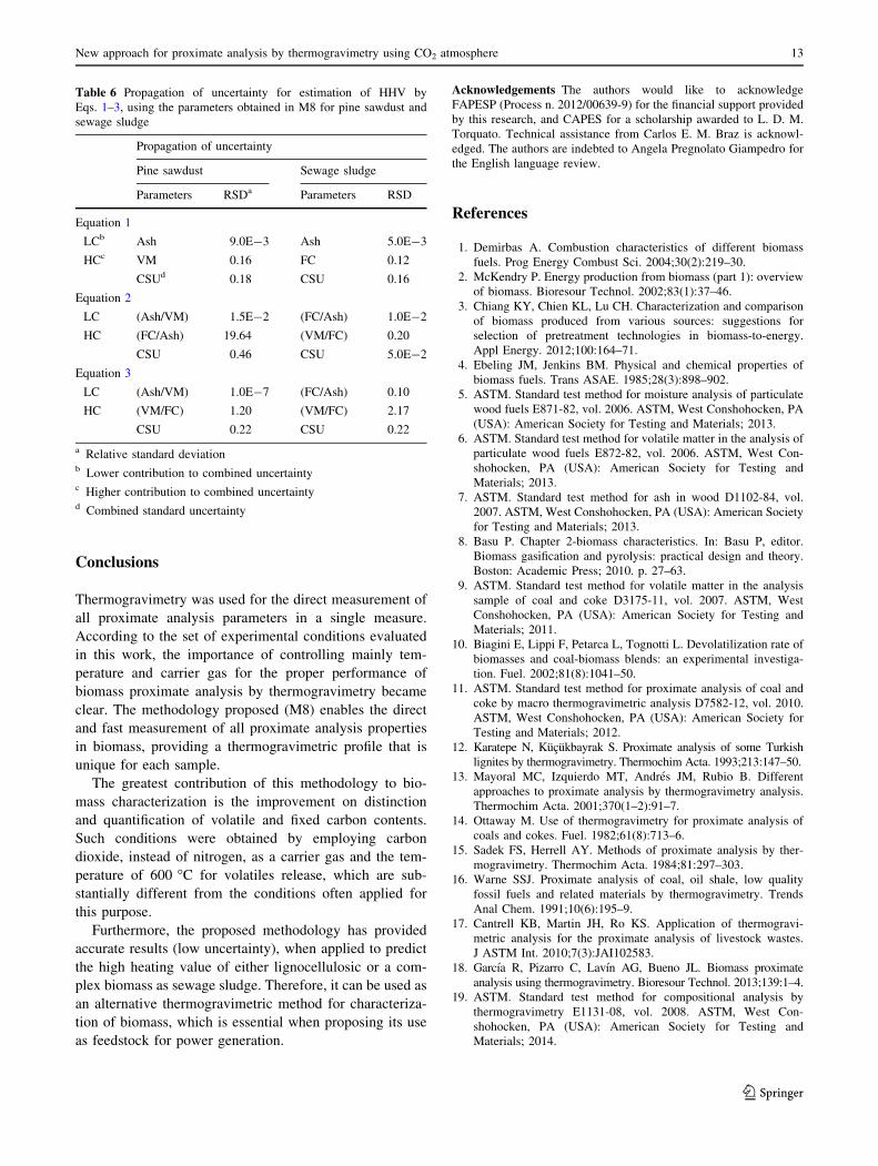
In Table 6 are presented the proximate analysis

parameters (or quotient of parameters) with lower and

higher contribution to the uncertainty calculation as well as

the combined standard uncertainty in the evaluation of

HHV using Eqs. 1–3.

About pine sawdust, the higher source of uncertainty

was the quotient (FC/Ash) in Eq. 2, which reflects in its

higher combined standard uncertainty of 0.46. Concerning

the sludge, the higher contribution to uncertainty estima-

tion was obtained from the term (VM/FC)2, responsible for

the higher combined standard uncertainty of 0.22 for HHV

calculation by Eq. 3.

In general, either pine sawdust or sewage sludge

demonstrated low propagation of uncertainty in the pre-

diction of HHV for all evaluated equations.

The results demonstrated that the data of proximate

analysis obtained with the proposed methodology provided

a good prediction of HHV. In other words, these correla-

tions support the applicability of the data achieved in the

present study by the experimental conditions adopted and

for the range of biomass explored.

Table 3 Properties of proximate analysis obtained for different types

of biomass and blends, using the proposed method (M8)

Biomass samples Proximate analysis/%

Moisture Volatile

matter

Fixed

carbon

Ash

Sewage sludges

Mixed STP 5.25 49.67 9.42 35.66

Aerobic STP 4.70 40.20 8.90 46.30

Peanut shell (PS) 7.43 60.51 18.90 13.17

Pine sawdust (PSD) 6.42 77.68 14.95 0.93

Sludgea ? PS blend 8.43 57.02 16.03 18.51

Sludgeb ? PSD blend 6.74 65.33 16.10 11.83

Coffee husk 9.44 63.15 20.99 6.43

Rice husk 8.14 49.74 12.85 29.27

Tucuma seed 7.27 72.31 16.54 3.88

Sugar cane bagasse 7.39 79.30 9.81 3.50

a Blend composed of 50% sludge from mixed STP ? 50% peanut

shell sampleb Blend composed of 50% sludge from mixed STP ? 50% pine

sawdust sample

Table 4 Comparison between HHVm and HHVc values obtained from proximate and ultimate analysis of biomass samples

Biomass samples HHVm/MJ kg-1 HHVc/MJ kg-1

Proximate analysis Ultimate analysis

Equation (1) AEa Equation (2) AE Equation (3) AE Equation (7) AE

Sewage sludge

Mixed STP 13.94 10.79 3.15 16.76 2.82 13.25 0.69 15.35 1.41

Aerobic STP 12.12 9.05 3.07 16.07 3.95 11.45 0.67 12.57 0.45

Peanut shell 16.52 16.00 0.52 18.21 1.69 17.59 1.07 20.17 3.65

Pine sawdust 17.03 17.38 0.35 18.53 1.50 19.25 2.22 20.83 3.80

Coffee husk 16.79 17.20 0.41 18.52 1.73 18.81 2.02 17.92 1.13

Rice husk 15.39 12.06 3.33 17.32 1.23 14.44 0.95 16.54 1.15

Tucuma seed 20.77 17.08 3.69 18.35 2.42 18.93 1.83 20.95 0.19

Sugar cane bagasse 17.46 15.79 1.66 17.54 0.08 18.07 0.61 17.16 0.30

a Absolute error


123

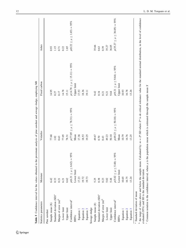
Ta

ble

5C

on

fid

ence

inte

rval

for

the

val

ues

ob

tain

edin

the

pro

xim

ate

anal

ysi

so

fp

ine

saw

du

stan

dse

wag

esl

ud

ge,

emp

loy

ing

M8

Sta

tist

ics

par

amet

ers

Mo

istu

reV

ola

tile

sF

ixed

carb

on

Ash

es

Pin

esa

wd

ust

Sam

ple

mea

n(X

)6

.42

77

.68

14

.95

0.9

3

Sta

nd

ard

dev

iati

on

(SD

)a0

.33

1.0

20

.27

1.1

5

Mar

gin

of

erro

r(m

)b0

.21

0.6

30

.17

0.7

1

Lo

wer

lim

it6

.21

77

.05

14

.78

0.2

2

Up

per

lim

it6

.62

78

.31

15

.11

1.6

5

Co

nfi

den

cein

terv

alc

p(6

.21B

lB

6.6

2)=

95

%p(7

7.0

5B

lB

78

.31

)=

95

%p(1

4.7

8B

lB

15

.11

)=

95

%p

(0.2

2B

lB

1.6

5)=

95

%

HH

Vc

Lo

wer

lim

itM

ean

Up

per

lim

it

Eq

uat

ion

11

7.2

31

7.3

81

7.5

3

Eq

uat

ion

21

9.7

21

8.5

31

8.3

6

Eq

uat

ion

31

9.7

31

9.2

51

9.1

1

Sew

age

slu

dg

e

Sam

ple

mea

n(X

)5

.25

49

.67

9.4

23

5.6

6

Sta

nd

ard

dev

iati

on

(SD

)a0

.38

0.7

00

.34

0.6

3

Mar

gin

of

erro

r(m

)b0

.23

0.4

30

.21

0.3

9

Lo

wer

lim

it5

.02

49

.23

9.2

13

5.2

7

Up

per

lim

it5

.48

50

.10

9.6

43

6.0

5

Co

nfi

den

cein

terv

alc

p(5

.02B

lB

5.4

8)=

95

%p(4

9.2

3B

lB

50

.10

)=

95

%p(9

.21B

lB

9.6

4)=

95

%p

(35

.27B

lB

36

.05

)=

95

%

HH

Vc

Lo

wer

lim

itM

ean

Up

per

lim

it

Eq

uat

ion

11

0.6

51

0.7

91

0.9

3

Eq

uat

ion

21

6.7

51

6.7

61

6.7

8

Eq

uat

ion

31

3.2

41

3.2

51

3.2

6

aS

tan

dar

dd

evia

tio

no

fm

ean

bth

era

ng

eo

fv

alu

esab

ov

ean

db

elo

wth

esa

mp

lem

ean

.C

alcu

late

db

y:

m=

Z*

.SD

wh

ere

Z*

isd

ecr

itic

alto

lera

nce

val

ue

for

the

stan

dar

dn

orm

ald

istr

ibu

tio

n,

inth

ele

vel

of

con

fid

ence

eval

uat

ed(9

5%

)an

dS

Dis

the

stan

dar

dd

evia

tio

nc

Co

mm

on

no

tati

on

toth

eco

nfi

den

cein

terv

al,

wh

erel

isth

ep

op

ula

tio

nm

ean

wh

ich

ises

tim

ated

thro

ug

hth

esa

mp

lem

ean

X


123

Conclusions

Thermogravimetry was used for the direct measurement of

all proximate analysis parameters in a single measure.

According to the set of experimental conditions evaluated

in this work, the importance of controlling mainly tem-

perature and carrier gas for the proper performance of

biomass proximate analysis by thermogravimetry became

clear. The methodology proposed (M8) enables the direct

and fast measurement of all proximate analysis properties

in biomass, providing a thermogravimetric profile that is

unique for each sample.

The greatest contribution of this methodology to bio-

mass characterization is the improvement on distinction

and quantification of volatile and fixed carbon contents.

Such conditions were obtained by employing carbon

dioxide, instead of nitrogen, as a carrier gas and the tem-

perature of 600 �C for volatiles release, which are sub-

stantially different from the conditions often applied for

this purpose.

Furthermore, the proposed methodology has provided

accurate results (low uncertainty), when applied to predict

the high heating value of either lignocellulosic or a com-

plex biomass as sewage sludge. Therefore, it can be used as

an alternative thermogravimetric method for characteriza-

tion of biomass, which is essential when proposing its use

as feedstock for power generation.

Acknowledgements The authors would like to acknowledge

FAPESP (Process n. 2012/00639-9) for the financial support provided

by this research, and CAPES for a scholarship awarded to L. D. M.

Torquato. Technical assistance from Carlos E. M. Braz is acknowl-

edged. The authors are indebted to Angela Pregnolato Giampedro for

the English language review.

References

1. Demirbas A. Combustion characteristics of different biomass

fuels. Prog Energy Combust Sci. 2004;30(2):219–30.

2. McKendry P. Energy production from biomass (part 1): overview

of biomass. Bioresour Technol. 2002;83(1):37–46.

3. Chiang KY, Chien KL, Lu CH. Characterization and comparison

of biomass produced from various sources: suggestions for

selection of pretreatment technologies in biomass-to-energy.

Appl Energy. 2012;100:164–71.

4. Ebeling JM, Jenkins BM. Physical and chemical properties of

biomass fuels. Trans ASAE. 1985;28(3):898–902.

5. ASTM. Standard test method for moisture analysis of particulate

wood fuels E871-82, vol. 2006. ASTM, West Conshohocken, PA

(USA): American Society for Testing and Materials; 2013.

6. ASTM. Standard test method for volatile matter in the analysis of

particulate wood fuels E872-82, vol. 2006. ASTM, West Con-

shohocken, PA (USA): American Society for Testing and

Materials; 2013.

7. ASTM. Standard test method for ash in wood D1102-84, vol.

2007. ASTM, West Conshohocken, PA (USA): American Society

for Testing and Materials; 2013.

8. Basu P. Chapter 2-biomass characteristics. In: Basu P, editor.

Biomass gasification and pyrolysis: practical design and theory.

Boston: Academic Press; 2010. p. 27–63.

9. ASTM. Standard test method for volatile matter in the analysis

sample of coal and coke D3175-11, vol. 2007. ASTM, West

Conshohocken, PA (USA): American Society for Testing and

Materials; 2011.

10. Biagini E, Lippi F, Petarca L, Tognotti L. Devolatilization rate of

biomasses and coal-biomass blends: an experimental investiga-

tion. Fuel. 2002;81(8):1041–50.

11. ASTM. Standard test method for proximate analysis of coal and

coke by macro thermogravimetric analysis D7582-12, vol. 2010.

ASTM, West Conshohocken, PA (USA): American Society for

Testing and Materials; 2012.

12. Karatepe N, Kucukbayrak S. Proximate analysis of some Turkish

lignites by thermogravimetry. Thermochim Acta. 1993;213:147–50.

13. Mayoral MC, Izquierdo MT, Andres JM, Rubio B. Different

approaches to proximate analysis by thermogravimetry analysis.

Thermochim Acta. 2001;370(1–2):91–7.

14. Ottaway M. Use of thermogravimetry for proximate analysis of

coals and cokes. Fuel. 1982;61(8):713–6.

15. Sadek FS, Herrell AY. Methods of proximate analysis by ther-

mogravimetry. Thermochim Acta. 1984;81:297–303.

16. Warne SSJ. Proximate analysis of coal, oil shale, low quality

fossil fuels and related materials by thermogravimetry. Trends

Anal Chem. 1991;10(6):195–9.

17. Cantrell KB, Martin JH, Ro KS. Application of thermogravi-

metric analysis for the proximate analysis of livestock wastes.

J ASTM Int. 2010;7(3):JAI102583.

18. Garcıa R, Pizarro C, Lavın AG, Bueno JL. Biomass proximate

analysis using thermogravimetry. Bioresour Technol. 2013;139:1–4.

19. ASTM. Standard test method for compositional analysis by

thermogravimetry E1131-08, vol. 2008. ASTM, West Con-


Materials; 2014.

Table 6 Propagation of uncertainty for estimation of HHV by

Eqs. 1–3, using the parameters obtained in M8 for pine sawdust and

sewage sludge

Propagation of uncertainty

Pine sawdust Sewage sludge

Parameters RSDa Parameters RSD

Equation 1

LCb Ash 9.0E-3 Ash 5.0E-3

HCc VM 0.16 FC 0.12

CSUd 0.18 CSU 0.16

Equation 2

LC (Ash/VM) 1.5E-2 (FC/Ash) 1.0E-2

HC (FC/Ash) 19.64 (VM/FC) 0.20

CSU 0.46 CSU 5.0E-2

Equation 3

LC (Ash/VM) 1.0E-7 (FC/Ash) 0.10

HC (VM/FC) 1.20 (VM/FC) 2.17

CSU 0.22 CSU 0.22

a Relative standard deviationb Lower contribution to combined uncertaintyc Higher contribution to combined uncertaintyd Combined standard uncertainty


123

20. ASTM. Standard test method for moisture in the analysis sample

of coal and coke D3173-11, vol. 2008. ASTM, West Con-


Materials; 2011.

21. Ellison SLR, Williams A (editors). Eurachem/CITAC guide:

Quantifying Uncertainty in Analytical Measurement, 3rd ed.,

(2012) ISBN 978-0-948926-30-3. Available from www.eur

achem.org.

22. Munir S, Daood SS, Nimmo W, Cunliffe AM, Gibbs BM.

Thermal analysis and devolatilization kinetics of cotton stalk,

sugar cane bagasse and shea meal under nitrogen and air atmo-

spheres. Bioresour Technol. 2009;100(3):1413–8.

23. Gani A, Naruse I. Effect of cellulose and lignin content on

pyrolysis and combustion characteristics for several types of

biomass. Renew Energy. 2007;32(4):649–61.

24. Gil MV, Riaza J, Alvarez L, Pevida C, Pis JJ, Rubiera F. Kinetic

models for the oxy-fuel combustion of coal and coal/biomass

blend chars obtained in N2 and CO2 atmospheres. Energy.

2012;48(1):510–8.

25. Lai Z, Ma X, Tang Y, Lin H. Thermogravimetric analysis of the

thermal decomposition of MSW in N2, CO2, and CO2/N2 atmo-

spheres. Fuel Process Technol. 2012;102:18–23.

26. Moon J, Lee J, Lee U, Hwang J. Transient behavior of

devolatilization and char reaction during steam gasification of

biomass. Bioresour Technol. 2013;133:429–36.

27. Di Blasi C. Combustion and gasification rates of lignocellulosic

chars. Prog Energy Combust Sci. 2009;35(2):121–40.

28. Scott SA, Davidson JF, Dennis JS, Fennell PS, Hayhurst AN. The

rate of gasification by CO2 of chars from waste. Proc Combust

Inst. 2005;30(2):2151–9.

29. Shen D, Hu J, Xiao R, Zhang H, Li S, Gu S. Online evolved gas

analysis by thermogravimetric-mass spectroscopy for thermal

decomposition of biomass and its components under different

atmospheres: part I. Lignin Bioresour Technol. 2013;130:449–56.

30. Ergun S. Kinetics of the reaction of carbon with carbon dioxide.

J Phys Chem. 1956;60(4):480–5.

31. Kwon EE, Jeon YJ, Yi H. New candidate for biofuel feedstock

beyond terrestrial biomass for thermo-chemical process (pyroly-

sis/gasification) enhanced by carbon dioxide (CO2). Bioresour

Technol. 2012;123:673–7.

32. Vamvuka D, Karouki E, Sfakiotakis S. Gasification of waste

biomass chars by carbon dioxide via thermogravimetry. Part I:

effect of mineral matter. Fuel. 2011;90(3):1120–7.

33. Campana A, Martins Q, Crespi M, Ribeiro C, Barud H. Thermal

behavior of residues (sludge) originated from Araraquara water

and sewage treatment station. J Therm Anal Calorim.

2009;97(2):601–4.

34. Bridgeman TG, Darvell LI, Jones JM, Williams PT, Fahmi R,

Bridgwater AV, et al. Influence of particle size on the analytical and

chemical properties of two energy crops. Fuel. 2007;86(1–2):60–72.

35. Borrego AG, Alvarez D. Comparison of chars obtained under

oxy-fuel and conventional pulverized coal combustion atmo-

spheres. Energy Fuels. 2007;21(6):3171–9.

36. Borrego AG, Garavaglia L, Kalkreuth WD. Characteristics of

high heating rate biomass chars prepared under N2 and CO2

atmospheres. Int J Coal Geol. 2009;77(3–4):409–15.

37. Parikh J, Channiwala S, Ghosal G. A correlation for calculating

HHV from proximate analysis of solid fuels. Fuel.

2005;84(5):487–94.

38. Nhuchhen DR, Abdul Salam P. Estimation of higher heating

value of biomass from proximate analysis: a new approach. Fuel.

2012;99:55–63.

39. Nanda S, Mohanty P, Pant KK, Naik S, Kozinski JA, Dalai AK.

Characterization of North American lignocellulosic biomass and

biochars in terms of their candidacy for alternate renewable fuels.

Bioenergy Res. 2012;6(2):663–77.


123

http://www.eurachem.org

http://www.eurachem.org

New approach for proximate analysis by thermogravimetry ...

Documents

Transcript of New approach for proximate analysis by thermogravimetry ...