1

A NEW APPROACH TO UTILITY FUNCTION

Catalin Angelo IOAN

Danubius University, 800654-Galati, Romania

E-mail: catalin_angelo_ioan@univ-danubius.ro

Gina IOAN

Danubius University, 800654-Galati, Romania

E-mail: ginaioan@univ-danubius.ro

Abstract

This paper treats from an axiomatic point of view the notions of indifference and preference,

relative to the consumption of goods. The concept of marginal utility is presented in both

differentiable and, especially, in the discretized case. There are introduced new types of discretized

marginal utility that adapts better when analyzing discrete the differential situation. The marginal rate

of substitution is addressed globally, for n goods, obtaining the notions of hyperplane or minimal

vector of substitution. Also, in the discretized case, there are introduced the marginal rates of

substitution to the left, right, bilateral, as well as the adjusted rates.

Keywords indifference, preference, utility, marginal rate of substitution

Classification codes and keywords: D01

1. INTRODUCTION

From moments of impasse that has passed mathematics at the end of the nineteenth century,

when it was forced relocation and reconstruction of the foundations of rigorous, any scientific theory

that any aims to be sustainable and, above all, rigorous, has a urge to be built on solid bases,

axiomatized.

This field theory make a distance from the field of speculations or circumstantial situations,

giving durability and at the same time, rigorous scientific reasoning.

Any economic activity involves the existence of two distinct entities, but complementary,

namely at least one manufacturer and a single consumer.

A manufacturer can not operate without a specific guarantee the possibility of purchase of his

goods by at least one buyer as such it can not exist an applicant without the real creator of the product

to be asked.

It is natural to assume that each of the two parties follows a well-defined purpose. A

manufacturer which would not pursue its profit maximization (even if this approach is somewhat

simplistic) were closer to a charitable institution, rather than an economic entity. On the other hand, a

beneficiary (which departs net from the notion of consumer) that would purchase products without

having to follow a specific purpose (food needs, comfort, travel, etc.) could easily turn into a collector

therefore, it would affect another individual needs.

It is very difficult to be measured or quantified the consumer’s “need”. A concept, largely

controversial, satisfying to some extent, provided the “primary concept” in any axiomatic theory, is

the utility.

There are a number of theories that define, more or less axiomatic notion of utility directly

related to consumer preference for certain combinations of assets. What is a consumer preference but a

good over another? The answer can only return to the same concept just try to explain it. We will not

deviate too much from this line (even it is questionable from many points of view), but we will try a

systematic and consistent increase in scientific endeavor.

2

2. CONSUMER PREFERENCES

Before defining the consumer space, we consider first, that all goods for consumption are

indefinitely divisible. We will see, a little later, that this convention is to a point, benefit, meaning that

differential techniques can be applied in the analysis of consumer behavior. On the other hand, the

findings obtained will be applied with great caution, especially when we want to establish a consumer

verdict.

We thus define the consumer space on Rn for n fixed assets as SC={(x1,...,xn)xi≥0, i= n,1 }

where x∈SC, x=(x1,...,xn) is a consumption basket or basket of goods.

In relation to the issues raised above, is a natural question: considering two elements x,y∈SC,

how do we characterize that a consumer will choose the basket x or y? It seems then that will have to

establish a certain choice between a basket or another. In order not to enter the above vicious circle,

we define the so-called preference relations, external in the generation of the rigorous theory, but

effective in implementation.

We will define the relationship of indifference on SC noted, in what follows, with: ∼. If two

baskets x and y are in relation x∼y, this means that any combination of goods x and y is indifferent for

the consumer. Also, we note that x ~/ y the fact that x is not indifferent to y.

We will impose the condition of indifference to be a relationship of equivalence that is:

I.1. ∀x∈SC⇒x∼x (reflexivity);

I.2. ∀x,y∈SC, x∼y⇒y∼x (symmetry);

I.3. ∀x,y,z∈SC, x∼y, y∼z⇒x∼z (transitivity).

The interpretation of these axioms is natural. Thus, reflexivity is not merely say that a basket

of goods is indifferent in his choice himself, and symmetry that indifference between x and y implies

choice, inevitably, the indifference of y and x. Transitivity is not always obvious, in that there may be

situations (more or less forced) the indifference between x and y, then y and z between not involve the

binding of x and z. Usually, the deviation from transitivity can occur when the relation of indifference

is not “perfect”, small differences between the three baskets leading to a significant distance between

the extremes.

Let therefore the consumer space endowed with the relationship of indifference defined upper

(SC,∼) and x∈SC. The equivalence class of x: [x]={y∈SCy∼x} will consist in all consumer’s baskets

indifferent respected to x. We will call [x] – the indifference class of x.

From the properties of equivalence classes follow some remarkable conclusions, namely:

• x and y are indifferent if and only if they have identical indifference classes;

• for any two baskets of goods x and y, their indifference classes are either identical or disjoint (i.e.

if exists z such that x∼z, but y ~/ z then for any u∼x will result that u ~/ y;

• the set of all baskets of goods or, in other words, the consumer space is the union of all classes of

consumer indifference.

A system of representatives for the relationship of indifference ∼ will consist of all consumer

baskets such that any two such entities are not indifferent and any consumer basket are whatever

exactly one of the elected representatives.

Before continuing, let recall that a norm on the linear space Rn is an application: ⋅ :R

n→R,

x→ x ∀x∈Rn such that the following axioms are satisfied:

N.1. x =0⇒x=0;

N.2. xα = x⋅α ∀x∈Rn ∀α∈R;

N.3. yxyx +≤+ ∀x,y∈Rn.

The pair (Rn, ⋅ ) is called the normed n-dimensional linear space.

Considering therefore an arbitrary norm ⋅ on Rn we will add a first additional axiom to the

relationship of indifference named the axiom of continuity:

I.4. ∀x,y∈SC, x∼y, x < y ⇒∃z∈SC such that: x∼z and x < z < y .

3

The axiom of continuity, not simply say that switching to a basket of goods to another

indifferent with it, is done continuously, without “jumps”.

For x∈SC, we will call, in the assumption of continuity axiom, the indifference class of x as

the indifference hypersurface or for n=2 – the indifference curve. Because the indifference classes

are either identical or disjoint, we have that the intersection of indifference hypersurfaces or curves are

impossible.

A second additional axiom of indifference with respect to the above relationship refers to the

condition of the lower bound of indifference classes namely:

I.5. ∀x∈SC⇒∃u∼x such that u ≤ v ∀v∼x

The axiom I.5 describes the condition that in a class of indifference to be a basket at a least

“distance” of origin or, in other words, with the lowest total (with respect to the norm) number of

goods in his structure.

We will call a basket of goods like in the axiom I.5 - minimal basket in the sense of norm

with respect to the indifference class of x∈SC and we will note m(x). It should be noted that we do

not necessarily guarantee the uniqueness of the existence of such a basket, but his norm is really

unique.

Moreover, if x∼y then )x(m = )y(m . Indeed, if x∼y then )x(m ≤ v ∀v∼x so , in

particular: )x(m ≤ )y(m because m(y)∈[x] and hence m(y)∼x. Analogously, )y(m ≤ )x(m hence

the above statement.

To define the relationship of preference, we will formulate differently the problem. If a basket

of goods will be some x preferred to another y, it is logical to assume that any other basket z

indifferent to x will also preferred to y. Therefore, we will consider instead of SC, the factor set SC

relative to ∼ which consists in the indifference classes of SC, denoted with SC/∼.

Thus, to define the relationship of the classes marked in the following with f through the

following axioms:

P.1. ∀[x]∈SC/∼⇒[x]f [x] (reflexivity);

P.2. ∀[x],[y]∈SC/∼, [x]f [y], [y]f [x]⇒[x]=[y] (antisymmetry);

P.3. ∀[x],[y],[z]∈SC/∼, [x]f [y], [y]f [z]⇒[x]f [z] (transitivity)

We will impose to this relationship four additional axioms:

P.4. ∀x,y∈SC⇒[x]f [y] or [y]f [x] (the condition of total ordering);

P.5. ∀x∈SC⇒∃y∈SC such that y ~/ x and [y]f [x];

P.6. [x]f [y] if and only if )x(m ≥ )y(m (the condition of the compatibility with the existence of

minimal baskets);

P.7. ∀x,y∈SC, x>y⇒[x]f [y] and x ~/ y (the condition of the compatibility with the strict inequality

relationship).

At first glance, the relationship of preference seems to depart from the nature of the goods,

operating on indifference classes which represents set of goods indifferent between them.

On the other hand, however, the advantage of considering the indifference classes lies from

the axiom P.2 which with P.1 and P.3 give the order relation character. Otherwise, if the relationship

would be defined strictly preferably baskets of goods, from the fact that the other one was preferred

and the second to the first, result that they are not identical, but that they are indifferent, so just classes

equal indifference.

The total ordering condition states that any two baskets of goods are comparable in meaning

preference for one of them.

The P.5 axiom guarantees the existence for any basket of goods of one not indifferent with it

with and be at least as much preferred the former.

The axiom P.6 states that a class is preferred to another if and only if the norm of the first

basket is greater than or equal to those of the minimal basket of the second.

The P.7 axiom states that a small additional quantity of a good from a basket leads to a

preference superior to the original. The axiom also shows the existence for any basket of goods of one

superior relative to the preference and, analogously, lower like preference.

4

Let now x∈SC and m(x)=( 1x ,..., nx )∈[x].

We will define the relationship of preference noted, in the following, without the danger of

ambiguity, also with f , by: ∀x,y∈SC xf y if and only if [x]f [y].

The relationship will keep the properties of reflexivity, transitivity and total ordering, but the

antisymmetry becomes:

P.2'. ∀x,y∈SC/∼ xf y, yf x⇒x∼y

The interpretation of the axioms is obvious. If any indifference class of a basket of consumer

is preferred at least as much itself (reflexivity), follows that for an arbitrary basket x, any basket y

indifferent to x, will be at least as preferred much as x.

The symmetry states that if a basket z indifferent to x and a basket t indifferent to y are each

preferred by at least as much the other, then the two consumer baskets belonging to the same classes,

so they are indifferent between them.

The transitivity can have violations in practice, but will usually be excluded from the analysis.

It is possible that if relations preferably slightly offset time or applied to different situations, not to

achieve transitivity. To have ensured transitivity, it must first be satisfied the simultaneity of the

moments of choice and, on the other hand, it must apply to the same circumstantial situation.

We will define now on SC the strict preference relationship as a relationship class, denoted

f and defined by [x]f [y] if and only if [x]f [y] and [x]≠[y] (which is equivalent to [x]∩[y]=∅).

Similarly, we now define the strict preference relationship denoted in the following, without

the danger of confusion, by f : ∀ x,y∈SC xf y if and only if [x]f [y].

The strict preference relationship on classes is not, obviously, reflexive because if for

[x]∈SC/∼ implies [x]f [x] then [x]≠[x] which is a contradiction. Also, the antisymmetry states that:

∀[x],[y]∈SC/∼ [x]f [y], [y]f [x]⇒[x]=[y]. But [x]f [y] implies [x]≠[y] so a contradiction with the

statement of conclusion. Relative to transitivity, if ∀[x], [y], [z]∈SC/∼, [x]f [y], [y]f [z] implies [x]f

[y], [x]≠[y ], [y] f [z], [y]≠[z] therefore: [x] f [z]. The fact that [x]≠[z] does not result from any

assertion, therefore it can not be proven the transitivity in this axiomatic framework.

For this reason, we will use below only indifference or preference relations (not strictly), in

order to make full use of “power” property of the relations of equivalence or order.

Consider now an arbitrary consumer basket x∈SC. We will call the preferred area of

consumer of x, the set: ZC (x)={y∈SC[y]f [x]} that is the set of those baskets that consumer prefers

at least as much of x.

It notes that under the axiom P.5, ZC(x)-[x]≠∅ that is in the preferred are of consumption of x

is at least one basket y strictly preferred to x.

Let us note that if y∈ZC(x) then for any z∈ZC(y) we have: [z]f [y]f [x] from where, by

virtue of transitivity: [z]f [x] so z∈ZC(x). Therefore:

∀y∈ZC(x)⇒ZC(y)⊂ZC(x)

From the axiom P.5 ∃z∈SC such that z ~/ x and [z]f [x]. From the above results we have that

ZC(z)⊂ZC(x). It is clear that x∉ZC(z), otherwise having [x] f [z] and from antisymmetry, results

[x]=[z] so x∼z – contradiction. After this observation we have that for any x∈SC ∃y1∈ZC(x) such that

ZC(y1)⊂ZC(x), ZC(x)-ZC(y1)≠∅ (that is the inclusion is strictly). Analogously ∃y2∈ZC(y1) such that

ZC(y2)⊂ZC(y1), ZC(y1)-ZC(y2)≠∅.

Therefore, for any x∈SC ∃(yn)n≥1⊂SC such that:

ZC(x)⊃ZC(y1)⊃ZC(y2)⊃... ⊃ZC(yn)⊃...

the inclusions being strictly, so the underlying consumption of some basket, contains an infinity of

different baskets.

Examples

1. Considering any two goods, the relationship x∼y defined by: ax1+bx2=ay1+by2 ∀x=(x1,x2),

y=(y1,y2)∈SC where a,b>0 is one of indifference. The indifference classes relative to ∼ are for any

x=(x1,x2): [x]={y∈SCay1+by2=ax1+bx2}

5

2. Considering any two goods and the indifference relation defined in the first example, the

relationship

[x] f [y] defined by: ax1+bx2≥ay1+by2 ∀x=(x1,x2)∈[x], y=(y1,y2)∈[y]∈SC where a,b>0 is a

preference relationship. Considering now x∈SC, x=(x1,x2), ax1+bx2=U, we have

ZC(x)={(y1,y2)ay1+by2≥U}.

At the end of this section, we ask the normal question: how can we define concretely in

practice, the relations of indifference or preference?

A first approach would be the income of the consumer is willing to spend on a basket of some

goods. Considering two baskets of goods x=(x1,...,xn) and y=(y1,...,yn) we can believe that x∼y if a

consumer is willing to devote the same amount of money for the purchase of x and y, respectively.

The problem of preference is much more complicated. Considering the amount of the money S that the

consumer is willing to spend to purchase a basket of goods (with some fixed structure) we could say

that xf y if the sum Sx necessary to obtain x is greater than or equal to the corresponding Sy for the

purchasing y, both amounts being less than or equal to S. This type of choice is quite limited but its

concrete applicability. On the one hand, even if the price of a particular good would be identical to the

market (otherwise, the consumer could purchase basket of goods from various sources and the

relationship of preference could be, in some cases, reverse to the income allocated) the internal

structure basket could lead to situations of exclusion in certain parts of it.

Consider, for example, a customer that has disposable an income of 12 monetary units wishing

to purchase two products, namely bread whose price is 3 u.m./pcs. and toothpaste with the price 5

u.m./pcs. Considering pairs of goods of the form (p,d) where p - number of breads and d - the number

of tubes of toothpaste, all baskets will be made admissible in pairs: (0,1) - 5 u.m., (0,2 ) - 10 u.m.,

(1,0) - 3 u.m., (1,1) - 8 u.m., (2,0) - 6 u.m., (2,1) - 11 u.m., (3,0) - 9 u.m., (4,0) - 12 u.m. The

consumption basket that will surpass all others will contain, from this point of view, 4 breads and no

toothpaste. The consumer then allocated the entire amount available, but satisfaction does not seem in

any case, being the greatest because, on the one hand, did not buy any toothpaste (which had actually

needed), and on the other, bought four breads that, if he lives alone, could be much more than its food

needs. In the idea that he can not eat more one bread per day, most rational choice would be (1,1), but

not willing to be spent maximizing income! Another choice that would ensure the two products could

be (2,1) but, again, would bring an extra supply of breads which may not need them.

We see therefore that, in principle, the space of consumption SC should be limited according

to consumer needs. On the other hand, a strict monetary approach to consumer preferences may lead to

extreme situations that cause, in fact, dissatisfaction.

3. THE CONVEXITY OF THE AREAS OF CONSUMPTION

Considering a set A in Rn this is called convex if ∀x,y∈A ∀λ∈[0,1]⇒λx+(1-λ)y∈A.

Considering the line segment passing through points M(x) and N(y) we have that a set is convex if the

segment MN (noted also [x,y]) is entirely in it.

In particular, we assume in what follows, that for any consumption basket x∈SC, ZC(x) is a

convex set.

What significance has this fact and where it is the origin for this restriction?

The problem is quite complicated and, at first glance, seems somewhat common sense to take

this restriction. If y,z∈SC(x) then y and z are preferred to x. It seems natural to believe that any

combination of intermediate goods between y and z will be preferred to x.

6

Figure 1

The convexity of the consumption area

Unfortunately, not always so! Consider, as an example a person who wants to travel to work

effectively. If x=”walking”, then y=”bus travel” and z=”travel by cab” will be the preferred choices of

x (ignoring here the actual distances or transport costs). A combination of y and z will be, for a

relatively short distance, always disadvantageous to the first, because waiting times flowed into the

travel mode change.

We believe however that most of the areas of consumption is convex, for several reasons. On

the one hand, a basket of goods x, generating non-convex consumer area, is too unstable to be taken

into account by a “rational” consumer. Any combination of consumer goods within the area can lead

potentially to a reduction of its satisfaction with respect to x. On the other hand, even if our analysis is

static, in reality, the migration is dynamic (it takes place in some time) and it is hard to believe that the

consumer will go through a period of consumer dissatisfaction reach, for example, from y to z.

Formalizing, we will say that ∀x∈SC, ZC(x) is a convex set that is ∀y,z∈SC such that yf x

and zf x follows λy+(1-λ)zf x ∀λ∈[0,1].

From the condition of convexity of ZC, we get that for any x,y,z∈SC such that [y]f [x] and

[z]f [x] then [λy+(1-λ)z]f [x] ∀λ∈[0,1].

4. THE UTILITY FUNCTIONS

In the previous section, we have noted the difficulty of the mathematical approach of

indifference and preference concepts. We will try in this part an axiomatic introducing of a concept,

even though disputed by many economists, will bring some light in the treatment of previous notions.

For a mathematical analysis of efficient consumer preferences could be useful to introduce a function

with numerical values to enable their hierarchy.

We thus define the utility function as:

U:SC→R+, (x1,...,xn)→U(x1,...,xn)∈R+ ∀(x1,...,xn)∈SC

satisfying the following axioms:

U.1. ∀x,y∈SC: x∼y ⇔ U(x)=U(y);

U.2. ∀x,y∈SC: xf y ⇔ U(x)≥U(y);

U.3. U(0)=0

We can reformulate the definition of utility function in terms of indifference classes as

follows:

U:SC/∼∪{0}→R+, [x]→U([x])∈R+ ∀[x]∈SC/∼

satisfying the following axioms:

U.1'. ∀x,y∈SC/∼: [x]=[y] ⇔ U([x])=U([y]);

U.2'. ∀x,y∈SC/∼: [x]f [y] ⇔ U([x])≥U([y]);

U.3'. U(0)=0

7

We note that axiom U.1' does not mean anything other than injectivity of the utility function

on the set of indifference classes.

Analyzing carefully the definition of utility, we see that, in fact, it brings nothing new concept

in relation to the relations of indifference or preference.

Indeed, considering an arbitrary function, strictly increasing (with respect to the non-total

order relation ≥), U:SC→R+, we can define on SC the relationship of indifference as: ∀x,y∈SC:

x∼y⇔U(x)=U(y). The relationship satisfies the axioms I.1, I.2 and I.3 of the previous definition of

indifference. We can also define the relationship of preference by: ∀x,y∈SC/∼: [x] f

[y]⇔U([x])≥U([y]). The axioms P.1, P.2, P.3, P.4 and P.5 are also satisfied.

From the axiom P.7 we have that if x,y∈SC such that x>y then [x]f [y] therefore U(x)>U(y).

The utility function is therefore strictly increasing relatively to the relationship of strictly inequality.

Let us note however that due to the impossibility of defining a relationship of total order on Rn we can

not speak of a strict monotony of the overall definition scope.

Under the two definitions, we can characterize the class of indifference relative to a basket

x∈SC like [x]={y∈SCU(y)=U(x)} and the consumer's area of x: ZC(x)={y∈SCU(y)≥U(x)}.

Consider now x∈SC and U(x)=a∈R+. We have therefore:

[x]={y∈SCU(y)=a}

If y,z∈[x] then: U(y)=U(z)=a. We have seen, above, from the convexity of ZC(x) that: [λy+(1-

λ)z]f [x] or, in terms of utility: U(λy+(1-λ)z)≥U(x)=a=λa+(1-λ)a=λU(y)+(1-λ)U(z).

We obtained thus:

U(λy+(1-λ)z)≥λU(y)+(1-λ)U(z) ∀λ∈[0,1] ∀z,y∈[x] ∀x∈SC

The above condition is nothing but than the concavity of a function. In the case of a

continuous function, the concavity is expressed geometrically by the fact that any chord determined by

two points on the graph function is located below it. Therefore, the restriction of the utility function to

a class of indifference of an arbitrary basket is concave.

We will extend this requirement to the whole space SC, thus requiring the utility function the

following condition:

UC.1. The utility function is concave.

While not necessarily essential to the fundamental properties, we must sometimes still an

additional condition:

UC.2. The utility function is of class C2 on the inside of SC.

The differentiability of the utility function automatically implies its continuity on the interior

domain of definition. In the case UC.2 the concavity axiom that function is equivalent to the fact that

the second differential of U is defined negatively.

Considering d2U=∑

= ∂∂∂n

1j,iji

ji

2

dxdxxx

U and the attached quadratic form: H=∑

= ∂∂∂n

1j,iji

ji

2

hhxx

U, the

fact that H is negatively defined is shown by Gauss method or by that of Jacobi.

Also, in the case of the differentiability, let note that ∑=

∂∂n

1i

2

ix

U ≠0 that is at least one of the

first order partial derivatives is nonzero at any point. Indeed, if there is a point such that: ix

U

∂∂

=0 ∀i=

n,1 then, from the concavity of U it follows that it is a local maximum. On the other hand, the axiom

P.7 imposed the hypothesis of non-existence of local maximum or minimum points.

We can not conclude this section without a perfectly legitimate question: how we will

effectively build the utility function?

In principle, we can assign arbitrary values to the indifference classes, which will be satisfied

only condition being that if x is preferred to y then the value assigned to the class of x to be equal to or

greater than that attributed to class y. In this case, the detailed rules for the award is very relative.

If we are not interested than order of preference for a basket of goods and another, serial

numbers can be assigned arbitrarily (e.g. order of preference indexed by non-zero natural numbers),

8

that will do a hierarchy of the baskets of goods. In this case, we say that we are dealing with an

ordinal utility.

Its disadvantage is, on the one hand, that we have not an uniqueness in assignment and, on the

other hand, the utility thus defined can not be used in complex mathematical calculations (because of

dependence by the arbitrary allocation).

Another way the award is related to external factors which contribute to the expression of

preference for a basket of goods or another. We can define the utility for the purposes of income the

consumer is willing to allocate for purchase a basket of goods. Thus, a consumer who has 7 u.m. put in

a position to choose between buying a basket of soft drink with a price 2 u.m. and a sandwich of 3

u.m. and one of two drinks a 3 u.m. (together) and a sandwich for the same price he chooses, most

often, the latter combination.

Also, we can define the utility as the consumer’s economy that makes reference to a standard

basket of goods in the choice amounts to the same invoice. We could give an example where a person

is indifferent where to go in it’s free time: to the theater, the cinema or a concert. If a theater ticket will

cost 20 u.m., at the cinema - 10 u.m. and 30 u.m. at the concert, he will take the concert like standard

and if he go to the theater will have a utility of 10 u.m. (30-20) and analogously, to the cinema - 20

u.m. (30-10).

Another approach may be of utility in terms of satisfaction in the future purchase act. Thus, an

individual who is in a position to choose between a TV and a computer having identical prices, choose

the TV if it has no notions about computers and choose the computer that is definitely going to write a

book about the theory of utility!

However we put the problem, it is agreed that an allocation of utility which abides the axioms

and will meet the above conditions can be addressed mathematically more correct once it has been

precisely defined. We call such an allocation: cardinal utility.

Let now a concrete way to approach the construction of utility functions.

Considering x∈SC, we will define U(x)= )x(m . The definition is correct under axiom I.5 that

for any class of indifference to a basket of certain guarantees the existence of a basket of minimum

norm.

From the axiom I.5, we saw that if x∼y then )x(m = )y(m so U(x)=U(y). Therefore, U.1

axiom is satisfied.

If xf y then, from the axiom P.6, we have that m(x)≥m(y) therefore: U(x)≥U(y) so just axiom

U.2.

Considering now a utility function U:SC→R+ and an application monotonically increasing

f:R+→R+, the function f°U defined by f°U(x)=f(U(x)) is also an utility function. Indeed, if x∼y then

U(x)=U(y) from where f(U(x))=f(U(y)) and if xf y then U(x)≥U(y) and f(U(x))≥f(U(y)). We therefore

conclude that the utility function is determined up to a monotone increasing application.

Finally, let mention that for a∈R+, the graph corresponding to the equation solutions U(x)=a is

called isoutility curve (in R2) or isoutility hypersurface (in R

n).

From [3] and the fact that U is a concave function and partial derivatives of first order are

positive (as we shall see later), it follows that the isoutility hypersurfaces are convex.

9

Figure 2

The definition of the utility function

Let consider now n classes of basket of goods whose consumption spaces are SC1⊂ 1k

+R

,...,SCn⊂ nk

+R and U1,...,Un – corresponding utility functions. We will call the n classes independent in

the sense of utility if the function U:SC1×...×SCn→R+, U(X1,...,Xn)=U1(X1)+...+ Un(Xn) ∀Xi=

( )iik1i

x,...,x ∈SCi, i= n,1 is a utility for all goods.

In particular, n goods will call independent in the sense of utility if

U(x1,...,xn)=U1(x1)+...+Un(xn) ∀(x1,...,xn)∈SC.

One can easily see that if the functions U1,...,Un are concave and of class C2 then: d

2U=

∑=

n

1i

2

ii

"

idx)x(U ≤0 therefore U is concave.

Example

Considering for any n≥2 goods the relationship of indifference x∼y defined by: n21n21 k

nk2

k1

kn

k2

k1 y...yyx...xx = ∀x=(x1,x2,...,xn), y=(y1,y2,...,yn)∈SC, k1,...,kn>0, we will define after

foregoing the utility function:

U(x)= )x(m =∑=

∑=

∑=

==∑∑

∑

−−

=

n

1iik

nk

n

1iik

2k

n

1iik

1kn

1i

i

nn

1i

i

1

n21

k2

k

n

k2

k

1

n

1ii x...xxk...kk ∀x=(x1,x2,...,xn)∈SC

5. THE MARGINAL UTILITY

Let U:SC→R+ an utility function. We saw above that the utility is an increasing function with

respect to the preference relation of goods basket and strictly increasing with respect to the

relationship of strictly inequality on Rn.

Considering 1≤i≤n – fixed and ak∈R+, k= n,1 , k≠i, we will note synthetic x=(a1,...,ai-

1,xi,ai+1,...,an)∈ SC.

We define the discretized marginal utility in relation to the i-th good, while the consumption

of other goods is constant as:

Um,i(x)=ix

U

∆∆

=i

n1iii1i1n1ii1i1

x

)a,...,a,xx,a,...,a(U)a,...,a,x,a,...,a(U

∆∆−− +−+−

therefore the variation of the utility U at the variation of the consumption of good i.

In relation to the above definition, we deduce easily:

∆U=Um,i(x)∆xi

10

It is necessary here to make an interesting observation! The classic definition of marginal

utility essentially uses the variation of the utility function from one direction. Considering thus ∆xi=h,

we get from above:

Um,i(x)=h

)a,...,a,hx,a,...,a(U)a,...,a,x,a,...,a(U n1ii1i1n1ii1i1 +−+− −−

therefore the variation at left in the point x.

If h>0 then the marginal utility at the point x is the change in utility of the “past” in “now” and

can not be used to estimate the utility in the “future”. Analogously, if h=-s<0 then the marginal utility

at the point x becomes:

Um,i(x)=s

)a,...,a,x,a,...,a(U)a,...,a,sx,a,...,a(U n1ii1i1n1ii1i1 +−+− −+

and represents the variation of the utility from “present” in the “future” and can not be used to

calculate the utility in the “past”.

A more accurate way of calculating the marginal utility is the arithmetic mean of the marginal

utility to the left and right:

Um,i(x)=h2

)a,...,a,hx,a,...,a(U)a,...,a,hx,a,...,a(U n1ii1i1n1ii1i1 +−+− −−+

for all points inside the space consumption, and to the left and right of it, calculating the marginal

utility to right, respectively left.

In what follows, we will note the discretized marginal utility at left with Uml,i, the discretized

marginal utility at right with Umr,i and the discretized marginal utility two-sided with Umb,i.

We obtain that:

• ∆lU=Uml,i(x)∆xi for ∆lU= )a,...,xx,...,a(U)a,...,x,...,a(Unii1ni1

∆−− ;

• ∆rU=Umr,i(x)∆xi for ∆rU= )a,...,x,...,a(U)a,...,xx,...,a(Uni1nii1

−∆+ ;

• ∆bU=Umb,i(x)∆xi for ∆bU=2

)a,...,xx,...,a(U)a,...,xx,...,a(Unii1nii1

∆−−∆+

where ∆xi>0.

Before concluding this discussion let note that Uml,i in (a1,...,xi,...,an) coincides with Umr,i in

(a1,...,xi-∆xi,...,an) and also Umr,i in (a1,...,xi,...,an) coincides with Uml,i in (a1,...,xi+∆xi,...,an). Also, from

the above definition: Umb.i=2

UU i,mri,ml + therefore: min{Uml,i,Umr,i}≤Umb,i≤max{Uml,i,Umr,i}.

If the case of a differentiable utility of class C1, we define the marginal utility in relation to

the i-th good, while the consumption of other goods is constant, as:

Um,i(x)=ix

U

∂∂

(a1,...,ai-1,xi,ai+1,...,an)=i

n1iii1i1n1ii1i1

0x x

)a,...,a,xx,a,...,a(U)a,...,a,x,a,...,a(Ulim

i ∆∆−− +−+−

→∆

therefore the differentiable marginal utility is the limit when of the discretized marginal utility when

the variation of the good’s consumption tends to 0.

The general approach of the utility function, requires it to be concave (the UC.1 axiom). But

we have d2U= ∑

= ∂∂∂n

1j,iji

ji

2

dxdxxx

U=

2

i2

i

2

dxx

U

∂∂

= 2

i

ii

dxx

U

x

∂∂

∂∂

=2

i

i

i,mdx

x

U

∂∂

(caeteris paribus). The

negatively defined character of d2U implies

i

i,m

x

U

∂∂

<0 therefore Um,i is decreasing caeteris paribus

(Gossen's First Law).

Let now reconsider the situation of the discretized marginal utility. We saw that:

∆U=Um,i(x)∆xi caeteris paribus for each type of the marginal utility (but with different meanings of

∆U). Considering a number of k units of good i consumed, we get (with abbreviated notation

Ui(j)=Ui(a1,...,ai-1,j,ai+1,...,an) and analogously for Um,i), successively, for the left marginal utility:

Ui(j+1)-Ui(j)=Uml,i(j+1)⋅1 ∀j= 1k,0 −

and after summing and reductions:

11

Ui(k)-Ui(0)=∑=

k

1ji,ml )j(U

We got that the total utility is the sum of discretized marginal utilities to the left. If it is one

single good, we have Ui(0)=0 (the axiom U.3) thus:

Ui(k)=∑=

k

1ji,ml )j(U

We have obtained that the total utility corresponding to the consumption of k units of a good

equals the sum of discretized marginal utilities to the left (for goods 1,...,k).

For the right marginal utility, we have:

Ui(j+1)-Ui(j)=Umr,i(j)⋅1 ∀j= 1k,0 −

and after summing and reductions:

Ui(k)-Ui(0)=∑−

=

1k

0ji,mr )j(U

We got that the total utility is the sum of discretized marginal utilities to the right. If it is one

single good, we have Ui(0)=0 (the axiom U.3) thus:

Ui(k)=∑−

=

1k

0ji,mr )j(U

We have obtained that the total utility corresponding to the consumption of k units of a good

equals the sum of discretized marginal utilities to the right (for goods 0,...,k-1 where the good 0 is

formal in order to use the right utility).

For bilateral marginal utility, we have for a total number N of copies of good i:

⋅=−−

=⋅−=−−

⋅=−

1)N(U)1N(U)N(U

N2,j ,1)1j(U2

)2j(U)j(U

1)0(U)0(U)1(U

i,mbii

i,mbii

i,mbii

After recurrence, it follows:

( ))1k(U...)1s2k(U2)s2k(U)k(U i,mbi,mbii −+++−+−= ∀s>0 such that k-2s≥0

In particular, as Ui(0)=0 and Ui(1)=Umb,i(0) we have:

( ))1k(U...)1(U2)k(U i,mbi,mbi −++= for k=even

( ) )0(U)1k(U...)2(U)0(U2)k(U i,mbi,mbi,mbi,mbi −−+++= for k=odd

Like a conclusion we have that the total utility corresponding to the consumption of k units of

a good is equal to twice the sum of discretized bilateral marginal utilities of odd order less than k, and

for k = odd with twice the sum of discretized bilateral marginal utilities of even order, less than k,

minus the bilateral utility of the null good.

If the utility is differentiable, then:

Ui(k)= ∫k

0

ii,m dx)x(U

and the corresponding marginal utility of the unit k of good i is:

Um,i(k)=Ui(k)-Ui(k-1)= ∫−

k

1k

ii,m dx)x(U

In the general case of the variation in consumption of all existing goods, for k1 units of good

1,...,kn units of good n, we will consider first the simple way γ:[0,1]→Rn, γ(t)=(tk1,...,tkn). This is

nothing more than the large diagonal of the n-dimensional parallelepiped: [0,k1]×...×[0,kn]. Let also the

differential form:

dU=1x

U

∂∂

dx1+...+nx

U

∂∂

dxn

that is continuous everywhere after the C2 character of U. Along the path γ, the integral of dU is

defined by:

12

∫γ

dU = ∫

γγγ

∂∂

++γγγ∂∂1

0

nn1

n

1n1

1

dt)t('))t(),...,t((x

U...)t('))t(),...,t((

x

U

where γ1,...,γn are the components of γ. The Leibniz-Newton's theorem for exact differential forms

(forms with property ∃U such that ω=dU) states that: ∫γ

dU =U(γ(1))-U(γ(0)).

In the present case:

U(k1,...,kn)-U(0,...,0)= ∫

∂∂

++∂∂1

0

nn1

n

1n1

1

dtk)tk,...,tk(x

U...k)tk,...,tk(

x

U=

∫∫ ++1

0

n1n,mn

1

0

n11,m1 dt)tk,...,tk(Uk...dt)tk,...,tk(Uk

Because U(0)=0, resulting the final formula:

U(k1,...,kn)= ∫∫ ++1

0

n1n,mn

1

0

n11,m1 dt)tk,...,tk(Uk...dt)tk,...,tk(Uk

6. THE MARGINAL RATE OF SUBSTITUTION

Let consider, first the case of two variable goods, the other remains fixed. Let the goods i and j

with

i ≠ j. We define the space restriction of consumption: Gij={(x1,..., xn)xk=ak=const, k= n,1 , k≠i,j,

xi,xj∈R+} relative to the two goods where the others remain fixed. Also be: Dij={(xi,xj)(x1,...,xn)∈Gij}

- the consumption domain corresponding only to goods i and j.

We define: uij:Dij→R+ - the restriction of the utility function at goods i and j, i.e.:

uij(xi,xj)=U(a1,...,ai-1,xi,ai+1,...,aj-1,xj,aj+1,...,an)

The functions uij define a surface in R3 for any pair of goods (i,j).

We will call partial marginal rate of substitution between goods i and j, relative to Gij

(caeteris paribus), the variation of the amount of good j in order to substitute an amount of the good i

in the hypothesis of utility conservation.

We will note in what follows:

RMS(i,j,Gij)=i

j

dx

dx

Since uij(xi,xj)= u =const, we obtain by differentiation: duij(xi,xj)=0 i.e.: j

j

ij

i

i

ijdx

x

udx

x

u

∂

∂+

∂

∂=0

therefore:

j

ij

i

ij

i

j

x

u

x

u

dx

dx

∂∂∂∂

−= =

ij

ij

G

j

G

i

x

U

x

U

∂∂∂∂

− =

ij

ij

Gj,m

Gi,m

U

U− .

We can write: RMS(i,j,Gij)=

ij

ij

Gj,m

Gi,m

U

U− which is a function of xi and xj. In a fixed point x =

( )n1 x,...,x we have:

RMS(i,j, x )=)x(U

)x(U

j,m

i,m−

Let now consider the case when the consumption of all goods vary. Let therefore an arbitrary

point x ∈SC such that U( x )=U0=const and Um,k( x )≠0, k= n,1 . Differentiating in x we obtain:

13

0=dU=∑= ∂

∂n

1jj

j

dxx

U therefore: ∑

≠= ∂

∂+

∂∂ n

ij1j i

j

jidx

dx

x

U

x

U=0 or, in terms of marginal utility: ∑

≠=

+n

ij1j i

j

j,mi,mdx

dxUU

=0. If we note i

j

dx

dx=yj, j= n,1 , j≠i, we get: ∑

≠=

+n

ij1j

jj,mi,m yUU =0. With the aid of the partial substitution

marginal rate introduced above, by dividing at Um,i, we get:

1)x,j,i(RMS

yn

ij1j

j =∑≠=

The above relationship is nothing but the equation of a hyperplane in Rn-1

of coordinates (y1,...,

iy ,...,yn) (the sign ^ means that that term is missing) that intersects the coordinate axes in RMS(i,j, x ).

This hyperplane is the locus of consumption goods changes relative to a change in the consumption

good “i” such that the utility remain constant.

For this reason, we will call the locus: the marginal substitution hyperplane between the

good “i” and the other goods (note below Hmi,j).

In particular, for two goods, the marginal substitution hyperplane between the good i and the

good j, of R, is reduced to: 1)x,j,i(RMS

y j = where yj=i

j

dx

dx. We have therefore

i

j

dx

dx=yj= )x,j,i(RMS

which is consistent with the definition of marginal rate of substitution.

We will define now the overall marginal rate of substitution between good i and the other as

the opposite distance from the origin to the marginal substitution hyperplane, namely:

RMS(i, x )=

∑≠=

−n

ij1j

2 )x,j,i(RMS

1

1=

∑≠=

−n

ij1j

2

j,m

i,m

)x(U

)x(U

We note that for the particular case of two goods, we get as above:

RMS(i, x )=)x(U

)x(U

j,m

i,m−

Considering now v=(y1,..., iy ,...,yn)∈Hmi,j we have: v = ∑≠=

n

ij1j

2

jy and from the Cauchy-

Schwarz inequality:

)x,i(RMS

v= ∑

≠=

n

ij1j

2

jy ⋅ ∑≠=

n

ij1j

2 )x,j,i(RMS

1≥∑

≠=

n

ij1j

j

)x,j,i(RMS

y=1

that is: v ≥ )x,i(RMS . By these results, the overall marginal rate of substitution is the minimum (in

the meaning of norm) changes in consumption so that total utility remains unchanged.

Considering now the marginal substitution hyperplane: 1)x,j,i(RMS

yn

ij1j

j =∑≠=

the equation of the

normal line from the origin to it is:

)x,n,i(RMS

1

y...

)x,1i,i(RMS

1

y

)x,1i,i(RMS

1

y...

)x,1,i(RMS

1

y n1i1i1 ==

+

=

−

== +−

therefore:

14

λ=

+λ

=

−λ

=

λ=

+

−

)x,n,i(RMSy

...

)x,1i,i(RMSy

)x,1i,i(RMSy

...

)x,1,i(RMSy

n

1i

1i

1

, λ∈R

The intersection of the normal line with the hyperplane, represents the coordinates of the point

of minimum norm. We therefore have: 1)x,j,i(RMS

n

ij1j

2=

λ∑≠=

and λ=

∑≠=

n

ij1j

2 )x,j,i(RMS

1

1. The point of

minimum norm has the coordinates:

)x,n,i(RMS

1,...,

)x,i,i(RMS

1,...,

)x,1,i(RMS

1)x(i,RMS2 =

( ))x(U),...,x(U),...,x(U

)x(U

)x(Un,mi,m1,mn

ij1j

2j,m

i,m

∑≠=

−

which norm is nothing else than RMS(i, x ).

The above coordinates of the point is no more than minimal vector (in the meaning of norm)

of the consumption changes such that the utility remain unchanged. We will say briefly that this is the

minimal vector of the i-th good substitution.

For the discrete case, we will define the marginal rate of substitution between goods “i” and

“j”, caeteris paribus, the quantity of good “j” required for replacement a unit of “i” in the situation of

the utility conservation.

Let us recall that, in the case of left discretized:

)x(U i,ml =i

n1iii1i1n1ii1i1

x

)x,...,x,xx,x,...,x(U)x,...,x,x,x,...,x(U

∆∆−− +−+− ∀i= n,1

from where:

)x(U i,ml ∆xi+ )x(U j,ml ∆xj=

)x,...,x,xx,x,...,x(U)x,...,x,xx,x,...,x(U)x,...,x(U2 n1jjj1j1n1iii1i1n1 +−+− ∆−−∆−−

For very small variations of xi and xj, respectively, therefore ∆xi≈0, ∆xj≈0 we get:

)x(U i,ml ∆xi+ )x(U j,ml ∆xj≈0

or:

)x(U i,ml ∆xi≈- )x(U j,ml ∆xj

We have therefore the left partial marginal rate of substitution between goods “i” and “j”:

RMSl(i,j, x )=i

j

x

x

∆

∆≈

)x(U

)x(U

j,ml

i,ml−

Also in the case of right discretized:

)x(U i,mr =i

n1ii1i1n1iii1i1

x

)x,...,x,x,x,...,x(U)x,...,x,xx,x,...,x(U

∆−∆+ +−+− ∀i= n,1

from where:

15

)x(U i,mr ∆xi+ )x(U j,mr ∆xj=

)x,...,x(U2)x,...,x,xx,x,...,x(U)x,...,x,xx,x,...,x(U n1n1jjj1j1n1iii1i1 −∆++∆+ +−+−

At very small variations of xi and xj: )x(U i,mr ∆xi+ )x(U j,mr ∆xj≈0

therefore:

)x(U i,mr ∆xi≈- )x(U j,mr ∆xj

We can coclude that the right partial marginal rate of substitution between goods “i” and

“j” is:

RMSr(i,j, x )=i

j

x

x

∆

∆≈

)x(U

)x(U

j,mr

i,mr−

In the bilateral discretized case:

)x(Ui,mb

=i

n1iii1i1n1iii1i1

x2

)x,...,x,xx,x,...,x(U)x,...,x,xx,x,...,x(U

∆∆−−∆+ +−+− ∀i= n,1

therefore:

)x(U i,mb ∆xi+ )x(U j,mb ∆xj=

2

)x,...,x,xx,x,...,x(U)x,...,x,xx,x,...,x(U

2

)x,...,x,xx,x,...,x(U)x,...,x,xx,x,...,x(U

n1jjj1j1n1jjj1j1

n1iii1i1n1iii1i1

+−+−

+−+−

∆−−∆+

+∆−−∆+

or:

( )

)x,...,x,xx,x,...,x(U)x,...,x,xx,x,...,x(U

)x,...,x,xx,x,...,x(U)x,...,x,xx,x,...,x(U

x)x(Ux)x(U2

n1jjj1j1n1iii1i1

n1jjj1j1n1iii1i1

jj,mbii,mb

+−+−

+−+−

∆−−∆−−

∆++∆+

=∆+∆

At very small variations of xi and xj: )x(U

i,mb∆xi+ )x(U j,mb

∆xj≈0

or, equivalent:

)x(Ui,mb

∆xi≈- )x(U j,mb∆xj

We will define therefore the bilateral partial marginal rate of substitution between goods

“i” and “j” is:

RMSb(i,j, x )=i

j

x

x

∆∆

≈)x(U

)x(U

j,mb

i,mb−

Let us note now for simplicity:

k

n1kkk1k1k

k

n1kk1k1k

k

n1kkk1k1k

x

)x,...,x,xx,x,...,x(U

x

)x,...,x,x,x,...,x(U

x

)x,...,x,xx,x,...,x(U

∆∆−

=γ

∆=β

∆∆+

=α

+−

+−

+−

∀k= n,1

With these notations, we get then:

)x(U k,mb =2

kk γ−α=

( ) ( )2

kkkk γ−β+β−α=

2

)x(U)x(U k,mrk,ml + ∀k= n,1

For the three cases above, we therefore:

RMSb(i,j, x )=)x(U

)x(U

j,mb

i,mb− =)x(U)x(U

)x(U)x(U

j,mrj,ml

i,mri,ml

++

−

16

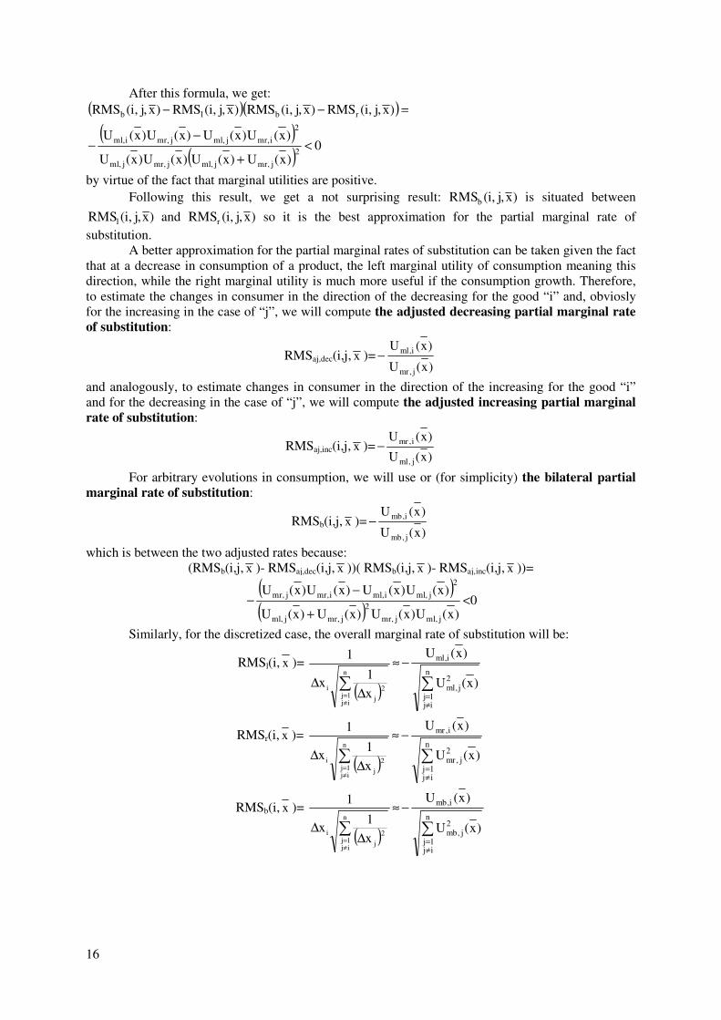
After this formula, we get:

( )( )( )

( ) 0)x(U)x(U)x(U)x(U

)x(U)x(U)x(U)x(U

)x,j,i(RMS)x,j,i(RMS)x,j,i(RMS)x,j,i(RMS

2

j,mrj,mlj,mrj,ml

2

i,mrj,mlj,mri,ml

rblb

<+

−−

=−−

by virtue of the fact that marginal utilities are positive.

Following this result, we get a not surprising result: )x,j,i(RMSb is situated between

)x,j,i(RMSl and )x,j,i(RMSr so it is the best approximation for the partial marginal rate of

substitution.

A better approximation for the partial marginal rates of substitution can be taken given the fact

that at a decrease in consumption of a product, the left marginal utility of consumption meaning this

direction, while the right marginal utility is much more useful if the consumption growth. Therefore,

to estimate the changes in consumer in the direction of the decreasing for the good “i” and, obviosly

for the increasing in the case of “j”, we will compute the adjusted decreasing partial marginal rate

of substitution:

RMSaj,dec(i,j, x )=)x(U

)x(U

j,mr

i,ml−

and analogously, to estimate changes in consumer in the direction of the increasing for the good “i”

and for the decreasing in the case of “j”, we will compute the adjusted increasing partial marginal

rate of substitution:

RMSaj,inc(i,j, x )=)x(U

)x(U

j,ml

i,mr−

For arbitrary evolutions in consumption, we will use or (for simplicity) the bilateral partial

marginal rate of substitution:

RMSb(i,j, x )=)x(U

)x(U

j,mb

i,mb−

which is between the two adjusted rates because:

(RMSb(i,j, x )- RMSaj,dec(i,j, x ))( RMSb(i,j, x )- RMSaj,inc(i,j, x ))=

( )( ) )x(U)x(U)x(U)x(U

)x(U)x(U)x(U)x(U

j,mlj,mr

2

j,mrj,ml

2

j,mli,mli,mrj,mr

+

−− <0

Similarly, for the discretized case, the overall marginal rate of substitution will be:

RMSl(i, x )=

( )∑≠= ∆

∆n

ij1j

2

j

ix

1x

1 ≈

∑≠=

−n

ij1j

2j,ml

i,ml

)x(U

)x(U

RMSr(i, x )=

( )∑≠= ∆

∆n

ij1j

2

j

ix

1x

1 ≈

∑≠=

−n

ij1j

2j,mr

i,mr

)x(U

)x(U

RMSb(i, x )=

( )∑≠= ∆

∆n

ij1j

2

j

ix

1x

1 ≈

∑≠=

−n

ij1j

2j,mb

i,mb

)x(U

)x(U

17

7. EXEMPLES OF PREFERENCES

7.1. Perfectly substitutable goods We say that n goods are perfectly substitutable if the utility function is linear, i.e.:

U(x1,...,xn)=a1x1+...+anxn, ai>0, i= n,1

In this case, we have: Um,i=i

x

U

∂∂

=ai, i= n,1 and the partial substitution marginal rate is:

RMS(i,j, x )=j

i

a

a−

whereas the overall marginal rate of substitution is:

RMS(i, x )=

∑≠=

−n

ij1j

2

j

i

a

a

Also the marginal substitution hyperplane between good “i” and the other goods has the

equation:

0aya i

n

ij1j

jj =+∑≠=

We can see in this case that both the marginal rate of substitution and the overall are constant.

This implies that whatever is the level of consumption, the substitutability between any two goods,

caeteris paribus, has the same factor.

The minimal vector of the i-th good substitution is:

( )ni1n

ij1j

2j

i a,...,a,...,a

a

a

∑≠=

−

7.2. Independent goods from the utility point of view

We will say that n goods are independent from utility the point of view if the utility function

is:

U(x1,...,xn)=f1(x1)+...+fn(xn), with fi∈C2(0,∞), if ′′ ≤0, i= n,1 and f1(0)+...+fn(0)=0

In this case we have:

Um,i=i

x

U

∂∂

= if ′ , i= n,1 , 2

i

2

x

U

∂∂

= if ′′ , i= n,1 , 0xx

U

ji

2

=∂∂

∂ ∀i≠j

Because d2U=∑

=

′′n

1j,i

2

iidxf follows that U is concave.

Before proceeding further, let note that in the case of the linearity of functions fi (fi(xi)=aixi,

ai>0) the goods become perfectly substitutable.

The partial substitution marginal rate is: RMS(i,j, x )=)x(f

)x(f

jj

ii

′′

− and the overall marginal rate

of substitution: RMS(i, x )=

∑≠=

′

′−

n

ij1j

j

2

j

ii

)x(f

)x(f.

Also the marginal substitution hyperplane between good “i” and the other goods has the

equation:

0)x(fy)x(f ii

n

ij1j

jjj =′+′∑≠=

18

The minimal vector of the i-th good substitution is therefore:

( ))x(f),...,x(f),...,x(f

)x(f

)x(fnnii11n

ij1j

j

2

j

ii ′′′′

′−∑≠=

7.3. Separable goods from the utility point of view We will say that n goods are separable from the utility point of view if the utility function is:

U(x1,...,xn)=f1(x1)⋅...⋅fn(xn), cu fi∈C2(0,∞), fi(x)>0 ∀x>0, if ′′ ≤0, i= n,1 , f1(0)⋅...⋅fn(0)=0

and the quadratic form:

H= ∑∑==

ξξ′′

+ξ′′ n

1j,iji

ji

jin

1i

2

i

i

i

ff

ff

f

f

is negatively defined.

In this case, we have:

Um,i=i

x

U

∂∂

= ni1 f...f...f ′ =Ui

i

f

f ′, i= n,1 ,

2

i

2

x

U

∂∂

= ni1 f...f...f ′′ =Ui

i

f

f ′′, i= n,1 , nji1

ji

2

f...f...f...fxx

U ′′=∂∂

∂=U

ji

ji

ff

ff ′′ ∀i≠j

From the fact that H is a negative defined quadratic form, it follows that U is concave.

The partial substitution marginal rate is: RMS(i,j, x )=)x(f)x(f

)x(f)x(f

iijj

jjii

′

′− and the overall marginal

rate of substitution is: RMS(i, x )=

∑≠=

′

′−

n

ij1j j

2

j

j

2

j

ii

ii

)x(f

)x(f)x(f

)x(f.

Also the marginal substitution hyperplane between the i-th good and the others has the

equation:

0)x(f

)x(fy

)x(f

)x(f

ii

iin

ij1j

j

jj

jj =′

+′

∑≠=

and the minimal vector of goods substitution:

′′′′

′−

∑≠=

)x(f

)x(f,...,

)x(f

)x(f,...,

)x(f

)x(f

)x(f

)x(f)x(f

)x(f

nn

nn

ii

ii

11

11

n

ij1j j

2j

j

2

j

ii

ii

Let consider, as a particular example, the Cobb-Douglas function:

U(x1,x2,...,xn)=n1

n1x...x

αα cu αi>0, ∑

=α

n

1ii ≤1

Computing the marginal partial rate of substitution, we get: RMS(i,j, x )=ij

ji

x

x

α

α− and the

overall marginal rate of substitution: RMS(i, x )=

∑≠=

α

α−

n

ij1j

2

j

2

j

i

i

xx

. Also the marginal substitution

hyperplane between the i-th good and the others has the equation:

0x

yx i

in

ij1j

j

j

j =α

+α

∑≠=

8. CONCLUSIONS

The onset of the notions of preference in selecting baskets of goods and the utility on the other

hand impose a number of precautions both conceptual and technical. Even if such an axiomatic

19

constraint will lead to “loss” of some important cases, the axiomatisation gives, on the one hand, rigor

to the theory and, on the other hand, generates new situations by using norms more or less exotic (1-

norm, ∞-norm, p-norms).

On the other hand, the analysis of the concurrent consumption of n goods variance, decontrols

the theory from “caeteris paribus” constraints, getting interesting conclusions and making a first step

towards the overall analysis of the microeconomic phenomenon. The n-dimensional approach to the

basic phenomena, even if it is based on a number of notions of n-dimensional Euclidean geometry or,

in the overall treatment of the utility function, a series of differential geometry results, adds generality

and more accurate simulation of microeconomic reality.

Also the treatment of the marginal utility to the left, right or bilateral as well as marginal rates

of substitution of different types, introduced above, allows enrichment practical conclusions,

eliminating the classical mono-directional variations like the discretized derivative derived as the

average of discretized left and right derivatives gives more precise information on the behavior of a

function.

REFERENCES 1. Chiang A.C. (1984), Fundamental Methods of Mathematical Economics, McGraw-Hill Inc.

2. Ioan C.A., Ioan G. (2011), A generalisation of a class of production functions, Applied economics

letters, 18, pp. 1777-1784

3. Ioan C.A., Ioan G. (2011), The Extreme of a Function Subject to Restraint Conditions, Acta

Oeconomica Danubius, 7, 3, pp. 203-207

4. Stancu S. (2006), Microeconomics, Ed. Economica, Bucharest

5. Varian H.R. (2006), Intermediate Microeconomics, W.W.Norton & Co.