arX

iv:c

ond-

mat

/040

9644

v1 [

cond

-mat

.oth

er]

24

Sep

2004

Correlated geminal wave function for molecules: an efficient resonating valence bond

approach

Michele Casula,∗ Claudio Attaccalite,† and Sandro Sorella‡

International School for Advanced Studies (SISSA) Via Beirut 2,4 34014 Trieste ,Italy and INFM Democritos National Simulation Center, Trieste, Italy

(Dated: December 30, 2013)

We show that a simple correlated wave function, obtained by applying a Jastrow correlationterm to an Antisymmetrized Geminal Power (AGP), based upon singlet pairs between electrons, isparticularly suited for describing the electronic structure of molecules, yielding a large amount of thecorrelation energy. The remarkable feature of this approach is that, in principle, several ResonatingValence Bonds (RVB) can be dealt simultaneously with a single determinant, at a computational costgrowing with the number of electrons similarly to more conventional methods, such as Hartree-Fock(HF) or Density Functional Theory (DFT). Moreover we describe an extension of the StochasticReconfiguration (SR) method, that was recently introduced for the energy minimization of simpleatomic wave functions. Within this extension the atomic positions can be considered as furthervariational parameters, that can be optimized together with the remaining ones. The method isapplied to several molecules from Li2 to benzene by obtaining total energies, bond lengths andbinding energies comparable with much more demanding multi configuration schemes.

I. INTRODUCTION

The comprehension of the nature of the chemical bonddeeply lies on quantum mechanics; since the seminal workby Heitler and London [1], very large steps have beenmade towards the possibility to predict the quantitativeproperties of the chemical compounds from a theoreticalpoint of view. Mean field theories, such as HF have beensuccessfully applied to a wide variety of interesting sys-tems, although they fail in describing those in which thecorrelation is crucial to characterize correctly the chemi-cal bonds. For instance the molecular hydrogen H2, thesimplest and first studied molecule, is poorly described bya single Slater determinant in the large distance regime,which is the paradigm of a strongly correlated bond; in-deed, in order to avoid expensive energy contributions -the so called ionic terms - that arise from two electrons ofopposite spin surrounding the same hydrogen atom, oneneeds at least two Slater determinants to deal with a spinsinglet wave function containing bonding and antibond-ing molecular orbitals. Moreover at the bond distance itturns out that the resonance between those two orbitalsis important to yield accurate bond length and bindingenergy, as the correct rate between the ionic and covalentcharacter is recovered. Another route that leads to thesame result is to deal with an AGP wave function, whichincludes the correlation in the geminal expansion; Barbi-ellini in Ref. 2 gave an illuminating example of the beautyof this approach solving merely the simple problem of theH2 molecule.

On the other hand the variational methods based onthe Configuration Interaction (CI) technique, which is

∗casula@sissa.it†claudio@freescience.info‡sorella@sissa.it

able to take into account many Slater determinants, havebeen shown to be successful for small molecules (e.g. Be2[3]). In these cases it is indeed feasible to enlarge thevariational basis up to the saturation, the electron cor-relation properties are well described and consequentlyall the chemical properties can be predicted with ac-curacy. However, for interesting systems with a largenumber of atoms this approach is impossible with a rea-sonable computational time. Coming back to the H2

paradigm, it is straightforward to show that a gas withN H2 molecules, in the dilute limit, can be dealt accu-rately only with 2N Slater determinants, otherwise oneis missing important correlations due to the antibondingmolecular orbital contributions, referred to each of the NH2 molecules. Therefore, if the accuracy in the total en-ergy per atom is kept fixed, a CI-like approach does notscale polynomially with the number of atoms. Althoughthe polynomial cost of these Quantum Chemistry algo-rithms - ranging from N5 to N7 - is not prohibitive, aloss of accuracy, decreasing exponentially with the num-ber of atoms is always implied, at least in their simplestvariational formulations. This is related to the loss of sizeconsistency of a truncated CI expansion. On the otherhand, this problem can be overcome by coupled clustermethods, that however in their practical realization arenot variational[4].

An alternative approach, not limited to smallmolecules, is based on DFT. This theory is in principleexact, but its practical implementation requires an ap-proximation for the exchange and correlation function-als based on first principles, like the Local Density ap-proximation (LDA) and its further gradient corrections(GGA), or on semi empirical approaches, like BLYP andB3LYP. For this reason, even though much effort hasbeen made so far to go beyond the standard functionals,DFT is not completely reliable in those cases in whichthe correlation plays a crucial role. Indeed it fails in de-scribing HTc superconductors and Mott insulators, and

2

in predicting some transition metal compounds proper-ties, whenever the outermost atomic d-shell is near-half-filled, as for instance in the high potential iron proteins(HiPIP)[5]. AlsoH2 molecule in the large distance regimemust be included in that list, since the large distanceBorn-Oppenheimer energy surface, depending on Van derWaals forces, is not well reproduced by the standard func-tionals, although recently some progress has been madeto include these important contributions[6].

Quantum Monte Carlo (QMC) methods are alternativeto the previous ones and until now they have been mainlyused in two versions:

• Variational Monte Carlo (VMC) applied to a wavefunction with a Jastrow factor that fulfills the cuspconditions and optimizes the convergence of the CIbasis[7, 8];

• Diffusion Monte Carlo (DMC) algorithm used toimprove, often by a large amount, the correlationenergy of any given variational guess in an auto-matic manner [9].

Hereafter we want to show that a large amount ofthe correlation energy can be obtained with a single de-terminant, using a size-consistent AGP-Jastrow (JAGP)wave function. Clearly our method is approximate and insome cases not yet satisfactory, but in a large number ofinteresting molecules we obtain results comparable andeven better than multi determinants schemes based onfew Slater determinants per atom that are affordable byQMC only for rather small molecules.

Moreover, we have extended the standard SR methodto treat the atomic positions as further variational pa-rameters. This improvement, together with the possi-bility to work with a single determinant, has allowedus to perform a structural optimization in a non triv-ial molecule like the benzene radical cation, reaching thechemical accuracy with an all-electron and feasible vari-ational approach.

The paper is organized as follows: In Sec. II we in-troduce the variational wave function, that is expandedover a set of non orthogonal atomic orbitals both in thedeterminantal AGP and the Jastrow part. This basis setis consistently optimized using the method described inSec. III that, as mentioned before, allows also the geom-etry optimization. Results and discussions are presentedin the remaining sections.

II. FUNCTIONAL FORM OF THE WAVE

FUNCTION

In this paper we are going to extend the applicationof the JAGP wave function, already used to study someatomic systems [10]. We generalize its functional formin order to describe the electronic structure of a genericcluster containing several nuclei. With the aim to deter-mine a variational wave function, suitable for a complex

electronic system, it is important to satisfy, as we re-quire in the forthcoming chapters, the ”size consistency”property: if we smoothly increase the distance betweentwo regions A and B each containing a given numberof atoms, the many-electron wave function Ψ factorizesinto the product of space-disjoint terms Ψ = ΨA

⊗

ΨB

as long as the interaction between the electrons couplingthe different regions A and B can be neglected. In thislimit the total energy of the wave function approachesthe sum of the energies corresponding to the two space-disjoint regions. This property, that is obviously validfor the exact many-electron ground state, is not alwaysfulfilled by a generic variational wave function.

Our variational wave function is defined by the prod-uct of two terms, namely a Jastrow J and an antisym-metric part (Ψ = JΨAGP ). If the former is an explicitcontribution to the dynamic electronic correlation, thelatter is able to treat the non dynamic one arising fromnear degenerate orbitals through the geminal expansion.Therefore our wave function is highly correlated and it isexpected to give accurate results especially for molecularsystems. The Jastrow term is further split into a twobody and a three body factors, J = J2J3, described inthe following subsections after the AGP part.

A. Pairing determinant

As is well known, a simple Slater determinant providesthe exact exchange electron interaction but neglects theelectronic correlation, which is by definition the missingenergy contribution. In the past different strategies wereproposed to go beyond Hartree-Fock theory. In particu-lar a sizable amount of the correlation energy is obtainedby applying to a Slater determinant a so called Jastrowterm, that explicitly takes into account the pairwise in-teraction between electrons. QMC allows to deal withthis term in an efficient way[11]. On the other hand,within the Quantum Chemistry community AGP is a wellknown ansatz to improve the HF theory, because it im-plicitly includes most of the double-excitations of an HFstate.

Recently we proposed a new trial function for atoms,that includes both the terms. Only the interplay betweenthem yields in some cases, like Be or Mg, an extremelyaccurate description of the correlation energy. In thiswork we extend this promising approach to a number ofsmall molecular systems with known experimental prop-erties, that are commonly used for testing new numericaltechniques.

The major advantage of this approach is the inclusionof many CI expansion terms with the computational costof a single determinant,

that allow us to extend the calculation with a full struc-tural optimization up to benzene, without a particularlyheavy computational effort on a single processor machine.For an unpolarized system containing N electrons (thefirst N/2 coordinates are referred to the up spin elec-

3

trons) the AGP wave function is a N2 × N

2 pairing matrixdeterminant, which reads:

ΨAGP (r1, ..., rN ) = det(

ΦAGP (ri, rj+N/2))

, (1)

and the geminal function is expanded over an atomic ba-sis:

ΦAGP (r↑, r↓) =∑

l,m,a,b

λl,ma,b φa,l(r

↑)φb,m(r↓), (2)

where indices l,m span different orbitals centered onatoms a, b, and i,j are coordinates of spin up and downelectrons respectively. The geminal functions may beviewed as an extension of the simple HF wavefunction,based on molecular orbitals, and in fact the geminal func-tion coincide with HF only when the number M of nonzero eigenvalues of the λ matrix is equal to N/2. Indeedthe general function 2 can be written in diagonal formafter an appropriate transformation:

ΦAGP (r↑, r↓) =

M∑

k

λkφk(r↑)φk(r↓), (3)

where φk(r) =∑

j,a µk,j,aφj,a(r) are just the molecular

orbitals of the HF theory whenever M = N/2. Noticethat with respect to our previous pairing function for-mulation also off-diagonal elements are now included inthe λ matrix, which must be symmetric in order to de-fine a singlet spin orbital state. Moreover it allows one toeasily fulfill other system symmetries by setting the ap-propriate equalities among different λl,m. For instancein homo-nuclear diatomic molecules, the invariance un-der reflection in the plane perpendicular to the molecularaxis yields the following relation:

λa,bm,n = (−1)pm+pnλb,a

m,n, (4)

where pm is the parity under reflection of the m−th or-bital.

Another important property of this formalism is thepossibility to describe resonating bonds present in manystructures, like benzene. A λa,b

m,n different from zero rep-resents a chemical bond formed by the linear combinationof the m-th and n-th orbitals belonging to a-th and b-thnuclei. It turns out that resonating bonds can be well de-scribed through the geminal expansion switching on theappropriate λa,b

m,n coefficients: the relative weight of eachbond is related to the amplitude of its λ.

Also the spin polarized molecules can be treated withinthis framework, by using the spin generalized version ofthe AGP (GAGP), in which the unpaired orbitals are ex-panded as well as the paired ones over the same atomicbasis employed in the geminal[12]. As already mentionedin the introduction of this chapter, the size consistencyis an appealing feature of the AGP term. Strictly speak-ing, the AGP wave function is certainly size consistentwhen both the compound and the separated fragmentshave the minimum possible total spin, because the gem-inal expansion contains both bonding and antibonding

contributions, that can mutually cancel the ionic termarising in the asymptotically separate regime. Moreoverthe size consistency of the AGP, as well as the one of theHartree-Fock state, holds in all cases in which the spinof the compound is the sum of the spin of the fragments.However, similarly to other approaches[4], for spin polar-ized systems the size consistency does not generally hold,and, in such cases, it may be important go beyond a singleAGP wave function. Nevertheless we have experiencedthat a single reference AGP state is able to describe ac-curately the electronic structure of the compound aroundthe Born-Oppenheimer minimum even in the mentionedpolarized cases, such as in the oxygen dimer.

The last part of this section is devoted to the nuclearcusp condition implementation. A straightforward cal-culation shows that the AGP wave function fulfills thecusp conditions around the nucleus a if the following lin-ear system is satisfied:

(1s,2s)∑

j

λj,j′

a,b φ′a,j(r = Ra) = −Za

∑

c,j

λj,j′

c,b φc,j(r = Ra),

(5)for all b and j′; in the LHS the caret denotes the sphericalaverage of the orbital gradient. The system can be solvediteratively during the optimization processes, but if weimpose that the orbitals satisfy the single atomic cuspconditions, it reduces to:

∑

c( 6=a),j

λj,j′

c,b φc,j(Ra) = 0, (6)

and because of the exponential orbital damping, if thenuclei are not close together each term in the previousequations is very small, of the order of exp(−|Ra −Rc|).Therefore, with the aim of making the optimizationfaster, we have chosen to use 1s and 2s orbitals satisfy-ing the atomic cusp conditions and to disregard the sum(6) in Eq. 5. In this way, once the energy minimum isreached, also the molecular cusp conditions (5) are ratherwell satisfied.

B. Two body Jastrow term

As it is well known the Jastrow term plays a crucialrole in treating many body correlation effects. One of themost important correlation contributions arises from theelectron-electron interaction. Therefore it is worth us-ing at least a two-body Jastrow factor in the trial wavefunction. Indeed this term reduces the electron coales-cence probability, and so decreases the average value ofthe repulsive interaction. The two-body Jastrow functionreads:

J2(r1, ..., rN ) = exp

N∑

i<j

u(rij)

, (7)

4

where u(rij) depends only on the relative distance rij =|ri − rj | between two electrons and allows to fulfill thecusp conditions for opposite spin electrons as long asu(rij) → rij

2 for small electron-electron distance. Thepair correlation function u can be parametrized success-fully by few variational parameters. We have adoptedtwo main functional forms. The first is similar to the onegiven by Ceperley [13]:

u(r) =F

2

(

1 − e−r/F)

, (8)

with F being a free variational parameter. This formfor u is particularly convenient whenever atoms are veryfar apart at distances much larger than F , as it allowsto obtain good size consistent energies, approximatelyequal to the sum of the atomic contributions, withoutchanging the other parts of the wave function with anexpensive optimization. Within the functional form (8),it is assumed that the long range part of the Jastrow,decaying as a power of the distance between atoms, isincluded in the 3-body Jastrow term described in thenext subsection. The second form of the pair functionu, particularly convenient at the chemical bond distance,where we performed most of the calculations, is the oneused by Fahy [7]:

u(r) =r

2(1 + br), (9)

with a different variational parameter b.In both functional forms the cusp condition for antipar-

allel spin electrons is satisfied, whereas the one for paral-lel spins is neglected in order to avoid the spin contamina-tion. This allows to remove the singularities of the localenergy due to the collision of two opposite spin electrons,yielding a smaller variance and a more efficient VMC cal-culation. Moreover, due to the Jastrow correlation, anexact property of the ground state wave function is re-covered without using many Slater determinants, thusconsiderably simplifying the variational parametrizationof a correlated wave function.

C. Three Body Jastrow term

In order to describe well the correlation between elec-trons the simple Jastrow factor is not sufficient. Indeedit takes into account only the electron-electron separa-tion and not the individual electronic position ri and rj .It is expected that close to nuclei the electron correla-tion is not accurately described by a translationally in-variant Jastrow, as shown by different authors, see forinstance Ref. 14. For this reason we introduce a fac-tor, often called three body (electron-electron-nucleus)Jastrow, that explicitly depends on both the electronicpositions ri and rj . The three body Jastrow is chosen tosatisfy the following requirements:

• The cusp conditions set up by the two-body Jas-trow term and by the AGP are preserved.

• It does not distinguish the electronic spins other-wise causing spin contamination.

• Whenever the atomic distances are large it factor-izes into a product of independent contributions lo-cated near each atom, an important requirement tosatisfy the size consistency of the variational wavefunction.

Analogously to the pairing trial function in Eq. 2 wedefine a three body factor as:

J3(r1, ..., rN ) = exp

∑

i<j

ΦJ (ri, rj)

ΦJ(ri, rj) =∑

l,m,a,b

ga,bl,mψa,l(ri)ψb,m(rj), (10)

where indices l and m indicate different orbitals locatedaround the atoms a and b respectively. Each Jastroworbital ψa,l(r) is centered on the corresponding atomicposition Ra. We have used Gaussian and exponential or-bitals multiplied by appropriate polynomials of the elec-tronic coordinates, related to different spherical harmon-ics with given angular momentum, as in the usual Slaterbasis. Analogously to the geminal function ΦAGP , when-ever the one particle basis set {ψa,i} is complete the ex-pansion (10) is also complete for the generic two particlefunction ΦJ (r, r′). In the latter case, however, the oneparticle orbitals have to behave smoothly close to thecorresponding nuclei, namely as:

ψa,i(r) − ψa,i(Ra) ≃ |r − Ra|2, (11)

or with larger power, in order to preserve the nuclearcusp conditions (5).

For the s-wave orbitals we have found energeticallyconvenient to add a finite constant cl/(N −1). As shownin the Appendix B, a non zero value of the constant clfor such orbitals ψa,l is equivalent to include in the wavefunction a size consistent one body term. As pointed outin Ref. 16, it is easier to optimize a one body term im-plicitly present in the 3-body Jastrow factor, rather thanincluding more orbitals in the determinantal basis set.

The chosen form for the 3-body Jastrow (10) is simi-lar to one used by Prendergast et al. [15] and has veryappealing features: it easily allows including the symme-

tries of the system by imposing them on the matrix ga,bl,m

exactly as it is possible for the pairing part (e.g. by re-placing λa,b

m,n with ga,bm,n in Eq. 4). It is size consistent,

namely the atomic limit can be smoothly recovered with

the same trial function when the matrix terms ga,bl,m for

a 6= b approach zero in this limit. Notice that a small non

zero value of ga,bl,m for a 6= b acting on p-wave orbitals can

correctly describe a weak interaction between electronssuch as the the Van der Waals forces.

5

III. OPTIMIZATION METHOD

We have used the Stochastic Reconfiguration (SR)method already described in Ref. 17, that allows to min-imize the energy expectation value of a variational wavefunction containing many variational parameters in anarbitrary functional form. The basic ingredient for thestochastic minimization of the wave function Ψ deter-mined by p variational parameters {α0

k}k=1,...,p, is thesolution of the linear system:

p∑

k=0

sj,k∆αk = 〈Ψ|Ok(ΛI −H)|Ψ〉, (12)

where the operators Ok are defined on each N electronconfiguration x = {r1, . . . , rN} as the logarithmic deriva-tives with respect to the parameters αk:

Ok(x) =∂

∂αkln Ψ(x) for k > 0, (13)

while for k = 0 Ok is the identity operator equal to oneon all the configurations. The (p + 1) × (p + 1) matrix

sk,j is easily expressed in terms of these operators:

sj,k =〈Ψ|OjOk|Ψ〉

〈Ψ|Ψ〉 , (14)

and is calculated at each iteration through a standardvariational Monte Carlo sampling ; the single iterationconstitutes a small simulation that will be referred in thefollowing as “bin”. After each bin the wave function pa-rameters are iteratively updated (αk → αk +∆αk/∆α0),and the method is convergent to an energy minimum forlarge enough Λ. Of course for particularly simple func-tional form of Ψ(x), containing e.g. only linear CI co-efficients, much more efficients optimization schemes doexist [18].

SR is similar to a standard steepest descent (SD)calculation, where the expectation value of the energy

E(αk) = 〈Ψ|H|Ψ〉〈Ψ|Ψ〉 is optimized by iteratively changing the

parameters αi according to the corresponding derivativesof the energy (generalized forces):

fk = − ∂E

∂αk= −〈Ψ|OkH +HOk + (∂αk

H)|Ψ〉〈Ψ|Ψ〉 + 2

〈Ψ|Ok|Ψ〉〈Ψ|H |Ψ〉〈Ψ|Ψ〉2 , (15)

namely:

αk → αk + ∆tfk. (16)

∆t is a suitable small time step, which can be taken fixedor determined at each iteration by minimizing the energyexpectation value. Indeed the variation of the total en-ergy ∆E at each step is easily shown to be negative forsmall enough ∆t because, in this limit

∆E = −∆t∑

i

f2i +O(∆t2).

Thus the method certainly converges at the minimumwhen all the forces vanish. Notice that in the defini-tion of the generalized forces (15) we have generally as-sumed that the variational parameters may appear also inthe Hamiltonian. This is particularly important for thestructural optimization since the atomic positions thatminimize the energy enter both in the wave function andin the potential.

In the following we will show that similar consider-ations hold for the SR method, that can be thereforeextended to the optimization of the geometry. Indeed,by eliminating the equation with index k = 0 from thelinear system (12), the SR iteration can be written in a

form similar to the steepest descent:

αi → αi + ∆t∑

k

s−1i,kfk (17)

where the reduced p× p matrix s is:

sj,k = sj,k − sj,0s0,k (18)

and the ∆t value is given by:

∆t =1

2(Λ − 〈Ψ|H|Ψ〉〈Ψ|Ψ〉 − ∑

k>0 ∆αksk,0). (19)

¿From the latter equation the value of ∆t changes duringthe simulation and remains small for large enough energyshift Λ. However, using the analogy with the steepestdescent, convergence to the energy minimum is reachedalso when the value of ∆t is sufficiently small and is keptconstant for each iteration. Indeed the energy variationfor a small change of the parameters is:

∆E = −∆t∑

i,j

s−1i,j fifj .

It is easily verified that the above term is always negativebecause the reduced matrix s, as well as s−1, is positive

6

definite, being s an overlap matrix with all positive eigen-values.

For a stable iterative method, such as the SR or theSD one, a basic ingredient is that at each iteration thenew parameters α′ are close to the previous α accord-ing to a prescribed distance. The fundamental differencebetween the SR minimization and the standard steepestdescent is just related to the definition of this distance.For the SD it is the usual one defined by the Cartesianmetric ∆α =

∑

k |α′k − αk|2, instead the SR works cor-

rectly in the physical Hilbert space metric of the wavefunction Ψ, yielding ∆α =

∑

i,j si,j(α′i − αi)(α

′j − αj),

namely the square distance between the two normalizedwave functions corresponding to the two different sets ofvariational parameters {α′} and {αk}. Therefore, fromthe knowledge of the generalized forces fk, the most con-venient change of the variational parameters minimizesthe functional ∆E+Λ∆α, where ∆E is the linear changein the energy ∆E = −

∑

i fi(α′i−αi) and Λ is a Lagrange

multiplier that allows a stable minimization with smallchange ∆α of the wave function Ψ. The final iteration(17) is then easily obtained.

The advantage of SR compared with SD is obviousbecause sometimes a small change of the variational pa-rameters correspond to a large change of the wave func-tion, and the SR takes into account this effect throughthe Eq. 17. In particular the method is useful when anon orthogonal basis set is used as we have done in thiswork. Indeed by using the reduced matrix s it is alsopossible to remove from the calculation those parame-ters that imply some redundancy in the variational space.As shown in the Appendix A, a more efficient change inthe wave function can be obtained by updating only thevariational parameters that remain independent withina prescribed tolerance, and therefore, by removing theparameters that linearly depend on the others. A morestable minimization is obtained without spoiling the ac-curacy of the calculation. A weak tolerance criteriumǫ ≃ 10−3, provides a very stable algorithm even when thedimension of the variational space is large. For a smallatomic basis set, by an appropriate choice of the Jastrowand Slater orbitals, the reduced matrix s is always verywell conditioned even for the largest system studied, andthe above stabilization technique is not required. Insteadthe described method is particularly important for theextension of QMC to complex systems with large num-ber of atoms and/or higher level of accuracy, because inthis case it is very difficult to select - e.g. by trial anderror - the relevant variational parameters, that allow awell conditioned matrix s for a stable inversion in (17).

A. Setting the SR parameters

In this work, instead of setting the constant Λ, wehave equivalently chosen to determine ∆t by verifyingthe stability and the convergence of the algorithm atfixed ∆t value, which can be easily understood as an

inverse energy scale. The simulation is stable when-ever 1/∆t > Λcut, where Λcut is an energy cutoff thatis strongly dependent on the chosen wave function andis generally weakly dependent on the bin length. When-ever the wave function is too much detailed, namely hasa lot of variational freedom, especially for the high en-ergy components of the core electrons, the value of Λcut

becomes exceedingly large and too many iterations arerequired for obtaining a converged variational wave func-tion. In fact a rough estimate of the corresponding num-ber of iterations P is given by P∆t >> 1/G, where G isthe typical energy gap of the system, of the order of fewelectron Volts in small atoms and molecules. Within theSR method it is therefore extremely important to workwith a bin length rather small, so that many iterationscan be performed without much effort.

In a Monte Carlo optimization framework the forces fk

are always determined with some statistical noise ηk, andby iterating the procedure several times with a fixed binlength the variational parameters will fluctuate aroundtheir mean values. These statistical fluctuations are sim-ilar to the thermal noise of a standard Langevin equation:

∂tαk = fk + ηk, (20)

where

〈ηk(t)ηk′ (t′)〉 = 2Tnoiseδ(t− t′)δk,k′ . (21)

The variational parameters αk, averaged over theLangevin simulation time (as for instance in Fig.1 fort > 2H−1), will be close to the true energy minimum, butthe corresponding forces fk = −∂αk

E will be affected bya bias that scales to zero with the thermal noise Tnoise,due to the presence of non quadratic terms in the energylandscape.

Within a QMC scheme, one needs to estimate Tnoise,by increasing the bin length as clearly Tnoise ∝1/Bin length, because the statistical fluctuations of theforces, obviously decreasing by increasing the bin length,are related to the thermal noise by Eq. 21. Thus there isan optimal value for the bin length, which guarantees afast convergence and avoid the forces to be biased withinthe statistical accuracy of the sampling.

An example is shown in Fig. 1 for the optimization ofthe Be atom, using a DZ basis both for the geminal andthe three-body Jastrow part. The convergence is reachedin about 1000 iteration with ∆t = 0.005H−1. However,in this case it is possible to use a small bin length, yield-ing a statistical accuracy in the energy much poorer thanthe final accuracy of about 0.05mH . This is obtained byaveraging the variational parameters in the last 1000 iter-ations, when they fluctuate around a mean value, allow-ing a very accurate determination of the energy minimumwhich satisfies the Euler conditions, namely with fk = 0for all parameters. Those conditions have been tested byan independent Monte Carlo simulation about 600 timeslonger than the bin used during the minimization. As

7

0

2

4

6

8

10

0 500 1000 1500 2000 2500 3000

AGP

# Iterations

0

2

4

6

8

10

0 500 1000 1500 2000 2500 3000

AGP

# Iterations

Z11s

Z21s

Z12s

Z22s

Z12p

Z22p

0

1

2

3

4

Jastrow

0

1

2

3

4

Jastrow

Z11s

Z12s

Z12p

Z22p

FIG. 1: Example of the convergence of the SR method for the variational parameters of the Be atom, as a function of thenumber of stochastic iterations. In the upper(lower) panel the Jastrow (geminal) parameters are shown. For each iteration, avariational Monte Carlo calculation is employed with a bin containing 15000 samples of the energy, yielding at the equilibrium astandard deviation of ≃ 0.0018H . For the first 200 iteration ∆t = 0.00125H−1 , for the further 200 iterations ∆t = 0.0025H−1 ,whereas for the remaining ones ∆t = 0.005H−1.

shown in Fig. 2 the Euler conditions are fulfilled withinstatistical accuracy even when the bin used for the mini-mization is much smaller than the overall simulation. Onthe other hand if the bin used is too small, as we havealready pointed out, the averaging of the parameters isaffected by a sizable bias.

0.0 0.2-0.002

-0.001

0.000

- dE

/ d Z

2 2p

1000/Bin lenght

Be atom

FIG. 2: Calculation of the derivative of the energy with re-spect to the second Z in the 2p orbital of the geminal functionfor the Be atom. The calculation of the force was obtained,at fixed variational parameters, by averaging over 107 sam-ples, allowing e.g. a statistical accuracy in the total energyof 0.07mH . The variational parameters have been obtainedby an SR minimization with fixed bin length shown in thex label. The parameter considered has the largest deviationfrom the Euler conditions.

Whenever it is possible to use a relatively small bin inthe minimization, the apparently large number of iter-ations required for equilibration does not really matter,because a comparable amount of time has to be spentin the averaging of the variational parameters, as shownin Fig. 1. The comparison shown in the Ref. 19 aboutthe number of the iterations required, though is clearlyrelevant for a deterministic method, is certainly incom-plete for a statistical method, because in the latter casean iteration can be performed in principle in a very shorttime, namely with a rather small bin.

It is indeed possible that for high enough accuracy thenumber of iterations needed for the equilibration becomesnegligible from the computational point of view. In factin order to reduce, e.g. by a factor ten, the accuracy inthe variational parameters, a bin ten times larger is re-quired for decreasing the thermal noise Tnoise by the samefactor, whereas a statistical average 100 times longer isindeed necessary to reduce the statistical errors of thevariational parameters by the same ratio. This meansthat the fraction of time spent for equilibration becomesten times smaller compared with the less accurate simu-lation.

B. Structural optimization

In the last few years remarkable progresses have beenmade to develop Quantum Monte Carlo (QMC) tech-niques which are able in principle to perform struc-tural optimization of molecules and complex systems[20, 21, 22]. Within the Born-Oppenheimer approxima-tion the nuclear positions Ri can be considered as further

8

variational parameters included in the set {αi} used forthe SR minimization (17) of the energy expectation value.For clarity, in order to distinguish the conventional varia-tional parameters from the ionic positions, in this sectionwe indicate with {ci} the former ones, and with Ri thelatter ones. It is understood that Rν

i = αk, where aparticular index k of the whole set of parameters {αi}corresponds to a given spatial component (ν = 1, 2, 3) ofthe i−th ion. Analogously the forces (15) acting on theionic positions will be indicated by capital letters withthe same index notations.

The purpose of the present section is to computethe forces F acting on each of the M nuclear positions{R1, . . . ,RM}, being M the total number of nuclei in thesystem:

F(Ra) = −∇RaE({ci},Ra), (22)

with a reasonable statistical accuracy, so that the itera-tion (17) can be effective for the structural optimization.In this work we have used a finite difference operator∆

∆Rafor the evaluation of the force acting on a given

nuclear position a:

F(Ra) = − ∆

∆RaE (23)

= −E(Ra + ∆Ra) − E(Ra − ∆Ra)

2∆R+O(∆R2)

where ∆Ra is a 3 dimensional vector. Its length ∆Ris chosen to be 0.01 atomic units, a value that is smallenough for negligible finite difference errors. In order toevaluate the energy differences in Eq. 23 we have usedthe space-warp coordinate transformation [23, 24] brieflysummarized in the following paragraphs. According tothis transformation also the electronic coordinates r will

be translated in order to mimic the right displacement ofthe charge around the nucleus a:

ri = ri + ∆Ra ωa(ri), (24)

where

ωa(r) =F (|r − Ra|)

∑Mb=1 F (|r − Rb|)

. (25)

F (r) is a function which must decay rapidly; here weused F (r) = 1

r4 as suggested in Ref. 24.The expectation value of the energy depends on ∆R,

because both the Hamiltonian and the wave function de-pend on the nuclear positions. Now let us apply thespace-warp transformation to the integral involved in thecalculation; the expectation value reads:

E(R+∆R) =

∫

drJ∆R(r)Ψ2∆R

(r(r))E∆R

L (r(r))∫

drJ∆R(r)Ψ2∆R

(r(r)), (26)

where J is the Jacobian of the transformation and hereand henceforth we avoid for simplicity to use the atomicsubindex a. The importance of the space warp in re-ducing the variance of the force is easily understood forthe case of an isolated atom a. Here the force acting onthe atom is obviously zero, but only after the space warptransformation with ωa = 1 the integrand of expression(26) will be independent of ∆R, providing an estimatorof the force with zero variance.

Starting from Eq. 26, it is straightforward to explicitlyderive a finite difference differential expression for theforce estimator, which is related to the gradient of theprevious quantity with respect to ∆R, in the limit of thedisplacement tending to zero:

F(R) = −⟨

lim|∆R|→0

∆

∆REL

⟩

+ 2(

⟨

H⟩⟨

lim|∆R|→0

∆

∆Rlog(J1/2Ψ)

⟩

−⟨

H lim|∆R|→0

∆

∆Rlog(J1/2Ψ)

⟩

)

, (27)

where the brackets indicate a Monte Carlo like averageover the square modulus of the trial wave function, ∆

∆R

is the finite difference derivative as defined in (23), and

EL = 〈Ψ|H|x〉〈Ψ|x〉 is the local energy on a configuration x

where all electron positions and spins are given. In anal-ogy with the general expression (15) of the forces, wecan identify the operators Ok corresponding to the space-warp change of the variational wave function:

Ok =∆ν

∆Rlog(J

1/2∆R

Ψ∆R) (28)

The above operators (28) are used also in the definitionof the reduced matrix s for those elements depending onthe variation with respect to a nuclear coordinate. In

this way it is possible to optimize both the wave functionand the ionic positions at the same time, in close analogywith the Car-Parrinello[25] method applied to the min-imization problem. Also Tanaka [26] tried to performCar-Parrinello like simulations via QMC, within the lessefficient steepest descent framework.

An important source of systematic errors is the depen-dence of the variational parameters ci on the ionic config-uration R, because for the final equilibrium geometry allthe forces fi corresponding to ci have to be zero, in or-der to guarantee that the true minimum of the potentialenergy surface (PES) is reached [27]. As shown clearlyin the previous subsection, within a QMC approach it ispossible to control this condition by increasing systemat-

9

ically the bin length, when the thermal bias Tnoise van-ishes. In Fig. 3 we report the equilibrium distance of the

0.0 0.2 0.4 0.6 0.8 1.0

5.04

5.05

5.06

5.07

5.08

5.09

Eq

uilib

rium

dis

tanc

e

1000/Bin lenght

1s 2s 2p1s 2s 2p3s

FIG. 3: Plot of the equilibrium distance of the Li2 moleculeas a function of the inverse bin length. The total energyand the binding energy are reported in Tables II and IIIrespectively. The triangles (full dots) refer to a simulationperformed using 1000 (3000) iterations with ∆t = 0.015H−1(∆t = 0.005H−1) and averaging over the last 750 (2250) itera-tions. For all simulations the initial wavefunction is optimizedat Li − Li distance 6 a.u.

Li molecule as a function of the inverse bin length, so thatan accurate evaluation of such an important quantity ispossible even when the number of variational parametersis rather large, by extrapolating the value to an infinitebin length. However, as it is seen in the picture, thoughthe inclusion of the 3s orbital in the atomic AGP basissubstantially improves the equilibrium distance and thetotal energy by ≃ 1mH , this larger basis makes our simu-lation less efficient, as the time step ∆t has to be reducedby a factor three.

We have not attempted to extend the geometry op-timization to the more accurate DMC, since there aretechnical difficulties [28], and it is computationally muchmore demanding.

C. Stochastic versus deterministic minimization

In principle, within a stochastic approach, the exactminimum is never reached as the forces fi are knownonly statistically with some error bar ∆fi. We have foundthat the method becomes efficient when all the forces arenon zero only within few tenths of standard deviations.Then for small enough constant ∆t, and large enough bincompatible with the computer resources, the stochasticminimization, obtained with a statistical evaluation of scontinues in a stable manner, and all the variational pa-rameters fluctuate after several iterations around a meanvalue. After averaging these variational parameters, the

corresponding mean values represent very good estimatessatisfying the minimum energy condition. This can beverified by performing an independent Monte Carlo sim-ulation much longer than the bin used for a single itera-tion of the stochastic minimization, and then by explic-itly checking that all the forces fi are zero within thestatistical accuracy. An example is given in Fig 2 anddiscussed in the previous subsection.

On the other hand, whenever few variational parame-ters are clearly out of minimum, with |fi/∆fi| > σcut,with σcut ≃ 10, we have found a faster convergencewith a much larger ∆t, by applying the minimizationscheme only for those selected parameters such that|fi/∆fi| > σcut, until |fi/∆fi| < σcut. After this initial-ization it is then convenient to proceed with the globalminimization with all parameters changed at each itera-tion, in order to explore the variational space in a muchmore effective way.

D. Different energy scales

The SR method performs generally very well, when-ever there is only one energy scale in the variational wavefunction. However if there are several energy scales in theproblem, some of the variational parameters, e.g. theones defining the low energy valence orbitals, convergevery slowly with respect to the others, and the numberof iterations required for the equilibration becomes ex-ceedingly large, considering also that the time step ∆tnecessary for a stable convergence depends on the highenergy orbitals, whose dynamics cannot be acceleratedbeyond a certain threshold. It is easy to understand thatSR technique not necessarily becomes inefficient for ex-tensive systems with large number of atoms. Indeed sup-pose that we have N atoms very far apart so that wecan neglect the interaction between electrons belongingto different atoms, than it is easy to see that the stochas-tic matrix Eq. 14 factorizes in N smaller matrices andthe ∆t necessary for the convergence is equal to the sin-gle atom case, simply because the variational parametersof each single atom can evolve independently form eachother. This is due to the size consistency of our trial func-tion that can be factorized as a product of N single atomtrial functions in that limit. Anyway for system with atoo large energy spread a way to overcome this difficultywas presented recently in Ref. 19. Unfortunately thismethod is limited to the optimization of the variationalparameters in a super-CI-basis, to which a Jastrow termis applied, that however can not be optimized togetherwith the CI coefficients.

In the present work, limited to a rather small atomicbasis, the SR technique is efficient, and general enoughto perform the simultaneous optimization of the Jastrowand the determinantal part of the wave function, a veryimportant feature that allows to capture the most nontrivial correlations contained in our variational ansatz.Moreover, SR has been extended to deal with the struc-

10

tural optimization of a chemical system, which is anotherappealing characteristic of this method. The results pre-sented in the next section show that in some non trivialcases the chemical accuracy can be reached also withinthis framework.

However we feel that an improvement along the linedescribed in Ref. 19 will be useful for realistic electronicsimulations of complex systems with many atoms, orwhen a very high precision is required at the variationallevel and consequently a wide spread of energy scales hasto be included in the atomic basis. We believe that thedifficulty to work with a large basis set will be possiblyalleviated by using pseudopotentials that allows to avoidthe high energy components of the core electrons. How-ever more work is necessary to clarify the efficiency ofthe SR minimization scheme described here.

IV. APPLICATION OF THE JAGP TO

MOLECULES

In this work we study total, correlation, and atom-ization energies, accompanied with the determination ofthe ground state optimal structure for a restricted en-semble of molecules. For each of them we performed afull all-electron SR geometry optimization, starting fromthe experimental molecular structure. After the energyminimization, we carried out all-electron VMC and DMCsimulations at the optimal geometry within the so called”fixed node approximation”. The basis used here is adouble zeta Slater set of atomic orbitals (STO-DZ) forthe AGP part, while for parameterizing the 3-body Jas-trow geminal we used a double zeta Gaussian atomic set(GTO-DZ). In this way both the antisymmetric and thebosonic part are well described, preserving the right ex-ponential behavior for the former and the strong local-ization properties for the latter. Sometimes, in orderto improve the quality of the variational wave functionwe employed a mixed Gaussian and Slater basis set inthe Jastrow part, that allows to avoid a too strong de-pendency in the variational parameters in a simple way.However, both in the AGP and in the Jastrow sector wenever used a large basis set, in order to keep the wavefunction as simple as possible. The accuracy of our wavefunction can be obviously improved by an extension ofthe one particle basis set. but, as discussed in the pre-vious section, this is rather difficult for a stochastic min-imization of the energy. Nevertheless, for most of themolecules studied with a simple JAGP wave function, aDMC calculation is able to reach the chemical accuracyin the binding energies and the SR optimization yieldsvery precise geometries already at the VMC level.

In the first part of this section some results will bepresented for a small set of widely studied molecules andbelonging to the G1 database. In the second subsectionwe will treat the benzene and its radical cation C6H

+6 ,

by taking into account its distortion due to the Jahn-Teller effect, that is well reproduced by our SR geometry

optimization.

A. Small diatomic molecules, methane, and water

Except from Be2 and C2, all the molecules presentedhere belong to the standard G1 reference set; all theirproperties are well known and well reproduced by stan-dard quantum chemistry methods, therefore they con-stitute a good case for testing new approaches and newwave functions.

The Li dimer is one of the easiest molecules to bestudied after the H2, which is exact for any DiffusionMonte Carlo (FN DMC) calculation with a trial wavefunction that preserves the nodeless structure. Li2 isless trivial due to the presence of core electrons that areonly partially involved in the chemical bond and to the2s−2p near degeneracy for the valence electrons. There-fore many authors have done benchmark calculation onthis molecule to check the accuracy of the method or todetermine the variance of the inter-nuclear force calcu-lated within a QMC framework. In this work we startfrom Li2 to move toward a structural analysis of morecomplex compounds, thus showing that our QMC ap-proach is able to handle relevant chemical problems. Inthe case of Li2, a 3s 1p STO − DZ AGP basis and a1s 1p GTO−DZ Jastrow basis turns out to be enough forthe chemical accuracy (see the Appendix C for a detaileddescription of the trial wave function). More than 99% ofthe correlation energy is recovered by a DMC simulation(Table I), and the atomization energy is exact within fewthousandth of eV (0.02 kcal mol−1) (Table II).

Similar accuracy have been previously reached withina DMC approach[29], only by using a multi-referenceCI like wave function, that before our work, was theusual way to improve the electronic nodal structure. Asstressed before, the JAGP wave function includes manyresonating configurations through the geminal expansion,beyond the 1s 2s HF ground state. The bond length hasbeen calculated at the variational level through the fullyoptimized JAGP wave function: the resulting equilib-rium geometry turns out to be highly accurate (TableIII), with a discrepancy of only 0.001a0 from the ex-act result. For this molecule it is worth comparing ourwork with the one by Assaraf and Caffarel [30]. Theirzero-variance zero-bias principle has been proved to beeffective in reducing the fluctuations related to the inter-nuclear force; however they found that only the inclusionof the space warp transformation drastically lowers theforce statistical error, which magnitude becomes equal oreven lower than the energy statistical error, thus allow-ing a feasible molecular geometry optimization. Actu-ally, our way of computing forces (see Eq. 27) providesslightly larger variances, without explicitly invoking thezero-variance zero-bias principle.

The very good bond length, we obtained, is proba-bly due to two main ingredients of our calculations: wehave carried out a stable energy optimization that is of-

11

ten more effective than the variance one, as shown bydifferent authors [31], and we have used very accuratetrial function as it is apparent from the good variationalenergy.

Indeed within our scheme we obtain good results with-out exploiting the computationally much more demand-ing DMC, thus highlighting the importance of the SRminimization described in Subsection III B.

Let us now consider larger molecules. Both C2 and O2

are poorly described by a single Slater determinant, sincethe presence of the nondynamic correlation is strong. In-stead with a single geminal JAGP wave function, includ-ing implicitly many Slater-determinants[10], it is possi-ble to obtain a quite good description of their molecularproperties. For C2, we used a 2s 1p STO −DZ basis inthe geminal, and a 2s 1p DZ Gaussian Slater mixed basisin the Jastrow, for O2 we employed a 3s 1p STO −DZin the geminal and the same Jastrow basis as before. Inboth the cases, the variational energies recover more than80% of the correlation energy, the DMC ones yield morethan 90%, as shown in Tab. I. These results are of thesame level of accuracy as those obtained by Filippi et

al [29] with a multireference wave function by using thesame Slater basis for the antisymmetric part and a differ-ent Jastrow factor. ¿From the Table II of the atomizationenergies, it is apparent that DMC considerably improvesthe binding energy with respect to the VMC values, al-though for these two molecules it is quite far from thechemical accuracy (≃ 0.1 eV): for C2 the error is 0.55(3)eV, for O2 it amounts to 0.67(5) eV. Indeed, it is wellknown that the electronic structure of the atoms is de-scribed better than the corresponding molecules if the ba-sis set remains the same, and the nodal error is not com-pensated by the energy difference between the separatedatoms and the molecule. In a benchmark DMC calcula-tion with pseudopotentials [32], Grossman found an er-ror of 0.27 eV in the atomization energy for O2, by usinga single determinant wave function; probably, pseudopo-tentials allow the error between the pseudoatoms and thepseudomolecule to compensate better, thus yielding moreaccurate energy differences. As a final remark on the O2

and C2 molecules, our bond lengths are in between theLDA and GGA precision, and still worse than the bestCCSD calculations, but our results may be considerablyimproved by a larger atomic basis set, that we have notattempted so far.

Methane and water are very well described by theJAGP wave function. Also for these molecules we re-cover more than 80% of correlation energy at the VMClevel, while DMC yields more than 90%, with the samelevel of accuracy reached in previous Monte Carlo studies[33, 34, 35, 36]. Here the binding energy is almost exact,since in this case the nodal energy error arises essentiallyfrom only one atom (carbon or oxygen) and therefore itis exactly compensated when the atomization energy iscalculated. Also the bond lengths are highly accurate,with an error lower then 0.005 a0.

For Be2 we applied a 3s 1p STO-DZ basis set for the

AGP part and a 2s 2p DZ Gaussian Slater mixed ba-sis for the Jastrow factor. VMC calculations performedwith this trial function at the experimental equilibriumgeometry yield 90% of the total correlation energy, whileDMC gives 97.5% of correlation, i.e. a total energy of-29.33341(25) H. Although this value is better than thatobtained by Filippi et al [29] (-29.3301(2) H) with asmaller basis (3s atomic orbitals not included), it is notenough to bind the molecule, because the binding energyremains still positive (0.0069(37) H). Instead, once themolecular geometry has been relaxed, the SR optimiza-tion finds a bond distance of 13.5(5) a0 at the VMC level;therefore the employed basis allows the molecule to havea Van der Waals like minimum, quite far from the experi-mental value. In order to have a reasonable description ofthe bond length and the atomization energy, one needs toinclude at least a 3s2p basis in the antisymmetric part, aspointed out in Ref. 37, and indeed an atomization energycompatible with the experimental result (0.11(1) eV) hasbeen obtained within the extended geminal model [38] byusing a much larger basis set (9s,7p,4d,2f,1g) [39]. Thissuggests that a complete basis set calculation with JAGPmay describe also this molecule. However, as alreadymentioned in subsection III D, our SR method can notcope with a very large basis in a feasible computationaltime. Therefore we believe that at present the accuracyneeded to describe correctly Be2 is out of the possibilitiesof the approach.

B. Benzene and its radical cation

We studied the 1A1g ground state of the benzenemolecule by using a very simple one particle basis set: forthe AGP, a 2s1p DZ set centered on the carbon atoms anda 1s SZ on the hydrogen, instead for the 3-body Jastrow,a 1s1p DZ-GTO set centered only on the carbon sites.C6H6 is a peculiar molecule, since its highly symmetricground state, which belongs to the D6h point group, isa resonance among different many-body states, each ofthem characterized by three double bonds between car-bon atoms. This resonance is responsible for the stabilityof the structure and therefore for its aromatic properties.We started from a non resonating 2-body Jastrow wavefunction, which dimerizes the ring and breaks the full ro-tational symmetry, leading to the Kekule configuration.As we expected, the inclusion of the resonance betweenthe two possible Kekule states lowers the VMC energy bymore than 2 eV. The wave function is further improved byadding another type of resonance, that includes also theDewar contributions connecting third nearest neighborcarbons. As reported in Tab. IV, the gain with respectto the simplest Kekule wave function amounts to 4.2 eV,but the main improvement arises from the further inclu-sion of the three body Jastrow factor, which allows torecover the 89% of the total atomization energy at theVMC level. The main effect of the three body term is tokeep the total charge around the carbon sites to approx-

12

imately six electrons, thus penalizing the double occupa-tion of the pz orbitals. The same important correlationingredient is present in the well known Gutzwiller wavefunction already used for polyacetylene [40]. Within thisscheme we have systematically included in the 3-bodyJastrow part the same type of terms present in the AGPone, namely both ga,b and λa,b are non zero for the samepairs of atoms. As expected, the terms connecting nextnearest neighbor carbon sites are much less importantthan the remaining ones because the VMC energy doesnot significantly improve (see the full resonating + 3-body wave function in Tab. IV). A more clear behavioris found by carrying out DMC simulations: the interplaybetween the resonance among different structures andthe Gutzwiller-like correlation refines more and more thenodal surface topology, thus lowering the DMC energyby significant amounts. Therefore it is crucial to insertinto the variational wave function all these ingredients inorder to have an adequate description of the molecule.For instance, in Fig. 4 we report the density surface dif-ference between the non-resonating 3-body Jastrow wavefunction, which breaks the C6 rotational invariance, andthe resonating Kekule structure, which preserves the cor-rect A1g symmetry: the change in the electronic structureis significant. The best result for the binding energy is

-0.05 -0.025 0 0.025 0.05

ρ(r) resonating Kekule - ρ(r) HF

a0-2

-6-4-2 0 2 4 6-6

-4

-2

0

2

4

6

ρ(r) resonating Kekule - ρ(r) HF

a0-2

-6-4-2 0 2 4 6-6

-4

-2

0

2

4

6

FIG. 4: Surface plot of the charge density projected onto themolecular plane. The difference between the non-resonating(indicated as HF) and resonating Kekule 3-body Jastrow wavefunction densities is shown. Notice the corresponding changefrom a dimerized structure to a C6 rotational invariant densityprofile.

obtained with the Kekule Dewar resonating 3 body wavefunction, which recovers the 98, 6% of the total atom-ization energy with an absolute error of 0.84(8) eV. AsPauling [41] first pointed out, benzene is a genuine RVBsystem, indeed it is well described by the JAGP wavefunction. Moreover Pauling gave an estimate for the res-onance energy of 1.605 eV from thermochemical experi-ments in qualitative agreement with our results. A finalremark about the error in the total atomization energy:

the latest frozen core CCSD(T) calculations [42, 43] areable to reach a precision of 0.1 eV, but only after thecomplete basis set extrapolation and the inclusion of thecore valence effects to go beyond the pseudopotential ap-proximation. Without the latter corrections, the erroris quite large even in the CCSD approach, amountingto 0.65 eV [42]. In our case, such an error arises fromthe fixed node approximation, whose nodal error is notcompensated by the difference between the atomic andthe molecular energies, as already noticed in the previoussubsection.

The radical cation C6H+6 of the benzene molecule has

been the subject of intense theoretical studies[44, 45],aimed to focus on the Jahn-Teller distorted ground statestructure. Indeed the ionized 2E1g state, which is degen-erate, breaks the symmetry and experiences a relaxationfrom the D6h point group to two different states, 2B2g

and 2B3g, that belong to the lower D2h point group. Inpractice, the former is the elongated acute deformation ofthe benzene hexagon, the latter is its compressed obtusedistortion. We applied the SR structural optimization,starting from the 2E1g state, and the minimization cor-rectly yielded a deformation toward the acute structurefor the 2B2g state and the obtuse for the 2B3g one; thefirst part of the evolution of the distances and the anglesduring those simulations is shown in Fig.5. After this

2.6

2.65

2.7

2.75

r(C

1-C

2)

2.6

2.65

2.7

2.75

r(C

1-C

2)

acute geometryobtuse geometry

2.6

2.65

2.7

2.75

r(C

2-C

3)

2.6

2.65

2.7

2.75

r(C

2-C

3)

118

119

120

121

0 40 80 120 160

α (C

6 C

1 C

2)

# Iterations

118

119

120

121

0 40 80 120 160

α (C

6 C

1 C

2)

# Iterations

FIG. 5: Plot of the convergence toward the equilibrium geom-etry for the 2B2g acute and the 2B3g obtuse benzene cation.Notice that both the simulations start form the ground stateneutral benzene geometry and relax with a change both inthe C − C bond lengths and in the angles. The symbols arethe same of Tab. V.

equilibration, average over 200 further iterations yieldsbond distances and angles with the same accuracy asthe all-electron BLYP/6-31G* calculations reported inRef. 44 (see Tab. V). As it appears from Tab. VInot only the structure but also the DMC total energy isin perfect agreement with the BLYP/6-31G*, and muchbetter than SVWN/6-31G* that does not contain semi

13

empirical functionals, for which the comparison with ourcalculation is more appropriate, being fully ab-initio.

The difference of the VMC and DMC energies betweenthe two distorted cations are the same within the errorbars; indeed, the determination of which structure is thereal cation ground state is a challenging problem, sincethe experimental results give a difference of only few meVin favor of the obtuse state and also the most refinedquantum chemistry methods are not in agreement amongthemselves [44]. A more affordable problem is the de-termination of the adiabatic ionization potential (AIP),calculated for the 2B3g state, following the experimentalhint. Recently, very precise CCSD(T) calculations havebeen performed in order to establish a benchmark theo-retical study for the ionization threshold of benzene [45];the results are reported in Tab. VII. After the correctionof the zero point energy due to the different structure ofthe cation with respect to the neutral molecule and takenfrom a B3LYP/cc-pVTZ calculation reported in Ref. 45,the agreement among our DMC result, the benchmarkcalculation and the experimental value is impressive. No-tice that in this case there should be a perfect cancella-tion of nodal errors in order to obtain such an accuratevalue; however, we believe that it is not a fortuitous re-sult, because in this case the underlying nodal structuredoes not change much by adding or removing a singleelectron. Therefore we expect that this property holdsfor all the affinity and ionization energy calculations witha particularly accurate variational wave function as theone we have proposed here. Nevertheless DMC is neededto reach the chemical accuracy, since the VMC result isslightly off from the experimental one just by few tenthsof eV. The AIP and the geometry determination for theC6H

+6 are encouraging to pursue this approach, with the

aim to describe even much more interesting and challeng-ing chemical systems.

V. CONCLUSION

In this work, we have tested the JAGP wave functionon simple molecular systems where accurate results areknown. As shown in the previous section a large amountof the correlation energy is already recovered at the varia-tional level with a computationally very efficient and fea-sible method, extended in this work to the nuclear geom-etry optimization. Indeed, much larger systems shouldbe tractable because, within the JAGP ansatz, it is suf-ficient to sample a single determinant whose dimensionscales only with the number of electrons. The presenceof the Jastrow factor implies the evaluation of multi-dimensional integrals that, so far can be calculated ef-ficiently only with the Monte Carlo method. Within thisframework, it is difficult to reach the complete basis setlimit, both in the Jastrow and the AGP terms, althoughsome progress has been made recently[19, 46]. Even ifthe dimension of the basis is limited by the difficulty toperform energy optimization with a very large number

of variational parameters, we have obtained the chemicalaccuracy for most cases studied. From a general point ofview the basis set convergence of the JAGP is expected tobe faster than AGP considering that the electron-electroncusp condition is fulfilled exactly at each level of the ex-pansion. Nevertheless, all results presented here can besystematically improved with larger basis set. In partic-ular the Be2 bonding distance should be substantiallycorrected by a more complete basis, that we have notattempted so far.[39]

The usefulness of the JAGP wave function is alreadywell known in the study of strongly correlated systemsdefined on a lattice. For instance in the widely studiedHubbard model, as well as in any model with electronicrepulsion, it is not possible to obtain a superconductingground state at the mean-field Hartree-Fock level. On thecontrary, as soon as a correlated Jastrow term is appliedto the BCS wave function (equivalent to the AGP wavefunction in momentum space[47]), the stabilization of ad-wave superconducting order parameter is possible, andis expected to be a realistic property of the model[48].More interestingly the presence of the Jastrow factor canqualitatively change the wave function especially at oneelectron per site filling, by converting a BCS supercon-ductor to a Mott insulator with a finite charge gap[49].

The same effect is clearly seen for the gedanken experi-ment of a dilute gas of H2 molecules, a clarifying test ex-ample already used in the introduction. The AGP wavefunction is essentially exact for a single molecule (at leastwith the complete basis set), but its obvious size consis-tent extension to the gas would lead to the unphysicalresult of superconductivity because the charge aroundeach molecule would be free to fluctuate within the cho-sen set of geminal orbitals. Only the presence of the Jas-trow term added to this wave function, allows the localconservation of the charge around the molecule, by for-bidding unphysical H2 dimers with more than two elec-trons. Once the charge is locally conserved, the phase ofthe BCS-AGP wave function cannot have a definite valueand phase coherence is correctly forbidden by the Jas-trow factor. In the present work, the interplay betweenthe Jastrow and the geminal part has been shown to bevery effective in all cases studied and particularly in thenon trivial case of the benzene molecule, where we haveshown systematically the various approximations. Onlywhen both the Jastrow and the AGP terms are accuratelyoptimized together, the AGP nodal structure of the wavefunction is considerably improved. For the above reasonsand the size consistency of the JAGP we expect that thiswave function should be generally accurate also in com-plex systems made by many molecules. The local con-servation of the charge around each molecule is takeninto account by the Jastrow factor, whereas the qualityof each molecule is described also by the AGP geminalpart exactly as in the H2 gas example.

In the near future it is very appealing and promising toextend the JAGP study to the DNA nitrogenous bases,whose geometrical structure is very similar to the benzene

14

ring. In particular we plan to accurately evaluate the en-ergetics (reduction potential, ionization energies, electronaffinity, etc.) of DNA bases and base pairs, quantities ofgreat importance to characterize excess electron and holetransfer which are involved in radiation damage as wellas in the development of novel DNA technologies.

APPENDIX A: STABILIZATION OF THE SR

TECHNIQUE

Whenever the number of variational parameters in-creases, it often happens that the stochastic (N + 1) ×(N + 1) matrix

sk,k′ =〈Ψ|OkOk′ |Ψ〉

〈Ψ|Ψ〉 (A1)

becomes singular, i.e. the condition number, defined asthe ratio σ = λN/λ1 between its maximum λN and min-imum eigenvalue λ1, is too large. In that case the inver-sion of this matrix generates clear numerical instabilitieswhich are difficult to control especially within a statisti-

cal method. Here Ok = dlnΨ(x)dαk

are the operators corre-sponding to the variational parameters αk appearing inthe wave function Ψ for k = 1, · · ·N , whereas for k = 0the operator O0 represents the identity one.

The first successful proposal to control this instabil-ity was to remove from the inversion problem (12), re-quired for the minimization, those directions in the vari-ational parameter space corresponding to exceedinglysmall eigenvalues λi.

In this appendix we describe a better method. As afirst step, we show that the reason of the large conditionnumber σ is due to the existence of ”redundant” varia-tional parameters that do not make changes to the wavefunction within a prescribed tolerance ǫ. Indeed in prac-tical calculations, we are interested in the minimization ofthe wave function within a reasonable accuracy. The tol-erance ǫmay represent therefore the distance between theexact normalized variational wave function which mini-mizes the energy expectation value and the approximateacceptable one, for which we no longer iterate the min-imization scheme. For instance ǫ = 1/1000 is by faracceptable for chemical and physical interest. A stablealgorithm is then obtained by simply removing the pa-rameters that do not change the wave function by lessthan ǫ from the minimization. An efficient scheme toremove the ”redundant parameters” is also given.

Let us consider the N normalized states orthogonal toΨ, but not orthogonal among each other:

|ei〉 =(Ok − sk,0)|Ψ〉

√

〈Ψ|(Ok − sk,0)2|Ψ. (A2)

where sk,0 is defined in Eq. A1. These normalized vectorsdefine N directions in the N−dimensional variational pa-rameter manifold, which are independent as long as the

determinant S of the correspondingN×N overlap matrix

sk,k′ = 〈ek|ek′〉 (A3)

is non zero. The number S is clearly positive and it as-sumes its maximum value 1 whenever all the directionsei are mutually orthogonal. On the other hand, let ussuppose that there exists an eigenvalue λ of s smallerthan the square of the desired tolerance ǫ2, then the cor-responding eigenvector |v >=

∑

i ai|ei〉 is such that:

〈v|v〉 =∑

i,j

aiaj si,j = λ (A4)

where the latter equation holds due to the normalizationcondition

∑

i a2i = 1. We arrive therefore to the conclu-

sion that it is possible to define a vector v with almostvanishing norm |v| =

√λ ≤ ǫ as a linear combination of

ei, with at least some non zero coefficient. This impliesthat the N directions ek are linearly dependent withina tolerance ǫ and one can safely remove at least one pa-rameter from the calculation.

In general whenever there are p vectors vi that arebelow the tolerance ǫ the optimal choice to stabilizethe minimization procedure is to remove p rows and pcolumns from the matrix (A3), in such a way that thecorresponding determinant of the (N−p)× (N−p) over-lap matrix is maximum.

¿From practical purposes it is enough to consider aniterative scheme to find a large minor, but not necessarilythe maximum one. This method is based on the inverse ofs. At each step we remove the i−th row and column froms for which s−1

i,i is maximum. We stop to remove rows andcolumns after p inversions. In this approach we exploitthe fact that, by a consequence of the Laplace theoremon determinants, s−1

k,k is the ratio between the describedminor without the k − th row and column and the de-terminant of the full s matrix. Since within a stochasticmethod it is certainly not possible to work with a machineprecision tolerance, setting ǫ = 0.001 guarantees a stablealgorithm, without affecting the accuracy of the calcula-tion. The advantage of this scheme, compared with theprevious one[17], is that the less relevant parameters canbe easily identified after few iterations and do not changefurther in the process of minimization.

APPENDIX B: SIZE CONSISTENCY OF THE

3-BODY JASTROW FACTOR

In order to prove the size consistency property of thethree body Jastrow factor described in Sec. II C, let ustake into account a system composed by two well sepa-rated subsystems A and B, which are distinguishable andwhose dimensions are much smaller than the distance be-tween themselves; in general they may contain more thenone atom. In this case the Jastrow function J3 (10) can

15

be written as J3 = eU with:

U =1

2

∑

i, j ∈ Ai 6= j

φ(ri, rj) +1

2

∑

i, j ∈ Bi 6= j

φ(ri, rj)(B1)

+∑

i∈A

∑

j∈B

φ(ri, rj),

where we have explicitly considered the sum over dif-ferent subsystems. As usual, the two particle functionφ(ri, rj) is expanded over a single particle basis ψ, cen-tered on each nucleus of the system:

φ(ri, rj) =∑

m,n

λm,nψm(ri)ψn(rj). (B2)

The indices n and m refer not only to the basis elementsbut also to the nuclei which the orbitals are centered on.

The self consistency problem arises from the last termin Eq. B1, i.e. when the electron ri belongs to A and rjto B. If the Jastrow is size consistent, whenever A and Bare far apart from each other this term must vanish or atmost generate a one body term that is in turn size con-sistent, as we are going to show in the following. In thelimit of large separation all the λm,n off diagonal termsconnecting any basis element of A to any basis elementof B must vanish. The second requirement is a suffi-ciently fast decay of the basis set orbitals ψ(r) wheneverr → ∞, except at most for a constant term Cn which maybe present in the single particle orbitals, and is useful toimprove the variational energy.

For the sake of generality, suppose that the system Acontains MA nuclei and NA electrons. The first require-ment implies that:

φ(ri, rj) =∑

m,n∈A

λm,nψm(ri)ψn(rj) (B3)

+∑

m,n∈B

λm,nψm(ri)ψn(rj),

instead the second allows to write the following expres-sion for the mixed term in Eq. B1:

∑

i∈A

∑

j∈B

φ(ri, rj) = NB

∑

n∈A

CnPn +NA

∑

m∈B

CmPm,

(B4)where the factors Pn are one body terms defined as:

Pn =

{∑

m∈A λn,m

∑

i∈A ψm(ri) if n ∈ A

∑

m∈B λn,m

∑

i∈B ψm(ri) if n ∈ B

(B5)

Notice that if all the orbitals decay to zero, the sizeconsistency is immediately recovered, since the sum inEq. B4 vanishes. Analogously to the derivation we havedone to extract the one body contribution from the mixedterm, the other two terms on the RHS of Eq. B1 can be

rearranged in the following form:

1

2

∑

i, j ∈ Ai 6= j

φ(ri, rj) = (NA − 1)∑

n∈A

CnPn (B6)

+ two body terms,

and the sum in Eq. B1 can be rewritten as:

U = (N − 1)∑

n∈A

CnPn + (N − 1)∑

n∈B

CnPn (B7)

+ two body size consistent terms.

Therefore the size consistency implies that the scaling ofthe Cn with the total number of particle N is:

Cn =cn

N − 1, (B8)

as mentioned in Sec. II C.

APPENDIX C: AN EXAMPLE CASE: JAGP

WAVE FUNCTION FOR Li2

We briefly describe the application of the JAGP tothe Li2 molecule. This example shows the beauty of ourapproach that allows to describe the chemical bond asresonance of many pairing functions whose importanceis weighted by the λ coefficients. In the expansion of thegeminal function for the determinant in Eq. 2 we usedsix orbitals for each atom:

φ1s, φ2s = C1s

(

e−z1r + pe−z2r)

, (C1)

φ2p = C2p ~re−z1r, (C2)

φ3s = C3s r2e−z1r. (C3)

The parameters p in 1s, 2s orbitals are fixed by the singleatomic cusp conditions, and C1s, C2p, C3s are the nor-malization constants. These orbitals are connected bydifferent λa,b

m,n, which obey the constraints given by thesymmetry of the system, and are reported in table VIII.Since the trial function does not need to be normalizedwe set λa,a

1s,1s equal to 1. The total number of non zeroλ is 58, but the constraints allow to reduce them to 18variational parameters.In the Jastrow part we used a two body term that is aslightly modified version of the Eq. 9. In fact due to thesimple symmetry of the system is possible to build a Jas-trow more suitable for this diatomic molecule, namely:

u(r, z) =r

2(1 +√

a(x2 + y2) + bz2), (C4)

which distinguishes the different components of the twoelectrons distance. We found that this two body Jas-trow factor is particularly useful for Li2, which is muchmore elongated than the other molecules studied here,

16

for which the usual form in Eq. 9 has been employed.The optimal parameters obtained for the Jastrow area = 0.8796 , b = 0.7600. In the expansion of the pairingfunction for the three body Jastrow term (see Eq. 10)we used the following orbitals:

φsG = e−z1r2

+ p, (C5)

φpG = ~r(

e−z1r2

+ pe−z2r2)

. (C6)

The λmatrix that connects these orbitals is given in tableIX; this matrix fulfills the same symmetry constraintsas in the case of the paring determinant. In this casethe total number of non zero λ is 24 and the symmetry

reduces the variational freedom to only 8 parameters.The single particle orbitals are reported in table X, andinclude other 15 parameters.

ACKNOWLEDGMENTS

We grateful acknowledge P. Carloni, F. Becca andL. Guidoni for fruitful suggestions in writing thismanuscript. We also thank S. Moroni, S. Zhang, C. Fil-ippi and D. Ceperley for useful discussions. This workwas partially supported by MIUR, COFIN 2003.

[1] W. Heitler and F. London, Z. Physik 44, 455 (1927).[2] B. Barbiellini, J. Phys. Chem. Solids 61, 341 (2000).[3] S. Evangelisti, G. L. Bendazzoli, R. Ansaloni, F. Duri, E.

Rossi, Chem. Phys. Lett. 252, 437 (1996).[4] T. D. Crawford and H. F. Schaefer III, in Reviews in

Computational Chemistry, edited by K. B. Lipkowitz andD. B. Boyd (VCH Publishers, New York, 1991), Vol. 14,pp. 33-136. An introduction to Coupled Cluster Theoryfor Computational Chemists.

[5] L. Noodleman, T. Lovell, T. Liu, F. Himo, R. A. Torres,Curr. Opin. Chem. Biol. 6, 259 (2002)

[6] W. Kohn, Y. Meir, and D. E. Makarov, Phys. Rev. Lett.80, 4153 (1998); M. Lein, J. F. Dobson, E. K. U. Gross,J. Comp. Chem. 20, 12 (1999); H. Rydberg, M. Dion,N. Jacobson, E. Schroder, P. Hyldgaard, S. I. Simak, D.C. Langreth, and B. I. Lundqvist, Phys. Rev. Lett. 91,126402 (2003).

[7] S. Fahy, X. W. Wang and S. G. Louie, Phys. Rev. B 42,3503 (1990).

[8] C. J. Umrigar in Quantum Monte Carlo Methods inPhysics and Chemistry, Proceedings of the NATO Ad-vanced Study Institute, edited by M. P. Nightingale andC. J. Umrigar (Kluwer, Dordrecht, 1998), page 129.

[9] P. J. Reynolds and D. M. Ceperley, B. J. Alder, W. A.Lester, J. Chem. Phys. 77, 5593 (1982); L. Mitas, E. L.Shirley, D. M. Ceperley, J. Chem. Phys. 95, 3467 (1991);C. J. Umrigar, M. P. Nightingale, K. J. Runge, J. Chem.Phys. 99, 2865 (1993).

[10] M. Casula and S. Sorella, J. Chem. Phys. 119, 6500(2003).

[11] W. M. C. Foulkes, L. Mitas, R. J. Needs and G. Ra-jagopal, Rev. Mod. Phys. 73, 33 (2001)

[12] A. J. Coleman, J. Math. Phys. 13, 214 (1972).[13] D. Ceperley, Phys. Rev. B 18, 3126 (1978).[14] C. J. Umrigar, K. G. Wilson and J.W. Wilkins, Phys.

Rev. Lett. 60, 1719 (1988).[15] D. Prendergast, D. Bevan and S. Fahy, Phys. Rev. B 66,

155104 (2002).[16] E. Krotscheck, W. Kohn and G. X. Qian, Phys. Rev. B

32 5693 (1985).[17] S. Sorella, Phys. Rev. B 64, 024512 (2001).[18] M. P. Nightingale and V. Melik-Alaverdian, Phys. Rev.

Lett. 87, 43401 (2001).[19] F. Schaultz and C. Filippi, J. Chem. Phys. 120,10931

(2004).

[20] R. Assaraf and M. Caffarel, Phys. Rev. Lett. 83, 4682(1999); R. Assaraf and M. Caffarel, J. Chem. Phys. 113,4028 (2000).

[21] D. M. Ceperley and M. Dewing, J. Chem. Phys. 110,9812 (1999).

[22] Z. Sun and W. A. Lester, J. Chem. Phys. 97, 7585 (1992).[23] C. J. Umrigar, Int. J. Quantum Chem. Symp. 23, 217

(1989).[24] C. Filippi and C. J. Umrigar, Phys. Rev. B 61, R16291

(2000).[25] R. Car and M. Parrinello, Phys. Rev. Lett. 55, 2471

(1985).[26] S. Tanaka, J. Chem. Phys. 100, 7416 (1994).[27] M. Casalegno, M. Mella and A. M. Rappe, J. Chem.

Phys. 118, 7193 (2003).[28] S. De Palo, S. Moroni, S. Baroni, cond-mat/0111486[29] C. Filippi and C. J. Umrigar, J. Chem. Phys. 105, 213

(1996).[30] R. Assaraf and M. Caffarel, J. Chem. Phys. 119, 10536

(2003).[31] M. Snajdr. S.M. Rothstein J. Chem. Phys. 112, 4935

(2000); D. Bressanini, G. Morosi and M. Mella, J. Chem.Phys. 116, 5345 (2002); F.J. Galvez, E. Buendia, A.Sarsa, J. Chem. Phys. 115, 1166 (2001).

[32] J. C. Grossman, J. Chem. Phys. 117, 1434 (2002).[33] H. Huang and Z. Cao, J. Chem. Phys. 104, 200 (1996).[34] D.R.Garmer and J.B. Anderson, J. Chem. Phys. 86, 4025

(1987).[35] Shih-I Lu, J. Chem. Phys. 118, 9528 (2003).[36] A. Luchow and J. B. Anderson, D. Feller, J. Chem. Phys.

106, 7706 (1997).[37] J. M. L. Martin, Chem. Phys. Lett. 303, 399 (1999).[38] I. Røeggen, J. Chem. Phys. 79, 5520 (1983).[39] I. Røeggen and J. Almlof, Int. J. Quantum Chem. 60,

453 (1996).[40] P. Horsch Phys. Rev. B 24 7351 (1981); D. Baeriswyl

and K. Maki Phys. Rev. B 31, 6633 (1985).[41] L. Pauling, The nature of the chemical bond, Third edi-

tion (Cornell University Press, Ithaca, New York), page204.

[42] D. Feller and D. A. Dixon, J. Phys. Chem. A 104, 3048(2000).

[43] Srinivasan Parthiban and J.M.L. Martin, J. Chem. Phys.115, 2051 (2001).

[44] K. Muller-Dethlefs, J. B. Peel, J. Chem. Phys. 111, 10550

17

(1999).[45] M. S. Deleuze, L. Claes, E. S. Kryachko, and J.P.

Francois, J. Chem. Phys. 119, 3106 (2003).[46] C. Filippi and S. Fahy, J. Chem. Phys. 112, 3523 (2000).[47] B. Weiner and O. Goscinski, Phys. Rev. A 22, 2374

(1980).[48] see e.g. A. Paramekanti, M. Randeria and N. Trivedi,

Phys. Rev. Lett. 87, 217002 (2001); T. Nakanishi, K.Yamaji and T. Yanagisawa, J. Phys. Soc. Jpn. 66, 294(1997); H. Yokoyama, Y. Tanaka, M. Ogata and H.Tsuchiura, cond-mat/0308264.

[49] M. Capello, F. Becca, M. Fabrizio, S. Sorella and E.Tosatti, cond-mat/0403430.

[50] S. J. Chakravorty, S. R. Gwaltney, E. R. Davidson, F. A.Parpia, and C. F. Fischer, Phys. Rev. A 47, 3649 (1993).

[51] D. Feller, C. M. Boyle, and E. R. Davidson, J. Chem.Phys. 86, 3424 (1987).

[52] W. C. Ermler and C. W. Kern, J. Chem. Phys. 58, 3458(1973).

[53] Ion Energetics Data in NIST Chemistry Webbook, NISTSandard Reference Database Number 69, edited by P.J. Linstrom and W. G. Mallard (National Institute ofStandards and Technology, Gaithersburg, MD, 2001)(http://webbook.nist.gov).

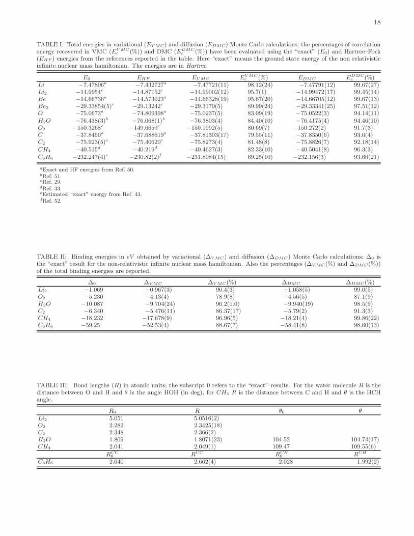
18

TABLE I: Total energies in variational (EV MC) and diffusion (EDMC) Monte Carlo calculations; the percentages of correlationenergy recovered in VMC (EV MC

c (%)) and DMC (EDMCc (%)) have been evaluated using the “exact” (E0) and Hartree–Fock

(EHF ) energies from the references reported in the table. Here “exact” means the ground state energy of the non relativisticinfinite nuclear mass hamiltonian. The energies are in Hartree.

E0 EHF EV MC EV MCc (%) EDMC EDMC

c (%)Li −7.47806a

−7.432727a−7.47721(11) 98.12(24) −7.47791(12) 99.67(27)

Li2 −14.9954c−14.87152c

−14.99002(12) 95.7(1) −14.99472(17) 99.45(14)Be −14.66736a

−14.573023a−14.66328(19) 95.67(20) −14.66705(12) 99.67(13)

Be2 −29.33854(5)c −29.13242c−29.3179(5) 89.99(24) −29.33341(25) 97.51(12)

O −75.0673a−74.809398a

−75.0237(5) 83.09(19) −75.0522(3) 94.14(11)H2O −76.438(3)b −76.068(1)b −76.3803(4) 84.40(10) −76.4175(4) 94.46(10)O2 −150.3268c

−149.6659c−150.1992(5) 80.69(7) −150.272(2) 91.7(3)

C −37.8450a−37.688619a

−37.81303(17) 79.55(11) −37.8350(6) 93.6(4)C2 −75.923(5)c −75.40620c

−75.8273(4) 81.48(8) −75.8826(7) 92.18(14)CH4 −40.515d

−40.219d−40.4627(3) 82.33(10) −40.5041(8) 96.3(3)

C6H6 −232.247(4)e −230.82(2)f −231.8084(15) 69.25(10) −232.156(3) 93.60(21)

aExact and HF energies from Ref. 50.bRef. 51.cRef. 29.dRef. 33.eEstimated “exact” energy from Ref. 43.fRef. 52.

TABLE II: Binding energies in eV obtained by variational (∆V MC) and diffusion (∆DMC) Monte Carlo calculations; ∆0 isthe “exact” result for the non-relativistic infinite nuclear mass hamiltonian. Also the percentages (∆V MC(%) and ∆DMC(%))of the total binding energies are reported.

∆0 ∆V MC ∆V MC(%) ∆DMC ∆DMC(%)Li2 −1.069 −0.967(3) 90.4(3) −1.058(5) 99.0(5)O2 −5.230 −4.13(4) 78.9(8) −4.56(5) 87.1(9)H2O −10.087 −9.704(24) 96.2(1.0) −9.940(19) 98.5(9)C2 −6.340 −5.476(11) 86.37(17) −5.79(2) 91.3(3)CH4 −18.232 −17.678(9) 96.96(5) −18.21(4) 99.86(22)C6H6 −59.25 −52.53(4) 88.67(7) −58.41(8) 98.60(13)

TABLE III: Bond lengths (R) in atomic units; the subscript 0 refers to the “exact” results. For the water molecule R is thedistance between O and H and θ is the angle HOH (in deg), for CH4 R is the distance between C and H and θ is the HCHangle.

R0 R θ0 θ

Li2 5.051 5.0516(2)O2 2.282 2.3425(18)C2 2.348 2.366(2)H2O 1.809 1.8071(23) 104.52 104.74(17)CH4 2.041 2.049(1) 109.47 109.55(6)

RCC0 RCC RCH

0 RCH

C6H6 2.640 2.662(4) 2.028 1.992(2)

19

TABLE IV: Binding energies in eV obtained by variational (∆V MC) and diffusion (∆DMC) Monte Carlo calculations withdifferent trial wave functions for benzene. In order to calculate the binding energies yielded by the 2-body Jastrow we usedthe atomic energies reported in Ref. 10. The percentages (∆V MC(%) and ∆DMC(%)) of the total binding energies are alsoreported.

∆V MC ∆V MC(%) ∆DMC ∆DMC(%)Kekule + 2body −30.57(5) 51.60(8) − −

resonating Kekule + 2body −32.78(5) 55.33(8) − −

resonating Dewar Kekule + 2body −34.75(5) 58.66(8) −56.84(11) 95.95(18)Kekule + 3body −49.20(4) 83.05(7) −55.54(10) 93.75(17)resonating Kekule + 3body −51.33(4) 86.65(7) −57.25(9) 96.64(15)resonating Dewar Kekule + 3body −52.53(4) 88.67(7) −58.41(8) 98.60(13)full resonating + 3body −52.65(4) 88.87(7) −58.30(8) 98.40(13)

TABLE V: Bond lengths (r) for the two lowest 2B2g and 2B3g states of the benzene radical cation. The angles α are expressedin degrees, the lengths in a0. The carbon sites are numerated from 1 to 6.

2B2g2B3g Computational method

acute obtuser(C1 − C2) 2.616 2.694 B3LYP/cc-pVTZ a

2.649 2.725 BLYP/6-31G* b

2.659(1) 2.733(4) SR-VMC c

r(C2 − C3) 2.735 2.579 B3LYP/cc-pVTZ a

2.766 2.615 BLYP/6-31G* b

2.764(2) 2.628(4) SR-VMC c

α(C6C1C2) 118.4 121.6 B3LYP/cc-pVTZ a

118.5 121.5 BLYP/6-31G* b

118.95(6) 121.29(17) SR-VMC c

aRef. 45bRef. 44cThis work

TABLE VI: Total energies for the 2B2g and 2B3g states of the benzene radical cation after the geometry relaxation. Acomparison with a BLYP/6-31G* and SVWN/6-31G* all-electron calculation (Ref. 44) is reported.

VMC DMC BLYP/6-31G* SVWN/6-31G*2B2g −231.4834(15) −231.816(3) −231.815495 −230.5479312B3g −231.4826(14) −231.812(3) −231.815538 −230.547751

TABLE VII: Adiabatic ionization potential of the benzene molecule; our estimate is done for the 2B3g relaxed geometries ofthe benzene radical cation, with an inclusion of the zero point motion correction between the 2B3g state and the 1A1g neutralmolecule ground state, calculated in Ref. 45 at the B3LYP/6-31G* level.

VMC a DMC a CCSD(T)/cc-pV∞Z b experiment c

AIP 8.86(6) 9.36(8) 9.29(4)∆ZPEad −0.074 −0.074 −0.074best estimate 8.79(6) 9.29(8) 9.22(4) 9.2437(8)

aThis workbRef. 45cRef. 53

20

TABLE VIII: Matrix of the λ coefficients of the geminal function expansion in the pairing determinant for the Li2 molecule.The matrix is symmetric to have a spin singlet, therefore we show only the upper part of it.

1sa 2sa 2pza 2pxa 2pya 3sa 1sb 2sb 2pzb 2pxb 2pyb 3sb

1sa 1 −2.162 10−3

−6.838 10−3

0 0 −2.877 10−3

0 0 0 0 0 0

2sa - 6.22 10−4

−1.601 10−4

0 0 2.031 10−3

0 6.79 10−3

−4.67 10−4

0 0 1.790 10−3

2pza - - −4.25 10−4

0 0 −1.132 10−3

0 −4.67 10−4

3.211 10−4

0 0 7.67 10−4

2pxa - - - −1.351 10−3

0 0 0 0 0 −1.173 10−3

0 0

2pya - - - - −1.351 10−3

0 0 0 0 0 −1.173 10−3

0

3sa - - - - - −1.541 10−3

0 1.790 10−3

7.67 10−4

0 0 −8.91 10−4

1sb - - - - - - 1 −2.162 10−3

−6.838 10−3

0 0 −2.877 10−3

2sb - - - - - - - 6.22 10−4

−1.601 10−4

0 0 1.790 10−3

2pzb - - - - - - - - −4.25 10−4

0 0 −1.132 10−3

2pxb - - - - - - - - - −1.351 10−3

0 0

2pyb - - - - - - - - - - −1.351 10−3

0

3sb - - - - - - - - - - - −1.541 10−3

TABLE IX: Matrix of the λ coefficients of the pairing function expansion in the three body Jastrow for the Li2 molecule. Asin the previous table only the upper part is reported .

sGa pGxa pGya pGza sGb pGxb pGyb pGzb

sGa −0.2427 0 0 −2.713 10−4−5.136 10−4 0 0 −1.202 10−5

pGxa - −0.1772 0 0 0 −7.997 10−3 0 0pGya - - −0.1772 0 0 0 −7.997 10−3 0pGza - - - 1.027 10−2 1.202 10−5 0 0 −8.749 10−3

sGb - - - - −0.2427 0 0 −2.713 10−4

pGxb - - - - - −0.1772 0 0pGyb - - - - - - −0.1772 0pGzb - - - - - - - 1.027 10−2

TABLE X: Orbital basis set parameters used for the Li2molecule. Since the molecule is homonuclear the parametersof the atom b are the same as the atom a.

z1 z2 p

φ1sa 2.4485 4.2891 0.4278φ2sa 0.5421 1.4143 −1.5500φ2pxa 0.6880 − −

φ2pya 0.6880 − −

φ2pza 1.0528 − −

φ3sa 0.6386 − −

φsGa 1.4356 − −0.2044φpGxa 0.7969 4.4217 −1.2689φpGya 0.7969 4.4217 −1.2689φpGza 8.980 10−3

−0.1924 0.3229