ECMOR XIII – 13th European Conference on the Mathematics of Oil Recovery Biarritz, France, 10-13 September 2012

A25Neural Networks and their Derivatives for HistoryMatching and other Seismic, Basin and ReservoirOptimization ProblemsJ. Bruyelle* (Terra 3E) & D.R. Guérillot (Terra 3E)

SUMMARYIn geosciences, complex forward problems met in geophysics, petroleum system analysis and reservoirengineering problems often requires replacing these forward problems by proxies, and these proxies areused for optimizations problems. For instance, History Matching of observed field data requires a so largenumber of reservoir simulation runs (especially when using geostatistical geological models) that it isoften impossible to use the full reservoir simulator. Therefore, several techniques have been proposed tomimic the reservoir simulations using proxies. Due to the use of experimental approach, most of authorspropose to use second order polynomials.

In this paper we demonstrate that:(1) Neural networks can also be second order polynomials. Therefore, the use of a neural network as aproxy is much more flexible and adaptable to the non linearity of the problem to be solved;(2) First order and second order derivatives of the neural network can be obtained providing gradients andhessian for optimizers.

For inverse problems met in seismic inversion, well by well production data, optimal well locations,source rock generation, etc., most of the time, gradient methods are used for finding an optimal solution.The paper will describe how to calculate these gradients from a neural network built as a proxy. Whenneeded, the hessian can also be obtained from the neural network approach.

On a real case study, the ability of neural networks to reproduce complex phenomena (water-cuts,production rates. etc.) is showed. Comparisons with second polynomials (and kriging methods) will bedone demonstrating the superiority of the neural network approach as soon as non linearity behaviors arepresent in the responses of the simulator. The gradients and the hessian of the neural network will becompared to those of the real response function.

Keywords: Proxies, History Matching, Gradient Methods, Optimizers, Basin Modelling, SeismicInversion, Uncertainty Analysis, Hessian.

ECMOR XIII – 13th

European Conference on the Mathematics of Oil Recovery

Biarritz, France, 10-13 September 2012

Introduction

Reservoir engineering procedures, such as history matching, production optimization (well placement,

production rate, etc.) or uncertainty analysis, require a large number of reservoirs simulation runs

which can result in a large computational effort. Quality of the results affects the estimations of

recoverable hydrocarbons. However, dealing with such problems can not only be done using a

simulator, as a reservoir simulation can last several hours. To bypass time consuming reservoir

simulations, some authors proposed to use proxies (Slotte et al. 2008; Amudo et al. 2009).

Several techniques such as polynomial approaches or kriging have been presented in the literature to

be used as proxies for reservoir simulators. In most cases, these used proxies are not suited to real

problems because they are not adapted to represent nonlinear phenomena.

The proxy model presented in this paper uses artificial neural networks, an approach gaining rapidly

acceptance in fields requiring tremendous computer power (aerospace-flight simulation, defense-

missile guidance, or security-face recognition) and which is particularly well suited to reproduce non

linearities. It has been also used for reservoirs simulations (Silva et al. 2007; Costa et al. 2010).

When using optimization algorithms, it could important to get the first and, eventually second,

derivatives, if one would like to solve an optimization problem. Therefore, three questions interest us

here:

(1) Does neural network approximate as well as second order polynomials?

(2) Is it possible to obtain the first and second derivatives of the neural network approaching

the reservoir simulator?

(3) Are these derivatives of the neural network good approximations of the derivatives of the

simulator?

In this paper, after recalling briefly the concept and design of a neural network, advantages of using

neural networks as proxy, we show that:

(1) Neural networks can perfectly reproduce second order polynomials therefore they are

more general;

(2) First and second order derivatives of neural networks can be obtained in the same

“learning” process than the proxy itself;

(3) The first derivatives of the neural network are good approximates of the derivatives of the

simulator at least in the case but it was not the case for the second derivatives.

To illustrate the advantages of neural networks, a comparison of different proxies reproducing bottom

hole pressure, water-cut and gas-oil ratio on a synthetic model is made. This synthetic model, named

PUNQ-S3, is inspired by an actual field which was operated by Elf Exploration Production. Then, the

first and second order derivative neural network of the objective function for a history matching

problem will be given and compared to the gradient computed from real simulations.

Artificial neural network topology

The artificial neurons are based on the same architecture as those of biological neurons. An artificial

neuron is connected to one or more inputs, processes the information collected via an activation

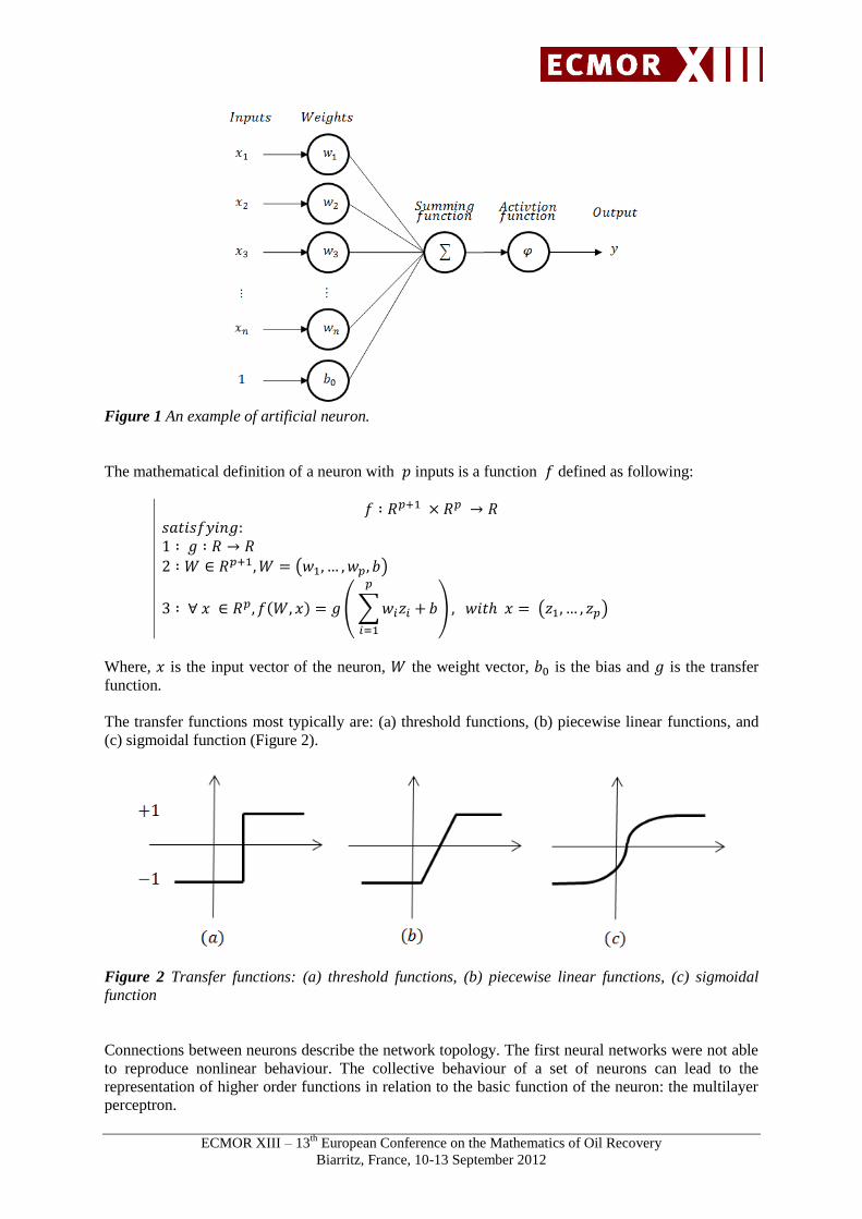
function, and passes the results to other neurons. Figure 1 shows an example of artificial neuron.

Each neuron is an elementary process. A neuron receives a number of inputs from other neurons. For

each of these inputs, a weight is assigned to give it more or less importance. Each neuron has only one

output that will feed the inputs of other neurons.

ECMOR XIII – 13th

European Conference on the Mathematics of Oil Recovery

Biarritz, France, 10-13 September 2012

Figure 1 An example of artificial neuron.

The mathematical definition of a neuron with inputs is a function defined as following:

Where, is the input vector of the neuron, the weight vector, is the bias and is the transfer

function.

The transfer functions most typically are: (a) threshold functions, (b) piecewise linear functions, and

(c) sigmoidal function (Figure 2).

Figure 2 Transfer functions: (a) threshold functions, (b) piecewise linear functions, (c) sigmoidal

function

Connections between neurons describe the network topology. The first neural networks were not able

to reproduce nonlinear behaviour. The collective behaviour of a set of neurons can lead to the

representation of higher order functions in relation to the basic function of the neuron: the multilayer

perceptron.

ECMOR XIII – 13th

European Conference on the Mathematics of Oil Recovery

Biarritz, France, 10-13 September 2012

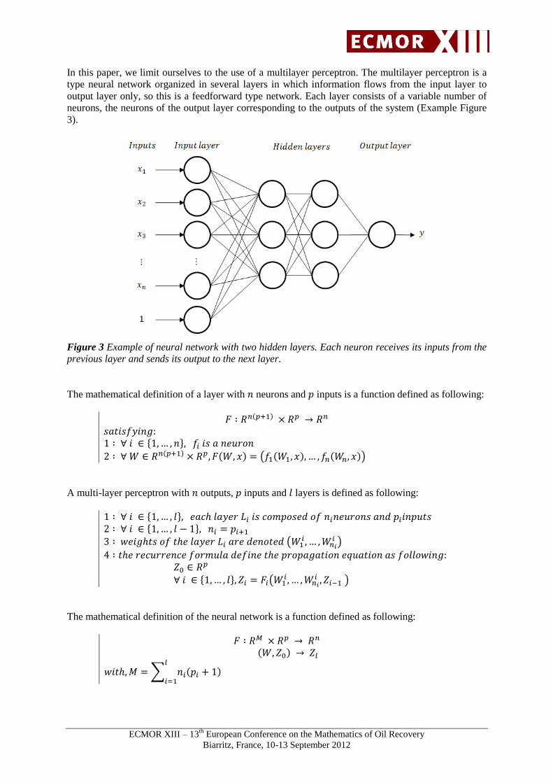
In this paper, we limit ourselves to the use of a multilayer perceptron. The multilayer perceptron is a

type neural network organized in several layers in which information flows from the input layer to

output layer only, so this is a feedforward type network. Each layer consists of a variable number of

neurons, the neurons of the output layer corresponding to the outputs of the system (Example Figure

3).

Figure 3 Example of neural network with two hidden layers. Each neuron receives its inputs from the

previous layer and sends its output to the next layer.

The mathematical definition of a layer with neurons and inputs is a function defined as following:

A multi-layer perceptron with outputs, inputs and layers is defined as following:

The mathematical definition of the neural network is a function defined as following:

ECMOR XIII – 13th

European Conference on the Mathematics of Oil Recovery

Biarritz, France, 10-13 September 2012

The mechanism to calculate the outputs of a neural network is called the propagation and is defined as

follows:

A remarkable property of a neural network is its learning ability, i.e. to reproduce a function from a

set of learning points. Indeed, the coupling to a neural network with a learning algorithm can

reproduce complex physical phenomena. The first neural networks were not able to reproduce

nonlinear problems; this limitation was removed through the backpropagation (Werbos 1974;

Rumelhart et al. 1986) of the gradient of the error in multilayer systems. The learning algorithm

consists to adjust the weights (or parameters) of the network. To do this, examples of the problem to

reproduce are shown to the neural network; the error between the desired outputs and the observed

outputs is calculated. This error is backward through the network from the output layer towards the

input layer.

Neural network as universal approximation

The advantage of perceptron neural networks is explained by the following result (Cybenko 1988 and

1989; Hornik et al. 1989 and 1990; Hornik 1991): neural networks with one hidden layer can

approach, with the desired accuracy, any continuous function (or even other functions that are not

necessarily continuous): this is what we call the universal approximation capability and this is also

what allows them to be applied very effectively to many models.

Universal approximation theorem(Cybenko 1989): An arbitrary continuous

function, defined on [0,1] can be arbitrary well uniformly approximated by a

multilayer feed-forward neural network with one hidden layer (that contains

only finite number of neurons) using neurons with arbitrary activation functions

in the hidden layer and a linear neuron in the output layer.

ECMOR XIII – 13th

European Conference on the Mathematics of Oil Recovery

Biarritz, France, 10-13 September 2012

Let be the arbitrary activation5 function. Then, f C([0,1]), > 0: n

N, wi, ai, bi R, i{0… n}:

as an approximation of the function f(.); that is

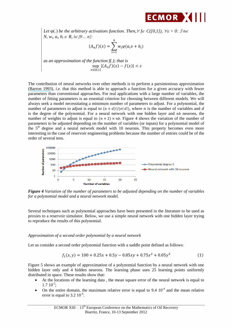
The contribution of neural networks over other methods is to perform a parsimonious approximation

(Barron 1993), i.e. that this method is able to approach a function for a given accuracy with fewer

parameters than conventional approaches. For real applications with a large number of variables, the

number of fitting parameters is an essential criterion for choosing between different models. We will

always seek a model necessitating a minimum number of parameters to adjust. For a polynomial, the

number of parameters to adjust is equal to , where is the number of variables and

is the degree of the polynomial. For a neural network with one hidden layer and neurons, the

number of weights to adjust is equal to . Figure 4 shows the variation of the number of

parameters to be adjusted depending on the number of variables (or inputs) for a polynomial model of

the 5th degree and a neural network model with 10 neurons. This property becomes even more

interesting in the case of reservoir engineering problems because the number of entries could be of the

order of several tens.

Figure 4 Variation of the number of parameters to be adjusted depending on the number of variables

for a polynomial model and a neural network model.

Several techniques such as polynomial approaches have been presented in the literature to be used as

proxies to a reservoir simulator. Below, we use a simple neural network with one hidden layer trying

to reproduce the results of this polynomial.

Approximation of a second order polynomial by a neural network

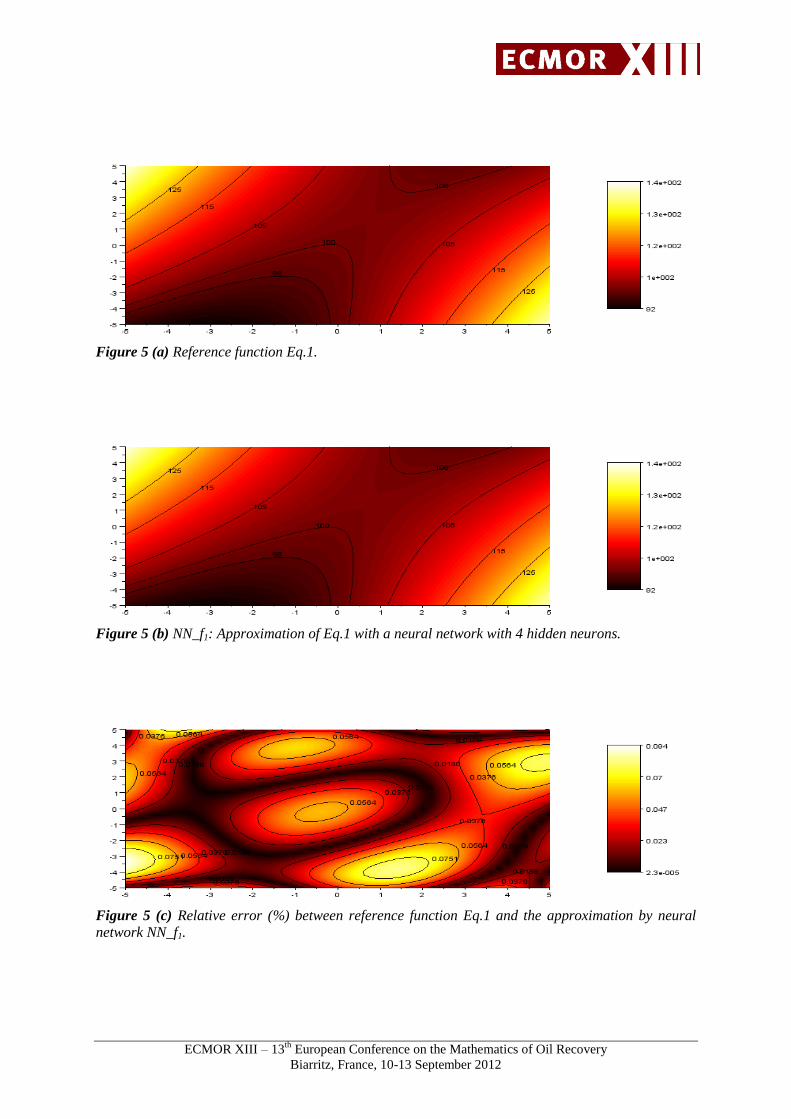
Let us consider a second order polynomial function with a saddle point defined as follows:

Figure 5 shows an example of approximation of a polynomial function by a neural network with one

hidden layer only and 4 hidden neurons. The learning phase uses 25 learning points uniformly

distributed in space. These results show that:

At the locations of the learning data , the mean square error of the neural network is equal to

1.7 10-3

;

On the entire domain, the maximum relative error is equal to 9.4 10-4

and the mean relative

error is equal to 3.2 10-4

.

ECMOR XIII – 13th

European Conference on the Mathematics of Oil Recovery

Biarritz, France, 10-13 September 2012

Figure 5 (a) Reference function Eq.1.

Figure 5 (b) NN_f1: Approximation of Eq.1 with a neural network with 4 hidden neurons.

Figure 5 (c) Relative error (%) between reference function Eq.1 and the approximation by neural

network NN_f1.

ECMOR XIII – 13th

European Conference on the Mathematics of Oil Recovery

Biarritz, France, 10-13 September 2012

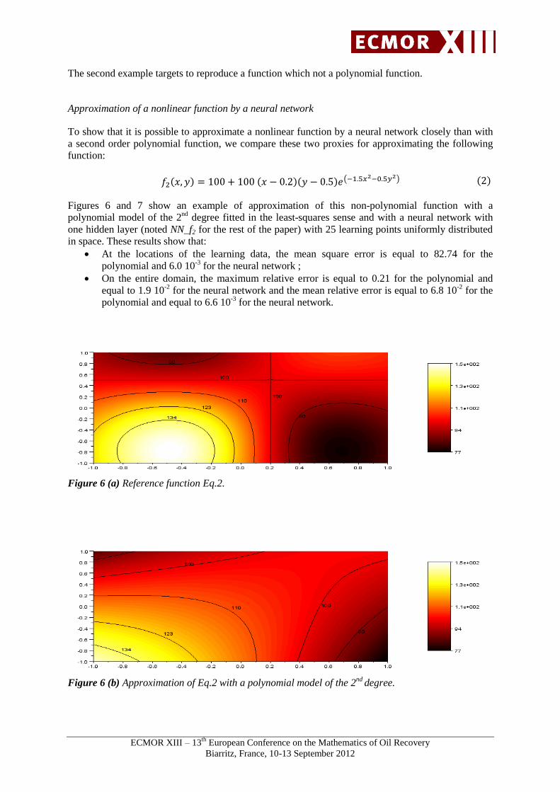
The second example targets to reproduce a function which not a polynomial function.

Approximation of a nonlinear function by a neural network

To show that it is possible to approximate a nonlinear function by a neural network closely than with

a second order polynomial function, we compare these two proxies for approximating the following

function:

Figures 6 and 7 show an example of approximation of this non-polynomial function with a

polynomial model of the 2nd

degree fitted in the least-squares sense and with a neural network with

one hidden layer (noted NN_f2 for the rest of the paper) with 25 learning points uniformly distributed

in space. These results show that:

At the locations of the learning data, the mean square error is equal to 82.74 for the

polynomial and 6.0 10-3

for the neural network ;

On the entire domain, the maximum relative error is equal to 0.21 for the polynomial and

equal to 1.9 10-2

for the neural network and the mean relative error is equal to 6.8 10-2

for the

polynomial and equal to 6.6 10-3

for the neural network.

Figure 6 (a) Reference function Eq.2.

Figure 6 (b) Approximation of Eq.2 with a polynomial model of the 2nd

degree.

ECMOR XIII – 13th

European Conference on the Mathematics of Oil Recovery

Biarritz, France, 10-13 September 2012

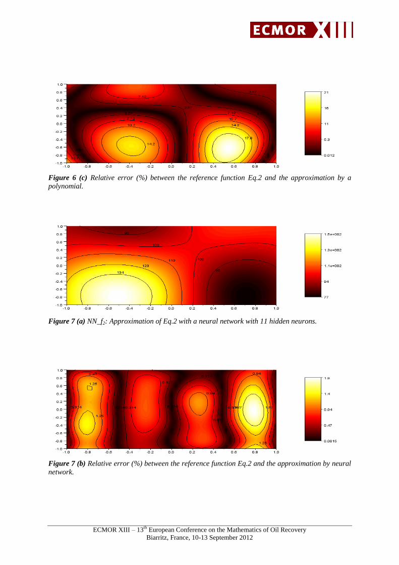
Figure 6 (c) Relative error (%) between the reference function Eq.2 and the approximation by a

polynomial.

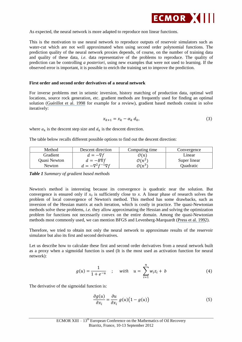
Figure 7 (a) NN_f2: Approximation of Eq.2 with a neural network with 11 hidden neurons.

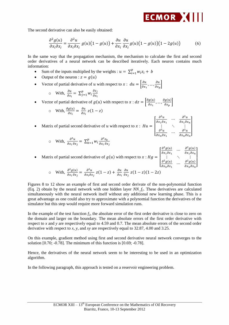
Figure 7 (b) Relative error (%) between the reference function Eq.2 and the approximation by neural

network.

ECMOR XIII – 13th

European Conference on the Mathematics of Oil Recovery

Biarritz, France, 10-13 September 2012

As expected, the neural network is more adapted to reproduce non linear functions.

This is the motivation to use neural network to reproduce outputs of reservoir simulators such as

water-cut which are not well approximated when using second order polynomial functions. The

prediction quality of the neural network proxies depends, of course, on the number of training data

and quality of these data, i.e. data representative of the problems to reproduce. The quality of

prediction can be controlling a posteriori, using new examples that were not used to learning. If the

observed error is important, it is possible to enrich the training set to improve the prediction.

First order and second order derivatives of a neural network

For inverse problems met in seismic inversion, history matching of production data, optimal well

locations, source rock generation, etc. gradient methods are frequently used for finding an optimal

solution (Guérillot et al. 1998 for example for a review), gradient based methods consist in solve

iteratively:

,

where is the descent step size and is the descent direction.

The table below recalls different possible options to find out the descent direction:

Method Descent direction Computing time Convergence

Gradient Linear

Quasi Newton Super linear

Newton Quadratic

Table 1 Summary of gradient based methods

Newton's method is interesting because its convergence is quadratic near the solution. But

convergence is ensured only if x0 is sufficiently close to x. A linear phase of research solves the

problem of local convergence of Newton's method. This method has some drawbacks, such as

inversion of the Hessian matrix at each iteration, which is costly in practice. The quasi-Newtonian

methods solve these problems, i.e. they allow approximating the Hessian and solving the optimization

problem for functions not necessarily convex on the entire domain. Among the quasi-Newtonian

methods most commonly used, we can mention BFGS and Levenberg-Marquardt (Press et al. 1992).

Therefore, we tried to obtain not only the neural network to approximate results of the reservoir

simulator but also its first and second derivatives.

Let us describe how to calculate these first and second order derivatives from a neural network built

as a proxy when a sigmoidal function is used (It is the most used as activation function for neural

network):

The derivative of the sigmoidal function is:

ECMOR XIII – 13th

European Conference on the Mathematics of Oil Recovery

Biarritz, France, 10-13 September 2012

The second derivative can also be easily obtained:

In the same way that the propagation mechanism, the mechanism to calculate the first and second

order derivatives of a neural network can be described iteratively. Each neuron contains much

information:

Sum of the inputs multiplied by the weights :

Output of the neuron :

Vector of partial derivative of with respect to :

o With,

Vector of partial derivative of with respect to :

o With,

Matrix of partial second derivative of with respect to :

o With,

Matrix of partial second derivative of with respect to :

o With,

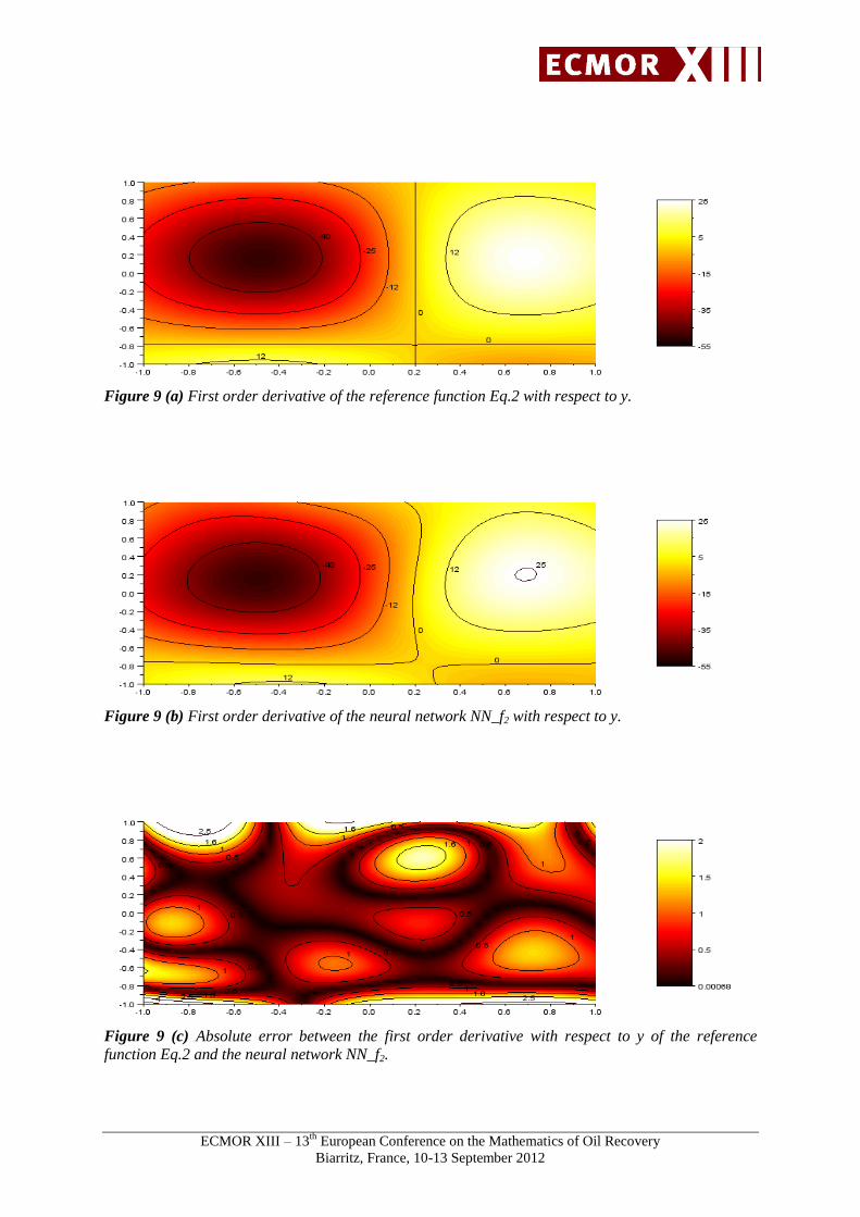
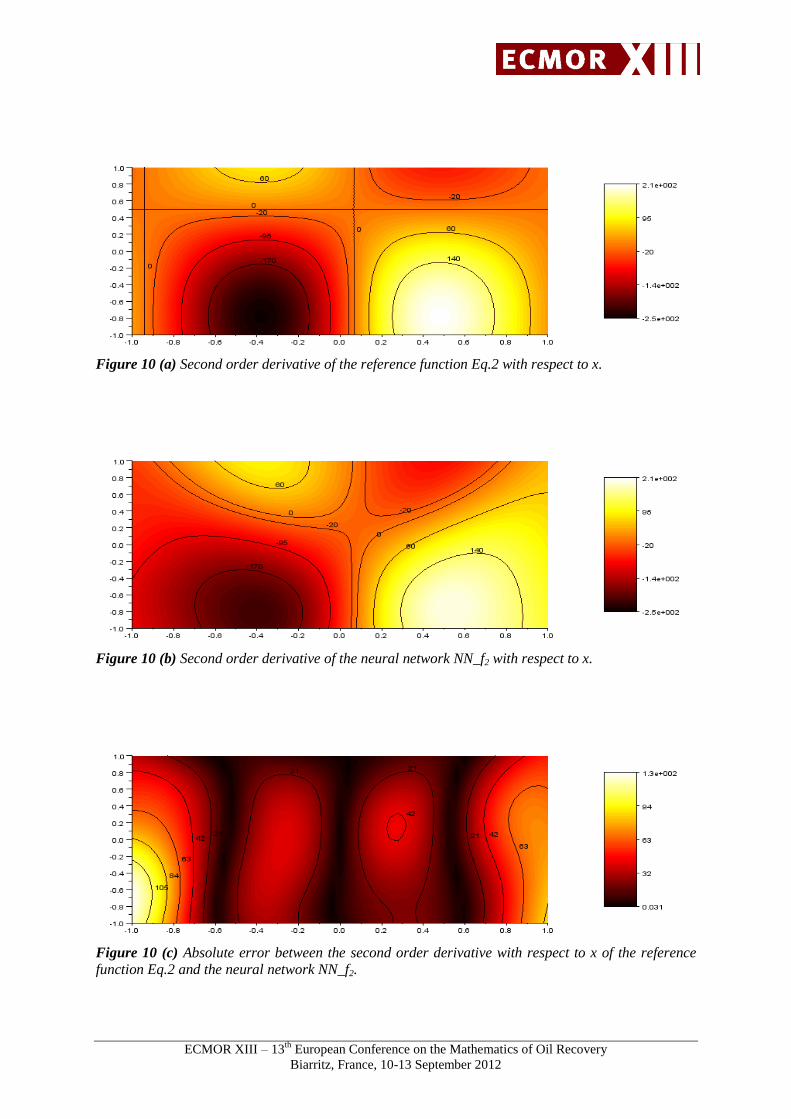
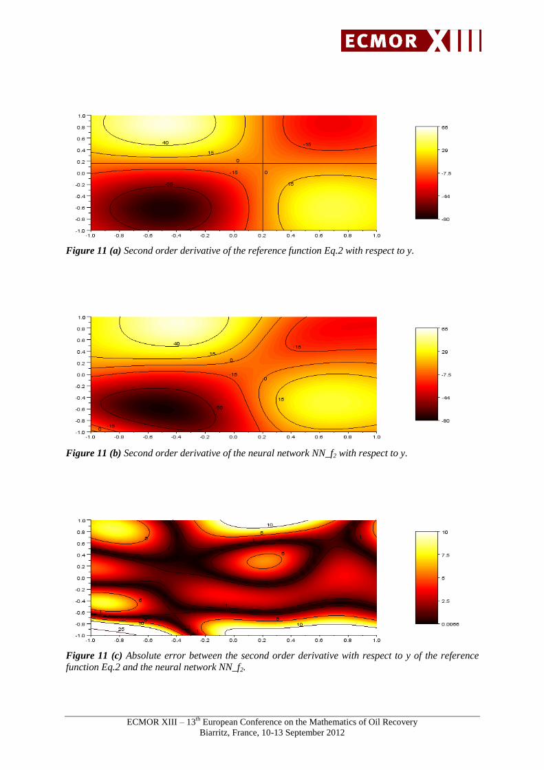
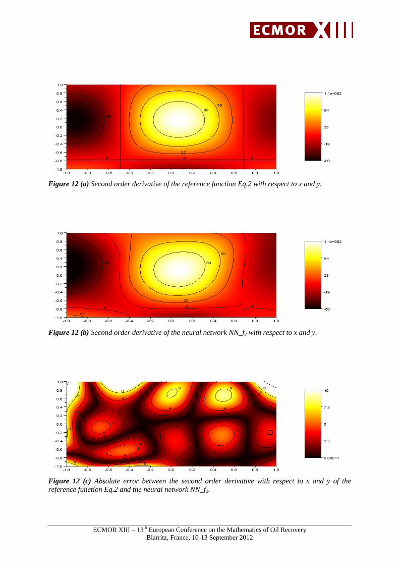
Figures 8 to 12 show an example of first and second order derivate of the non-polynomial function

(Eq. 2) obtain by the neural network with one hidden layer NN_f2. These derivatives are calculated

simultaneously with the neural network itself without any additional new learning phase. This is a

great advantage as one could also try to approximate with a polynomial function the derivatives of the

simulator but this step would require more forward simulation runs.

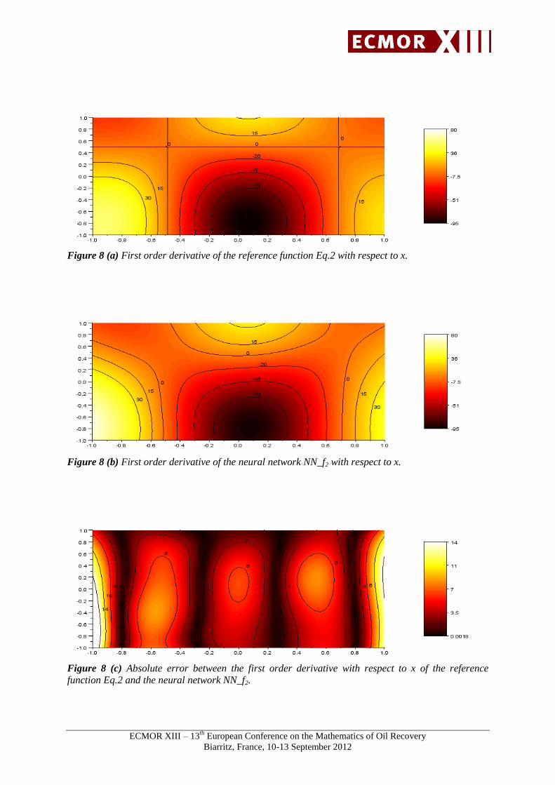
In the example of the test function f2, the absolute error of the first order derivative is close to zero on

the domain and larger on the boundary. The mean absolute errors of the first order derivative with

respect to x and y are respectively equal to 4.59 and 0.7. The mean absolute errors of the second order

derivative with respect to x, y, and xy are respectively equal to 32.87, 4.00 and 3.25.

On this example, gradient method using first and second derivative neural network converges to the

solution [0.70; -0.78]. The minimum of this function is [0.69; -0.78].

Hence, the derivatives of the neural network seem to be interesting to be used in an optimization

algorithm.

In the following paragraph, this approach is tested on a reservoir engineering problem.

ECMOR XIII – 13th

European Conference on the Mathematics of Oil Recovery

Biarritz, France, 10-13 September 2012

Figure 8 (a) First order derivative of the reference function Eq.2 with respect to x.

Figure 8 (b) First order derivative of the neural network NN_f2 with respect to x.

Figure 8 (c) Absolute error between the first order derivative with respect to x of the reference

function Eq.2 and the neural network NN_f2.

ECMOR XIII – 13th

European Conference on the Mathematics of Oil Recovery

Biarritz, France, 10-13 September 2012

Figure 9 (a) First order derivative of the reference function Eq.2 with respect to y.

Figure 9 (b) First order derivative of the neural network NN_f2 with respect to y.

Figure 9 (c) Absolute error between the first order derivative with respect to y of the reference

function Eq.2 and the neural network NN_f2.

ECMOR XIII – 13th

European Conference on the Mathematics of Oil Recovery

Biarritz, France, 10-13 September 2012

Figure 10 (a) Second order derivative of the reference function Eq.2 with respect to x.

Figure 10 (b) Second order derivative of the neural network NN_f2 with respect to x.

Figure 10 (c) Absolute error between the second order derivative with respect to x of the reference

function Eq.2 and the neural network NN_f2.

ECMOR XIII – 13th

European Conference on the Mathematics of Oil Recovery

Biarritz, France, 10-13 September 2012

Figure 11 (a) Second order derivative of the reference function Eq.2 with respect to y.

Figure 11 (b) Second order derivative of the neural network NN_f2 with respect to y.

Figure 11 (c) Absolute error between the second order derivative with respect to y of the reference

function Eq.2 and the neural network NN_f2.

ECMOR XIII – 13th

European Conference on the Mathematics of Oil Recovery

Biarritz, France, 10-13 September 2012

Figure 12 (a) Second order derivative of the reference function Eq.2 with respect to x and y.

Figure 12 (b) Second order derivative of the neural network NN_f2 with respect to x and y.

Figure 12 (c) Absolute error between the second order derivative with respect to x and y of the

reference function Eq.2 and the neural network NN_f2.

ECMOR XIII – 13th

European Conference on the Mathematics of Oil Recovery

Biarritz, France, 10-13 September 2012

Applications on PUNQ-S3 reservoir

The case study used to illustrate the advantages of neural network modeling for various reservoir

engineering problems is the PUNQ-S3 reservoir. We are going first to use a neural network as a

proxy, than its derivatives for an optimization problem.

The case study

This test case was widely presented and studied in the literature (Gu and Oliver 2004; Hajizadeh et al.

2010). This is a synthetic model of a real field which was operated by Elf Exploration Production.

The field contains six production wells located around the gas-oil contact. The production scheduling

has been inspired by the original model: a first year of extended well testing, followed by a three year

shut-in period prior to field production. To collect well test data, the first two weeks of each year are

used for each well to do a build-up test (cf. Figure 14). Each well operates under production

constraint. After falling below a limiting bottom hole pressure, wells will switch to BHP-constraint.

The PUNQ-S3 model is composed of 5 layers. The model contains 19x28x5 grid blocks, of which

1761 blocks are active.

Figure 13 PUNQ-S3 model with wells positions.

Figure 14 Oil production rate for each well.

ECMOR XIII – 13th

European Conference on the Mathematics of Oil Recovery

Biarritz, France, 10-13 September 2012

The uncertain geological parameters of PUNQ-S3 are the porosities, the vertical and horizontal

permeabilities. The parameterization of PUNQ-S3 model is based on the geological description. We

consider each facies, as describe in the geological description, and the 18 parameters are the

homogeneous porosities and the homogeneous vertical and horizontal permeabilities of each of 6

facies.

The history matching problem consists to fit production data. The production data used to defined the

objective function are: bottom hole pressure, gas-oil ratio and water-cut.

The objective function is defined as follows:

Where, is the number of wells, is the number of production data type for the well and is

the number of production data report times for the well and the production data type . For a parameter sample , observed data

are compared with simulated data at time step

with a measure error and a weight .

After performing a sensitivity analysis to quantify the impact of the 18 parameters on the objective

function, we have selected the 11 most influential parameters.

Comparison of different proxies to reproduce bottom hole pressure, water-cut and gas-oil ratio

Three proxies are compared: 1) polynomial model, 2) Bayesian model and 3) the neural network.

These comparisons are done on their ability to reproduce three different results of the simulator: the

bottom hole pressure, the water cut and the gas-oil ratio. A first set of forward simulations were used

either to find out the three proxies. Then, these three proxies were compared on a second set

composed of three simulations which were not part of the first set.

The first set is composed of 102 simulations: the 44 simulations used for the sensitivity analysis (the 4

equal spacing samples of the 11 most influential parameters), plus the 33 simulations performed using

an experimental design approach with the 11 most influential parameters, and 25 others selected

randomly.

The polynomial model of second order (quadratic model) is determined by a least-square fit between

the polynomial response and the results of the set 1.

Universal kriging proxy (Aanonsen et al. 1995; Pan and Horne 1998) assumes that the true model

follows a Gaussian process with a pre-specified correlation function and an unknown variance

determined by maximizing the outcome likelihood.

Neural network proxy is composed of one hidden layer with 10 neurons.

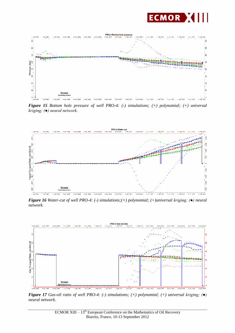
Figure 15 to 17 show results for the well PRO-4. The results of these proxies are compared to the

simulation results of the set 2. For these three results (blue, green and red line), neural network

reproduces perfectly the bottom hole pressure, the water-cut and the gas-oil ratio.

The two other proxies do not fit as well the results of the set 2.

ECMOR XIII – 13th

European Conference on the Mathematics of Oil Recovery

Biarritz, France, 10-13 September 2012

Figure 15 Bottom hole pressure of well PRO-4: (-) simulations; (×) polynomial; (+) universal

kriging; (●) neural network.

Figure 16 Water-cut of well PRO-4: (-) simulations;(×) polynomial; (+)universal kriging; (●) neural

network.

Figure 17 Gas-oil ratio of well PRO-4: (-) simulations; (×) polynomial; (+) universal kriging; (●)

neural network.

ECMOR XIII – 13th

European Conference on the Mathematics of Oil Recovery

Biarritz, France, 10-13 September 2012

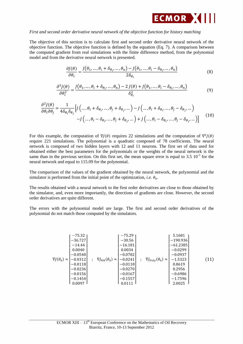
First and second order derivative neural network of the objective function for history matching

The objective of this section is to calculate first and second order derivative neural network of the

objective function. The objective function is defined by the equation (Eq. 7). A comparison between

the computed gradient from real simulations with the finite difference method, from the polynomial

model and from the derivative neural network is presented.

For this example, the computation of requires 22 simulations and the computation of

require 221 simulations. The polynomial is a quadratic composed of 78 coefficients. The neural

network is composed of two hidden layers with 12 and 11 neurons. The first set of data used for

obtained either the best parameters for the polynomials or the weights of the neural network is the

same than in the previous section. On this first set, the mean square error is equal to 3.5 10-5

for the

neural network and equal to 115.09 for the polynomial.

The comparison of the values of the gradient obtained by the neural network, the polynomial and the

simulator is performed from the initial point of the optimization, i.e. .

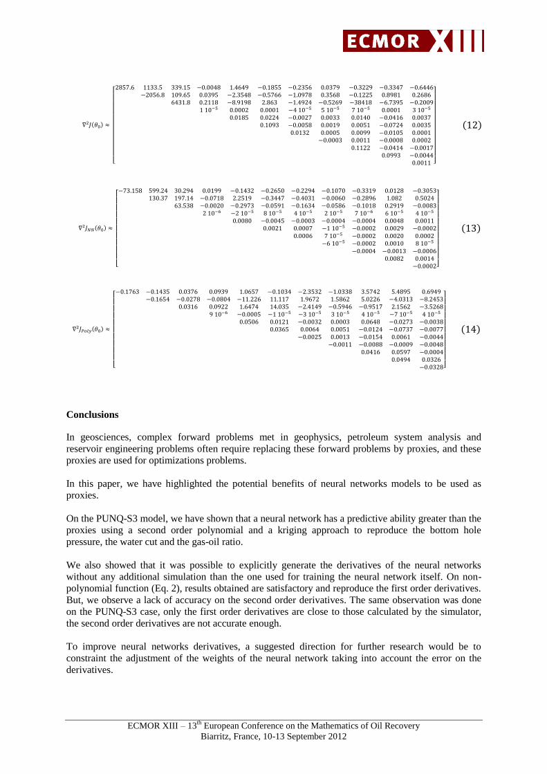
The results obtained with a neural network to the first order derivatives are close to those obtained by

the simulator, and, even more importantly, the directions of gradients are close. However, the second

order derivatives are quite different.

The errors with the polynomial model are large. The first and second order derivatives of the

polynomial do not match those computed by the simulators.

ECMOR XIII – 13th

European Conference on the Mathematics of Oil Recovery

Biarritz, France, 10-13 September 2012

Conclusions

In geosciences, complex forward problems met in geophysics, petroleum system analysis and

reservoir engineering problems often require replacing these forward problems by proxies, and these

proxies are used for optimizations problems.

In this paper, we have highlighted the potential benefits of neural networks models to be used as

proxies.

On the PUNQ-S3 model, we have shown that a neural network has a predictive ability greater than the

proxies using a second order polynomial and a kriging approach to reproduce the bottom hole

pressure, the water cut and the gas-oil ratio.

We also showed that it was possible to explicitly generate the derivatives of the neural networks

without any additional simulation than the one used for training the neural network itself. On non-

polynomial function (Eq. 2), results obtained are satisfactory and reproduce the first order derivatives.

But, we observe a lack of accuracy on the second order derivatives. The same observation was done

on the PUNQ-S3 case, only the first order derivatives are close to those calculated by the simulator,

the second order derivatives are not accurate enough.

To improve neural networks derivatives, a suggested direction for further research would be to

constraint the adjustment of the weights of the neural network taking into account the error on the

derivatives.

ECMOR XIII – 13th

European Conference on the Mathematics of Oil Recovery

Biarritz, France, 10-13 September 2012

References

Aanonsen, S.I., Eide, A.L., Holden, L., Aasen, J.O. [1995] Optimizing Reservoir Performance Under

Uncertainty with Application to Well Location. SPE 30710, SPE Annual Technical Conference and

Exhibition, held in Dallas, USA, 22-25 October 1995.

Amudo, C., Graf, T., Dandekar, R. and Randle, J. [2009] The Pains and Gains of Experimental

Design and Response Surface Applications in Reservoir Simulation Studies. SPE 118709, SPE

Reservoir Simulation Symposium held in The Woodlands, Texas, USA.

Barron, A. [1993] Universal approximation bounds for superposition of a sigmoidal function, IEEE

Transactions on Information Theory, 39, p. 930-945.

Costa, L.A.N, Maschio, C. and Schiozer, D.J. [2010] Study of the Influence of Training Data Set in

Artificial Neural Network Applied to the History Matching Process, Rio Oil & Gas Expo and

Conference, 13-16 September, Rio de Janeiro, Brazil.

Cybenko, G. [1988] Continuous Valued Neural Networks with Two Hidden Layers are Sufficient.

Technical Report, Department of Computer Science, Tufts University.

Cybenko, G. [1989] Approximation by Superpositions of Sigmoidal Functions. Mathematics of

Control, Signals, and Systems.

Gu, Y. and Oliver, D.S. [2004] History Matching of the PUNQ-S3 Reservoir Model Using the

Ensemble Kalman Filter, SPE 89942, SPE Annual Technical Conference held in Houston, Texas,

U.S.A. 26-29 september 2004.

Guérillot, D., Lazaar, S. and Pianelo, L. [1998] Inverse Methods in Geoscience Modelling: a Review

for Prospective. 6th European Conference on the Mathematics of Oil Recovery, Peebles, Sept. 8-11,

Proc., Paper C-33, p. 8.

Hajizadeh, Y., Christie, M. and Demyanov, V. [2010] Comparative Study of Novel Population-based

Optimization Algorithms for History Matching and Uncertainty Quantification: PUNQ-S3 Revisited,

SPE 136861, ADIPEC Conference, Abu Dhabi, United Arab Emirates, 1-4 November 2010.

Hornik, K., Stinchcombe, M. and White, H. [1989] Multilayer Feedforward Networks are Universal

Approximators, Neural Networks, 2, p. 359-366.

Hornik, K., Stinchcombe, M. and White, H. [1990] Universal Approximation of an Unknown

Mapping and its Derivatives Using Multilayer Feedforward Networks, Neural Networks, 3, p. 551-

560.

Hornik, K. [1991] Approximation Capabilities of Multilayer Feedforward Networks, Neural

Networks, 4, p. 251-257.

Pan, Y. and Horne, R.N. [1998] Improved Methods for Multivariate Optimization of Field

Development Scheduling and Well Placement Design. SPE 49055, SPE Annual Technical Conference

and Exhibition held in New Orleans, Louisiana, 27-30 September 1998.

Press, W. H., Teukolsky, S. A., Vetterling, W. T. and Flannery, B. P. [1992] Numerical Recipes in C:

The Art of Scientific Computing (second edition), Cambridge University Press.

Rumelhart, D. E., Hinton, G. E. and Williams, R. J. [1986] Learning Internal Representations by Error

Backpropagation, Parallel Distributed Processing: Explorations in the Microstructure of Cognition,

p. 318- 362, MIT Press.

ECMOR XIII – 13th

European Conference on the Mathematics of Oil Recovery

Biarritz, France, 10-13 September 2012

Silva, P.C., Maschio, C. and Schiozer, D.J. [2007] Use of Neuro-Simulation techniques as proxies to

reservoir simulator: Application in production history matching, Journal of Petroleum Science and

Engineering, Vol. 57, pp. 273-280.

Slotte, P.A. and Smorgrav, E. [2008] Response Surface Methodology Approach for History Matching

and Uncertainty Assessment of Reservoir Simulation Models, SPE 113390, SPE EUROPEC/EAGE

Annual Conference and Exhibition held in Rome, Italy, 9-12 June 2008.

Werbos, P. J. [1974] Beyond Regression: New Tools for Prediction and Analysis in the Behavioral

Sciences, Ph. D. thesis, Harvard University.