Remote Sensing of Environment 115 (2011) 3615–3624

Contents lists available at SciVerse ScienceDirect

Remote Sensing of Environment

j ourna l homepage: www.e lsev ie r .com/ locate / rse

NDVI responses to the forest canopy and floor from spring to summer observed byairborne spectrometer in eastern Siberia

Rikie Suzuki a,⁎, Hideki Kobayashi a, Nicolas Delbart b,a, Jun Asanuma c, Tetsuya Hiyama d

a Research Institute for Global Change, Japan Agency for Marine-Earth Science and Technology, 3173-25 Showa-machi, Kanazawa-ku, Yokohama, Kanagawa 236-0001, Japanb Université Paris Diderot (Paris 7), PRODIG (UMR 8586), Paris, Francec Terrestrial Environment Research Center, University of Tsukuba, Tennodai, Tsukuba, Ibaraki 305-8577, Japand Research Institute for Humanity and Nature, 457-4 Motoyama, Kamigamo, Kita-ku, Kyoto 603-8047, Japan

⁎ Corresponding author. Tel.: +81 45 778 5541.E-mail address: rikie@jamstec.go.jp (R. Suzuki).

0034-4257/$ – see front matter © 2011 Elsevier Inc. Alldoi:10.1016/j.rse.2011.08.022

a b s t r a c t

a r t i c l e i n f o

Article history:Received 31 August 2007Received in revised form 17 July 2011Accepted 27 August 2011Available online 28 September 2011

Keywords:Boreal forestForest radiative transfer modelForest understorySpectral reflectanceTaigaTree crown

A popular method of satellite-based monitoring of the photosynthetic potential of vegetation is to calculatethe normalised difference vegetation index (NDVI) from measurements of the red (RED) and near-infrared(NIR) bands. Enormous amounts of vegetation information have been obtained over continental to globalareas based on NDVI derived from NOAA-AVHRR, Terra/Aqua-MODIS, and SPOT-VEGETATION satellite obser-vations. In eastern Siberia, where sparse boreal forests are dominant, the lack of landscape-scale canopy-reflectance observations impedes interpretation of how NDVI seasonality is controlled by the forest canopyand floor status. We discuss the NDVI of the canopy and floor separately based on airborne spectral reflec-tance measurements and simultaneous airborne land surface images acquired around Yakutsk, Siberia,using a hedgehopping aircraft from spring to summer 2000. The aerial land surface images (4402 scenes)were visually classified into four types according to the forest condition: no-green canopy and snow floor(Type 1), green canopy and snow floor (Type 2), no-green canopy and no-snow floor (Type 3), and greencanopy and no-snow floor (Type 4). The spectral reflectance from 350 to 1200 nm was then calculated forthese four types. Type 1 had almost no difference in reflectance between the RED and NIR bands, and the re-sultant NDVI was slightly negative (−0.03). Although Type 2 showed a significant difference between thetwo bands because of canopy greenness, the resultant NDVI was rather low (0.17) because of high reflectionfrom the snow cover on the floor. In Type 3, the significant difference between the two bands was mainlycaused by the greenness of the floor, and the NDVI was relatively high (0.45). The NDVI for Type 4 was thehighest (0.75) among the four types. The contributions of reflectance from the forest canopy and floor tothe total reflectance were tested with a forest radiative transfer model. The reflectance difference betweenNIR and RED bands (NIR−RED) of Type 4 (15.6%) was approximately double the differences of Type 2(7.0%) and of Type 3 (7.9%), suggesting half-and-half contributions of forest canopy greenness and floorgreenness to the total greenness. The result also suggested that the satellite-derived NDVI in the larch forestaround Yakutsk reaches 85% of the maximum NDVI owing to the forest floor greenness, and only the other15% of the increase in NDVI should be attributed to the canopy foliation. These results quantitatively revealthat the NDVI depends considerably on forest floor greenness and snow cover in addition to canopy green-ness in the case of relatively sparse forest in Siberia.

rights reserved.

© 2011 Elsevier Inc. All rights reserved.

1. Introduction

A vegetation index calculated from the difference in spectral re-flectance between the red (RED) and near-infrared (NIR) bands is acommon method of monitoring the photosynthetic potential of vege-tation on the land surface using remotely sensed data (e.g., Tucker,1979). The best-known index is the normalised difference vegetation

index (NDVI), computed as NDVI=(NIR−RED)/(NIR+RED) (e.g.,Tarpley et al., 1984), from radiometric measurements by sensorssuch as the Advanced Very High Resolution Radiometer (AVHRR) ofNOAA, the Moderate-resolution Imaging Spectroradiometer (MODIS)of Terra/Aqua, the VEGETATION (VGT) sensor of SPOT, or the En-hanced Thematic Mapper Plus (ETM+) of Landsat.

NDVI has been used in numerous studies on the spatio-temporalcharacteristics of vegetation at continental to global scales. Such stud-ies have revealed, for example, trends in NDVI and vegetation produc-tivity in response to climatic factors (e.g., Nemani et al., 2003, Piaoet al., 2011, Tucker et al., 2001). Using NDVI, Dye and Tucker (2003)discussed the trends and seasonality of vegetation productivity and

3616 R. Suzuki et al. / Remote Sensing of Environment 115 (2011) 3615–3624

snow-cover, in relation to temperature in northern Eurasia. Studieshave also investigated the relationship between vegetation distribu-tion and meteorology (e.g., Suzuki et al., 2006), between vegetationproductivity and atmospheric circulation patterns (Buermann et al.,2003; Vicente-Serrano et al., 2006), between interannual vegetationchanges and atmospheric CO2 content (Kondoh et al. (2002)), and be-tween interannual changes in vegetation and actual evapotranspira-tion (Suzuki et al., 2007).

The NDVI has also been used to estimate the global leaf area index(LAI), which represents the one-sided leaf area per unit of groundarea (e.g., Asrar et al., 1984; Myneni et al., 1997; Sellers et al.,1996). However, especially in sparse forests such as the Siberiantaiga, those satellite sensors measure the total greenness of the forestcanopy as well as viewable parts of the forest floor, as previouslystressed by Eriksson et al. (2006) and Rautiainen (2005). Consequent-ly, the LAI estimated using such an NDVI would involve mixed infor-mation for both the forest canopy and forest floor. For practicalapplications, the Climate and Vegetation Research Group of BostonUniversity has developed and distributed a global LAI product(MOD15) constructed from MODIS measurements. Although the in-verse model for LAI estimation was rigorously designed (Knyazikhinet al., 1999; Myneni et al. 2002), the separation of the forest canopyand floor is rather ambiguous in the forest biome category.

Eriksson et al. (2006) demonstrated that the forest understory hada major impact on LAI estimation from satellite measurements oversouthern Sweden. Peddle et al. (2001, 1999) developed a spectralmixture analysis and optical reflectance model for boreal forest con-sidering the influence from the background (forest floor and under-story). Kobayashi et al. (2007), on the basis of radiative transfermodel results, also emphasised that forest floor conditions affect thereflectance in the NIR band even if the canopy leaf area conditiondoes not change. These previous studies indicate that the forestfloor plays an important role in forest remote sensing, especially inestimating the LAI.

Although previous studies estimated the behaviour of the spectralreflectance of forests, which consist of canopy and understory (orfloor), by mathematical analyses and numerical models, understand-ing and knowledge of the canopies and floors of actual forests has

Fig. 1. The land surface around Yakutsk observed using Landsat ETM+ (19 June 2000), andshow the flight plan described in the text and Table 2. The symbols “S” and “U” indicate the

been insufficient. In particular, studies based on measurements of ac-tual forest canopy and floor that can be related to remote sensing areneeded. Pisek and Chen (2009), for example, in a study on back-ground reflectivity using Multi-angle Imaging Spectro Radiometer(MISR) data over North America, stated that information on theforest background (i.e., forest floor) helps to improve LAI estimation.McCallum et al. (2010) emphasised a real need for more in situ mea-surements of vegetation over northern Eurasia for validating the fractionof absorbed photosynthetically active radiation (FAPAR) estimated bysatellite remote sensing.

Our purpose was to determine the roles of forest canopy green-ness and forest floor greenness in NDVIs. For this purpose, we usedan original methodology based on aircraft radiometric measurementsof actual forests over a 100-km-wide region of eastern Siberia, and onforest radiative transfer simulations. The study data set consisted ofaircraft observations taken over 7 days from spring to summer 2000around Yakutsk in eastern Siberia (Hiyama et al., 2003). Using avideo camera and spectrometer onboard the hedgehopping aircraft,we obtained thousands of visual images of the forests and simulta-neous spectral reflectance measurements from the snow season tosummer. Snow cover masked the forest floor in spring, and conse-quently, the spectral characteristic of only the canopy emerged.Meanwhile, data obtained when the canopy was leafless but nosnow covered the floor in deciduous forests enabled us to examinethe forest floor NDVI. We also simulated the spectral reflectance ofthe forest canopy and floor using a radiative transfer model and in-vestigated the significance of the forest floor to remotely sensedobservations.

2. Aircraft and satellite data

2.1. Aircraft-based land surface data

Apart from the Antarctic continent, the area (Fig. 1) of aircraft ob-servation in this study has the coldest recorded winter climate in theworld. The mean air temperature at Yakutsk in July is about 18 °C,with temperatures dropping to approximately −40 °C in January.Snow covers the land surface from October to early May, and

the flight course used for aircraft-based observations. L1 to L8, R1 to R8, and T1 and T2locations of the surface stations at Spasskaya Pad and Ulakhan Sykkhan, respectively.

3617R. Suzuki et al. / Remote Sensing of Environment 115 (2011) 3615–3624

continuous permafrost prevails. The Lena River flows from south tonorth through the middle of the study area. A flat low riverine plainmostly covered by grassland vegetation borders the Lena River. Tothe west and east of this riverine lowland, the left and right bank ter-races of the Lena River spread extensively. These terraces are approx-imately 100 m higher than the riverine lowland (about 200 m abovemean sea level), and the relief is relatively uniform. The land coverof the terraces is characterised by taiga forest, in which thedominant tree species is larch (Larix gmelinii, deciduous) (Shulze etal., 1995) with some pine (Pinus sylvestris, evergreen) and birch(Betula platyphylla, deciduous) (Japan National Committee for GAMEand GAME-Siberia Subcommittee, 2001). The mean tree stand heightand tree stand density measured at Spasskaya Pad (62°15′18″N,129°37′08″E), a surface site in a larch forest of the study area, were18 m and 840 trees ha−1, respectively (Ohta et al., 2001).

The spatial proportions of larch, birch, and pine forest are about60%, 10%, and 7% over the terrace regions, respectively (Suzuki etal., 2004). Various kinds of willow and fir occur at some sites, butthese sites occur relatively infrequently. Cowberry (Vacciniumvitis-idaea, evergreen), a typical plant in Siberian larch forests, isthe major forest floor species. This plant has little clear seasonality,so forest floor conditions are almost unchangeable during periods ofno snow (Kobayashi et al., 2007).

Generally, the snow cover in the observation area melts complete-ly by early May. Deciduous larch trees begin to foliate at the end ofMay and reach the mature stage in June. To cover these seasonalchanges in the land surface and vegetation, aircraft observationswere carried out on 9 days over the period from April to June 2000;this study used data from 7 of these 9 days (Table 1). Hiyama et al.(2003) have provided details of the aircraft-based observations.

All flights on the seven days followed a fixed course and schedule(Fig. 1 and Table 2). The flight course consisted of three components:grid-runs over the left (L1–L8) and right (R1–R8) terraces and atransverse run (T1–T2). The west–east length of each leg in thegrid-run was 36 km, and the north–south interval of the grid was4 km on both terraces. The transverse run was 90 km in length. Theflight altitudes, 100 m and 150 m, were measured above the highestpoint of the terrace.

A Russian Ilyushin-18 aircraft was used for the observations. Theaircraft was equipped with a video movie camera (VMC) and a spec-trometer. The VMC was a typical home-use video camera (DCR-TRV900, Sony, NTSC), with a field of view (FOV) of 61.8° horizontally,48.3° vertically, and 73.6° diagonally. The VMC was tightly fixed onthe floor of the aircraft in a vertical position directed toward theground through an observation window. Land surface images fromthe nadir angle were recorded during the flight legs.

A spectrometer (FieldSpec FR, Analytical Spectral Devices, USA)was installed in the aircraft with the terminal of the optical fibre(light collector) tightly fixed perpendicular to the aircraft floor and

Table 1Timing of aircraft-based observations, and the number of scenes sampled from video imagesof the larch forest. General characteristics of forest canopy and floor for those days are give

Date ofobservation

Season Number ofscenes

Forest visual characteristics

Canopy

24 April Pre-snowmelt 610 No green leaves on deciduous trees, gre1 May Snow melt 673 No green leaves on deciduous trees, gre12 May Pre-foliation 616 No green leaves on deciduous trees, gre20 May Pre-foliation,

foliating629 Mostly no green leaves on deciduous tre

trees5 June Foliated 605 Green leaves on nearly all the trees

9 June Foliated 631 Green leaves on nearly all the trees

19 June Foliated 638 Green leaves on nearly all the trees

Total – 4402

directed downward to view the surface from the nadir angle throughthe same observation window as used for the VMC. The FOV of thelight collector was 25°, which was roughly equivalent to circles withdiameters of 44 m and 67 m at flight altitudes of 100 m and 150 m,respectively. The spectrometer measured radiances from the landsurface at spectral wavelengths from 350 to 2500 nm at 1-nm inter-vals. Measurements had a mean duration of 1 s and occurred every10 s.

To derive the reflectance of the land surface, spectral observationsof global solar radiation were made using the other FieldSpec FR spec-trometer at the following surface sites: Spasskaya Pad on April 24,May 1, 12, 20, and June 19, 2000; and the rooftop of a building inYakutsk city on June 5 and 9, 2000 (Fig. 1). Reflected radiance froma white reference board exposed to global solar radiation was mea-sured at 1-min intervals during the aircraft flights at these surfacesites. Ideally, spectral observation of the global solar radiation shouldbe conducted on the aircraft together with spectral observation of theland surface. However, it was technically impossible to find a positionon the aircraft where the global solar radiation was measurable by thespectrometer.

The two FieldSpec FR spectrometers were mutually calibratedbased on simultaneous measurements of the same white referenceboard at Spasskaya Pad, and the reflectance was calculated as theratio of airborne radiance to white reference board radiance. Basical-ly, the nearest timing combination of the 1-s interval measurement ofthe airborne spectrometer and the 1-min interval measurement ofthe surface sites spectrometer was used for that ratio calculation. Al-though the positions of the flying aircraft and the two surface siteswere some distance apart, we considered this acceptable for the re-flectance calculation because the solar illumination was homogenouson the 7 observation days (all fine weather); cases in which the solarradiation was interrupted by cloud were excluded from the analysis.

No atmospheric correction was applied to the spectral data becausethe flight altitudes (basically 100 and 150 m) were low enough to notrequire such correction. The spectral reflectance data set is availableon a CD-ROM and on the Internet (Suzuki et al., 2003a; http://w3.jamstec.go.jp/iorgc/hcorp/data/database/cdc/siberia/sub4.html).

2.2. SPOT VGT S10 data

The result based on aircraft-based data is discussed in relation tosatellite-based vegetation data over an extensive area of Siberia. Asthe satellite-based vegetation data, SPOT-VGT, a representative dataset that is often used for vegetation behaviour analyses over extensive(continental to global) areas, was employed. The SPOT-VGT data usedwere 10-day-composite data (S10) with a resolution of 1/112°(~0.5×1 km at Yakutsk (60°N)) in the Plate Carrée geographic pro-jection for year 2000, available at http://free.vgt.vito.be/. The NDVI isderived from the red (610–680 nm) and near-infrared (780–

. Pre-foliation, foliating, and foliated seasons were discriminated based on the conditionn briefly.

Floor

en leaves on evergreen (pine) trees Almost covered by snowen leaves on evergreen (pine) trees Mostly covered by snowen leaves on evergreen (pine) trees No snow, patchily covered by green vegetationes, green leaves on evergreen (pine) No snow, patchily covered by green

vegetationNo snow, patchily covered by greenvegetationNo snow, patchily covered by greenvegetationNo snow, patchily covered by greenvegetation

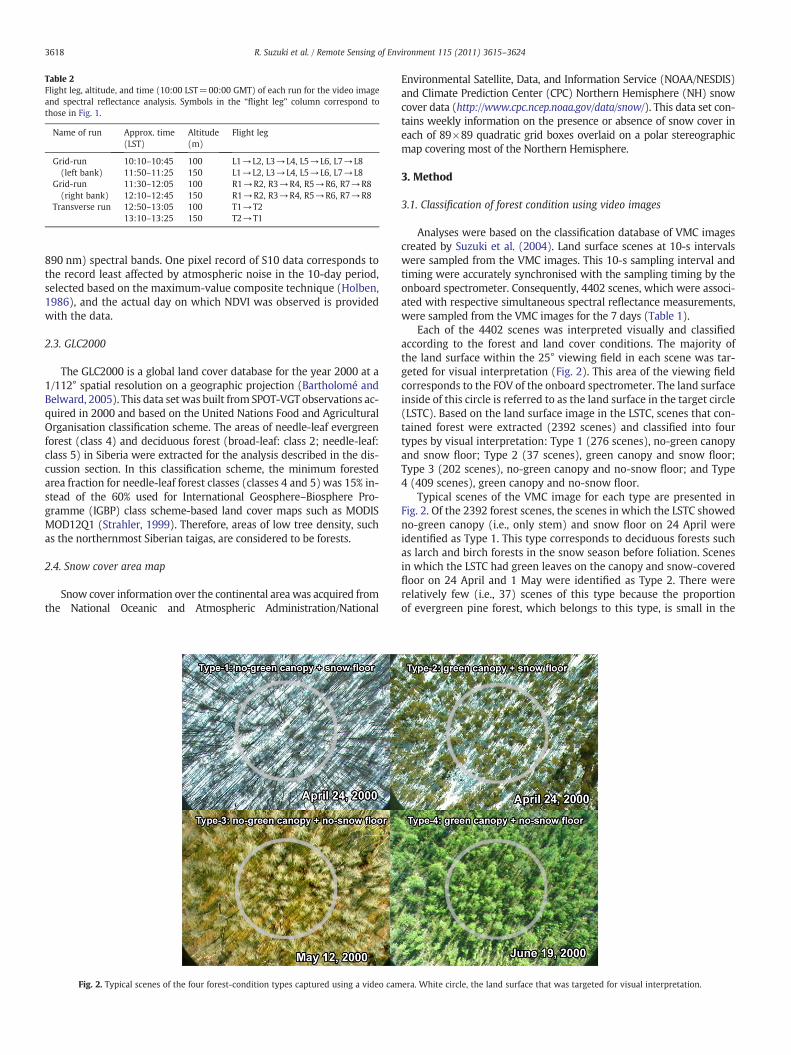
Table 2Flight leg, altitude, and time (10:00 LST=00:00 GMT) of each run for the video imageand spectral reflectance analysis. Symbols in the “flight leg” column correspond tothose in Fig. 1.

Name of run Approx. time(LST)

Altitude(m)

Flight leg

Grid-run(left bank)

10:10–10:45 100 L1→L2, L3→L4, L5→L6, L7→L811:50–11:25 150 L1→L2, L3→L4, L5→L6, L7→L8

Grid-run(right bank)

11:30–12:05 100 R1→R2, R3→R4, R5→R6, R7→R812:10–12:45 150 R1→R2, R3→R4, R5→R6, R7→R8

Transverse run 12:50–13:05 100 T1→T213:10–13:25 150 T2→T1

3618 R. Suzuki et al. / Remote Sensing of Environment 115 (2011) 3615–3624

890 nm) spectral bands. One pixel record of S10 data corresponds tothe record least affected by atmospheric noise in the 10-day period,selected based on the maximum-value composite technique (Holben,1986), and the actual day on which NDVI was observed is providedwith the data.

2.3. GLC2000

The GLC2000 is a global land cover database for the year 2000 at a1/112° spatial resolution on a geographic projection (Bartholomé andBelward, 2005). This data set was built from SPOT-VGT observations ac-quired in 2000 and based on the United Nations Food and AgriculturalOrganisation classification scheme. The areas of needle-leaf evergreenforest (class 4) and deciduous forest (broad-leaf: class 2; needle-leaf:class 5) in Siberia were extracted for the analysis described in the dis-cussion section. In this classification scheme, the minimum forestedarea fraction for needle-leaf forest classes (classes 4 and 5) was 15% in-stead of the 60% used for International Geosphere–Biosphere Pro-gramme (IGBP) class scheme-based land cover maps such as MODISMOD12Q1 (Strahler, 1999). Therefore, areas of low tree density, suchas the northernmost Siberian taigas, are considered to be forests.

2.4. Snow cover area map

Snow cover information over the continental area was acquired fromthe National Oceanic and Atmospheric Administration/National

Fig. 2. Typical scenes of the four forest-condition types captured using a video cam

Environmental Satellite, Data, and Information Service (NOAA/NESDIS)and Climate Prediction Center (CPC) Northern Hemisphere (NH) snowcover data (http://www.cpc.ncep.noaa.gov/data/snow/). This data set con-tains weekly information on the presence or absence of snow cover ineach of 89×89 quadratic grid boxes overlaid on a polar stereographicmap covering most of the Northern Hemisphere.

3. Method

3.1. Classification of forest condition using video images

Analyses were based on the classification database of VMC imagescreated by Suzuki et al. (2004). Land surface scenes at 10-s intervalswere sampled from the VMC images. This 10-s sampling interval andtiming were accurately synchronised with the sampling timing by theonboard spectrometer. Consequently, 4402 scenes, which were associ-ated with respective simultaneous spectral reflectance measurements,were sampled from the VMC images for the 7 days (Table 1).

Each of the 4402 scenes was interpreted visually and classifiedaccording to the forest and land cover conditions. The majority ofthe land surface within the 25° viewing field in each scene was tar-geted for visual interpretation (Fig. 2). This area of the viewing fieldcorresponds to the FOV of the onboard spectrometer. The land surfaceinside of this circle is referred to as the land surface in the target circle(LSTC). Based on the land surface image in the LSTC, scenes that con-tained forest were extracted (2392 scenes) and classified into fourtypes by visual interpretation: Type 1 (276 scenes), no-green canopyand snow floor; Type 2 (37 scenes), green canopy and snow floor;Type 3 (202 scenes), no-green canopy and no-snow floor; and Type4 (409 scenes), green canopy and no-snow floor.

Typical scenes of the VMC image for each type are presented inFig. 2. Of the 2392 forest scenes, the scenes in which the LSTC showedno-green canopy (i.e., only stem) and snow floor on 24 April wereidentified as Type 1. This type corresponds to deciduous forests suchas larch and birch forests in the snow season before foliation. Scenesin which the LSTC had green leaves on the canopy and snow-coveredfloor on 24 April and 1 May were identified as Type 2. There wererelatively few (i.e., 37) scenes of this type because the proportionof evergreen pine forest, which belongs to this type, is small in the

era. White circle, the land surface that was targeted for visual interpretation.

Table 3Optical parameters in the red and near-infrared regions for the radiative transfer modelFLiES.

Species Optical parameters Near-infrared (%) Red (%)

Larcha Needle reflectance 47.0 7.8Needle transmittance 37.0 5.8Stem reflectance 32.0 15.0

Pineb Needle reflectance 51.0 5.0Needle transmittance 11.0 1.0Stem reflectance 34.0 25.0

Vaccinium vitis-idaeac Reflectance 41.3 4.9Soila Reflectance 12.0 6.0Snow Reflectance 46.6 56.1

a Kobayashi et al. (2007).b Nilson and Peterson (1991).c Kushida et al. (2007).

3619R. Suzuki et al. / Remote Sensing of Environment 115 (2011) 3615–3624

study region (7% of the total, as mentioned above). Type 3 was identi-fied as no-green canopy (i.e., only stem) and no-snow floor on 12 and20 May. According to the ground-based forest survey in 2000, these2 days fell between the end of snow melt and the start of foliationfor most larch and birch trees. Deciduous forest such as larch andbirch forests belong to Type 3 in this period. The forest floor of Type3 showed various kinds of condition, such as evergreen plants (mostcases), bare ground, fallen trees and leaves, burned floor after forestfire, and rarely water. Although we could not analyse the floor condi-tion because of the low resolution of the VMC and blurred images dueto the aircraft movement, the major effect of the greenness of ever-green plants appeared in the no-snow floor condition. For Type 4,the LSTC showed green canopy and no-snow floor in June. Both decid-uous and evergreen forests in the foliated season belong to this type.Although the floor was not viewable in some cases of Type 4 due tothe dense forest canopy, we can regard it as no-snow floor becauseType 4 only included images for days in June when snow coverwould not exist anywhere in the study area.

In most scenes, the LSTC was a uniform patch of land cover. LSTCsthat included two types of land cover were excluded from the ana-lyses. No LSTC clearly contained more than two types of land cover.In addition to these forest scenes, scenes that had only snow cover(e.g., frozen lake and river surfaces on 24 April and 1 May) werealso sampled (126 scenes) as references for the spectral reflectancefrom the snow surface.

In the targeted forest scenes (2392 scenes), tree stand density ran-ged from approximately 350 to 3200 trees ha−1. Tree stand densitywas roughly estimated by counting the number of tree stands in sev-eral representative forest scenes in which the actual size of a land sur-face object, such as tire tracks made by a car, could be identified forestimating the geographic scale of the scene. The examples of fourforests presented in Fig. 2 are relatively dense. The tree stand densitymay exceed 3200 trees ha−1 when dwarf trees that are unidentifiablein VMC images are included.

3.2. Forest radiative transfer model (FLiES)

To examine the reflectance variations in the RED and NIR bandsfor the four forest-condition types, we conducted a radiative transfersimulation using a three-dimensional (3-D) canopy radiative transfermodel (Forest Light Environmental Simulator [FLiES]; Kobayashi andIwabuchi, 2008; Kobayashi et al., 2007). The model uses a Monte-Carlo-based photon tracing technique for bi-directional reflectancesampling. The reliability was confirmed by the RAdiationModel Inter-comparison (RAMI) exercise online checker (ROMC) (Widlowski etal., 2008). The accuracy was checked by comparison with severalROMC reference datasets complied from simulated results of sixexisting 3-D radiative transfer models. The model discernibility(Pinty et al., 2001) for the simulated bidirectional reflectance factorfrom FLiES was less than 3% compared with the ROMC referencedatasets.

In this study, we simulate the reflectance from two tree species(larch and pine) under various tree densities and forest floor condi-tions representing the forest around the Yakutsk area. To performthe reflectance simulation, the FLiES model requires informationsuch as individual tree sizes and positions in the forest canopy to con-figure the simulation. The forest configuration was generated fromforest census data sets (Yabuki, Ishii, and Tanaka, personal communi-cation) for the larch forest at Ulakhan Sykkhan, Siberia (Fig. 1). Thetree density at that site was 2822 trees ha−1 for canopy heightN5 m. The LAI value for the foliated (green) canopy was estimatedas 0.88 based on the field measurement by the fish-eye camera(Suzuki et al., 2001a). In addition to this original forest configuration,we prepared another four forest configurations with different treestand densities (i.e. the total was five densities) for the four forest-condition types, 20%, 50%, 80%, 100%, and 110% of the original tree

density at Ulakhan Sykkhan, by randomly removing or adding trees.This variation in tree density approximately corresponds to the treedensity variation observed in the VMC images, i.e., 350–3200 treesha−1. The canopy LAIs of all Type 2 and Type 4 forests were set at0.16, 0.41, 0.70, 0.87, and 0.93 for 20%, 50%, 80%, 100%, and 110%tree densities, respectively. The canopy LAIs of Type 1 and Type 3 for-ests were set to 0.

The optical parameters of the larch forest elements and the soilsurface in the simulation were cited from Kobayashi et al. (2007)and other literature and are given in Table 3 for the RED and NIRbands of MODIS (bands 1 and 2). MODIS is a widely used satellite sen-sor for the monitoring of land surface conditions. The snow reflec-tance was calculated by averaging the spectral reflectance of theaforementioned 126 snow surface scenes. As larch forest occupies84% of all forests in this area (Suzuki et al., 2004), we applied the op-tical parameters of the larch forest for the simulation of Type 1, Type3, and Type 4. Because Type 2 corresponds to only pine forest (i.e., ev-ergreen forest), we applied the optical parameters of pine forest forthe Type 2 simulation.

For Type 1 and Type 2 simulations we used 100% snow-coveredfloor conditions and performed five simulations by varying the fivetree stand densities. For Type 3 and Type 4 simulations, the forestfloor was visually indistinct in VMC images due to the foliated canopyand stem of the stands. Therefore, the forest floor condition was as-sumed to be a linear mixture of V. vitis-idaea in two cases; 100% soilfloor and 59% soil plus 41% V. vitis-idaea floor. The proportion, 59%soil and 41% V. vitis-idaea, was the value based on the field measure-ment at a larch forest site near Spasskaya Pad according to Kushida etal. (2007). We performed 10 simulations with variations of the fivetree densities and the two floor conditions.

Solar zenith angles were set at 55.59° for Type 1 and Type 2, 45.95°for Type 3, and 40.18° for Type 4, which were chosen as values closeto the actual airborne observation geometries (these changed withthe observation date). The observation angle was set at nadir.

4. Results

4.1. Spectral reflectance dependency on forest canopy and floor conditions

The mean spectral reflectance of Type 1 to Type 4 and the snowsurface from 350 to 1200 nm was calculated (Fig. 3) by averagingall the samples of each type and the snow surface. As a whole, thespectral reflectance of snow was relatively low compared to idealisticsnow surface reflectance because the targeted snowpack was ob-served just before the snow melt and its reflectivity had considerablydecreased due to impurities. Type 1, which had no green on the forestcanopy and floor, showed only the spectral characteristics of thesnow, i.e., high reflectance in the visible band and low reflectance in

0

20

40

60

80

100

refle

ctan

ce (

%)

400 600 800 1000 1200wave length (nm)

snow (# scene = 126)Type-1: no-green canopy + snow floor (# scene = 276)Type-2: green canopy + snow floor (# scene = 37)Type-3: no-green canopy + no-snow floor (# scene = 202)Type-4: green canopy + no-snow floor (# scene = 409)

Fig. 3. Mean spectral reflectances of the four forest-condition types and snow surface.The standard deviation is denoted by vertical bars for each type and snow surface. 0

20

40

60

refle

ctan

ce in

nea

r-in

frar

ed b

and

(%)

0 20 40 60 80

reflectance in red band (%)

ND

VI

= 0

.8N

DV

I =

0.6

ND

VI =

0.4

ND

VI =

0.2

NDVI = 0.

0

NDVI = -0

.2

snow

Type-1: no-green canopy + snow floor

Type-2: green canopy + snow floor

Type-3: no-green canopy + no-snow floor

Type-4: green canopy + no-snow floor

Fig. 4. Reflectance in the red and near-infrared bands observed using the airborne spec-trometer. The four forest-condition types and snow surface are indicated by the respec-tive symbols. The NDVI contours are denoted by straight lines.

Table 4Mean reflectance (%) in the red (RED) and near-infrared (NIR) bands (equivalent tothose of MODIS) and the mean NDVI for each forest-condition type and snow surfaceaccording to the airborne spectrometer measurement.

Type No. ofscenes

NIR RED NIR−RED NDVI

Snow 126 46.6 56.1 −9.5 −0.091: No-green canopy+snow floor 276 22.6 24.0 −1.4 −0.032: Green canopy+snow floor 37 25.1 18.1 7.0 0.173: No-green canopy+no-snow floor 202 12.7 4.8 7.9 0.454: Green canopy+no-snow floor 409 18.2 2.6 15.6 0.75

3620 R. Suzuki et al. / Remote Sensing of Environment 115 (2011) 3615–3624

the near-infrared band. However, the total reflectance was lower thanthat of snow because of the presence of trees stems and theirshadows. The importance of tree stand shadows to the forest totalspectral reflectance was pointed out by Peddle et al. (1999) basedon a spectral mixture analysis. In Type 2, canopy greenness resultedin a significant reflectance difference around 700 nm, which sepa-rates the RED and NIR bands. However, the total reflectance of Type2 was high because of reflection from the snow on the floor. Type 3had no green in the forest canopy, but exposed green vegetation onthe floor. This condition led to a large difference in the spectral reflec-tance curve around 700 nm. The magnitude of the difference wassimilar to that of Type 2, but the total reflectance was lower than inType 2 because there was no snow cover to elevate the reflectancecurve. In Type 4, a very high reflectance difference, about double thedifferences of Type 2 and Type 3, was found around 700 nm becauseof the green canopy and green floor. The reflectance of Type 4, thefully foliated condition, was relatively low, i.e., 18.2% and 2.6% inNIR and RED bands, respectively. Similar low reflectance, around17% and 3% in NIR and RED bands, respectively, was also reportedby O'Neill et al. (1997), who measured the reflectance of a boreal for-est in Canada using an airborne spectrometer. The contribution of re-flectance from non-photosynthetic endmembers (tree stems, barefloor, litter) of the forest to the total reflectance is considered to behigh because of the sparseness of the tree stand.

4.2. NDVI dependency on forest canopy and floor conditions

NDVIs were calculated for the four forest-condition types based onthe aircraft observation. The mean reflectance in the RED (620–670 nm) and NIR (841–876 nm) wavelength bands (the same bandsas for MODIS) observed by FieldSpec FRs was used for the NDVI calcu-lation. Fig. 4 illustrates the relationship between reflectance in REDand NIR bands for each case of four types and the snow surface. Themean reflectance values in the two bands, NIR–RED, and the meanNDVI for the four types and snow surface are summarised inTable 4. The differences among the mean NDVIs of the types wereall significant at the 99% level (both sides) according to t-tests.

The snow showed high reflectance both in the RED and NIR bands,whereas the NDVI of snow was slightly negative (mean NDVI of−0.09) because the NIR reflectance was lower than the RED reflec-tance. Scattering of the plotted points appeared due to variation ofthe snow purity. Reflectance values for Type 1 (no-green canopy+snow floor) were distributed along the same line as the snow surfacevalues (Fig. 4), but both RED and NIR reflectance values were lowerthan those for the snow surface. The NDVI of Type 1 was almost thesame (mean NDVI of−0.03) as that for the snow surface. The scatter-ing of the plotted points of Type 1 seems to have been induced bythe variation in tree stand density, which created shadows and

intercepted the light reflected from the snow, and the snow purity.The reflectance of Type 2 (green canopy+snow floor) in the REDband was slightly lower (18.1%) than that (24.0%) of Type 1; conse-quently, the resultant NDVI was higher (mean NDVI of 0.17) thanthat of Type 1. In the case of Type 2, reflection from evergreen needlesin the canopy enlarged the NIR reflectance compared with Type 1.However, the elevated reflectance in both the RED and NIR due tosnow reflection suppressed the resultant NDVI. The scattering of plot-ted points for Type 2 seems to have been induced by the variation intree stand density, LAI, and snow purity. Compared with Type 1 andType 2, Type 3 (no-green canopy+no-snow floor) had much lowerreflectance in both the RED and NIR bands due to the absence ofsnow. However, the resultant NDVI was considerably higher (meanNDVI of 0.45), despite the absence of green leaves in the canopy.This relatively high NDVI can be explained by the forest floor green-ness. This NDVI value roughly agrees with the forest floor NDVIs of0.35–0.50 in spring and 0.40–0.60 in summer that were measuredin a boreal forest in Saskatchewan, Canada (Chen and Cihlar, 1996)despite some differences in the data and method between previousstudies and this one. At the same time, the absence of snow cover,which elevates RED and NIR reflectance as seen for Type 1 and Type2, is another factor that makes NDVI high. The scattering of the plot-ted points of Type 3 may have related to the variation in tree standdensity and the fractional area of green vegetation on the floor.Type 4 (green canopy+no-snow floor) had the highest NDVI (meanNDVI of 0.75) among the four types. The NIR reflectance was high(18.2%), whereas the RED reflectance was the lowest (2.6%) amongall the types. The scattering of the plotted points of Type 4 may be at-tributable to the variation in the LAI of the canopy and the fractionalarea of green vegetation on the floor.

3621R. Suzuki et al. / Remote Sensing of Environment 115 (2011) 3615–3624

4.3. Model-simulated reflectance from the canopy and floor

The reflectance scatter plots in RED and NIR space for four foresttypes simulated by FLiES are given in Fig. 5 with those derived fromthe airborne observation. Although the plots by FLiES show partialdisagreement with observed data for Type 1 and Type 3, the agree-ment is close in general.

The simulated and airborne observed reflectance in the NIR andRED bands of Type 1 were largely characterised by the snow on theforest floor, indicating a negative NDVI (−0.07, Table 5) similar tothe observed value (−0.03, Table 4). However, plots of the simulatedNIR and RED reflectance for Type 1 showed relatively high valuescompared to airborne observations. Because the Type 1 simulationwas configured by reflectance of the snow cover over a non-forested surface (snow over frozen lakes and rivers), which could beconsiderably more pure than that of the forest floor snow, the Type1 simulation estimated higher reflectance than airborne observations.

For Type 2, although the simulated reflectance was relativelyhigher than airborne observations, plots of the simulation and obser-vation showed close agreement. The mean proportion of the simulat-ed reflectance from the canopy in NIR and RED bands was 27.4% and4.7% (Table 5), respectively, whereas that from the floor was 72.6%and 95.3%, respectively. The much larger difference in the twobands (NIR–RED) for the canopy than for the floor clearly suggeststhat the relatively high NDVI (0.13) was attributable to the canopygreenness. On the other hand, the total reflection was relativelyhigh (32.2% and 26.7% in NIR and RED bands, respectively) comparedwith Type 3 and Type 4 due to snow-covered forest floor that yieldedrelatively low NDVI.

For Type 3, two groups appeared in the simulated reflectance, a“high group”, and a “low group,” consisting of five plots having high(around 21%) and low (around 11%) reflectance in NIR band, respec-tively. The high and low groups correspond to the simulations with59% soil+41% V. vitis-idaea floor and 100% soil floor (i.e., no green

0

20

40

60

refle

ctan

ce in

nea

r-in

frar

ed b

and

(%)

0 20 40 60reflectance in red band (%)

0 20 40 60reflectance in red band (%)

0 10 20 30reflectance in red band (%)

0 10 20 30reflectance in red band (%)

Type-1: no-green canopy + snow floor Type-2: green canopy + snow floor

0

10

20

30

refle

ctan

ce in

nea

r-in

frar

ed b

and

(%)

Type-3: no-green canopy + no-snow floor Type-4: green canopy + no-snow floor

Fig. 5. Model-simulated reflectance (open circle) and mean reflectance observed usingthe airborne spectrometer (small cross) in the red and near-infrared bands for the fourforest-condition types.

vegetation), respectively. The simulated reflectance of the highgroup shows an overestimation for airborne observations in NIRband. The mean reflectance of airborne observations in NIR band isin between the high and low groups. There is a possibility that theforest floor configuration for FLiES did not precisely represent the for-est floors around the region. Since Type 3 is the type having the larg-est contribution of the floor greenness among the four types, adisagreement between the simulation and observation might be ap-parent. However the simulated result demonstrates that the reflec-tion from the floor makes up most of the total reflection (93.7% and92.2% in the NIR and RED bands, respectively). This result demon-strates the important role of the forest floor in the resultant highNDVI of Type 3.

For Type 4, the proportions of simulated reflection from the forestcanopy and floor were less different than for the other types in boththe RED and NIR bands (Table 5). This means that the highest NDVIfor the fully foliated forest was a result of comparable contributionsfrom forest canopy greenness and forest floor greenness. This resultagrees with the finding that the observed reflectance difference be-tween RED and NIR of Type 4 (15.6%) was approximately doublethe differences of Type 2 (7.0%) and of Type 3 (7.9%), as shown inTable 4.

5. Discussion

The NDVI depends considerably on forest floor greenness in addi-tion to forest canopy greenness. Even in a case of no green leaves inthe forest canopy (i.e., Type 3), the NDVI was relatively high (0.45),at 60% of the NDVI for a fully foliated forest (i.e., Type 4; 0.75). More-over, the elevated reflectance in both the RED and NIR bands due tosnow cover on the floor resulted in a low NDVI, even if the canopyhad many green leaves (0.17 of Type 2). We discuss these character-istics of NDVI in relation to the actual satellite-derived NDVI.

5.1. Satellite-sensed seasonal green-up of forest and canopy and floorevolution

We discuss the actual satellite-derived NDVI seasonal behaviourover the boreal forest in eastern Siberia in conjunction with the fourtypes of forest condition. The seasonal evolution of the NDVI for one1-km pixel containing Spasskaya Pad larch forest in 1998–2000 wasobtained from SPOT-VGT S10 data (Fig. 6). The LAI of the larch forestwas 2.15 on June 18, 2000 (Kobayashi et al., 2010). By selecting onepixel of SPOT-VGT, the exact observation date of the NDVI can be de-termined from each 10 days of the composite time period. Also thescale gap between the satellite-sensed value and in situ value at thestation can be minimised.

The timings of the end of snow melt and the start of foliation in atypical larch forest at Spasskaya Pad, determined by visual interpreta-tion of in situ photographs (Suzuki et al., 2001b), are denoted by “a”and “b.” Because the temporal interval of the photographs is 5 daysat least, the uncertainty of the timings represented by the widths of“a” and “b” lines in Fig. 6. The SPOT-VGT value is the mean value fora pixel of about 0.5×1-km area, whereas the in situ value was ac-quired from a point. However, because the area is mainly covered bylarch forest and relatively homogenous, as previously described (seeSection 2.1.), we consider these photographs to be appropriate forrepresenting the general features of vegetation phenology in the area.

In each year, the NDVI was low in winter and then abruptly in-creased in May. After reaching a maximum in July, the NDVI graduallydecreased to the low values of winter by October. The abrupt increasein early May began concurrently with the end of snow melt in these3 years. The green floor of the larch forest was exposed after theend of snow melt, and Suzuki et al. (2001b) observed no green leavesin the canopy. Thus, the forest condition at this stage should havebeen similar to Type 3, which had relatively high NDVI (0.45).

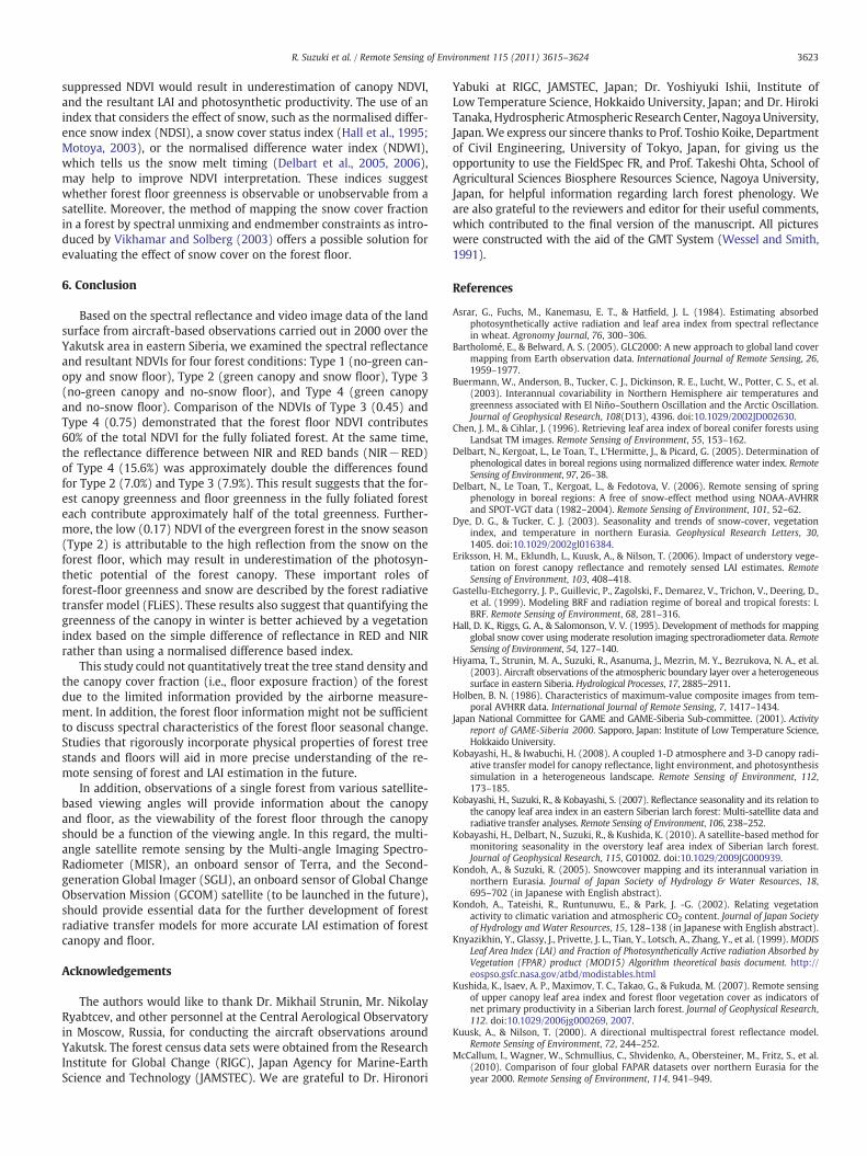
60°90° 120°

150°

60°(a)

60°(b)

0.0 0.1 0.2 0.3 0.4

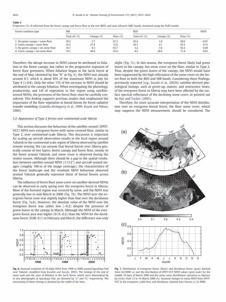
Table 5Proportion (%) of reflection from the forest canopy and forest floor in the red (RED) and near-infrared (NIR) bands, simulated using the FLiES model.

Forest-condition type NIR RED NDVI

Total ref. (%) Canopy (%) Floor (%) Total ref. (%) Canopy (%) Floor (%)

1: No-green canopy+snow floor 39.2 2.7 97.3 45.4 1.0 99.0 −0.072: Green canopy+snow floor 32.2 27.4 72.6 26.7 4.7 95.3 0.133: No-green canopy+no-snow floor 16.1 6.3 93.7 5.2 7.8 92.2 0.484: Green canopy+no-snow floor 19.1 44.4 55.6 4.2 28.6 71.4 0.63

3622 R. Suzuki et al. / Remote Sensing of Environment 115 (2011) 3615–3624

Therefore, the abrupt increase in NDVI cannot be attributed to folia-tion in the forest canopy, but rather to the progressive exposure offorest floor greenness. When foliation began in the larch forest atthe end of May (denoted by line “b” in Fig. 6), the NDVI was alreadyaround 0.7, which is about 85% of the maximum NDVI in July forType 4 (≥0.8). Only the other 15% of the increase in NDVI should beattributed to the canopy foliation. When investigating the phenology,productivity, and LAI of vegetation in this region using satellite-sensed NDVIs, the greenness of the forest floor must be carefully con-sidered. This finding supports previous studies that emphasised theimportance of the floor vegetation in boreal forests for forest radiativetransfer modelling (Gastellu-Etchegorry et al., 1999; Kuusk and Nilson,2000).

5.2. Appearance of Type 2 forests over continental-scale Siberia

This section discusses the behaviour of the satellite-sensed (SPOT-VGT) NDVI over evergreen forest with snow-covered floor, similar toType 2, over continental-scale Siberia. This discussion is importantfor scaling up aircraft observation results in the local region aroundYakutsk to the continental scale region of Siberia observed by satelliteremote sensing. We can assume that boreal forests over Siberia gen-erally consist of two layers, forest canopy and forest floor, similar tothe forest around Yakutsk, and snow cover is observed during thewinter season. Although there should be a gap in the spatial resolu-tion between satellite-sensed NDVI (1/112°) and aircraft-sensed im-ages (roughly 100 m of the image coverage), the characteristics ofthe forest landscape and the resultant NDVI behaviour observedaround Yakutsk generally represent those of boreal forests acrossSiberia.

The influence of forest floor snow cover on satellite-derived NDVIscan be observed in early spring over the evergreen forest in Siberia.Most of the forested region was covered by snow, and the NDVI wasgenerally low in mid-March in 2000 (Fig. 7b). The NDVI over the ev-ergreen forest zone was slightly higher than that over the deciduousforest (Fig. 7a,b). However, the absolute value of the NDVI over theevergreen forest was rather low (~0.2) despite the presence ofgreen leaves in the canopy in March. Although the NDVI of the ever-green forest area was higher (0.15–0.2) than the NDVI for the decid-uous forest (0.08–0.1) in February and March, the difference was only

0.0

0.2

0.4

0.6

0.8

1.0

ND

VI

a b a b a b

1998 1999 2000J F M A M J J A S O N D J F M A M J J A S O N D J F M A M J J A S O N D

Fig. 6. Seasonal evolution of 10-daily NDVI from 1998 to 2000 around Spasskaya Padnear Yakutsk (modified from Kondoh and Suzuki, 2005). The timings of the end ofsnow melt and the start of foliation in the larch forest, which were determined byin situ photographs at Spasskaya Pad, are denoted by “a” and “b,” respectively. Theuncertainty of these timings is denoted by the width of the lines.

slight (Fig. 7c). In this season, the evergreen forest likely had greenleaves in the canopy, but snow cover on the floor, similar to Type 2.Thus, despite the green leaves of the canopy, the NDVI would havebeen suppressed by the high reflectance of the snow cover on the for-est floor in both the RED and NIR bands. Considering these findings,previously reported (e.g., Suzuki et al., 2003b) satellite-derived phe-nological timings, such as green-up, mature, and senescence times,of the evergreen forest in Siberia may have been affected by the sur-face spectral reflectance of the declining snow cover, as pointed outby Dye and Tucker (2003).

Therefore, for more accurate interpretation of the NDVI distribu-tion over an evergreen boreal forest, the floor snow cover, whichmay suppress the NDVI measurement, should be considered. The

0.0

0.2

0.4

0.6

0.8

ND

VI

J F M A M J J A S O N Dmonth

(c)

Fig. 7. Distribution of evergreen forest (black) and deciduous forest (grey) derivedfrom GLC2000 (a) and the distribution of SPOT-VGT NDVI values (grey scale) for themiddle 10 days of March 2000 and the snow cover distribution (presence or absenceby circle) from 13 to 19 March 2000 (b). Seasonal changes in mean NDVI from SPOT-VGT in the evergreen (solid line) and deciduous (dashed line) forests (c) in 2000.

3623R. Suzuki et al. / Remote Sensing of Environment 115 (2011) 3615–3624

suppressed NDVI would result in underestimation of canopy NDVI,and the resultant LAI and photosynthetic productivity. The use of anindex that considers the effect of snow, such as the normalised differ-ence snow index (NDSI), a snow cover status index (Hall et al., 1995;Motoya, 2003), or the normalised difference water index (NDWI),which tells us the snow melt timing (Delbart et al., 2005, 2006),may help to improve NDVI interpretation. These indices suggestwhether forest floor greenness is observable or unobservable from asatellite. Moreover, the method of mapping the snow cover fractionin a forest by spectral unmixing and endmember constraints as intro-duced by Vikhamar and Solberg (2003) offers a possible solution forevaluating the effect of snow cover on the forest floor.

6. Conclusion

Based on the spectral reflectance and video image data of the landsurface from aircraft-based observations carried out in 2000 over theYakutsk area in eastern Siberia, we examined the spectral reflectanceand resultant NDVIs for four forest conditions: Type 1 (no-green can-opy and snow floor), Type 2 (green canopy and snow floor), Type 3(no-green canopy and no-snow floor), and Type 4 (green canopyand no-snow floor). Comparison of the NDVIs of Type 3 (0.45) andType 4 (0.75) demonstrated that the forest floor NDVI contributes60% of the total NDVI for the fully foliated forest. At the same time,the reflectance difference between NIR and RED bands (NIR−RED)of Type 4 (15.6%) was approximately double the differences foundfor Type 2 (7.0%) and Type 3 (7.9%). This result suggests that the for-est canopy greenness and floor greenness in the fully foliated foresteach contribute approximately half of the total greenness. Further-more, the low (0.17) NDVI of the evergreen forest in the snow season(Type 2) is attributable to the high reflection from the snow on theforest floor, which may result in underestimation of the photosyn-thetic potential of the forest canopy. These important roles offorest-floor greenness and snow are described by the forest radiativetransfer model (FLiES). These results also suggest that quantifying thegreenness of the canopy in winter is better achieved by a vegetationindex based on the simple difference of reflectance in RED and NIRrather than using a normalised difference based index.

This study could not quantitatively treat the tree stand density andthe canopy cover fraction (i.e., floor exposure fraction) of the forestdue to the limited information provided by the airborne measure-ment. In addition, the forest floor information might not be sufficientto discuss spectral characteristics of the forest floor seasonal change.Studies that rigorously incorporate physical properties of forest treestands and floors will aid in more precise understanding of the re-mote sensing of forest and LAI estimation in the future.

In addition, observations of a single forest from various satellite-based viewing angles will provide information about the canopyand floor, as the viewability of the forest floor through the canopyshould be a function of the viewing angle. In this regard, the multi-angle satellite remote sensing by the Multi-angle Imaging Spectro-Radiometer (MISR), an onboard sensor of Terra, and the Second-generation Global Imager (SGLI), an onboard sensor of Global ChangeObservation Mission (GCOM) satellite (to be launched in the future),should provide essential data for the further development of forestradiative transfer models for more accurate LAI estimation of forestcanopy and floor.

Acknowledgements

The authors would like to thank Dr. Mikhail Strunin, Mr. NikolayRyabtcev, and other personnel at the Central Aerological Observatoryin Moscow, Russia, for conducting the aircraft observations aroundYakutsk. The forest census data sets were obtained from the ResearchInstitute for Global Change (RIGC), Japan Agency for Marine-EarthScience and Technology (JAMSTEC). We are grateful to Dr. Hironori

Yabuki at RIGC, JAMSTEC, Japan; Dr. Yoshiyuki Ishii, Institute ofLow Temperature Science, Hokkaido University, Japan; and Dr. HirokiTanaka, Hydrospheric Atmospheric Research Center, NagoyaUniversity,Japan.We express our sincere thanks to Prof. Toshio Koike, Departmentof Civil Engineering, University of Tokyo, Japan, for giving us theopportunity to use the FieldSpec FR, and Prof. Takeshi Ohta, School ofAgricultural Sciences Biosphere Resources Science, Nagoya University,Japan, for helpful information regarding larch forest phenology. Weare also grateful to the reviewers and editor for their useful comments,which contributed to the final version of the manuscript. All pictureswere constructed with the aid of the GMT System (Wessel and Smith,1991).

References

Asrar, G., Fuchs, M., Kanemasu, E. T., & Hatfield, J. L. (1984). Estimating absorbedphotosynthetically active radiation and leaf area index from spectral reflectancein wheat. Agronomy Journal, 76, 300–306.

Bartholomé, E., & Belward, A. S. (2005). GLC2000: A new approach to global land covermapping from Earth observation data. International Journal of Remote Sensing, 26,1959–1977.

Buermann, W., Anderson, B., Tucker, C. J., Dickinson, R. E., Lucht, W., Potter, C. S., et al.(2003). Interannual covariability in Northern Hemisphere air temperatures andgreenness associated with El Niño–Southern Oscillation and the Arctic Oscillation.Journal of Geophysical Research, 108(D13), 4396. doi:10.1029/2002JD002630.

Chen, J. M., & Cihlar, J. (1996). Retrieving leaf area index of boreal conifer forests usingLandsat TM images. Remote Sensing of Environment, 55, 153–162.

Delbart, N., Kergoat, L., Le Toan, T., L'Hermitte, J., & Picard, G. (2005). Determination ofphenological dates in boreal regions using normalized difference water index. RemoteSensing of Environment, 97, 26–38.

Delbart, N., Le Toan, T., Kergoat, L., & Fedotova, V. (2006). Remote sensing of springphenology in boreal regions: A free of snow-effect method using NOAA-AVHRRand SPOT-VGT data (1982–2004). Remote Sensing of Environment, 101, 52–62.

Dye, D. G., & Tucker, C. J. (2003). Seasonality and trends of snow-cover, vegetationindex, and temperature in northern Eurasia. Geophysical Research Letters, 30,1405. doi:10.1029/2002gl016384.

Eriksson, H. M., Eklundh, L., Kuusk, A., & Nilson, T. (2006). Impact of understory vege-tation on forest canopy reflectance and remotely sensed LAI estimates. RemoteSensing of Environment, 103, 408–418.

Gastellu-Etchegorry, J. P., Guillevic, P., Zagolski, F., Demarez, V., Trichon, V., Deering, D.,et al. (1999). Modeling BRF and radiation regime of boreal and tropical forests: I.BRF. Remote Sensing of Environment, 68, 281–316.

Hall, D. K., Riggs, G. A., & Salomonson, V. V. (1995). Development of methods for mappingglobal snow cover using moderate resolution imaging spectroradiometer data. RemoteSensing of Environment, 54, 127–140.

Hiyama, T., Strunin, M. A., Suzuki, R., Asanuma, J., Mezrin, M. Y., Bezrukova, N. A., et al.(2003). Aircraft observations of the atmospheric boundary layer over a heterogeneoussurface in eastern Siberia. Hydrological Processes, 17, 2885–2911.

Holben, B. N. (1986). Characteristics of maximum-value composite images from tem-poral AVHRR data. International Journal of Remote Sensing, 7, 1417–1434.

Japan National Committee for GAME and GAME-Siberia Sub-committee. (2001). Activityreport of GAME-Siberia 2000. Sapporo, Japan: Institute of Low Temperature Science,Hokkaido University.

Kobayashi, H., & Iwabuchi, H. (2008). A coupled 1-D atmosphere and 3-D canopy radi-ative transfer model for canopy reflectance, light environment, and photosynthesissimulation in a heterogeneous landscape. Remote Sensing of Environment, 112,173–185.

Kobayashi, H., Suzuki, R., & Kobayashi, S. (2007). Reflectance seasonality and its relation tothe canopy leaf area index in an eastern Siberian larch forest: Multi-satellite data andradiative transfer analyses. Remote Sensing of Environment, 106, 238–252.

Kobayashi, H., Delbart, N., Suzuki, R., & Kushida, K. (2010). A satellite-based method formonitoring seasonality in the overstory leaf area index of Siberian larch forest.Journal of Geophysical Research, 115, G01002. doi:10.1029/2009JG000939.

Kondoh, A., & Suzuki, R. (2005). Snowcover mapping and its interannual variation innorthern Eurasia. Journal of Japan Society of Hydrology & Water Resources, 18,695–702 (in Japanese with English abstract).

Kondoh, A., Tateishi, R., Runtunuwu, E., & Park, J. -G. (2002). Relating vegetationactivity to climatic variation and atmospheric CO2 content. Journal of Japan Societyof Hydrology and Water Resources, 15, 128–138 (in Japanese with English abstract).

Knyazikhin, Y., Glassy, J., Privette, J. L., Tian, Y., Lotsch, A., Zhang, Y., et al. (1999).MODISLeaf Area Index (LAI) and Fraction of Photosynthetically Active radiation Absorbed byVegetation (FPAR) product (MOD15) Algorithm theoretical basis document. http://eospso.gsfc.nasa.gov/atbd/modistables.html

Kushida, K., Isaev, A. P., Maximov, T. C., Takao, G., & Fukuda, M. (2007). Remote sensingof upper canopy leaf area index and forest floor vegetation cover as indicators ofnet primary productivity in a Siberian larch forest. Journal of Geophysical Research,112. doi:10.1029/2006jg000269, 2007.

Kuusk, A., & Nilson, T. (2000). A directional multispectral forest reflectance model.Remote Sensing of Environment, 72, 244–252.

McCallum, I., Wagner, W., Schmullius, C., Shvidenko, A., Obersteiner, M., Fritz, S., et al.(2010). Comparison of four global FAPAR datasets over northern Eurasia for theyear 2000. Remote Sensing of Environment, 114, 941–949.

3624 R. Suzuki et al. / Remote Sensing of Environment 115 (2011) 3615–3624

Motoya, K. (2003). Spectral characteristic-based vegetation and snow indices onvarious surfaces in the airborne multi-spectral scanner (AMSS) two-altitudeobservation in 2001. Journal of Japan Society of Hydrology & Water Resources, 16,408–419 (in Japanese with English abstract).

Myneni, R. B., Hoffman, S., Knyazikhin, Y., Privette, J. L., Glassy, J., Tian, Y., et al. (2002).Global products of vegetation leaf area and fraction absorbed PAR from year one ofMODIS data. Remote Sensing of Environment, 83, 214–231.

Myneni, R. B., Nemani, R. R., & Running, S. W. (1997). Estimation of global leaf areaindex and absorbed PAR using radiative transfer model. IEEE Transactions onGeoscience and Remote Sensing, 35, 1380–1393.

Nemani, R. R., Keeling, C. D., Hashimoto, H., Jolly, W. M., Piper, S. C., Tucker, C. J., et al.(2003). Climate-driven increases in global terrestrial net primary productionfrom 1982 to 1999. Science, 300, 1560–1563.

Nilson, T., & Peterson, U. (1991). A forest canopy reflectance model and a test case.Remote Sensing of Environment, 37, 131–142.

Ohta, T., Hiyama, T., Tanaka, H., Kuwada, T., Maximov, T. C., Ohata, T., et al. (2001).Seasonal variation in the energy and water exchanges above and below a larchforest in eastern Siberia. Hydrological Processes, 15, 1459–1476.

O'Neill, N. T., Zagolski, F., Bergeron, M., Royer, A., Miller, J. R., & Freemantle, J. (1997).Atmospheric correction validation of CASI images acquired over the BOREASsouthern study area. Canadian Journal of Remote Sensing, 23, 143–162.

Peddle, D. R., Hall, F. G., & LeDrew, E. F. (1999). Spectral mixture analysis andgeometric-optical reflectance modelling of boreal forest biophysical structure.Remote Sensing of Environment, 67, 288–297.

Peddle, D. R., Brunke, S. P., & Hall, F. G. (2001). A comparison of spectral mixtureanalysis and ten vegetation indices for estimating boreal forest biophysicalinformation from airborne data. Canadian Journal of Remote Sensing, 27, 627–635.

Piao, S., Wang, X., Ciais, P., Zhuz, B., Wang, T., & Liu, J. (2011). Changes in satellite-derived vegetation growth trend in temperate and boreal Eurasia from 1982 to2006. Global Change Biology. doi:10.1111/j.1365-2486.2011.02419.x.

Pinty, B., Gobron, N., Widlowski, J. -L., Gerstl, S., Verstraete, M., Antunes, M., et al.(2001). Radiation transfer model intercomparison (RAMI) exercise. Journal ofGeophysical Research, 106(D11), 11937–11956.

Pisek, J., & Chen, J. M. (2009). Mapping forest background reflectivity over NorthAmerica with Multi-angle Imaging SpectroRadiometer (MISR) data. Remote Sensingof Environment, 113, 2412–2423.

Rautiainen, M. (2005). Retrieval of leaf area index for a coniferous forest by inverting aforest reflectance model. Remote Sensing of Environment, 99, 295–303.

Sellers, P. J., Los, S. O., Tucker, C. J., Justice, C. O., Dazlich, D. A., Collaz, G. J., et al. (1996).A revised land surface parameterization (SiB2) for atmospheric GCMs. Part II. Thegeneration of global fields of terrestrial biophysical parameters from satellitedata. Journal of Climate, 9, 706–737.

Shulze, E. -D., Shulze, W., Kelliher, F. M., Vygodskaya, N. N., Ziegler, W., Kobak, K. I., et al.(1995). Aboveground biomass and nitrogen nutrition in a chronosequence ofpristine Dahurian Larix stands in eastern Siberia. Canadian Journal of ForestResearch, 25, 943–960.

Strahler, A. (Ed.). (1999). MODIS Land Cover Product Algorithm Theoretical BasisDocument (ATBD) Version 5.0.

Suzuki, R., Sugimoto, A., Numaguti, A., Ichiyanagi, K., Kurita, N., Takata, K., et al.(2001a). Plant area index observation at surface sites around Yakutsk duringIOP2000. Proceedings of GAME-Siberia Workshop, GAME-Siberia Sub-committee(pp. 79–80). Japan National Committee for GAME.

Suzuki, R., Yoshikawa, K., & Maximov, T. C. (2001b). Phenological photographs ofSiberian larch forest from 1997 to 2000 at Spasskaya Pad, Republic of Sakha, Russia.http://www.jamstec.go.jp/iorgc/hcorp/data/database/products/phenol/index.htm

Suzuki, R., Hiyama, T., Asanuma, J., Koike, T., & Ohata, T. (2003a). Airborne Spectral Re-flectance Data of the Land Surface around Yakutsk in IOP2000 in Dataset for Waterand Energy Cycle in Siberia (version 1). Yokohama, Japan: GAME-Siberia and Fron-tier Observational Research System for Global Change.

Suzuki, R., Nomaki, T., & Yasunari, T. (2003b). West–east contrast of phenology andclimate in northern Asia revealed using a remotely sensed vegetation index. Inter-national Journal of Biometeorology, 47, 126–138.

Suzuki, R., Hiyama, T., Asanuma, J., & Ohata, T. (2004). Land surface identification nearYakutsk in eastern Siberia using video images taken from a hedgehopping aircraft.International Journal of Remote Sensing, 25, 4015–4028.

Suzuki, R., Xu, J., &Motoya, K. (2006). Global analyses of satellite-derived vegetation indexrelated to climatological wetness andwarmth. International Journal of Climatology, 26,425–438.

Suzuki, R., Masuda, K., & Dye, D. G. (2007). Interannual covariability between actualevapotranspiratoin and PAL and GIMMS NDVIs of northern Asia. Remote Sensingof Environment, 106, 387–398.

Tarpley, J. D., Schneider, S. R., & Money, R. L. (1984). Global vegetation indices from theNOAA-7 meteorological satellite. Journal of Climate and Applied Meteorology, 23,491–494.

Tucker, C. J. (1979). Red and photographic infrared linear combinations for monitoringvegetation. Remote Sensing of Environment, 8, 127–150.

Tucker, C. J., Slayback, D. A., Pinzon, J. E., Los, S. O., Myneni, R. B., & Taylor, M. G.(2001). Higher northern latitude normalized difference vegetation index andgrowing season trends from 1982 to 1999. International Journal of Biometeorology,45, 184–190.

Vicente-Serrano, S. M., Grippa, M., Delbart, D., Le Toan, T., & Kergoat, L. (2006).Influence of seasonal pressure patterns on temporal variability of vegetationactivity in central Siberia. International Journal of Climatology, 26, 303–321.

Vikhamar, D., & Solberg, R. (2003). Snow-cover mapping in forests by constrainedlinear spectral unmixing of MODIS data. Remote Sensing of Environment, 88,309–323.

Wessel, P., & Smith, W. H. F. (1991). Free software helps map and display data. EOSTransactions, American Geophysical Union, 72(441), 445–446.

Widlowski, J. -L., Robustelli, M., Disney, M., Gastellu-Etchegorry, J. -P., Lavergne, T.,Lewis, P., et al. (2008). The RAMI On-line Model Checker (ROMC): A web-basedbenchmarking facility for canopy reflectance models. Remote Sensing of Environ-ment, 112, 1144–1150.