Dear Yale Readers, This paper is not really a work of economic history. Rather, it is an exercise in exploring correlations between past things and present outcomes, with some work on intermediate periods to examine WHY we see such a correlation. That being said, there are interesting historical questions that reside at the heart of this exercise that we are currently grappling with, that deserve more attention in the paper, and that would benefit greatly from any inputs you can provide. I am far less concerned (or convinced, myself) about the “outcomes today” part of the paper, although that is obviously where the hook is and where so much of this “historical persistence” literature lies. So even if you detest that sort of economic history – and I know many attending surely do – bear with me as I focus on what I think are the historically interesting parts of the project and the things that we are currently doing in those areas. The draft I am circulating is very much a work in progress that will soon be massively revised. So any and all comments are very much appreciated. Regards, Steve Nafziger Williamstown, MA March 2016

Long-Run Consequences of Labor Coercion:Evidence from Russian Serfdom ⇤

Johannes C. Buggle† Steven Nafziger‡

This paper examines the long-run consequences of Russian serfdom. Weuse novel data measuring the intensity of labor coercion at the district level in1861. Our results show that a greater legacy of serfdom is associated with lowereconomic well-being today. We apply an IV strategy that exploits the transfer ofserfs from monastic lands in 1764 to establish causality. Exploring mechanisms,we find a positive correlation between the earlier experience of serfdom and pre-Soviet urbanization and land inequality, with negative implications for humancapital investment and agglomeration over the long-run.(Keywords: Labor Coercion, Serfdom, Development, Russia, Persistence. JEL-Codes: N33, N54, O10, O43)

Throughout human history, “coercive” labor relations have been widespreadphenomena, from Roman slavery to forced cotton harvests in contemporaryUzbekistan.1 Economists have long argued that unfree labor generates eco-nomic inefficiencies, but whether impediments persist once the institution isabolished has only recently entered the discussion. In this paper, we study

⇤We are grateful to Yann Algan, Quamrul Ashraf, Roger Bartlett, Elena Nikolova, SergeiGuriev, Katia Zhuravskaya, and seminar participants at Sciences Po and the WEast Workshopon Economic History and Development in Budapest for helpful comments. We also thank theEBRD for providing the geo-coded LiTS survey waves for 2006 and 2010. Parts of this researchwere undertaken while Buggle was visiting the Economics Department at UC Berkeley, whosehospitality is appreciated. Please see the Online Appendix for additional material and results.All errors remain our own.

†Department of Economics, Sciences Po, 27 Rue des Saints-Peres, 75007 Paris, France.johannes.buggle@sciencespo.fr

‡Department of Economics, Williams College, Schapiro Hall, 24 Hopkins Hall Dr.,Williamstown, MA 01267. snafzige@williams.edu

1Around 21 million people in the world today are in forced labor, coerced either by privateindividuals or the state according to the International Labor Organization ILO 2012 GlobalEstimate of Forced Labour.

2

whether institutions of unfree labor can have economic consequences long af-ter their demise, using one of the most prominent examples of coerced laborin recent history: Russian serfdom. We uncover a robust negative relationshipbetween this institutional heritage and economic development today and go onto investigate the mechanisms underlying this persistence. Our results provideadditional evidence on the economic importance of institutional legacies andadd to the emerging empirical literature documenting adverse long-run conse-quences of forced labor (e.g. Engerman and Sokoloff (1997), Dell (2010), Nunn(2008b), Acemoglu, García-Jimeno and Robinson (2012), Acharya, Blackwelland Sen (2013)).2

Russian serfdom was a system of labor coercion that existed from the 16thcentury to 1861, and has been perceived as a crucial institution in the region’seconomic history (Acemoglu and Robinson, 2012).3 Indeed, at a time when theIndustrial Revolution was fundamentally changing the economies of WesternEurope, around 50% of peasants in European Russia were obliged to work forthe landowning nobility or pay them a portion of their income in the form ofquit-rent. Amid broader efforts at modernization following the Crimean War,the Russian state initiated the legal emancipation of serfs in 1861, followedby a drawn out process of land reform that transferred property rights (gener-ally assigned to the communal village) and associated payment obligations tothe newly freed peasants. The changes that these formerly privately “owned”peasants went through may be contrasted with the experience of the rest of thepeasantry, who resided on state or Imperial family-owned lands prior to 1861,and who saw a reform process in the 1860s that changed relatively little of theirlandholdings or obligations. These peasants possessed more land and faced amore liberal (at least on average) policy and institutional environment prior tothe 1860s, and their reform experience solidified these differences in the shortand medium term. In this paper, we leverage this heterogeneity within the pre-

2Differences exist between Russian serfdom and forced labor in other contexts. First ofall, serfs tended to enjoy considerable autonomy in how they allocated their time unlike, forexample, the majority of American slaves. Second, although there were important exceptions,Russian serfs differed little from their masters with respect to race, ethnicity, or religion. Serfswere a distinct social category that was fundamentally based on ownership and control of labor.This means that race or ethnicity as mechanisms of persistence, certainly important in the Northand South American cases, can largely be excluded in the Russian one.

3Slavery had a long history in Kievan and Muscovite Russia. The laws and customs re-garding debt servitude and other forms of personal obligation helped structure those that laterformalized serfdom (Hellie (1982)).

3

1861 peasantry to identify longer-run consequences of serfdom.Newly collected district (uezd) level data from a tax census conducted in

the late 1850’s allow us to map the variation in the share of the population whowere serfs across the European part of Imperial Russia. To test for differences inlong-run economic outcomes across districts with high and low levels of histor-ical serfdom, we match our measure of serfdom’s intensity with outcome datafrom today (especially from the Life in Transition Survey (LiTS)) and from in-termediate periods. We document that households in districts where serfdomwas widespread before 1861 are poorer today, conditional on a large set of localbio-geographic characteristics, household variables, proxies for early develop-ment, and provincial fixed effects. According to our OLS estimates, a standarddeviation increase in the share of the population who were serfs is associatedwith 10 - 14% lower average household consumption today.

OLS estimates would be biased, however, if unobserved district character-istics influenced where serrfdom was more common and, at the same time, af-fected economic outcomes in the long-run. To address these omitted variableconcerns, we make use of plausibly exogenous variation in the extent of serfdomderived from the transfer of church land and serfs to state control by Catherinethe Great in the 18th century. Church serfs, which had been subject to largelythe same constraints as privately owned serfs, were, as a result of this reform,integrated into the “state peasantry” by the early 19th century. We exploit thishistorical experiment by using the geographic distribution of monasteries (themost significant holder of church property) before the onset of Catherine’s re-forms in 1764 to instrument for the intensity of serfdom at the district leveljust prior to emancipation. The instrument is a strong predictor of serfdom’sintensity, and the IV results again show that the prevalence of the historical in-stitution is negatively related to current household expenditures, with estimatedcoefficients larger than in the OLS specifications.4

Critically, we then move on to investigate the robustness of our basic resultsand explore the potential channels behind this correlation. We show that agricul-tural suitability of the land only matters for long-run well-being in areas whereserfdom did not spread and confirm the negative relationship between serfdom’sintensity and long-run outcomes by studying household asset ownership and byemploying night-time luminosity in 2008 at the (historical) district level as a

4We discuss several possible reasons for the larger IV coefficients.

4

proxy for the level of development. Using data from 1700 to 1989, we showthat cities in areas with relatively more serfs had lower populations and did notcatch up over time. In addition, we find a negative relationship between serfdomand the number of factories and industrial output per worker just after emanci-pation. These findings imply possible agglomeration and local spillover effectsthat perpetuated themselves over time, thus constituting one potential link be-tween serfdom and modern outcomes. In terms of other possible channels ofpersistence, we first show that serfdom was positively correlated with land in-equality and the share of land owned by the nobility in 1905. Given the possibleassociation between land inequality (and the presence of a landed elite) andthe provision of local rural public goods, this very likely slowed developmentprior to the initiation of collectivization and other Soviet-era policies. Indeed,consistent with a literature that links unequal landownership to reduced humancapital investment (possibly with inter-generational implications) in other con-texts, serfdom is associated with fewer schools per district in 1856, lower schoolenrollment in 1880 and 1894, and lower educational attainment today. In termsof modern public goods, we do not find differences in access to basic servicessuch water, electricity and heating, which are all fairly widely distributed. How-ever, former serf areas had a significantly lower road and rail density in the lateSoviet period, which is consistent with an agglomeration interpretation. Finally,we find little evidence for a distinctive set of cultural attitudes in areas whereserfdom was more prevalent, which is consistent with the absence of differentracial, ethnic, or religious identities in former serf regions.

Whether serfdom generated a legacy for subsequent Russian economic de-velopment has long been a topic of scholarly interest. Alexander Gerschenkron(1966), among others, attributed the slow pace of development in late-TsaristRussia to serfdom and particular features of the emancipation process that seem-ingly perpetuated many institutional restrictions in the countryside (also seeDennison (2011) and Lenin (1911)). However, empirical work on Russian serf-dom and emancipation, both in general and in terms of documenting subse-quent effects, is relatively limited. One notable exception is Markevich andZhuravskaya (2015), who estimate that provinces with above average levels ofserfdom (as a share of the total population) were growing relatively faster afteremancipation. In a related work, Nafziger (2013) shows that the emancipationprocess largely defined the subsequent structure of factor endowments and land

5

prices in the countryside prior to the Revolution of 1917. However, these studiesdo not consider the possible omitted variable bias that our IV strategy addresses.

At the same time, whether economic differences between high and low serfregions persisted beyond the Imperial period has not previously been studied.This is not surprising given that the Soviet Union stands between then andnow, and that regime completely revolutionized Russian economic, political,and social institutions. However, researchers have found long-run effects ofinstitutional variation in other contexts, even in the face of subsequent and dra-matic changes (e.g. Nunn (2008a) and Michalopoulos and Papaioannou (2013)).Given the evident importance of serfdom for Russia’s economic development,both prior to 1861 and before 1917, it is particularly valuable to investigate theextent to which this institutional regime generated long-run effects. If one es-tablishes a correlation between past serfdom and present outcomes, identifyingthe underlying mechanisms of persistence is obviously imperative, particularlyas such an exercise may suggest historical factors underlying the economic dif-ficulties that countries in this region have faced since the end of communist rule.In this way, our study also contributes to the literature on historical developmentand persistence (Nunn (2013) provides an excellent survey). While we empha-size the agglomeration implications of a local legacy of serfdom, our empiricalinvestigation also provides novel evidence on how factor inequality, especiallyin land, can stifle long-run economic development through initial constraints oninvestment in human capital and public goods (as in Galor, Moav and Vollrath(2009), Galor and Moav (2006), and others).

Section 1 describes the historical background, including the measurementand determinants of the geographic variation in serfdom. Section 2 estimatesthe impact of serfdom on long-run development. Section 3 investigates potentialchannels of persistence. Section 4 concludes.

1 The History, Measurement, and Determinants of Serfdom

1.1 Historical Background 5

Russian serfdom emerged as a set of formal institutional constraints and in-formal practices in the 16th and 17th centuries. In return for service to the Tsars

5This account is drawn from various studies. A good summary is provided in Moon (1999).

6

before and during this period of state expansion, the elite received large landgrants that came with the right to draw upon the labor of the resident popula-tion. However, with competition among the servitors and the ease of fleeingto open land, it was difficult for the land-owning class to exploit their laboringpeasantry. The high land-labor ratio motivated the land-owning nobility to act toreduce the mobility of the peasantry and to increase control over various aspectsof their lives. These attempts came to be supported by the state through vari-ous decrees, culminating in the 1649 Ulozhenie that sharply constrained peasantmobility and formalized the legal rights of the serf-owning nobility. Over the18th century, further measures affirmed the control of the nobility over theirpeasants, with the 1762 “emancipation” of the nobility freeing the serf-owningclass from any corresponding obligations for state service. By 1800, the legaland institutional context of Russian serfdom was firmly in place.

Serfdom varied widely across estates but can be described by certain com-mon characteristics. First of all, serfs constituted a distinct social estate apartfrom the nobility, the clergy, and even other peasants, and they faced substantiverestrictions on their personal, family, and community autonomy (Wirtschafter(1997)). This had implications for their rights under Russian civil, criminal,and property law, including restrictions on land ownership. Serf owners heldsubstantial authority over the daily lives of their peasants, allowing them tointervene in marriage, employment, educational, religious, judicial, and othermatters.6 Second, serf-owners demanded seigniorial rents and obligations. Ex-traction took the form of labor obligations, cash or in-kind payments, or a com-bination of the two. On many estates, owners actively managed the labor deci-sions of their serfs on and off the estate, either in person or through managerialstaff. Such estates generally possessed demesnes, with labor on the owner’s landcompensated by the granting of use-rights to the rest of the property. On otherestates, serfs granted substantial freedom to allocate their labor as they saw fit.This latter variant was more common in less agriculturally productive regions,where owners tended to transfer the use of all estate land to the serfs in returnfor cash or in-kind payments.

Despite substantial, estate by estate, variation, these attributes suggest aninstitutional regime that was antithetical to economic development. The labor,

6From the early 19th century, the nobility’s autonomy included the possibility of emanci-pating their serfs on their own terms. This option was exercised relatively infrequently.

7

property, and education decisions of serfs were often circumscribed, resulting indisincentives for investment, the misallocation of labor and other resources, im-pediments to the adoption of better agricultural techniques, and a host of otherconstraints. And given the prevalence of serfdom, these microeconomic condi-tions may have slowed Russian industrial development and kept rural incomeslow. Many contemporary observers acknowledged the disincentives for eco-nomic growth that the institution generated prior to 1861. Indeed, supportersof the status quo argued for continuing the institution less in economic termsthan in order to maintain the Imperial regime, to defend Slavic traditions, and tosupport some form of elite tutelage over masses ill-equipped for freedom.7

Despite a long scholarly debate, there is remarkably little causal evidenceon the economic impact of serfdom (and emancipation). Dennison (2011) hasrecently argued that serfdom generated adverse distributional and growth ef-fects, although her conclusions are based on evidence from a single large estate.Soviet works (e.g. Koval’chenko (1967)) marshaled considerable data to arguethat the serf economy was in decline prior to 1861. However, the materials thatthese scholars employed tended to be rather selective, and their Marxist orien-tation placed the argument before the evidence. Domar and Machina (1984)utilized more comprehensive information on the price of land with and withoutresident peasants to argue that serfdom was profitable to the nobility and, there-fore, worth defending when emancipation was proposed. But profitability is notthe same as efficiency, and there is little hard evidence on the correspondinggrowth implications of serfdom from a neoclassical perspective. An importantexception is the recent work of Markevich and Zhuravskaya (2015), who evalu-ate the impact of serfdom by looking at differential economic changes betweenareas with more or fewer serfs before and after 1861. They argue for stronglynegative effects of serfdom, although this conclusion is based on relatively lim-ited provincial data, and they do not explicitly address the possibility of omittedvariables.8 Thus, despite limited causal evidence, most scholarship on Russianserfdom asserts that it undermined economic development while it existed.

Considerably more empirical attention has been paid to the short and

7See the discussions and citations in Emmons (1968), Field (1976), and Khristoforov(2011).

8In general, Markevich and Zhuravskaya (2015), and related works such as Nafziger(2012b), face a key difficulty in evaluating the immediate economic impact of Russian serf-dom: the dearth of quality data prior to 1861.

8

medium-term consequences of emancipation in the half century before the Bol-shevik Revolution. Soviet studies (e.g. Litvak (1972)) argued that emancipationand the accompanying land reforms actually worsened former serf land holdingsand imposed considerable new burdens on the rural economy.9 This literatureargued that while former serfs retained land as part of the reforms, they receivedthese property rights collectively through the newly formalized commune, theland they received was often different (worse) in amount and quality from whatthey had before, and they were held jointly responsible for (possibly higher thanbefore) mortgage-like payments in return. In contrast, more recent studies suchas Hoch (2004) and Kashchenko (2002) argue that the majority of former serfswere made better off – at least in terms of factor endowments and obligations –than Soviet studies asserted.10

In his influential interpretation, Gerschenkron (1966) went beyond pre/post1861 factor endowment comparisons to emphasize the negative implications ofthe peasantry’s joint liability and communal property rights for agricultural pro-ductivity and labor mobility after 1861. While centered on the experience of theformer serfs, Gerschenkron and others writing in this vein (i.e. Allen (2003))have tended to focus on broader institutional impediments that characterized allpeasants. Although emancipation and subsequent land measures were perhapsmost dramatic for the former serfs, by the 1880s, the different types of peas-ants were administratively unified and possessed similar institutions of commu-nal self-governance, (generally) collective property rights, and joint liability fortaxes and land payments. Of course, such nominal similarities may have hid-den many persistent de facto differences in the conditions faced by the differentpeasant groups. Indeed, as Nafziger (2013) shows using more detailed data thanprevious studies, landholdings were smaller, land inequality was greater, and theassociated land and tax obligations were higher in districts with relatively moreformer serfs, well into the 20th century.

Gerschenkron (1966) argued that the famous Stolypin land reforms of theearly 20th century (named for the Prime Minister Pëtr Stolypin) fostered betterincentives in peasant agriculture by offering mechanisms for consolidating plotsand exiting the commune. But these were just the first steps in a series of dra-

9None of these Soviet works were based on causal identification.10All of these studies have relied on empirical evidence that was not necessarily represen-

tative, was too aggregate to identify differences, or covered an intermediate stage of a verycomplicated and drawn-out reform process.

9

matic changes that would deeply impact rural Russian society over the rest ofthe century: the Bolshevik Revolution, collectivization, famine, World War II,and the slow collapse of the agricultural sector from the 1970s onward. Noneof these changes explicitly or differentially targeted former serfs, but they mayhave generated or reinforced important and persistent effects that built upon pre-existing geographic, institutional, and economic differences among peasants.

1.2 Measuring 19th–Century Serfdom

While serfdom was a defining feature of Russian society by the early 19thcentury, not all peasants resided on noble–owned land or were subject to quasi-feudal exploitation by the gentry. By the 1850s, a minority of peasants weredirectly subject to the nobility. Peasants residing on state or Romanov family-owned land (we refer to the latter as “court peasants”) were governed by spe-cific administrative bodies, possessed more land and freedom to engage in con-tracts, and were generally only liable for direct (and lower) tax-like obligations(Nafziger (2013)). As we noted above, some of these factor endowment differ-ences persisted in the decades after 1861, and different groups of peasants mayhave faced persistently different institutional conditions, despite the nominaladministrative and legal convergence following serf emancipation.

The geography of serfdom is well known, but scholars have generally fo-cused on specific estates or small geographic areas or relied on coarse statisticsfrom aggregate data. With regards to the latter, Hoch and Augustine (1979)and Kabuzan (2002) document serfdom by relying on data generated by ten taxcensuses undertaken between 1719 and 1858.11 These two studies report totalsindicating that the share of serfs in the Imperial population crested at just over50% at the turn of the 18th century, before falling to roughly 35% just beforeemancipation.

We study serfdom at the administrative level of the district (uezd), the largestsub-unit of a province.12 Relying on the 10th tax census of 1858, as reported inTroinitskii (1982 (1861), we construct our main indicator of serfdom’s intensity,Serfs, perc. of pop, which divides the total number of serfs by the total district

11Initiated by Peter the Great, these collected data on the populations that were obligated fortaxes of different types.

12To do this, we digitized a 19th century district-level map of European Russia.

10

population.13 Since we do not know the total number of peasants per district,we use the overall population as a denominator.14 The resulting indicator covers495 historical districts (in 50 provinces) in European Russia without Poland andFinland.

While over 90% of districts contained some serfs just before emancipation,in only few did the share of serfs in the total population exceed 80%.15 Inour study area, serfs averaged 38% of a district’s population.16 Figure 1 showsthe underlying variation across European Russia.17 The map indicates that theinstitution was largely concentrated in a band from Kiev to the upper Volga.However, even in high-serfdom areas, and even within provinces, there wasconsiderable variation in the share of the population subjugated to the nobility.

1.3 Determinants of Serfdom

A number of potential explanatory factors comes to mind in consideringthe determinants of the “incidence” of serfdom.18 First, the location of a dis-trict likely determined whether the spread of serfdom reached a locality or not.As Muscovy expanded away from Moscow before 1700, state service was of-ten rewarded with the allocation of land in newly incorporated areas, but thispracticed eased over the 18th century. Therefore, we consider the direct (log)distance from each district centroid to Moscow We also take into account a dis-trict’s geographic location by controlling for the latitude and longitude of itscentroid.

Variation in land productivity might have led to differences in the demandfor coerced labor or in the desirability of land in return for state service. An im-

13Unfortunately, district-level population totals from the 10th tax census are unavailable. Asa result, we draw on Bushen (1863), which provides the total populations for 1863. Given thepossibility of emancipation-induced migration, this might seem to introduce some measurementerror. However, the 1863 population figures were based on administrative records of the tax-paying population, which were unlikely to have been quickly adjusted (and which may havelargely relied upon the 10th tax census).

14An ideal intensity measure would use the number of peasants as denominator. Anothersource of potential measurement error might arise from using a snapshot of serfdom in 1858,which neglects prior changes in serfdom’s intensity.

15See the distribution function in Figure A1 in the Appendix.16See Table A1 in the Appendix for all relevant summary statistics.17The picture is very similar if the denominator only includes the rural population.18All of the variables mentioned in this section are summarized in the Appendix Table A1,

where further details can be found.

11

Figure 1: Spatial Distribution of Serfs as Share of Population c. 1858.

portant proxy for agricultural productivity is the suitability of the soil for grow-ing crops. As grains, and in particular wheat, were dominant in the Empire’sagriculturally productive areas, we use modern geo-spatial data to produce atime-invariant measure of the land’s suitability for growing wheat (we also con-sider soil suitability for growing other grains such as oat, barley and rye). Otherenvironmental conditions might have affected local agricultural productivity, themobility of the population (hence, the incentives for maintaining serfdom), andlocal incomes. Therefore, we also construct variables that measure the fractionof land covered with forest today, the ruggedness of the terrain, and the presenceof a river. 19

A prominent hypothesis regarding the emergence of serfdom states that ahigh land-labor ratio made feudal labor coercion more likely (Domar (1970)).20

Scarcity provided the incentives to tie labor to the land by creating and perpet-

19These environmental variables are obtained from the FAO-GAEZ database. Soviet author-ities did engage in agricultural and resource practices that may have impacted these and otherenvironmental conditions over the 20th century. Such changes were relatively small, likely un-related to the incidence of serfdom, and mostly occurred outside of European Russia.

20More recently, Acemoglu and Wolitzky (2011) studies coercive labor relations in aprincipal-agent framework, arguing that labor scarcity affects both demand for, and the outsideoptions of, workers and, thus, has an ambiguous effect on coercion.

12

uating institutional constraints on mobility. Although the employment of serfson private estates was not exactly a choice variable (since the laws governingpeasant labor mobility applied to all estates), and the spread of noble landhold-ing was likely driven by geography and Muscovite expansion, this frameworkmight have some relevance if estate owners were more willing to free their peas-ants prior to 1861 in areas where labor was relatively more abundant. To accountfor this possibility, we generally control for population density in 1600, takenfrom the History Database of the Global Environment (HYDE), version 3.1.21

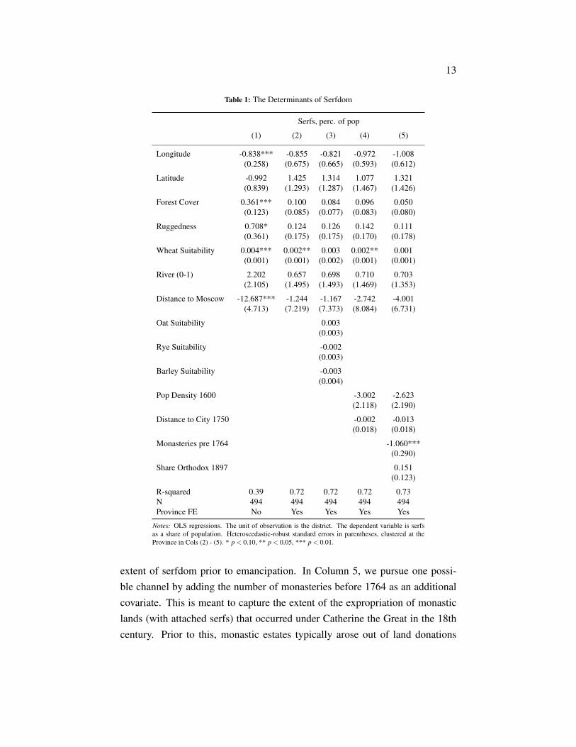
In Table 1, we explore the possible determinants of the distribution of serf-dom through OLS regressions that rely on either across-district (Column 1) orwithin-province variation (Column 2). The coefficients on longitude and dis-tance to Moscow are negative, consistent with the direction of Muscovite ex-pansion mattering. The suitability for growing wheat is generally the strongestpredictor of serfdom’s intensity and displays a positive association. This is con-sistent with the spread of noble estates to relatively agriculturally productive ar-eas, although when we add other crops in Column (3), wheat suitability loses itssignificance. Although districts with higher population density in 1600 display,on average, smaller population shares of serfs (Column 4), this difference is sta-tistically insignificant, suggesting that mechanisms other than Domar’s were atwork. Indeed, we find that districts that were further away from a city in 1750 (asreported in the dataset of Bairoch, Batou and Chèvre (1988)), a proxy for earlydevelopment and economic activity, show a lower incidence of serfdom (Col-umn 4). Again, this would suggest a process by which noble estates were setup in more advantageous areas. We also find that a district’s province explainsa large part of serfdom’s intensity. Moving from the cross-district specifica-tion in Column 1 to the provincial fixed-effect model of Column 2 increases theR-squared from 0.4 to 0.7 while significantly reducing the explanatory powerof longitude, the area covered with forest, and the distance to Moscow. Thus,provincial fixed effects largely control for geography and the direction of Mus-covite expansion. Wheat suitability retains significance, and almost all of thecoefficients have the same signs as in Column 1.

As evident in even the fixed-effect model, other factors surely influenced the

21This database provides a raster for estimated population densities for different points intime with a spatial resolution of 5-minutes. It has been previously used in economics by Fenske(2013).

13

Table 1: The Determinants of Serfdom

Serfs, perc. of pop

(1) (2) (3) (4) (5)

Longitude -0.838*** -0.855 -0.821 -0.972 -1.008(0.258) (0.675) (0.665) (0.593) (0.612)

Latitude -0.992 1.425 1.314 1.077 1.321(0.839) (1.293) (1.287) (1.467) (1.426)

Forest Cover 0.361*** 0.100 0.084 0.096 0.050(0.123) (0.085) (0.077) (0.083) (0.080)

Ruggedness 0.708* 0.124 0.126 0.142 0.111(0.361) (0.175) (0.175) (0.170) (0.178)

Wheat Suitability 0.004*** 0.002** 0.003 0.002** 0.001(0.001) (0.001) (0.002) (0.001) (0.001)

River (0-1) 2.202 0.657 0.698 0.710 0.703(2.105) (1.495) (1.493) (1.469) (1.353)

Distance to Moscow -12.687*** -1.244 -1.167 -2.742 -4.001(4.713) (7.219) (7.373) (8.084) (6.731)

Oat Suitability 0.003(0.003)

Rye Suitability -0.002(0.003)

Barley Suitability -0.003(0.004)

Pop Density 1600 -3.002 -2.623(2.118) (2.190)

Distance to City 1750 -0.002 -0.013(0.018) (0.018)

Monasteries pre 1764 -1.060***(0.290)

Share Orthodox 1897 0.151(0.123)

R-squared 0.39 0.72 0.72 0.72 0.73N 494 494 494 494 494Province FE No Yes Yes Yes Yes

Notes: OLS regressions. The unit of observation is the district. The dependent variable is serfsas a share of population. Heteroscedastic-robust standard errors in parentheses, clustered at theProvince in Cols (2) - (5). * p < 0.10, ** p < 0.05, *** p < 0.01.

extent of serfdom prior to emancipation. In Column 5, we pursue one possi-ble channel by adding the number of monasteries before 1764 as an additionalcovariate. This is meant to capture the extent of the expropriation of monasticlands (with attached serfs) that occurred under Catherine the Great in the 18thcentury. Prior to this, monastic estates typically arose out of land donations

14

from wealthy donors and the state, suggesting that their distribution paralleledthe allocation of private holdings. Following this expropriation, these peasantswere eventually transferred into the state peasantry, thus generating a policy-driven source of variation in the share of serfs in the total population c. 1860.The coefficient that we estimate on this variable turns out to be negative andhighly statistically significant. This effect remains when we control for the localOrthodox population share, measured by later census data in 1897. We return tothis important finding below when we exploit the presence of monasteries priorto 1764 as a plausibly exogenous source of variation in serfdom measured priorto 1861.

2 Serfdom and Long-Run Development

2.1 Defining Outcomes

Constructing outcomes for our long-run investigation is challenging. In-come per capita is not available at a unit of analysis comparable to our historicaldata on serfdom. Moreover, our historical sample encompasses several currentEastern European countries, in addition to the Russian Federation.

Household Expenditure and Wealth To circumvent these data limitations,we construct our main outcome variables from the 2006 and 2010 waves ofthe Life in Transition Survey (LiTS).22 We use the geo-locations of the PrimarySampling Units (PSU) of the two waves to precisely locate respondents fromseveral modern countries within the historical districts of Imperial Russia.23

Our main indicator for modern economic development is household expendi-ture per capita, which is only assessed in the 2006 wave. Household headsreported spending over a 30-day recall period for food and consumption goods,such as clothing, transport, and recreation, and over a 12-month recall periodfor investments and durable goods such as education, healthcare, and furniture.Expenditures are adjusted for the size of the household to create a measure of

22The LiTS is collected by the European Bank of Reconstruction to assess household andindividual well-being in transition countries.

23Figure A3 of the Appendix shows the PSU locations overlaying the variation in histor-ical serfdom. Summary statistics of our outcome variables are displayed in Table A1 of theAppendix, which also contains additional information on how are we construct them.

15

economic well-being per capita.24 As household expenditure is strictly positiveand skewed, we use its logarithm. 25

An advantage of LiTS is the availability of data on other individual andhousehold characteristics that potentially affect our outcomes of interest. Inour specifications, we control for household composition in terms of householdsize, the share of household members younger than 18, the share of householdmembers older than 60, and the share of male household members. We also uti-lize the religion of the respondent, an indicator variable for whether the primarysampling unit is defined as rural or urban, a dummy for the LiTS survey wave,and other respondent characteristics.26

2.2 Estimation Strategy

To assess the effect of serfdom on modern socio-economic outcomes, webegin with the following OLS regression:

yi,d,p = a +b ⇤ ser f domi,d,p +X ‘i,d,p ⇤w + province_ f ep + ei,d,p (1)

where i represents the unit of analysis, d refers to the historical district, and pindicates the historical province. ser f domi,d,p denotes our variable of concern,the share of serfs out of the total population in a (historical) district d, locatedin province p, and linked to modern unit of observation i. The coefficient ofinterest is b , which gives the reduced form relationship between the incidenceof serfdom and modern outcomes.

The matrix Xi,d,p includes household-level and survey controls (householdsize, share aged 0-18, share aged 60+, share male, religion, and indicators forrural/urban and LiTS wave, where relevant), location of the PSU, and variables

24The expenditures are expressed in US Dollars. Although, this variable relies on a recallmethod, the accuracy is remarkably good when compared to directly measured household con-sumption data (Zaidi et al. (2009)).

25In addition to our main outcome, we draw on LiTS to construct a measure of durableasset ownership and access to basic local public goods in the settlement of residence. We findsimilar results using this outcome (Table A2 of the Appendix). An alternative measure of localeconomic well-being is night-time luminosity, as measured by satellite pictures of the earthover a series of nights. Our findings are robust to using night-time luminosity and are reportedin Table A4 of the Appendix.

26In LiTS, the section on the household’s economic situation is answered by the householdhead, while other questions on attitudes, education, religion and labor are answered by a ran-domly selected household member. Whenever we use individual level responses provided bythis randomly selected member, we additionally control for their age, age sq. and gender.

16

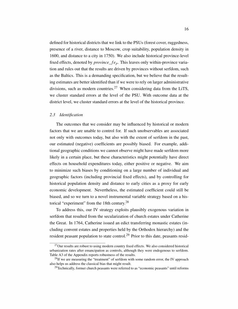
defined for historical districts that we link to the PSUs (forest cover, ruggedness,presence of a river, distance to Moscow, crop suitability, population density in1600, and distance to a city in 1750). We also include historical province-levelfixed effects, denoted by province_ f ep. This leaves only within-province varia-tion and rules out that the results are driven by provinces without serfdom, suchas the Baltics. This is a demanding specification, but we believe that the result-ing estimates are better identified than if we were to rely on larger administrativedivisions, such as modern countries.27 When considering data from the LiTS,we cluster standard errors at the level of the PSU. With outcome data at thedistrict level, we cluster standard errors at the level of the historical province.

2.3 Identification

The outcomes that we consider may be influenced by historical or modernfactors that we are unable to control for. If such unobservables are associatednot only with outcomes today, but also with the extent of serfdom in the past,our estimated (negative) coefficients are possibly biased. For example, addi-tional geographic conditions we cannot observe might have made serfdom morelikely in a certain place, but these characteristics might potentially have directeffects on household expenditures today, either positive or negative. We aimto minimize such biases by conditioning on a large number of individual andgeographic factors (including provincial fixed effects), and by controlling forhistorical population density and distance to early cities as a proxy for earlyeconomic development. Nevertheless, the estimated coefficient could still bebiased, and so we turn to a novel instrumental variable strategy based on a his-torical “experiment” from the 18th century.28

To address this, our IV strategy exploits plausibly exogenous variation inserfdom that resulted from the secularization of church estates under Catherinethe Great. In 1764, Catherine issued an edict transferring monastic estates (in-cluding convent estates and properties held by the Orthodox hierarchy) and theresident peasant population to state control.29 Prior to this date, peasants resid-

27Our results are robust to using modern country fixed effects. We also considered historicalurbanization rates after emancipation as controls, although they were endogenous to serfdom.Table A3 of the Appendix reports robustness of the results.

28If we are measuring the “treatment” of serfdom with some random error, the IV approachalso helps us address the classical bias that might result.

29Technically, former church peasants were referred to as “economic peasants” until reforms

17

ing on church and monastic land were subject to many of the same constraintsas privately owned serfs. Indeed, one professed reason for the reform was thatthe state was concerned about the especially exploitative conditions faced bythe church peasants (Zakharova (1982)).30 The 1764 decree secularized churchand monastic lands in Siberia and the central provinces of Russia, with latermeasures in the 18th and early 19th centuries doing likewise for Western andSouthwestern provinces.31 Following these reforms, the majority of monasticinstitutions were closed or consolidated, with those remaining receiving a rela-tively low level of support directly from the state.

Catherine’s 1764 reform transferred approximately 2 million church peas-ants (over 10% of the peasant population at that time) to state oversight andeventual membership in the state peasantry.32 If the original establishment ofchurch properties roughly paralleled the granting of populated land for state ser-vice (or was correlated with the unobservable determinants of the latter), thenthe geographic distribution of the expropriated estates may be interpreted as anexogenous source of variation in the presence of state peasants by the 1850s.33

The historical literature on Russian monasticism supports this interpretation:while some pre-1400 monastic settlements were initially established as remotehermitages, the greater number of monasteries, convents, and other church es-tates that emerged from the 15th to 18th centuries largely obtained their propertythrough grants from the Tsar and other large landowners as Muscovy grew into

of the 1830s integrated them with the rest of the state peasantry. On occasion below, we refer tothese varied church properties as monastic estates or land as a shorthand.

30We know of no direct evidence that monasteries played any special role in promotinglocal human capital accumulation among church peasants prior to 1764. Following the reforms,monastic institutions possibly did possess wealth available to support local economic activity,but it unlikely that this was significantly more than other large property holders.

31As noted by Zinchenko (1985), the Western provinces exhibited extensive property hold-ings among Orthodox and non-Orthodox religious institutions into the 19th century, with secu-larization occurring only in response to ethnic-religious unrest (particularly the Polish Rebellionof 1830–31) and as part of the broader state peasant reforms in the 1840s (de Madariaga (1981)and Zakharova (1982)). Our results hold if we focus only on the provinces affected by the 1764law.

32See Zakharova (1982), who refers to the changes wrought by the original act. These peas-ants were largely spread over the often dispersed properties of approximately 500 monasteries.

33Kamenskii (1997) writes of the peasants on expropriated church estates peasants that,“They were relieved of their labor obligations to the religious institutions, saw and increasein the size of their landed allotments and now found it easier to engage in trade and hand-craft.”. The subsequent improvement in the lives of the former church peasants is discussed byZakharova (1982).

18

an Empire.34 Although there are surely unobserved and location-specific factorsthat lay behind the granting of certain properties to church institutions, concernsabout the exclusion restriction should be mitigated by considering the extent ofexpropriated land aggregated over a district.

Our measure of this expropriation is the total number of monasteries per dis-trict that stopped functioning in or before 1764, compiled from Zverinskii (2005(1897).35 For the instrument to be valid, it needs to be strongly correlated withserfdom’s intensity. As we already showed in Column 3 of Table 1, the share ofserfs was indeed significantly lower in districts where the number of monasteriesprior to 1764 was high. In our results tables, we also report the Kleibergen-PaapWald F statistic of the first stage, which is always above 10 and ranges from 12to 169. Table 2 investigates the first-stage relationship in more detail. Column 1shows the coefficient of the baseline first stage relationship (-1.060). Columns2 and 3 re-estimate the first-stage but adjusts the instrument by population inColumn 2 and area in Column 3. In either regression the instrument is a neg-ative and significant predictor of serfdom – to ease interpretation, we focus onthe number of monasteries below (while controlling for other characteristics ofthe districts). Column 4 tests for robustness of the first-stage relationship ex-cluding provinces that were not subject to the 1764 decree. Columns 5 and 6show that districts with below median distance to Moscow display a larger re-duction in serfdom (-1.061) than districts that are further away (-0.732), poten-tially reflecting a stronger enforcement of the decree around the capital. Finally,the first-stage coefficient is larger for districts with above-median suitability forgrowing wheat (-1.228 vs -0.825) – see Columns 7 and 8.

A valid instrument should affect the outcomes of inter-est only through its effect on serf intensity, or, more formally,corr(Monasteriespre1764d,p,c,ei,d,p,c = 0) conditional on the set of ob-servable controls and province fixed effects. Although this is not strictlytestable, we do find that the geographic distribution of these monasteries was

34For example, see Kloss (2013), Ostrowski (1986), and Weickhardt (2012). Romaniello(2000) remarks on the geographically parallel processes of monastic and state “colonization,”especially in the Volga Region. In more settled areas, a significant amount of monastic land wasinitially collateral posted by gentry borrowers who defaulted on their loans from monasteries.

35See Figure A2 in the Appendix for a spatial representation of the number of monasteriesper district. Of course, we would prefer to have the amount and location of all variants ofexpropriated church lands and the corresponding number of peasants, but such data are currentlyunavailable.

19

Tabl

e2:

Firs

tSta

gean

dC

ompl

iers

Serf

s,pe

rc.o

fpop

(1)

(2)

(3)

(4)

(5)

(6)

(7)

(8)

Defi

nitio

nsof

the

Inst

rum

ent

Reg

ions

affe

cted

byD

ecre

eD

ist.

Mos

cow

<MD

ist.

Mos

cow

>MW

heat

Suita

bilit

y<M

Whe

atSu

itabi

lity>

M

Mon

aste

ries

pre

1764

-1.0

60**

*-1

.046

***

-1.0

61**

*-0

.732

*-0

.825

***

-1.2

28**

*(0

.290

)(0

.341

)(0

.350

)(0

.421

)(0

.284

)(0

.354

)

Mon

aste

ries

pre

1764

p.tth

.-7

.156

**(3

.098

)

Mon

aste

ries

pre

1764

p.ar

ea-1

0135

.726

***

(356

7.39

5)

R-s

quar

ed0.

730.

710.

730.

720.

470.

810.

790.

73N

494

483

494

410

250

244

246

248

Not

es:

OLS

regr

essi

ons.

The

unit

ofob

serv

atio

nis

the

dist

rict.

The

depe

nden

tvar

iabl

eis

serf

sas

ash

are

ofpo

pula

tion.

All

regr

essi

ons

cont

rolf

orge

ogra

phic

cont

rols

that

are

latit

ude

and

long

itude

ofth

edi

stric

t,th

ear

eaof

the

dist

rictc

over

edby

fore

st,r

ugge

dnes

sof

the

dist

rict,

suita

bilit

yof

the

soil

forg

row

ing

whe

at,p

rese

nce

ofa

river

inth

edi

stric

t,an

ddi

stan

ceof

the

dist

rictc

entro

idto

Mos

cow

,pop

ulat

ion

dens

ityin

1600

,dis

tanc

eto

the

near

estc

ityin

1750

,sha

reof

Orth

odox

in18

97,a

sw

ella

sPr

ovin

cefix

edef

fect

s.H

eter

osce

dast

ic-r

obus

tsta

ndar

der

rors

inpa

rent

hese

s,cl

uste

red

atth

ePr

ovin

ce.*

p<

0.10

,**

p<

0.05

,***

p<

0.01

.

20

Table 3: Testing for Correlation of the Instrument with Early Development

Log City Population in

1600 1700 1750 1800 1850

(1) (2) (3) (4) (5)

Monasteries pre 1764 -0.001 0.003 0.026 0.030** 0.029*(0.033) (0.024) (0.017) (0.014) (0.015)

R-squared 0.25 0.31 0.27 0.12 0.10N 23 29 112 187 190

Notes: OLS regressions. The unit of observation is a city. The dependent variable is logcity population, taken from Bairoch, Batou and Chèvre (1988). All regressions controlfor geographic controls, which include latitude and longitude of the district, the area ofthe district covered by forest, ruggedness of the district, suitability of the soil for grow-ing wheat, presence of a river in the district, and (ln) distance of the district centroid toMoscow. Heteroscedastic-robust standard errors in parentheses, clustered at the district.* p < 0.10, ** p < 0.05, *** p < 0.01.

unrelated to other characteristics of serfdom, including the share of serfs onquit rent only (specifications not reported here). There is little evidence that themonastic institutions that remained after 1764 were especially wealthy, as statesupport was kept at a relatively low level.36 Along with the similarities in theexpansion of monastic and private holdings, this gives some assurance that ourexpropriation variable is not related to other unobservable factors that mightimpact long-run outcomes.37

In additional tests reported in Table 3, we examine whether the prevalenceof pre-1764 monasteries was correlated with other indicators of early economicdevelopment. In particular, we consider the population of cities in different cen-turies reported in Bairoch, Batou and Chèvre (1988) as an indicator of economicdevelopment. We do not find that monasteries were associated with larger citypopulations before 1764 (but only from 1800 onwards).38

36While the Church did play a role in providing basic schooling over the 19th century, thiswas typically done at the level of the village priest, rather than monastic bodies.

37Table A7 in the Appendix reports the estimated relationships between geographic controlsand our measure of monasteries. Monasteries were more prevalent closer to Moscow, in easternparts of provinces, and in areas less suitable for wheat. All of these factors likely reflect thetiming of settlement as Muscovite Russia expanded.

38The sample size varies as the dataset of Bairoch, Batou and Chèvre (1988) covers morecities. Unfortunately, few cities are reported prior to 1750, limiting the power of the regressionswith population data for the years before 1750 is limited.

21

2.4 Results

Household Expenditure The OLS estimates from equation (1) with the logof household expenditure as the dependent variable are reported in Panel A ofTable 4.

Table 4: Contemporary Household Expenditure

Log Equivalent Expenditure Per Capita

(1) (2) (3) (4) (5)

Panel A: OLS

Serf, perc. of pop (x100) -0.577*** -0.625*** -0.385** -0.506*** -0.267(0.162) (0.176) (0.182) (0.179) (0.188)

Panel B: Reduced Form

Monasteries pre 1764 0.029*** 0.033*** 0.018** 0.033*** 0.019**(0.007) (0.009) (0.009) (0.008) (0.008)

Panel C: IV

Serf, perc. of pop (x100) -1.901*** -1.728*** -1.328** -1.726*** -1.331**(0.388) (0.375) (0.555) (0.382) (0.539)

R-squared 0.41 0.42 0.44 0.42 0.44N 5605 5605 5605 5605 5605

F-stat 22.15 26.81 13.13 32.49 15.80

Base and Household Controls Yes Yes Yes Yes YesGeographic Controls No Yes Yes Yes Yes(ln) Pop Density 1600 No No Yes No YesDistance City 1750 No No Yes No YesShare Orthodox 1897 No No No Yes YesFE Province Province Province Province ProvinceCluster PSU PSU PSU PSU PSU

Notes: The unit of observation is the individual. The dependent variable is Log Equivalent Expenditure PerCapita, taken from LiTS wave 2006. All regressions control for a set of base controls (religious denominationof the respondent, LiTS survey wave and an indicator whether the PSU is rural or urban) and household controls(household size, share of household members aged 0-18, share of household members aged 60+, share of malehousehold members). Geographic controls are latitude and longitude of the PSU, area of the district covered byforest, ruggedness of the district, suitability of the soil for growing wheat, presence of a river in the district, and(ln) distance of the district centroid to Moscow. Heteroscedastic-robust standard errors in parentheses, clusteredat the primary sampling unit. * p < 0.10, ** p < 0.05, *** p < 0.01.

Overall, we find a large, negative, and statistically significant correlation be-tween serfdom’s intensity and this measure of economic well-being. In Column1, we control for household and survey controls, as well as province fixed ef-fects. The estimated coefficient becomes larger in absolute value but is equallysignificant in Column 2 when we control for the set of environmental conditionsthat are potentially correlated with the geographic spread of serfdom. In Column3 we add controls that proxy for early economic development, i.e. log popula-tion density in 1600 and the distance to the nearest city in 1750. The coefficient

22

only decreases in absolute terms. Finally, to help alleviate concerns about otherfactors possibly driving persistence, in particular religious differences related tothe presence of Orthodox monasteries (the primary target of Catherine’s mea-sures), the model of Column 4 includes the district-level share of the populationwho were mainstream (non Old Believer) Orthodox in 1897. This reduces thesize of estimated coefficient, but we can still reject the null at the 1 % signifi-cance level. Controlling for both past development and religion produces a non-significant coefficient of serfdom, however, as reported in Column 5. As PanelC shows, we estimate significant, negative coefficients throughout all IV speci-fications. Overall, these estimates are economically meaningful: a one standarddeviation increase in serfdom (around 25 percentage points) is associated witha lower level of average household expenditure, depending on the specification,of between about 10 and 15% in OLS and up to 38 % in the IV specificatons.39

There are several possible explanations for the different magnitudes of thecoefficients in the OLS and IV specifications. First, the larger estimates in the IVregressions may be a sign of omitted variables in the OLS specifications, whichare correlated with serfdom and long-run development in opposing directions,thus biasing the OLS coefficient downwards. If this is the case, our IV estimatesindicate the “true” causal relationship between serfdom and outcomes. Second,the smaller OLS coefficients may result from measurement error in the poten-tially endogenous variable (the population share of serfs) that the IV overcomes.Since we cannot know the precise mechanism of serfdom’s long-run impact, andour indicator is an admittedly crude measure of a heterogeneous institution, thisis a distinct possibility. Of course, the magnitude of the IV coefficients mayindicate that our instrument picks up other determinants of long-run economicdevelopment and, therefore, violates the exclusion restriction. This would betrue if the areas where the state or private landowners donated land to monas-teries were systematically different (i.e. better) than areas where only privateestates (and their serfs) existed, or if monasteries themselves influenced the pro-cess of long-run development. The evidence we present above and our readingof the historical literature suggests that both scenarios are unlikely.

A final possibility is that the IV estimates reflect a local average treatment

39Since the dependent variable is in logs, the estimated coefficients are presented as a per-centage change in the dependent variable given a one unit change in the independent variable(semi-elasticities).

23

effect for a subsample of districts that were affected by Catherine’s transfer and“complied” with it, while the OLS estimates averages over all areas. Rerunningthe OLS estimation with controls as in Column 3 for only those provinces thatchurch lands subject to the transfer increases the magnitude of the OLS coef-ficient from -0.39 to -0.92, while considering only districts with below mediandistance to Moscow similarly increases the OLS coefficient to -0.76. Thus, it isplausible that at least some of the increase in the magnitude of the coefficientcomes from the fact that the IV estimates represent a local average treatmentaffect for a subset of districts in which the monastic reform applied. Unfor-tunately, the exact explanation for the larger IV coefficients cannot be distin-guished empirically.40

The Differential Effect of Land Suitability in Serf and Non-Serf AreasThe OLS and IV regressions show a negative association between serfdom andhousehold-level economic outcomes today. Another strategy to estimate thelong-run effects of serfdom in a more indirect fashion is to differentiate the ef-fects of observable characteristics on long-run economic success in areas wherepeasants were more or less exploited under the institutional regime.41 We con-duct such exercise in the case of land suitability for agricultural production. Inthe absence of labor exploitation one would expect suitable land to be conduc-tive to economic development for many reasons, including forward linkages toindustrial production.

However, in areas where Russian serfdom remained prevalent until 1861,the positive effect of land quality on subsequent economic fortunes would likelybe impeded. Indeed, this is what Table 5 shows. Within provinces where serf-dom either never existed or ended much earlier (in particular the Baltics, whereemancipation occurred in 1819 under very different conditions),42 land suitabil-ity shows the expected positive and significant correlation with household ex-penditure in columns (1) and (2). If one in considers areas where serfdom waspresent, the previously positive impact of land turns negative and insignificant,see column (3) and (4).

40For a similar discussion of larger IV magnitudes compared to OLS estimations see Dell(2012) on the long-term effects of the Mexican Revolution.

41We thank Katia Zhuravskaya for this suggestion.42Here, non-serf provinces are Kurliand, Lifland, and Estliand.

24

Table 5: The Differential Effect of Land Suitability

(1) (2) (3) (4)Log Equivalent Expenditure Per Capita

No Serfdom Serfdom

Land Suitability 0.150*** 0.128** -0.023 -0.033for Growing Wheat (0.048) (0.049) (0.038) (0.033)

R-squared 0.28 0.29 0.43 0.44N 1708 1708 4095 4095(ln) Pop Density 1600 No Yes No YesDistance City 1750 No Yes No YesShare Orthodox 1897 No Yes No YesFE Province Province Province ProvinceCluster PSU PSU PSU PSU

Notes: The unit of observation is the individual. All regressions control for a set ofbase controls (religious denomination of the respondent, LiTS survey wave and anindicator whether the PSU is rural or urban) and household controls (household size,share of household members aged 0-18, share of household members aged 60+, shareof male household members), as well as geographic controls which are latitude andlongitude of the PSU, area of the district covered by forest, ruggedness of the district,presence of a river in the district, and (ln) distance of the district centroid to Moscow.Non-serf provinces are Kurliand, Lifland, and Estliand. Heteroscedastic-robust stan-dard errors in parentheses, clustered at the primary sampling unit. * p < 0.10, **p < 0.05, *** p < 0.01.

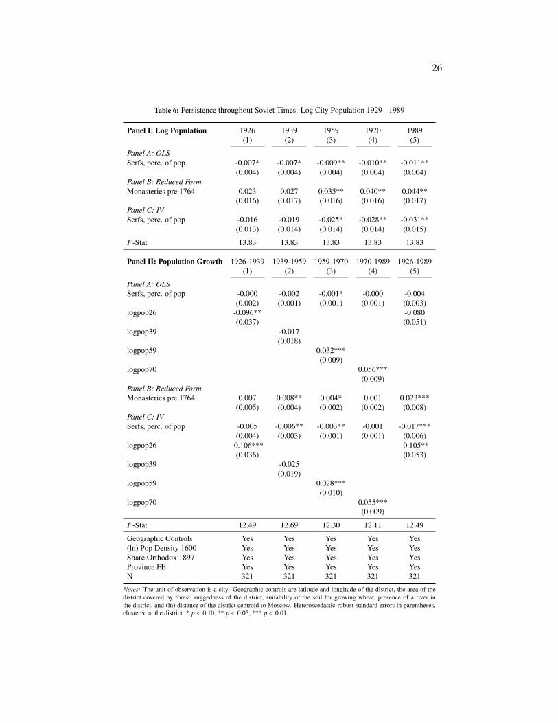
City Population in the Soviet Union When did the formerly serf areas fallbehind? And was there any process of convergence during the Soviet period?We investigate these questions using a sample of cities for which we can followtheir population over the 20th century.43 We rely on population data collected byAcemoglu, Hassan and Robinson (2011) for a sample of 321 cities documentedin the Soviet censuses of 1926, 1939, 1959, 1970 and 1989. After locating thesecities in our historical districts, we regress log population in each year on ourmeasure of serfdom. We find a negative association between city population andthe incidence of historical serfdom in the surrounding district for every year –see Panel I of Table 6. Increasing serfdom by one standard deviation reduces citypopulation by between 20% and 50% on average. Intriguingly, when compar-ing across years, the magnitude of the effect becomes larger later in the Sovietperiod. One speculative reason for this increasing gap is that areas with a highlevel of urbanization at the beginning of the period increasingly benefited fromsupportive Soviet policies over time. The well-known urban bias of the Com-munist leadership and centralized control over investment and factor allocation

43City population as a measure for economic development has been used extensively byeconomic historians in the absence of reliable economic data.

25

decisions certainly may have generated such pressures.The pattern of persistent differences in urbanization according to the expe-

rience of serfdom is also consistent with the results obtained from models usingcity growth as the dependent variable, controlling for the initial level of pop-ulation. We present results from such specifications in the bottom Panel II ofTable 6. Here, we again find that historical serfdom has a negative, althoughnot always significant, association with population growth. The implication isthat, if anything, former serf areas were falling further behind over the Sovietperiod. One can also see the long-run lack of catch-up city growth in Figure 2,in which we plot average log city population from 1750 to 1989 by quartiles ofserfdom.44 The gap in city population exists from 1750 on, narrows between1850 and 1929, but then widens until the end of the Soviet Union in 1989.

Figure 2: Avg City Population 1750-1989 and Serfdom (Quartiles)

3 Mechanisms

What mechanisms can explain the long-run effects of serfdom? In general,the literature has suggested a number of possibilities for why variation in histor-

44For this exercise, we combine data from Bairoch, Batou and Chèvre (1988) for 1750, 1800,1850 and Acemoglu, Hassan and Robinson (2011) for the later years. Note that the resultingpanel of cities is not balanced.

26

Table 6: Persistence throughout Soviet Times: Log City Population 1929 - 1989

Panel I: Log Population 1926 1939 1959 1970 1989(1) (2) (3) (4) (5)

Panel A: OLSSerfs, perc. of pop -0.007* -0.007* -0.009** -0.010** -0.011**

(0.004) (0.004) (0.004) (0.004) (0.004)Panel B: Reduced FormMonasteries pre 1764 0.023 0.027 0.035** 0.040** 0.044**

(0.016) (0.017) (0.016) (0.016) (0.017)Panel C: IVSerfs, perc. of pop -0.016 -0.019 -0.025* -0.028** -0.031**

(0.013) (0.014) (0.014) (0.014) (0.015)

F-Stat 13.83 13.83 13.83 13.83 13.83

Panel II: Population Growth 1926-1939 1939-1959 1959-1970 1970-1989 1926-1989(1) (2) (3) (4) (5)

Panel A: OLSSerfs, perc. of pop -0.000 -0.002 -0.001* -0.000 -0.004

(0.002) (0.001) (0.001) (0.001) (0.003)logpop26 -0.096** -0.080

(0.037) (0.051)logpop39 -0.017

(0.018)logpop59 0.032***

(0.009)logpop70 0.056***

(0.009)Panel B: Reduced FormMonasteries pre 1764 0.007 0.008** 0.004* 0.001 0.023***

(0.005) (0.004) (0.002) (0.002) (0.008)Panel C: IVSerfs, perc. of pop -0.005 -0.006** -0.003** -0.001 -0.017***

(0.004) (0.003) (0.001) (0.001) (0.006)logpop26 -0.106*** -0.105**

(0.036) (0.053)logpop39 -0.025

(0.019)logpop59 0.028***

(0.010)logpop70 0.055***

(0.009)

F-Stat 12.49 12.69 12.30 12.11 12.49

Geographic Controls Yes Yes Yes Yes Yes(ln) Pop Density 1600 Yes Yes Yes Yes YesShare Orthodox 1897 Yes Yes Yes Yes YesProvince FE Yes Yes Yes Yes YesN 321 321 321 321 321

Notes: The unit of observation is a city. Geographic controls are latitude and longitude of the district, the area of thedistrict covered by forest, ruggedness of the district, suitability of the soil for growing wheat, presence of a river inthe district, and (ln) distance of the district centroid to Moscow. Heteroscedastic-robust standard errors in parentheses,clustered at the district. * p < 0.10, ** p < 0.05, *** p < 0.01.

27

ical institutions – particularly coercive labor institutions – might generate long-run economic effects. These proposed mechanisms include asset and incomeinequality (e.g. Engerman and Sokoloff (1997), Nunn (2008a)), human capi-tal accumulation (e.g. Bertocchi and Dimico (2014)), and culture (e.g. Nunn(2012)).45 As in Acharya, Blackwell and Sen (2013), these channels may havepolitical implications (i.e. reinforcing the power of a local elite), with persis-tent consequences for local institutional development and economic policies.In this section, we explore which channels are relevant in the case of Russianserfdom.46

3.1 Inequality in the Distribution of Land

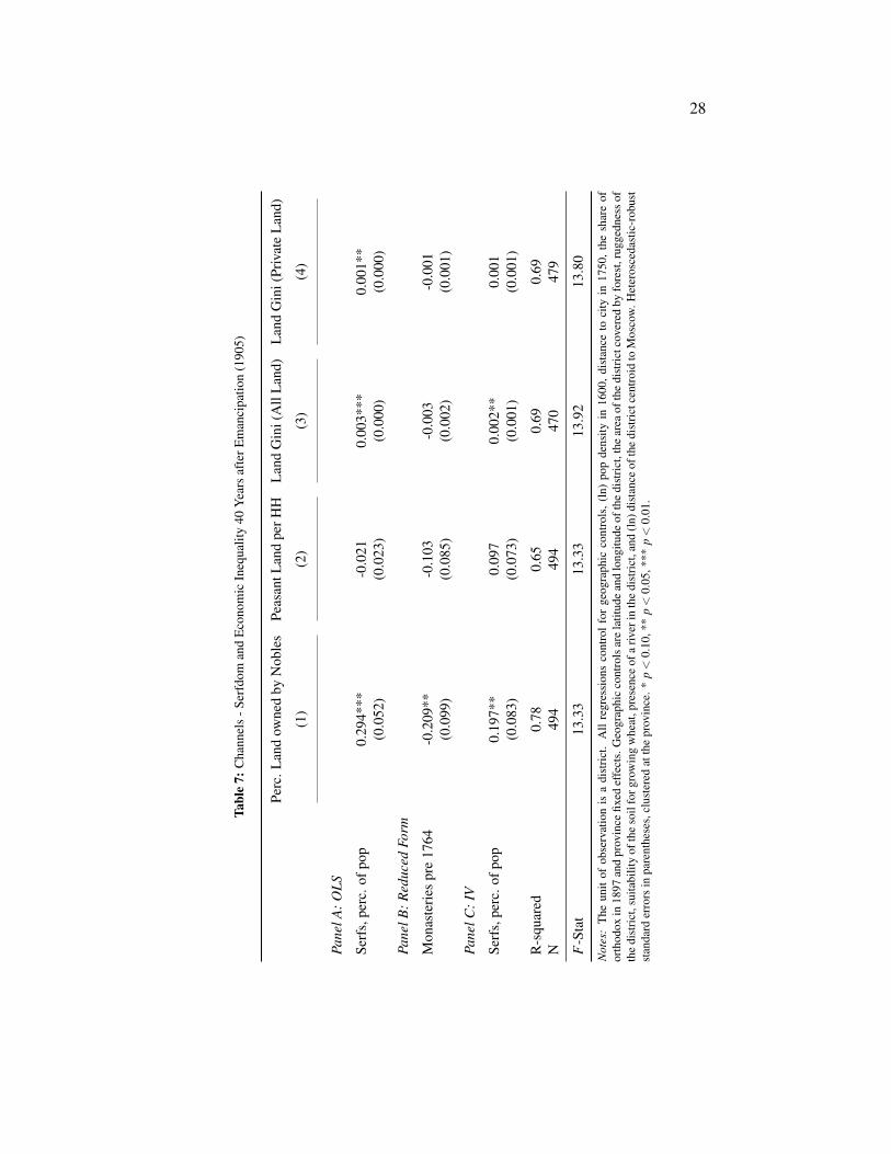
To begin, we investigate whether the incidence of serfdom was associatedwith subsequent inequality in the distribution of factors of production, particu-larly land. As the nobility owned the overwhelming majority of privately-heldland prior to emancipation, and subsequent reforms largely failed to undertakemuch redistribution, it would not be surprising to see persistently higher levelsof land inequality in regions with elevated levels of serfdom. Using measures ofinequality generated from district-level land statistics collected in 1905, we es-timate models similar to those in the previous sub-section. Our results stronglysupport a link between serfdom and land inequality through the end of the Im-perial period – see Table 7.47

We find that the incidence of serfdom is positively and significantly asso-ciated with the percentage of land owned by the nobles in 1905 (Column 1).48

45We find only limited evidence for differences in cultural attitudes today, consistent withthe absence of markers for former serf race or ethnicity. Regressions that investigate culturaldifferences are reported in the Appendix Table A6.

46Most of our “channel” variables are measured in the Imperial period, largely due to dataavailability and the change in administrative borders in the Soviet Union.

47These variables are described and summarized in greater detail in the Appendix and inNafziger (2013).

48Although not reported here, we also find that serfdom is negatively associated with theshare of all land held as communal allotments in 1905 (although with only marginal signifi-cance). This may capture a key element of the institutional climate fostered by the emancipationreforms: the reinforcement of the peasant land commune as a central pillar of rural society. Al-though the decision over whether to adopt communal property rights was mostly dictated by theemancipation statutes, the reforms did allow communities to adopt more individualized rights,and some took up this option in largely communal areas (Nafziger, 2013). By the 1880s, if notearlier, the formalization of the communal structure of rural Russian society applied in the sameway for peasants of different types.

28

Tabl

e7:

Cha

nnel

s-S

erfd

oman

dEc

onom

icIn

equa

lity

40Ye

ars

afte

rEm

anci

patio

n(1

905)

Perc

.Lan

dow

ned

byN

oble

sPe

asan

tLan

dpe

rHH

Land

Gin

i(A

llLa

nd)

Land

Gin

i(Pr

ivat

eLa

nd)

(1)

(2)

(3)

(4)

Pane

lA:O

LS

Serf

s,pe

rc.o

fpop

0.29

4***

-0.0

210.

003*

**0.

001*

*(0

.052

)(0

.023

)(0

.000

)(0

.000

)

Pane

lB:R

educ

edFo

rm

Mon

aste

ries

pre

1764

-0.2

09**

-0.1

03-0

.003

-0.0

01(0

.099

)(0

.085

)(0

.002

)(0

.001

)

Pane

lC:I

V

Serf

s,pe

rc.o

fpop

0.19

7**

0.09

70.

002*

*0.

001

(0.0

83)

(0.0

73)

(0.0

01)

(0.0

01)

R-s

quar

ed0.

780.

650.

690.

69N

494

494

470

479

F-S

tat

13.3

313

.33

13.9

213

.80

Not

es:

The

unit

ofob

serv

atio

nis

adi

stric

t.A

llre

gres

sion

sco

ntro

lfor

geog

raph

icco

ntro

ls,(

ln)

pop

dens

ityin

1600

,dis

tanc

eto

city

in17

50,t

hesh

are

ofor

thod

oxin

1897

and

prov

ince

fixed

effe

cts.

Geo

grap

hic

cont

rols

are

latit

ude

and

long

itude

ofth

edi

stric

t,th

ear

eaof

the

dist

rictc

over

edby

fore

st,r

ugge

dnes

sof

the

dist

rict,

suita

bilit

yof

the

soil

forg

row

ing

whe

at,p

rese

nce

ofa

river

inth

edi

stric

t,an

d(ln

)dis

tanc

eof

the

dist

rictc

entro

idto

Mos

cow

.Het

eros

ceda

stic

-rob

ust

stan

dard

erro

rsin

pare

nthe

ses,

clus

tere

dat

the

prov

ince

.*p<

0.10

,**

p<

0.05

,***

p<

0.01

.

29

More interesting is the result in Column 2, where we find no significant associ-ation between serfdom and the amount of land peasants received in the reformprocess of the 1860s per household in 1905 (Column 2; measured in desiatina,where 1=2.7 acres). This suggests that differences in the peasant emancipationprocesses did not lead to variation in property ownership, at least once geo-graphic factors are fully accounted for.

However, considering the distribution of land holdings, we find a positiverelationship between the incidence of serfdom and a Gini index covering hold-ings of all types of landed property (Column 3; private + communal land re-ceived through emancipation) and a Gini index covering private holdings ofnon-communal land only (Column 4), although the latter becomes insignificantin the IV specification. These estimated effects are large. A one standard devi-ation increase in serfdom corresponds to a greater share of land owned by thenobility (mean: 20.86; sd: 14.04) of between 5 (IV) and 7.5 (OLS) percentagepoints. Similarly, an increase in serfdom by one standard deviation is associatedwith an increase in the Gini index of all land holdings (mean: 0.49; sd: 0.16)by 0.05 (IV) to 0.075 (OLS). Thus, in areas with more serfdom, land holdingsremained relatively concentrated into the 20th century, particularly in the handsof the gentry class.

While the association between serfdom and subsequent land inequality iscompelling, how did this impede long-run economic growth, particularly afterthe Soviet policies largely dissolved preexisting property rights?49 Standard po-litical economy models (i.e. Galor, Moav and Vollrath (2009)) tend to suggestthat higher inequality created (political) impediments for policies related to hu-man capital accumulation and other public goods. This may occur via conflictover appropriate policies or through elite capture of local institutions, leading toa lower level of broad public good provision.50 Drawing on additional data, wecan evaluate whether our measures of human capital investment and and publicgoods are associated with the incidence of serfdom prior to 1861.

49A land inequality channel has been suggested for the case of slavery on plantationeconomies in the New World by Engerman and Sokoloff (1997), although Nunn (2008b) doesnot find empirical support for such a relationship in the U.S.

50See Nafziger (2011) for a discussion of public good provision in the Imperial Russian con-text that touches upon such inequality-related channels. Another prominent political economymechanism linking land inequality and development is (the absence of) political competition, assuggested by Besley, Persson and Sturm (2010) for the U.S. South. While possible, this seemsto be less directly relevant for the Russian case.

30

3.2 Schooling and Human Capital Investment

Table 8 Panel I examines the relationship between serfdom and educationaloutcomes before and after emancipation. To measure the historical expansionof human capital institutions, we examine the number of schools in a district in1856 (per thousand inhabitants), the percentage of rural boys and girls enrolledin primary schools in 1880, and total rural enrollment rates in 1894.51 As re-ported in Table 8, serf areas had fewer schools per thousand inhabitants beforeemancipation (in 1856), although the coefficient loses statistical significance inthe IV estimation (Column 1). We then find that serfdom was associated withlower enrollment rates of boys and girls in rural primary schools in 1880, andthe IV estimates show a statistically significant difference (Columns 2 and 3).52

A one standard deviation increase in serfdom reduces enrollment rate of boys byaround 30 %, and the enrollment rate of girls by around 35 %. We find similarresults when considering log rural enrollment rates of boys and girls measuredin 1894 (Column 4).

Similarly, Panel II of Table 8 considers modern educational outcomes takenfrom the LiTS. We examine whether the respondent completed secondary schooland whether they received some sort of post-secondary education (both dummyvariables). Our results show that the incidence of historical serfdom is signifi-cantly associated with a lower probability of completing secondary education,both in the OLS and IV regressions, with and without various controls (Columns1 and 2). Increasing our measure of serfdom by one standard deviation is as-sociated with a reduction in the likelihood that the respondent has completedsecondary education by 4.5 % (OLS) to 15 % (IV). Similarly, respondents inserf areas are also considerably less likely to have some education above thesecondary level (Columns 3 and 4).53 Taking the results of Panels I and II to-gether, we find evidence for a human capital mechanism behind the persistentdevelopment effects of serfdom. As we expand upon below, this may representa specific causal channel, or it could reflect the persistently lower level of struc-tural change (and consequent demand for education) in formerly serf areas.54

51See Nafziger (2012a) for more detail regarding these data.52We use the log of enrollment rates, as this variable is strictly positive but highly skewed.53We also investigated whether respondents profess a greater demand for education from the

government. As reported in the Appendix Table A5, individuals living in serf areas are lesslikely to mention education as the first government priority.

54A direct (or intergenerational) causal channel is perhaps unlikely given Soviet efforts to

31

Table 8: Channels - Education

Panel I Schools before 1856 (log) rural enrollment rateper 1000 pp boys in 1880 girls in 1880 boys and girls in 1894

(1) (2) (3) (4)

Panel A: OLS

Serfs, perc. of pop -0.001*** -0.001 -0.004 -0.001(0.000) (0.002) (0.003) (0.001)

Panel B: Reduced Form

Monasteries pre 1764 0.001 0.013* 0.016* 0.010**(0.001) (0.006) (0.009) (0.004)

Panel C: IV

Serfs, perc. of pop -0.001 -0.012** -0.014* -0.010**(0.001) (0.005) (0.009) (0.004)

R-squared 0.53 0.46 0.68 0.63N 489 492 492 494F-Stat 13.63 13.64 13.64 13.33

Geographic Controls Yes Yes Yes Yes(ln) Pop Density 1600 No Yes No YesDistance City 1750 No Yes No YesShare Orthodox 1897 No Yes No YesFE Province Province Province ProvinceCluster Province Province Province Province

Panel II At least secondary Above secondaryeducation in 2006 & 2010 education in 2006 & 2010

Panel A: OLS

Serf, perc. of pop (x100) -0.181*** -0.153** -0.158** -0.079(0.065) (0.070) (0.071) (0.075)

Panel B: Reduced Form

Monasteries pre 1764 0.010*** 0.009*** 0.009*** 0.005*(0.003) (0.004) (0.003) (0.003)

Panel C: IV

Serf, perc. of pop (x100) -0.607*** -0.661** -0.504*** -0.377*(0.204) (0.263) (0.164) (0.220)

R-squared 0.05 0.05 0.17 0.17N 12831 12831 12830 12830F-stat 115.24 59.16 115.24 59.16

Base and Household Controls Yes Yes Yes YesGeographic Controls Yes Yes Yes Yes(ln) Pop Density 1600 No Yes No YesDistance City 1750 No Yes No YesShare Orthodox 1897 No Yes No YesFE Province Province Province ProvinceCluster PSU PSU PSU PSU

Notes: Panel I: The unit of observation is a district. All regressions control for geographic controls, (ln) pop density in 1600, distanceto city in 1750, the share of Orthodox in 1897, and province fixed effects. Geographic controls are latitude and longitude of thedistrict, the area of the district covered by forest, ruggedness of the district, suitability of the soil for growing wheat, presence ofa river in the district, and (ln) distance of the district centroid to Moscow. Heteroscedastic-robust standard errors in parentheses,clustered at the province.Panel II: The unit of observation is the individual. All regressions control for a set of base controls (religious denomination of therespondent, LiTS survey wave and an indicator whether the PSU is rural or urban) and household controls (household size, share ofhousehold members aged 0-18, share of household members aged 60+, share of male household members). Geographic controls arelatitude and longitude of the district, the area of the district covered by forest, ruggedness of the district, suitability of the soil forgrowing wheat, presence of a river in the district, and (ln) distance of the district centroid to Moscow. Heteroscedastic-robust standarderrors in parentheses, clustered at the principal sampling unit. * p < 0.10, ** p < 0.05, *** p < 0.01.

32

3.3 Public Goods and Infrastructure Density

We also investigate the density of the road and railway networks during theSoviet period (Columns 1-4 of Table 9), as well as the availability of severalpublic goods and services in LiTS villages in 2006 (Columns 5-8 of Table 9).Using GIS maps of the road and rail network for the territory of the formerSoviet Union in 1996 (see the Data Appendix), we construct measures of infras-tructure density defined as the total length of all roads or railways in a district,divided by its area in square kilometers. As reported in Columns 1 and 2 of Ta-ble 9, we find road density to be significantly and negatively related to historicalserfdom in both the OLS and IV models. A one standard deviation greater in-tensity of serfdom translates into up to a standard deviation lower road density.In the case of railways, the OLS coefficient of serfdom reported in Columns 3and 4 is negative, but insignificant. The effect becomes significant; however,when we instrument for serfdom, as Panel C shows.

To proxy for the availability of public goods, we construct a principal com-ponent out of several indicator variables documenting the availability of a cer-tain types of services among surveyed households. More precisely, we com-bine questions on access to piped water, central heating, a sewage system, andground-line telephones. Overall, the results show little significant differencein our measure of pubic good access between areas with high or low serfdom:the OLS coefficients are actually positive, and the IV estimates, while negativeand significant in Columns 5 and 6, are not robust to including historical con-trols for development levels (Column 7) or the Orthodox share of the population(Column 8).

The results suggest that basic public goods today are roughly equally dis-tributed among districts that experienced a high or low presence of serfdom inthe past.55 On the other hand, Soviet infrastructure investment seems to havebeen significantly lower in areas where more of the population was previouslyenserfed. Infrastructure is an important development outcome on it own, but,obviously, it is also an input into economic growth, especially when it comes to

improve the provision of basic schooling and higher education opportunities, even in rural areas.55In extensions (not reported here), we explore these and other public goods separately. Al-

though there are some robust and negative individual associations of more sophisticated publicgoods with historical serfdom (e.g. lower phone access), the overall results are very mixed anddo not point towards a definitive differential pattern of public good provision.

33

Tabl

e9:

Cha

nnel

s-P

ublic

Goo

ds

Roa

dD

ensi

tyin

1996

Rai

lroad

Den

sity

in19

96A

cces

sto

Publ

icG

oods

inLi

TS20

06

(1)

(2)

(3)

(4)

(5)

(6)

(7)

(8)

Pane

lA:O

LS

Serf

s,pe

rc.o

fpop

-0.0

13**

-0.0

11**

-0.0

03-0

.001

0.06

10.

209

1.01

4**

0.94

4*(0

.005

)(0

.005

)(0

.008

)(0

.007

)(0

.402

)(0

.446

)(0

.474

)(0

.501

)

Pane

lB:R

educ

edFo

rm

Mon

aste

ries

pre

1764

0.05

4***

0.04

7***

0.10

6***

0.09

4***

0.04

8**

0.05

5**

0.02

60.

025

(0.0

15)

(0.0

14)

(0.0

27)

(0.0

30)

(0.0

21)

(0.0

23)

(0.0

25)

(0.0

25)

Pane

lC:I

V

Serf

s,pe

rc.o

fpop

-0.0

52**

*-0

.044

***

-0.1

01**

*-0

.089

**-3

.211

**-3

.056

**-2

.019

-1.9

05(0

.014

)(0

.013

)(0

.038

)(0

.038

)(1

.473

)(1

.294

)(1

.934

)(1

.868

)

R-s

quar

ed0.

330.

41-0

.13

0.01

0.34

0.36

0.38

0.38

N49

449

449

449

458

9758

9758

9758

97F

-Sta

t13

.82

13.3

313

.82

13.3

317

.37

19.7

610

.07

12.9

0

Bas

ean

dH

ouse

hold

Con

trols

Yes

Yes

Yes

Yes

Geo

grap

hic

Con

trols

Yes

Yes

Yes

Yes

No

Yes

Yes

Yes

(ln)P

opD

ensi

ty16

00N

oYe

sN

oYe

sN

oN

oYe

sYe

sD

ista

nce

City

1750

No

Yes

No

Yes

No

No

Yes

Yes

Shar

eO

rthod

ox18

97N

oYe

sN

oYe

sN

oN

oN

oYe

sFE

Prov

ince

Prov

ince

Prov

ince

Prov

ince

Prov

ince

Prov

ince

Prov

ince

Prov

ince

Clu

ster

Prov

ince

Prov

ince

Prov

ince

Prov

ince

PSU

PSU

PSU

PSU

Not

es:C

olum

ns1-

4:Th

eun

itof

obse

rvat

ion

isa

dist

rict.

All

regr

essi

onsc

ontro

lfor

geog

raph

icco

ntro

ls,(

ln)p

opde

nsity

in16

00,d

ista

nce

toci

tyin

1750

,the

shar

eof

orth

odox

in18

97an

dpr

ovin

cefix

edef

fect

s.G

eogr

aphi

cco

ntro

lsar

ela

titud

ean

dlo

ngitu

deof

the

dist

rict,

the

area

ofth

edi

stric

tcov

ered

byfo

rest

,ru

gged

ness

ofth

edi

stric

t,su

itabi

lity

ofth

eso

ilfo

rgr

owin

gw

heat

,pre

senc

eof

ariv

erin

the

dist

rict,

and

(ln)

dist

ance

ofth

edi

stric

tcen

troid

toM

osco

w.

Het

eros

ceda

stic

-rob

usts

tand

ard

erro

rsin

pare

nthe

ses,

clus

tere

dat

the

prov

ince

.C

olum

ns5-

8:Th

eun

itof

obse

rvat

ion

isth

ein

divi

dual

.A

llre

gres

sion

sco

ntro

lfor

ase

tof

base

cont

rols

(rel

igio

usde

nom

inat

ion

ofth

ere

spon

dent

,LiT

Ssu

rvey

wav

ean

dan

indi

cato

rw

heth

erth

ePS

Uis

rura

lor

urba

n)an

dho

useh

old

cont

rols

(hou

seho

ldsi

ze,s

hare

ofho

useh

old

mem

bers

aged

0-18

,sha

reof

hous

ehol

dm

embe

rsag

ed60

+,sh

are

ofm

ale

hous

ehol

dm

embe

rs).

Geo

grap

hic

cont

rols

are

latit

ude

and

long

itude

ofth

edi

stric

t,th

ear

eaof

the

dist

rict

cove

red

byfo

rest

,rug

gedn

esso

fthe

dist

rict,

suita

bilit

yof

the

soil

forg

row

ing

whe

at,p

rese

nce

ofa

river

inth

edi

stric

t,an

d(ln

)dis

tanc

eof

the

dist

rictc

entro

idto

Mos

cow

.Het

eros

ceda

stic

-rob

usts

tand

ard

erro

rsin

pare

nthe

ses,

clus

tere

dat

the

prin

cipa

lsam

plin

gun

it.*

p<

0.10

,**

p<

0.05

,***

p<

0.01

.

34

industrial production and market development. Low road and rail densities inthe Soviet period could therefore indicate that former serf areas were less indus-trialized, saw more limited access to markets, and potentially experienced lowerrates of structural change from agriculture to industry.

3.4 Structural Change and Urbanization

Consistent with our earlier findings on city population and infrastructuredensity, serfdom may have impeded concurrent and subsequent economic diver-sification or agglomeration, with possible local and persistent consequences forproductivity, industrial development, demand for human capital, and incomes.Table 10 reports estimates from models that utilize several dependent variablesrelated to these channels. In Columns 1 and 2, we consider the rate of urbaniza-tion (rather than city size) in 1883 and 1913. As the OLS and IV results show,historical serfdom was strongly associated with lower rates of urbanization be-fore the Revolution. The reduction in the urbanization rate in 1913 of between4.4 to 22 percentage points implied by a standard deviation increase in serfdomis large given a mean of 10.09 and a standard deviation of 12.15 for the former.

Columns 2 to 4 investigate industrial production using unique district-leveldata from just after emancipation. In Column 2, we employ the number of fac-tories per capita in 1868 as the dependent variable.56 Serfdom is associated withfewer factories although the coefficient is small and only marginally significantin the IV specification. Using the number of factory workers per capita in 1868in Column (3), our results indicate a significant difference, which is significantonly in the IV specification. Finally, we divide factory turnover in a district inrubles by the number of factory workers and use this metric as a rough indicatorfor productivity. As both the OLS and IV specifications indicate (Column 4),productivity was significantly lower in areas with higher levels of serfdom. Aone standard deviation increase in serfdom corresponded to 16 to 50% lower in-dustrial productivity. These results are suggestive of the presence of some initialimpediments in mechanization and structural change shortly after emancipation.Unfortunately, similar district-level indicators are unavailable for later dates.

We find relatively ambiguous results using the share of males with a primaryoccupation in agriculture in 1897 (Column 5). According to the OLS regression,

56The denominator is the 1863 population.

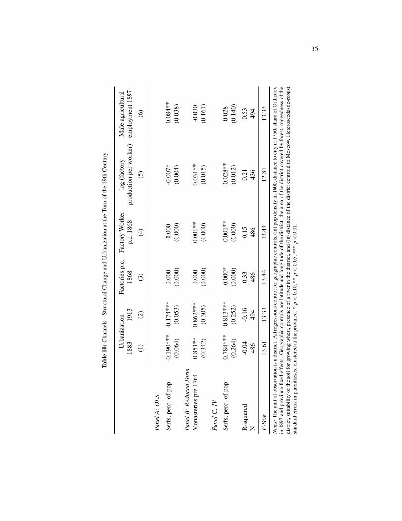
35

Tabl

e10

:Cha

nnel

s-S

truct

ural

Cha

nge

and

Urb

aniz

atio

nat

the

Turn

ofth

e19

thC

entu

ry

Urb

aniz

atio

nFa

ctor

ies

p.c.

Fact

ory

Wor

ker

log

(fac

tory

Mal

eag

ricul

tura

l18

8319

1318

68p.

c.18

68pr

oduc

tion

perw

orke

r)em

ploy

men

t189

7

(1)

(2)

(3)

(4)

(5)

(6)

Pane

lA:O

LS

Serf

s,pe

rc.o

fpop

-0.1

90**

*-0

.174

***

0.00

0-0

.000

-0.0

07*

-0.0

84**

(0.0

64)

(0.0

53)

(0.0

00)

(0.0

00)

(0.0

04)

(0.0

38)

Pane

lB:R

educ

edFo

rmM

onas

terie

spr

e17

640.

851*

*0.

862*

**0.

000

0.00

1**

0.03

1**

-0.0

30(0

.342

)(0

.305

)(0

.000

)(0

.000

)(0

.015

)(0

.161

)

Pane

lC:I

V

Serf

s,pe

rc.o

fpop

-0.7

84**

*-0

.813

***

-0.0

00*

-0.0

01**

-0.0

28**

0.02

8(0

.264

)(0

.252

)(0

.000

)(0

.000

)(0

.012

)(0

.140

)

R-s

quar

ed-0

.04

-0.1

60.

330.

150.

210.

53N

486

494

486

486

436

494

F-S

tat

13.6

113

.33

13.4

413

.44

12.8

113

.33

Not

es:

The

unit

ofob

serv

atio

nis

adi

stric

t.A

llre

gres

sion

scon

trolf

orge

ogra

phic

cont

rols

,(ln

)pop

dens

ityin

1600

,dis

tanc

eto

city

in17

50,s

hare

ofO

rthod

oxin

1897

and

prov

ince

fixed

effe

cts.

Geo

grap

hic

cont

rols

are

latit

ude

and

long

itude

ofth

edi

stric

t,th

ear

eaof

the

dist

rictc

over

edby

fore

st,r

ugge

dnes

sof

the

dist

rict,

suita

bilit

yof

the

soil

forg

row

ing

whe

at,p

rese

nce

ofa

river

inth

edi

stric

t,an

d(ln

)dis

tanc

eof

the

dist

rictc

entro

idto

Mos

cow

.Het

eros

ceda

stic

-rob

ust

stan

dard

erro

rsin

pare

nthe

ses,

clus

tere

dat

the

prov

ince

.*p<

0.10

,**

p<

0.05

,***

p<

0.01

.

36

the legacy of serfdom reduced male agricultural employment in 1897 (defined asthe primary occupation). However, this difference goes away in the IV specifi-cation. This may be due to measurement error in this variable, since it reflects awide variety of primary occupations.57 Overall, we interpret the results in Table10 as suggestive of a persistent impact of prior serfdom on subsequent structuralchange.58

4 Concluding Remarks

In this paper, we have explored whether coercive labor institutions that ex-isted for centuries in the Russian Empire generated persistent effects on eco-nomic development that lasted until today. The evidence that we marshall con-firms the adverse economic consequences to Russian serfdom that the literaturehas assumed but never definitively proven. Our study adds to a recent literaturethat has found negative long-run effects of forced labor in other contexts, de-spite the absence of religious or racial markers of past coercion in the Russiancontext. We provide evidence that the experience of serfdom generated con-straints on urbanization and structural change and fostered inequality in landownership, all of which worked to impede human capital accumulation in thelate Imperial period. These effects persisted through the Soviet period to to-day, resulting in lower city growth, infrastructure development, and, eventually,educational attainment and income levels. Thus, our results imply that early in-dustrial development and subsequent agglomeration and human capital effectscan be important channels of persistence, even over periods of dramatic socialand economic change.

The failure to develop adequate institutions to support market and politicaldevelopment has been a theme of recent research into Eastern Europe’s tran-sition since the fall of the Soviet Union (e.g. Aslund (2013)). This literaturehas generally focused on the inefficiencies generated by remnants of Soviet-era

57This measure includes males in fishing, hunting, and both modern and traditional formsof agricultural work in the numerator. By focusing on the primary occupation, it excludesvarious types of industrial or service-sector secondary occupations, which were often seasonallyimportant.

58We also explored data on the height (in mm) of military recruits in the 1870s as an addi-tional proxy for economic development in the post-emancipation period. OLS estimates (notreported here) show that recruits were significantly smaller on average when they were born inareas with high serfdom. While the IV coefficients are much larger, the coefficients are statisti-cally insignificant.

37

institutions and the difficulties in developing modern replacements. As we haveemphasized, serfdom constituted a set of dysfunctional institions with severalimplications for the subsequent development of the Soviet Union and succes-sor states. Thus, our study points to possible deeper historical roots for theinstitutional impediments that the Russian Federation and other former mem-bers of the Russian Empire currently face in their efforts at economic reformand modernization, a hypothesis that has been proposed but remains relativelyuntested.59

Many interesting questions remain open for further research. For example,one might ask how specific Imperial and Soviet policies, institutions, or eco-nomic shocks translated different experiences of serfdom into heterogeneity inoutcomes in the long run. A related area of further investigation is the role ofheterogeneity in the characteristics of serfdom (size and type of obligations, thenature of estate governance, etc.) and in the emancipation reforms for generat-ing variation in long-run outcomes.60 These and other issues constitute a richset of research questions that we hope to take up in future work.

References

Acemoglu, Daron, and Alexander Wolitzky. 2011. “The Economics of Labor Coer-cion.” Econometrica, 79(2): 555–600.

Acemoglu, Daron, and James Robinson. 2012. Why Nations Fail: The Origins ofPower, Prosperity and Poverty. Profile.

Acemoglu, Daron, Camilo García-Jimeno, and James A Robinson. 2012. “FindingEldorado: Slavery and Long-Run Development in Colombia.” Journal of Compara-tive Economics, 40(4): 534–564.

Acemoglu, Daron, Tarek A Hassan, and James A Robinson. 2011. “Social Struc-ture and Development: A Legacy of the Holocaust in Russia.” Quarterly Journal ofEconomics, 126(2).

Acharya, Avidit, Matthew Blackwell, and Maya Sen. 2013. “The Political Legacy ofAmerican Slavery.” Working paper.

Allen, Robert C. 2003. Farm to Factory: A Reinterpretation of the Soviet IndustrialRevolution. Princeton University Press.

59See Dower and Markevich (2014), Lankina (2012), and Roland (2012).60Markevich and Zhuravskaya (2015), for example, have found differences in how areas

developed immediately after 1861, depending on their specific experiences of serfdom.

38

Aslund, Anders. 2013. How Capitalism Was Built: The Transformation of Centraland Eastern Europe, Russia, the Caucasus, and Central Asia. . 2nd ed., CambridgeUniversity Press.

Bairoch, Paul, Jean Batou, and Pierre Chèvre. 1988. Population des villes eu-ropéennes de 800 à 1850: banque de données et analyse sommaire des résultats(la). Librairie Droz.

Bertocchi, Graziella, and Arcangelo Dimico. 2014. “Slavery, Education, and Inequal-ity.” European Economic Review.

Besley, Timothy, Torsten Persson, and Daniel M Sturm. 2010. “Political competi-tion, policy and growth: theory and evidence from the US.” The Review of EconomicStudies, 77(4): 1329–1352.

Bushen, A., ed. 1863. Nalichnoe naselenie Imperii za 1858 god. Vol. 2 of Statistich-eskiia tablitsy Rossiiskoi Imperii.

Dell, Melissa. 2010. “The Persistent Effects of Peru’s Mining Mita.” Econometrica,78(6): 1863–1903.

Dell, Melissa. 2012. “Path dependence in development: Evidence from the MexicanRevolution.” mimeo.

de Madariaga, Isabel. 1981. Russia in the Age of Catherine the Great. Yale UniversityPress.

Dennison, Tracy. 2011. The institutional framework of Russian serfdom. CambridgeUniversity Press.

Domar, E., and M. Machina. 1984. “On the Profitability of Russian Serfdom.” TheJournal of Economic History, 44(4): 919–955.

Domar, Evsey D. 1970. “The Causes of Slavery or Serfdom: a Hypothesis.” The Jour-nal of Economic History, 30(01): 18–32.

Dower, Paul, and Andrei Markevich. 2014. “A History of Resistance to Privatizationin Russia.” Journal of Comparative Economics, 42: 855–873.

Emmons, Terence. 1968. The Russian Landed Gentry and the Peasant Emancipationof 1861. Cambridge University Press.

Engerman, Stanley, and Kenneth Sokoloff. 1997. “Factor Endowments, Institutionsand Differential Paths of Growth among the New World Economies.” In How LatinAmerica Fell Behind. , ed. Stephen Haber. Stanford University Press, Stanford.

Fenske, James. 2013. “Does land abundance explain African institutions?” The Eco-nomic Journal, 123(573): 1363–1390.

Field, Daniel. 1976. The End of Serfdom: Nobility and Bureaucracy in Russia, 1855-1861. Harvard University Press.

39

Galor, Oded, and Omer Moav. 2006. “Das Human-Kapital: A Theory of the Demiseof the Class Structure.” The Review of Economic Studies, 73(1): 85–117.

Galor, Oded, Omer Moav, and Dietrich Vollrath. 2009. “Inequality in Landowner-ship, the Emergence of Human-Capital promoting Institutions, and the Great Diver-gence.” The Review of Economic Studies, 76(1): 143–179.

Gerschenkron, Alexander. 1966. “Agrarian Policies and Industrialization: Russia1861-1917.” In The Cambridge Economic History of Europe.

Hellie, Richard. 1982. Slavery in Russia, 1450-1725. University of Chicago Press.Hoch, Steven. 2004. “Did Russia’s Emancipated Serfs Really Pay too Much for Too

Little Land? Statistical Anomalies and Long-Tailed Distributions.” Slavic Review,63(2): 247–274.

Hoch, Steven L., and Wilson Augustine. 1979. “The Tax Censuses and the Decline ofthe Serf Population in Imperial RUssia, 1833-1858.” Slavic Review, 38(3): 403–425.

Kabuzan, V. M. 2002. Krepostnoe naselenie Rossii v XVIII v. – 50-x godakh XIX v.BLITS.

Kamenskii, Aleksandr. 1997. The Russian in the Eighteenth Century: Searching for aPlace in the World. M. E. Sharpe.

Kashchenko, Sergei. 2002. Otmena krepostnogo prava v stolichnoi gubernii. St. Pe-tersburg State University.

Khristoforov, Igor. 2011. Sud’ba Reformy: Russkoe krest’ianstvo i pravitel’stvennoipolitike do i posle otmeny krepostnogo prava (1830-1890-e gg.). Sobranie.

Kloss, Boris M. 2013. “Monasticism During the Formation of a Centralized State.”Russian Studies in History, 52(1): 5–37.

Koval’chenko, Ivan. 1967. Russkoe krepostnoe krest’ianstvo v pervoi polovine XIXveka. Moscow University Press.

Lankina, Tomila. 2012. “Unbroken Links? From Imperial Human Capital to Post-Communist Modernisation.” Europe-Asia Studies, 64(4): 623–643.

Lenin, Vladimir I. 1911. “The Peasant Reform and the Proletarian-Peasant Revolu-tion.” Collected Works, 17.

Litvak, Boris. 1972. Russkaia derevnia v reforme 1861 goda. Nauka.Markevich, Andrei, and Ekaterina Zhuravskaya. 2015. “Economic Effects of the

Abolition of Serfdom: Evidence from the Russian Empire.” Working paper.Michalopoulos, Stelios, and Elias Papaioannou. 2013. “Pre-Colonial Ethnic Institu-

tions and Contemporary African Development.” Econometrica, 81(1): 113–152.Moon, David. 1999. The Russian Peasantry 1600-1930: The World the Peasants Made.

Longman.

40

Nafziger, Steven. 2011. “Did Ivan’s Vote Matter? The Political Economy of LocalDemocracy in Tsarist Russia.” European Review of Economic History, 15: 393–441.

Nafziger, Steven. 2012a. “The Political Economy of Primary Education in Tsarist Rus-sia.” Working paper.

Nafziger, Steven. 2012b. “Serfdom, Emancipation, and Off-Farm Labour Mobility inTsarist Russia.” Economic History of Developing Regions, 27(1): 1–37.

Nafziger, Steven. 2013. “Russian Serfdom, Emancipation, and Land Inequality: NewEvidence.” Working paper.

Nunn, Nathan. 2008a. “The Long-Term Effects of Africa’s Slave Trades.” The Quar-terly Journal of Economics, 123(1): 139–176.

Nunn, Nathan. 2008b. “Slavery, Inequality, and Economic Development in the Amer-icas.” Institutions and Economic Performance.

Nunn, Nathan. 2012. “Culture and the historical process.” Economic History of Devel-oping Regions, 27(sup1): S108–S126.

Nunn, Nathan. 2013. “Historical Development.” Handbook of Economic Growth,2: 347.

Ostrowski, Donald. 1986. “Church Polemics and Monastic Land Acquisition inSixteenth-Century Muscovy.” Slavonic and East European Review, 64(3): 355–379.

Roland, Gerard. 2012. “The Long Run Weight of Communism or the Weight of LongRun History?” In Economies in Transition: The Long-Run View. , ed. Gerard Roland,153–171. Palgrave Macmillan.

Romaniello, Matthew P. 2000. “Controlling the Frontier: Monasteries and Infrastruc-ture in the Volga Region, 1552-1682.” Central Asian Survey, 19(3/4): 429–443.

Troinitskii, N. A. 1982 (1861). The Serf Population in Russia According to the 10thNational Census. Oriental Research Partners.

Weickhardt, George G. 2012. “Muscovite Law on Monasteries.” Russian History,39: 13–41.

Wirtschafter, Elise. 1997. Social Identity in Imperial Russia. Northern Illinois Univer-sity Press.

Zaidi, Salman, et al. 2009. Satisfaction with life and service delivery in Eastern Europeand the former Soviet Union: some insights from the 2006 life in transition survey.World Bank Publications.

Zakharova, Larissa. 1982. “K posledstviiam sekuliarizatsii tserkovnykh zemel’ vRossii.” Voprosy istorii, 12: 165–167.

Zinchenko, A. L. 1985. “Reforma gosudarstvennoi derevni i sekuliarizatsiia v zapad-nykh guberniiakh Rossiiskoi imperii.” Istoricheskie zapiski, 112: 98–125.

41

Zverinskii, V. V., ed. 2005 (1897). Monastyri zakrytye do Tsarstvovaniia ImperatritsyEkaterinay II. Dmitrii Bulanin.

Online Appendix forLong-Run Consequences of Labor Coercion:

Evidence from Russian Serfdom

Johannes C. Buggle⇤ Steven Nafziger†

A Data Appendix and Supplementary Tables and Figures

This appendix accompanies the paper “Long-Run Consequences of Labor Coercion: Evi-dence from Russian Serfdom” by Johannes C. Buggle and Steven Nafziger. Section A.1 de-scribes the data and its sources. Sections A.2 contains additional tables and results mentionedin the paper, and section A.3 contains supplementary figures.

A.1 Data Description and Sources

• Serfdom Data: The main explanatory variable, Serfs, perc. of pop, is constructed usingthe sum of total male and female serfs in 1858 per district (taken from Troinitskii (1982(1861)), divided by district population in 1858 (taken from Bushen (1863)). The lattersource also allows us to construct a measure of population density for 1858.

• Geographic Controls:Longitude and latitude information based on own calculations at the district’s centroidusing ArcGIS.Ln Distance to Moscow gives log of the straight line distance in kilometers from thecentroid of each historical district to Moscow (own calculation using ArcGIS).Suitability of the soil for low-input rain-fed wheat, oat, rye and barley, as well asruggedness and forest cover are taken from the FAO-GAEZ database.The presence of a river (0/1) is calculated using a digitized map of rivers pro-duced by the Alterra Centre for Geo-Information (accessed through http://climate-adapt.eea.europa.eu/geonetwork/srv/en/main.home).Ln Population Density in 1600 is constructed using population density data

⇤Department of Economics, Sciences Po, 27 Rue des Saints-Peres, 75007 Paris, France. jo-hannes.buggle@sciencespo.fr

†Department of Economics, Williams College, Schapiro Hall, 24 Hopkins Hall Dr., Williamstown, MA 01267.snafzige@williams.edu

from the HYDE 3.1 database which provides population density estimatesfrom 10000 BC to AD 2000 for every hundred years, and every ten yearsfrom 1700 onsward (Klein Goldewijk et al., 2011) (downloadable fromhttp://themasites.pbl.nl/tridion/en/themasites/hyde/download/index-2.html).The distance to nearest city is constructed by the distance in kilometers from the district’scentroid to the closest city in 1750, as reported in the data by Bairoch, Batou and Chèvre(1988) using ArcGIS.Ln Population Density in 2000 is based on the Gridded Population of the World (GPW),v3, data.

• Monasteries prior 1764: Total number of orthodox monasteries per district prior to 1764,obtained from Zverinskii (2005 (1897)).

• Log Equivalent Expenditure Per Capita comes from questions asking “Approximatelyhow much does your household spend on each of these items per month?” a) Food,beverages and tobacco, b) Utilities (electricity, water, gas, heating, fixed line phone.), c)Transportation (public transportation, fuel for car) and “And approximately how much didyour household spend on each of these items during the past 12 months?” a) Education(including tuition, books, kindergarten expenses), b) Health (including medicines andhealth insurance), c) Clothing and footwear, d) Durable goods (e.g. furniture, householdappliances. TV, car, etc). Expressed in US Dollars and adjusted by household size. Sourceis Life in Transition Survey, wave 2006.

• Asset ownership: Question asks “Do you or anyone in your household own any of thefollowing?” We construct a principle component out of ownership of a car, a secondresidence, a mobile phone, or a computer. Source is Life in Transition Survey, wave 2006and 2010.

• Access to Public Goods: Question asks “Do you have access to [UTILITY] in thisdwelling?” and UTILITY are different type of public goods, such as water, central heat-ing, telephone, public sewage system. Source is Life in Transition Survey, wave 2006 and2010.

• Base and household controls: Household size, share of male, share of persons aged0-18, share of persons aged 60+, religious denomination of the respondent, rural/urbansampling village, survey round. Source is Life in Transition Survey, wave 2006 and 2010.

• Education: Secondary equals 1 if the educational level of the respondent is either sec-ondary education, professional education, tertiary education or postgraduate education, 0otherwise. Above secondary education equals 1 if the educational level of the respondentis either professional education, tertiary education or postgraduate education, 0 other-wise. We also use the question “In your opinion, which of these fields should the first

2

priority for extra (government) investment?” to construct an indicator variable equal 1 ifthe respondent mentions education.

• Attitudes:Equal incomes vs inequality: Question asks “Now I’d like you to tell me your views onvarious issues. How would you place your views on this scale? 1 means you agree com-pletely with the statement on the left; 10 means you agree completely with the statementon the right; and if your views fall somewhere in between, you can choose any number inbetween: Incomes should be made more equal (1) vs We need larger income differencesas incentives for individual effort (10)”.Reduce Inequality: Question asks “To what extent do you agree with the following state-ments: The gap between the rich and the poor today in this country should be reduced”and respondents can strongly agree (1), agree (2), neither agree nor disagree (3), disagree(4) or strongly disagree (5).Poor: ... : Question asks “In your opinion, what is the main reason why there are somepeople in need in our country today? Because they have been unlucky - Because of lazi-ness and lack of willpower - Because of injustice in our society - It is an inevitable partof modern life” We create dummies that takes on the value 1 if the respondent mentionedone of the choices.Demonstrated/Striked/Joined Party: Question asks “How likely are you to... attend alawful demonstration - participate in a strike - join a political party” and respondents cananswer “have done (3) - might do (2) - would never do (1)”Pref Market Economy: Question asks “With which one of the following statements doyou agree most? A market economy is preferable to any other form of economic system- Under some circumstances, a planned economy may be preferable to a market econ-omy - For people like me, it does not matter whether the economic system is organizedas a market economy or as a planned economy” The variable takes on the value 1 if therespondent states that “A market economy is preferable to any other form of economicsystem ” and 0 otherwise.Pref Democracy: Question asks “With which one of the following statements do youagree most? Democracy is preferable to any other form of political system - Under somecircumstances, an authoritarian government may be preferable to a democratic one - Forpeople like me, it does not matter whether a government is democratic or authoritarian”The variable takes on the value 1 if the respondent states that “Democracy is preferableto any other form of political system ” and 0 otherwise.

• City Population 1929 - 1989: Data measuring the populations of Russian cities from1929 to 1989 is taken from Acemoglu, Hassan and Robinson (2011).

• Road and Railway Density in the Countries of the former Soviet Union: Road

3

and Railway densities in 1996 are constructed using digitized maps provided by theCoal Quality and Resources of the Former Soviet Union project of the U.S. Geologi-cal Survey (Brownfield et al. 2001), accessed via http://pubs.usgs.gov/of/2001/ofr-01-104/fsucoal/html/data1.htm.

• Historical Outcomes: We drew on a variety of sources to construct other historical out-come measures to investigate the mechanisms behind the persistent impact of serfdom.Male literacy in 1897 is defined for rural residents in their 20s from data reported inTroinitskii (1905). That source also provides the share of the adult male population withagriculture as the primary occupation. Rural enrollment rates for 1880 and 1894 are de-fined with both numerators and denominators taken from Tsentraf’nyi statisticheckikhkomitet, Ministerstvo vnutrennykh del (1884) and Fal’bork and Charnoluskii (1900-1905), respectively – see Nafziger (2012) for more information. Fal’bork and Charno-luskii (1900-1905) also provide the number of formally recognized primary schoolsby district in 1856. The urbanization rate in 1913 is derived from Tsentraf’nyi statis-ticheckikh komitet, Ministerstvo vnutrennykh del (1914). The land Gini (both types),the percentage of land owned by the nobility or in communal tenure, and the amount ofland possessed per peasant household, all defined in 1905, are from Tsentraf’nyi statis-ticheckikh komitet, Ministerstvo vnutrennykh del (1906), with additional details providedin Nafziger (2013). Finally, information on factory production and employment in 1868is compiled from Tsentraf’nyi statisticheckikh komitet, Ministerstvo vnutrennykh del(1872).

• Night-Time Luminosity: We use the log of average luminosity at night mea-sured as “Average Visible, Stable Lights, and Cloud Free Coverage” for theyear 2008. The data is taken from the National Geophysical Data Center(http://ngdc.noaa.gov/eog/dmsp/downloadV4composites.html).

4

A.2 Supplementary Tables

Table A1: Summary Statistics

Mean Sd Obs

Serfdom and MonasteriesSerfs, perc. of pop 38.52 25.01 494Monasteries pre 1764 1.61 3.12 494

Control Variables at the District-LevelLongitude 37.10 8.58 494Latitude 54.10 3.84 494Forest Cover 36.05 23.57 494Ruggedness 91.29 4.91 494Wheat Suitability 6621.15 2184.24 494River (0-1) 0.55 0.50 494Distance to Moscow (ln) 6.28 0.66 494Oat Suitability 6070.91 2303.28 494Rye Suitability 6000.32 2259.95 494Barley Suitability 6067.84 2335.83 494(ln) Population Density 1600 1.13 0.95 494Distance to City in 1750 94.86 83.31 494Share Orthodox 1897 82.98 25.49 494

Additional Outcomes at the District-LevelIntermediate OutcomesSchools before 1856 (p. thousand inhabitants) 0.05 0.13 489log rural enrollment rate of boys in 1880 2.48 0.56 492log rural enrollment rate of girls 1880 0.30 1.20 492log rural enrollment rate of boys and girls in 1894 -1.99 0.47 494log(teacher wage 1910) 5.77 0.20 492Perc. Land owned by Nobles, 1905 20.86 14.04 494Peasant Land per HH, 1905 14.87 15.55 494Land Gini 1905 0.49 0.16 470Land Gini 1905 (only private land) 0.77 0.14 479Urbanization 1833 10.33 12.69 486Urbanization 1913 10.09 12.15 494Factories p.c. 1868 0.00 0.00 486Factory Worker p.c. 1868 0.01 0.06 486

5

Table A1: Summary Statistics (continued)

Mean Sd Obs

log(factory production per worker) 6.09 0.93 436Male agricultural employment 1897 71.58 14.81 494Road Density Soviet Union 1.67 1.22 494Rail Density Soviet Union 2.08 1.90 494

Contemporary OutcomesLn Luminosity 2008 0.57 1.01 494

Contemporaneous Survey Outcomes (LiTS)Serfs, perc. of pop 23.90 24.89 12831

Latitude PSU 53.66 4.28 12831Longitude PSU 29.27 6.99 12831

Economic and Public GoodsLog Equivalent Expenditure Per Capita 4.96 0.85 5605Household Durable Assets (Principal Component) 0.01 1.34 12826Public Goods (Principal Component) 0.03 1.55 5897

EducationAt least secondary education 0.71 0.45 12831Above secondary education 0.56 0.50 12830Mentioned education first gov priority 0.23 0.42 12829

Cultural AttitudesEconomic inequality 4.74 2.97 6558Reduce Inequality 4.04 1.00 12216Poor: society unjust 0.42 0.49 12830Poor: unlucky 0.08 0.27 12830Poor: lazy 0.26 0.44 12830Poor: inevitable 0.17 0.38 12830Demonstrated 1.38 0.59 11834Striked 1.30 0.51 11834Joined Party 1.18 0.45 11834Pref Market Economy 0.38 0.49 11573Pref Democracy 0.49 0.50 11663

See the Data Appendix for variable definitions and sources.

6

Individual Level Regressions with Asset Ownership as Dependent Variable We find sim-ilar results to those in Table 4 of the main paper when using the principal component of durableassets owned by the household as measure of economic well-being today. These results arereported in Table A2. Both the OLS estimates in Panel A, as well as the IV coefficients inPanel C point towards a significantly lower level of asset ownership among households living informer serf areas. A one standard deviation increase in serfdom reduces contemporaneous assetownership by up to 0.08 of a standard deviation in the OLS estimations, and 0.3 of a standarddeviation in the IV estimations.

Table A2: Contemporary Household Assets

Household Assets (Principal Component)

(1) (2) (3) (4) (5)

Panel A: OLS

Serf, perc. of pop (x100) -0.300* -0.409** -0.408** -0.241 -0.221(0.182) (0.185) (0.194) (0.189) (0.204)

Panel B: Reduced Form

Monasteries pre 1764 0.020** 0.029*** 0.028*** 0.027*** 0.026***(0.009) (0.010) (0.010) (0.010) (0.010)

Panel C: IV

Serf, perc. of pop (x100) -1.289** -1.699*** -1.926*** -1.642*** -1.890**(0.580) (0.586) (0.730) (0.595) (0.754)

R-squared 0.39 0.39 0.39 0.39 0.39N 12836 12836 12836 12836 12836

F-stat 169.82 115.01 59.34 123.05 58.72

Base and Household Controls Yes Yes Yes Yes YesGeographic Controls No Yes Yes Yes Yes(ln) Pop Density 1600 No No Yes No YesDistance City 1750 No No Yes No YesShare Orthodox 1897 No No No Yes YesFE Province Province Province Province ProvinceCluster PSU PSU PSU PSU PSU

Notes: The unit of observation is the individual. The dependent variable is principal component of householdasset ownership (car, second residence, mobile phone, computer), taken from LiTS waves 2006 and 2010. Allregressions control for a set of base controls (religious denomination of the respondent, LiTS survey wave and anindicator whether the PSU is rural or urban) and household controls (household size, share of household membersaged 0-18, share of household members aged 60+, share of male household members). Geographic controls arelatitude and longitude of the PSU, area of the district covered by forest, ruggedness of the district, suitability ofthe soil for growing wheat, presence of a river in the district, and (ln) distance of the district centroid to Moscow.Heteroscedastic-robust standard errors in parentheses, clustered at the primary sampling unit. * p < 0.10, **p < 0.05, *** p < 0.01.

7

Additional Robustness of the OLS Regressions Using Household Expenditure Table A3reports robustness of the OLS estimations using household expenditure as dependent variablewith country fixed effects instead of province fixed effects in Panel A, and controlling for urban-ization in 1883 in Panel B. While the rate of urbanization has a positive effect on expenditurein Columns 1 and 2, once we include controls for historical development (population densityin 1600 and distance to city in 1750), urbanization becomes insignificant (Column 3 and 4),giving additional credibility that the historical measures are very good proxies for long-termdevelopment. As Columns (1) to (3) show, serfdom is significantly associated with householdexpenditure conditional on the rate of urbanization.

Table A3: Additional Robustness

Log Equivalent Expenditure Per Capita

(1) (2) (3) (4)

Panel A: Country Fixed Effects

Serf, perc. of pop (x100) -0.286*** -0.557*** -0.466*** -0.376***(0.108) (0.110) (0.113) (0.115)

R-squared 0.41 0.42 0.43 0.43N 5605 5605 5605 5605Base and Household Controls Yes Yes Yes YesGeographic Controls No Yes Yes Yes(ln) Pop Density 1600 No No Yes YesDistance City 1750 No No Yes YesReligion 1897 No No No YesFE Country Country Country CountryCluster PSU PSU PSU PSU

Panel B: Urbanization 1883

Serf, perc. of pop (x100) -0.458*** -0.557*** -0.398** -0.269(0.155) (0.171) (0.180) (0.186)

Urbanization 1883 0.317** 0.306** 0.125 0.165(0.131) (0.127) (0.155) (0.191)

R-squared 0.44 0.44 0.45 0.45N 5368 5368 5368 5368Base and Household Controls Yes Yes Yes YesGeographic Controls No Yes Yes Yes(ln) Pop Density 1600 No No Yes YesDistance City 1750 No No Yes YesShare Orthodox 1897 No No No YesFE Province Province Province ProvinceCluster PSU PSU PSU PSU

Notes: The unit of observation is the individual. The dependent variable is Log Equivalent Expen-diture Per Capita, taken from LiTS wave 2006. All regressions control for a set of base controls(religious denomination of the respondent, LiTS survey wave and an indicator whether the PSU isrural or urban) and household controls (household size, share of household members aged 0-18, shareof household members aged 60+, share of male household members). Geographic controls are latitudeand longitude of the PSU, area of the district covered by forest, ruggedness of the district, suitability ofthe soil for growing wheat, presence of a river in the district, and (ln) distance of the district centroidto Moscow. Heteroscedastic-robust standard errors in parentheses, clustered at the primary samplingunit. * p < 0.10, ** p < 0.05, *** p < 0.01.

8

Using Night-Time Luminosity as Outcome Variable We investigate the effects of histori-cal serfdom on contemporary development using the log of night-time light intensity in 2008,measured within the historical districts, as our dependent variable. Night-time luminosity havebeen increasingly utilized as a proxy for economic development of sub-national units in theabsence of other aggregate economic measures (e.g. Henderson, Storeygard and Weil (2012)).Table A4 reports the results for the OLS, reduced form, and IV regressions. Overall, areas withhigher shares of serfdom display lower levels of luminosity at night today, in both OLS and IVspecifications, conditioning on province fixed effects and geographic controls (Column 1). Theestimated coefficients stay relatively stable when additional controls are subsequently includedin Columns 2 and 3. The overall magnitudes of the effects are economically meaningful, but,as in our expenditure results, they vary substantially between a 20% reduction in the OLS anda 75% reduction in night light intensity in the IV specification for a one standard deviationchange in serfdom.1 As an alternative indicator for long run development, we can use log popu-lation density in 2000 as outcome variable, conditioning on log population density in 1600. AsColumn 4 shows, serfdom is associated with significantly lower population density in the year2000, and the magnitudes of the coefficients vary between a 20% (OLS) and 75% (IV) decreasefor a one standard deviation change in the incidence of serfdom.

The estimated coefficients stay relatively stable when additional controls are subsequentlyincluded in Columns 2 and 3. The overall magnitudes of the effects are economically mean-ingful, but, as in our expenditure results, they vary substantially between a 20% reduction inthe OLS and a 75% reduction in night light intensity in the IV specification for a one standarddeviation change in serfdom.2 As an alternative indicator for long run development, we can uselog population density in 2000 as outcome variable, conditioning on log population density in1600. As Column 4 shows, serfdom is associated with significantly lower population density inthe year 2000, and the magnitudes of the coefficients vary between a 20% (OLS) and 75% (IV)decrease for a one standard deviation change in the incidence of serfdom.

1A 75% reduction in luminosity might seem very large, but is not unreasonable compared to magnitudes inother papers studying long-run persistence using night-time lights. Michalopoulos and Papaioannou (2013) forexample report that pre-colonial ethnic political centralization increases luminosity by between 30 and 70 % inAfrica.

2A 75% reduction in luminosity might seem very large, but is not unreasonable compared to magnitudes inother papers studying long-run persistence using night-time lights. Michalopoulos and Papaioannou (2013) forexample report that pre-colonial ethnic political centralization increases luminosity by between 30 and 70 % inAfrica.

9

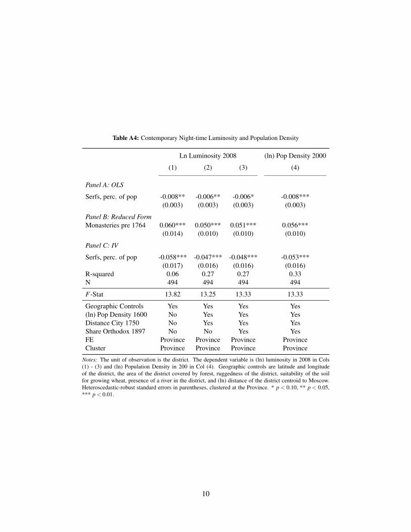
Table A4: Contemporary Night-time Luminosity and Population Density

Ln Luminosity 2008 (ln) Pop Density 2000

(1) (2) (3) (4)

Panel A: OLS

Serfs, perc. of pop -0.008** -0.006** -0.006* -0.008***(0.003) (0.003) (0.003) (0.003)

Panel B: Reduced FormMonasteries pre 1764 0.060*** 0.050*** 0.051*** 0.056***

(0.014) (0.010) (0.010) (0.010)

Panel C: IV

Serfs, perc. of pop -0.058*** -0.047*** -0.048*** -0.053***(0.017) (0.016) (0.016) (0.016)

R-squared 0.06 0.27 0.27 0.33N 494 494 494 494

F-Stat 13.82 13.25 13.33 13.33

Geographic Controls Yes Yes Yes Yes(ln) Pop Density 1600 No Yes Yes YesDistance City 1750 No Yes Yes YesShare Orthodox 1897 No No Yes YesFE Province Province Province ProvinceCluster Province Province Province Province

Notes: The unit of observation is the district. The dependent variable is (ln) luminosity in 2008 in Cols(1) - (3) and (ln) Population Density in 200 in Col (4). Geographic controls are latitude and longitudeof the district, the area of the district covered by forest, ruggedness of the district, suitability of the soilfor growing wheat, presence of a river in the district, and (ln) distance of the district centroid to Moscow.Heteroscedastic-robust standard errors in parentheses, clustered at the Province. * p < 0.10, ** p < 0.05,*** p < 0.01.

10

Demand for Education Table A5 investigates differences in the demand for education. Thedependent variable comes from the LiTS question “In your opinion, which of these fields shouldthe first priority for extra (government) investment?” and equals 1 if the respondent mentionseducation, 0 otherwise.

Table A5: Channels - Demand for Education

Education Government Priority

(1) (2)

Panel A: OLS

Serfs, perc. of pop (x100) -0.085 -0.102(0.059) (0.062)

Panel B: Reduced Form

Monasteries pre 1764 0.003 0.004*(0.002) (0.002)

Panel C: IVSerfs, perc. of pop (x100) -0.200 -0.299*

(0.134) (0.177)

R-squared 0.04 0.04N 12829 12829

F-stat 115.12 59.21

Base and Household Controls Yes YesGeographic Controls Yes Yes(ln) Pop Density 1600 No YesDistance City 1750 No YesShare Orthodox 1897 No YesFE Province ProvinceCluster PSU PSU

Notes: The unit of observation is the individual. All regressions control for a setof base controls (religious denomination of the respondent, LiTS survey waveand an indicator whether the PSU is rural or urban) and household controls(household size, share of household members aged 0-18, share of householdmembers aged 60+, share of male household members). Geographic controls arelatitude and longitude of the district, the area of the district covered by forest,ruggedness of the district, suitability of the soil for growing wheat, presenceof a river in the district, and (ln) distance of the district centroid to Moscow.Heteroscedastic-robust standard errors in parentheses, clustered at the principalsampling unit. * p < 0.10, ** p < 0.05, *** p < 0.01.

11

Cultural Attitudes Did economic exploitation over several centuries shape peoples beliefsand attitudes, perhaps fostering a “culture of serfdom,” with persistent implications for eco-nomic development? Several recent studies have documented that institutions can impact cul-tural norms in the long-run (for an overview see Nunn (2012)), which can persist over gener-ations. Moreover, it is possible that various institutional restrictions, social and economic in-equality, or persistent limitations on urban development under and after serfdom generated long-lasting norms and beliefs that undermined income growth in modern post-Soviet economies.

To explore this possibility, we rely on survey responses regarding various beliefs, as elicitedin the 2006 and 2010 rounds of LiTS. Our results are presented in Table A6. We consider at-titudes about inequality and redistribution (Columns 1 and 2), a number of questions that askabout the beliefs regarding the reasons for poverty (Column 3 to 6), political action (Column7 to 9), as well as preferences for a market economy (Column 10) or democracy (Column 11).Respondents seem to be more likely to prefer less income inequality: the OLS and IV estimatesare significant for preferences for economic equality (Column 1), but there is no differential in-terest in having government reduce inequality (Column 2). Our results suggest that individualsin formerly high serf areas think, on average, that the poor are poor because they are unlucky.They are less likely to mention laziness as a reason for poverty in the OLS model (column 5), butsurprisingly the sign of the coefficient flips in the IV specification (as it does with respect to theinevitability of poverty). 3 We find no evidence that individuals living in areas with historicallygreater intensity of serfdom were more likely to engage in political actions, such as demonstra-tions (Column 7), attending a strike (Column 8) (although the OLS coefficient is marginallysignificant), or joining a political party (Column 9).4 Finally, preferences for a market economy(versus a planned economy) or for democracy (versus autocracy) are not statistically differentbetween areas with a greater or lesser history of serfdom.5

While cultural channels have been emphasized in the literature on persistent effects of pastlabor coercion (i.e. Nunn and Wantchekon (2011)), we find only limited support for this in theRussian and former Soviet case. Unlike societies with legacies of racially delineated slavery, asthe US South, the absence of significant racial or religious differences between former serfs andthe rest of the population may have limited any such cultural distinctiveness in the subsequentdecades.

3While these results deserve further exploration, for now we simply note that there seems to be systematicdifferences in how residents of former serf areas see the roots of poverty today. This could be based in cultural dif-ferences, or it could reflect more fundamental structural or institutional factors that have accompanied the relativelypoorer economic conditions in such areas.

4This contrasts with the results in Dower et al. (2015), who find that emancipation generated considerablecollective action in the form of peasant unrest in the early 1860s among the newly freed former serfs. However,given the legacy of political repression in the late Imperial period and under the Soviet Union, perhaps this is notsurprising.

5We also explored measures of interpersonal trust and trust in governmental institutions as outcomes but didnot find any significant differences. These results are available upon request.

12

Tabl

eA

6:C

hann

els

-Cul

tura

lAtti

tude

san

dPr

efer

ence

s

Econ

omic

ineq

ualit

yG

ovts

houl

dre

duce

ineq

ualit

yPo

verty

bcso

ciet

yun

just

Pove

rtybc

bad

luck

Pove

rtybc

lazy

Pove

rtyin

evita

ble

Dem

onst

rate

dSt

riked

Join

edPa

rtyPr

efM

arke

tEco

nom

yPr

efD

emoc

racy

(1)

(2)

(3)

(4)

(5)

(6)

(7)

(8)

(9)

(10)

(11)

Pane

lA:O

LS

Serf

s,pe

rc.o

fpop

(x10

0)-1

.764

*0.

061

-0.1

290.

075*

*-0

.034

0.00

80.

147

0.17

4*0.

065

-0.0

80-0

.035

(0.9

76)

(0.1

94)

(0.0

83)

(0.0

35)

(0.0

67)

(0.0

62)

(0.1

06)

(0.0

92)

(0.0

67)

(0.0

89)

(0.1

05)

Pane

lB:R

educ

edFo

rm

Mon

aste

ries

pre

1764

0.09

0*0.

021

0.00

3-0

.001

-0.0

07**

0.00

3-0

.001

-0.0

02-0

.004

-0.0

05-0

.002

(0.0

53)

(0.0

13)

(0.0

04)

(0.0

02)

(0.0

03)

(0.0

03)

(0.0

06)

(0.0

04)

(0.0

04)

(0.0

05)

(0.0

06)

Pane

lC:I

VSe

rfs,

perc

.ofp

op(x

100)

-5.4

74*

-1.5

19-0

.207

0.08

50.

512*

*-0

.185

0.03

60.

122

0.31

20.

364

0.16

7(3

.298

)(0

.991

)(0

.285

)(0

.116

)(0

.241

)(0

.194

)(0

.385

)(0

.243

)(0

.263

)(0

.398

)(0

.447

)

R-s

quar

ed-0

.01

-0.0

20.

000.

00-0

.01

-0.0

00.

000.

00-0

.00

-0.0

1-0

.00

N65

5812

216

1283

012

830

1283

012

830

1183

411

834

1183

411

573

1166

3

F-s

tat

56.3

261

.33

59.1

959

.19

59.1

959

.19

67.0

467

.04

67.0

458

.02

56.9

1

Not

es:

The

unit

ofob

serv

atio

nis

the

indi

vidu

al.A

llre

gres

sion

sco

ntro

lfor

the

age,

age

squa

red

and

gend

erof

the

resp

onde

nt,a

sw

ella

sa

seto

fbas

eco

ntro

ls(r

elig

ious

deno

min

atio

nof

the

resp

onde

nt,L

iTS

surv

eyw

ave

and

anin

dica

torw

heth

erth

ePS

Uis

rura

loru

rban

)and

hous

ehol

dco

ntro

ls(h

ouse

hold

size

,sha

reof

hous

ehol

dm

embe

rsag

ed0-

18,s

hare

ofho

useh

old

mem

bers

aged

60+,

shar

eof

mal

eho

useh

old

mem

bers

).G

eogr

aphi

cco

ntro

lsar

ela

titud

ean

dlo

ngitu

deof

the

dist

rict,

the

area

ofth

edi

stric

tcov

ered

byfo

rest

,rug

gedn

esso

fthe

dist

rict,

suita

bilit

yof

the

soil

forg

row

ing

whe

at,p

rese

nce

ofa

river

inth

edi

stric

t,an

d(ln

)dis

tanc

eof

the

dist

rictc

entro

idto

Mos

cow

.All

regr

essi

ons

incl

ude

prov

ince

fixed

effe

cts.

Het

eros

ceda

stic

-rob

usts

tand

ard

erro

rsin

pare

nthe

ses,

clus

tere

dat

the

prim

ary

sam

plin

gun

it.*

p<

0.10

,**

p<

0.05

,***

p<

0.01

.

13

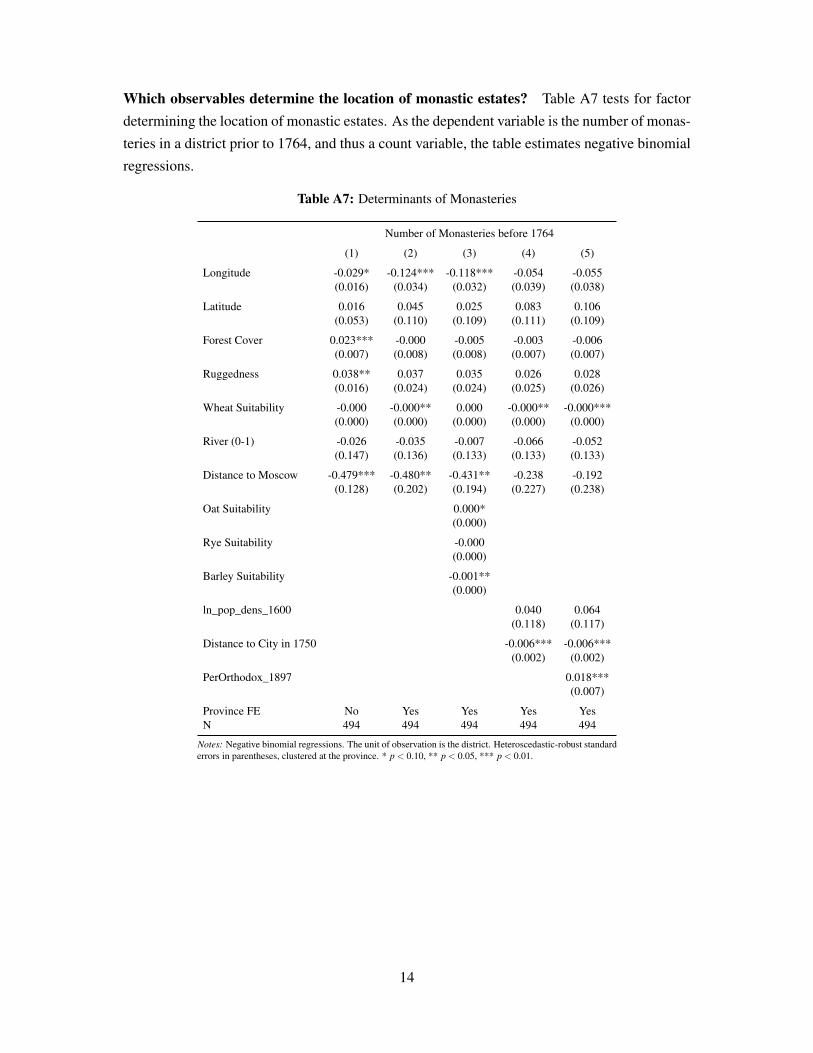
Which observables determine the location of monastic estates? Table A7 tests for factordetermining the location of monastic estates. As the dependent variable is the number of monas-teries in a district prior to 1764, and thus a count variable, the table estimates negative binomialregressions.

Table A7: Determinants of Monasteries

Number of Monasteries before 1764

(1) (2) (3) (4) (5)

Longitude -0.029* -0.124*** -0.118*** -0.054 -0.055(0.016) (0.034) (0.032) (0.039) (0.038)

Latitude 0.016 0.045 0.025 0.083 0.106(0.053) (0.110) (0.109) (0.111) (0.109)

Forest Cover 0.023*** -0.000 -0.005 -0.003 -0.006(0.007) (0.008) (0.008) (0.007) (0.007)

Ruggedness 0.038** 0.037 0.035 0.026 0.028(0.016) (0.024) (0.024) (0.025) (0.026)

Wheat Suitability -0.000 -0.000** 0.000 -0.000** -0.000***(0.000) (0.000) (0.000) (0.000) (0.000)

River (0-1) -0.026 -0.035 -0.007 -0.066 -0.052(0.147) (0.136) (0.133) (0.133) (0.133)

Distance to Moscow -0.479*** -0.480** -0.431** -0.238 -0.192(0.128) (0.202) (0.194) (0.227) (0.238)

Oat Suitability 0.000*(0.000)

Rye Suitability -0.000(0.000)

Barley Suitability -0.001**(0.000)

ln_pop_dens_1600 0.040 0.064(0.118) (0.117)

Distance to City in 1750 -0.006*** -0.006***(0.002) (0.002)

PerOrthodox_1897 0.018***(0.007)

Province FE No Yes Yes Yes YesN 494 494 494 494 494

Notes: Negative binomial regressions. The unit of observation is the district. Heteroscedastic-robust standarderrors in parentheses, clustered at the province. * p < 0.10, ** p < 0.05, *** p < 0.01.

14

A.3 Supplementary Figures

Figure A1: Distribution of Serfs as Share of Population, c. 1858. N = 495.

15

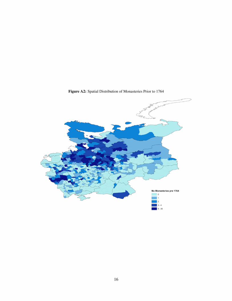
Figure A2: Spatial Distribution of Monasteries Prior to 1764

16

Figure A3: Location of LiTS Primary Sampling Units (PSU)

17

Figure A4: Avg City Population 1750-1989 and below/above Median Serfdom

18

References

Acemoglu, Daron, Tarek A Hassan, and James A Robinson. 2011. “Social Structure and Development: ALegacy of the Holocaust in Russia.” Quarterly Journal of Economics, 126(2).

Bairoch, Paul, Jean Batou, and Pierre Chèvre. 1988. Population des villes européennes de 800 à 1850: banquede données et analyse sommaire des résultats (la). Librairie Droz.

Bushen, A., ed. 1863. Nalichnoe naselenie Imperii za 1858 god. Vol. 2 of Statisticheskiia tablitsy RossiiskoiImperii.

Dower, Paul, Evgeny Finkel, Scott Gehlbach, and Steven Nafziger. 2015. “Collective Action and Representationin Autocracies: Evidence from Russia’s Great Reforms.” mimeo.

Fal’bork, G., and V. Charnoluskii, ed. 1900-1905. Nachal’noe narodnoe obrazovanie v Rossii. ImperatorskoevolÊznoe ekonomicheskoe obshchestvo.

Henderson, J Vernon, Adam Storeygard, and David N Weil. 2012. “Measuring economic growth from outerspace.” American Economic Review, 102(2): 994–1028.

Klein Goldewijk, Kees, Arthur Beusen, Gerard Van Drecht, and Martine De Vos. 2011. “The HYDE 3.1 spa-tially explicit database of human-induced global land-use change over the past 12,000 years.” Global Ecologyand Biogeography, 20(1): 73–86.

Michalopoulos, Stelios, and Elias Papaioannou. 2013. “Pre-Colonial Ethnic Institutions and ContemporaryAfrican Development.” Econometrica, 81(1): 113–152.

Nafziger, Steven. 2012. “The Political Economy of Primary Education in Tsarist Russia.” Working paper.

Nafziger, Steven. 2013. “Russian Serfdom, Emancipation, and Land Inequality: New Evidence.” Working paper.

Nunn, Nathan. 2012. “Culture and the historical process.” Economic History of Developing Regions,27(sup1): S108–S126.

Nunn, Nathan, and Leonard Wantchekon. 2011. “The Slave Trade and the Origins of Mistrust in Africa.”American Economic Review, 101(7): 3221–52.

Troinitskii, N. A. 1982 (1861). The Serf Population in Russia According to the 10th National Census. OrientalResearch Partners.

Troinitskii, N. A., ed. 1905. Pervaia vseobshchaia perepis’ naseleniia Rossiiskoi Imperii, 1897 g. Vol. Multiple,Central Statistical Committee, Ministry of the Interior.

Tsentraf’nyi statisticheckikh komitet, Ministerstvo vnutrennykh del. 1872. Statisticheskii Vremennik Rossi-iskoi Imperii. Vol. 6 of II.

Tsentraf’nyi statisticheckikh komitet, Ministerstvo vnutrennykh del. 1884. Sel’skiia uchilishcha v EvropeiskoiRossii i Privislianskikh guberniiakh. Vol. 1 of Statisticheskii vremennik Rossiiskoi imperii (Series III).

Tsentraf’nyi statisticheckikh komitet, Ministerstvo vnutrennykh del. 1906. Statistika zemliavladeniia 1905 g.Vol. Multiple.

Tsentraf’nyi statisticheckikh komitet, Ministerstvo vnutrennykh del. 1914. Statisticheskii ezhegodnik Rossii1913 g.

Zverinskii, V. V., ed. 2005 (1897). Monastyri zakrytye do Tsarstvovaniia Imperatritsy Ekaterinay II. DmitriiBulanin.

19