INSTITUTE OF DEVELOPING ECONOMIES

IDE Discussion Papers are preliminary materials circulated to stimulate discussions and critical comments

IDE DISCUSSION PAPER No. 274

Myopic or farsighted: Bilateral Trade Agreements among three symmetric countries Kenmei TSUBOTA* and Yujiro KAWASAKI**

Keywords: Endogenous network formation, Bilateral trade agreement, Myopic and farsighted behavior,

Abstract We examine network formation via bilateral trade agreement (BTA) among three symmetric countries. Each government decides whether to form a link or not via a BTA depending on the differential of ex-post and ex-ante sum of real wages in the country. We model the governmental decision in two forms, myopic and farsighted and analyze the effects on the BTA network formation. First, we find that both myopic and farsighted games never induce the formation of star networks nor empty networks. Second, the networks resulting from myopic game coincides with those resulting from farsighted games.

JEL classification: F15, * Research Fellow, Institute of Developing Economies (tsubota@ide.go.jp) ** JSPS Research Fellow, Graduate School of Economics, Kyoto University (yuujiro.kawasaki@gmail.com)

The Institute of Developing Economies (IDE) is a semigovernmental,

nonpartisan, nonprofit research institute, founded in 1958. The Institute

merged with the Japan External Trade Organization (JETRO) on July 1, 1998.

The Institute conducts basic and comprehensive studies on economic and

related affairs in all developing countries and regions, including Asia, the

Middle East, Africa, Latin America, Oceania, and Eastern Europe. The views expressed in this publication are those of the author(s). Publication does not imply endorsement by the Institute of Developing Economies of any of the views expressed within.

INSTITUTE OF DEVELOPING ECONOMIES (IDE), JETRO 3-2-2, WAKABA, MIHAMA-KU, CHIBA-SHI CHIBA 261-8545, JAPAN ©2011 by Institute of Developing Economies, JETRO No part of this publication may be reproduced without the prior permission of the IDE-JETRO.

Myopic or farsighted:Bilateral Trade Agreements among three

symmetric countries∗

Kenmei Tsubota†and Yujiro Kawasaki‡

January, 2011

Abstract

We examine network formation via bilateral trade agreement (BTA) amongthree symmetric countries. Each government decides whether to form a linkor not via a BTA depending on the differential of ex-post and ex-ante sum ofreal wages in the country. We model the governmental decision in two forms,myopic and farsighted and analyze the effects on the BTA network formation.First, we find that both myopic and farsighted games never induce the for-mation of star networks nor empty networks. Second, the networks resultingfrom myopic game coincides with those resulting from farsighted games.

Keywords : Endogenous network formation, Bilateral trade agreement,Myopic and farsighted behavior,

∗We thank Masahisa Fujita, Taiji Furusawa, Naoto Jinji, Jing Li, Tomoya Mori, Huasheng Song,and seminar participants at Hitotsubashi University, Kyoto University, and Peking University fortheir helpful discussions.

†Institute of Developing Economies, Japan External Trade Organization, TEL:+81.43.299.9761, FAX: +81.43.299.9763, Email: tsubota@ide.go.jp,

‡Graduate School of Economics, Kyoto University, Japan, Email: yuujiro.kawasaki@gmail.com

1

1 Introduction

In the last decades, developments in information and transportation technology

have made it faster to cover the distance between any two countries and smoothened

the contract of various transactions. We have also observed the number of trade

agreements among countries increase rapidly. Each trade agreement drastically re-

duces the explicit and implicit trade barriers, such as tariff and administration costs.

While developments in technology are exogenous to governments, conclusion of trade

agreements is based on governmental decision. The decisions of trade agreements are

totally endogenous for each government. As is pointed out by Bhagwati and Pana-

gariya (1996), decentralized decisions among multiple countries result in “building

blocs” or “ stumbling blocs”. When the negotiations of free trade agreements (FTA)

are decentralized, the ability of government to foresee the future networks would be

critical. While there are several papers on FTA, most of the papers are based on

competitive framework.

This paper constructs a monopolistic competition model involving three sym-

metric countries with positive transportation costs to examine endogenous trade

agreements. The geographical unit can be country, international regions or intra-

national regions if we could assume the immobility of workers. For example, three

regions can be referred as Asia, North America, and EU. When reduction of trade

costs results in a lower price of goods, it increases domestic welfare unambiguously.

However trade agreements among the other countries could deteriorate the welfare

at home. The decentralized conclusions of trade agreements could be interpreted as

a network formation game. Furusawa and Konishi (2007) analyze network forma-

tions among many heterogeneous countries with respect to stability but, the degree

of farsightedness is not analyzed. In the study on strategic behavior of governments,

while Mukunoki and Tachi (2006) employ Cournot competition model with infinite

time, we employ monopolistic competition in finite time. Since BTA requires sub-

stantial reduction in trade barriors, the number of BTA concluded between countries

2

is at most finite. Krugman (1993a) noted the limitation of a-twocountry framework

and emphasized the role of hubs which he alternatively called star links. With the

models of monopolistic competition, for example, by Ago, Isono and Tabuchi (2006),

Behrens (2007), Mori and Nishikimi (2002), and Behrens, Gaigne, Ottaviano and

Thisse (2006), the emergence of hub and its effects are analyzed in international

economics and in economic geography. However, the endogenous determination of

trade agreements is still left aside. This paper explicitly considers the effects from

changes in trade network on distribution of firms and characterize the behavior of

governments as welfare-maximizing with respect to vision, myopic or farsighted in

a three-stage game.

Our simple model show that regardless of vision or foresight, a complete network

is achieved. While Krugman (1993b) discussed that “world welfare is minimised

when there are three blocs”, our results imply optimistic ex-post path to this dis-

cussion. Even though world trading blocs are formed into three and minimizes the

world welfare, three blocks will achieve the free trade world in the the end regardless

of government vision.

The rest of the paper is organized as follows. In Section II we present the

basic framework of the model, while Section III formulates the types of government

behavior and compare the outcomes. Finally, we offer some concluding comments.

2 The model

2.1 Consumers and firms

The economy consists of three countries A, B, and C, where the geographi-

cal unit can be international regions or intranational regions. For simpler argument,

we call the unit as country. There are two types of production sectors, the com-

petitive and manufacturing sectors. In order to highlight the role of government

behavior in the following section, three countries are assumed to be symmetric in

3

population, endowments and technology. We normalize each population, the num-

ber of firms, and the amount of capital as one. Then the number of firms in each

country is identical to the share of firms in this economy. We put the share of firms

in country r by λr ∈ [0, 1] and from definition,∑

r=A,B,C λr = 1 always holds. Each

individual supplies one unit of labour inelastically within their residential country

and is assumed to be endowed one unit of capital. Their consumption behavior is

characterized by the following utility function as,

Ur =C1−µ

r Mµr

µµ (1 − µ)1−µ , and Mr =

( ∑s=A,B,C

∫ λs

0

mσ−1

σsr (v) dv

) σσ−1

, (1)

where M stands for an index of the consumption of the manufactured good, σ

is the elasticity of substitution between any manufactured goods, and the lower

subscript, r, expresses the country of consumption or production. While C is the

consumption of homogeneous good, e.g. agriculture good, msr (v) expresses the

demand for a differentiated manufactured good indexed v, which is produced at

country s and is consumed at country r. Using the same index and subsrcipts,

the price for a differentiated manufactured good is denoted by psr (v). Moreover,

while domestic transfer doesn’t incur any transportation costs, for any shipment

of differentiated goods across countries, transportation costs of the iceberg type

are incurred. Assuming the symmetric transportation costs between countries, we

define this transportation costs as τ rs = τ , τ rr = 1, where τ is the fraction which

melts away during transport. Then the price of country r′s product is transferred

to country s can be expressed as, prs = prτ rs = prτ . For later reference, we put the

measure of trade openness by φ = (τ)1−σ ∈ [0, 1], which can be interpreted as the

fraction of the product that reaches the destination. The budget constraint can be

written as,

Yr = wr + kr = Cr + PrMr, and Pr =

( ∑s=A,B,C

∫ λs

0

(psr (v))1−σ dv

) 11−σ

, (2)

4

where Y , w, k, p (v) and P denote income, wage, capital reward, price of a manu-

factured good indexed v and the price index of manufactured varieties. A worker in

country r maximizes utility in (1) , subject to the budget constraint (2). Standard

utility maximization yields the following equations;

Cr = (1 − µ) Yr, (3)

msr (v) = µp−σs (v) (τ rs)

1−σ P σ−1r Yr, (4)

Vr =Yr

P µr

. (5)

Vr is the indirect utility function in country r. The competitive sector produces

a homogeneous good under constant returns to scale technology using labor only.

This homogeneous good is assumed to be shipped costlessly. Thus we take this

as numeraire and normalize the labour wage one, wr = 1. On the other hand, the

manufacturing sector requires one unit of capital as fixed input and labor as marginal

input requirement and exhibits increasing returns to scale. We set the cost function

of the manufacturing sector as πr + mr (v) , where πr is the rental cost for one unit

of capital in country r and mr is the sum of national demands of a differentiated

good, mr (v) =∑3

s=1 mrs (v). Taking the demand of its good as given, each firm

sets its price so as to maximize its profit as

p (v) = p =σ

σ − 1. (6)

In equilibrium all varieties are symmetric. Thus we could drop the variety index

(v) for simpler notation. With the normalizations, we could rewrite the price index

as,

Pr =σ

σ − 1

( ∑s=A,B,C

λrφrs

) −1σ−1

. (7)

Since capital is used only for the fixed input and potential entrants in this sector

ensure the zero-profit condition, rents to capital is expressed as a form of operating

5

profits:

πr (λr) = mr (pr − 1) =1

σmr. (8)

Capital moves to the country which gives the highest returns denoted by πr(λr).

This results in a firm distribution which signifies that the capital rent is identical in

all countries in equilibrium. The equilibrium condition implies the following motion

of capital arbitrage;

π ≡ πr (λr) = πs (λs) , r = s. (9)

Then national income is shown to be invariant to the distribution of firms and

simply written as Yr = π + w.

2.2 Trade agreements

We assume that the conclusion of trade agreements unambiguously decreases

trade costs, which is expressed by δ > 1. As mentioned in the introduction, in the

post-BTA scenario transportation costs would remain. The reduction of trade costs

is evaluated by the level of ex-ante total trade costs which includes transportation

costs. Since the measure of trade costs ranges from zero to one, φ ∈ [0, 1], even after

the conclusion, the improved trade costs should not exceed one.

0 < δφ < 1 (10)

Then we regard the process to construct a trade agreement as a network for-

mation. In what follows, we call the situation about the conclusion of trade agree-

ments is denoted simply as network, which is expressed as an undirected graph on

A,B, C(we can also identify it with a subset of the set of links AB, BC, CA1).

Given a network g, a transportation cost between country r and s is denoted by φgrs,

1For instance, since AB expresses the linkage between A and B, it is clear that BA = AB.

6

and hence we have

φgrs =

φδ if r = s, rs ∈ g,

φ if r = s, rs /∈ g,

1 if r = s.

Similarly, we denote the share of firms for country r given a network g by λgr . Let

λr ≡ (λgr)r=A,B,C .

With the above notation, we can obtain the capital rent for each country r given

a network g, πr (λg), as

πr (λg) =µ

σ

∑s=A,B,C

Ys

∆gsφg

sr, (11)

where

∆gs =

∑t=A,B,C

λgt φ

gts.

for any country s. The capital arbitrage condition should hold among all the coun-

tries, which is expressed as πr (λg) = πs (λg) for any r and s. Applying the capital

arbitrage condition for a given network, we can solve the distribution of firms λg

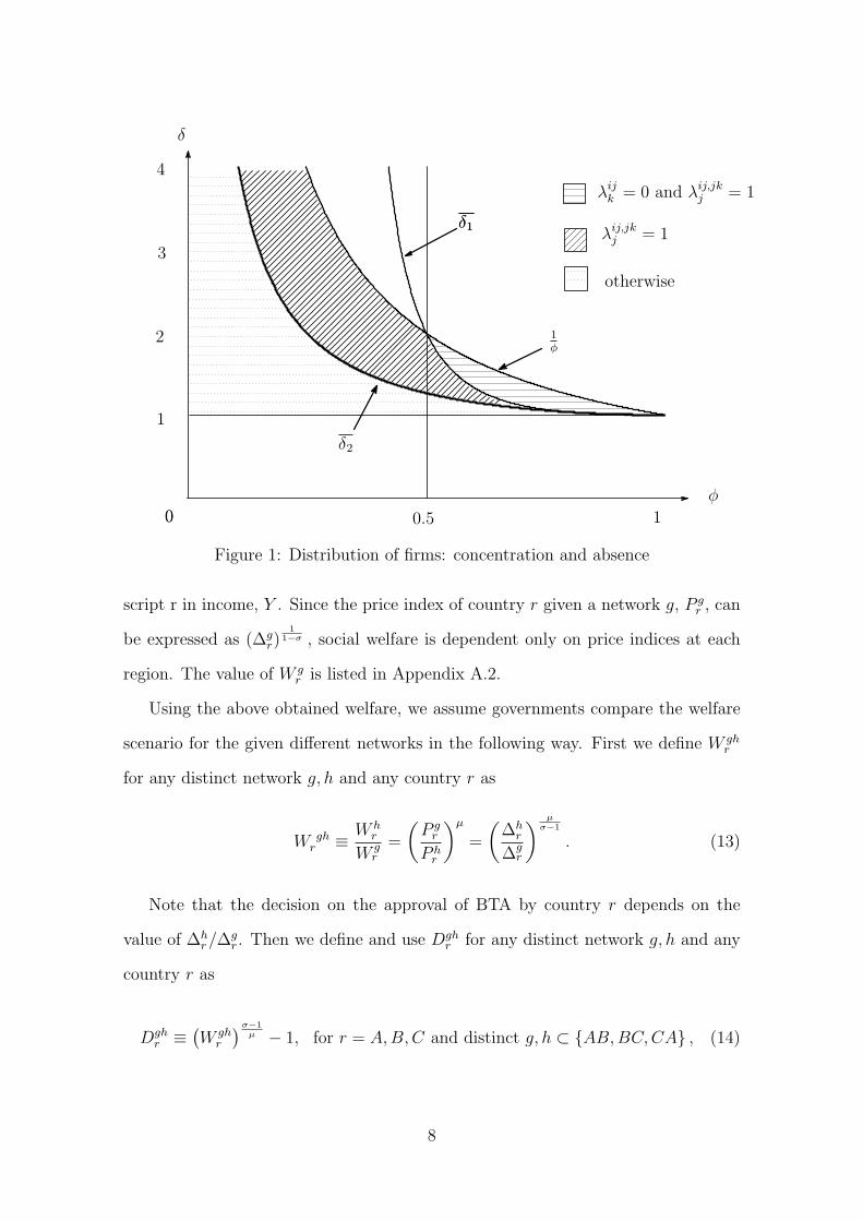
as is listed in Appendix A.1. As is shown in Figure 1, we have two cases of corner

solutions —– the case of λijk = 0 and the case of λ

ij,jkj = 1 for distinct countries

i, j and k. The former one occurs when a given network is ij, where the two coun-

tries i and j share all the firms evenly, and the latter occurs when a given network

ij, jk or what is alternatively called star network, where the hub country j gets

all the firms.

Moreover, we define the objective function of the government, social welfare, of

each country r as the indirect utility function of all residents in the country and it

may be written as

W gr =

Yr

(P gr )µ = Y (∆g

r)µ

σ−1 (12)

Considering the symmetry assumption among the three countries given a particular

population, since wage and capital rent are equal among the countries, the national

(regional) incomes are identical. Thus, without loss of generality, we drop the sub-

7

0φ

δ

0 10.5

1

2

3

4

δ1

1φ

δ2

δ1

λijk = 0 and λij,jk

j = 1

λij,jkj = 1

otherwise

Figure 1: Distribution of firms: concentration and absence

script r in income, Y . Since the price index of country r given a network g, P gr , can

be expressed as (∆gr)

11−σ , social welfare is dependent only on price indices at each

region. The value of W gr is listed in Appendix A.2.

Using the above obtained welfare, we assume governments compare the welfare

scenario for the given different networks in the following way. First we define W ghr

for any distinct network g, h and any country r as

W ghr ≡ W h

r

W gr

=

(P g

r

P hr

)µ

=

(∆h

r

∆gr

) µσ−1

. (13)

Note that the decision on the approval of BTA by country r depends on the

value of ∆hr/∆

gr . Then we define and use Dgh

r for any distinct network g, h and any

country r as

Dghr ≡ (

W ghr

)σ−1µ − 1, for r = A,B, C and distinct g, h ⊂ AB,BC, CA , (14)

8

which implies the welfare change of country r from network g to network h. Fur-

thermore, for the brief notation, we define

Dg+ijr ≡ Dgg∪ij

r (15)

for any network g and any link ij /∈ g. Each government can evaluate their decision

based on this welfare differential in (13). The outcome networks and the corner

solutions where there are no firms in a country or where all firms concentrate in a

single country are summarized in Figure 1. Since profit of monopolistic companies

are constant among any network g, as is shown in Appendix A, the source of trade

agreements the reduction in trade costs resulted from the conclusion of BTA affects

real wage only through price indices, and the distribution of firms.

3 Vision of government

Now, we introduce a simple dynamic game for conclusion-network formation

by national government. Suppose that countries A, B and C are facing situations

to determine which BTA to conclude. Every country is concerned only with its

own social welfare. In order to maximize its own social welfare, each government

organizes conferences to discuss the reduction of trade barriers by BTA. In this

game, we focus only on bilateral conferences and later discuss multilateral conference

case. Each conference has to conclude at most one BTA between participants.

We assume decisions are irreversible so that all countries decide their own actions

without considering the break of connected links.

For further understanding, we specify a word, “Conference”. “Conference” is

defined as a meeting to consult about forming a link between two participating

governments, which represent the end points of the link. The conference on forming

link X is denoted by Conference X for X = AB, BC, CA. In order to clarify the

difference of these networks from the outcome network, we refer to a network formed

9

on the way as “en route network”. In addition, we suppose that the welfare of each

country is not transferable. Hereon, we consider and compare two types ofvision of

governments: myopic and farsighted.

3.1 Myopic games

First, we consider the case that all governments of countries are myopic decision

makers: we suppose that participants of each conference take into account only how

their payoffs change when they link, not how those finally change after all confer-

ences. We denote the conclusion-network formation game with myopic governments

by ΓM (φ, δ). In our paper, we simply call ΓM (φ, δ) the “myopic game” for (φ, δ).

By the above setup, we can assert the result of every conference with each change

of the participant’s social welfare by forming a link: a conference makes a conclusion

to link only if both the welfares of the participants are strictly improved; otherwise

it decides not to link. Moreover, any conference does not make a conclusion once

the previous one determines not to link since it faces the same situation as the

previous one by symmetry. Hence the possible outcome networks are only ∅, AB,AB,BC and AB, BC, CA. Then we show that actually ∅ and AB,BC can

not be outcome networks and exhibit the condition where the outcome network is

complete and where it becomes AB.

Proposition 1 Suppose all the governments of countries make choices myopically,

then the outcome network is always complete.

Therefore, star networks can not be formed due to the fact that there is al-

ways Pareto improvement for region C and A from the conclusion of CA under

AB,BC.

10

3.2 Farsighted games

Next, we consider the case that all governments are farsighted decision makers:

we suppose that they take into account the social welfares gains after all conferences.

Therefore, they make actions thinking over how their actions affect the subsequent

conferences, so that we need to specify the optimal strategy for each country by back-

ward induction. We denote the conclusion-network formation game with farsighted

governments by ΓF (φ, δ). In our paper, we simply call ΓF (φ, δ) the “farsighted

game” for (φ, δ).

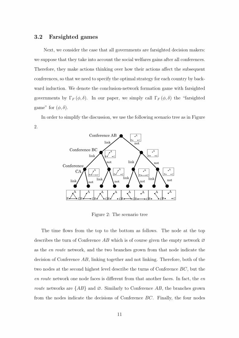
In order to simplify the discussion, we use the following scenario tree as in Figure

2.

Figure 2: The scenario tree

The time flows from the top to the bottom as follows. The node at the top

describes the turn of Conference AB which is of course given the empty network ∅

as the en route network, and the two branches grown from that node indicate the

decision of Conference AB, linking together and not linking. Therefore, both of the

two nodes at the second highest level describe the turns of Conference BC, but the

en route network one node faces is different from that another faces. In fact, the en

route networks are AB and ∅. Similarly to Conference AB, the branches grown

from the nodes indicate the decisions of Conference BC. Finally, the four nodes

11

at the lower level describe the turns of Conference CA, whose en route networks

are respectively AB, BC, AB,BC and ∅, and the eight nodes at the bottom

describe the outcome networks.

With the scenario tree, we analyze the outcomes of the dynamic games compar-

ing it with those of the myopic games. Since we proved that the outcome network

in a myopic game can be the complete network AB, BC,CA , we consider all

the farsighted profiles (φ, δ) at once. When the outcome network is complete in

ΓM (φ, δ), by symmetry, each conference must conclude to link whichever en route

network it faces in ΓF (φ, δ). Hence, the outcome network in ΓF (φ, δ) is also com-

plete. This is the case that strategically avoiding from ending as a star network by

the others, any of two governments agree to conclude BTA for any given en route

network. Summarizing the above, we conclude by the following proposition.

Proposition 2 The outcome of the farsighted game ΓF (φ, δ) is also the complete

network.

4 Discussion and Conclusion

In the process of growing trade networks, we examine pairwise improvements

of trade costs among three countries via bilateral trade agreements. We extensively

analyze the different outcome networks depending on government vision. In the

previous section, we show that myopic and farsighted games never induce a star

network and that for any (φ, δ), the myopic game and farsighted game yields the

complete network. Our results suggest an optimistic view to Krugman’s discussion

that free trade among varioous countries in the world will be achieved regardless of

the vision of governments, even though the world is divided into three symmetric

FTA-regions which gives the worst social welfare.

12

References

Ago, Takanori, Ikumo Isono, and Takatoshi Tabuchi (2006) “Locational disadvan-

tage of the hub,” The Annals of Regional Science, Vol. 40, No. 4, pp. 819–848.

Behrens, Kristian (2007) “On the location and lock-in of cities: Geography vs trans-

portation technology,” Regional Science and Urban Economics, Vol. 37, No.

1, pp. 22–45.

Behrens, Kristian, Carl Gaigne, Gianmarco I.P. Ottaviano, and Jacques-Francois

Thisse (2006) “Is remoteness a locational disadvantage?” Journal of Economic

Geography, Vol. 6, No. 3, pp. 347–368.

Bhagwati, Jagdish and Arvind Panagariya (1996) “Preferential Trading Areas and

Multilateralism: Strangers, Friends or Foes?” in Jagdish Bhagwati and Arvind

Panagariya eds. The Economics of Preferential Trading Agreements, Washing-

ton, D.C.: AEI Press, pp. 1–78.

Furusawa, Taiji and Hideo Konishi (2007) “Free trade networks,” Journal of Inter-

national Economics, Vol. 72, No. 2, pp. 310–335.

Krugman, Paul (1993a) “The Hub Effect: Or, Threeness in International Trade,”

in J. Peter Neary ed. Theory Policy and Dynamics in International Trade:

Essays in Honor of Ronald Jones, Cambridge: Cambridge University Press.

(1993b) “Regionalism Versus Multilateralism: Analytical Notes,” in Jaime

de Meolo and Arvind Panagarya eds. New Dimensions in Regional Integration,

Cambridge: Cambridge University Press.

Mori, Tomoya and Koji Nishikimi (2002) “Economies of transport density and in-

dustrial agglomeration,” Regional Science and Urban Economics, Vol. 32, No.

2, pp. 167–200.

13

Mukunoki, Hiroshi and Kentaro Tachi (2006) “Multilateralism and Hub-and-Spoke

Bilateralism,” Review of International Economics, Vol. 14, No. 4, pp. 658–674.

Appendix A

A.1 Distribution of firms

By specifying each phase, we explicitly solve for the distribution of firms and

the welfare differential for each countries. While the rotation of the conferences are

specified in this appendix, due to the symmetry of three countries the results remain

unchanged.

A.1.1 Profit at each phase

From the assumption of equally endowed capital and normalization in wage, popu-

lation and the number of firms, the reward from capital can be written as Nπ/3 =

π/3 (= k) . Plugging this capital reward into the regional income in (2) with (11),

then we may rewrite equation (11) as πg = Y Ωg =(1 + πg

3

)Ωg where Ωg ≡

µ/σ∑

r=A,B,C φgsr/∆

gs expresses the distribution of firms weighted by distance. Solv-

ing for the profit at any phase, we have, πg = Ωg

1−Ωg/3. From the capital arbitrage

results which follows below, the equilibrium at each phase Ω is the same regardless

of location. Moreover, substituting the above mentioned variables into (11), obtain-

ing the result, Ωg = 3µ/σ, ∀g is straightforward. Thus profit is constant across all

networks.

A.1.2 Empty network and complete networks

The solution for the distribution of firms are given by

λgA = λg

B = λgC = 1

3, where g = φ or AB, BC,CA

14

A.1.3 When the network has only one link

Let i, j and k be distinct countries. Suppose that a BTA is concluded only

between countries i and j. Applying the capital arbitrage condition, the solution

for the distribution of firms are given by

λiji = λ

ijj = 1

3−3φ+φ2+δφ+1

(1−φ)(−2φ+δφ+1)> λ

ijk

λijk = 1

3

φδ(1−3φ)+(4φ2−3φ+1)(1−φ)(−2φ+δφ+1)

Note that although λgr should not exceed 1 and zero, keeping the restriction of

δφ < 0, we have λgr ∈ [0, 1]. We have the case such that λ

ijk = 0 and λ

iji =

λijj = 1

2. Equating to zero, we have the critical value for this corner solution,

1+4φ2−3φφ(3φ−1)

≡ δ1 ≤ δ < 1φ. When δ exceeds δ1, λ

ijk is always zero. This result is

illustrated in Figure 1.

A.1.4 When the network is a star network with two links

Suppose that BTAs are concluded between countries i and j and between coun-

tries j and k. Let i, j and k distinct.

As is the same procedure for A.1.2, we obtain the solution for the distribution

of firms by,

λij.jki = λ

ij.jkk = 1

3φ+δ2φ2−3δφ+1

(1−δφ)(1−φ(2δ−1))< λ

ij.jkj

λij.jkj = 1

3φ+4δ2φ2−3δφ−3δφ2+1

(δφ−1)(−φ+2δφ−1)

Restriction in the parameter, δφ < 0, allows us to keep the variable of interest in

the reasonable range, λgr ∈ [0, 1]. We have the case such that λ

ij.jki = λ

ij.jkk = 0

and λij.jkj = 1. The critical value for this corner solution is 3−√

5−4φ2φ

≡ δ2 ≤ δ < 1φ.

When δ exceeds δ2 in the possible range, λij.jki and λ

ij.jkk are always zero. This

result is illustrated in Figure 1.

15

A.2 Welfare

Using the above results, (12) and (13), we obtain welfare and decision criteria for

each country at each phase as in Table 1 and 2. The conditions listed in the table

indicate that λijk = 0 when δ1 ≤ δ < 1

φand λ

ij,jkj = 1 when δ2 ≤ δ < 1

φ, which is

obtained in Appendix A.1.

W φr W

ijr W

ij,jkr W

ij,jk,kir

r = i 1+2φ3

1+δφ2

when λijk = 0

δφ+1−2φ2

3(1−φ)otherwise

δφ when λij,jkj = 1

1+φ−2δ2φ2

3(1−δφ)otherwise

1+2δφ3

r = j 1+2φ3

1+δφ2

when λijk = 0

δφ+1−2φ2

3(1−φ)otherwise

1 when λij,jkj = 1

2δ2φ2−1−φ3(2δφ−1−φ)

otherwise1+2δφ

3

r = k 1+2φ3

φ when λijk = 0

δφ+1−2φ2

3(δφ+1−2φ)otherwise

δφ when λij,jkj = 1

1+φ−2δ2φ2

3(1−δφ)otherwise

1+2δφ3

Table 1: Welfare of three countries

16

Dφ+

ijr

Di

j+

jkr

Di

j,jk

+ki

rD

13

r

r=

i3δφ+

1−4

φ2(2

φ+

1)

>0

when

λ1 C

=0

(δ−1

)φ(2

φ+

1)(

1−φ

)>

0ot

her

wis

e

−1−δ

φ1+

δφ

<0

when

λ1 C

=0

and

λ2 B

=1

2φ

2−3

δφ

2+

2δφ−1

δφ+

1−2

φ2

<0

when

λ2 B

=1

2φ−δ

2φ

2−1

3(1−δ

φ)(

δφ+

1)<

0w

hen

λ1 C

=0

−φ

2(δ−1

)(δ(1−φ

)+1−δ

φ)

(1−δ

φ) (

δφ+

1−2

φ2)

<0

other

wis

e

1 31−δ

φδφ

>0

when

λ1 C

=0

and

λ2 B

=1

1 31−δ

φδφ

>0

when

λ2 B

=1

(δ−1

)φ

φ−2

δ2φ

2+

1>

0w

hen

λ1 C

=0

(δ−1

)φ

φ−2

δ2φ

2+

1>

0ot

her

wis

e

−1−δ

φ3(1

+δφ)<

0w

hen

λ1 C

=0

2φ(1 2

−φ)(

δ−1

)

1+

δφ−2

φ2

other

wis

e

r=

j3δφ+

1−4

φ2(2

φ+

1)

>0

when

λ1 C

=0

(δ−1

)φ(2

φ+

1)(

1−φ

)>

0ot

her

wis

e

1−δ

φ1+

δφ

>0

when

λ1 C

=0

and

λ2 B

=1

3φ−2

φ2+

δφ−2

2φ

2−δ

φ−1

>0

when

λ2 B

=1

−1 3−φ

+2δ2φ

2+

3δφ−3

δφ

2−1

(−φ+

2δφ−1

)(δφ+

1)

>0

when

λ1 C

=0

φ(δ

−1)

φ+

2φ

2−2

δφ

2−1

(−φ+

2δφ−1

) (−2

φ2+

δφ+

1)

>0

other

wis

e

−2(1−δ

φ)

3<

0w

hen

λ1 C

=0

and

λ2 B

=1

−2(1−δ

φ)

3<

0w

hen

λ2 B

=1

2δφ

2(δ−1

)

−φ+

2δ2φ

2−1

<0

when

λ1 C

=0

2δφ

2(δ−1

)

−φ+

2δ2φ

2−1

<0

other

wis

e

−1−δ

φ3(1

+δφ)<

0w

hen

λ1 C

=0

2φ(1 2

−φ)(

δ−1

)

1+

δφ−2

φ2

other

wis

e

r=

k−

1−φ

2φ+

1<

0w

hen

λ1 C

=0

−2φ

2(δ−1

)(2

φ+

1)(−2

φ+

δφ+

1)<

0ot

her

wis

e

δ−

1>

0w

hen

λ1 C

=0

and

λ2 B

=1

2φ

2+

3δ2φ

2+

2δφ−6

δφ

2−1

−2φ

2+

δφ+

1>

0w

hen

λ2 B

=1

1 32φ+

2δ2φ

2−3

δφ

2−1

φ(δ

φ−1

)>

0w

hen

λ1 C

=0

φ(δ

−1)

2δ2φ

2+

δφ−2

δφ

2−1

(δφ−1

) (−2

φ2+

δφ+

1)

>0

other

wis

e

1 31−δ

φδφ

>0

when

λ1 C

=0

and

λ2 B

=1

1 31−δ

φδφ

>0

when

λ2 B

=1

(δ−1

)φ

φ−2

δ2φ

2+

1>

0w

hen

λ1 C

=0

(δ−1

)φ

φ−2

δ2φ

2+

1>

0ot

her

wis

e

δ−

1+

1−δ

φ3φ

>0

when

λ1 C

=0

2φ(δ−1

)(1−φ

+δφ)

1+

δφ−2

φ2

>0

other

wis

e

Tab

le2:

Dec

isio

ncr

iter

iafo

rB

TA

17

Appendix B

B.1 The proof of Proposition 1

Proof. We check the condition to form a link at each conference:

Conference AB Dφ+ABA > 0 and Dφ+AB

B > 0, so δ > 1. Therefore countries A and

B always link together.

Conference BC By the result of Conference AB, the en route network Conference

BC faces is AB. In any case, DAB+BCB > 0 and D

AB+BCC > 0 always

hold. Therefore countries B and C always link together.

Conference CA By the result of Conference AB and Conference CA, the en route

network Conference CA faces is AB,BC. In any case, DAB,BC+CAC > 0

and DAB,BC+CAA > 0 always hold. Therefore countries C and A always link

together.

Finally, the outcome network of ΓM (φ, δ) is always complete.

B.2 The proof of Proposition 2

Proof. We solve by backward induction. Note that for any distinct i, j and k,

Dφ+iji > 0, D

jk+iji > 0, D

jk+ijj > 0 and D

ij,jk+kii > 0.

Conference CA In any case, Dφ+CAC > 0 and Dφ+CA

A > 0, DAB+CAC > 0 and

DAB+CAA , D

BC+CAC > 0 and D

BC+CAA > 0 and, D

AB,BC+CAC > 0 and

DAB,BC+CAA > 0. Therefore for any en route network, countries C and A

always link together.

Conference BC Conference BC consider the strategy of Conference CA. When the

en route network Conference BC faces is φ, the outcome network is BC, CAif countries B and C conclude a BTA, and CA if not. Since D

CABC,CAB =

18

DCA+BCB > 0 and D

CABC,CAC = D

CA+BCC > 0 in any case, countries B

and C decide to link together. When the en route network Conference BC faces

is AB, the outcome network is AB, BC,CA if countries B and C conclude

a BTA, and AB, CA if not. Since DAB,CAAB,BC,CAB = D

AB,CA+BCB > 0

and DAB,CAAB,BC,CAC = D

CA+BCC > 0 in any case, countries B and C

decide to link together.

Conference AB Conference AB consider the strategies of Conference CA and

Conference BC. Since the en route network Conference AB faces is φ, the

outcome network is AB,BC, CA if countries A and B conclude a BTA,

and BC,CA if not. Since DBC,CAAB,BC,CAA = D

BC,CA+ABA > 0 and

DBC,CAAB,BC,CAB = D

BC,CA+ABB > 0 hold in any case, countries A and B

decide to link together.

Finally, the outcome network of ΓF (φ, δ) is also always complete.

19