Music Information Retrieval Engenharia Informática e de ...

Music Information Retrieval

Developing Tools for Musical Content Segmentation and Comparison

Ricardo Jorge Sebastião dos Santos

Dissertação para obtenção do Grau de Mestre em

Engenharia Informática e de Computadores

Júri

Presidente:

Orientador:

Co-Orientador:

Vogal:

Prof. António Manuel Ferreira Rito da Silva

Prof. David Manuel Martins de Matos

Profª Isabel Maria Martins Trancoso

Prof. António Joaquim dos Santos Romão Serralheiro

Outubro 2010

Acknowledgements

I would like to express my gratitude to Miguel Miranda, who implemented the cutting search algorithm

used in the early attempts to tackle music structure (Section 2.2.2).

My gratitude also goes to Isabel Trancoso, who introduced me to speech processing, to Antonio

Serralheiro for the accurate observations and analysis of this work, and to David Matos for his end-

less enthusiasm, inspiration and guidance.

Above all, I owe the completion of this thesis to my family, from whom I had unconditional support,

and to my companion Sofia, for the continuous motivation.

ii

Resumo

A extracao de informacao em musica e uma disciplina recente que inclui ja multiplas tecnicas sufi-

cientemente maduras para a sua utilizacao no contexto de um conjunto de ferramentas que permita

a automacao de tarefas recorrentes desta disciplina. O objectivo deste trabalho foi a implementacao

de ferramentas em C++ para deteccao de fronteiras de segmentos de musica e repeticoes destes,

assim como para o calculo de medidas de distancia em musica, coerentes com a percepcao humana

de semelhanca entre pecas musicais. Uma consequencia disto foi a criacao de uma consideravel

base de codigo, que pode ser vista como um ponto de partida para futuros melhoramentos e con-

tributos.

Entre as implementacoes mais relevantes, consta a de um filtro de xadrez Gaussiano para a

deteccao de eventos e a de um segmentador com dois estagios de clustering K-Means que detecta

segmentos de uma musica que se repetem. O clustering foi tambem empregue na implementacao

de medidas de distancia entre musicas baseadas na distancia Earth Mover’s (EMD). Varias medidas

de distancia em musica baseadas em clustering foram desenvolvidas, incluindo uma implementacao

da divergencia de Kullback-Liebler para o calculo da distancia entre clusters, assumindo que cada

cluster pode ser aproximado por uma das duas funcoes de densidade de probabilidade implemen-

tadas.

Os resultados obtidos por esta implementacao para a deteccao de eventos em musica, sao

comparaveis aos documentados nos trabalhos usados como referencia, sendo o valor da medida

F obtido de 62%. Os resultados da segmentacao automatica demonstraram que cerca de 71%

dos segmentos identificados como semelhantes tem um valor de distancia efectivamente mais baixo

entre eles. Tambem para as medidas de distancia foram obtidos resultados positivos numa avaliacao

de pequena escala, ainda que mais experimentacao tenha de ser considerada para trabalho futuro.

Keywords

Extracao de Informacao em Musica, Segmentaccao de Musica, Medidas de Distancia em Musica,

Clustering, Divergencia de Kullback-Liebler, Distancia Earth Mover’s.

iii

Abstract

Music Information Retrieval (MIR) is now well established and comprises many techniques that have

matured enough to be used in a context of a toolkit that allows the automation of common tasks in this

discipline. The objective of this work was the implementation of tools in C++ to detect audio segment

borders and repetitions, as well as to determine music distance measures that are consistent with

human perceptions of music. A consequence of this process was the creation of a considerable code

base, which can leverage future improvements and additions.

Among the most relevant, an implementation was made of a Gaussian checker kernel filter for

music on-set detection and a two-stage K-Means clustering-based approach was used to identify

segments that repeat themselves in songs. A clustering-based approach to music distance calcu-

lation, that relies on the Earth Mover’s Distance (EMD), was also implemented. Several distance

measures were developed to compare clusters, including the Kullback-Liebler divergence of cluster

points modelled with one of two different probability density functions that were implemented.

The music on-set detection implementation obtained an F measure of 62% which is comparable to

the results obtained in reference works, and it was shown that the automatic segmentation retrieved

more than 71% of segments determined to be similar by one of the implemented distance measures.

Positive results where obtained for a small scale evaluation of the distance measures developed,

although more extensive experimenting with these tools should be considered in future work.

Keywords

Music Information Retrieval, Music Segmentation, Music Distance Measure, Clustering, Kullback-

Liebler divergence, Earth Mover’s Distance

iv

Contents

Acknowledgements ii

Resumo iii

Abstract iv

List of Figures vii

List of Tables ix

Acronyms and Abbreviations xii

1 Introduction and Objectives 1

1.1 Segmentation . . . . . . . . . . . . . . . . . . . . . . . . . . . . . . . . . . . . . . . . . 2

1.2 Distance Measure . . . . . . . . . . . . . . . . . . . . . . . . . . . . . . . . . . . . . . 3

1.3 Cross Segmentation and Distance Measure Evaluation . . . . . . . . . . . . . . . . . 3

1.4 Objectives . . . . . . . . . . . . . . . . . . . . . . . . . . . . . . . . . . . . . . . . . . . 4

2 Strategies 5

2.1 Feature Extraction and Parametrization . . . . . . . . . . . . . . . . . . . . . . . . . . 5

2.2 Segmentation . . . . . . . . . . . . . . . . . . . . . . . . . . . . . . . . . . . . . . . . . 7

2.2.1 Border Extraction from Autocorrelation Matrices . . . . . . . . . . . . . . . . . 7

2.2.2 Music Structure Analysis by Finding Repeated Parts . . . . . . . . . . . . . . . 9

2.3 Clustering-Based Segmentation . . . . . . . . . . . . . . . . . . . . . . . . . . . . . . 10

2.3.1 Use of Clustering for L1 Label Extraction . . . . . . . . . . . . . . . . . . . . . 11

2.4 Distance Measures . . . . . . . . . . . . . . . . . . . . . . . . . . . . . . . . . . . . . . 12

2.4.1 EMD as a Song Distance Metric . . . . . . . . . . . . . . . . . . . . . . . . . . 14

2.4.2 Euclidean Distance of Clusters . . . . . . . . . . . . . . . . . . . . . . . . . . . 15

2.4.3 Cluster Covariance Distance Measure . . . . . . . . . . . . . . . . . . . . . . . 15

v

2.4.4 Kullback-Liebler Divergence . . . . . . . . . . . . . . . . . . . . . . . . . . . . . 15

2.4.5 PDFs for Cluster Comparison . . . . . . . . . . . . . . . . . . . . . . . . . . . . 16

3 Architecture 17

3.1 Overview . . . . . . . . . . . . . . . . . . . . . . . . . . . . . . . . . . . . . . . . . . . 17

3.2 Basic Data Structures . . . . . . . . . . . . . . . . . . . . . . . . . . . . . . . . . . . . 17

3.2.1 Use of the C++ Standard Template Library . . . . . . . . . . . . . . . . . . . . 19

3.3 Processing Chains . . . . . . . . . . . . . . . . . . . . . . . . . . . . . . . . . . . . . . 19

3.4 Song Data Modelling and Comparison . . . . . . . . . . . . . . . . . . . . . . . . . . . 22

3.5 External Dependencies and Contributions . . . . . . . . . . . . . . . . . . . . . . . . . 24

4 Evaluation 26

4.1 Corpora . . . . . . . . . . . . . . . . . . . . . . . . . . . . . . . . . . . . . . . . . . . . 27

4.2 Performance Measures . . . . . . . . . . . . . . . . . . . . . . . . . . . . . . . . . . . 28

4.2.1 Matching Tolerance . . . . . . . . . . . . . . . . . . . . . . . . . . . . . . . . . 29

4.2.2 Song Segment Distance Measure . . . . . . . . . . . . . . . . . . . . . . . . . 31

4.2.3 Success Metric for Song Distance . . . . . . . . . . . . . . . . . . . . . . . . . 33

4.3 Gaussian Checker Kernel Filter Border Matching Evaluation . . . . . . . . . . . . . . . 34

4.4 Evaluation of the Cluster Based Automatic Segmentation . . . . . . . . . . . . . . . . 36

4.4.1 Border Matching . . . . . . . . . . . . . . . . . . . . . . . . . . . . . . . . . . . 36

4.4.2 Inter-Segment Distance Evaluation . . . . . . . . . . . . . . . . . . . . . . . . . 37

4.4.3 Empirical Evaluation of the Cluster Based Segmentation Results . . . . . . . . 39

4.5 Evaluation of Distance Measures . . . . . . . . . . . . . . . . . . . . . . . . . . . . . . 41

5 Conclusion 43

5.1 Result Summary and Discussion . . . . . . . . . . . . . . . . . . . . . . . . . . . . . . 43

5.2 Future Work . . . . . . . . . . . . . . . . . . . . . . . . . . . . . . . . . . . . . . . . . . 44

5.3 Objectives versus Challenges . . . . . . . . . . . . . . . . . . . . . . . . . . . . . . . . 45

References 46

Appendix A A1

A Border Matching Results from Gaussian Checker Kernel Matrix and Clustering Based

Segmentation A1

Appendix B B7

vi

B Segment Similarity Results of the KL Divergence of a Single Gaussian per Feature Dis-

tance measure B7

Appendix C C11

C Small Scale Evaluation of Song Distance Measure Results C11

vii

List of Figures

2.1 Example distance matrix obtained from the song “Thank you” by Alannis Morriset . . . 8

2.2 Gaussian checker filter matrix representation with a side of 40 and a standard deviation

of 24 . . . . . . . . . . . . . . . . . . . . . . . . . . . . . . . . . . . . . . . . . . . . . . 9

2.3 Sequence of low level labels (hmm state assignements) per beat against a manual

segmentation . . . . . . . . . . . . . . . . . . . . . . . . . . . . . . . . . . . . . . . . . 11

2.4 Manual annotations and low level labels from the filtered cluster assignment of each

musical frame . . . . . . . . . . . . . . . . . . . . . . . . . . . . . . . . . . . . . . . . . 11

2.5 Overview of the cluster based segmentation process . . . . . . . . . . . . . . . . . . . 12

2.6 Overview of the distance measure process flow . . . . . . . . . . . . . . . . . . . . . . 13

3.1 Overview of the tool chain used to produce results with Shkr. . . . . . . . . . . . . . . 18

3.2 Gaussian checker kernel processing chain UML class diagram . . . . . . . . . . . . . 20

3.3 Code listing of the Gaussian checker kernel segmentation chain . . . . . . . . . . . . 21

3.4 Cluster-based segmentation chain UML class diagram . . . . . . . . . . . . . . . . . . 22

3.5 Code listing for the creation of the clustering based segmentation chain . . . . . . . . 23

3.6 Overview of the song and cluster data modelling . . . . . . . . . . . . . . . . . . . . . 25

4.1 Example of an ambiguous border location between a verse and a bridge . . . . . . . . 30

4.2 Precision, recall and F measure of the Gaussian checker kernel filter . . . . . . . . . . 35

4.3 Border matching performance measures for cluster based approach . . . . . . . . . . 37

4.4 Self-similarity distance evaluation results for the automatic segmentations . . . . . . . 38

4.5 Average total labels and correct labels from GT and AS for the range of tested L2

clusters. . . . . . . . . . . . . . . . . . . . . . . . . . . . . . . . . . . . . . . . . . . . . 39

4.6 Segmentation view for “Wonder Wall” from Oasis, with the 3 L2 clusters . . . . . . . . 40



4.9 Segmentation view for “Wonder Wall” from Oasis, from ground truth annotations . . . 40

viii

4.10 Overview of the tested cluster distance measures versus the number of clusters used. 41

A.1 List songs with corresponding recall and precision, sorted by recall for the a Gaussian

matrix side of 20 and a Gaussian standard deviation of 12 . . . . . . . . . . . . . . . . A3





A.4 List songs with corresponding recall and precision, sorted by recall for the clustering

based segmentation using 5 clusters L2 and 80 clusters L1. . . . . . . . . . . . . . . . A6

C.1 Comparison of the tested cluster distance measures using 1 cluster. . . . . . . . . . . C12

C.2 Comparison of the tested cluster distance measures using 10 clusters. . . . . . . . . . C13

C.3 Comparison of the tested cluster distance measures using 20 clusters. . . . . . . . . . C14

ix

List of Tables

2.1 List of features used by several authors in related work with the corresponding tasks

in for which they were used. . . . . . . . . . . . . . . . . . . . . . . . . . . . . . . . . . 6

2.2 Parametrization of the MFCC extraction. . . . . . . . . . . . . . . . . . . . . . . . . . . 7

4.1 Example of self segment similarity comparison for the ground truth segments . . . . . 31

4.2 Example of self segment similarity per label average distances for the ground truth

segments . . . . . . . . . . . . . . . . . . . . . . . . . . . . . . . . . . . . . . . . . . . 32

4.3 Border matching performance measures of the Gaussian checker kernel filter . . . . . 34

4.4 Border matching performance measures for cluster based approach . . . . . . . . . . 36

4.5 Self-similarity distance evaluation results for the automatic segmentations . . . . . . . 38

4.6 Overview of the tested cluster distance measures versus the number of clusters used 41

A.1 Detailed border matching performance measures of the Gaussian checker kernel filter A1

A.2 Border matching performance measures for cluster based approach for the range of

tested L2 cluster values . . . . . . . . . . . . . . . . . . . . . . . . . . . . . . . . . . . A2

B.1 Segment self-similarity matrices used to validate empirically the KL divergence of the

single Gaussian per features distance measure . . . . . . . . . . . . . . . . . . . . . . B8

B.2 Self-similarity distance evaluation results for the segmentations obtained with the range

of tested L2 cluster values . . . . . . . . . . . . . . . . . . . . . . . . . . . . . . . . . . B9

B.3 Segment self-similarity results for all songs in the corpus, for an automatic segmenta-

tion using 5 L2 clusters . . . . . . . . . . . . . . . . . . . . . . . . . . . . . . . . . . . B10

C.1 List of songs which compose the small scale evaluation corpus of distance measures. C11

C.2 Results of the different cluster distance measures for all of the corpus categories with

only 1 cluster in comparison . . . . . . . . . . . . . . . . . . . . . . . . . . . . . . . . C12


10 clusters clusters in comparison . . . . . . . . . . . . . . . . . . . . . . . . . . . . . C12

x


20 clusters clusters in comparison . . . . . . . . . . . . . . . . . . . . . . . . . . . . . C13

xi

Acronyms and Abbreviations

AS Automatic SegmentationBPM Beats Per MinuteCQT Constant Q TransformCRS Content Recommendation SystemDOM Document Object ModelDTW Dynamic Time WarpingEMD Earth Mover’s DistanceGT Ground TruthHMM Hidden Markov ModelHPCP Harmonic Pitch Class ProfileISMIR International Society for Music Information RetrievalKL-divergence Kullback-Liebler divergenceL1 Level 1 (clusters)L2 Level 2 (clusters)LPC Linear Prediction CoefficientsMFCC Mel Frequency Cepstral CoefficientsMILP Mixed Integer Linear ProgrammingMIR Music Information RetrievalMIREX Music Information Retrieval Evaluation eXchangeMP3 MPEG Layer 3MPEG Moving Picture Experts GroupPCA Principal Component AnalysisPDF Probability Density FunctionPNM Portable Anymap FormatShkr ShakiraSTFT Short Time Fourier TransformSTL Standard Template LibrarySVM Support Vector Machines

xii

Chapter 1

Introduction and Objectives

Music in digital format is now widely spread, this being the consequence of more than two decades

passed over the audio CD introduction. Advances in audio encoding systems (e.g. MPEG layer 3), as

well as the widespread of high-capacity storage devices, allowed for the creation of the digital music

library concept. The high availability and demand for such content created new requirements about

its management, distribution and advertisement, that suggest a more direct analysis of the content

than that provided by simple human driven meta-data cataloguing of the music.

In addition, this large volume of information, combined with the processing power to analyse it,

allows for the posing of long standing questions, that formerly were only approachable by music

theoretical analysis, such as correlating ethnic music with the cultures where it spawns as mentioned

by Howes [1]:

There is thus a vast corpus of music material available for comparative study. It would be

fascinating to discover and work out a correlation between music and social phenomena

Frank Howes, 1948

In light of the new technological advances and possibilities, a new discipline of Information Re-

trieval gained traction, Music Information Retrieval (MIR), which uses music as its dataset. The

development of new computational methods and tools for pattern finding and comparison of musi-

cal content is currently a very active research area where different methods and applications are

constantly being developed. An example of this is the annual Music Information Retrieval Evaluation

eXchange (MIREX) [2] contest that is coupled to the International Society (and Conference) for Music

Information Retrieval (ISMIR) [3]. Evaluated tasks include Automatic Genre Identification, Query by

Humming, Chord Detection, Segmentation, Melody Extraction, to name a few.

This work describes a preliminary effort to develop a toolkit written in C++ for common tasks

in music retrieval, aiming at the integration of a music Content Recommendation System (CRS),

1

covering two common tasks in this field that have a broad range of applications. These are music

segmentation into humanly identifiable musical segments, and music similarity measures. Over the

next chapters, it will be referred to as the Shkr project.

Over the next sections of this chapter, the objectives and applications of the work developed in the

segmentation and similarity measures are presented. The strategies used for music segmentation

and similarity are developed in chapter 2, followed by a description of the implemented architecture in

chapter 3. The methods of evaluation and results for each solution are described in chapter 4. Notes

for future work, conclusions and general result discussion considerations are included in chapter 5.

1.1 Segmentation

Finding the boundaries of sections - time-spans - of audio that are different from each other is a

commonly used strategy to determine an underlying structure in music content. Since music can

be seen - and written - as a sequence of events, reliably determining the boundaries and duration

of such events is a prerequisite in many MIR-related tasks. Example musical events can be notes,

chords, groups of notes or chords, volume (signal energy) alterations, timbre alterations (e.g. different

instruments present, different octaves played), rhythm changes, singing to non-singing transitions, to

mention a few of the most relevant.

Segmentation is a direct consequence of musical composition and production. An example is

the interval between a dominant beat in a modern Pop song, usually characterised by the timespan

between a high energy, low frequency pulse, created by a percussion or bass instrument, which

is a property commonly used for sound loop extraction and processing in musical remixes. On a

different scale, a musical score can also be seen as a formalization of a desirable sequence of

events, with different durations and acoustic characteristics, during which, or in the interval of which,

a segmentation can emerge, e.g. predominant scales, key and other aspects of musical harmony.

The difference between these two examples of segmentation is therefore the granularity (scale) and

nature (features) of the events that define a musical segment.

In this work, focus was given to detecting the humanly perceivable portions of popular music

that are commonly mentioned as “choruses”, “verses”, “intros”, “bridges” or “breaks” and are usually

repeated (sometimes with variations). This specific segmentation task was approached by several

researchers (as further developed in Chapter 2 ), although the range of musical genres to which it is

applicable is reduced, since it does not typically occur in all of them. Only Pop and Rock music was

used in the segmentation evaluation corpus, in order to limit the scope of the evaluation to genres

where this type of segmentation is usually applicable.

2

Target applications of this type of segmentation are typically:

• “Jump to the next section” features in media players, which can allow a first time listener to

quickly browse a song by listening only to the portions of it that are significantly different.

• “Audio thumbnailing”, where segmentation can provide a list of candidate audio excerpts that

can be presented to a listener for fast musical identification or evaluation.

1.2 Distance Measure

Comparing and cataloguing musical content is a complex task that is usually the domain of a human

listener and, more recently, of meta-data driven CRS. In the scope of this work, music distance was

approached as a tool to produce a measure by which an ordered playlist of similar songs in a corpus

can be determined.

Typical applications of such a tools are:

• Suggestion of similar music to a listener, based on the musical signal instead of meta-data tags.

• Playlist generation/sorting (e.g. emphSchnitzer [4])

• Query by Humming (e.g. Midomi [5]).

• Identification of candidate segments for audio “thumbnailing” by cross-comparing audio seg-

ments.

In what concerns music distance measure, the tools produced by this work use documented

methods for comparing audio musical content. However gaps were left in what concerns feature

selection and evaluation, which although pertinent in the scope of the task at hand, would significantly

increase its complexity.

1.3 Cross Segmentation and Distance Measure Evaluation

Segmentation and distance measure can overlap in their evaluation, if the segments obtained from

a song repeat themselves in a musical piece. An assumption was made in the evaluation of the

tools produced, that the application of the distance measure to musical segments that are humanly

annotated as being similar should result in smaller distance values in relation to those that are not.

While human segmentation annotations are not always accurate, it was found that this is generally

the case for the proposed methods.

3

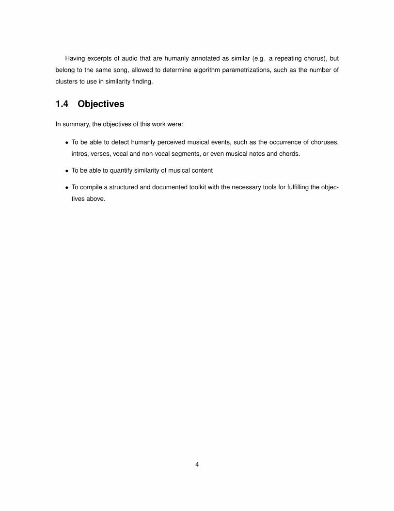
Having excerpts of audio that are humanly annotated as similar (e.g. a repeating chorus), but

belong to the same song, allowed to determine algorithm parametrizations, such as the number of

clusters to use in similarity finding.

1.4 Objectives

In summary, the objectives of this work were:

• To be able to detect humanly perceived musical events, such as the occurrence of choruses,

intros, verses, vocal and non-vocal segments, or even musical notes and chords.

• To be able to quantify similarity of musical content

• To compile a structured and documented toolkit with the necessary tools for fulfilling the objec-

tives above.

4

Chapter 2

Strategies

2.1 Feature Extraction and Parametrization

Features are data elements that characterise particular aspects of the signal. Almost any process

that is a function of the music audio signal and produces related data can be considered a feature

extractor. In MIR, most of the feature extractors are spectrum-centred, meaning that they rely in

short-time Fourier analysis (or other similar transform) to produce frequency domain data. These

methods are usually sensitive to parameters such as the analysis window length and the interval

between analysis windows.

Effort was focussed in the methods and implementations rather that the features being manipu-

lated, since feature selection and parametrization can easily escalate to a combination explosion of

possibilities and this presents challenges that were left outside the scope of this work. Future work

can encompass feature selection towards result optimization.

However, in order to validate the developed methods, it was necessary to employ features that

have been proven to provide results on the previous works in which the implemented solutions are

based on. Table 2.1 presents a compilation of features used by the main authors referenced in this

work.

From the works listed above, it is clear that MFCCs are ubiquitous and hold the potential to

generate good results in several tasks, from segmentation and structure finding to music similarity

measurement. They are expressed in the Mel-Scale, which tries to approximate the human non-

linear perception of pitch, and are processed using short-time analysis of the audio signal. Although

they are known by their applicability in speech recognition, in the context of MIR they are commonly

associated to the discrimination of timbre, which in itself is a combination of several acoustic proper-

ties to which music amply resorts to. An overview of the relations between music and timbre can be

found in the work of Erickson [17].

5

Work Tasks Features Used

Paulus et al. [6] Song segmenta-tion

Chromagram [7] with 36 bins reduced to 15 by PrincipalComponent Analysis (PCA), 13 Mel-Frequency CepstrumCoefficients (MFCCs) [8] including the zeroth coefficient,concatenated with their average and variance.

Levy et al. [9] Music structureidentification

Audio Spectrum Envelope Descriptors of MPEG-7 [10]space with bands space at (1/8)th of an octave.

Logan et al. [11] Music distancemeasure andplaylist generation

12,19 and 29 MFCCs excluding the zeroth coefficient.

Peiszer [12] Music segmenta-tion and structureidentification

40 MFCCs, Constance Q Transform (CQT).

Foote et al. [13] Music structureidentification

Short-Time Fourier Transform (STFT) coefficients andMFCCs.

Ong [14] Music segmen-tation and audio-thumbnailing

36th dimensional Harmonic Pitch Class Profile HPCP (an-other name for Chromagram), MFCCs, Linear PredictionCoefficients (LPC), signal Root Mean Square RMS energyand zero-crossings.

Foote [15] Music segmentboundary finding

STFT coefficients

Ellis et al. [16] Song classificationand artist identifi-cation

20 MFCCs

Schnitzer [4] Automatic genera-tion of playlists ofsimilar music

20 MFCCs obtained from interception of MP3 decoding,before resynthesis to PCM

Table 2.1: List of features used by several authors in related work with the corresponding tasks in for which theywere used.

Given these considerations, MFCCs are good candidate features to use when producing tools

for tasks concerning segmentation and distance measure in music. Therefore MFCCs where the

only feature used in the scope of this work. Although a few experiments were initially made with

Chromagram and LPCs, negative results led the author to use MFCCs to validate the implemented

tools. Table 2.2 contains the MFCC extraction parameters used. For feature extraction, the Hidden

Markov Model Toolkit (HTK) [18] was employed.

A window interval of 100 ms was used since it allows a good frequency domain resolution -

frequencies from 10 Hz are captured and the human hearing lower frequency threshold is around 20

Hz (as mentioned in Huang et al. [19]) - while still providing a time resolution of (1/20)th of a common

song tempo of 120 beats per minute (bpm) which is smaller than the duration of most musical notes

even if the musical piece contains (1/16)th (fast) notes.

Another aspect that may hold a considerable potential for improvement in future work is the use

6

Parameter value

Source Signal Bit Rate 48,000 HzNumber of Channels 1 (stereo colapsed)DC offset subtracted yesNormalization yesWindow Interval 100 msWindow Size 200 msWindow Type HanningNumber of MFCCs 41 - zeroth = 40Cepstrum Lifter Poles 80Pre-Emphasis Coefficient 0.97

Table 2.2: Parametrization of the MFCC extraction.

of automatically identified music temporal measures such as Beat and Meter. Since most feature

extraction processes rely on short-time audio analysis (dividing the audio into frames), meter infor-

mation is commonly used for establishing the analysis window length and step size of this short time

analysis for other feature extractors like in Levy et al. [9] and Paulus et al. [6]. Although beat and

meter techniques are commonly used to enhance the feature extraction process in music, they can

also be regarded as time domain features and be used in the same way as the above listed features,

to increase the available information about the musical content.

2.2 Segmentation

Over this Section, several approaches used for music segmentation are discussed. The term “seg-

ment border” is used when referring to points in a musical piece timeline where musical events and

changes (also referred to as on-sets) occur. “Segments” refer to spans of time in the music that are

encompassed between “borders” and “labels” are tags given to segments which allow the grouping

of similar or repeated “segments”.

2.2.1 Border Extraction from Autocorrelation Matrices

A widely used method to determine the boundaries of “events” in music was introduced by Foote [15].

It is a strategy for finding on-sets in audio where a significant change occurs. In the original work,

Short-Time Fourier Transform coefficients were used as features, although in other works such as

those of Ong [14] and Paulus et al. [6] MFCCs were used to produce the correlation matrices which

this process relies on.

An important step for this method is the calculus of a distance matrix, also referred to as a corre-

lation matrix. The calculus of a distance matrix takes a measure of vector distance, typically either

7

the cosine of the angle between feature vector parameters or the Euclidean distance (used in this

work), and applies it to each feature vector pair extracted, mapping its results in a two dimensional

matrix containing the distances between all vector combinations.

Time Sequence of the Features

Tim

e S

equence

of

the F

eatu

res

Figure 2.1: Example distance matrix obtained from the song “Thank you” by Alannis Morriset. Guide arrowswere included to point the time sequence of the feature vectors that were compared with an Euclidean distance.The transversal black diagonal confirms that the song is equal to itself, since the distance of the features alongthat line is zero, which is mapped to black in the image.

A distance matrix, such as that in Figure 2.1 has a typical checker pattern, and transitions between

checkers that can be mapped to audible musical events. The automatic identification of the visible

8

pattern transitions can be done by calculating the correlation of the distance matrix with a smaller

Gaussian checker kernel matrix, along the distance matrix’s diagonal as described in by Foote [15].

This process produces a vector, the maxima of which correspond to the the pattern transitions seen

on the distance matrix and therefore the musical events borders, though the resolution of the transi-

tions identified varies significantly depending on the system’s parametrization. Figure 2.2 presents

an example of a Gaussian checker with obtained from a Gaussian with a standard deviation of 24.

Figure 2.2: Gaussian checker filter matrix representation with a side of 40 and a standard deviation of 24 - Notethat, in the context of this work, these units should be seen in terms of frames of song audio.

Additionally, a moving average filter with a range of 40 frames is used on the retrieved borders, to

improve the accuracy of the results. The peaks of the resulting vector constitute the resulting set of

borders matched.

2.2.2 Music Structure Analysis by Finding Repeated Parts

In methods that rely on vector space onset detection, such as that presented in Section 2.2.1, where

there is an explicit segment border extraction step, it is not evident which of the identified boundaries

belong to each segment. In the scope of this thesis, we explored the method used by Paulus et al.

9

[6], in which segments are identified from a set of possible segment boundaries1.

This method uses a cutting search improved, brute force comparison of all possible combinations

of identified segment borders (with a method similar to that exposed in Section 2.2.1), and deter-

mines their similirity using a Dynamic Time Warping (DTW) algorithm (which was also implemented).

Each combination of two similar borders is considered a viable segment, and from all possible com-

binations of segments, similar non-overlapping ones are grouped together to form segment groups.

Finally, each combination of non-overlapping segment groups is given a score, and the structural

view of the music emerges from the highest scoring group combination, that is referred to as an

“explanation”.

While this early attempt to produce a viable implementation of a segmentation strategy was not

brought forward due to the challenges posed by finding a useful parametrization of the cutting search

algorithm, the effort invested in it added positive contributions, such as the implementation of the

Group and Segment data structures, still widely used in Shkr for evaluation tasks. Another contribution

was the implementation of DTW.

Dynamic time Warping [19] is a widely used dynamic programming algorithm for comparing audio

signals which might have a slight difference in duration or speed and is widely used in speech recog-

nition for this property. Its complexity is quadratic, but for comparing small segments of audio, this

does not usually pose a problem. It can be considered the first audio distance metric implemented in

the scope of this thesis, although it is not appropriate for the tasks approached by the other distance

measures implemented in this work.

2.3 Clustering-Based Segmentation

The cluster-based segmentation approach used in this work is based on the one proposed by Levy

et al. [9], of which the implementation used in the Segmentation plug-in freely available for Sonic

Vizualizer [21]. In that work, a hidden Markov model (HMM) with 40 states was trained with 21-

dimensional AudioSpectrumProjection [10] feature vectors extracted from the song. The features

are subsequently Viterbi-decoded using the trained model and the sequence of most likely state

assignments is retrieved for each beat of the song. This results in the sequence of “low-level” labels

which in this work will be referred to as L1 - Level 1 - labels (or clusters).

In Levy et al. [9] it is further shown that the “high-level” labels can be extracted by using histograms

of state assignments taken from a sliding window of beats, and then using K-Means clustering, with a

lower number of clusters (as much as the desired number of “high-level” labels), to group the resulting1This was thanks to the contribution of Miguel Miranda [20], who implemented the cutting search algorithm.

10

Figure 2.3: From Levy et al. [9] - Sequence of low level labels (hmm state assignements) per beat, shownagainst the manual annotation segments, which correspond to the regions of different colours. Equal coloursrepresent segments annotated as similar.

Figure 2.4: Manual annotations correspond to the colour regions, where equal colours represent segmentsannotated as similar. Low level labels result from the L1 cluster assignments of a 10 cluster K-Means, althoughthe depicted data points correspond to the mode of the cluster assignments for each 60 frame window (”modefilter”), with which the underlying repeated cluster assignment structures are more apparent. Note that similarsegments have similar cluster assignments for several of the song’s segments.

histograms. The “high-level” labels are referred to as L2 (Level 2) labels or clusters in this work. In

the work of Levy et al., further improvements are suggested to the L2 clustering process, which were

not used, but should be considered for future work.

2.3.1 Use of Clustering for L1 Label Extraction

The relation between Levy et al. and the method used in this work was established when, from

experimentation and prototyping, it was observed that a similar L1 sequence of cluster assignments

could emerge by using K-Means clustering directly on the features extracted from the music signal.

Looking at the cluster assignments of each frame as L1 labels patterns similar to those depicted

in 2.3 were observed as shown in 2.4. The remaining portion of the algorithm is therefore similar

to that of Levy et al.. Note that histograms of L1 cluster assignments obtained from fixed width (in

11

frames) sliding windows, ensure a time continuity of the segments obtained from the L2 clustering.

Good experimental results were determined for 80 L1 clusters and 3 to 10 L2 clusters. Similar to

what was found by Levy et al.. Changing the histogram window size, did not translate in significant

improvements. Figure 2.5 presents a high-level overview of this process.

Figure 2.5: Overview of the cluster-based segmentation process, including the stages of the cluster basedsegmentation.

2.4 Distance Measures

The ability to compute an audio similarity measure is a frequent task in MIR. A simple method for

calculating audio distance measure is DTW, which is documented to have good results when applied

to short audio sequences, as discussed in Section 2.2.2. However, to be able to compare entire

songs, and do so in a way in which playlists can be derived from ranking the distances between

songs suggests the use of a more sophisticated approach.

The concept for distance measure used in this work departed mainly from the work of Logan

et al. [11] and also in a smaller extent by Ellis et al. [16]. In both, classifiers (K-Means clustering

and Support Vector Machines (SVM), respectively) are used to reduce the dimensionality of the input

features and in both Probability Density Functions (PDF) are computed from the the resulting classes,

that can then be compared using measures such as the Kullback-Liebler Divergence [19].

• Ellis et al. [16] describes a technique aimed at artist identification, making use of SVMs for the

task of classifying each song as belonging to a specific artist. A mean vector and a covariance

matrix is determined from a set of 20 MFCC vectors per frame, extracted from each song. The

12

Kullback-Leibler divergence and the Mahalanobis [19] distance were used as distance mea-

sures in the SVM-based classification process. The work concludes that there is an advantage

in the use of SVM classification and the Kullback-Leibler divergence, when compared with other

song classification methods/distance measures.

• Logan et al. [11] song signatures are obtained from the k-means clustering (using 16 clus-

ters) of 12, 19 and 29 dimensional MFCC feature vectors. The Euclidean distance is used as

a distance measure for the clustering process. The signatures are composed of each clus-

ter’s mean, covariance, and weight. The song distance is measured using the EMD distance,

which is used to determine the minimum “work” of transforming one signature into another.

For comparison of a large corpora of music, the signatures for all songs in the corpora are

computed and the distance between signatures is determined. Subjective evaluation was used

for the song similarity with, concluding that for each set of top 5 similar songs retrieved by the

algorithm, 2.5 where considered similar to the original song by the human evaluators.

An high-level overview of the song distance calculation process sequence in Shkr is presented in

Figure 2.6.

Figure 2.6: Overview of the distance measure process flow. The Earth Mover’s distance is calculated for thecluster signatures (which include the cluster points, their standard deviation and centre) obtained from the twosongs A and B. Another distance measure, such as the Kullback-Liebler divergence, is used to compare eachpair combination of song A and song B clusters.

13

2.4.1 EMD as a Song Distance Metric

The Earth Mover’s distance [22] compares the “work” needed to transform a set of clusters P, where

pi ∈ P and pi = {µ, σ, X} is a cluster signature, into a set of clusters Q, with q j ∈ Q and q j = {µ, σ, X}.

The µ cluster signature parameter is the centre (average vector) of the cluster, σ is the standard

deviation of the cluster’s points, and X is the set of cluster points. As mentioned in Rubner et al. [22],

the objective is to find a flow F = [ fi j] that minimizes the work W:

W(P,Q, F) =m∑

i=1

n∑j=1

di j fi j (2.1)

Where di j is a distance value calculated between cluster signatures (using the KL divergence, for

example) pi ∈ P and q j ∈ Q. The total number of clusters in P and Q is represented by m and n,

respectively. The flow fi j, between cluster pi and cluster q j, reflects the cost of moving “probability

mass” from one cluster to another and it is subjected to a set of constraints:

• “Probability mass” can only be moved from a cluster in P to another in Q and not vice-versa.

• The “weight” of each cluster, which is bound to the number of points that belong to it, determines

the maximum amount of “probability mass” that can be taken from it, for clusters in P, or that

can be moved to it, for clusters in Q.

• The maximum quantity of “probability mass” must be moved from P to Q. If the cluster “weights”

are normalized by the number of data points in each song, then the total existing “probability

mass” is always moved (which is the case of the implementation to which this work refers to).

The earth mover’s distance is then obtained by normalizing the “work” with the total flow:

EMD(P,Q) =

∑mi=1∑n

j=1 di j fi j∑mi=1∑n

j=1 fi j(2.2)

Obtaining the maximum flow that is required for the EMD flux calculus is a dynamic programming

problem, that several algorithms can be used to resolve. The solution used was to formulate the

problem as the minimization of Equation 2.1, given a set of constraints for each cluster in P:

wi =

n∑j=1

fi j (2.3)

Where wi is the normalized “weight” of cluster pi. A similar set of constraints apply for each cluster

in Q:

w j =

m∑i=1

fi j (2.4)

14

Where w j is the normalized “weight” of cluster q j.

The resulting equation system can be efficiently solved by means of a linear equation solver, such

as lpsolve [23].

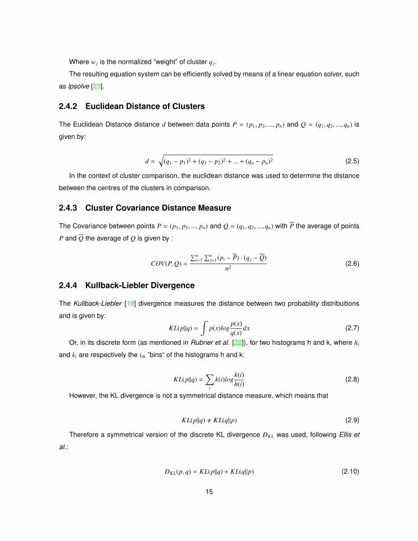
2.4.2 Euclidean Distance of Clusters

The Euclidean Distance distance d between data points P = (p1, p2, ..., pn) and Q = (q1, q2, ..., qn) is

given by:

d =√

(q1 − p1)2 + (q2 − p2)2 + ... + (qn − pn)2 (2.5)

In the context of cluster comparison, the euclidean distance was used to determine the distance

between the centres of the clusters in comparison.

2.4.3 Cluster Covariance Distance Measure

The Covariance between points P = (p1, p2, ..., pn) and Q = (q1, q2, ..., qn) with P the average of points

P and Q the average of Q is given by :

COV(P,Q) =

∑ni=1∑n

j=1(pi − P) · (q j − Q)

n2 (2.6)

2.4.4 Kullback-Liebler Divergence

The Kullback-Liebler [19] divergence measures the distance between two probability distribuitions

and is given by:

KL(p||q) =∫

p(x)logp(x)q(x)

dx (2.7)

Or, in its discrete form (as mentioned in Rubner et al. [22]), for two histograms h and k, where hi

and ki are respectively the ith ”bins“ of the histograms h and k:

KL(p||q) =∑

i

k(i)logk(i)h(i)

(2.8)

However, the KL divergence is not a symmetrical distance measure, which means that

KL(p||q) , KL(q||p) (2.9)

Therefore a symmetrical version of the discrete KL divergence DKL was used, following Ellis et

al.:

DKL(p, q) = KL(p||q) + KL(q||p) (2.10)

15

DKL(p, q) =∑

i

k(i)logk(i)h(i)+∑

i

h(i)logh(i)k(i)

(2.11)

2.4.5 PDFs for Cluster Comparison

Two different PDFs were used in conjunction with the KL divergence - described in Marques [24]. A

Gaussian or Normal Distribution:

p(x) =1√

2πσexp[

(x − µ)2

2σ2 ] (2.12)

Where x is an observation Gaussian distribution, p(x) is the probability of observation µ is the

average of the probability distribution and σ is its variance.

And a Multivariate Gaussian PDF, which was was to model multidimensional clusters features in

a single PDF:

p(x) =1

(2π)n/2|R|1/2exp[−

12

(x − µ)T R−1(x − µ)] (2.13)

Where x is a random variable in �n, µ and R are the average vector and the covariance matrix of

the random variable x.

16

Chapter 3

Architecture

3.1 Overview

Project Shkr is still in a developing stage, and therefore while all of the segmentation and distance

measure algorithms are part of the C++ implemented code base, several external tools are necessary

to provide functionalities such as configuration, audio conversion, and feature extraction. An overview

of these dependencies is presented in Figure 3.1.

From Figure 3.1 it is also visible that there are external dependencies. Audio conversion from

MP3, Ogg [25] or Flac [26] formats is peformed using Sox [27]. The MFCC extractor of the Hidden

Markov Model Toolkit [18] is used to produce the flat files containing the feature values that are used

by Shkr. Future improvements could include moving this part of the processing chain into the Shkr

binary, allowing it to automatically parametrize feature extraction, with information about the music

material analysed, such as beat to determine the size of the audio frame in the short time signal

analysis.

On the output end of the chain song distance measures, segmentation evaluation statistics and

other relevant information to the tasks performed are sent to the standard output of the terminal within

which Shkr must be run. Ground truth annotation is read from a SegmXML format as described in

Peiszer [12] and graphics output can be used to export the contents of a Matrix data structure into

Portable Anymap Format (PNM) of 8bit or 16bit, monochromatic or RGB (Red, Green, Blue) formats.

3.2 Basic Data Structures

The first algorithms and data structures developed in the scope of this thesis were conceived having

in mind simple tasks that were meant to be performed fast, an example being the generation of

correlation matrices from extracted MFCCs listings contained in a flat file. This was a stage where

17

Command line and configuration parsing(init.pl)

C++ Src Code Compilation(makefile/gcc)

SongFeatures

Action Dispatch(mir.sh)

Configuration(common-defs)

User commands

Run Algorithms(shkr binary)

Feature Extraction(Feature_analysis.sh)

Audio Format Conversion(sox)

Feature Extraction(HTK)

Song DistanceResults

WavesurferSegment Borders

and labels

Images andGraphics

Shkr binary

GroundTruth

Annotations

Figure 3.1: Overview of the tool chain used to produce results with Shkr.

the outcomes of the implemented algorithms were more important than their implementation in C++.

An example of this was the creation of the Signal class that encapsulates a vector of FeatureVector

objects which in turn contains an array of features extracted from a song frame, which can also mean

one dimensional sound samples extracted directly from the audio. The Signal data structure is a

dynamically growing structure, particularly useful when new features needed to be added, which

also makes sense in the context of real time audio recording where there is no prior knowledge of

18

the number of samples to store.

Several of the algorithms used were first prototyped in Matlab or Octave, and a considerable

amount of code written for those frameworks is also publicly available from other authors, for example

the MIRtoolbox [28]. In Matlab, matrix manipulation is seamless and therefore algorithm prototyping

for signal processing is fast and clear. From these observations, it was natural that a Matrix data

type, encapsulating a type independent bi-dimensional array of values, was desirable. Therefore the

Matrix class was created and coding matrix manipulation operations was greatly simplified, lever-

aged through the use of C++ operator overloading and templates. The Matrix data type currently

implemented has evolved to allow most of the common matrix calculus operations like matrix multipli-

cation, transposition, sum, among others, and has been partially integrated with Eigen [29] of which

it encapsulates functionality such as matrix inversion and determinant calculus. Yet another useful

matrix operation that it allows, is the creation of sub-matrices via the SubMatrix Class, through the

use of which it is possible to manipulate a smaller sub-set of the values of another matrix as if the

sub-set were also Matrix.

Both Signal and Matrix are elementary building blocks that were used in the implementation of

almost all of the algorithms experimented.

3.2.1 Use of the C++ Standard Template Library

It is noteworthy that almost all of the code base produced in the scope of this work is template driven,

with each class or method requiring at least one template argument. The initial objective of the use

of templates was to make the code type independent, in case it might in future be used in other

platforms like mobile devices, where for example, the use of floating point data types might be limited

or incur in an overhead. While this was easily accomplished using the GNU C++ implementation of

the Standard Template Library (STL) [30], a more ample consequence of the use of templates was

the opening of a wide spectrum of different software architecture possibilities. While a few inheritance

relationships exist in the code for the sake of code factoring or due to design choices, in general an

object A will manipulate object B of (possibly) a different type that is determined in compile time via

template argument. This approach is similar to that used in Eigen[29], which is a pure template

library.

3.3 Processing Chains

Most of the strategies used in this work require several stages of processing where different algo-

rithms manipulate and build on the output produced by previous stages. In audio editing and process-

19

ing, it is common to define processing chains, where each step either changes the data produced by

the previous one, or produces additional data. These ideas are developed in Tzanetakis [31], where

a new model for creating implicit connections between components that require them is presented

as it was applied in the Marsyas [32].

In Shkr processing chains were modelled using a decorator pattern as per Eckel [33], since it is

suitable for modelling chains of processing steps that modify or add to the data being decorated. A

purer example of this is the processing chain used for the Gaussian Checker kernel border matching,

mentioned in Figure 3.2.

Figure 3.2: Gaussian checker kernel processing chain UML class diagram. Note that a decorator patternemerges from the class diagram, where the Component is the abstract class ISegmentationProcess, the Dec-orator is the abstract class ISegmentationStep, the ConcreteComponent is the DistanceMatrixProcess, andthe remaining classes are ConcreteDecorators, with the exception of SegmentationData wich is the decoratedobject. All Classes are templates that receive SegmentationData as a template argument.

The code listing in Figure 3.3 contains the actual declaration of this processing chain in C++,

where each step in the processing chain will succeed in exactly the same order in which it appears

in the code.

This type of process chain modelling, while effective, does have a few limitations in what con-

cerns the input and the output of each step of the chain. Since each component process in the

chain is unaware of the previous process’ output, the result of each processing step must have a

20

ISegmentationProcess<SegmentationData<TYPE> > ∗ chain =new DistanceMatr ixProcess<Signal<TYPE, DEFAULT ORDER>,

SegmentationData<TYPE> >( s i g n a l ) ;

chain = new GaussianChekerFi l terStep<SegmentationData<TYPE> >(chain ,s i z e t ) (GAUSSIAN CHECKER SIZE / f r a m e i n t e r v a l ) ,( i n t ) (GAUSSIAN CHECKER STD DEV / f r a m e i n t e r v a l ) ) ;

chain = new MovingAverageFi l terStep<SegmentationData<TYPE> >(chain ) ;chain = new MaxPeakDetectStep<SegmentationData<TYPE> >(chain ) ;chain = new RawSegmentSelectionStep<SegmentationData<TYPE> >(chain ) ;

SegmentationData<TYPE> ∗ r e s u l t = chain−>process ( ) ;

Figure 3.3: Code listing of the Gaussian checker kernel segmentation chain

common format - in this case a Matrix object - that will be recognizable by the next processing

stage. This means that all processes in the chain must expect and use the same data types. Fur-

thermore, although it may seem desirable for chain component processes to be sufficiently generic

that their order can be changed, or that new processes can be added or removed randomly, that

is usually not the case, since even with a single data container type shared among all objects, the

contents of the data container (the decorated object) might only make sense when used by spe-

cific process components in the chain, for example, in the code listing of Figure 3.3, interchanging

GaussianChekerFilterStep with MaxPeakDetectStep would not produce meaningful results, since

although both processes operator on a Matrix object, GaussianChekerFilterStep expects a 2-

dimensional Matrix while MaxPeakDetectStep operates on single-dimension one.

Processing chains do have the benefit of enforcing the direction of the chain processing - of

which a parallel can be made with the Dataflow paradigm used by Tzanetakis [31] in Marsyas [32].

Given these considerations and inspired by the concept of patching (implicit and explicit) presented in

Tzanetakis [31], a richer approach on processing chains was used when implementing the clustering

based segmentation chain. Figure 3.4 shows the simplified UML class diagram used and Figure 3.5

presents the code listing of the creation of such a chain.

From the code listing in 3.5, it is apparent that all ConcreteDecorators like KMeansClusteringStep,

WindowedHistogramStep and SegmentationFromClusteringStep have a second string argument.

This is an identifier under which the results of the processing stages will be stored in a map data

structure contained in SegmentationData, regardless of the data type of the output of each stage.

A shared, non-tagged Matrix, containing data that needs to be passed on to the next stage in the

chain still exists and is used, but the results of each processing stage can always be retrieved at

any time during the chain execution or after the chain is concluded, by use of the identification tags

21

Figure 3.4: Cluster-based segmentation chain UML class diagram. While the decorator pattern is still used, tagsare now present in the arguments of the constructors of the ConcreteComponent class (SignalToMatrixprocess)and each ConcreteDecorator class (KMeansClusteringStep, MovingAverageFilterStep and SegmentationFrom-ClusteringStep). All Classes are templates that receive SegmentationData as a template argument.

passed onto each chain process. An example of this is the second argument that is passed to the

constructor of SegmentationFromClusteringStep: the string "feature_cluster_seg" which iden-

tifies the tag under which the data required by SegmentationFromClusteringStep, produced in a

previous KMeansClusteringStep processing stage is stored in the map data structure contained in

SegmentationData. The ability to connect processing stages regardless of their position in the chain

and the data types exchanged can therefore be seen as a form of patching similar to those described

by Tzanetakis [31].

3.4 Song Data Modelling and Comparison

The concept used for modelling song data in the context of song comparison was somewhat differ-

ent to that used in segmentation. The objective was to be able to perform song comparison with

22

ISegmentationProcess<SegmentationData<TYPE> > ∗ c l u s t e r c h a i n = newSignalToMatr ixProcess<Signal<TYPE, DEFAULT ORDER>,SegmentationData<TYPE> >( s i g n a l ) ;

c l u s t e r c h a i n = new KMeansClusteringStep<SegmentationData<TYPE>>( c l u s t e r c h a i n , ” f e a t u r e c l u s t e r r a w ” , L1 CLUSTERS, KMPP,CLUSTERING CONV RUNS, fa lse ) ;

c l u s t e r c h a i n = new WindowedHistogramStep<SegmentationData<TYPE>>( c l u s t e r c h a i n , ” c l us te r h i s t og ram ” ,CLUSTER HISTOGRAM WINDOW SIZE, 0 , L1 CLUSTERS − 1) ;

c l u s t e r c h a i n = new KMeansClusteringStep<SegmentationData<TYPE>>( c l u s t e r c h a i n , ” f e a t u r e c l u s t e r s e g ” , L2 CLUSTERS, KMPP,CLUSTERING CONV RUNS, fa lse ) ;

c l u s t e r c h a i n = newSegmentat ionFromClusteringStep<SegmentationData<TYPE>>( c l u s t e r c h a i n , ” segmen ta t i on f rom c lus te r i ng ” ,” f e a t u r e c l u s t e r s e g ” , CLUSTER HISTOGRAM WINDOW SIZE / 2) ;

SegmentationData<TYPE> ∗ c lus te red segmenta t ion =c l u s t e r c h a i n −>process ( ) ;

Figure 3.5: Code listing for the creation of the clustering based segmentation chain.

something as simple as:

distance = S ongA − S ongB (3.1)

Therefore, the operator used to compare Song object A should contain within itself the mech-

anisms to allow it to be compared with Song object B. The same principle was also adopted for

clusters: (ClusterData) objects containing the points of each cluster, its centre and statistic mea-

sures associated with it have also the mechanisms that allow them to determine the distance from

other clusters. Figure 3.6 is a simplified UML diagram that presents and overview of the modelling

behind the implementation.

Although this design showed to be flexible enough to accommodate the use of new strategies,

for example, in what concerns cluster distance calculus, it is the author’s opinion that it could be

further improved by merging the two levels of distance measure that are currently defined, which

are cluster distance and song distance, as shown in Figure 3.6. This would allow improved flexibility

when implementing new distance measures, that could be generic enough to be used in a broader

range of contexts, such as using the Earth Mover’s distance as a cluster distance measure.

23

3.5 External Dependencies and Contributions

Currently, four dependencies were introduced in Shkr from external libraries, or source code, all of

them being open source projects publicly available. Those are:

• The Xerces C++ XML parser [34] - Xerces is a set tools that allows parsing, building and

inspecting XML documents using a Documment Object Model (DOM). It was used to parse the

ground truth manual annotations of the segmentation corpus that are in SegmXML [12]

• The Eigen Linear Algebra Library [29] - Eigen is C++ template library that makes available a

wide range of high performance linear algebra tools and algorithms. It was integrated with the

Matrix data structure developed in Shkr to leverage functionality like matrix determinant and

inversion. Future work could include further integration with Eigen, to take advantage of other

optimized functionality leveraged by it, such as fast matrix multiplication.

• lpsolve [23] - lpsolve is a Mixed Integer Linear Programming (MILP) solver. It allows for the fast

resolution of linear programming problems such as those of minimization and maximization. It

was used to resolve the “transportation” problem implicit in the maximum flux, minimum cost

calculus required by the Earth Mover’s Distance.

• K-means++ [35] - This is a K-Means cluster algorithm implementation, with several improve-

ments made to cluster centre selection that were proven to increase the speed and probability

of convergence, over the standard K-Means algorithm. The publicly available source code for

the implementation as described in David [35] is used in all tasks that required clustering in

Shkr.

24

ISon

gDistanc

eMea

sure

+calcDistance(in A

:SongData,in B:SongData): basic_ty

pe

:SongData

EarthM

oversD

istanc

eMea

sure

+calcDistance(in A

:SongData,B:SongData): basic_type

:SongData

Song

Data

-_song_distance_me

asure: ISongDistanceMeasure

-_song_clusters: C

ontainer<SongData>

-_song_clusters: I

ClusterDistanceMeasure

+operator - (in ot

her:SongData): basic_type

+operator [](in in

dex:int): ClusterData

:basic_type

1

1Clus

terD

ata

-_cluster_points:

ClusterContainer

-_cluster_distance

_measure: IClusterDistanceMeasure

+operator - (in ot

her:ClusterData): basic_type

+operator[](index:

int): FeatureVector

:ClusterContainerT

ype

IClusterDistanc

eMea

sure

+calcDistance(A:Cl

usterData,B:ClusterData): basic_ty

pe

:ClusterData

10

Multiva

riateG

auss

ianP

DF

:cluster_container

_type

1

1

Sing

leGau

ssianP

DF

:basic_type

0..1

0

0..1

Clus

terEuc

lidea

nDistanc

e+CalcDistance(in A

:ClusterData,B:ClusterData): basic

_type

:basic_type

0

0..*

Clus

terK

ulleba

ckLieb

lerD

iverge

nce

+CalcDistance(in A

:ClusterData,in B:ClusterData): ba

sic_type

:basic_type

Clus

terC

ovarianc

e+CalcDistance(in A

:ClusterData,B:ClusterData): basic

_type

:basic_type

Figure 3.6: Overview of the song and cluster data modelling. A Strategy [33] design pattern is used to modelthe different ClusterData distance measures and the code base is also prepared to allow the same pattern tobe used for SongData although only the EarthMoversDistanceMeasure was implemented. This diagram is asimplification of the actual implementation, showing only details relevant for a design overview.

25

Chapter 4

Evaluation

Separate results were obtained for the segmentation and distance measure tasks. In the case of seg-

mentation, a distinction was made between the Gaussian checker kernel filter segmentation which

only provides border location information, and the cluster based automatic segmentation, that addi-

tionally provides information about repeated segments.

The number of parametrizations used for each evaluation step reflect the more significant subset

of the parametrizations derived from testing in a reduced test set of only five to seven songs that was

used to ascertain the boundaries of each parameter’s significance, outside of which the results do

not generally hold a useful interpretation.

Another aspect of this evaluation is that, since several distance measures were developed, a

cross-evaluation of the resulting segmentations obtained from the cluster-based segmentation could

be made using one particular distance measure developed, as described in Section 4.2.2, that pro-

duced valid results also for the cross comparison of manually annotated segments. This is different

to the methods used in the works of Paulus et al. [6] and Peiszer [12] as described in section 2.2,

where cross-label evaluation systems were used, i.e. manually annotated segments (ground truth

segments) were directly compared with automatically obtained ones using segment label mapping

strategies. The assumption behind the method used in this work, is that segments with the same

label should have smaller distance between them than other annotated or automatically retrieved

segments. Although border matching still applies, and is evaluated in terms of precision and recall,

determining if the segments identified as similar have a smaller distance measure, using the same

criteria that proved valid in the annotated segmentation also provides a measure of the quality of the

automatic segmentation process in respect to the features used.

For song distance, a small scale evaluation was performed comparing all possible song pairs in

a list comprised of orchestral, guitar, vocal, electronic/synthesised, and “Heavy Metal”, all songs in

each category belonging to the same album as discussed in 4.1. The objective was to determine

26

if the humanly recognizable timbre differences between these four categories are reflected by the

distance measures, in which case they could be used for the creation of a playlist.

4.1 Corpora

The corpus of 61 Pop and Rock songs used in this evaluation is a subset of the Paulus and Klapuri

annotated corpus [6], although the annotations used were obtained from the corpus converted by

Peiszer [12], which are available at the MIR website of the the Vienna University of Technology

[36]. These annotations are in SegmXML format and are enriched with meta-data as described in

3.5. In Appendix A a listing of all songs that constitute this corpus can be found, along with the

corresponding results for border matching. The criteria used for the manual annotations made in this

corpus, as described in Paulus et al. [6], can be summarised as follows:

• Annotations consist of a list of occurrences, containing start and end times of the annotated

structural elements (segments), as well as a descriptive label for those segments.

• Segment annotations were done manually, without the use of automatic tools.

• Only “clearly defined” structural elements were annotated - although a definition of what is a

“clear” structural element seems to be subjective in the reference text.

• Focus was set on the annotation of repeated segments, but single occurrences were also la-

belled (with lables such as “intro”, “bridge” or “solo”)

• Alternative labels were given to segments that could also be occurrences of other segments

(e.g. a “solo” could be very similar to a “verse”) and therefore both labels could be applied.

(These inter-label relationships are preserved in the SegmXML [36] annotations used in this

work.)

The corpus used for song similarity is a selection of 25 songs organized in 5 groups, each group

with 5 songs. The musical pieces within each group have the following properties:

• Same author(s), album, and genre.

• Same musical instruments predominant in all songs.

• Same post-production.

The idea behind this grouping was to ensure that songs within each group were as close as

possible in terms of timbre which several works document as the main discriminating attribute of

27

MFCCs in what concerns music. No considerations were made regarding other musical composition

centric properties such as harmony, tempo, or key.

Another aspect of this grouping was that an attempt was made to create groups as distinct as

possible among themselves in what concerns timbre for which the different musical instruments and

post-production are the determining factors. The five groups comprise:

• A - 5 songs of The Guitar Trio1 - An instrumental album, with only guitar and very seldom soft

percussion. It is often categorised as Flamenco, Jazz, or both.

• B - 5 songs of Simple Pleasures2 - This is a completely vocal album, where the singer mimics

several instruments such as bass, percussion and trumpet with is voice. It commonly cate-

gorised as Pop or Soft music.

• C - 5 songs of The Number of The Beast3 - This album has a predominance of distorted electric

guitar, bass, drums, and high pitched vocals. It is commonly categorised as Heavy Metal or

Classic Metal.

• D - 5 musical pieces from Six German Dances4 - This is an orchestral set of musical pieces (of

the six only five were included), usually categorized as Classic or Orchestral music.

• E - 5 songs of Transmissions5 - This is a mostly electronic and synthesised instrument album

with predominant electronic percussion beats, usually categorized as Psychedelic, Dance, or

Electronic music.

The idea is to obtain 5 categories of music that are as distinct as possible. For simplicity, these

will be mentioned as category A, B, C, D and E over the next sections.

4.2 Performance Measures

To interpret results and determine their validity, their recall and precision were calculated, where

possible. The presented precision is expressed has a percentage and were obtained with:

precision =correct

identi f ied· 100 (4.1)

1Al di Meola, Paco de Lucia, John McLaughlin, The Guitar Trio, Verve 19962Bobby McFerrin,Simple Pleasures, Capitol 19883Iron Maiden,The Number of The Beast, EMI 19824Wolfgang Amadeus Mozart,Six German Dances, performed by Academy of St Martin-in-the-Fields, composed 1756-17915Juno Reactor,Transmissions, Novamute 1993

28

Recall is obtained with:

recall =correcttruth

· 100 (4.2)

Where correct is the number of retrieved parameters (e.g. borders) that match the ground truth,

identi f ied is the total number of parameters retrieved and truth is the total number of parameters that

should have been retrieved if the retrieval process was completely successful.

Where results are expressed in term of precision and recall, the F measure (also know as the

F1 score) is used to quantify the combination of precision and recall. Since precision and recall

are expressed in terms of percentage, for coherence the F measure is expressed in the same way,

therefore:

Fmeasure =2 · precision · recallprecision + recall

· 100 (4.3)

4.2.1 Matching Tolerance

One of the implicit problems of song border matching is that the location of borders is not absolute

for human listeners and, therefore, a segmentation ground truth can be ambiguous in several ways:

• The playback latency of the sound card used when performing song annotation, typically rang-

ing from a few milliseconds to 1 second, might affect the perception of the location of the border

of both annotator and a user of the annotations. Ideally, annotations should be made with a low

latency sound system.

• Transitions between music song parts can be ambiguous due to short transitions or bridges,

that are commonly not annotated as such due to their short duration. See example in Figure

4.1. It was noticed that, in the corpus used for the evaluation of border matching (section 4.1),

this is frequently the case.

• The high-level structure of the song in terms of chorus, verse, bridge, intro, instrumental,

breaks, among others, may not be clearly defined or may be subjective from a listener per-

spective.

To minimize the impact of these factors in the evaluation, a border match tolerance interval was

used with the purpose of allowing the matching of borders that can refer to the same portion of the

song, although they may have a short distance from each other. By direct listening of the audio and

observation of the waveform and spectrogram against the annotations, an empirical distance interval

of 2 seconds was determined between the location of the ground truth borders and other possible

29

Figure 4.1: Example of an ambiguous border location between a verse and a bridge in the song “Anna Go toHim” from The Beatles due to an approximately 2 second transition where a percussion and voice crescendotakes place.

locations where a listener could also consider the borders to match the beginning of a song segment.

However, the direction of this displacement is not deterministic since the ground truth border might

be before or after the mentioned 2 seconds interval. Therefore, the total border matching tolerance

used was of 4 seconds.

Algorithm 4.1 Border matching evaluation algorithm including border matching toleranceRequire: groundTruthBorders , {}, autoBorders , {}, tolerance

1: matchedBorders← {}2: for gtBorder in groundTruthBorders do3: for autoBorder in autoBorders do4: if gtBorder − autoBorder ≤ tolerance or autoBorder − gtBorder ≤ tolerance then5: matchedBorders{gtBorder} ← autoBorder6: break { Proceed to the next gtBorder }7: end if8: end for9: end for

10: recall← |matchedBorders|/|groundTruthBorders|11: precision← |matchedBorders|/|autoBorders|12: return matchedBorders, precision, recall

As can be seen from algorithm 4.1, where tolerance is 2 seconds in this case, only one automati-

cally identified border can be matched to each ground truth border if it exists within a 2 second range

of the later. This excludes false positives due to multiple matches to the same ground truth border

and determines a total tolerance of 4 seconds. Similar tolerance measures have been employed in

other works such Ong [14] who used 3 seconds of total tolerance.

30

4.2.2 Song Segment Distance Measure

A different type of evaluation is necessary if we need to identify repeated segments within songs

rather that just their borders. Common methods for this rely on attempting to determine if automat-

ically identified segments, or contiguous sequences of these, can be mapped directly, or within a

certain tolerance range, to the ground truth segments, with the objective of determining a mapping

between the labels (or groups of labels) of automatic and ground truth segments. This was the

approach taken by Chai [37], Paulus et al. [6], and Levy et al. [9].

Taking into account the challenges highlighted in Section 4.2.1, concerning the possible ambiguity

of the song segmentation ground truth, and also that only a reduced set of features was used in this

work, instead of trying to tie automatic to ground truth segments directly, effort was focussed on trying

to determine if the retrieved segments that were tagged with the same label, and therefore should

be similar, had a smaller distance measure between them than those to which different labels were

assigned. For comparison, the same distance measure was applied to the ground truth segments.

Labels verse verse chorus chorus chorus chorus bridge bridge break final0 4.6 6.05 5.8 8.38 7.82 6.89 8.44 6.37 7.07 9.63 6.66 7.93 5.71

4.6 0 7.57 7.82 9.67 9.82 8.42 9.28 8.11 9.73 9.52 7.82 9.68 7.58verse 6.05 7.57 0 0.29 2.51 2.46 4.14 3.47 1.33 1.79 3.3 0.78 0.69 4.52verse 5.8 7.82 0.29 0 2.31 2.39 3.69 3.23 1.19 1.71 3.04 1.12 0.82 4.36chorus 8.38 9.67 2.51 2.31 0 0.54 1.73 0.61 1.83 2.94 3.25 3.07 2.46 2.46chorus 7.82 9.82 2.46 2.39 0.54 0 1.86 0.59 1.82 2.83 3.43 2.78 2.32 2.91chorus 6.89 8.42 4.14 3.69 1.73 1.86 0 1 2.55 3.55 4.23 4.76 4.44 1.06chorus 8.44 9.28 3.47 3.23 0.61 0.59 1 0 2.34 3.38 3.86 3.95 3.46 1.89bridge 6.37 8.11 1.33 1.19 1.83 1.82 2.55 2.34 0 0.76 2.88 1.14 1.03 3.28verse 7.07 9.73 1.79 1.71 2.94 2.83 3.55 3.38 0.76 0 4.53 1.32 1.1 4.37break 9.63 9.52 3.3 3.04 3.25 3.43 4.23 3.86 2.88 4.53 0 4.25 4.3 5.8

6.66 7.82 0.78 1.12 3.07 2.78 4.76 3.95 1.14 1.32 4.25 0 0.47 5.187.93 9.68 0.69 0.82 2.46 2.32 4.44 3.46 1.03 1.1 4.3 0.47 0 5.36

final 5.71 7.58 4.52 4.36 2.46 2.91 1.06 1.89 3.28 4.37 5.8 5.18 5.36 0

instr instr glocksp glockspinstrinstr

glockspglocksp

Table 4.1: Example of self segment similarity comparison for the ground truth segments of the song “It’s Oh SoQuiet” from Bjork. The segments are grouped together by label and coloured to emphasize the similarities.

For both ground truth and automatically identified segments, the average distance of segments

with the same label was computed and compared with the average distance of segments with a

different labels, as shown in Table 4.1. Whenever the inter-label average distance was lower that the

average distance of the segments to those of all other labels, a match was considered to be found.

Finally, the recall was obtained for both ground truth segments and automatically retrieved seg-

ments as shown in Table 4.2. The diagonal of the inter segment distance matrix was not taken into

account when calculating the averages since the distance between an audio segment to itself is al-

ways 0 with the used distance measure. Note that precision cannot be used in this case, since we

assume that the total number of labels for both the ground truth and automatic segment retrieval is

the “correct” set, and therefore only recall can be obtained with this method. Also since there are

31

Labels verse chorus bridge break final4.6 6.81 8.59 7.82 9.57 8.02 6.65

verse 6.81 0.29 3.03 1.5 3.17 0.85 4.44chorus 8.59 3.03 1.06 2.65 3.69 3.4 2.08bridge 7.82 1.5 2.65 0.76 3.7 1.15 3.83break 9.57 3.17 3.69 3.7 0 4.27 5.8

8.02 0.85 3.4 1.15 4.27 0.47 5.27final 6.65 4.44 2.08 3.83 5.8 5.27 0

instr glockspinstr

glocksp

Table 4.2: Example of self segment similarity per label average distances for the ground truth segments of thesong “It’s Oh So Quiet” from Bjork. The segments are grouped together by label and coloured to emphasize thesimilarities.

labels that only have one assigned segment in both ground truth and automatic segmentation, we

consider those to be correct in both cases, since the distance between the segment and itself is

always 0.

Algorithm 4.2 Algorithm for recall calculation from a segment average similarity matrixRequire: MatrixsegmentDistanceAverage , {}

1: correct ← 02: for row in segmentDistanceAverage do3: correct ← correct + 14: for column in segmentDistanceAverage do5: if segmentDistanceAverage[row, row] > segmentDistanceAverage[row, column] then6: correct ← correct − 17: break8: end if9: end for

10: end for11: total← segmentDistanceAverage.rows()12: recall← correct/total13: return recall

The distance measure used in this evaluation was mentioned in Section 2.4.4: an average of N

symmetric KL divergence distances between N Gaussian PDFs parametrized from the N-dimensional

feature vector belonging to a segment.

This particular measure was chosen due to the following considerations:

• The distance measure is not dependent on a classification process such as clustering, which

could otherwise introduce noise due to non-optimal convergence.

• The distance between an audio segment and itself is always 0, and the distance between

segment A and segment B is the same as the one calculated between B and A. This ensures

consistency between distance measures.

32

• Direct listening of segments with higher distance from the ones that have the same label than

from others that have a different label, was used on a small (5 songs) subset of the corpus. In

all cases, such occurrences were identified as a consequence of the inaccuracy of the segment

labelling in the ground truth. In Appendix B, Table B.1 includes the results and notes taken for

these observations.

Validating a segmentation using a measure of the distance between the segments is a way of

determining the relevance of the segmentation in terms of the repeated music segments that were

retrieved. Although it does not provide a guarantee that the identified segments match the actual

ground truth (other evaluation methods would be necessary for that purpose), it is sufficient to deter-

mine if segments with the same label are similar among themselves, which ideally should translate in

the perception that similar segments are similar by a human listener, although this is also dependent

on the features used and the granularity of the segmentation.

4.2.3 Success Metric for Song Distance

Given the characteristics of the corpus presented in Section 4.1, where an attempt was made to cre-

ate song groups as distinct as possible, a simple success metric for a given song distance measure,

might be its ability to discriminate songs in the same category as having a smaller distance value.

This approach raises several issues, specially in what concerns the criteria used to form each

musical category and also the generalization of such methods to the creation of playlists from a

larger and more heterogeneous corpus. These considerations are further developed in Logan et al.

[38], where possible solutions presented include the creation of a shared community driven corpus

that can be used for the evaluation of similarity algorithms and deriving similarity ground truth from

survey data or user generated music playlists. However, in the scope of validating the solutions

and algorithms implemented, a small scale evaluation seems pertinent, since getting a grasp of the

applicability of the algorithms, and being able to compare them, is a necessary first step.

In order to determine a success rate of each distance measure, for each song in the corpus,

the top 5 closest songs according to the distance measures are retrieved. Of those 5 songs, for

each that belongs to the category of the first song a score point is added. An overall score is then

calculated per category and for the full corpus, by dividing the sum of the partial scores from each

category by the number of maximum points possible per category (25) and by the maximum number

of points for the songs in the corpus (125), respectively. A prerequisite of this method is that for all

625 combinations of 2 songs in the corpus a distance measure must be calculated. The per category

scores and the total scores can also be expressed in percentage, for convenience. Algorithm 4.3 is

presented to clarify this evaluation process.

33

Algorithm 4.3 Evaluation of song distance measures by comparing the category of the closest songsRequire: songDistanceMeasures , {}, nbrS ongsPerCategory, nbrTotalS ongs

1: CategoryS cores[∗]← 0 {Initialize all categories in the array to 0}2: totalS core← 03: for songa in songDistanceMeasures do4: topClosestS ongs ← getS ortedTop(songDistanceMeasures, nbrS ongsPerCategory) { Get the top

nbrS ongsPerCategory closest song to songa}5: for songb in topClosestS ongs do6: if category(songa) = category(songb) then7: CategoryS cores[category(songa)]← CategoryS cores[category(songa)] + 18: totalS core← totalS core + 19: end if

10: end for11: end for12: CategoryS cores[∗] ← CategoryS cores[∗]/(nbrS ongsPerCategory ∗ nbrTotalS ongs) {normalize each

category’s score by the maximum score possible}13: totalS core ← totalS core/nbrTotalS ongs2 {normalize the total score by the maximum total score

possible}14: return totalS core,CategoryS cores

4.3 Gaussian Checker Kernel Filter Border Matching Evaluation

The main parameters involved in the Gaussian kernel filter border matching are the side of the

square Gaussian checker and the standard deviation of the Gaussian. The length of the checker

kernel matrix side determines the maximum distance from the main diagonal outside which ma-

trix entries are not considered in border detection. It does not directly influence the results, un-

less it is small enough not to fall back to near zero values on points near its sides. However, the

precision of border matching is reduced in the timespans [song start, song start + checker size/2[

and ]song end - checker size/2, song end] since it is not possible to completely apply the Gaussian

checker to the correlation matrix within the frames of these timepans. The standard deviation deter-

mines the radius of the Gaussian checker kernel and directly affects the granularity of filter’s results.

Gaussian standard Deviation 3 6 12 18 24 30 36Checker size 5 10 20 30 40 50 60

Average borders per song 13.80 13.80 13.80 13.80 13.80 13.80 13.80Average correct borders per song 9.84 10.80 10.23 9.11 8.18 7.56 6.95Average matched borders per song 26.21 24.49 20.05 16.26 14.05 12.61 11.78Average Precision % 39.41 45.56 53.45 57.78 59.93 60.71 59.98Average Recall % 72.82 79.09 76.08 67.67 60.57 56.25 52.23F measure % 51 57 62 62 60 58 55

Table 4.3: Border matching performance measures for the range of tested standard Deviation and Size of theGaussian checker kernel. A more detailed table of results can be found in Figure A.1 included in Appendix A

34

Figure 4.2: Precision versus recall percentage for all tested combinations of Gaussian checker kernel standarddeviation and size. Also depicted is the F measure percentage.

From table 4.3 and as depicted in Figure 4.2 we observe that precision increases with the the

standard deviation of the Gaussian checker matrix, and that recall decreases at a faster rate, which

means that the implicit segments between the detected borders are less, as a consequence of the

reduced Gaussian checker filter granularity.

We observe that the maximum F measure of 62 percent is achieve with a Gaussian checker

matrix with standard deviation of 12 and 18 although it is still relatively high (60%) for a standard

deviation of 24, which is close to the balance point of precision (59.93%) and recall (60.57%). Pre-

cision increases with the Gaussian checker standard deviation because, although the number of

correct borders matched decreases with a bigger standard deviation, the number of identified bor-

ders decreases at a faster rate. The correlation measures included indicate that in all parameter

combinations there is a significant relationship between the correlated parameters. The precision-

to-recall and identified-to-correct correlation measures are smaller for a Gaussian checker standard

deviation of 12, which is coherent with the also observed peak in the F measure. The standard de-

viation of precision and recall and the confidence interval remains relatively constant through all the

parameter combinations.

These results are comparable with the ones obtained by the works of Ong [14] and Peiszer [12],

the later of which also includes a detailed comparison of results obtained from different methods.

In these works, precision ranges from 50% to 60% and recall is usually between 70% and 80%,

while the F measure is also between 65% and 80%. While precision and recall values obtained in

35

this implementation are comparable, F value is lower than those works which was to be expected,

since no other improvements, such as feature selection, beat synchronised feature extraction or

border filtering were used. However, these results show that the algorithm produces positive results

although there is margin for improvement.

For a list of per song distance measures for the 3 best parameter combinations that were pre-

sented refer to Appedix A, Figures A.1, A.2 and A.3.

4.4 Evaluation of the Cluster Based Automatic Segmentation

For the evaluation of the cluster based automatic segmentation two approaches were taken: a bor-

der match evaluation was made with results in Section 4.4.1 and the inter-segment distance was

calculated and compared with the results obtained from the inter-segment distance of ground truth

segments in Section 4.4.2.

4.4.1 Border Matching

The main parameter that influences the results of border matching is the number of L2 clusters as

described in Section 2.3. The number of L1 clusters, as well as the cluster histogram size which could

also potentially influence results were determined empirically with a smaller subset of the corpus, as

good values. For simplicity, the values of these two parameters were fixed for this evaluation, where

80 L1 clusters and a 60 frame histogram window size of the cluster-assigned feature vectors was

used. It might be possible to further improve results by changing these values.

L2 clusters 3 4 5 6 7 10

Average borders per song 13.80 13.80 13.80 13.80 13.80 13.80Average correct borders per song 5.25 5.72 6.75 7.07 7.51 8.48Average matched borders per song 10.26 13.62 16.64 19.26 20.95 25.52Average precision % 53.49 45.16 43.84 39.61 37.61 34.32Average recall % 39.09 42.6 50.27 53.16 56.49 62.25F measure % 45 43 46 45 45 44

Table 4.4: Border matching performance measures for cluster based approach for the range of tested L2 clustervalues. Table A.2 in Appendix A contains a more complete set of results

From Table A.2 and as depicted in Figure 4.3, the F measure value is highest with an L2 cluster

number of 5. Precision and recall are closer for an L2 number of clusters of 4, but that also coincides

with the minimum value of the F measure. It can be observed that there is a smaller correlation

between annotated and identified borders than that which was observed with the Gaussian checker

36

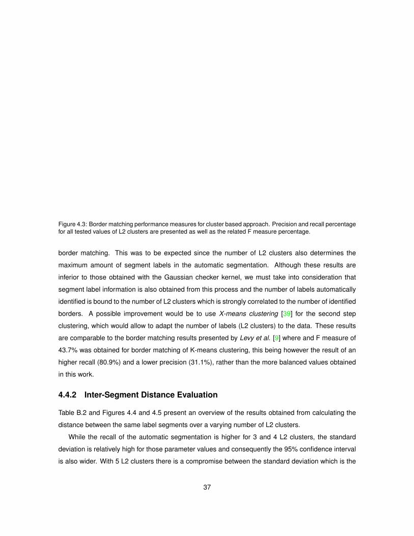
Figure 4.3: Border matching performance measures for cluster based approach. Precision and recall percentagefor all tested values of L2 clusters are presented as well as the related F measure percentage.

border matching. This was to be expected since the number of L2 clusters also determines the

maximum amount of segment labels in the automatic segmentation. Although these results are

inferior to those obtained with the Gaussian checker kernel, we must take into consideration that

segment label information is also obtained from this process and the number of labels automatically

identified is bound to the number of L2 clusters which is strongly correlated to the number of identified

borders. A possible improvement would be to use X-means clustering [39] for the second step

clustering, which would allow to adapt the number of labels (L2 clusters) to the data. These results

are comparable to the border matching results presented by Levy et al. [9] where and F measure of

43.7% was obtained for border matching of K-means clustering, this being however the result of an

higher recall (80.9%) and a lower precision (31.1%), rather than the more balanced values obtained

in this work.

4.4.2 Inter-Segment Distance Evaluation

Table B.2 and Figures 4.4 and 4.5 present an overview of the results obtained from calculating the

distance between the same label segments over a varying number of L2 clusters.

While the recall of the automatic segmentation is higher for 3 and 4 L2 clusters, the standard

deviation is relatively high for those parameter values and consequently the 95% confidence interval

is also wider. With 5 L2 clusters there is a compromise between the standard deviation which is the

37

L2 clusters 3 4 5 6 7 10

Average correct labels GT 5.02 5.02 5.02 5.02 5.02 5.02Average correct labels AS 2.28 2.97 3.68 4.23 4.98 7.12Average existing labels GT 5.68 5.68 5.68 5.68 5.68 5.68Average existing labels AS 3 4 5 6 7 10Recall GT % 88.27 88.27 88.27 88.27 88.27 88.27Recall AS % 75.96 74.17 73.67 70.56 71.19 71.17Standard deviation recall GT % 12.97 12.97 12.97 12.97 12.97 12.97Standard deviation recall AS % 23.84 20.9 16.14 17.05 17.49 14.89Ratio recall AS to recall GT 0.86 0.84 0.83 0.8 0.81 0.81

Table 4.5: Self-similarity distance evaluation results for the segmentations obtained with the range of testedL2 cluster values. Note that GT (ground truth) values were included for comparison with the AS (automaticsegmentation) results. A more complete set of results can be found in Table B.2 in Appendix A

Figure 4.4: Recall percentage from the self-similarity distance evaluation, presented for the range of tested L2clusters.

lowest of the result set - 7.7% lower than for 3 L2 Clusters - while there is only an 2.29% decrease

in recall. From Figure 4.5, it is possible to conclude that with 5 L2 clusters the total number of

labels for the automatic segmentation is close to the average number of correct labels in the ground

truth segmentation. Although the average correct labels retrieved from the automatic segmentation

with 5 L2 clusters (3.68) is still lower than the corresponding average correct GT labels (5.02), from

these considerations and in light of the results in Section 4.4, which shows that the clustering based

border matching achieves better results with 5L2 clusters, the use of 5 L2 clusters for this type of

38

Figure 4.5: Average total labels and correct labels from GT and AS for the range of tested L2 clusters.

segmentation seems to be a balanced choice, given the nature of the evaluated corpus and of the

features used. A complete list of all the songs sorted by recall can be found in Appendix B, FigureB.3.

4.4.3 Empirical Evaluation of the Cluster Based Segmentation Results

Another important aspect of the evaluation is the actual empirical human perception of the results of

the segmentation. While from the previous Sections 4.4.1 and 4.4.2, a cluster based segmentation

using 5 L2 clusters would seem to be a balanced choice for the evaluated corpus, from listening

to the automatic segmentations, it would seem otherwise that better automatic segmentations are

those that have a closer number of labels to those present in the ground truth. Follows an example

for the song “Wonder Wall” from the musical band Oasis, also included in the corpus, where the

segmentations for different number of L2 clusters are presented as well as the ground truth, Figures

4.6, 4.7, 4.8 and 4.9.

39

Figure 4.6: Segmentation view for “Wonder Wall” from Oasis, with the 3 L2 clusters (Labels) retrieved. Thenumbers in the upper left corner of the segments are the label tags, and a timeline in minutes is also shown.



Figure 4.9: Segmentation view for “Wonder Wall” from Oasis using the ground truth segmentation.The numbersin the upper left corner of the segments are the label tags, and a time-line in minutes is also shown.

In these examples, 7 L2 clusters provide results that are more consistent to a listener. Visually,

it is also easier to identify correspondences between segments or groups of segments in the 7 L2

cluster segmentation and the ground truth, e.g. segment with label 2 in the ground truth segmentation

seems to be explained by segments labelled 4 and 2 of the 7 L2 cluster segmentation. Again, this

suggests that a variable L2 cluster segmentation such as X-means clustering [39] could be used to

improve results.

40

4.5 Evaluation of Distance Measures

Using the method described in Section 4.2.3 and the corpus formed as stated in Section 4.1 the four

cluster distance measures described in Section 2.4 were used with thee different numbers of clusters

to produce the overall results that can be found in tables 4.6 and figures 4.10. Mode detailed results,

contained the success scores per category can be found in Appendix C, Tables C.2, C.3 and C.4 and

Figures C.1, C.2 and C.3.

Number of Clusters 1 10 20

Cluster Covariance % 20 23.2 22.4Euclidean Distance % 97.6 78.4 84.8KL Multivariate Gaussian % 66.4 49.6 48.8Average KL Single Gaussian % 84 60 59.2

Table 4.6: Overview of the tested cluster distance measures versus the number of clusters used. The resultsare expressed in the score calculated as mentioned in Section 4.2.3 and expressed in terms of percentage.

Figure 4.10: Overview of the tested cluster distance measures versus the number of clusters used.

A relevant observation that can be made from this small scale evaluation was that the Euclidean

cluster distance obtained the highest score in all evaluations. This is in sharp contrast with the

covariance distance measure, and suggests that the location of the cluster centres has a much

41

higher discriminating capability that the variance of the point distribution within each cluster - Note

that the covariance cluster distance measure normalizes all the points in a cluster by their mean. The

Cluster KL based approaches, perform competitively to the euclidean distance but are not able to

match it in any evaluated category.

Also noteworthy is that an increased number of clusters will not necessarily result in a better

score. Again the Euclidean cluster distance measure, seems to counter this tendency since for 20

clusters the success score is 6.4% better that with 10 clusters, although not achieving the same result

obtained with just 1 cluster. From other small scale experiments, it was determined that good results

can be achieved with an Euclidean distance as a cluster distance measure of up to 80 clusters.

From other small scale evaluations, it was determined that while clustering of songs features can

produce viable classifications, the fact that these classification rely on a random component - the

“seeds” used to obtain the cluster centres - adds “noise” do the distance measures retrieved using

this type of classification. This means that two distinct comparisons of the same two songs might not

always return the same distance value, due to different clustering outcomes, which is not desirable

if the aim is to obtain a reproducible distance measure, specially in a larger corpus where several

songs might have very close distances from each other. This being the case, different approaches

using Support Vector Machines (SVM) such as Ellis et al. [16] or Hidden Markov Models (HMM) as

in Levy et al. [9], than do not rely on random components, should be considered for future work.

42

Chapter 5

Conclusion

5.1 Result Summary and Discussion

The segmentation results can be summarized as follows:

• The border matching using a Gaussian Checker Kernel resulted in a maximum F measure of

62%, which is within the range of the values obtained from previous works like Ong [14] and

Peiszer [12] using the same algorithm.

• The border matching using a clustering-based segmentation approach resulted in low values

of F measure of only 46%. However, this is still higher that the results reported in Levy et al. [9]

for experiments using similar algorithms.

• The evaluation of the segmentation through the use of a distance measure, was an attempt

to establish a utility measure of the automatic segmentation produced by the cluster-based

segmentation. With the criteria used, it was shown that while a manually annotated corpus

contains approximately 88% of similar segments that are annotated with the same label, the

cluster-based segmentation was able to identify segments that are between 71% and 76%

similar among those with the same label.

• Empirical listening of the music segmentations produced also proved that the results of the

automatic segmentation were positive, in particular when the number of L2 clusters used was

closer to the number of manually annotated labels in a song.

For the music distance measures, a result summary follows:

• The Euclidean distance between clusters was the most successful measure employed. This

indicates that the centre of feature space, defined by each category of songs evaluated, was

itself a discriminator of the category, which was more evident in the single cluster experiments.

43

• In the task of finding the 5 closest songs from the biased corpus, experiments with multiple

clusters obtained worse results than using just 1 cluster. This indicates that an increased

number of clusters will not necessarily hold better results. The Euclidean cluster distance

measure, seems to counter this tendency, since for 20 clusters the success score is 6.4%

better that with 10 clusters, although it is still lower than the score obtained with just 1 cluster.

• The covariance cluster distance measure obtained consistently bad results, since the average

(centre of the cluster) is subtracted in it’s calculus. This is coherent with the conclusions above.

• The average KL divergence of a single Gaussian PDF per feature distance measure, when

employed to evaluate similarity among segments supposedly similar according to manual an-

notations, proved to return consistent results both empirically, by identifying incorrectly manu-

ally annotated segments, and in the context of the evaluation of the automatic segmentation by

comparison with the ground truth segmentation.

• The KL divergence using a multivariate Gaussian as a PDF for modelling the clusters held

positive results, but worse than those obtained by modelling each feature as a Gaussian in-

dependently. This indicates that a combination of the later might be a more adequate PDF to

model the feature space.

• The Earth Mover’s distance measure implementation was validated since as show, with the

exception the covariance cluster distance measure, all others produced positive scores with

more that 1 cluster, and in the case of the Euclidean cluster distance, 20 clusters held better

results than 10 clusters, as expected.

• While the KL divergence based strategies had generally lower performance that the Euclidean

distance, it is not clear that this advantage will hold in a more heterogeneous corpus, and for

an higher number of clusters. However, it is clear that the Euclidean distance and KL based

methods held positive results.

5.2 Future Work

From the author’s experience, future work and improvements to Shkr should be concentrated in:

• Moving the feature extraction inside the code base of Shkr, or at least under the control of the

Shkr code base, to allow for the integration of beat and metric detection.

44

• Optimizing the available functionality by resorting to feature testing and selection, and possi-

bly include PCA among the available tools to reduce the dimensionality of the features (when

applicable).

• Playlist retrieval and optimization strategies are desirable, and will greatly improve the useful-

ness of the implemented distance measures, specially in the context of a content recommen-

dation system.

• Other Classifiers such as HMM or SVM should be included as well, since K-Means clustering

does not always converge, and results rely on random seeds, which can cause inconsistencies,

specially song distance measures. The use of other clustering types, such as X-Means [39],

could also hold improvements, specially for segmentation, where the most appropriate number

of clusters could be automatically determined.

5.3 Objectives versus Challenges

It is the author’s opinion that these results validate the implementations, show the applicability of the

strategies used, and therefore the objectives of this work were accomplished. Although there were

several tasks being approached and few task-specific optimizations were introduced, the results were

still comparable to those obtained from other authors. Shkr is still a developing project, and while

for segmentation tasks applicable results can already be obtained, for the distance measures more

research and testing is necessary, and hence the small scale of the test performed in the scope of

this thesis.

However, a considerable code base with numerous useful resources and a flexible design that

can support several tasks in MIR was built, and while the effort was not invested in highly desirable

improvements such as feature selection, or beat detection integration, foundations were laid that can

help leverage such functionality in future.

45

References

[1] Howes, F. Man Mind and Music. Marin Secker & Warbug LTD., 1948.

[2] Mirex. http://www.music-ir.org/mirex/wiki/MIREX_HOME (Visited on 2010/09/12).

[3] Ismir. http://www.ismir.net/ (Visited on 2010/09/12).

[4] Schnitzer, D. Mirage, high-performance music similarity computation and automatic playlist

generation. Master’s thesis, Vienna University of Technology, 2007.

[5] Midomi. http://www.midomi.com/ (Visited on 2010/09/12).

[6] Paulus, J., Klapuri, A. Music Structure Analysis by Finding Repeated Parts. proceedings of

AMCMM 06, pages 59–67, 2006.

[7] Lee, k. Automatic Chord Recognition Using Enhanced Pitch Class Profile. proceedings of

International Computer Music Conference, 2006.

[8] Childers D. G., Skinner D. P., Kemerait R. C. The Cepstrum, A guide to Processing. proceedings

of IEEE, 65(10):1428–1423, 1977.

[9] Levy, M., Sandler M. Structural Segmentation of Musical Audio by Constrained Clustering. IEEE

Ttransactions on Audio, Speech, and Language processing, 16(2), 2008.

[10] MPEG-7 Standard ISO/IEC 15938-4:2002. http://www.chiariglione.org/mpeg/standards/

mpeg-7/mpeg-7.htm (Visited on 2010/10/10).

[11] Logan, B., Salomon, A. A Music Similarity Function Based on Signal Analysis. Multimedia and

Expo, 2001. ICME 2001. IEEE International Conference, pages 745–748, 2001.

[12] Peiszer, E. Automatic Audio Segmentation: Segment Boundary and Structuzre Detection in

Popular Music. Master’s thesis, Institut fur Softwaretechnik und Interaktive Systeme, 2007.

[13] Foote, J., Cooper, M. Media segmentation using self-similarity decomposition. IEEE ICME,

2003.

46

http://www.music-ir.org/mirex/wiki/MIREX_HOME

http://www.ismir.net/

http://www.midomi.com/

http://www.chiariglione.org/mpeg/standards/mpeg-7/mpeg-7.htm

http://www.chiariglione.org/mpeg/standards/mpeg-7/mpeg-7.htm

[14] Ong, B. S. Towards Automatic Music Structural Analysis: Identifying Characteristic Within-Song

Excerpts in Popular Music. PhD thesis, Universitat Pompeu Fabra, 2005.

[15] Foote, J. Automatic Audio Segmentation using a measure of audio novelty. proceedings of

IEEE, 2000.

[16] Ellis, D.,Mandel, M. Song-level features and support vector machines for music classification.

In ISMIR 2005, pages 594–599, 2005.

[17] Erickson, R. Sound Structure in Music. University of California Press, 1975.

[18] Hidden Markov Model Toolkit. http://http://htk.eng.cam.ac.uk/ (Visited on 2010/09/03).

[19] Huang, X., Acero, A., Won, H. Spoken Language Processing. Prentice Hall, 2001.

[20] Miranda, M. Trabalho do Miguel. 2009.

[21] Sonic Visualiser. http://www.sonicvisualiser.org/ (Visited on 2008/09/28).

[22] Rubner, Y., Tomasi, C., Guibas, L. J. The Earth Mover’s Distance as a Metric for Image Retrieval.

International Journal of Computer Vision, 40(2), pages 99–121, 2000.

[23] lpsolve - Mixed Integer Linear Programming (MILP) solver. http://lpsolve.sourceforge.net/

5.5/ (Visited on 2010/09/03).

[24] Marques, J. S. Reconhecimento de Padroes: metodos estatısticos e neuronais. IST press,

1999.

[25] Vorbis.com. http://www.vorbis.com/ (Visited on 2010/09/28).

[26] FLAC - Free Lossless audio codec. http://flac.sourceforge.net/ (Visited on 2010/09/28).

[27] SoX - Sound eXange. http://sox.sourceforge.net/ (Visited on 2010/09/28).

[28] Department of Music from the University of Jyvaskyla . http://www.jyu.fi/hum/laitokset/

musiikki/en/research/coe/materials/mirtoolbox (Visited on 2010/10/08).

[29] Eigen Wiki. http://eigen.tuxfamily.org/index.php?title=Main_Page (Visited on

2010/09/12).

[30] The GNU C++ Library Documentation. http://gcc.gnu.org/onlinedocs/libstdc++ (Visited

on 2010/09/12).

47

http://http://htk.eng.cam.ac.uk/

http://www.sonicvisualiser.org/

http://lpsolve.sourceforge.net/5.5/

http://lpsolve.sourceforge.net/5.5/

http://www.vorbis.com/

http://flac.sourceforge.net/

http://sox.sourceforge.net/

http://www.jyu.fi/hum/laitokset/musiikki/en/research/coe/materials/mirtoolbox

http://www.jyu.fi/hum/laitokset/musiikki/en/research/coe/materials/mirtoolbox

http://eigen.tuxfamily.org/index.php?title=Main_Page

http://gcc.gnu.org/onlinedocs/libstdc++

[31] Tzanetakis, G., Bray, S. Implicit patching for dataflow-based audio analysis and synthesis. In

Proceedings of the 2005 International Computer Music Conference, 2005.

[32] Marsyas - Musical Analysis, Retrieval and Synthetisis for Audio Signals. http://marsyas.info/

(Visited on 2010/09/03).

[33] Eckel, B. Thinking in Patterns - Problem-Solving Techniques Using Java, Revision 0.9. Uni-

versity of California Press, 2003. Online publication at http://www.mindview.net/Books/

TIPatterns/ (Visited on 2010/09/03).

[34] Xerces C++ XML Parse. http://xerces.apache.org/xerces-c/ (Visited on 2010/09/03).

[35] David, A., Vassilvitskii, S. k-means++: The advantages of careful seeding. 2006.

[36] Vienna University of Technology - Music Information Retrieval. http://www.ifs.tuwien.ac.

at/mir/audiosegmentation.html (Visited on 2010/09/28).

[37] Chai, W. Structural Analysis of Musical Signals for Indexing and Thumbnailing. Proceedings of

the Joint Conference on Digital Libraries, pages 27–24, 2003.

[38] Logan, B., Ellis D.P.W., Barenzweig A. Toward evaluation techniques for music similarity. IEEE

ICME, 2003.

[39] Pelleg, D., Moore, A. X-means: Extending the K-means with Efficient Estimation of the Number

of Clusters. In Proceedings of the 17th International Conf. on Machine Learning, 2000.

48

http://marsyas.info/

http://www.mindview.net/Books/TIPatterns/

http://www.mindview.net/Books/TIPatterns/

http://xerces.apache.org/xerces-c/

http://www.ifs.tuwien.ac.at/mir/audiosegmentation.html

http://www.ifs.tuwien.ac.at/mir/audiosegmentation.html

Appendix A

Border Matching Results fromGaussian Checker Kernel Matrix andClustering Based Segmentation

Gaussian standard Deviation 3 6 12 18 24 30 36Checker size 5 10 20 30 40 50 60Total Number of songs 61 61 61 61 61 61 61Total annotated borders 842 842 842 842 842 842 842Total Correct Borders 600 659 624 556 449 461 424Total Identified Borders 1599 1494 1223 992 857 769 719Average borders per song 13.80 13.80 13.80 13.80 13.80 13.80 13.80Average correct borders per song 9.84 10.80 10.23 9.11 8.18 7.56 6.95Average matched borders per song 26.21 24.49 20.05 16.26 14.05 12.61 11.78Average Precision % 39.41 45.56 53.45 57.78 59.93 60.71 59.98Precision standard deviation % 14.61 16.42 18.66 20.83 21.29 19.98 19.59Precision 95.0% confidence interval 3.67 4.12 4.68 5.23 5.34 5.01 4.92Average Recall % 72.82 79.09 76.08 67.67 60.57 56.25 52.23Recall standard devitation % 17.61 17.21 15.03 15.98 16.16 16.33 15.83Recall 95.0% confidence interval 4.42 4.32 3.77 4.01 4.06 4.10 3.97Correlation precision and recall 0.58 0.51 0.39 0.40 0.46 0.45 0.48Correlation annotated and identified 0.56 0.54 0.46 0.43 0.42 0.45 0.46Correlation identified and correct 0.43 0.47 0.35 0.39 0.45 0.51 0.51F measure % 51 57 62 62 60 58 55

Table A.1: Border matching performance measures for the range of tested standard Deviation and Size of theGaussian checker kernel.

A1

L2 clusters 3 4 5 6 7 10L1 clusters 80 80 80 80 80 80Cluster histogram size 60 60 60 60 60 80Total number of songs 61 61 61 61 61 61Total annotated borders 842 842 842 842 842 842Total correct borders 320 349 412 431 458 517Total identified borders 626 831 1015 1175 1278 1557Average borders per song 13.80 13.80 13.80 13.80 13.80 13.80Average correct borders per song 5.25 5.72 6.75 7.07 7.51 8.48Average matched borders per song 10.26 13.62 16.64 19.26 20.95 25.52Average precision % 53.49 45.16 43.84 39.61 37.61 34.32Precision standard deviation % 18.28 18.11 16.01 15.69 13.35 12.59Precision 95.0% confidence interval 4.59 4.54 4.02 3.94 3.35 3.16Average recall % 39.09 42.6 50.27 53.16 56.49 62.25Recall standard deviation % 14.08 14.14 14.41 16.38 17.63 14.9Recall 95.0% confidence interval 3.53 3.55 3.62 4.11 4.43 3.74Correlation precision and recall 0.22 0.23 0.24 0.43 0.23 0.26Correlation annotated and identified 0.22 0.17 0.28 0.16 0.18 0.13Correlation identified and correct 0.45 0.39 0.4 0.16 0.34 0.2F measure % 45 43 46 45 45 44

Table A.2: Border matching performance measures for cluster based approach for the range of tested L2 clustervalues

A2

The_Clash_-_Should_I_Stay_or_Should_I_Go

Alanis_Morissette_-_Thank_You

Madonna-Like_a_virgin

The_Crystal_Method_-_Born_Too_Slow

The_Monkees_-_Words

Oasis_-_Wonderwall

Prince_-_Kiss

Seal_-_Crazy

Chumbawamba_-_Thubthumping

Simply_Red_-_Stars

Deus_-_suds_and_soda

Beatles_-_Dont_Bother_Me

Beatles_-_Till_There_Was_You

Spice_Girls_-_Wannabe

Beatles_-_I_saw_her_standing_there

Beatles_-_You_Really_Got_A_Hold_On_Me

Cranberries_-_Zombie

The_Beatles_-_Within_You_Without_You

Britney_Spears_-_Hit_Me_Baby_One_More_Time

Alanis_Morissette_-_08_-_Head_Over_Feet

The_Beatles_-_A_Day_In_The_Life

The_Beatles_-_Lucy_In_The_Sky_With_Diamonds

Beatles_-_Hold_Me_Tight

Beatles_-_Misery

Beatles_-_Not_A_Second_Time

Beatles_-_Roll_Over_Beethoven

The_Beatles_-_Getting_Better

Beatles_-_It_Wont_Be_Long

Bjork_-_Its_Oh_So_Quiet

Beastie_Boys_-_Intergalactic

REM_-_Drive

Nora_Jones_-_Lonestar

The_Beatles_-_Good_Morning_Good_Morning

Wise_Guys_-_Powerfrau

Chicago_-_Old_Days

Beatles_-_Little_Child

Beatles_Anna_go_to

Sinhead_O_Connor_-_Nothing_compares_to_you

The_Beatles_-_Shes_Leaving_Home

Beatles_-_Please_Mister_Postman

Black_Eyed_Peas_-_Cali_To_New_York

Nirvana_-_Smells_like_teen_spirit

The_Beatles_-_With_A_Little_Help_From_My_Friends

A-HA_-_Take_on_me

Portishead_-_Wandering_star

Beatles_-_All_My_Loving

The_Beatles_-_Being_For_The_Benefit_Of_Mr_Kite

The_Beatles_-_Sgt_Peppers_Lonely_Hearts_Club_Band

Beatles_-_I_Wanna_Be_Your_Man

The_Beatles_-_Lovely_Rita

Beatles_-_Money

Nick_Drake_-_Northern_Sky

Radiohead_-_Radiohead_-_Creep_Original_Ve

Gloria_Gayner-I_Will_Survive

Wise_Guys_-_Kinder

Apollo_440_-_Stop_The_Rock

Beatles_-_All_Ive_Got_To_Do

Beatles_-_Devil_In_Her_Heart

The_Beatles_-_Fixing_A_Hole

The_Beatles_-_Sgt_Peppers_Lonely_Hearts_reprise

The_Beatles_-_When_Im_Sixty-Four

0 10 20 30 40 50 60 70 80 90 100

Gaussian Checker Kernel Full Corpus Border Matching 20 frames side size, stdandard deviation of 12

RecallPrecision

Measure Percentage

Figure A.1: List songs with corresponding recall and precision, sorted by recall for the a Gaussian matrix side of20 and a Gaussian standard deviation of 12

A3




The_Monkees_-_Words

REM_-_Drive

Oasis_-_Wonderwall







Seal_-_Crazy




Beatles_-_Misery







Beatles_Anna_go_to




Prince_-_Kiss





A-HA_-_Take_on_me


Simply_Red_-_Stars












Chicago_-_Old_Days

Wise_Guys_-_Kinder









Beatles_-_Money





0 10 20 30 40 50 60 70 80 90 100


RecallPrecision

Measure Percentage


A4



The_Monkees_-_Words





REM_-_Drive





Beatles_Anna_go_to

Beatles_-_Misery


Oasis_-_Wonderwall




Seal_-_Crazy




Wise_Guys_-_Kinder









Simply_Red_-_Stars









A-HA_-_Take_on_me



Prince_-_Kiss






Beatles_-_Money




Chicago_-_Old_Days







0 10 20 30 40 50 60 70 80 90 100


RecallPrecision

Measure Percentage


A5






Seal_-_Crazy




Prince_-_Kiss






Beatles_-_Misery






Beatles_Anna_go_to



A-HA_-_Take_on_me






REM_-_Drive



Chicago_-_Old_Days





Beatles_-_Money






Oasis_-_Wonderwall



Simply_Red_-_Stars


Wise_Guys_-_Kinder






The_Monkees_-_Words






0 10 20 30 40 50 60 70 80 90 100

Clustering Based Border Matching 5 cluster L2, 80 clusters L1

RecallPrecision

Measure Percentage

Figure A.4: List songs with corresponding recall and precision, sorted by recall for the clustering based segmen-tation using 5 clusters L2 and 80 clusters L1.

A6

Appendix B

Segment Similarity Results of the KLDivergence of a Single Gaussian perFeature Distance measure

B7

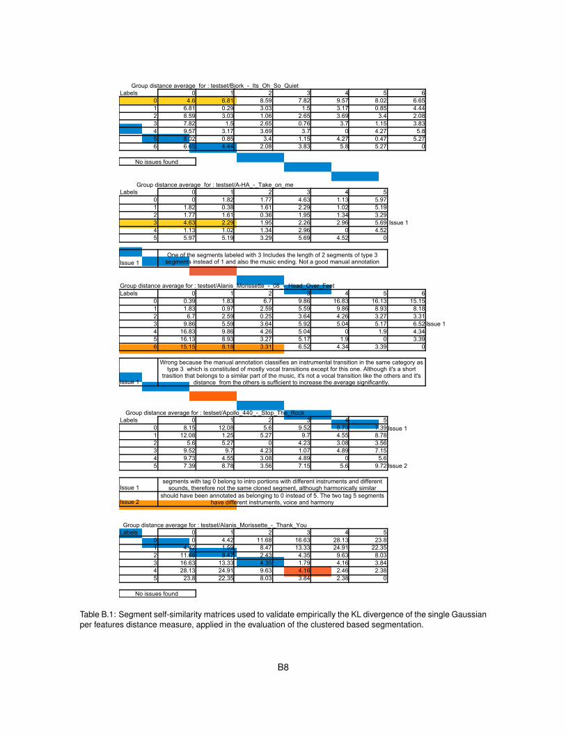
Labels 0 1 2 3 4 5 60 4.6 6.81 8.59 7.82 9.57 8.02 6.651 6.81 0.29 3.03 1.5 3.17 0.85 4.442 8.59 3.03 1.06 2.65 3.69 3.4 2.083 7.82 1.5 2.65 0.76 3.7 1.15 3.834 9.57 3.17 3.69 3.7 0 4.27 5.85 8.02 0.85 3.4 1.15 4.27 0.47 5.276 6.65 4.44 2.08 3.83 5.8 5.27 0

No issues found

Labels 0 1 2 3 4 50 0 1.82 1.77 4.63 1.13 5.971 1.82 0.38 1.61 2.29 1.02 5.192 1.77 1.61 0.36 1.95 1.34 3.293 4.63 2.29 1.95 2.26 2.96 5.69 Issue 14 1.13 1.02 1.34 2.96 0 4.525 5.97 5.19 3.29 5.69 4.52 0

Issue 1

Labels 0 1 2 3 4 5 60 0.39 1.83 6.7 9.86 16.83 16.13 15.151 1.83 0.97 2.59 5.59 9.86 8.93 8.182 6.7 2.59 0.25 3.64 4.26 3.27 3.313 9.86 5.59 3.64 5.92 5.04 5.17 6.52 Issue 14 16.83 9.86 4.26 5.04 0 1.9 4.345 16.13 8.93 3.27 5.17 1.9 0 3.396 15.15 8.18 3.31 6.52 4.34 3.39 0

Issue 1

Labels 0 1 2 3 4 5

Issue 10 8.15 12.08 5.6 9.52 9.73 7.391 12.08 1.25 5.27 9.7 4.55 8.782 5.6 5.27 0 4.23 3.08 3.563 9.52 9.7 4.23 1.07 4.89 7.154 9.73 4.55 3.08 4.89 0 5.65 7.39 8.78 3.56 7.15 5.6 9.72 Issue 2

Issue 1

Issue 2

Labels 0 1 2 3 4 50 0 4.42 11.68 16.63 28.13 23.81 4.42 1.59 8.47 13.33 24.91 22.352 11.68 8.47 2.43 4.35 9.63 8.033 16.63 13.33 4.35 1.79 4.16 3.844 28.13 24.91 9.63 4.16 2.46 2.385 23.8 22.35 8.03 3.84 2.38 0

No issues found

Group distance average for : testset/Bjork_-_Its_Oh_So_Quiet

Group distance average for : testset/A-HA_-_Take_on_me

One of the segments labeled with 3 Includes the length of 2 segments of type 3 segments instead of 1 and also the music ending. Not a good manual annotation

Group distance average for : testset/Alanis_Morissette_-_08_-_Head_Over_Feet

Wrong because the manual annotation classifies an instrumental transition in the same category as type 3 which is constituted of mostly vocal transitions except for this one. Although it's a short

trasition that belongs to a similar part of the music, it's not a vocal transition like the others and it's distance from the others is sufficient to increase the average significantly.

Group distance average for : testset/Apollo_440_-_Stop_The_Rock

segments with tag 0 belong to intro portions with different instruments and different sounds, therefore not the same cloned segment, although harmonically similar

should have been annotated as belonging to 0 instead of 5. The two tag 5 segments have different instruments, voice and harmony

Group distance average for : testset/Alanis_Morissette_-_Thank_You

Table B.1: Segment self-similarity matrices used to validate empirically the KL divergence of the single Gaussianper features distance measure, applied in the evaluation of the clustered based segmentation.

B8

L2 clusters 3 4 5 6 7 10L1 clusters 80 80 80 80 80 80Cluster histogram size 60 60 60 60 60 80Total number of songs 61 61 61 61 61 61Total correct labels GT 301 301 301 301 301 301Total correct labels AS 139 178 221 254 299 427Total existing lables GT 341 341 341 341 341 341Total existing lables AS 183 240 300 360 420 600Average correct labels GT 5.02 5.02 5.02 5.02 5.02 5.02Average correct labels AS 2.28 2.97 3.68 4.23 4.98 7.12Average existing labels GT 5.68 5.68 5.68 5.68 5.68 5.68Average existing labels AS 3 4 5 6 7 10Recall % GT 88.27 88.27 88.27 88.27 88.27 88.27Recall % AS 75.96 74.17 73.67 70.56 71.19 71.17Standard deviation recall % GT 12.97 12.97 12.97 12.97 12.97 12.97Standard deviation recall % AS 23.84 20.9 16.14 17.05 17.49 14.89Confidence interval recall 95% GT 3.26 3.26 3.26 3.26 3.26 3.26Confidence interval recall 95% AS 5.98 5.24 4.05 4.28 4.39 3.74Ratio recall AS to recall GT 0.86 0.84 0.83 0.8 0.81 0.81

Table B.2: Self-similarity distance evaluation results for the segmentations obtained with the range of testedL2 cluster values. Note that GT (ground truth) values were included for comparison with the AS (automaticsegmentation) results.

B9



Prince_-_Kiss






Beatles_-_Misery







REM_-_Drive

Seal_-_Crazy







Wise_Guys_-_Kinder

A-HA_-_Take_on_me







Beatles_-_Money



















The_Monkees_-_Words




Beatles_Anna_go_to


Chicago_-_Old_Days


Oasis_-_Wonderwall

Simply_Red_-_Stars


0 10 20 30 40 50 60 70 80 90 100

Self Segment Similarity Matching GT vs AS with 5 Clusters L2 Recall ASRecall GT

Recall Percentage

Table B.3: Segment self-similarity results for all songs in the corpus, for an automatic segmentation using 5 L2clusters and sorted by the automatic segmentation’s recall. The inter-segment distance measure used was athe average of the KL divergence for each feature.

B10

Appendix C

Small Scale Evaluation of SongDistance Measure Results

Artist Album Song

Al Di Meola,Paco de Lucia,John McLaughlin The Guitar Trio La EstibaAl Di Meola,Paco de Lucia,John McLaughlin The Guitar Trio Beyond The MirageAl Di Meola,Paco de Lucia,John McLaughlin The Guitar Trio Midsummer NightAl Di Meola,Paco de Lucia,John McLaughlin The Guitar Trio Manha De CarnavalAl Di Meola,Paco de Lucia,John McLaughlin The Guitar Trio Letter From India

Bobby McFerrin Simple Pleasures Don’t Worry Be HappyBobby McFerrin Simple Pleasures All I WantBobby McFerrin Simple Pleasures Drive My CarBobby McFerrin Simple Pleasures Simple PleasuresBobby McFerrin Simple Pleasures Good Lovin

Iron Maiden The Number of the Beast The PrisonerIron Maiden The Number of the Beast 22 Acacia AvenueIron Maiden The Number of the Beast The Number Of The BeastIron Maiden The Number of the Beast InvadersIron Maiden The Number of the Beast Children Of The Damned

Mozart Six German Dances track 1Mozart Six German Dances track 2Mozart Six German Dances track 3Mozart Six German Dances track 4Mozart Six German Dances track 5

Transmissions Juno Reactor High Energy ProtonsTransmissions Juno Reactor The HeavensTransmissions Juno Reactor Luna-ticTransmissions Juno Reactor ContactTransmissions Juno Reactor Acid Moon

Table C.1: List of songs which compose the small scale evaluation corpus of distance measures.

C11

A B C D E Total

Cluster Covariance 16% 12% 28% 28% 16% 20%Euclidean Distance 96% 100% 100% 96% 96% 97.6%KL Multivariate Gaussian 68% 88% 64% 52% 60% 66.4%Avgerage KL of Gaussians 92% 72% 96% 84% 76% 84%

Table C.2: Results of the different cluster distance measures for all of the corpus categories with only 1 cluster incomparison which implies that the Earth Mover’s distance is not used. The results are expressed in percentageusing the the success score as mentioned in 4.2.3

Figure C.1: Comparison of the tested cluster distance measures using 1 cluster.

A B C D E Total

Cluster Covariance 28% 12% 24% 28% 24% 23.2%Euclidean Distance 76% 60% 100% 76% 80% 78.4%KL Multivariate Gaussian 28% 32% 88% 52% 48% 49.6%Avgerage KL of Gaussians 40% 52% 92% 56% 60% 60%

Table C.3: Results of the different cluster distance measures for all of the corpus categories with 10 clustersclusters in comparison. The results are expressed in percentage using the the success score as mentioned in4.2.3

C12

Figure C.2: Comparison of the tested cluster distance measures using 10 clusters.

A B C D E Total

Cluster Covariance 16% 24% 20% 20% 32% 22.4%Euclidean Distance 88% 64% 100% 80% 92% 84.8%KL Multivariate Gaussian 40% 40% 68% 44% 52% 48.8%Avgerage KL of Gaussians 52% 48% 76% 52% 68% 59.2%

Table C.4: Results of the different cluster distance measures for all of the corpus categories with 20 clustersclusters in comparison. The results are expressed in percentage using the the success score as mentioned in4.2.3

C13

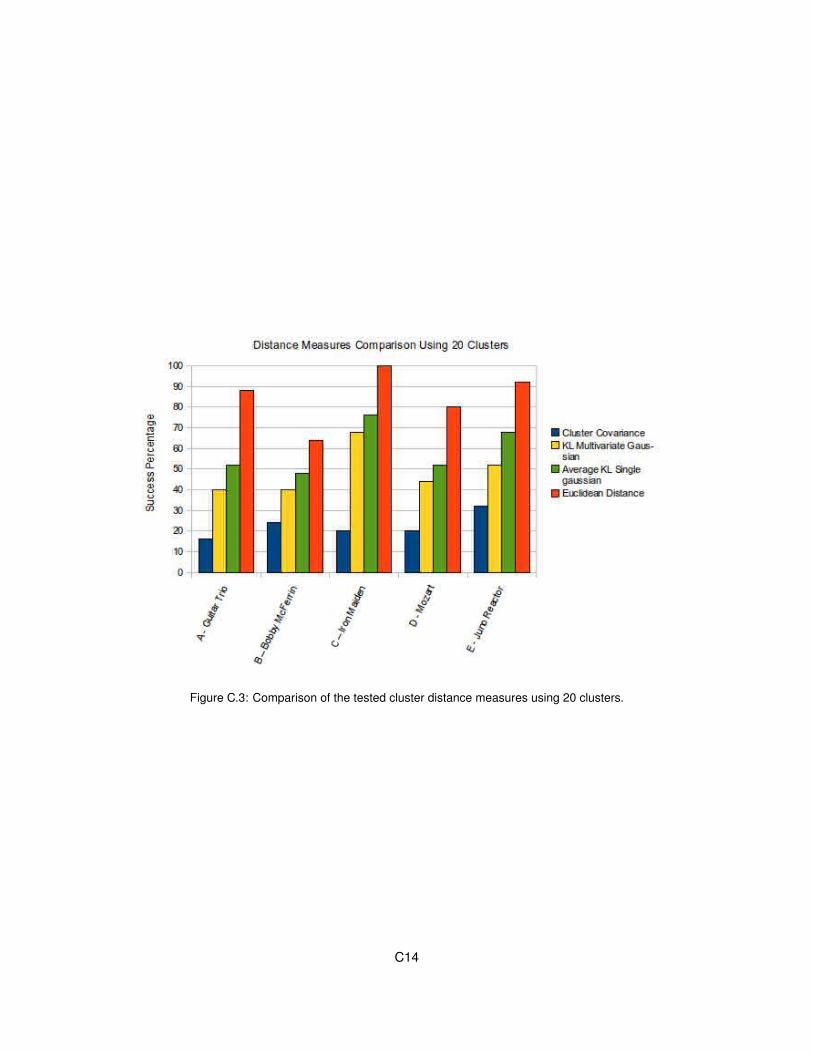
Figure C.3: Comparison of the tested cluster distance measures using 20 clusters.

C14

Music Information Retrieval Engenharia Informática e de ...

Documents

Transcript of Music Information Retrieval Engenharia Informática e de ...