
Murat Alaboz Dynamic Identification and Modal Updating of S ...
106
Murat Alaboz Dynamic Identification and Modal Updating of S.Torcato Church Portugal I 2009
-
Upload
khangminh22 -
Category
Documents
-
view
2 -
download
0
Transcript of Murat Alaboz Dynamic Identification and Modal Updating of S ...

Murat Alaboz
Dynamic Identification andModal Updating of S.TorcatoChurch
Portugal I 2009

Dynamic Identification and Modal Updating of S. Torcato Church M.Alaboz
Erasmus Mundus Programme ADVANCED MASTERS IN STRUCTURAL ANALYSIS OF MONUMENTS AND HISTORICAL CONSTRUCTIONS i
DECLARATION
Name: Murat ALABOZ
Email: [email protected]
Title of the
Msc Dissertation:
Dynamic Identification and Modal Updating of S.Torcato Church
Supervisor(s): Luis F. Ramos
Year: 2008 / 2009
I hereby declare that all information in this document has been obtained and presented in accordance
with academic rules and ethical conduct. I also declare that, as required by these rules and conduct, I
have fully cited and referenced all material and results that are not original to this work.
I hereby declare that the MSc Consortium responsible for the Advanced Masters in Structural Analysis
of Monuments and Historical Constructions is allowed to store and make available electronically the
present MSc Dissertation.
University: University of Minho
Date: June 2009
Signature: ___________________________

M.Alaboz Dynamic Identification and Modal Updating of S. Torcato Church
Erasmus Mundus Programme ii ADVANCED MASTERS IN STRUCTURAL ANALYSIS OF MONUMENTS AND HISTORICAL CONSTRUCTIONS

Dynamic Identification and Modal Updating of S. Torcato Church M.Alaboz
Erasmus Mundus Programme ADVANCED MASTERS IN STRUCTURAL ANALYSIS OF MONUMENTS AND HISTORICAL CONSTRUCTIONS iii
ACKNOWLEDGEMENTS
When finishing a journey, a journey of science, a journey of cultures and friendship, I would like to
thank everybody who was a part of each step of this master program. When leaving a tiring but
precious times behind, I will keep the entire valuable words, smiles of our professors and friends not
only regarding to the academic studies but life.
It is also a necessity for me to mention their names who guided me for a endless way of interest, the
issue of historical structures and conservation; Prof. Kamuran Öztekin from Kocaeli UIniversity and all
members of Civil Engineering Department.
For their academic support and leading advices during my previous master study in Istanbul Technical
University, I would like to thank to Prof. Zeynep Ahunbay, Ast. Prof. Gulsun Tanyeli and all the
members of the Restoration Department, distinctively to Ast. Umut Almac who informed me about
SAHC master program and courage me and to Prof. Gorun Arun from Yıldız Technical University for
her special supervision.
I want to express my gratitude to SAHC consortium for providing me a scholarship for the tuition fee to
participate in the program.
During the master program, for their invaluable support and endless understanding, I would like to
thank to all members of Civil Engineering Departments of University of Minho and University of
Padova, peculiarly to my supervisor Ast. Prof. Luis Ramos, Flippo Casarin, Prof.Pere Roca, Prof.
Paulo Lorenco and the others who I can not mention here.
Rafael Aguliar for his patience and generosity, being ready to answer all my questions and Alberto
who became a member of our dynamic test team and worked more than us, without their presence
those couldn’t be done.
Beside the academic works, three people who deal with our endless demands, Sandra Pereira, Dora
Coelho and Elisa Trovo merit very special thanks.
For the time we spent together and sharing I would like to thank to all my colleagues in the program.
They deserve a special thank who were the member of our large family in Guimaraes, On Yee Lee,
Ziba Sharafi, Fusun Ece Ferah, Alejandro Trulias, Visar Slhaku and Habtamu Bogale.

M.Alaboz Dynamic Identification and Modal Updating of S. Torcato Church
Erasmus Mundus Programme iv ADVANCED MASTERS IN STRUCTURAL ANALYSIS OF MONUMENTS AND HISTORICAL CONSTRUCTIONS
Tibebu Birhane has to be called as a special friend and even more, more than a brother. Thanks to
him for his existence, his energy, his love, his curiosity and enthusiasm that made me smile every
time, cause to alter difficulties and shows different perspectives,
Thanks to my family, for their great love and for being with me every time regardless from time and
place. Kıvanc İlhan, whom I can’t distinct from a brother, thanks to him for our endless discussions
and our unique humor.
And my sister Müge… I leave her name with dots as difficult as to describe a piece of my soul… It was
the most difficult part of the master just to be far from her.

Dynamic Identification and Modal Updating of S. Torcato Church M.Alaboz
Erasmus Mundus Programme ADVANCED MASTERS IN STRUCTURAL ANALYSIS OF MONUMENTS AND HISTORICAL CONSTRUCTIONS v
ABSTRACT
Considering the modern conservation criteria that demands minimum intervention and preservation of
historical constructions, the understanding of any damage phenomena and the seismic assessment
have significant importance. Any numerical model that is constructed for this purpose must represent
the existing properties and structural conditions. In that point, different non-destructive inspection
techniques are being used to provide local and global information.
Experimental dynamic identification techniques, which are generally based on the acceleration
records, allow obtaining natural frequencies, mode shapes and damping coefficients of a structural
system. These data represent the overall dynamic response of a structure as a result of its mechanical
properties that are generally unknown or difficult to obtain. If accurately estimated, the real response
of the structures under specified or unknown excitations can be used to tune numerical models.
In addition, dynamic measurements may be used for monitoring and for evaluating the changes of
dynamic response through time. Thus, dynamic monitoring can be used as a warning system
indicating possible damages on the structure or to check the efficiency of any intervention.
In this study, a dynamic identification analysis was carried on S. Torcato Church, in Guimarães,
Portugal. The church has significant structural problems, such as wide cracks on façade and tilting of
bell towers. Natural frequencies, mode shapes and damping coefficients were obtained by using
dynamic tests. The estimated dynamic properties were used to tune a finite element model by using
manual and robust modal updating algorithms.
In the experiments, ambient vibration records were taken within several setups and the collected data
was processed with different identification methods. The first four mode shapes of the structure were
accurately estimated. A finite element model was tuned to the experimental data. Modal updating
parameters were selected based on the frequency and model shape coherence. A non-linear solution
of combined updated parameters was carried out for the model updating analysis. All modification
steps and recommendations are presented in the light of difficulties faced during the dissertation
study.
Keywords: Historical constructions, masonry, dynamic identification, modal updating

M.Alaboz Dynamic Identification and Modal Updating of S. Torcato Church
Erasmus Mundus Programme vi ADVANCED MASTERS IN STRUCTURAL ANALYSIS OF MONUMENTS AND HISTORICAL CONSTRUCTIONS

Dynamic Identification and Modal Updating of S. Torcato Church M.Alaboz
Erasmus Mundus Programme ADVANCED MASTERS IN STRUCTURAL ANALYSIS OF MONUMENTS AND HISTORICAL CONSTRUCTIONS vii
RESUMO
Tendo em conta os princípios modernos sobre as intervenções e a preservação do património
histórico, a compreensão de todos fenómenos que provocam danos estruturais e o estudo da
vulnerabilidade sísmica das construções revestem-se de especial interesse. Qualquer modelo
numérico construído para esse fim deve reproduzir as propriedades e a resposta estrutural das
construções existentes. Diferentes ensaios não-destrutivos de inspecção e diagnóstico são
frequentemente usados para fornecer informação local e global das construções.
As técnicas experimentais para a identificação dinâmica, geralmente baseadas na medição de
acelerações, permitem obter as frequências naturais, modos de vibração e coeficientes de
amortecimento. Os dados obtidos representam a resposta global da estrutura, como resultado das
propriedades mecânicas que geralmente são desconhecidas ou difíceis de se obter por outra via.
Se estimada de forma precisa, a resposta dinâmica pode ser usada para ajustar modelos numéricos.
Adicionalmente, as vibrações podem ser usadas para a monitorização e para avaliação das
alterações dinâmicas ao longo do tempo. A monitorização dinâmica pode ser usada como um sistema
de alarme na detecção de danos estruturais ou como um sistema para avaliar a eficiência de
intervenções estruturais.
No presente estudo foi elaborada uma identificação dinâmica da igreja de S. Torcato, em Guimarães,
Portugal. A igreja apresenta um conjunto de anomalias estruturais, tais como fendas significativas nas
fachadas e a rotação das torres. Foram estimadas frequências naturais, modos de vibração e
coeficientes de amortecimento. Os parâmetros estimados foram usados para ajustar um modelo
numérico de elementos finitos, usando técnicas de ajuste manual e de ajuste robusto.
Nos ensaios experimentais, as vibrações naturais foram registadas em diferentes setups e os dados
foram processados com diferentes métodos de identificação modal. Os quatro primeiros modos de
vibração foram estimados de forma precisa. O modelo de elementos finitos foi ajustado aos primeiros
quatro modos. Os parâmetros de optimização estrutural foram seleccionados com base no ajuste das
frequências e modos de vibração. Uma solução não-linear para a optimização numérica foi também
utilizada. Todos os passos de análise e recomendações sobre as dificuldades encontradas são
também apresentados.
Palavras chave: Construções históricas, alvenaria, identificação dinâmica, optimização numérica

M.Alaboz Dynamic Identification and Modal Updating of S. Torcato Church
Erasmus Mundus Programme viii ADVANCED MASTERS IN STRUCTURAL ANALYSIS OF MONUMENTS AND HISTORICAL CONSTRUCTIONS

Dynamic Identification and Modal Updating of S. Torcato Church M.Alaboz
Erasmus Mundus Programme ADVANCED MASTERS IN STRUCTURAL ANALYSIS OF MONUMENTS AND HISTORICAL CONSTRUCTIONS ix
ÖZET
Minimum müdahaleyi ve mevcut yapım tekniklerinin korunmasını öngören modern koruma yaklaşımı
göz önünde bulundurulduğunda, yapıdaki hasarların doğru bir şekilde tespiti ve yapısal
hassasiyetinin değerlendirilmesi, uygun müdahele kararlarının verilmesinde büyük rol oynar. Bu
amaçla sıklıkla kullanılan sayısal modellemelerde, yapı mekanik özelliklerinin ve yapıya etki eden
kuvvetlerin doğru tanımlanması gerekmektedir. Yapısal özelliklerin belirlenmesinde, noktasal veya
bütünsel veri sağlayan hasarsız test yöntemleri kullanılmaktadr.
Genellikle ivme kayıtlarının işlenmesine dayanan dinamik tanımlama teknikleri ile yapının doğal
frekansı, mod şekilleri ve sönümlenme katsayıları elde edilmektedir. Buradan sağlanan veriler
yardımıyla geleneksel test yöntemleri ile berlirlenemeyen, yapının tüm mekanik özelliklerinin sonucu
olan yapı dinamik davranışı belirlenmektedir. Tanımlı dinamik itkiler altında veya doğal titreşim
ölçümleri ile elde edilen yapı dinamik özellikleri, sayısal modellerin biçimlendirilmesinde kullanılabilir.
Dinamik tanımlama yöntemleri, belirli bir zaman aralığına yayılmış dinamik yapısal değişimlerin
izlenmesinde de kullanılabilir. Bu şekilde yapı üzerindeki hasarların incelenmesinde uyarı sistemi
olarak kullanılabileceği gibi, çeşitli yapısal müdaheleler öncesi ve sonrasındaki durumun incelenemesi
için de kullanılabilmektedir.
Bu çalışma kapsamında, San Torcato Kilisesi (Guimarães,Portugal) üzerinde doğal titreşim altında
dinamik ivme kayıtları alınmıştır. Yapının ana cephesinde ve içerisinde, sürekli geniş çatlaklar ve çan
kulelerinde zemin oturmasına bağlı eğilme görülmektedir. Yapının frekans, mod şekilleri ve
sönümlenme katsayıları, ivme ölçerler gibi dinamik ekipmanlar kullanılarak elde edilmiştir. Buradan
elde edilen dinamik özellikler, doğrusal ve doğrusal olmayan yöntemler ile söz konusu sayısal modelin
kalibrasyonunda kullanılmıştır.
Dinamik test, doğal titreşim altında, pek çok farklı noktada yapı ivme kayıtları alınarak
gerçekleştirilmiştir. Alınan kayıtlar frekans ve zaman bazlı farklı sistem tanımlama yöntemleri ile
işlenerek ilk dört doğal frekans bilgileri elde edilmiştir.Bu veriler baz alınarak sayısal modelin
kalibrasyonunda kullanılacak değişkenler belirlenmiştir. Frekans ve mod şekilleri temel alınarak
kalibrasyon gerçekleştirilmiştir. Bütün kalibrasyon adımları, karşılaşılan sorunlar ve gelecek çalışmalar
için öneriler belirtilmiştir.
Anahtar Kelimeler : Tarihi yapılar, yığma yapılar, dinamik tanımlama

M.Alaboz Dynamic Identification and Modal Updating of S. Torcato Church
Erasmus Mundus Programme x ADVANCED MASTERS IN STRUCTURAL ANALYSIS OF MONUMENTS AND HISTORICAL CONSTRUCTIONS

Dynamic Identification and Modal Updating of S. Torcato Church M.Alaboz
Erasmus Mundus Programme ADVANCED MASTERS IN STRUCTURAL ANALYSIS OF MONUMENTS AND HISTORICAL CONSTRUCTIONS xi
CONTENTS
DECLARATION ..................................................................................................................... 1 ACKNOWLEDGEMENTS...................................................................................................... 3 ABSTRACT ........................................................................................................................... 5 RESUMO ............................................................................................................................... 7 ÖZET ..................................................................................................................................... 9 LIST OF FIGURES .............................................................................................................. 13 LIST OF TABLES ................................................................................................................ 17 1. Introduction ..................................................................................................................... 1 1.1 Objectives ....................................................................................................................... 1 1.2 Out Line .......................................................................................................................... 2 2 EXPERIMENTAL DYNAMIC IDENTIFICATION TECHNIQUES ..................................... 3 2.1 Basic Dynamics .............................................................................................................. 3
2.1.1 Single Degree of Freedom Systems ................................................................. 3 2.1.2 Multi Degree of Freedom Systems .................................................................... 6
2.2 Experimental Modal Analysis .......................................................................................... 7 2.2.1 Excitation Mechanisms ..................................................................................... 8 2.2.2 Sensors ............................................................................................................ 9 2.2.3 Data Acquisition Device .................................................................................. 11 2.2.4 Common Signal Conditioning Functions ......................................................... 12
2.3 Site Measurements ....................................................................................................... 15 2.3.1 Test Planning.................................................................................................. 15
2.4 Identification Methods ................................................................................................... 16 2.4.1 Frequency Domain Decomposition ................................................................. 17 2.4.2 Enhanced FDD Method .................................................................................. 18 2.4.3 Stochastic Subspace Identification ................................................................. 18
3 SAN TORCATO CHURCH ........................................................................................... 20 3.1 History of San Torcato .................................................................................................. 20 3.2 Structural Definition of the church ................................................................................. 21 3.3 Structural Damages ...................................................................................................... 24 3.4 Previous Investigations ................................................................................................. 25
3.4.1 Standart Penetration Dynamic Test (1998-99) ..................................................... 25 3.4.2 Static Monitoring (1999) ....................................................................................... 26 3.4.3 Displacement Monitoring (1999) .......................................................................... 27 3.4.4 Dynamic Identification (2007) ............................................................................... 27
4 DYNAMIC IDENTIFICATION OF SAN TORCATO CHURCH ....................................... 30 4.1 Data Acquisition System ............................................................................................... 30 4.2 Test Planning ............................................................................................................... 30 4.3 Preliminary Analysis of Setups ..................................................................................... 34 4.4 Processing of All Setups ............................................................................................... 41
4.4.1 Frequency Domain Decomposition ................................................................. 41 4.4.2 Enhanced FDD ............................................................................................... 41 4.4.3 Curve-Fit FDD ................................................................................................ 42 4.4.4 Stochastic Subspace Identification ................................................................. 43 4.4.5 Comparison of Methods .................................................................................. 44 4.4.6 Mode Shape Presentation .............................................................................. 45
5 MODAL UPDATING ..................................................................................................... 46 5.1 Modal Assurance Criterion ........................................................................................... 46 5.2 The Coordinate Modal Assurance Criterion .................................................................. 47 5.3 Normalized Modal Difference ........................................................................................ 47

M.Alaboz Dynamic Identification and Modal Updating of S. Torcato Church
Erasmus Mundus Programme xii ADVANCED MASTERS IN STRUCTURAL ANALYSIS OF MONUMENTS AND HISTORICAL CONSTRUCTIONS
5.4 Douglas-Reid Method ................................................................................................... 48 5.5 FE Model of S. Torcato Church..................................................................................... 49
5.5.1 Modal Analysis with Rigid Foundations ........................................................... 50 5.5.2 Modal Analysis with Elastic Foundations ........................................................ 61 5.5.3 Robust Modal Updating of Selected Model ..................................................... 74
6 CONCLUSIONS AND RECOMMENDATIONS ............................................................. 82 6.1 Experimental Testing .................................................................................................... 82 6.2 Modal Updating ............................................................................................................ 83 7 REFERENCES ............................................................................................................. 84

Dynamic Identification and Modal Updating of S. Torcato Church M.Alaboz
Erasmus Mundus Programme ADVANCED MASTERS IN STRUCTURAL ANALYSIS OF MONUMENTS AND HISTORICAL CONSTRUCTIONS xiii
LIST OF FIGURES
Figure 2.1 SDOF structure ...................................................................................................................... 3
Figure 2.2 : Response history graph of a free vibration system (Chopra, 2001) .................................... 5
Figure 2.3 : Definition of the system in equilibrium and its components (Chopra, 2001). ....................... 6
Figure 2.4 : Data acquisition system body and its components .............................................................. 8
Figure 2.5 : a) Drop weight system and b) impact hammer .................................................................... 9
Figure 2.6 : Piezoelectric Accelerometer (Ramos, 2007) ..................................................................... 10
Figure 2.7 : Piezoresistive accelerometer (Ramos, 2007). ................................................................... 10
Figure 2.8 : Force balance accelerometer (Ramos, 2007) ................................................................... 11
Figure 2.9 : Time-Acceleration graph of the same signal measured with different sampling rates
(Ramos, 2007) ....................................................................................................................................... 12
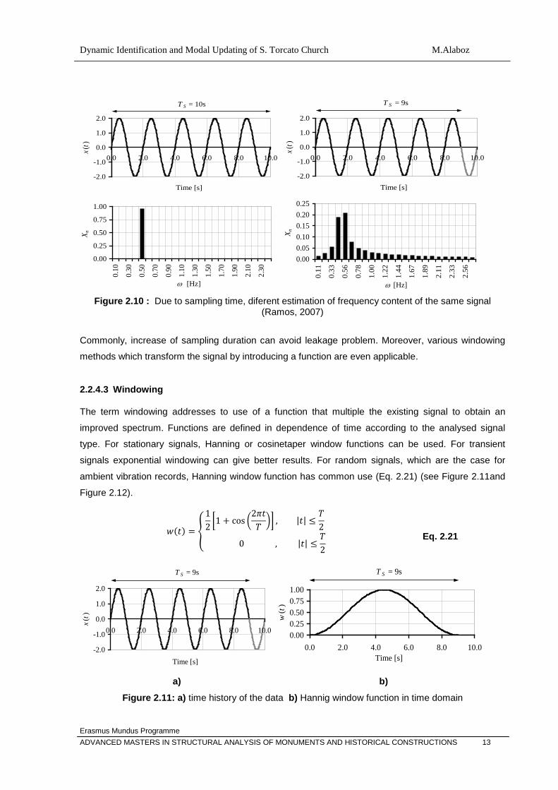
Figure 2.10 : Due to sampling time, diferent estimation of frequency content of the same signal
(Ramos, 2007) ....................................................................................................................................... 13
Figure 2.11: a) time history of the data b) Hannig window function in time domain ................... 13
Figure 2.12: a) Modified time history of the data b) Improved frequency response .................. 14
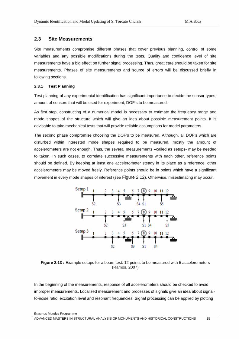
Figure 2.13 : Example setups for a beam test. 12 points to be measured with 5 accelerometers
(Ramos, 2007) ....................................................................................................................................... 15
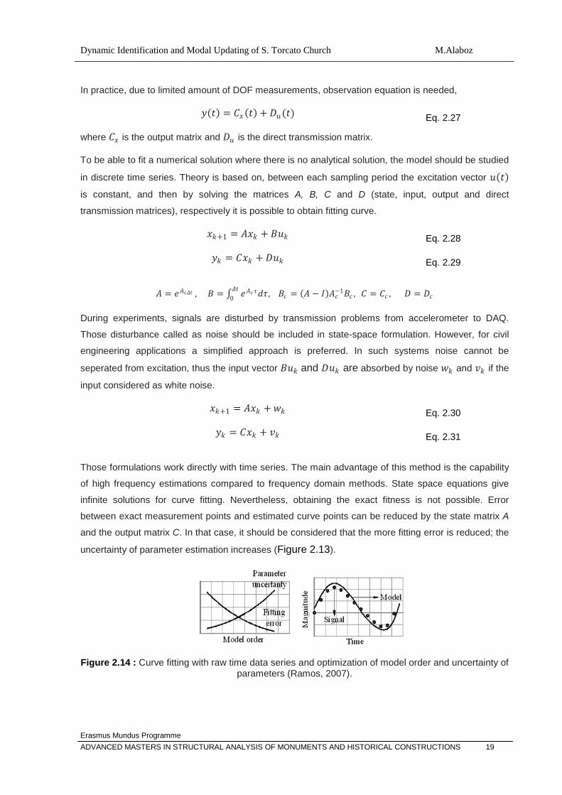
Figure 2.14 : Curve fitting with raw time data series and optimization of model order and uncertainty of
parameters (Ramos, 2007). .................................................................................................................. 19
Figure 3.1 : Early stages of construction, before the towers were constructed (San Torcato Museum)
............................................................................................................................................................... 20
Figure 3.2 : After complation of the north tower (San Torcato Museum) .............................................. 20
Figure 3.3 : Gound level plan (UMinho, Civil Engineering Dept.,1999) ................................................ 21
Figure 3.4 : Balcony of the church ......................................................................................................... 21
Figure 3.5 : Main nave and arch supported barrel vault ....................................................................... 22
Figure 3.6 : Timber roof and stone pillars that carry the roof ................................................................ 22
Figure 3.7 : Reinforced concrete cover of the apse vault and concrete walls ...................................... 23
Figure 3.8 : Crack pattern on main facade ............................................................................................ 24
Figure 3.9 : a) Crack on the floor of balcony and b) the crack on the facade wall ................................ 25
Figure 3.10 : Soil section according to investigation results ................................................................. 25
Figure 3.11 : Crack monitoring .............................................................................................................. 26
Figure 3.12 : Inclination measurements with tiltometer ......................................................................... 26
Figure 3.13 : Placement of accelerometers on towers and order of setups ......................................... 27
Figure 3.14 : Placement of accelerometers on balcony ........................................................................ 27
Figure 3.15 : Mode shapes of north tower ............................................................................................ 28
Figure 3.16 : Mode shapes of south tower (Ramos&Aguilar,2007) ...................................................... 28

M.Alaboz Dynamic Identification and Modal Updating of S. Torcato Church
Erasmus Mundus Programme xiv ADVANCED MASTERS IN STRUCTURAL ANALYSIS OF MONUMENTS AND HISTORICAL CONSTRUCTIONS
Figure 3.17 : Mode shapes of balcony (Ramos & Aguilar, 2007) .......................................................... 29
Figure 4.1 : a) Accelerometer used in test and b) DAQ system ............................................................ 30
Figure 4.2 : Data acquisition system set on the main nave ................................................................... 31
Figure 4.3 : Measured DOFs in towers. ................................................................................................. 32
Figure 4.4 : Measured DOFs in stair level and balcony ........................................................................ 32
Figure 4.5 : Plan of measured DOFs ..................................................................................................... 33
Figure 4.6 : Acceleration time graphs of Setup 1 – Setup 4 .................................................................. 35
Figure 4.7 : Acceleration time graphs of Setup 5 – Setup 8 .................................................................. 36
Figure 4.8 : Acceleration time graph of Setup 9 .................................................................................... 37
Figure 4.9 : Frequency decomposition graph of Setup 1 to Setup 4 ..................................................... 38
Figure 4.10 : Frequency decomposition graph of Setup 5 to Setup 8 ................................................... 39
Figure 4.11 : Frequency decomposition graph of Setup 9 .................................................................... 40
Figure 4.12 : Frequency decomposition of setups and picked peaks ................................................... 41
Figure 4.13 : EFDD graph of all setups and picked peaks .................................................................... 42
Figure 4.14 : CFDD frequency domain graph and picked peaks .......................................................... 42
Figure 4.15 : SSI method poles for setup1 imposed on frequency domain graph ................................ 43
Figure 4.16 : Mode shapes of SSI method frequency estimations ........................................................ 45
Figure 5.1 : a) CHX60 20 nodes brick element and b) CTP45 15 nodes wedge elements .................. 49
Figure 5.2 : CQ48I 16 nodes interface elements ................................................................................... 50
Figure 5.3 : 3d visualization of numerical model ................................................................................... 50
Figure 5.4 : Mode shapes presentation of numerical model ................................................................. 51
Figure 5.5 : Frequency versus scaled-MAC value comparison of Model 1 ........................................... 52
Figure 5.6 : Mode shape comparison of experimental and numerical models of Model 1 .................... 53
Figure 5.7 : Normalized modal displacement comparisons of numerical and experimental model ...... 55
Figure 5.8 : Crack definition of numerical model ................................................................................... 57
Figure 5.9 : Evaluation of modification by means of average frequency ratio and average MAC ........ 58
Figure 5.10 : Evaluation of modification by means of average frequency ratio and average MAC for
Mode 3 ................................................................................................................................................... 59
Figure 5.11 : Mode shape comparison of the model with crack definition ............................................ 60
Figure 5.12 : Interface elements with different properties ..................................................................... 61
Figure 5.13 : Mode shapes of Model 2 ................................................................................................. 62
Figure 5.14 : Effect of increasing the elastic properties of soill ............................................................. 63
Figure 5.15 : Experimental and numerical model comparison of the modified model .......................... 64
Figure 5.16 : Mode shapes comparison of the model with experimental model .................................. 65
Figure 5.17 : Interface elements defined at the edge of missing part ................................................... 66
Figure 5.18 : Effect of modification in frequency ratio and average MAC values of the model ............. 67
Figure 5.19 : Frequency versus MAC value presentation of modified model in Step 4 ........................ 68
Figure 5.20 : Mode shapes comparison of the model in Step 4 with the experimental model .............. 69

Dynamic Identification and Modal Updating of S. Torcato Church M.Alaboz
Erasmus Mundus Programme ADVANCED MASTERS IN STRUCTURAL ANALYSIS OF MONUMENTS AND HISTORICAL CONSTRUCTIONS xv
Figure 5.21 : Effect of modification in frequency ratio and average MAC values of the model ............ 70
Figure 5.22 : Frequency versus MAC value presentation of the modified model ................................. 72
Figure 5.23 : Mode shape comparison of the model in Step 2 with experimental model ..................... 73
Figure 5.24 : Frequency versus MAC value presentation of the model modified with Douglas-Reid
method ................................................................................................................................................... 76
Figure 5.25 : Mode shapes comparison of the modified model ........................................................... 77
Figure 5.26 : Normalized Modal displacement comparison of each DOF for mode shapes ................. 79
Figure 5.27 : Effect of crack definition in frequency error versus average MAC ................................... 80
Figure 5.28 : Initial model without modifications and the effect of each modification step ................... 81

M.Alaboz Dynamic Identification and Modal Updating of S. Torcato Church
Erasmus Mundus Programme xvi ADVANCED MASTERS IN STRUCTURAL ANALYSIS OF MONUMENTS AND HISTORICAL CONSTRUCTIONS

Dynamic Identification and Modal Updating of S. Torcato Church M.Alaboz
Erasmus Mundus Programme ADVANCED MASTERS IN STRUCTURAL ANALYSIS OF MONUMENTS AND HISTORICAL CONSTRUCTIONS xvii
LIST OF TABLES
Table 3.1 : Frequency and damping estimation of north tower (Ramos & Aguilar,2007) ...... 28
Table 3.2 : Frequency and damping estimation of south tower (Ramos & Aguilar, 2007) ..... 28
Table 3.3 : Frequency and damping estimation of facade (Ramos & Aguilar, 2007) ............ 29
Table 4.1 : The chart that shows the measured DOF’s with their direction in each setup ..... 33
Table 4.2 : Peak acceleration of setups and average RMS values ....................................... 37
Table 4.3 : Frequency estimation of setups by FDD method ................................................ 40
Table 4.4 : Frequency estimation of all setups ..................................................................... 41
Table 4.5 : EFDD method frequency and damping estimations for all setups and their
standard variation ................................................................................................................ 42
Table 4.6 : CFDD method frequency and damping estimations for all setups and their
standard deviation ............................................................................................................... 43
Table 4.7 : SSI-PC method frequency and damping estimations for all setups .................... 43
Table 4.8 : Frequency estimations of different identification methods [Hz] ........................... 44
Table 4.9 : Frequency error of different methods based on SSI values ................................ 44
Table 4.10 : Damping estimation and standard variation of different methods ..................... 44
Table 5.1 : Material properties of masonry ........................................................................... 50
Table 5.2 : Natural frequencies of the model with rigid foundations ...................................... 51
Table 5.3 : Frequency and MAC value comparison of Model 1 ............................................ 52
Table 5.4 : Modified models and frequency comparison ...................................................... 56
Table 5.5 : Frequency and MAC comparison of the modified model .................................... 56
Table 5.6 : Elastic properties of cracked region .................................................................... 58
Table 5.7 : Frequency and MAC values of modified models ................................................. 58
Table 5.8 : Comparison of MAC values before and after crack definition ............................. 59
Table 5.9 : Soil properties of the model with elastic foundation ............................................ 61
Table 5.10 : Modal analysis frequency estimations and MAC comparison with experimental
model ................................................................................................................................... 62
Table 5.11 : Modification parameters of soil properties ........................................................ 63
Table 5.12 : Frequency and MAC value comparison of modified models ............................. 63
Table 5.13 : Frequency and mode shape comparison of modified model with experimental
model ................................................................................................................................... 64
Table 5.14 : Contribution of modification in MAC for the model ............................................ 64
Table 5.15 : Modification parameters of interface elements ................................................. 66
Table 5.16 : Frequency and MAC value of each modified model ......................................... 67

M.Alaboz Dynamic Identification and Modal Updating of S. Torcato Church
Erasmus Mundus Programme xviii ADVANCED MASTERS IN STRUCTURAL ANALYSIS OF MONUMENTS AND HISTORICAL CONSTRUCTIONS
Table 5.17 : Frequency and mode shape comparison of modified model with experimental
model ................................................................................................................................... 67
Table 5.18 : Contribution of modifications in MAC values for the model ............................... 68
Table 5.19 : Modification parameters of interface elements ................................................ 70
Table 5.20 : Frequency and MAC value of each modified model .......................................... 71
Table 5.21 : Frequency and mode shape comparison of modified model with experimental
model ................................................................................................................................... 71
Table 5.22 : MAC value contribution of modifications for the model in Step 2 ...................... 71
Table 5.23 : Initial Properties of the modified model before optimization .............................. 74
Table 5.24 : Upper and lower bound properties variables .................................................... 74
Table 5.25 : Frequencies of the models for each variable [Hz] ............................................. 75
Table 5.26 : Non linear estimation of optimum modification parameters ............................... 75
Table 5.27 : Comparison of the model modified with Douglas-Reid ..................................... 75
Table 5.28 : Frequency and MAC value comparison of the modified model ......................... 76
Table 5.29 : Modification parameters of cracked region ....................................................... 80
Table 5.30 : NMD values of the modified model ................................................................... 80

Dynamic Identification and Modal Updating of S. Torcato Church M.Alaboz
Erasmus Mundus Programme ADVANCED MASTERS IN STRUCTURAL ANALYSIS OF MONUMENTS AND HISTORICAL CONSTRUCTIONS xix


Dynamic Identification and Modal Updating of S. Torcato Church M.Alaboz
Erasmus Mundus Programme ADVANCED MASTERS IN STRUCTURAL ANALYSIS OF MONUMENTS AND HISTORICAL CONSTRUCTIONS 1
1. INTRODUCTION
Historical structures which are the part of cultural heritage take their place in the modern world by
representing the past experiences, technical and aesthetical approaches. Besides being far from our
technical knowledge and understanding, many of them achieved to be stand till our times with their
practical solutions for structural problems.
However the abrasive effect of time causes various damages or deficiencies on structures; from
natural events to human based damages. In order to maintain their existence for the following
generations, those sources of damages should be avoided and any needed intervention should be
taken according to the modern conservation approaches.
Nevertheless, before any intervention to a structure, identification of all structural properties and
damage sources has a significant importance. Although numerical model analyses methods allow one
to simulate various cases, estimation or assumptions of structural properties are not easy. To alter
these difficulties many non-destructive methods have being developed but the information of those
techniques rather local or insufficient.
Experimental dynamic identification techniques, which are based on the acceleration records of a
structure, allow us to obtain natural frequencies, mode shapes and damping coefficients of a structure.
These data represent the overall dynamic capacity of a structure as a result of its physical properties
that are unknown or difficult to obtain. By this way, real response of the structure under specified or
unknown excitations can be used to modify structural models with the help of any test results that
represent only local properties.
1.1 Objectives
The aim of this dissertation is to carry out a modal identification analysis of S. Torcato Church and to
tune a finite element model for further numerical analyses. The work includes the field work for
experimental estimation of the modal parameters (natural frequencies, mode shapes and damping
coefficients) with dynamic test equipments.
Estimated dynamic properties of the structure were used to tune a previous finite element model.
Evaluation of the numerical model and the selection of updating parameters is part of the present
study. Underlining the deficiencies and improving the efficiency of the numerical model is the main
target of the study.

M.Alaboz Dynamic Identification and Modal Updating of S. Torcato Church
Erasmus Mundus Programme 2 ADVANCED MASTERS IN STRUCTURAL ANALYSIS OF MONUMENTS AND HISTORICAL CONSTRUCTIONS
1.2 Out Line
This thesis study consists of six chapters. The introduction, Chapter 1 gives general information about
the outline of the study, concepts of dynamic experiments and modal updating methods. The
objectives are also discussed.
Chapter 2 aims to give brief information about the basis of dynamics and experimental dynamic tests.
In the first section of the chapter, basic dynamic terms and fundamental dynamic problems are
explained on single and multi degree of freedoms systems. In the following sections, theory of
experimental analysis, the equipments, common problems and dynamic identification methods are
explained.
Chapter 3 introduces the San Torcato Church with its historical, architectural and structural properties
and states the actual condition of the structure. In this chapter damages in the light of previous
investigations are highlighted to constitute a base for further chapters.
Chapter 4 gives information about the field work for experimental dynamic identification. Test planning
procedure is given with details. Preliminary analysis of setups, comparison of different identification
methods and estimation of dynamic properties are included.
In Chapter 5, modal updating theory and tools for comparisons are discussed as an introduction.
Following sections have the explanation of numerical model and its properties. Effects of parametric
modifications are discussed and modal updating is performed by using robust modification algorithms.
Chapter 6 contains the conclusions. As a summary of the study, difficulties faced during the work,
discussion of results and recommendations for further studies are stated.

Dynamic Identification and Modal Updating of S. Torcato Church M.Alaboz
Erasmus Mundus Programme ADVANCED MASTERS IN STRUCTURAL ANALYSIS OF MONUMENTS AND HISTORICAL CONSTRUCTIONS 3
2 EXPERIMENTAL DYNAMIC IDENTIFICATION TECHNIQUES
2.1 Basic Dynamics
Structural dynamic analysis methods aim to identify the stress and response of the structure under
arbitrary dynamic loadings. Dynamics of any system could be defined as time-varying, as the direction,
magnitude and position of the loads vary with time.
Response of any system can be defined as deterministic or nondeterministic. If the time variation of
dynamic forces acting on the system is fully known, then the system is defined as deterministic. In
case of the loading is arbitrary, which is the real case for most of the time, and then the time variation
can be defined with statistical approaches (Clough, 1995).
Within the following parts, dynamic properties of systems and basic source of dynamic theory will be
briefly discussed.
2.1.1 Single Degree of Freedom Systems
Any mechanical or structural systems which are exposed to external source of excitations or dynamic
loadings, give response to the loads with their initial resistive properties. Those properties are defined
as mass, stiffness and energy dissipation capability, damping.
Although many engineering structures have multi degree of freedom (DOF), definition of dynamic
behaviour of a single degree of freedom system is useful to understand the multi degree of freedom
systems. Dynamic terms can be explained by using a typical demonstration of a concentrated mass
on a massless column (Figure 2.1).
Figure 2.1 SDOF structure
The system is defined by a mass on top connected to ground by a column that has specified stiffness
that contracts with the movements of the mass. Any force act on the mass m cause displacement
proportional to the stiffness of the system k. When the forces replaced, the system starts to oscillate in
a specific frequency. In damped structures, by the time passes the velocity of the cycles decreases
until the initial position of the mass is satisfied. In damped systems, energy is dissipated in different

M.Alaboz Dynamic Identification and Modal Updating of S. Torcato Church
Erasmus Mundus Programme 4 ADVANCED MASTERS IN STRUCTURAL ANALYSIS OF MONUMENTS AND HISTORICAL CONSTRUCTIONS
mechanisms such transformation of kinetic energy to thermal energy, formation of cracks or friction
between structural or non-structural elements (Chopra, 2001).
Total resistance of the system under excitations consists of stiffness k that is proportional to the
magnitude of the displacement, energy dissipation factor that is proportional to the velocity of the
displacement and inertia of the mass proportional to the acceleration of the displacement. Thus, the
equilibrium of all the forces gives the equation of motion (Eq. 2.1).
𝒎𝒎�̈�𝒖 + 𝒄𝒄�̇�𝒖 + 𝒌𝒌𝒖𝒖 = 𝒑𝒑(𝒕𝒕) Eq. 2.1
where m is mass, c is damping, k stiffness, u is displacement and p(t) is the acting force on the system
depending on time.
Equation of motion can be solved with four different methods. One is called the classical method that
allows analytical solution, Duhamel’s Integral in the case of arbitrary impulse, Laplace or Fourier
Transform methods to obtain the response in frequency domain or with numerical methods such as
Newmar Method.
Analytical solution can be derived from free vibration theory. If the system is disturbed from its static
equilibrium position by imparting the mass some displacement and release, the acting force is then
equal to zero. When the system released, in damping free systems, it oscillates in a specific frequency
(Figure 2.2). The equation of motion (Eq. 2.2) can be solved by (Eq. 2.3)
𝒎𝒎�̈�𝒖 + 𝒌𝒌𝒖𝒖 = 𝟎𝟎 Eq. 2.2
𝑢𝑢(𝑡𝑡) = 𝐴𝐴𝐴𝐴𝐴𝐴𝐴𝐴𝜔𝜔𝑛𝑛𝑡𝑡 + 𝐵𝐵𝐴𝐴𝐵𝐵𝑛𝑛𝜔𝜔𝑛𝑛𝑡𝑡 Eq. 2.3
Then 𝑤𝑤𝑛𝑛 is obtained, it gives the natural circular frequency of the system in rad/s.
𝑤𝑤𝑛𝑛 = �𝑘𝑘𝑚𝑚
[rad/s] Eq. 2.4
Linear natural frequency 𝑓𝑓𝑛𝑛 and period 𝑇𝑇 can be derived easily (Eq. 2.5) , as ;
a) 𝑓𝑓𝑛𝑛 = 1𝑇𝑇
= 𝑤𝑤𝑛𝑛2𝜋𝜋
[Hz] , b) 𝑇𝑇 = 2𝜋𝜋𝑤𝑤𝑛𝑛
[sec] Eq. 2.5

Dynamic Identification and Modal Updating of S. Torcato Church M.Alaboz
Erasmus Mundus Programme ADVANCED MASTERS IN STRUCTURAL ANALYSIS OF MONUMENTS AND HISTORICAL CONSTRUCTIONS 5
Figure 2.2 : Response history graph of a free vibration system (Chopra, 2001)
When damping comes to picture as in all real cases, by differentiating the equation of motion (Eq.
2.6), it is possible obtain;
𝑚𝑚�̈�𝑢 + 𝐴𝐴�̇�𝑢 + 𝑘𝑘𝑢𝑢 = 0 Eq. 2.6
𝑢𝑢 = 𝑒𝑒−𝜉𝜉𝑤𝑤𝑛𝑛 𝑡𝑡 �𝑢𝑢0 cos𝜔𝜔𝐷𝐷𝑡𝑡 +𝑢𝑢0̇ + 𝑢𝑢0𝜉𝜉𝜔𝜔𝑛𝑛
𝜔𝜔𝐷𝐷sin𝜔𝜔𝐷𝐷𝑡𝑡�
Eq. 2.7
Where 𝜉𝜉 is damping ratio and 𝜔𝜔𝐷𝐷 damped frequency given by;
𝜉𝜉 = 𝐶𝐶
𝐶𝐶𝐴𝐴𝑐𝑐 Eq. 2.8
and;
𝜔𝜔𝐷𝐷 = 𝜔𝜔𝑛𝑛�1 − 𝜉𝜉2
Eq. 2.9
When an arbitrary impulse p(t) acts on the system, then by solving the second order differential
equation Duhamel’s integral, the response is derived as;
𝑞𝑞(𝑡𝑡) = 1
𝑚𝑚𝜔𝜔𝐷𝐷∫ 𝑝𝑝(𝜏𝜏)𝑒𝑒−𝜉𝜉𝜔𝜔𝑛𝑛 (𝑡𝑡−𝜏𝜏) sin[𝜔𝜔𝐷𝐷(𝑡𝑡 − 𝜏𝜏)]𝑑𝑑𝜏𝜏𝑡𝑡
0 , 𝑡𝑡 > 𝜏𝜏
Eq. 2.10
where 𝜏𝜏 is the reference instant. Another way of calculating the response of a system can be realized in frequency domain by means of
Fourier Transformation. Definition of Fourier Transformation 𝑋𝑋 for function 𝑥𝑥(𝑡𝑡) is;

M.Alaboz Dynamic Identification and Modal Updating of S. Torcato Church
Erasmus Mundus Programme 6 ADVANCED MASTERS IN STRUCTURAL ANALYSIS OF MONUMENTS AND HISTORICAL CONSTRUCTIONS
𝑋𝑋(𝜔𝜔) = � 𝑥𝑥(𝑡𝑡)𝑒𝑒−𝑗𝑗𝜔𝜔𝑡𝑡+∞
−∞
Eq. 2.11
If the Fourier Transformation is applied in both sides of equation of motion, then it reads;
−𝑚𝑚𝜔𝜔2𝑄𝑄(𝜔𝜔) + 𝐴𝐴𝑗𝑗𝜔𝜔𝑄𝑄(𝜔𝜔) + 𝑘𝑘𝑄𝑄(𝜔𝜔) = 𝑃𝑃(𝜔𝜔) Eq. 2.12
Solving the equation with respect to 𝑄𝑄(𝜔𝜔), it is seen that the response of the structure is proportional
the complex function 𝐻𝐻(𝜔𝜔), so called Frequency Response Function (FRF).
𝑄𝑄(𝜔𝜔) =𝑃𝑃(𝑤𝑤)
−𝑚𝑚𝜔𝜔2 + 𝐴𝐴𝑗𝑗𝜔𝜔 + 𝑘𝑘= 𝐻𝐻(𝜔𝜔)𝑃𝑃(𝜔𝜔)
Eq. 2.13
The main advantage of frequency domain is to allow evaluation of the response in correlation with the
excitation. This constitutes the bases of seismic analysis and experimental dynamic identification
theories as well.
2.1.2 Multi Degree of Freedom Systems
As it was discussed previously, many times multi degree of freedom systems can be solved like single
degree freedom systems by means of simplifications. Like in the given example (Figure 2.3), total
mass of one floor is lumped in a concentrated mass point and possible movements of the point (DOF)
described in one direction where in reality rotation and longitudinal transformation of the point is
possible.
Figure 2.3 : Definition of the system in equilibrium and its components (Chopra, 2001).
However, m degree of freedom systems can be solved with equation of motion.
𝑀𝑀�̈�𝑞(𝑡𝑡) + 𝐶𝐶2�̇�𝑞(𝑡𝑡) + 𝐾𝐾𝑞𝑞(𝑡𝑡) = 𝑝𝑝(𝑡𝑡) Eq. 2.14
In that equation M, C2 and K represent the nxn matrices of mass, damping and stiffness. For the
solution of the equation, Fourier transformation can be used. However, the solution of the problem

Dynamic Identification and Modal Updating of S. Torcato Church M.Alaboz
Erasmus Mundus Programme ADVANCED MASTERS IN STRUCTURAL ANALYSIS OF MONUMENTS AND HISTORICAL CONSTRUCTIONS 7
requires inverse of complex matrix nxn for each frequency. Instead, modal approach is preferred
which is based on eigenvalue solution. When damping is neglected, the solution is given by,
𝑞𝑞(𝑡𝑡) = 𝜑𝜑𝐵𝐵𝑒𝑒𝜆𝜆𝐵𝐵𝑡𝑡 Eq. 2.15
where 𝜑𝜑𝐵𝐵 are the real eigenvectors (i=1,...,m) and 𝜆𝜆𝐵𝐵
2 are the eigenvalues. For free vibration systems,
the equation reads by substituting 𝑞𝑞(𝑡𝑡),
[𝐾𝐾 − (−𝜆𝜆2)𝑀𝑀]𝜑𝜑𝐵𝐵 = 0 V 𝐾𝐾ф = 𝑀𝑀ф𝛬𝛬
Eq. 2.16
Orthogonality properties of modal shape matrix allow normalizing matrices;
ф𝑚𝑚𝑇𝑇 𝑀𝑀ф𝑚𝑚 = 𝐼𝐼 ф𝑚𝑚𝑇𝑇 𝐾𝐾ф𝑚𝑚 = 𝛬𝛬2
Eq. 2.17
By adding damping properties and coordinate transformation, then equation of motion becomes;
𝐼𝐼𝑞𝑞�̈�𝑚 (𝑡𝑡) + 𝛤𝛤𝑞𝑞�̇�𝑚 (𝑡𝑡) + 𝛬𝛬2𝑞𝑞𝑚𝑚(𝑡𝑡) = �
⋱
1𝑚𝑚𝐵𝐵
⋱
�ф𝑇𝑇𝑝𝑝(𝑡𝑡)
Eq. 2.18
where 𝐼𝐼 is modal mass, 𝛤𝛤 is modal damping and 𝛬𝛬2 is modal stiffness. After the equation is obtained in similar form of single degree of freedom system, Fourier
transformation can be used. Diagonal terms of FRF can be formed as given;
𝐻𝐻(𝐵𝐵,𝑘𝑘)(𝜔𝜔) = ∑ ф𝐵𝐵,𝑗𝑗 ф𝑘𝑘 ,𝑗𝑗
�𝜔𝜔𝑛𝑛2−𝜔𝜔2�+𝐵𝐵(2𝜉𝜉𝑛𝑛𝜔𝜔𝑛𝑛𝜔𝜔)
,𝑛𝑛𝑗𝑗=1 i Λ k=1,....,m
Eq. 2.19
2.2 Experimental Modal Analysis
Considering the modern conservation criteria that demands minimum intervention and preservation of
construction techniques, understanding of any damage phenomena or evaluation of seismic
vulnerability have significant importance. For this purpose identification of a structure or mathematic
model must represent the existing properties and conditions. Concerning that point, different non-
destructive inspection techniques are being used that provide local information for the estimation of
global properties. However, seismic behaviour of a structure or any possible earthquake damage
occurrence is depended on global dynamic properties.
Dynamic behaviour of structures is defined by the mechanical properties of the materials, geometry of
the structure and its energy dissipation capabilities. When those variables are known, seismic
response of a structure can be analyzed for different earthquake excitations. These variables are
controllable in design processes with many safety coefficients. For the analysis of historical structures

M.Alaboz Dynamic Identification and Modal Updating of S. Torcato Church
Erasmus Mundus Programme 8 ADVANCED MASTERS IN STRUCTURAL ANALYSIS OF MONUMENTS AND HISTORICAL CONSTRUCTIONS
to evaluate their safety, those variables are difficult to estimate even with the help of destructive or
non-destructive structural tests.
Experimental dynamic identification techniques, which are mainly based on the acceleration records of
a structure, allow us to obtain natural frequencies, mode shapes and damping coefficients. These data
represent the overall respond of a structure as a result of its physical properties that are unknown or
difficult to obtain. By this way, real response of the structure can be used to optimize any test results
that represent only local properties and to modify structural models.
Modal testing is mostly based on the observation of the response of a structure under any excitation.
Response of the structure is generally observed in frequency domain while the recorded measure can
vary as acceleration, velocity or displacement. In order to obtain frequency response function as a
target, various equipments has to be used properly due to excitation source or measured physical
outcome.
If the excitation source is wanted to be measured, a controlled excitation mechanism is needed.
Moreover, to be able to capture the response of the structure in any physical measure, special
equipments mostly called as sensor or transducer should be used. For the processes of collected
data, a digital converter, signal conditioning and as final signal processing software is needed. The
whole process is called as data acquisition. Component of the any data acquisition system (DAQ) can
be sorted as given in Figure 2.4.
Figure 2.4 : Data acquisition system body and its components
2.2.1 Excitation Mechanisms
Excitation mechanisms are preferred when the response of the structure is not sufficient under
ambient vibrations. In that case, controlled excitation mechanisms can be used. Most frequently used
excitation mechanisms are, shakers, drop weight systems and impact hammers.
Shakers allow user to control both the frequency and force. However, their use demands to stop the
function of the structure during the experiment. Also, the setting of the system is rather expensive and
time taking.
While the shakers are used for big scale structures like bridges and dams, impact hammers can give
sufficient results for light weight structures. With impact hammer, it is possible to excite the structure
Data Acquisition
Excitation Sensing Data Transmission
Analog to Digital
ConversionData
StorageData
Filtering

Dynamic Identification and Modal Updating of S. Torcato Church M.Alaboz
Erasmus Mundus Programme ADVANCED MASTERS IN STRUCTURAL ANALYSIS OF MONUMENTS AND HISTORICAL CONSTRUCTIONS 9
with different spectral impact energy, by changing the weight of the head, velocity of impact and by
changing the tips with different toughness (see Figure 2.5) (Ramos, 2007).
a) b)
Figure 2.5 : a) Drop weight system and b) impact hammer
Weight drop systems are advantageous with the possibility of controlling the frequency content of the
impact, changing the damping properties and higher energy apply to the structure compared with
impact hammer test (Figure 2.5) (Ramos, 2007).
2.2.2 Sensors
For the purpose of dynamic system identification, movement of the structure has to be captured in
discrete time. Movement of any system can be derived from acceleration or velocity as well as the
measurement of displacement either. However, due to practical limitations, mostly acceleration
measurements are preferred for dynamic identification and monitoring systems.
When choosing the accelerometers for an experiment, variables listed below should be considered;
• Types of data to be acquired
• Sensor types, number and locations
• Bandwidth, sensitivity (dynamic range)
• Data acquisition/transmittal/storage system
• Power requirements (energy harvesting)
• Sampling intervals
• Processor/memory requirements
• Excitation source (active sensing)

M.Alaboz Dynamic Identification and Modal Updating of S. Torcato Church
Erasmus Mundus Programme 10 ADVANCED MASTERS IN STRUCTURAL ANALYSIS OF MONUMENTS AND HISTORICAL CONSTRUCTIONS
As stated above, due to high frequency content of the structures, acceleration measurements
preferred rather than velocity or displacement measurements. Moreover, need of using a base point
as a reference for displacement measurements, makes the displacement based measurements almost
impossible (Ramos, 2007).
2.2.2.1 Piezoelectric Accelerometer
Piezoelectric accelerometer is composed of a spring-mass-damper system and produces signals
proportional to the acceleration of the mass in a frequency band below its resonant frequency (Figure
2.6). Those kinds of accelerometers require conditioning before starting to record.
Piezoelectric transducers are advantageous with their size, not using external power source, having a
good signal to noise ratio and linear in a wide frequency range. However, except some types, most of
the piezoelectric accelerometers are not able to capture low frequencies close to zero –like in very
flexible structures- (Ramos, 2007).
Figure 2.6 : Piezoelectric Accelerometer (Ramos, 2007)
2.2.2.2 Piezoresistive Accelerometer
Piezoresistive accelerometers consist of a plate which is hold by springs (Figure 2.7). The main
advantage of the type is to capture uniform signals which cannot be captured by piezoelectric
accelerometers. Their disadvantages are cited as requirement of external power supply, bigger size
and limited band width with maximum 1000 Hz.
Housing
Fixed platesDiaphragm(free ends)
Applied acceleration
Lead wire
Electrical connector
Electronics
Figure 2.7 : Piezoresistive accelerometer (Ramos, 2007).
HousingSeismic mass
ElectrodePiezoelectric material
Applied acceleration
Lead wire
Electrical connector
+−

Dynamic Identification and Modal Updating of S. Torcato Church M.Alaboz
Erasmus Mundus Programme ADVANCED MASTERS IN STRUCTURAL ANALYSIS OF MONUMENTS AND HISTORICAL CONSTRUCTIONS 11
2.2.2.3 Piezoresistive Accelerometer
Force balance accelerometers are passive accelerometers likewise capacitive accelerometers and
produce signals proportional to the mass which is fixed through four suspension beams. The mass is
located between two capacitive plates and when it moves, plates force the mass to back to the initial
position (Figure 2.8). Acceleration is obtained by the differential voltage required for the force.
Force-balance transducers are high sensitive and rugged. Dynamic range of the accelerometers can
be configured to a dynamic range equal to ±0.5, ±1, ±2 and ±4 g and frequency range from DC to 100
Hz with a maximum resolution of 1 μg (Ramos, 2007).
Figure 2.8 : Force balance accelerometer (Ramos, 2007)
2.2.3 Data Acquisition Device
Data acquisition devices can be defined as a device which converts the analogue data to digital data
in discrete-time intervals. Sometimes signal conditioning is needed before processing the data. Most
common problems can be stated as follows:
• Low excitation level of recorded data. It has to be amplified in order to increase the resolution
and reduce noise. High accuracy could be obtained by configuring the data acquisition system
where the maximum voltage range of the conditioned signal equals to the maximum input
range of the Analogue Digital Converter(ADC).
• Signals are transferred with high voltage. Thus, transition should be isolated from voltage
changes like ground potentials or any voltage sources.
• Undesired signals which may contain high frequencies should be filtered. For this case anti-
aliasing filters remove all frequency components that are higher than the input bandwidth.
• If the transducer type is passive, DAQ provides the external voltage.
• DAQ system is responsible of linearization of any nonlinear transducer response during the
measurements.
Moving capacitor plate
Central plate
Fixed outercapacitor plates
Anchors
Suspensionbeams
Unit cell
Applied accelerationCentral plate
Anchors
Unit cell

M.Alaboz Dynamic Identification and Modal Updating of S. Torcato Church
Erasmus Mundus Programme 12 ADVANCED MASTERS IN STRUCTURAL ANALYSIS OF MONUMENTS AND HISTORICAL CONSTRUCTIONS
2.2.4 Common Signal Conditioning Functions
2.2.4.1 Aliasing
Due to the fact that the acceleration measurements are taken in discrete time, sampling rate has a
significant importance to be able to capture desired frequencies. In case of using lower sampling rate
then real frequency, the signal prediction will come up with a different lower frequency content which
can fit with the measured points (Figure 2.9).
Figure 2.9 : Time-Acceleration graph of the same signal measured with different sampling rates (Ramos, 2007)
To avoid aliasing problem, low pass filter must used with the nyquist frequency. Nyquist frequency
should be taken as twice or slightly higher than the maximum expected frequency of interest (Eq.
2.20). However, the ADC system itself has a limited resolution when the analogue data is being
transformed to digital data.
𝑓𝑓𝐴𝐴 = 1∆𝑓𝑓≥ 2 × 𝑓𝑓𝑁𝑁𝑁𝑁𝑞𝑞 𝑓𝑓𝐴𝐴 ≥ 2 × 𝑓𝑓𝑚𝑚𝑚𝑚𝑥𝑥 Eq. 2.20
2.2.4.2 Leakage
While it is possible to define a periodic signal through infinite time series, experimental measurement
are recorded in discrete time series. Discrete Fourier Transform series can be easily obtained by Fast
Fourier Transformations. However, transformation of infinite series into frequency domain brings the
problem leakage if the measure time is not an integer multiple of the signal period. If the sampling
duration is not an integer of desired period, the signal can be interpreted as a composition of different
frequency contents (Figure 2.10).
-1.0
-0.5
0.0
0.5
1.0
0.0 2.0 4.0 6.0 8.0 10.0
Time [s]
Sign
al [m
g]
Continuous Signal Measured Signal
-1.0
-0.5
0.0
0.5
1.0
0.0 2.0 4.0 6.0 8.0 10.0
Time [s]
Sign
al [m
g]
Continuous Signal Measured Signal
Dynamic Identification and Modal Updating of S. Torcato Church M.Alaboz
Erasmus Mundus Programme ADVANCED MASTERS IN STRUCTURAL ANALYSIS OF MONUMENTS AND HISTORICAL CONSTRUCTIONS 13
Figure 2.10 : Due to sampling time, diferent estimation of frequency content of the same signal
(Ramos, 2007)
Commonly, increase of sampling duration can avoid leakage problem. Moreover, various windowing
methods which transform the signal by introducing a function are even applicable.
2.2.4.3 Windowing
The term windowing addresses to use of a function that multiple the existing signal to obtain an
improved spectrum. Functions are defined in dependence of time according to the analysed signal
type. For stationary signals, Hanning or cosinetaper window functions can be used. For transient
signals exponential windowing can give better results. For random signals, which are the case for
ambient vibration records, Hanning window function has common use (Eq. 2.21) (see Figure 2.11and
Figure 2.12).
𝑤𝑤(𝑡𝑡) = �
12�1 + cos �
2𝜋𝜋𝑡𝑡𝑇𝑇�� , |𝑡𝑡| ≤
𝑇𝑇2
0 , |𝑡𝑡| ≤𝑇𝑇2
�
Eq. 2.21
a) b)
Figure 2.11: a) time history of the data b) Hannig window function in time domain
-2.0
-1.0
0.0
1.0
2.0
0.0 2.0 4.0 6.0 8.0 10.0
Time [s]
x(t)
T S = 10s
-2.0
-1.0
0.0
1.0
2.0
0.0 2.0 4.0 6.0 8.0 10.0
Time [s]
x(t)
T S = 9s
0.00
0.25
0.50
0.75
1.00
0.10
0.30
0.50
0.70
0.90
1.10
1.30
1.50
1.70
1.90
2.10
2.30
ω [Hz]
X n
0.000.050.100.150.200.25
0.11
0.33
0.56
0.78
1.00
1.22
1.44
1.67
1.89
2.11
2.33
2.56
ω [Hz]X n
-2.0
-1.0
0.0
1.0
2.0
0.0 2.0 4.0 6.0 8.0 10.0
Time [s]
x(t)
T S = 9s
0.000.250.500.751.00
0.0 2.0 4.0 6.0 8.0 10.0Time [s]
w(t
)
T S = 9s

M.Alaboz Dynamic Identification and Modal Updating of S. Torcato Church
Erasmus Mundus Programme 14 ADVANCED MASTERS IN STRUCTURAL ANALYSIS OF MONUMENTS AND HISTORICAL CONSTRUCTIONS
a) b)
Figure 2.12: a) Modified time history of the data b) Improved frequency response
2.2.4.4 Filters
Similar to windowing functions which are applicable on time domain data, filter functions modify the
spectrum signals. According to the aim, different types of filters can be used such as low-pass, high-
pass and band-limited filters which they filter the frequencies in processed data.
2.2.4.5 Decimation
Decimation is the processes of reducing the number of records without loose of information. It is
based on skipping one point to the other by keeping the signal curve constant. By this way while the
frequency content keeps constant, the processing of the records speeds up. To avoid aliasing
problem, it is advised to apply a low-pass filter with a frequency cut-off about 40% of the new sample
frequency.
2.2.4.6 Welch Method
Welch method is preferred for randomly excited systems. Methods based on averaging the FFT
transformations so that a smooth curve can be obtained. Nevertheless, the time segments used for
the method cause decrement of resolution when FFT applied. To alter this problem, time segments
overlapped with 2/3 or 1/2 ratios associated with the use of Hanning window.
-2.00
-1.00
0.00
1.00
2.00
0.0 2.0 4.0 6.0 8.0 10.0
Time [s]
x(t
)w(t
)
T S = 9s
0.00
0.05
0.10
0.15
0.20
0.11
0.33
0.56
0.78
1.00
1.22
1.44
1.67
1.89
2.11
2.33
2.56
ω [Hz]
Xn
Dynamic Identification and Modal Updating of S. Torcato Church M.Alaboz
Erasmus Mundus Programme ADVANCED MASTERS IN STRUCTURAL ANALYSIS OF MONUMENTS AND HISTORICAL CONSTRUCTIONS 15
2.3 Site Measurements
Site measurements compromise different phases that cover previous planning, control of some
variables and any possible modifications during the tests. Quality and confidence level of site
measurements have a big effect on further signal processing. Thus, great care should be taken for site
measurements. Phases of site measurements and source of errors will be discussed briefly in
following sections.
2.3.1 Test Planning
Test planning of any experimental identification has significant importance to decide the sensor types,
amount of sensors that will be used for experiment, DOF’s to be measured.
As first step, constructing of a numerical model is necessary to estimate the frequency range and
mode shapes of the structure which will give an idea about possible measurement points. It is
advisable to take mechanical tests that will provide reliable assumptions for model parameters.
The second phase compromise choosing the DOF’s to be measured. Although, all DOF’s which are
disturbed within interested mode shapes required to be measured, mostly the amount of
accelerometers are not enough. Thus, the several measurements –called as setups- may be needed
to taken. In such cases, to correlate successive measurements with each other, reference points
should be defined. By keeping at least one accelerometer steady in its place as a reference, other
accelerometers may be moved freely. Reference points should be in points which have a significant
movement in every mode shapes of interest (see Figure 2.12). Otherwise, misestimating may occur.
Figure 2.13 : Example setups for a beam test. 12 points to be measured with 5 accelerometers (Ramos, 2007)
In the beginning of the measurements, response of all accelerometers should be checked to avoid
improper measurements. Localized measurement and processes of signals give an idea about signal-
to-noise ratio, excitation level and resonant frequencies. Signal processing can be applied by plotting

M.Alaboz Dynamic Identification and Modal Updating of S. Torcato Church
Erasmus Mundus Programme 16 ADVANCED MASTERS IN STRUCTURAL ANALYSIS OF MONUMENTS AND HISTORICAL CONSTRUCTIONS
the power spectra of measured points. Primary measurements can be taken on reference points which
will be base for all setups. In case of low excitation or having locally low/extraordinary high responses,
reference points or any DOF can be changed during the test. Depending on the responses, change of
transducer types or even the use of external excitation sources can be needed.
After setting the system, other important issue is to decide sampling rate and sampling duration of
measurements. Sampling rate of measurements, affect estimation of frequencies. Sampling frequency
rate decision is based on Nquist frequency theorem which is defined as two times higher of the
expected frequency. In order to capture a frequency, the sampling rate should be at least equal to
Nyquist frequency.
Sampling duration is another important variable in experimental identification. Large number of points
should be recorded to have good resolution. In literature some different empirical approach can be
found. According to Rodrigues (Rodrigues,2001), sampling duration should be 2000 times more than
expected highest natural period, in other words the lowest frequency. As an example, a structure that
has a 2 Hz natural frequency should be measured for about 17 minutes. For more flexible structures,
Caetano (ref) recommends to record for 30 to 40 times more of the highest period.
Another criterion for sampling duration is variance error. In the pre-processing of signal, the number of
the averages should be equal to 100 to have 10% of variance error. For a record with 0.1 Hz
resolution, each record segment should have 10 second and 100 averages which is almost equal to
17 minutes. According to Ramos (Ramos, 2007), 1000 times more of the highest period should be
enough to obtain good results if the structure is well excited.
After each setup, measurements should be checked by controlling each channel. Time-acceleration
graph and essentially power spectra of each channel will give an idea about the quality of the
measured data. Rough comparison of first estimated frequency with numerical model can provide
confidence of the measurements. However, more than one data record is advised to be taken from
each setup by considering the conditioning time for equipments and to capture the response with
better ambient excitation level.
After collecting data, different data processes should be used to compare the results and to have
confidence in the estimated parameters (Ramos, 2007).
2.4 Identification Methods
In the field of experimental modal analysis, many different approaches were developed in the 2nd half
of the last century. These approaches can be classified by excitation source, measured data type,
parameters and the domain that modal parameters will be estimated.

Dynamic Identification and Modal Updating of S. Torcato Church M.Alaboz
Erasmus Mundus Programme ADVANCED MASTERS IN STRUCTURAL ANALYSIS OF MONUMENTS AND HISTORICAL CONSTRUCTIONS 17
In scope of this thesis, mostly modal parameters estimation methods will be discussed. Modal
estimation methods can be divided into two groups according to their domains.
• Time Domain
• Frequency Domain
2.4.1 Frequency Domain Decomposition
Frequency response function method is one of the most common techniques used for modal analysis.
In this method frequency response functions are measured in one point or in multiple points. Although
there are a few frequency domain methods which are different in detail, they use the same basic
assumption that in the vicinity of a resonant frequency the response is dominated by the resonant
natural frequencies (Ewins, 1984).
Frequency Domain Decomposition (FDD) method allows us to estimate modal parameters even in the
case of strong noise contamination of signals. Although well separated modes can be estimated by
using Power Spectral Matrix at the peak, in case of close modes, it can be difficult to estimate the
modes. Moreover, mode estimations are depended on the frequency resolution of spectral density
function and the damping estimation is uncertain in classical technique (Brincker, 2000).
The method is preferred for its easy-use and fast processing time. Working directly with spectral
density function is the main advantage of the method that allow user to interpret the graph in a
structural understanding.
The relation between unknown inputs and measured responses can be expressed in the formula
scaled with Frequency Response Function (FRF);
𝐺𝐺𝑁𝑁𝑁𝑁 (𝑗𝑗𝜔𝜔) = 𝐻𝐻�(𝑗𝑗𝜔𝜔)𝐺𝐺𝑥𝑥𝑥𝑥 (𝑗𝑗𝜔𝜔)𝐻𝐻(𝑗𝑗𝜔𝜔)𝑇𝑇 Eq. 2.22
In this formula, 𝐺𝐺𝑥𝑥𝑥𝑥 (𝑗𝑗𝜔𝜔) is the r x r Power Spectral Density (PSD) matrix of input, r is the number of
inputs, 𝐺𝐺𝑁𝑁𝑁𝑁 (𝑗𝑗𝜔𝜔) is the m x m PSD matrix of the responses, m is the number of responses, 𝐻𝐻�(𝑗𝑗𝜔𝜔) is
FRF matrix (Brincker, 2000).
In frequency domain decomposition, power spectral density matrix is estimated by taking the Singular
Value Decomposition (SVD).
𝐺𝐺�𝑁𝑁𝑁𝑁 (𝑗𝑗𝜔𝜔𝐵𝐵) = 𝑈𝑈𝐵𝐵𝑆𝑆𝐵𝐵𝑈𝑈𝐵𝐵𝐻𝐻 Eq. 2.23
Where the 𝑈𝑈𝐵𝐵 = [𝑢𝑢𝐵𝐵1,𝑢𝑢𝐵𝐵2, … . ,𝑢𝑢𝐵𝐵𝑚𝑚 ] matrix is a unitary matrix holding singular vectors 𝑢𝑢𝐵𝐵𝑗𝑗 and 𝑆𝑆𝐵𝐵 is a
diagonal matrix contains the scalar values. It is possible to extract natural frequency and damping
values where the SDOF density function obtained around the peak in PSD function (Brincker,2000).

M.Alaboz Dynamic Identification and Modal Updating of S. Torcato Church
Erasmus Mundus Programme 18 ADVANCED MASTERS IN STRUCTURAL ANALYSIS OF MONUMENTS AND HISTORICAL CONSTRUCTIONS
To help the results interpretation, the coherence values between each DOF can be calculated. Scalar
coherence values vary zero to one which can be interpreted as the linearity of two measured signals in
frequency domain. When the coherence value is close to one, the relation between the signals is
strong. Beside, the local frequencies or ambient vibration frequencies cannot be represented due to
low coherence values.
𝛾𝛾𝐵𝐵 ,𝑗𝑗2 (𝜔𝜔) =��̂�𝑆𝑁𝑁(𝐵𝐵,𝑗𝑗 )(𝜔𝜔)�2
�̂�𝑆𝑁𝑁(𝐵𝐵,𝐵𝐵)(𝜔𝜔) �̂�𝑆𝑁𝑁(𝑗𝑗 ,𝑗𝑗 )(𝜔𝜔) Eq. 2.24
2.4.2 Enhanced FDD Method
Classical FDD method was improved by Brincker et al. (Rodrigues, 2001) which is called as Enhanced
FDD Method. This method based on applying inverse Fourier transformation spectral density functions
of each mode. By transforming the modal frequencies to time domain graphs, the response obtained
is similar to the response function of a single degree of freedom system under free vibration. Hence
the estimation of damping coefficient become possible and the intersection of the function with zero
axis gives the frequency of the system (Rodrigues,2001).
2.4.3 Stochastic Subspace Identification
When any structure is excited by random excitation, it is not possible to construct a time continuous
function in order to identify the response of the structure. Even the acceleration measurements have
to be taken in discrete time instants, solution of the response should be solved in discrete time
numerically. For this purpose, evaluation of discrete time data needs to construct state function
(Peeters, 2001) .
Although the equation of motion can represent the dynamic behaviour of a vibrating structure, this
equation is not suitable for operational modal analysis. While the equation of motion (Eq. 2.25)
describes the phenomena in continuous time, the measurements can be taken only in discrete time.
Nevertheless, measurements cannot be taken in all DOF’s in a structure and the excitation is not
controllable, in the case of noise excitation (ambient vibration) (Peeters, 2001).
𝑀𝑀�̈�𝑈(𝑡𝑡) + 𝐶𝐶�̇�𝑈(𝑡𝑡) + 𝐾𝐾𝑈𝑈(𝑡𝑡) = 𝐹𝐹(𝑡𝑡) = 𝐵𝐵2𝑢𝑢(𝑡𝑡)
Eq. 2.25
Hence, state equation is used to convert the equation of motion formula into a suitable form where
𝑥𝑥(𝑡𝑡) is the state vector, 𝐴𝐴𝐴𝐴 is state matrix and 𝐵𝐵𝐴𝐴 is input matrix:
𝑥𝑥(𝑡𝑡) = �𝑈𝑈(𝑡𝑡)�̇�𝑈(𝑡𝑡)� , 𝐴𝐴𝐴𝐴 = �
0 𝐼𝐼𝑛𝑛2−𝑀𝑀−1𝐾𝐾 −𝑀𝑀−1𝐶𝐶2
� , 𝐵𝐵𝐴𝐴 = � 0𝑀𝑀−1𝐵𝐵2
�
�̇�𝑥(𝑡𝑡) = 𝐴𝐴𝐴𝐴𝑥𝑥(𝑡𝑡) + 𝐵𝐵𝐴𝐴𝑢𝑢(𝑡𝑡) Eq. 2.26
Dynamic Identification and Modal Updating of S. Torcato Church M.Alaboz
Erasmus Mundus Programme ADVANCED MASTERS IN STRUCTURAL ANALYSIS OF MONUMENTS AND HISTORICAL CONSTRUCTIONS 19
In practice, due to limited amount of DOF measurements, observation equation is needed,
𝑁𝑁(𝑡𝑡) = 𝐶𝐶𝑥𝑥(𝑡𝑡) + 𝐷𝐷𝑢𝑢(𝑡𝑡) Eq. 2.27
where 𝐶𝐶𝑥𝑥 is the output matrix and 𝐷𝐷𝑢𝑢 is the direct transmission matrix.
To be able to fit a numerical solution where there is no analytical solution, the model should be studied
in discrete time series. Theory is based on, between each sampling period the excitation vector 𝑢𝑢(𝑡𝑡) is constant, and then by solving the matrices A, B, C and D (state, input, output and direct
transmission matrices), respectively it is possible to obtain fitting curve.
𝑥𝑥𝑘𝑘+1 = 𝐴𝐴𝑥𝑥𝑘𝑘 + 𝐵𝐵𝑢𝑢𝑘𝑘 Eq. 2.28
𝑁𝑁𝑘𝑘 = 𝐶𝐶𝑥𝑥𝑘𝑘 + 𝐷𝐷𝑢𝑢𝑘𝑘 Eq. 2.29
𝐴𝐴 = 𝑒𝑒𝐴𝐴𝐴𝐴𝑐𝑐𝑡𝑡 , 𝐵𝐵 = ∫ 𝑒𝑒𝐴𝐴𝐴𝐴𝜏𝜏𝑑𝑑𝜏𝜏𝑐𝑐𝑡𝑡
0 , 𝐵𝐵𝐴𝐴 = (𝐴𝐴 − 𝐼𝐼)𝐴𝐴𝐴𝐴−1𝐵𝐵𝐴𝐴 , 𝐶𝐶 = 𝐶𝐶𝐴𝐴 , 𝐷𝐷 = 𝐷𝐷𝐴𝐴 During experiments, signals are disturbed by transmission problems from accelerometer to DAQ.
Those disturbance called as noise should be included in state-space formulation. However, for civil
engineering applications a simplified approach is preferred. In such systems noise cannot be
seperated from excitation, thus the input vector 𝐵𝐵𝑢𝑢𝑘𝑘 and 𝐷𝐷𝑢𝑢𝑘𝑘 are absorbed by noise 𝑤𝑤𝑘𝑘 and 𝑣𝑣𝑘𝑘 if the
input considered as white noise.
𝑥𝑥𝑘𝑘+1 = 𝐴𝐴𝑥𝑥𝑘𝑘 +𝑤𝑤𝑘𝑘 Eq. 2.30
𝑁𝑁𝑘𝑘 = 𝐶𝐶𝑥𝑥𝑘𝑘 + 𝑣𝑣𝑘𝑘
Eq. 2.31
Those formulations work directly with time series. The main advantage of this method is the capability
of high frequency estimations compared to frequency domain methods. State space equations give
infinite solutions for curve fitting. Nevertheless, obtaining the exact fitness is not possible. Error
between exact measurement points and estimated curve points can be reduced by the state matrix A
and the output matrix C. In that case, it should be considered that the more fitting error is reduced; the
uncertainty of parameter estimation increases (Figure 2.13).
Figure 2.14 : Curve fitting with raw time data series and optimization of model order and uncertainty of parameters (Ramos, 2007).
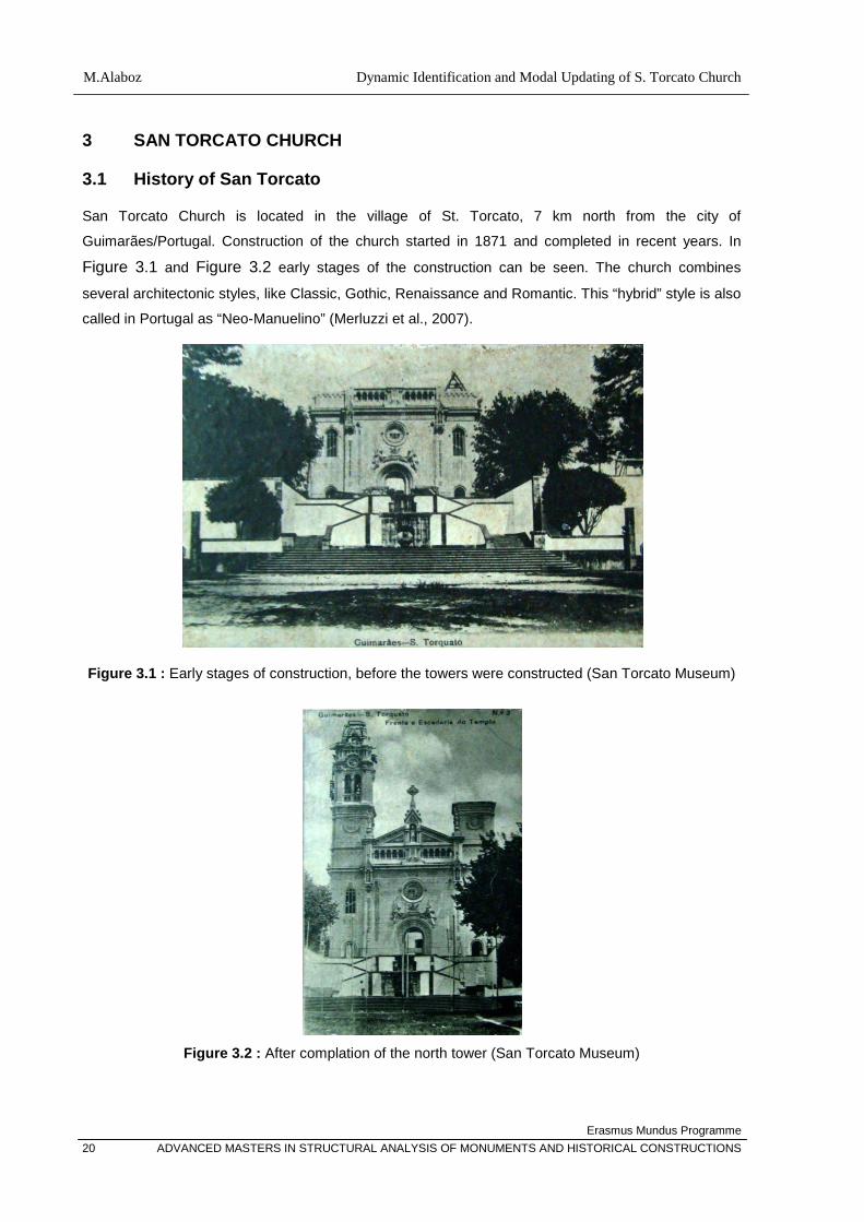
M.Alaboz Dynamic Identification and Modal Updating of S. Torcato Church
Erasmus Mundus Programme 20 ADVANCED MASTERS IN STRUCTURAL ANALYSIS OF MONUMENTS AND HISTORICAL CONSTRUCTIONS
3 SAN TORCATO CHURCH
3.1 History of San Torcato
San Torcato Church is located in the village of St. Torcato, 7 km north from the city of
Guimarães/Portugal. Construction of the church started in 1871 and completed in recent years. In
Figure 3.1 and Figure 3.2 early stages of the construction can be seen. The church combines
several architectonic styles, like Classic, Gothic, Renaissance and Romantic. This “hybrid” style is also
called in Portugal as “Neo-Manuelino” (Merluzzi et al., 2007).
Figure 3.1 : Early stages of construction, before the towers were constructed (San Torcato Museum)
Figure 3.2 : After complation of the north tower (San Torcato Museum)

Dynamic Identification and Modal Updating of S. Torcato Church M.Alaboz
Erasmus Mundus Programme ADVANCED MASTERS IN STRUCTURAL ANALYSIS OF MONUMENTS AND HISTORICAL CONSTRUCTIONS 21
3.2 Structural Definition of the church
Architectural plan shape of San Torcato Church exhibits a classical cross shape basilica scheme
(Figure 3.3) with the main nave covered with a barrel vault, transept that is crowned with a dome in
the middle and the apse part. Besides the main facade two towers are located. Between towers and
transepts one story low height additional buildings are situated. Accesses to the towers are provided
from inside those buildings.
Figure 3.3 : Gound level plan (UMinho, Civil Engineering Dept.,1999)
Main nave of the church is 57.5 × 17.5 m in length and it has 26.5 m height. There is a balcony in the
level of 7 m above the ground level which connects the two towers to each other. Balcony is supported
by main facade, towers and double arches on the side of nave (Figure 3.4).
Figure 3.4 : Balcony of the church

M.Alaboz Dynamic Identification and Modal Updating of S. Torcato Church
Erasmus Mundus Programme 22 ADVANCED MASTERS IN STRUCTURAL ANALYSIS OF MONUMENTS AND HISTORICAL CONSTRUCTIONS
Main nave is covered with a masonry barrel vault (Figure 3.5). Thickness of the vault is 0.45 m and
additional concrete cover is constructed upon it which is around 0.30 m thick. Quality of the concrete
can be interpreted as poor, considering the construction time and aggregate inside. It contains
crumbled stone and tile pieces and constructed without steel bars.
Figure 3.5 : Main nave and arch supported barrel vault
Main nave is supported by four single and one double stone arches which stand on stone columns.
Stone columns are supported with buttresses adjacent to body walls of the nave. As the supporting
arches are stone, a superficial layer of concrete is observed on arches and the vault. On the transition
with transept, main dome is carried by a masonry double arch.
The buttresses which support the arches extend till the level roof, about 5 m higher than the springing
of the vault. Beams of the timber framed suspended roof are carried by those pillars (Figure 3.6).
Figure 3.6 : Timber roof and stone pillars that carry the roof

Dynamic Identification and Modal Updating of S. Torcato Church M.Alaboz
Erasmus Mundus Programme ADVANCED MASTERS IN STRUCTURAL ANALYSIS OF MONUMENTS AND HISTORICAL CONSTRUCTIONS 23
In the level of vault springing, a balcony is located on the side of facade. Prominent damages are easy
to observe mostly in that part of the structure.
The transept of the church is 37.1 × 11.4 m in dimensions. Body walls of the transept have the
thickness 2.30 m and are made of stone. It is covered with vaults that are carried by 3 arches which
stand on stone columns. Roof of the transept is covered with timber framed suspend roof like in the
main nave, while in the middle a steel ribbed dome situated. Dome is supported with stone double
arches in four directions. Base of the dome is consists of modern reinforced concrete.
In the apse, different types of construction techniques are observed. While the vault was constructed
with stone, it was covered with a reinforced concrete layer. 8 to 10 mm diameter steel meshes were
used to reinforce (Figure 3.7). Body walls of the apse were constructed with stone till the springing
level of the vault. In the springing of the supporting arches, reinforced concrete beams were used
which aim to transfer lateral thrust of the arches to body walls. Roof of the transept consisted of timber
framed suspend roof.
After the level of springing, walls of apse were constructed with reinforced concrete. Facade of the
apse was covered with a 15 cm vein of stone.
Figure 3.7 : Reinforced concrete cover of the apse vault and concrete walls
Bell-towers have a cross section equal to 7.5 × 6.3 m2 with approximately 50 m height. They provide
entrance to the church on the ground level and the stone stairs allow accesses to belfries and
balconies.

M.Alaboz Dynamic Identification and Modal Updating of S. Torcato Church
Erasmus Mundus Programme 24 ADVANCED MASTERS IN STRUCTURAL ANALYSIS OF MONUMENTS AND HISTORICAL CONSTRUCTIONS
3.3 Structural Damages
Due to long duration of construction, structural techniques and materials vary within whole structure.
The main façade, towers beside the façade and main nave are prior in construction phase and made
of granite stone with dry joints while the apse is combined with reinforced concrete walls after the
springing level of the vault.
The significant structural problem of the structure is the crack pattern on the main facade due to
inclination of towers. The crack seen on the main facade is starting from the mid arch of the entrance
and goes to through the circular window and reaches to the left corner of tympanum (Figure 3.8).
Continuity of cracks inside the church and tilting of the towers indicates a settlement due to high stress
level of towers and soft filling layer of soil.
Figure 3.8 : Crack pattern on main facade
Extension of the cracks is observed even inside the church. On the interior balcony, cracks divide the
floor into three parts with longitudinal cracks (see Figure 3.9). On the north part of the nave, just
below and above the arched window which is close to the tower, has cracks in vertical direction. Crack
starts form the ground and continue till the top of the window. The cracks seen on the facade tear the
whole wall section.
As it can be justified by the crack pattern, inclination of towers due to soil settlement is the source of
damages on the structure. Moreover, on the walls of towers near to the ground hairline cracks are
visible which might be occurred due to high compression.

Dynamic Identification and Modal Updating of S. Torcato Church M.Alaboz
Erasmus Mundus Programme ADVANCED MASTERS IN STRUCTURAL ANALYSIS OF MONUMENTS AND HISTORICAL CONSTRUCTIONS 25
a) b)
Figure 3.9 : a) Crack on the floor of balcony and b) the crack on the facade wall
3.4 Previous Investigations
In order to obtain more reliable information about the sources of damages and safety assessment of
the structure, an investigation campaign was started in 1998 and still goes on.
3.4.1 Standart Penetration Dynamic Test (1998-99)
To represent the characteristics of strength and deformability of soil, standard penetration test was
carried out in 31 locations for a depth of up to 8m around the tower and up to 4m at the transept area.
The result of the test showed that at the vicinity of the tower the presence of layers of soil from landfill
earth with extraordinarily low mechanical properties was found (Merluzzi et al.,2007).
Figure 3.10 : Soil section according to investigation results

M.Alaboz Dynamic Identification and Modal Updating of S. Torcato Church
Erasmus Mundus Programme 26 ADVANCED MASTERS IN STRUCTURAL ANALYSIS OF MONUMENTS AND HISTORICAL CONSTRUCTIONS
3.4.2 Static Monitoring (1999)
In 1999 several monitoring records were taken aiming to monitor the openings of cracks and the
inclination of the towers. For this purpose, cracks meters were used in 14 points to check whether the
cracks are active, tiltometer was used to monitor the inclination of the tower and additionally
displacements were recorded (Merluzzi et al,2007). Using a Clinometers installed in each tower, the
angle of the towers were measured. According to the latest monitoring results (June - 2009) the slope
of the towers, left towers is 9x10⁻² rad and right tower is 9x10⁻² rad.
Figure 3.11 : Crack monitoring
Figure 3.12 : Inclination measurements with tiltometer

Dynamic Identification and Modal Updating of S. Torcato Church M.Alaboz
Erasmus Mundus Programme ADVANCED MASTERS IN STRUCTURAL ANALYSIS OF MONUMENTS AND HISTORICAL CONSTRUCTIONS 27
3.4.3 Displacement Monitoring (1999)
Using an optical Theodolite – total station the displacement of the towers, floor and arches of the nave
had been recorded. The results of the recording were as follows:
• the bell towers are tilting with transverse displacements;
• the inclinations are of the order of 8 × 10⁻⁴ rad for the left tower and 12 × 10-4 rad for the
right tower
• the arches in the main nave and the ground floor showed vertical deformations (Merluzzi et
al., 2007).
3.4.4 Dynamic Identification (2007)
A dynamic investigation on two towers and the main façade of the St. Torcato church were carried out
in 2007 to perform preliminary dynamics identification (Ramos & Aguilar,2007).
Towers were measured in X – Y directions at each corner. Balcony on the main facade was measured
only in Y direction to capture out of plane behaviour. During the tests four accelerometers were used
and measurements were taken as separated experiments. Only in towers in order to measure 8 DOF,
two in each corner, 3 setups were taken. For all measured points and on each test setup, 10 minutes
of data were acquired and with the sampling frequency 2000 Hz (Ramos & Aguilar,2007).
Figure 3.13 : Placement of accelerometers on towers and order of setups
Figure 3.14 : Placement of accelerometers on balcony

M.Alaboz Dynamic Identification and Modal Updating of S. Torcato Church
Erasmus Mundus Programme 28 ADVANCED MASTERS IN STRUCTURAL ANALYSIS OF MONUMENTS AND HISTORICAL CONSTRUCTIONS
The results of separate measurements taken in towers exhibit very close frequency estimations (see
Table 3.1). However, while the balcony has closer frequency values in first two modes, third and forth
frequencies have higher values which can be interpreted as local modes.
Table 3.1 : Frequency and damping estimation of north tower (Ramos & Aguilar,2007)
Mode Frequency [Hz] Std. Frequency [Hz] Damping Ratio
[%] Std. Damping
Ratio [%] Mode 1 2.13 0.01063 1.249 0.1106 Mode 2 2.601 0.01276 1.717 0.5385 Mode 3 2.821 0.00721 0.893 0.1874 Mode 4 2.917 0.01012 1.055 0.1796
Mode 1 Mode 2 Mode 3 Mode 4
Figure 3.15 : Mode shapes of north tower
Table 3.2 : Frequency and damping estimation of south tower (Ramos & Aguilar, 2007)
Mode Frequency [Hz] Std. Frequency [Hz] Damping Ratio
[%] Std. Damping
Ratio [%] Mode 1 2.138 0.005446 1.164 0.1204 Mode 2 2.615 0.004724 1.269 0.2297 Mode 3 2.849 0.002391 0.9843 0.1127 Mode 4 2.901 0.01204 1.506 1.216
Mode 1 Mode 2 Mode 3 Mode 4
Figure 3.16 : Mode shapes of south tower (Ramos&Aguilar,2007)

Dynamic Identification and Modal Updating of S. Torcato Church M.Alaboz
Erasmus Mundus Programme ADVANCED MASTERS IN STRUCTURAL ANALYSIS OF MONUMENTS AND HISTORICAL CONSTRUCTIONS 29
Table 3.3 : Frequency and damping estimation of facade (Ramos & Aguilar, 2007)
Mode Frequency [Hz]
Damping Ratio [%]
Mode 1 2.58 2.2 Mode 2 2.93 2.5 Mode 3 4.06 6.4 Mode 4 4.34 7.3
Mode 1 Mode 2
Mode 3 Mode 4
Figure 3.17 : Mode shapes of balcony (Ramos & Aguilar, 2007)
When the mode shapes of the towers are examined, first and second mode exhibit translational
modes in X and Y direction. Third and forth mode shapes exhibit more complex behaviour.
Mode shapes of balcony part gives an idea about the effect of damages in that part. Balcony part is
significantly damaged. First mode shape of the balcony exhibits torsional movement. While the first
mode shape of the towers are in X direction, out of plane behaviour of facade can be related with the
damages. Even in the second mode non uniform movement in Y direction is observed.

M.Alaboz Dynamic Identification and Modal Updating of S. Torcato Church
Erasmus Mundus Programme 30 ADVANCED MASTERS IN STRUCTURAL ANALYSIS OF MONUMENTS AND HISTORICAL CONSTRUCTIONS
4 DYNAMIC IDENTIFICATION OF SAN TORCATO CHURCH
Following the previous works, a comprehensive dynamic identification test were taken in 2009 aiming
to identify global dynamic properties of the structure, soil-structure interaction, structural bonding at
joints of different phases and influence of bell swinging. Furthermore, the collected data is supposed
to be used for modal updating of a previously prepared finite element model and provide information
for the planning of dynamic monitoring.
4.1 Data Acquisition System
In experimental modal analysis of San Torcato Church, 10 uniaxial PCB 393B12 model piezolectric
accelerometers with a bandwidth ranging from 0.15 to 1000 Hz (5%), a dynamic range of ±0.5 g,
sensitivity of 10 V/g, 8 μg of resolution and 210 gr of weight were used. For data acquiring, a 16
channel Digital to Analogue Converter (ADC) was used (Figure 2.1).
a) b)
Figure 4.1 : a) Accelerometer used in test and b) DAQ system
4.2 Test Planning
Before the experimental test is taken in the field, prior estimation of expected frequencies and decision
of measurement points, reference points were studied, to prevent any mistakes that cannot be
corrected with no signal processing and loose of time. For this purpose, previous FE model and
preliminary test result were considered.
For the expected frequency range, preliminary test results were taken into account, as it was shown in
the Section 3.4.4, the first four frequencies are between 2-3 Hz. For the measurement points and
reference points, mode shapes of the FE model and general engineering judgement were affective on
decisions.
Reference accelerometers were decided to place at towers because of their high amplitude and
contribution in each mode. Towers and main facade had to be measured with precisely as they have
serious damages. Thus, the amount of measurement points was chosen dense. Main nave of the
structure as well decided to be measured in 13 points at the support of the vault and top of the vault.

Dynamic Identification and Modal Updating of S. Torcato Church M.Alaboz
Erasmus Mundus Programme ADVANCED MASTERS IN STRUCTURAL ANALYSIS OF MONUMENTS AND HISTORICAL CONSTRUCTIONS 31
Transept was decided to be measured at the corners one in X one in Y direction. In apse part, corners
and one additional points in the mid of wings were decided to be measured to capture flexural
movements (see Figure 4.5, Figure 4.2 and Figure 4.4).
Figure 4.2 : Data acquisition system set on the main nave
Totally, 9 setups and 35 points were decided to be measured. However, during the experiment, due to
lack of cables and accessibility problems, distribution of DOF’s in setups and even the measurement
points were changed.
During the experiments, ambient vibration was used for excitation source. The wind and traffic
excitation was enough to obtain at least first four mode for all structure. In addition to ambient
vibration, impact hammer was used in the nave and on the belfry of north tower. During bell swinging
one setup records were taken separately. Bells were not controlled electronically, so the frequency of
swinging was not highly controlled.
Reference transducers were placed in different points in two directions at the towers (see Figure 4.3).
Each towers were measured in 6 points in two levels, belfry and on the stairs in the level of main vault
springing (P1, P2 and P3 in left belfry, P11, P12 and P13 in left stair level, P4, P5 and P6 in right
belfry , P19, P20 and P21 in right stair level) (Figure 4.4). In all setups, symmetry on east-west
direction was considered to check if the existing damage caused some separations on the church.

M.Alaboz Dynamic Identification and Modal Updating of S. Torcato Church
Erasmus Mundus Programme 32 ADVANCED MASTERS IN STRUCTURAL ANALYSIS OF MONUMENTS AND HISTORICAL CONSTRUCTIONS
Figure 4.3 : Measured DOFs in towers.
Figure 4.4 : Measured DOFs in stair level and balcony
Five accelerometers were placed on balcony where the damage is observed significantly and
measured only in X direction to define out of plane behaviour (P14, P15, P16, P17, and P18) (Figure
4.4).
On the main nave, in the level of skewbacks, 4 points were measured in each side (P22, P23, P24
and P25 on the right, P26, P27, P28 and P29). Direction of the measurements in the middle of the
nave was decided to be in Y direction to catch out of plane movements. In the corners of the dome
(P29, P25, P30, P35), and in the points close to the towers (P26, P22), measurements were taken in
two directions (Figure 4.5).
In the transept, measurements were taken in the level roof, on the corners in X and Y direction (P7,
P8, P9, P10). In the apse, records were taken on the cornice level due to inaccurate measurement of
the movement on parapets. In the corners of the apse, measurements were taken in two directions
(P30, P32, P33, P35). In the middle of the apse, records were taken on Y direction to catch out of
plane movements (P31, P34) (Figure 4.5).

Dynamic Identification and Modal Updating of S. Torcato Church M.Alaboz
Erasmus Mundus Programme ADVANCED MASTERS IN STRUCTURAL ANALYSIS OF MONUMENTS AND HISTORICAL CONSTRUCTIONS 33
DAQ System was placed on the main nave in order to be in same distance from the measurement
points (between P39 and P40) .
Figure 4.5 : Plan of measured DOFs
Table 4.1 : The chart that shows the measured DOF’s with their direction in each setup
Ch 1 Ch 2 Ch 3 Ch 4 Ch 5 Ch 6 Ch 7 Ch 8 Ch 9 Ch 10
Ref 1 Ref 2 Ref 3 Ref 4 Mov 1 Mov 2 Mov 3 Mov 4 Mov 5 Mov 6
Setup 1 P1 / -Y P2 / +X P4 / -Y P5 / +X P3 / +Y P6 / +Y P20 / +Y P12 / -Y P 39 / -Y P40 / -X Setup 2 P1 / -Y P2 / +X P4 / -Y P5 / +X P11 / -X P19 / -X P21 / +Y P13 / +X P22 / +X P26 / +X Setup 3 P1 / -Y P2 / +X P4 / -Y P5 / +X P22 / +Y P23 / +Y P24 / +Y P26 / +Y P27 / +Y P28 / +Y Setup 4 P1 / -Y P2 / +X P4 / -Y P5 / +X P25 / +Y P25 / +X P29 / +Y P29 / +X P37 / +Y - Setup 5 P1 / -Y P2 / +X P4 / -Y P5 / +X P14 / -X P15 / -X P16 / -X P17 / -X P18 / -X P36 / +Y Setup 6 P1 / -Y P2 / +X P4 / -Y P5 / +X P30 / +X P30 / +Y P31 / +X P31 / -Y - - Setup 7 P1 / -Y P2 / +X P4 / -Y P5 / +X P32 / +X P32 / +Y P33 / +X P33 / +Y - - Setup 8 P1 / -Y P2 / +X P4 / -Y P5 / +X P34 / +X P34 / +Y - - - - Setup 9 P1 / -Y P2 / +X P4 / -Y P5 / +X P35 / +X P35 / +Y - - - -
In each point, measurements were taken for 10 minutes with 200 Hz frequency. Setups were
measured 2-3 times to avoid any possible mistakes may happen when acquiring and also to be able to
choose best quality recorded data (considering the noise level of the records).
For data processing, output-only techniques were used. Recorded signals were processed with FDD
and SSI techniques.
In addition to frequency estimation, bell excitement and impact hammer test were used to estimate the
damping of the structure. For the estimation of soil properties, soil measurements were taken in 4

M.Alaboz Dynamic Identification and Modal Updating of S. Torcato Church
Erasmus Mundus Programme 34 ADVANCED MASTERS IN STRUCTURAL ANALYSIS OF MONUMENTS AND HISTORICAL CONSTRUCTIONS
points in 3 directions. Measurements taken for 30 min for each setup and 500 Hz sampling frequency
was used.
For FFT and SSI analysis, specialized signal processing software Artemis Extractor Pro 2009 Release
4.5 was used. Beside the software, acceleration-time graphs were plotted and RMS values were
calculated with a computational software Matlab code (MATLAB, 2007).
4.3 Preliminary Analysis of Setups
Each setup was processed with different methods in order to check the results and increase the level
of confidence. In processing of the signals, frequency domain methods and stochastic methods were
used which are implemented in the software Artemis (Artemis, 2009)
In FDD technique each mode is estimated as a decomposition of the system's response spectral
densities into several single-degrees-of-freedom (SDOF) systems. For frequency domain analysis,
frequency range of processes was 0-20 Hz with 1024 points window length. Although software can
estimate the frequencies automatically, peaks were picked manually.
To compare the results with other frequency domain techniques EFDD and CFDD methods which are
explained in allow the estimation of the damping ratio as an extra feature as well as the estimation of
eigenfrequencies independent of the frequency resolution.
The SSI method is based on state space matrices explained before. As an addition to common SSI
analysis, input matrix is weighted that consist of compressed time series data. The method called as
SSI-PC (stochastic subspace identification- principal component).
For the SSI analysis, SSI-PC method was used. Maximum state space dimension for estimations were
selected as 100. Original data was used without decimation.
The acceleration-time graphs of each setup are given above in Figure 4.6, Figure 4.7 and in Figure
4.8. Several measurements were taken in each setup in order to choose the best quality record. As it
can be seen in the graphs, mostly the ambient excitation level for sampling duration is regular.
Besides, in Setup 7 and Setup 9 (see Figure 4.7 and Figure 4.8) due to bell swinging very high solitary
peaks are seen. Nevertheless, short time occurrence of the events cannot disturb the quality of
records.

Dynamic Identification and Modal Updating of S. Torcato Church M.Alaboz
Erasmus Mundus Programme ADVANCED MASTERS IN STRUCTURAL ANALYSIS OF MONUMENTS AND HISTORICAL CONSTRUCTIONS 35
Setup 1
Setup 2
Setup 3
Setup 4
Figure 4.6 : Acceleration time graphs of Setup 1 – Setup 4

M.Alaboz Dynamic Identification and Modal Updating of S. Torcato Church
Erasmus Mundus Programme 36 ADVANCED MASTERS IN STRUCTURAL ANALYSIS OF MONUMENTS AND HISTORICAL CONSTRUCTIONS
Setup 5
Setup 6
Setup 7
Setup 8
Figure 4.7 : Acceleration time graphs of Setup 5 – Setup 8
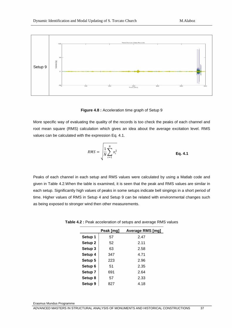
Dynamic Identification and Modal Updating of S. Torcato Church M.Alaboz
Erasmus Mundus Programme ADVANCED MASTERS IN STRUCTURAL ANALYSIS OF MONUMENTS AND HISTORICAL CONSTRUCTIONS 37
Setup 9
Figure 4.8 : Acceleration time graph of Setup 9
More specific way of evaluating the quality of the records is too check the peaks of each channel and
root mean square (RMS) calculation which gives an idea about the average excitation level. RMS
values can be calculated with the expression Eq. 4.1.
𝑅𝑅𝑀𝑀𝑆𝑆 = �1𝑁𝑁�𝑥𝑥𝐵𝐵2𝑁𝑁
𝐵𝐵=1
Eq. 4.1
Peaks of each channel in each setup and RMS values were calculated by using a Matlab code and
given in Table 4.2.When the table is examined, it is seen that the peak and RMS values are similar in
each setup. Significantly high values of peaks in some setups indicate bell singings in a short period of
time. Higher values of RMS in Setup 4 and Setup 9 can be related with environmental changes such
as being exposed to stronger wind then other measurements.
Table 4.2 : Peak acceleration of setups and average RMS values
Peak [mg] Average RMS [mg] Setup 1 57 2.47 Setup 2 52 2.11 Setup 3 63 2.58 Setup 4 347 4.71 Setup 5 223 2.96 Setup 6 51 2.35 Setup 7 691 2.64 Setup 8 57 2.33 Setup 9 827 4.18

M.Alaboz Dynamic Identification and Modal Updating of S. Torcato Church
Erasmus Mundus Programme 38 ADVANCED MASTERS IN STRUCTURAL ANALYSIS OF MONUMENTS AND HISTORICAL CONSTRUCTIONS
Setup 1
Setup 2
Setup 3
Setup 4
Figure 4.9 : Frequency decomposition graph of Setup 1 to Setup 4

Dynamic Identification and Modal Updating of S. Torcato Church M.Alaboz
Erasmus Mundus Programme ADVANCED MASTERS IN STRUCTURAL ANALYSIS OF MONUMENTS AND HISTORICAL CONSTRUCTIONS 39
Setup 5
Setup 6
Setup 7
Setup 8
Figure 4.10 : Frequency decomposition graph of Setup 5 to Setup 8

M.Alaboz Dynamic Identification and Modal Updating of S. Torcato Church
Erasmus Mundus Programme 40 ADVANCED MASTERS IN STRUCTURAL ANALYSIS OF MONUMENTS AND HISTORICAL CONSTRUCTIONS
Setup 9
Figure 4.11 : Frequency decomposition graph of Setup 9
Frequency response graphs are very useful to see interpret the data roughly. As it can be seen in the
figures above (Figure 4.9, Figure 4.10 and Figure 4.11), the peaks are indicating resonant
frequencies.
When the graphs are examined, in each setup between 2 to 3 Hz clear peaks are identified. Although
their amplitude changes from one to the other, main frequencies are expected in this range.
In the first 6 setups which are taken in the oldest part of the structure (the part starting from facade to
transept) some other peaks are visible in the range of 4 to 5 Hz. However, to be able to talk about
global frequencies, all the setups should be processed together.
In Table 4.3 frequency estimation of setups with FDD method is given. Each setup was calculated
separately and the peaks were picked manually.
Table 4.3 : Frequency estimation of setups by FDD method
Setup 1 Setup 2 Setup 3 Setup 4 Setup 5 Setup 6 Setup 7 Setup 8 Setup 9 Mode 1 2.09 2.62 2.17 2.21 2.19 2.09 2.11 2.13 2.19 Mode 2 2.60 2.85 2.64 2.70 2.68 2.58 2.59 2.61 2.60 Mode 3 2.83 2.93 2.97 3.01 2.89 2.89 2.81 2.90 2.86 Mode 4 5.04 4.94 4.24 4.28 4.28 4.14 2.90 4.13 2.92 Mode 5 5.53 - 5.70 4.79 4.53 4.94 4.20 4.92 5.73 Mode 6 - - - 5.22 - 5.82 4.93 6.15 7.16 Mode 7 - - - - - - - 7.18 -

Dynamic Identification and Modal Updating of S. Torcato Church M.Alaboz
Erasmus Mundus Programme ADVANCED MASTERS IN STRUCTURAL ANALYSIS OF MONUMENTS AND HISTORICAL CONSTRUCTIONS 41
4.4 Processing of All Setups
After the first data processing for quality check it was concluded at least, first four modes of the
structure are presented in all setups. Higher modes are visible in some setups; however, the peaks
are not clear enough to allow accurate estimation. Next; of this modes combined analysis of all 9
setups are presented with the comparison of different methods.
4.4.1 Frequency Domain Decomposition
As can be seen in Figure 4.12, peaks of the spectral density matrices of the FDD method are mostly
concentrated below 4 Hz. Others peaks are visible between 4 Hz and 8 Hz. For more accurate
estimations, data must be processed with SSI methods which give better results in case of having
close peaks.
Figure 4.12 : Frequency decomposition of setups and picked peaks
Table 4.4 : Frequency estimation of all setups
Modes Frequency [Hz]
FDD Mode 1 2.148
FDD Mode 2 2.637 FDD Mode 3 2.891 FDD Mode 4 2.969
4.4.2 Enhanced FDD
The EFDD method allows damping estimation by inverse Fourier transformation. Figure 4.13
shows the peaks and Table 4.5 presents the frequency values, values for both damping and
frequency, calculated for each setup. Standard frequency variation is around 0.05 which
shows that the estimation error for frequencies is very low. Nevertheless, the variation of
damping ratio and standard variation values are relatively high with the maximum value of
0.74. Thus, the efficiency of the EFDD method is acceptable when the estimation of damping
is not sufficient.

M.Alaboz Dynamic Identification and Modal Updating of S. Torcato Church
Erasmus Mundus Programme 42 ADVANCED MASTERS IN STRUCTURAL ANALYSIS OF MONUMENTS AND HISTORICAL CONSTRUCTIONS
Figure 4.13 : EFDD graph of all setups and picked peaks
Table 4.5 : EFDD method frequency and damping estimations for all setups and their standard variation
Mode Frequency [Hz]
Std. Frequency [Hz]
Damping Ratio [%]
Std. Damping Ratio [%]
EFDD Mode 1 2.14 0.04 1.78 0.61 EFDD Mode 2 2.62 0.05 1.45 0.45 EFDD Mode 3 2.89 0.04 0.77 0.74 EFDD Mode 4 2.94 0.04 0.79 0.27 4.4.3 Curve-Fit FDD
Curve-fit frequency domain decomposition method implemented in Artemis software, use the same
procedure for the calculation of FDD for peak picking. Then each frequency converted in to SDOF
Spectra Bell. Damping estimation is performed where the mode shape vectors in convergence.
Resultant frequencies are obtained by averaging of FDD and SDOF frequencies (Artemis Release
4.5).
The CFDD spectrum results are presented in Figure 4.14, where the selected peaks of the resonant
frequencies are shown. The estimated values for frequencies and damping ratios are presented in
Table 4.6.
Figure 4.14 : CFDD frequency domain graph and picked peaks
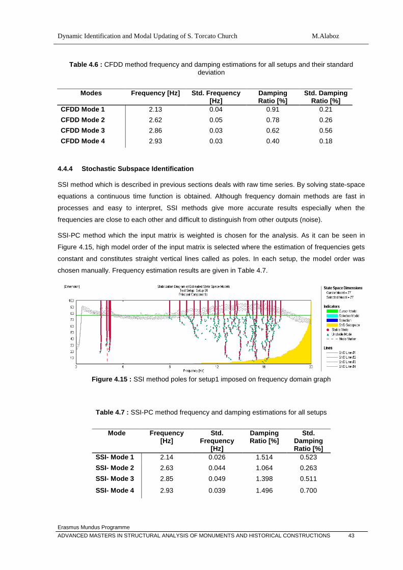
Dynamic Identification and Modal Updating of S. Torcato Church M.Alaboz
Erasmus Mundus Programme ADVANCED MASTERS IN STRUCTURAL ANALYSIS OF MONUMENTS AND HISTORICAL CONSTRUCTIONS 43
Table 4.6 : CFDD method frequency and damping estimations for all setups and their standard deviation
Modes Frequency [Hz] Std. Frequency
[Hz] Damping Ratio [%]
Std. Damping Ratio [%]
CFDD Mode 1 2.13 0.04 0.91 0.21 CFDD Mode 2 2.62 0.05 0.78 0.26 CFDD Mode 3 2.86 0.03 0.62 0.56 CFDD Mode 4 2.93 0.03 0.40 0.18
4.4.4 Stochastic Subspace Identification
SSI method which is described in previous sections deals with raw time series. By solving state-space
equations a continuous time function is obtained. Although frequency domain methods are fast in
processes and easy to interpret, SSI methods give more accurate results especially when the
frequencies are close to each other and difficult to distinguish from other outputs (noise).
SSI-PC method which the input matrix is weighted is chosen for the analysis. As it can be seen in
Figure 4.15, high model order of the input matrix is selected where the estimation of frequencies gets
constant and constitutes straight vertical lines called as poles. In each setup, the model order was
chosen manually. Frequency estimation results are given in Table 4.7.
Figure 4.15 : SSI method poles for setup1 imposed on frequency domain graph
Table 4.7 : SSI-PC method frequency and damping estimations for all setups
Mode Frequency
[Hz] Std.
Frequency [Hz]
Damping Ratio [%]
Std. Damping Ratio [%]
SSI- Mode 1 2.14 0.026 1.514 0.523 SSI- Mode 2 2.63 0.044 1.064 0.263 SSI- Mode 3 2.85 0.049 1.398 0.511
SSI- Mode 4 2.93 0.039 1.496 0.700

M.Alaboz Dynamic Identification and Modal Updating of S. Torcato Church
Erasmus Mundus Programme 44 ADVANCED MASTERS IN STRUCTURAL ANALYSIS OF MONUMENTS AND HISTORICAL CONSTRUCTIONS
4.4.5 Comparison of Methods
Frequency estimation of the recorded data for all setups combined and processed together. In the
processes, different modal identifications were used to validate the results (Table 4.8). Frequency
difference of the methods shows the efficiency of methods in frequencies (Table 4.9). However, the
variation of damping ratio estimations present high differences. As it was explained in previous
sections each method has a different damping estimation processes. Estimated values are given in
Table 4.10.
Table 4.8 : Frequency estimations of different identification methods [Hz]
FDD EFDD CFDD SSI
Mode 1 2.15 2.14 2.13 2.14
Mode 2 2.64 2.62 2.62 2.63
Mode 3 2.89 2.89 2.86 2.85
Mode 4 2.97 2.94 2.93 2.93 SSI method gives more accurate results due to processing in time domain data, especially where the
peaks are close to each other in frequency domain. Thus, SSI results used to to compare the result of
other methods. Table 4.10 gives the error ratio in frequencies.
Table 4.9 : Frequency error of different methods based on SSI values
Frequency Error of Methods
SSI [Hz] FDD [%] EFDD [%] CFDD [%]
Mode 1 2.14 0.4 0.1 0.3 Mode 2 2.63 0.4 0.1 0.1 Mode 3 2.85 1.3 1.1 0.3 Mode 4 2.93 1.4 0.3 0.1
Table 4.10 : Damping estimation and standard variation of different methods
EFDD CFDD SSI
Damping Ratio [%]
Std. Damping Ratio [%]
Damping Ratio [%]
Std. Damping Ratio [%]
Damping Ratio [%]
Std. Damping Ratio [%]
Mode 1 1.78 0.61 0.91 0.21 1.51 0.52 Mode 2 1.45 0.45 0.78 0.26 1.06 0.26 Mode 3 0.77 0.74 0.62 0.56 1.40 0.51
Mode 4 0.79 0.27 0.40 0.18 1.50 0.70

Dynamic Identification and Modal Updating of S. Torcato Church M.Alaboz
Erasmus Mundus Programme ADVANCED MASTERS IN STRUCTURAL ANALYSIS OF MONUMENTS AND HISTORICAL CONSTRUCTIONS 45
4.4.6 Mode Shape Presentation
After estimation of frequencies, Artemis software allow user to see the mode shapes. For this purpose,
a simplified geometric model was constructed and measurement points were defined with their
directions. As it was discussed, movement of non measured DOF’s of the model were correlated by
introducing some slave equations. Thus, the movement of non measured points were simulated
depending on other points.
First two mode of the structure is observed as translational modes in X and Y directions. Even though,
the whole structure is moving together, towers have higher amplitudes due to their flexibility (Figure
4.16-a and Figure 4.16-b).
Third and forth mode of the structure exhibits torsion modes. Towers move diagonally in opposite
directions while the nave flex (Figure 4.16-c and Figure 4.16-d).
Mode 1 / 2.14 Hz Mode 2 / 2.63 Hz
Mode 3 / 2.85 Hz Mode 4 / 2.93
Figure 4.16 : Mode shapes of SSI method frequency estimations

M.Alaboz Dynamic Identification and Modal Updating of S. Torcato Church
Erasmus Mundus Programme 46 ADVANCED MASTERS IN STRUCTURAL ANALYSIS OF MONUMENTS AND HISTORICAL CONSTRUCTIONS
5 MODAL UPDATING
Numerical analysis methods are being intensively used in design and assessment of structures. As
the computer technology develops the efficiency of models are increasing. However, when the
numerical predictions are compared with some experimental results the coherence may fall out of
confidence limits. (Friswell et al, 2009).
The numerical model of San Torcato Church was constructed to be used to use in static non-linear
analysis to evaluate intervention proposals. However, reliability of the model has a significant
importance in decision taking for any intervention. In that point, the correlation between experimental
modal responses and the response of the numerical model should be examined. In case of insufficient
correlation, tuning of numerical model by using robust optimization methods comes to picture.
Depending on the knowledge level, numerical model consists of several assumptions, including
geometric simplifications, estimation of mechanical properties, homogenization and linearization
judgements. Those steps of modelling may cause improper definitions as listed below;
• Model Structure Errors: Errors, liable to occur when the physical definitions are uncertain or
due to neglected non-linear behaviours,
• Model Parameter Errors : Contains the application of inappropriate boundary conditions and
any assumptions used in order to simplify the model,
• Model Order Errors: Errors arise in the discretization of complex systems. Commonly faced
when generating the meshes of models.
However, inaccuracy and incompatibility is an expected phenomenon. Thus, the studies on modelling
methods based on experimental results come to picture, called as system identification. The studied
model can be parametric or non-parametric, linear or non-linear.
When identifying a parametric model, once the model structure and model order have been decided,
then the parameters can be estimated. In structural dynamics, experimental modal analysis is used for
the determination of modal data (natural frequencies, mode shapes, generalized masses and damping
factors). In model updating generally batch processing techniques are used to generate improved
numerical models in order to obtain predictions for modified structural configurations. However, the
mass, stiffness and damping parameters in the updated model should be physically meaningful
(Mottershead & Friswell, 1993).
5.1 Modal Assurance Criterion
Due to frequency response function matrix contain redundant information with respect to a modal
vector, estimation of the modal vector for varying conditions or modal parameter estimation algorithms
become valuable confidence factor of evaluation of experimental modal vectors (Allemang, 2003).

Dynamic Identification and Modal Updating of S. Torcato Church M.Alaboz
Erasmus Mundus Programme ADVANCED MASTERS IN STRUCTURAL ANALYSIS OF MONUMENTS AND HISTORICAL CONSTRUCTIONS 47
The function of the modal assurance criterion (MAC) provides a measure consistency (linearity)
between the estimated modal vectors. MAC is defined as in Eq. 5.1;
𝑀𝑀𝐴𝐴𝐶𝐶𝑢𝑢 ,𝑑𝑑 =�{𝜑𝜑𝐵𝐵𝑢𝑢}𝑇𝑇�𝜑𝜑𝐵𝐵𝑑𝑑��
2
{𝜑𝜑𝐵𝐵𝑢𝑢}𝑇𝑇{𝜑𝜑𝐵𝐵𝑢𝑢}{𝜑𝜑𝐵𝐵𝑑𝑑}𝑇𝑇{𝜑𝜑𝐵𝐵𝑑𝑑}
Eq. 5.1
Where 𝜑𝜑𝑢𝑢 and 𝜑𝜑𝑑𝑑 are the mode shape vector of two different models. MAC value will fall into a range
0 to 1, which 1 indicates 100% match of both mode shape vectors. Also it can be expressed as;
The modal assurance criterion is mostly used for validation of experimental results. In the same way it
is practical to evaluate the correlation between experimental and numerical models. For this purpose it
can give reasonable results for modal parameter estimation algorithms. In damage assessment and
optimal sensor placement it can be a useful tool.
Although MAC is judged as a useful tool for various cases, it should be stressed that in some cases
the results may mislead for wrong interpretations. In case of limited numbers of DOF’s are measured
and if the structure couldn’t be observed properly, high values of the method cannot be interpreted as
a good match. Even though, this method is sensitive for high magnitudes. When the higher
magnitudes have dominant effect on the results, erroneous points will have minor effects. Same
problem may occur when the numbers of measurement points are not enough or well distributed. In
order to have better results, DOF’s in modal vector should be excited equally which will address user
to choose proper comparison points (Allemang J. R., 2003).
5.2 The Coordinate Modal Assurance Criterion
In modal updating, while frequency differences can be related with basic material properties such as
elasticity modulus, MAC value differences may occur due to improper boundary condition definitions
or incomplete geometry definitions. COMAC values give the contribution of DOF’s as a summation of
all frequencies. Similar to MAC measure, values which are close to 1 indicates high consistency of
DOFs. COMAC value can be calculated by using the expression given in Eq. 5.2. (Allemang, 2003).
𝐶𝐶𝐶𝐶𝑀𝑀𝐴𝐴𝐶𝐶𝐵𝐵 ,𝑢𝑢 ,𝑑𝑑 =∑ �𝜑𝜑𝐵𝐵,𝑗𝑗𝑢𝑢 𝜑𝜑𝐵𝐵,𝑗𝑗𝑑𝑑 �
2𝑛𝑛𝐵𝐵
∑ �𝜑𝜑𝐵𝐵 ,𝑗𝑗𝑢𝑢 �
2𝑛𝑛𝐵𝐵 ∑ �𝜑𝜑𝐵𝐵 ,𝑗𝑗
𝑑𝑑 �2
𝑛𝑛𝐵𝐵
Eq. 5.2
5.3 Normalized Modal Difference
The Normalized Modal Difference (NMD) is dependent of the MAC values and evaluates the
difference of two mode shape vectors. The main difference from MAC is that NMD is more sensitive to
differences (Eq. 5.3). When the MAC value is below 0.90, NMD values will give higher values which
mean the difference is higher. Even with 0.99 of MAC, NMD evaluation will give 10% of difference. As
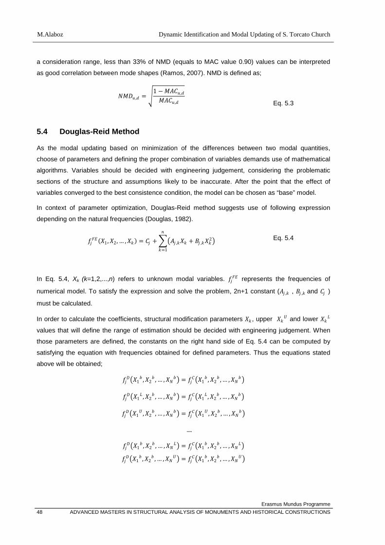
M.Alaboz Dynamic Identification and Modal Updating of S. Torcato Church
Erasmus Mundus Programme 48 ADVANCED MASTERS IN STRUCTURAL ANALYSIS OF MONUMENTS AND HISTORICAL CONSTRUCTIONS
a consideration range, less than 33% of NMD (equals to MAC value 0.90) values can be interpreted
as good correlation between mode shapes (Ramos, 2007). NMD is defined as;
𝑁𝑁𝑀𝑀𝐷𝐷𝑢𝑢 ,𝑑𝑑 = �1 −𝑀𝑀𝐴𝐴𝐶𝐶𝑢𝑢 ,𝑑𝑑
𝑀𝑀𝐴𝐴𝐶𝐶𝑢𝑢 ,𝑑𝑑
Eq. 5.3
5.4 Douglas-Reid Method
As the modal updating based on minimization of the differences between two modal quantities,
choose of parameters and defining the proper combination of variables demands use of mathematical
algorithms. Variables should be decided with engineering judgement, considering the problematic
sections of the structure and assumptions likely to be inaccurate. After the point that the effect of
variables converged to the best consistence condition, the model can be chosen as “base” model.
In context of parameter optimization, Douglas-Reid method suggests use of following expression
depending on the natural frequencies (Douglas, 1982).
𝑓𝑓𝑗𝑗𝐹𝐹𝐹𝐹(𝑋𝑋1,𝑋𝑋2, … ,𝑋𝑋𝑘𝑘) = 𝐶𝐶𝑗𝑗 + ��𝐴𝐴𝑗𝑗 ,𝑘𝑘𝑋𝑋𝑘𝑘 + 𝐵𝐵𝑗𝑗 ,𝑘𝑘𝑋𝑋𝑘𝑘2�𝑛𝑛
𝑘𝑘=1
Eq. 5.4
In Eq. 5.4, Xk (k=1,2,...,n) refers to unknown modal variables. 𝑓𝑓𝑗𝑗𝐹𝐹𝐹𝐹 represents the frequencies of
numerical model. To satisfy the expression and solve the problem, 2n+1 constant (𝐴𝐴𝑗𝑗 ,𝑘𝑘 , 𝐵𝐵𝑗𝑗 ,𝑘𝑘 and 𝐶𝐶𝑗𝑗 )
must be calculated.
In order to calculate the coefficients, structural modification parameters 𝑋𝑋𝑘𝑘 , upper 𝑋𝑋𝑘𝑘𝑈𝑈 and lower 𝑋𝑋𝑘𝑘𝐿𝐿
values that will define the range of estimation should be decided with engineering judgement. When
those parameters are defined, the constants on the right hand side of Eq. 5.4 can be computed by
satisfying the equation with frequencies obtained for defined parameters. Thus the equations stated
above will be obtained;
𝑓𝑓𝑗𝑗𝐷𝐷�𝑋𝑋1𝑏𝑏 ,𝑋𝑋2
𝑏𝑏 , … ,𝑋𝑋𝑁𝑁𝑏𝑏� = 𝑓𝑓𝑗𝑗𝐶𝐶�𝑋𝑋1𝑏𝑏 ,𝑋𝑋2
𝑏𝑏 , … ,𝑋𝑋𝑁𝑁𝑏𝑏�
𝑓𝑓𝑗𝑗𝐷𝐷�𝑋𝑋1𝐿𝐿 ,𝑋𝑋2
𝑏𝑏 , … ,𝑋𝑋𝑁𝑁𝑏𝑏� = 𝑓𝑓𝑗𝑗𝐶𝐶�𝑋𝑋1𝐿𝐿 ,𝑋𝑋2
𝑏𝑏 , … ,𝑋𝑋𝑁𝑁𝑏𝑏�
𝑓𝑓𝑗𝑗𝐷𝐷�𝑋𝑋1𝑈𝑈 ,𝑋𝑋2
𝑏𝑏 , … ,𝑋𝑋𝑁𝑁𝑏𝑏� = 𝑓𝑓𝑗𝑗𝐶𝐶�𝑋𝑋1𝑈𝑈 ,𝑋𝑋2
𝑏𝑏 , … ,𝑋𝑋𝑁𝑁𝑏𝑏�
....
𝑓𝑓𝑗𝑗𝐷𝐷�𝑋𝑋1𝑏𝑏 ,𝑋𝑋2
𝑏𝑏 , … ,𝑋𝑋𝑁𝑁𝐿𝐿� = 𝑓𝑓𝑗𝑗𝐶𝐶�𝑋𝑋1𝑏𝑏 ,𝑋𝑋2
𝑏𝑏 , … ,𝑋𝑋𝑁𝑁𝐿𝐿�
𝑓𝑓𝑗𝑗𝐷𝐷�𝑋𝑋1𝑏𝑏 ,𝑋𝑋2
𝑏𝑏 , … ,𝑋𝑋𝑁𝑁𝑈𝑈� = 𝑓𝑓𝑗𝑗𝐶𝐶�𝑋𝑋1𝑏𝑏 ,𝑋𝑋2
𝑏𝑏 , … ,𝑋𝑋𝑁𝑁𝑈𝑈�

Dynamic Identification and Modal Updating of S. Torcato Church M.Alaboz
Erasmus Mundus Programme ADVANCED MASTERS IN STRUCTURAL ANALYSIS OF MONUMENTS AND HISTORICAL CONSTRUCTIONS 49
The coefficients 𝐴𝐴𝑗𝑗 ,𝑘𝑘 , 𝐵𝐵𝑗𝑗 ,𝑘𝑘 and 𝐶𝐶𝑗𝑗 are calculated by means of stated equations. Afterwards, for the
minimization of differences of frequencies with experimental model, Eq. 5.5 is used.
𝐽𝐽 = �𝜔𝜔𝐵𝐵𝜀𝜀𝐵𝐵2𝑀𝑀
𝐵𝐵=1
Eq. 5.5
𝜀𝜀𝐵𝐵 = 𝑓𝑓𝐵𝐵𝑀𝑀 − 𝑓𝑓𝐵𝐵𝐷𝐷(𝑋𝑋1,𝑋𝑋2, … ,𝑋𝑋𝑁𝑁) Eq. 5.6
Error definition in Eq. 5.6 𝜀𝜀𝐵𝐵 is depending on the frequency errors. Solution of the objective function 𝐽𝐽
minimizes only the frequency errors. Furthermore, more robust formulation can be obtained by adding
modal displacement vectors and modal curvatures. Depending on the engineering judgement and
desired tuning outcome, weighting matrices 𝜔𝜔𝐵𝐵 can have different values. Then it is possible to use the
objective function given in Eq. 5.7.
𝐽𝐽 =12�𝜔𝜔𝜔𝜔 ��
𝜔𝜔𝐵𝐵2 − 𝜔𝜔𝐵𝐵𝑒𝑒𝑥𝑥𝑝𝑝
2
𝜔𝜔𝐵𝐵𝑒𝑒𝑥𝑥𝑝𝑝2 �
2
+𝑀𝑀
𝐵𝐵=1
𝜔𝜔𝜑𝜑 ��𝜑𝜑𝐵𝐵 − 𝜑𝜑𝐵𝐵𝑒𝑒𝑥𝑥𝑝𝑝 �2 + 𝜔𝜔𝜑𝜑𝐵𝐵′′ ��
𝜑𝜑𝐵𝐵′′ − 𝜑𝜑𝐵𝐵𝑒𝑒𝑥𝑥𝑝𝑝′′
𝜑𝜑𝐵𝐵𝑒𝑒𝑥𝑥𝑝𝑝′′ �2𝑀𝑀
𝐵𝐵=1
𝑀𝑀
𝐵𝐵=1
� Eq. 5.7
5.5 FE Model of S. Torcato Church
The numerical model of San Torcato church constructed for the static non-linear analysis was used for
the updating . The model was built in iDiana Release 9.3 Software (TNO,2008). Only main nave,
facade and towers were modelled, those are the problematic parts of the structure. In context of the
thesis, due to lack of time, instead of completing the model, model parameter optimization was carried
out.
The model was built with 20 nodes quadratic solid elements CHX60 and with 15 nodes quadratic
wedge elements CTP45 (Figure 5.1). The architectural details were neglected and only structural
solid parts were modelled. Totally, the model has 3044 solid elements with 3153 DOF.
Figure 5.1 : a) CHX60 20 nodes brick element and b) CTP45 15 nodes wedge elements
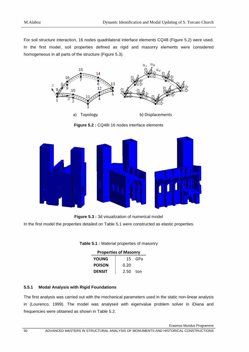
M.Alaboz Dynamic Identification and Modal Updating of S. Torcato Church
Erasmus Mundus Programme 50 ADVANCED MASTERS IN STRUCTURAL ANALYSIS OF MONUMENTS AND HISTORICAL CONSTRUCTIONS
For soil structure interaction, 16 nodes quadrilateral interface elements CQ48 (Figure 5.2) were used.
In the first model, soil properties defined as rigid and masonry elements were considered
homogeneous in all parts of the structure (Figure 5.3).
a) Topology b) Displacements
Figure 5.2 : CQ48I 16 nodes interface elements
Figure 5.3 : 3d visualization of numerical model
In the first model the properties detailed on Table 5.1 were constructed as elastic properties.
Table 5.1 : Material properties of masonry
Properties of Masonry
YOUNG 15 GPa POISON 0.20
DENSIT 2.50 ton 5.5.1 Modal Analysis with Rigid Foundations
The first analysis was carried out with the mechanical parameters used in the static non-linear analysis
in (Lourenco, 1999). The model was analysed with eigenvalue problem solver in iDiana and
frequencies were obtained as shown in Table 5.2.

Dynamic Identification and Modal Updating of S. Torcato Church M.Alaboz
Erasmus Mundus Programme ADVANCED MASTERS IN STRUCTURAL ANALYSIS OF MONUMENTS AND HISTORICAL CONSTRUCTIONS 51
Table 5.2 : Natural frequencies of the model with rigid foundations
MODE FREQUENCY [Hz]
1st 3.60
2nd 4.22
3rd 4.59
4th 4.74 The first four mode shapes are presented in Figure 5.4 . First mode is a translational mode in X
direction. Second mode is translational mode in Y direction. Third mode presents torsional mode when
the forth mode present opposite behaviour of towers (see Figure 5.4).
a) Mode 1 / 3.60 Hz b) Mode 2 / 4.22 Hz
c) Mode 3 / 4.59 Hz d) Mode 4 / 4.74
Figure 5.4 : Mode shapes presentation of numerical model
For modal comparison of numerical and experimental modes, only the first four modes were selected
because of accurate estimation in experimental analysis. Comparison of experimental numeric
analysis results exhibit high differences in both frequency and mode shape comparison (Table 5.3).
The average error is equal to 63% and the MAC values are lower than 0.84.

M.Alaboz Dynamic Identification and Modal Updating of S. Torcato Church
Erasmus Mundus Programme 52 ADVANCED MASTERS IN STRUCTURAL ANALYSIS OF MONUMENTS AND HISTORICAL CONSTRUCTIONS
Table 5.3 : Frequency and MAC value comparison of Model 1
Modes Experimental [Hz] FEM [Hz] Error [%] MAC
1st Transversal (Y ) 2.14 3.60 68.50 0.83 2nd Longitudinal (X) 2.63 4.22 60.66 0.85 3rd Torsional 2.85 4.59 60.71 0.12 4th Torsional 2.93 4.74 61.70 0.28
In Figure 5.5 a comparison of frequencies and MAC values are plotted. In the graph, distance of the
dots from the 45o line indicates the frequency difference when size of the dots indicates the ratio of
MAC values for each mode. When the dots are on the line, numerical model has the same frequencies
with experimental frequencies.
Figure 5.5 : Frequency versus scaled-MAC value comparison of Model 1
Mode shapes of numerical and experimental model are plotted below for visual comparison in Figure
5.6. First two translational modes are exhibit a consistence with experimental models when the third
and forth have no similarity even proved by low MAC values.
0.83
0.850.11
0.28
2
2.5
3
3.5
4
4.5
5
2 2.5 3 3.5 4 4.5 5
Expe
rimen
tal F
requ
enci
es
FEM Frequencies
MAC & Frequency Comparison

Dynamic Identification and Modal Updating of S. Torcato Church M.Alaboz
Erasmus Mundus Programme ADVANCED MASTERS IN STRUCTURAL ANALYSIS OF MONUMENTS AND HISTORICAL CONSTRUCTIONS 53
Experimental Model Finite Element Model
Mode 1
2.14 Hz
3.60 Hz
Mode 2
2.63 Hz
4.22 Hz
Mode 3
2.85 Hz
4.59 Hz
Mode 4
2.93 Hz
4.74 Hz
Figure 5.6 : Mode shape comparison of experimental and numerical models of Model 1
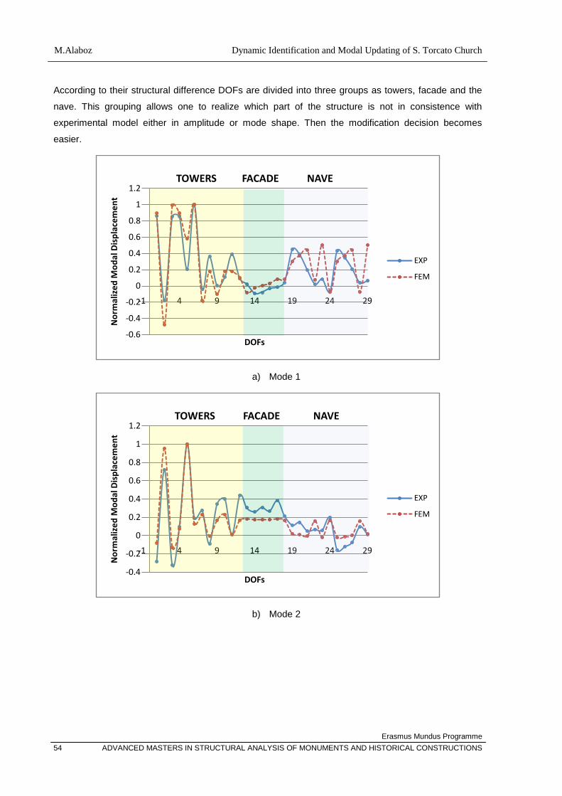
M.Alaboz Dynamic Identification and Modal Updating of S. Torcato Church
Erasmus Mundus Programme 54 ADVANCED MASTERS IN STRUCTURAL ANALYSIS OF MONUMENTS AND HISTORICAL CONSTRUCTIONS
According to their structural difference DOFs are divided into three groups as towers, facade and the
nave. This grouping allows one to realize which part of the structure is not in consistence with
experimental model either in amplitude or mode shape. Then the modification decision becomes
easier.
a) Mode 1
b) Mode 2
-0.6
-0.4
-0.2
0
0.2
0.4
0.6
0.8
1
1.2
-1 4 9 14 19 24 29
Nor
mal
ized
Mod
al D
ispl
acem
ent
DOFs
TOWERS FACADE NAVE
EXP
FEM
-0.4
-0.2
0
0.2
0.4
0.6
0.8
1
1.2
-1 4 9 14 19 24 29
Nor
mal
ized
Mod
al D
ispl
acem
ent
DOFs
TOWERS FACADE NAVE
EXP
FEM

Dynamic Identification and Modal Updating of S. Torcato Church M.Alaboz
Erasmus Mundus Programme ADVANCED MASTERS IN STRUCTURAL ANALYSIS OF MONUMENTS AND HISTORICAL CONSTRUCTIONS 55
c) Mode 3
d) Mode 4
Figure 5.7 : Normalized modal displacement comparisons of numerical and experimental model
-2
-1.5
-1
-0.5
0
0.5
1
1.5
-1 4 9 14 19 24 29
Nor
mal
ized
Mod
al D
ispl
acem
ent
DOFs
TOWERS FACADE NAVE
EXP
FEM
-10
-8
-6
-4
-2
0
2
4
6
8
10
-1 4 9 14 19 24 29
Nor
mal
ized
Mod
al D
ispl
acem
ent
DOFs
TOWERS FACADE NAVE
EXP
FEM

M.Alaboz Dynamic Identification and Modal Updating of S. Torcato Church
Erasmus Mundus Programme 56 ADVANCED MASTERS IN STRUCTURAL ANALYSIS OF MONUMENTS AND HISTORICAL CONSTRUCTIONS
5.5.1.1 Reduce of Elastic Modulus
Difference in frequencies between two models exhibits high values. Assuming that the geometric
definition of the model is correct, source of difference can be addressed to inappropriate estimation of
elastic modulus of masonry. Thus, the elastic modulus of masonry was decreased until the frequency
difference between models is reduced (Table 5.4 and Table 5.5).
Table 5.4 : Modified models and frequency comparison
Step 1 (10 GPa) Step 2 (8 GPa) Step 3 (6 GPa) Experimental
[Hz] Frequency
[Hz] Error [%]
Frequency [Hz]
Error [%]
Frequency [Hz]
Error [%]
2.14 2.94 37.51 2.63 23.01 2.27 6.17
2.63 3.44 31.05 3.08 17.33 2.66 1.33 2.85 3.74 31.09 3.34 17.07 2.9 1.65 2.93 3.86 31.83 3.45 17.83 2.99 2.12
Although, frequency error was reduced by changing the elasticity modulus of the model, mode shape
assurance MAC remains the same. Assuming that the geometrical definition of the church is reliable,
cracked regions should be introduced.
Table 5.5 : Frequency and MAC comparison of the modified model
Experimental Frequencies
[Hz]
Numerical Frequencies
[Hz]
Frequency Error [%] MAC
2.14 2.27 6.17 0.83 2.63 2.66 1.33 0.85 2.85 2.9 1.65 0.12 2.93 2.99 2.12 0.28
5.5.1.2 The Model with Crack Definition
Considering the previous analysis, the young modulus equal to 6 GPa was chosen for the masonry
material. To simulate the contribution of crack, the cracked regions were with a significant decrease of
the young modulus.
Cracked regions were defined according to previous crack pattern evaluation which was prepared with
the help of photogrammetric methods and visual inspections considering actual conditions of cracks.
For cracked region properties, elasticity modulus was decreased step by step until the contribution of
decrease has no effect on MAC values.

Dynamic Identification and Modal Updating of S. Torcato Church M.Alaboz
Erasmus Mundus Programme ADVANCED MASTERS IN STRUCTURAL ANALYSIS OF MONUMENTS AND HISTORICAL CONSTRUCTIONS 57
a) Crack pattern on facade and cracked region in numerical model
b) Crack pattern on north facade
c) Crack pattern on balcony
Figure 5.8 : Crack definition of numerical model

M.Alaboz Dynamic Identification and Modal Updating of S. Torcato Church
Erasmus Mundus Programme 58 ADVANCED MASTERS IN STRUCTURAL ANALYSIS OF MONUMENTS AND HISTORICAL CONSTRUCTIONS
Table 5.6 : Elastic properties of cracked region
Modifications Step 1 Step 2 Step 3 Step 4
Ecracked (GPa) 1 0.1 0.01 0.001 After crack definition with various elastic properties given in Table 5.6, frequency and MAC values
were calculated (see Table 5.7). As the elastic properties of cracked region were decreased relatively
to the elastic modulus of the masonry walls, the mode shapes are affected significantly. Nevertheless,
it is not possible to mention about an improvement. First step of the modification caused increment of
average MAC value (see Figure 5.9). However, the 2nd mode suffered from modification negatively
(Table 5.8).
Table 5.7 : Frequency and MAC values of modified models
Initial Model Step 1 Step 2 Step 3 Step 4 No crack Ecrack = 1 Gpa Ecrack = 0.1 Gpa Ecrack = 0.01 Gpa Ecrack = 0.001 Gpa EXP Freq. MAC Freq. MAC Freq. MAC Freq. MAC Freq. MAC 2.14 2.27 0.83 2.19 0.89 2.06 0.92 2.02 0.92 2.01 0.92 2.63 2.66 0.85 2.62 0.74 2.55 0.39 2.53 0.31 2.52 0.3 2.85 2.9 0.12 2.74 0.2 2.64 0.28 2.62 0.33 2.55 0.01 2.93 2.99 0.28 2.86 0.3 2.74 0.29 2.71 0.29 2.61 0.06
Figure 5.9 : Evaluation of modification by means of average frequency ratio and average MAC
In Figure 5.10 effect of crack definition is evaluated only for 3rd mode. The graph presents that until the
model in Step 4, MAC values are increasing.
Initial Model
Step 1
Step 2Step 3
Step 4
0.90.920.940.960.98
11.021.04
0.2 0.3 0.4 0.5 0.6
Aver
age
(f exp
/f FEM
)
Average (MAC)
Effect of crack definition

Dynamic Identification and Modal Updating of S. Torcato Church M.Alaboz
Erasmus Mundus Programme ADVANCED MASTERS IN STRUCTURAL ANALYSIS OF MONUMENTS AND HISTORICAL CONSTRUCTIONS 59
Figure 5.10 : Evaluation of modification by means of average frequency ratio and average MAC for Mode 3
In the last point, if we consider the base model and last modified model as Step 3, crack definition,
contributed to MAC values for Mode1, Mode3 and Mode4. However, the modification contributed to
the results with different ratios and even in 2nd mode contributed negatively.
Table 5.8 : Comparison of MAC values before and after crack definition
MAC
Modes Initial Model Step 3
1st 0.83 0.92
2nd 0.85 0.31
3rd 0.12 0.33
4th 0.28 0.29 Moreover, when mode shapes are compared, except first translational mode no coherence is
observed between models. Figure 5.11 shows the mode shapes for the model with crack definition
where the first mode shape numerical model is highly suitable with experimental but in second and
third modes, towers move independently. Forth mode is not affected by the modification. Most
effective contribution of crack definition is seen on 3rd mode. Nevertheless, mode shapes correlation
is not acceptable.
Other source of inaccuracy will be examined in further modifications, such as soil properties and effect
of missing transept part. It is sure that the crack pattern has a structural effect by forming discontinuity
but the way of simulating the crack cannot be achieved by reducing the elastic properties. Use of
interface elements which allow definition of different stiffness values in different directions or
evaluating the effect of crack under different conditions may be a solution.
Initial Model
Step 1Step 2
Step 3Step 4
0.880.9
0.920.940.960.98
11.021.04
0 0.1 0.2 0.3 0.4
Aver
age
(f exp
/f FEM
)
Average (MAC)
Effect of crack definition for Mode 3

M.Alaboz Dynamic Identification and Modal Updating of S. Torcato Church
Erasmus Mundus Programme 60 ADVANCED MASTERS IN STRUCTURAL ANALYSIS OF MONUMENTS AND HISTORICAL CONSTRUCTIONS
Experimental Model Finite Element Model
Mode 1
2.14 Hz
2.02 Hz
Mode 2
2.63 Hz
2.53 Hz
Mode 3
2.85 Hz
2.62 Hz
Mode 4
2.93 Hz
2.71 Hz
Figure 5.11 : Mode shape comparison of the model with crack definition

Dynamic Identification and Modal Updating of S. Torcato Church M.Alaboz
Erasmus Mundus Programme ADVANCED MASTERS IN STRUCTURAL ANALYSIS OF MONUMENTS AND HISTORICAL CONSTRUCTIONS 61
5.5.2 Modal Analysis with Elastic Foundations
After parametric modifications carried out in the model with rigid foundation, elastic soil properties
were introduced to better tune the experimental results while the other parameters were kept as it was
in the initial model (15 GPa elastic modulus of masonry). Soil properties are estimated by in situ
investigation (Lourenco & Ramos, 1999). According to vertical and horizontal stiffness parameters of
soil test, normal and transversal stiffness modulus were defined for 17 different regions of the
foundation (see Figure 5.12).
Figure 5.12 : Interface elements with different properties
Table 5.9 : Soil properties of the model with elastic foundation
Soil Properties [kPa]
Normal Transversal
Normal Transversal
INT 1 3900 1620
INT 10 98530 41050 INT 2 5120 2130
INT 11 84620 35260
INT 3 8430 3510
INT 12 14970 6240 INT 4 6140 2560
INT 13 18210 7590
INT 5 6240 2600
INT 14 42920 1788 INT 6 9360 3900
INT 15 32850 13690
INT 7 19760 8230
INT 16 67530 28140 INT 8 54990 22910
INT 17 56150 23400
INT 9 45650 19020

M.Alaboz Dynamic Identification and Modal Updating of S. Torcato Church
Erasmus Mundus Programme 62 ADVANCED MASTERS IN STRUCTURAL ANALYSIS OF MONUMENTS AND HISTORICAL CONSTRUCTIONS
Modal analysis results exhibit very low frequency values (see Table 5.10). By evaluating the mode
shapes (see Figure 5.13), it is observed that due to low elastic properties, the soil cannot simulate the
experimental results and cause rigid movement of the whole structure. However, the MAC values of
first two modes have higher values.
Table 5.10 : Modal analysis frequency estimations and MAC comparison with experimental model
Modes Experimental [Hz] FEM [Hz] Error [%] MAC
1st Transversal (Y ) 2.14 0.62 70.91 0.86
2nd Longitudinal (X) 2.63 0.79 69.94 0.71
3rd Torsional 2.85 1.23 56.89 0.07
4th Torsional 2.93 1.92 34.43 0.02
a) Mode 1 b) Mode 2
c) Mode 3 d) Mode 4
Figure 5.13 : Mode shapes of Model 2

Dynamic Identification and Modal Updating of S. Torcato Church M.Alaboz
Erasmus Mundus Programme ADVANCED MASTERS IN STRUCTURAL ANALYSIS OF MONUMENTS AND HISTORICAL CONSTRUCTIONS 63
5.5.2.1 Increase of Elastic Properties of Foundations
Due to low frequency and MAC value results of previous analysis, soil properties raised until the
contribution is null in MAC values (see Figure 5.14). When the elastic properties were increased, the
ratio of normal and shear stiffness in each interface element and the ratio between the zones were
kept constant. Elastic properties were multiplied by integer of 10 as given in Table 5.11.
Table 5.11 : Modification parameters of soil properties
Modification Parameters
Step 1 Step 2 Step 3
Multiplication Ratio 10 100 1000
Figure 5.14 : Effect of increasing the elastic properties of soill
Table 5.12 : Frequency and MAC value comparison of modified models
Initial Model Step 1 Step 2 Step 3 EXP Frequency MAC Frequency MAC Frequency MAC Frequency MAC 2.14 0.62 0.86 1.35 0.83 2.55 0.85 3.39 0.84 2.63 0.79 0.71 2.15 0.82 3.62 0.86 4.11 0.85 2.85 1.23 0.07 2.77 0.09 4.10 0.12 4.49 0.11 2.93 1.92 0.02 4.38 0.14 4.60 0.27 4.71 0.28
After increasing the soil properties, improvement of MAC values for each mode is observed except 1st
mode. However, the frequency difference is higher than acceptable range (Table 5.13).Thus the
elastic modulus of model was reduced to 10 GPa. Frequency and MAC comparison of modified model
is given in Table 5.13.
Initial Model
Step 1
Step 2
Step 3
0.5
0.7
0.9
1.1
1.3
1.5
0.2 0.4 0.6 0.8 1
Aver
age
(f exp
/f FEM
)
Average (MAC)
Effect of modification

M.Alaboz Dynamic Identification and Modal Updating of S. Torcato Church
Erasmus Mundus Programme 64 ADVANCED MASTERS IN STRUCTURAL ANALYSIS OF MONUMENTS AND HISTORICAL CONSTRUCTIONS
Table 5.13 : Frequency and mode shape comparison of modified model with experimental model
Modes Experimental [Hz] FEM [Hz] Error [%] MAC
1st Transversal (Y ) 2.138 2.25 5.24 0.85 2nd Longitudinal (X) 2.625 3.08 17.33 0.86 3rd Torsional 2.853 3.44 20.57 0.12 4th Torsional 2.928 3.78 29.10 0.27
Figure 5.15 : Experimental and numerical model comparison of the modified model
The contribution of the modification with respect to first model is given in Table 5.14. Relatively high
contribution is observed in the 3rd and 4th mode.
Table 5.14 : Contribution of modification in MAC for the model
MAC
Modes Initial Model Step 2 1st 0.86 0.85 2nd 0.71 0.86 3rd 0.07 0.12 4th 0.02 0.27
Mode shape comparison of experimental and numerical model is given in Figure 5.16. First and
second mode shapes are in high consistence as MAC values indicate. Although the MAC values of
third and forth mode shapes are very low, visual comparison of mode shapes exhibit that the general
behaviours are similar but the amplitudes are smaller and lack of torsional effects are lacking due to
improper modelling parameters.
0.850.86
0.120.27
1
1.5
2
2.5
3
3.5
4
4.5
5
1 1.5 2 2.5 3 3.5 4 4.5 5
Expe
rimen
tal F
requ
enci
es
FEM Frequencies
MAC & Frequency Comparison

Dynamic Identification and Modal Updating of S. Torcato Church M.Alaboz
Erasmus Mundus Programme ADVANCED MASTERS IN STRUCTURAL ANALYSIS OF MONUMENTS AND HISTORICAL CONSTRUCTIONS 65
Experimental Model Finite Element Model
Mode 1
2.14 Hz
2.25 Hz
Mode 2
2.63 Hz
3.08 Hz
Mode 3
2.85 Hz
3.44 Hz
Mode 4
2.93 Hz
3.78 Hz
Figure 5.16 : Mode shapes comparison of the model with experimental model

M.Alaboz Dynamic Identification and Modal Updating of S. Torcato Church
Erasmus Mundus Programme 66 ADVANCED MASTERS IN STRUCTURAL ANALYSIS OF MONUMENTS AND HISTORICAL CONSTRUCTIONS
5.5.2.2 Simulation of Transept
By increasing the soil properties, the coherence between two models improved. The other important
inadequacy in the model is the incomplete transept and apse part of the church. Due to lack of time,
missing part of the church couldn’t be constructed. Instead, interface elements were added. Interface
elements were defined at the edge of missing part where the walls of nave are intersecting with
transept, see Figure 5.17. Elastic modulus of the masonry was defined as 10 GPa.
Figure 5.17 : Interface elements defined at the edge of missing part
The free edge of the interface elements were constrained in three directions. Normal and shear
stiffness of the elements were defined with high elastic properties in order to start trials with a rigid
connection. Effect of the stiffness variation was studied one by one. The updating parameters are
given in Table 5.15 in kPa units.
Table 5.15 : Modification parameters of interface elements
Modifications
Normal [kPa] Transversal [kPa]
Step 1 1.00 E10 1.00 E10 Step 2 1.00 E8 1.00 E10 Step 3 1.00 E6 1.00 E10 Step 4 1.00 E4 1.00 E10 Step 5 1.00 E2 1.00 E10

Dynamic Identification and Modal Updating of S. Torcato Church M.Alaboz
Erasmus Mundus Programme ADVANCED MASTERS IN STRUCTURAL ANALYSIS OF MONUMENTS AND HISTORICAL CONSTRUCTIONS 67
Figure 5.18 : Effect of modification in frequency ratio and average MAC values of the model
Only the modification normal stiffness was reduced. As seen in Figure 2.1, when the connection is
more flexible in longitudinal direction of the nave, the frequency error is reduced and MAC values
increase. Due to significant drop in MAC value with the modifications in Step 5, the model in Step 4
was chosen for further modifications.
Table 5.16 : Frequency and MAC value of each modified model
Initial Model Step 1 Rigid
Step 2 100 GPa
Step 3 1 GPa
Step 4 10 MPa
Step 5 100 KPa
EXP Freq. MAC Freq. MAC Freq. MAC Freq. MAC Freq. MAC Freq. MAC 2.14 2.55 0.85 2.93 0.91 2.92 0.91 2.86 0.92 2.78 0.92 2.78 0.92 2.63 3.62 0.86 3.70 0.41 3.70 0.42 3.64 0.64 3.27 0.86 3.24 0.22 2.85 4.10 0.12 3.90 0.60 3.90 0.60 3.84 0.70 3.78 0.81 3.78 0.81 2.93 4.60 0.27 3.91 0.74 3.91 0.75 3.87 0.68 3.80 0.75 3.80 0.75
Table 5.17 : Frequency and mode shape comparison of modified model with experimental model
Modes Experimental [Hz] FEM [Hz] Error [%] MAC
1st Transversal (Y ) 2.138 2.78 30.03 0.92
2nd Longitudinal (X) 2.625 3.27 24.57 0.86
3rd Torisonal 2.853 3.78 32.49 0.81
4th Torsional 2.928 3.80 29.78 0.75
Initial ModelStep 1
Step 2Step 3
Step 4Step 5
1.25
1.3
1.35
1.4
1.45
0.4 0.5 0.6 0.7 0.8 0.9 1
Aver
age
(fexp
/fFEM
)
Average (MAC)
Effect of Modification

M.Alaboz Dynamic Identification and Modal Updating of S. Torcato Church
Erasmus Mundus Programme 68 ADVANCED MASTERS IN STRUCTURAL ANALYSIS OF MONUMENTS AND HISTORICAL CONSTRUCTIONS
Figure 5.19 : Frequency versus MAC value presentation of modified model in Step 4
When the base model before modifications and the last model compared, high improvement of 3rd
and 4th mode is obvious even though minor improvement is seen in 1st mode (see Table 5.18).
Table 5.18 : Contribution of modifications in MAC values for the model
MAC
Modes Initial Model Step 4
1st 0.85 0.92
2nd 0.86 0.86
3rd 0.12 0.81
4th 0.27 0.75 When the mode shapes given in Figure 5.20 are examined, similar movement of DOFs is observed.
Difference between the experimental and numerical model can be related with magnitude differences
and some local differences of measured DOFs. In the forth mode shape opposite movements of the
towers present consistency with the experimental mode, but it is seen that the towers in experimental
mode have more torsional effect.
0.92
0.86
0.81
0.75
2
2.5
3
2 2.5 3
Expe
rimen
tal F
requ
enci
es
FEM Frequencies
MAC & Frequency Comparison

Dynamic Identification and Modal Updating of S. Torcato Church M.Alaboz
Erasmus Mundus Programme ADVANCED MASTERS IN STRUCTURAL ANALYSIS OF MONUMENTS AND HISTORICAL CONSTRUCTIONS 69
Experimental Model Finite Element Model
Mode 1
2.14 Hz
2.78 Hz
Mode 2
2.63 Hz
3.27 Hz
Mode 3
2.85 Hz
3.78 Hz
Mode 4
2.93 Hz
3.80 Hz
Figure 5.20 : Mode shapes comparison of the model in Step 4 with the experimental model

M.Alaboz Dynamic Identification and Modal Updating of S. Torcato Church
Erasmus Mundus Programme 70 ADVANCED MASTERS IN STRUCTURAL ANALYSIS OF MONUMENTS AND HISTORICAL CONSTRUCTIONS
Interface elements which are defined in order to simulate the missing part of the structure, have two
stiffness properties for normal and shear directions. Effect of stiffness change in normal direction was
studied in previously. In this step, effect of the stiffness property in shear plane will be studied.
The model that exhibits best performance in previous modifications is chosen as the base model.
When keeping the stiffness property in normal direction constant, shear stiffness was modified as
given in Table 5.19.
Table 5.19 : Modification parameters of interface elements
Normal Stiffness
[GPa] Shear Stiffness
[GPa] Initial Model 1.00 E4 1.00 E10
Step 1 1.00 E4 1.00 E8 Step 2 1.00 E4 1.00 E7 Step 3 1.00 E4 1.00 E6
In Figure 5.21 effect of reducing the shear stiffness shows that improving the average MAC value in a
very narrow range and also the contribution for frequency ratio is very low. However as the best
performing model in Step 2 is chosen as the base model for parametric decision. In previous steps
contribution of modifications were examined linearly but this method avoid studying the combined
effect of different parameter changes. Thus, a non linear relation of chosen parameters will be studied
in further sections.
Figure 5.21 : Effect of modification in frequency ratio and average MAC values of the model
Initial Model
Step 2
Step 1
Step 3
1.28
1.282
1.284
1.286
1.288
1.29
1.292
1.294
0.7 0.75 0.8 0.85 0.9 0.95 1
Aver
aha
(fexp
/fFEM
)
Average (MAC)
Effect of Modification

Dynamic Identification and Modal Updating of S. Torcato Church M.Alaboz
Erasmus Mundus Programme ADVANCED MASTERS IN STRUCTURAL ANALYSIS OF MONUMENTS AND HISTORICAL CONSTRUCTIONS 71
As can be seen in Table 5.20 mode 2 and mode 3 were suffered from a minor improvement in MAC
values but the frequency difference is still higher. In order to reduce the frequency difference non
linear relation of modifications should be studied. Comparison of the modified model with experimental
model is given in Table 5.21 and the contribution of modifications in
Table 5.22.
Table 5.20 : Frequency and MAC value of each modified model
Initial Model Step 1
100 GPa Step 2 10 GPa
Step 3 10 GPa
EXP Freq. MAC Freq. MAC Freq. MAC Freq. MAC 2.14 2.78 0.92 2.78 0.92 2.77 0.92 2.75 0.93 2.63 3.27 0.86 3.26 0.86 3.26 0.86 3.21 0.85 2.85 3.78 0.81 3.78 0.81 3.78 0.84 3.77 0.61 2.93 3.80 0.75 3.80 0.75 3.80 0.78 3.79 0.48
Table 5.21 : Frequency and mode shape comparison of modified model with experimental model
Modes Experimental [Hz] FEM [Hz] Error [%] MAC
1st Transversal (Y ) 2.14 2.77 29.56 0.92
2nd Longitudinal (X) 2.63 3.26 24.19 0.86
3rd Torsional 2.85 3.78 32.49 0.84
4th Torsional 2.93 3.80 29.78 0.78
Table 5.22 : MAC value contribution of modifications for the model in Step 2
MAC
Modes Initial Model Step 2 1st 0.92 0.92 2nd 0.86 0.86 3rd 0.81 0.84 4th 0.75 0.78

M.Alaboz Dynamic Identification and Modal Updating of S. Torcato Church
Erasmus Mundus Programme 72 ADVANCED MASTERS IN STRUCTURAL ANALYSIS OF MONUMENTS AND HISTORICAL CONSTRUCTIONS
Figure 5.22 : Frequency versus MAC value presentation of the modified model
As it can be seen in Table 5.22 and presented in Figure 5.22, MAC values are increased by the
modifications and frequency difference is reduced by giving lower elasticity modulus for masonry.
However the frequency error is high with around 30%.
When the mode shapes are examined, as it is proved by reasonable MAC values, they present high
consistency with the experimental model. Improper correlation in previous analysis of third and forth
mode, gives similar responses.
Within consideration of frequency and MAC value performance, the model in Step 2 was chosen.
Although the effect of modification parameters was studied, to find the combined effect and
optimization, Douglas-Reid Method will be carried.
0.93
0.860.84
0.78
2
2.5
3
2 2.5 3
Expe
rimen
tal F
requ
enci
es
FEM Frequencies
MAC & Frequency Comparison

Dynamic Identification and Modal Updating of S. Torcato Church M.Alaboz
Erasmus Mundus Programme ADVANCED MASTERS IN STRUCTURAL ANALYSIS OF MONUMENTS AND HISTORICAL CONSTRUCTIONS 73
Experimental Model Finite Element Model
Mode 1
2.14 Hz
2.77 Hz
Mode 2
2.63 Hz
3.26 Hz
Mode 3
2.85 Hz
3.78 Hz
Mode 4
2.93 Hz
3.80 Hz
Figure 5.23 : Mode shape comparison of the model in Step 2 with experimental model

M.Alaboz Dynamic Identification and Modal Updating of S. Torcato Church
Erasmus Mundus Programme 74 ADVANCED MASTERS IN STRUCTURAL ANALYSIS OF MONUMENTS AND HISTORICAL CONSTRUCTIONS
5.5.3 Robust Modal Updating of Selected Model
The model in with the last modifications is chosen as the best performed model for frequency
optimization (Table 5.23). In order to minimize the residuals and study the contribution of each
updating parameter the Douglas-Reid method was applied to this model.
Table 5.23 : Initial Properties of the modified model before optimization
Properties of Masonry
Soil Properties [kPa] Normal Shear Normal Shear
Stiffness Stiffness Stiffness Stiffness YOUNG 10 GPa INT 1 390000 162000 INT 10 9853000 4105000 POISON 0.2 INT 2 512000 213000 INT 11 8462000 3526000 DENSIT 2.5 ton INT 3 843000 351000 INT 12 1497000 624000
Interface Elements INT 4 614000 256000 INT 13 1821000 759000 Normal Stiffness Shear Stiffness INT 5 624000 260000 INT 14 4292000 178800 1 MPa 10 GPa INT 6 936000 390000 INT 15 3285000 1369000
INT 7 1976000 823000 INT 16 6753000 2814000
INT 8 5499000 2291000 INT 17 5615000 2340000
INT 9 4565000 1902000
For Douglas-Reid frequency tuning, variables defined for base, lower and upper cases are given in
Table 5.24. Those variables were used to obtain equations presented in Section 5.4 .Upper and lower
bound ranges were defined according to the previous analysis. When the bound parameters of the soil
were defined, INT 1 was chosen as the base value. According to modification of this parameter, the
other soil properties modified by keeping the ratio of elements constant.
Table 5.24 : Upper and lower bound properties variables
Updating Variables Name
Base (b)
Lower (low)
Upper (upr) Unit
1 Emasonry 10 4 15 GPa 2 Esoil 0.39 0.039 3.9 GPa 3 E-IntNormal Stiffness 0.01 0.001 0.1 GPa 4 E-IntShear Stiffness 10 1 100 GPa
Each model with properties listed above was solved; the frequencies and MAC values were obtained
as given in Table 5.25. “F” values represent the frequencies and “M” values MAC results for different
combination of the base model.

Dynamic Identification and Modal Updating of S. Torcato Church M.Alaboz
Erasmus Mundus Programme ADVANCED MASTERS IN STRUCTURAL ANALYSIS OF MONUMENTS AND HISTORICAL CONSTRUCTIONS 75
Table 5.25 : Frequencies of the models for each variable [Hz]
Combinations F1 F2 F3 F4 M1 M2 M3 M4
(1b,2b,3b,4b) 2.775 3.255 3.783 3.795 0.92 0.86 0.84 0.78
(1low,2b,3b,4b) 1.907 2.167 2.419 2.440 0.91 0.85 0.72 0.60
(1upr,2b,3b,4b) 3.234 3.858 4.593 4.612 0.92 0.85 0.62 0.49
(1b,2low,3b,4b) 2.772 3.235 3.782 3.794 0.92 0.85 0.85 0.79
(1b,2upr,3b,4b) 3.201 3.501 3.856 3.915 0.90 0.85 0.71 0.58
(1b,2b,3low,4b) 2.772 3.234 3.782 3.793 0.92 0.85 0.85 0.78
(1b,2b,3upr,4b) 2.793 3.396 3.791 3.810 0.92 0.86 0.79 0.73
(1b,2b,3b,4low) 2.751 3.215 3.773 3.785 0.93 0.85 0.60 0.48
(1b,2b,3b,4upr) 2.779 3.264 3.784 3.799 0.92 0.86 0.81 0.75
Non linear solutions of the equations were calculated by the numerical solver software GAMS (GAMS,
2002) gave the estimation of optimum parameters presented in Table 5.26.
Table 5.26 : Non linear estimation of optimum modification parameters
Variables Name Optimum Unit
1st Emasonry 5.642 GPa 2nd Esoil 0.629 GPa 3rd E-IntNormal Stiffness 0.046 GPa 4th E-IntShear Stiffness 21.591 GPa
When the model is solved with optimum parameters, frequency difference of the models was reduced
significantly but decrease of MAC values was observed.
Table 5.27 : Comparison of the model modified with Douglas-Reid
Modes Experimental [Hz] FEM [Hz] Error [%] MAC
1st Transversal (Y ) 2.14 2.29 7.11 0.91
2nd Longitudinal (X) 2.63 2.63 0.19 0.85
3rd Torsional 2.85 2.88 0.95 0.72
4th Torsional 2.93 2.91 0.61 0.60

M.Alaboz Dynamic Identification and Modal Updating of S. Torcato Church
Erasmus Mundus Programme 76 ADVANCED MASTERS IN STRUCTURAL ANALYSIS OF MONUMENTS AND HISTORICAL CONSTRUCTIONS
Figure 5.24 : Frequency versus MAC value presentation of the model modified with Douglas-Reid method
Procedure was repeated with the same combinations but only changing the weightening factor of the
MAC error which takes place in objective function. When the weightening factor of the frequencies are
“1”, MAC errors were multiplied by “1.2” in order to increase MAC sensitivity of the method.
By changing the weightening factor of MAC, a reasonable increase is observed especially in third and
forth mode. Although the frequency error for second and third mode increase, frequency error
distribution is better than the previous model (see Table 5.28).
Table 5.28 : Frequency and MAC value comparison of the modified model
Modes Experimental [Hz] FEM [Hz] Error [%] MAC
1st Transversal (Y ) 2.14 2.14 0.09 0.92
2nd Longitudinal (X) 2.63 2.55 2.86 0.86
3rd Torsional 2.85 2.93 2.70 0.83
4th Torsional 2.93 2.94 0.41 0.77
0.93
0.860.66
0.51
2
2.5
3
2 2.5 3Expe
rimen
tal F
requ
enci
es
FEM Frequencies
MAC & Frequency Comparison

Dynamic Identification and Modal Updating of S. Torcato Church M.Alaboz
Erasmus Mundus Programme ADVANCED MASTERS IN STRUCTURAL ANALYSIS OF MONUMENTS AND HISTORICAL CONSTRUCTIONS 77
Experimental Model Finite Element Model
Mode 1
2.14 Hz
2.14 Hz
Mode 2
2.63 Hz
2.55 Hz
Mode 3
2.85 Hz
2.93 Hz
Mode 4
2.93 Hz
2.94 Hz
Figure 5.25 : Mode shapes comparison of the modified model

M.Alaboz Dynamic Identification and Modal Updating of S. Torcato Church
Erasmus Mundus Programme 78 ADVANCED MASTERS IN STRUCTURAL ANALYSIS OF MONUMENTS AND HISTORICAL CONSTRUCTIONS
The mode shapes of the modified model exhibit high consistence with experimental mode shapes. In
first and second mode shapes which are translational modes, no significant difference is observed
between the models. The third mode shape of the numerical model present similar behaviour with
experimental model, but when the north tower is examined, it is seen that the torsional effect is higher
than the numerical model. Forth mode shape of the towers also exhibit similar behaviour but the
reason of having low MAC values can be related with amplitudes of DOF’s and due to lack of damage
simulation on the facade, negative contribution of this part.
a) Mode 1
b) Mode 2
-0.4
-0.2
0
0.2
0.4
0.6
0.8
1
1.2
-1 4 9 14 19 24 29
Nor
mal
ized
Mod
al D
ispl
acem
ent
DOFs
TOWERS FACADE NAVE
EXP
FEM
-0.4
-0.2
0
0.2
0.4
0.6
0.8
1
1.2
-1 4 9 14 19 24 29
Nor
mal
ized
Mod
al D
ispl
acem
ent
DOFs
TOWERS FACADE NAVE
EXP
FEM

Dynamic Identification and Modal Updating of S. Torcato Church M.Alaboz
Erasmus Mundus Programme ADVANCED MASTERS IN STRUCTURAL ANALYSIS OF MONUMENTS AND HISTORICAL CONSTRUCTIONS 79
c) Mode 3
d) Mode 4
Figure 5.26 : Normalized Modal displacement comparison of each DOF for mode shapes
Comparison of normalized mode displacements of each DOF can be seen in Figure 5.26. As it can be
seen in the graphs most synchronised behaviour of the modal shapes are observed in towers. The
source of the difference is mostly the magnitude. Although minor differences are observed, DOFs in
the nave follow the mode shape mostly in first two modes. DOFs in the facade where is the most
damaged part of the structure, have irregularities. When the DOFs of numerical model follow a linear
way, due to significant damages irregular movements are observed in the experimental model.
-1.5
-1
-0.5
0
0.5
1
1.5
-1 4 9 14 19 24 29
Nor
mal
ized
Mod
al D
ispl
acem
ent
DOFs
TOWERS FACADE NAVE
EXP
FEM
-1.5
-1
-0.5
0
0.5
1
1.5
-1 4 9 14 19 24 29
Nor
mal
ized
Mod
al D
ispl
acem
ent
DOFs
TOWERS FACADE NAVE
EXP
FEM

M.Alaboz Dynamic Identification and Modal Updating of S. Torcato Church
Erasmus Mundus Programme 80 ADVANCED MASTERS IN STRUCTURAL ANALYSIS OF MONUMENTS AND HISTORICAL CONSTRUCTIONS
After robust optimization processes, the effect of the cracked region was studied. Cracked region was
simulated by decreasing the elastic modulus of damaged part with the properties given in
Table 5.29.
Table 5.29 : Modification parameters of cracked region
Modifications Ecrack
Step 1 5 GPa Step 2 4 GPa Step 3 3 GPa Step 4 2 GPa Step 5 1 GPa
Figure 5.27 : Effect of crack definition in frequency error versus average MAC
As it can be seen in Figure 5.27, by decreasing the elastic properties of cracked region, frequency
error increase and MAC values decrease. Due to negative contribution of crack definition, initial model
which was tuned with Douglas-Reid method is chosen as ultimate model.
In order to evaluate the final model with a different criteria, NMD values are also calculated (Table
5.30 and Table 5.31).
Table 5.30 : NMD values of the modified model
MAC NMD Mode 1 0.92 0.29 Mode 2 0.86 0.41 Mode 3 0.83 0.46 Mode 4 0.77 0.54

Dynamic Identification and Modal Updating of S. Torcato Church M.Alaboz
Erasmus Mundus Programme ADVANCED MASTERS IN STRUCTURAL ANALYSIS OF MONUMENTS AND HISTORICAL CONSTRUCTIONS 81
Although by means of frequency and MAC value results, final updated model gives satisfactory
results, the NMD values which are more sensitive for differences values present high values.
According to the expression, the more values of NMD increase the difference of the mode shapes
increase. Thus except the first mode shape of the updated model, differences between the mode
shapes are very high (see Table 5.31).
Figure 5.28 : Initial model without modifications and the effect of each modification step
In Figure 5.28, starting from the initial model, effect of all the modifications are plotted by means of
frequency ratio and MAC values. The final point presents a high contribution of the modifications
relative to the starting point. However, the evaluation of results and still being far from the target point
which is desired to be “1” for MAC values and “1” for frequency ratios indicates need of other
modifications. Possible reasons of low consistence and recommendations for the better model will be
discussed in conclusion.
Target Point
Initial Model
Increase of Soil Properties
Douglas-Reid Optimization
Definition of Transept
0
0.2
0.4
0.6
0.8
1
1.2
1.4
0.2 0.3 0.4 0.5 0.6 0.7 0.8 0.9 1
Aver
age
(fexp
/fFEM
)
Average (MAC)
Effect of Modifications

M.Alaboz Dynamic Identification and Modal Updating of S. Torcato Church
Erasmus Mundus Programme 82 ADVANCED MASTERS IN STRUCTURAL ANALYSIS OF MONUMENTS AND HISTORICAL CONSTRUCTIONS
6 CONCLUSIONS AND RECOMMENDATIONS
Experimental identification campaign on San Torcato Church was started on 29 April 2009 and
completed in 26 May with several measurements. Firstly, dynamic identification of the entire structure
was carried out. In the experiments ambient vibrations were recorded with 10 piezoelectric
accelerometers and additionally hammer excitement test, soil measurements in three axes were
taken. Data acquisition system was set on the main nave in a point where the electric supply is nearby
and the accesses to measurement points are convenient. Records were pre processed in the field to
check the quality of the measurements.
The data collected in the field was checked for their measurement quality and processed with different
methods for each setup separately and all setups combined. Due to low excitement of the structure
only first four global modes of the structure was accurately identified. The frequencies obtained by the
experimental techniques were consistent with preliminary dynamic identification tests.
6.1 Experimental Testing
Beside the benefits of the method, great care should be taken in field test to avoid data loss. During
the experiments, some expected and unexpected problems were faced. Those problems are listed
below to give recommendations;
• Before starting a dynamic test on a structure, a numerical model should be constructed in
order to estimate frequency values and mode shapes. This numerical model will lead the
researcher to decide the type of accelerometer to use, place of the DOFs to be measured and
even to compare the first experimental results.
• Test planning should be decided following a site trip in order to see the difficulties for fixing the
accelerometers and to check if the access provided. Considering the length of the cables and
the number of the connections used in a line, the distance between DOFs should be minimum.
Although there is no limitation for the cables length and the number of connections, it should
be kept in mind that the frequently encountered problems of having noise but no signal are
mostly originated from connections.
• When the number of channels increase and the distance between DOFs and DAQ is high,
cables have to be organized well. To avoid misconnections of the cables, perpetual numbering
of cables is advised and the coordination between the workers in the field should be clear and
precise.
• Each measurement should be supported with notes of the environmental conditions and
events likely to occur during the measurements. If possible the temperature, humidity and
wind speed values should be recorded.
• Supports of the accelerometers should be checked properly to avoid undesired noise. Due to
having different sensitivity values of each accelerometer, all of them should be marked and

Dynamic Identification and Modal Updating of S. Torcato Church M.Alaboz
Erasmus Mundus Programme ADVANCED MASTERS IN STRUCTURAL ANALYSIS OF MONUMENTS AND HISTORICAL CONSTRUCTIONS 83
care should be taken to state which accelerometer is connected to which channel, in which
DOF and direction.
6.2 Modal Updating
The numerical model which was previously constructed was modified by using manual modification
techniques and robust optimization algorithms. Due to lack of time, missing part of the model couldn’t
be constructed. Modifications were carried out on homogeneous elastic properties of masonry, elastic
soil properties and stiffness parameters of the interface elements which were added to model in order
to simulate the missing part of the model. Damages observed on the structure were simulated by
giving low elastic properties in cracked regions. Nevertheless, no positive contribution was realized.
Although the initial models are suffered an improvement, to increase the performance of the model
following statements should be considered;
• Due to significant damage occurrence on the main facade and certain inclination of towers,
only half of the structure was modelled. However, to better simulate the existing situation,
transept and apse part of the structure and one story additional spaces beside the nave
should be added to the model.
• Considering the width of the cracks observed on the main facade and on the balcony, it is
expected that the dynamic response of the structure is affected. To better simulate the cracks,
the use of interface elements is advisable. Moreover, the architectural details were not
considered in balcony part where there are arches supported with slender stone columns.
Increase of architectural details and a better crack definition can lead to a more realistic
model.
• In this analysis, openings on the towers, the bells on the north tower and the roofs were not
modelled. The timber roof of the main nave should have a significant effect on dynamic
behaviour, mainly with its lateral stiffness effect on the structure. Modelling those elements
should improve the realistic dynamic response of the numerical model.
• Masonry material is defined homogeneously in the whole model, but as it was stressed before,
due to construction phases, different materials were used in the structure. Those material
changes and their support conditions should be also introduced to improve the results.

M.Alaboz Dynamic Identification and Modal Updating of S. Torcato Church
Erasmus Mundus Programme 84 ADVANCED MASTERS IN STRUCTURAL ANALYSIS OF MONUMENTS AND HISTORICAL CONSTRUCTIONS
7 REFERENCES
Chopra A. (2001). Dynamics Of Structures,Theory and Applications to Earthquake Engineering (2nd
Edition b.), New Jersey Prentice-Hall.
Ewins D. (1984). Modal Testing:Theory and Practise . Chichester: Research Studies Press LTD.
Friswell M. I., Mottershead J.E., Ahmadian H. (2009). Finite element model updating using
experimental test data:parametrization and regularization. Philosophical Transactions of The Royal
Society A , 168-186.
Allemang J. R. (2003). The Modal Assurance Criterion – Twenty Years of Use and Abuse. Sound and
Vibration , 14-21.
Merluzzi N., Lee H., Suganya K., Wan I.M. (2007). Integrated project Report of St. Torcato Church.
Guimaraés, Portugal: University of Minho.
Mottershead J. E., Friswell, M. I. (1993). Modal Updating in Structural Dynamics : A Survey. Journal of
Sound and Vibration , 347-375.
Peeters B., De Roeck G. (2001). Stochastic System Identification for Operational Modal Analysis:A
Review. Journal of Dynamic Systems, Measurement, and Control , 659-667.
Ramos L.F., Aguilar R. (2007). Dynamic Identification of St. Torcato’s Church : Preliminary Tests.
Guimaraés, Portugal: University of Minho.
Ramos L. F. (2007). Damage Identification on Masonry Structures Based on Vibration Signatures.
Guimaraés: Universidade do Minho.
Clough R.W., Penzien J. (1995). Dynamics of Structures. Berkeley: Computers & Structures, Inc.
Rodrigues J., Brincker. R., Andersen P. (2001). Improvement of Frequency Domain Output-Only
Modal Identification from the Application of the Random Decrement Technique.
Brincker R., Zhang L, Andersen P. (2000). Output-only Modal Analysis by Frequency Domain
Decomposition. Proceedings of ISMA25 Volume 2

Dynamic Identification and Modal Updating of S. Torcato Church M.Alaboz
Erasmus Mundus Programme ADVANCED MASTERS IN STRUCTURAL ANALYSIS OF MONUMENTS AND HISTORICAL CONSTRUCTIONS 85
DOUGLAS, B.M., REID, W.H. (1982). Dynamic tests and system identification of bridges, Journal
Struct. Div., ASCE,108, 2295-2312
TNO (2008), “DIsplacement method ANAlyser”, version 9.3, Cd-Rom, Netherland. GAMS, D.C. (2002); “The General Algebraic Modeling System”, Cd-Rom, USA. ARTeMIS (2009), “Structural Vibration Solutions A/S”, Cd-Rom, Denmark MATLAB (2007), “The Language of Technical Computing” , Cd-Rom, USA