Multivariate source prelocalization (MSP): Use of functionally informed basis functions for better...

www.elsevier.com/locate/ynimg

NeuroImage 26 (2005) 356–373

Multivariate source prelocalization (MSP): Use of functionally

informed basis functions for better conditioning the

MEG inverse problem

J. Mattout,a,c,d,e,* M. Pelegrini-Issac,b,e L. Garnero,c,e and H. Benalid,e

aWellcome Department of Imaging Neuroscience, London, UKbINSERM U483, Paris, FrancecCNRS UPR640, Paris, FrancedINSERM U494, Paris, FranceeIFR49, Paris, France

Received 16 April 2004; revised 29 October 2004; accepted 21 January 2005

Available online 16 March 2005

Spatially characterizing and quantifying the brain electromagnetic

response using MEG/EEG data still remains a critical issue since it

requires solving an ill-posed inverse problem that does not admit a

unique solution. To overcome this lack of uniqueness, inverse methods

have to introduce prior information about the solution. Most existing

approaches are directly based upon extrinsic anatomical and functional

priors and usually attempt at simultaneously localizing and quantifying

brain activity. By contrast, this paper deals with a preprocessing tool

which aims at better conditioning the source reconstruction process, by

relying only upon intrinsic knowledge (a forward model and the MEG/

EEG data itself) and focusing on the key issue of localization. Based on a

discrete and realistic anatomical description of the cortex, we first define

functionally Informed Basis Functions (fIBF) that are subject specific.

We then propose a multivariate method which exploits these fIBF to

calculate a probability-like coefficient of activation associated with each

dipolar source of the model. This estimated distribution of activation

coefficients may then be used as an intrinsic functional prior, either by

taking these quantities into account in a subsequent inverse method, or

by thresholding the set of probabilities in order to reduce the dimension

of the solution space. These two ways of constraining the source

reconstruction process may naturally be coupled. We successively des-

cribe the proposedMultivariate Source Prelocalization (MSP) approach

and illustrate its performance on both simulated and real MEG data.

Finally, the better conditioning induced by theMSP process in a classical

regularization scheme is extensively and quantitatively evaluated.

D 2005 Elsevier Inc. All rights reserved.

Keywords: MEG/EEG; Inverse problem; Regularization; Better condition-

ing; Functionally Informed Basis Functions (fIBF); Activation probability;

Multivariate Source Prelocalization (MSP)

1053-8119/$ - see front matter D 2005 Elsevier Inc. All rights reserved.

doi:10.1016/j.neuroimage.2005.01.026

* Corresponding author. Wellcome Department of Imaging Neuroscience,

12 Queen Square, WC1N 3BG London, UK. Fax: +44 207 807 1420.

E-mail address: [email protected] (J. Mattout).

Available online on ScienceDirect (www.sciencedirect.com).

Introduction

As main tools for mapping the cognitive functions of the human

brain, functional imaging has a twofold objective: localizing the

populations of neurons involved in cognitive or behavioral tasks

and characterizing the temporal dynamics between those popula-

tions. To this end, functional imaging techniques should con-

sequently and ideally offer optimal spatial and temporal

resolutions. Quantifying those resolutions is still an open issue.

Nevertheless, the spatial and temporal resolutions should reach the

order of 1 mm and 1 ms, respectively, to adequately describe the

underlying physiological phenomenon of brain activity.

Current functional imaging techniques, Positron Emission

Tomography (PET), Single Photon Emission Computed Tomog-

raphy (SPECT) and functional Magnetic Resonance Imaging

(fMRI) present rather a good and even an excellent spatial

resolution (~5 mm, ~1 cm and ~3 mm, respectively (Hoffman

et al., 1979; Moonen and Bandettini, 1999). However, they all fail

to offer a high enough temporal precision. fMRI offers the best

trade-off, acquiring the signal of the whole brain in about 1 s, but

remains limited by the hemodynamic delay.

Because of their excellent temporal resolution (of the order of 1

ms, which roughly corresponds to the sampling rate), electro-

encephalography (EEG) and magnetoencephalography (MEG)

provide the most relevant data for studying the temporal dynamics

of brain activity. Unfortunately, substantial difficulties lie in the

inverse problem one has to solve in order to localize the

electromagnetic sources that induce both EEG and MEG scalp

recordings. This so-called ill-posed mathematical issue is indeed

largely ill conditioned due to the non-uniqueness of the solution

and numerical instability. The solution space (the brain) is much

larger than the data space (up to about 128 EEG electrodes or 250

MEG sensors) and furthermore, an infinite number of different

source arrangements can lead to the same measurements (Malmi-

vuo and Plonsey, 1995).

J. Mattout et al. / NeuroImage 26 (2005) 356–373 357

Except for the more realistic but also more complicated

multipolar approach (Mosher et al., 1999b; Nolte and Curio,

2000), current dipoles constitute the most appropriate and widely

used electromagnetic source model, whatever the inverse method

chosen among the two groups we distinguish hereafter. We refer

the reader to Baillet et al. (2001) for a thorough review of inverse

methods in MEG/EEG.

First approaches, called bdipole fitQ methods, consist of finding

very few equivalent current dipoles (ECD) whose contributions fit

the data best (Koles, 1998; Mosher et al., 1992; Scherg and von

Cramon, 1986). The position, orientation and amplitude of each

dipole remain to be determined by the algorithm but the number of

sources to be fitted has to be set a priori by the user. This strong

constraint and the lack of a precise anatomical description of the

solution space may yield unrealistic estimated sources.

By contrast, the second group of methods relies on the

distribution of numerous dipoles at fixed positions within the head

volume (Dale and Sereno, 1993). This so-called distributed source

model is suitable for inverse problem regularization and enables

the introduction of anatomical, physiological and functional priors

(Baillet and Garnero, 1997; Dale et al., 2000; Liu et al., 1998).

However, due to the large amount of dipoles necessary for

describing the solution space (~10,000 for the whole cortex strip),

the inverse problem usually remains highly ill conditioned.

Another limitation arises from the size of the initial solution space

the algorithms are able to account for (up to a few thousands

sources only). Moreover, these methods attempt to simultaneously

localize (by focusing on a few dipoles that are expected to be

activated) and quantify (by estimating the amplitude of these

dipoles) the neuronal activation, hence still retaining too many

parameters at the expense of better conditioning the problem.

Since ill-posedness is due to spatial indeterminacy, separating

the localization issue from the source amplitude estimation could

facilitate the source reconstruction. Indeed, ideally, once the

position and the orientation of the few sources that produced

some given MEG or EEG measures are established, estimating the

amplitude of these sources then only requires the inversion of a

well-determined system.

In this paper, we propose an original approach that focuses

exclusively on the localization of the activated brain areas. Within

the framework of distributed source modeling, our Multivariate

Source Prelocalization (MSP) method exploits what neuropsychol-

ogists call normalized scalp distributions, topologies or maps of

event-related fields or potentials (McCarthy and Wood, 1985).

Working on both the measured signals and the putative contribu-

tions of each cortical area to these data, MSP dissociates the classic

reconstruction problem into two parts: the estimation of the source

spatial distribution and the estimation of the source amplitudes.

Most importantly, MSP only deals with this first and crucial issue

(hence Prelocalization). Through the use of functionally Informed

Basis Functions (fIBF), MSP allows one to uniquely summarize

the putative contributions of the whole brain and to quantitatively

compare them with the measured scalp topologies in a multivariate

fashion. This yields an estimation of the cortical spatial support of

the ongoing activity and such information can be used for then

constraining any inverse method which classically aims at

estimating the intensity of each brain region. We show how some

quantitative information can be derived from the multivariate

comparison between the normalized measured maps and the

normalized scalp contribution of each putative activated source

of the distributed model. In an empirical Bayes-like logic, this

functional information can then be introduced as prior constraints

for better conditioning the source estimation.

The three steps of the proposed procedure are described in the

following section. In the next section, we then detail both the

numerical simulations we conducted and the real data set we

analyzed to evaluate the performance of the MSP approach in

terms of source prelocalization and as a regularization prior within

a Weighted Minimum Norm (WMN) criterion. Results are

presented in the further next section and finally discussed together

with the method in the last section.

Theory

Notations

Let us consider a t sample-wide window of MEG or EEG

measurements acquired on n sensors. When leaning on a

distributed source model involving p dipoles with fixed position

and orientation (Dale and Sereno, 1993), solving the MEG/EEG

inverse problem amounts to estimate the dipole amplitudes that

satisfy the linear matrix equation

M ¼ GJ þ E; ð1Þ

where M is the n � t data matrix, G is the n � p forward operator

defining the magnetic field or electric potential propagation in head

tissues and J is the p � t matrix of dipole magnitudes to be

determined. Data are corrupted by an additive measurement noise

E. The columns (resp. rows) of G are called the bforward fieldsQ(resp. the blead fieldsQ) and describe the measurements observed

across all sensors, induced by a particular dipole (resp. the flow of

current for a given sensor through each dipole location) (Ermer

et al., 2001). G is obtained by solving the so-called forward

problem for each dipole location and orientation given by the

distributed model. It does not depend on the observed data but only

on the source model as well as on the geometry and the

conductivity of head tissues (Mosher et al., 1999a).

Since the Multivariate Source Prelocalization (MSP) procedure

does separate the source localization issue from that of dipole amp-

litude estimation, it exploits normalized magnetic field or electric

potential scalp topologies. We denote by MP

and GP

the normalized

data and forward matrices along the sensor dimension, respectively:

MP ¼ MNm; ð2Þ

where Nm is the t � t diagonal matrix whose jth element is the

inverse L2-norm of the jth data time sample. Similarly,

GP ¼ GNg; ð3Þ

where Ng is the p � p diagonal matrix whose jth diagonal

element is the inverse L2-norm of the jth forward field.

Eq. (1) can then be rewritten as

MP ¼ G

PN�1

g JNm þ ENm: ð4Þ

The Multivariate Source Prelocalization (MSP) procedure

Overview

The proposed MSP approach aims at estimating a probability-

like coefficient of activation associated with each dipole of the

distributed model, by exploiting only the MEG/EEG normalized

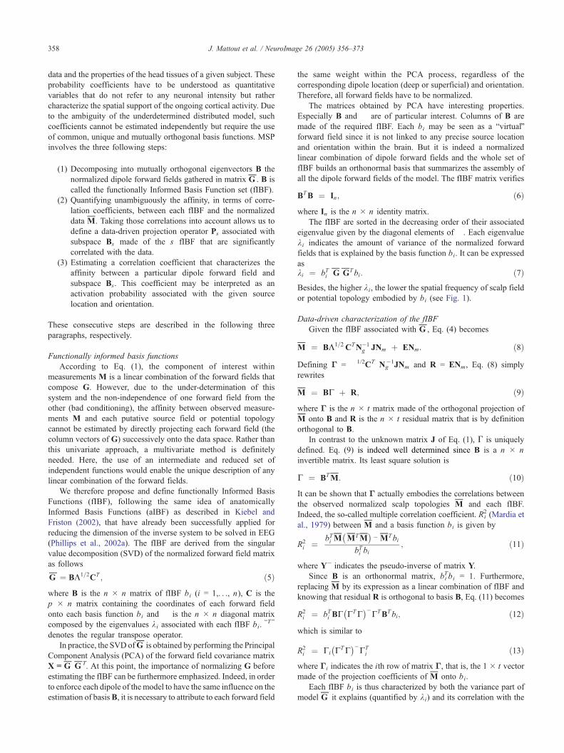
J. Mattout et al. / NeuroImage 26 (2005) 356–373358

data and the properties of the head tissues of a given subject. These

probability coefficients have to be understood as quantitative

variables that do not refer to any neuronal intensity but rather

characterize the spatial support of the ongoing cortical activity. Due

to the ambiguity of the underdetermined distributed model, such

coefficients cannot be estimated independently but require the use

of common, unique and mutually orthogonal basis functions. MSP

involves the three following steps:

(1) Decomposing into mutually orthogonal eigenvectors B the

normalized dipole forward fields gathered in matrix GP. B is

called the functionally Informed Basis Function set (fIBF).

(2) Quantifying unambiguously the affinity, in terms of corre-

lation coefficients, between each fIBF and the normalized

data MP. Taking those correlations into account allows us to

define a data-driven projection operator Ps associated with

subspace Bs made of the s fIBF that are significantly

correlated with the data.

(3) Estimating a correlation coefficient that characterizes the

affinity between a particular dipole forward field and

subspace Bs. This coefficient may be interpreted as an

activation probability associated with the given source

location and orientation.

These consecutive steps are described in the following three

paragraphs, respectively.

Functionally informed basis functions

According to Eq. (1), the component of interest within

measurements M is a linear combination of the forward fields that

compose G. However, due to the under-determination of this

system and the non-independence of one forward field from the

other (bad conditioning), the affinity between observed measure-

ments M and each putative source field or potential topology

cannot be estimated by directly projecting each forward field (the

column vectors of G) successively onto the data space. Rather than

this univariate approach, a multivariate method is definitely

needed. Here, the use of an intermediate and reduced set of

independent functions would enable the unique description of any

linear combination of the forward fields.

We therefore propose and define functionally Informed Basis

Functions (fIBF), following the same idea of anatomically

Informed Basis Functions (aIBF) as described in Kiebel and

Friston (2002), that have already been successfully applied for

reducing the dimension of the inverse system to be solved in EEG

(Phillips et al., 2002a). The fIBF are derived from the singular

value decomposition (SVD) of the normalized forward field matrix

as follows

GP ¼ BK1=2CT ; ð5Þ

where B is the n � n matrix of fIBF bi (i = 1,. . ., n), C is the

p � n matrix containing the coordinates of each forward field

onto each basis function bi and � is the n � n diagonal matrix

composed by the eigenvalues ki associated with each fIBF bi.bT Q

denotes the regular transpose operator.

In practice, the SVD ofGP

is obtained by performing the Principal

Component Analysis (PCA) of the forward field covariance matrix

X = GP

GPT. At this point, the importance of normalizing G before

estimating the fIBF can be furthermore emphasized. Indeed, in order

to enforce each dipole of the model to have the same influence on the

estimation of basisB, it is necessary to attribute to each forward field

the same weight within the PCA process, regardless of the

corresponding dipole location (deep or superficial) and orientation.

Therefore, all forward fields have to be normalized.

The matrices obtained by PCA have interesting properties.

Especially B and � are of particular interest. Columns of B are

made of the required fIBF. Each bi may be seen as a bvirtualQforward field since it is not linked to any precise source location

and orientation within the brain. But it is indeed a normalized

linear combination of dipole forward fields and the whole set of

fIBF builds an orthonormal basis that summarizes the assembly of

all the dipole forward fields of the model. The fIBF matrix verifies

BTB ¼ In; ð6Þ

where In is the n � n identity matrix.

The fIBF are sorted in the decreasing order of their associated

eigenvalue given by the diagonal elements of �. Each eigenvalue

ki indicates the amount of variance of the normalized forward

fields that is explained by the basis function bi. It can be expressed

aski ¼ bTi G

PGPTbi: ð7Þ

Besides, the higher ki, the lower the spatial frequency of scalp field

or potential topology embodied by bi (see Fig. 1).

Data-driven characterization of the fIBF

Given the fIBF associated with GP

, Eq. (4) becomes

MP ¼ BK1=2CTN�1

g JNm þ ENm: ð8Þ

Defining & = �1/2CT Ng�1JNm and R = ENm, Eq. (8) simply

rewrites

MP ¼ BC þ R; ð9Þ

where & is the n � t matrix made of the orthogonal projection of

MP

onto B and R is the n � t residual matrix that is by definition

orthogonal to B.

In contrast to the unknown matrix J of Eq. (1), G is uniquely

defined. Eq. (9) is indeed well determined since B is a n � n

invertible matrix. Its least square solution is

C ¼ BTMP: ð10Þ

It can be shown that & actually embodies the correlations between

the observed normalized scalp topologies MP

and each fIBF.

Indeed, the so-called multiple correlation coefficient. Ri2 (Mardia et

al., 1979) between MP

and a basis function bi is given by

R2i ¼

bTi MP

MPTM

P� �� MPTbi

bTi bi; ð11Þ

where Y� indicates the pseudo-inverse of matrix Y.

Since B is an orthonormal matrix, biTbi = 1. Furthermore,

replacing MP

by its expression as a linear combination of fIBF and

knowing that residual R is orthogonal to basis B, Eq. (11) becomes

R2i ¼ bTi BC CTC

� ��CTBTbi; ð12Þ

which is similar to

R2i ¼ Ci CTC

� ��CTi ð13Þ

where &i indicates the ith row of matrix &, that is, the 1 � t vector

made of the projection coefficients of MP

onto bi.

Each fIBF bi is thus characterized by both the variance part of

model GP

it explains (quantified by ki) and its correlation with the

Fig. 1. Illustration, using a MEG simulated data set (a), of the obtained functional Informed Basis Functions (b) and probability maps (c) given by the

Multivariate Source Prelocalization approach, and using a filtering based on the Velicer’s criterion.



normalized measurements MP

(quantified by Ri2). These two

quantities may be used to extract the few fIBF that present the

highest correlation with the data and that, taken together,

sufficiently explain the initial model GP

(see Appendix A.1). Such

a selection of a subset Bs of s basis functions amounts to filter both

the distributed source model and the data. It indeed removes the

component of GP

that does not significantly correlate with the

observed normalized topologies and also filters the noisy part of

the data that could only be explained by this removed model

component.

Deriving an activation coefficient for each dipole

On one hand, the selected subset Bs is characterized by its high

correlation with the normalized data. On the other hand, Bs

represents a component of model GP. Thus, defining M

Ps = BsBs

T MP

and projecting the normalized forward field of GP

onto MP

s, one

may identify the dipoles that are highly correlated with the

normalized measurement topologies.1 Indeed, the norm of this

projection quantifies the correlation between the considered

normalized forward field and the part of interest of the normalized

data. The projection operator is given by

Ps ¼ MP

s MTPs MP

s

� ��M

TPs: ð14Þ

As a projector, Ps does satisfy PsT = Ps and PsPs = Ps, hence the

norm of the projection of the normalized forward fields is given by

As ¼ GPT

Ps GP: ð15Þ

As is the p � p correlation matrix of the projected normalized

forward fields onto MP

s.

Two quantitative information can be derived from this matrix.

Firstly, the diagonal elements of As are probability-like co-

efficients of activation. Indeed, the closer to 1 such a coefficient, the

higher the correlation between the corresponding forward field and

the data part of interest. The cortical representation of those ac-

tivation coefficients leads to an activation probability map (APM,

see Fig. 1 for an example). This APM can then be used for restricting

the solution space to the few dipoles that are most likely to be

activated, by using a thresholding procedure which is performed

under the assumption of a Gamma distribution (see Appendix A.2).

Finally, the activation coefficients can also be introduced as quan-

titative functional priors within a regularized inverse procedure.

Secondly, the extra-diagonal elements of As quantify the

correlations between two different forward fields within the data

subspace defined byPMs. The closer to 0 this correlation, the more

complementary the two considered dipoles for explaining the data

part of interest. Conversely, the closer to 1 the absolute value of

this correlation, the more redundant the information explained by

each of the two dipoles. This data-driven estimation of the

correlation between two different forward fields leads to comple-

mentarity probability maps (CPM) that give a sight of the

activation source configuration which is totally different from the

one given by the APM or any other conventional activation map.

Indeed, let us define

aij ¼ A2s i; jð Þ

As i; ið ÞdAs j; jð Þ ; ð16Þ

where As (i, j) indicates the ith row and j th column element of As.

aij is nothing but the square of the cosine of the angle between the

1 Note that the product BsBsT defines an orthogonal projection matrix.

projected normalized forward fields associated with dipoles i and j,

respectively. Given a dipole i, computing coefficient aij for each

dipole j of the distributed model leads to the CPM related to dipole

i. The closer to zero aij, the more complementary dipoles i and j

for explaining the data. Assuming that dipole i is activated, the

related CPM indicates whether the other dipoles should be

activated or not in order to improve the explanation of the

measured scalp distributions (see Fig. 1 for an example).

In this paper, we focus on the information given by the diagonal

elements of As, the APM. Note finally that the calculation of the

single matrix As is based upon a t sample-wide data window.

Consequently, the more stationary the activity within that time

window, the more reliable the estimated correlation matrix.

Application

We performed numerical simulations in order to validate and

evaluate the performance of the MSP approach as a prelocalization

method as well as a better conditioning tool preceding any source

estimation. We studied the performances of MSP under the

variation of different parameters such as the number of simulated

sources, the width of the data window and the noise level. We also

compared, within the MSP process, different ways of selecting the

fIBF as well as the effect, on the regularization inverse procedure,

of the thresholding of the obtained APM. Those numerical

simulations enabled us to derive an optimal MSP procedure which

was finally evaluated on real MEG data. The simulation studies,

the real data experiment and the way we analyzed the results are

detailed in this section. The results themselves are presented in the

next section.

Simulation studies

MEG data simulation

Since the MEG/EEG sources are widely believed to be

restricted to the pyramidal neuron cells of the cortical strip (Nunez

and Silberstein, 2000), a common approach within the distributed

model framework consists of constraining the dipoles to be

distributed onto the cortical surface extracted from a structural

Magnetic Resonance Imaging (MRI) volume (Dale and Sereno,

1993). After following the segmentation of the MRI volume,

dipoles are typically located at each node of a triangular mesh of

the white/grey matter interface (Mangin, 1995). Furthermore, since

the apical dendrites of these cortical neurons are organized

perpendicularly to the surface, the corresponding dipoles are also

constrained to have this particular orientation.

In order to simulate MEG data, a 3D high resolution (voxel

size: 0.9375 mm � 0.9375 mm � 1.5 mm) MRI volume from a

healthy volunteer was segmented. The boundary between white

and grey matter was approximated with small triangles whose

vertices provided 7081 dipole positions uniformly spread all over

the cortex. The spatial resolution was high enough to well describe

the cortical topology, since the mean distance between two

neighboring dipoles was about 3 mm.

We calculated the forward operator G corresponding to this

dipole mesh. Since head tissues are non-magnetic, estimating the

matrix G by solving the electromagnetic equations does not

require a precise description of the geometrical and electro-

magnetic properties of the head. We therefore simply designed a

one-layer sphere head model, which allowed us to calculate an


analytical solution of the equations of magnetic field propagation

(Sarvas, 1987).

MEG data were simulated over 130 sensors uniformly spread all

over the head, by artificially activating either one or two extended

sources. Each extended source was defined by a randomly chosen

cluster of neighboring dipoles of the cortical mesh. The spatial

extent of the source was also randomly determined and varied from

0 mm2 (case of a pin-point source or single dipole) to about 80 mm2

(a cluster comprising five dipoles).

We considered unit amplitude for each source and its

contribution to the measurements was given by averaging the

forward fields of the dipoles belonging to the active cluster. The

time course of the activation was modeled as the half-period of a

sine function. The contribution of each source was convolved by

its associated time course and the resulting waveforms were added

together to constitute the data. When simulating two active

sources, a delay of two time samples was set between the two

related waveforms. A white Gaussian noise was finally added to

each simulated data set and the full signal was sampled over 15

time points (see Fig. 1 for an example).

The different varying parameters of our simulations are listed

below. Whatever the number of simulated areas (one or two), we

have been considering:

! Either a small (SW) or a large (LW) data window to be

processed by MSP. SW contained the signal peak and its two

closest neighboring time samples, while LW corresponded to

the eleven-sample-wide data window centered on the signal

peak.

! Three different noise levels: no noise (NN), a fairly realistic

noise (RN, SNR = 20 dB) when considering averaged data

and a relatively high noise (HN, SNR = 14 dB). The signal-to-

noise ratio (SNR) was thus fixed by setting the noise

amplitude to the appropriate value with respect to the

maximum amplitude of the simulated signal over the whole

data window.

! Two ways of selecting the fIBF that are significantly correlated

with the measurements: a filter based on an explained variance

criterion (EVF, see Appendix A.1.1) and a filter based on

Velicer’s criterion (VCF, see Appendix A.1.2).

In the two following paragraphs, we describe the simulation

experiments performed in order to, on the one hand, study the

performance of MSP per se and, on the other hand, evaluate MSP

ability to better condition a linear inverse estimation. Thanks to

the factorial nature of these two simulation studies, we performed

statistical analysis on the obtained values of the evaluation

criteria described hereafter. This enabled us to synthesize and

highlight the main concepts and performance of the proposed

approach. When appropriate, we thus performed Analyses of

Variance (ANOVA) accounting for non-sphericity and used

Scheffe’s statistic as post hoc test (this was performed using

the SPSS 11.0 software).

Quantitative evaluation of MSP performance

The single source configuration is the simplest one and should

not require any multivariate approach since the data directly

correspond to the sum of a single gain vector (scaled by an

amplitude factor) and some measurement noise. Nevertheless, it is

worth while to study in order to both evaluate MSP performance

and infer its robustness to some parameters such as the noise level

and the width of the data window processed and to be compared

with a multiple activated source configuration.

We considered here two data window widths (SW and LW), the

three noise levels (NN, RN and HN) but no fIBF-based filtering

(NOF).

On the other hand, with two activated sources, we not only let

the window size and the noise level vary, but also considered the

two proposed fIBF-based filtering methods (EVF and VCF). Such

filtering approaches were only applied when noise was corrupting

the data (RN and HN configurations).

For both the single source and the two sources configurations,

1000 randomly chosen source locations were successively consid-

ered. The two following criteria were then used to quantify MSP

performance:

! The rank of the simulated dipoles when considering their

estimated activation probability. This information was used to

present performance curves and tables. Given some particular

conditions (the size of the data window, the noise level and the

filtering approach), a performance curve was defined as the

percentage of source configurations for which the activated

sources were recovered within the subset of dipoles that

presented the highest activation probability values, plotted

against the size of this subset. A simulated source was

considered as being recovered as soon as at least one of its

dipole belonged to the subset.

! The Pre-Localization Error (PLE), defined as the distance

between a simulated activated cortical region and its closest

APM local maximum. This quantitative criterion can be

suitably displayed using histograms showing the percentage

of simulation configurations for which the PLE ranged within

a certain distance band. In practice, when considering one

single activated source, the PLE was defined as the distance

between the true source and the location of the global APM

maximum. When considering two activated sources, the cortex

was first split into two parts which corresponded to the dipoles

that were closer to the first (resp. the second) true activated

source. The PLE for each simulated dipole was defined as the

distance between the true dipole itself and the location of the

maximum of the APM previously restricted to the correspond-

ing cortical partition. Then, the final PLE associated with the

two activated sources was defined as the mean of the two

PLEs.

These two criteria are complementary. The first one informs us

about the ability of MSP to allocate a high probability of activation

to the true activated dipoles, whereas the PLE informs us about the

spatial error induced when attributing such a high activation

probability.

Quantitative evaluation of the better conditioning induced by MSP

The results of the first experiment allowed us to identify and set

some optimal parameter values before performing this second

simulation study. Indeed, while still dealing with either one or two

activated sources, we only considered the large data window (LW)

and the filtering based on Velicer’s criterion (VCF). We also

restricted this simulation experiment to the realistic noise level case

(RN = 20 dB) since it corresponds to the usual framework for

applying inverse solutions (averaged epoch data).

One hundred randomly chosen locations of both configurations

(single source and pair of sources) were tested.

2 Note that the ECD solutions were used here in place of a better

reference and did not aim at being compared in terms of localization

performance to the evaluated distributed solutions. They rather enabled us

to assess the face validity of the WMN constrained by MSP.


As a classical inverse approach, we used the linear solution

given by the unique minimum of the quadratic criterion

U Jð Þ ¼ NM � GJN2 þ ENWJN2; ð17Þ

also known as the weighted minimum norm solution (WMN),

where W is a p � p diagonal weighting matrix and E is a

regularization parameter (or hyperparameter), which was estimated

by the empirical bL-curve Q approach (Gorodnitsky et al., 1995).

jjAjj2 denotes the L2-norm of matrix A.

The WMN solution is given by

JWMN ¼ GTG þ EWTW� ��1

GTM; ð18Þwhich, according to the Matrix Inversion Lemma, is equivalent to

JWMN ¼ WTW� ��1

GT G WTW� ��1

GT þ EIn� ��1

M: ð19Þ

Each inverse solution was performed for the single time sample

corresponding to the signal peak. For each simulated data set,

depending on the choice of W and the size of the solution space,

the four following inverse solutions were implemented:

(1) TI (total-identity): WMN solution calculated on the initial

global set of dipoles and without introducing any quantita-

tive prior (W = Ip);

(2) RI (restricted-identity); WMN solution calculated on the

restricted number of dipoles that corresponded to the dipoles

remaining after thresholding the APM (see Appendix A.2)

and without introducing any quantitative prior (W = Ip);

(3) TM (total-MSP); WMN solution calculated on the initial

global set of dipoles and involving quantitative priors de-

rived from the APM (for each dipole i, W(i, i) = 1 � As (i)).

The closer to 1 the activation probability As(i), the more the

absolute amplitude of dipole i is enforced to be high;

(4) RM (restricted-MSP); WMN solution applied on the

restricted number of dipoles that corresponded to the dipoles

remaining after thresholding the APM and involving the

quantitative priors derived from the APM.

Moreover, all these inverse solutions were applied to both:

(1) The raw data M (RD),

(2) The filtered data Mf (FD) obtained using the filter based on

Velicer’s criterion (see Appendix A.1.2).

We thus ended up with eight different reconstructions which were

compared using the two following evaluation criteria:

! The Localization Error (LE), defined as the distance between

the true activated source and the dipole of maximum estimated

amplitude. In case of two simulated clusters, the same

procedure of cortical partitioning as for the study on MSP

performance was implemented, in order to estimate the LE

associated with each activated source.

! The Root Mean Square Error (RMSE) given by

RMSE ¼

ffiffiffiffiffiffiffiffiffiffiffiffiffiffiffiffiffiffiffiffiffiffiffiffiffiffiffiffiffiffiffiffiffiffiffiffiffiffiffiffiffiffiffiffiffiffiffiffiffiffiffiffiffiffiffiffiffiffiffiffiffiffiffiffiffiffiffiJJ

maxi jJJ ið Þj� Jref

maxijJref ið Þj

�2

;

vuut ð20Þ

where J and Jref indicate the estimated and the simulated

distributions of amplitude, respectively.

The closer to zero the value of LE, the more precise the

localization of the source. However, when comparing two inverse

solutions (J1 and J2), one should notice that even though RMSE1

V RMSE2, one still requires LE1 V LE2 to conclude that J1 gives a

better estimation than J2 (Phillips et al., 2002a).

Real MEG data experiment

Somatosensory-evoked fields

The effectiveness of the proposed algorithm was also evaluated

using data from a real somatosensory MEG experiment. The data

acquisition was conducted using a whole-scalp magnetometer

(CTF Systems Inc. Omega 151 channels). The somatosensory

stimulation was an electrical square-wave pulse (0.2 ms duration,

set at twice the perceptual threshold) delivered randomly to the

thumb, index, middle and little finger of each hand of a healthy

right-handed subject (Meunier et al., 2001). Interstimulus interval

ranged from 350 ms to 550 ms and four hundred evoked magnetic

field responses were averaged for each finger. Data were sampled

at 2500 Hz and filtered between 0 and 800 Hz. For the purpose of

the current evaluation, only data from the right index and right

little finger were considered. The data window of interest was

located around the major peak recorded within the first 50 ms

after stimulation (cf. Figs. 2 and 3). This peak mostly corre-

sponded to the activation of the primary somatosensory cortex

(S1).

A distributed model of the cortical sheet, composed of 7205

dipoles, was built using the subject’s structural MRI and following

the same procedure as described in the simulation studies section.

Based on the results of the two simulation experiments, MSP was

applied on the largest coherent data window, that is the whole peak

of interest. AVelicer-based filtering was considered. The APM was

then thresholded assuming a Gamma distribution of the estimated

activation probabilities all over the cortex. Finally, the WMN

inverse solution spatially restricted and quantitatively constrained

by the thresholded APM (RM solution) was performed on the

filtered data, for the time sample corresponding to the signal peak

(cf. Figs. 2 and 3).

Evaluation criteria

In the absence of a gold standard when dealing with real

data, we used an equivalent current dipole (ECD) solution

performed on the same data sample and involving the same

forward operator based on a single sphere head model. Only

ECDs accounting for at least 80% of the measured field variance

were accepted. It led to the estimation of one ECD for each

finger. The ECD solution was quite reliable in that case, since

only a single and focal activated cortical area was expected (in

the postcentral gyrus).2

Quantitatively, we used the two following measures:

! The PLE of the maximum of the APM with respect to the

location of the estimated ECD;

! The LE of the reconstructed dipole of maximum absolute

amplitude with respect to the same ECD reference.

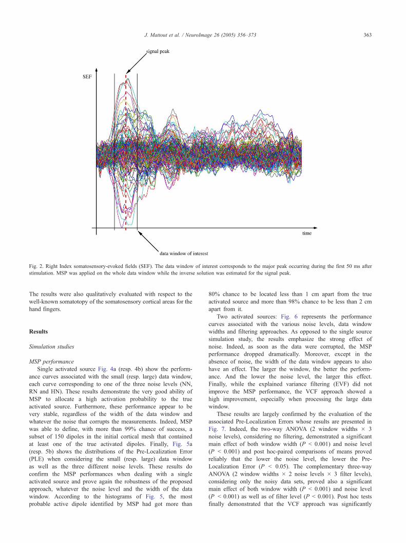
Fig. 2. Right Index somatosensory-evoked fields (SEF). The data window of interest corresponds to the major peak occurring during the first 50 ms after

stimulation. MSP was applied on the whole data window while the inverse solution was estimated for the signal peak.


The results were also qualitatively evaluated with respect to the

well-known somatotopy of the somatosensory cortical areas for the

hand fingers.

Results

Simulation studies

MSP performance

Single activated source Fig. 4a (resp. 4b) show the perform-

ance curves associated with the small (resp. large) data window,

each curve corresponding to one of the three noise levels (NN,

RN and HN). These results demonstrate the very good ability of

MSP to allocate a high activation probability to the true

activated source. Furthermore, these performance appear to be

very stable, regardless of the width of the data window and

whatever the noise that corrupts the measurements. Indeed, MSP

was able to define, with more than 99% chance of success, a

subset of 150 dipoles in the initial cortical mesh that contained

at least one of the true activated dipoles. Finally, Fig. 5a

(resp. 5b) shows the distributions of the Pre-Localization Error

(PLE) when considering the small (resp. large) data window

as well as the three different noise levels. These results do

confirm the MSP performances when dealing with a single

activated source and prove again the robustness of the proposed

approach, whatever the noise level and the width of the data

window. According to the histograms of Fig. 5, the most

probable active dipole identified by MSP had got more than

80% chance to be located less than 1 cm apart from the true

activated source and more than 98% chance to be less than 2 cm

apart from it.

Two activated sources: Fig. 6 represents the performance

curves associated with the various noise levels, data window

widths and filtering approaches. As opposed to the single source

simulation study, the results emphasize the strong effect of

noise. Indeed, as soon as the data were corrupted, the MSP

performance dropped dramatically. Moreover, except in the

absence of noise, the width of the data window appears to also

have an effect. The larger the window, the better the perform-

ance. And the lower the noise level, the larger this effect.

Finally, while the explained variance filtering (EVF) did not

improve the MSP performance, the VCF approach showed a

high improvement, especially when processing the large data

window.

These results are largely confirmed by the evaluation of the

associated Pre-Localization Errors whose results are presented in

Fig. 7. Indeed, the two-way ANOVA (2 window widths � 3

noise levels), considering no filtering, demonstrated a significant

main effect of both window width (P b 0.001) and noise level

(P b 0.001) and post hoc-paired comparisons of means proved

reliably that the lower the noise level, the lower the Pre-

Localization Error (P b 0.05). The complementary three-way

ANOVA (2 window widths � 2 noise levels � 3 filter levels),

considering only the noisy data sets, proved also a significant

main effect of both window width (P b 0.001) and noise level

(P b 0.001) as well as of filter level (P b 0.001). Post hoc tests

finally demonstrated that the VCF approach was significantly

Fig. 3. Little finger somatosensory-evoked fields (SEF). The data window of interest corresponds to the major peak occurring during the first 50 ms after

stimulation. MSP was applied on the whole data window while the inverse solution was estimated for the signal peak.


better than both NOF and EVF (P b 0.001) but also that NOF

was significantly better than EVF (P b 0.001).

To conclude, the most favorable manner for applying MSP

appears to be by considering the large data window and the

filtering based on Velicer’s criterion.

Better conditioning induced by MSP

Following the results of the above simulation study, MSP

was applied on the large data window and involved the filtering

based on Velicer’s criterion. Thanks to this filtering approach,

the inverse operator could also be applied on the filtered data

(FD).

Single activated source: Fig. 8 and Table 1 show the

quantitative results in terms of Localization Error (LE) and Root

Mean Square Error (RMSE), respectively.

Concerning the LE criterion, it first appears that the local-

izations were much better when the inverse solution was

quantitatively constrained using the APM (TM and RM solutions)

than when it was unconstrained. Moreover, the results were also

improved when estimating the inverse solution on the filtered

data rather than directly on the raw data. Indeed, the two-way

ANOVA (2 data preprocessing � 4 inverse solutions) demon-

strated a reliable main effect of both factors (P b 0.001). Then,

Scheffe’s tests showed a significant improvement when using TM

and RM solutions compared to either TI or RI (P b 0.001). They

also showed significantly lower LE with TI than with RI (P b

0.001). However, the performance of TM and RM did not appear

to be significantly different.

Similar conclusions can be drawn from the RMSE criterion in

terms of quality of the estimated distribution of activity (cf. Table

3). Indeed, the two-way ANOVA (2 data preprocessing � 4

inverse solutions) demonstrated a reliable main effect of both

factors (P b 0.001). Moreover, Scheffe’s tests showed a significant

improvement when using TM and RM solutions compared to

either TI or RI (P b 0.001). It also failed showing any reliable

difference between TM and RM estimated distributions. Finally,

RI proved significantly better than TI according to the RMSE

criterion (P b 0.001). Note however that this last result was quite

meaningless since TI showed a reliable lower LE than RI.

It is important to notice that restricting the number of dipoles

did not bring any advantage. It may even lead to worse results in

terms of LE, like when comparing TI and RI approaches.

Summarizing this first evaluation based on both LE and RMSE

criteria, the best inverse approaches are those involving the APM

given by MSP (TM and RM approaches) and even better results are

obtained when performing the data filtering enabled by the MSP

process.

Two activated sources: in that more difficult case, Fig. 9 and

Table 2 show the quantitative results in terms of Localization Error

(LE) and Root Mean Square Error (RMSE), respectively. These

results were consistent with those obtained for a single activated

source. The TM and RM inverse solutions were closer to the true

Fig. 4. Single source configuration. Performance curves considering the small (a) and the large (b) data window as well as the different noise levels.


solutions than the TI and RI ones. Moreover, filtering the data did

further improve the results.

Indeed, the two-way ANOVA (2 data preprocessing � 4

inverse solutions) demonstrated a reliable main effect of both

factors (P b 0.001). Then Scheffe’s tests showed a signifi-

cant decrease of the LE when performing TM and RM com-

pare to either TI or RI (P b 0.001) but did not show

any reliable difference between TM and RM, nor between TI

and RI.

The RMSE criterion testified the better results obtained with

TM and RM than with TI and RI inverse approaches. But the

quality of the distribution was not significantly improved neither

by the data filtering, nor by restricting the solution space and

computing RM instead of TM inverse solution. Indeed, the two-

way ANOVA (2 data preprocessing � 4 inverse solutions) here

demonstrated a reliable main effect of the inverse solution (P b

0.001) but did not show any significant main effect of the data

preprocessing. Furthermore, Scheffe’s tests showed significant

better RMSE for TM and RM than for both RI and TI (P b 0.001)

as well as reliable lower RMSE for RI than for TI (P b 0.001). On

the other hand, no reliable difference could be assessed between

RM and TM.

Real MEG data experiment

Figs. 10 and 11 represent the APM, the thresholded APM, the

estimated amplitude map and the reconstructed ECD for

the index and the little finger data, respectively. For both

fingers, the APM and thresholded APM exhibited two main

regions of activity. As expected, the most probable one was

located around the contro-lateral postcentral gyrus whereas the

second area was in the ipsi-lateral temporal lobe. Thresholding

the index (resp. little finger) APM led to a subset of 553 (resp.

636) dipoles. In both cases, the reconstructed amplitude maps

based on each thresholded APM showed a single and focal

activation spot which appeared to be consistent with the

corresponding ECD location. Moreover, the relative location of

these two spots was in keeping with the well-known somatotopy

of the hand fingers along the postcentral gyrus (Meunier et al.,

2001).

Fig. 5. Single source configuration. PLE histograms considering the small

(a) and the large (b) data window as well as the different noise levels.


Finally, Table 3 gives the PLE and LE values associated with

these maps given the respective ECD references. For both the

index and the little finger, the most probable region of activation as

well as the reconstructed spot of activity were found less than 1 cm

away from the estimated ECD.

Discussion

Methods

In the present paper, the new Multivariate Source Prelocaliza-

tion (MSP) approach has been described in details, validated and

evaluated on both simulated and real MEG data. This method is

directly applicable to EEG data but remains to be evaluated in that

context. Quantitative differences in the results might be observed

since the EEG and MEG signatures of a given brain area are

inherently different.

MSP consists of three consecutive steps. The first one consists

of building a set of functionally informed basis functions (fIBF).

These fIBF are uniquely defined as being the eigenvectors given

by the principal component analysis (PCA) of the normalized

forward operator covariance matrix. Contrary to the customary use

of PCA or independent component analysis (ICA) (Kobayashi et

al., 2002; Mosher and Leahy, 1998), the multidimensional analysis

process is here conducted on the forward model rather than on the

MEG/EEG data itself. The fIBF are thus specific to the anatomo-

functional properties of each subject and do not depend on the data

to be analyzed. They remain the same for a whole recording

session (for a given experimental setup). FIBF aim at summarizing

all the putative scalp measurements due to the simultaneous

activation of cortical sources. PCA is particularly suitable for

achieving such a goal. Indeed, PCA-derived fIBF are as few as the

number of sensors. They are mutually orthogonal and linearly

related to each source forward field of the model. Finally, due to

the principle of PCA itself, the higher the variance of the forward

model accounted for a given fIBF, the lower the spatial frequency

of the scalp representation of this fIBF. This property supports the

usefulness of PCA-derived fIBF for then separating the data part of

interest from noise. The signal that stems from cortical source

activation indeed corresponds to low spatial frequency maps

whereas scalp representations of noise rather lie in high spatial

frequency bands.

Although MSP is not an inverse method, note that, similarly to

part of the process of beamforming approaches, MSP estimates

from the data a quantitative prior which defines a regularization

weight for each brain region separately (Hauk, 2004). However,

beamformers such as Synthetic Aperture Magnetometry (SAM)

have difficulty analyzing highly temporally correlated sources such

as the ones simulated here (Vrba and Robinson, 2001), whereas

MSP exploits the normalized stationary scalp topologies and does

not assume any temporal decorrelation between sources. Beam-

forming techniques are therefore more suitable for analyzing large

data windows while MSP is limited by the consistency of the

underlying spatial activity. Actually, MSP (when no filtering and

no dimension reduction are performed) could be more closely

related to the data-driven regularization early proposed in (Dale

and Sereno, 1993). However, a crucial difference lies in that MSP

involves a normalization step, which leads to the concept of fIBF

and initiates the important dissociation between the localization

and estimation issues.

Through the essential intermediate of fIBF, MSP produces a

uniquely-defined probability-like coefficient of activation for each

source of the model. The fIBF both enforce the uniqueness of the

probability estimation and make the process multivariate, which

means that correlations between all the different explicative

sources are taken into account. The fIBF are positively the key

functions that enable one to achieve MSP’s objective. But besides,

one could foresee some further applications of such fIBF. At the

single subject level, one could investigate their usefulness for

quantitatively establishing the complementarity of EEG and MEG

measurements and optimizing a common inverse procedure as

proposed in Baillet et al. (1999), Babiloni et al. (2001) and Fuchs

et al. (1998). At the group level, fIBF might be profitably

compared between subjects in order to infer the common and

different aspects of cortical activities by subjects who performed

the same experimental task.

We proposed two ways of selecting the subset of fIBF that best

characterizes the data part of interest. This second step involves

only the data and amounts to filter both the measurements and the

forward model components. The advantage of such a filtering is

twofold: improving the MSP process itself as well as facilitating

Fig. 6. Two sources. Performance curves considering the three noise levels, the two data window sizes and successively preforming no filtering at all (a, b), the

filtering based on explained variance (c, d) and the filtering based on Velicer’s criterion (e, f ).


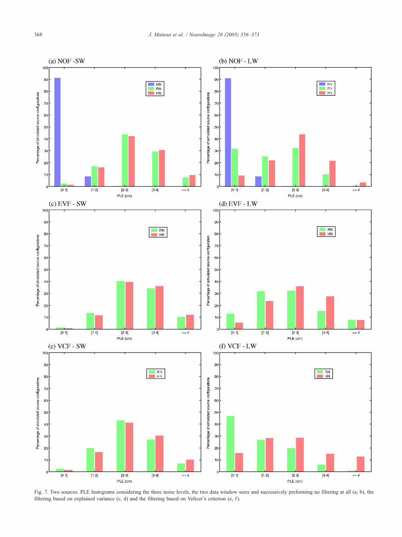
Fig. 7. Two sources. PLE histograms considering the three noise levels, the two data window sizes and successively preforming no filtering at all (a, b), the

filtering based on explained variance (c, d) and the filtering based on Velicer’s criterion (e, f ).


Fig. 8. Single source. LE histograms comparing of the four inverse

solutions (TI, RI, TM and RM) when processing either the raw data (a) or

the filtered data (b).

Fig. 9. Two sources. LE histograms comparing the four inverse solutions

(TI, RI, TM and RM) when processing either the raw data (a) or the filtered

data (b).


the subsequent inverse approach that would exploit the so-filtered

data. However, such a filtering is not strictly needed as soon as the

third and last projection step takes the correlation of each fIBF with

the data into account. This multivariate projection leads to the

estimation of cortical activation probability maps (APM) and

complementarity probability maps (CPM).

APM can be thresholded under the assumption of a Gamma

distribution, thus reducing the solution space to the few sources

Table 1

Single source

TI RI TM RM

RD 9.8 (2.3) 4.7 (0.9) 1.9 (0.9) 1.9 (0.7)

FD 11.1 (3.2) 6.1 (1.6) 1.7 (0.9) 1.6 (0.8)

Mean RMSE values (and associated standard error in parentheses)

comparing the four inverse solutions (TI, RI, TM and RM) when processing

either the raw data or the filtered data.

that are most likely to be activated. The APM values can also be

used as quantitative priors within any regularization approach for

solving the MEG/EEG inverse problem. The evaluation of the

quality and the usefulness of the APM were the core of this paper.

However, the CPM are also of a particular interest. For a given

dipole of the model, the associated CPM indicates whether each

other dipole is complementary or redundant for explaining the data.

This type of information is usually neglected when attempting to

Table 2

Two sources

TI RI TM RM

RD 10.9 (2.0) 5.3 (0.9) 2.8 (0.8) 2.6 (0.6)

FD 11.0 (3.0) 6.0 (1.4) 2.5 (0.6) 2.4 (0.6)

Mean RMSE values (and associated standard error in parentheses)

comparing the four inverse solutions (TI, RI, TM and RM) when processing

either the raw data or the filtered data.

Fig. 10. Index—front view: APM (a), thresholded APM (b), RM inverse

solution whose values have been normalized to range from 0 to 1 (c) and

cortical area corresponding to the ECD (d).

Fig. 11. Little finger—front view: APM (a), thresholded APM (b), RM

inverse solution whose values have been normalized to range from 0 to 1

(c) and cortical area corresponding to the ECD solution (d).

Table 3

Real MEG data

PLE (cm) LE (cm)

Index 0.5 0.4

Little finger 0.7 0.7

For both fingers, distance between the ECD solution and the APM

maximum (PLE) and distance between the ECD solution and the dipole of

maximum absolute reconstructed amplitude (LE).


solve the MEG/EEG inverse problem but deserves to be further

investigated. It might be exploited in a way similar to the non-data-

driven crosstalk and point spread metrics that have been recently

used for inferring the source localization accuracy when involving

a distributed source model and a linear inverse operator (Grave de

Peralta Menendez et al., 1996; Liu et al., 2002).

It is finally important to emphasize the originality of the MSP

approach which, by normalizing the data and the forward operator,

focuses on the source localization but not on the estimation issue.

In the next future, the diagonal normalization matrices Nm and Ng

might be considered as metric operators and be adapted to

incorporate priors, such as between-sensors or between-sources

correlations, from the early stage of fIBF construction.

Results

In order to demonstrate the effectiveness of the new proposed

method, we performed simulations for evaluating MSP as both a

prelocalization process and a preprocessing tool for better

conditioning the source reconstruction.

We studied the effect of several parameters such as the noise

level, the width of the data window to be processed and the

number of activated sources. Considering a large number of

randomly chosen source configurations, the first simulation

experiment demonstrated clearly the high ability of MSP to

prelocalize the activated sources. As expected, the two-activated

source case is more difficult to deal with than the one-activated

source one. This quite large degradation of the performance might

be due to the substantial difference between a non-ambiguous

source distribution (a single source elicits a single scalp topology)

and an ambiguous one (several active sources with non-

independent scalp contributions do produce ambiguous data).

Although it remains to be tested, we might thus observe that the

further degradation then caused by moving from a two source

configuration to a three or four source configuration would be

much less important than the one we here observe when departing

from the unambiguous single source case. Moreover, this

degradation might highly depend upon the relative source location

and orientation which is somehow quantified by the CPM

coefficients and could be profitably exploited to further constrain

the source estimation.

Nevertheless, results can be significantly improved by imple-

menting the filtering approach based on Velicer’s criterion and

considering the largest coherent data window, even when the data

are corrupted by noise. The largest coherent data window refers to

all the recorded time samples that reflect the same cortical activity.

Indeed, the more data samples associated with the same cortical

activity, the better the fIBF selection and data filtering and the

higher the chance of prelocalizing the true activated sources.


However, other filtering approaches might be tested, such as a

stepwise iterative process for selecting the fIBF that are signifi-

cantly sufficient for explaining most of the measurements.

One has to keep in mind that MSP does not fully solve the

inverse problem and the usefulness of the APM for improving the

source reconstruction had therefore to be assessed. Within the

scope of a regularized linear inverse operator, the second

simulation experiment enabled us to demonstrate and assess the

better conditioning due to MSP. In the condition of realistic noise

and two activated cortical sites, the use of APM-derived

information significantly improved the source reconstruction

compared to the classical unweighted minimum norm solution.

Moreover, this important improvement when reconstructing the

sources was observed in terms of both source localization and

amplitude estimation. As expected, filtering the data improved the

results even further. However, these good results were mainly due

to the introduction of the activation probabilities as local

regularization weights, rather than to the reduction of the solution

space resulting from the thresholding of the APM. Indeed, the RM

solution did not prove significantly better than the TM one. It could

be explained by a too conservative thresholding of the APM. On

the one hand, restricting the solution space led to a less

underdetermined system to be solved and to a more focal inverse

solution that was easier to be interpreted. On the other hand, such a

restriction might mislead the reconstruction process since some

true activated source might have been removed from the solution

space. In view of the only slight advantage of restricting the

solution space, one may rather choose the TM approach, especially

if more than two cortical sites are expected to be activated.

Finally, one has to keep in mind that if simulations are needed

and reliable for validating and evaluating any new methodology,

they cannot be fully satisfactory. We here only dealt with up to two

activated sites, white noise and activated sources that were well

separated spatially. Moreover, simulations remove the effect of

forward problem errors. This explains why we also validated and

evaluated the MSP process on a sample of real MEG data.

Nevertheless, more suitable configurations might also be met with

real data than with simulated data. For instance, coherent data

windows comprising more than 11 samples might easily be

observed. Furthermore, in some applications such as the local-

ization of epileptic foci from averaged spikes, the signal-to-noise

ratio can be higher than 20 dB.

Conclusion and perspectives

In this paper, we presented the MSP approach and showed its

value for prelocalizing the cortical sources of MEG measures and

for better conditioning the full reconstruction in terms of location

and amplitude estimation. Moreover, MSP gives several qualitative

and quantitative useful informations such as APM. APM can be

first simply displayed for having an idea of the distribution of the

cortical activity. APM can also be thresholded in order to

emphasize the cortical sites that are most likely to explain the

data. These locations could be even exploited for the initialization

of the ECD inverse methods. Note however that ECD methods

would have difficulty incorporating the quantitative information

from the APM compared to distributed model-based approaches.

Quantitatively, the APM proved efficient for better conditioning a

constrained linear inverse operator. Such constraints could be

easily adapted and tested on other inverse approaches such as

FOCUSS (Gorodnitsky et al., 1995; Mattout et al., 2004) and

LORETA (Pascual-Marqui et al., 1994). Besides, it is important to

notice that MSP-derived constraints arise from the MEG/EEG data

itself. By contrast to other regularization approaches that rely upon

external functional priors such as those given by fMRI (Dale et al.,

2000), MSP enables one to constraint the inverse problem by

simply preprocessing the MEG/EEG measures. Such constraints

are more reliable than any others and could be profitably coupled

with other external priors in order to balance the possible

misleading effect of between-modality fusion. Finally, through

the use of fIBF, MSP is also a data-filtering tool.

In the next future, the accuracy and usefulness of both APM

and CPM have to be further investigated on both EEG and MEG

data, simulated and real experiments (Daunizeau et al., 2004). The

fIBF might be coupled with anatomical Informed Basis Functions

in order to further develop an optimal and data-driven description

of the solution space that would at best support the source

reconstruction. These developments might also take advantage of

recently proposed approaches for the automatic estimation of

regularization parameters (Phillips et al., 2002b). Finally, dedicated

inverse approaches can be developed for especially optimizing the

coupling between MSP and a weighted linear inverse operator

(Mattout et al., 2003).

Acknowledgments

Authors are grateful to Dr. Sabine Meunier (Department of

Clinical Neurophysiology, Pitie-Salpetriere Hospital, Paris, France)

for providing us with the real MEG data. Jeremie Mattout is funded

by an EC Marie Curie fellowship.

Appendix A

A.1. fIBF Filtering

The functionally Informed Basis Functions (fIBF) are given by

the first step of the MSP process. It consists in the principal

component analysis (PCA) of the forward operator associated with

a particular subject and experimental session. fIBF can be

classified according to their affinity with the measurements in

order to infer the corresponding activation probability map (APM)

at best. This classification enables to select fIBF according to some

criterion. We here proposed and tested two such selections or

filtering approaches which are based on two different criteria.

A.1.1. Filtering based on explained variance (EVF)

As explained in the theory section, each fIBF bi is characterized

by:

! An eigenvalue ki which quantifies the variance part of model GP

that is explained by bi,

! A coefficient Ri2 which quantifies the variance part of measure-

ments MP

that is explained by bi.

The filtering is based on these two quantities and aims at

identifying the few fIBF that significantly and sufficiently explain

both the model and the data. The fIBF are thus sorted in the

decreasing order of their multiple correlation coefficient Ri2. A

subset Bs made of the highest-ranked fIBF is then defined such as


it explains a sufficient amount of variance of the model. In practice,

we defined Bs as the smallest subset that explains at least 85% of

the variance of the model. The percentage I s of explained variance

is given by

I s ¼ 100�

PE j

j a BsPE j

j a B

: ð21Þ

A.1.2. Filtering based on Velicer’s criterion (VCF)

The second approach proceeds the other way round. It seeks for

the subset Bn�s made of the n � s fIBF that, taken together, both

correspond to the noisy part of the measurements and explain the

smallest part of the model variance. This can be achieved by

minimizing Velicer’s criterion (Velicer, 1976). To do so, the fIBF

are sorted in the decreasing order of their eigenvalues Ei and the

criterion r(s) is calculated for each pair (Bs,Bn � s) of comple-

mentary subsets. It is given by

v sð Þ ¼ 1

n n� 1ð ÞXn

j;k ¼ 1

j p k

r 2s j; kð Þ; ð22Þ

where rs2 ( j, k) is the partial correlation between data samples j and

k, having removed the part of the data explained by the first s fIBF.

This removal is simply performed by the orthogonal projection

of the data samples onto Bn � s. Thus the number q of fIBF that

minimizes Velicer’s criterion indicates the subset Bn � q onto which

the sum of the partial correlations between data samples is

minimum. In other words, Bn � q identifies the part of the data

that is closest to white noise.

Velicer’s criterion always admits a global minimum. Moreover,

this filtering approach has the advantage of not relying upon any

arbitrary threshold value. Finally, it is important to notice that the

projection of the measurements onto the identified subset Bq

corresponds to the data that have been cleared from white noise.

These filtered data (FD) may be used instead of the raw data (RD)

when performing any inverse solution (see Application and

Results).

A.2. APM thresholding

For each dipole i of the distributed model, the activation

probability Ds(i) is equal to the squared norm of the projection of

the associated normalized forward field onto the data subspace of

interest (cf. Eq. (15)). Assuming that for the whole set of dipoles,

this projection is normally distributed, the distribution of the

activation probability is then modeled by a Gamma function &(a,

b) (Mardia et al., 1979). Parameters a and b can be empirically

estimated from the APM, by

aa ¼ DP

s

bð23Þ

and

bb ¼ var Dsð ÞDP s; ð24Þ

where DP

s and var(Ds) indicate the mean value and the variance of

the APM, respectively.

The APM can be then thresholded using the corresponding

Gamma distribution. However, this thresholding procedure has to

respect a trade-off. On the one hand, the smaller the number of

selected dipoles, the more focal the prior pre-localization and the

more determined the system to be inverted. On the other hand, the

smaller the number of selected dipoles, the higher the risk of

missing an activated region and misleading the inverse procedure.

We therefore opted for a quite conservative threshold (a b 0.1).

References

Babiloni, F., Carducci, F., Cincotti, F., Del Gratta, C., Pizzella, V., Romani,

G.L., Rossini, P.M., Tecchio, F., Babiloni, C., 2001. Linear inverse

source estimate of combined EEG and MEG data related to voluntary

movements. Hum. Brain Mapp. 14, 197–209.

Baillet, S., Garnero, L., 1997. A Bayesian approach to introducing

anatomo-functional priors in the EEG/MEG inverse problem. IEEE

Trans. Biomed. Eng. 44, 374–385.

Baillet, S., Garnero, L., Marin, G., Hugonin, J.P., 1999. Combined MEG

and EEG source imaging by minimization of mutual information. IEEE

Trans. Biomed. Eng. 46, 522–534.

Baillet, S., Mosher, J.C., Leahy, R.M., 2001. Electromagnetic brain

mapping. IEEE Signal Process. Mag. 18, 14–30.

Dale, A.M., Liu, A.K., Fischl, B.R., Buckner, R.L., Belliveau, J.W.,

Lewine, J.D., Halgren, E., 2000. Dynamic statistical parametric

mapping: combining fMRI and MEG for high-resolution imaging of

cortical activity. Neuron 26, 55–67.

Dale, A.M., Sereno, M., 1993. Improved localization of cortical activity by

combining EEG and MEG with MRI surface reconstruction: a linear

approach. J. Cogn. Neurosci. 5, 162–176.

Daunizeau, J., Mattout, J., Goulard, B., Lina, J.M., Benali, H., 2004. Data-

driven cortex parcelling: a regularization tool for the EEG/MEG

inverse problem. Second 2004 IEEE International Symposium on

Biomedical Imaging: From Nano to Macro (ISBI’04)vol. Available on

CDrom. pp. 1343–1346.

Ermer, J.J., Mosher, J.C., Baillet, S., Leahy, R.M., 2001. Rapidly

recomputable EEG forward models for realistic head shapes. Phys.

Med. Biol. 46, 1265–1281.

Fuchs, M., Wagner, M., Wischmann, H.A., Kohler, T., Theissen, A.,

Drenckhahn, R., Buchner, H., 1998. Improving source reconstructions

by combining bioelectric and biomagnetic data. Electroencephalogr.

Clin. Neurophysiol. 107, 93–111.

Gorodnitsky, I.F., George, J.S., Rao, B.D., 1995. Neuromagnetic source

imaging with FOCUSS: a recursive weighted minimum norm algo-

rithm. Electroencephalogr. Clin. Neurophysiol. 95, 231–251.

Grave de Peralta Menendez, R., Gonzalez Andino, S., Lutkenhoner, B.P.,

1996. Figures of merit to compare linear distributed inverse solutions.

Brain Topogr. 9, 117–124.

Hauk, O., 2004. Keep it simple: a case for using classical minimum norm

estimation in the analysis of EEG and MEG data. NeuroImage 21,

1612–1621.

Hoffman, E.J., Huang, S.C., Phelps, M.E., 1979. Quantification in positron

emission computed tomography: effect of object size. J. Comput.

Assist. Tomogr. 3, 299–308.

Kiebel, S., Friston, K.J., 2002. Anatomically informed basis functions in

multisubject studies. NeuroImage 16, 36–46.

Kobayashi, K., Akiyama, T., Nakahori, T., Yoshinaga, H., Gotman, J., 2002.

Systematic source estimation of spikes by a combination of independent

component analysis and RAP-MUSIC. I: Principles and simulation

study. Electroencephalogr. Clin. Neurophysiol. 113, 713–724.

Koles, Z.J., 1998. Trends in EEG source localization. Electroencephalogr.

Clin. Neurophysiol. 106, 219–230.

Liu, A.K., Belliveau, J.W., Dale, A.M., 1998. Spatiotemporal imaging of

human brain activity using functional MRI constrained magneto-

encephalography data: Monte Carlo simulations. Proc. Natl. Acad.

Sci. U. S. A. 95, 8945–8950.

Liu, A.K., Dale, A.M., Belliveau, J.W., 2002. Monte Carlo simulation

studies of EEG and MEG localization accuracy. Hum. Brain Mapp. 16,

47–62.


Malmivuo, J., Plonsey, R. (Eds.), 1995 Bioelectromagnetism. Oxford Univ.

Press, New York.

Mangin, J.F., 1995. From 3D magnetic resonance images to structural

representations of the cortex topography using topology preserving

deformations. J. Math. Imaging Vision 5, 297–318.

Mardia, K.V., Kent, J.T., Bibby, J.M., 1979. Multivariate Analysis.

Academic Press, London.

Mattout, J., Pelegrini-Issac, M., Bellio, A., Daunizeau, J., Benali, H., 2003.

Localization Estimation Algorithm (LEA): a supervised prior-based

approach for solving the EEG/MEG inverse problem. In: Taylor, C.J.,

Noble, J.A. (Eds.), Information Processing in Medical Imaging (IPMI

2003). Springer-Verlag, Berlin, pp. 536–547.

Mattout, J., Pelegrini-Issac, M., Garnero, L., Benali, H., 2004. Better

conditioning the MEG/EEG inverse methods: The Multivariate

Source Prelocalization approach. Second 2004 IEEE International

Symposium on Biomedical Imaging: From Nano to Macro

(ISBI’04)vol. Available on CDrom. pp. 1361–1364.

McCarthy, G., Wood, C.C., 1985. Scalp distributions of event-related

potentials and ambiguity associated with analysis of variance models.

Electroencephalogr. Clin. Neurophysiol. 62, 203–208.

Meunier, S., Garnero, L., Ducorps, A., Mazieres, L., Lehericy, S., Tezenas

Du Montcel, S., Renault, B., Vidailhet, M., 2001. Human brain

mapping in dystonia reveals both endophenotypic traits and adaptive

reorganization. Ann. Neurol. 50, 521–527.

Moonen, C.T.W., Bandettini, P.A., 1999. Functional MR Angiography

Using In-Flow and Phase-Contrast MR Acquisition Techniques.

Springer, Berlin.

Mosher, J.C., Leahy, R.M., 1998. Recursive MUSIC: a framework for EEG

andMEGsource localization. IEEETrans.Biomed. Eng. 45, 1342–1354.

Mosher, J.C., Lewis, P.S., Leahy, R.M., 1992. Multipole dipole modeling

and localization from spatial–temporal MEG data. IEEE Trans. Biomed.

Eng. 39, 541–557.

Mosher, J.C., Leahy, R.M., Lewis, P.S., 1999a. EEG and MEG:

forward solutions for inverse methods. IEEE Trans. Biomed. Eng.

46, 245–259.

Mosher, J.C., Leahy, R.M., Shattuck, D.W., Baillet, S., 1999b. MEG source

imaging using multipolar expansions. In: Insana, M., Leahy, R. (Eds.),

Information Processing in Medical Imaging (IPMI 1999). Springer-

Verlag, Berlin, pp. 15–28.

Nolte, G., Curio, G., 2000. Current multipole expansion to estimate lateral

extent of neuronal activity: a theoretical analysis. IEEE Trans. Biomed.

Eng. 47, 1347–1355.

Nunez, P.L., Silberstein, R.B., 2000. On the relationship of synaptic activity

to macroscopic measurements: does co-registration of EEG with fMRI

make sense? Brain Topogr. 13, 79–96.

Pascual-Marqui, R.D., Michel, C.M., Lehmann, D., 1994. Low

resolution electromagnetic tomography: a new method for localiz-

ing electrical activity in the brain. IEEE Trans. Biomed. Eng. 418,

49–65.

Phillips, C., Rugg, M.D., Friston, K.J., 2002a. Anatomically informed basis

functions for EEG source localization: combining functional and

anatomical constraints. NeuroImage 16, 678–695.

Phillips, C., Rugg, M.D., Friston, K.J., 2002b. Systematic regularisation of

linear inverse solutions of the EEG source localisation problem.

NeuroImage 17, 287–301.

Sarvas, J., 1987. Basic mathematical and electromagnetic concepts of the

biomagnetic inverse problem. Phys. Med. Biol. 32, 11–22.

Scherg, M., von Cramon, D., 1986. Evoked dipole source potentials of the

human auditory cortex. Electroencephalogr. Clin. Neurophysiol. 65,

344–360.

Velicer, W.F., 1976. Determining the number of components from matrix of

partial correlations. Psychometrika 41, 321–327.

Vrba, J., Robinson, S.E., 2001. Signal processing in magnetoencephalog-

raphy. Methods 25, 249–271.

Multivariate source prelocalization (MSP): Use of functionally informed basis functions for better...

Documents

Transcript of Multivariate source prelocalization (MSP): Use of functionally informed basis functions for better...