Multistatistics metric evaluation of ocean general circulation model sea surface temperature:...

REPORT DOCUMENTATION PAGE Form Approved OMB No. 0704-0188

The public reporting burden for this collection of information is estimated to average 1 hour per response, including the time for reviewing instructions, searching existing data sources, gathering and maintaining the data needed, and completing and reviewing the collection of information. Send comments regarding this burden estimate or any other aspect of this collection of information, including suggestions for reducing the burden, to the Department of Defense, Executive Services and Communications Directorate (0704-01881. Respondents should be aware that notwithstanding any other provision of law, no person shall be subject to any penalty for failing to comply with a collection of information if it does not display a currently valid OMB control number.

PLEASE DO NOT RETURN YOUR FORM TO THE ABOVE ORGANIZATION.

1. REPORT DATE (DD-MM-YYYY) 04-08-2009

2. REPORT TYPE Journal Article

3. DATES COVERED (From - To)

4. TITLE AND SUBTITLE

Multistatistics metric evaluation of ocean general circulation model sea surface temperature: Application to 0.08 Pacific Hybrid Coordinate Ocean Model simulations

5a. CONTRACT NUMBER

5b. GRANT NUMBER

5c. PROGRAM ELEMENT NUMBER

0601153N

6. AUTHOR(S)

Ahmet Birol Kara, Eric Chassignet

5d. PROJECT NUMBER

E. Joseph Metzger, Harley E. Hurlburt, Alan J. Wallcraft,

5e. TASK NUMBER

5f. WORK UNIT NUMBER

73-5732-18-5

7. PERFORMING ORGANIZATION NAME(S) AND ADDRESS(ES)

Naval Research Laboratory Oceanography Division Stennis Space Center, MS 39529-5004

8. PERFORMING ORGANIZATION REPORT NUMBER

NRL/JA/7320-08-8192

9. SPONSORING/MONITORING AGENCY NAME(S) AND ADDRESS(ES)

Office of Naval Research 800 N. Quincy St. Arlington, VA 22217-5660

10. SPONSOR/MONITOR'S ACRONYMISI

ONR

11. SPONSOR/MONITOR'S REPORT NUMBER(S)

12. DISTRIBUTION/AVAILABILITY STATEMENT

Approved for public release, distribution is unlimited.

13. SUPPLEMENTARY NOTES 20090814046 14. ABSTRACT This sludy is a multimetric statistical evaluation of interannual and climatological mean sea surface temperature (SST) over the Pacific Ocean (north of 20°S) simulated by an ocean model. The evaluatibn procedure is outlined using daily and monthly SSTs from eddy-resolving (0,08°) Hybrid Coordinate Ocean Model (HYCOM). Sateliite-based products and buoy measurements are used for model-data comparisons. Three are three principal findings. (I) Using monthly mean climatological atmospheric forcing with the addition of a 6-hourly wind component can yield realistic simulations of monthly mean climatological SST in comparison with observations and interannually forced simulations. (2) Nondimensional skill score can be a very useful metric for validating SST from an ocean model in a large region, such as the Pacific Ocean, where the amplitude of the SST seasonal cycle has large spatial variations. The use of skill score is extensively discussed along with its advantages over other traditional metrics. Interannual model-data comparisons (1993 -2003) using satellite-based SST give basin-averaged yearly mean skill score values ranging from 0.35 to 0.58 for HYCOM. (3) A comparison of HYCOM to 804 yearlong daily buoy SST time series spanning 1990 -2003 gives a median root mean square value ot"0.83°C. Relatively small SST biases and high skill values are essential prerequisites for SST assimilation using an ocean model as a first guess and for SST forecasting. The validation procedures presented in this paper include a variety of statistical metrics and use a comprehensive observational buoy data set. Such procedures can be applied to any global- or basin-scale ocean general circulation model that predicts SST.

15. SUBJECT TERMS

Pacific SST, OGCM validation

16. SECURITY CLASSIFICATION OF: a. REPORT

Unclassified

b. ABSTRACT

Unclassified

c. THIS PAGE

Unclassified

17. LIMITATION OF ABSTRACT

Ul.

18. NUMBER OF PAGES

15

19a. NAME OF RESPONSIBLE PERSON Ahmet Birol Kara 19b. TELEPHONE NUMBER (Include area code)

228-688-5437

Standard Form 298 (Rev. 8/98) Prescribed by ANSI Std. Z39.18

JOURNAL OF GEOPHYSICAL RESEARCH, VOL. 113, CI2018, doi:10.l029/2008JC004878, 2008 Click Here

tor

Full Article

Multistatistics metric evaluation of ocean general circulation model sea surface temperature: Application to 0.08° Pacific Hybrid Coordinate Ocean Model simulations

A. B. Kara,1 E. J. Metzger,1 H. E. Hurlburt,1 A. J. Wallcraft,1 and E. P. Chassignet2

Received 19 April 2008; revised 22 August 2008; accepted 3 October 2008; published 17 December 2008.

[i] This study is a multimetric statistical evaluation of interannual and climatological mean sea surface temperature (SST) over the Pacific Ocean (north of 20°S) simulated by an ocean model. The evaluation procedure is outlined using daily and monthly SSTs from eddy-resolving (0.08°) Hybrid Coordinate Ocean Model (HYCOM). Satellite-based products and buoy measurements are used for model-data comparisons. Three are three principal findings. (1) Using monthly mean climatological atmospheric forcing with the addition of a 6-hourly wind component can yield realistic simulations of monthly mean climatological SST in comparison with observations and interannually forced simulations. (2) Nondimensional skill score can be a very useful metric for validating SST from an ocean model in a large region, such as the Pacific Ocean, where the amplitude of the SST seasonal cycle has large spatial variations. The use of skill score is extensively discussed along with its advantages over other traditional metrics. Interannual model-data comparisons (1993-2003) using satellite-based SST give basin-averaged yearly mean skill score values ranging from 0.35 to 0.58 for HYCOM. (3) A comparison of HYCOM to 804 yearlong daily buoy SST time series spanning 1990-2003 gives a median root mean square value of 0.83°C. Relatively small SST biases and high skill values are essential prerequisites for SST assimilation using an ocean model as a first guess and for SST forecasting. The validation procedures presented in this paper include a variety of statistical metrics and use a comprehensive observational buoy data set. Such procedures can be applied to any global- or basin-scale ocean general circulation model that predicts SST.

Citation: Kara, A. B., E. J. Metzger, H. E. Hurlburt, A. J. Wallcraft, and E. P. Chassignet (2008), Multistatistics metric evaluation of ocean general circulation model sea surface temperature: Application to 0.08° Pacific Hybrid Coordinate Ocean Model simulations, J. Geophys. Res., 113, C12018, doi:10.1029/2008JC004878.

1. Introduction extra-tropical climate [Lau and Nath, 2001]. Achieving r , . i . r r- zoo-• OGCM simulation of SST that is sufficiently accurate for [2] Accurate simulation of sea surface temperature (SST) .•• •• . , ,, ,. . , , , , .v . . this application poses a great challenge on climatological

on tntraseasonal, seasonal and interannual time scales is a • • . . £ 1 o- 1 .• i- . . - . . . , . and interannual time scales. Simulating realistic variations critical requirement for ocean general circulation models f , „„». . , • , °. , . .. „ , . mr-r^xi \ r.u n t- ,-> r i . • r • °' seasonal SST magnitude is also crucial in the Kuroshio- OGCMs) of the Pacific Ocean. For example, a total of six -. .. - . r .. , . _ ._

' . . "T ' .. _ ._ Oyashio Extension in the western extra-tropical Pacific, a prominent teleconnectton patterns over the North Pacific- • , ,. .., .... . v, _.. „ ... r_, , v, _, . /n.,..

r . , , .... region where the mid-latitude North Pacific atmosphere is North American (PNA) sector are found to be related to , .... cc• ,- . .. r ,

u VCT- AS. „ jLn •{• r-r L .1 i ,nnDi most sensitive to SST anomalies on interannual time scales changes in SST in the North Pacific [Trenberth et at., 1998]. r„ • ,Qg71

These teleconnections confirm that tropical Pacific SST r , T, ' . . , , , , . .11 u L 14J The examples mentioned above clearly reveal a strong

plays a central role in atmosphere-ocean heat exchange, _ .• e r , OOT • ... f, „ ,. _, ° ./, ... r <• u r motivation for accurate SST simulations in the Pacific. Thus

with resulting consequences for climate change |e.g., •. • .• , ., . r\/-^xt A I J e 1 „ , . 1 7ftn9^ it is essential that an OGCM developed for operational use r 1 -m. 1 1'._ i_ . oo-T- i- u be subjected to rigorous evaluation. Such model-data com- [3] The local atmospheric response to SST anomalies has • , , . ... •• ... .. ... - - .,v ... , pansons can help in establishing whether increasing the

implications for feedbacks between tropical ecosystems and „ . , , .• ., •_".. . % .. v r 1 model resolution or the complexity and accuracy of the model physics is more beneficial. To be useful in ocean

'Oceanography Division, Naval Research Laboratory, Stennis Space Prediction, an eddy-resolving OGCM must yield realistic Center, Mississippi, USA. simulations of the ocean circulation and water mass prop-

2Ccntcr for Ocean-Atmospheric Prediction Studies and Department of erties in response to atmospheric forcing alone. That is Oceanography, Florida State University, Tallahassee, Florida, USA. essential before any kind of ocean data assimilation is

L ,^„ L • ^ L .,, applied, as discussed by Hurlburt et al. [2008]. In support Copyright 2008 by the Amcncan Geophysical Union. r .v c J . 1 i_- c 1 »• ,/,noo • 0l48-0227/08/2O08JC0O4878$09O0 of this fundamental objective, a fine resolution (0.08 in

C12018 1 of 15

C12018 KARA ET AL.: HOW TO VALIDATE SST C12018

IIK1K IIOK I20K l.VIK 140K I50K I6«K I7UK IXO\VI7«\VIM>\V150\VI4mVI.W\\ I20W IIOM MOW 90 W HOW' ,?.;-'>!>

5 I = f §

Figure 1. Locations of 135 buoys superimposed on the bottom topography of the Pacific HYCOM domain. The model land/sea boundary is the 10-m isobath. The TAO array has been reporting high temporal resolution (e.g., hourly and daily) SST time series over the equatorial Pacific since 1986. Hourly SST time series from NDBC have been available over coastal and open-ocean locations since at least the 1970s. The Environmental Monitoring Division of Canada network of moored buoys has been reporting hourly SST time series along the coasts of Canada since the 1990s. Most of the reliable data have been collected since 1990. Thus we use buoy SST time series observed during 1990-2003.

longitude) version of Hybrid Coordinate Ocean Model (HYCOM) configured for the Pacific Ocean (north of 20°S) was developed. Both daily and monthly mean SST from atmospherically forced Pacific HYCOM simulations are evaluated for climatological accuracy and on interannual time scales during 1993-2003. The similar evaluation procedure can also be used in validating SSTs from other OGCMs.

[5] Because extensive model-data comparisons require examination of OGCM performance in as many places as possible, including both coastal and open ocean locations, HYCOM SST evaluations will be performed using a set of statistical metrics and observations from many buoys located in different regions of the Pacific Ocean (Figure 1). Daily SST time series from buoys on short (e.g., daily) time scales are available from the Tropical Atmosphere Ocean (TAO) array [McPhaden, 1995], the National Data Buoy Center (NDBC), and the Environmental Monitoring Division of Canada. These data sets provide an excellent opportunity to evaluate performance of an OGCM in a systematic way.

[6] Along the points mentioned above, the major objec- tives of this paper are (1) to present climatological and interannual SST simulations from the atmospherically forced (i.e., no oceanic data assimilation) HYCOM on both short (daily) and longer (monthly, annual and interannual) time scales over the Pacific Ocean, and (2) to investigate

whether or not monthly climatological atmospheric forcing produces monthly and annual mean SST simulations that are in close agreement with those from a simulation with 6 hourly interannual forcing.

2. Pacific HYCOM and Atmospheric Forcing

[7] HYCOM is a generalized (hybrid isopycnal/terrain- following (<r)/z-level) coordinate primitive equation model with the original design features described by Bleck [2002]. The model domain spans the Pacific Ocean north of 20°S, having a resolution of 0.08° x 0.08° cos (lat) (longitude x latitude) on a Mercator grid. Thus grid resolution varies from w9 km at the equator to «7 km at mid-latitudes (e.g., at 40°N). Hereinafter the model resolution will be referred to as 0.08° for simplicity. The model has 20 hybrid layers.

[8] HYCOM is forced with the following time-varying atmospheric variables: Zonal and meridional components of wind stress, wind speed at 10 m above the sea surface, thermal forcing that consists of air temperature and air mixing ratio at 2 m above the sea surface, precipitation, net shortwave radiation and net longwave radiation at the sea surface. The radiation flux (net shortwave and net longwave fluxes at the sea surface) depends on cloudiness and is taken directly from European Centre for Medium- Range Weather Forecasts (ECMWF) for use in the model.

2 of 15


The input blackbody radiation from ECMWF is corrected within HYCOM to allow for the difference between ECMWF SST and HYCOM SST. Details of this correction are further discussed by Kara et al. [2005a]. Latent and sensible heat fluxes are calculated using the model's top layer (3 m) temperature at each model time step with bulk formulae using stability-dependent exchange coefficients from Kara et al. [2005b]. Additional atmospheric forcing includes monthly mean climatologies of satellite-based attenuation coefficient for Photosynthetically Active Radiation (#PAR in 1/m) from Sea viewing Wide Field-of-view Sensor (SeaWiFS) and river discharge values from the River Discharge (RivDIS) climatology [Vorosmarty et al., 1997].

[9] The model was first run using climatological monthly mean atmospheric forcing for 8 years. The K-Profile Parameterization (KPP) mixed layer model of Large et al. [1994] is used. Climatological atmospheric forcing variables are constructed from 1.125° x 1.125° ECMWF Re-Analysis (ERA-15) as described by Gibson et al. [ 1999]. For example, the climatological January mean is the average of all January months from ERA-15 from 1979 to 1993. In order to be compatible with the interannual simulation with 6-h atmospheric forcing, representative 6-h intramonthly anomalies are added to the monthly wind climatologies. 6-h variability is added to the wind forcing, while climatological thermal forcing is retained, an approach that has worked well in previous studies. For details of the approach the reader is referred to the study of Kara et al. [2005a] and Kara and Hurlburt [2006]. Note that the simulation was extended interannually using 6-h wind and thermal forcing from ERA-15 spanning 1979-1993, and then continued using ECMWF operational data during 1994-2003.

[10] All simulations discussed in this study were performed with no assimilation of any oceanic data except initialization from climatology. Monthly mean temperature and salinity from the 1/4° Generalized Digital Environmen- tal Model (GDEM) are used to initialize the model [Naval Oceanographic Office (NAVOCEANO), 2003]. Along 20°S (and the eastern boundary), HYCOM relaxes temperature and salinity in all layers to the monthly varying GDEM climatology. The relaxation occurs in a 40-point buffer zone that spans approximately 3° and uses a variable e-folding time scale from 11 to 50 days. We did not perform sensitivity studies with the relaxation. Conservatively, the ocean model response within 5° of the buffer zone should be viewed as being influenced by climatological relaxation.

3. Interannual SST Simulations From HYCOM [11] SST results are presented from the 0.08° eddy-

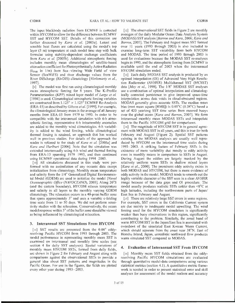
resolving Pacific HYCOM from 1993 through 2003. The model performance in representing monthly mean SST is examined on interannual and monthly time scales (see section 4 for daily SST analyses). Spatial variations of monthly mean HYCOM SSTs, formed from daily fields, are shown in Figure 2 for February and August along with comparisons against the observational SSTs to provide a general idea about SST patterns and magnitudes in the Pacific Ocean. For use in the figures, the fields are plotted every other year during 1993-2003.

[12] The observational SST fields in Figure 2 are monthly averages of the daily Modular Ocean Data Analysis System (MODAS) SST analysis [Barron and Kara, 2006; Kara and Barron, 2007]. The February and August mean SST formed over 11 years (1993 through 2003) is also included to examine long-term SST variability from both HYCOM and MODAS. The time period of 1993 through 2003 is used for evaluations because the MODAS SST re-analyses begin in 1993, and the atmospheric forcing from ECMWF is available until the end of 2003 when the interannual HYCOM simulation ended.

[13] Each daily MODAS SST analysis is produced by an optimal interpolation (OI) of Advanced Very High Resolu- tion Radiometer (AVHRR) Multichannel SST (MCSST) data [May et al, 1998]. The 1/8° MODAS SST analyses use a combination of optimal interpolation and climatologically corrected persistence to give improved space-time interpolation across data voids in cloud-obscured regions. MODAS generally gives accurate SSTs. The median mean bias (root mean square [RMS]) is 0.05°C (0.38°C) based a set of 420 yearlong SST time series from moored buoys over the global ocean [Kara and Barron, 2007]. We form interannual monthly mean MODAS SSTs and interpolate them to the Pacific HYCOM grid for comparisons.

[14] The magnitude of HYCOM SST is in general agreement with MODAS SST in all years, and this is true for both February and August (Figure 2). Spatial SST patterns existing in the MODAS analyses are usually well repro- duced by HYCOM on the interannual time scales during 1993-2003. A striking feature of February SSTs is the existence of more variability due mostly to eddy activity even in monthly means in comparison to SSTs in August. During August the eddies are largely masked by the relatively uniform warm SSTs in shallow mixed layers [Kara et al., 2000]. The prominent eddy activity exists in both MODAS and HYCOM, but there is more evidence of eddy activity in the model. MODAS tends to smooth out the highly variable character of the SST seen in a clear AVHRR image because of the data gaps and OI procedure. The model usually produces realistic SSTs colder than <0°C at high latitudes, including the northwestern parts of Japan/ East Sea in February and August.

[15] There are relatively large SST errors in some regions. For example, SST errors in the California Current system are due mainly to inadequate model upwelling. The wind forcing used for the HYCOM simulation is significantly weaker than buoy observations in this region, significantly contributing to the problem. Similarly, the zonal band of warm HYCOM SST in the Japan/East Sea is associated with overshoot of the simulated East Korean Warm Current, which should separate from the coast near 38°N. East of Honshu Island, Japan, unrealistic northward flow produces warm simulated SST compared to MODAS.

4. Evaluation of Interannual SST From HYCOM

[16] Monthly mean SST fields obtained from the eddy- resolving Pacific HYCOM simulations are evaluated through quantitative model-data comparisons using various statistical metrics (section 4.1). A quantitative metric frame- work is needed in order to present statistical error and skill analyses for assessment of the model realism and accuracy

3 of 15


ft) MODAS: February (li) IIYCOM: Kc-ln nan <r) MODAS: VII»II-I (.1) IIYCOM: August

Figure 2. Monthly mean MODAS and HYCOM SST over the North Pacific in February and August. They are shown every other year during 1993 2003, along with mean SST over all years (1993 2003). HYCOM does not assimilate any ocean data or relax to any SST data, including MODAS.

in predicting monthly mean SST from 1993 through 2003 (section 4.2). An analysis of climatological versus interannual simulations is also provided to investigate the efficacy of the atmospheric forcing in simulating the mean climatological state of the model (section 4.3).

[17] In the model-data comparisons of interannual SST, the monthly mean MODAS SST is taken as an appropriate reference (truth) because its resolution (1/8°) is close to that of the model. The resolution of MODAS is important for preserving information on front and eddy location for assimilation into high resolution dynamic forecast models. Eddies of 25 100 km in diameter cannot be adequately represented using a coarser horizontal grid. Although there are other available monthly mean interannual SST products,

they are not used in the evaluation for various reasons. For example, the monthly mean interannual NOAA SST fields, derived by a linear interpolation of the weekly optimum interpolation (OI) version 2, use in situ and satellite SST along with surface temperature in ice covered ocean regions [Reynolds et al., 2002], making it a reliable candidate for HYCOM SST validation. The existence of the ice field in the NOAA data set is also an advantage for the OGCM validation at high latitudes. However, the NOAA SST fields, mainly designed for large-scale climate studies, are produced on a 1 ° grid. This is much coarser («12 times the grid spacing) than the 0.08° Pacific HYCOM. Note that there is now a 0.25° NOAA SST product [Reynolds et al.

4 of 15

C12018 KARA ET AL.: HOW TO VALIDATE SST CI2018

2007], but our paper was written before that product became available.

[is] Another candidate interannual product is the «l/8° Pathfinder SST [Casey and Cornillon, 1999], which is based directly on satellite data. The reason for not choosing it is that, unlike the 1985-2001 Pathfinder climatological SST, there are data voids in the interannual fields due largely to cloud cover. That limits the grid by grid HYCOM-data comparisons. Therefore the monthly mean interannual MODAS SST analyses are used for assessment of HYCOM. The climatological mean Pathfinder SST will later be used for evaluating climatologically forced HYCOM simulation.

4.1. Statistical Metrics [19] Monthly mean SST time series simulated by

HYCOM are compared with those obtained from the MODAS SST analyses discussed above. The model-data comparisons are performed using the following statistical metrics: mean error (ME), root mean square (RMS) SST difference, correlation coefficient (/?) and nondimensional skill score (SS).

[20] Let Xj (i = 1,2, • • •, 12) be the set of monthly mean MODAS reference (observed) SST values from January to December, and let Yt (1 = 1, 2, • • •, 12) be the set of corresponding HYCOM_ estimates at a model grid point in a given year. Also let X (Y) and ax (oY) be the mean and standard deviations of the reference (estimate) values, respectively. Thus we have monthly mean SST time series from MODAS and HYCOM at each model grid point. The statistical relationships [e.g., Murphy, 1995] between MODAS and HYCOM SST time series are then expressed as follows:

ME ,v.

RMS £(r<-*')5 1/2

*-=!> X){Y,- Y)/(axay),

SS = R2-\R- [ay/ax)}1 - [(7 - X)/ax]2

(1)

(2)

(3)

(4)

Here, ME (i.e., annual bias) is the mean error between the HYCOM and MODAS SST values, RMS (root-mean- square) SST difference is an absolute measure of the distance between the MODAS and HYCOM time series, and R is a measure of the degree of linear association between the MODAS and HYCOM time series.

[21] The nondimensional SS given in equation (4) includes two nondimensional biases (conditional bias, 5COn<j, and unconditional bias, SUncond) which are not taken into account in the R formulation (equation (3)). In brief, 5uncond

(also called systematic bias) is a measure of the difference between the means of MODAS and HYCOM time series.

#cond is a measure of the relative amplitude of the variability in the MODAS and HYCOM SST time series or simply a bias due to differences in standard deviations of the SST time series. In equation (4) the square of correlation coefficient (R2) is equal to SS only when Z?COnd and flunCond are zero. Because these two biases are never negative, the R value can be considered a measure of "potential" skill, i.e., the skill that one can obtain by eliminating all bias from HYCOM. Note SS is 1.0 for perfect HYCOM SST simulations, and is negative for 5cond + Suncond > ^2. indicating poor simulation.

[22] The reader is cautioned that when we calculate model SST skill at high latitudes, ice poses a potential problem in the determination of R2. For example, if either MODAS or HYCOM is exactly constant for the year (e.g., all ice or no ice), then R2 is undefined. If both are constant, then it would be reasonable to set /T to 1, but this is clearly wrong if one is zero and the other is not. Since the correlation is always between the time series of MODAS and HYCOM after the mean is subtracted, one will always get 0/0 or some variant in the calculation. Adding a random term forces the correlation to be zero. In this case, we allow for the effect of a small amount of noise in both time series, that is assumed to be independent of the series. The new correlation then becomes biased. For example, in the case of ice, 5% concentration is probably insignificant so a seasonal cycle with mean = 0 and RMS = 0.05°C could be used as noise. Similarly, if one believes that 0.1 °C is not significant in the western equatorial Pacific warm pool, a seasonal cycle with a zero mean and RMS of 0.1 °C as correlated noise could be used.

[23] The procedure for allowing for the effect of noise to the time series in the correlation is as follows: Let aa be the standard deviation of the noise, with o^and cry the standard deviation of A" and Y. We then calculate /?ncw = (Raxay +

oi) I J (a^ + CJI) {(J\ + al). Note that the impact of noise

has been included without actually adding a noise to the time series. The new measure is biased, with the direction depending on the sign of R and the size of ax and ay. When ax = 0 or o> = 0, but not both, then the correlation

is 1 / \jip\lo\ + l). Thus, if <Tyis small, this approaches

1 or if ay is large relative to cra, the value approaches zero. Again, in any case the Rnev/ does not depend on the old R when <JX or aY is zero, thus always giving a result, though somewhat biased, depending on the size of aa. One can eliminate most of the bias using by a very small aa, mostly reducing the problem for calculating correlation in the case of constant MODAS and HYCOM time series.

4.2. Model-Data Comparisons in the Pacific Ocean [24] The MODAS SST provides an appropriate choice for

evaluation of the eddy-resolving Pacific HYCOM SST simulation mainly because of its resolution (1/8°). In all validation maps, white (red or blue in the case of ME) is intended to represent a tendency for successful (poor) model SST simulation for that specific statistical metric. Figure 3 presents spatial fields of ME, RMS SST difference and nondimensional SS values between monthly mean MODAS and HYCOM SST for every other year. Statistical fields based on the entire time series of monthly mean SSTs

5 of 15


(1993 2003) between HYCOM and MODAS are given in the bottom row of panels as well. Zonal averages of statistical metrics calculated at each 0.5° latitude belt are also plotted next to each panel. The shading in each zonal plot is intended to highlight the magnitude of the statistical metrics relative to 0. White in the color palette represents ME values between -0.5°C and 0.5°C, RMS < O.PC and SS > 0.95. A long-term HYCOM SST mean is also formed by averaging the interannual monthly means during 1993- 2003, e.g., the January mean SST from HYCOM is obtained by averaging all January values from 1993-2003 at each model grid point over the Pacific Ocean. This is also done for MODAS. Accordingly, in the bottom panels of Figure 3, similar statistical results are provided.

[25] The accuracy level in model SST is specified based on the derivation of the total heat flux. In particular, the total heat flux at the ocean surface (Qnct) varies with SST approximately according to ^| = (5 + 4v,) W m 2 K_l, where the first term on the right hand side comes from the longwave radiation, and the second term is due to the combined effects of the latent and sensible heat fluxes. Here, v, is the mean wind speed. If one considers a mean wind speed 10 m s_1, an SST error of even 0.5°C can lead to flux errors of more than 20 W irT2. This implies that a necessary, but insufficient condition might be the difference between model and observed SST magnitudes be less than 0.5°C for a given month.

[26] In general, annual mean SST bias between HYCOM and MODAS is small (<0.5°C) over most of Pacific Ocean (Figure 3a). This is true for all years and the 11-year mean, 1993-2003. Zonally averaged ME plots reveal that HYCOM SSTs at high northern latitudes have relatively large cold biases of wl°C in comparison to those at other latitudes. The annual mean SST along the Kuroshio pathway is well simulated by the fine resolution (0.08°) eddy- resolving HYCOM with a warm bias of «0.5°C north of the Kuroshio just east of Japan due to unrealistic northward flow in that region.

[27] SST errors («>2°C) seen in the mid-latitude interior Pacific during 1993 are partly related to an insufficient number of satellite measurements entering the MODAS SST analyses (not shown). Generally, the annual mean SST bias in the HYCOM simulations is quite low but with a warm model SST bias, typically <1°C evident in high latitudes and some mid-latitude regions in all years.

[28] The largest warm biases occur along the west coast of the U.S, in the eastern equatorial Pacific, east of Japan and in a zonal band in the Japan/East Sea, where the model subpolar front is too far north. The large biases are due in part to the atmospheric forcing and in part to deficiencies in the model, including model resolution. For example, the large warm bias just east of the Japanese Island of Honshu is due to mean northward flow where mean southward flow is observed. The boundary between the North Pacific subtropical and subpolar gyres is the subarctic front and not the Kuroshio Extension. Therefore part of western boundary current transport of the subtropical gyre must pass north of the Kuroshio Extension. The shallow and narrow straits connecting the Japan/East Sea with the North Pacific are insufficient to provide an alternate route farther to the west. Instead, this component of flow separates from the coast and reaches the subarctic front via nonlinear routes farther to the

east as observed by Levine and White [1983], Mizuno and White [1983], Niiler et al. [2003], and Isoguchi et al. [2006] and explained in modeling studies, such as those of Hurlburt et al. [1996] and Hurlburt and Metzger [1998]. These are examples of nonlinear ocean currents affecting SST.

[29] In the Japan/East Sea the simulated separation latitude of the subpolar front from the Korean coast and its pathway to the east depend on (1) the choice of atmospheric forcing product used to force the model, (2) sufficient horizontal resolution to obtain coupling between the upper ocean circulation and the eddy-driven, topographically con- strained abyssal circulation and (3) the strength of the Tsushima Warm Current along the north coast of Japan [Hogan and Hurlburt, 2005]. The strength of the upper ocean - topographic coupling is insufficient at the resolution of the 0.08° Pacific HYCOM simulation [Hogan and Hurlburt, 2000]. Along the west coast of the U.S., wind speed (solar radiation) from ECMWF is typically too low by «2ms (high by «50 W m~ ) in comparison to the buoy observations (not shown). As a result, there is insufficient upwelling of cold water along the coast, excessive solar radiation and a large warm bias in SST. SST errors due to shortwave radiation can also exist at the tropical regions [Kara et al., 2008].

[30] Similar to the annual SST bias, the RMS SST difference between HYCOM and MODAS calculated over the seasonal cycle (see section 4.1) is generally small (<0.5°C) over much of the Pacific Ocean in all years (Figure 3b). Large RMS SST differences (e.g., 2°C or so) are noted in the northwestern and eastern equatorial Pacific. Zonally averaged RMS SST plots further confirm large errors at high latitudes.

[31] Figure 3c presents a striking feature of the model evaluation. For example, nondimensional SS maps reveal relatively low SST skill from HYCOM in the equatorial Pacific in comparison to the other parts of Pacific, while RMS SST differences are very small in the same region. Similarly, relatively large RMS SST differences exist in the northwestern Pacific at high latitudes but SST skill is usually quite high. It is therefore important to note that using RMS SST difference by itself may result in misleading information about the model evaluation.

[32] The nondimensional SS includes correlation, conditional and unconditional biases (Figure 4), thus it is expected to provide better information about the source of the model bias. The low model skill in the equatorial Pacific is due mainly to the mismatch between means of HYCOM and MODAS SST, which, though small, is large compared to the standard deviation of the data (ax in equation (4)) making flunCond 'arge in that region. Relatively low R (<0.8 in some areas) is a secondary contribution to SST skill. HYCOM captures variations in monthly mean SST very well because 5cond is generally <0.1 in the 11 -year mean, confirming that the model reproduces SST standard deviation annually as in the MODAS SST fields. This is true not only for the equatorial regions but also for most of the Pacific in all years. This is also evident from the basin- averaged statistics (Table 1), showing large 5uncond values in comparison to ficond values in all years.

[33] An interesting point of Figure 4 is that the model gives realistic SST simulations along the Kuroshio pathway. This is an important result because the simulation of the

6 of 15


(a) Mi>nn error ( C (b) RMS tlilF. ( C) (»•) Skill scor<

O -* M W » Ul O O — — ro ro w o -* to OOOOOOOOO b t» b in b w b bee b-»k>o»*«uid*;-jai

Figure 3. Annual maps of (a) mean error (ME), (b) RMS SST difference, and (c) SST skill score (SS) between HYCOM and MOD AS given for every other year from 1993 through 2003. Statistical metrics are described in section 4.1. Statistics over all years (1993 2003) are shown in the last row. Zonal averages are provided next to each panel.

Kuroshio pathway is generally not realistic using coarse resolution OGCMs, leading to pathway errors and advection that is too weak [e.g., Hurlburt and Hogan, 2000]. For example, Kara et al. [2003] found that a coarse resolution (1/2°) OGCM which has only 6 layers in the vertical was unable to simulate accurate SSTs along the Kuroshio pathway. Interannual simulations performed with the fine resolution (0.08°) eddy-resolving HYCOM clearly demon- strate that it is possible to accurately simulate SST in the Kuroshio pathway as evidenced by very large SS values in all years (Figure 3c). This is in part accomplished by using 6-h atmospheric forcing from ECMWF with the use of bulk parameterizations for sensible and heat fluxes calculated at each model time step.

[34] The model skill in simulating monthly mean SST is relatively high in some parts of the northwestern and northeastern Pacific. This contradicts large RMS differences, a misleading indication of the model performance in simulating SST in these regions. Because SCOnd and 5Uncond are very small and R is close to 1 in these regions, SS maps reveal skillful SST simulations from HYCOM. Since SST standard deviations are very different at the equator (small SST variability) and high latitudes (relatively large SST variability), nondimensional SS provides an independent comparison between the two regions by taking all components of possible biases into account in the model evaluation. This topic is discussed further in section 5. Overall, HYCOM SST simulations yield zonally averaged

7 of 15


(a) Correlalloi (hi Conditional bU

\ ^hr^:

. *«^K^

i

:) I i MI >ii(|il iun.il bia>

Jl \

IL

>*" v v * • » "'

• -V; 8

Figure 4. Same as Figure 3 but for (a) correlation coefficient (R), (b) conditional Bcond, and (c) unconditional fiunCond biases between HYCOM and MODAS SST. The white color represents R values of >0.95 and flcond or Bunconii of <0.05.

R values > 0.9 at all latitude belts except for equatorial Pacific. The largest 5con<j and fiunCond are seen in the equatorial Pacific. While this bias is not reflected in R, it causes SS < 0.1 in some regions of the equatorial Pacific.

4.3. ( limatological Versus Interannual Simulations [35] In this section, we seek answers to a particular

question, "what is the accuracy of climatologically forced simulations with respect to the climatology of the interannually forced simulations presented in section 3"? The answer to this question would reveal whether or not the monthly climatological atmospheric forcing produces a monthly and annual mean climatological ocean state that is comparable in realism and accuracy to a interannual simulation, a significant issue for long-term simulations.

[36] For the climatological model simulation, the initial assumption is that monthly mean climatological atmospheric forcing (with 6-h wind anomalies, but no other atmospheric forcing anomalies) would give the monthly mean climatological ocean state. The validity of this assumption is largely confirmed by comparing the monthly mean of long- term mean SSTs (i.e., 1993-2003) from the interannually forced HYCOM simulations with those from the climatologically forced simulation (Figure 5). However, there are some noteworthy exceptions, e.g., more (less) accurate results from the interannual simulation in the subtropical (subpolar) gyre. The interannual simulation generally gives slightly better SSTs at most latitude bands (Figure 6), with much higher correlation and skill score near the equator. In part, these differences could be due to the different time

8 of 15


Table 1. Basin-Averaged SST Validation Statistics" Between HYCOM and MODAS During 1993 2003

Year ME (°C) RMS (°C) R SS

1993 0.32 0.88 0.08 0.28 0.84 0.36 1994 0.06 0.79 0.08 0.23 0.83 0.41 1995 0.27 0.80 0.09 0.20 0.86 0.46 1996 0.09 0.77 0.07 0.23 0.85 0.45 1997 0.10 0.65 0.05 0.14 0.88 0.58 1998 0.21 0.86 0.06 0.21 0.84 0.46 1999 0.26 0.92 0.05 0.34 0.85 0.35 2000 0.21 0.77 0.05 0.18 0.87 0.54 2001 0.08 0.79 0.04 0.20 0.87 0.53 2002 0.00 0.78 0.04 0.29 0.86 0.43 2003 0.(15 0.69 0.05 0.22 0.88 0.52

"All analyses arc based on monthly mean values (i.e., monthly mean HYCOM SST versus monthly mean MODAS SST) at each model grid point, and basin-averaged means arc calculated over the entire Pacific HYCOM domain. An SS value of 1 indicates perfect HYCOM simulation with respect to MODAS SST.

covered regions even though it only includes a simple thermodynamic ice model. There are also model errors due to the model circulation (e.g., in the Japan/East Sea) and atmospheric forcing (e.g., off the California coast), which can also contribute to inaccurate simulation of SST.

5. HYCOM Evaluation Using Daily Buoy SST Time Series

[41] The variety of TAO, NDBC and Canadian moored buoy locations (see Figure 1) provides an excellent source for the HYCOM SST model-data comparisons for the interannual simulation. This is valid even though the spatial sampling of buoys is sparse. HYCOM is not only designed for open ocean studies but also coastal processes, an important feature of the hybrid coordinate model approach.

periods used in forming the climatological forcing and the mean from the interannual simulation.

[37] If the climatologically and interannually forced model simulations gave significantly different results, then we would have to re-assess our strategy of using monthly winds with 6-h anomalies and monthly mean thermal forcing. One reason why wind anomalies are enough is that they are sufficient to allow for the bulk parameterization to give 6-h variability in the total heat flux. That is clearly evident from the accuracy of SST validation statistics.

[38] The same validation procedure for both HYCOM simulations is repeated using the 4-km Pathfinder SST climatology (Figures 5c and 5d). This data set was formed using the same techniques as that of Casey and Cornillon [1999] but on the newer «4 km data (rather than «9 km) over 1985-2001. Zonally averaged statistical results remain almost the same when validating HYCOM against the Pathfinder SST climatology (Figure 7), in comparison to those shown in Figure 6 except that the annual mean bias is slightly increased (0.09°C to 0.23°C for the climatologically forced simulation and 0.15°C to 0.29°C for the interannual simulation).

[39] HYCOM SST errors with respect to the MODAS climatology are generally large in high northern latitudes (Figure 5). The reason is that there is no specific treatment for the existence of ice in MODAS SSTs, i.e., SSTs are just filled from the nearest grid point. However, the model errors are significantly reduced in these regions when the Path- finder SST climatology is used for the validation. The reason is that we modified the Pathfinder climatology so that the SST includes the ice concentration climatology from NO A A to decide if a data void should be treated as ice. This procedure was not originally applied to MODAS because it is a daily data set.

[40] The original Pathfinder SST climatology includes neither a specific ice climatology nor a clear separation between ice values and a data void. Even though the Pathfinder climatology (unlike the interannual Pathfinder SST data set) is gap filled, there are places, such as parts of the Arctic and inland waters, where the Pathfinder SST are not very reliable. When HYCOM is validated against the new climatology that we produced for ice treatment, HYCOM does in fact adequately simulate SST in ice-

i..i \1h : ( i IIMOU ,~ \IOI>\S {l.i SV ini'UM v- \lt>l>\s

. I""

I. I ME I ('): HYCOM va l\.il,l..i,l.. hi I SSi 111 COM n l'..i l.n.,,1. i

V

V

0zs

N U » W

Figure 5. Comparisons of the climatologically and interannually forced HYCOM simulations with respect to the MODAS SST climatology formed over 1993-2003. For the climatologically forced HYCOM simulation, monthly mean SSTs are formed over the 7 years of the simulation, and for the interannually forced HYCOM simulation, the long-term monthly mean SST (11 years) is formed during 1993-2003 to compare with MODAS SST climatology. Panels in Figures 5c and 5d are the same as Figures 5a and 5b, but SST is validated against the 4-km Pathfinder climatology.

9 of 15


— Climatologically-forecd Inter-annual simulation

0.0

-0.4 1.0

a: 0.9 0.8

0.7 0.3

|0.2 00 0.1

0.0 0.9

|o.6

on 0.3

0.0

- 0.04 - 0.02

_z^^_ L S ^—*^. r^\}

ION 20N 30N 40N SON 60N

«3 km which is smaller than the grid resolution of HYCOM. This is a drift circle diameter within which the buoy moves. For consistency, in extracting HYCOM SSTs at buoy locations we calculated the average position based on the historical values of latitude and longitude.

[44] There are 59 NDBC buoys, 60 TAO buoys and 16 Canadian buoys reporting multiyear SST time series as used in this study. Daily averages of SST from all available buoys are formed for HYCOM SST evaluation over the time period 1990-2003 rather than the time period of 1993- 2003 used earlier. The latter was used because MODAS SST is available starting from 1993 rather than 1990. In the analysis no temporal smoothing is applied to the original SSTs from buoys, but small data gaps are filled by linear interpolation. Time series with more than a few small gaps within a year (>1 month) are excluded. The daily SST time series give information on a whole range of time scales from >1 day to interannual, a desired feature for comprehensive model-data comparisons. Daily averaged HYCOM SST time series for each year are also extracted at the same buoy locations. For that purpose we used the historical buoy positions. The current version of HYCOM does not simulate the diurnal cycle, thereby daily snapshots of SST are obtained from the model simulation. The model is sampled everywhere once a day at 00Z (midnight UTC). Since the thermal atmospheric forcing has a one day running mean applied to it, diurnal effects are minimized in the model and sub-daily sampling is not needed.

Figure 6. Zonally averaged statistical comparisons between monthly mean HYCOM and MODAS SSTs when the model was run using the climatological 6-h wind and thermal forcing from the ECMWF and interannually from 1993 through 2003. Zonal averaging is performed for each 0.5° latitude belt. Basin-averaged values for each statistical metric (calculated for the Pacific HYCOM domain) are given inside each panel.

Thus we further perform SST evaluations at coastal and open ocean locations.

[42] Daily averaged SST time series from all moored buoys are used for HYCOM SST evaluation. The TAO moorings are deployed every 2° -3° of latitude between 8°N and 8°S along lines that are separated by 10°-15° of longitude (http://www.pmel.noaa.gov/tao/index.shtml). SST time series from the NDBC moorings are available at many locations in the Pacific Ocean: some distance off the U.S. coasts (California, northeast Pacific), eastern Alaskan coast and the Hawaiian islands (http://www.nodc.noaa.gov/ BUOY/buoy.html). The Environmental Monitoring Divi- sion of Canada also maintains a network of moored buoys along the coast of Canada since the 1990s (http://www. atl.ec.gc.ca/msc/em/marine_buoys.html).

[43] All buoys report hourly SST measured at a nominal depth of wl m below the sea surface, and daily averages are formed for HYCOM-data comparisons following quality control checks and the filling of short data voids (<30 days) by a linear interpolation. Buoy locations can also change by a few km whenever a mooring is recovered and a new one deployed. This change may happen over the course of a few days to a week depending on the current regime by up to

Climatologically-forced Inter-annual simulation

Figure 7. Same as Figure 6 but HYCOM is validated against the 4-km Pathfinder SST climatology.

10 of 15

CI2018 KARA ET AL.: HOW TO VALIDATE SST C12018

(23°N, 162°W) SST HYCOM SST

Jan Feb Mar Apr May Jun Jul Aug Sep Oct Nov Dec

Figure 8. Daily averaged SST at 23°N, 162°W located near an island of northwestern Hawaii from an NDBC buoy (thin solid line) and modeled SST (thick solid line) from the 0.08° Pacific HYCOM simulation. The approximate buoy location is at 23.40°N, 162.25°W. Missing buoy SSTs near the end of 1997 are filled using a linear interpolation.

[45] One challenge for the model evaluation is how best to compare intermittent time series of different lengths and covering different time intervals, while allowing interannual comparison of verification statistics at the same location and comparison of statistics at different locations over the same time interval. As a result, the time series were divided into 1 year segments with daily averaged values. This approach also facilitates later inter-model comparisons.

[46] Using three buoys, we first illustrate the model assessment analysis between buoy and HYCOM SST time series, a procedure used for all the buoys. The three buoys are located in different regions of the Pacific Ocean. They are selected to represent equatorial, tropical and high latitudes. Yearly SST time series comparisons performed for selected years (1992, 1995, 1997, and 2002) are shown for the NDBC buoy (Figure 8), a TAO buoy (Figure 9), and a Canadian buoy (Figure 10). There is no specific reason for the selection of these particular years. The seasonal cycle of SST is prominent in the NDBC and Canadian buoy data, but not at the TAO buoy. This is generally true in all years. Atmospherically forced HYCOM is able to simulate daily

SST well, including its interannual variations for all buoys in all years.

[47] Statistical model-data comparisons between the yearlong HYCOM and buoy SST time series at the three buoy locations give a quantitative assessment of errors in the HYCOM simulation (Table 2). Results are provided for the years when yearlong daily buoy SST time series data were available, although we presented daily SST time series only for 4 years (1992, 1995, 1997, and 2002), for simplicity. In the time series comparisons n is equal to 365 (or 366 for leap years) for each yearlong data at a given buoy location (see section 4a). The ability of HYCOM to predict daily SST on interannual time scales is encouraging, in that there is positive skill in all years except for 1994 at (00°N, 110°W). The skill values are very high (close to 1) in a majority of years, a feature particularly evident for the NDBC and Canadian buoys. Annual mean SST biases are generally within 1°C between the HYCOM simulated SSTs and buoy SSTs. The model is able to the capture the phase of SST variability quite well, i.e., R is generally high. All these statistical comparisons suggest that HYCOM is able to simulate SST with similar errors for nearly all years. Such

(00°N, 110°W) SST HYCOM SST

30 28 26 24 22

- |(D) lWD |

"?^y|lvw^^yvv fcaU-l j f

30 28

VI 26 21

24§ 22


Figure 9. Same as Figure 8 but daily averaged SST from a TAO buoy (thin solid line) at 00°N, 110°W located in the equatorial Pacific and modeled SST (thick solid line) from the 0.08° Pacific HYCOM simulation. The approximate buoy location is at 0.05°N, 109.94°W.

11 of 15


(51°N, 130°W)SST HYCOM SST


Figure 10. Same as Figure 8 but daily averaged SST from a Canadian buoy (thin solid line) at 51°N, 162°W located near the Canada coast and modeled SST (thick solid line) from the 0.08° Pacific HYCOM simulation. The approximate buoy location is at 50.88°N, 129.91°W.

accuracy also facilitates accurate SST in data-assimilative versions of the model and in model SST forecasting, capabilities already running in real time using 0.08° global HYCOM (http://www7320.nrlssc.navy.mil/projects.php).

[48] Using only one statistical metric does not provide enough information about the model performance. For example, at (23°N, 162°W) the RMS SST difference of 0.90°C in 1992 is smaller than 1.29°C at (00°N, 110°W) during the same year. This certainly suggests that the HYCOM SST simulation at (00°N, 110°W) is worse than at (23°N, 162°W). However, an examination of the nondimensional SS reveals that the SS value (0.74) at the second location is higher than at the first one (0.66) in 1992. Thus HYCOM SST simulation at (00°N, 110°W) is in fact better than the one at (23°N, 162°W). This is due to the fact that the standard deviation of the buoy SSTs are quite different at these two locations (1.54°C versus 2.52°C). This result illustrates the importance of using the skill score in validating OGCM performance, especially when assessing model performance at different locations where SST seasonal cycles are quite different.

[49] Some SST errors in the coastal regions (e.g., in the U.S. west coast) can be attributed to the coarse resolution

ECMWF forcing used for the HYCOM simulations. A creeping sea-fill, which can be applied to scalar atmospheric variables, could help in reducing such bias. Kara et al. [2007] discuss the details of this methodology and its effects in 0.04° HYCOM simulations of the Black Sea. The Pacific HYCOM simulations were performed before the creeping sea-fill methodology had been developed, and they were not repeated with the sea-filled atmospheric forcing due to computational expense.

[50] Model-data comparisons like those performed at (23°N, 162°W), (00°N, 110°W) and (51°N, 130°W) are applied to all the buoys. Using available daily SST time series from all buoys for each year, statistics are calculated in a manner similar to that for the three buoys in Table 2. The main purpose is to assess overall HYCOM performance in simulating SST over the period 1990 2003. The NDBC, TAO and Canadian buoys yield a total of 804 yearlong time series over this period and 804 corresponding values of ME, RMS, R and SS, which are used in further analysis of

Table 2. Statistical Verification8 of Daily SST Between HYCOM

and a Buoy Representing Each Buoy Setb

Statistics (n = I year) Standard Deviation

Year RMS (°C) ME (°C) R SS Buoy (°C) HYCOM (°C)

NDBC Buoy (23°N. 162°W) 1990 1991 1992 1993 1995 1997 1998 1999 2000 2001 2002

1990 1991 1992 1993 1994 1995 1997 1999 2000 2001 2002

1990 1992 1993 1995 1996 1997 1998 2000 2001 2002

0.59 1.04 0.90 0.83 0.61 0.88 0.56 0.55 0.43 0.43 0.43

1.49 1.01 1.29 1.35 1.37 1.60 0.82 2.19 1.54 1.42 0.81

1.07 1.26 1.76 0.98 1.18 0.93 0.90 0.85 0.85 0.90

-0.31 -0.77 -0.64 -0.67 0.02 -0.73 -0.21 -0.25 -0.07 -0.10 -0.10

0.94 0.90 0.91 0.95 0.89 0.96 0.90 0.89 0.94 0.92 0.96

0.84 0.56 0.66 0.71 0.79 0.73 0.77 0.74 0.87 0.83 0.90

1.48 1.58 1.54 1.55 1.35 1.72 1.17 1.06 1.18 1.05 1.38

TAO Buoy (0(fN, HCfW) 1.14 0.53 0.76 0.69 0.01 1.14 -0.30 1.92 1.23 1.14 0.11

0.82 0.83 0.93 0.78 0.25 0.85 0.85 0.89 0.87 0.91 0.80

0.19 0.54 0.74 0.47 -0.25 0.31 0.68 0.02 0.30 0.49 0.63

1.65 1.49 2.52 1.86 1.22 1.92 1.45 2.21 1.84 1.99 1.33

Canadian Buoy (5l"N. li(fW) 0.88 1.07 1.53 0.75 1.00 0.51 0.61 0.52 0.69 0.58

0.98 0.95 0.94 0.97 0.97 0.97 0.95 0.97 0.98 0.98

0.88 0.65 0.50 0.86 0.76 0.90 0.83 0.89 0.87 0.89

3.12 2.13 2.49 2.58 2.40 2.95 2.20 2.53 2.34 2.76

1.31 1.40 1.37 1.40 1.32 1.59 1.09 1.05 1.03 1.06 1.42

1.29 1.44 1.90 1.54 0.99 2.09 1.26 1.79 1.53 1.84 1.23

2.91 2.02 2.50 2.43 2.43 2.64 2.08 2.35 2.22 2.39

"The statistical results are calculated based on 365 daily values (366 for leap years, i.e., 1992, 1996, and 2000). A skill score value of <0 indicates a poor model simulation.

bRcsults arc shown for 00°N, I10°W in the eastern equatorial Pacific Ocean, a Canadian buoy at 51°N, I30°W near the coast, and an NDBC buoy at (23°N, 162°W) near Hawaii.

12 of 15


(a) Mean SST error

•C °G °G °G »0 »0 »0 °G «G oO oO «G & & J> J J> as> OV0 an? „*>* 0v> >» J> <0 «0 w

(b) RMS SST difference

f c0-° C-° ttvO ^ ô ô 0vO .* f ^\^^ S**<> T? V

oO <>G ô °o °o °o °o °o °o °c °o

,A* *' <p OP v>v .«• >° «.v°

(c) SST correlation (d) SST skill score

»> 0> «£ ^ *> <£ $ 0* «? \* <? J> <*y tf »* *> & $ *?> «? s<? .v° «f Nv° «,* b<P Av° ^ c'P

0> o> ©•' o!" 0~ <S- ©• 0- 0^ * 0> o> <£ ** v£ 0* 0^ 0* «? Class intervals Class intervals

Figure 11. Histograms of the total number of yearlong buoy time series per class interval for each statistical metric based on the daily comparisons between HYCOM and buoy SSTs during 1990 2003. As mentioned in the text, a given buoy can have multiple yearlong daily SST time series during 1990 2003, and here we represent each yearlong time series as one count per buoy. Of the 804 yearlong time series from all buoys, a total of 220 come from 59 NDBC buoys, 457 from 60 TAO buoys, and 127 from 16 Canadian buoys. Nearly half of the RMS SST differences (377 out of 804 buoys) lie between 0.5°C and 1.0°C. Since any negative SS is considered as poor simulation, all SS values <0 are represented by one histogram bar in the plot, a total of 277 out of the 804 buoy time series.

HYCOM performance. Of these, 380 have ME values that lie between -0.5°C and 0.5°C, 206 buoys with -0.5°C < ME < 0°C, and 174 buoys with 0°C < ME < 0.5°C (Figure 11).

[51] Cumulative frequency is another way of expressing the number of ME, RMS, R and SS values that lie above (or below) a particular value (Figure 12). Error statistics based on comparing the 804 daily SST buoy time series with the HYCOM simulation over the time frame 1990 2003 give a median warm HYCOM SST bias of 0.23°C, RMS SST difference of 0.83°C, R of 0.86 and SS of 0.40 (Table 3). Median SST standard deviations for the buoys (1.15°C) and HYCOM (1.10°C) are very close. Consistent with the monthly mean SST evaluation (see Figure 3c), daily HYCOM SST simulations are least skillful in the equatorial regions as evident from the median statistics. Clearly, the lowest median SS of 0.28 (but still positive) for TAO buoys is significantly smaller than those for the NDBC (0.54) and

Canadian (0.77) buoys, mainly due to the relative amplitude of the seasonal cycle. Although TAO buoys have the lowest median RMS SST difference of 0.68°C and ME of -0.10°C, the nondimensional SS helps detect HYCOM deficiencies in simulating daily SST within the equatorial Pacific.

6. Summary and Conclusions

[52] In this study, eddy-resolving (0.08°) climatoiogical and interannual HYCOM simulations of the Pacific Ocean north of 20°S were described, and a metric evaluation of simulated SSTs was presented. The metric evaluation reveals that HYCOM has the ability to replicate past SST events in the interannual simulation, and both the climatoiogical and interannual simulations yield nearly the same monthly and annual mean climatologies in good agreement with observations. This is a critical requirement for OGCM studies that are developed for both short- and long-term

13 of 15


(a) Mean SST error MX)

» 70° O 600 3 OQ 500

o ha I E 3 z

4(X)

«X)

200

100

~t

j j

4.0 -3.0 -2.0 -1.0 0.0 1.0 2.0 3.0 4.0 5.

800-

(b) RMS SST difference

700-

600-

500 ! 1

400-

300

200

100-

0 ' i i

(°C) 0 0.0 0.5 1.0 1.5 2.0 2.5 3.0 3.5 4.0 4.5 5.0

(°C)

o 3

CQ

I E 3 z

(c) SST correlation 800 -

600-

1

500 -

400

!

300-

200-

100

0 i 1

(d) SST skill score

-0.2 -0.1 0.0 0.1 0.2 0.3 0.4 0.5 0.6 0.7 0.8 0.9 1 .0 0.1 0.2 0.3 0.4 0.5 0.6 0.7 0.8 0.9 1.

Figure 12. The cumulative frequencies of HYCOM SST statistics (see Figure 11). The cumulative frequency is calculated by progressively summing the percentage of the cumulative frequency within each interval, providing an easy way to illustrate the effectiveness of HYCOM in predicting daily SST during 1990 2003.

climate studies. When the model climatology was validated against satellite-based SST products over the seasonal cycle during the 1993-2003 time frame, the interannual HYCOM simulation gave a slightly lower basin-averaged RMS SST difference of 0.6°C than the value of 0.7°C obtained from the climatologically forced simulation. This confirms our strategy of using monthly winds with 6-h anomalies and monthly mean thermal forcing to obtain realistic SSTs.

[53] In comparison to the satellite-based MODAS SST, the nondimensional skill score maps clearly show that HYCOM is able to simulate SST well in the Pacific since the two nondimensional biases are generally (<0.1) in most regions except the equatorial Pacific. High correlation values close to 1 indicate that the model is able to reproduce the SST seasonal cycle in good agreement with MODAS SST over most of the Pacific Ocean. This is true in all years during the 1993-2003 time frame, and in the 1993 2003 mean. Because SST variability in the equatorial Pacific warm pool is so small (i.e., small standard deviation) the RMS SST differences are also small. However, skill score revealed HYCOM deficiencies in predicting daily and monthly mean SST in this region. Because of the very small amplitude of the seasonal cycle and the SST variability in this region, higher accuracy in (1) the atmospheric forcing (including salinity forcing) and in (2) the numerical model are needed to accurately represent this variability than is required in most other regions. The model also gives

poor performance in representing the SST seasonal cycle at high northern latitudes where ice effects are of importance.

[54] One of other major goals of this study is to present a evaluation procedure at many individual buoy locations using various statistical metrics. Availability of the well- organized and maintained historical SST time series from TAO, NDBC and Canadian buoys provided a unique opportunity to determine the success and shortcomings of HYCOM SST simulations in different regions of the global ocean during the 14-year period (1990-2003). Thus we examine the weakness and strength of an atmospherically forced OGCM in simulating daily SST and its interannual variability at the buoy locations in a systematic way, which

Table 3. Median Error Statistics* for Yearlong Daily Time Seriesb

During 1990-2003

Buoy Total RMS ME "BUOY "HYCOM SST Buoys fq (°C) R SS (°C) (°C)

Canadian 127 1.21 0.86 0.97 0.77 2.58 2.61 NDBC 220 1.46 1.18 0.92 0.54 1.80 2.11 TAO 457 0.68 -0.10 0.77 0.28 0.75 0.66 All 804 0.83 0.23 0.86 0.40 1.15 1.10

"Median values of SST statistics for Canadian. NDBC, and TAO buoys arc shown separately.

'There arc 127 yearlong daily SST (127 x 365 days) time scries from Canadian buoys, 220 from NDBC buoys, and 457 from TAO buoys that arc used for model-data comparisons. For leap years, n = 366 rather than 365.

14 of 15


could also easily be applied to other OGCMs. The results reveal that HYCOM is able to reproduce SST in consistent with buoy measurements. In particular, based on the 804 yearlong daily SST buoy time series HYCOM gives a median warm SST bias of 0.23°C and an RMS SST difference of 0.83°C over the time frame 1990-2003.

[55] Finally, HYCOM as presented in this paper is a part of the U.S. Global Ocean Data Assimilation Experiment (GODAE), and its development toward operational use. Results from the data assimilative version of model configured for the global ocean are available online at http:// www.hycom.org/, including snapshots, animations and forecast verification statistics for many zoom regions, not only for SST but also for other variables, such as sea surface height (SSH) and surface currents. The assimilative version of the model is also running in real time (http://www7320. nrlssc.navy.mil/projects.php).

[56] Acknowledgments. This research was funded by the Office of Naval Research (ONR) under program clement 601153N as part of the NRL 6.1 project Global Remote Littoral Forcing via Deep-Water Pathways and the 6.2 project Hybrid Coordinate Ocean Model and Advanced Data Assimilation. Valuable discussions with C. Barron (NRL) regarding the MODAS SST rcanalysis arc greatly appreciated. We would like to thank G. Halliwell and R. Block for their contributions in the model development. Additional thanks go to M. McPhadcn of the TAO project office, Environ- mental Monitoring Division of Canada and NODC for providing buoy SST for the model validation. The reviewers provided helpful comments which improved the quality of this paper. The HYCOM simulations were performed on an IBM SP POWER3 at the Army Research Laboratory, Aberdeen, Maryland, and on a SGI Origin 3900 at the Aeronautical Systems Center, Wright-Peterson Air Force Base, Ohio, using grants of high-performance computer time from the Department of Defense High Performance Computing Modernization Program. This is contribution NRL/JA/7320/08/8192 and has been approved for public release.

References Barron, C. N„ and A. B. Kara (2006), Satellite-based daily SSTs over the

global ocean, Geophys. Res. Lett., 33, L15603, doi:10.1029/ 2006GL026356.

Blcck, R. (2002), An oceanic general circulation model framed in hybrid isopyenic-Cartesian coordinates. Ocean Modeli, 4, 55-88.

Casey, K. S., and P. Cornillon (1999), A comparison of satellite and in situ based sea surface temperature climatologies, J. Clim., 12, 1848-1863.

Gibson, J. K., P. Kallbcrg, S. Uppala, A. Hernandez, A. Nomura, and E. Serrano (1999), ECMWF Re-Analysis Project Report Series. I: ERA Description (Version 2), 74 pp. (Available from ECMWF, Shinfield Park, Reading, UK.)

Hogan, P. J., and H. E. Hurlburt (2000), Impact of upper-topographical coupling and isopycnal outcropping in Japan/East Sea models with 1/8° to 1/64° resolution, J. Phys. Oceanogr., 30, 2535-2561.

Hogan. P. J., and H. E. Hurlburt (2005), Sensitivity of simulated circulation dynamics to the choice of surface wind forcing in the Japan/East Sea, Deep Sea Res.. Part II, 52, 1464-1489.

Hurlburt, H. E., and P. J. Hogan (2000), Impact of 1/8° to 1/64° resolution on Gulf Stream model-data comparisons in basin-scale subtropical Atlan- tic Ocean models, D\n Atmos Oceans, 32, 283-329.

Hurlburt, H. E., and E. J. Metzgcr (1998), Bifurcation of the Kuroshio extension at the Shatsky Rise, J. Geophys. Res., 103, 7549-7566.

Hurlburt, H. E„ A. J. Wallcraft, W. J. Schmitz Jr., P. J. Hogan, and E. J. Metzgcr (1996), Dynamics of the Kuroshio/Oyashio current system using eddy-resolving models of the North Pacific Ocean, J. Geophys. Res., 101, 941-976.

Hurlburt, H. E„ E. P. Chassignct, J. A. Cummings, A. B. Kara, E. J. Metzgcr, J. F. Shrivcr, O. M. Smcdstad, A. J. Wallcraft, and C. N. Barron (2008), Eddy-resolving global ocean prediction, in Ocean Modeling in an Eddying Regime, Geophys. Monogr. Ser, vol. 177, edited by M. Hccht and H. Hasumi, pp. 353-381, AGU, Washington, D. C.

Isoguchi, O., H. Kawamura, and E. Oka (2006), Quasi-stationary jets trans- porting surface warm waters across the transition zone between the sub-

tropical and the subarctic gyres in the North Pacific, J. Geophys. Res.. Ill, C10003, doi:10.l029/2005JC003402.

Kara, A. B., and C. N. Barron (2007), Fine-resolution satellite-based daily sea surface temperatures over the global ocean, J. Geophys. Res., 112, C05O41, doi: 10.1029/2006JC004021.

Kara, A. B., and H. E. Hurlburt (2006), Daily inter-annual simulations of SST and MLD using atmosphcrically-forccd OGCMs: Model evaluation in comparison to buoy time scries, J. Mar. Syst., 62, 95- 119.

Kara, A. B., P. A. Rochford, and H. E. Hurlburt (2000), Mixed layer depth variability and barrier layer formation over the North Pacific Ocean, / Geophys. Res., 105, 16,783-16,801.

Kara, A. B., A. J. Wallcraft, and H. E. Hurlburt (2003), Climatological SST and MLD simulations from NLOM with an embedded mixed layer, J. Atmos. Ocean. Techno!., 20, 1616-1632.

Kara, A. B„ A. J. Wallcraft, and H. E. Hurlburt (2005a), Sea surface temperature sensitivity to water turbidity from simulations of the turbid Black Sea using HYCOM, J. Phys. Oceanogr, 35, 33-54.

Kara, A. B., H. E. Hurlburt, and A. J. Wallcraft (2005b), Stability-dependent exchange coefficients for air-sea fluxes, J. Atmos. Ocean. Techno!, 22, 1080-1094.

Kara, A. B., A. J. Wallcraft, and H. E. Hurlburt (2007), Land contamination of atmospheric forcing for ocean models near land-sea boundaries. J. Phys. Oceanogr, 37, 803-818.

Kara, A. B., A. J. Wallcraft, P. J. Martin, and E. P. Chassignct (2008), Performance of mixed layer models in simulating SST in the equatorial Pacific Ocean, J. Geophys. Res., 113, C02020, doi:10.l029/ 2O07JCO04250.

Large, W. G., J. C. McWilliams, and S. C. Doncy (1994), Oceanic vertical mixing: A review and a model with a nonlocal boundary layer parameterization. Rev. Geophys., 32, 363-403.

Lau, N.-C, and M. J. Nath (2001), Impact of ENSO on SST variability in the North Pacific and North Atlantic: Seasonal dependence and role of cxtratropical sea-air coupling, J. Clim., 14, 2846-2866.

Lcvinc, E. R., and W. B. White (1983), Bathymctric influences upon the character of North Pacific fronts, J. Geophys. Res., 88, 9617-9625.

May, D. A., M. M. Parmctcr, D. S. Olszewski, and B. D. McKcnzic (1998), Operational processing of satellite sea surface temperature retrievals at the Naval Occanographic Office, Bull. Am. Meteorol. Soc, 79, 397-407.

McPhaden, M. J. (1995), The Tropical Atmosphere Ocean (TAO) array is completed, Bull. Am. Meteorol. Soc., 76, 739-741.

Mizuno, K, and W. B. White (1983), Annual and intcrannual variability in the Kuroshio Current system, J. Phys. Oceanogr., 13, 1847- 1867.

Murphy, A. H. (1995), The coefficients of correlation and determination as measures of performance in forecast verification, Weather Forecasting, 10, 681 -688.

Naval Occanographic Office (NAVOCEANO) (2003), Database Descrip- tion/or the Generalized Digital Environmental Model (GDEM-V) Version 3.0. OAML-DBD-72, 34 pp.. Naval Oceanogr. Off, Stcnnis Space Center, Miss.

Niilcr, P. P., N. A. Maximcnko, G. G. Pantclccv, T. Yamagata, and D. B. Olson (2003), Near-surface dynamical structure of the Kuroshio Exten- sion, J. Geophys. Res., I08(Cb), 3193, doi:10.l029/2002JC001461.

Peng, S. L., W. A. Robinson, and M. P. Hoerling (1997), The modeled atmospheric response to midlatitudc SST anomalies and its dependence on background circulation states, J. Clim., 10, 971-987.

Reynolds, R. W., N. A. Rayner, T. M. Smith, and D. C. Stokes (2002). An improved in-situ and satellite SST analysis for climate, J. Clim., 15, 1609-1625.

Reynolds, R. W., T. M. Smith, C. Liu, D. B. Chclton, K. S. Casey, and M. G. Schlax (2007), Daily high-resolution blended analyses for sea surface temperature, J. Clim., 20, 5473-5496.

Schneider, N., A. J. Miller, and D. W. Pierce (2002), Anatomy of North Pacific decadal variability, J. Clim., 15, 586-605.

Trcnbcrth, K. E., G. W. Branstator, D. Karoly, A. Kumar, N.-C. Lau, and C. Ropclcwski (1998), Progress during TOGA in understanding and modeling global tclcconncctions associated with tropical sea surface temperature,/ Geophys. Res., 103, 14,291-14,324.

VSrosmarty, C. J., K. Sharma, B. M. Fckctc, A. H. Copcland, J. Holdcn, J. Marble, and J. A. Lough (1997), The storage and aging of continental runoff in large reservoir systems of the world, Ambio, 26, 210-219.

E. P. Chassignct, Center for Ocean-Atmospheric Prediction Studies and Department of Oceanography, Florida State University, 2035 E. Dirac Drive, Suitc-200 Johnson Bldg., Tallahassee, FL 32310, USA.

H. E. Hurlburt, A. B. Kara, E. J. Metzger and A. J. Wallcraft, Oceanography Division, Naval Research Laboratory, Code 7320, Building 1009, Stennis Space Center, MS 39529, USA. ([email protected])

15 of 15

Multistatistics metric evaluation of ocean general circulation model sea surface temperature:...

Documents

Transcript of Multistatistics metric evaluation of ocean general circulation model sea surface temperature:...