mathematics

Article

Multiple Hungarian Methodfor k-Assignment Problem

Boštjan Gabrovšek 1,2 , Tina Novak 1, Janez Povh 1,3, Darja Rupnik Poklukar 1

and Janez Žerovnik 1,3,*1 Faculty of Mechanical Engineering, University of Ljubljana, Askerceva 6, SI-1000 Ljubljana, Slovenia;

bostjan.gabrovsek@fs.uni-lj.si (B.G.); tina.novak@fs.uni-lj.si (T.N.); janez.povh@lecad.fs.uni-lj.si (J.P.);darja.rupnik@fs.uni-lj.si (D.R.P.)

2 Faculty of Mechanical Engineering, University of Ljubljana, Jadranska ulica 19, SI-1000 Ljubljana, Slovenia3 Institute of Mathematics, Physics and Mechanics, Jadranska 19, SI-1000 Ljubljana, Slovenia* Correspondence: janez.zerovnik@fs.uni-lj.si

Received: 28 September 2020; Accepted: 13 November 2020; Published: 17 November 2020 �����������������

Abstract: The k-assignment problem (or, the k-matching problem) on k-partite graphs is an NP-hardproblem for k ≥ 3. In this paper we introduce five new heuristics. Two algorithms, Bm and Cm, arise asnatural improvements of Algorithm Am from (He et al., in: Graph Algorithms And Applications2, World Scientific, 2004). The other three algorithms, Dm, Em, and Fm, incorporate randomization.Algorithm Dm can be considered as a greedy version of Bm, whereas Em and Fm are versions oflocal search algorithm, specialized for the k-matching problem. The algorithms are implemented inPython and are run on three datasets. On the datasets available, all the algorithms clearly outperformAlgorithm Am in terms of solution quality. On the first dataset with known optimal values the averagerelative error ranges from 1.47% over optimum (algorithm Am) to 0.08% over optimum (algorithmEm). On the second dataset with known optimal values the average relative error ranges from 4.41%over optimum (algorithm Am) to 0.45% over optimum (algorithm Fm). Better quality of solutionsdemands higher computation times, thus the new algorithms provide a good compromise betweenquality of solutions and computation time.

Keywords: k-assignment problem; k-matching problem; heuristic algorithm; local search;greedy algorithm; hungarian method

1. Introduction

1.1. Motivation

Suppose we have k sets of vertices V1, V2, . . . , Vk and we want to consider multi-associationsbetween them. For example, in bioinformatics, V1 can correspond to the set of known (relevant)diseases, V2 to the set of known drugs, and V3 to the set of known genes that are relevant for theobserved species (e.g., for Homo Sapiens). Multi-association in this case is a triple (v1, v2, v3) ∈V1 ×V2 ×V3, which means that disease v1, drug v2, and gene v3 are related. Such a triple may implythat the gene v3 is activated in disease v1 and is usually silenced by drug v2, hence drug v2 may beconsidered to be the cure for disease v1. This is related to the very vibrant area of drug re-purposingand precision medicine, see e.g., [1–3]. We can represent the data as a complete 3-partite graph wherethe vertex set is V1 ∪V2 ∪V3 and the edges between vertices from different Vi have weights equal to thestrength of the association between the ending vertices. Each triple (v1, v2, v3) is therefore a completesubgraph (3-clique, triangle) of such a graph and its weight is the sum of the weights on its edges.If we want to find a decomposition of this graph into disjoint triangles with a maximum (minimum)

Mathematics 2020, 8, 2050; doi:10.3390/math8112050 www.mdpi.com/journal/mathematics

Mathematics 2020, 8, 2050 2 of 18

total weight, we obtain the 3-assignment problem (3-AP) [4–7]. The 3-AP can also serve as a modelin production planning when we try to assign e.g., workers, machines, and tasks in a way that eachworker gets exactly one task at one machine and the total cost is minimal. Many more applications canbe found in the literature, see cf. [8] or [9], and the references therein.

1.2. Problem Formulation

Let G = (V, E, w) be a complete weighted k-partite graph where V = V1 ∪V2 ∪ · · · ∪Vk is the vertexset, Vi are the vertices of the i-th partition with cardinality |Vi| = n, E =

⋃1≤i<j≤k{uv | u ∈ Vi, v ∈ Vj}

is the edge set, and w : E → R is the weight function that may be given in terms of matrices Wij asw(e) = Wij

uv for e = uv, u ∈ Vi, v ∈ Vj. A k-clique is a subset Q ⊂ V with cardinality k, such that theinduced graph G[Q] is isomorphic to the complete graph Kk. This means that a k-clique has exactly onevertex from each Vi. In the case when G is a k-partite graph, a k-clique can be also called a k-association.The weight of a k-clique Q, w(Q), is the sum of the edge weights of G[Q]:

w(Q) = ∑e∈E(G[Q])

w(e).

In a complete k-partite graph where each partition has cardinality n, we can always find npairwise disjoint k-cliques Q = {Q1, Q2, . . . , Qn}. We call such a set of cliques a k-assignment ork-matching, since this is a natural extension of 2-assignments or 2-matchings in the bipartite graphs.Naturally, we define the weight of k-assignment Q as

w(Q) =n

∑i=1

w(Qi).

The k-assignment problem, or equivalently, the k-matching problem (k-AP) (1), is the problem offinding a k-assignment of a given k-partite graph G with the minimum weight:

min{∑Q

w(Q) | Q is a k-assignment in G}. (1)

In the literature [4–6,10], this problem is also referred to as the multidimensional assignment problem(MAP). For the case k = 3 we can also trace the name 3-index assignment problem or 3-dimensionalassignment problem in the literature. When k = 2, it is well-known that the Hungarian algorithmsolves the 2-assignment problem to optimality [11] in polynomial time. Kuhn used this name for themethod because his invention of the algorithm is based on the work of two Hungarian mathematicians,D. König and E. Egervary. We observe that sometimes the researchers use word matching if the weightson the graph edges are all equal to 1, while for the general case they use assignment.

In this paper, we will also consider the maximum version of (1) because we want to compare ourheuristic algorithms with some algorithms from the literature correctly. To make a clear distinction,we use subscripts m and M in the names of heuristic algorithms to denote that we are solving (1) withminimum and maximum objective, respectively.

We conclude the subsection with a useful observation. For k > 2, every k-assignment Q impliesa 2-assignment on G[Vi ∪Vj], for all i 6= j. Thus Q gives rise to (k

2) 2-assignments Mi,j, 1 ≤ i < j ≤ k,between partitions Vi and Vj. Therefore, a k-assignment Q defines (k

`) `-assignments on subgraphs ofG induced on (k

`) different `-partitions.

1.3. Literature Review

The problem has been extensively studied in the past. Here we briefly mention some ofthe relevant results and cite some previous work without the intention to review the literaturecompletely. The problem called 3-dimensional matching (3DM) has already appeared among the

Mathematics 2020, 8, 2050 3 of 18

NP-hard problems in Karp’s [12] seminal paper. This problem is related to the question of whetherthere exists a 3-assignment in a 3-partite graph if the partitions of the graph have the same cardinalitybut the graph is not necessary a complete k-partite graph.

According to [8], 3DM is a special case of the 3-assignment problem with maximum or minimumobjective, which they call the axial 3-index assignment problem, hence Karp’s result [12] implies thatboth minimization and maximization versions of 3-assignment problems are NP-hard.

If k = 3 and if we consider only the weights on the triples Qi which must be 0 or 1, then thereexists a ( 2

3 − ε)-approximation algorithm [13]. If the weights on the triangles are arbitrary, there existsa ( 1

2 − ε)-approximation algorithm [14].For the minimization version of the problem, it is known [15] that there is no polynomial time

algorithm that achieves a constant performance ratio unless P=NP and the result holds even in thecase when the clique weights are of the form

wijk = dij + dik + djk

for all i, j, k (i.e., for the problem defined here as (1)). However, when the triangle inequality holds,Crama and Spieksma show that there is a 4

3 -approximation algorithm [15].Hence, it is justified to apply heuristics to find near optimal solutions of the 3-AP and in general

for k-AP problem instances. In the literature, various heuristics are reported that were designed tohandle the k-assignment problem, many focusing on the 3-AP. We mention some of them to illustratethe variety of ideas elaborated. Aiex et al. [16] adopted the heuristic called Greedy Randomized AdaptiveSearch Algorithm. Huang and Lim in [17] described a new local search procedure which solvesthe problem by simplifying it to the classical assignment problem. Furthermore, Huang and Limhybridized their heuristic with a genetic algorithm. An extension of the Huang and Lim heuristic [17]to the multidimensional assignment problem was done in [18,19], while [20] developed another newheuristic named Approximate muscle guided beam search, using the local search of [17]. Karapetyan andGutin [21] devised a memetic algorithms with an adjustable population size technique and with thesame local search as Huang and Lim for the case of 3-AP. The size was calculated as a function of theruntime of the whole algorithm and the average runtime of the local search for the given instance.According to Valencia, Martinez, and Perez [22] this is the best known technique to solve the generalcase of k-AP. These authors performed an experimental evaluation of a basic genetic algorithm combinedwith a dimensionwise variation heuristic and showed its effectiveness in comparison to a more complexstate-of-the-art memetic algorithm for k-AP. Some other approaches were recently proposed for solving3-AP [23], the so-called Neighborly algorithm, modified Greedy algorithm with some of the steps used bythe Auction algorithm [24], and a probabilistic modification of the minimal element algorithm for solvingthe axial three-index assignment problem [25], where the idea was to extend the basic greedy-typealgorithmic schemes using transition to a probabilistic setup based on variables randomization.

The k-assignment problem can be also formulated as an integer (0–1) linear programming problemin nk binary variables. This approach yields some interesting theoretical results, but has very limitedpractical impact due to the huge number of binary variables. More details can be found in [5,26].Some recent results related to special variants of the k-assignment problem can also be found in [23,27].An exact algorithm for 3-AP is proposed by Balas and Saltzman [4]. For more information on related

work we refer to [8,9] and the references there.The idea to use the Hungarian algorithm for 2-AP as a tool to attack the k-AP first appears in [28],

where the algorithm named Am (see the descriptions in the next section) for the approximate solution tothe minimal k-assignment problem and an algorithm AM for the approximate solution to the maximalk-assignment problem (or the maximal k-clique problem) of a weighted complete k-partite graph isgiven. In [28] it is experimentally shown that the Cubic Greedy Algorithms are better than the RandomSelect Algorithm and that Algorithms Am and AM are better than the Cubic Greedy Algorithms. For k = 4,it is also shown that Algorithms Am and AM are better than the 4-clique Greedy Algorithm.

Mathematics 2020, 8, 2050 4 of 18

1.4. Our Contribution

As the (1) problem is NP-hard for k ≥ 3, it is natural to ask whether one can design a usefulheuristic based on the Hungarian algorithm that efficiently solves the k = 2 case to optimality. The firstwork along this avenue is the implementation of Algorithm A from [28]. We continue the researchwith the main goal to understand how much the ideas of the Hungarian algorithm can contributeto performance of the heuristics. To this aim, we design several heuristics that are based on theHungarian algorithm. Our experimental results show that all the algorithms improve the quality ofthe solutions compared to A, and some of our algorithms are a substantial improvement over the basicalgorithm A (see Table 2). We also show that this type of heuristics can provide near optimal solutionsfor the k-assignment problem of very good quality on the datasets with known optimal values (seeTables 3 and 4).

The experiments are run on two datasets from the literature, one of them providing optimalsolutions for the instances. In addition, we run two batches of experiments including instancesgenerated by nonuniform distribution, in contrast to other datasets where the uniform distributionis used. Due to intractability of the k-assignment problem, it is not a surprise that our experimentalstudy shows limitations of particular heuristics. Therefore we also introduce two randomized versionsof heuristic algorithm C that lead to local search type heuristics that are observed to be improving thequality of solutions over time and may converge to the optimal solution. In this way we complementthe quick heuristics with some alternatives that trade much longer computational times for qualityof solutions. Hence we show that the heuristics for the k-assignment problem that are based on theHungarian algorithm may be a very competitive choice.

The main contributions of this paper are the following:

1. We design five new heuristics for (1). More precisely, we propose algorithms named B, C, D, E,and F for finding near optimal solutions to the (1). (All the algorithms have both the minimizationand maximization versions, that are respectively denoted c.f. Xm and XM, for algorithm X.)The algorithms rely on heavy usage of the Hungarian algorithm [11] and arise as naturalimprovements of Algorithm Am from [28]. The last two algorithms, E and F, can be consideredas versions of iterative improvement type local search algorithms, as opposed to the steepestdescent nature of, e.g., C.

2. We implement and test the algorithms on three datasets:

(a) The set of random graphs generated as suggested in [28]. Here we also reproducetheir results.

(b) We design two random datasets using both the uniform and a nonuniform distributionfor the second batch of experiments.

(c) We test our algorithms on the dataset of hard instances from [15], for which the optimalsolutions are known.

3. Our experimental results show that (on all datasets used) all the algorithms improve the quality ofthe solutions compared to algorithm A. We also observe the algorithms performance consideringthe quality of solutions versus computation time.

The rest of the paper is organized as follows. In Section 2 we introduce the notation that is usedthroughout the paper, and in Section 3 we outline the algorithms. In Section 4 we provide results of ourexperiments, where we evaluate the existing and the new algorithms on the three datasets. In Section 5we summarize the results and discuss the methods of choice.

Mathematics 2020, 8, 2050 5 of 18

2. Preliminaries

2.1. From k-Assignment Problem to 2-Assignment Problem

The Hungarian method [11] is a classical and polynomial-time exact method for solving the2-assignment problem, therefore it is very natural that we explore the idea to find near optimal feasiblesolutions of k-assignment problem by solving a series of 2-assignment problems.

Below we are going to present several new algorithms for (1), which strongly rely on the repetitiveuse of the Hungarian method on selected bipartite subgraphs and contracting the original graphsalong the assignments computed by this method. Note that all algorithms return feasible solutionsbecause we have a complete k-partite graph where the Hungarian method always finds an optimumsolution for any induced graph G[Vi ∪Vj], which can be easily used to reconstruct a feasible solutionof (1) via operator ∗, see Section 3. Given an `-partite weighted graph G and a 2-assignment Mi,jbetween partitions Vi and Vj of G, we wish to contract the (weighted) edges which constitute Mi,jin G. We therefore associate to Mi,j the quotient graph G/Mi,j = G/∼, where u ∼ v ⇔ uv ∈ Mi,j.The construction is explained in more detail below. The new weight function of G/Mi,j is obtainedby summing the weights of contracted edges adjacent to Mi,j. Formally, the vertices of G/Mi,j are theequivalence classes consisting of either the singleton {v} if the vertex v is not adjacent to an edge inthe assignment Mi,j or {u, v} if uv is an edge in Mi,j. Loosely speaking, in G/Mi,j, pairs of elementsof Vi and Vj are merged along Mi,j to form a new partition U′ while the other Vk, k 6= i, k 6= j are notchanged. (See Figure 1a,b.) More formally,

U′ = {{u, v} | uv ∈ Mi,j} and V′` = {{v} | v ∈ V`}.

By construction, the elements of U′ and V′` are equivalence classes, and formally we have {u, v} =[u] = [v] and {u} = [u]. However, we will (warning that it is abuse of notation) often not distinguishbetween V′` and V`, (i.e., identify V′` = V`) and also consider the elements of U′ as sets of two elements,the union of two singleton sets. Formally, G/Mi,j = (V′, E′, w′), is the graph with the vertex set

V′ = U′ ∪⋃

1≤l≤k` 6=i,` 6=j

V′` ,

and the edge setE′ = F′ ∪

⋃1≤i′<j′≤k

{i′ ,j′}∩{i,j}=∅

Ei′ ,j′

where F′ = {{u}{v, v′} | u ∈ V \ (Vi ∪ Vj), vv′ ∈ Mi,j} and Ei′ ,j′ = {{u}{v} | uv ∈ E \ Mi,j}.Or, recalling the simplified notation above, simply Ei′ ,j′ = Ei,j.

The new weight function is defined by summing the weights on the edges adjacent to the identifiedvertices: if u, v ∈ V \ (Vi ∪Vj), then we have

w′({u}{v}) = w(uv)

and if u ∈ V \ (Vi ∪Vj) and vv′ ∈ Mi,j, we have

w′({u}{v, v′}) = w(uv) + w(uv′).

In other words, the weights on Ei′ ,j′ = Ei,j are not changed, and the weights on the edge set F′ arethe weights of pairs of edges that were contracted to obtain triangles {u, v, v′}.

Mathematics 2020, 8, 2050 6 of 18

V1V2

V3

2

1

3

5

6

4

7 8 9

3

4

484

(a) The graph G and anoptimal assignment M1,2

of G[V1 ∪V2].

{2,5} {1,6}

{7} {8} {9}

{3,4}

14

14

12

10 117

16

139

(b)G/M1,2

{7} {8} {9}

{2,5} {1,6}{3,4}

12

10 11

(c)OptimalassignmentM′ ofG/M1,2

V1V2

V3

2

1

3

5

6

4

7 8 9

3

4

4

8

49

2

6

4

8

(d) Reconstructedassignment M =

M′ ∗M1,2.

Figure 1. Application of Algorithm Am on a small example.

3. Algorithms

In this section we first recall Algorithm Am for (1) from [28] and then enhance it using differentwell-known greedy and local search approaches. Let A be a set and f a function f : A −→ R. Denote by

arg minx∈A

f (x) = {x | ∀y ∈ A : f (y) ≥ f (x)},

the set of minimal elements in A under the function f . Let Mi,j be an arbitrary assignment betweenthe i-th and j-th partition and letM′ be a (k − 1)-assignment for the (k − 1)-partite graph G/Mi,j.We denote byM′ ∗Mi,j the unique k-assignment for G reconstructed fromM′ and Mi,j, i.e.,

M′ ∗Mi,j = {uv | [u][v] ∈ M′} ∪

⋃[u][vv′ ]∈M′

vv′∈Mi,j

{uv, uv′}

.

For an example see Figure 1. In the case when G is a bipartite graph, G/Mi,j contains only onepartition and thus does not allow any assignment, for completeness we thus define ∅ ∗Mi,j = Mi,j.Recall that in the case n = 2 an optimal 2-assignment can be found using the Hungarian algorithm [11].The result of this algorithm on bipartite graph G will be denoted by HUNGARIAN(G).

Mathematics 2020, 8, 2050 7 of 18

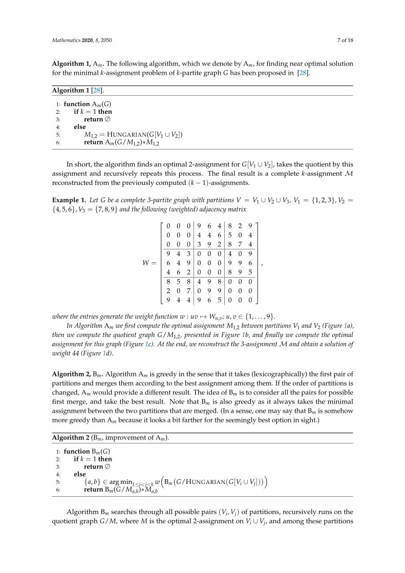
Algorithm 1, Am. The following algorithm, which we denote by Am, for finding near optimal solutionfor the minimal k-assignment problem of k-partite graph G has been proposed in [28].

Algorithm 1 [28].

1: function Am(G)2: if k = 1 then3: return ∅4: else5: M1,2 = HUNGARIAN(G[V1 ∪V2])6: return Am(G/M1,2)∗M1,2

In short, the algorithm finds an optimal 2-assignment for G[V1 ∪V2], takes the quotient by thisassignment and recursively repeats this process. The final result is a complete k-assignment Mreconstructed from the previously computed (k− 1)-assignments.

Example 1. Let G be a complete 3-partite graph with partitions V = V1 ∪ V2 ∪ V3, V1 = {1, 2, 3}, V2 =

{4, 5, 6}, V3 = {7, 8, 9} and the following (weighted) adjacency matrix

W =

0 0 0 9 6 4 8 2 90 0 0 4 4 6 5 0 40 0 0 3 9 2 8 7 49 4 3 0 0 0 4 0 96 4 9 0 0 0 9 9 64 6 2 0 0 0 8 9 58 5 8 4 9 8 0 0 02 0 7 0 9 9 0 0 09 4 4 9 6 5 0 0 0

,

where the entries generate the weight function w : uv 7→Wu,v; u, v ∈ {1, . . . , 9}.In Algorithm Am we first compute the optimal assignment M1,2 between partitions V1 and V2 (Figure 1a),

then we compute the quotient graph G/M1,2, presented in Figure 1b, and finally we compute the optimalassignment for this graph (Figure 1c). At the end, we reconstruct the 3-assignmentM and obtain a solution ofweight 44 (Figure 1d).

Algorithm 2, Bm. Algorithm Am is greedy in the sense that it takes (lexicographically) the first pair ofpartitions and merges them according to the best assignment among them. If the order of partitions ischanged, Am would provide a different result. The idea of Bm is to consider all the pairs for possiblefirst merge, and take the best result. Note that Bm is also greedy as it always takes the minimalassignment between the two partitions that are merged. (In a sense, one may say that Bm is somehowmore greedy than Am because it looks a bit farther for the seemingly best option in sight.)

Algorithm 2 (Bm, improvement of Am).

1: function Bm(G)2: if k = 1 then3: return ∅4: else5: {a, b} ∈ arg min1≤i<j<k w

(Bm(G/HUNGARIAN(G[Vi ∪Vj])

))6: return Bm(G/Ma,b)∗Ma,b

Algorithm Bm searches through all possible pairs (Vi, Vj) of partitions, recursively runs on thequotient graph G/M, where M is the optimal 2-assignment on Vi ∪ Vj, and among these partitions

Mathematics 2020, 8, 2050 8 of 18

chooses the one with the best assignment of G/M. If there are more minimal partitions, the algorithmchooses a random partition of minimal weight. Clearly, Algorithm Bm returns a k-assignment that isdetermined by the (k− 1) 2-assignments that were chosen in the recursive calls of Bm.

Example 2. We take the same graph as in Example 1. In contrast to Am, Algorithm Bm finds optimalassignments M1,2, M1,3, and M2,3 for the induced subgraphs G[V1 ∪ V2], G[V1 ∪ V3], and G[V2 ∪ V3],see Figure 2a–c, respectively. The algorithm continues its search recursively on the bipartite graphs G/M1,2,G/M1,3, and G/M2,3. As Figure 2b shows, we obtain a k-assignment of weight 40.

V1V2

V3

21

35

6

4 344

7 8 9

V1V2

V3

21

35

6

4 344

7 8 9

8 2649 4

(a) Solutionfrom M1,2

of weightw = 44.

V1V2

V3

21

35

6

4

2

7 8 9

5 4

V1V2

V3

21

35

6

4

2

7 8 9

5 4

294

50

9

(b) Solutionfrom M1,3

of weightw = 40.

V1V2

V3

21

35

6

4

7 8 9

860

V1V2

V3

21

35

6

4

7 8 9

860

8 0 9

4

62

(c) Solutionfrom M2,3

of weightw = 43.

Figure 2. Cases for Algorithm BM.

Algorithm 3, Cm. Observe that Algorithm Bm is much more time consuming than Algorithm Am as itcalls the Hungarian algorithm subroutine(

k2

)(k− 1

2

)· · ·(

32

)=

k!(k− 1)!2k−1

times as opposed to only (k− 1) calls by Algorithm Am.However, note that Algorithm Bm is greedy because it always takes the minimal 2-assignment.

As the k-assignment problem (for k > 2) is intractable, a deterministic greedy algorithm can notsolve the problem to optimality unless P=NP. We therefore consider an iterative improvement ofthe solutions by taking a nearly optimal solution (that may be the result of Bm) to define an initialsolution. The neighbors of the given solution are the results of the following procedure: fix one ofthe 2-assignments, say M, and run Algorithm Bm on G/M. After repeating the process by fixingall 2-assignments, we get a set of new solutions. If at least one of them is an improvement over thepreviously known best solution, we continue the improvement process. The process stops when thereis no better solution among the set of new solutions.

The third algorithm, denoted as Algorithm Cm, can be considered as a steepest descent algorithmon the set of all k-assignments, where the next solution is chosen to be a minimal solution in a suitablydefined neighborhood.

Mathematics 2020, 8, 2050 9 of 18

Algorithm 3 (Cm, steepest descent based on Bm).

1: function Cm(G)2: M =Bm(G)3: repeat4: Mprevious =M5: Ma,b = arg minMi,j∈M w

(Bm(G/Mi,j)

)6: M = Bm(G/Ma,b) ∗Ma,b7: until w(Mprevious) = w(M)8: returnM

Example 3. Taking the same instance as in Examples 1 and 2, Algorithm Cm starts with finding a 3-assignmentM = {M1,2, M1,3, M2,3} using Bm and continues by recursively searching graphs G/M1,2 and G/M2,3 (wecan skip G/M1,3, since the initial 3-assignment was already obtained from G/M1,3). As Figure 3 shows, the bestsolution of weight 37 is obtained from contracting M2,3. If we continue with the iteration, we can see that thesolution has stabilized and no further improvements can be made.

V1V2

V3

21

35

6

4

2

7 8 9

5 4

294

50

9

V1V2

V3

21

35

6

4

7 8 9

V1V2

V3

21

35

6

4

7 8 9

294

50

9

V1V2

V3

21

35

6

4

7 8 9

50

9

V1V2

V3

21

35

6

4

2

7 8 9

5 4

294

50

9

42

6

8

40

Figure 3. Cases for Algorithm Cm.

Algorithm 4, Dm. Algorithms Bm and Cm heavily rely on the Hungarian method and are verytime-consuming in comparison to Am. Therefore we define another greedy algorithm based on theHungarian method that is faster. We denote by Dm the greedy algorithm that takes the minimal2-assignment Mi,j in the k-partite graph G, and continues considering the (k− 1)-partite graph G/Mi,juntil only one partition is left.

Algorithm 4 (Dm, Greedy iterative)

1: function Dm(G)2: if k = 1 then3: return ∅4: else5: {a, b} ∈ arg min1≤i<j<k w

(HUNGARIAN(G[Vi ∪Vj])

)6: return Dm(G/Ma,b)∗Ma,b

Mathematics 2020, 8, 2050 10 of 18

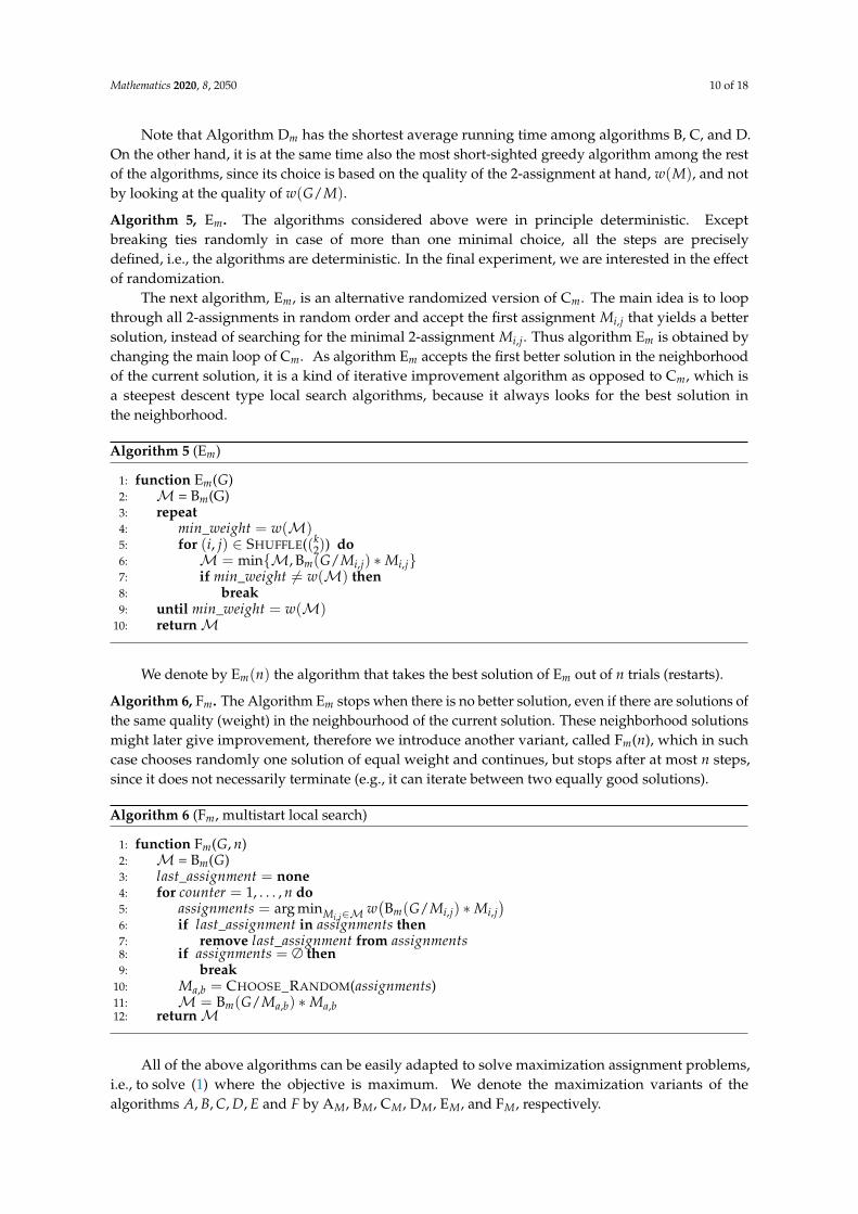
Note that Algorithm Dm has the shortest average running time among algorithms B, C, and D.On the other hand, it is at the same time also the most short-sighted greedy algorithm among the restof the algorithms, since its choice is based on the quality of the 2-assignment at hand, w(M), and notby looking at the quality of w(G/M).

Algorithm 5, Em. The algorithms considered above were in principle deterministic. Exceptbreaking ties randomly in case of more than one minimal choice, all the steps are preciselydefined, i.e., the algorithms are deterministic. In the final experiment, we are interested in the effectof randomization.

The next algorithm, Em, is an alternative randomized version of Cm. The main idea is to loopthrough all 2-assignments in random order and accept the first assignment Mi,j that yields a bettersolution, instead of searching for the minimal 2-assignment Mi,j. Thus algorithm Em is obtained bychanging the main loop of Cm. As algorithm Em accepts the first better solution in the neighborhoodof the current solution, it is a kind of iterative improvement algorithm as opposed to Cm, which isa steepest descent type local search algorithms, because it always looks for the best solution inthe neighborhood.

Algorithm 5 (Em)

1: function Em(G)2: M = Bm(G)3: repeat4: min_weight = w(M)5: for (i, j) ∈ SHUFFLE((k

2)) do6: M = min{M, Bm(G/Mi,j) ∗Mi,j}7: if min_weight 6= w(M) then8: break9: until min_weight = w(M)

10: returnM

We denote by Em(n) the algorithm that takes the best solution of Em out of n trials (restarts).

Algorithm 6, Fm. The Algorithm Em stops when there is no better solution, even if there are solutions ofthe same quality (weight) in the neighbourhood of the current solution. These neighborhood solutionsmight later give improvement, therefore we introduce another variant, called Fm(n), which in suchcase chooses randomly one solution of equal weight and continues, but stops after at most n steps,since it does not necessarily terminate (e.g., it can iterate between two equally good solutions).

Algorithm 6 (Fm, multistart local search)

1: function Fm(G, n)2: M = Bm(G)3: last_assignment = none4: for counter = 1, . . . , n do5: assignments = arg minMi,j∈M w

(Bm(G/Mi,j) ∗Mi,j

)6: if last_assignment in assignments then7: remove last_assignment from assignments8: if assignments = ∅ then9: break

10: Ma,b = CHOOSE_RANDOM(assignments)11: M = Bm(G/Ma,b) ∗Ma,b12: returnM

All of the above algorithms can be easily adapted to solve maximization assignment problems,i.e., to solve (1) where the objective is maximum. We denote the maximization variants of thealgorithms A, B, C, D, E and F by AM, BM, CM, DM, EM, and FM, respectively.

Mathematics 2020, 8, 2050 11 of 18

Remark 1. Clearly, the algorithms C, D, E, and F always return a feasible assignment because any solution isobtained by a recursive call of B. However, many calls of B and thus many runs of the Hungarian algorithmare expensive in terms of computation time. Therefore, it is an interesting question whether the present localsearch heuristics may be sped up by considering other neighborhoods, for example applying the idea of variableneighborhood search [29].

4. Numerical Results

In this section, we present numerical evaluations of the algorithms introduced in Section 3.We compare them with the algorithms from [28] and to each other. In particular, we

• reproduce the results on random graphs as given in [28] and compare them with the results ofour Algorithms Bm to Fm and their maximization variants BM to FM,

• evaluate the performance of the algorithms against AM as the number of vertices increases,• test our algorithms on the instances provided in [15].

4.1. Datasets

Numerical evaluations are done using three sets of random complete k-partite graphs. The first setwas constructed according to [28], as follows: It consists of two sets of 1000 random complete k-partitegraphs with k = 3, 4 and n = 30, 100, respectively. The weights on the edges were selected randomlyfrom given set S with probability density function p(x) = 1

|S| , ∀x ∈ S, where S = {0, 1, . . . , 9}, if k = 3and S = {1, . . . , 100}, if k = 4.

The second dataset is our contribution. It has been designed to compare how our algorithms scalewith increasing size of the instances. It consists of two subsets, each consisting of instances with k = 3and k = 4. The first subset was generated as follows. For each k ∈ {3, 4} we range the number ofvertices n in each partition from 2 to 100 and the weights on edges connecting vertices from differentpartitions are chosen randomly according to discrete uniform distribution on the set S = {0, . . . , n− 1}.The second subset was obtained similarly, we only changed the distribution of the edge weights.The edges between the different partitions are assigned random weights chosen according to discreteuniform distribution on the set S = {20, 21, . . . , 210}. We expect that these random instances are moredifficult, because the very important edges are sufficiently rare. For each pair k, n we generated 1000random instances.

The third set is the same as in [15]. For this set, the optimum value of 3-AP is known. We retrievedit from [30]. This dataset includes 18 instances of complete 3-partite graphs:

• 6 graphs with 33 vertices and 6 graphs with 66 vertices in each of the 3 partitions, where theweights of edges between different partitions are random integers which should, according to thedescription given by the authors [30], range from 0 to 99. However, we point out that some of theweights in these instances are larger than 100.

• 3 graphs with 33 vertices and 3 graphs with 66 vertices in each partition, where the weights takeonly values 1 or 2. We call these graphs binary graphs.

At the beginning of the web page [30] it is explained how the numerical results from [15] relate tothese instances.

4.2. First Experiment–Dataset from He et al. (2004)

In the first experiment we compare the algorithms used in [28] (namely, the Random,Greedy, and AM algorithm) with our Algorithms BM, CM, DM, EM, EM(10), and FM(100) on the firstset of random k-partite graphs, which we generated as described in [28], see Section 4.1. We run these5 algorithms on each group of 1000 graph instances and report the average values in Tables 1 and 2.

Mathematics 2020, 8, 2050 12 of 18

Table 1. Comparison of Random, Greedy and AM algorithms from [28] with BM to FM algorithmsfor the maximization version of 3-AP. Each row contains average values of solutions obtained bythese algorithms, computed over 1000 random instances of complete k-partite graphs with n vertices,which are generated as described in Section 4.1. We can see that Algorithms BM to FM returnsubstantially better results.

k = 3, n = 30, k = 4, n = 100,S = {0, . . . , 9} S = {1, . . . , 100}

Algorithm val ∆AM (%) Time val ∆AM (%) Time

Random 405 −45.9 - 41806 −23.5 -Greedy 736 −1.8 - 52801 −3.0 -

AM 749.2 0 1 54,421.7 0 1BM 753.8 0.6 3.0 54,634.1 0.4 14.4CM 759.4 1.4 6.1 54,731.5 0.6 46.7DM 749.4 0.0 2.4 54,442.9 0.0 3.7EM 759.3 1.3 5.3 54,730.5 0.6 37.9

EM(10) 759.9 1.4 53.0 54,761.1 0.6 378.7FM(100) 760.4 1.5 94.8 54,732.0 0.6 674.7

Table 2. The rows contain (respectively) the average values obtained by algorithms Random,Greedy, Am from [28], and by our Algorithms Bm to Cm over 1000 random complete 3-partite graphs,respectively. We can see that our Algorithms Bm to Fm outperform the algorithms from [28].

k = 3, n = 30,S = {0, . . . , 9}

Algorithm val ∆Am(%) Time

Random 405 566.7 -Greedy 218 258.9 -

Am 60.7 0 1Bm 56.2 −7.4 3Cm 50.8 −16.4 6.1Dm 60.6 −0.2 2.4Em 50.9 −16.2 5.3

Em(10) 50.3 −17.2 53Fm(100) 49.8 −18.0 95.2

In order to compare the algorithms with Am (resp. AM), we define the relative gap with respect tothe value obtained by Am (resp. AM) by

∆Am = 100 · val− valAm

valAm

(resp. ∆AM = 100 ·

val− valAM

valAM

).

4.3. Second Experiment on Random Instances

In this subsection we compare Algorithms BM, CM, DM, EM, EM(10), and FM(100) on the seconddataset, introduced in Section 4.1. We run all three algorithms on each of two subsets, consisting of1000 instances for each pair (k, n) ∈ {3, 4} × {2, 3, 4, . . . , 100}. For each pair (k, n) and each algorithm,we compute the average value of solutions given by the algorithm over the corresponding 1000instances. Then, we compute quotients of the average values for BM and for AM and denote itby BM/AM. Similarly we compute quotient CM/AM, and so on. Figures 4–7 contain plots andinterpretations of these quotients.

The results on the first subset (with uniform distribution of weights) are depicted onFigures 4 and 5. They show that Algorithm EM(10) clearly finds the best solutions. The AlgorithmsCM, EM and FM(100) perform similarly, and are clearly outperforming BM and DM. Note that takinginto account time complexity and considering k = 3, the clear winners among the faster algorithms(AM, BM, CM, DM, and EM) are CM and EM, and among the more time consuming EM(10) and FM(100),

Mathematics 2020, 8, 2050 13 of 18

the winner is EM(10). Note that EM(n) may potentially find even better solutions with larger n (andconsequently may need more time). The differences are much less obvious for k = 4 (see Figure 5).With larger n, the ratios seem to stabilize at certain constants.

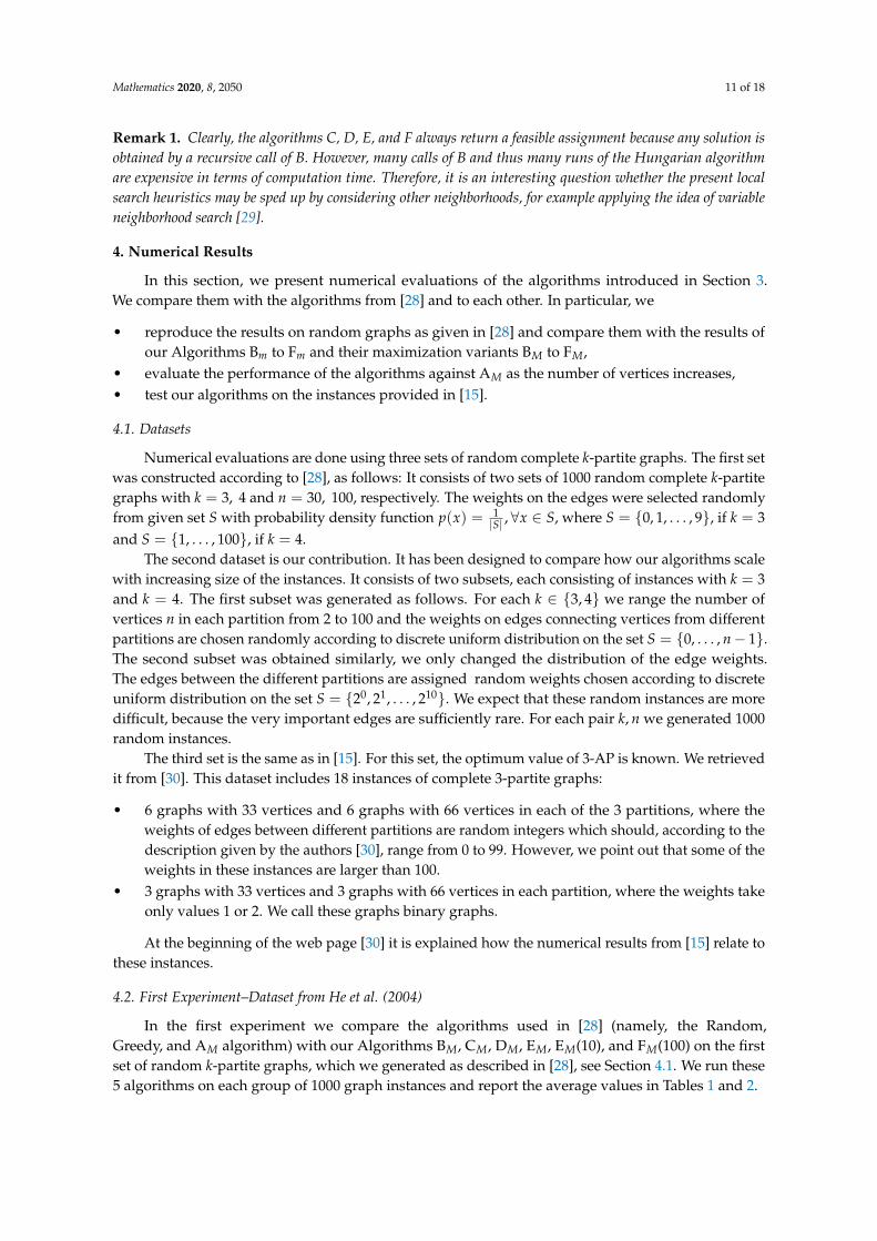
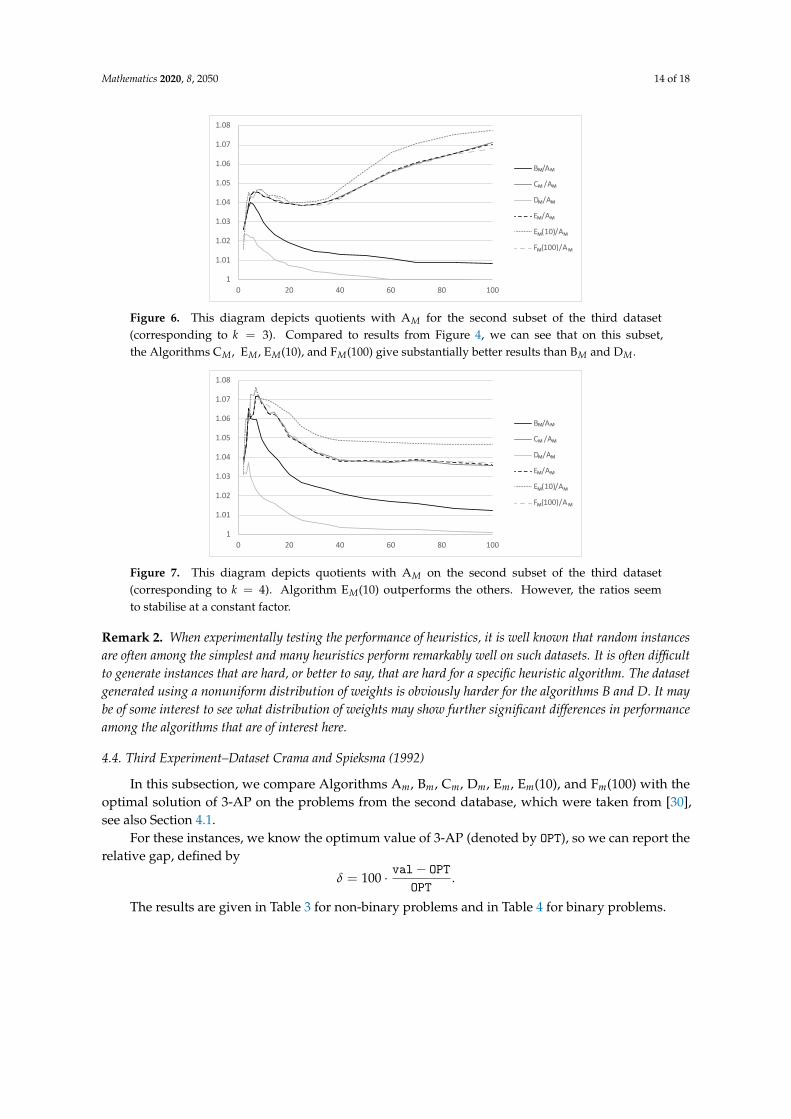
Considering the results on the first dataset (Table 1) and the first sample of the second dataset(Figures 4 and 5) suggest that there is no significant difference in quality of solutions among thealgorithms C, E, and F. However, the results on the second subset (the set with a special distributionof weights), in particular for k = 3, show that Algorithms C, E, and F substantially outperform B andD (see Figure 6), and the differences of ratios tend to grow with larger n. This allows us to concludethat Algorithms CM, EM(n) and FM(n) are significantly better than BM and DM (at least on most of ourinstances). For k = 4 (see Figure 7), the differences are small again.

1

1.01

1.02

1.03

1.04

0 20 40 60 80 100

B /A

C /A

D /A

E /A

E (10)/A

F (100)/A

M M

M M

M M

M M

M M

M M

Figure 4. This plot depicts the quotients with AM for the instances from the first subset of the thirddataset (see Section 4.1) corresponding to k = 3. The x axis represents the size of each partition n,while the y axis represents the quotient. We can see that with larger n, EM(10) outperforms all otheralgorithms, while CM, EM, and FM(100) perform similarly.

1

1.01

1.02

1.03

1.04

0 20 40 60 80 100

B /A

C /A

D /A

E /A

E (10)/A

F (100)/A

M M

M M

M M

M M

M M

M M

Figure 5. On this plot we can observe the quotients with AM for the instances from the first subset ofthe third dataset, corresponding to k = 4. The x axis represents the size of each partition n, while yaxis represents the quotient. Compared to results from Figure 4, we can see that on this dataset,the difference between BM, CM, EM, EM(10) and FM(100) are becoming almost negligible whenn increases.

Mathematics 2020, 8, 2050 14 of 18

1

1.01

1.02

1.03

1.04

1.05

1.06

1.07

1.08

0 20 40 60 80 100

B /A

C /A

D /A

E /A

E (10)/A

F (100)/A

M M

M M

M M

M M

M M

M M

Figure 6. This diagram depicts quotients with AM for the second subset of the third dataset(corresponding to k = 3). Compared to results from Figure 4, we can see that on this subset,the Algorithms CM, EM, EM(10), and FM(100) give substantially better results than BM and DM.

1

1.01

1.02

1.03

1.04

1.05

1.06

1.07

1.08

0 20 40 60 80 100

B /A

C /A

D /A

E /A

E (10)/A

F (100)/A

M M

M M

M M

M M

M M

M M

Figure 7. This diagram depicts quotients with AM on the second subset of the third dataset(corresponding to k = 4). Algorithm EM(10) outperforms the others. However, the ratios seemto stabilise at a constant factor.

Remark 2. When experimentally testing the performance of heuristics, it is well known that random instancesare often among the simplest and many heuristics perform remarkably well on such datasets. It is often difficultto generate instances that are hard, or better to say, that are hard for a specific heuristic algorithm. The datasetgenerated using a nonuniform distribution of weights is obviously harder for the algorithms B and D. It maybe of some interest to see what distribution of weights may show further significant differences in performanceamong the algorithms that are of interest here.

4.4. Third Experiment–Dataset Crama and Spieksma (1992)

In this subsection, we compare Algorithms Am, Bm, Cm, Dm, Em, Em(10), and Fm(100) with theoptimal solution of 3-AP on the problems from the second database, which were taken from [30],see also Section 4.1.

For these instances, we know the optimum value of 3-AP (denoted by OPT), so we can report therelative gap, defined by

δ = 100 · val− OPT

OPT.

The results are given in Table 3 for non-binary problems and in Table 4 for binary problems.

Mathematics 2020, 8, 2050 15 of 18

Table 3. Comparison of Algorithms Am, Bm, Cm, Dm, Em, Em(10), and Fm(100) on the first group ofinstances of 3-AP from [15,30]. Column 2 contains the optimum value of the problem, as reportedin [30]. For each algorithm, we report the value that it returns. Average relative errors δ and averagecomputation times are given in the last two rows. Algorithms Cm, Em, Em(10), and Fm(100) have thebest performance and, on average, differ from the optimal solution by 0.1% or less (see the last row).

Problem OPT Am Bm Cm Dm Em Em(10) Fm(100)

3DA198N1 2662 2696 2669 2663 2669 2663 2663 26633DA198N2 2449 2498 2467 2458 2467 2458.4 2457.1 2457.43DA198N3 2758 2811 2778 2764 2778 2764 2764 27643DA99N1 1608 1617 1617 1608 1617 1608.0 1608.0 1608.03DA99N2 1401 1420 1411 1402 1415 1402.0 1402.0 1402.03DA99N3 1604 1612 1612 1604 1612 1604.0 1604.0 1604.03DI198N1 9684 9830 9765 9695 9765 9693.3 9689.2 9689.83DI198N1 8944 9132 9121 8949 9177 8949.7 8947.4 8948.43DI198N3 9745 9930 9876 9750 9876 9749.6 9747.6 9748.53DIJ99N1 4797 4882 4839 4800 4882 4801.3 4798 4799.33DIJ99N2 5067 5145 5136 5074 5145 5071.8 5069.6 5071.13DIJ99N3 4287 4338 4338 4291 4371 4290.5 4287.8 4289.6

δ[%] 0 1.47 0.92 0.10 1.15 0.10 0.07 0.08Time - 1 2.9 11.8 2.3 9.0 89.1 150.9

Table 4. Numerical result for Algorithms Am, Bm, and Cm on the second group of instances from [30](called binary graphs). The optimum values OPT are taken from [30], and the values val are computedby Algorithms Am, Bm, Cm, Dm, Em, Em(10), and F(100). Average relative errors δ and averagecomputation times are given in the last two rows. We can see that Fm(100) has the best performance.

Problem OPT Am Bm Cm Dm Em E(10) Fm(100)

3Dm198N1 286 298 294 287 295 286.5 286.0 286.43Dm198N2 286 294 293 286 294 286.2 286.0 286.23Dm198N3 282 294 294 285 294 284.9 284.3 283.73Dm299N1 133 140 134 134 134 134.0 134.0 133.43Dm299N2 131 139 137 134 137 134.0 134.0 133.03Dm299N3 131 136 136 132 136 132.0 132.0 131.0

δ[%] 0 4.41 3.11 0.87 3.22 0.84 0.77 0.45Time 0 1 2.7 6.8 2.4 5.4 54.0 89.7

For non-binary graphs, with results presented in Table 3, Algorithms Cm, Em, Em(10), and F(100)have, as expected, the best performance and on average differ from the optimal solution by 0.1% orless (see last row in Table 3). In addition, they are in some cases also able to find the optimal solution.

For binary graphs, with results presented in Table 4, we can observe that the relative performancesare, due to the low weight sum, worse than those of non-binary graphs. As the problems are binary,a solution that differs from the optimal in one element may have, due to small total weight of theassignments, a considerably large relative error. As in the case of non-binary graphs, Cm, Em, Em(10),and F(100) outperform Am, Bm, and Dm. Algorithm Fm(100) finds the optimal solution in most cases(see the last column), and Algorithms Cm, and Em find the optimal solution in some cases.

We point out that these algorithms are fast. Our implementation, which could be further optimised,takes a fraction of a second (on a 3.0 Ghz PC) on each of these instances. Relative computation times(relative to algorithm A) and average relative errors (compared to known optimal solutions) are evidentfrom Figure 8.

Mathematics 2020, 8, 2050 16 of 18

Figure 8. This diagram contains graphical representations of average (normalized) times (in logarithmicscale) needed for non-binary instances from [30] computed in Table 3 and relative errors rel(withrespect to the optimal value OPT). Algorithms Am, Bm, Cm, Dm, and Em are considered fast, while Em(10)and Fm(100) are comparably slow.

5. Summary and Conclusions

We have introduced Algorithms A, B, C, D, E, and F to approximately solve (1). The algorithmsare all based on extensive use of the Hungarian algorithm and thus arise as natural improvements ofAlgorithm A from [28]. Algorithms A, B, C, and D are in principle deterministic, whereas AlgorithmsE and F incorporate randomization. We implemented the algorithms in Python and evaluated them onthree benchmark datasets. Numerical tests show that new algorithms in minimization or maximizationvariant, in terms of solution quality, outperform A on all of the chosen datasets. Summing up, our studyshows that multiple usage of the classic Hungarian method can provide very tight solutions for (1),in some cases even an optimal solution.

Another important issue when regarding algorithms’ performance is computational time.For smaller instances, E has relatively good speed and on average misses the optimal solution by merely0.1%, thus, we propose it as our method of choice. Among the deterministic algorithms, our studysuggests using Algorithm C. However, we wish to note that when we consider large instances of (1),both in number of partitions and in size of each partition, we must be very careful how often we willactually run the Hungarian method because many repetitions of the Hungarian method substantiallyincrease computation time. The main goal of the reported research was to explore the potential ofthe Hungarian algorithm for solving the k-assignment problem. We have designed several heuristicsbased on the Hungarian method that have shown to be competitive. While, on one hand, some ofour algorithms provide very good (near optimal or even optimal) results in a short time, we alsodesigned two heuristics based on local search [31–33]. Local search type heuristics improve the qualityof solutions over time and may converge to the optimal solution. This type of heuristics are very usefulwhen the quality of solutions is more important than computational time. We believe that furtherdevelopment of a multistart local search heuristics based on the Hungarian algorithm may lead toa very competitive heuristics for (1) with hopefully competitive fast convergence to optimal solutions.

In the future, a more comprehensive experimental study of local search based on the Hungarianalgorithm may be a very promising avenue of research.

Author Contributions: Funding acquisition, J.P.; Methodology, J.Ž.; Software, B.G.; Supervision, J.P. and J.Ž.;Writing—original draft, B.G., T.N. and D.R.P.; Writing—review & editing, J.P. and J.Ž. All authors have read andagreed to the published version of the manuscript.

Funding: This reasearch is funded in part by Javna Agencija za Raziskovalno Dejavnost RS, grants: J1-8155,J1-1693, P2-0248, and J2-2512.

Mathematics 2020, 8, 2050 17 of 18

Acknowledgments: The authors wish to thank to three anonymous reviewers for a number of constructivecomments that helped us to considerably improve the presentation.

Conflicts of Interest: The authors declear have no conflicts of interest.

References

1. Gligorijevic, V.; Malod-Dognin, N.; Pržulj, N. Integrative methods for analyzing big data in precisionmedicine. Proteomics 2016, 16, 741–758.

2. Gligorijevic, V.; Malod-Dognin, N.; Pržulj, N. Fuse: Multiple network alignment via data fusion.Bioinformatics 2015, 32, 1195–1203, doi:10.1093/bioinformatics/btv731.

3. Malod-Dognin, N.; Petschnigg, J.; Windels, S.F.L.; Povh, J.; Hemmingway, H.; Ketteler, R.; Pržulj, N.Towards a data-integrated cell. Nat. Commun. 2019, 10, 805, doi:10.1038/s41467-019-08797-8.

4. Balas, E.; Saltzman, M.J. An algorithm for the three-index assignment problem. Oper. Res. 1991, 39, 150–161.5. Burkard, R.; Dell’Amico, M.; Martello, S. Assignment Problems: Revised Reprint; SIAM-Society of Industrial

and Applied Mathematics: Philadelphia, PA, USA, 2012; Volume 106, doi:10.1137/1.9781611972238.6. Burkard, R.E.; Rudolf, R.; Woeginger, G.J. Three-dimensional axial assignment problems with decomposable

cost coefficients. Discret. Appl. Math. 1996, 65, 123–139, doi:10.1016/0166-218X(95)00031-L.7. Frieze, A.M. Complexity of a 3-dimensional assignment problem. Eur. J. Oper. Res. 1983, 13, 161–164.8. Spieksma, F. Multi Index Assignment Problems: Complexity, Approximation, Applications. In Nonlinear

Assignment Problems; Springer: Boston, MA, USA, 2000; pp. 1–12, doi:10.1007/978-1-4757-3155-2_1.9. Kuroki, Y.; Matsui, T. An approximation algorithm for multidimensional assignment problems minimizing

the sum of squared errors. Discret. Appl. Math. 2009, 157, 2124–2135.10. Grundel, D.A.; Krokhmal, P.A.; Oliveira, C.A.S.; Pardalos, P.M. On the number of local minima for the

multidimensional assignment problem. J. Comb. Optim. 2007, 13, 1–18.11. Kuhn, H.W. The Hungarian Method for the Assignment Problem. Nav. Res. Logist. Q. 1955, 2, 83–97,

doi:10.1002/nav.3800020109.12. Karp, R.M. Reducibility Among Combinatorial Problems. In Complexity of Computer Computations;

Plenum: New York, NY, USA, 1972; pp. 85–103, doi:10.1007/978-1-4684-2001-2_9.13. Hurkens, C.A.J.; Schrijver, A. On the size of systems of sets every t of which have an SDR, with an application

to the worst-case ratio of heuristics for packing problems. SIAM J. Discret. Math. 1989, 2, 68–72.14. Arkin, E.; Hassin, R. On local search for weighted packing problems. Math. Oper. Res. 1998, 23, 640–648.15. Crama, Y.; Spieksma, F. Approximation algorithms for three-dimensional assignment problems with triangle

inequalities. Eur. J. Oper. Res. 1992, 60, 273–279, doi:10.1016/0377-2217(92)90078-N.16. Aiex, R.M.; Resende, M.G.C.; Paradalos, P.M.; Toraldo, G. Grasp with path relinking for three-index

assignment. Inform. J. Comput. 2005, 17, 224–247.17. Huang, G.; Lim, A. A hybrid genetic algorithm for the Three-Index Assignment Problem. Eur. J. Oper. Res.

2006, 172, 249–257.18. Gutin, G.; Karapetyan, D. Local Search Heuristics for the Multidimensional Assignment Problem. J. Heuristics

2011, 17, 201–249, doi:10.1007/s10732-010-9133-3n.19. Karapetyan, D.; Gutin, G.; Goldengorin, B. Empirical evaluation of construction heuristics for the

multidimensional assignment problem. arXiv 2009, arXiv:0906.2960.20. Jiang, H.; Zhang, S.; Ren, Z.; Lai, X.; Piao, Y. Approximate Muscle Guided Beam Search for

Three-Index Assignment Problem. Adv. Swarm Intell. Lect. Notes Comput. Sci. 2014, 8794, 44–52,doi:10.1007/978-3-319-11857-4-6.

21. Karapetyan, D.; Gutin, G. A New Approach to Population Sizing for Memetic Algorithms: A Case Study forthe Multidimensional Assignment Problem. Evol. Comput. 2011, 19, 345–371.

22. Valencia, C.E.; Zaragoza Martinez, F.J.; Perez, S.L.P. A simple but effective memetic algorithm for themultidimensional assignment problem. In Proceedings of the 14th Inernational Conference on ElectricalEngineering, Computing Science and Automatic Control (CCE), Mexico City, Mexico, 20–22 Octoner 2017;pp. 1 – 6, doi:10.1109/ICEEE.2017.8108889.

23. Li, J.; Tharmarasa, R.; Brown, D.; Kirubarajan, T.; Pattipati, K.R. A novel convex dual approach tothree-dimensional assignment problem: Theoretical analysis. Comput. Optim. Appl. 2019, 74, 481–516,doi:10.1007/s10589-019-00113-w.

Mathematics 2020, 8, 2050 18 of 18

24. O’Leary, B. Don’t be Greedy, be Neighborly, a new assignment algorithm. In Proceedings of the 2019 IEEEAerospace Conference, Big Sky, MT, USA, 2–9 March 2019; pp. 1–8.

25. Medvedev, S.N.; Medvedeva, O.A. An Adaptive Algorithm for Solving the Axial Three-Index AssignmentProblem. Autom. Remote Control 2019, 80, 718–732, doi:10.1134/S000511791904009X.

26. Pentico, D. Assignment problems: A golden anniversary survey. Eur. J. Oper. Res. 2007, 176, 774–793.27. Walteros, J.; Vogiatzis, C.; Pasiliao, E.; Pardalos, P. Integer programming models for the multidimensional

assignment problem with star costs. Eur. J. Oper. Res. 2014, 235, 553–568.28. He, G.; Liu, J.; Zhao, C. Approximation algorithms for some graph partitioning problems. In Graph Algorithms

and Applications 2; World Scientific: Singapore, 2004; pp. 21–31.29. Mladenovic, N.; Hansen, P. Variable neighborhood search. Comput. Oper. Res. 1997, 24, 1097–1100,

doi:10.1016/S0305-0548(97)00031-2.30. Spieksma, F.C.R. Instances of the 3-Dimensional Assignment Problem. Available online: https://www.win.

tue.nl/~fspieksma/instancesEJOR.htm (accessed on 15 February 2019).31. Aarts, E.H.L.; Lenstra, J.K. (Eds.) Local Search in Combinatorial Optimization; Wiley-Interscience Series in

Discrete Mathematics and Optimization; Wiley-Interscience: Hoboken, NJ, USA, 1997.32. Talbi, E. Metaheuristics: From Design to Implementation; John Wiley & Sons: Hoboken, NJ, USA, 2009.33. Žerovnik, J. Heuristics for NP-hard optimization problems—Simpler is better !? Logist. Sustain. Transp. 2015,

6, 1–10, doi:10.1515/jlst-2015-0006.

Publisher’s Note: MDPI stays neutral with regard to jurisdictional claims in published maps and institutionalaffiliations.

© 2020 by the authors. Licensee MDPI, Basel, Switzerland. This article is an open accessarticle distributed under the terms and conditions of the Creative Commons Attribution(CC BY) license (http://creativecommons.org/licenses/by/4.0/).