Multiple decisions about one object involve parallel sensory ...

*For correspondence:

[email protected] (YHRK);

[email protected] (MNS)

†These authors contributed

equally to this work‡These authors also contributed

equally to this work

Present address: §Department

of Engineering, University of

Cambridge, Cambridge, United

Kingdom

Competing interests: The

authors declare that no

competing interests exist.

Funding: See page 37

Received: 04 October 2020

Accepted: 06 March 2021

Published: 10 March 2021

Reviewing editor: Kristine Krug,

University of Oxford, United

Kingdom

Copyright Kang et al. This

article is distributed under the

terms of the Creative Commons

Attribution License, which

permits unrestricted use and

redistribution provided that the

original author and source are

credited.

Multiple decisions about one objectinvolve parallel sensory acquisition buttime-multiplexed evidence incorporationYul HR Kang1,2†§*, Anne Loffler1,3†, Danique Jeurissen1,4†, Ariel Zylberberg1,5‡,Daniel M Wolpert1‡, Michael N Shadlen1,3,4‡*

1Zuckerman Mind Brain Behavior Institute, Department of Neuroscience, ColumbiaUniversity, New York, United States; 2Department of Engineering, University ofCambridge, Cambridge, United Kingdom; 3Kavli Institute for Brain Science,Columbia University, New York, United States; 4Howard Hughes Medical Institute,Columbia University, New York, United States; 5Department of Brain and CognitiveSciences, University of Rochester, Rochester, United States

Abstract The brain is capable of processing several streams of information that bear on

different aspects of the same problem. Here, we address the problem of making two decisions

about one object, by studying difficult perceptual decisions about the color and motion of a

dynamic random dot display. We find that the accuracy of one decision is unaffected by the

difficulty of the other decision. However, the response times reveal that the two decisions do not

form simultaneously. We show that both stimulus dimensions are acquired in parallel for the initial

~0.1 s but are then incorporated serially in time-multiplexed bouts. Thus, there is a bottleneck that

precludes updating more than one decision at a time, and a buffer that stores samples of evidence

while access to the decision is blocked. We suggest that this bottleneck is responsible for the long

timescales of many cognitive operations framed as decisions.

IntroductionDecisions are often informed by several aspects of a problem, each guided by different sources of

information. In many instances, these aspects are combined to support a single judgment. For exam-

ple, an observer might judge the distance of an animal by combining perspective cues, binocular dis-

parity and motion parallax. In other instances, the aspects are distinct dimensions of the same

object. For example, the animal’s distance and its identity as potential predator or prey. The former

problem of cue combination (Jacobs, 1999; Ernst and Banks, 2002) is a topic of study in what has

been termed the Bayesian Brain (Knill and Pouget, 2004). The latter is the subject of this paper. It

arises in a wide variety of problems whose solutions depend on identifying a set of conjunctions

such as the ingredients of a favorite dish, or when one must make multiple judgments, or decisions,

about the same stimulus.

The neuroscience of decision-making has focused largely on perceptual decisions, contrived to

promote the integration of noisy evidence over time toward a categorical choice about one stimulus

dimension. A well-studied example is a decision about the net direction of motion of randomly mov-

ing dots. In such binary decisions (e.g. left or right), behavioral and neural studies have shown that

humans and monkeys accumulate noisy samples of evidence and commit to a choice when the accu-

mulated evidence reaches a threshold (Ratcliff, 1978; Palmer et al., 2005; Gold and Shadlen,

2007; Stine et al., 2020). The framework has been extended to more than two categories (e.g.

Churchland et al., 2008; Bogacz et al., 2007; Ditterich, 2010) but it remains focused on a common

stream of evidence bearing on a single stimulus feature. Less is known about how multiple streams

Kang, Loffler, Jeurissen, et al. eLife 2021;10:e63721. DOI: https://doi.org/10.7554/eLife.63721 1 of 44

RESEARCH ARTICLE

http://creativecommons.org/licenses/by/4.0/

http://creativecommons.org/licenses/by/4.0/

https://doi.org/10.7554/eLife.63721

https://creativecommons.org/

https://creativecommons.org/

https://elifesciences.org/?utm_source=pdf&utm_medium=article-pdf&utm_campaign=PDF_tracking

https://elifesciences.org/?utm_source=pdf&utm_medium=article-pdf&utm_campaign=PDF_tracking

http://en.wikipedia.org/wiki/Open_access

http://en.wikipedia.org/wiki/Open_access

of evidence are accumulated for a multidimensional decision (Lorteije et al., 2015). Given the paral-

lel organization of the sensory systems, one might expect all available evidence to be integrated

simultaneously. However, there are also reasons to suspect that two decisions cannot be made in

parallel. This is based on a variety of experiments that expose a ‘psychological refractory period’

(PRP; Welford, 1952). When participants are asked to make two decisions in a rapid succession, it

appears that the second decision is delayed until the first decision is complete (Pashler, 1994).

Based on such observations, it has been argued that there is a structural bottleneck in the response

selection step, such that only one response can be selected at a time (Sigman and Dehaene, 2005).

Here, we develop a task in which the participant views one visual stimulus and makes two deci-

sions about the same object. The stimulus comprises elements that give rise to two streams of evi-

dence bearing on their motion and color, and the participant must decide on both aspects and

report the combined category. The task was designed to allow participants to integrate both

streams of evidence simultaneously from the same location in the visual field and to indicate both

choices with just one response. We show that, even in this situation, the two streams of evidence are

accumulated one at a time, and moreover, this seriality arises despite the parallel access of the visual

system to both streams. We suggest that seriality is explained by a bottleneck between the parallel

acquisition of evidence and its incorporation into separate decision processes. We elaborate a

model of bounded evidence accumulation, used previously to explain both the speed and accuracy

of motion (Palmer et al., 2005) and color decisions (Bakkour et al., 2019), and show that these

accumulations must occur in series. The results have implications for a variety of psychological obser-

vations concerning sequential vs. parallel operations, and they address the fundamental question of

why mental processes take the time they do.

ResultsWe studied variants of a perceptual task that required binary decisions about two properties of a

dynamic random dot display. Human participants decided the dominant color and direction of motion

in a small patch of dynamic random dots (Figure 1). The stimulus is similar to one introduced by

Mante et al., 2013, who studied the problem of gating when making a decision about only a single

dimension, either color or motion. On each video frame, each dot has a probability of being colored

blue or yellow and it has another probability of being plotted either at a displacement Dx relative to a

dot shown 40 ms earlier or, alternatively, at a random location in the display. We refer to the probabil-

ity of a displacement as the coherence or strength and use its sign to designate the direction. We use

an analogous signed probability for the color coherence or strength (see Materials and methods). In

the main tasks, participants reported their answer by making an eye or hand movement to select one

of four choice targets. We refer to this as a double-decision and refer to the two aspects as stimulus

dimensions. We employed several variants of this basic task in our study.

Roadmap of the experimental resultsWe first present the main finding using a free response paradigm, what we term double-decision

reaction time (Experiment 1). It demonstrates no interference in choice accuracy—that is, the diffi-

culty of the color decision does not affect the accuracy of motion decisions, and vice versa—but criti-

cally, the double-decision (2D) time is the sum of the two single-decision (1D) times. The analysis

suggests that the motion and color decisions are not formed at the same time. This establishes the

prediction that with brief stimulus presentations, successful color decisions ought to be attained at

the expense of motion, and vice versa—that is, choice interference. We then test this prediction

(Experiment 2) and fail to confirm it. We show that color and motion can be acquired in parallel but

are unable to update the decision simultaneously. This confirms the response selection bottleneck

predicted by Pashler (Fagot and Pashler, 1992) and it implies the existence of buffers (Sperl-

ing, 1960; Kamienkowski and Sigman, 2008), where sensory information can be held before it

updates a decision variable—the accumulated evidence for color or motion.

The combination of a buffer and serial updating leads to a revised prediction that interference in

accuracy should occur over a narrow range of stimulus viewing duration, controlled by the experi-

menter. We confirm this prediction (Experiment 3), showing that there is no interference at short

viewing times, but that there is a narrow regime of the stimulus duration in which accuracy on one

dimension suffers because a limited amount of deliberation time needs to be shared with the other


Research article Neuroscience


dimension, which reconciles conflicting observations of parallel and serial patterns of decision-mak-

ing in the literature (e.g. Schumacher et al., 2001; Tombu and Jolicoeur, 2004). We then introduce

a bimanual version of the task (Experiment 4) which affords direct reports of both the color and

motion termination times. It confirms the assumption that the double-decision time is the sum of

two sequential sampling processes, each with its own stopping time, and it shows that the color and

motion decisions compete before the first decision terminates. This implies some form of time-multi-

plexed alternation. In the last experiment, we ask participants to judge whether the motion in a pair

of patches is the same or different (Experiment 5) and find that this binary decision, based only on

motion processing, also exhibits additive decision times. Finally, we introduce a conceptual model of

the double-decision process that serves as a platform to connect the computational elements with

known and unknown neural mechanisms.

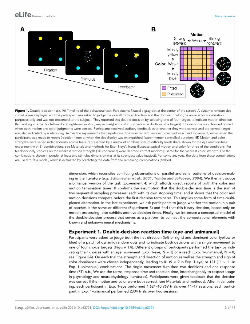
Experiment 1. Double-decision reaction time (eye and unimanual)Participants were asked to judge both the net direction (left or right) and dominant color (yellow or

blue) of a patch of dynamic random dots and to indicate both decisions with a single movement to

one of four choice targets (Figure 1A). Different groups of participants performed the task by indi-

cating their choices with an eye movement (Exp. 1-eye, N = 3) or a reach (Exp. 1-unimanual, N = 8;

see Figure 5A). On each trial the strength and direction of motion as well as the strength and sign of

color dominance were chosen independently, leading to 81 (9 � 9 in Exp. 1-eye) or 121 (11 � 11 in

Exp. 1-unimanual) combinations. The single movement furnished two decisions and one response

time (RT; n.b., We use the terms, response time and reaction time, interchangeably to respect usage

in psychology and neurophysiology literatures). Participants were given feedback that the decision

was correct if the motion and color were both correct (see Materials and methods). After initial train-

ing, each participant in Exp. 1-eye performed 4,624–10,969 trials over 11–17 sessions; each partici-

pant in Exp. 1-unimanual performed 2304 trials over two sessions.

Figure 1. Double decision task. (A) Timeline of the behavioral task. Participants fixated a gray dot at the center of the screen. A dynamic random dot

stimulus was displayed and the participant was asked to judge the overall motion direction and the dominant color (the arrow is for visualization

purposes only and was not presented to the subject). They reported this double-decision by selecting one of four targets to indicate motion direction

(left and right target for leftward and rightward motion, respectively) and color (top yellow vs. bottom blue targets). The response was deemed correct

when both motion and color judgments were correct. Participants received auditory feedback as to whether they were correct and the correct target

was also indicated by a white ring. Across the experiments the targets could be selected with an eye movement or a hand movement, either when the

participant was ready to report (reaction time) or when the dot display was extinguished (experimenter-controlled duration). (B) Motion and color

strengths were varied independently across trials, represented by a matrix of combinations of difficulty levels (here shown for the eye reaction-time

experiment with 81 combinations; see Materials and methods for Exp. 1-eye). Insets illustrate typical motion and color for three of the conditions. For

feedback only, choices on the weakest motion strength (0% coherence) were deemed correct randomly; same for the weakest color strength. For the

combinations shown in purple, at least one stimulus dimension was at its strongest value (easiest). For some analyses, the data from these combinations

are used to fit a model, which is evaluated by predicting the data from the remaining combinations (amber).




Figure 2A,B shows choices and mean RT as a function of stimulus strength for the eye and unima-

nual tasks, respectively. The graphs in the left column of each panel show the data plotted as a func-

tion of motion strength and direction. Each color on this graph corresponds to a different difficulty

-1 -0.5 0 0.5 1

Motion strength (norm.)

0

0.2

0.4

0.6

0.8

1

Pro

po

rtio

n r

igh

twa

rd c

ho

ice

s

low

high

-1 -0.5 0 0.5 1

Color strength (norm.)

0

0.2

0.4

0.6

0.8

1

Pro

po

rtio

n b

lue

ch

oic

es

low

high

Motion strength

0.5

1

1.5

2

Re

sp

on

se

tim

e (

s)

0.5

1

1.5

2

-1 -0.5 0 0.5 1

Motion strength (norm.)

0.5

1

1.5

2

Re

sp

on

se

tim

e (

s)

-1 -0.5 0 0.5 1

Color strength (norm.)

0.5

1

1.5

2

-0.5 0 0.5

Motion strength (coh.)

0

0.2

0.4

0.6

0.8

1

Pro

po

rtio

n r

igh

twa

rd c

ho

ice

s

-0.5 0 0.5

Color strength (coh.)

0

0.2

0.4

0.6

0.8

1

Pro

po

rtio

n b

lue

ch

oic

es

Motion strength

0.5

1

1.5

2

2.5

Re

sp

on

se

tim

e (

s)

0.5

1

1.5

2

2.5

-0.5 0 0.5


0.5

1

1.5

2

2.5

Re

sp

on

se

tim

e (

s)

-0.5 0 0.5


0.5

1

1.5

2

2.5

A BEye Unimanual

fit predictColor strength

fit predictlow

high

predictColor strength

fit

high

predictfitlow

Figure 2. Double-decisions exhibit additive response times but no interference in accuracy (Experiment 1). Participants judged the dominant color and

direction of dynamic random dots and indicated the double-decision by an eye movement (A; Exp. 1-eye) or reach (B; Exp. 1-unimanual) to one of four

choice-targets. All graphs show the behavioral measure (proportion of choices, top row; mean RT, rows 2 and 3) as a function of either signed motion

or color strength. Positive and negative color strength indicate blue- or yellow-dominance, respectively. Positive and negative motion strength indicate

rightward or leftward, respectively. Colors of symbols and traces indicate the difficulty (unsigned coherence) of the other stimulus dimension (e.g.,

color, for the graphs with abscissae labeled ’Motion strength’). Symbols are combined data from three participants (Exp. 1-eye) and eight participants

(Exp. 1-unimanual). Open symbols identify the conditions used to fit the serial (middle row) and parallel (bottom row) models. These are the conditions

in which at least one of the two stimulus strengths was at its maximum (purple shading, Figure 1B). In the top row, fits of the serial and parallel models

are shown by solid and dashed lines, respectively. The models comprise two bounded drift-diffusion processes, which explain the choices and decision

times as a function of either color or motion. They differ only in the way they combine the decision times to explain the double-decision RT. For the

serial model, the double-decision time is the sum of the color and motion decision times. For the parallel model, the double-decision time is the longer

of the color and motion decisions (see Materials and methods). Smooth curves are the predictions based on the fits to the open symbols. Both models

predict no interaction on choice (top row). The predictions of RT are superior for the serial model (middle row) compared to the parallel

model (bottom row). Data are the same in the lower two rows. Stimulus strengths in A were not identical for the three participants and were normalized

to a common ±1 scale before averaging, so the psychometric curves for eye and hand cannot be compared visually (see Appendix 1—table 1 for

comparison of parameters from the fits). For simplicity, only correct (and all 0% coherence trials) are shown in the RT graphs (see

Materials and methods).

The online version of this article includes the following figure supplement(s) for figure 2:

Figure supplement 1. Statistical comparison of the drift diffusion model under serial vs. parallel rules (Experiments 1 and 4).

Figure supplement 2. Comparison of parallel and serial rules applied to RT distributions (Experiments 1 and 4).

Figure supplement 3. Statistical comparison of parallel and serial rules applied to reaction time distributions (Experiments 1, 4, and 5).

Figure supplement 4. Mean reaction time for parallel and serial rules applied to the empirical analysis of reaction time distributions exemplifiedin Figure 2—figure supplement 2 (Experiments 1 and 4).

Figure supplement 5. Application of the fit-prediction strategy in Figure 2 using only reaction time distributions.

Figure supplement 6. Sensitivity of color and motion choices on single-decision and double-decision tasks (Exp. 1-eye).




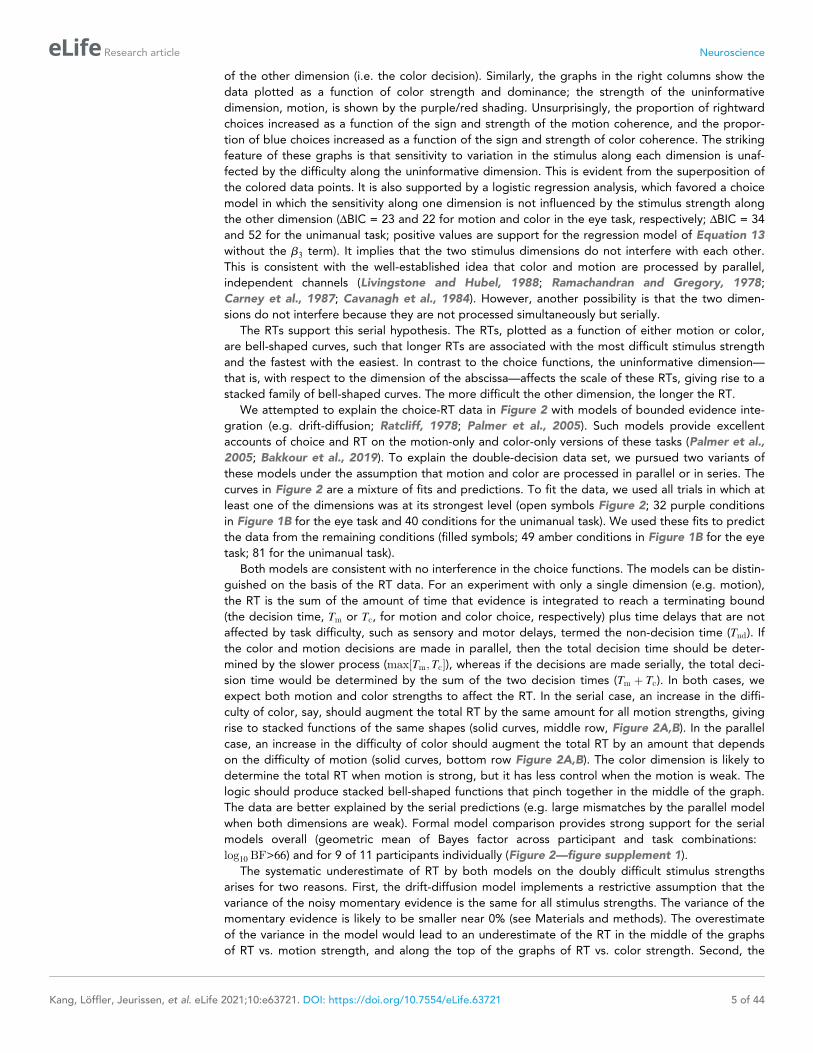
of the other dimension (i.e. the color decision). Similarly, the graphs in the right columns show the

data plotted as a function of color strength and dominance; the strength of the uninformative

dimension, motion, is shown by the purple/red shading. Unsurprisingly, the proportion of rightward

choices increased as a function of the sign and strength of the motion coherence, and the propor-

tion of blue choices increased as a function of the sign and strength of color coherence. The striking

feature of these graphs is that sensitivity to variation in the stimulus along each dimension is unaf-

fected by the difficulty along the uninformative dimension. This is evident from the superposition of

the colored data points. It is also supported by a logistic regression analysis, which favored a choice

model in which the sensitivity along one dimension is not influenced by the stimulus strength along

the other dimension (DBIC = 23 and 22 for motion and color in the eye task, respectively; DBIC = 34

and 52 for the unimanual task; positive values are support for the regression model of Equation 13

without the b3 term). It implies that the two stimulus dimensions do not interfere with each other.

This is consistent with the well-established idea that color and motion are processed by parallel,

independent channels (Livingstone and Hubel, 1988; Ramachandran and Gregory, 1978;

Carney et al., 1987; Cavanagh et al., 1984). However, another possibility is that the two dimen-

sions do not interfere because they are not processed simultaneously but serially.

The RTs support this serial hypothesis. The RTs, plotted as a function of either motion or color,

are bell-shaped curves, such that longer RTs are associated with the most difficult stimulus strength

and the fastest with the easiest. In contrast to the choice functions, the uninformative dimension—

that is, with respect to the dimension of the abscissa—affects the scale of these RTs, giving rise to a

stacked family of bell-shaped curves. The more difficult the other dimension, the longer the RT.

We attempted to explain the choice-RT data in Figure 2 with models of bounded evidence inte-

gration (e.g. drift-diffusion; Ratcliff, 1978; Palmer et al., 2005). Such models provide excellent

accounts of choice and RT on the motion-only and color-only versions of these tasks (Palmer et al.,

2005; Bakkour et al., 2019). To explain the double-decision data set, we pursued two variants of

these models under the assumption that motion and color are processed in parallel or in series. The

curves in Figure 2 are a mixture of fits and predictions. To fit the data, we used all trials in which at

least one of the dimensions was at its strongest level (open symbols Figure 2; 32 purple conditions

in Figure 1B for the eye task and 40 conditions for the unimanual task). We used these fits to predict

the data from the remaining conditions (filled symbols; 49 amber conditions in Figure 1B for the eye

task; 81 for the unimanual task).

Both models are consistent with no interference in the choice functions. The models can be distin-

guished on the basis of the RT data. For an experiment with only a single dimension (e.g. motion),

the RT is the sum of the amount of time that evidence is integrated to reach a terminating bound

(the decision time, Tm or Tc, for motion and color choice, respectively) plus time delays that are not

affected by task difficulty, such as sensory and motor delays, termed the non-decision time (Tnd). If

the color and motion decisions are made in parallel, then the total decision time should be deter-

mined by the slower process (max½Tm; Tc�), whereas if the decisions are made serially, the total deci-

sion time would be determined by the sum of the two decision times (Tm þ Tc). In both cases, we

expect both motion and color strengths to affect the RT. In the serial case, an increase in the diffi-

culty of color, say, should augment the total RT by the same amount for all motion strengths, giving

rise to stacked functions of the same shapes (solid curves, middle row, Figure 2A,B). In the parallel

case, an increase in the difficulty of color should augment the total RT by an amount that depends

on the difficulty of motion (solid curves, bottom row Figure 2A,B). The color dimension is likely to

determine the total RT when motion is strong, but it has less control when the motion is weak. The

logic should produce stacked bell-shaped functions that pinch together in the middle of the graph.

The data are better explained by the serial predictions (e.g. large mismatches by the parallel model

when both dimensions are weak). Formal model comparison provides strong support for the serial

models overall (geometric mean of Bayes factor across participant and task combinations:

log10 BF>66) and for 9 of 11 participants individually (Figure 2—figure supplement 1).

The systematic underestimate of RT by both models on the doubly difficult stimulus strengths

arises for two reasons. First, the drift-diffusion model implements a restrictive assumption that the

variance of the noisy momentary evidence is the same for all stimulus strengths. The variance of the

momentary evidence is likely to be smaller near 0% (see Materials and methods). The overestimate

of the variance in the model would lead to an underestimate of the RT in the middle of the graphs

of RT vs. motion strength, and along the top of the graphs of RT vs. color strength. Second, the




inclusion of all trials at 0% coherence tends to inflate the mean RT because just under half of the tri-

als resemble errors in the sense that the choice is opposite the sign of the component of the drift

rate that instantiates a direction or color bias (e.g. s0m 6¼ 0, Equation 2). Importantly, we pursued a

second approach to compare serial and parallel models which shows that the superiority of the serial

model does not rest on the systematic underestimates of RT in Figure 2.

In the second approach, we focus specifically on the decision times. It considers only the distribu-

tion of RTs and attempts to account for them under serial and parallel logic. Instead of fitting diffu-

sion models, this empirical approach explains the observed double-decision RT distributions as

either the serial or parallel combination of latent (i.e. unobservable) distributions of color and motion

decision times, as well as the four Tnd distributions (one for each choice). We estimate these latent

distributions with gamma distributions. For the serial case, the predicted double-decision RT distri-

butions are established by convolution of the latent single-dimension distributions and the distribu-

tion of Tnd. For the parallel case, the latent distributions are combined using the max logic, and the

result is convolved with the appropriate distribution of Tnd (see Materials and methods). Figure 2—

figure supplement 2 shows fits to the double-decision RT distributions for the more informative

conditions for the serial and parallel models. The model comparisons, based on all the data, yield

‘decisive’ support (Kass and Raftery, 1995) for the serial processing of motion and color (geometric

mean of Bayes factor for participant and task combinations log10 BF>17 with all but one out of 11

participants individually supporting the serial rule; Figure 2—figure supplement 3). We also display

the mean RTs derived from the fits in the same format as Figure 2 (Figure 2—figure supplement 4

and Figure 2—figure supplement 5). Both approaches support the conclusion that the color-motion

double-decisions are formed serially from two independent decision processes, each with its own

termination rule. However, neither analysis discerns the nature of the serial processing (e.g. whether

they alternate or one is prioritized). We will consider this issue later.

Experiment 2. Brief stimulus presentation (eye)The results from the double-decision RT experiment support sequential updating of two decision

variables, which represent accumulated evidence for the motion and color choices. If this is true, it

leads to a straightforward prediction. If the stimulus duration is not controlled by the decision maker

but by the experimenter, and if it is brief, then the two stimulus dimensions would compete for the

limited processing time, and we ought to observe choice-interference. We therefore conducted a

second experiment with the participants from Exp. 1-eye (N = 3). In this experiment, we presented

the same motion/color coherence combinations, but limited the duration of the stimulus viewing

time to just 120 ms. We know from previous experiments with 1D tasks that performance continues

to increase with stimulus duration up to at least one half second (Kiani et al., 2008; Waskom and

Kiani, 2018). Thus, it is reasonable to assume that performance accuracy would suffer if it is not pos-

sible to make use of the full 120 ms of evidence for both motion and color. We predicted that sensi-

tivity to both color and motion should be worse on the double-decision task than on color-only and

motion-only versions of the identical task. Each participant performed a total of 7305–7741 trials

(4052–4275 1D trials and 3240–3466 2D trials) over 12–19 days.

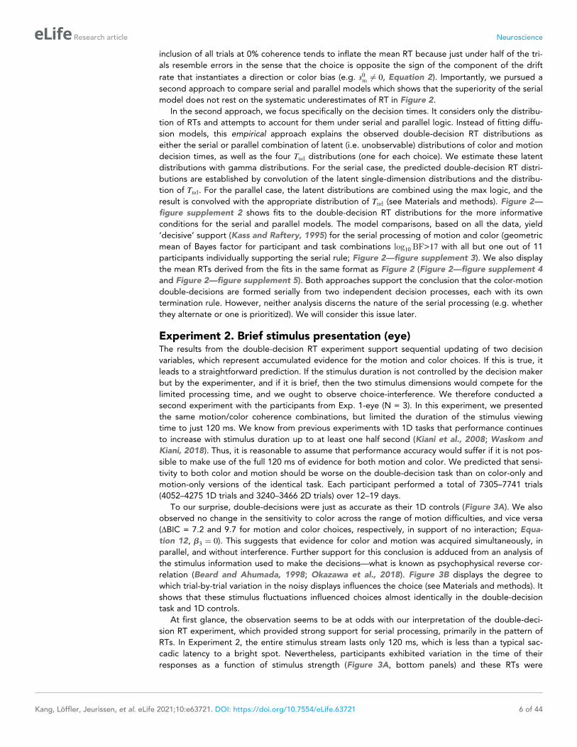
To our surprise, double-decisions were just as accurate as their 1D controls (Figure 3A). We also

observed no change in the sensitivity to color across the range of motion difficulties, and vice versa

(DBIC = 7.2 and 9.7 for motion and color choices, respectively, in support of no interaction; Equa-

tion 12, b3 ¼ 0). This suggests that evidence for color and motion was acquired simultaneously, in

parallel, and without interference. Further support for this conclusion is adduced from an analysis of

the stimulus information used to make the decisions—what is known as psychophysical reverse cor-

relation (Beard and Ahumada, 1998; Okazawa et al., 2018). Figure 3B displays the degree to

which trial-by-trial variation in the noisy displays influences the choice (see Materials and methods). It

shows that these stimulus fluctuations influenced choices almost identically in the double-decision

task and 1D controls.

At first glance, the observation seems to be at odds with our interpretation of the double-deci-

sion RT experiment, which provided strong support for serial processing, primarily in the pattern of

RTs. In Experiment 2, the entire stimulus stream lasts only 120 ms, which is less than a typical sac-

cadic latency to a bright spot. Nevertheless, participants exhibited variation in the time of their

responses as a function of stimulus strength (Figure 3A, bottom panels) and these RTs were




surprisingly long. The fastest were ~300 ms longer than the stimulus (RT>400 ms). Importantly, they

are approximately 100–200 ms longer in the double-decisions than in single decisions. It is difficult

to make too much of this observation, because the participants might have procrastinated for rea-

sons unrelated to the dynamics of the decision process. However, procrastination would not explain

the difference between the two conditions. As parallel acquisition of the 120 ms color and motion

take the same amount of time as acquisition of either of the streams alone (by definition), the extra

time in the double-decision is probably explained by serial incorporation of evidence into the two

decisions. This observation also implies the existence of buffers that store the information from one

stream as it awaits incorporation into the decision.

Our results so far suggest that color and motion information are acquired in parallel but are incor-

porated into the decision in series. We therefore wondered if the same schema might apply to the

double-decision RT task. For this to hold, some kind of alternation must occur such that segments of

one or the other stimulus stream is not incorporated into its decision. Suppose, for example, that at

t ¼ 120 ms, motion information had been incorporated into decision variable, Vm, and color informa-

tion had been stored in a buffer. Suppose further that motion continues to update the decision

A Brightward

choices

leftward

choices

blue

choices

yellow

choices

Exce

ss

mo

tio

n

for

rig

htw

ard

(a.u

.)

Exce

ss

co

lor

for

blu

e(a

.u.)

0

0.5

1

Pro

port

ion

rightw

ard

choic

es

0

0.5

1

Pro

port

ion

blu

e choic

es

single decision task

double decision task

-0.5 0 0.5


0.4

0.5

0.6

0.7

0.8

Response

tim

e(s

)

-0.5 0 0.5


0.4

0.5

0.6

0.7

0.8R

esponse

tim

e(s

)

Figure 3. Parallel acquisition and serial incorporation of a brief color-motion pulse (Experiment 2). Participants completed a short-duration variant of

the double-decision task in which the stimulus was presented for only 120 ms. They also performed blocks in which they were asked to report only the

color or only the motion direction (single decision in which they could ignore the irrelevant dimension). Data from double- and single-decision blocks

are indicated by color. (A) Choices and RTs for single and double-decision blocks. Top-left, proportion of rightward choices as a function of motion

strength. Top-right, proportion of blue choices as a function of color strength. The solid lines are logistic fits. They are nearly identical for single- and

double-decisions. Bottom row, RT for the single- and double-decisions plotted as a function of motion strength (left) and color strength (right). For

double-decisions, these are the same data plotted as a function of either the motion or color dimension. Data points show the average RT as a function

of motion or color coherence, after grouping trials across participants and all strengths of the ‘other’ dimension (i.e. color, left; motion, right). Error bars

indicate s.e.m. across trials. Although the stimulus was presented for only 120 ms, RTs were modulated by decision difficulty. Importantly, RTs were

longer in the double-decision task than in the single-decision task. (B) Psychophysical reverse correlation analysis. Top, Time course of the motion

information favoring rightward, extracted from the random-dot display on each trial, that gave rise to a left or right choice. Shading indicates s.e.m.

Middle, Time course of the color information favoring blue, extracted from the random-dot display on each trial, that gave rise to a blue or yellow

choice. Shading indicates s.e.m. The similarity of the green and orange curves indicates that participants were able to extract the same amount of

information from the stimulus when making single- and double-decisions. Bottom, Impulse response of the filters used to extract the motion and color

signals (see Materials and methods). They explain the long time course of the traces for the 120 ms duration pulse.




variable, Vm, until it reaches a termination bound at t ¼ Tm, and only then can the buffered color

information be incorporated into decision variable, Vc. From then on color information could update

Vc until this decision terminates. In this imagined scenario, the color information between 0.12 s and

Tm is not incorporated in the decision.

One might also imagine two alternatives to the latter part of this scenario. In both, the informa-

tion from color continues to update the buffer (but not Vc) throughout the motion decision without

loss. Then at t ¼ Tm either (i) all the information about color is incorporated immediately into Vc or

(ii) the buffered information is incorporated in Vc over time (e.g. as if the recorded color information

is played back). The first alternative is equivalent to the parallel model that is inconsistent with the

data. The second alternative, implausible as it may seem, implies the color decision is blind to the

color information in the display during the playback of the recorded color information. These alter-

natives are not intended as serious models but to convey two general intuitions. First, if there is a

buffer at play in the double-decision RT task then it must take time for the buffered information to

be incorporated, or the RTs would have conformed to the parallel logic. Second, if the duration of

the buffer is finite, when both 1D processes require more processing time than the duration of the

buffer, there will be portions of the color and/or motion stimulus that do not affect the decision.

One might therefore ask why the second point does not lead to a reduction in sensitivity (or accu-

racy) in color, say, when motion is weak and competes with color for processing time. The answer is

that when the decision maker controls the termination of the decision, they can compensate for the

missing information by collecting more, until the level reaches the same terminating bound. This

leads to a straightforward prediction. If the experimenter controls the termination of the evidence

stream, then missing portions of the color and/or motion stimulus might impair performance, espe-

cially when the other stimulus dimension is weak.

Experiment 3. Variable-duration stimulus presentation (eye)We therefore predicted that under conditions in which the experimenter controls the viewing dura-

tion, there is an intermediate range of viewing durations, greater than 120 ms and less than the aver-

age RT of difficult double-decisions, where we might observe interference in sensitivity. To

appreciate this prediction, it is essential to recognize that when the experimenter controls viewing

duration of a random dot display, the decision maker applies a termination criterion, as they do in

choice-RT experiments (Kiani et al., 2008). There is no overt manifestation of this termination,

although it can be identified by introducing perturbations to the stimulus (see also Kang et al.,

2017). Before such termination, sensitivity improves by the square root of the stimulus viewing dura-

tion (ffiffi

tp

) as expected for perfect integration of signal-plus-noise. In a double-decision, when the two

decision processes are splitting the time equally, the sensitivity of each should only improve byffiffiffiffiffiffiffi

t=2p

. However, when one process terminates, the rate of improvement of the other process should

recover, until that process reaches its terminating bound. The model predicts a range of stimulus

strengths and viewing durations in which interference in accuracy ought to be evident. It also pre-

dicts that the range and degree of interference might depend on which stimulus dimension the par-

ticipant prioritizes. Here, we set out to test this prediction.

Two participants each performed ~11,800 trials over 12–16 sessions. The task was identical in

structure to the brief-duration experiment. However, stimuli were presented at fixed durations rang-

ing from 120 to 1200 ms (in steps of 120 ms). Only three levels of difficulty were used for each

dimension: one easy and two difficult coherence levels. The two difficult coherence levels were

adjusted individually to yield 80% and 65% accuracy, respectively, ensuring above-chance perfor-

mance despite the high difficulty level. The easy coherence level was fixed at the highest motion/

color coherence from Experiment 1-unimanual, as this coherence typically supports perfect accuracy.

The number of coherence levels was reduced compared to Experiments 1 and 2 in light of the large

number of conditions (6 signed motion coherences � 6 signed color coherences � 10 stimulus dura-

tions). The key comparison here is sensitivity to difficult color, say, when (i) motion is difficult and

therefore likely to compete with the color for decision time vs. (ii) motion is easy and less likely to

wrest time away from color. This comparison within the double-decision task is more appropriate

than a comparison between the double and single decision tasks as these tasks are likely to elicit dif-

ferent termination bounds, as they have different error rates—0.75 and 0.5—on difficult trials (see

Materials and methods).




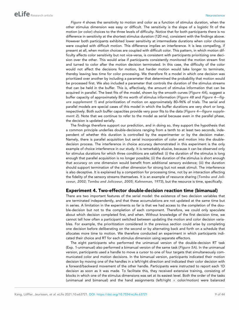
Figure 4 shows the sensitivity to motion and color as a function of stimulus duration, when the

other stimulus dimension was easy or difficult. The sensitivity is the slope of a logistic fit of the

motion (or color) choices to the three levels of difficulty. Notice that for both participants there is no

difference in sensitivity at the shortest stimulus duration (120 ms), consistent with the findings above.

However both participants exhibited lower sensitivity at intermediate durations when color choices

were coupled with difficult motion. This difference implies an interference. It is less compelling, if

present at all, when motion choices are coupled with difficult color. This pattern, in which motion dif-

ficulty affects color sensitivity but not vice-versa, is consistent with participants prioritizing one deci-

sion over the other. This would arise if participants consistently monitored the motion stream first

and turned to color after the motion decision terminated. In this case, the difficulty of the color

would not affect the decisions for motion, but harder motion would take longer to terminate,

thereby leaving less time for color processing. We therefore fit a model in which one decision was

prioritized over another by including a parameter that determined the probability that motion would

be processed first. We also included a parameter that controls the duration of the stimulus streams

that can be held in the buffer. This is, effectively, the amount of stimulus information that can be

acquired in parallel. The best fits of the model, shown by the smooth curves (Figure 4A), suggest a

buffer capacity of approximately 80 ms worth of stimulus information (Figure 4B and Figure 4—fig-

ure supplement 1) and prioritization of motion on approximately 80–96% of trials. The serial and

parallel models are special cases of this model in which the buffer durations are very short or long,

respectively. Both such buffer capacities provide very poor fits to the data (Figure 4—figure supple-

ment 2). Note that we continue to refer to the model as serial because even in the parallel phase,

the decision is updated serially.

The findings therefore support our prediction, and in doing so, they support the hypothesis that

a common principle underlies double-decisions ranging from a tenth to at least two seconds, inde-

pendent of whether this duration is controlled by the experimenter or by the decision maker.

Namely, there is parallel acquisition but serial incorporation of color and motion into the double-

decision process. The interference in choice accuracy demonstrated in this experiment is the only

example of choice interference in our study. It is remarkably elusive, because it can be observed only

for stimulus durations for which three conditions are satisfied: (i) the duration of the stimulus is long

enough that parallel acquisition is no longer possible; (ii) the duration of the stimulus is short enough

that accuracy on one dimension would benefit from additional sensory evidence; (iii) the duration

should support termination of the other dimension for strong but not weak stimuli. The interference

is also deceptive. It is explained by a competition for processing time, not by an interaction affecting

the fidelity of the sensory streams themselves. It is an example of resource sharing (Tombu and Joli-

coeur, 2002; Tombu and Jolicoeur, 2005; Kahneman, 1973), but the resource is time, specifically.

Experiment 4. Two-effector double-decision reaction time (bimanual)There are two important features of the serial model: the existence of two decision variables that

are terminated independently, and that these accumulations are not updated at the same time but

in series. A limitation in the experiments so far is that we had access to the completion of the dou-

ble-decision but not to the completion of each component. Therefore, we could only speculate

about which decision completed first, and when. Without knowledge of the first decision time, we

cannot tell how often a participant switched between updating the motion and color decision varia-

bles. For example, the prioritization considered in the previous section could arise by completing

one decision before deliberating on the second or by alternating back and forth on a schedule that

allocates more time to motion. We therefore conducted an experiment in which participants indi-

cated their choice and RT for each stimulus dimension using separate effectors.

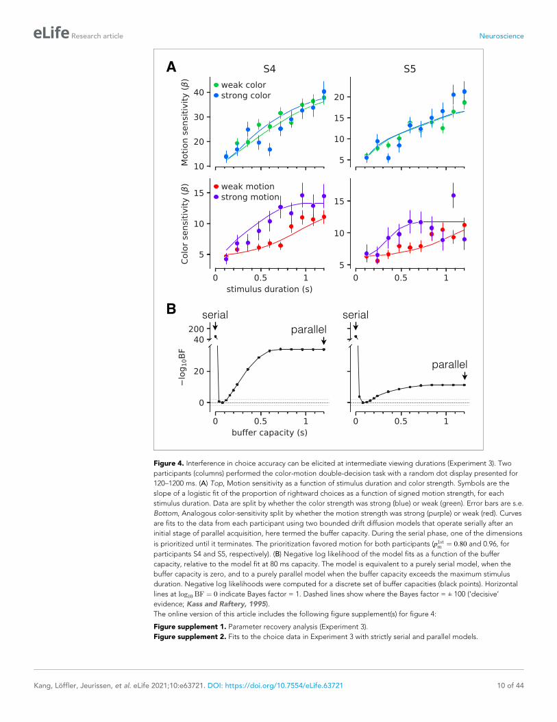
The eight participants who performed the unimanual version of the double-decision RT task

(Exp. 1-unimanual) also performed a bimanual version of the same task (Figure 5A). In the unimanual

version, participants used a handle to move a cursor to one of four targets that simultaneously com-

municated color and motion decisions. In the bimanual version, participants indicated their motion

decision by moving one of the handles in a left/right direction and indicated their color decision with

a forward/backward movement of the other handle. Participants were instructed to report each 1D

decision as soon as it was made. To facilitate this, they received extensive training, consisting of

blocks in which one of the stimulus dimensions was set at its easiest level. Both the order of the tasks

(unimanual and bimanual) and the hand assignments (left/right � color/motion) were balanced




parallel

A

B

parallel

serial serial

Figure 4. Interference in choice accuracy can be elicited at intermediate viewing durations (Experiment 3). Two

participants (columns) performed the color-motion double-decision task with a random dot display presented for

120–1200 ms. (A) Top, Motion sensitivity as a function of stimulus duration and color strength. Symbols are the

slope of a logistic fit of the proportion of rightward choices as a function of signed motion strength, for each

stimulus duration. Data are split by whether the color strength was strong (blue) or weak (green). Error bars are s.e.

Bottom, Analogous color-sensitivity split by whether the motion strength was strong (purple) or weak (red). Curves

are fits to the data from each participant using two bounded drift diffusion models that operate serially after an

initial stage of parallel acquisition, here termed the buffer capacity. During the serial phase, one of the dimensions

is prioritized until it terminates. The prioritization favored motion for both participants (p1stm ¼ 0:80 and 0.96, for

participants S4 and S5, respectively). (B) Negative log likelihood of the model fits as a function of the buffer

capacity, relative to the model fit at 80 ms capacity. The model is equivalent to a purely serial model, when the

buffer capacity is zero, and to a purely parallel model when the buffer capacity exceeds the maximum stimulus

duration. Negative log likelihoods were computed for a discrete set of buffer capacities (black points). Horizontal

lines at log10 BF ¼ 0 indicate Bayes factor = 1. Dashed lines show where the Bayes factor = ± 100 (‘decisive’

evidence; Kass and Raftery, 1995).


Figure supplement 1. Parameter recovery analysis (Experiment 3).

Figure supplement 2. Fits to the choice data in Experiment 3 with strictly serial and parallel models.




between the participants (see Materials and methods). Trial numbers (2304) and motion-color coher-

ence levels (11 � 11 combinations of signed coherence levels) were identical for the uni- and biman-

ual version of the task.

Before tackling the questions that motivate the bimanual experiment, we first ascertained

whether participants used the same strategy to make bimanual double-decisions as they did on the

unimanual version. It seemed conceivable that by using separate hands to indicate the motion and

color decisions, participants could achieve parallel decision formation, for example, as a pianist reads

the treble and bass staves with the right and left hands, typically. We therefore conducted a model

comparison similar to that of Figure 2. To fit the models, we used the color and motion choice on

each trial along with the second response time (RT2nd) regardless of whether it was to indicate

Figure 5. Replication of double-decision choice-reaction time when the decisions are reported with two effectors (Experiment 4). (A) Participants

performed the color-motion double-decision choice-reaction task, but indicated the double-decision with either a unimanual movement to one of four

choice-targets or a bimanual movement in which each hand reports one of the stimulus dimensions (N = 8 participants performed both tasks in a

counterbalanced order). In both conditions, the hand or hands were constrained by a robotic interface to move only in directions relevant for choice

(rectangular channels). The display was the same in the unimanual and bimanual tasks, with up-down movement reflecting color choice and left-right

movement reflecting motion choice. A scrolling display of proportion correct was used to encourage accuracy. In the unimanual trials both choices

were indicated simultaneously. However, in the bimanual trials each choice could be indicated separately and the dot display disappeared only when

the second hand left the home position. (B) Choice proportions and double-decision mean RT on the bimanual task. The double-decision RT on the

bimanual task is the latter of the two hand movements. The data are plotted as a function of either signed motion or color strength (abscissae), with the

other dimension shown by color (same conventions as in Figure 2). Solid traces are identical to the ones shown in Figure 2B for the unimanual task,

generated by the method of fitting the conditions containing at least one stimulus condition at its maximum strength and predicting the rest of the

data. They establish predictions for the bimanual data from the same participants. The agreement supports the conclusion that the participants used

the same strategy to solve the bimanual and unimanual versions of the task. Note that a few symbols are occluded by others.


Figure supplement 1. Choice and double-decision RT for the bimanual responses (Experiment 4) in the same format as Figure 2B.

Figure supplement 2. Model-free comparison of performance in the unimanual (blue) vs. bimanual (red) task (Experiment 4).




direction or color. This allows us to fit models that are identical to those used in the unimanual task

(Figure 2). In the bimanual task, the final RTs (RT2nd) are well described by the fits to the unimanual

double-decision RTs (Figure 5). We illustrate this in two ways. In the figure, the solid traces are not

fits to the bimanual data; they are fits to the unimanual data shown in Figure 2B. Clearly the choice

probabilities and RTs in the bimanual task are well captured by the model fit to the unimanual data.

The fits to the bimanual data are shown in Figure 5—figure supplement 1, and model comparison

favors the serial over the parallel model for seven of the eight participants (Figure 2—figure supple-

ment 1). Importantly, the participants’ behavior was strikingly similar in the unimanual and bimanual

versions of the task. The similarity between the two versions of the task is also supported with a

model-free analysis. In Figure 5—figure supplement 2, we superimpose the accuracy and the RTs

for the unimanual and bimanual tasks. There is an almost perfect overlap between these two aspects

of choice behavior, providing further support for a common set of processes operating in both ver-

sions of the task.

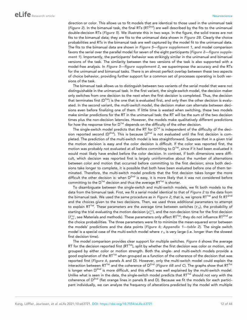
The bimanual task allows us to distinguish between two variants of the serial model that were not

distinguishable in the unimanual task. In the first variant, the single-switch model, the decision maker

only switches from one decision to the next when the first decision is completed. Thus, the decision

that terminates first (D1st) is the one that is evaluated first, and only then the other decision is evalu-

ated. In the second variant, the multi-switch model, the decision maker can alternate between deci-

sions even before finalizing one of them. If little time is wasted when switching, these two models

make similar predictions for the RT in the unimanual task: the RT will be the sum of the two decision

times plus the non-decision latencies. However, the models make qualitatively different predictions

for how the response time for D1st depends on the difficulty of the other decision.

The single-switch model predicts that the RT for D1st is independent of the difficulty of the deci-

sion reported second (D2nd). This is because D2nd is not evaluated until the first decision is com-

pleted. The prediction of the multi-switch model is less straightforward. Suppose that in a given trial

the motion decision is easy and the color decision is difficult. If the color was reported first, the

motion was probably not evaluated at all before committing to D1st, since if it had been evaluated it

would most likely have ended before the color decision. In contrast, if both dimensions were diffi-

cult, which decision was reported first is largely uninformative about the number of alternations

between color and motion that occurred before committing to the first decision; since both deci-

sions take longer to complete, it is possible that both have been evaluated before one of them ter-

minated. Therefore, the multi-switch model predicts that the first decision takes longer the more

difficult the other decision is: when D2nd is easy, it is more likely that it was not considered before

committing to the D1st decision and thus the average RT1st is shorter.

To disambiguate between the single-switch and multi-switch models, we fit both models to the

data from the bimanual task. First, we fit a serial model identical to that of Figure 2 to the data from

the bimanual task. We used the same procedure as in Figure 2; that is, we ignore RT1st and fit RT2nd

and the choices given to the two decisions. Then, we used three additional parameters to attempt

to explain RT1st. These parameters are the average time between switches (t D), the probability of

starting the trial evaluating the motion decision (p1stm ), and the non-decision time for the first decision

(T1stnd , see Materials and methods). These parameters only affect RT1st; they do not influence RT2nd or

the choice probabilities. The three parameters were fit to minimize the mean-squared error between

the models’ predictions and the data points (Figure 6; Appendix 1—table 2). The single switch

model is a special case of the multi-switch model where t D is very large (i.e. longer than the slowest

first decision time).

The model comparison provides clear support for multiple switches. Figure 6 shows the average

RT for the decision reported first (RT1st), split by whether the first decision was color or motion, and

grouped by either color or motion strength. Both the single- and multi-switch models provide a

good explanation of the RT1st when grouped as a function of the coherence of the decision that was

reported first (Figure 6, panels A and D). However, only the multi-switch model could explain the

interaction between RT1st and the coherence of D2nd (Figure 6B and C). The graphs show that RT1st

is longer when D2nd is more difficult, and this effect was well explained by the multi-switch model.

Unlike what is seen in the data, the single-switch model predicts that RT1st should not vary with the

coherence of D2nd (flat orange lines in panels B and D). Because we fit the models for each partici-

pant individually, we can analyze the frequency of alterations predicted by the model with multiple




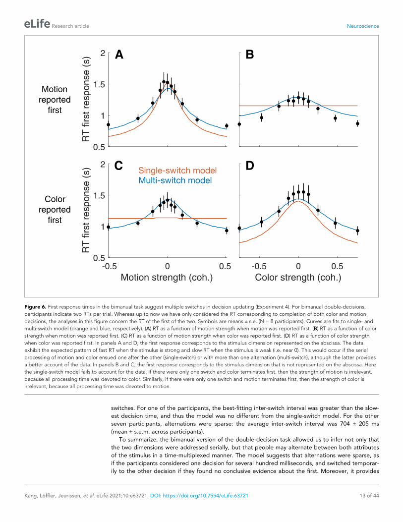
switches. For one of the participants, the best-fitting inter-switch interval was greater than the slow-

est decision time, and thus the model was no different from the single-switch model. For the other

seven participants, alternations were sparse: the average inter-switch interval was 704 ± 205 ms

(mean ± s.e.m. across participants).

To summarize, the bimanual version of the double-decision task allowed us to infer not only that

the two dimensions were addressed serially, but that people may alternate between both attributes

of the stimulus in a time-multiplexed manner. The model suggests that alternations were sparse, as

if the participants considered one decision for several hundred milliseconds, and switched temporar-

ily to the other decision if they found no conclusive evidence about the first. Moreover, it provides

0.5

1

1.5

2

RT

first

resp

on

se

(s) A B

-0.5 0 0.5


0.5

1

1.5

2

RT

first

resp

on

se

(s) C

-0.5 0 0.5


D

Color

reported

first

Motion

reported

first

Single-switch modelMulti-switch model

Figure 6. First response times in the bimanual task suggest multiple switches in decision updating (Experiment 4). For bimanual double-decisions,

participants indicate two RTs per trial. Whereas up to now we have only considered the RT corresponding to completion of both color and motion

decisions, the analyses in this figure concern the RT of the first of the two. Symbols are means ± s.e. (N = 8 participants). Curves are fits to single- and

multi-switch model (orange and blue, respectively). (A) RT as a function of motion strength when motion was reported first. (B) RT as a function of color

strength when motion was reported first. (C) RT as a function of motion strength when color was reported first. (D) RT as a function of color strength

when color was reported first. In panels A and D, the first response corresponds to the stimulus dimension represented on the abscissa. The data

exhibit the expected pattern of fast RT when the stimulus is strong and slow RT when the stimulus is weak (i.e. near 0). This would occur if the serial

processing of motion and color ensued one after the other (single-switch) or with more than one alternation (multi-switch), although the latter provides

a better account of the data. In panels B and C, the first response corresponds to the stimulus dimension that is not represented on the abscissa. Here

the single-switch model fails to account for the data. If there were only one switch and color terminates first, then the strength of motion is irrelevant,

because all processing time was devoted to color. Similarly, if there were only one switch and motion terminates first, then the strength of color is

irrelevant, because all processing time was devoted to motion.




direct evidence for two termination events, as assumed in our model fits. This rules out a class of

models of the double-decision as a race among four accumulations for each of the color-motion

combinations, what we term target-wise integration, as these models preclude completion of one

decision before the other.

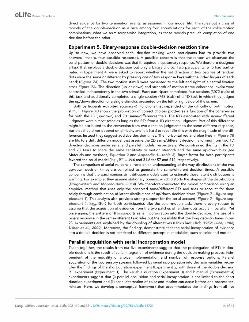
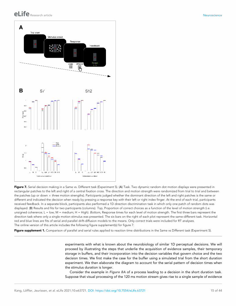
Experiment 5. Binary-response double-decision reaction timeUp to now, we have observed serial decision making when participants had to provide two

answers—that is, four possible responses. A possible concern is that the reason we observed the

serial pattern of double-decisions was that it required a quaternary response. We therefore designed

a task that involves a double-decision but only a binary choice. Two participants, who had partici-

pated in Experiment 4, were asked to report whether the net direction in two patches of random

dots were the same or different by pressing one of two response keys with the index fingers of each

hand; (Figure 7A). The two motion stimuli were presented to the left and right of a central fixation

cross Figure 7A. The direction (up or down) and strength of motion (three coherence levels) were

controlled independently in the two stimuli. Each participant completed four sessions (3072 trials) of

this task and additionally completed a single session (768 trials) of a 1D task in which they judged

the up/down direction of a single stimulus presented on the left or right side of the screen.

Both participants exhibited accuracy-RT functions that depended on the difficulty of both motion

stimuli. Figure 7B shows the proportion of correct choices plotted as a function of the coherences

for both the 1D (up-down) and 2D (same-difference) trials. The RTs associated with same-different

judgment were almost twice as long as the RTs from a 1D direction judgment. Part of this difference

might be attributed to the conversion from two direction judgments to the same-different response,

but that should not depend on difficulty and it is hard to reconcile this with the magnitude of the dif-

ference. Instead they suggest additive decision times. The horizontal red and blue lines in Figure 7B

are fits to a drift diffusion model that assume the 2D same/different decision is formed from two 1D

direction decisions under serial and parallel models, respectively. We constrained the fits in the 1D

and 2D tasks to share the same sensitivity to motion strength and the same up-down bias (see

Materials and methods, Equation 2 and Appendix 1—table 3). Bayes factor for both participants

favored the serial model (log10 BF ¼ 49:6 and 31.6 for S7 and S12, respectively).

The comparison of serial vs. parallel rests on an understanding of the way distributions of the two

up/down decision times are combined to generate the same/different decision times. A possible

concern is that the parsimonious drift diffusion models used to estimate these latent distributions is

wanting. For example, they assume stationary bounds, which distorts the shapes of the distributions

(Drugowitsch and Moreno-Bote, 2014). We therefore conducted the model comparison using an

empirical method that uses only the observed same/different RTs and tries to account for them

solely through combination of latent distributions of up/down decision times (Figure 7—figure sup-

plement 1). This analysis also provides strong support for the serial account (Figure 7—figure sup-

plement 1; log10 BF>7 for both participants). Like the color-motion task, there is every reason to

assume that the acquisition of evidence from the two patches of random dots occurs in parallel. Yet

once again, the pattern of RTs supports serial incorporation into the double decision. The use of a

binary response in the same-different task rules out the possibility that the long decision times in our

2D experiments are explained by the doubling of alternatives (Hick’s law; Hick, 1952; Luce, 1986;

Usher et al., 2002). Moreover, the findings demonstrate that the serial incorporation of evidence

into a double-decision is not restricted to different perceptual modalities, such as color and motion.

Parallel acquisition with serial incorporation modelTaken together, the results from our five experiments suggest that the prolongation of RTs in dou-

ble-decisions is the result of serial integration of evidence during the decision-making process, inde-

pendent of the modality of choice implementation and number of response options. Parallel

acquisition of the two sensory streams followed by serial incorporation into decision variables recon-

ciles the findings of the short duration experiment (Experiment 2) with those of the double-decision

RT experiment (Experiment 1). The variable duration (Experiment 3) and bimanual (Experiment 4)

experiments suggest that (i) parallel acquisition and serial incorporation is not limited to the short

duration experiment and (ii) serial alternation of color and motion can occur before one process ter-

minates. Here, we develop a conceptual framework that accommodates the findings from all five




experiments with what is known about the neurobiology of similar 1D perceptual decisions. We will

proceed by illustrating the steps that underlie the acquisition of evidence samples, their temporary

storage in buffers, and their incorporation into the decision variables that govern choice and the two

decision times. We first make the case for the buffer using a simulated trial from the short duration

experiment. We then elaborate the diagram to account for the serial pattern of decision times when

the stimulus duration is longer.

Consider the example in Figure 8A of a process leading to a decision in the short duration task.

Suppose that visual processing of the 120 ms motion stream gives rise to a single sample of evidence

Figure 7. Serial decision making in a Same vs. Different task (Experiment 5). (A) Task. Two dynamic random dot motion displays were presented in

rectangular patches to the left and right of a central fixation cross. The direction and motion strength were randomized from trial to trial and between

the patches (up or down � three motion strengths). Participants judged whether the dominant direction of the left and right patches is the same or

different and indicated the decision when ready by pressing a response key with their left or right index finger. At the end of each trial, participants

received feedback. In a separate block, participants also performed a 1D direction discrimination task in which only one patch of random dots was

displayed. (B) Results and fits for two participants (columns). Top, Proportion of correct choices as a function of the level of motion strength (i.e.

unsigned coherence; L = low; M = medium; H = High). Bottom, Response times for each level of motion strength. The first three bars represent the

direction task where only a single motion stimulus was presented. The six bars on the right of each plot represent the same-different task. Horizontal

red and blue lines are fits of serial and parallel drift-diffusion models to the means. Only correct trials were included for RT analyses.


Figure supplement 1. Comparison of parallel and serial rules applied to reaction time distributions in the Same vs Different task (Experiment 5).




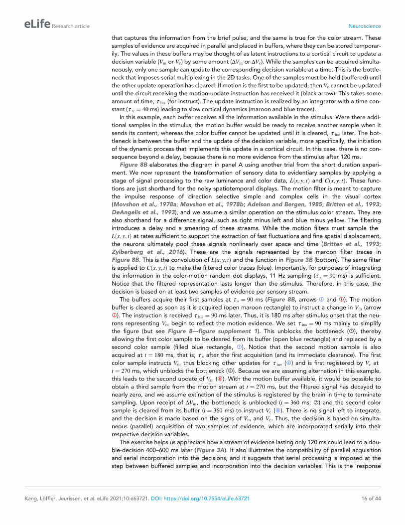
that captures the information from the brief pulse, and the same is true for the color stream. These

samples of evidence are acquired in parallel and placed in buffers, where they can be stored temporar-

ily. The values in these buffers may be thought of as latent instructions to a cortical circuit to update a

decision variable (Vm or Vc) by some amount (DVm or DVc). While the samples can be acquired simulta-

neously, only one sample can update the corresponding decision variable at a time. This is the bottle-

neck that imposes serial multiplexing in the 2D tasks. One of the samples must be held (buffered) until

the other update operation has cleared. If motion is the first to be updated, then Vc cannot be updated

until the circuit receiving the motion-update instruction has received it (black arrow). This takes some

amount of time, t ins (for instruct). The update instruction is realized by an integrator with a time con-

stant (t v ¼ 40ms) leading to slow cortical dynamics (maroon and blue traces).

In this example, each buffer receives all the information available in the stimulus. Were there addi-

tional samples in the stimulus, the motion buffer would be ready to receive another sample when it

sends its content, whereas the color buffer cannot be updated until it is cleared, t ins later. The bot-

tleneck is between the buffer and the update of the decision variable, more specifically, the initiation

of the dynamic process that implements this update in a cortical circuit. In this case, there is no con-

sequence beyond a delay, because there is no more evidence from the stimulus after 120 ms.

Figure 8B elaborates the diagram in panel A using another trial from the short duration experi-

ment. We now represent the transformation of sensory data to evidentiary samples by applying a

stage of signal processing to the raw luminance and color data, Lðx; y; tÞ and Cðx; y; tÞ. These func-

tions are just shorthand for the noisy spatiotemporal displays. The motion filter is meant to capture

the impulse response of direction selective simple and complex cells in the visual cortex

(Movshon et al., 1978a; Movshon et al., 1978b; Adelson and Bergen, 1985; Britten et al., 1993;

DeAngelis et al., 1993), and we assume a similar operation on the stimulus color stream. They are

also shorthand for a difference signal, such as right minus left and blue minus yellow. The filtering

introduces a delay and a smearing of these streams. While the motion filters must sample the

Lðx; y; tÞ at rates sufficient to support the extraction of fast fluctuations and fine spatial displacement,

the neurons ultimately pool these signals nonlinearly over space and time (Britten et al., 1993;

Zylberberg et al., 2016). These are the signals represented by the maroon filter traces in

Figure 8B. This is the convolution of Lðx; y; tÞ and the function in Figure 3B (bottom). The same filter

is applied to Cðx; y; tÞ to make the filtered color traces (blue). Importantly, for purposes of integrating

the information in the color-motion random dot displays, 11 Hz sampling (t s ¼ 90 ms) is sufficient.

Notice that the filtered representation lasts longer than the stimulus. Therefore, in this case, the

decision is based on at least two samples of evidence per sensory stream.

The buffers acquire their first samples at t s ¼ 90 ms (Figure 8B, arrows � and �). The motion

buffer is cleared as soon as it is acquired (open maroon rectangle) to instruct a change in Vm (arrow

�). The instruction is received t ins ¼ 90 ms later. Thus, it is 180 ms after stimulus onset that the neu-

rons representing Vm begin to reflect the motion evidence. We set t ins ¼ 90 ms mainly to simplify

the figure (but see Figure 8—figure supplement 1). This unblocks the bottleneck (�), thereby

allowing the first color sample to be cleared from its buffer (open blue rectangle) and replaced by a

second color sample (filled blue rectangle, �). Notice that the second motion sample is also

acquired at t ¼ 180 ms, that is, t s after the first acquisition (and its immediate clearance). The first

color sample instructs Vc, thus blocking other updates for t ins (�) and is first registered by Vc at

t ¼ 270 ms, which unblocks the bottleneck (�). Because we are assuming alternation in this example,

this leads to the second update of Vm (�). With the motion buffer available, it would be possible to

obtain a third sample from the motion stream at t ¼ 270 ms, but the filtered signal has decayed to

nearly zero, and we assume extinction of the stimulus is registered by the brain in time to terminate

sampling. Upon receipt of DVm, the bottleneck is unblocked (t ¼ 360 ms; �) and the second color

sample is cleared from its buffer (t ¼ 360 ms) to instruct Vc (�). There is no signal left to integrate,

and the decision is made based on the signs of Vm and Vc. Thus, the decision is based on simulta-

neous (parallel) acquisition of two samples of evidence, which are incorporated serially into their

respective decision variables.

The exercise helps us appreciate how a stream of evidence lasting only 120 ms could lead to a dou-

ble-decision 400–600 ms later (Figure 3A). It also illustrates the compatibility of parallel acquisition

and serial incorporation into the decisions, and it suggests that serial processing is imposed at the

step between buffered samples and incorporation into the decision variables. This is the ‘response




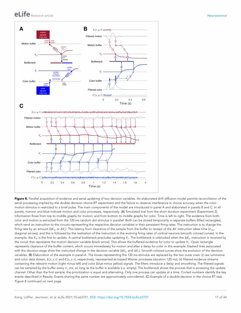
motion

sample

(120 ms)

updatebu er

Vm

clearbu er

update

(ΔVm)

color

sample

(120 ms)

updatebu er

Vc

clearbu er

update

(ΔVc)

updatechannel

unavailable

………………hold bu er

readyforupdate

B

C

A

Filtered motion

Motion buffer

0 0.2 0.4 0.6

Time (s)

Filtered color

Color buffer

Bottleneck

13

13

2 6

4 8

3 7

5

Filtered motion

Motion buffer

0 0.2 0.4 0.6 0.8 1 1.2 1.4 1.6 1.8 2

Time (s)

Filtered color

Color buffer

Bottleneck

1 3 5

13

7

2 6

4 8

3 7

5

Motion buffer

Color buffer

Bottleneck

Vm

Vc

Vm

Vc

Figure 8. Parallel acquisition of evidence and serial updating of two decision variables. An elaborated drift diffusion model permits reconciliation of the

serial processing implied by the double-decision choice-RT experiment and the failure to observe interference in choice accuracy when the color-

motion stimulus is restricted to a brief pulse. The main components of the model are introduced in panel A and elaborated in panels B and C. In all

panels, maroon and blue indicate motion and color processes, respectively. (A) Simulated trial from the short duration experiment (Experiment 2).

Information flows from top to middle graphs for motion; and from bottom to middle graphs for color. Time is left to right. The evidence from both

color and motion is extracted from the 120 ms random dot stimulus in parallel. Both can be stored temporarily in separate buffers (filled rectangles),

which send an instruction to the circuits representing the respective decision variables in their persistent firing rates. The instruction is to change the

firing rate by an amount (DVm or DVc). This latency from clearance of the sample from the buffer to receipt of the DV instruction takes time (t ins,

diagonal arrows), and this is followed by the realization of the instruction in the evolving firing rates of cortical neurons (smooth colored curves). In the

example, the Vm is the first to update. A central bottleneck precludes updating Vc. The bottleneck is unblocked when the DVm instruction is received by

the circuit that represents the motion decision variable (black arrow). This allows the buffered evidence for color to update Vc. Open rectangle

represents clearance of the buffer content, which occurs immediately for motion and after a delay for color in this example. Dashed lines associated

with the decision stage show the instructed change in the decision variable (DVm and DVc). Smooth colored curves show the evolution of the decision

variables. (B) Elaboration of the example in panel-A. The boxes representing the 120 ms stimulus are replaced by the two outer rows: (i) raw luminance

and color data stream, Lðx; y; tÞ and Cðx; y; tÞ, respectively, represented as biased Wiener processes (duration 120 ms); (ii) filtered evidence streams

containing the relevant motion (right minus left) and color (blue minus yellow) signals. The filters introduce a delay and smoothing. The filtered signals

can be sampled by the buffer every t s ms, so long as the buffer is available (i.e. empty). The bottleneck shows the process that is accessing the update

channel. Other than the first sample, the prioritization is equal and alternating. Only one process can update at a time. Circled numbers identify the key

events described in Results. Events sharing the same number are approximately coincidental. (C) Example of a double-decision in the choice-RT task.

Figure 8 continued on next page




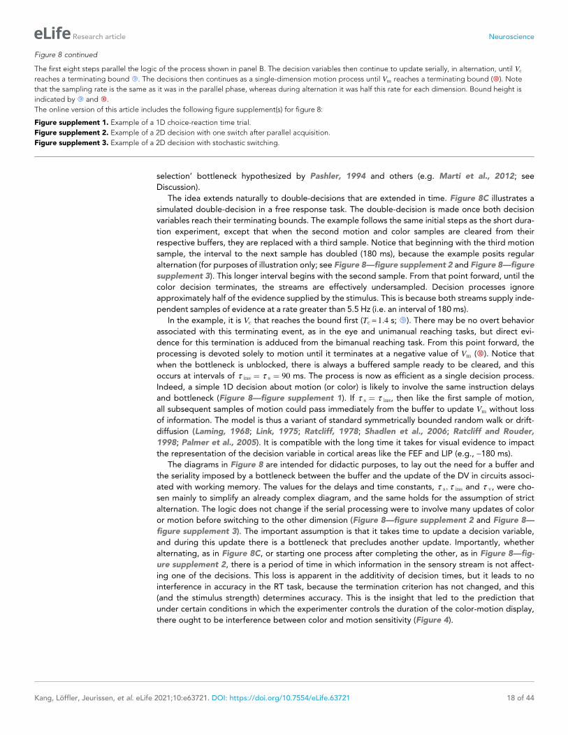
selection’ bottleneck hypothesized by Pashler, 1994 and others (e.g. Marti et al., 2012; see

Discussion).

The idea extends naturally to double-decisions that are extended in time. Figure 8C illustrates a

simulated double-decision in a free response task. The double-decision is made once both decision

variables reach their terminating bounds. The example follows the same initial steps as the short dura-

tion experiment, except that when the second motion and color samples are cleared from their

respective buffers, they are replaced with a third sample. Notice that beginning with the third motion

sample, the interval to the next sample has doubled (180 ms), because the example posits regular

alternation (for purposes of illustration only; see Figure 8—figure supplement 2 and Figure 8—figure

supplement 3). This longer interval begins with the second sample. From that point forward, until the

color decision terminates, the streams are effectively undersampled. Decision processes ignore

approximately half of the evidence supplied by the stimulus. This is because both streams supply inde-

pendent samples of evidence at a rate greater than 5.5 Hz (i.e. an interval of 180 ms).

In the example, it is Vc that reaches the bound first (Tc » 1:4 s; �). There may be no overt behavior

associated with this terminating event, as in the eye and unimanual reaching tasks, but direct evi-

dence for this termination is adduced from the bimanual reaching task. From this point forward, the

processing is devoted solely to motion until it terminates at a negative value of Vm (�). Notice that

when the bottleneck is unblocked, there is always a buffered sample ready to be cleared, and this

occurs at intervals of t ins ¼ t s ¼ 90 ms. The process is now as efficient as a single decision process.

Indeed, a simple 1D decision about motion (or color) is likely to involve the same instruction delays

and bottleneck (Figure 8—figure supplement 1). If t s ¼ t ins, then like the first sample of motion,

all subsequent samples of motion could pass immediately from the buffer to update Vm without loss

of information. The model is thus a variant of standard symmetrically bounded random walk or drift-

diffusion (Laming, 1968; Link, 1975; Ratcliff, 1978; Shadlen et al., 2006; Ratcliff and Rouder,

1998; Palmer et al., 2005). It is compatible with the long time it takes for visual evidence to impact

the representation of the decision variable in cortical areas like the FEF and LIP (e.g., ~180 ms).

The diagrams in Figure 8 are intended for didactic purposes, to lay out the need for a buffer and

the seriality imposed by a bottleneck between the buffer and the update of the DV in circuits associ-

ated with working memory. The values for the delays and time constants, t s; t ins and t v, were cho-

sen mainly to simplify an already complex diagram, and the same holds for the assumption of strict

alternation. The logic does not change if the serial processing were to involve many updates of color

or motion before switching to the other dimension (Figure 8—figure supplement 2 and Figure 8—

figure supplement 3). The important assumption is that it takes time to update a decision variable,

and during this update there is a bottleneck that precludes another update. Importantly, whether

alternating, as in Figure 8C, or starting one process after completing the other, as in Figure 8—fig-

ure supplement 2, there is a period of time in which information in the sensory stream is not affect-

ing one of the decisions. This loss is apparent in the additivity of decision times, but it leads to no

interference in accuracy in the RT task, because the termination criterion has not changed, and this

(and the stimulus strength) determines accuracy. This is the insight that led to the prediction that

under certain conditions in which the experimenter controls the duration of the color-motion display,

there ought to be interference between color and motion sensitivity (Figure 4).

Figure 8 continued

The first eight steps parallel the logic of the process shown in panel B. The decision variables then continue to update serially, in alternation, until Vc

reaches a terminating bound �. The decisions then continues as a single-dimension motion process until Vm reaches a terminating bound (�). Note

that the sampling rate is the same as it was in the parallel phase, whereas during alternation it was half this rate for each dimension. Bound height is

indicated by � and �.


Figure supplement 1. Example of a 1D choice-reaction time trial.

Figure supplement 2. Example of a 2D decision with one switch after parallel acquisition.

Figure supplement 3. Example of a 2D decision with stochastic switching.




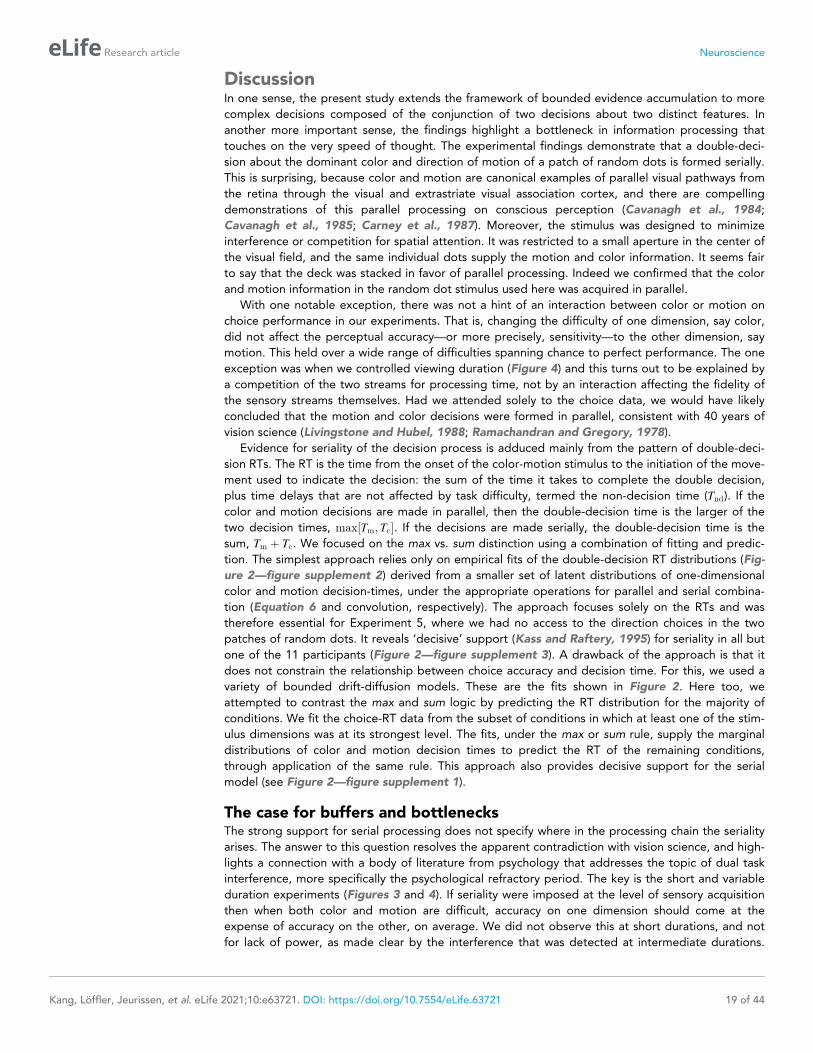
DiscussionIn one sense, the present study extends the framework of bounded evidence accumulation to more

complex decisions composed of the conjunction of two decisions about two distinct features. In

another more important sense, the findings highlight a bottleneck in information processing that

touches on the very speed of thought. The experimental findings demonstrate that a double-deci-

sion about the dominant color and direction of motion of a patch of random dots is formed serially.

This is surprising, because color and motion are canonical examples of parallel visual pathways from

the retina through the visual and extrastriate visual association cortex, and there are compelling

demonstrations of this parallel processing on conscious perception (Cavanagh et al., 1984;

Cavanagh et al., 1985; Carney et al., 1987). Moreover, the stimulus was designed to minimize

interference or competition for spatial attention. It was restricted to a small aperture in the center of

the visual field, and the same individual dots supply the motion and color information. It seems fair

to say that the deck was stacked in favor of parallel processing. Indeed we confirmed that the color

and motion information in the random dot stimulus used here was acquired in parallel.

With one notable exception, there was not a hint of an interaction between color or motion on

choice performance in our experiments. That is, changing the difficulty of one dimension, say color,

did not affect the perceptual accuracy—or more precisely, sensitivity—to the other dimension, say

motion. This held over a wide range of difficulties spanning chance to perfect performance. The one

exception was when we controlled viewing duration (Figure 4) and this turns out to be explained by

a competition of the two streams for processing time, not by an interaction affecting the fidelity of

the sensory streams themselves. Had we attended solely to the choice data, we would have likely

concluded that the motion and color decisions were formed in parallel, consistent with 40 years of

vision science (Livingstone and Hubel, 1988; Ramachandran and Gregory, 1978).

Evidence for seriality of the decision process is adduced mainly from the pattern of double-deci-

sion RTs. The RT is the time from the onset of the color-motion stimulus to the initiation of the move-

ment used to indicate the decision: the sum of the time it takes to complete the double decision,

plus time delays that are not affected by task difficulty, termed the non-decision time (Tnd). If the

color and motion decisions are made in parallel, then the double-decision time is the larger of the

two decision times, max½Tm; Tc�. If the decisions are made serially, the double-decision time is the

sum, Tm þ Tc. We focused on the max vs. sum distinction using a combination of fitting and predic-

tion. The simplest approach relies only on empirical fits of the double-decision RT distributions (Fig-

ure 2—figure supplement 2) derived from a smaller set of latent distributions of one-dimensional

color and motion decision-times, under the appropriate operations for parallel and serial combina-

tion (Equation 6 and convolution, respectively). The approach focuses solely on the RTs and was

therefore essential for Experiment 5, where we had no access to the direction choices in the two

patches of random dots. It reveals ‘decisive’ support (Kass and Raftery, 1995) for seriality in all but

one of the 11 participants (Figure 2—figure supplement 3). A drawback of the approach is that it

does not constrain the relationship between choice accuracy and decision time. For this, we used a

variety of bounded drift-diffusion models. These are the fits shown in Figure 2. Here too, we

attempted to contrast the max and sum logic by predicting the RT distribution for the majority of

conditions. We fit the choice-RT data from the subset of conditions in which at least one of the stim-

ulus dimensions was at its strongest level. The fits, under the max or sum rule, supply the marginal

distributions of color and motion decision times to predict the RT of the remaining conditions,

through application of the same rule. This approach also provides decisive support for the serial

model (see Figure 2—figure supplement 1).

The case for buffers and bottlenecksThe strong support for serial processing does not specify where in the processing chain the seriality

arises. The answer to this question resolves the apparent contradiction with vision science, and high-

lights a connection with a body of literature from psychology that addresses the topic of dual task

interference, more specifically the psychological refractory period. The key is the short and variable

duration experiments (Figures 3 and 4). If seriality were imposed at the level of sensory acquisition

then when both color and motion are difficult, accuracy on one dimension should come at the

expense of accuracy on the other, on average. We did not observe this at short durations, and not

for lack of power, as made clear by the interference that was detected at intermediate durations.




Nor did we observe any reduction in accuracy compared to single decisions, and there was no differ-

ence in the magnitude and time course over which momentary fluctuations of color and motion pre-

dicted the individual choices on single- and double-decisions (Figure 3B). These observation also

rule out the possibility that there was interference but it was balanced across trials—that is, a mixture

of trials in which successful motion processing impaired color processing on half the trials and suc-

cessful color processing impaired motion processing on the other half.

Thus, the short duration experiment demonstrates parallel processing and the necessity of at

least one buffer. The results in the variable duration experiment might lead us to entertain the possi-

bility that only color is buffered, because motion was prioritized. However, the bimanual task dem-

onstrates that motion is not always processed first, and both color and motion are processed before

the first process terminates. We therefore conclude that there are two buffers which are capable of

holding a sample of evidence about color or motion, respectively, while the other dimension is incor-

porated into the decision. This places the bottleneck between the buffered evidence and the repre-

sentation of the decision variable. We believe the bottleneck arises because of an anatomical

constraint. It is simply impossible to connect in parallel every possible source of evidence with the

neural circuits responsible for representing a proposition or plan. As Zylberberg et al., 2010 theo-

rized, the brain’s routing problem holds the key to why many mental operations operate serially. We

will return to this idea after interpreting our results in the context of the neurobiology of decision

making. We do this by pursuing the neural correlates of a computational model that supports paral-

lel acquisition of sensory evidence and its serial incorporation into two decisions.

Connecting computational models to neurobiologyThe operations depicted in Figure 8 are intended to reconcile what is known about the neurobiol-

ogy of simple 1D decisions with the constraints introduced by the double-decision task. The mathe-

matical instantiation of the model requires only minor modifications of two bounded drift-diffusion

processes with temporal multiplexing (see Materials and methods). However, the architecture

implied by Figure 8B,C facilitates interpretation of the experimental findings in relation to neural

processing. In the mathematical depiction of drift-diffusion, the momentary evidence is a biased

Wiener process. However, in reality the stimulus is not a Wiener process, nor is the representation of

momentary evidence by neurons (Zylberberg et al., 2016), which arise through application of a

transfer function that effectively spreads the impact of a pair of displaced dots over 100–150 ms

(Figure 3B, bottom; Adelson and Bergen, 1985). Thus, the neural representation of the motion can

be approximated by the leaky integral of a biased Wiener process (Cain et al., 2013; Barlow and

Tripathy, 1997). Such smoothing would not be warranted for the detection of fast changes, but it is

adequate for a signal that is to be integrated over time. We know less about the filtration of a color

difference, but the same logic applies.

The conceptual transition from Wiener processes to discrete samples allows us to appreciate the

similarity between the accumulation of evidence from movie-like stimuli and the broader class of deci-

sions based on discrete samples of evidence from the environment and memory. This informs hypoth-

eses about the neurobiology, because the sample of evidence ultimately bears on a decision in units of

belief or relative value. That is obvious when considering a choice between items on a menu, but it has

been camouflaged to some extent in the perceptual decision-making literature. This is in part because

the time-integral of a difference in firing rates from right- and left-preferring neurons is the number of

excess spikes for right, which is itself proportional to the accumulated log-likelihood ratio that this

excess was observed because motion was in fact rightward (Gold and Shadlen, 2001; Shadlen et al.,

2006; Beck et al., 2008). For the wider class of decisions, such difference variables are elusive,

whereas the possibility of associating a sample with log-likelihood is a natural dividend of learning and

memory (Yang and Shadlen, 2007; Kira et al., 2015; Shadlen and Shohamy, 2016).

The results imply the maintenance of separate decision variables each capable of reconciling deci-

sion and choice for the one stimulus dimension. There must be separate control of termination and

negligible cross talk. Specifically, the state of the accumulated evidence bearing on the direction of

motion does not affect the amount of accumulated evidence required to reach a decision about

color dominance, and the same can be said about the state of the accumulated evidence about color

on the decision about direction of motion. In the model the decision variables, Vm and Vc , represent

the integrated evidence for right (and against left) and for blue (and against yellow). Neural corre-

lates of these 1D processes are known, mainly in the parietal and prefrontal cortex (Gold and




Shadlen, 2007), although they are organized in pairs: R� L, L� R (and presumably B� Y and

Y � B). Each of the four processes is the accumulation of positive and negative increments, and each

is terminated by an upper bound. Because evidence for R and L are anticorrelated (likewise for B

and Y ), the pair of opposing processes is approximated by one-dimensional drift-diffusion to sym-

metric upper and lower terminating bounds. All model-fits adopt this approximation.

An alternative formulation, which we term target-wise integration, would accumulate evidence for

the pair of features associated with each choice target (e.g. RB, RY, LB, LY ). If such mechanism were

to terminate when the total accumulation reaches a threshold, it would predict a type of choice-

interference such that sensitivity to motion, say, would be impaired when the color strength was

high, because the decision time is shortened by the stronger stimulus. We have not pursued all var-

iants of target-wise integration, but critically, the bimanual experiment demonstrates that the dou-

ble-decision comprises two terminating events.

Integration as instructionWe find it useful to characterize integration as the implementation of a sequence of instructions to

increment and decrement persistent activity in cortical areas that represent the decision variables. In

Figure 8, the instructed change is realized by simple first order dynamics chosen to approximate

neural responses from area LIP. The implementation is merely phenomenological, but it jibes with

emerging ideas in theoretical neuroscience that characterize computation as a change in circuit con-

figuration to establish stable states and dynamics (Remington et al., 2018). For decision making, it

replaces the requirement for continuous integration, with the realization of instructions as if drawn

from a memory stage. This characterization also extends to the buffer.

Recall, the buffer was introduced to explain the observation that a brief pulse of color-motion,

acquired in parallel, appears to be incorporated into the decision serially. We characterized the

length of the buffer—its storage capacity—using the data from the variable duration experiment

(Figure 4), where we equate it with the duration of parallel acquisition. This is reasonable because

thereafter, the process is serial. However, this depiction appears to limit the role of the buffer to the

beginning of the decision, and it fails to specify how long the information can be held. If there are

alternations between color and motion processing before the first process terminates, as shown in

Figure 6, then information might be buffered beyond the initial parallel phase. As shown in

Figure 8C, during alternation a sample might be held for at least 2t ins—that is, the time it takes the

cleared sample to instruct the appropriate decision process and the time the bottleneck is in play

while the other dimension performs its update. If the alternations are less frequent, the buffer might

need to hold information longer, and if there is only one transition, then the buffer might be

expected to hold a sample of information for the duration of the entire first decision (e.g. Figure 8—

figure supplement 2). There is presumably a limit on how long a sample can be stored, but studies

of visual iconic memory suggest that a sample of evidence might be buffered for ~500 ms (Sperl-

ing, 1960; Gegenfurtner and Kiper, 1992).

We conceive of the buffer residing between the cortical areas that represent the filtered evidence

and other cortical circuits that represent the decision variables. Notice that the operations depicted in

Figure 8 assign two duties to the buffer: (i) storage of a sample of evidence while the bottleneck pre-

cludes updating the associated decision variable and (ii) conversion of the sample into an instruction

to update a decision variable by DV . These duties could be carried out by different circuits. An appeal-

ing candidate for both operations is the striatum. The striatum receives input from the extrastriate

visual cortex (Ding and Gold, 2012b), and it is known to play a role in connecting value to action selec-

tion (Hikosaka et al., 2014) as well as working memory (Akhlaghpour et al., 2016). In the context of

our results, we would characterize the operation as follows. A sample of filtered evidence, represented

by the firing rates of neurons in extrastriate cortex (e.g. areas MT/MST) leads to a change in the state

of a striatal circuit, such that its reactivation transmits the DV instruction to the cortical areas that rep-

resent the decision variables, and this takes time (t ins). On this view, the bottleneck is the striato-tha-

lamo-cortical pathway. There has been an observation of the bottleneck in a split-brain patient,

supporting such a subcortical bottleneck at least in certain instances (Pashler et al., 1994).

A second possibility is that the buffered evidence is stored in visual cortical association areas,

especially areas with persistent representations. For example, it has been suggested that short-term

visual iconic memory is supported by the slowly decaying spike rates of neurons in area V2

(O’Herron and von der Heydt, 2009) and the anterior superior temporal sulcus (STSa)




(Keysers et al., 2005). This would place the bottleneck between extrastriate cortex and the parietal

and prefrontal areas that represent the decision variable (see also Marti et al., 2012). This possibility

does not provide an explanation for why communication between these areas would impose a sub-

stantial delay (e.g. t ins).

A third possibility would identify the buffer with control circuitry within the very cortical areas that

represent the decision variables. This might seem far-fetched but there is evidence for such an oper-

ation in the premotor cortex of mice, where it underlies the implementation of the logical ‘exclusive

or’ (XOR) operation (Wu et al., 2020). In that case the bottleneck would be intracortical. It would

correspond to the implementation of a circuit state from its ‘silent’ representation—that is, in cellular

and subcellular (e.g. synaptic) states rather than persistent spike activity (Mongillo et al., 2008;

Lundqvist et al., 2018). The bottleneck is the conversion from this state to the establishment of the

spiking dynamics that instantiate the DV instruction. This might resemble the recall of an associative

memory, which must facilitate the establishment of cortical persistent activity in a state suitable for

computation, be it for further updating or comparison to a criterion. The three possibilities are not

mutually exclusive; nor are they exhaustive. In any case, the instigating event is the unblocking of the

bottleneck, signaled by the circuit that receives the DV instruction.

The bottleneckUp to now, we have alluded to the bottleneck as a temporary obstruction to color or motion process-

ing, but the bottleneck itself does not add time. It is the instructive step that takes time (t ins). This step

comprises the conversion of a sample of evidence to a DV instruction and its transmission to a cortical

circuit. Indeed, the same delay is encountered in simpler decisions. For example, in the 1D random

dot motion task, the incorporation of evidence into the neural representation of the decision variable

is first evident 80–100 ms after neurons in area MT exhibit direction selective responses (de Lafuente

et al., 2015; Ding and Gold, 2012a; Kim and Shadlen, 1999) and this delay holds for perturbations of

the stimulus throughout decision formation (Huk and Shadlen, 2005). This is too long to be explained

by synaptic latencies. It implies either a complex routing through intermediate structures or more

sophisticated processing that serves to facilitate the linkage and/or the conversion of the sample to an

instruction suitable for establishing the cortical dynamics that ultimately realize the DV instruction. The

delay corresponds to the sum, t s þ t ins (circles 1 and 2 in Figure 8).

Decision variables are represented in the persistent activity of neurons in the parietal and prefron-

tal cortex of primates. Such persistent activity is associated with working memory, attention and

planning. This functional localization conforms to the notion of a ‘response selection’ bottleneck

hypothesized by Harold Pashler to explain dual task interference (Pashler, 1994), in particular a phe-

nomenon known as the psychological refractory period (PRP): the prolonged latency of the second

of two adjacent decisions without an effect on accuracy. In his and our formulation, it reflects a limi-

tation that restricts the flow of information to affect higher processes such as decision-making and

short-term working memory. On initial consideration, there is no obvious reason why the formation

of working memory should necessitate a bottleneck. If acquisition can be parallel, why not working

memory or the formation of a provisional plan or intention?

Framed in the language of decision-making, seriality arises as a consequence of limited connectiv-

ity between the brain’s evidence acquisition systems—sensory, memory, and emotion—and the sys-

tems that represent information in an intentional frame of reference, that is, as provisional

affordances. Any possible intention might be informed by a variety of sources of evidence, which

may be acquired in parallel but from different locations in the brain. The brain lacks the anatomy to

support independent connections from all sources of evidence to all possible intentions—that is, the

circuits that represent them. Instead the communication must share connections, and this invites

some form of time-slice multiplexing. It is not possible for every source of evidence to communicate

with the circuits that form decisions at the same time. For some dedicated operations, it is likely that

many sources of ‘evidence’ do converge on the same intentional circuitry (e.g. escape response;

Evans et al., 2018; Lee et al., 2020), and the tracts can be established through development. But,

for flexible cognitive systems that learn and solve problems, the connections between evidence and

intention must be multipotent and malleable, since connecting N sources of evidence and M inten-

tions will need at least N �M wires if they are connected exhaustively, whereas if they are routed

centrally, it will only need N þM. This solution necessitates some type of multiplexing

(Zylberberg et al., 2010; Feng et al., 2014; Musslick et al., 2017).




Relation to cognitive tasksWe suspect that the constraints leading to serial processing in the color-motion task also apply to

other decisions and cognitive functions. For example, deciding between two familiar food items can

take a surprisingly long time when those items are valued similarly. This holds when the items are

both highly valued or both undesired or both of moderate value. Like decisions about the direction

of random dot motion, there is a lawful relationship between the RT to choose an item and the likeli-

hood that the preference is consistent with one’s previously stated value (Krajbich et al., 2010;

Krajbich and Rangel, 2011). Like the choice-RT accompanying 1D motion (or color) decisions, the

relationship suggests that some type of process like noisy evidence accumulation—or more gener-

ally, sequential sampling with optional stopping—reconciles choice and decision time. However,

such expressions of preference differ from perceptual decisions in two important ways. First, there is

no objectively correct response, only consistency with the sign of the inequality in the decision-mak-

er’s valuations of the individual items, which are ascertained before the experiment. Second, the

food items are not shown as a movie and there is no uncertainty about their identity. Therefore, it is

not clear what gives rise to independent samples of evidence. Bakkour et al., 2019 showed that the

samples are likely to arise through constructive processes using hippocampal memory systems. This

begs the question why this process would unfold in time like a movie of random dots. An attractive

idea is that the use of memory guided valuation—in particular the step to enable it to affect a deci-

sion variable—encounters a bottleneck. Even if memories could be retrieved in parallel, they would

require buffering and serial updates of the decision variable (Shadlen and Shohamy, 2016).

While it is unsurprising that a movie of random dots supplies evidence to be incorporated serially

toward a decision, it is shocking that two samples of evidence, supplied simultaneously by the same

dots and acquired through parallel sensory channels, do not support simultaneous decisions. In the

experiments that require prolonged viewing, non-simultaneity manifests in serial time-multiplexed

alternation of the decision processes and the failure to incorporate all information in the stimulus

stream into one or both decisions. In a free response design, the decision maker compensates by

acquiring more evidence, so the interference is not apparent in the accuracy of the perceptual

choice. However, if such compensation is precluded by the experimenter (variable duration experi-

ment), the failure to incorporate information can affect accuracy too. That this bottleneck arises

despite parallel acquisition of color and motion (or motion from two locations), whether we use one

or two effectors to express the decision, and whether we decide between 2 � 2 conjunctions or two

categories (same/different) suggests that the bottleneck is pervasive. In addition to the PRP, we sus-

pect that it plays a role in other psychological phenomena, such as post-stimulus masking, the atten-

tional blink (e.g. as shown in the rapid serial visual presentation tasks), and conjunction search

(Potter, 1976; Treisman and Gelade, 1980; Keysers and Perrett, 2002; Marti et al., 2015;

Marti and Dehaene, 2017). These phenomena represent forms of sequential interference and all

can be stated as challenges to the brain’s routing system (Zylberberg et al., 2010).

On the other hand, one must wonder if the brain can ever take advantage of parallel acquisition to

perform cognitive functions in parallel. It certainly seems so to a musician using their feet and hands to

convey time and sonority on a piano or polyrhythm on a drum kit. Yet the time scales of alternation dis-

cussed in this paper are on the order of 10 Hz. It seems possible that we achieve parallel processing

despite the bottleneck by enhancing signal-processing at the filter stage before the bottleneck and by

grouping (or chunking) processes after the bottleneck in higher order controllers of movement and

strategy. For example, face selective neurons compute conjunctions of features in less than 100 ms

(Freiwald and Tsao, 2010). This is just one example of the sophisticated properties of association sen-

sory neurons in the extrastriate visual cortex, and analogous operations are presumed to occur in sec-

ondary somatosensory cortex and belt regions of the auditory cortex (e.g. Bizley and Cohen, 2013;

Moses et al., 2016; Jiang et al., 1997). Similarly, complex movement sequences and the rules to coor-

dinate them may be specified in premotor cortex or at the level of the controller. If so, then the only

way to overcome the bottleneck is to develop the expertise of the reader or the musician/athlete, leav-

ing most of flexible cognition to negotiate the bottleneck between the acquisition of information and

its incorporation into representations that support states of knowledge: decisions, working memory,

plans of action. It is the price the brain pays to use its senses (and memory) to bear on a plethora of

possible intentions, despite its limited connectivity. The payment is in time, but in another sense, it is




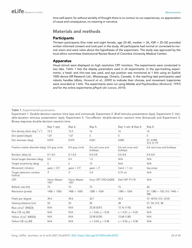
time well spent, for without seriality of thought there is no contour to our experiences, no appreciation

of cause and consequence, no meaning or narrative.

Materials and methods

ParticipantsThirteen participants (five male and eight female, age 23–40, median = 26, IQR = 25–32) provided

written informed consent and took part in the study. All participants had normal or corrected-to-nor-

mal vision and were naıve about the hypotheses of the experiment. The study was approved by the

local ethics committee (Institutional Review Board of Columbia University Medical Center).

ApparatusVisual stimuli were displayed on high resolution CRT monitors. The experiments were conducted in

two labs. Table 1 lists the display parameters used in all experiments. In the eye-tracking experi-

ments, a head- and chin-rest was used, and eye position was monitored at 1 kHz using an Eyelink

1000 device (SR Research Ltd., Mississauga, Ontario, Canada). In the reaching task participants used

robotic handles (vBots, Howard et al., 2009) to indicate their choices, and movement trajectories

were recorded at 1 kHz. The experiments were run using Matlab and Psychtoolbox (Brainard, 1997)

and for the online experiments jsPsych (de Leeuw, 2015).

Table 1. Experimental parameters.

Experiment 1. Double-decision reaction time (eye and unimanual), Experiment 2. Brief stimulus presentation (eye), Experiment 3. Vari-

able-duration stimulus presentation (eye), Experiment 4. Two-effector double-decision reaction time (bimanual) and Experiment 5.

Binary-response double-decision reaction time.

Exp 1.-eye Exp 2. Exp 3. Exp 1.-uni. & Exp 4. Exp 5.

Dot density (dots deg-2 s-1) 15.3 15.3 16 16 16

Dot speed (deg/s) 1.67 1.67 5 5 5

Dot diameter (deg) 0.075 0.075 0.061 0.082 S7: 0.098;S12: 0.119

Fixation marker diameter (deg) 0.4 gray circle 0.4 gray circle 0.6 red cross andbullseye

0.6 red cross andbullseye

0.6 red cross and bullseye

Random delay (s) 0.1–0.5 0.1–0.5 0.5–0.8 0.5–0.8 0.4–0.8

Visual target diameter (deg) 0.4 0.4 1.2 N/A N/A

Target eccentricity (deg) 6 6 15 N/A N/A

Movement initiation gaze > 2.5˚ gaze > 2.5˚ gaze > 3˚ hand > 1 cm key press

Target detection window(radius)

3˚ 3˚ 2.4˚ 0.75 cm N/A

CRT Vision Master1451

Vision Master1451

Sony CRT CPD-G420S Dell CRT P1110 N/A

Refresh rate (Hz) 75 75 75 75 60

Resolution (pixels) 1400 � 1050 1400 � 1050 1280 � 1024 1280 � 1024 S7: 1280 � 720; S12: 1440 �900

Pixels per degree 39.6 39.6 32.7 24.3 S7: 40.94; S12: 33.45

Viewing distance (cm) 55 55 50 38 S7: 54; S12: 38

Blue cd=m2 [M(SD)] N/A N/A 25.20 (0.81) 12.16 (1.93) N/A

Blue CIE x/y [M] N/A N/A x = 0.26, y = 0.24 x = 0.27, y = 0.24 N/A

Yellow cd=m2 [M(SD)] N/A N/A 22.98 (0.05) 12.68 (1.80) N/A

Yellow CIE x/y [M] N/A N/A x = 0.54, y = 0.38 x = 0.54, y = 0.38 N/A




Overview of experimental tasksParticipants sat in a semi-dark booth in front of a CRT monitor. They were required to decide the net

direction and the dominant color in a patch of dynamic random dots. Individual dots were displayed

for a single video frame (1/75 s). Task difficulty for motion was conferred by the probability that in

frame nþ 3 (i.e. Dt ¼ 40 ms), it would be displaced in apparent motion vs. randomly replaced in the

aperture. We prepend the probability by plus or minus to indicate the direction, and refer to this

signed quantity in units of coherence (coh). For color, task difficulty was conferred by the probability

that a dot would be colored blue or yellow on each frame. We refer to the signed quantity,

2 pblue � 0:5ð Þ, as the color coherence. Both coherences share the range f�1; 1g. Throughout, we use

positive coherence for rightward and blue dominant stimuli. The coherences were stationary during a

trial but randomized independently across trials. A calibration procedure was used to match the lumi-

nance of the blue and yellow for each participant (see below). For the first experiment (choice-RT, par-

ticipants S1– 3), the color of the dots in the first three frames of a trial was balanced to give no net

color information. The procedure was intended to match the state of the motion stimulus which is

effectively zero-coherence until the fourth video frame. Subsequent experience demonstrated that

this procedure was unnecessary, and we discontinued this practice for the other experiments.

We conducted three types of tasks: ðiÞ double-decision (2D), in which both the dominant color

and motion direction were reported on each trial (color-motion task, Experiments 1–4); ðiiÞ single-

decision (1D), in which only the dominant color or net motion direction were reported, as in

Mante et al., 2013 (motion-only and color-only tasks, Experiments 1–3; motion-only, Experiment 5);

and ðiiiÞ same vs. different, in which the directions of motion in two patches of random dots are

compared (Experiment 5). For the color-motion task, four choice targets appeared at four corners of

the display, evenly spaced from each other and the same distance from the fixation spot. The top

two targets were colored yellow and the bottom two blue, consistent with the color choices they

indicate. For example, to report rightward motion and yellow color, the participant would saccade

(Experiment 1 [eye], 2. and 3) or reach (Experiments 1 [hand] and 4) to the top right target, which

was yellow. For the motion-only task, two white targets were shown to the left and right of the stim-

ulus. For the color-only task, one blue and one yellow target were presented above and below the

center of the screen. For the 1D task, the signed coherence of the ‘irrelevant’ dimension was varied

from trial to trial just as in the 2D task. For the same vs. different task, participants reported by

pressing one of two keys.

Note that in general, the 1D experiments do not provide a principled comparison to the 2D deci-

sion tasks (Pashler, 1999; McLeod, 1977). The error rate on difficult conditions are different (0.5

and 0.75 for 1D and 2D, respectively), and therefore there is no reason to expect a decision maker

to implement the same speed-accuracy settings in the two contexts (Churchland et al., 2008;

Usher et al., 2002; Ditterich, 2010). This consideration applies to the RT experiments, naturally, but

also to experiments in which the duration is controlled experimentally (e.g. Experiment 3), where it

is known that decision makers also control termination criteria (Kiani et al., 2008; Kang et al.,

2017). This consideration does not apply to the experiment using very brief stimuli (Experiment 2)

because differences in termination criteria would not be expected to play a role; all difficult trials

would benefit from more information. Therefore, except for Experiment 2, we do not dwell on the

results of the 1D experiments in this paper (but see Figure 2—figure supplement 6 and Appen-

dix 1—table 4). The data are also included in the online materials.

For each experiment, the sample size was determined based on prior psychophysics studies with

within-subject designs (Palmer et al., 2005; Resulaj et al., 2009; Zylberberg et al., 2012; Kiani et al.,

2014). We recruited three participants for the first and second experiment (Choice-reaction time task

and short duration, eye). For the remaining experiments we recruited 2–8 participants. A larger num-

ber was necessary for the arm experiments because fewer trials per hour are acquired and the effort is

greater. Unless otherwise stated, participants were randomly allocated to experiments.

Experiment 1. Double-decision reaction time (eye and unimanual)Two versions of this experiment were conducted, one where participants indicated their decision

with an eye movement (Exp. 1-eye) and one where they indicated their decision with a unimanual

reach (Exp. 1-unimanual). Here, we describe the Methods for the eye movement task. The methods




for the unimanual task are described with Experiment 4 - Two-effector double-decision reaction time

(bimanual).

Three participants (1 male and 2 female, aged 25–40) performed the task in which they could

view the random dots until ready with a response (Figure 1a). Participants were required to fixate a

central spot for 0.5 s to initiate a trial. After a random delay, a patch of dynamic random dots

appeared which were restricted to an invisible circular aperture (5˚ diameter), centered on the fixa-

tion spot. The random dots were extinguished when the participant initiated the choice response.

Participants were required to respond within 5 s of the stimulus onset. Trials in which no response

was initiated and those aborted by breaking fixation were repeated at a later time in the experi-

ment. When the participant indicated the decision, a gray circle was drawn around the correct

choice. The participant earned one point if both decisions were correct; and otherwise they lost one

point. The two outcomes were signaled by different sounds. Participants were instructed to maxi-

mize points earned per time by responding as fast and accurately as possible. To encourage this,

the points accumulated in the current block, as well as a graph of their scores in each 1 min period

in the block, were displayed as feedback.

Participants performed three trial types—1D color-only, 1D motion-only and 2D color-motion

decisions—in 24–49 interleaved blocks (~13 min, 200 trials) over 11–17 days. Five levels of difficulty

(i.e. nine signed coherences including 0) for color and motion were employed for all trial types,

although for the 1D task, two of the strengths were not used for the irrelevant dimension. The set of

non-zero motion strengths was doubled for one participant (S1) because they failed to achieve

>90% correct at coherence = 0.256 during training. Likewise, the range of color strengths was dou-

bled for two participants (S1 and S3). We therefore use a normalized scale for plotting the data in

Figure 2A. The actual coherence values (Table 2) are used in all fits.

The instructions for the 2D task encouraged participants to make a combined judgment, rather

than judging color and motion serially (verbal instruction provided by experimenter: “Your task is to

answer based on both motion and color. When the motion is right and color is yellow, the answer is

top right, and when the motion is right and color is blue, the answer is bottom right.”). Participant

S1’s performance on the motion was at chance level in the last three blocks (one motion-only and

two color-motion decision blocks; accuracy = 38–50% within each of the three blocks, containing

287 out of 4911 trials performed by S1). Those blocks were excluded from all analyses (minimum

accuracy [motion or color] of all other blocks of S1 and every block of other participants: 68%), leav-

ing 4624–10,969 trials across the participants (2491–5968 1D trials and 2133–5001 2D trials).

Training sessionsParticipants completed 11–13 training blocks (13 min) over 4–7 days, beginning with either an easy

motion or color 1D task. S1 and S2 began training with the 1D color-only task; S3 began training

with 1D motion-only. All were then trained on the other 1D task, before they were trained on the 2D

task. For initial training, viewing duration was controlled by the experimenter. The incorporation of

Table 2. Motion and color strength parameters.

For 2D trials all combinations of motion and color strengths were used. For 1D trials all strengths were used for the dimension that

informed the decision but some strengths (�) were omitted for the other dimension.

Experiment Participant Motion strengths Color strengths

1. Double-decision RT (eye) S1 0, 0.064*, 0.128, 0.256*, 0.512 0, 0.062*, 0.124, 0.245*, 0.462

S2 0, 0.032*, 0.064, 0.128*, 0.256 0, 0.031*, 0.062, 0.124*, 0.245

S3 0, 0.032*, 0.064, 0.128*, 0.256 0, 0.062*, 0.124, 0.245*, 0.462

2. Brief stimulus presentation (eye) S1–3 0, 0.064*, 0.128, 0.256*, 0.512 0, 0.124*, 0.245, 0.462*, 0.762

3. Variable-duration stimulus presentation (eye) S4 0.03, 0.063, 0.512 0.052, 0.104, 0.758

S5 0.044, 0.084, 0.512 0.046, 0.104, 0.758

4. Two-effector double-decision reaction time (bimanual,same strengths for unimanual)

S6–13 0, 0.032, 0.064, 0.128, 0.256, 0.512 0, 0.064, 0.128, 0.250, 0.472, 0.758

5. Binary-response double-decision RT S7 and S12 0.128, 0.256, 0.512 N/A




weaker stimulus strengths and the range of stimulus durations were adjusted progressively. Transi-

tions to the next level were made if the participant met fixation requirements and achieved >90%

accuracy on the strongest coherence. The aim was to identify four levels of motion strength � 0:032

and four levels of color strength � 0:031 in octave steps such that the strongest level (eight times the

lowest logit) supported >90% accuracy. We then changed from variable duration to the RT version

of the 1D task, again ensuring that the range of difficulties led to at least 90% accuracy for the easi-

est condition. We then repeated these steps for the other stimulus dimension before introducing the

2D choice-RT task. They received a session of practice to gain familiarity with the 4-choice design.

For participants S1 and S3, we made a final adjustment of the difficulty levels. The stimulus strengths

were then fixed for all test sessions (Table 2).

Minimum-motion procedurePrior to the experiment, we calibrated the two colors (yellow and blue) to be equiluminant using the

minimum-motion procedure (Cavanagh et al., 1987). A flickering vertical sinusoidal grating (spatial

frequency 1.25 cyc/deg; temporal frequency 6.25 Hz) is composed as the sum of a blue/yellow coun-

terphase chromatic grating and a light-green/dark-green counterphase luminance grating. The spa-

tial and temporal phases of the gratings differ by p=2 radians, like the functions

sinðxÞ sinðtÞ and cosðxÞ cosðtÞ. If yellow is more luminant than blue, the grating appears to move in one

direction (e.g. left), and vice versa. Participants adjusted the luminance of yellow until they did not

see motion. Each participants repeated this procedure 24 times, starting from a random luminance

value. The mean luminance of yellow was then used throughout the experiment.

Experiment 2. Brief stimulus presentation (eye)The same participants from Exp. 1-eye then performed a task that was identical except that the

dynamic random dots turned off after 120 ms from the onset. Participants were free to respond after

the offset of the dynamic random dots. The RT in this task was measured as the time between the

onset of the stimulus and the response (the time the gaze left the center of the screen). Participants

completed 35–43 test blocks (~13 min) over 12–19 days, comprising 7309–7745 trials (4056–4192 1D

trials and 3240–3466 2D trials). The stimulus strengths are in Table 2.

Experiment 3. Variable-duration stimulus presentation (eye)Two participants (female, aged 26 and 32; both right-handed) completed 12–26 sessions (after the

training sessions), each requiring 1–2 hr. The task alternated between blocks of 72–144 trials where

participants either performed the 2D variable duration task, a 1D variable duration task or a 2D

choice-RT time task. The majority of blocks were 2D variable duration (~11,800 trials per participant).

Ten stimulus durations, ranging from 120 to 1200 ms (in steps of 120 ms), were presented in

pseudo-random order. Warning messages were displayed if participants initiated an eye movement

before the end of the stimulus (‘too early!’) or if a movement was not initiated within five seconds of

stimulus offset (‘too slow!’). In both cases, the trial was aborted and repeated at a later, randomly

determined, point within the same block. Participants received auditory and visual feedback for cor-

rect and error trials, as in Experiment 1. They were instructed to be as accurate as possible and

received feedback about the percentage of correct choices for each decision dimension at the end

of each block.

Only three levels of difficulty were used for each dimension: one easy and two difficult coherence

levels. The easy coherence level was 0.512 for motion and 0.758 for color. The two difficult coher-

ence levels were adjusted individually in order to match color and motion performance. Specifically,

low coherences (hard) for each dimension were chosen to yield 65% and 80% accuracy on each

dimension, respectively, based on participants’ performance in the final two training sessions

(2D choice-RT). All 6 � 6 combinations of signed motion � signed color were presented (see

Table 2). Since the main model predictions are based on a comparison of trials with hard-hard vs.

hard-easy combinations, easy-easy combinations were only presented in ~2.4% of trials. All other

coherence combinations were presented with equal frequency and counter-balanced within each

stimulus duration. Participants also completed 2160 trials each of motion-only and color-only trials

and 1296 trials of the 2D choice-RT task which were included to ensure that they maintained appro-

priate speed-accuracy trade-offs throughout the experiment.




Training sessionsParticipants first completed 6–9 training sessions. In the first two sessions, they were trained on a

variable duration task. Stimulus durations were drawn randomly from a truncated exponential distri-

bution ranging between 500 and 2000 ms (session 1) or 100 and 1600 ms (session 2). Participants

first completed 1D-motion and 1D-color tasks in separate blocks (order counterbalanced across par-

ticipants), followed by the 2D task. The following instructions for the 2D task were presented on the

screen: “Your task is to judge both the direction and color of the dots by moving your eyes to the

corresponding left/right, yellow/blue target’. In the remaining training sessions, participants mainly

performed a 2D RT task until they reached stable performance (at least 60% accuracy on the second

coherence level for both decision dimensions, with little change in choice performance or RTs over

blocks). Occasionally, additional 1D blocks were introduced to attain similar performance levels for

motion and color judgments. Throughout training, all six coherence levels for motion

f0;�0:032;�0:064;�0:128;�0:256;�0:512g and color f0;�0:064;�0:128;�0:250;�0:472;�0:758g, andall their possible pairwise combinations, were presented. For double decisions, this makes 121

unique signed-coherence combinations.

Isoluminance calibrationAt the start of the experiment, participants completed a flicker fusion procedure to match luminance

of yellow and blue. A square (4:9� � 4:9�) was presented in the center of the screen. The color of the

square flickered at 37.5 Hz between blue and yellow. For efficiency, we only explored values

½R G B� ¼ ½0 x x� and ½R G B� ¼ ½y y 0�, for blue and yellow, respectively, where x; y 2 N : 0; � � � ; 255f g.Participants pressed the left or right arrow key to minimize the perceived flicker. One key changed x

and y by +1 and �1, respectively, and the other key had the opposite effect. Participants pressed the

space bar to signal the subjective point of minimal flicker. This procedure was repeated 10 times, each

time starting with new initial values ½x y�, chosen pseudo-randomly, such that either yellow or blue

began darker (counter-balanced across trials). The precise initial values were equidistant from 225:

between 195 and 200 for the darker color and 250 and 255 for the brighter color (e.g. blue:

[0 197 197]; yellow: [253 253 0]). This ensured sufficient contrast to induce the perception of flicker at

the start of each trial. The averages across the 10 trials were adopted as the isoluminant setting for the

participant. After the procedure, participants were presented with a single trial with the obtained

color values and were asked to report if they perceived flicker. If they did, the procedure would be

repeated; but this never occured. The same calibration procedure was also used for Experiment 4.

Experiment 4. Two-effector double-decision reaction time (bimanual)This experiment examined a double-decision task in which the report was made with a single effec-

tor (unimanual) or with two effectors (bimanual). We present the unimanual results with Experiment

1, although we describe the methods here.

Twelve right-handed participants were initially recruited for the experiment. After training, eight

participants were selected for the actual experimental sessions based on their overall performance.

Participants completed two test sessions with a unimanual version of the task and two test sessions

with a bimanual version (order counterbalanced across participants). In each experimental session,

all 121 color-motion combinations (see Table 2) were presented pseudo-randomly in 12 blocks of 96

trials each (total of 1152 trials per participant).

Unlike the eye experiments, no choice targets were present on the screen. Instead, there were

arrow icons that indicated the mapping of color and motion to forward/backward (appropriately col-

ored) and left/right directions of the hand (Figure 5A). The mapping of blue/yellow to bottom/top tar-

get locations was counterbalanced across participants. The movements themselves were restricted to

virtual channels in the plane. In the unimanual task, participants moved a single robotic handle with

either their left or right hand (counterbalanced across each half of a session) in one of the four diagonal

target directions (2 color � 2 motion; as in the other experiments). In the bimanual task, participants

used two separate robotic handles to move their left and right hands in a left/right (motion judgments)

and forward/backward (color judgments) direction, respectively (hand assignments counterbalanced

across participants). Feedback about the hand position(s) was provided by two black bars on top of

the arrow icons (for clarity shown as gray in Figure 5A). Participants were instructed to move each bar

in the chosen direction until their hand(s) reached a virtual ‘wall’ at the end of the channel, at which




point their decisions were registered. Movement distances between starting positions and target loca-

tions were identical in the uni- and bimanual task (5 cm). On 2D trials, the random dots were extin-

guished when both decisions were indicated, that is when the hand left the home position in the

unimanual task and when both hands had left the home position in the bimanual task. Warning mes-

sages were presented if participants initiated a response before stimulus onset or within 200 ms of

stimulus onset (‘too early’) or when RTs exceeded 5 s (‘too slow!’). In both cases, the trial was aborted

and was repeated at a later, randomly determined, trial within the same block.

Once participants indicated their decision, a green or red frame appeared around each response

arrow to indicate whether the choice on the corresponding dimension was correct. If both decisions

were correct, additional auditory feedback was provided (700 Hz tone) and the participant earned

one point. Participants were instructed to maximize points by responding as fast and accurately as

possible. At the end of each trial, they received feedback regarding their current rate of rewards

(points/min) as well as a graph of their scores in each 2 min period over the last 10 min. To further

motivate participants to adopt appropriate speed-accuracy trade-offs, the feedback duration was

longer for errors than correct responses, thus delaying the onset of the next trial (correct: 1.25 s;

error on one dimension: 2 s; error on both dimensions: 3 s). At the end of the trial the robotic inter-

face actively moved the hand(s) back to the home position(s).

TrainingAll participants completed three to four initial training sessions, using the version of the task that

they were assigned to first (uni- or bimanual, counterbalanced). In the first two training sessions, par-

ticipants performed a variable duration task with stimulus durations varying between 500 and 2000

ms. The third training session introduced the choice-RT design. To train participants to maximally

separate their two hands in the bimanual version, the RT training task alternated between easy

motion and easy color blocks. Participants were encouraged to respond as quickly as possible to the

easy dimension while taking more time to make a correct choice on the harder dimension. For par-

ticipants who were first trained on the unimanual version, stimulus coherences were also presented

in blocks of easy motion and easy color to ensure consistency in training across all participants. Par-

ticipants were invited for the experimental sessions only if their overall rate of warning messages

was less than 5% and if their average accuracy was at least 95% on the easy dimension and at least

65% on the 3rd highest coherence level of the harder dimension (e.g. motion: 0.064; color: 0.128).

All participants were immediately trained on the 2D task (without prior 1D training) in order to

familiarize them with the motor response required to indicate their double decisions. The following

instructions were presented on the screen: ’You will see some dots ’swirling in the wind’. Your task is

to judge whether the wind is blowing the dots more strongly to the left or right AND whether the

majority of dots is blue or yellow’.

After initial training, participants completed two experimental sessions of the task they had been

trained on (either uni- or bimanual RT task). They then completed another practice session, in which

they were trained on the other version of the task (either bi- or unimanual RT task), before complet-

ing two final experimental sessions with this version of the task. Experimental sessions only differed

in motor implementation of decisions (uni- vs. bimanual), but were otherwise identical, and S-R map-

pings were kept consistent. Participants typically mastered the movements required for both the

uni- and bimanual task within the first few blocks of training. All participants included in the final

sample were able to report decisions for the high-coherence stimulus component in both the uni-

and bimanual task with accuracy >95%.

Note that the data from the unimanual task are presented in Figure 2B, (Exp. 1-unimanual). The

fits in Figure 2B, but not the data, are also displayed in Figure 5B.

Experiment 5. Binary-response double-decision reaction timeThe experiment was conducted remotely during the SARS-CoV-2 pandemic (summer 2020). Two

participants who had also completed the uni- and bimanual tasks were recruited for this experiment.

Participants completed the task online using a Google Chrome browser on Windows 10 and macOS

Catalina (version 10.15.4), respectively. Both participants completed eight separate 1 hr sessions

within a 2-week time period. The task was programmed in JavaScript and jsPsych (de Leeuw, 2015).




During the task, two random dot motion patches with rectangular apertures (3� � 5�) were pre-

sented to the left and right of a red fixation cross and separated by a central gray bar (2� � 5�)

(Figure 7A). Motion direction (up/down) and coherence (f0:128; 0:256; 0:512g, referred to as low,

medium, and high) of the two stimuli were independent of each other. The six unique signed coher-

ence combinations were presented with equal frequency and in randomized order. The stimuli direc-

tions and allocation to the left vs. right side of the screen were counterbalanced. Participants had to

judge whether the dominant motion directions of the two stimuli were the same or different and

indicate their choice by pressing the F or J key with their left or right index finger, respectively,

when ready. The response mapping was counterbalanced across the two participants and was shown

at the bottom of the screen throughout the task. Visual feedback was provided at the end of each

trial. For correct responses, participants won one point. After errors and miss trials (too early/late),

participants lost one point. Miss trials were repeated later during the same block. Participants were

instructed to try and win as many points as possible and they received an extra bonus of one cent

for every point they won. Their point score was shown in the corner of the screen throughout the

task and additional feedback about percent accuracy was provided at the end of every block.

Participants first completed three training sessions in which they started on the 2D task without

prior 1D training. Participants received the following instructions (shown on screen): ’Your task is to

judge whether the dominant motion direction of the dots on the left side is the SAME or DIFFERENT

than the dominant motion direction of the dots on the right’. After training, they completed four

test sessions of the same-different task (3072 trials). Finally, participants completed a single session

(768 trials) of a 1D task in which the random dot motion was restricted to the left or right patch

(counterbalanced across trials) and participants had to judge the motion direction (up vs. down) by

pressing the M or K key using their right index and middle finger.

At the end of each session, participants completed a separate block of 32 trials with 100% coher-

ence stimuli only (sessions 1–7: same-different task; sessions 8: 1D task). Participants were instructed

that decisions in this block would be very easy and that they should respond as fast as they could while

still being accurate. The RTs obtained from these blocks (not shown) serve as a check on our estimate

of the non-decision time (Stine et al., 2020), but they were not used in the analyses. Participants were

instructed to maintain fixation throughout the task. At the end of each session, they provided self-

report judgments indicating to what extent they kept fixation during the task on a scale from 1 (‘not at

all’) to 4 (‘always’). The mean and interquartile range of the reports were 3.75 and 3.5–4 (combined for

the two participants). Prior to the experiment, participants completed a virtual chin-rest procedure in

order to estimate viewing distance and calibrate the screen pixels per degree (Li et al., 2020). This

involves first adjusting objects of known size displayed on the screen to match their physical size and

then measuring the horizontal distance from fixation to the blind spot on the screen ( ~ 13:5�).

Serial and parallel drift diffusion modelsBoth the serial and parallel models assume that decisions are based on the accumulation of evidence

over time. The decision processes for color and motion are described by two independent Wiener

processes with drift. The decision variable for one of the dimensions (here motion), evolves accord-

ing to the sum of a deterministic and a stochastic component:

DVm ¼ �mDtþNð0;ffiffiffiffiffi

Dtp

Þ (1)

The deterministic term depends on the drift �m,

�m ¼ kmðsmþ s0mÞ; (2)

where sm is the stimulus motion strength (signed coherence). By convention, sm is positive (negative)

when the motion is to the right (left). km is a parameter that converts coherence to a signal-to-noise

ratio, which we fit to the data. s0m is a bias that allows us to explain, for example, why left and right

responses may not be equiprobable even when there is no net motion in either direction. We model

the bias term as an offset in the coherence rather than the starting point of the accumulation. This

approximates the optimal way of incorporating a bias in drift-diffusion models when there is uncer-

tainty about the reliability of evidence (e.g. the coherence levels vary across trials) (Hanks et al.,

2011; Zylberberg et al., 2018).




The second term of Equation 1 describes the stochasticity that affects the evolution of the deci-

sion variable. It captures the variability introduced by the stimulus and the brain. This variability is

modeled as samples from a normal distribution with zero mean. By convention, the standard devia-

tion isffiffiffiffiffi

Dtp

, which results in the variance of the decision variable equal to 1 after accumulating evi-

dence for 1 s. This choice does not lead to any loss of generality since for any other value it would

be possible to define a new model that has the same behavior in which the variance is 1 and the

other parameters are a scaled version of the original ones (Palmer et al., 2005). The assumption is

restrictive, however, in its requirement that the variance is the same for all motion and color

strengths. Based on recordings from direction selective neurons in macaque extrastriate cortex, it

seems likely that the variance of the momentary evidence increases with stronger motion, owing to

the imbalance between the response of neurons to motion in their preferred vs. antipreferred direc-

tion (Britten et al., 1993; Shadlen et al., 2006). We suspect this leads to an overestimate of the var-

iance at low motion strengths, consistent with underestimation of RT in these conditions (Figure 2).

The accumulation process stops and a decision is made when the accumulated evidence reaches

one of two bounds. The choice is ‘rightward’ if the decision terminates at the upper bound, and ‘left-

ward’ if it terminates at the lower bound. The decision time is the time Tm that it takes the decision

variable to cross the bound. The upper and lower bounds are assumed symmetric with respect to

zero. To explain why errors are (often) slower than correct responses, the bounds are allowed to col-

lapse over time. We parameterize the bound as a logistic function with slope am. The bound reaches

a value of um=2 at t ¼ dm and approaches 0 as t ! ¥:

BmðtÞ ¼um

1þ eamðt�dmÞ (3)

with lower bound simply �BmðtÞ. The collapsing bounds explain slower errors because the smaller

jBðtÞj at later time induces an increased probability that the Vm will terminate in the bound opposite

the sign of drift. Although we regard decisions about 0% coherence as neither correct nor incorrect,

any bias implies a drift rate �m 6¼ 0 (Equation 2). This leads to a small discrepancy between the

model fits to the mean RT on these trials (Figure 2), because the curves are predictions of the mean

double-decision RT for correct choices, but the data plotted at 0% coherence include all trials, just

under half of which are effectively slow errors (i.e. choices opposite the bias). This issue affects only

the plots of mean RT. All statistical analyses use estimates of the joint probabilities of decision time

and choice for each trial.

The same equations describe the decision process for color. We use subscript c instead of m to

refer to the color decision, and adopt the convention that positive (negative) evidence supports the

blue (yellow) choice. Given a set of parameters (Fx ¼ ½kx; s0x ; ux; ax; dx�), where x 2 fc;mg, we can esti-

mate the probability density function for the decision times Tx, and the two possible choices R

(right/left for motion and blue/yellow for color). This density function, denoted psxðT;RÞ, depends on

the signed stimulus coherence, s. We obtain it by numerically solving the Fokker-Planck equation

associated with the Wiener process with drift (Kiani and Shadlen, 2009), using the numerical

method of Chang and Cooper, 1970.

So far, the model description applies to single decisions about motion. The serial and parallel

models explain how these components are combined to form color-motion double-decisions. In the

serial model the accumulation of evidence at any time can only be for color or motion. Therefore,

the total decision time T is the sum of the decision times for motion (Tm) and color (Tc), and the dis-

tribution of decision time is given by:

psm ;scserialðT jRm;RcÞ ¼ psmðTmjRmÞ � psc ðTcjRcÞ; (4)

where Rc and, Rm are the responses (i.e., choices) for color and motion, respectively, and * denotes

convolution.

In the parallel model, both the motion and color are processed simultaneously. Therefore, the

decision time is the maximum of either decision time: maxðTc; TmÞ. We can numerically derive the dis-

tribution of decision times from the single-modality distributions by noting that the decision time is

equal to t if ðiÞ motion ended at time t and color ended before time t, ðiiÞ color ended at time t and

motion ended before time t. Thus,




psm ;scparallelðTjRm;RcÞ ¼ psmðT jRmÞ

Z T

0

psc ðt jRcÞdt þ pscðT jRcÞZ T

0

pcmðt jRmÞdt (5)

This is equivalent to the derivative of the product of the color and motion cumulative

distributions:

psm ;scparallelðTjRm;RcÞ ¼

d

dTPsmðTjRmÞPscðTjRcÞ½ � (6)

where uppercase P indicates cumulative probability.

Besides the decision-time, there are sensory, motor and processing delays that contribute to the

total RT. We assume that the combined non-decision latencies, Tnd are normally distributed with a

mean of �nd and a standard deviation of snd. The observed RT distribution for each stimulus condi-

tion and choice is obtained by convolving the distributions of the double-decision times psm ;sc and

the distribution of non-decision times, which follows from the assumption that decision and non-

decision times are additive and independent. This holds for both serial and parallel models.

To avoid over-fitting, our strategy for comparing the serial and parallel models was to fit all

parameters using the subset of trials in which one of the two stimulus dimensions had maximum

strength (Figure 1B). We used the Bayesian Adaptive Direct Search method (Acerbi and Ma, 2017)

to search over the space of parameters. The best-fitting parameters are shown in Appendix 1—

table 1, for each participant and model type. From the marginal distributions, we predicted the dou-

ble-decision choice probabilities and RTs for all combinations of motion and color coherence. To

compare serial and parallel models, we used the model likelihoods of observing the choice-RT data

that was not used for fitting. Because the two models have the same number of parameters (12,

comprising 5 for Fm, 5 for Fc, and 2 for �nd & snd), we directly compare the raw likelihoods (Fig-

ure 2—figure supplement 1).

We conducted a model recovery exercise to verify that our fitting procedure would recover the

correct model if the data were generated by either the serial or the parallel model. For each partici-

pant and model type (serial/parallel), we generated a synthetic data set with the same number of tri-

als per condition (combination of color and motion coherence) as completed by the participant. The

parameters used to generate the synthetic data set were those that best fit the participants’ data

(that is, those shown in Appendix 1—table 1). We conducted the model comparison, just as we did

for the participants’ data, and assessed whether it favored the model that was used to generate the

simulated data. Figure 2—figure supplement 1 shows that our model comparison procedure can

reliably identify the correct model for all 38 comparisons.

Except for Experiment 5, model fits were to all trials—correct, error and 0% coherence. For sim-

plicity, plots of mean RT show only non-error trials (i.e. correct on both stimulus dimensions, treating

either choice as correct for 0% coherence). The associated curve fits for serial and parallel models

are derived from the drift-diffusion models using the trials in which the choice matches the sign of

the coherence. Error trials are typically longer, as explained by the symmetrically collapsing bounds.

We do not plot the error trials simply to reduce the complexity of the graphs, which would require

approximately twice the number of symbols and curves. The fits and model comparisons are based

on all trials. In theory, for 0% coherence both choices should have identical distributions, because

the process is pure diffusion to symmetric bounds. In practice, participants typically exhibit a bias for

one direction and color, and these are best approximated by a change in drift rate (e.g., sm, Equa-

tion 2). This can produce a systematic underestimate of the mean RT when one of the two stimulus

strengths is 0% coherence, owing to the inclusion of what are effectively slow errors in the data. The

degree of the underestimate depends on the shape of the collapsing bounds and degree of bias.

Two exceptions to this plotting convention are noted. In Figure 3A (Experiment 2), all trials contrib-

ute to the mean RTs; these data are not fit by a drift-diffusion model. In Figure 6 (Experiment 4), all

trials contribute to the mean RT, and the fits are generated from simulations that include all trials,

including errors. We reach identical conclusions if we restrict the analysis to correct choices.

For the binary-response (same-different) choice-RT task (Experiment 5), we fit both serial and par-

allel models using a simple proportional-rate, drift-diffusion model (e.g., Palmer et al., 2005). For

each subject, we fit the choice-RT data from both the 1D and 2D tasks simultaneously. For the 1D

task, this is a parsimonious model that uses only four degrees of freedom, fkm; s0m; T1Dnd ;B

1D0g, where




the first two terms are as defined above, T1Dnd is the mean non-decision time, and �B1D

0is the height

of the upper and lower terminating bounds. The model explains the mean RT of correct up and

down choices in the 1D task. For the 2D trials, we assumed that participants applied the same deci-

sion process to each stimulus to determine an up-down choice and that the same-difference

response was made by comparing the two decisions. We assumed that sensitivity (km) and any up-

down bias (s0m) was the same for the 1D and 2D choices but allowed a different bound (B2D0) and

non-decision time (T2Dnd ).

The application of stationary (i.e. non-collapsing) bounds fails to account for the distribution of

RTs and it underestimates the mean RT on errors (Ratcliff and Rouder, 1998; Drugowitsch et al.,

2012). The fits to the RT data from the 1D blocks (up vs. down) included only correct trials. For the

same-different decisions, the up-down decisions on the two patches are not indicated. We therefore

fit the mean RTs for the correct same-different choices, assuming negligible contribution of double

errors (i.e. incorrect direction decisions for both the left and right patch) to the mean RT. The fit

maximized the likelihood of the choice assuming binomial error (from the model) and Gaussian error

for the mean RTs (from the data).

Empirical analysis of double-decision reaction times under serial andparallel rulesWe pursued a second approach to compare serial and parallel integration strategies, focusing spe-

cifically on the decision times. Unlike the fits to choice-RT, this method uses each participant’s

choices as ground truth. It considers only the distribution of double-decision RTs and attempts to

account for them under serial and parallel logic. Instead of diffusion models, we attempt to explain

the empirical distribution of double-decision RTs from unobserved probability density functions

associated with the component color and motion decision times. Specifically, for each motion

strength and choice (sm and Rm) and each color strength and choice (sc and Rc) we modeled the 1D

decision time distributions as a gamma distribution (two parameters governing mean and standard

deviation). These 1D distributions allowed us to predict the decision time on 2D trials under a serial

(additive) and parallel (max) rule. The non-decision times were also modeled as four gamma distribu-

tions, one for each combination of the four choices (Rm and Rc). The RT distribution was obtained by

convolution of the double-decision time and non-decision time distribution. Each participant’s data

was fit under the serial and parallel model by maximum likelihood (using Matlab fmincon). For

robustness, only combinations of strengths and choices with more than 10 trials were included in the

fit. The analysis is therefore heavily weighted toward correct trials. Comparison of models was based

on log likelihoods of the data given the fitted parameters for each participant. We validated this

method on synthetic data from a parallel and serial simulation and showed that model recovery was

accurate (Figure 2—figure supplement 3).

We also deployed the fit-predict strategy used in Figure 2, where we estimated the gamma dis-

tributions for the 1D decision times and using only the conditions in which one or the other stimulus

dimension was at its maximum strength (Figure 2—figure supplement 5).

For the binary response task (Experiment 5), a simplified version of this model was used (Fig-

ure 7—figure supplement 1). Only unsigned coherence levels of each motion stimulus were consid-

ered to fit the marginal gamma distributions (i.e. combined across direction). Additionally, only RTs

from correct trials were included in this model. Finally, in order to estimate the distribution of Tnd,

only a single gamma distribution was fitted.

Variable duration model (Experiment 3)We assume that when the duration of the color-motion stimulus is controlled by the experimenter,

the choices are still governed by bounded integration. Thus, decisions can terminate (e.g. at time Tm

for motion) before the stimulus duration, Tdur (Kiani et al., 2008). For example, in a 1D decision

about motion stimulus with strength sm, the choice is determined by (1) the distribution of termina-

tion times, f smþ ðTmÞ and f sm� ðTmÞ, at the positive and negative bounds, respectively, up to Tdur and (2)

the probability that the sign of the unabsorbed Vmðt ¼ TdurÞ is of the corresponding sign. For exam-

ple, the probability of rightward decision for a stimulus duration Tdur is




pðRm ¼ 1Þ ¼ pfVmðTdurÞ>0gþZ Tdur

0

f smþ ðTm ¼ tÞdt (7)

Note that f smþ is not a proper density; the total probability at t¼ Tdur comprises absorption times

at both bounds and the probability of unterminated VmðTdurÞ.To fit the data in Figure 4 (Experiment 3) we employ two drift diffusion models, for color and

motion, which only interact in the way they access the stream of sensory evidence. This interaction is

governed by two parameters, one that determines the amount of time (Tbuf ) for which processing

occurs in parallel before proceeding to a serial processing stage, and a second (p1stm ) that determines

the probability that motion is prioritized over color during the serial stage. If motion is prioritized on

a particular trial, for example, the motion process accumulates evidence in the serial phase until a

decision bound is crossed, at which point color evidence continues to accumulate. Therefore, if Vm

does not reach a decision bound before the sensory stream terminates, no further color evidence is

accumulated after the parallel phase.

To model the double-decisions, we used the two 1D processes to specify the duration of the stimu-

lus that was used for motion processing, Tm, and color processing, Tc. On a trial in which motion is pri-

oritized, the time component that contributed to the motion accumulation (Tm) is either the time, Tm,

that Vm reaches a termination bound or Tdur if it does not reach a bound (in which case there is no Tm).

These two possibilities bear on the maximum time available for color processing (tcmax):

tcmax ¼Tdur if Tdur � Tbuf orTm � Tbuf

Tbuf þðTdur �TmÞ Tm>Tbuf

Tbuf if Tdur>Tbuf and 6 9Tm

8

>

<

>

:

(8)

The three conditions in Equation 8 can be understood intuitively. (1) If the stimulus is shorter

than the parallel phase or if motion has terminated in this phase, then the maximum time available

for color processing is the full duration of the stimulus. (2) If motion terminates in the serial phase

then the maximum time available for color is the duration of the parallel phase and what time

remains of the serial phase after motion has terminated. (3) If motion does not terminate, then color

is only processed during the parallel phase. With probability 1� p1stm , color is prioritized, and the

complementary logic holds.

Note that if Tbuf ¼ 0, the model is purely serial with one change from motion to color with proba-

bility p1stm or from color to motion with probability 1� p1stm . Although realized as a single switch, the

model is qualitatively indistinguishable from other alternation schedules that preserve the same com-

petition for processing time. For Tdur � Tbuf , the model is effectively parallel. We fit a parallel model

to the data (Figure 4—figure supplement 2) by fixing Tbuf to the longest duration tested (1.2 s).

Each of the 1D diffusions were modeled similar to those used for the RT task, except for the fol-

lowing minor modifications. (1) We did not include a parameter for non-decision times, because we

only modeled choices. (2) We parameterized the bound as an exponential function that is clipped to

have a maximum at um and to start decreasing from t ¼ gm with a half-life of dm:

BmðtÞ ¼ umminð2�ðt�gmÞ=dm ;1Þ (9)

with lower bound simply �BmðtÞ. The same parameterization applies to the color bound (terms with

subscript c in Appendix 1—table 5).

The model was implemented in PyTorch (Paszke et al., 2019) with an Adam optimizer

(Kingma and Ba, 2014) and a modified version of the cyclical learning rate schedule that simply

switched back and forth between 0.05 and 0.025 every 25 epochs (Smith, 2015). We verified that

this procedure reliably recovers the Tbuf (see Figure 4—figure supplement 1). Briefly, in Adam, the

learning rate gives an approximate upper bound to the change each parameter takes per epoch,

and the step size is also adapted for individual parameters based on the running estimates of the

first and second moments of the gradient. That is, a high learning rate updates parameters fast and

a low learning rate allows better convergence at the expense of speed. We fit the model separately

for each Tbuf in steps of 40 ms from 0 to 240 ms and then in steps of 120 ms up to 1200 ms, the lon-

gest duration of the stimulus we used. The coarser sampling is justified because the model predicts

decision terminations with decreasing density at longer durations, and hence the log likelihood of




the choices depends less on the buffer duration when it is long. The reported estimate of Tbuf is the

sample value with maximum log likelihood.

To evaluate the validity of the estimates of buffer capacity (Tbuf ) shown in Figure 4, we performed

two types of analyses for each participant (Figure 4—figure supplement 1). The first approximates

the specificity, the second the sensitivity of the estimates. (1) We used the parameters of the best fit-

ting diffusion models to the data in Figure 4 (solid curves; see Appendix 1—table 5) to simulate

synthetic data using a buffer duration of Tbuf ¼ 80 ms. We fit the synthetic data with models with the

buffer capacity fixed to other values (from 0 to 240 ms in steps of 40 ms, and from 240 to 1200 ms

in steps of 120 ms). We then compared log likelihood of those fits with that of the 80 ms buffer

model, and repeated the simulation 12 times. (2) We used the parameters of the best fitting diffu-

sion models to the data in Figure 4 to simulate synthetic data using the buffer durations, Tbuf 6¼ 80

ms, and compared two fits: with Tbuf ¼ 80 ms or the simulated value.

Multi-switch model (Experiment 4)In the serial phase of the 2D task, the motion and color processes alternate. Experiments that pro-

vide only one RT to report both decisions allow us to estimate the overall prioritization of one stream

over the other but not the frequency of alternation. In contrast, the bimanual task provides two RTs

on each trial. This allows us to estimate the frequency of alternation between stimulus dimensions by

fitting a model with multiple switches to the response times of the first decision in the bimanual task

(Experiment 4).

The fitting was carried out in two steps. First, we fit the serial model described in Equation 4 to

the second response in the bimanual task. The parameters that best fit the data are shown in Appen-

dix 1—table 1. Second, with the serial model parameters fixed, we used three additional parame-

ters to account for the RTs to the decision that was reported first. The three parameters are: t D,

controlling the average time between alternations of color and motion; p1stm , the probability of start-

ing with motion; and T1stnd , the expectation of the non-decision time for the first response.

The alternations are modeled as a renewal. The intervals are independent and identically distrib-

uted (iid) as

fintðtÞ ¼max½a;b� ; (10)

where a and b are draws from an exponential distribution with mean t D. The expectation of the

interval is

E fintðtÞ½ � ¼ 1:5t D (11)

We chose this parameterization so that the distribution of inter-switch intervals has a single peak

and the max operation reduced the probability of very short intervals.

Because there is no closed-form solution to the multi-switch model, we used simulations to fit the

model parameters to each participants’ data. For fitting, we simulate the model 1000 times for each

unique combination of color and motion strengths. From the simulations, we average the RTs for the

first decisions split by whether motion or color was reported first, and binned them by both motion

strength and color strength. This gives the four groupings in Figure 6. The parameters were fit to mini-

mize the sum of squared-errors summed over these four groups; in other words, we minimize the sum

of the squared errors for the data points shown in Figure 6. We used this approach rather than maxi-

mum likelihood because of the difficulties of reliably estimating the likelihood of the parameters from

model simulations for continuous quantities (here, RT; van Opheusden et al., 2020).

Data analysisWe used logistic regression to evaluate the influence of task type (single,double) on performance in

the short-stimulus duration task (Figure 3). Separate regression models were fit for the color and

motion decisions. The logistic regression model is:

logit½pþ� ¼ b0 þb1sþb2Idoubleþb3sIdouble þX

Nsubj�1

i

b3þiIsubj (12)

where pþ is the probability of a positive choice (‘rightward’ for the motion task, ‘blue’ for the color




task) , s is (signed) stimulus strength, Idouble is an indicator variable for task type (single or double), b3

is an interaction term which indicates how the influence of strength on choice changes in the double

task relative to the single task, and Isubj is an indicator variable that takes a value of 1 if the trial was

completed by subject subj and 0 otherwise. The final term with the summation allows for the possi-

bility that different participants had different overall choice biases.

We also used logistic regression to assess whether the strength of one stimulus dimension affected

the accuracy of the other decision. Separate regression models were fit for the color and motion deci-

sions. The logistic regression model to assess whether color strength affects motion choice is

logit½pþ� ¼ b0 þb1smþb2jscj þb3smjscj (13)

where the b3 term accommodates the possibility that the color coherence could affect the slope of

the logistic function of motion coherence. We used an analogous equation to ask whether motion

strength affected color sensitivity. For both logistic regression models (Equation 12, Equation 13),

to test whether the interaction (b3) has explanatory power in the model we compared the Bayesian

Information Criterion (BIC) for nested regression models with and without the b3 term. For Equa-

tion 13 data were fit for each participant and the BICs were summed.

For the model-free analysis of the time course of the influence of motion and color information

on choice Figure 3, we obtained choice-conditioned averages of the color and motion energies

extracted from the random-dot stimuli. Because the stimulus is stochastic, the motion and color

energies vary from one trial to another and also within a trial. We quantify the motion fluctuations by

convolving the sequence of random dots presented in each trial i, Siðx; y; tÞ, with spatiotemporal non-

linear filters, f Rðx; y; tÞ and f Lðx; y; tÞ, selective to rightward and leftward motion, respectively. These

filters are specified in other publications (e.g. Adelson and Bergen, 1985; Kiani et al., 2008). The

results of the convolutions, HRðx; y; tÞ and HLðx; y; tÞ are combined over space to obtain the motion

energy for each direction, as a function of time RiðtÞ and LiðtÞ. The net motion energy is the differ-

ence of the right and left signals, detrended by the average over all trials with the same motion

strength and direction (i.e., the signed coherence, sm):

MiðtÞ ¼ RiðtÞ�LiðtÞ� RðtÞ�LðtÞh ii2sm (14)

where � � �h i connotes the mean over all trials sharing the same signed coherence. MiðtÞ represents

the residual fluctuation of motion energy caused by the stochastic nature of the stimulus on that trial.

The four traces in Figure 3B (top) are averages of the residuals from all motion strengths and direc-

tions, grouped by whether the choice was rightward or leftward in the 1D and 2D tasks.

We performed a similar analysis to extract the color energy from the stimulus. We calculated the

difference between the number of blue and yellow dots shown on each video frame. We filtered this

discrete representation by convolution with the impulse response function shown in Figure 3B (bot-

tom). We constructed residual excess color for blue, CiðtÞ analogous to MiðtÞ in Equation 14. The

four traces in Figure 3B (middle) are averages of the residuals from all trials, grouped by whether

the choice was blue or yellow in the 1D and 2D tasks. Note that the blurring step does not affect the

conclusions drawn from this analysis. The unfiltered color residuals also support the conclusion that

the weighting of evidence samples used to form color decisions (in Experiment 2) was the same for

1D and 2D trials.

Data and code availabilityData are available on the figshare repository (Kang et al., 2021a). Code is available on the GitHub

repository https://github.com/yulkang/2D_Decision; (Kang et al., 2021b; Kang et al., 2021c copy

archived at swh:1:rev:91922907c5ecaa832bdc6ee6cb285095905f4cac).

AcknowledgementsWe thank Daphna Shohamy and Mariano Sigman for contributions to the theoretical underpinnings

of our study, and we thank Stanislas Dehaene, Gabriel Stine, Naomi Odean, S Shushruth, and Anir-

uddha Das for comments on an earlier draft of the manuscript.



https://github.com/yulkang/2D_Decision

https://archive.softwareheritage.org/swh:1:dir:c755f421633127bcf6ebe675c2db0f84a94e1b65;origin=https://github.com/yulkang/2D_Decision;visit=swh:1:snp:d617e980589f182494bb0d4da3c8f0526ba84680;anchor=swh:1:rev:91922907c5ecaa832bdc6ee6cb285095905f4cac/


Additional information

Funding

Funder Grant reference number Author

National Eye Institute T32EY01393 Yul HR Kang

Simons Foundation 414196 Danique Jeurissen

Brain and Behavior ResearchFoundation

28476 Danique Jeurissen

Howard Hughes Medical Insti-tute

Michael N Shadlen

National Eye Institute R01EY11378 Michael N Shadlen

National Institute of Neurolo-gical Disorders and Stroke

R01NS113113 Michael N Shadlen

The funders had no role in study design, data collection and interpretation, or the

decision to submit the work for publication.

Author contributions

Yul HR Kang, Conceptualization, Data curation, Software, Formal analysis, Validation, Investigation,

Visualization, Methodology, Writing - original draft, Writing - review and editing; Anne Loffler, Con-

ceptualization, Data curation, Software, Formal analysis, Validation, Investigation, Visualization,

Methodology, Writing - original draft, Project administration, Writing - review and editing; Danique

Jeurissen, Data curation, Software, Methodology, Project administration, Conceptualization, Investi-

gation, Writing - original draft, Writing - review and editing; Ariel Zylberberg, Software, Formal anal-

ysis, Supervision, Validation, Visualization, Methodology, Writing - original draft, Writing - review

and editing; Daniel M Wolpert, Conceptualization, Resources, Software, Supervision, Validation,

Methodology, Writing - original draft, Project administration, Writing - review and editing; Michael

N Shadlen, Conceptualization, Resources, Software, Supervision, Funding acquisition, Validation,

Visualization, Methodology, Writing - original draft, Project administration, Writing - review and

editing

Author ORCIDs

Yul HR Kang https://orcid.org/0000-0002-8846-5296

Anne Loffler https://orcid.org/0000-0001-9086-1290

Danique Jeurissen https://orcid.org/0000-0003-3835-5977

Ariel Zylberberg https://orcid.org/0000-0002-2572-4748

Daniel M Wolpert https://orcid.org/0000-0003-2011-2790

Michael N Shadlen https://orcid.org/0000-0002-2002-2210

Ethics

Human subjects: The study was approved by the local ethics committee (Institutional Review Board

of Columbia University Medical Center IRB-AAAL0658 & IRB-AAAR9148). Thirteen participants (5

male and 8 female, age 23-40, median = 26, IQR = 25-32, mean = 28.3, SD = 5.74) provided written

informed consent and took part in the study.

Decision letter and Author response

Decision letter https://doi.org/10.7554/eLife.63721.sa1

Author response https://doi.org/10.7554/eLife.63721.sa2

Additional filesSupplementary files. Transparent reporting form



https://orcid.org/0000-0002-8846-5296

https://orcid.org/0000-0001-9086-1290

https://orcid.org/0000-0003-3835-5977

https://orcid.org/0000-0002-2572-4748

https://orcid.org/0000-0003-2011-2790

https://orcid.org/0000-0002-2002-2210

https://doi.org/10.7554/eLife.63721.sa1

https://doi.org/10.7554/eLife.63721.sa2


Data availability

The data is on figshare at: https://dx.doi.org/10.6084/m9.figshare.13607255. The code is available

at the following repository: https://github.com/yulkang/2D_Decision (copy archived at https://

archive.softwareheritage.org/swh:1:rev:91922907c5ecaa832bdc6ee6cb285095905f4cac/). The fig-

share (allows deposition of big data) and github (suitable for maintenance of code) repositories refer

to each other.

The following dataset was generated:

Author(s) Year Dataset title Dataset URLDatabase andIdentifier

Kang YHR, LofflerA, Jeurissen D,Zylberberg A,Wolpert DM,Shadlen MN

2021 Data for "Multiple decisions aboutone object involve parallel sensoryacquisition but time-multiplexedevidence incorporation"

https://dx.doi.org/10.6084/m9.figshare.13607255

figshare, 10.6084/m9.figshare.13607255

ReferencesAcerbi L, Ma WJ. 2017. Practical bayesian optimization for model fitting with bayesian adaptive direct search.Advances in Neural Information Processing Systems 1836–1846.

Adelson EH, Bergen JR. 1985. Spatiotemporal energy models for the perception of motion. Journal of theOptical Society of America A 2:284–299. DOI: https://doi.org/10.1364/JOSAA.2.000284, PMID: 3973762

Akhlaghpour H, Wiskerke J, Choi JY, Taliaferro JP, Au J, Witten IB. 2016. Dissociated sequential activity andstimulus encoding in the dorsomedial striatum during spatial working memory. eLife 5:e19507. DOI: https://doi.org/10.7554/eLife.19507, PMID: 27636864

Bakkour A, Palombo DJ, Zylberberg A, Kang YHR, Reid A, Verfaellie M, Shadlen MN, Shohamy D. 2019. Thehippocampus supports deliberation during value-based decisions. eLife 8:e46080. DOI: https://doi.org/10.7554/eLife.46080, PMID: 31268419

Barlow H, Tripathy SP. 1997. Correspondence noise and signal pooling in the detection of coherent visualmotion. The Journal of Neuroscience 17:7954–7966. DOI: https://doi.org/10.1523/JNEUROSCI.17-20-07954.1997, PMID: 9315913

Beard BL, Ahumada AJ. 1998. Technique to extract relevant image features for visual tasks. Human Vision andElectronic Imaging III, International Society for Optics and Photonics 79–85. DOI: https://doi.org/10.1117/12.320099

Beck JM, Ma WJ, Kiani R, Hanks T, Churchland AK, Roitman J, Shadlen MN, Latham PE, Pouget A. 2008.Probabilistic population codes for bayesian decision making. Neuron 60:1142–1152. DOI: https://doi.org/10.1016/j.neuron.2008.09.021, PMID: 19109917

Bizley JK, Cohen YE. 2013. The what, where and how of auditory-object perception. Nature ReviewsNeuroscience 14:693–707. DOI: https://doi.org/10.1038/nrn3565, PMID: 24052177

Bogacz R, Usher M, Zhang J, McClelland JL. 2007. Extending a biologically inspired model of choice: multi-alternatives, nonlinearity and value-based multidimensional choice. Philosophical Transactions of the RoyalSociety B: Biological Sciences 362:1655–1670. DOI: https://doi.org/10.1098/rstb.2007.2059, PMID: 17428774

Brainard DH. 1997. The psychophysics toolbox. Spatial Vision 10:433–436. DOI: https://doi.org/10.1163/156856897X00357, PMID: 9176952

Britten KH, Shadlen MN, Newsome WT, Movshon JA. 1993. Responses of neurons in macaque MT to stochasticmotion signals. Visual Neuroscience 10:1157–1169. DOI: https://doi.org/10.1017/S0952523800010269, PMID:8257671

Cain N, Barreiro AK, Shadlen MN, Shea-Brown E. 2013. Neural integrators for decision making: a favorabletradeoff between robustness and sensitivity. Journal of Neurophysiology 109:2542–2559. DOI: https://doi.org/10.1152/jn.00976.2012, PMID: 23446688

Carney T, Shadlen MN, Switkes E. 1987. Parallel processing of motion and colour information. Nature 328:647–649. DOI: https://doi.org/10.1038/328647a0, PMID: 3614368

Cavanagh P, Tyler CW, Favreau OE. 1984. Perceived velocity of moving chromatic gratings. Journal of theOptical Society of America A 1:893–899. DOI: https://doi.org/10.1364/JOSAA.1.000893, PMID: 6470841

Cavanagh P, Boeglin J, Favreau OE. 1985. Perception of motion in equiluminous kinematograms. Perception 14:151–162. DOI: https://doi.org/10.1068/p140151, PMID: 4069945

Cavanagh P, MacLeod DIA, Anstis SM. 1987. Equiluminance: spatial and temporal factors and the contribution ofblue-sensitive cones. Journal of the Optical Society of America A 4:1428–1438. DOI: https://doi.org/10.1364/JOSAA.4.001428

Chang JS, Cooper G. 1970. A practical difference scheme for Fokker-Planck equations. Journal of ComputationalPhysics 6:1–16. DOI: https://doi.org/10.1016/0021-9991(70)90001-X

Churchland AK, Kiani R, Shadlen MN. 2008. Decision-making with multiple alternatives. Nature Neuroscience 11:693–702. DOI: https://doi.org/10.1038/nn.2123, PMID: 18488024





https://archive.softwareheritage.org/swh:1:rev:91922907c5ecaa832bdc6ee6cb285095905f4cac/

https://archive.softwareheritage.org/swh:1:rev:91922907c5ecaa832bdc6ee6cb285095905f4cac/




https://doi.org/10.1364/JOSAA.2.000284

http://www.ncbi.nlm.nih.gov/pubmed/3973762







https://doi.org/10.1523/JNEUROSCI.17-20-07954.1997

https://doi.org/10.1523/JNEUROSCI.17-20-07954.1997


https://doi.org/10.1117/12.320099

https://doi.org/10.1117/12.320099

https://doi.org/10.1016/j.neuron.2008.09.021



https://doi.org/10.1038/nrn3565


https://doi.org/10.1098/rstb.2007.2059


https://doi.org/10.1163/156856897X00357

https://doi.org/10.1163/156856897X00357


https://doi.org/10.1017/S0952523800010269


https://doi.org/10.1152/jn.00976.2012

https://doi.org/10.1152/jn.00976.2012


https://doi.org/10.1038/328647a0




https://doi.org/10.1068/p140151




https://doi.org/10.1016/0021-9991(70)90001-X

https://doi.org/10.1038/nn.2123



de Lafuente V, Jazayeri M, Shadlen MN. 2015. Representation of accumulating evidence for a decision in twoparietal areas. Journal of Neuroscience 35:4306–4318. DOI: https://doi.org/10.1523/JNEUROSCI.2451-14.2015, PMID: 25762677

de Leeuw JR. 2015. jsPsych: a JavaScript library for creating behavioral experiments in a web browser. BehaviorResearch Methods 47:1–12. DOI: https://doi.org/10.3758/s13428-014-0458-y, PMID: 24683129

DeAngelis GC, Ohzawa I, Freeman RD. 1993. Spatiotemporal organization of simple-cell receptive fields in thecat’s striate cortex. I. General characteristics and postnatal development. Journal of Neurophysiology 69:1091–1117. DOI: https://doi.org/10.1152/jn.1993.69.4.1091, PMID: 8492151

Ding L, Gold JI. 2012a. Neural correlates of perceptual decision making before, during, and after decisioncommitment in monkey frontal eye field. Cerebral Cortex 22:1052–1067. DOI: https://doi.org/10.1093/cercor/bhr178, PMID: 21765183

Ding L, Gold JI. 2012b. Separate, causal roles of the caudate in Saccadic choice and execution in a perceptualdecision task. Neuron 75:865–874. DOI: https://doi.org/10.1016/j.neuron.2012.07.021, PMID: 22958826

Ditterich J. 2010. A comparison between mechanisms of multi-alternative perceptual decision making: ability toexplain human behavior, predictions for neurophysiology, and relationship with decision theory. Frontiers inNeuroscience 4:184. DOI: https://doi.org/10.3389/fnins.2010.00184, PMID: 21152262

Drugowitsch J, Moreno-Bote R, Churchland AK, Shadlen MN, Pouget A. 2012. The cost of accumulatingevidence in perceptual decision making. Journal of Neuroscience 32(1):3612–3628. DOI: https://doi.org/10.1523/JNEUROSCI.4010-11.2012, PMID: 22423085

Drugowitsch J, Moreno-Bote R. 2014. Optimal decision-making with time-varying evidence reliability. Advancesin Neural Information Processing Systems 748–756.

Ernst MO, Banks MS. 2002. Humans integrate visual and haptic information in a statistically optimal fashion.Nature 415:429–433. DOI: https://doi.org/10.1038/415429a, PMID: 11807554

Evans DA, Stempel AV, Vale R, Ruehle S, Lefler Y, Branco T. 2018. A synaptic threshold mechanism forcomputing escape decisions. Nature 558:590–594. DOI: https://doi.org/10.1038/s41586-018-0244-6, PMID: 29925954

Fagot C, Pashler H. 1992. Making two responses to a single object: implications for the central attentionalbottleneck. Journal of Experimental Psychology: Human Perception and Performance 18:1058–1079.DOI: https://doi.org/10.1037/0096-1523.18.4.1058, PMID: 1431744

Feng SF, Schwemmer M, Gershman SJ, Cohen JD. 2014. Multitasking versus multiplexing: toward a normativeaccount of limitations in the simultaneous execution of control-demanding behaviors. Cognitive, Affective, &Behavioral Neuroscience 14:129–146. DOI: https://doi.org/10.3758/s13415-013-0236-9, PMID: 24481850

Freiwald WA, Tsao DY. 2010. Functional compartmentalization and viewpoint generalization within the macaqueface-processing system. Science 330:845–851. DOI: https://doi.org/10.1126/science.1194908, PMID: 21051642

Gegenfurtner KR, Kiper DC. 1992. Contrast detection in luminance and chromatic noise. Journal of the OpticalSociety of America A 9:1880–1888. DOI: https://doi.org/10.1364/JOSAA.9.001880, PMID: 1432339

Gold JI, Shadlen MN. 2001. Neural computations that underlie decisions about sensory stimuli. Trends inCognitive Sciences 5:10–16. DOI: https://doi.org/10.1016/S1364-6613(00)01567-9, PMID: 11164731

Gold JI, Shadlen MN. 2007. The neural basis of decision making. Annual Review of Neuroscience 30:535–574.DOI: https://doi.org/10.1146/annurev.neuro.29.051605.113038, PMID: 17600525

Hanks TD, Mazurek ME, Kiani R, Hopp E, Shadlen MN. 2011. Elapsed decision time affects the weighting of priorprobability in a perceptual decision task. Journal of Neuroscience 31:6339–6352. DOI: https://doi.org/10.1523/JNEUROSCI.5613-10.2011, PMID: 21525274

Hick WE. 1952. On the rate of gain of information. Quarterly Journal of Experimental Psychology 4:11–26.DOI: https://doi.org/10.1080/17470215208416600

Hikosaka O, Kim HF, Yasuda M, Yamamoto S. 2014. Basal ganglia circuits for reward value-guided behavior.Annual Review of Neuroscience 37:289–306. DOI: https://doi.org/10.1146/annurev-neuro-071013-013924,PMID: 25032497

Howard IS, Ingram JN, Wolpert DM. 2009. A modular planar robotic manipulandum with end-point torquecontrol. Journal of Neuroscience Methods 181:199–211. DOI: https://doi.org/10.1016/j.jneumeth.2009.05.005,PMID: 19450621

Huk AC, Shadlen MN. 2005. Neural activity in macaque parietal cortex reflects temporal integration of visualmotion signals during perceptual decision making. Journal of Neuroscience 25:10420–10436. DOI: https://doi.org/10.1523/JNEUROSCI.4684-04.2005, PMID: 16280581

Jacobs RA. 1999. Optimal integration of texture and motion cues to depth. Vision Research 39:3621–3629.DOI: https://doi.org/10.1016/S0042-6989(99)00088-7, PMID: 10746132

Jiang W, Tremblay F, Chapman CE. 1997. Neuronal encoding of texture changes in the primary and thesecondary somatosensory cortical areas of monkeys during passive texture discrimination. Journal ofNeurophysiology 77:1656–1662. DOI: https://doi.org/10.1152/jn.1997.77.3.1656, PMID: 9084631

Kahneman D. 1973. Attention and Effort. Englewood Cliffs, New Jersey: Prentice Hall, INC.Kamienkowski JE, Sigman M. 2008. Delays without mistakes: response time and error distributions in dual-task.PLOS ONE 3:e3196. DOI: https://doi.org/10.1371/journal.pone.0003196, PMID: 18787706

Kang YHR, Petzschner FH, Wolpert DM, Shadlen MN. 2017. Piercing of consciousness as a Threshold-Crossingoperation. Current Biology 27:2285–2295. DOI: https://doi.org/10.1016/j.cub.2017.06.047, PMID: 28756951

Kang YHR, Loffler A, Jeurissen D, Zylberberg A, Wolpert DM, Shadlen MN. 2021a. Data for "Multiple decisionsabout one object involve parallel sensory acquisition but time-multiplexed evidence incorporation". figshare.DOI: https://doi.org/10.6084/m9.figshare.13607255.v1



https://doi.org/10.1523/JNEUROSCI.2451-14.2015



https://doi.org/10.3758/s13428-014-0458-y


https://doi.org/10.1152/jn.1993.69.4.1091


https://doi.org/10.1093/cercor/bhr178

https://doi.org/10.1093/cercor/bhr178




https://doi.org/10.3389/fnins.2010.00184





https://doi.org/10.1038/415429a


https://doi.org/10.1038/s41586-018-0244-6



https://doi.org/10.1037/0096-1523.18.4.1058


https://doi.org/10.3758/s13415-013-0236-9


https://doi.org/10.1126/science.1194908




https://doi.org/10.1016/S1364-6613(00)01567-9


https://doi.org/10.1146/annurev.neuro.29.051605.113038





https://doi.org/10.1080/17470215208416600

https://doi.org/10.1146/annurev-neuro-071013-013924


https://doi.org/10.1016/j.jneumeth.2009.05.005





https://doi.org/10.1016/S0042-6989(99)00088-7


https://doi.org/10.1152/jn.1997.77.3.1656


https://doi.org/10.1371/journal.pone.0003196


https://doi.org/10.1016/j.cub.2017.06.047


https://doi.org/10.6084/m9.figshare.13607255.v1


Kang YHR, Loffler A, Jeurissen D, Zylberberg A, Wolpert DM, Shadlen MN. 2021b. 2D_Decision. SoftwareHeritage. swh:1:rev:91922907c5ecaa832bdc6ee6cb285095905f4cac. https://archive.softwareheritage.org/swh:1:dir:c755f421633127bcf6ebe675c2db0f84a94e1b65;origin=https://github.com/yulkang/2D_Decision;visit=swh:1:snp:d617e980589f182494bb0d4da3c8f0526ba84680;anchor=swh:1:rev:91922907c5ecaa832bdc6ee6cb285095905f4cac/

Kang YHR, Loffler A, Jeurissen D, Zylberberg A, Wolpert DM, Shadlen MN. 2021c. Code for "Multiple DecisionsAbout One Object Involve Parallel Sensory Acquisition but Time-Multiplexed Evidence Incorporation". Github.https://github.com/yulkang/2D_Decision

Kass RE, Raftery AE. 1995. Bayes factors. Journal of the American Statistical Association 90:773–795.DOI: https://doi.org/10.1080/01621459.1995.10476572

Keysers C, Xiao DK, Foldiak P, Perrett DI. 2005. Out of sight but not out of mind: the neurophysiology of iconicmemory in the superior temporal sulcus. Cognitive Neuropsychology 22:316–332. DOI: https://doi.org/10.1080/02643290442000103, PMID: 21038253

Keysers C, Perrett DI. 2002. Visual masking and RSVP reveal neural competition. Trends in Cognitive Sciences 6:120–125. DOI: https://doi.org/10.1016/S1364-6613(00)01852-0, PMID: 11861189

Kiani R, Hanks TD, Shadlen MN. 2008. Bounded integration in parietal cortex underlies decisions even whenviewing duration is dictated by the environment. Journal of Neuroscience 28:3017–3029. DOI: https://doi.org/10.1523/JNEUROSCI.4761-07.2008, PMID: 18354005

Kiani R, Corthell L, Shadlen MN. 2014. Choice certainty is informed by both evidence and decision time. Neuron84:1329–1342. DOI: https://doi.org/10.1016/j.neuron.2014.12.015, PMID: 25521381

Kiani R, Shadlen MN. 2009. Representation of confidence associated with a decision by neurons in the parietalcortex. Science 324:759–764. DOI: https://doi.org/10.1126/science.1169405, PMID: 19423820

Kim JN, Shadlen MN. 1999. Neural correlates of a decision in the dorsolateral prefrontal cortex of the macaque.Nature Neuroscience 2:176–185. DOI: https://doi.org/10.1038/5739, PMID: 10195203

Kingma DP, Ba J. 2014. Adam: a method for stochastic optimization. arXiv. https://arxiv.org/abs/1412.6980.Kira S, Yang T, Shadlen MN. 2015. A neural implementation of wald’s sequential probability ratio test. Neuron85:861–873. DOI: https://doi.org/10.1016/j.neuron.2015.01.007, PMID: 25661183

Knill DC, Pouget A. 2004. The bayesian brain: the role of uncertainty in neural coding and computation. Trendsin Neurosciences 27:712–719. DOI: https://doi.org/10.1016/j.tins.2004.10.007, PMID: 15541511

Krajbich I, Armel C, Rangel A. 2010. Visual fixations and the computation and comparison of value in simplechoice. Nature Neuroscience 13:1292–1298. DOI: https://doi.org/10.1038/nn.2635, PMID: 20835253

Krajbich I, Rangel A. 2011. Multialternative drift-diffusion model predicts the relationship between visualfixations and choice in value-based decisions. PNAS 108:13852–13857. DOI: https://doi.org/10.1073/pnas.1101328108, PMID: 21808009

Laming DRJ. 1968. Information Theory of Choice-Reaction Times. Academic Press. DOI: https://doi.org/10.1111/j.2044-8317.1969.tb00423.x

Lee KH, Tran A, Turan Z, Meister M. 2020. The sifting of visual information in the superior colliculus. eLife 9:e50678. DOI: https://doi.org/10.7554/eLife.50678, PMID: 32286224

Li Q, Joo SJ, Yeatman JD, Reinecke K. 2020. Controlling for participants’ viewing distance in large-scale,psychophysical online experiments using a virtual chinrest. Scientific Reports 10:904. DOI: https://doi.org/10.1038/s41598-019-57204-1, PMID: 31969579

Link SW. 1975. The relative judgment theory of two choice response time. Journal of Mathematical Psychology12:114–135. DOI: https://doi.org/10.1016/0022-2496(75)90053-X

Livingstone M, Hubel D. 1988. Segregation of form, color, movement, and depth: anatomy, physiology, andperception. Science 240:740–749. DOI: https://doi.org/10.1126/science.3283936, PMID: 3283936

Lorteije JAM, Zylberberg A, Ouellette BG, De Zeeuw CI, Sigman M, Roelfsema PR. 2015. The formation ofhierarchical decisions in the visual cortex. Neuron 87:1344–1356. DOI: https://doi.org/10.1016/j.neuron.2015.08.015, PMID: 26365766

Luce DR. 1986. Response Times: Their Role in Inferring Elementary Mental Organization. Oxford University Press.DOI: https://doi.org/10.1093/acprof:oso/9780195070019.001.0001

Lundqvist M, Herman P, Miller EK. 2018. Working memory: delay activity, yes! persistent activity? maybe not.The Journal of Neuroscience 38:7013–7019. DOI: https://doi.org/10.1523/JNEUROSCI.2485-17.2018,PMID: 30089640

Mante V, Sussillo D, Shenoy KV, Newsome WT. 2013. Context-dependent computation by recurrent dynamics inprefrontal cortex. Nature 503:78–84. DOI: https://doi.org/10.1038/nature12742, PMID: 24201281

Marti S, Sigman M, Dehaene S. 2012. A shared cortical bottleneck underlying attentional blink and psychologicalrefractory period. NeuroImage 59:2883–2898. DOI: https://doi.org/10.1016/j.neuroimage.2011.09.063,PMID: 21988891

Marti S, King JR, Dehaene S. 2015. Time-resolved decoding of two processing chains during Dual-Taskinterference. Neuron 88:1297–1307. DOI: https://doi.org/10.1016/j.neuron.2015.10.040, PMID: 26627309

Marti S, Dehaene S. 2017. Discrete and continuous mechanisms of temporal selection in rapid visual streams.Nature Communications 8:1955. DOI: https://doi.org/10.1038/s41467-017-02079-x, PMID: 29208892

McLeod P. 1977. Parallel processing and the psychological refractory period. Acta Psychologica 41:381–396.DOI: https://doi.org/10.1016/0001-6918(77)90016-6

Mongillo G, Barak O, Tsodyks M. 2008. Synaptic theory of working memory. Science 319:1543–1546.DOI: https://doi.org/10.1126/science.1150769, PMID: 18339943








https://doi.org/10.1080/01621459.1995.10476572

https://doi.org/10.1080/02643290442000103

https://doi.org/10.1080/02643290442000103


https://doi.org/10.1016/S1364-6613(00)01852-0









https://doi.org/10.1038/5739


https://arxiv.org/abs/1412.6980



https://doi.org/10.1016/j.tins.2004.10.007


https://doi.org/10.1038/nn.2635


https://doi.org/10.1073/pnas.1101328108

https://doi.org/10.1073/pnas.1101328108


https://doi.org/10.1111/j.2044-8317.1969.tb00423.x




https://doi.org/10.1038/s41598-019-57204-1

https://doi.org/10.1038/s41598-019-57204-1


https://doi.org/10.1016/0022-2496(75)90053-X






https://doi.org/10.1093/acprof:oso/9780195070019.001.0001



https://doi.org/10.1038/nature12742


https://doi.org/10.1016/j.neuroimage.2011.09.063




https://doi.org/10.1038/s41467-017-02079-x


https://doi.org/10.1016/0001-6918(77)90016-6




Moses DA, Mesgarani N, Leonard MK, Chang EF. 2016. Neural speech recognition: continuous phonemedecoding using spatiotemporal representations of human cortical activity. Journal of Neural Engineering 13:056004. DOI: https://doi.org/10.1088/1741-2560/13/5/056004, PMID: 27484713

Movshon JA, Thompson ID, Tolhurst DJ. 1978a. Receptive field organization of complex cells in the cat’s striatecortex. The Journal of Physiology 283:79–99. DOI: https://doi.org/10.1113/jphysiol.1978.sp012489,PMID: 722592

Movshon JA, Thompson ID, Tolhurst DJ. 1978b. Spatial summation in the receptive fields of simple cells in thecat’s striate cortex. The Journal of Physiology 283:53–77. DOI: https://doi.org/10.1113/jphysiol.1978.sp012488,PMID: 722589

Musslick S, Saxe A, Ozcimder K, Dey B, Henselman G, Cohen JD. 2017. Multitasking capability versus learningefficiency in neural network architectures. Proceedings of the 39th Annual Meeting Cognitive Science Society.

O’Herron P, von der Heydt R. 2009. Short-term memory for figure-ground organization in the visual cortex.Neuron61:801–809. DOI: https://doi.org/10.1016/j.neuron.2009.01.014, PMID: 19285475

Okazawa G, Sha L, Purcell BA, Kiani R. 2018. Psychophysical reverse correlation reflects both sensory anddecision-making processes. Nature Communications 9:3479. DOI: https://doi.org/10.1038/s41467-018-05797-y,PMID: 30154467

Palmer J, Huk AC, Shadlen MN. 2005. The effect of stimulus strength on the speed and accuracy of a perceptualdecision. Journal of Vision 5:1–404. DOI: https://doi.org/10.1167/5.5.1, PMID: 16097871

Pashler H. 1994. Dual-task interference in simple tasks: data and theory. Psychological Bulletin 116:220–244.DOI: https://doi.org/10.1037/0033-2909.116.2.220, PMID: 7972591

Pashler H, Luck SJ, Hillyard SA, Mangun GR, O’Brien S, Gazzaniga MS. 1994. Sequential operation ofdisconnected cerebral hemispheres in split-brain patients. NeuroReport 5:2381–2384. DOI: https://doi.org/10.1097/00001756-199411000-00042, PMID: 7881063

Pashler HE. 1999. The Psychology of Attention. MIT press.Paszke A, Gross S, Massa F, Lerer A, Bradbury J, Chanan G, Killeen T, Lin Z, Gimelshein N, Antiga L. 2019.Pytorch: an imperative style, high-performance deep learning library. Advances in Neural InformationProcessing Systems 8026–8037.

Potter MC. 1976. Short-term conceptual memory for pictures. Journal of Experimental Psychology: HumanLearning and Memory 2:509–522. DOI: https://doi.org/10.1037/0278-7393.2.5.509, PMID: 1003124

Ramachandran VS, Gregory RL. 1978. Does colour provide an input to human motion perception? Nature 275:55–56. DOI: https://doi.org/10.1038/275055a0, PMID: 683341

Ratcliff R. 1978. A theory of memory retrieval. Psychological Review 85:59–108. DOI: https://doi.org/10.1037/0033-295X.85.2.59

Ratcliff R, Rouder JN. 1998. Modeling response times for Two-Choice decisions. Psychological Science 9:347–356. DOI: https://doi.org/10.1111/1467-9280.00067

Remington ED, Egger SW, Narain D, Wang J, Jazayeri M. 2018. A dynamical systems perspective on flexiblemotor timing. Trends in Cognitive Sciences 22:938–952. DOI: https://doi.org/10.1016/j.tics.2018.07.010,PMID: 30266152

Resulaj A, Kiani R, Wolpert DM, Shadlen MN. 2009. Changes of mind in decision-making. Nature 461:263–266.DOI: https://doi.org/10.1038/nature08275, PMID: 19693010

Schumacher EH, Seymour TL, Glass JM, Fencsik DE, Lauber EJ, Kieras DE, Meyer DE. 2001. Virtually perfect timesharing in dual-task performance: uncorking the central cognitive bottleneck. Psychological Science 12:101–108. DOI: https://doi.org/10.1111/1467-9280.00318, PMID: 11340917

Shadlen MN, Hanks TD, Churchland AK, Kiani R, Yang T. 2006. The speed and accuracy of a simple perceptualdecision: A mathematical primer. In: Doya K (Ed). Bayesian Brain: Probabilistic Approaches to Neural Coding.MIT Press. p. 209–237. DOI: https://doi.org/10.7551/mitpress/9780262042383.003.0010

Shadlen MN, Shohamy D. 2016. Decision making and sequential sampling from memory. Neuron 90:927–939.DOI: https://doi.org/10.1016/j.neuron.2016.04.036, PMID: 27253447

Sigman M, Dehaene S. 2005. Parsing a cognitive task: a characterization of the mind’s bottleneck. PLOS Biology3:e37. DOI: https://doi.org/10.1371/journal.pbio.0030037, PMID: 15719056

Smith LN. 2015. Cyclical learning rates for training neural networks. arXiv. https://arxiv.org/abs/1506.01186.Sperling G. 1960. The information available in brief visual presentations. Psychological Monographs: General andApplied 74:1–29. DOI: https://doi.org/10.1037/h0093759

Stine GM, Zylberberg A, Ditterich J, Shadlen MN. 2020. Differentiating between integration and non-integrationstrategies in perceptual decision making. eLife 9:e55365. DOI: https://doi.org/10.7554/eLife.55365

Tombu M, Jolicoeur P. 2002. All-or-none bottleneck versus capacity sharing accounts of the psychologicalrefractory period phenomenon. Psychological Research 66:274–286. DOI: https://doi.org/10.1007/s00426-002-0101-x, PMID: 12466925

Tombu M, Jolicoeur P. 2004. Virtually no evidence for virtually perfect time-sharing. Journal of ExperimentalPsychology: Human Perception and Performance 30:795–810. DOI: https://doi.org/10.1037/0096-1523.30.5.795, PMID: 15462621

Tombu M, Jolicoeur P. 2005. Testing the predictions of the central capacity sharing model. Journal ofExperimental Psychology: Human Perception and Performance 31:790–802. DOI: https://doi.org/10.1037/0096-1523.31.4.790, PMID: 16131250

Treisman AM, Gelade G. 1980. A feature-integration theory of attention. Cognitive Psychology 12:97–136.DOI: https://doi.org/10.1016/0010-0285(80)90005-5, PMID: 7351125



https://doi.org/10.1088/1741-2560/13/5/056004


https://doi.org/10.1113/jphysiol.1978.sp012489


https://doi.org/10.1113/jphysiol.1978.sp012488




https://doi.org/10.1038/s41467-018-05797-y


https://doi.org/10.1167/5.5.1


https://doi.org/10.1037/0033-2909.116.2.220


https://doi.org/10.1097/00001756-199411000-00042

https://doi.org/10.1097/00001756-199411000-00042


https://doi.org/10.1037/0278-7393.2.5.509


https://doi.org/10.1038/275055a0


https://doi.org/10.1037/0033-295X.85.2.59

https://doi.org/10.1037/0033-295X.85.2.59

https://doi.org/10.1111/1467-9280.00067

https://doi.org/10.1016/j.tics.2018.07.010




https://doi.org/10.1111/1467-9280.00318


https://doi.org/10.7551/mitpress/9780262042383.003.0010



https://doi.org/10.1371/journal.pbio.0030037


https://arxiv.org/abs/1506.01186

https://doi.org/10.1037/h0093759


https://doi.org/10.1007/s00426-002-0101-x

https://doi.org/10.1007/s00426-002-0101-x


https://doi.org/10.1037/0096-1523.30.5.795

https://doi.org/10.1037/0096-1523.30.5.795


https://doi.org/10.1037/0096-1523.31.4.790

https://doi.org/10.1037/0096-1523.31.4.790


https://doi.org/10.1016/0010-0285(80)90005-5



Usher M, Olami Z, McClelland JL. 2002. Hick’s Law in a Stochastic Race Model with Speed–Accuracy Tradeoff.Journal of Mathematical Psychology 46:704–715. DOI: https://doi.org/10.1006/jmps.2002.1420

van Opheusden B, Acerbi L, Ma WJ. 2020. Unbiased and efficient log-likelihood estimation with inverse binomialsampling. arXiv. DOI: https://doi.org/10.1371/journal.pcbi.1008483

Waskom ML, Kiani R. 2018. Decision making through integration of sensory evidence at prolonged timescales.Current Biology 28:3850–3856. DOI: https://doi.org/10.1016/j.cub.2018.10.021, PMID: 30471996

Welford AT. 1952. The “psychological refractory period” and the timing of high speed performance: A reviewand a theory. British Journal of Psychology. General Section 43:2–19. DOI: https://doi.org/10.1111/j.2044-8295.1952.tb00322.x

Wu Z, Litwin-Kumar A, Shamash P, Taylor A, Axel R, Shadlen MN. 2020. Context-dependent decision making in apremotor circuit. Neuron 106:316–328. DOI: https://doi.org/10.1016/j.neuron.2020.01.034, PMID: 32105611

Yang T, Shadlen MN. 2007. Probabilistic reasoning by neurons. Nature 447:1075–1080. DOI: https://doi.org/10.1038/nature05852, PMID: 17546027

Zylberberg A, Fernandez Slezak D, Roelfsema PR, Dehaene S, Sigman M. 2010. The brain’s router: a corticalnetwork model of serial processing in the primate brain. PLOS Computational Biology 6:e1000765.DOI: https://doi.org/10.1371/journal.pcbi.1000765, PMID: 20442869

Zylberberg A, Ouellette B, Sigman M, Roelfsema PR. 2012. Decision making during the psychological refractoryperiod. Current Biology 22:1795–1799. DOI: https://doi.org/10.1016/j.cub.2012.07.043, PMID: 22921368

Zylberberg A, Fetsch CR, Shadlen MN. 2016. The influence of evidence volatility on choice, reaction time andconfidence in a perceptual decision. eLife 5:e17688. DOI: https://doi.org/10.7554/eLife.17688, PMID: 27787198

Zylberberg A, Wolpert DM, Shadlen MN. 2018. Counterfactual reasoning underlies the learning of priors indecision making. Neuron 99:1083–1097. DOI: https://doi.org/10.1016/j.neuron.2018.07.035, PMID: 30122376



https://doi.org/10.1006/jmps.2002.1420

https://doi.org/10.1371/journal.pcbi.1008483










https://doi.org/10.1371/journal.pcbi.1000765










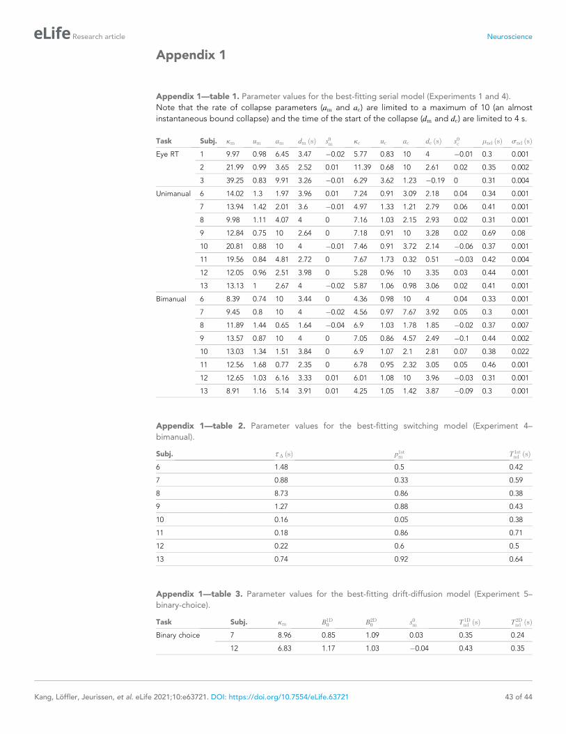
Appendix 1

Appendix 1—table 1. Parameter values for the best-fitting serial model (Experiments 1 and 4).

Note that the rate of collapse parameters (am and ac) are limited to a maximum of 10 (an almost

instantaneous bound collapse) and the time of the start of the collapse (dm and dc) are limited to 4 s.

Task Subj. km um am dm ðsÞ s0m kc uc ac dc ðsÞ s0c �nd ðsÞ snd ðsÞEye RT 1 9.97 0.98 6.45 3.47 �0.02 5.77 0.83 10 4 �0.01 0.3 0.001

2 21.99 0.99 3.65 2.52 0.01 11.39 0.68 10 2.61 0.02 0.35 0.002

3 39.25 0.83 9.91 3.26 �0.01 6.29 3.62 1.23 �0.19 0 0.31 0.004

Unimanual 6 14.02 1.3 1.97 3.96 0.01 7.24 0.91 3.09 2.18 0.04 0.34 0.001

7 13.94 1.42 2.01 3.6 �0.01 4.97 1.33 1.21 2.79 0.06 0.41 0.001

8 9.98 1.11 4.07 4 0 7.16 1.03 2.15 2.93 0.02 0.31 0.001

9 12.84 0.75 10 2.64 0 7.18 0.91 10 3.28 0.02 0.69 0.08

10 20.81 0.88 10 4 �0.01 7.46 0.91 3.72 2.14 �0.06 0.37 0.001

11 19.56 0.84 4.81 2.72 0 7.67 1.73 0.32 0.51 �0.03 0.42 0.004

12 12.05 0.96 2.51 3.98 0 5.28 0.96 10 3.35 0.03 0.44 0.001

13 13.13 1 2.67 4 �0.02 5.87 1.06 0.98 3.06 0.02 0.41 0.001

Bimanual 6 8.39 0.74 10 3.44 0 4.36 0.98 10 4 0.04 0.33 0.001

7 9.45 0.8 10 4 �0.02 4.56 0.97 7.67 3.92 0.05 0.3 0.001

8 11.89 1.44 0.65 1.64 �0.04 6.9 1.03 1.78 1.85 �0.02 0.37 0.007

9 13.57 0.87 10 4 0 7.05 0.86 4.57 2.49 �0.1 0.44 0.002

10 13.03 1.34 1.51 3.84 0 6.9 1.07 2.1 2.81 0.07 0.38 0.022

11 12.56 1.68 0.77 2.35 0 6.78 0.95 2.32 3.05 0.05 0.46 0.001

12 12.65 1.03 6.16 3.33 0.01 6.01 1.08 10 3.96 �0.03 0.31 0.001

13 8.91 1.16 5.14 3.91 0.01 4.25 1.05 1.42 3.87 �0.09 0.3 0.001

Appendix 1—table 2. Parameter values for the best-fitting switching model (Experiment 4–

bimanual).

Subj. t D ðsÞ p1stm T1stnd ðsÞ

6 1.48 0.5 0.42

7 0.88 0.33 0.59

8 8.73 0.86 0.38

9 1.27 0.88 0.43

10 0.16 0.05 0.38

11 0.18 0.86 0.71

12 0.22 0.6 0.5

13 0.74 0.92 0.64

Appendix 1—table 3. Parameter values for the best-fitting drift-diffusion model (Experiment 5–

binary-choice).

Task Subj. km B1D0

B2D0

s0m T1Dnd ðsÞ T2D

nd ðsÞBinary choice 7 8.96 0.85 1.09 0.03 0.35 0.24

12 6.83 1.17 1.03 �0.04 0.43 0.35




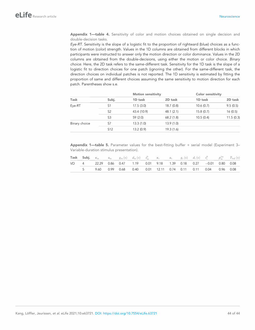
Appendix 1—table 4. Sensitivity of color and motion choices obtained on single decision and

double-decision tasks.

Eye-RT. Sensitivity is the slope of a logistic fit to the proportion of rightward (blue) choices as a func-

tion of motion (color) strength. Values in the 1D columns are obtained from different blocks in which

participants were instructed to answer only the motion direction or color dominance. Values in the 2D

columns are obtained from the double-decisions, using either the motion or color choice. Binary

choice. Here, the 2D task refers to the same-different task. Sensitivity for the 1D task is the slope of a

logistic fit to direction choices for one patch (ignoring the other). For the same-different task, the

direction choices on individual patches is not reported. The 1D sensitivity is estimated by fitting the

proportion of same and different choices assuming the same sensitivity to motion direction for each

patch. Parentheses show s.e.

Motion sensitivity Color sensitivity

Task Subj. 1D task 2D task 1D task 2D task

Eye-RT S1 17.5 (3.0) 18.7 (0.8) 10.6 (0.7) 9.5 (0.5)

S2 43.4 (10.9) 48.1 (2.1) 15.8 (0.7) 16 (0.5)

S3 59 (2.0) 68.2 (1.8) 10.5 (0.4) 11.5 (0.3)

Binary choice S7 13.3 (1.0) 13.9 (1.0)

S12 13.2 (0.9) 19.3 (1.6)

Appendix 1—table 5. Parameter values for the best-fitting buffer + serial model (Experiment 3–

Variable-duration stimulus presentation).

Task Subj. km um gm ðsÞ dm ðsÞ s0m kc uc gc ðsÞ dc ðsÞ s0c p1stm Tbuf ðsÞVD 4 22.29 0.86 0.47 1.19 0.01 9.18 1.39 0.18 0.27 �0.01 0.80 0.08

5 9.60 0.99 0.68 0.40 0.01 12.11 0.74 0.11 0.11 0.04 0.96 0.08




Multiple decisions about one object involve parallel sensory ...

Documents

Transcript of Multiple decisions about one object involve parallel sensory ...