Multiperiod competitive supply chain networks with inventorying and a transportation network...

Multiperiod Competitive Supply Chain Networks with Inventorying and A Transportation Network Equilibrium Reformulation

Multiperiod Competitive Supply Chain Networkswith Inventorying and A Transportation Network

Equilibrium Reformulation

Zugang Liu‡ and Anna Nagurney§

‡Isenberg School of ManagementUniversity of Massachusetts at Amherst

§John F. Smith Memorial ProfessorIsenberg School of Management

University of Massachusetts at Amherst

The Eighteenth Annual Conference of POMSDallas, TX, May 4-7, 2007


Support

Support for this research has been provided by the NationalScience Foundation under Grant No.: IIS-0002647 underDecentralized Decision-Making in Complex Network Systems

This support is gratefully acknowledged


Outline

Outline

Introduction

The related literature

Multiperiod competitive supply chain networks

Transportation network reformulation of the multiperiodcompetitive supply chain network

Numerical examples


Introduction

Dynamic Supply Chains

A supply chain is a network of manufacturers, storage facilitymanagers, transporters and retailers that perform thefunctions of production, storage, transportation, and sale of aparticular product (cf. Nagurney (2006b), Ganeshan andHarrison (1995), Lee and Billington (1995), andSwaminathan, Sadeh, and Smith (1995))

The fundamental function of a supply chain is to matchsupply with demand at the lowest cost (cf. Cachon andTerwiesch (2005))

Highly dynamic and competitive business environments

Fluctuating costs and demands


Introduction

Varying Costs

In the past three years, iron andsteel prices increased by 47%

The price of industrial chemicalsincreased by 51%

Prices of natural gas and crudepetroleum increased by 68%, and112%, respectively

Truck freight transportation costincreased by 6% annually

Water freight transportation costincreased by only 2% annually(source: Bureau of Labor Statistics(2007))


Introduction

Fluctuating Demands

Seasonal fluctuations

E.g. The US automobile market:sales in summer 25− 35% higherthan that in winter

E.g. Many products such as TV,sporting goods and electronicssoar by more than 100% duringthe holiday season (sources: U.S.Census Bureau (2007))


Some of the Related Literature


Decentralized decision-making and competition

Lederer and Li (1997), Cachon and Zipkin (1999), Cachon andNetessine (2003), Geunes and Pardalos (2003), etc.

Dynamic production, inventory, and pricing models

Hafsi and Bai (1998), Federgruen and Tzur (1991), Stadtler(2000), Goyal and Giri (2001), Teng et al. (2002), Perakis andSood (2003, 2006), and Bernstein and Federgruen (2003), etc.

Multiperiod spatial pricing models

Nagurney and Aronson (1988, 1989)




Nagurney, A., Dong, J., Zhang, D., 2002. A Supply ChainNetwork Equilibrium Model. Transportation Research E 38,281-303

Nagurney, A., 2006. On the Relationship Between SupplyChain and Transportation Network Equilibria: A SupernetworkEquivalence with Computations. Transportation Research E42, 293-316




Nagurney, A., Liu, Z., Cojocaru, M., Daniele, P., 2006.Dynamic Electric Power Supply Chains and TransportationNetworks: An Evolutionary Variational Inequality Formulation.Transportation Research E, in press

Wu, K., Nagurney, A., Liu, Z., Stranlund, J., 2006. ModelingGenerator Power Plant Portfolios and Pollution Taxes inElectric Power Supply Chain Networks: A TransportationNetwork Equilibrium Transformation. Transportation ResearchD 11, 171-190

Liu, Z., Nagurney, A., 2006. Financial Networks withIntermediation and Transportation Network Equilibria: ASupernetwork Equivalence and Reinterpretation of theEquilibrium Conditions with Computations. ComputationalManagement Science, in press


Multiperiod Competitive Supply Chain Networks with Inventorying

Multiperiod Supply Chain Networks with Inventorying

Focuses on the supply chain planning process

Captures the changing costs and demands

Provides a flexible platform so that perishable products andtransportation delays can be easily incorporated

The transportation network reformulation provides noveltheoretical insights and efficient computational methods forthe multiperiod supply chain network equilibrium model



The Network Structure of the Multiperiod Supply Chain

jjj

jjj

jjj

?

?

@@@R

@@@R

PPPPPPPq

PPPPPPPq

?

?

HHHHHj

HHHHHj

��

��

?

?

��

��

��)

��)

· · ·

· · ·

· · ·

1, 1

1, 1

1, 1

o, 1k, 1 · · ·

n, 1j, 1 · · ·

m, 1i, 1 · · ·

1

jjj

jjj

jjj

?

?

@@@R

@@@R

PPPPPPPq

PPPPPPPq

?

?

HHHHHj

HHHHHj

��

��

?

?

��

��

��)

��)

· · ·

· · ·

· · ·

1, 2

1, 2

1, 2

o, 2k, 2· · ·

n, 2j, 2· · ·

m, 2i, 2· · ·

2

· · ·

· · ·

· · · jjj

jjj

jjj

?

?

@@@R

@@@R

PPPPPPPq

PPPPPPPq

?

?

HHHHHj

HHHHHj

��

��

?

?

��

��

��)

��)

· · ·

· · ·

· · ·

1, T

1, T

1, T

o, Tk, T· · ·

n, Tj, T· · ·

m, Ti, T· · ·

· · · T

Retailers

Demand Markets

Time Periods

Manufacturers



Manufacturer’s Maximization Problem

MaxTX

t=1

nXj=1

ρ∗1ijtqijt −TX

t=1

fit(qt)−TX

t=1

cvit(uit)−TX

t=1

nXj=1

cijt(qijt)

subject tonX

j=1

qij1 + ui1 = qi1,

uit +nX

j=1

qijt = qit + ui(t−1), t = 2, . . . , T − 1,

nXj=1

qijT = qiT + ui(T−1),

qijt ≥ 0, j = 1, . . . , n; t = 1, . . . , T ,

qit ≥ 0, t = 1, . . . , T ,

uit ≥ 0, t = 1, . . . , T − 1



We assume that the cost functions of the manufacturers areconvex and continuously differentiable and that themanufacturers compete with one another in a noncooperativemanner

The Optimal Conditions for All Manufacturers

Determine:(q∗, u1∗, Q1∗) ∈ K1 satisfying:

TXt=1

mXi=1

∂fit(q∗t )

∂qit× [qit − q∗it ] +

TXt=1

mXi=1

nXj=1

�∂cijt(q

∗ijt)

∂qijt− ρ∗1ijt

�×�qijt − q∗ijt

�

+TX

t=1

mXi=1

∂cvit(u∗it)

∂uit× [uit − u∗it ] ≥ 0, ∀(q, u1, Q1) ∈ K1,

where K1 ≡ {(q, u1, Q1)|(q, u1, Q1) ∈R

Tm(2+n)+ and the conservation of flow equations hold}



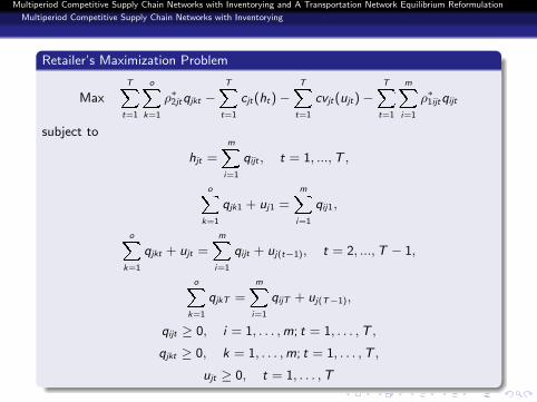
Retailer’s Maximization Problem

MaxTX

t=1

oXk=1

ρ∗2jtqjkt −TX

t=1

cjt(ht)−TX

t=1

cvjt(ujt)−TX

t=1

mXi=1

ρ∗1ijtqijt

subject to

hjt =mX

i=1

qijt , t = 1, ..., T ,

oXk=1

qjk1 + uj1 =mX

i=1

qij1,

oXk=1

qjkt + ujt =mX

i=1

qijt + uj(t−1), t = 2, ..., T − 1,

oXk=1

qjkT =mX

i=1

qijT + uj(T−1),

qijt ≥ 0, i = 1, . . . , m; t = 1, . . . , T ,

qjkt ≥ 0, k = 1, . . . , m; t = 1, . . . , T ,

ujt ≥ 0, t = 1, . . . , T



We assume that the cost functions of the retailers are convexand continuously differentiable and that the retailers competewith one another in a noncooperative manner

The Optimal Conditions for All Retailers

determine (Q1∗, h∗, u2∗, Q2∗) ∈ K2 satisfying:

TXt=1

nXj=1

∂cjt(h∗t )

∂hjt×�hjt − h∗jt

�

+TX

t=1

mXi=1

nXj=1

ρ∗1ijt ×�qijt − q∗ijt

�−

TXt=1

nXj=1

oXk=1

ρ∗2jt ×�qjkt − q∗jkt

�

+TX

t=1

nXj=1

∂cvjt(u∗jt)

∂ujt×�ujt − u∗jt

�≥ 0, ∀(Q1, h, u2, Q2) ∈ K2,

where K2 ≡ {(Q1, h, u2, Q1)|(Q1, h, u2, Q1) ∈R

Tn(m+o+2)+ and the conservation of flow equations hold}



The Equilibrium Conditions for Consumers at the Demand Markets

The equilibrium conditions for consumers at demand market k, take the form:for all retailers j ; j = 1, . . . , n and time periods t; t = 1, . . . , T :

ρ∗2jt + cjkt(Q2t∗)

�= ρ∗3kt , if q∗jkt > 0,≥ ρ∗3kt , if q∗jkt = 0,

and

dkt(ρ∗3t)

8>>>><>>>>:

=nX

j=1

q∗jkt , if ρ∗3kt > 0,

≤nX

j=1

q∗jkt , if ρ∗3kt = 0



Equilibrium Conditions of the Multiperiod Supply ChainNetwork

Definition: Multiperiod Supply Chain Network Equilibrium

The equilibrium state of the multiperiod supply chain network isone where the flows of the product between the tiers of thedecision-makers coincide and the flows and prices satisfy the sumof the optimality conditions and equilibrium conditions so that nodecision-maker has any incentive to alter his transactions.



Theorem: Variational Inequality Formulation of the Multiperiod SupplyChain Network Equilibrium

Determine: (q∗, h∗, u1∗, Q1∗, u2∗, Q2∗, d∗, ρ∗3 ) ∈ K3 satisfying:

TXt=1

mXi=1

∂fit(q∗t )

∂qit× [qit − q∗it ] +

TXt=1

mXi=1

nXj=1

∂cijt(q∗ijt)

∂qijt×�qijt − q∗ijt

�

+TX

t=1

nXj=1

∂cjt(h∗t )

∂hjt×�hjt − h∗jt

�+

TXt=1

mXi=1

∂cvit(u∗it)

∂uit× [uit − u∗it ]

+TX

t=1

nXj=1

∂cvjt(u∗jt)

∂ujt×�ujt − u∗jt

�+

TXt=1

nXj=1

oXk=1

cjkt(Q2∗t )×

�qjkt − q∗jkt

�

+TX

t=1

oXk=1

ρ∗3kt × [dkt − d∗kt ] +TX

t=1

oXk=1

[d∗kt − dkt(ρ∗3t)]× [ρ3kt − ρ∗3kt ] ≥ 0,

∀(q, h, u1, Q1, u2, Q2, d , ρ3) ∈ K3,

where K3 ≡ {(q, h, u1, Q1, u2, Q2, d , ρ3)|(q, h, u1, Q1, u2, Q2, d , ρ3) ∈R

T (2m+mn+2n+no+2o)+ and the conservation of flow equations hold}


Transportation Network Equilibrium Model with Known Demand Functions

Transportation Network Equilibrium Model with KnownDemand Functions (Dafermos and Nagurney (1984))

Define the set of origin/destination (O/D) pairs W with Zelements; the set of paths P with Q elements; the set of linksL with K elementsThe conservation of flow equations must hold:

dw =∑p∈Pw

xp, ∀w ∈ W

fa =∑p∈P

xpδap, ∀a ∈ L

The user cost on a path is equal to the sum of user costs onlinks the path consists of

Cp =∑a∈L

caδap, ∀p ∈ P


Transportation Network Equilibrium Model with Known Demand Functions

Transportation Network Equilibrium Model with KnownDemand Functions

TheoremA travel link flow pattern and associated travel demand anddisutility pattern is a transportation network equilibrium if and onlyif it satisfies the variational inequality problem: determine(f ∗, d∗, λ∗) ∈ K4 satisfying∑

a∈L

ca(f∗)× (fa − f ∗a )−

∑w∈W

λ∗w × (dw − d∗

w )

+∑

w∈W

[d∗w − dw (λ∗)]× [λw − λ∗

w ] ≥ 0, ∀(f , d , λ) ∈ K4,

where K4 ≡ {(f , d , λ) ∈ RK+2Z+ |

there exists an x satisfying the conservation of flow equations}


Transportation Network Equilibrium Reformulation of the Multiperiod Supply Chain Network

The GS Supernetwork Representation of theMultiperiod Supply Chain Network

j0

jjjj

jjjj

jjjj

?

?

?

@@@R

@@@R

PPPPPPPq

PPPPPPPq

?

?

?

HHHHHj

HHHHHj

��

��

?

?

?

��

��

��)

��)

· · ·

· · ·

· · ·

· · ·

z11 zz1zk1 · · ·

y1′1 yn′1yj′1 · · ·

y11 yn1yj1 · · ·

x11 xm1xi1 · · ·

am2

amn2

ann′2

an′o2

am2(3)

an′2(3)

jjjj

jjjj

jjjj

?

?

?

@@@R

@@@R

PPPPPPPq

PPPPPPPq

?

?

?

HHHHHj

HHHHHj

��

��

?

?

?

��

��

��)

��)

· · ·

· · ·

· · ·

· · ·

z12 zk2 zo2· · ·

y1′2 yn′2yj′2 · · ·

y12 yn2yj2 · · ·

x12 xm2xi2 · · ·

· · ·

· · ·

· · · jjjj

jjjj

jjjj

?

?

?

@@@R

@@@R

PPPPPPPq

PPPPPPPq

?

?

?

HHHHHj

HHHHHj

��

��

?

?

?

��

��

��)

��)

· · ·

· · ·

· · ·

· · ·

z1T zkT zoT· · ·

y1′T yn′Tyj′T · · ·

y1T ynTyjT · · ·

x1T xmTxiT · · ·



Transportation Network Equilibrium Reformulation ofthe Multiperiod Supply Chain Network

New interpretation of the supply chain network equilibrium interms of paths and path flows

Competition among end-to-end supply chains

Efficient computational method



The Euler Method

Let T denote an iteration counter

Step 0: InitializationSet X 0 ∈ KLet T = 1 and set the sequence {αT } so that

P∞T =1 αT = ∞, αT > 0 for all

T , and αT → 0 as T → ∞Step 1: ComputationCompute XT ∈ K by solving the variational inequality subproblem:

〈XT + αT F (XT −1)− XT −1, X − XT 〉 ≥ 0, ∀X ∈ K

Step 2: Convergence VerificationIf |XT −XT −1| ≤ ε, with ε > 0, a pre-specified tolerance, then stop; otherwise,set T := T + 1, and go to Step 1


Numerical Examples

Numerical Examples 1 and 2

Example 1 has 2 manufacturers, 2 retailers, 2 demand marketsand 3 periods

Example 2 has the same data as Example 1 except that theproduct in Example 2 is perishable (L = 2)


Numerical Examples

The Network Structure of Numerical Examples 1 and 2

mmm

mmm

?

?

@@

@R

@@

@R

?

?

��

�

��

�

1, 1

1, 1

1, 1

2, 1

2, 1

2, 1

1

mmm

mmm

?

?

@@

@R

@@

@R

?

?

��

�

��

�

1, 2

1, 2

1, 2

2, 2

2, 2

2, 2

Time Periods

2

mmm

mmm

?

?

@@

@R

@@

@R

?

?

��

�

��

�

1, 3

1, 3

1, 3

2, 3

2, 3

2, 3

3

Retailers

Demand Markets

Manufacturers


Numerical Examples

Supernetwork Structure of the Transportation NetworkEquilibrium Reformulation of Examples 1 and 2l0

llll

llll

?

?

?

@@@R

@@@R

?

?

?

��

�

��

�

z11z21

y1′1y2′1

y11y21

x11x21

llll

llll

?

?

?

@@@R

@@@R

?

?

?

��

�

��

�

z12 z22

y1′2 y2′2

y12 y22

x12 x22

llll

llll

?

?

?

@@@R

@@@R

?

?

?

��

�

��

�

z13 z23

y1′3 y2′3

y13 y23

x13 x23


Numerical Examples

Cost Functions of Examples 1 and 2

The production cost functions:

f1t(q1t) = 0.1q21t +5q1t +20, f2t(q2t) = 0.15q2

2t +4q2t +10, t = 1, 2, 3

The transaction/transportation cost functions:

c11t(q11t) = 0.005q211t + q11t , c12t(q12t) = 0.005q2

12t + q12t ,

c21t(q21t) = 0.005q221t + q21t , c22t(q22t) = 0.005q2

22t + q22t , t = 1, 2, 3

The handling costs of the retailers:

c1t(h1t) = 0.05h21t +1.5h1t +20, c2t(h2t) = 0.1h2

2t +h2t +30, t = 1, 2, 3


Numerical Examples

Cost Functions of Examples 1 and 2 (Cont’)

The inventory cost functions of the manufacturers:

cv1t(u1t) = 0.025u21t+0.5u1t+10, cv2t(u2t) = 0.025u2

2t+0.5u2t+20, t = 1, 2

The inventory costs functions of the retailers:

cv1t(u1t) = 0.025u21t + 0.5u1t , cv2t(u2t) = 0.025u2

2t + 0.5u2t , t = 1, 2

The demand functions:

d11(ρ311) = 15−1

2ρ311, d12(ρ312) = 20−1

3ρ312, d13(ρ313) = 80− 1

10ρ313,

d21(ρ321) = 10− 1

2ρ321, d22(ρ322) = 15− 1

3ρ322, d23(ρ323) = 90− 1

10ρ323


Numerical Examples

Equilibrium Solutions of Examples 1 and 2

Example 1 Example 2Variable t = 1 t = 2 t = 3 t = 1 t = 2 t = 3f ∗a1t

= q∗1t 32.6997 36.3997 40.5709 18.5877 45.5601 49.1646

f ∗a2t= q∗2t 25.2589 27.7443 30.5455 15.7721 33.9027 36.3221

f ∗a11t= q∗11t 16.6645 21.3144 29.6492 11.2588 24.2616 33.5997

f ∗a12t= q∗12t 11.2351 13.2002 17.6067 7.3289 16.8807 19.9826

f ∗a21t= q∗21t 12.8955 16.9915 24.6881 9.8501 18.3844 27.2268

f ∗a22t= q∗22t 7.4509 8.8588 12.6637 5.9219 11.0021 13.6114

f ∗a11′t

= h∗1t 29.5601 38.3060 54.3373 21.1089 42.6460 60.8265

f ∗a22′t

= h∗2t 18.6860 22.0591 30.2705 13.2509 27.8829 33.5940

f ∗a1′1t

= q∗11t 5.4186 12.8893 38.7451 6.4787 5.2527 46.0004

f ∗a1′2t

= q∗12t 0.9186 8.2277 56.0039 2.4797 6.8976 57.4722

f ∗a2′1t

= q∗21t 0.0000 0.1694 38.9204 0.8006 9.2310 31.4244

f ∗a2′2t

= q∗22t 0.0000 0.1643 31.7615 0.2996 2.9194 30.0525

f ∗a1t(t+1)= u∗1t 4.8001 6.6850 0.0000 0.0000 4.4177 0.0000

f ∗a2t(t+1)= u2t 4.9124 6.8063 0.0000 0.0000 4.5162 0.0000

f ∗a1′t(t+1)

= u∗1t 23.2227 40.4117 0.0000 12.1504 42.6460 0.0000

f ∗a2′t(t+1)

= u∗2t 18.6860 40.4114 0.0000 12.1505 27.8829 0.0000

d∗w1t = d∗1t 5.4186 13.0587 77.6655 7.2794 14.4838 77.4248

d∗w2t = d∗2t 0.9186 8.3920 87.7655 2.7794 9.8171 87.5248

λ∗w1t = ρ∗31t 19.1626 20.8237 23.3443 15.4410 16.5485 25.7515

λ∗w2t = ρ∗32t 18.1626 19.8237 22.3443 14.4410 15.5485 24.7515


Numerical Examples

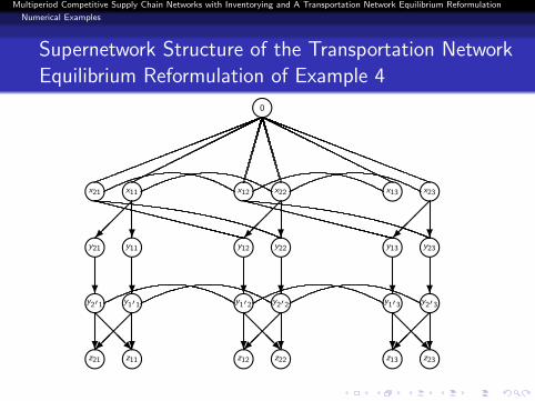
Numerical Examples 3 and 4

Examples 3 and 4 have inseparable cost functions

Example 3 has the same network structure as Examples 1 and2

In Example 4, manufacturer 1 has one-period transportationdelay


Numerical Examples

The Network Structure of Example 4 (TransportationDelay)

mmm

mmm

?

@@

@R?

?

��

�

��

�

1, 1

1, 1

1, 1

2, 1

2, 1

2, 1

1

mmm

mmm

?

@@

@R?

?

��

�

��

�

1, 2

1, 2

1, 2

2, 2

2, 2

2, 2

Time Periods

2

mmm

mmm

?

@@

@R?

?

��

�

��

�

1, 3

1, 3

1, 3

2, 3

2, 3

2, 3

3

Retailers

Demand Markets

Manufacturers


Numerical Examples

Supernetwork Structure of the Transportation NetworkEquilibrium Reformulation of Example 4l0

llll

llll

?

?

@@@R?

?

?

��

�

��

�

z11z21

y1′1y2′1

y11y21

x11x21

llll

llll

?

?

@@@R?

?

?

��

�

��

�

z12 z22

y1′2 y2′2

y12 y22

x12 x22

llll

llll

?

?

@@@R?

?

?

��

�

��

�

z13 z23

y1′3 y2′3

y13 y23

x13 x23


Numerical Examples

Cost Functions of Examples 3 and 4

The production cost functions:

f1t(q1t , q2t) = 5 + q1t + 0.4q21t + 0.2q1tq2t , t = 1, 2, 3,

f2t(q1t , q2t) = 10 + 2q2t + 1.5q22t + 0.4q1tq2t , t = 1, 2, 3

The transaction/transportation cost functions:

c11t(q11t) = 3q11t + 0.1q211t , c12t(q12t) = 3q12t + 0.1q2

12t ,

c21t(q21t) = q21t + 0.1q221t , c22t(q22t) = q22t + 0.1q2

22t , t = 1, 2, 3

The handling costs of the retailers:

c1t(h1t , h2t) = 0.1h21t+0.1h1th2t , t = 1, 2, 3, c2t(h1t , h2t) = 0.1h2

2t+0.1h1th2t , t = 1, 2, 3.


Numerical Examples

Cost Functions of Examples 3 and 4 (Cont’)

The inventory cost functions of the manufacturers:

cv1t(u1t) = 0.2u21t + u1t , t = 1, 2, cv2t(u2t) = 0.5u2

2t + 2u2t , t = 1, 2

The inventory costs functions of the retailers:

cv1t(u1t) = 0.05u21t+u1t , t = 1, 2, cv2t(u2t) = 0.02u2

2t+u2t , t = 1, 2.

The demand functions:

d11(ρ311) = 70− ρ311, d12(ρ312) = 80− ρ312, d13(ρ313) = 90− ρ313,

d21(ρ321) = 55−0.2ρ321, d22(ρ322) = 55−0.2ρ322, d23(ρ323) = 60−0.2ρ323


Numerical Examples

Equilibrium Solutions of Examples 3 and 4

Example 3 Example 4Variable t = 1 t = 2 t = 3 t = 1 t = 2 t = 3f ∗a1t

= q∗1t 50.8291 51.9564 53.1257 49.4331 53.4121 0.0000

f ∗a2t= q∗2t 9.1084 9.3028 9.5044 30.4517 9.7468 16.4581

f ∗a11t= q∗11t 25.4145 25.9782 26.5628 24.7165 26.7060 0.0000

f ∗a12t= q∗12t 25.4145 25.9782 26.5628 24.7165 26.7060 0.0000

f ∗a21t= q∗21t 4.5542 4.6514 4.7522 15.2258 4.8734 8.2290

f ∗a22t= q∗22t 4.5542 4.6514 4.7522 15.2258 4.8734 8.2290

f ∗a11′t

= h∗1t 29.9688 30.6296 31.3150 15.2258 29.5900 34.9351

f ∗a22′t

= h∗2t 29.9688 30.6296 31.3150 15.2258 29.5900 34.9351

f ∗a1′1t

= q∗11t 2.3862 6.3799 14.7593 0.0000 7.6204 12.3561

f ∗a1′2t

= q∗12t 21.2911 23.0842 24.0125 15.2258 20.8777 23.6708

f ∗a2′1t

= q∗21t 6.0551 10.8097 11.1321 0.0000 7.9223 12.1430

f ∗a2′2t

= q∗22t 21.3970 19.3536 23.1657 15.2258 21.2307 23.2289

f ∗a1t(t+1)= u∗1t 0.0000 0.0000 0.0000 0.0000 0.0000 0.0000

f ∗a2t(t+1)= u∗2t 0.0000 0.0000 0.0000 0.0000 0.0000 0.0000

f ∗a1′t(t+1)

= u∗1t 6.2914 7.4568 0.0000 0.0000 1.0917 0.0000

f ∗a2′t(t+1)

= u∗2t 2.5165 2.9827 0.0000 0.0000 0.4368 0.0000

d∗w1t = d∗1t 8.4413 17.1897 25.8914 0.0000 15.5428 24.4991

d∗w2t = d∗2t 42.6882 42.4379 46.3314 30.4517 42.1085 46.8998

λ∗w1t = ρ∗31t 61.5586 62.8102 64.1085 70.0000 64.4571 65.5008

λ∗w2t = ρ∗32t 61.5586 62.8102 64.1085 122.7413 64.4571 65.5008


Conclusions

Conclusions

Developed the multiperiod competitive supply chain networkmodel with varying costs and demands

Established the supernetwork equivalence betweentransportation networks and multiperiod competitive supplychain networks

The model provides a flexible platform so that perishableproducts and transportation delays can be easily incorporated

The transportation network reformulation provides noveltheoretical insights and efficient computational methods forthe multiperiod supply chain network equilibrium model


Conclusions

Thank You!

For more information, please see:The Virtual Center for Supernetworks

http://supernet.som.umass.edu

Multiperiod competitive supply chain networks with inventorying and a transportation network...

Documents

Transcript of Multiperiod competitive supply chain networks with inventorying and a transportation network...