Multilevel address reorganization type2 in wireless personal area network

International Journal of Wireless & Mobile Networks (IJWMN) Vol. 5, No. 1, February 2013

DOI : 10.5121/ijwmn.2013.5104 47

MULTILEVEL ADDRESS REORGANIZATION TYPE2

IN WIRELESS PERSONAL AREA NETWORK

Debabrato Giri1 and Uttam Kumar Roy

2

1Department of Information Technology, Jadavpur University, Kolkata, India

[email protected] 2 Department of Information Technology, Jadavpur University, Kolkata, India

[email protected]

ABSTRACT

The Standard for Wireless personal area network (WPAN) has been given by IEEE 802.15.4-2003 these

networks are consists of Low rate, Low powered, Low memory devices. ZigBee Alliance has provided

Network layer specification and Physical layer (PHY) and Medium access control (MAC) specification

has been given by IEEE. In general the networks are of two kind Tree/Mess. In tree network no routing

table is required for routing. After the great success in PAN this technique has also been tried to apply in

business Network too. The main problem with this routing is that the maximum no of child (Router

capable or end device) at any level and maximum network depth is fixed and this is done at the time of

network formation. So the network can’t grow beyond that max limit of breadth and width. We have

addressed the network depth problem in our paper “Address Borrowing in Wireless Personal Area

Network”. Now in some other network configuration the maximum breadth of the network may be

attained but the maximum depth of the network may not be attained (because of the asymmetric nature of

the physical area) at that part and hence address lies unused. Here In this paper we have provided a

unified address reorganizing scheme which can be easily applied to tree network so that the network can

grow beyond the maximum no of child present at any level and overcome the address exhaustion problem

by reorganizing address as per the requirement but without adding any extra overhead of having a

routing table.

KEYWORDS

PAN; Mesh; Address Reorganizing; Routing; WPAN; Tree;

1. INTRODUCTION

In recent past there has been a steady rise in wireless networking. Wireless sensor/actuator

networks (“sensornets”) represents a new computing class consisting of large number of nodes

which are often embedded in their operating environments distributed over wide geographical

area often in remote and largely inaccessible regions. The node themselves ranges from tiny ,

resource-constrained devices called motes to PDA-class computing devices that are capable of

sensing, computation, communication , and actuation. Sensornets allows us to instrument,

observe, and respond to the physical world on scales of space and time previously impossible.

Standards like IEEE 802.11[11] (Wi-Fi) and IEEE 802.15.1 [13] (12) have come into existence.

IEEE 802.11 targets high data rate, mains powered, high cost and relatively long range

applications. Bluetooth is one of the first standards designed for low range, low power devices.

Because of its huge popularity now a day all most all the mobiles are coming with Bluetooth.

But the main problem with this technology is the data can be transferred to single hop only. As a

result more and more low-cost high-quality devices appear in the market; short-range low-rate

wireless personal area networks are poised to take the world in a way observed never before

which can transfer the data using multiple hops.


48

Wireless personal area networks (WPANs) are used to convey information over relatively short

distances. Unlike wireless local area networks (WLANs), connections effected via WPANs

involve little or no infrastructure. This feature allows small, power-efficient, inexpensive

solutions to be implemented for a wide range of devices.

IEEE 802.15.4 [19] (henceforth referred to as 802.15.4) is a landmark in the attempt to bring

ubiquitous networking [Figure 1] into our lives. Designed uniquely for energy-conscious low

data rate appliances, it specifies the PHYsical (PHY) layer and MAC sub-layer of the protocol

stack. The ZigBee Alliance [19] has defined the specification for the network (NWK), security

and application profile layers for an 802.15.4-based system. Network layer supports three

topologies Star, Tree and Mesh. The main advantage of tree address allocation is that it does not

require any routing table to forward a message. In that simple mathematical equations are used

for address assignment and routing.

With ZigBee devices on the horizon, ubiquitous networking looks elusive no more. It is not too

distant a future one may chance to have one’s home-appliances wedded together in a smart and

cooperative network that allows them to talk to each other seamlessly. Sensors and actuators

will communicate without barrier. They can be deployed pervasively in disaster-hit areas to

monitor the situation to provide situational awareness and automatically take appropriate

actions.

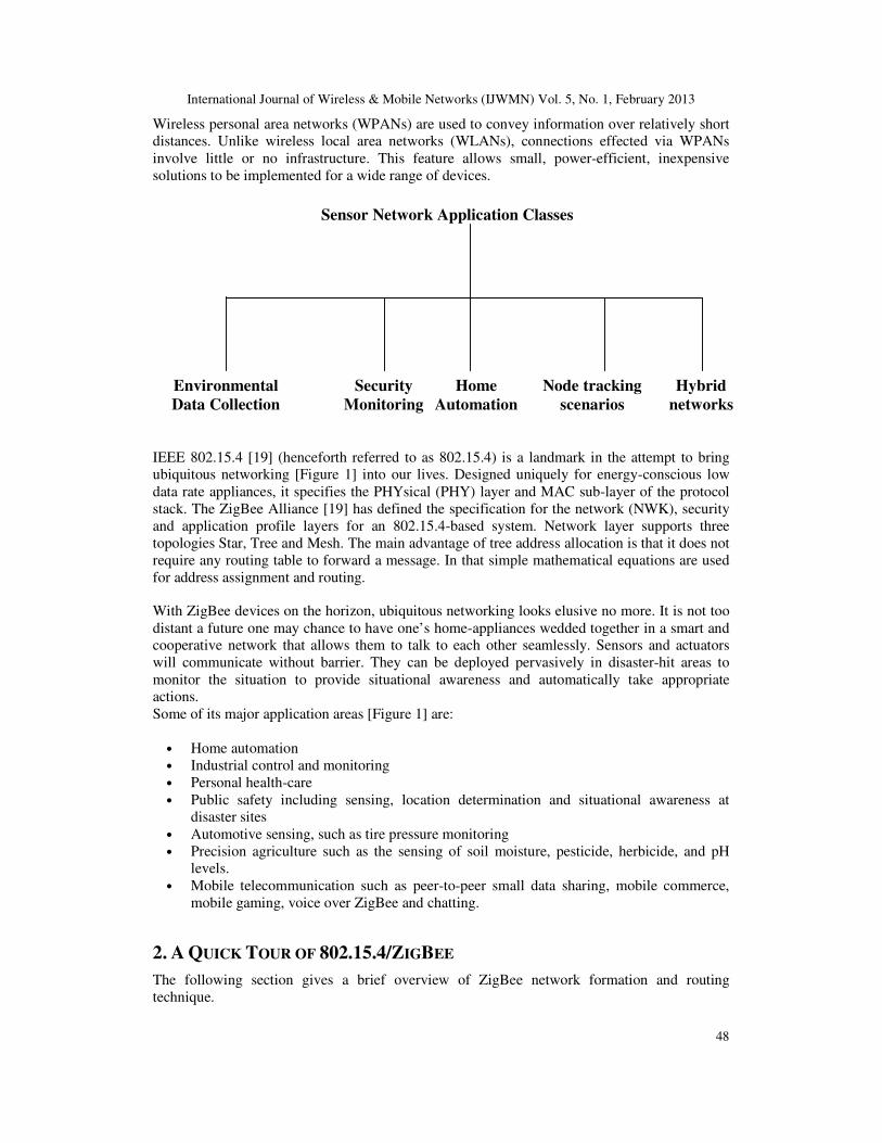
Some of its major application areas [Figure 1] are:

• Home automation

• Industrial control and monitoring

• Personal health-care

• Public safety including sensing, location determination and situational awareness at

disaster sites

• Automotive sensing, such as tire pressure monitoring

• Precision agriculture such as the sensing of soil moisture, pesticide, herbicide, and pH

levels.

• Mobile telecommunication such as peer-to-peer small data sharing, mobile commerce,

mobile gaming, voice over ZigBee and chatting.

2. A QUICK TOUR OF 802.15.4/ZIGBEE

The following section gives a brief overview of ZigBee network formation and routing

technique.

Sensor Network Application Classes

Environmental

Data Collection

Security

Monitoring

Node tracking

scenarios

Hybrid

networks

Home

Automation


49

2.1. 802.15.4/ZigBee target applications

With ZigBee devices on the horizon, ubiquitous networking looks elusive no more. It is not too

distant a future one may chance to have one’s home-appliances wedded together in a smart and

cooperative network that allows them to talk to each other seamlessly. Sensors and actuators

will communicate without barrier. They can be deployed pervasively in disaster-hit areas to

monitor the situation to provide situational awareness and automatically take appropriate

actions.

Some of its major application areas [Figure 1] are:

• Home automation

• Industrial control and monitoring

• Personal health-care

• Public safety including sensing, location determination and situational awareness at

disaster sites

• Automotive sensing, such as tire pressure monitoring

• Precision agriculture such as the sensing of soil moisture, pesticide, herbicide, and pH

levels.

• Mobile telecommunication such as peer-to-peer small data sharing, mobile commerce,

mobile gaming, voice over ZigBee and chatting.

Figure 1: An example of home automation

2.2. Highlights of 802.15.4 standard

This standard is a specification of the PHYsical layer (PHY) and Medium Access Control

(MAC) sub-layer for low data rate wireless connectivity among relatively simple devices that

consume minimal power and typically operate in a Personal Operating Space (POS) of 10

meters or less. The network can be a one-hop star, or, when lines of communication exceed 10

meters, a self-configuring, multi-hop ad-hoc network.

2.3. ZigBee Value Addition

The ZigBee Alliance defines the network (NWK), security, and application profile layers for the

802.15.4-based system. Two routing (Tree and Mesh routing) protocols have been defined. The

algorithms are kept lightweight as devices are expected to be simple and have small memory.


50

Note that traditional table-driven ad hoc wireless routing protocols such as DSDV [2], CGSR,

WRP, AODV [1, 3], require significant amount of memory for maintaining routing tables and

hence are not suitable for these types of devices. Source-initiated routing such DSR [4], LMR,

TORA, ABR, SSR may be considered as alternatives as they do not use any routing table. But,

for a long network, incorporating routing information in the packet y the source is not practical

due to the limitation on maximum packet size (16 bytes). Moreover, data rate is very low (e.g.

not more that 100 packets throughout the day for a personal area network for home appliance)

that requires a relatively light-weight routing algorithm which incurs an overhead as small as

possible.

2.4. ZigBee Device Types

A device in a Zigbee network can be physically a Full Function Device (FFD) or a Reduced

Function Device (RFD). An FFD typically has more resources than an RFD. Logically a

Zigbee-device can be a

•ZigBee coordinator: 802.15.4 PAN coordinator for a ZigBee network—must be an FFD.

•ZigBee router: 802.15.4 FFD that is not the ZigBee coordinator but capable of being so and

participates in mesh routing.

•ZigBee end-device: 802.15.4 RFD or FFD that is not a ZigBee coordinator..

2.5. Topologies Supported by Network Layer.

The ZigBee network (NWK) layer supports star, tree and mesh topologies. In a star topology,

the network is controlled by one single device called ZigBee coordinator. The ZigBee

coordinator is responsible for initiating and maintaining network. All other devices, known as

end devices, directly communicate with the ZigBee coordinator. In mesh and tree topologies,

the ZigBee coordinator is responsible for starting the network and for choosing certain key

network parameters but the network may be extended through the use of ZigBee routers. In tree

networks, routers move data and control messages through the network using a hierarchical

routing strategy. Mesh networks allow full peer- to-peer communication.

2.6. Network Address Assignment

Network addresses are assigned using a distributed addressing scheme that is designed to

provide a finite sub-block of network addresses to every potential parent. These addresses are

unique within a particular network and are given by a parent to its children. The ZigBee

coordinator determines the maximum number of children (nwkMaxChildren) that any device

within its network is allowed. Of these children, a maximum of nwkMaxRouters can be router-

capable devices while the rest will be reserved for end devices. But no hint is given how these

parameters are determined. Every device has an associated depth, which indicates the minimum

number of hops to reach ZigBee coordinator. The ZigBee coordinator itself has a depth of zero,

while its children have a depth of one. Multi-hop networks have a maximum depth that is

greater than one. The ZigBee coordinator also determines the maximum depth (nwkMaxDepth)

of the network.

Given the following network parameters:

Cm = maximum number of children a ZigBee device may accept, nwkMaxChildren

Lm = maximum depth in the network, nwkMaxDepth


51

Rm = maximum number of router-capable-children a ZigBee device may accept,

nwkMaxRouters

Em[=(Cm-Rm)] = maximum number of end-devices a ZigBee device may accept as children

We may compute the function, Cskip(d), essentially the size of the address sub-block distributed

by each parent at depth d to each of its router-capable child devices, as follows:

≠≠

−

−−+

≠=−−+

=

=

−−

m

m

dL

mmmm

mmmm

m

skip

LdRR

RCRC

LdRdLC

Ld

dC

m

,1:1

.1

,1:),1.(1

:0

)(

1

(1)

If a device has a Cskip(d) value of zero, then it shall not be capable of accepting children and

shall be treated as a ZigBee end device. A device that has a Cskip(d) value greater than zero may

accept child devices and may assign addresses to them differently depending on whether the

child device is router-capable or not. Network addresses are assigned to router-capable child

devices using the value of Cskip(d) as an offset.

A router-capable device having address Aparent at depth d assigns addresses to its nth

child An at

depth d+1 in the following way:

END-DEVICE CHILD:

mmskipparentn EnnRdCAA ≤≤++= 1:)( (2)

ROUTER-CAPABLE CHILD:

mskipparentn RnndCAA ≤≤+−+= 1:1)1)(( (3)

The first router-capable child gets address Aparent+1 and subsequent router-capable children get

addresses separated by Cskip(d). End-devices get addresses starting from Aparent+1+Cskip(d)*Rm

separated by 1. Such example is shown in Figure. 3 and Figure 6.

2.7. Tree Routing Mechanism

For hierarchical routing, if the destination is a descendant of the device, the device shall route

the frame to the appropriate child. Trivially, every other device is a descendant of the ZigBee

Coordinator and no device is a descendant of any ZigBee end-device.

Refer to (1), (2) and (3), taking a routing decision is very simple. A target device with address D

is a descendant of a ZigBee router with address A at depth d if

)1( −+<< dCADA skip (4)

This follows because the parent P at depth (d-1) of the device X with address A, gives the

address A to X and the address A+Cskip(d-1) to the “closest” router-capable-sibling of X that is


52

also a child of P. The address sub-block [A+1, A+Cskip(d-1)-1] is reserved for the descendants

of X.

If the destination is a descendant of the receiving device, the address N of the next hop device is

determined as:

×

+−++

×+>

=

otherwisedCdC

ADA

devicesendfordCRADifD

Nskip

skip

skipm

),()(

)1(1

)(,

(5)

If equation (5) is not satisfied, next hop device is its parent. We look below at the derivation of

formula (6):

The next-hop address is N=A+1+kCskip(d), i.e. the packet is to be routed to the router-capable-

child with address A+1+kCskip(d) if A+1+kCskip(d) ≤D< A+1+(k+1)Cskip(d)

This is because the device with address A+1+kCskip(d) gets address sub-block [A+1+kCskip(d),

A+1+(k+1)Cskip(d)-1] i.e. ),(1 dkCAN skip++=

Where

1)(

1+<

−−≤ k

dC

ADk

skip

−−=⇒

)(

1

dC

ADk

skip

(6)

So, next hop router can be determined by using an equation and the complexity of this scheme

is constant. Moreover, there is no routing table and that way searching procedure is completely

eliminated. In spite of this, tree routing has several limitations as described in the next section.

2.8. Problem Definition

The fundamental query that arises regarding tree routing is “how to choose the values of Cm and

Rm?”. In many cases, before actually forming the network, we have very little or no idea about

the following parameters:

o Number of end devices that will join to a router

o Number of routers that will join to a router

o Depth of the tree network

Also once the value is chosen the address distribution will be symmetric and it will not be able

to support asymmetric structures required in mine field, glaciers sea bed, building premises etc.

Because an address sub-block cannot be shared between devices, it is possible that one parent

exhausts its list of addresses while a second parent has addresses that go unused. A parent

having no available addresses shall not permit a new device to join the network. In this

situation, the new device shall find another parent. If no other parent is available within

transmission range of the new device, the device shall be unable to join the network unless it is

physically moved or there is some other change.


53

This routing technique uses a fixed address assignment i.e. the no of child are fixed at any level

and hence the address range, it is possible to have a network in which the no of child per parent

increases as the depth increases, in this kind of network a large range of address will remain

unused at the top level

Finally, due to the fact that the tree, it is not dynamically balanced, the possibility exists that

certain installation scenarios, such as long lines of devices, may exhaust the address capacity of

the network long before the real capacity is reached.

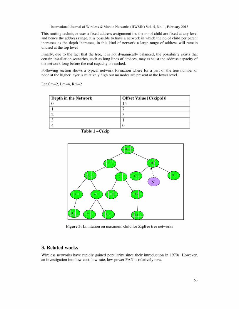
Following section shows a typical network formation where for a part of the tree number of

node at the higher layer is relatively high but no nodes are present at the lower level.

Let Cm=2, Lm=4, Rm=2

Depth in the Network Offset Value [Cskip(d)]

0 15

1 7

2 3

3 1

4 0

Table 1 –Cskip

Figure 3: Limitation on maximum child for ZigBee tree networks

3. Related works

Wireless networks have rapidly gained popularity since their introduction in 1970s. However,

an investigation into low-cost, low-rate, low-power PAN is relatively new.

0

1 16

9 24 17 2

3 6

4 7

13 10

8 14

N


54

In [6], we have provided a unified address borrowing scheme which can be easily applied to

grow the network beyond 16 hops and overcome the address exhaustion problem by borrowing

address. A routing algorithm based on mobile IP, is also proposed.

In [7], we extended the Tree routing proposed by ZigBee for the networks to be harsh and

asymmetric.

4. Proposed Address Reorganization Algorithm

In this paper we have extended our solution of single level address re-organization to multiple

levels with out any extra over head such as routing table. The next hop address is calculated

using mathematical formula only .This algorithm will allow the formation of any asymmetric

network as per the need and thus remove the limitation of symmetric address distribution and

formation. In real world most of the networks area is asymmetric for example in a building the

lower floors can have more rooms compared to upper floors and part of ground floor may have

canteen/gym etc so does not require any network or a paddy field can have some irregular

shape, proposed address reorganization technique is capable of handling all these and can be

applied to all such asymmetric networks.

In this scheme a node will be allowed to join a network at a node even if it has reached

maximum no child by Address reorganization. This scheme can be used in part of the network

where the network wants to grow in breadth rather than in depth i.e. we are expecting that the

depth will be less than Lm at that part of the network. In Figure 3 the maximum length of the

path from root which goes via Node 16 is two i.e. the depth of the network at that part is 2(less

than Lm) which suggests that at that part of the network the growth is around the breadth and

not in depth . We can apply our algorithm at that part.

In proposed address reorganization scheme any parent can increase its no of child device by

reorganizing its address by any level so it is much more flexible.

4.1. Overview of the Algorithm

The Node which has reached its maximum child and wants to expand its breadth will use the

next level Cskip value while distributing the address to its child i.e. if the node is at level K it

will use the Cskip value for K+1, its immediate child will use K+2 and so on till Lm-1.By doing

this the Node has gained one level of address which it can use for adding new child.In Figure 3

if a new node wants to join the network at Node 16 then it will not be allowed as Node 16 has

exhausted its address even though free address is available at other node such as Node 17 or

Node 24.Our proposed algorithm could be used in such scenarios.

After address reorganizing the maximum no of child that can be added to that node will be

Rm*Rm + Cm

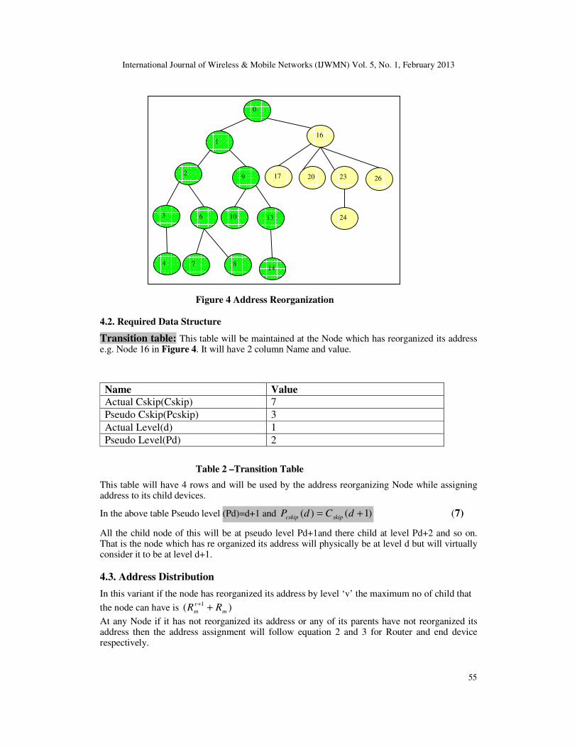
For example if node 16 goes for address reorganization as it is at level 1 its original Cskip value

is 7 but it will use its next level Cskip value i.e. level 2 which is 3, and the maximum no of child

it can have will be 2*2+2=6 and the network depth at that part will be Lm-1=3.

So after address reorganization node 16 will be able to add 4 more children. Following Figure 4

shows the structure of the network after address reorganization


55

Figure 4 Address Reorganization

4.2. Required Data Structure

Transition table: This table will be maintained at the Node which has reorganized its address e.g. Node 16 in Figure 4. It will have 2 column Name and value.

Name Value

Actual Cskip(Cskip) 7

Pseudo Cskip(Pcskip) 3

Actual Level(d) 1

Pseudo Level(Pd) 2

Table 2 –Transition Table

This table will have 4 rows and will be used by the address reorganizing Node while assigning address to its child devices.

In the above table Pseudo level (Pd)=d+1 and )1()( += dCdP skipcskip (7)

All the child node of this will be at pseudo level Pd+1and there child at level Pd+2 and so on. That is the node which has re organized its address will physically be at level d but will virtually consider it to be at level d+1.

4.3. Address Distribution

In this variant if the node has reorganized its address by level ‘v’ the maximum no of child that

the node can have is )( 1

m

v

m RR ++

At any Node if it has not reorganized its address or any of its parents have not reorganized its address then the address assignment will follow equation 2 and 3 for Router and end device respectively.

0

1 16

9 20 17 2

3 6

4 7

13 10

8 14

23 26

24


56

If the Node has reorganized its address by level ‘v’ then the address assigned to its router capable device will be as follows:

For thR routing capable child if R is <= 11

++v

mR

1)1).(( +−+=th

cskipparentRRdPAA th (8)

Else if m

v

m

v

m RRRR +<=<+++ 11 1 (9)

Then address is given by ERdPAA v

mcskipparentR th +++=+ 1)( 1

(10)

Where G= ).........( 2 v

mmm RRR ++ & for v >3

)1).(....1).(1( 112−−++++−=

+− v

m

v

mmmmm RRRRRRCE (11)

for v=1, )1).(1( 1−−+−=

+v

mmm RRRCE (12)

for v=2, )1).(1).(1( 1−−++−=

+v

mmmm RRRRCE (13)

for v=3, )1).(1).(1( 12−−+++−=

+v

mmmmm RRRRRCE (14)

These nodes will mark their relative position as 1. i.e. they are at 1 level below the node

which has reorganized its address. The child node of this node will mark its relative position as

two and so on. For example in Figure-7 Node 42 and 51 are at relative level 1, node 43, 46, 52

and 55 are at relative level two. The Cskip value for a node at relative level ‘e’ for’v’>3 is

given by

))(.......1).(1()( 2 termevuptoRRRCeR mmmmskip −++++−= (15)

for v-e=1, ).1()1( +−= mmskip RCR (16)

for v-e =2, )1).(1()1( mmmskip RRCR ++−= (17)

for v-e =3, )1).(1()1( 2

mmmmskip RRRCR +++−= (18)

Network address to the end device is given in a sequential manner and the address given to

nth end device is given by the following equation.

FnRdPAA v

mcskipParentn +++=+1).( (19)

parentofaddressisAAndRmCmn parent−≤≤1 And GRCF mm ).1( +−=

All the nodes which are descendent of first 1+v

mR child of that reorganizing node will use the

subsequent depth and Cskip values, and the node which are descendent of next Rm child will use Rskip value for address distribution. Please refer to Figure-7 for network formation. In that node 1 has reorganized its address by level 2 so the no of router capable device that can be attached to

it is 103=+ mm RR among which 8 node have Pseudo Cskip here 5=cskipP and the other 2

child Node will have Relative Cskip here the value is 933)1( =×=skipR according to

Equation 17 i.e. node & which is among 1st 8 child node will use 5=cskipP and node 42 will use

933)1( =×=skipR for address distribution.

4.4. Additional Data Structure

In this type one additional register posR will be required for storing the relative position. This

register’s value will be set only if the Rth Node is a child of the address reorganizing node and if

m

v

m

v

m RRRR +<=<++ 11

or child of a node which satisfies the above two conditions for example in Figure-7 node 42 has

posR =1 Node 43 has posR =2


57

4.5. Routing in Reorganized Network

At any Node if it has not reorganized its address then the routing will follow the normal process i.e. it will follow equation 4,5and 6. If the Node has reorganized its address then routing will be as follows:

If the destination is a descendant of the device, the device shall route the frame to the

appropriate child. If the destination is not a descendant, the device shall route the frame to its

parent. For a ZigBee router with address A at depth d, and pseudo depth Pd if the following

logical expression is true, then a destination device with address D is a descendant:

)1( −+<< dCADA skip (20)

If it is determined that the destination is a descendant of the receiving device then it is checked

if the destination is a child end device using the formula

)1.()(.1+−++>

+

mmdcskip

v

m RCGPPRAD , (21)

If it is a child end device then the address N of the next hop device is given by: N=D.

Otherwise,

If the destination address 1).( +

+<=<v

mdcskip RPPADA

then the next hop address is given by:

)()(

)1(1 dcskip

dcskip

PPPP

ADAN ×

+−++= (22)

else the next hop address is given by

)( cskip

csik

RR

ZDZN ×

−+= (23)

Where )(1 1

dcskip

v

m PPRAZ ×++=+

(23)

All the nodes which are descendent of first 1+v

mR child of that reorganizing node shall use there

pseudo depth and the node which are descendent of next Rm child shall use relative depth and relative Cskip value in place of Cskip in equation 4,5,6,7 for routing purpose, no other changes are needed .

A node will use posR register to decide if it needs to use cskipP or )(eRskip for routing. If the

posR register contains a not null value then it will use )(eRskip else it will use cskipP if it is a

descendent of address reorganized node and skipC otherwise.

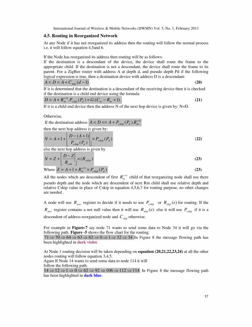
For example in Figure-7 say node 71 wants to send some data to Node 34 it will go via the following path. Figure -5 shows the flow chart for the routing.

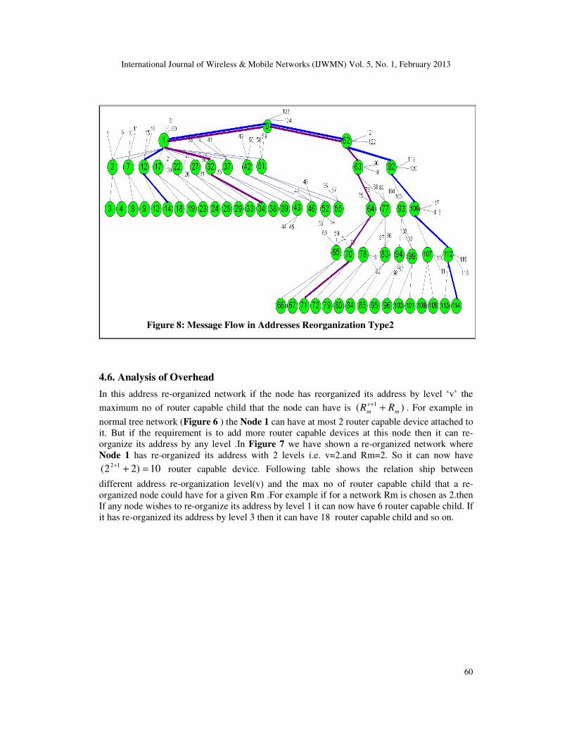
3432106263647071 ⇒⇒⇒⇒⇒⇒⇒⇒ .In Figure 8 the message flowing path has been highlighted in dark violet. At Node 1 routing decision will be taken depending on equation (20,21,22,23,24) at all the other nodes routing will follow equation 3,4,5. Again If Node 14 wants to send some data to node 114 it will follow the following path.

1141121069262011214 ⇒⇒⇒⇒⇒⇒⇒⇒ In Figure 8 the message flowing path has been highlighted in dark blue.


58

)0(skipC )1(skipC )2(skipC )3(skipC )4(skipC )5(skipC

61 29 13 5 1 0

Table 3: Cskip Value at various levels

Figure 5: Routing in address Reorganized Network


59

Figure 7: Address Distribution with Two levels Addresses Reorganization Type2

Figure 6: Address Distribution without address Reorganization


60

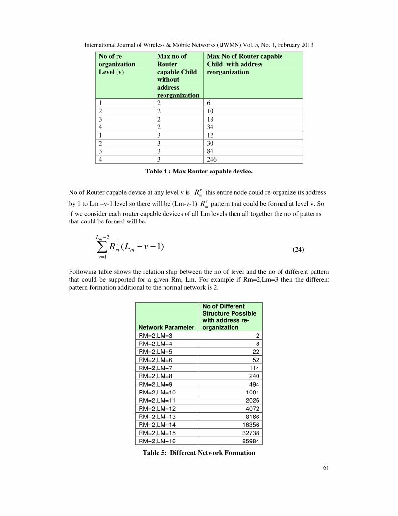
4.6. Analysis of Overhead

In this address re-organized network if the node has reorganized its address by level ‘v’ the

maximum no of router capable child that the node can have is )( 1

m

v

m RR ++

. For example in

normal tree network (Figure 6 ) the Node 1 can have at most 2 router capable device attached to

it. But if the requirement is to add more router capable devices at this node then it can re-

organize its address by any level .In Figure 7 we have shown a re-organized network where

Node 1 has re-organized its address with 2 levels i.e. v=2.and Rm=2. So it can now have

10)22( 12=+

+

router capable device. Following table shows the relation ship between

different address re-organization level(v) and the max no of router capable child that a re-

organized node could have for a given Rm .For example if for a network Rm is chosen as 2.then

If any node wishes to re-organize its address by level 1 it can now have 6 router capable child. If

it has re-organized its address by level 3 then it can have 18 router capable child and so on.

Figure 8: Message Flow in Addresses Reorganization Type2


61

No of re

organization

Level (v)

Max no of

Router

capable Child

without

address

reorganization

Max No of Router capable

Child with address

reorganization

1 2 6

2 2 10

3 2 18

4 2 34

1 3 12

2 3 30

3 3 84

4 3 246

Table 4 : Max Router capable device.

No of Router capable device at any level v is v

mR this entire node could re-organize its address

by 1 to Lm –v-1 level so there will be (Lm-v-1) v

mR pattern that could be formed at level v. So

if we consider each router capable devices of all Lm levels then all together the no of patterns

that could be formed will be.

)1(2

1

−−∑−

=

vLR m

L

v

v

m

m

(24)

Following table shows the relation ship between the no of level and the no of different pattern

that could be supported for a given Rm, Lm. For example if Rm=2,Lm=3 then the different

pattern formation additional to the normal network is 2.

Network Parameter

No of Different Structure Possible with address re-organization

RM=2,LM=3 2

RM=2,LM=4 8

RM=2,LM=5 22

RM=2,LM=6 52

RM=2,LM=7 114

RM=2,LM=8 240

RM=2,LM=9 494

RM=2,LM=10 1004

RM=2,LM=11 2026

RM=2,LM=12 4072

RM=2,LM=13 8166

RM=2,LM=14 16356

RM=2,LM=15 32738

RM=2,LM=16 85984

Table 5: Different Network Formation


62

Figure 9 : No of Different Structure Possible with address re-organization

0

10000

20000

30000

40000

50000

60000

70000

80000

90000

100000

RM

=2

,LM

=3

RM

=2

,LM

=4

RM

=2

,LM

=5

RM

=2

,LM

=6

RM

=2

,LM

=7

RM

=2

,LM

=8

RM

=2

,LM

=9

RM

=2,L

M=

10

RM

=2,L

M=

11

RM

=2,L

M=

12

RM

=2,L

M=

13

RM

=2,L

M=

14

RM

=2,L

M=

15

RM

=2,L

M=

16

No of Different StructurePossible with address re-organization

5. CONCLUSIONS

Sensornets are closely coupled to the physical world and can directly impact our Personal

Operating Space (POS). One of the major advantages of IEEE802.15.4 is that it uses free 2.4

GHz ISM band at the Physical layer. Nodes in a sensornet are low cost and the performance of

this architecture is already well-proven.

The wireless network with minimum data rate, reduced energy consumption and minimum cost

is formed by IEEE 802.15.4 standard. The distinctive characteristics of the standard makes it

more approving module for wireless sensor networks and remote monitoring applications. It

offers a minimum power, economic and a consistent protocol for wireless connectivity among

low-cost, permanent and moveable devices. These devices can figure out into a sensor network

or wireless personal area network (WPAN). After a great success in personal operating space

(POS), researchers are trying to use it in relatively broad areas such as industrial automation,

tracking and monitoring systems, public telecom services etc. This is only possible if a large

network can be formed. For this purpose it needs a suitable routing algorithm.

In this paper we have tried to mitigate the problem of symmetric structure and provided a

unique technique of address reorganization which will help the network in a variety of different

application scenarios staring from mine field to Glacier war field to building automation. The

main advantage of this algorithm is that we can form many different network with the

Lm : Max Depth

Rm: Max Router child


63

introduction of just two variable called Pseudo Cskip(Pcskip) and Pseudo Level(Pd) no other

extra overhead such as routing table will not be required.

ACKNOWLEDGEMENTS

The authors would like to thank everyone, just everyone!

REFERENCES

[1] C. E. Perkins, E. Belding-Royer, and S. R. Das, “Ad hoc On-Demand Distance Vector (AODV)

Routing”, http://www.ietf.org/rfc/rfc3561.txt, July 2003. RFC 3561.[AODV_1]

[2] C. E. Perkins and P. Bhagwat, “Highly Dynamic Destination-Sequenced Distance-Vector Routing

(DSDV) for Mobile Computers”, Proceedings of ACM SIGCOMM, 1994.[C_E_DSDV]

[3] C. E. Perkins and Elizabeth Royer, “Ad-hoc On-Demand Distance Vector Routing”, Proceedings of

the 2nd IEEE Workshop on Mobile Computing Systems and Applications, New Orleans, LA,

February 1999. [AODV_2]

[4] D. B. Johnson, D. B. Maltz, “Dynamic Source Routing in Ad-hoc Wireless Networks”, Mobile

Computing, T. Imielinski, H. Korth, Eds. Kluwer Academic Publishers, 1996, ch. 5, pp. 153-

181.[Johnson_DSR]

[5] D. Ganeshan, B. Krishnamachari, “Complex Behavior at Scale: An Experimental Study of Low-

Power Wireless Sensor Networks”, UCLA/CSD-TR 02-0013, UCLA Computer Science,

2002.[Low_Power]

[6] Debabrato Giri, Uttam Kumar Roy, “Address Borrowing In Wireless Personal Area Network”,

Proc. of IEEE International Anvanced Computing Conference, (IACC ’09, March 6-7), Patiala,

India, page no 1074-1079[ukr_borrowing]

[7] Debabrato Giri, Uttam Kumar Roy, “Single Level Address Reorganization In Wireless Personal

Area Network”, 4th International Conference on Computers & Devices for Communication

(CODEC-09), December 14-16, 2009, Calcutta University, India. [ukr_single]

[8] Ed Callaway, Paul Gorday, Lance Hester, Jose A. Gutierrez, Marco Naeve, Bob Heile and Venkat

Bahl. “Home Networking with IEEE 802.15.4: A Developing Standard for Low-Rate Wireless

Personal Area Networks”,IEEE Communications Magazine August 2002.[Low_Rate]

[9] Elizabeth Royer and C-K Toh, “A Review of Current Routing Protocols for Ad-Hoc Mobile

Wireless Networks”, IEEE Personal Communications Magazine, April 1999.[Routing_Protocols]

[10] Gang Lu, Bhaskar Krishnamachari, Cauligi S. Raghavendra, “Performance Evaluation of the IEEE

802.15.4 MAC for Low-Rate Low-Power Wireless Networks”, IEEE International Conference on

Performance, Computing, and Communications, 2004.[Performace]

[11] IEEE 802.15.11 Standard: ”Wireless Local Area Networks, 1999”. [WLAN]

[12] IEEE 802.15.1, Wireless Medium Access Control (MAC) and Physical layer (PHY) specifications

for Wireless Personal Area Networks (WPANs) [Bluetooth]

[13] IEEE 802.15.4, Wireless Medium Access Control (MAC) and Physical Layer (PHY) Specifications

for Low-Rate Wireless Personal Area Networks (WPANs) [WPAN]

[14] J. Heidemann, W. Ye and D. Estrin.”An Energy-Efficient MAC Protocol for Wireless Sensor

Networks”, Proceedings of the 21st International Conference of the IEEE Computer and

Communications Societies (INFOCOM 2002), New York, NY, June 2002.[Energy]

[15] Jianliang Zheng and Myung J. Lee. “A Comprehensive Performance Study of IEEE 802.15.4”,

http://www-ee.ccny.edu/zheng/pub, 2004. [Comprehensive]

[16] 14, C. Schurgers, S. Park and M. B. Srivastava, “Energy-Aware Wireless Microsensor Networks”,

IEEE Signal Processing Magazine, Volume: 19, Issue: 2, March 2002.[Aware]


64

[17] Shree Murthy, J. J. Garcia-Luna-Aceves, “An Efficient Routing Protocol for Wireless Networks”,

Mobile Networks and Applications, 1996.[Efficient]

[18] Uttam Kumar Roy, Debarshi Kumar Sanyal, Sudeepta Ray, "Analysis and Optimization of Routing

Protocols in IEEE802.15.4" (Asian International Mobile Computing Conference (AMOC 2006),

Jadavpur University, Kolkata, India [UKR_AMOC]

[19] ZigBee Alliance (ZigBee Document 053474r17) Draft Version 0.90: Network Specification, Jan

2008.[ZigBee]

[20] ZigBee Alliance (ZigBee Document 075307r07) Version 1.0: Telecom Applications Profile

Specification, April 2010.[ZigBee Telecom]

[21] ZigBee Alliance (ZigBee Document 053516r12) Version 1.0: ZigBee Building Automation

Application Profile, May 2011.[ZigBee Building Automation]

Authors : Debabrato Giri

Research Scholar,

Department of Information

Technology,

Jadavpur University

Authors : Uttam Kumar Roy

Currently working as an assistant professor in the Dept. of information

Technology. Jadavpur University, Kolkata, India. Has completed his Ph. D in

engineering from the same university and has nearly 10 years of teaching

experience. He is the sole author of the book entitled “Web Technologies”

published by Oxford University press in 2010. Contributed numerous research

papers to various journals.

Multilevel address reorganization type2 in wireless personal area network

Documents

Transcript of Multilevel address reorganization type2 in wireless personal area network