Multi-scale analysis of butterfly diversity in a Mediterranean mountain landscape: mapping and...

ORI GIN AL PA PER

Multi-scale analysis of butterfly diversity in aMediterranean mountain landscape: mappingand evaluation of community vulnerability

Stefano Scalercio Æ Roberto Pizzolotto ÆPietro Brandmayr

Received: 14 February 2005 / Accepted: 27 February 2006 / Published online: 3 May 2006� Springer Science+Business Media, Inc. 2006

Abstract This paper is an attempt to outline a protocol for animal diversity census and

evaluation aimed for areas in view of landscape planning of territories of hundred square

kilometres and more, that may work utilising different faunal groups and be anyway useful

at various scales. Many papers are addressed to elaborate tools for landscape planning

starting from biodiversity evaluation and butterflies are often utilised because of their

sensitivity to landscape modifications. In this work, the biodiversity evaluation has been

performed using three hierarchically linked landscape units at micro-, meso- and macro-

scale. Being species diversity values often inadequate to define the conservation interest of

a landscape portion, more importance has been given to which species compose the species

assemblages. A community vulnerability Index was coded and used for evaluating

potential consequences of human disturbance on butterfly assemblages. Forty-four year

samples were gained by visual census in the Sila Greca, Southern Italy, on an area of

approximately 520 square kilometres. During 5 years work, 2,535 specimens and 94

species were recorded, equal to 75.8% of the whole Calabrian fauna. Four vulnerability

levels have been established and used for mapping butterfly assemblage vulnerability in the

area, starting from a vegetation map. Species richness was found somewhat contradictory

at micro-scale, where the community vulnerability Index gives a sounder approach. S

diversity gives a more reliable picture of naturalness at meso-scale, a level we identified

with the ‘‘ecotope’’. At this more ‘‘geomorphic’’ scale level, biological functions reflected

by butterfly assemblages revealed to be clearly linked to seral processes. Similarity

analysis results show that the ecotope species richness, here called ‘‘eta-diversity’’, could

be an useful measure of zoological landscape (faunation) potentialities.

Keywords Butterflies Æ Diversity Æ Species assemblages Æ Vulnerability ÆLandscape scale Æ Ecotope Æ Eta-diversity Æ Landscape planning

S. Scalercio (&) Æ R. Pizzolotto Æ P. BrandmayrDepartment of Ecology, University of Calabria, Arcavacata di Rende, I-87036 Cosenza, Italye-mail: [email protected]

123

Biodivers Conserv (2007) 16:3463–3479DOI 10.1007/s10531-006-9015-z

Introduction

A large body of literature is addressed to elaborate practical tools for applying results of

biological research in conservation of natural resources and landscape planning, but in many

cases at least two problems make these tools inapplicable: (1) their relevance limited to a

single taxon and (2) the difficulty to link results to functional landscape units. Papers devoted

to conservation topics often utilise biodiversity as a tool for investigating and evaluating the

interest of an area (Magurran 1988; Gaston 1996; Conroy and Noon 1996; Myers et al. 2000)

but it is at least similarly important to take into account ecological attributes of surveyed

species assemblages (Kremen 1992). Diversity values per se, whether S or other diversity

indices, are often inadequate to define the conservation interest of a given landscape portion

(Samways 1994). Intensification of human activities, in fact, does not always lead to a

decrease in species richness (Burel et al. 1998), depending on the faunistic group surveyed

and the intensity of environmental alterations (Blair and Launer 1997). Starting from such

premises, it becomes important to evaluate which species compose species assemblages, and

the abundance they have, for carrying out correct conclusions (Kremen 1992). In this ad-

dress, the evaluation of life history traits of species could be very useful.

Several studies suggest that many faunal higher taxa may be used as surrogates and

correlates of biodiversity (Noss 1990; Duelli and Obrist 1998; Blair 1999), but each

taxonomic group has its own ecological features representing just a small functional

portion of an ecosystem. Indeed many papers involving more than one taxon are available

(e.g. Blair 1999; Soderstrom et al. 2001; Kruess and Tscharntke 2002; Jeanneret et al.

2003). Instead of a multi-taxa approach, a mono-taxon approach could be utilised in areas

monitoring and conservation studies when correctly chosen and utilised (Kremen 1992).

Butterflies were often used as bioindicators because they play important ecological roles as

herbivores, pollinators and prey, and are known to be strictly correlated to habitat diversity

(e.g. New 1991; Pollard and Yates 1993; Molina and Palma 1996; Blair and Launer 1997).

In order to avoid mistakes in ranking priority areas for conservation, it is necessary to

link the results to a functional landscape unit. Lapin and Barnes (1995) suggest a landscape

ecosystem approach to assess and map plant and ecosystem diversity. This approach,

partially followed here, is an attempt towards the individuation of nonarbitrary and

functional units in landscape ecology studies and diversity mapping, but the ecosystem

concept is unlinked to spatial scales.

In this paper, we used a hierarchically nested approach in evaluation the diversity and the

vulnerability of butterfly communities. Data registered at micro-scale, i.e. within surveyed

sites, were used to obtain data at meso-scale and macro-scale following a bottom-up

strategy. In this way, we hoped (1) to evaluate the consequences of human activities on

butterfly assemblages at various scales, and (2) to build a cartographic model of diversity. A

multi-scale approach in diversity studies is very important because diversity patterns depend

on different factors at various scales. In short, the purpose of this paper is to produce a useful

framework for landscape managing and territorial planning whatever the surface of given

territory and that works involving indifferently many faunal groups or ‘‘guilds’’.

Methods

Study area

Surveys were carried out in the Sila Greca Massif (Fig. 1), Calabria, Southern Italy. The

study area reaches a maximum height of 1,635 m a.s.l. on a surface of about 520 km2 and

3464 Biodivers Conserv (2007) 16:3463–3479

123

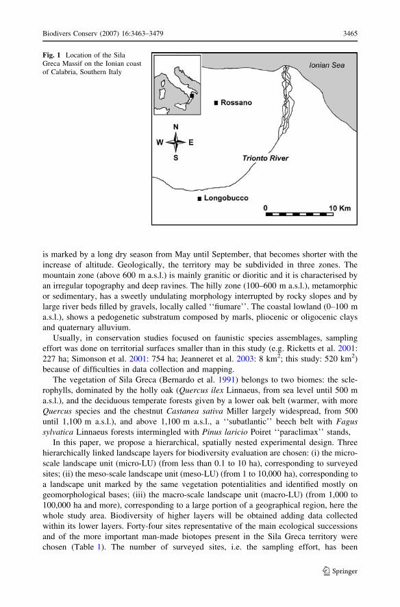
is marked by a long dry season from May until September, that becomes shorter with the

increase of altitude. Geologically, the territory may be subdivided in three zones. The

mountain zone (above 600 m a.s.l.) is mainly granitic or dioritic and it is characterised by

an irregular topography and deep ravines. The hilly zone (100–600 m a.s.l.), metamorphic

or sedimentary, has a sweetly undulating morphology interrupted by rocky slopes and by

large river beds filled by gravels, locally called ‘‘fiumare’’. The coastal lowland (0–100 m

a.s.l.), shows a pedogenetic substratum composed by marls, pliocenic or oligocenic clays

and quaternary alluvium.

Usually, in conservation studies focused on faunistic species assemblages, sampling

effort was done on territorial surfaces smaller than in this study (e.g. Ricketts et al. 2001:

227 ha; Simonson et al. 2001: 754 ha; Jeanneret et al. 2003: 8 km2; this study: 520 km2)

because of difficulties in data collection and mapping.

The vegetation of Sila Greca (Bernardo et al. 1991) belongs to two biomes: the scle-

rophylls, dominated by the holly oak (Quercus ilex Linnaeus, from sea level until 500 m

a.s.l.), and the deciduous temperate forests given by a lower oak belt (warmer, with more

Quercus species and the chestnut Castanea sativa Miller largely widespread, from 500

until 1,100 m a.s.l.), and above 1,100 m a.s.l., a ‘‘subatlantic’’ beech belt with Fagus

sylvatica Linnaeus forests intermingled with Pinus laricio Poiret ‘‘paraclimax’’ stands,

In this paper, we propose a hierarchical, spatially nested experimental design. Three

hierarchically linked landscape layers for biodiversity evaluation are chosen: (i) the micro-

scale landscape unit (micro-LU) (from less than 0.1 to 10 ha), corresponding to surveyed

sites; (ii) the meso-scale landscape unit (meso-LU) (from 1 to 10,000 ha), corresponding to

a landscape unit marked by the same vegetation potentialities and identified mostly on

geomorphological bases; (iii) the macro-scale landscape unit (macro-LU) (from 1,000 to

100,000 ha and more), corresponding to a large portion of a geographical region, here the

whole study area. Biodiversity of higher layers will be obtained adding data collected

within its lower layers. Forty-four sites representative of the main ecological successions

and of the more important man-made biotopes present in the Sila Greca territory were

chosen (Table 1). The number of surveyed sites, i.e. the sampling effort, has been

Fig. 1 Location of the SilaGreca Massif on the Ionian coastof Calabria, Southern Italy

Biodivers Conserv (2007) 16:3463–3479 3465

123

proportionally subdivided among meso-LUs looking at their surface in the study area

(Table 2). Sample sites were not randomly chosen, because both random sampling design

and stratified random sampling design were inapplicable. The dense landscape fragmen-

tation of the Sila Greca Massif could have lead to the censual exclusion of some particular

habitat from surveyed sites, and the very hard topography of the Massif made the access at

random places very difficult and time consuming. Main meso-LUs were identified by

taking into account (a) geological substrata, (b) geomorphic features, and (c) climate

conditioned vegetation (see Table 2). Meso-LUs may be ‘‘zonal’’ or ‘‘azonal’’: in zonal

meso-LU seres run up to the final stage of the ecosystem determined by climate (the

climax, in Europe mostly a forest), in azonal ones the bedrock and other physical condi-

tions as subsoil water or erosion, restrain the development of ecosystem/vegetation to early

succession stages (sand dunes, river beds, rock cliffs, etc.).

Sampling

Field work was carried out from 1993 to 1998 by investigating new sample sites each year.

Sample sites were each third week monitored from March until November, in sunny days

and between 9:30 a.m. and 3:00 p.m., inverting daily sequence of visits. If the first sam-

pling sequence of sample sites was ABC, the second was CBA, the third ABC and so on,

reducing on this way the sampling hour effects on collected data. A zigzag line was

followed during systematic walking surveys, 10 min long to limit the ingress of individuals

into the sample site. No one point of sample sites was covered more than once. A time

constrained sample has been chosen instead a surface constrained sample because of

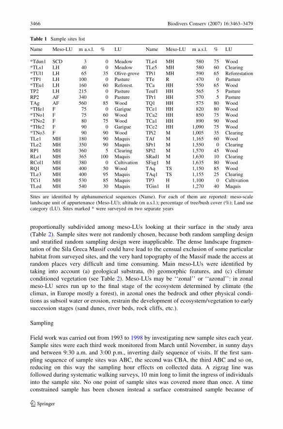
Table 1 Sample sites list

Name Meso-LU m a.s.l. % LU Name Meso-LU m a.s.l. % LU

*Tdun1 SCD 3 0 Meadow TLe4 MH 580 75 Wood*TLs1 LH 40 0 Meadow TLe5 MH 580 60 Clearing*TUl1 LH 65 35 Olive-grove TPi1 MH 590 65 Reforestation*TP1 LH 100 0 Pasture TTe R 470 0 Pasture*TEu1 LH 160 60 Reforest. TCa HH 550 65 WoodTP2 LH 215 0 Pasture Teuf1 HH 565 5 PastureRP2 AF 340 0 Pasture TPr1 HH 570 5 PastureTAg AF 560 85 Wood TQ1 HH 575 80 Wood*THe1 F 75 0 Garigue TCe1 HH 820 80 Wood*TNo1 F 75 60 Wood TCa2 HH 850 75 Wood*TNo2 F 80 75 Wood TCa1 HH 890 90 Wood*THe2 F 90 0 Garigue TCe2 HH 1,090 75 Wood*TNo3 F 90 90 Wood TPi2 M 1,005 35 ClearingTLe1 MH 180 90 Maquis TAf M 1,165 60 WoodTLe2 MH 350 90 Maquis SPr1 M 1,550 0 ClearingRP1 MH 360 5 Clearing SPi2 M 1,570 45 WoodRLe1 MH 365 100 Maquis SRad1 M 1,630 10 ClearingRCol1 MH 380 0 Cultivation SFag1 M 1,635 80 WoodRQ1 MH 400 50 Wood TAq TS 1,150 85 WoodTLe3 MH 400 95 Maquis TAq1 TS 1,155 25 ClearingTCi1 MH 530 85 Maquis TP3 H 1,100 0 CultivationTLed MH 540 30 Maquis TGin1 H 1,270 40 Maquis

Sites are identified by alphanumerical sequences (Name). For each of them are reported: meso-scalelandscape unit of appurtenance (Meso-LU); altitude (m a.s.l.); percentage of tree/bush cover (%); Land usecategory (LU). Sites marked * were surveyed on two separate years


123

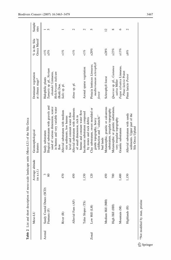
Tab

le2

Lis

tan

dsh

ort

des

crip

tio

no

fm

eso

-sca

lela

ndsc

ape

un

its

(Mes

o-L

U)

of

the

Sil

aG

reca

Mes

o-L

UA

ver

age

alti

tud

e(m

a.s.

l.)

Geo

mo

rph

olo

gic

alfe

atu

res

Do

min

ant

veg

etat

ion

atcl

imax

stag

e*%

inth

eS

ila

Gre

caM

assi

fS

amp

lesi

tes

Azo

nal

San

dy

Coas

tal

Du

nes

(SC

D)

3S

andy

sub

stra

tum

Hal

op

hil

icp

lants

<1

%1

Fiu

mar

a(F

)8

0Il

log

ical

sub

stra

tum

wit

hg

rav

els

and

san

do

fv

ario

us

dim

ensi

on

,sc

arce

inh

um

us

and

ver

yv

aria

ble

wat

erfl

ow

Ta

mari

xsp

.p

l.,

Ner

ium

ole

an

der

Lin

nae

us,

Hel

ich

rysu

mit

ali

cum

(Ro

th)

Do

n.

@5%

5

Riv

er(R

)4

70

All

uv

ial

sub

stra

tum

wit

hm

ediu

msi

zese

dim

ents

,lo

wh

um

us

lev

elan

dco

nst

ant

wat

erfl

ow

Sa

lix

sp.

pl.

<1

%1

All

uvia

lF

ans

(AF

)450

All

uvia

lsu

bst

ratu

mw

ith

sedim

ents

of

smal

ld

imen

sio

n,

rich

inh

um

us

and

con

stan

tw

ater

flo

w

Aln

us

sp.

pl.

<1

%2

Tal

us

Slo

pes

(TS

)1

,15

0In

coh

eren

tsu

bst

ratu

mco

mp

ose

db

yst

on

esan

dro

ckd

ebri

sA

zon

alsp

arse

veg

etat

ion

<1

%2

Zo

nal

Lo

wH

ill

(LH

)1

20

Cla

ysu

bst

ratu

m,

swee

tm

ou

lded

or

gen

tle

top

og

rap

hy

,h

eav

yso

lifl

uct

ion

and

‘‘ca

lan

chi’

’b

adla

nds

Pis

taci

ale

nti

scu

sL

inn

aeu

s,m

edit

erra

nea

nsc

lero

ph

yll

fore

st

@20

%5

Med

ium

Hil

l(M

H)

45

0M

etam

orp

hic

,g

ran

itic

or

calc

areo

us

sub

stra

tum

,ir

reg

ula

rto

po

gra

phy

Scl

ero

ph

yll

fore

st@2

8%

12

Hig

hH

ill

(HH

)7

00

Met

amo

rphic

or

gra

nit

icsu

bst

ratu

m,

ver

yir

reg

ula

rto

po

gra

ph

yQ

uer

cus

sp.

pl.

,C

ast

an

easa

tiva

Mil

ler

@23

%8

Mo

un

tain

(M)

1,4

00

Gra

nit

icsu

bst

ratu

mF

agus

sylv

ati

caL

inn

aeu

s,P

inu

sla

rici

oP

oir

et@1

3%

6

Hig

hla

nds

(H)

1,1

50

All

uv

ial

sub

stra

tum

wit

hsa

nd

yse

dim

ents

.U

pp

erp

art

of

the

Sil

aG

reca

Up

land

Pin

us

lari

cio

Po

iret

@8%

2

*N

ot

mo

difi

edb

ym

an,

pri

stin

e


123

difficulties to find biotopes sufficiently large and homogeneous for diluting discontinuity in

the distribution of populations.

In order to estimate population changes and influence of chance on results ten sites (see

Table 1) were surveyed on two separate years, while, in order to know community

modifications during the day, a pasture (TP1) was surveyed at 9:00/10:00 a.m., 12:00/1:00

p.m., 2:00/3:00 p.m.

Individuals found at boundary of stands are not registered. Specimens were identified in

the field and immediately released. The species were named according to Balletto and

Cassulo (1995).

Data analysis

A species/sample sites matrix (MS/S) constructed by using the registered individual

number (N), was the data source for any further analysis. Qualitative (QS) and quantitative

percentage (PS) similarity indices were used to compare species assemblages (see Hanski

and Koskela 1977). The qualitative similarity index is a binary measure based on presence/

absence data, QS=2c/(a+b), in which c equals the number of species present in both

samples, a equals the number of species present in sample 1, b equals the number of

species present in sample 2 (Sørensen 1948). The percentage similarity index is based on

the coverage of a species in a sample, PS=S minimum (pi1, pi2), in which pi1 equals the

proportion of species i in sample 1, and pi2 equals the proportion of species i in sample 2

(Renkonen 1938). Both index values were expressed in percentages.

The Canonical Correspondence Analysis (CCA) was carried out by using STATISTICA

5.5 (StatSoft Italia 1999). This constrained ordination technique permits to individuate ‘‘a

posteriori’’ which environmental parameters drive species distributions. Environmental

variables are theoretically identified with the extracted dimensions (D) (or axis) by using

species ecology and variables of surveyed sites. An inertia value, associated to each

dimension, explains the percentage of the total variance in species distribution attributable

to each dimension.

Spearman rank correlation (rs) and Pearson correlation (rp) was computed by Systat

version 9.0 (SPSS 1998).

Main life history traits of species were taken into account. In particular, mobility ranges

and fundamental ecological categories proposed by Balletto and Kudrna (1985), partly

modified because of the different habitat affinity shown by some species in Calabria, were

considered the most important life history traits from a conservation viewpoint (Scalercio

2002). Mobility range (MR) vary from 1 for sedentary species to 5 for migrant species.

Species have been assigned to the following fundamental ecological categories: mesoph-

ilous (M), thermophilous (T), eurytopic (E), sciophilous (S), xerophilous (X).

Diversity analysis were performed by using ESTIMATES5 (Colwell 1997). Species

richness (S), Shannon’s index (H¢) and Simpson’s index (k) were chosen as diversity

measures. We selected Shannon’s and Simpson’s indices because relatively easy to

interpret ecologically, widely used and less sensitive to rare species and sample sizes

(Magurran 1988). The same program estimated total species richness of study area (for

complete list and explanation of estimate indices see Colwell (1997)) and constructed

rarefaction curves (species/sample sites and species/individuals) after 50 sample ran-

domisations.

In order to evaluate landscape naturalness, we computed a community vulnerability

Index (Iv) integrating information from Shannon’s index (H¢) with some autoecological

parameters, linking descriptive to functional data. First, it is important to valuate responses


123

of species to human activities. Indeed, communities may be composed mainly by highly

mobile species (capable to escape consequences of environment alterations), or by eury-

topic species (capable to adapt to live in contiguous biotopes). Species mobility is an

important measure of species vulnerability as underlined in Pollard and Yates (1993).

Mobility (M) and eurytopy (E) of comunities were computed on the basis of species

contributes as follows:

M ¼ RðpiMRiÞ

where:

pi is proportion of individuals of the species i in the assemblage;

MRi is mobility range of species i

E ¼ RPe

where Pe is proportion of individuals of eurytopic species in the assemblage.

In conclusion, we propose the following equation:

Iv ¼ ðH 0=MÞ � 2E

where:

Iv is community vulnerability Index

H¢ is Shannon’s index value of species assemblage

M is mobility of species assemblage

E is eurytopy of species assemblage

In this equation the importance of eurytopic species was emphasized, because they may

take greater benefits from human activities than species having high mobility.

Results

Reliability of collected data

Different year samples of the same stand show similarity patterns variable from 14.3% to

76.5%. Both similarity indices are positively correlated with numbers of individuals col-

lected in each sample site (QS: rs = 0.66, n = 10, p = 0.019; PS: rs = 0.74, n=10, p=0.07).

In ‘‘pseudo-communities’’ composed by few specimens, collected data are strongly

influenced by chance, while assemblages marked by high abundance values show more

durable and characteristic species structures. As a consequence, species assemblages

composed by few individuals have a low reliability and all conclusions about them have no

real statistical significance.

TP1 species assemblages monitored at various times of the day, show well-defined

patterns. Morning samples are the most abundant and rich (S = 8, H¢ = 2.79); just one

species, Polyommatus icarus, was found three times; the 50% of species (Stot=12) were

found at least twice. Taxa found only once attain low abundance values (no more than

three individuals) belonging to the species assemblage tail.

Rarefaction curves of sample sites and individuals have shown that one half of the

sample sites was sufficient to collect 87.6–3.8% of species, while sampling half of the


123

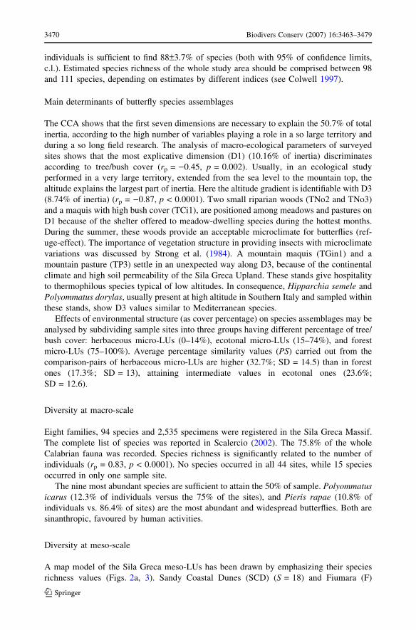
individuals is sufficient to find 88–3.7% of species (both with 95% of confidence limits,

c.l.). Estimated species richness of the whole study area should be comprised between 98

and 111 species, depending on estimates by different indices (see Colwell 1997).

Main determinants of butterfly species assemblages

The CCA shows that the first seven dimensions are necessary to explain the 50.7% of total

inertia, according to the high number of variables playing a role in a so large territory and

during a so long field research. The analysis of macro-ecological parameters of surveyed

sites shows that the most explicative dimension (D1) (10.16% of inertia) discriminates

according to tree/bush cover (rp = )0.45, p = 0.002). Usually, in an ecological study

performed in a very large territory, extended from the sea level to the mountain top, the

altitude explains the largest part of inertia. Here the altitude gradient is identifiable with D3

(8.74% of inertia) (rp = )0.87, p < 0.0001). Two small riparian woods (TNo2 and TNo3)

and a maquis with high bush cover (TCi1), are positioned among meadows and pastures on

D1 because of the shelter offered to meadow-dwelling species during the hottest months.

During the summer, these woods provide an acceptable microclimate for butterflies (ref-

uge-effect). The importance of vegetation structure in providing insects with microclimate

variations was discussed by Strong et al. (1984). A mountain maquis (TGin1) and a

mountain pasture (TP3) settle in an unexpected way along D3, because of the continental

climate and high soil permeability of the Sila Greca Upland. These stands give hospitality

to thermophilous species typical of low altitudes. In consequence, Hipparchia semele and

Polyommatus dorylas, usually present at high altitude in Southern Italy and sampled within

these stands, show D3 values similar to Mediterranean species.

Effects of environmental structure (as cover percentage) on species assemblages may be

analysed by subdividing sample sites into three groups having different percentage of tree/

bush cover: herbaceous micro-LUs (0–14%), ecotonal micro-LUs (15–74%), and forest

micro-LUs (75–100%). Average percentage similarity values (PS) carried out from the

comparison-pairs of herbaceous micro-LUs are higher (32.7%; SD = 14.5) than in forest

ones (17.3%; SD = 13), attaining intermediate values in ecotonal ones (23.6%;

SD = 12.6).

Diversity at macro-scale

Eight families, 94 species and 2,535 specimens were registered in the Sila Greca Massif.

The complete list of species was reported in Scalercio (2002). The 75.8% of the whole

Calabrian fauna was recorded. Species richness is significantly related to the number of

individuals (rp = 0.83, p < 0.0001). No species occurred in all 44 sites, while 15 species

occurred in only one sample site.

The nine most abundant species are sufficient to attain the 50% of sample. Polyommatus

icarus (12.3% of individuals versus the 75% of the sites), and Pieris rapae (10.8% of

individuals vs. 86.4% of sites) are the most abundant and widespread butterflies. Both are

sinanthropic, favoured by human activities.

Diversity at meso-scale

A map model of the Sila Greca meso-LUs has been drawn by emphasizing their species

richness values (Figs. 2a, 3). Sandy Coastal Dunes (SCD) (S = 18) and Fiumara (F)


123

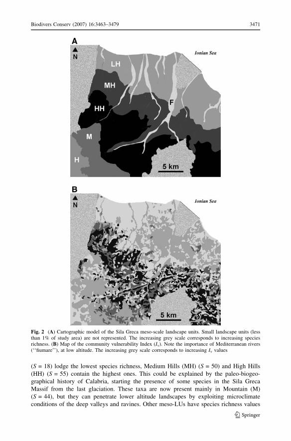
(S = 18) lodge the lowest species richness, Medium Hills (MH) (S = 50) and High Hills

(HH) (S = 55) contain the highest ones. This could be explained by the paleo-biogeo-

graphical history of Calabria, starting the presence of some species in the Sila Greca

Massif from the last glaciation. These taxa are now present mainly in Mountain (M)

(S = 44), but they can penetrate lower altitude landscapes by exploiting microclimate

conditions of the deep valleys and ravines. Other meso-LUs have species richness values

Fig. 2 (A) Cartographic model of the Sila Greca meso-scale landscape units. Small landscape units (lessthan 1% of study area) are not represented. The increasing grey scale corresponds to increasing speciesrichness. (B) Map of the community vulnerability Index (Iv). Note the importance of Mediterranean rivers(‘‘fiumare’’), at low altitude. The increasing grey scale corresponds to increasing Iv values


123

comprised between 32 and 44. The comparison of hills shows the Lower Hill (LH)

(S = 35) poorer in species than other hill meso-LUs. All the ten recognised meso-LUs bear

at least one unique species (Su), but in many cases because of stochastic reasons. Just

within High Hill (Su=3), the least man modified, and within Mountain (Su=6), because of

its above remembered paleo-biogeographical history, the unique species are significantly

more numerous.

Medium Hill and High Hill share the most species (Table 3). A number of mesophilous

elements are shared by these meso-LUs because their climax ecosystem stages are both

deciduous forest, which create similar abiotic conditions. The least similar meso-LUs are

the azonal ones, as response to their peculiar environmental conditions. Medium Hill

shares the most species with other meso-LUs having in average QS=58.3% (SD = 11.6). In

fact, Medium Hill (MH) is rich in open, more or less scattered herbaceous habitats,

inhabited by unspecialised assemblages of mobile species. In addition, MH borders on the

most meso-LUs (eight), so that individuals migrate easily from one to the neighbouring

Fig. 3 Model of the Sila Greca territory reporting meso-LUs, their schematic vegetal cover and their maindata. Double-arrows: percentage similarity (PS) between contiguous meso-LUs; black numbers: speciesrichness and (unique species). The increasing grey scale corresponds to increasing species richness

Table 3 Similarity (%) by qualitative (QS) (above the diagonal) and quantitative (PS) (below the diagonal)similarity indices for all combination-pairs of all meso-LUs

Meso-LU SCD F R AF TS LH MH HH M H

SCD – 50 48.1 38.5 32 60.4 38.2 38.4 35.5 38.6F 44 – 48.1 34.6 28 60.4 47.1 35.6 25.8 35.1R 40 47.1 – 60 44.1 64.8 65.1 61.5 47.5 53.3AF 14.7 20.5 24.5 – 51.5 49.3 66.7 62.9 51.3 57.5TS 16.4 15.9 24.6 37.9 – 41.8 53.7 52.9 50 56.3LH 48 60.8 55 23.7 18.3 – 63.5 57.8 40.5 59.5MH 43.6 47.7 43.9 44.7 28.9 57.5 – 76.2 51.1 60.7HH 32.4 40.1 42.2 35.5 31 48 53.8 – 54.5 66M 24.1 16.5 26.6 26.1 35.1 22.6 24.3 29.1 – 55.4H 19.3 27.4 32.1 34.6 28.8 36 35.8 54.7 30.9 –

Highest similarity values recorded for each meso-LU are in bold


123

unit. Very interestingly Highlands show higher QS values when compared with hilly meso-

LUs than with the contiguous Mountain (Table 3). In this case, the higher presence of

human-modified landscapes and the moderately continental climate with dryer and hotter

summer within Highlands can explain this similarity pattern.

Looking at percentage similarity, Lower Hill and Fiumara show the most similar species

assemblage (Table 3). During the summer some grassland species penetrate into Fiumara

searching for refuges from the sun into small riparian oleander woods on the ‘fiumara’ bed.

Moreover, Lower Hill and Fiumara are homogenised by summer aridity, both loosing any

alimentary sources for adults. The least similar species assemblages inhabit Sandy Coastal

Dunes (dry, soil nutrient poor, open formations) and Alluvial Fans (moist, soil nutrient

rich, forest formations), because of their extremely different environmental conditions.

Other considerations about PS affinities are the same made about QS. QS and PS show only

one important difference. Higher similarity values are always attained by QS, demon-

strating PS helpful in searching differences among species assemblages. In definitive, using

PS it is possible to discriminate assemblages taking into account the functional role as-

sumed by each species.

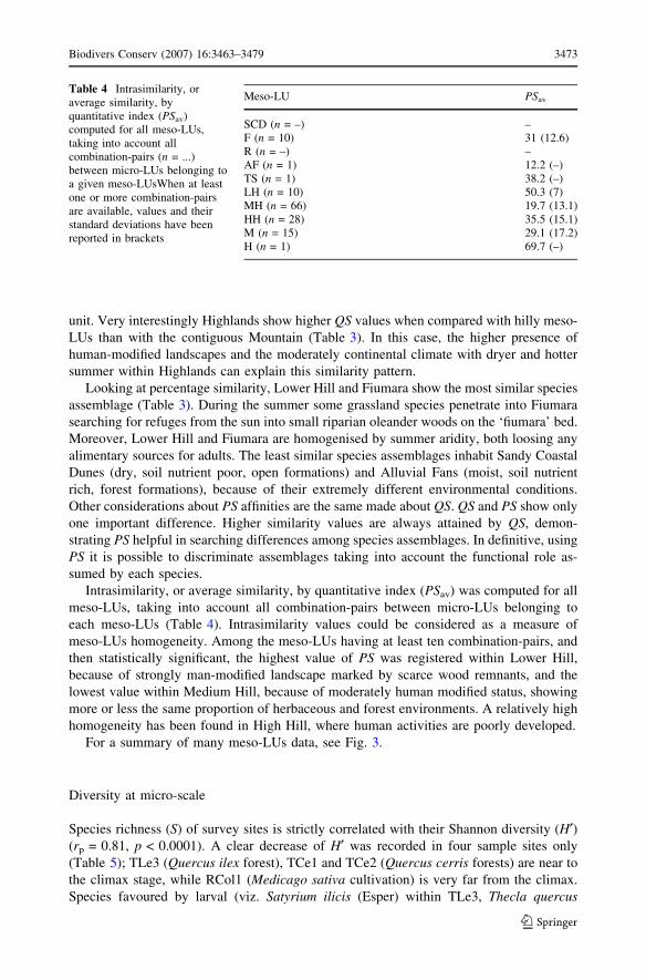
Intrasimilarity, or average similarity, by quantitative index (PSav) was computed for all

meso-LUs, taking into account all combination-pairs between micro-LUs belonging to

each meso-LUs (Table 4). Intrasimilarity values could be considered as a measure of

meso-LUs homogeneity. Among the meso-LUs having at least ten combination-pairs, and

then statistically significant, the highest value of PS was registered within Lower Hill,

because of strongly man-modified landscape marked by scarce wood remnants, and the

lowest value within Medium Hill, because of moderately human modified status, showing

more or less the same proportion of herbaceous and forest environments. A relatively high

homogeneity has been found in High Hill, where human activities are poorly developed.

For a summary of many meso-LUs data, see Fig. 3.

Diversity at micro-scale

Species richness (S) of survey sites is strictly correlated with their Shannon diversity (H¢)(rp = 0.81, p < 0.0001). A clear decrease of H¢ was recorded in four sample sites only

(Table 5); TLe3 (Quercus ilex forest), TCe1 and TCe2 (Quercus cerris forests) are near to

the climax stage, while RCol1 (Medicago sativa cultivation) is very far from the climax.

Species favoured by larval (viz. Satyrium ilicis (Esper) within TLe3, Thecla quercus

Table 4 Intrasimilarity, oraverage similarity, byquantitative index (PSav)computed for all meso-LUs,taking into account allcombination-pairs (n = ...)between micro-LUs belonging toa given meso-LUsWhen at leastone or more combination-pairsare available, values and theirstandard deviations have beenreported in brackets

Meso-LU PSav

SCD (n = –) –F (n = 10) 31 (12.6)R (n = –) –AF (n = 1) 12.2 (–)TS (n = 1) 38.2 (–)LH (n = 10) 50.3 (7)MH (n = 66) 19.7 (13.1)HH (n = 28) 35.5 (15.1)M (n = 15) 29.1 (17.2)H (n = 1) 69.7 (–)


123

(Linnaeus) within TCe1 and TCe2) or adult feeding behaviour (Polyommatus icarus and

Colias crocea (Geoffroy) within RCol1) dominate these species assemblages. Forests,

whatever their origin, almost never show species richness values higher than meadows,

pastures, or clearings (Table 5).

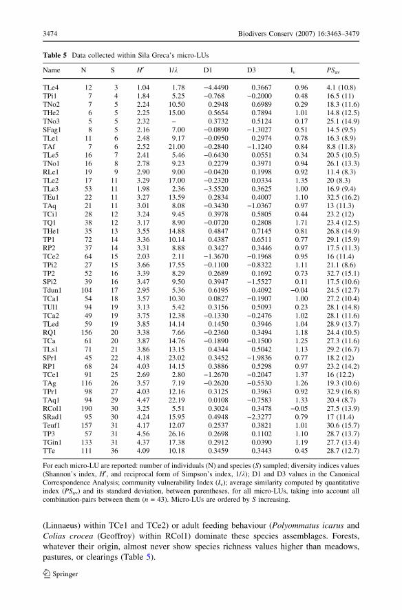
Table 5 Data collected within Sila Greca’s micro-LUs

Name N S H¢ 1/k D1 D3 Iv PSav

TLe4 12 3 1.04 1.78 )4.4490 0.3667 0.96 4.1 (10.8)TPi1 7 4 1.84 5.25 )0.768 )0.2000 0.48 16.5 (11)TNo2 7 5 2.24 10.50 0.2948 0.6989 0.29 18.3 (11.6)THe2 6 5 2.25 15.00 0.5654 0.7894 1.01 14.8 (12.5)TNo3 5 5 2.32 – 0.3732 0.5124 0.17 25.1 (14.9)SFag1 8 5 2.16 7.00 )0.0890 )1.3027 0.51 14.5 (9.5)TLe1 11 6 2.48 9.17 )0.0950 0.2974 0.78 16.3 (8.9)TAf 7 6 2.52 21.00 )0.2840 )1.1240 0.84 8.8 (11.8)TLe5 16 7 2.41 5.46 )0.6430 0.0551 0.34 20.5 (10.5)TNo1 16 8 2.78 9.23 0.2279 0.3971 0.94 26.1 (13.3)RLe1 19 9 2.90 9.00 )0.0420 0.1998 0.92 11.4 (8.3)TLe2 17 11 3.29 17.00 )0.2320 0.0334 1.35 20 (8.3)TLe3 53 11 1.98 2.36 )3.5520 0.3625 1.00 16.9 (9.4)TEu1 22 11 3.27 13.59 0.2834 0.4007 1.10 32.5 (16.2)TAq 21 11 3.01 8.08 )0.3430 )1.0367 0.97 13 (11.3)TCi1 28 12 3.24 9.45 0.3978 0.5805 0.44 23.2 (12)TQ1 38 12 3.17 8.90 )0.0720 0.2808 1.71 23.4 (12.5)THe1 35 13 3.55 14.88 0.4847 0.7145 0.81 26.8 (14.9)TP1 72 14 3.36 10.14 0.4387 0.6511 0.77 29.1 (15.9)RP2 37 14 3.31 8.88 0.3427 0.3446 0.97 17.5 (11.3)TCe2 64 15 2.03 2.11 )1.3670 )0.1968 0.95 16 (11.4)TPi2 27 15 3.66 17.55 )0.1100 )0.8322 1.11 21.1 (8.6)TP2 52 16 3.39 8.29 0.2689 0.1692 0.73 32.7 (15.1)SPi2 39 16 3.47 9.50 0.3947 )1.5527 0.11 17.5 (10.6)Tdun1 104 17 2.95 5.36 0.6195 0.4092 )0.04 24.5 (12.7)TCa1 54 18 3.57 10.30 0.0827 )0.1907 1.00 27.2 (10.4)TUl1 94 19 3.13 5.42 0.3156 0.5093 0.23 28.1 (14.8)TCa2 49 19 3.75 12.38 )0.1330 )0.2476 1.02 28.1 (11.6)TLed 59 19 3.85 14.14 0.1450 0.3946 1.04 28.9 (13.7)RQ1 156 20 3.38 7.66 )0.2360 0.3494 1.18 24.4 (10.5)TCa 61 20 3.87 14.76 )0.1890 )0.1500 1.25 27.3 (11.6)TLs1 71 21 3.86 13.15 0.4344 0.5042 1.13 29.2 (16.7)SPr1 45 22 4.18 23.02 0.3452 )1.9836 0.77 18.2 (12)RP1 68 24 4.03 14.15 0.3886 0.5298 0.97 23.2 (14.2)TCe1 91 25 2.69 2.80 )1.2670 )0.2047 1.37 16 (12.2)TAg 116 26 3.57 7.19 )0.2620 )0.5530 1.26 19.3 (10.6)TPr1 98 27 4.03 12.16 0.3125 0.3963 0.92 32.9 (16.8)TAq1 94 29 4.47 22.19 0.0108 )0.7583 1.33 20.4 (8.7)RCol1 190 30 3.25 5.51 0.3024 0.3478 )0.05 27.5 (13.9)SRad1 95 30 4.24 15.95 0.4948 )2.3277 0.79 17 (11.4)Teuf1 157 31 4.17 12.07 0.2537 0.3821 1.01 30.6 (15.7)TP3 57 31 4.56 26.16 0.2698 0.1102 1.10 28.7 (13.7)TGin1 133 31 4.37 17.38 0.2912 0.0390 1.19 27.7 (13.4)TTe 111 36 4.09 10.18 0.3459 0.3443 0.45 28.7 (12.7)

For each micro-LU are reported: number of individuals (N) and species (S) sampled; diversity indices values(Shannon’s index, H¢, and reciprocal form of Simpson’s index, 1/k); D1 and D3 values in the CanonicalCorrespondence Analysis; community vulnerability Index (Iv); average similarity computed by quantitativeindex (PSav) and its standard deviation, between parentheses, for all micro-LUs, taking into account allcombination-pairs between them (n = 43). Micro-LUs are ordered by S increasing.


123

Azonal stands have seven unique species. Five of these are interesting from a faunistic

viewpoint (Pyrgus carthami, Gegenes nostradamus, Lycaeides abetonica, Polyommatus

daphnis, Danaus chrysippus). In addition, four species (Pieris edusa, Anthocaris damone,

Hyponephele lupina, Pararge aegeria) achieve their maximum abundance in azonal bio-

topes, which act as dispersion centres. However, this observation should not be overem-

phasized. In fact, in summer high individual and species concentration occur along rivers

and puddles, due to abundant and protracted flowering favoured by the prolonged presence

of water. This fraction of the Sila Greca diversity is ecologically very fragile because of the

small surfaces of suitable landscape units (Table 2).

Zonal stands have many more unique species (30) than azonal ones, thank to their great

environmental heterogeneity along ecological successions, as well as to larger areas

covered. Standard characteristics of these species are medium or low dispersal ability,

habitat preferences for forest, and close feeding relations with near-to-climax vegetation

(Satyrium ilicis, Thecla quercus, etc.). However, this group of species contains only three

important species from a conservation viewpoint, i.e. Melanargia arge, included in the

Annex II of the EC 92/43/EEC Habitat (1992), Zerynthia polyxena, included in the Annex

IV of the same directive, and Melitaea aetherie, endangered at Italian national scale

(Balletto and Cassulo 1995).

Micro-LUs species assemblages are more variable than meso-LUs, PS varying from 0%,

to more than 65%. PS values equal to zero have been mostly registered for comparison-

pairs including (1) near-to-climax micro-LUs belonging to different meso-LUs, or (2) near-

to-climax and far-to-climax micro-LUs belonging to different meso-LUs, while the highest

PS values have been often registered between near-to-climax or between far-to-climax

micro-LUs belonging to the same meso-LUs. Among surveyed sites, the less similar in

average at all are the azonal, near-to-climax and mountain micro-LUs, that show the best

characterised species assemblages (Table 5).

Evaluation of community vulnerability

Results of the community vulnerability Index (Iv) have been reported in Table 5. We

subdivided stands into four vulnerability categories, according to increasing Iv values: no

vulnerable (Iv £ 0.39), low vulnerable (0.40 £ Iv £ 0.79), average vulnerable

(0.80 £ Iv £ 1.19) and high vulnerable (Iv ‡ 1.20). The No vulnerable category includes

mainly tilled lands, pastures and secondary formations, or micro-LUs having communities

composed by very few individuals. The Low vulnerable category includes reforestation

sites, meadows and pastures contiguous to near-to-climax formations, or stands embedded

into a well-preserved environmental matrix. The Average vulnerable category includes the

mature forests and clearings of various origin. The High vulnerable category includes only

the mature forests and the clearings of a natural origin, as well as the ‘‘precious’’ talus

slopes. This subdivision is probably arbitrary and results may be different for different

landscapes. Results, however, remain useful for comparative evaluations within a given

study area. A cartographic model of the distribution of community vulnerability was

obtained by transposing results on a vegetation map (Bernardo et al. 1991) and grouping

vegetation categories according to Iv values (Fig. 2b).

The greatest total vulnerability was recorded in the deciduous oak belt, where the

assemblages were composed, more than in other areas, by species closely related to forest

for food requirements and where human activities are limited by the rugged topography.

The smallest vulnerability was recorded within the sclerophyll biome, where the assem-

blages were composed mainly by highly mobile taxa most with polyphagous caterpillars


123

and eurytopic adults. In other words, these assemblages show the consequences of human

disturbance caused by increasing urbanisation and by intense ecosystem exploitation. At

low altitude Iv values of the ‘‘fiumare’’ are relatively high. Iv values of Subatlantic Fagus-

belt are low, probably because of the absence, in S. Italy, of species linked by feeding

relations to the pine and beech forests. Human exploitation of the environment becomes

the main factor influencing Iv values within hilly landscape units.

Discussion

Diversity analysis at micro-scale show that (1) few species dominate the species assem-

blage in some near-to-climax micro-LUs, and (2) human-modified micro-LUs often con-

tain higher diversity than near-to-climax ones. At the light of these data, it is clear that

diversity is inadequate to evaluate the conservation interest of a given micro-LUs, because

the high availability of food sources for adult butterflies in herbaceous landscape units, and

high mobility of meadow-living species lead to have this apparently contradictory diversity

pattern. At this scale indeed the relation ‘‘high diversity–high conservation interest’’

sounds inadequate. The community vulnerability index (Iv) takes into account main life

history traits of species (dispersal ability and niche choice) becoming very similar to a

measure of ‘‘typicalness’’, drawn from contextual evaluation of both diversity and auto-

ecological data inherent in species composing butterfly assemblages. In Samways’ opinion

(1994) ‘‘typicalness is probably more appropriate in the evaluation processes than is

richness’’. Maes and Van Dyck (2001) demonstrate that species having low dispersal

abilities decrease in agricultural landscape, Bergman et al. (2004) that ‘‘more mobile

species were significantly less demanding in regard to the amount of deciduous forest/

semi-natural grassland’’. The cartographic output obtained by the Iv mapping is in strong

agreement with the conclusions of these authors. The cartographic model of landscape

vulnerability of Sila Greca, with respect to human activities, based on Iv, is very similar to

a ‘‘naturalness’’ map, because species assemblages show low vulnerability when located in

perturbed environments. Very simple cartographic transposition and the simple conceptual

comprehension of Iv make this index a useful tool for local decision-makers as concerns

landscape planning and conservation goals.

Similarity analysis at micro- and meso-scale demonstrate the identity of meso-LUs from

a species assemblage viewpoint and the functional value of this landscape unit, mainly at

near-to-climax successional stages. Moreover, diversity values, sometimes contradictory at

micro-scale, give good insight into naturalness at meso-scale. The low species richness

values of Sandy Coastal Dunes and Fiumara meso-LUs (Fig. 3) are satisfactorily explained

by their extreme environmental conditions for butterfly assemblages (low fresh water

availability, and poor vegetal biomass), but human activities play also an important role,

mainly in the impoverishment of vegetation cover. In fact, many towns and beach resorts

are built along sandy coasts and near rivers. Moreover, water drainages are done for field

watering, diminishing water disposal for vegetation. The impact of human activities is

particularly evident in Low Hill meso-LU, being here the desertification process strongly

favoured. In fact, hilly meso-LUs show a very low resilience, because of the low annual

rain-falls and the low disposal of organic matter in the soil. Thus, man made environments,

such as extensive cereal and citrus cultivations, are decisive in justify a 30% diversity loss

within Low Hill in comparison to Medium Hill and High Hill meso LUs, where many

natural patches are present (Fig. 3). The meso-LUs allows us to carry out conclusions only

on the simple species number, because they represent functional landscape portions


123

individuated by using attributes objectively recognizable. As confirmed by similarity

analysis, meso-LUs are very similar to true functional landscape unit. Probably, this is the

nonarbitrary scale, invoked by Wiens (1989), at which biological function are clearly

linked to seral processes that begin and end ‘inside’ (Brandmayr et al. 1998). Attempts

towards the search of nonarbitrary scales in landscape studies, were previously done by

other authors (Lapin and Barnes 1995: plants) (for a review see Mackey et al. 2001), but

just little attention was devoted to dynamic trends inside the functional landscape unit, and

towards the development of an evaluation protocol simple to apply for non specialists too.

While our micro-LU is easily identifiable with the biotope and the related diversity with

the alpha-diversity (Cody 1975; Whittaker 1975), and our macro-LU is more or less

identifiable with the regional scale and the related gamma- (Cody 1975) or epsilon-

diversity (Witthaker 1977), some problems rise in the identification of our meso-LU. The

most similar landscape unit is the ecotope, defined by Forman and Godron (1986) as

‘‘the smallest possible land unit, that is still a holistic unit’’. Brandmayr et al. (1998) gave

to the ecotope the following definition: ‘‘a basic landscape unit delimited mostly by its

particular geomorphology, and guesting a certain number of more or less closely inter-

related ecosystem (vegetation, faunal community) types, that built a well defined com-

munity complex’’, emphasizing the importance of geomorphologic features and the

dynamic relations among vegetation and animal seral communities. Brandmayr et al.

(1998) proposed the eta-diversity (greek letter: g) as related biodiversity measurement. Eta-

diversity and Iv values show a concordant distribution pattern in the Sila Greca territory

(Fig. 2). Eta-diversity numbers have a very similar distribution of Iv values, we could

imagine the former the ‘before’ and the latter the ‘after’ the beginning of landscape

modifications by humans. Iv underlines the conditions in which ecotopes currently are, i.e.

very fragmented, composed mostly by herbaceous formations (pastures, clearings and

tilled-land of anthropic origin, often showing high species richness), surrounding forest

isles (most with low species richness).

Conclusions

In this paper, butterfly assemblages were the tool, not the goal, of a research addressed to

map areas vulnerable to human alterations. Usually, the faunistic component is the goal

and landscape attributes the tool of a research. In our approach, the presence of endangered

species for evaluating conservation interest of a given area is not strictly necessary. Indeed,

taking into account the vulnerability of species assemblages by using the community

vulnerability Index could be useful to prevent, or at least limit, local extinctions having

broad implications for conservation planning.

Our bottom-up approach (micro-to-macro) for linking biodiversity of different land-

scape scales seems to be useful in conservation strategies, because very simple to apply

over thousands of hectares, providing at the same time an effective framework for com-

paring and assessing the diversity of species assemblages within different landscape units.

In particular, the cartographic transposition of eta-diversity is very easy to practice and it

fits to a meso-scale landscape unit, here identified with the ecotope, that has more or less

homogeneous zoological potentialities. In other words, at this scale patterns and processes

seems to be strictly linked as proposed by Hobbs (1997), proving that this approach to

landscape ecology is useful for conservation science. Anyway, studies on further animal

groups are needed to give more support to the model of alpha-, eta- and gamma-diversity

proposed here.


123

Acknowledgements We thank two anonymous advisors for their constructive comments and MatthewSimonds for the English revision of the manuscript.

References

Balletto E, Cassulo LA (1995) Lepidoptera Hesperioidea, Papilionoidea. In: Minelli A, Ruffo S, La Posta S(eds) Checklist delle specie della fauna italiana, 89. Calderini, Bologna

Balletto E, Kudrna O (1985) Some aspects of the conservation of butterflies in Italy, with recommendationsfor a future strategy. Bollettino della Societa entomologica Italiana 117:39–59

Bergman K-O, Askling J, Ekberg O, Ignell H, Wahlman H and Milberg P (2004) Landscape effects onbutterfly assemblages in an agricultural region. Ecography 27:619–628

Bernardo L, Cesca G, Codogno M, Fascetti S, Puntillo D (1991) Studio fitosociologico e cartografia dellavegetazione della Sila Greca (Calabria). Studia Geobotanica 11:77–102

Blair RB (1999) Birds and butterflies along an urban gradient: surrogate taxa for assessing biodiversity?Ecol Appl 9:164–170

Blair RB, Launer AE (1997) Butterfly diversity and human land use: species assemblages along an urbangradient. Biol Conserv 80:113–125

Brandmayr P, Scalercio S, Zetto T and Pizzolotto R (1998) Carabid population and community features asan ‘adaptation’ to the landscape system: Importance of the ecotope as a landscape unit. In: BaumgartnerJ, Brandmayr P and Manly BFJ (eds) Population and community ecology for insect management andconservation. Balkema, Rotterdam, pp 227–242

Burel F, Baudry J, Butet A, Clergeau P, Delettre Y, Le Couer D, Dubs F, Morvan N, Paillat G, Petit S,Thenail C, Brunel E and Lefeuvre JC (1998) Comparative biodiversity along a gradient of agriculturallandscapes. Acta Oecol 19:47–60

Cody ML (1975) Towards a theory of continental species diversities: bird distributions over Mediterraneanhabitat gradients. In: Cody ML and Diamond JM (eds) Ecology and evolution of communities. HarwardUniversity Press, Cambridge, MA, pp 214–257

Colwell RK (1997) Estimates: Statistical estimation of species richness and shared species from samples.Version 5. User’s Guide and application published at: http://viceroy.eeb.uconn.edu/estimates

Conroy MJ, Noon BR (1996) Mapping of species richness for conservation of biological diversity: con-ceptual and methodological issues. Ecol Appl 6:763–773

Council Directive 92/43/EEC Habitat (1992) Official Journal of the European Communities, 22th July 1992Duelli P, Obrist MK (1998) In search of the best correlates for local organismal biodiversity in cultivated

areas. Biodiv Conserv 7:297–309Forman RTT and Godron M (1986) Landscape ecology. John Wiley and Sons, New YorkGaston KJ (1996) Species richness: measure and measurement. In: Gaston KJ (eds) Biodiversity: a biology

of numbers and difference. Blackwell Science, Oxford, pp 77–113Hanski I and Koskela H (1977) A re-examination of a debate on methods of ecological classification in

Finland in the 1940s. Ann Entomol Fennicae 43:7–21Hobbs R (1997) Future landscapes and the future of landscape ecology. Landscape Urban Plan 37:1–9Jeanneret P, Schupbach B, Luka H (2003) Quantifying the impact of landscape and habitat features on

biodiversity in cultivated landscape. Agricul Ecosys Environ 98:311–320Kremen C (1992) Assessing the indicator properties of species assemblages for natural areas monitoring.

Ecol Appl 2:203–217Kruess A, Tscharntke T (2002) Grazing intensity and the diversity of grasshoppers, butterflies and trap-

nesting bees and wasps. Conserv Biol 16:1570–1580Lapin M, Barnes BV (1995) Using the landscape ecosystem approach to assess species and ecosystem

diversity. Conserv Biol 9:1148–1158Mackey BG, Lindenmayer DB (2001) Towards a hierarchical framework for modelling the spatial distri-

bution of animals. J Biogeogr 28:1147–1166Maes D and Van Dyck H (2001) Butterfly diversity loss in Flanders (north Belgium): Europe’s worst case

scenario? Biol Conserv 99:263–276Magurran AE (1988) Ecological diversity and its measurement. Croom-Helm, LondonMolina JM, Palma JM (1996) Butterfly diversity and rarity within selected habitats of western Andalusia,

Spain (Lepidoptera: Papilionoidea and Hesperioidea). Nota Lepidopterol 78:267–280Myers N, Mittermeir R, Mittermeier CG, da Fonseca GAB and Kent J (2000) Biodiversity hotspots for

conservation priorities. Nature 403:853–858New TR (1991) Butterfly conservation. Oxford University Press, South Melbourne, Australia


123

Noss RF (1990) Indicators for monitoring biodiversity: a hierarchical approach. Conserv Biol 4:355–364Pollard E, Yates TJ (1993) Monitoring butterflies for ecology and conservation. Chapmann & Hall, LondonRenkonen O (1938) Statistisch-okologische Untersuchungen uber die terrestrische Kaferwelt der finnischen

Bruchmoore. Ann Zool Soc Vanamo 6:1–231Ricketts TH, Daily GC, Ehrlich PR and Fay JP (2001) Countryside biogeography of moths in a fragmented

landscape: biodiversity in native and agricultural habitats. Conserv Biol 15:378–388Samways MJ (1994) Insect conservation biology. Chapmann & Hall, LondonScalercio S (2002) La fauna a Lepidotteri Ropaloceri della Sila Greca (Italia meridionale) (Lepidoptera

Hesperioidea e Papilionoidea). Memorie della Societa entomologica Italiana 81:169–204Simonson SE, Opler PA, Stohlgren TJ and Chong GW (2001) Rapid assessment of butterfly diversity in a

montane landscape. Biodiv Conserv 10:1369–1386Soderstrom B, Svensson B, Vessby K and Glimskar A (2001) Plant, insects and birds in semi-natural

pastures in relation to local habitat and landscape factors. Biodiv Conserv 10:1839–1863Sørensen T (1948) A method of establishing groups of equal amplitude in plant sociology based on

similarity of species content. Biologiska Skrifter 5:1–34SPSS (1998) Systat 9.0 for Windows. SPSS Inc., ChicagoStatSoft Italia (1999) STATISTICA 5.5 for Windows. StatSoft Italia s.r.l. Vigonza, PadovaStrong DR, Lawton JH, Southwood SR (1984) Insect on plants: community patterns and mechanisms.

Harvard University Press, Cambridge, MassachusettsWhittaker RH (1975) Communities and ecosystems, 2nd edn. Macmillan, New YorkWhittaker RH (1977) Evolution of species diversity in land communities. In: Hecht MK, Steere WC and

Wallace B (eds) Evolutionary biology, vol. 10. Plenum Press, New York, pp 250–268Wiens JA (1989) Spatial scaling in ecology. Funct Ecol 3:385–397


123

Multi-scale analysis of butterfly diversity in a Mediterranean mountain landscape: mapping and...

Documents

Transcript of Multi-scale analysis of butterfly diversity in a Mediterranean mountain landscape: mapping and...