NTN

UN

orw

egia

n U

nive

rsity

of S

cien

ce a

nd T

echn

olog

yFa

culty

of I

nfor

mat

ion

Tech

nolo

gy a

nd E

lect

rical

Eng

inee

ring

Dep

artm

ent o

f Com

pute

r Sci

ence

Henrik G

rønbechM

ulti-Instrument Autom

atic Music Transcription w

ith Deep Learning

Henrik Grønbech

Multi-Instrument Automatic MusicTranscription with Deep Learning

Master’s thesis in Computer ScienceSupervisor: Björn Gambäck

June 2021

Mas

ter’s

thes

is

Henrik Grønbech

Multi-Instrument Automatic MusicTranscription with Deep Learning

Master’s thesis in Computer ScienceSupervisor: Björn GambäckJune 2021

Norwegian University of Science and TechnologyFaculty of Information Technology and Electrical EngineeringDepartment of Computer Science

AbstractAutomatic music transcription (AMT) is the task of using computers to turn audio ofmusic into a symbolic representation such as Musical Instrument Digital Interface (MIDI)or sheet music. This task can be regarded as the musical analog of speech-to-text andthe symbolic representation is at least as useful as written text is for natural language.Sheet music enables musicians to learn new pieces and can aid during live performances.Digital music representations can be used to remix music, create new arrangements, andanalyze chord progressions and other musical structures. Automatic music transcriptionhas long been regarded as one of the most di�cult tasks in signal processing, but withthe progress in deep learning the performance in a single-instrument setting on piano isalmost solved with a state-of-the-art note F1 score of 96.72.

The goal of this Master’s Thesis is to extend this to a multi-instrument setting andseveral experiments have been conducted. The first set of experiments investigatesdi�erent architectures and music source separation pre-processing for multi-instrumentAMT. These experiments show that the current single-instrument AMT model workswell on a multi-instrument audio source, and can be further enhanced by using a jointmusic source separation and automatic music transcription architecture. Music sourceseparation pre-processing did not improve performance, but the model was not fine-tunedon the used dataset.

Another experiment shows that it is possible to train a universal note-level AMT modelsolely on a mixture audio source. This model reaches a note F1 scores of 90.6 on pianoand 95.8 on bass audio, only slightly behind the current state-of-the-art in the single-instrument setting. The transcription performance varies greatly between instrumentclasses and the note-with-o�set scores are still far behind the current single-instrumentfor all instrument classes except bass.

Finally, a stream-level model is trained that is able to transcribe piano, guitar, bass,drum and all the pitched instruments simultaneously in 5-10 times real-time performanceon CPU and 10-100 times real-time performance on GPU.

All the experiments are conducted on the synthetically rendered MIDI dataset Slakh.During the work on this dataset, several systematic and non-systematic errors were foundand reported to the creators of the dataset. An e�cient and convenient PyTorch data-loader is created for this dataset which addresses these errors and enables reproducibility.

i

SammendragAutomatisk transkribering av musikk går ut på å bruke datamaskiner til å transformerelydfiler til en symbolsk representasjon, som MIDI-filer («Musical Instrument DigitalInterface») eller noter. Denne oppgaven er den musikalske versjonen av tale til tekst oger vel så nyttig som tekst er for naturlig språk. Noter hjelper musikere å lære musikkog brukes også under fremføringer. Digitale representasjoner av musikk kan brukes tilå remikse musikk eller lage nye arrangementer og for å analysere akkordprogresjonerog andre strukturer i musikken. Automatisk transkribering av musikk har lenge blittsett på som en av de vanskeligste oppgavene innenfor digital signalbehandling, men medutviklingen av dyp læring har problemet nesten blitt løst for piano med en state-of-the-artnote-F1-verdi på 96,72.

Målet med denne masteroppgaven er å utvide transkriberingen til et flerinstrument-miljø. Den første gruppen eksperimenter i denne oppgaven undersøker ulike arkitekturerog e�ekten av å separere lydfilene med eksisterende modeller på forhånd. Disse eks-perimentene viser at den eksisterende enkeltinstrumentarkitekturen fungerer godt i etflerinstrumentmiljø. Resultatene blir enda bedre med en kombinert musikkseparerings-og transkriberingsarkitektur. Separering av lydfilene på forhånd ga ikke bedre resultater,men modellen var heller ikke finjustert på datasettet brukt i eksperimentene.

Et annet eksperiment viser at det er mulig å trene en universell transkriberings-modell. Denne modellen er trent på lydfiler av et fullt band og klarer å transkribereenkeltinstrumenter med en note-F1-verdi på 90,6 på piano og 95,8 bass – rett bak state-of-the-art-verdiene for piano. Resultatene varierer likevel mye mellom ulike instrumenttyper,og note-med-slutt-resultatene ligger langt bak state-of-the-art for alle instrumenttypeneutenom bass.

I det siste eksperimentet er det trent en modell som transkriberer alle instrumenter påén gang og klassifiserer notene som piano, gitar, bass, trommer og annet. Denne modellenkjører i 5-10 ganger sanntid på CPU og 10-100 ganger på GPU.

Alle eksperimentene er utført på det MIDI-genererte datasettet Slakh. Gjennom arbeidetmed dette datasettet har flere feil ble funnet og rapportert til de som lagde datasettet.En e�ektiv datalaster i maskinlæringsverktøyet PyTorch har blitt laget som tar høydefor disse feilene og gjør det lett for andre å reprodusere eksperimentene.

ii

PrefaceThis Thesis is submitted as the final part to achieve a Master’s degree in ComputerScience with specialization in Artificial Intelligence from the Norwegian University ofScience and Technology (NTNU). The work was done at the Department of ComputerScience and was supervised by Björn Gambäck. The work equates to 30 ECTS-credits,equal to one semester.

The Thesis is based on the work from my specialization project, Automatic musictranscription with deep learning (Grønbech, 2020), and chapters, sections, formulations,and figures are taken or adapted from that report. These sections will be indicated atthe beginning of each chapter.

Special thanks go to Björn for encouraging me to follow my passion for music andcomputer science/artificial intelligence and letting me choose this research project. I amgrateful for the discussions and thorough feedback on the Thesis.

I would like to thank Emmanouil Benetos for permitting me to reprint Figure 2.1 andto Wikimedia Commons, Hawthorne et al. (2018), Kim and Bello (2019), Stoller et al.(2018) and Jansson et al. (2017) for releasing their work under a CC BY-SA 4.0 license1

which enables me to reprint their figures.The work would not be possible if Ra�el (2016) had not laid the groundwork by

creating the Lakh dataset and Manilow et al. (2019) the Slakh dataset. I appreciate thatEthan Manilow has read and answered my GitHub issues and plans to release a newversion of the Slakh dataset based on the errors found in this work.

I appreciate the high-quality work by Kim and Bello (2019) and releasing the Onsetand Frames source code2 under the MIT license3. The code bases developed in thisThesis are based on that work.

Furthermore, a thanks goes out to the HPC group at NTNU, for allowing the use ofthe Idun cluster (Själander et al., 2019). The experiments in this Thesis would not havebeen possible without these resources.

In addition, I would like to thank everyone that have done work in the field of automaticmusic transcription and music source separation. Nothing would give me greater pleasureif the work in this Thesis enables the field to move further.

Finally, I would like to express thankfulness to Mathias Bynke for helping with theNorwegian translation of the abstract, and family, friends and loved ones for supportingmy work.

Henrik GrønbechTrondheim, 11th June 2021

1https://creativecommons.org/licenses/by-sa/4.02https://github.com/jongwook/onsets-and-frames3https://opensource.org/licenses/MIT

iii

Contents1. Introduction 1

1.1. Background and Motivation . . . . . . . . . . . . . . . . . . . . . . . . . . 11.2. Goals and Research Questions . . . . . . . . . . . . . . . . . . . . . . . . . 21.3. Research Method . . . . . . . . . . . . . . . . . . . . . . . . . . . . . . . . 31.4. Contributions . . . . . . . . . . . . . . . . . . . . . . . . . . . . . . . . . . 41.5. Thesis Structure . . . . . . . . . . . . . . . . . . . . . . . . . . . . . . . . 4

2. Background Theory 72.1. Music Information Retrieval . . . . . . . . . . . . . . . . . . . . . . . . . . 7

2.1.1. Automatic Music Transcription . . . . . . . . . . . . . . . . . . . . 72.1.2. Music source separation . . . . . . . . . . . . . . . . . . . . . . . . 8

2.2. Audio and representations of music . . . . . . . . . . . . . . . . . . . . . . 82.2.1. MIDI . . . . . . . . . . . . . . . . . . . . . . . . . . . . . . . . . . 102.2.2. Fourier transformation . . . . . . . . . . . . . . . . . . . . . . . . . 102.2.3. Mel-scaled Spectrogram and Constant-Q Transform . . . . . . . . 10

2.3. Machine Learning . . . . . . . . . . . . . . . . . . . . . . . . . . . . . . . . 112.4. Deep Learning . . . . . . . . . . . . . . . . . . . . . . . . . . . . . . . . . 112.5. Evaluation . . . . . . . . . . . . . . . . . . . . . . . . . . . . . . . . . . . . 12

2.5.1. Precision, recall and F1-score . . . . . . . . . . . . . . . . . . . . . 122.5.2. Frame-level evaluation . . . . . . . . . . . . . . . . . . . . . . . . . 132.5.3. Note-level evaluation . . . . . . . . . . . . . . . . . . . . . . . . . . 132.5.4. Note-level evaluation with velocity . . . . . . . . . . . . . . . . . . 13

3. AMT Datasets 153.1. MAPS . . . . . . . . . . . . . . . . . . . . . . . . . . . . . . . . . . . . . . 153.2. MAESTRO . . . . . . . . . . . . . . . . . . . . . . . . . . . . . . . . . . . 163.3. Expanded Groove MIDI Dataset . . . . . . . . . . . . . . . . . . . . . . . 163.4. MusicNet . . . . . . . . . . . . . . . . . . . . . . . . . . . . . . . . . . . . 163.5. Million Song Dataset . . . . . . . . . . . . . . . . . . . . . . . . . . . . . . 173.6. Lakh MIDI Dataset . . . . . . . . . . . . . . . . . . . . . . . . . . . . . . 173.7. SLAKH . . . . . . . . . . . . . . . . . . . . . . . . . . . . . . . . . . . . . 173.8. MUSDB18 . . . . . . . . . . . . . . . . . . . . . . . . . . . . . . . . . . . . 18

4. Related Work 194.1. Di�erent Approaches to Multi-Pitch Estimation . . . . . . . . . . . . . . . 19

4.1.1. Feature-based multi-pitch detection . . . . . . . . . . . . . . . . . 194.1.2. Statistical model-based multi-pitch detection . . . . . . . . . . . . 20

v

Contents

4.1.3. Spectrogram factorization-based multi-pitch detection . . . . . . . 204.2. Automatic Music Transcription with Neural Networks . . . . . . . . . . . 214.3. Music Source Separation . . . . . . . . . . . . . . . . . . . . . . . . . . . . 25

5. Architecture 295.1. Extended Onsets and Frames . . . . . . . . . . . . . . . . . . . . . . . . . 295.2. Extended Onsets and Frames with U-Net . . . . . . . . . . . . . . . . . . 315.3. Post-Processing . . . . . . . . . . . . . . . . . . . . . . . . . . . . . . . . . 32

6. Experiments and Results 356.1. Experimental Plan . . . . . . . . . . . . . . . . . . . . . . . . . . . . . . . 35

Experiment 0 – Baseline Experiment . . . . . . . . . . . . . . . . . 356.1.1. Experiments on Pre-Processing and Model Architectures . . . . . . 36

Experiment 1 – Without Source Separation . . . . . . . . . . . . . 36Experiment 2 – With Source Separation . . . . . . . . . . . . . . . 36Experiment 3 – New Architecture . . . . . . . . . . . . . . . . . . 36

6.1.2. Experiments on Note-Level Multi-Instrument Transcription . . . . 36Experiment 4a . . . . . . . . . . . . . . . . . . . . . . . . . . . . . 36Experiment 4b . . . . . . . . . . . . . . . . . . . . . . . . . . . . . 37Experiment 4c . . . . . . . . . . . . . . . . . . . . . . . . . . . . . 37Experiment 5 – Evaluation on twelve Instrument Classes . . . . . 37

6.1.3. Experiments on Stream-Level Multi-Instrument Transcription . . . 37Experiment 6 . . . . . . . . . . . . . . . . . . . . . . . . . . . . . . 37

6.2. Experimental Setup . . . . . . . . . . . . . . . . . . . . . . . . . . . . . . 386.2.1. Dataset . . . . . . . . . . . . . . . . . . . . . . . . . . . . . . . . . 386.2.2. Parameters . . . . . . . . . . . . . . . . . . . . . . . . . . . . . . . 396.2.3. Environment and Resources . . . . . . . . . . . . . . . . . . . . . . 40

6.3. Experimental Results . . . . . . . . . . . . . . . . . . . . . . . . . . . . . . 416.3.1. Experiment 0–3 . . . . . . . . . . . . . . . . . . . . . . . . . . . . . 416.3.2. Experiment 4–5 . . . . . . . . . . . . . . . . . . . . . . . . . . . . . 446.3.3. Experiment 6 . . . . . . . . . . . . . . . . . . . . . . . . . . . . . . 46

7. Evaluation and Conclusion 477.1. Evaluation . . . . . . . . . . . . . . . . . . . . . . . . . . . . . . . . . . . . 47

7.1.1. Evaluation of Research Questions . . . . . . . . . . . . . . . . . . . 477.1.2. Evaluation of the Main Goal . . . . . . . . . . . . . . . . . . . . . 52

7.2. Discussion . . . . . . . . . . . . . . . . . . . . . . . . . . . . . . . . . . . . 537.2.1. Dataset . . . . . . . . . . . . . . . . . . . . . . . . . . . . . . . . . 537.2.2. Model Architecture . . . . . . . . . . . . . . . . . . . . . . . . . . . 54

7.3. Contributions . . . . . . . . . . . . . . . . . . . . . . . . . . . . . . . . . . 557.4. Future Work . . . . . . . . . . . . . . . . . . . . . . . . . . . . . . . . . . 55

Bibliography 59

vi

Contents

Appendix 65A. Stems with errors in Slakh . . . . . . . . . . . . . . . . . . . . . . . . . . . 65

white-noise . . . . . . . . . . . . . . . . . . . . . . . . . . . . . . . 65wrong-pitch . . . . . . . . . . . . . . . . . . . . . . . . . . . . . . . 65wrong-octave . . . . . . . . . . . . . . . . . . . . . . . . . . . . . . 65missing-audio . . . . . . . . . . . . . . . . . . . . . . . . . . . . . . 65short-labels . . . . . . . . . . . . . . . . . . . . . . . . . . . . . . . 65long-labels . . . . . . . . . . . . . . . . . . . . . . . . . . . . . . . . 65

B. Additional Results . . . . . . . . . . . . . . . . . . . . . . . . . . . . . . . 69

vii

List of Figures2.1. Di�erent representations of music . . . . . . . . . . . . . . . . . . . . . . . 92.2. A Long Short-Term Memory model . . . . . . . . . . . . . . . . . . . . . . 12

4.1. Architecture of the original Onsets and Frames model . . . . . . . . . . . 234.2. Computation graph of adversarial loss in Kim and Bello (2019) . . . . . . 244.3. Wave-U-Net architecture . . . . . . . . . . . . . . . . . . . . . . . . . . . . 26

5.1. The extended Onsets and Frames architecture . . . . . . . . . . . . . . . . 305.2. The U-Net architecture . . . . . . . . . . . . . . . . . . . . . . . . . . . . 315.3. Predictions and post-processed notes. . . . . . . . . . . . . . . . . . . . . 32

6.1. Transcription segment for experiment 2 . . . . . . . . . . . . . . . . . . . 426.2. Spectrograms for Experiment 0–3 . . . . . . . . . . . . . . . . . . . . . . . 436.3. Diagram of the results in experiment 5 . . . . . . . . . . . . . . . . . . . . 456.4. Diagram of the results in experiment 6 . . . . . . . . . . . . . . . . . . . . 46

7.1. Validation F1 scores during training for Experiment 0 . . . . . . . . . . . 487.2. Frame F1 results in experiment 5 with chroma . . . . . . . . . . . . . . . 52

1. Experiment 0a, Track01881, 0.996|1.000|1.000 . . . . . . . . . . . . . . . . 702. Experiment 0a, Track01892, 1.000|1.000|1.000 . . . . . . . . . . . . . . . . 703. Experiment 0a, Track01895, 0.993|0.978|0.978 . . . . . . . . . . . . . . . . 714. Experiment 0a, Track01901, 0.959|0.938|0.875 . . . . . . . . . . . . . . . . 715. Experiment 0b, Track01878, 0.837|0.950|0.450 . . . . . . . . . . . . . . . . 726. Experiment 0b, Track01881, 0.869|1.000|0.533 . . . . . . . . . . . . . . . . 737. Experiment 0b, Track01888, 0.938|0.846|0.769 . . . . . . . . . . . . . . . . 748. Experiment 0b, Track01889, 0.881|1.000|0.588 . . . . . . . . . . . . . . . . 759. Experiment 0c, Track01877, 0.755|0.900|0.717 . . . . . . . . . . . . . . . . 7610. Experiment 0c, Track01892, 0.785|0.875|0.562 . . . . . . . . . . . . . . . . 7711. Experiment 0c, Track01893, 0.976|0.981|0.830 . . . . . . . . . . . . . . . . 7812. Experiment 0c, Track01895, 1.000|1.000|1.000 . . . . . . . . . . . . . . . . 7913. Experiment 4a, Track01882, 0.657|0.692|0.538 . . . . . . . . . . . . . . . . 8014. Experiment 4a, Track01892, 0.900|0.889|0.626 . . . . . . . . . . . . . . . . 8115. Experiment 4a, Track01932, 0.880|0.585|0.585 . . . . . . . . . . . . . . . . 8216. Experiment 4a, Track01950, 0.894|0.886|0.514 . . . . . . . . . . . . . . . . 8317. Experiment 4a, Track01955, 0.682|0.750|0.714 . . . . . . . . . . . . . . . . 8418. Experiment 4a, Track01956, 0.786|0.727|0.591 . . . . . . . . . . . . . . . . 85

ix

List of Figures

19. Experiment 4a, Track01957, 0.808|0.658|0.342 . . . . . . . . . . . . . . . . 8620. Experiment 4a, Track01959, 0.000|0.000|0.000 . . . . . . . . . . . . . . . . 8721. Experiment 4a, Track01963, 0.588|0.913|0.261 . . . . . . . . . . . . . . . . 88

x

List of Tables4.1. Automatic music transcription results on piano . . . . . . . . . . . . . . . 25

6.1. Parameters for mel-scaled spectrogram . . . . . . . . . . . . . . . . . . . . 396.2. Trainable parameters for the di�erent models . . . . . . . . . . . . . . . . 406.3. Results for experiment 0–3 on the modified Slakh redux test dataset split 416.4. Results for experiment 4 on the modified Slakh redux test dataset split . 446.5. Results for experiment 5 on the Slakh redux test dataset split . . . . . . 446.6. Results for experiment 6 . . . . . . . . . . . . . . . . . . . . . . . . . . . . 46

xi

1. IntroductionAutomatic music transcription (AMT) is the task of using computers to turn audio ofmusic into a symbolic representation such as Musical Instrument Digital Interface (MIDI)or sheet music. In other words, given an audio file, we want the computer to extract thepitches and note durations from a musical piece. For stream-level transcriptions also theinstruments that play each note are extracted.

There was little to no progress in this field for a long time, but with the rise of deeplearning and new datasets, improvements have accelerated. For a single polyphonicinstrument, the piano, this task is now almost solved with a recent onset F1-score of96.72. This Thesis extends this to a multi-instrument setting. The synthetically renderedMIDI dataset Slakh is used in all the experiments.

1.1. Background and MotivationTranscribing music is the process of listening to a piece of music audio, extracting thenotes the music consists of and writing down in a symbolic form such as sheet music orinto a music notation software. To an untrained ear, this can be challenging even if theaudio only consists of a single instrument that plays one note at a time in a clearly audiblefrequency range. For polyphonic instruments, such as a piano, the task quickly becomesalmost impossible unless you have perfect pitch or several years of experience—and evenfor professional musicians, the task is error-prone and very time-consuming. A typicalband song consists of drums, bass, guitar, piano, and vocals. Some instruments mighthave several tracks and some tracks or instruments can be mixed very low in the audio.A fully accurate transcription would not only capture all the instruments in the song butwhat each instrument plays and how loud it plays each note. In other genres, such asclassical symphonies, there might be several dozens of instruments at a time. Given theimmense di�culty of this problem for humans, there is no wonder why the automaticversion of this task has been known to be one of the most di�cult tasks in the field ofmusic information retrieval (MIR) and signal processing.

Applications of music in a symbolic form are vast. Many musicians, especially thosethat are classically trained, are used to learn musical pieces only from sheet music. Ifthey want to play in another setting, such as in a rock band where the musicians are moreused to learn music by ear, an automatic music transcription system would be highlyvaluable. This would also open up a lot of possibilities for musicians wanting to learnsongs that do not have any sheet music yet. Likewise, arranging music for an ensemblebased on existing music audio would also benefit from automatic music transcriptionsoftware. Not only is it very time-consuming, but can be very di�cult to get started

1

1. Introduction

without the necessary experience. A high-quality automatic music transcription systemwould democratize this to more people and drastically reduce arranging time.

Other applications of automatic music transcriptions software include those of auto-matically creating transcriptions for games such as GuitarHero, RockBand or SingStar. Itcan also be used when remixing songs and share musical ideas, just like it is easier to sendmessages with text to each other than voice recordings. Furthermore, automatic musictranscription also has applications in live performances. It would open up possibilities tomix acoustic and electric sounds. One could for instance augment the sound from anacoustic piano with digital sound from a synthesizer in real-time.

An automatic music transcription model can reach super-human performance tran-scribing music at many times real-time performance. Humans are inherently limited bythe speed we can perceive sounds—computer does not have this limitation. An automaticmusic transcription model could be used as an pre-proseccing step to analyze music at alarge scale. Chords progressions, common bass-lines, and other musical structures canbe extracted from the audio. AMT systems could also be used to pattern match audiowhich again can, for instance, be used for musical copyright infringement systems.

1.2. Goals and Research QuestionsThis Master’s Thesis has one goal that will be described below. To reach this goal, fiveResearch Questions have been composed.

Goal 1 Introduce multi-instrument automatic music transcription models.

Transcribing piano and drums on a single-instrument audio source has reached highperformance in the last couple of years. This Master’s Thesis will try to expand this to amulti-instrument setting. Multi-instrument in this context has two meanings, the firstis a model that can transcribe several instruments simultaneously, and the other is amodel that can transcribe a single instrument in a multi-instrument audio source. Bothof these cases will be investigated in the Research Questions. As music source separationalso has gained a lot of momentum recently it will be investigated if it can be a usefulpre-processing step for automatic music transcription. The goal of this thesis will bereached by answering the following research questions.

Research Question 1–3 will operate in the first multi-instrument case, namely, tran-scribing a single instrument in a multi-instrument audio source.

Research question 1 How well do state-of-the-art single-instrument models perform ina multi-instrument setting without music source separation?

To answer this Research Question a benchmark on a single-instrument audio sourcewill be created for comparison. The training process in this step will be very similar toa single-instrument setting, however, the audio source will be changed with an audiosource containing several instruments.

2

1.3. Research Method

Research question 2 How well do state-of-the-art single-instrument models perform in amulti-instrument setting when the audio is source separated by a pre-trained musicsource separation model?

To answer this Research Question, a music source separation model will separate theinstrument of interest before the model is trained an evaluated. Music source separationmodels typically separate music into vocals, drums, bass and accompaniment. When theaudio is separated, it should be easier for the automatic transcription models to focus onthe instrument that will be transcribed (this is equal to the single-instrument setting).However, music source separation models still have some deficiencies so the transcriptionmodel will need to take into account.

Research question 3 How well does a new architecture that joins source separation withautomatic music transcription perform in a multi-instrument setting?

This research question is connected to Research Question 2. Two considerations haveto be taken into account; will the new architecture be trained jointly on both sourceseparation and automatic music transcription or will the model only be trained onautomatic music transcription, but have a similar architecture that resembles the sourceseparation models.

Research question 4 How well does a note-level multi-instrument automatic music tran-scription perform in a single-instrument setting?

A note-level multi-instrument model is a model that is able to transcribe severalinstruments, but not able to tell which instrument played a given note. After the modelis trained, it will be evaluated on the same benchmark as the baseline described underResearch Question 1 as well as several other instrument classes.

Research question 5 How well does a stream-level multi-instrument automatic musictranscription perform?

A stream-level multi-instrument model is a model that is not only able to transcribeseveral instruments but also tell which instrument played a given note. To answer thisResearch Question a stream-level multi-instrument has to be engineered and trained. Itwill be evaluated on the results from Research Question 1–3.

1.3. Research MethodTo achieve the goal of the Master’s Thesis, an experimental research methodology willbe applied. The experiments will be trained and evaluated on the synthetically renderedMIDI 1 dataset Slakh (Manilow et al., 2019). The common metric in the field of automaticmusic transcription, provided by the Python library mir_eval (Ra�el et al., 2014), will

1Musical Instrument Digital Interface

3

1. Introduction

be used to evaluate the models. Since several experiments will be performed on the samedataset, a transparent comparison between the models should be possible. RegardingResearch Questions 3, the construction of the models will be subject to a large degreeof experimentation and mostly quantitatively evaluated. However, other aspects of themodels such as training time, inference time and memory size will influence the designprocess.

1.4. Contributions

The main contributions of this Master’s Thesis are as follows:

1. An investigation of di�erent architectures for multi-instrument automatic musictranscription. This work shows that it is possible to use a state-of-the-art single-instrument model on a multi-instrument source with promising results. The resultsare further improved by using the popular music source separation model U-Net asa backbone.

2. Experiments on using music source separation as a pre-processing step for automaticmusic transcription.

3. A universal note-level automatic music transcription model is trained that cantranscribe individual instrument classes with promising results. An investigation ofwhich instrument classes are most easily transcribed are also shown.

4. A stream-level automatic music transcription model that can transcribe piano,guitar, bass, drum and all pitched instrument simultaneously is trained. This modele�ciently transcribes all the instruments commonly seen in a pop or rock band inaround 5-10 real-time performance on CPU and 10-100 times real-time performanceon GPU.

5. A PyTorch data-loader that e�ciently and conveniently loads audio and labels fromthe Slakh dataset is created. Several systematic and non-systematic errors in thedataset are accounted for in this work and reported to the creators of the dataset.

1.5. Thesis Structure

The Master’s Thesis is structured in the following manner:

1. Chapter 2 provides the background theory necessary to understand the rest of theThesis. The chapter includes topics such as music information retrieval, repres-entations of audio and Fourier transformations, a brief introduction to machinelearning and deep learning, and the evaluation metrics used for automatic musictranscription.

4

1.5. Thesis Structure

2. Chapter 3 presents the dataset used for automatic music transcription, music sourceseparation and music information retrieval. Eight datasets are presented, wherefive datasets are suitable for automatic music transcription.

3. Chapter 4 covers the related work carried out in the field of AMT and music sourceseparation. First, an overview of traditional automatic music transcription modelsis given before the state-of-the-art deep-learning-based approaches.

4. Chapter 5 covers the model architectures which will be used for the di�erentexperiments.

5. Chapter 6 covers an experimental plan, the experimental setup and the results ofthe experiments in this work.

6. Finally, chapter 7 evaluates and discusses the Master’s Thesis in light of the resultsand findings of the experiments. Contributions and suggestions for possible furtherwork are presented at the end.

5

2. Background TheoryThis chapter covers the theory and background behind the di�erent areas relevant tothis project. First, a general introduction to the field of music information retrievalwith an emphasis on automatic music transcription and music source separation will begiven. The next section gives an overview of audio and di�erent representations of music.The following section gives a brief introduction to machine learning as well as relevantarchitectures. The final section consists of theory and approaches for evaluation.

The following sections is based on the work in Grønbech (2020); 2.1.1 is from Section2.1 with minor modifications; section 2.2 is from 2.2, 2.3 is from 2.3 and, 2.4 is from 2.4and 2.5 is from Section 2.5 without any modifications.

2.1. Music Information Retrieval

Music information retrieval (MIR) is the field of study that is concerned with retrievinginformation from music. There exist many di�erent subdisciplines of MIR such as musicclassifications, recommender systems, music source separation, instrument recognition,automatic music transcription and automatic music generation. Music classificationconsists of genre classification (categorizing music into genres such as rock, jazz classical,etc.), artist classification and mood classification. A music recommender system is asystem that tries to predict the rating a listener would give to a given piece of music.This can be useful for streaming services such as Spotify1 to recommend music, for recordlabels or even for musicians to make music more people like. An overview of the field ofautomatic music transcription will be given in section 2.1.1 and music source separationand instrument recognition will be given in section 2.1.2.

2.1.1. Automatic Music Transcription

Automatic music transcription is the task of converting audio of music into some formof music notation. Depending on the application, the notation can be sheet music (anexample is shown in Figure 2.1(d)), guitar tablature, or Musical Instrument DigitalInterface (MIDI) files (see Section 2.2.1). Some of these notation requires a higher levelof understanding of the music than the other. Sheet music, for instance, does not onlyrequire the pitches but also the time signature, number of voices, and key signature.Automatic music transcription is regarded as one of the most di�cult tasks in field ofsignal processing therefore this task has been divided into subtasks of di�erent degree

1https://www.spotify.com/

7

2. Background Theory

of di�culty. Categorized by Benetos et al. (2019), the four levels of transcription areframe-level, note-level, stream-level, and score-level.

Frame-level transcription, also called Multi-Pitch Estimation (MPE), is the task ofestimating the fundamental frequencies in a given time frame. The length of the frame isusually on the order of 10ms. The frames can be estimated independently of each other.

Note-level transcription, or note tracking, is one level of abstraction higher than frame-level transcription. In this level of transcription, we are interested in the note onsets(when a note begins) and the duration of the note. Each frame can no longer be classifiedindependently. A longer context, at least in the order of seconds, is needed.

Stream-level transcription, also called Multi-Pitch Streaming (MPS), is yet one higherlevel of transcription. Groups of notes are estimated into a stream, which typicallycorresponds to one instrument or a voice in a choir. When transcribing into this level amodel can no longer just find the fundamental frequencies of each note, the timbre andovertones must also be taken into consideration.

Score-level Transcription is the highest level of transcription. This level aims totranscribe into a human-readable musical score. Transcription at this level requires adeeper understanding of musical structures. Rhythmic structures such as beats and barshelp to quantize the lengths of notes. Stream structures aid the assignment of notes todi�erent musical sta�s.

2.1.2. Music source separation

Music source separation is the task of separating the individual tracks or instrumentsthat makes up a piece of music. It is useful to separate the music into instruments suchas bass, drums, piano, vocals and the rest of the music. This task is both useful forremixing music, but can also be used in an education setting for learning what eachinstrument plays. Likewise, music source separation can be used as a pre-processing stepfor automatic music transcription.

2.2. Audio and representations of music

Sound is variations in pressure in a medium. The most common medium we humansperceive sound in is air but it can also be others such as water or through our bones. Thefrequency in these pressure variations determines the tone and the magnitude di�erencein the high and low pressure-periods determines the volume. We humans experiencesdi�erences in frequencies logarithmic—the note A on the middle of the piano has afrequency of 440Hz while the A an octave above has a frequency of 880Hz and the next1,760Hz. Our ears can pick up frequencies between approximately 20Hz to 20,000Hz(this, unfortunately, decays somewhat with age), but the fundamental frequency on thepiano is only between 27.5Hz to 4,186Hz. The fundamental frequency determines thepitch while the overtones change the timbre. Overtones, also called partials, are usuallyat integer multiples of the fundamental frequencies. In Figure 2.1(b) at the first noteafter three seconds, we see that the fundamental frequency around 330Hz is strongest

8

2.2. Audio and representations of music

Figure 2.1.: Di�erent representations of music. (a) Waveform in time domain, (b) Time-frequency representation, (c) Piano-roll representation, (d) Sheet music. Theexample corresponds to the first 6 seconds of W. A. Mozart’s Piano SonataNo. 13, 3rd movement (taken from the MAPS database). Reprint of Figure1 from Benetos et al. (2019) with permission to reuse.

while the overtones are linearly spaced above.Audio is digitally stored as a time series where each value represents a pressure

di�erence. This representation is often called the raw audio domain or waveform domain.The sample rate is how many times the value is measured per second and bit depth is thenumber of bits of information in each sample. A CD quality recording typically has asample rate of 44,100Hz and a bit depth of 16.

Four di�erent representations of music are shown in Figure 2.1. At the top, we see awaveform domain representation as it would be stored digitally. Next, a time-frequencyrepresentation is shown (see section 2.2.2 for more information). Thirdly, a matrix-likepiano roll representation is shown. This is typically how an automatic music transcriptionsystem would output the data and this representation is often used in Digital AudioWorkstations. Lastly, sheet music that is normally used by musicians for performingmusic is shown.

9

2. Background Theory

2.2.1. MIDI

Musical Instrument Digital Interface (MIDI) is an open format for communicating andstoring musical signals. It was introduced in the 1980s to synchronize synthesizers whichpreviously had used proprietary communication formats. The format includes electricalconnections, messages, and a file format. The messages are events based—pitches has anon and an o� message, and there are messages for velocity, vibrato/pitch bend, panning,and clock signals.

One limitation of the format is that the pitch bend message is global for all thepitches. This makes it impossible to create micro-tonal music. A new standard, theMIDI 2.0 standard, was announced at the 2020 Winter NAMM show 2 which amongother improvements includes this ability.

2.2.2. Fourier transformation

It is possible to transform audio in the time domain to a frequency domain by a Fouriertransformation. The idea in this transformation is that we want to find the presence ofdi�erent frequencies in the raw time-domain signal. This can be achieved by calculatingthe “center of mass” in the complex plane by multiplying the time domain signal witheif , where f denotes the frequency, and summing/integrating the values. A beautifulanimation and explanation can be seen in this video by 3Blue1Brown 3.

Mathematically, this can be expressed in the discrete case by

Xk =N≠1ÿ

n=0xne≠ i2fi

N kn, (2.1)

where x = {x0, x1, ..., xN≠1} is the input signal and X = {X0, X1, ..., XN≠1} is thetransformed frequencies.

This transformation, however, loses all the temporal information in the original signal.Due to this, the short-time discrete Fourier transform is often applied to music. In thistransformation, the input signal x = {x0, x1, ..., xN≠1} is divided into smaller chunks.The size of the chunk is called window size and the number of values between the start ofeach chunk is called step size. Due to artifacts, the step size is usually smaller than thewindow size. Each of these chunks is multiplied by a window function, such as a Hannwindow or Gaussian window, and then discrete Fourier transformation as in equation 2.1is calculated on each chunk.

2.2.3. Mel-scaled Spectrogram and Constant-Q Transform

The short-time discrete Fourier transform described in the last section creates a time-frequency representation where the frequencies are linearly spaced. Since we humansperceive sound logarithmically, the frequencies can be scaled to reflect this. This is called

2https://www.midi.org/midi-articles/midi-2-0-at-the-2020-namm-show3https://www.youtube.com/watch?v=spUNpyF58BY

10

2.3. Machine Learning

a mel-scaled spectrogram. This representation will have a lower frequency resolution inthe lower frequencies.

There is another time-frequency transformation that keeps the same frequency res-olution in the logarithmic scale called the Constant-Q transform. The window lengthis longer for lower frequencies and shorter for higher frequencies in the transformation.Otherwise, it very similar to the short-time discrete Fourier transform.

2.3. Machine LearningMachine Learning is a subfield of Artificial Intelligence. It is the study and explorationof algorithms that can learn from data. In other fields, a programmer would need to tellthe computer how to solve a given task, while in machine learning the computer learnsto solve the task from data and previous examples. As such, machine learning enables usto solve problems that have been hard or impossible for humans to handcraft rules.

Machine learning algorithms are generally divided into three categories—supervised,semi-supervised and unsupervised learning. In supervised learning, the models havelabels for the problem at hand in the training process. In automatic music transcription,the label would typically be MIDI files with the pitches and durations for each note.Semi-supervised learning combines a small amount of labeled data with a large amountof unlabeled data during training, and unsupervised learning does not use labels at allduring training.

2.4. Deep LearningDeep learning refers to machine learning models that are based on neural networks.Neural networks have its name since it vaguely resembles the human brains, but it issimply a combination of linear transformations with a non-linear activation function.

Recurrent neural networks are a form of neural networks for processing sequentialdata. The recurrent neural networks cell takes two inputs; one value of the sequentialdata and a previous internal state. This internal state gives makes the model capable ofremembering previous input and acts as a kind of memory.

The Long Short-Term Memory (LSTM) is an extension of the regular recurrent neuralnetworks which is better at learning long-range dependencies. Due to the vanishinggradient problem during backpropagation, a regular recurrent neural network is not ableto learn long-range dependencies. An LSTM network mitigates this problem by adding aforget gate, an input gate. and an output gate. These gates make the network able tochoose how much of the previous state it will remember, what in the new input it willpay attention to and how much it should store for future use. These gates enable thismodel to learn longer-range dependencies. An overview of the LSTM architecture can beseen in Figure 2.2. LSTM was introduced by Hochreiter and Schmidhuber (1997).

A bidirectional Long Short-Term Memory (BiLSTM) is a method to give an LSTMmore context on the future. In a vanilla LSTM, you will give the data to the LSTMsequentially from the past to the future. With a BiLSTM you will run your inputs in

11

2. Background Theory

two ways, one from past to future and one from future to past. The output from theseruns will be concatenated for future processing.

xt-1

ct-1,ht-1

ot-1

xt

ot

ct+1,ht+1

xt+1

ot+1

LSTM unit

σ σ tanh σ

tanh

ct-1

ht-1

xt

ht

ct

Ft ItOt

ht

. . . . . .

Figure 2.2.: A Long Short-Term Memory model. Figure from fdeloche, CC BY-SA 4.0,via Wikimedia Commons.

2.5. Evaluation

After an AMT system has made a prediction, we need a score to evaluate the generatedtranscription to a ground-truth transcription.

2.5.1. Precision, recall and F1-score

Precision, recall, and F1-score are evaluation metrics that are ubiquitous in the field ofmachine learning. These metrics are also used in the AMT evaluation and are presentedhere for reference.

Precision =qT

t=1 TP (t)qT

t=1 TP (t) + FP (t)(2.2)

Recall =qT

t=1 TP (t)qT

t=1 TP (t) + FN(t)(2.3)

F1 = 2 · Precision · Recall

Precision + Recall(2.4)

TP, FP, and FN are short for true-positive, false-positive, and false-negative respectively.In this case, these values are dependent on the time index t in the musical piece.

12

2.5. Evaluation

2.5.2. Frame-level evaluationIn the frame-level evaluation, we are only interested in the fundamental frequencies (F0)in a given time interval. We do not give any relevance to when a note begins, the onset,and if the frequency is coherent over the entire note duration in the ground-truth. Thisis a metric that is straightforward to implement and has no subjective hyper-parameters,however, it lacks the very audible idea of note onsets and consistency over time.

We define true-positives, true-negatives, and false-negatives as in Bay et al. (2009).True-positives, TP (t), are defined as the number of F0s that correctly correspond inthe prediction and the ground-truth. False-positives are the number of predicted F0sthat are predicted, but not in the ground-truth. False-negative is the number of activefundamental frequencies in the ground-truth that are not in the prediction. To calculatethe frame-level metrics equations 2.2, 2.3, 2.4 are used.

2.5.3. Note-level evaluationNote-level evaluation is a higher-level evaluation than the frame-level evaluation. Insteadof counting each frame independently, we look at the notes, more specifically the noteonset and o�set. Two evaluation methods are suggested in Bay et al. (2009), one thatonly accounts for the note onsets and one that also includes the note o�set. In bothcases, we define a note onset to be a true positive if the fundamental frequency is withina quarter note and the onset is within a given threshold. A common threshold is 50ms.

In the last case, the predicted note o�set is required to be 20% of the ground-truthnote’s duration. As in section 2.5.2, true-positives are defined as those notes that conformto the previously mentioned requirements and the false-positives are defined as the onesthat do not. False-negative is again the number of active fundamental frequencies in theground-truth that are not in the prediction.

2.5.4. Note-level evaluation with velocityIntroduced in Hawthorne et al. (2018), note-level evaluation with velocity is an extensionto the previous evaluation. Unlike the previous evaluations, velocity has no absolutemeaning. As such, this evaluation is invariant under a constant scaling of velocities.To calculate this metric, the velocities in the ground-truth are first scaled to be in arange between 0 and 1 based on the overall highest velocity. After this, note pairs in theground-truth and estimation are matched based on the pitch and onsets/o�sets timing.A scaling factor is calculated based on minimizing the square di�erence on these pairs.All the note pairs with velocities within a given threshold are regarded as true-positives.

13

3. AMT Datasets

This chapter contains a list of datasets that have been used for automatic music tran-scription (AMT) in related work and descriptions of them. It also contains datasets thatoriginally are created for other music informational retrieval fields, such as audio sourceseparation, but can be useful for AMT. All of the datasets, except MUSDB18, uses thefile format Musical Instrument Digital Interface (MIDI) for storing annotations.

The first four datasets, MAPS, MAESTRO, Expanded Groove MIDI Dataset, andMusicNet, are specifically created for automatic music transcription and consist of piano,piano, drums, and various classical instruments respectively. Million Song Dataset is adatabase of audio features from one million contemporary songs and contains previewclips for almost every song. The Lakh MIDI dataset is a large collection of MIDI files, andsome of the MIDI files have been aligned to preview clips from the Million Song Dataset.Together these datasets can be used for supervised automatic music transcription. SLAKHconsists of a subset of Lakh and is synthesized using professional-grade sample-basedvirtual instruments. MUSDB18 is created for audio source separation but can be usedfor unsupervised or semi-supervised AMT models in a stream-level transcription (fordrums, bass, or vocal).

This section is equal to section 3 in Grønbech (2020) without any modifications.

3.1. MAPS

MAPS, an acronym for MIDI Aligned Piano Sounds, is a dataset of MIDI-annotatedpiano recordings created by Emiya et al. (2010). This is the oldest dataset specificallycreated for AMT on this list. The dataset consists of both synthesized piano audio andrecordings of a Yamaha Disklavier piano. The Yamaha Disklaviers are concert-qualityacoustic grand pianos that utilize an integrated high-precision MIDI capture and playbacksystem. The MIDI capture system makes this piano series ideal to generate audio from aground truth MIDI file.

The dataset is around 65 hours in total length and consists of four parts; one partconsists of isolated notes and monophonic excerpts (ISOL), one of chords with randompitch notes (RAND), another of “usual chords” from Western music (UCHO), and thelast of pieces of piano music (MUS). MUS consists of several recordings conditions with30 compositions in each part. Two parts are performed by the Disklavier MIDI playbacksystem.

15

3. AMT Datasets

3.2. MAESTROMAESTRO (MIDI and Audio Edited for Synchronous TRacks and Organization) is adataset composed of over 172 hours of piano performances introduced by Hawthorneet al. (2019), the Magenta team at Google. The raw data is created from nine yearsof the International Piano-e-Competition events. In the competitions, virtuoso pianistsperformed on the Yamaha Disklavier piano, as was also done in section 3.1, but this timethe integrated MIDI system was used to capture the performance. In the competitionsthis allowed judges to listen to the performances remotely on another Disklavier.

The MIDI data includes sustain pedal positions and key strike velocities. According toHawthorne et al. (2019), the MIDI files are alignment with 3ms accuracy. As in section3.1, the audio and MIDI files are sliced into individual musical pieces. There is also asuggested training, validation and test split such that the same composition does notappear in multiple subsets and the proportions make up roughly 80/10/10 percent. Thisdataset is around one order of magnitude larger than MAPS.

3.3. Expanded Groove MIDI DatasetExpanded Groove MIDI Dataset is a dataset of MIDI-annotated drum performances. Itwas first released as Groove MIDI Dataset (Gillick et al., 2019) and later as an ExpandedGroove MIDI Dataset (Callender et al., 2020). As the MAESTRO dataset, this comesfrom the Magenta team at Google. The dataset consists of 444 hours of audio from43 drum kits. The MIDI data comes from 10 drummers, mostly hired professionals,performed on a Roland TD-11 electronic drum kit. The drummers were instructed toplay a mixture of long sequences of several minutes of continuous playing and short beatsand fills. All the performances were played with a metronome. This resulted in around13.6 hours of human-performed MIDI files.

In Callender et al. (2020) the MIDI data was re-recorded on a Roland TD-17 drummodule with 43 di�erent drum kits, with both acoustic and electric drums. The recordingswere done at 44.1 kHz sample rate and 24-bit audio bid depth and aligned within 2ms ofthe original MIDI files.

3.4. MusicNetMusicNet (Thickstun et al., 2017) is a large-scale dataset consisting of 330 freely-licensedclassical pieces. It is 34 hours in length and has a total of 11 instruments (piano, violin,cello, viola, clarinet, bassoon, horn, oboe, flute bass, and harpsichord). The pieces arecomposed by 10 di�erent classical composers such as Beethoven, Schubert, Brahms,Mozart, and Bach. Various types of ensembles are recorded such as solo piano, stringquartet, accompanied cello, and wind quintet. The labels are acquired from musical scoresaligned to recordings by dynamic time warping and later verified by trained musicians.Thickstun et al. (2017) estimate a labeling error rate of 4%. However, Hawthorne et al.(2018) point out that the onsets alignments are not very accurate.

16

3.5. Million Song Dataset

3.5. Million Song DatasetThe Million Song Dataset is a collection of audio features and metadata for a millioncontemporary popular music tracks (Bertin-Mahieux et al., 2011) The dataset includesinformation such as artist, artist location, tempo, key, time signature, year, and 7digitaltrack ID. 7digital 1 is a content provider and Schindler et al. (2012) were able to download994,960 audio samples from their service. Most of these samples were preview clips oflength 30 or 60 seconds. While copyright prevents re-distribution of the audio snippets,other researchers have obtained the audio for future research (Ra�el, 2016).

3.6. Lakh MIDI DatasetLakh MIDI dataset (LMD) is a collection of 176,581 unique MIDI files published byRa�el (2016). A subset of these files, 45,129, has been matched with the Million SongDataset (see section 3.5). The MIDI files were scraped from publicly-available sourcesonline and de-duplicated based on their MD5 checksum. The Lakh MIDI Dataset isdistributed with a CC-BY 4.0 license at this website 2.

In the doctoral thesis (Ra�el, 2016), several metrics on the MIDI files were calculatedand some of the files were aligned to the preview clips in the Million Song Dataset.Dynamic time warping and other techniques were used to align the files. The word lakhis a unit of measure used in the Indian number system for the number 100,000. Thisword was used since the number of MIDI files were roughly of this order and it is a playon the Million Song Dataset.

3.7. SLAKHThe Synthesized Lakh (Slakh) Dataset, as the name implies, is a subset of the LakhMIDI Dataset which has been synthesized using professional-grade sample-based virtualinstruments. The dataset is created by Manilow et al. (2019) and is originally intendedfor audio source separation. A subset of 2100 MIDI files that contained the instrumentspiano, bass, guitar and drums, where each of these four instruments plays at least 50notes, was chosen from LMD. The MIDI files have a suggested train/validation/test splitof size 1500, 375, and 225 tracks, respectively.

Since this dataset was created for audio source separation, each of the individualinstruments has been rendered. To add variety Slakh uses 187 patches categorized into34 classes in which each of the instruments has been randomly assigned. Some of thepatches are rendered with e�ects such as reverb, EQ, and compression. Some of theMIDI program numbers that are sparsely represented in LMD, such as those under the“Sound E�ect” header, are omitted.

The first release of this dataset, unfortunately, had some compositions that occurredin more than one split. To not leak information between the splits two rearrange-

1https://www.7digital.com2https://colinraffel.com/projects/lmd

17

3. AMT Datasets

ments have been suggested by Manilow et al. (2019), namely Slakh2100-redux andSlakh2100-split2. Slakh2100-redux omits tracks such that each MIDI files only oc-curs once, while Slakh2100-split2 moves tracks such that no tracks occur in more thanone split.

3.8. MUSDB18MUSDB18, like Slakh, is a dataset created for audio source separation and accordinglydoes not contain annotations in the form of MIDI or other formats. It contains 150 fulllength human-created music tracks along with their isolated drums, bass, vocal and othersstems. The tracks come from di�erent sources, 100 tracks are taken from the DSD100dataset (Ono et al., 2015; Liutkus et al., 2017), 46 tracks are from the Medley DB dataset(Bittner et al., 2014), and other material. The tracks have di�erent licenses, some areunder the Creative Commons license while a large portion of the tracks is restricted. Theauthors, Rafii et al. (2017), have suggested a training split of 100 songs and a test splitof 50 songs.

18

4. Related WorkThis chapter covers the related work that has been done on automatic music transcriptionand music source separation. In the first section, di�erent approaches to automaticmusic transcriptions that have been applied through the years are presented to give anoverview of the di�erent possibilities and solutions that exist. The second section coversmore recent approaches that use neural networks and these represent the state-of-the-artsolutions to date. The third section covers briefly the work that has been done on musicsource separation.

Section 4.1 is equal to Section 4.1 in Grønbech (2020) with minor adaptions. Section4.2 is based on Section 4.2 in Grønbech (2020).

4.1. Di�erent Approaches to Multi-Pitch Estimation

This section covers the di�erent approaches that have been implemented for multi-pitchestimation (also called multiple-F0 estimation) through the years, excluding the neuralnetwork approaches, which are presented in the next section. Multi-pitch estimation is asubtask of automatic music transcription that focuses on frame-level transcription. Theseapproaches can be divided into three di�erent general methods, according to Benetoset al. (2013). These three methods are:

• Feature-based multi-pitch detection

• Statistical model-based multi-pitch detection

• Spectrogram factorization-based multi-pitch detection

4.1.1. Feature-based multi-pitch detection

Most feature-based multi-pitch detection algorithms make use of methods derived fromtraditional signal processing. Fundamental frequencies are detected using audio featuresfrom the time-frequency representation. A pitch salience function (also called pitchstrength function) that estimates the most prominent fundamental frequencies in a givenaudio frame is used. The pitch salience function usually emphasizes the magnitude ofthe partials (fundamental frequencies and overtones) in a power spectrogram. In Benetosand Dixon (2011) the partials are modeled as:

fp,h = hfp,1Ò

q + (h2 ≠ 1)—p, (4.1)

19

4. Related Work

where fp,1 is the fundamental frequency (F0), —p is an inharmonicity constant andh > 1 is the partial index. Inharmonicity can occur due to factors such as string sti�ness,where all partials will have a frequency that is higher than their expected harmonicvalue. Given the frequencies of the overtones in equation 4.1, a salient function can beformulated. Since each partial can be shifted slightly given the instrument and pitch, agrid search for —p and the number of partials to look for can be done on a labeled excerptof the instruments that will be transcribed.

After a salient function is modeled, a pitch candidate selection step that selects zero,one, or several pitches is needed. A di�cult aspect is that the partials of di�erentfundamental frequencies may overlap and that octaves above the F0 often have a highvalue in the pitch salient function. One method to mitigate this is to iteratively choosethe most prominent F0-frequency and remove its partials from the frequency domainuntil there are no more prominent pitches. More intricate selection steps that jointlychoose F0-pitches have also been suggested (Benetos and Dixon, 2011).

Since pitch salient features solely based on the time-frequency representation are proneto octave-above errors, Su and Yang (2015) incorporate the lag (a.k.a. quefrency) domain,such as the autocorrelation function and logarithm cepstrum. They call this the temporalrepresentation V (·) where · can be mapped to the frequency domain via the relationshipf = 1/· . Since the partials are approximately multiples of the F0 in the time-frequencydomain, it will be the inverse multiple in the temporal representation. Estimates in thetemporal representation are prone to sub-octave errors, hence combining these featureshas increased performance in both the single-pitch estimation and multi-pitch estimation.

4.1.2. Statistical model-based multi-pitch detectionMultiple-F0 estimation can also be modeled in a statistical framework. Given a set ofall possible F0 combinations C and an audio frame x, the frame-based multiple-pitchestimation problem can be viewed as a maximum a posteriori (MAP) estimation problem(Emiya et al., 2010).

CMAP = arg maxCœC

P (C|x) = arg maxCœC

P (x|C)P (C)P (x) (4.2)

where C = {F 10 , ..., F N

0 } is a set of fundamental frequencies, C is the set of all possiblefundamental frequencies combinations, and x is the audio frame.

4.1.3. Spectrogram factorization-based multi-pitch detectionBefore the rise of deep learning, the spectrogram factorization-based approach non-negative matrix factorization achieved the best results in multi-pitch estimation. Firstintroduced in Smaragdis and Brown (2003), non-negative matrix factorization tries tofactorize a non-negative input spectrogram, V , into two matrices called a dictionary, D,and an activation matrix A.

V = DA (4.3)

20

4.2. Automatic Music Transcription with Neural Networks

This has an intuitive interpretation; matrix D contains the frequency information ofthe input spectrogram while the activation matrix contains the temporal informationof when each note is active. If the frequencies for each pitch were stationary it wouldbe possible to decompose V as in equation 4.3. As this usually is not the case, the goalis to minimize the distance between V and DA. Smaragdis and Brown (2003) derivedrules which can be used to update D and A to minimize this distance.

4.2. Automatic Music Transcription with Neural Networks

This section covers the state-of-the-art approaches for automatic music transcription(AMT) that have been published mostly in the last decade. In this period, neuralnetworks have proven to be powerful for automatic music transcription, and have becomeincreasingly popular. However compared to other fields such as image processing, progresson neural networks for automatic music transcription has been slower. All approaches andsystems in this section include the use of neural models. Since neural network approacheshave shown an increased performance, most of these models operate on the note-leveltranscriptions and not solely on multi-pitch estimation.

One of the first attempts at AMT with neural networks was originally publishedin 2001 with the work of Marolt (2004). Their model consists of adaptive oscillatorsthat track partials in the time-frequency domain and a neural network that is used fornote-prediction. Di�erent neural network architectures were tested such as multilayerperceptrons, recurrent neural networks, and time-delay neural networks. The time-delayneural gave the best results in their experiments.

One of the first successful approaches in more recent years is the system presented byBöck and Schedl (2012). This system uses two parallel Short-Time Fourier Transforms(STFT) with di�erent window lengths to capture both a high temporal and frequencyrepresentation. The idea is that the high temporal resolution helps to detect note-onsetsand the increased frequency resolution makes it easier for the model to disentangle notesin the lower frequency range. The magnitudes of the two spectrograms are then log-scaledand aligned according to the pitches of the 88 MIDI notes. This representation is usedas an input to a bidirectional Long Short-Term Memory (BiLSTM) recurrent neuralnetwork. The output of the network is the predicted note onsets for each of the 88 pitches.The note o�sets or note durations are not predicted.

Later work has been inspired by speech recognition by extending an acoustic front-endwith a symbolic-level module resembling a language model (Sigtia et al., 2016). Thesymbolic-level module is called a music language model (MLM) and the rationale withthis module is to learn long-range dependencies such as common chord progressions andmelodic structures. This module uses a recurrent neural network to predict active notesin the next time frame given the past and can be pre-trained on MIDI files independentlyof the acoustic model. The MLM improved performance in all evaluations in their work,however, the increase was modest (around one point in F1-score).

Sigtia et al. (2016) were the first to use convolutional networks in their acoustic model.There are several motivations for using a convolutional network for acoustic modeling.

21

4. Related Work

Previous work suggests that rather than classifying a single frame of input, betterprediction accuracies can be achieved by incorporating information over several framesof inputs. This has typically been achieved by applying a context window around theinput frame or by aggregating information over time by calculating statistical momentsover a window of frames. Applying a context window around low-level features suchas STFT frames, however, would lead to a very high dimensional input which can becomputationally infeasible. Also, taking the mean, standard deviation or other statisticalmoments makes very simplistic assumptions about the distribution of data over time inneighbouring frames. Due to their architecture, convolutional layers are directly appliedto neighboring features both in frequency and time dimensions. Also, due to their weightsharing, pitch-invariant features in the log-frequency representation can be learned.

Kelz et al. (2016) disregarded the music level model completely and did a comprehensivestudy on what could be achieved only with an acoustic model. They also studied howdi�erent input representations a�ect performance. In their work, they only focused onframe-level transcriptions. Four di�erent spectrograms were examined; spectrogramswith linearly spaced bins, spectrograms with logarithmically spaced bins (mel-scaled),spectrograms with logarithmically spaced bins and logarithmically scaled magnitude,as well as the constant-Q transform. For a shallow neural network, Kelz et al. (2016)achieved the best performance with a spectrogram with logarithmically spaced bins andlogarithmically scaled magnitude. Hence a mel-scaled spectrogram with 229 bins andlogarithmically scaled magnitude is a common choice in more recent work (Hawthorneet al., 2018; Kong et al., 2020). Models with convolutional layers outperform dense neuralnetworks, but whether or not the convolutional layers are followed by a dense layer wasnot as significant for performance. Kelz et al. (2016) achieved a frame-level F1-score ofaround 70 on the Yamaha Disklavier piano recordings in MAPS (see section 3.1).

The next leap in performance was done by Google’s Magenta1 team with the modelOnsets and Frames (Hawthorne et al., 2018). With this model, they focus on note-leveltranscriptions of pianos. Since the piano has a perceptually distinct attack and thenote-energy decays immediately after the onset, Hawthorne et al. (2018) argue thatthese frames should be given special relevance. The model is split into two parts, onepart detects note onsets and the other part detects fundamental frequencies in framesconditioned by the onsets. The onsets are further emphasized by giving frame labels closerto the onsets a higher value. The onsets detection head has several advantages, predictingnote onsets is easier than predicting fundamental frequencies of independents frames,hence this mitigates the common problem of spurious predictions. Secondly, since activeframes is a much more common event, conditioning it on onsets also reduces the numberof false positives. This model architecture could, however, struggle to predict instrumentsthat do not have as prominent note onsets such as string and wind instruments whenstarting the note softly. The architecture in the original model is shown in Figure 4.1.Both the frame and onset detection head are trained jointly. Hawthorne et al. (2018)achieved a note F1-score of 82.3 and a note-with-o�set score of 50.2 on the MAPSDisklavier piano recordings. This is also the first model to predict note onset velocity.

1https://magenta.tensorflow.org

22

4.2. Automatic Music Transcription with Neural Networks

This is done with a similar stack as the frame and onset model but is not conditioned onthe others.

In a later revision, the team from Magenta achieved much higher performance withan extended Onset and Frames model. In this model Hawthorne et al. (2019) addedan o�set detection head, inspired by Kelz et al. (2019). This o�set stack is not usedin inference but fed to the frame stack together with the onset stack. Hawthorne et al.(2019) also simplified the frame value for the loss function by not decaying the weights.The number of parameters in the new model is also increased significantly and togetherwith the much larger training dataset, MAESTRO (see section 3.2), this model achieveda note F1-score of 86.44 and a note-with-o�set F1-score of 67.4 on the MAPS Disklavierpiano recordings. On the MAESTRO test dataset, this model achieved a 95.32 noteF1-score and 80.5 note-with-o�set F1 score.

Log Mel-Spectrogram

Conv StackConv Stack

BiLSTM

BiLSTM

Onset Loss

Frame Loss

Onset Predictions

Frame Predictions

FC Sigmoid

FC Sigmoid

FC Sigmoid

Figure 4.1.: Architecture of the original Onsets and Frames model. Reprint of Figure 1from Hawthorne et al. (2018) under CC BY 4.0 license.

Kim and Bello (2019) used the extended Onsets and Frames model as a referenceand added an adversarial training scheme. They point out that many of the currentstate-of-the-art transcription models, such as the one from Hawthorne et al. (2018),use an element-wise sum of the pitch labels and prediction as a loss function whichindicates that each element is conditionally independent of each other. This encouragesthe model to predict the average of the posterior, which can also be seen in image taskswith similar loss functions resulting in blurry images. Kim and Bello (2019) added adiscriminator to the loss function inspired by GANs’ success on image translation tasks.

23

4. Related Work

The computation graph of the loss function is shown in Figure 4.2. The authors point outthat the discriminator e�ectively implements a music language model (MLM) and biasesthe transcription towards more realistic note sequences. They achieve a note F1-score of95.6 and a note with an o�set F1-score of 81.3 on the MAESTRO test dataset.

X Transcription Model G(X) = Ŷ

Y

taskcGAN

Discriminator real/fake

LL

Figure 4.2.: Computation graph of adversarial loss in Kim and Bello (2019). Reprint ofFigure 2 from Kim and Bello (2019) under CC BY 4.0 license.

More recently, a team from ByteDance2 Kong et al. (2020) has achieved an ever betterscore on the MAESTRO test dataset. Their model, just as the extended Onsets andFrames model, uses an onset, o�set, frame and velocity stack. One of the new ideas inthe model architecture is that the onset stack is conditioned on the velocity stack. Justas in the Extended Onsets and Frames model, the frame stack is conditioned on boththe onset and o�set stack in addition to an activation stack. Kong et al. (2020) alsoanalytically calculate onsets and o�sets instead of rounding them to the nearest frame.Together these changes increase note-level F1-score to 96.72 and a note-with-o�set F1score 82.47 on the MAESTRO test dataset. This model also incorporates sustain pedalprediction and achieves an F1-score of 91.86 on the same training set.

Hung et al. (2020) focus on stream-level transcription and use the dataset Slakh(see section 3.7) for both training and evaluation. Their model performs music sourceseparation and transcription jointly using an adversarial approach. A separator, that actsas a generator, outputs a time-frequency mask for each instrument, and a transcriptorthat acts as a critic, provides both temporal and frequency supervision to guide thelearning of the separator. The authors write that they achieve a transcription noteaccuracy on Slakh2100-split2 of 86% on bass, 51% on guitar, and 61% on piano onthe mixture tracks.

Results for the most recent work in automatic music transcription are shown inTable 4.1. Rows above the horizontal line are on the MAPS Disklavier piano recordingsand below on the the MAESTRO test split (see section 3.1 and 3.2). Since Sigtiaet al. (2016) and Kelz et al. (2016) did not calculate all the metrics in their paper, thereproduced results from Hawthorne et al. (2018) are used. We notice that Hawthorneet al. (2018) achieved significantly higher score that the prior work with the Onset andFrames architecture on the MAPS dataset. We also see that Hawthorne et al. (2019)got much higher results on the MAESTRO dataset than on the MAPS dataset with the

2https://www.bytedance.com

24

4.3. Music Source Separation

Table 4.1.: Automatic music transcription results on piano. Rows above the horizontalline are evaluated on MAPS and below on MAESTRO

Frame Note Note w/o�setP R F1 P R F1 P R F1

Sigtia et al. (2016) 72.0 73.3 72.2 45.0 49.6 46.6 17.6 19.7 18.4Kelz et al. (2016) 81.2 65.1 71.6 44.3 61.3 50.9 20.1 27.8 23.1Hawthorne et al. (2018) 88.5 70.9 78.3 84.2 80.7 82.3 51.3 49.3 50.2Hawthorne et al. (2019) 92.9 78.5 84.9 87.5 85.6 86.4 68.2 66.8 67.4Hawthorne et al. (2019) 92.1 88.4 90.2 98.3 92.6 95.3 83.0 78.2 80.5Kim and Bello (2019) 93.1 89.8 91.4 98.1 93.2 95.6 83.5 79.3 81.3Kong et al. (2020) 88.7 90.7 89.6 98.2 95.4 96.7 83.7 81.3 82.4

same model. A possible explanation for this is that the labels for the MAPS dataset arenot fully accurate. Another trend is that the more recent work achieves better F1 scoresand that the precision is higher that the recall, except for the frame results in Kong et al.(2020) which are lower than the previous works. Kong et al. (2020) did reproduced thework in Hawthorne et al. (2019) with slightly worse score.

4.3. Music Source Separation

This section briefly covers the state-of-the-art approaches for music source separationthat have been published in the last couple of years. All of the presented models aredeep learning-based, and since deep learning models are inherently dependent on learningdata, deep learning models first kicked o� after the large-scale publicly available datasetMUSDB18 (see Section 3.8) was released in 2017.

Open-Unmix by Stöter et al. (2019a) serves as an reference implementation fordeep learning-based music source separation and is from the same group3 that cre-ated MUSDB18. Their work aimed to achieve state-of-the-art performance and be easilyunderstandable so it could serve as a basis for other researchers in the future. Stöteret al. specifically state that Open-Unmix should be ‘MNIST-like’ and as such, is openlyavailable on GitHub4 and is encouraged to be hacked on by other researchers. The mainidea in the model architecture is as follows; we know that spectrograms (see Section 2.2.2)can be losslessly reversed back to the original waveform signal by the inverse discreteFourier transform. What would happen if we changed the magnitude of the spectrogrambefore doing the inverse transformation? It happens that this setup works well formusic source separation and is what the architecture does. It takes a magnitude-basedspectrogram as input, uses three BiLSTMs with a skip-connection to predict a mask, andmultiplies this mask with the original spectrogram. A separate model is used for eachinstrument and the model is optimized in the magnitude domain using mean squarederror.

3https://sigsep.github.io4https://github.com/sigsep/open-unmix-pytorch

25

4. Related Work

Another model was created by a group from Deezer5 called Spleeter (Hennequinet al., 2020). Spleeter also operates on the magnitude spectrogram domain but themodel is changed to a U-Net architecture. The U-Net architecture is a encoder-decoderkind of architecture with skip-connections between all the layers of equal size. Boththe downsampling and upsampling-block consist of 2D convolutional layers. Since thearchitecture in solely based convolutional layers, it is very e�cient. It is able to separatethree and a half hours of audio into four stems in less that two minutes on GPU whilecompeting with state-of-the-art results on the MUSDB18 dataset.

Upsampling block 1Downsampling block 1

Source 1 output

Crop and concat

Mixture audio

Crop and concatDownsampling block 2

Crop and concatDownsampling block L

...

Upsampling block 2

Upsampling block L

...

1D Convolution, Size 15

Downsampling

1D Convolution, Size 5

Upsampling

1D Convolution, Size 15

1D Convolution, Size 1

Source K-1 output

...

Crop and concat

Figure 4.3.: Wave-U-Net architecture. Reprint of Figure 1 from Stoller et al. (2018) underCC BY 4.0 license.

Wave-U-Net is by Stoller et al. (2018) and operates directly on the waveform domain.Most of the earlier work operates on the magnitude spectrogram, which ignores phaseinformation and relies on a fixed set of hyperparameters for the spectrogram. Stoller et al.created an adaption of the U-Net architecture to the 1-dimensional input dimension. Bydown-sampling the input features L times, the model operates on a longer and longertemporal window. As we see in Figure 4.3, there are also skip-connections betweenthe downsampling and upsampling-block to propagate high-frequency information. The

5https://www.deezer.com

26

4.3. Music Source Separation

output layer is engineered to enforce source additivity to the K separated instruments.CatNet is a more recent work by Bytedance that operates both in the time-frequency

domain and the raw waveform domain (Song et al., 2021). The framework concatenatesa U-Net separation branch using spectrogram as input and a Wav-U-Net separationbranch using time-domain waveform as input for music source separation. By combiningboth representations the model can incorporate phase information and the frequencyinformation from a spectrogram. With this architecture state-of-the-art results wereachieved on vocal separation.

27

5. ArchitectureThe following chapter describes the model architectures and post-processing that will beused in the experiments in chapter 6. First, the extended Onsets and Frames architecturewill be described. This architecture with minor variations has been used in severalrecent papers in a single-instrument setting as described in section 4.2. The next sectiondescribes the new multi-instrument automatic music transcription architecture thatcombines the extended Onsets and Frames model with a U-Net architecture. The U-Netarchitecture is inspired by the architectures that are typically used in Music SourceSeparation (see section 4.3). Finally, the post-processing step to extract notes from thepiano-roll representation for automatic music transcription is shown.

Section 5.1 is based on Chapter 5 in Grønbech (2020).

5.1. Extended Onsets and Frames

The architecture used in most of the experiments in chapter 6 is shown in Figure 5.1. Thisarchitecture was created by Hawthorne et al. (2019) and based on their previous work inHawthorne et al. (2018). The raw audio waveform is transformed into the time-frequencyrepresentation by a mel-scaled spectrogram with logarithmically scaled magnitudes assuggested by Kelz et al. (2016). Four detectors are then trained simultaneously topredict note onsets, frame activation, note o�sets, and velocity. Each of the detectorshas the same architecture except the frame prediction detector that does not have theconvolutional stack. The convolutional stack works as an acoustic model and consistsof three 2D convolutional layers with padding 1 and kernel size 3. Each convolutionallayer is followed by a batch normalization layer and ReLU activation function. The lastconvolutional layer has a max-pooling operation to reduce the number of dimensionsby half and a dropout of 0.25. After the last convolutional layer, a new max-poolingoperation is added as well as a new dropout of 0.25. The convolutional stack is followedby a linear layer and a dropout of 0.5.

The convolutional stack is followed by a bidirectional LSTM, and a fully connectedlayer with sigmoid activation functions. The output from the onset prediction, frameactivation prediction, and o�set prediction is then fed into the final frame predictionmodel. The gradient propagation into the onset detector and o�set detector from theframe network is stopped to make the training more stable. In practice, this means thatthe onset detector and o�set detector are trained independently of the frame predictiondetector. The frame model only consists of a bidirectional LSTM and a fully connectedlayer with sigmoid activation functions.

29

5. Architecture

Conv Stack

Log Mel-Spectrogram

BiLSTM

Onset prediction

BiLSTM

Frame prediction

Onset loss Frame loss Offset loss Velocity loss

FC Sigmoid

Conv Stack

BiLSTM

Activation prediction

FC Sigmoid

Conv Stack

BiLSTM

Offset prediction

FC Sigmoid

Conv Stack

BiLSTM

Velocity prediction

FC Sigmoid

FC Sigmoid

Figure 5.1.: The extended Onsets and Frames architecture. Reprint of Figure 5.1 inGrønbech (2020)

The loss function for this model is the sum of the loss function for the di�erentdetectors.

L = Lonset + Lframe + Lo�set+Lvelocity (5.1)

Lonset, Lframe and Lo�set are calculated as the binary cross-entropy between the re-spective prediction and label. The velocity loss is calculated as follows

Lvelocity =qT

t=0qpmax

p=pminIonset(p, t)(Vpred ≠ Vlabel)2

�Ionset, (5.2)

where T is the number of frames, pmin and pmax are the lowest and highest pitch inthe labels, Ionset is the onset label, and Vpred and Vlabel are the predicted velocity andvelocity label, respectively. The motivation of multiplying the square of the di�erence ofthe velocities by the onset label is that we are only interested in the velocity at the noteonset. The onset label is zero when the note is not active, hence the other velocities willnot contribute to the loss function.

Due to the fact that there is no gradient propagation between the detectors, a weightingof the loss function in equation 5.1 would not influence the backpropagation.

30

5.2. Extended Onsets and Frames with U-Net

Figure 5.2.: The U-Net architecture. Reprint of Figure 1 in Jansson et al. (2017) underCC BY 4.0 license.

5.2. Extended Onsets and Frames with U-Net

This architecture aims to solve Research Question 3 by combining a music sourceseparation model with an automatic music transcription model. A U-Net model is addedbetween the log scaled mel-spectrogram and the Extended Onsets and Frames modelfrom Section 5.1. The U-Net architecture is a kind of encoder-decoder architecture withadditional skip-connections as can be seen in Figure 5.2. The left part in the Figureis the encoder and consists of six Conv2D blocks. Each Conv2D block consists of a2-dimensional convolutional filter with kernel size 5, stride 2 and padding 2. Followingthe convolutional filter, a 2-dimensional batch normalization layer is added as well as aleaky-ReLU activation function. For each of the Conv2D blocks, the width and heightare reduced in half, while the depth is doubled. This means that the number of featuresis reduced significantly and the encoder operates on a longer temporal and frequencywindow for each block. In the decoder, Deconv2D blocks are used. The Deconv2D blockconsists of transposed convolutions to upscale the width and height by a factor of two.Following the transposed convolution a ReLU activation function and a 2-dimensionalbatch normalization is added. The non-activated output of the corresponding encoderlayers are concatenated to the previous Deconv2D block to propagate information moredirectly from the encoder to the decoder. This is shown as arrows marked with ‘Concat’in the Figure. In the final layer, a Sigmoid activation function is used to truncate thevalues between 0 and 1 before it is multiplied by the input. This final layer works as amask that only keeps the frequencies in the input that are relevant.

31

5. Architecture

In Experiment 3 in Chapter 6 only the loss function for automatic music transcriptionis used (the separated audio source is not given as labels).

This is the same architecture used in Hennequin et al. (2020) and the implementationin this work is based on a re-implementation in PyTorch from this GitHub repository1.

5.3. Post-Processing

Figure 5.3.: Predictions and post-processed notes. In the upper half; blue represents onset,purple frame and yellow o�set. Predictions that have not been processed tonotes are marked with a red ring.

The Onsets and Frames architectures operate in a discrete piano-roll representation ofmusic. To convert the piano-roll representation to MIDI files a post-processing step isneeded. The typical post-processing step used in the related work is as follows; the onsetsand frame prediction are binarized by a chosen frame threshold and onsets threshold.The o�set prediction is neglected in this step. Every onset over the given threshold willbe the start of a note. Each frame value above the chosen frame threshold is appendedto the note length if it is at the same pitch and straight after a note onset or a chain ofconsecutive frames after the onsets. The frame and onset thresholds used in the related

1https://github.com/tuan3w/spleeter-pytorch

32

5.3. Post-Processing

work are typically not specified, but a value of 0.5 for both is natural since the predictionswill be between 0 and 1.

In Table 4.1 (page 25) the automatic music transcription results for the related workare shown. In that table, we see that the precision is higher than the recall in almost allthe metrics. For some applications, higher recall is more important than higher precision,such as when using automatic music transcription models to compose music since it isnormally easier to remove wrong notes than add ones that do not exist. Since the recallis lower, we want to increase the number of notes that get accepted without sacrificingthe precision too much. One strategy to do this is to reduce the frame threshold andonset threshold.

The usual post-processing is shown in Figure 5.3 with onset and o�set thresholds of0.5. The prediction is shown in the upper half and the post-processed notes in the lowerhalf. Blue represents onsets, purple frames and yellow o�sets. Since the onset needs tobe above a given threshold to start a note, not all frame predictions in the figure actuallycontribute to a processed note. The predictions marked with a red ring are in fact acorrect prediction, but since the onset predictions are too weak it is not processed to anote. A modification to the usual post-processing step is proposed in this work. Since noinformation flows from the onset detector to frame detector in the Extended Onset andFrames architecture (see Figure 5.1), more relevance is given to the frame predictions.Instead of only using the predicted onset values to start a note, a note can start if thereis a weak onset value and strong frame value straight afterward. This would increase therecall in the given figure. In the experiments in Chapter 6, both the usual and modifiedpost-processing steps are tested on the validation set. The processing step with the bestF1 scores is chosen for each experiment. All the experiments also use an onset thresholdand frame threshold lower than 0.5 to increase the recall.

33

6. Experiments and ResultsAs part of the research in this thesis, some experiments were carried out to answer ques-tions related to the Research Questions and the overall goals of the thesis. This chapterpresents the experiments conducted to investigate whether multi-instrument automaticmusic transcription is possible. Experiments 1–3 transcribe a single instrument from amulti-instrument audio source without any pre-processing, with audio source separation,and with a new architecture created for this purpose. Experiments 4–5 investigate if it ispossible to train a note-level multi-instrument automatic transcription model and measurehow well this model performs on di�erent instrument classes. Experiment 6 introduces astream-level multi-instrument model. This model is not only able to transcribe the audiosource, but also tell which instrument a note is played by. The first section presents theoverall plan for carrying out the series of experiments. The second section provides thereader with an overview of each experiment, together with the information necessary toreproduce the experiments. The final section presents detailed results obtained from eachexperiment.

6.1. Experimental Plan

To keep a series of experiments e�ective and in a structured fashion, an experimental planis crucial. Seven di�erent experiments are presented. Experiment 0 serves as an upperbaseline for the other experiments since it operates in the simplified single-instrumentautomatic music transcription domain. Experiment 1, 2 and 3 are designed to answerResearch Question 1, 2, and 3 respectively.

In experiment 4 a note-level multi-instrument model is trained. This model is evaluatedin three di�erent ways in experiment 4 and on twelve instrument classes in experiment 5.

Finally, in experiment 6 a stream-level multi-instrument model is trained. This modelis not only able to transcribe pitched sounds, but also able to tell whether the note isplayed by piano, guitar, bass, a pitched instrument or drum. All the instruments andtrained and inferred simultaneously.

Experiment 0 – Baseline Experiment

The first experiments will work as an upper bound for the other experiments. For thisinitial experiment, the Extended Onset and Frames model (see Section 5.1) will operatein a single-instrument automatic music transcription domain. In this experiment, themodel will be trained and evaluated on electric bass, piano and guitar audio segmentsfrom the Slakh dataset.

35

6. Experiments and Results

6.1.1. Experiments on Pre-Processing and Model ArchitecturesExperiment 1–3 investigates the e�ect of pre-processing and di�erent model architecturesfor automatic music transcription. Just as in Experiment 0, three of the most commoninstruments in the Slakh dataset are chosen–electric bass, piano and guitar. Electric bassis chosen instead of all the bass instruments since was done in Hung et al. (2020).

Experiment 1 – Without Source Separation

Experiment 1 is designed to directly answer Research Question 1. In this experiment,the same model as in Experiment 0 will be trained, however, this time the audio sourcewill be multi-instrument (full band music, labeled as ‘mix’ in Table 6.3). In this setting,the model needs to filter out the instruments that are not relevant.

Experiment 2 – With Source Separation

Experiment 2 is designed to directly answer Research Question 2. The audio in thisexperiment will be pre-processed by a music source separation model. First, the modelSpleeter by Hennequin et al. (2020) was used. This model, however, was not able toseparate the bass from the Slakh music source at all. Subsequently, the model Open-Unmix by Stöter et al. (2019b) was used with much better results. Both models canseparate music into four di�erent stems—vocals, drums, bass and other separation. Theaudio source in this experiment will be the separated bass stems.

Experiment 3 – New Architecture

Experiment 3 is designed to directly answer Research Question 3. This experiment hasthe same setup as in Experiment 1 but a new architecture is created to both separateand transcribe the input audio (see Section 5.2). In this experiment, only the automaticmusic transcription labels will be used during training.

6.1.2. Experiments on Note-Level Multi-Instrument TranscriptionExperiment 4 is designed to answer Research Question 4 by training a note-level multi-instrument model. This note-level model is created and trained in such as way that itshould be able to transcribe all pitched notes but not be able to tell which instrumentthe note comes from. This model will be trained on the ‘mix’ audio source and be giventhe labels for MIDI stems with program numbers 0–95 (rest of the MIDI programs areeither sound e�ects or very rare instruments). The model trained in this experiment willbe evaluated in three di�erent ways in Experiment 4 and on twelve instrument classes inExperiment 5.

Experiment 4a

In this experiment, the note-level multi-instrument model will be evaluated on the samekind of audio source the model was trained on (‘mix’).

36

6.1. Experimental Plan

Experiment 4b

In this experiment, the note-level multi-instrument model will be evaluated on all theinstruments the model was trained on but this time the rest of the instruments in theaudio source will be removed (such as drums and sound e�ect). This experiment togetherwith experiment 4a will give some numbers on how much the e�ect of drums and otherkinds of musical noise influences the transcribing performance.

Experiment 4c

In this experiment, the model is evaluated on the electric bass labels with the ‘mix’ audiosource. This experiment is created to give a comparison to Experiment 1–3. Since thismodel is not able to tell which instrument played a specific note, only the recall will bepresented. In other words, this experiment tries to answer – is the multi-instrument modelable to transcribe as much of the electric bass as the specialised models in experiment1–3?

Experiment 5 – Evaluation on twelve Instrument Classes

Experiment 5 is designed to directly answer Research Question 4. The note-level multi-instrument model trained in Experiment 4 will be evaluated on twelve di�erent instrumentclasses. The instrument classes will be piano, chromatic percussion, organ, guitar, bass,string, ensemble, brass, reed, pipe, synth lead and synth pad. The audio source will besingle-instrument—it will only consist of the instrument class it is evaluated on.

6.1.3. Experiments on Stream-Level Multi-Instrument Transcription

In this final experiment, a stream-level multi-instrument model is trained. This modelwill not only transcribe all the pitched sounds as in Experiment 4, but also tell if a noteis played by bass, guitar, piano or drum. The model architecture is the Expended Onsetsand Frames as discussed in Section 5.1, however, the labels for the di�erent instrumentsare concatenated. The post-processing step is slightly modified the take the concatenatedlabels into account (but the algorithm described in Section 5.3 remains the same). Thismodel will be trained on piano, guitar, bass, all the pitched instruments and drumssimultaneously.

Experiment 6

The stream-level multi-instrument model is evaluated on the Slakh redux dataset. Allthe tracks that contain pitch-bends or do not have any notes played by at least one ofthe instrument classes are removed.

37

6. Experiments and Results

6.2. Experimental SetupTo make the results provided reproducible, the following section is dedicated to the detailsof the experimental setup used and the libraries and tools used for the experiments. Thefirst codebase1 is for the model architecture and contains all the experiments. The secondcodebase2 is a PyTorch dataset for Slakh which enables fast and convenient loading ofthe audio and labels as well as necessary dataset modifications listed in section 6.2.1.Both of these codebases is based on the work by Kim (2019).

6.2.1. Dataset

The Slakh dataset (see section 3.7) by Manilow et al. (2019) is used in all the experiments.The dataset consists of 2100 tracks which are taken from the Lakh dataset (see section 3.6)(Ra�el, 2016). Each track in Slakh consists of the following files; the original MIDI filefrom Lakh called all_src.mid, the mixed music called mix.flac, a file with metadataabout the rendering called metadata.yaml, an individual audio track for each instrumentwhich is saved in a folder called stems and a MIDI file for each stem in the MIDI folder.It is important to note that not all tracks in the original all_src.mid are rendered.Likewise, not all tracks in the MIDI folder are necessarily rendered either. To find outwhich tracks are rendered, the metadata.yaml file needs to be parsed.

For automatic music transcription, pitch bends should also be given special consider-ation. Of the 2100 tracks in the Slakh dataset, 1486 tracks contain at least one pitchbend that is a semi-tone above or below the note in the MIDI files. If we only look atthe eletric bass stems, 930 tracks contain at least one pitch bend. Electric bass stemsare MIDI tracks that have program numbers 33–37 (Electric Bass (finger), Electric Bass(pick), Fretless Bass, Slap Bass 1 or Slap Bass 2).

The original Slakh dataset contains several duplicated songs but where each trackwas rendered with di�erent patches and e�ects. The duplication of tracks in di�erentdataset splits (training, validation and testing) should be avoided in the automatic musictranscription setting due to leakage between splits. This has been addressed by the Slakhauthors, Manilow et al. (2019), by providing two new splits of the dataset called redux,splits_v2 together with the original split. The redux split removes all the duplicatedsongs, while the splits_v2 split moves tracks so that each track only occurs in onedataset split (training, validation or testing).

In the following experiments, the split that is used is the redux split but all the tracksthat contain pitch bends are removed. For the electric bass experiments, all the tracksthat contain more than two notes played simultaneously are also removed. This is donesince some of the stems only play chords at high pitches and were probably given theinstrument electric bass by a mistake. Some tracks also use a fretless bass to denote themelody and are played at a much higher pitch than a typical bass. Both of these casesare addressed by removing the stems that contain more than two bass notes played atthe same time.

1https://github.com/greenbech/multi-instrument-onsets-and-frames2https://github.com/greenbech/slakh-pytorch-dataset

38

6.2. Experimental Setup

Table 6.1.: Parameters for mel-scaled spectrogram. Experiment 0–2 use 229 frequencybins while experiment 3–4 256 frequency bins.

Sample rate 16kHzHop length 512Window length 2048Frequency bins 229/256Min frequency 30HzMax frequency 8kHz

Another aspect of Slakh worth noticing is that Manilow et al. (2019) made a mistakewhen rendering and creating the MIDI files for bass stems. They truncated the MIDIpitches between MIDI note 35 which is a B1 (fundamental frequency 61.74hz, one octaveabove the deepest note on a 5-string electric bass) and MIDI note 79 which is G5(fundamental frequency 783.99hz, one octave above the 24th fret on the highest stringon a 4/5-string bass). That means that the seven deepest notes on a four-string bassand the deepest octave on a five-string bass are not present in the dataset. Likewise, thebass synth was not able to render the highest octave. That means that there are somepitches that are present in the labels that are not rendered in the audio. The PyTorchdataset created during the work in this thesis 3 takes this into account by removing thelabels for the highest octave for bass. This dataset also removes tracks that were foundto errors. A detailed list of stems with errors can be found in Appendix A.

6.2.2. Parameters

The parameters for the mel-scaled spectrogram are shown in Table 6.1. Experiment 0–2use 229 frequency bins as this is commonly used in the related work. The U-Net modelin experiment 3 requires the input features to be multiples of 26 = 62, hence the numberof frequency bins is increased to 256. Experiment 4 and 6 also use 256 frequency bins.

In the Extended Onsets and Frame model the convolutional layer has a kernel size of3 and 1 padding. The number of filters for the convolutional layers are 48/48/96, thebidirectional LSTM unit size 384 and the fully connected layers have 768 units.

All the convolutional layers for the U-Net model have a kernel size of 5, stride of 2 andpadding of 2. The number of convolutional layers are 16/32/64/128/256/512.

An onset threshold of 0.35 and frames threshold of 0.3 are chosen for most of theexperiments after a sparse hyper-parameter search.

The number of trainable parameters for the di�erent models are shown in Table 6.2.An Adam optimizer with learning rate 0.0006 was chosen in all the experiments. The

learning rate decays with a factor of 0.98 every 10 000 iteration. In addition to thislearning schedule, an adaptive gradient clipping strategy called AutoClip by Seetharamanet al. (2020) was used. This clipping strategy restricts the gradient step by a given

3https://github.com/greenbech/slakh-pytorch-dataset

39

6. Experiments and Results

Table 6.2.: Trainable parameters for the di�erent modelsExperiment Parameters

Ex. 0 21.6 MBEx. 1 21.6 MBEx. 2 21.6 MBEx. 3 32.8 MBEx. 4 29.6 MBEx. 6 38.2 MB

percentile (p) of the observed gradient norms during training. A p-value of 10 was chosenfor all the experiments.

6.2.3. Environment and ResourcesAll the experiments were carried out on the NTNU HPC Idun Cluster (Själander et al.,2019). The Slakh PyTorch dataset is created in such a way that it can either stream fromdisc or keep all the labels and audio in memory. For faster training the audio should bekept in memory, but that also requires slightly above 16GB of RAM for the entire Slakhtraining and validation split. 16GB of VRAM is also required to run the models withthe batch size and number of parameters in this thesis. All the experiments took around8–11 hours to train on a NVIDIA V100/P100.

40

6.3. Experimental Results

6.3. Experimental ResultsThis sections presents the results. All the results are calculated by the mir_eval Ra�elet al. (2014) library implemented in Python. The average for all the tracks in the testset are reported. Inference is relatively fast for all models in the order of 5–10 timesreal-time performance on CPU and 10–100 times on GPU.

6.3.1. Experiment 0–3

Table 6.3.: Results for experiment 0–3 on the modified Slakh redux test dataset splitInstrument Audio Frame Note Note w/o�set

class source P R F1 P R F1 P R F1Ex. 0a Electric bass Individual 99.4 97.9 98.5 99.8 98.6 99.1 98.6 97.4 97.9

Ex. 0b Piano Individual 90.7 89.5 89.6 97.5 96.3 96.9 72.2 71.3 71.7

Ex. 0c Guitar Individual 93.6 84.1 87.8 93.9 89.3 91.3 74.7 71.1 72.6

Ex. 1a Electric bass Mix 93.4 89.6 91.2 93.0 90.9 91.8 85.2 83.5 84.2

Ex. 1b Piano Mix 66.4 60.6 60.4 76.3 73.0 73.0 27.1 26.7 26.4

Ex. 1c Guitar Mix 69.3 56.5 59.4 73.1 62.9 65.3 38.4 33.9 35.1

Ex. 2 Electric bass Separated 87.9 82.6 84.9 88.6 84.4 86.2 77.7 74.0 75.6

Ex. 3a Electric bass Mix 93.1 91.4 92.1 92.7 93.4 92.9 84.6 85.3 84.8

Ex. 3b Piano Mix 69.9 60.2 62.4 84.2 69.6 74.3 31.7 27.5 29.0

Ex. 3c Guitar Mix 76.9 54.2 60.6 76.4 59.3 64.7 45.2 36.5 39.5

The results for the experiments 0–3 can be found in Table 6.3. We see that the baselineexperiment, Experiment 0, performs clearly better than the other experiments withnote F1 scores above 90 for all the instruments. For electric bass, the results are verygood with note F1 score of 99.1 and note-with-o�set F1 or 97.9 In fact, given that theelectric bass test set only consists of 71 non-pitch bend tracks, many of the tracks didnot have a single transcription mistake. For piano the results are also very good, beatingstate-of-the-art results in Table 4.1 on note F1 score. For note-with-o�set values, thepiano results are around 10 percentage points behind state-of-the-art. Guitar is the mostdi�cult instrument to transcribe with a note F1 score of 91.3, 5.6 points behind piano and7.8 behind electric bass bass. Transcriptions segments from the test dataset are shown inAppendix B. It is recommended to look at the frame F1, note F1 and note-with-o�set F1scores in the caption to each figure to get an intuition for the metric and transcriptionresults.

Experiment 2 has the lowest score on all the metrics of the electric bass experiments0–3. A transcription segment for this experiment is shown in Figure 6.1. In this figure a(cropped) spectrogram is added above the transcription. We see that the model is notable to predict the first two notes but also that the audio source does not fully containthis information. At the end of the audio segment the audio source contains a distinctnote, but that note is not present in the labels. This probably means that the separationmodel incorrectly separated a low-pitched piano or synth sound as bass.

Experiment 1 and 3 are closer in performance, but Experiment 3 is slightly better inalmost all metrics.

41

6. Experiments and Results

Figure 6.1.: From top to bottom: Input spectrogram, raw model predictions, reference,post-processed notes and reference together. Correct predictions are shown inblack, wrong prediction in light blue and missed predictions in dark orange.

Spectrograms for the electric bass experiments 0–3 are shown in Figure 6.2. Fromtop to bottom we see the spectrogram for the individual electric bass audio source, forthe full band music (‘mix’), for bass separated by Open-Unmix and finally after U-Netarchitecture in experiment 3. As expected, we see that the mixture spectrogram containsa lot more information than the one for individual bass. We also see that the higherfrequencies for the separated bass are quite sparse and not very close to the individualaudio source but that the lower, and most important, frequencies seem to be more intact.The U-Net spectrogram looks washed out compared to the one from ‘mix’ in most of thefrequencies, but the lower frequencies are emphasized. Since the log-scaled spectrogramgiven as input to the U-Net architecture is symmetric around zero and that white pixelvalues are given to the most negative values, it explains why frequencies the U-Net modeldid not deem to be important are gray. If the magnitude was given as input to the U-Netand the log-scale was done afterwards, unimportant pixels would be white just as theseparated spectrogram above.

42

6.3. Experimental Results

Figure 6.2.: Spectrograms for experiment 0–3. Top to bottom: individual electric bassaudio, mix audio, separated audio by Open-Unmix and spectrogram afterU-Net

43

6. Experiments and Results

6.3.2. Experiment 4–5

Table 6.4.: Results for experiment 4 on the modified Slakh redux test dataset splitInstrument Audio Frame Note Note w/o�set

class source P R F1 P R F1 P R F1Ex. 4a All pitched Mix 74.6 71.8 72.4 81.3 67.0 72.6 37.5 31.5 33.9

Ex. 4b All pitched Individual 75.5 70.9 72.3 84.1 67.4 74.0 39.8 32.5 35.4

Ex. 4c Electric bass Mix - 89.6 - - 90.3 - - 70.6 -

The results for Experiment 4 are also shown in Table 6.4. We see that there is relativelysmall di�erence in performance between Experiment 4a and Experiment 4b even thoughExperiment 4a must filter out drums, sound e�ects and other musical noise that might bein the audio source. The model trained in these experiments are, however, only trained ona ‘mix’ audio source. If individual tracks were given during training larger performancedi�erence could be seen.

Only the recall for Experiment 4c is shown since the model does not tell whichinstrument plays a given note and the model will predict all the other notes in the audiosource. The recall gives useful information about the proportion of the electric bass notesthe model is able to transcribe. We see that the recall is at the same level as Experiment1 and 3 in Table 6.3 that operates with the same audio source on frame and note scores.For note-with-o�set scores this model perform worse.

Table 6.5.: Results for experiment 5 on the Slakh redux test dataset split. Zero-indexedMIDI program numbers are in parenthesis after the instrument class.

Instrument class Tracks Frame Note Note w/o�setP R F1 P R F1 P R F1

Piano (0–7) 143 80.7 76.9 77.4 92.1 89.6 90.6 47.6 47.1 47.2

Ch. Percussion (8–15) 23 52.4 22.4 28.6 59.0 44.1 48.2 11.7 8.4 9.4

Organ (16–23) 42 44.7 28.8 33.0 43.7 38.6 38.9 22.1 20.9 20.9

Guitar (24–31) 74 83.3 72.0 75.3 87.6 75.6 79.8 58.3 51.5 54.0

Bass (32–39) 75 96.2 94.7 95.4 95.2 96.6 95.8 89.7 90.9 90.2

Strings (40–47) 16 70.6 62.8 59.4 77.7 70.7 70.2 40.6 35.2 36.0

Ensemble (48–55) 102 83.6 49.4 59.4 77.9 51.4 58.5 46.8 31.4 35.9

Brass (56–63) 25 65.2 49.9 54.8 65.6 56.0 58.9 54.4 46.6 48.9

Reed (64–71) 26 75.5 74.4 72.0 79.4 64.3 70.0 48.5 40.4 43.4

Pipe (72–79) 13 77.7 68.7 68.1 80.3 58.2 64.3 45.4 29.0 32.9

Synth Lead (80–87) 17 44.7 32.2 36.2 43.5 43.3 42.4 27.9 27.1 26.9

Synth Pad (88-95) 39 46.1 21.2 21.8 43.2 25.3 26.1 9.8 5.2 5.6

The experimental results for experiment 5 are shown in Table 6.5 and Figure 6.3. Sincean Onsets and Frames architecture is used, we would expect that the instrument classeswith a clear attack would be most easily transcribed as well as instrument classes with alow level of notes played simultaneously. We see that the note-level multi-instrumentmodel is clearly best at transcribing bass, secondly piano and guitar. The note F1 resultson there instruments are 95.8, 90.6 and 79.8. The results in this experiment is comparable

44

6.3. Experimental Results

0

25

50

75

100

Piano

Ch. Perc

ussio

nOrga

nGuit

arBas

s

Strings

Ensem

bleBras

sRee

dPipe

Synth

Lead

Synth

Pad

Frame F1 Note F1 Note w/offset F1

Figure 6.3.: Diagram of the results in experiment 5

to Experiment 0 since it also transcribes individual audio source (but acoustic bass andsynth bass added to the bass instrument class in this experiments). The bass performancein this experiment is only slightly worse than the baseline even though the model did notuse any individual bass audio during training. A larger drop relative drop in performanceis seen for piano and even larger for guitar.

We see that the model struggles the most with synth pad. This is not surprisingsince this instrument class does not have a clear attack. It is more surprising thatchromatic percussion, organ and synth lead are among the most di�cult to transcribe.An evaluation of this, as well as a figure that show the performance where octave errorsare neglected are in Section 7.1.1 and shown in Figure 7.2 (page 52).

45

6. Experiments and Results

6.3.3. Experiment 6

Table 6.6.: Results for experiment 6Instrument Tracks Frame Note Note w/o�setclass P R F1 P R F1 P R F1Piano (0–7) 27 65.2 63.1 63.0 66.6 71.4 67.3 25.5 28.8 26.5

Guitar (24–31) 27 68.3 45.9 51.2 68.6 50.8 55.6 29.6 22.6 24.7

Bass (32–39) 27 92.7 87.2 89.5 91.1 89.1 89.9 79.3 77.6 78.3

All pitched (0–95) 27 82.2 75.3 78.3 81.2 70.2 74.4 44.2 38.4 40.6

Drum 27 68.6 64.2 65.2 75.5 66.9 69.9 75.5 66.9 69.9

We see the results for experiment 6 in Table 6.6 and Figure 6.4. This stream-level modelis able to transcribe piano, guitar, bass, all pitched instrument and drum simultaneouslyfrom a mixture audio source. Again we see that bass is most easily transcribed. Themulti-instrument audio source is comparable to Experiment 1–3 and we see that the bassperformance is almost as good as Experiment 1 which uses the same architecture. Theresults for the all pitched category are slightly better than Experiment 4a.

The drum score are calculated in the same manner as the pitched instruments. Thisexplains why the note and note-with-o�set score are equal.

Figure 6.4.: Diagram of the results in experiment 6

46

7. Evaluation and ConclusionThe goal of this Master’s Thesis was to extend automatic music transcription (AMT) toa multi-instrument setting. Several experiments were conducted to achieve this goal. Thefirst set of experiments investigate di�erent architectures and if music source separationpre-processing improves performance. These experiments show that the current single-instrument AMT model works well on a mixture audio source, and can be further enhancedby using a joint music source separation and AMT architecture. Music source separationpre-processing did not improve performance, but the model was not fine-tuned on theused dataset. The next experiment shows that it is possible to train a universal note-levelAMT model solely on mixture audio. This model reaches a note F1 score of 90.6 on pianoand 95.8 on bass, only slightly behind the current state-of-the-art. The transcriptionperformance varies greatly between instrument classes and the note-with-o�set scoresare still far behind the current single-instrument for all instrument classes except bass.Finally, a stream-level model is trained that can transcribe piano, guitar, bass, drum andall the pitched instruments simultaneously in 5-10 times real-time performance on CPUand 10-100 times real-time performance on GPU. All the experiments are conducted onthe synthetically rendered MIDI dataset Slakh (see Section 3.7). During the work onthis dataset, several systematic and non-systematic errors were found and reported tothe creators of the dataset.

The following chapter will evaluate the findings in light of the initial Goal and ResearchQuestions. In addition, a discussion section is dedicated to the implications of the results,as well as addressing additional questions which might have arisen based on the findings.Finally, the contributions of this Master’s Thesis are summarized, and the Thesis isended with suggestions for future work.

7.1. Evaluation

Looking back to the introduction, this Master’s Thesis was written with a single goal inmind: Introduce multi-instrument automatic music transcription models. This sectionwill first evaluate the initial Research Questions, and finally evaluate whether the answersto the Research Questions have contributed to reaching the overall Goal.

7.1.1. Evaluation of Research Questions

Experiment 0 served as an upper baseline for all the Research Questions. The results ofExperiment 0a show that automatic music transcription more or less is a solved problemfor electric bass with a single-instrument audio source. This experiment achieved a

47

7. Evaluation and Conclusion

frame F1 score of 98.5, note F1 score of 99.1 and note-with-o�set F1 score of 97.9on the modified Slakh test dataset. In fact, the automatic music transcription modelcould almost be used as an e�cient lossless compression for this instrument just atspeech-to-text can for voice. To reach this score on electric bass some systematic errorsin the Slakh dataset had to be addressed as well as some errors for individual stems.One systematic error was that all the notes in the highest octave in the labels werenot present in the audio. This error occurred in the generation of the dataset sincethe notes were truncated one octave higher than the range of a 5-string electric bass.That also means that the seven deepest notes on a 4-string bass are not present in thedataset, which is unfortunate since these are very common notes on electric bass. Themaximum simultaneous harmony for electric bass was also restricted to two notes at thesame time to remove wrongly specified stems in the dataset (some stems looked like akeyboard classified as electric bass with only playing chords). Several stems were alsofound to have errors and were removed from the dataset during training and evaluation.A comprehensive list of the tracks removed can be found in Appendix A.

The piano results in Experiment 0b show that the baseline reached a better note F1score, 96.9, than the best state-of-the-art results in Table 4.1 (page 25). This happenseven though Experiment 0b is evaluated on the entire piano instrument class (MIDIprograms 0–7) while the related work is only evaluated on acoustic pianos. Since the samearchitecture as in the related work is used, this probably reflects that the piano instrumentclass in Slakh is an easier dataset than MAESTRO (see Section 3.2). MAESTRO consistsof classical performances by virtuous pianist which probably means that the dataset havemore fast notes and an higher level of notes played simultaneously. For note-with-o�setresults, Experiment 0b is worse than the results in the related work. This could beexplained by inaccuracies in the labels and that the model in this experiment is onlytrained around one-tenth the number of epochs in the related work. By observing thevalidation results during training in Figure 7.1 we see in the note-with-o�sets graph tothe right seem to have a slower upward-trend, at least for guitar and piano. This canindicate that this metric would benefit the most for longer training.

Figure 7.1.: Validation F1 scores during training for Experiment 0. Purple is electricbass, cyan piano and green guitar.

Experiment 0c shows that guitar is the most di�cult instrument to transcribe at leastwhen it comes to frame and note results. For note-with-o�set scores, guitar is slightly

48

7.1. Evaluation

better than piano.

Research question 1 How well do state-of-the-art single-instrument models perform ina multi-instrument setting without music source separation?

Experiment 1 was directly designed to answer Research Question 1. This experimentshows that it indeed is possible to use the Extended Onsets and Frames model in a multi-instrument setting. For electric bass, the note F1 score of 91.8 in the multi-instrumentsetting is comparable to the state-of-the-art single-instrument piano results. Experiment1b and 1c also show that it is possible to transcribe piano and guitar in this settingwith note F1 scores of 73.0 and 63.3, respectively. These results are better than thesingle-instrument state-of-the-art piano results from 2016 (Sigtia et al., 2016; Kelz et al.,2016) (see Table 4.1, page 25). However, as expected, there is a significant performancereduction to the baseline with a relative note F1 drop of 7.4%, 25% and 28% for electricbass, piano and guitar, respectively.

A much larger relative reduction was seen for note-with-o�set F1 scores with 14%, 63%and 51% for the same instruments. Note-with-o�set clearly is the harder metric and thisis further emphasized when the audio source is more di�cult. Given the post-processingsteps (see Section 5.3) this is not too surprising. If only a single frame prediction isbelow the chosen frame threshold the note will be too short. This is in contrast to theonset prediction where each onset above the onset threshold will be the start of a note.A further study of the note-with-o�set mistakes would be valuable. If the majority ofthe note-with-o�set mistakes were due to too short notes this could be addressed in thepost-processing step by for instance averaging the consecutive frame predictions at thesame pitch.

Research question 2 How well do state-of-the-art single-instrument models perform in amulti-instrument setting when the audio is source separated by a pre-trained musicsource separation model?

Experiment 2 was directly designed to answer Research Question 2. Since the pre-trained music source separation model only separates into vocals, drums, bass andaccompaniment, and there are no vocals in the Slakh dataset, only an experiment for basswas conducted. The first attempt at using a pre-trained model, Spleeter by Hennequinet al. (2020), was unsuccessful since the model was not able to separate the bass at all.Subsequently, the Open-Unmix model by Stöter et al. (2019b) was used with betterseparating results. As can be seen in Table 6.3, Experiment 2 got the worst score inall of the electric bass experiments with a note F1 score of 86.2 and a note-with-o�setscore of 75.6. This can to a large degree be explained by the spectrograms shown inFigure 6.1 and Figure 6.2. The first figure shows that the spectrogram is not followingthe labels and the second picture shows that the separated spectrogram and individualbass spectrogram look quite di�erent.

One aspect of the experiments that could be changed if redone, is the choice of onlyusing electric bass and not also including the synth bass stems from the dataset. Electric

49

7. Evaluation and Conclusion

bass was chosen since it was used by Hung et al. (2020), but after listening to an excerptfrom the MUSDB18 dataset Open-Unmix is trained on, is it clear that several tracks usesynth bass in the bass stems. This can also explain the mediocre results since synth basscan be added to the separated audio. In addition, fine-tuning the music source separationmodel on the Slakh test set would probably increase separation quality considerablygiven than Spleeter works well on real audio but did not work at all on the Slakh dataset.

Research question 3 How well does a new architecture that joins source separation withautomatic music transcription perform in a multi-instrument setting?

Experiment 3 was directly designed to answer Research Question 3. This experimenthas a better F1 score than Experiment 1 in all the metrics except note scores for guitarwhere it is marginally worse. For the other F1 score the improvement in performanceis not drastic, only a few relative percent improvements. Nevertheless, the results showthat the addition of the U-Net model overall improves performance. Figure 6.2 (page 43)also shows that the U-Net model emphasizes logical frequencies for bass.

Table 6.2 (page 40) shows that the model size is increased from 21.6MB to 32.8MB, overa 50% relative increment, to the baseline model. Since the increase in model performanceis so modest, this might not be a favorable trade-o�. The training and inference timewas, however, not a�ected by the U-Net architecture to a large degree.

In Experiment 3 only the automatic music transcription labels were used. Furtherinvestigation on using the separated audio as labels would be interesting. Would theperformance be any better and if, by how much? Loading more audio during trainingwould increase training time considerably since this is one of the most time-consumingparts or require much larger RAM if the audio is kept in memory.

Furthermore, the U-Net architecture could probably be used more e�ciently as abackbone for automatic music transcription. In the Extended Onsets and Frames with U-Net architecture (see Section 5.2, page 31), the U-Net is only used as additional computingpower to modify the input spectrogram. But since this architecture can separate anaudio source into several stems in a music source separation setting, it needs to havehigher-level information such as when an instrument class is active and the note onsetsin addition to the specific frequencies the separated stems consist of. The layers beforethe last layer in the U-Net are bigger in terms of the number of parameters and shouldcontain this high-level information. It would be interesting to use the second-to-lastlayer in the U-Net model or several layers from the decoder to the transcription head.Since the U-Net architecture works so well for music source separation, and music sourceseparation seems to be an even harder problem than automatic music transcription,maybe the U-Net model is su�cient for good transcription results?

Research question 4 How well does a note-level multi-instrument automatic music tran-scription perform in a single-instrument setting?

Experiment 5 was directly designed to answer Research Question 4. The results ofthis experiment show that the single-instrument transcription performance is highly

50

7.1. Evaluation

dependent on the instrument class, at least in this dataset. However, for the threeinstrument classes used in the baseline, the note F1 drop are not very high. The note F1scores for bass, piano and guitar are 90.2 (3.1% drop), 90.6 (6.5% drop) and 79.8 (13%drop), respectively. Again we see that the note-with-o�set is a more di�cult metric andthe relative drop to the baseline is higher (7.8%, 34% and 26% for the same instruments).The model trained for this experiment only used the mixture audio as training data. Thismeans that the results for Experiment 5 are quite far from the audio source the modelwas trained on unless some songs had longer parts with only a single instrument class.

The three instruments from the baseline are, however, the three instruments withthe best scores in Experiment 5. For synth pad, the note F1 is as low as 26.1 and theother instruments are at least ten percentage points behind guitar. A lower score forsynth pad is expected since it has a slow non-distinct attack that does not fit the Onsetsand Frames family of architectures well. Many of the other instruments have gotten anunreasonable low score either due to systematic octave misclassifications when renderingthe audio or that the strength of the partials are so far away from the most commonnotes in the dataset so that octave errors occur. Figure 7.2 shows the frame F1 resultswith the chroma results in a darker blue color. The chroma results are calculated inthe same manner as the frame results except that the notes are truncated to the sameoctave. This figure shows that the note-level model has many octave errors, especiallyfor organ, brass and synth lead. With the chroma results, piano, guitar, brass, reed andpipe are almost at the same level. For many applications, octave errors are not severe, atleast when they are consistent (it is for instance very easy to change octave in most noteediting software).

Table 6.5 shows the number of tracks for each instrument class in the test set inaddition to the metrics. We see that the number of tracks varies greatly. Piano have 143tracks while pipe, strings and synth lead have 13, 16 and 17 tracks, respectively. Thistells that some of the results should be given more confidence.

Research question 5 How well does a stream-level multi-instrument automatic musictranscription perform?

Experiment 6 was directly designed to answer Research Question 5. The results showthat it is possible to train a stream-level automatic music transcription model withgood results. The results from this experiment are directly comparable to Experiment1 which operates on the same instruments and labels and uses the same architecture.Compared to Experiment 1 the results are only slightly worse with note F1 scores of73.0 for piano (7.8% drop), 65.3 for guitar (15% drop) and 91.8 for bass (2.1%). Incomparison, the piano results are still better than state-of-the-art single-instrument pianoresults from 2016 (Sigtia et al., 2016; Kelz et al., 2016) and around 20% relative dropfrom 2018 (Hawthorne et al., 2018). For the all-pitched instrument class, the performanceis better than the note-level results from Experiment 4a with a note F1 score of 74.4and note-with-o�set F1 score of 40.6. This is a 2.5% and 20% relative improvement toExperiment 4a. It is reasonable that adding additional labels improves this transcriptioncategory. If the model knows that a note is played by a given instrument it might give

51

7. Evaluation and Conclusion

0

25

50

75

100

Piano

Ch. Perc

ussio

nOrga

nGuit

arBas

s

Strings

Ensem

bleBras

sRee

dPipe

Synth

Lead

Synth

Pad

Chroma F1 Frame F1

Figure 7.2.: Frame F1 results in experiment 5 with chroma

more confidence in the prediction. The reason why the model is worse for bass, pianoand guitar might only be because the bigger models need longer training to achieve thesame score (both experiments were trained 50 000 iterations).

Drums were added in this experiment to have a complete rock band automatic musictranscription model. For the sake of convenience and computing e�ciency, this model isvery appealing. The model is almost twice as big as the baseline Extended Onsets andFrames models since the number of parameters in the last linear layers are increasedfor the larger concatenated labels. However, the training and inference time are notinfluenced much by the larger size. For deploying the model in production it certainlyis much easier to have one larger model than five di�erent models. The five di�erentmodels would be much larger and have longer inference time.

7.1.2. Evaluation of the Main Goal

With background in the results obtained when answering the five Research Questions,an introduction of several multi-instrument automatic music transcription models hasbeen made, which completes the main Goal of this Master’s Thesis. The first threeResearch Questions were concerned with di�erent model architectures and music sourceseparation pre-processing. The result from this study shows that the state-of-the-artsingle-instrument automatic music transcription model architecture works well in amulti-instrument setting. In fact, the model archives better piano note F1 scores than

52

7.2. Discussion

the single-instrument state-of-the-art approaches from 2016 (Sigtia et al., 2016; Kelzet al., 2016) without any modifications. For electric bass, the multi-instrument scoreis even better, competing with state-of-the-art single-instrument piano scores from2018 (Hawthorne et al., 2018). The experiments in this Thesis, however, are done onsynthetically rendered audio while the reference results are on real piano records so theyare not fully comparable. An increase in performance was seen with a joint music sourceseparation and automatic music transcription model, but the increment was modest andwith nearly twice as many model parameters this might not be a favorable trade-o�.

The last two Research Questions were concerned with note-level and stream-levelmodels. The results show that it is possible to train both kinds of models with decentresults. A note-level model trained on a full band audio source is able to transcribe pianowith a note F1 score of 90.6, only a few percentage points behind the current state-of-the-art, albeit on a presumably easier dataset. A stream-level automatic music transcriptionmodel is now also possible for piano, guitar, bass, drum and all pitched instrumentswith above 50 note F1 scores for all instrument classes. For note-with-o�sets scores, themulti-instrument models still are far behind the single-instrument state-of-the-art resultsin all the experiments.

7.2. Discussion

The following section provides a discussion of the most influential part of this work. First,a discussion of the limitations and pitfalls of the dataset is presented, as well as therelated work that has used this dataset. Secondly, a discussion of the assumptions andpossible modifications to the Onsets and Frames architecture is presented.

7.2.1. Dataset

A machine learning task cannot be better than the data the models are trained andevaluated on. Therefore a discussion on the limitations and pitfalls on the dataset usedin this work is needed. Several stems contain some kind of errors, for a full list seeAppendix A. These errors range from stems where the audio only consist of white noise,corrupted MIDI notes, the audio and labels are at di�erent pitches, and the length of thelabels and audio are not matched. The list in Appendix A certainly is not exhaustiveand mostly consists of electric bass stems. By removing erroneous stems, addressingsystematic errors in the bass octave labels, and removing pitch-bend tracks the resultsin Experiment 1a and the corresponding result in Grønbech (2020) went from a noteF1 score of 65.2 to 91.8, a 41% relative improvement. For Experiment 4a the changeis less dramatic, but still present at a note F1 score of 63.5 to 72.6. How much theperformance improvement stems from the modifications to the training set or test set isnot clear, but it nevertheless shows the importance of the dataset.

Only Hung et al. (2020) in the related work have used the Slakh dataset for automaticmusic transcription. They have reported the score in the less commonly used noteaccuracy metric. It is not clear from their paper if they calculated the frame accuracy

53

7. Evaluation and Conclusion

from mir_eval library or if it is based on the note onsets. Since the code is not opensource it is also not possible to check the calculation. In addition, Hung et al. (2020) basedthe results on the splits_v2 split which has duplicate tracks and only the instrumentselectric bass, acoustic piano and distorted guitar was considered. Nevertheless, if theframe accuracy was meant, Experiment 3 has almost comparable results to Hung et al.(2020) with frame accuracy scores of 87.5% to 86.1% for electric bass, 47.2% to 51%for piano and 46.9% to 61% for guitar (best mixture results from Hung et al. (2020) ischosen). Given the uncertainty in the calculation of the metrics and since Hung et al.have not reported the MIDI programs they have chosen, a fair comparison is not possible.

For reproducibility on the Slakh dataset a PyTorch data-loader1 has been createdduring the work on this Thesis and is readily available on PyPI2. This data-loaderaddresses some systematic errors in the Slakh dataset such as removing the labels fromthe higher bass frequency since the for these notes are not present. In addition, is filtersout all the tracks with known errors from Appendix A. Ideally, a regeneration of theSlakh dataset should be made which removes the duplicated tracks and addresses thetracks with errors and systematic errors in the dataset.

The most important contribution for further progress on multi-instrument automaticmusic transcription is probably a new high quality dataset. Just as MAPS (see Sec-tion 3.1) has a synthesized training set and a real-audio test set, a real-audio test set formulti-instrument music transcription would benefit the research community greatly. Asmentioned in the introduction, human-labeling such a dataset would be an incredibletime-consuming task, but using the note-level model from Experiments 4–5 as a pre-process could save a lot of time. Also, if the music were originally played by sheet music,an alignment could be done. A real-audio test set would show the generalizability of theautomatic music transcription models.

7.2.2. Model Architecture

The model architecture used in this work is based on the Onsets and Frames architecturethat has been used in the related work for piano transcriptions. One assumption inthis architecture is that the note onset is the most perceptual distinct part of the note.This is also reflected in the post-processing step where the note onsets are given specialconsideration since only the onset predictions can be the start of the note. One aspectthat might seem odd when looking at the architecture in Figure 4.1 (page 23) is thatonly about one-fifth of the computing power goes to the onsets. No information from theother detection head goes to the onset. But since the onsets are so distinct for piano morecomputing power is not needed for good results. For many other instruments, however,the onset is not the most perceptual part, such as for synth pads and can be for windinstruments. Therefore, a modification to the architecture that gives more computingpower to the onsets and information flow from the frame detector to the onsets detectorcan be investigated. One straight-forward modification would be to change the frame

1https://github.com/greenbech/slakh-pytorch-dataset2https://pypi.org/project/slakh-dataset

54

7.3. Contributions

and onset label in Figure 4.1. This would give more information to the most importpredictions, the onset predictions, but at the cost of lower less frame computing power.As shown in Experiment 6, concatenating several labels at the detection head does notseem to degrade the performance. Maybe a simpler architecture where onsets and framewere predicted as the same detector head would give better results?

7.3. ContributionsThe contributions of this Master’s Thesis are manifold. This is the first work thatinvestigates di�erent architectures and music source separation pre-processing for multi-instruments automatic music transcription. The results of this work show that it ispossible to transcribe one instrument from a mixture source using the current state-of-the-art single-instrument architecture. For piano and guitar the score in this setting isbetter than the best single-instrument piano scores from 2016 (Sigtia et al., 2016; Kelzet al., 2016). For electric bass the score is even better at an note F1 score of 91.8, almostas good at the current single-instrument state-of-the-art scores.

The experiments on note-level automatic music transcription show that it is possibleto train a multi-instrument model on a mixture source and reach good performance onisolated tracks. This model shows that it is possible to train one model to transcribemany di�erent instruments which can be valuable in many settings. If the model wasfine-tuned on isolated tracks the performance could have been even better.

Furthermore, the results in this Thesis shows that a stream-level automatic musictranscription is possible. This model can transcribe a full rock band simultaneously.

Finally, a PyTorch data-loader for Slakh has been created. This data-loader removessystematic and individual errors from the Slakh dataset. With this data-loader it ispossible to load the audio and several instrument classes in a e�cient and convenient way.During the work in this Thesis is was found that the bass stems in Slakh did not containthe deepest octave due to an error in the generation of the dataset. Likewise, the audiofor the highest octave in bass are not present. These labels are removed when using thedata-loder. The data-loader enables reproducible results for researchers in the future.

7.4. Future WorkAs mentioned in the discussion, the dataset is at the heart of every machine learningtask. During the work of this Thesis, several errors in the Slakh dataset (see Section 3.7)were found. For further work improvement and fair comparisons in this field one ofthe first things to look into should be to obtain or create a better dataset. This couldeither be to re-render and fix the errors in the Slakh dataset, combine the existingdataset or create a new one. For a multi-instrument model, the MAESTRO dataset (seeSection 3.2), the Expanded Groove MIDI Dataset (see Section 3.3) and MusicNet (seeSection 3.4) could be combined in training for more variation. MusicNet could serve asa real-audio test set, but since a relatively high error rate is reported this would needfurther investigation. In addition, a real-audio annotated dataset with vocals would

55

7. Evaluation and Conclusion

be highly beneficial for transcribing a typical pop or rock band. Maybe the existingmusic source separation dataset MUSDB18 (see Section 3.8) could be transcribed foran automatic music transcription use-case? Given the performance of the note-levelmulti-instrument automatic music transcription model from Experiment 5, this modelcould be used as a pre-process before being corrected by humans.

A limitation of the work in this project is that tracks with pitch bends are disregarded.An investigation of parsing MIDI files with pitch bend to a piano-roll format as well assupporting pitch bends in the model architecture would be a natural further extension ofthe work. One strategy for incorporating pitch bends in the current architecture wouldbe to add an additional detector head that would predict the relative pitch bend for agiven note. Another idea could be to linearly interpolate between the frame prediction.

Experiment 3 shows that adding a music source separation model as a backbone tothe automatic music transcription model improves performance slightly. It would beinteresting to use the separated audio as labels in training for the U-Net and see if thisimproves performance. By doing this a combined music source separation and automaticmusic transcription model could be made.

Additionally, experiments on using the U-Net architecture directly for automatic couldbe an interesting direction. Since the U-Net model is able to separate music, it needs tohave much the same high-level information as is needed in multi-instrument automaticmusic transcription such as when an instrument is playing and when the onset is. Sincethe U-Net model does not have an recurrent neural network this could be a highly e�cientautomatic transcription model.

In addition, new deep learning architectures from other fields could be tested inan music setting to improve performance. The recent architecture Transformer fromnatural language processing could be used instead of BiLSTM. But due to the quadraticdependence on the input size, reaching a reasonable performance on an audio sourcecould be challenging. More recently, the FNet architecture seems to have comparableperformance to the transformer while being more e�cient and only scales O(N log N)with the input size (Lee-Thorp et al., 2021). The new deep learning operation Involutioncould also substitute some or all the convolution layers in the current architectures (Liet al., 2021).

Experiment 5 shows that a universal note-level multi-instrument model is possible,but the performance varies between di�erent instrument classes. An investigation offine-tuning such a model would be interesting. How many notes from a new instrumentare needed before the performance increases significantly?

Furthermore, Experiment 6 shows that it is possible to train a stream-level multi-instrument model and that concatenating additional instrument classes in the label doesnot seem to a�ect the performance negatively greatly. An investigation on solving moreMusic Information Retrieval tasks from the same model would be interesting. Would thesame model be able to predict beats and down-beats in addition to the notes? Whatabout music source separation or predicting the mood of the music? It might be that theinternal model representation would be better if several tasks were solved simultaneously.

Finally, creating a new post-processing step for the current multi-instrument model to

56

7.4. Future Work

extract the chords should be feasible with the current performance. In many real-worldapplications having the chords are more valuable than having a transcription. Pianistsand guitar players often play after chords, not sheet music. When transcribing the bassand having a high frame performance, chord prediction should be possible. This wouldpresumable be more fitted for a rule-based approach due to the lack of training data.

57

BibliographyMert Bay, Andreas F. Ehmann, and J. Stephen Downie. Evaluation of Multiple-F0

Estimation and Tracking Systems. In Proceedings of the 10th International Society forMusic Information Retrieval Conference, pages 315–320, Kobe, Japan, October 2009.ISMIR. doi:10.5281/zenodo.1418241. 13

Emmanouil Benetos and Simon Dixon. Joint multi-pitch detection using harmonic envel-ope estimation for polyphonic music transcription. Selected Topics in Signal Processing,IEEE Journal of, 5:1111–1123, November 2011. doi:10.1109/JSTSP.2011.2162394. 19,20

Emmanouil Benetos, Simon Dixon, Dimitrios Giannoulis, Holger Kirchho�, and AnssiKlapuri. Automatic music transcription: Challenges and future directions. Journal ofIntelligent Information Systems, 41:407–434, December 2013. doi:10.1007/s10844-013-0258-3. 19

Emmanouil Benetos, Simon Dixon, Zhiyao Duan, and Sebastian Ewert. Automatic musictranscription: An overview. IEEE Signal Processing Magazine, 36:20–30, January 2019.doi:10.1109/MSP.2018.2869928. 8, 9

Thierry Bertin-Mahieux, Daniel P. W. Ellis, Brian Whitman, and Paul Lamere. Themillion song dataset. In Proceedings of the 12th International Society for MusicInformation Retrieval Conference, pages 591–596. University of Miami, 2011. 17

Rachel M. Bittner, Justin Salamon, Mike Tierney, Matthias Mauch, Chris Cannam, andJuan Pablo Bello. MedleyDB: A Multitrack Dataset for Annotation- Intensive MIRResearch. In Proceedings of the 15th International Society for Music Information Re-trieval Conference, pages 155–160. ISMIR, October 2014. doi:10.5281/zenodo.1417889.18

Sebastian Böck and Markus Schedl. Polyphonic piano note transcription with recurrentneural networks. In 2012 IEEE International Conference on Acoustics, Speech andSignal Processing (ICASSP), pages 121–124, 2012. doi:10.1109/ICASSP.2012.6287832.21

Lee Callender, Curtis Hawthorne, and Jesse H. Engel. Improving perceptual quality ofdrum transcription with the expanded groove MIDI dataset. CoRR, abs/2004.00188,2020. URL https://arxiv.org/abs/2004.00188. 16

59

Bibliography

Valentin Emiya, Roland Badeau, and Bertrand David. Multipitch estimation ofpiano sounds using a new probabilistic spectral smoothness principle. IEEETransactions on Audio, Speech, and Language Processing, 18(6):1643–1654, 2010.doi:10.1109/TASL.2009.2038819. 15, 20

Jon Gillick, Adam Roberts, Jesse H. Engel, Douglas Eck, and David Bamman. Learningto groove with inverse sequence transformations. In Kamalika Chaudhuri and RuslanSalakhutdinov, editors, Proceedings of the 36th International Conference on MachineLearning, ICML 2019, 9-15 June 2019, Long Beach, California, USA, volume 97of Proceedings of Machine Learning Research, pages 2269–2279. PMLR, 2019. URLhttp://proceedings.mlr.press/v97/gillick19a.html. 16

Henrik Grønbech. Automatic music transcription with deep learning. SpecializationProject, Dept. of Computer Science, Norwegian University of Science and Technology,Trondheim, Norway, December 2020. iii, 7, 15, 19, 29, 30, 53

Curtis Hawthorne, Erich Elsen, Jialin Song, Adam Roberts, Ian Simon, Colin Ra�el,Jesse Engel, Sageev Oore, and Douglas Eck. Onsets and Frames: Dual-ObjectivePiano Transcription. In Proceedings of the 19th International Society for MusicInformation Retrieval Conference, pages 50–57, Paris, France, September 2018. ISMIR.doi:10.5281/zenodo.1492341. iii, 13, 16, 22, 23, 24, 25, 29, 51, 53

Curtis Hawthorne, Andriy Stasyuk, Adam Roberts, Ian Simon, Cheng-Zhi Anna Huang,Sander Dieleman, Erich Elsen, Jesse Engel, and Douglas Eck. Enabling factorized pianomusic modeling and generation with the MAESTRO dataset. In International Confer-ence on Learning Representations, 2019. URL https://openreview.net/forum?id=r1lYRjC9F7. 16, 23, 24, 25, 29

Romain Hennequin, Anis Khlif, Felix Voituret, and Manuel Moussallam. Spleeter: afast and e�cient music source separation tool with pre-trained models. Journalof Open Source Software, 5(50):2154, 2020. doi:10.21105/joss.02154. URL https://doi.org/10.21105/joss.02154. Deezer Research. 26, 32, 36, 49

Sepp Hochreiter and Jürgen Schmidhuber. Long short-term memory. Neural Computation,9(8):1735–1780, 1997. doi:10.1162/neco.1997.9.8.1735. 11

Yun-Ning Hung, Gordon Wichern, and Jonathan Le Roux. Transcription is all you need:Learning to separate musical mixtures with score as supervision. CoRR, abs/2010.11904,2020. URL https://arxiv.org/abs/2010.11904. 24, 36, 50, 53, 54

Andreas Jansson, Eric J. Humphrey, Nicola Montecchio, Rachel M. Bittner, AparnaKumar, and Tillman Weyde. Singing voice separation with deep u-net convolutionalnetworks. In Sally Jo Cunningham, Zhiyao Duan, Xiao Hu, and Douglas Turn-bull, editors, Proceedings of the 18th International Society for Music InformationRetrieval Conference, ISMIR 2017, Suzhou, China, October 23-27, 2017, pages 745–751, 2017. URL https://ismir2017.smcnus.org/wp-content/uploads/2017/10/171_Paper.pdf. iii, 31

60

Bibliography

Rainer Kelz, Matthias Dorfer, Filip Korzeniowski, Sebastian Böck, Andreas Arzt, andGerhard Widmer. On the potential of simple framewise approaches to piano tran-scription. In Michael I. Mandel, Johanna Devaney, Douglas Turnbull, and GeorgeTzanetakis, editors, Proceedings of the 17th International Society for Music In-formation Retrieval Conference, ISMIR 2016, New York City, United States, Au-gust 7-11, 2016, pages 475–481, 2016. URL https://wp.nyu.edu/ismir2016/wp-content/uploads/sites/2294/2016/07/179_Paper.pdf. 22, 24, 25, 29, 49, 51, 53,55

Rainer Kelz, Sebastian Böck, and Gerhard Widmer. Deep polyphonic ADSR pianonote transcription. In IEEE International Conference on Acoustics, Speech and SignalProcessing, ICASSP 2019, Brighton, United Kingdom, May 12-17, 2019, pages 246–250.IEEE, 2019. doi:10.1109/ICASSP.2019.8683582. URL https://doi.org/10.1109/ICASSP.2019.8683582. 23

Jong Wook Kim. Onsets and frames. https://github.com/jongwook/onsets-and-frames, 2019. 38

Jong Wook Kim and Juan Pablo Bello. Adversarial learning for improved onsets andframes music transcription. In Arthur Flexer, Geo�roy Peeters, Julián Urbano, andAnja Volk, editors, Proceedings of the 20th International Society for Music InformationRetrieval Conference, ISMIR 2019, Delft, The Netherlands, November 4-8, 2019, pages670–677, 2019. URL http://archives.ismir.net/ismir2019/paper/000081.pdf.iii, ix, 23, 24, 25

Qiuqiang Kong, Bochen Li, Xuchen Song, Yuan Wan, and Yuxuan Wang. High-resolution piano transcription with pedals by regressing onsets and o�sets times.CoRR, abs/2010.01815, 2020. URL https://arxiv.org/abs/2010.01815. 22, 24, 25

James Lee-Thorp, Joshua Ainslie, Ilya Eckstein, and Santiago Ontañón. Fnet: Mixingtokens with fourier transforms. CoRR, abs/2105.03824, 2021. URL https://arxiv.org/abs/2105.03824. 56

Duo Li, Jie Hu, Changhu Wang, Xiangtai Li, Qi She, Lei Zhu, Tong Zhang, and QifengChen. Involution: Inverting the inherence of convolution for visual recognition. CoRR,abs/2103.06255, 2021. URL https://arxiv.org/abs/2103.06255. 56

Antoine Liutkus, Fabian-Robert Stöter, Zafar Rafii, Daichi Kitamura, Bertrand Rivet,Nobutaka Ito, Nobutaka Ono, and Julie Fontecave. The 2016 signal separationevaluation campaign. In Latent Variable Analysis and Signal Separation, volume10169 of Lecture Notes in Computer Science, pages 323–332, February 2017. ISBN978-3-319-53546-3. doi:10.1007/978-3-319-53547-0_31. 18

Ethan Manilow, Gordon Wichern, Prem Seetharaman, and Jonathan Le Roux. Cuttingmusic source separation some slakh: A dataset to study the impact of training dataquality and quantity. In 2019 IEEE Workshop on Applications of Signal Processing

61

Bibliography

to Audio and Acoustics, WASPAA 2019, New Paltz, NY, USA, October 20-23, 2019,pages 45–49. IEEE, 2019. doi:10.1109/WASPAA.2019.8937170. iii, 3, 17, 18, 38, 39

Matija Marolt. A connectionist approach to automatic transcription of poly-phonic piano music. Multimedia, IEEE Transactions on, 6:439–449, July 2004.doi:10.1109/TMM.2004.827507. 21

Nobutaka Ono, Zafar Rafii, Daichi Kitamura, Nobutaka Ito, and Antoine Liutkus. The2015 signal separation evaluation campaign. In Emmanuel Vincent, Arie Yeredor,Zbynek Koldovsk˝, and Petr Tichavsk˝, editors, Latent Variable Analysis and SignalSeparation - 12th International Conference, LVA/ICA 2015, Liberec, Czech Republic,August 25-28, 2015, Proceedings, volume 9237 of Lecture Notes in Computer Science,pages 387–395. Springer, 2015. doi:10.1007/978-3-319-22482-4_45. 18

Colin Ra�el. Learning-Based Methods for Comparing Sequences, with Applicationsto Audio-to-MIDI Alignment and Matching. PhD thesis, Department of ElectricalEngineering, Columbia University, New York, New York, July 2016. iii, 17, 38

Colin Ra�el, Brian McFee, Eric J. Humphrey, Justin Salamon, Oriol Nieto, Dawen Liang,and Daniel P. W. Ellis. MIR_EVAL: A Transparent Implementation of CommonMIR Metrics. In Proceedings of the 15th International Society for Music Inform-ation Retrieval Conference, pages 367–372, Taipei, Taiwan, October 2014. ISMIR.doi:10.5281/zenodo.1416528. 3, 41

Zafar Rafii, Antoine Liutkus, Fabian-Robert Stöter, Stylianos Ioannis Mimilakis, andRachel Bittner. The MUSDB18 corpus for music separation, December 2017. URLhttps://doi.org/10.5281/zenodo.1117372. 18

Alexander Schindler, Rudolf Mayer, and Andreas Rauber. Facilitating ComprehensiveBenchmarking Experiments on the Million Song Dataset. In Proceedings of the 13thInternational Society for Music Information Retrieval Conference, pages 469–474,Porto, Portugal, October 2012. ISMIR. doi:10.5281/zenodo.1417521. 17

Prem Seetharaman, Gordon Wichern, Bryan Pardo, and Jonathan Le Roux. Autoclip:Adaptive gradient clipping for source separation networks. In 30th IEEE InternationalWorkshop on Machine Learning for Signal Processing, MLSP 2020, Espoo, Finland,September 21-24, 2020, pages 1–6. IEEE, 2020. doi:10.1109/MLSP49062.2020.9231926.URL https://doi.org/10.1109/MLSP49062.2020.9231926. 39

Siddharth Sigtia, Emmanouil Benetos, and Simon Dixon. An end-to-end neural networkfor polyphonic piano music transcription. IEEE ACM Trans. Audio Speech Lang.Process., 24(5):927–939, 2016. doi:10.1109/TASLP.2016.2533858. URL https://doi.org/10.1109/TASLP.2016.2533858. 21, 24, 25, 49, 51, 53, 55

Magnus Själander, Magnus Jahre, Gunnar Tufte, and Nico Reissmann. EPIC: Anenergy-e�cient, high-performance GPGPU computing research infrastructure, 2019.iii, 40

62

Bibliography

P. Smaragdis and J. C. Brown. Non-negative matrix factorization for polyphonicmusic transcription. In 2003 IEEE Workshop on Applications of Signal Pro-cessing to Audio and Acoustics (IEEE Cat. No.03TH8684), pages 177–180, 2003.doi:10.1109/ASPAA.2003.1285860. 20, 21

Xuchen Song, Qiuqiang Kong, Xingjian Du, and Yuxuan Wang. Catnet: music sourceseparation system with mix-audio augmentation. CoRR, abs/2102.09966, 2021. URLhttps://arxiv.org/abs/2102.09966. 27

Daniel Stoller, Sebastian Ewert, and Simon Dixon. Wave-u-net: A multi-scale neuralnetwork for end-to-end audio source separation. In Emilia Gómez, Xiao Hu, EricHumphrey, and Emmanouil Benetos, editors, Proceedings of the 19th InternationalSociety for Music Information Retrieval Conference, ISMIR 2018, Paris, France,September 23-27, 2018, pages 334–340, 2018. URL http://ismir2018.ircam.fr/doc/pdfs/205_Paper.pdf. iii, 26

Fabian-Robert Stöter, Stefan Uhlich, Antoine Liutkus, and Yuki Mitsufuji. Open-unmix -A reference implementation for music source separation. J. Open Source Softw., 4(41):1667, 2019a. doi:10.21105/joss.01667. URL https://doi.org/10.21105/joss.01667.25

Fabian-Robert Stöter, Stefan Uhlich, Antoine Liutkus, and Yuki Mitsufuji. Open-unmix -A reference implementation for music source separation. J. Open Source Softw., 4(41):1667, 2019b. doi:10.21105/joss.01667. URL https://doi.org/10.21105/joss.01667.36, 49

L. Su and Y. Yang. Combining spectral and temporal representations for multipitchestimation of polyphonic music. IEEE/ACM Transactions on Audio, Speech, andLanguage Processing, 23(10):1600–1612, 2015. doi:10.1109/TASLP.2015.2442411. 20

John Thickstun, Zaïd Harchaoui, and Sham M. Kakade. Learning features of music fromscratch. In 5th International Conference on Learning Representations, ICLR 2017,Toulon, France, April 24-26, 2017, Conference Track Proceedings. OpenReview.net,2017. URL https://openreview.net/forum?id=rkFBJv9gg. 16

63

AppendixA. Stems with errors in SlakhDuring the training and evaluation on tracks in the Slakh dataset, several mistakes inthe dataset was found. This appendix lists all the stems that were found to have someerrors. These errors has been classified into the following cases:

white-noise

Something must have gone wrong with the audio rendering–the audio for the stem onlyconsists of white noise

wrong-pitch

The pitch of the label and audio are not the same

wrong-octave

The octave of the label and audio are not the same

missing-audio

Not all the notes in the label are rendered

short-labels

Some of the notes in the MIDI file parsed with PrettyMIDI are shorter than the renderedaudio

long-labels

Some of the notes in the MIDI file parsed with PrettyMIDI are longer than the renderedaudio

List on the next pages

65

Appendix

{" Track00262 " : {

" S01 " : " short≠l a b e l s "} ," Track00357 " : {

" S03 " : " white≠no i s e "} ," Track00377 " : {

" S07 " : " white≠no i s e "} ," Track00385 " : {

" S00 " : " white≠no i s e "} ," Track00398 " : {

" S00 " : " white≠no i s e "} ," Track00400 " : {

" S00 " : " white≠no i s e "} ," Track00404 " : {

" S03 " : " long≠l a b e l s "} ," Track00496 " : {

" S01 " : " wrong≠p i t ch "} ," Track00629 " : {

" S01 " : " white≠no i s e "} ," Track00633 " : {

" S01 " : " white≠no i s e "} ," Track00737 " : {

" S01 " : " long≠l a b e l s "} ," Track00749 " : {

" S01 " : " white≠no i s e "} ," Track00893 " : {

" S01 " : " long≠l a b e l s "} ," Track01629 " : {

" S00 " : " white≠no i s e "} ,

66

A. Stems with errors in Slakh

" Track01876 " : {" S01 " : " miss ing≠audio "

} ," Track01908 " : {

" S05 " : " miss ing≠audio "} ," Track01918 " : {

" S10 " : " wrong≠p i t ch "} ," Track01929 " : {

" S04 " : " wrong≠octave "} ," Track01931 " : {

" S01 " : " wrong≠p i t ch "} ," Track01993 " : {

" S01 " : " miss ing≠audio "} ," Track01937 " : {

" S03 " : " wrong≠p i t ch "} ," Track02024 " : {

" S13 " : " miss ing≠audio "}

}

67

Appendix

68

B. Additional Results

B. Additional ResultsFollowing are a collection of transcriptions from the Slakh test set to show theperformance of the models and to help get an intuition for the transcription metrics.Each figure are around five seconds of audio. The upper half shows the models predictionwith di�erent colors. Blue comes from the onset detector head, purple from the framedetector and yellow o�set from the o�set detector. Black in the lower half are correctprediction, orange are incorrect prediction and light blue are missed prediction. Noteonsets are in a darker color in the lower half. If viewed on a display, an inversion of thecolors are recommended. In the caption for each figure, the experiment, track and frameF1 score, note F1 and note-with-o�set F1 are shown. These metrics are from the shownsegment, not the whole track.

Figures on the next pages

69

Appendix

Figure 1.: Experiment 0a, Track01881, 0.996|1.000|1.000

Figure 2.: Experiment 0a, Track01892, 1.000|1.000|1.000

70

B. Additional Results

Figure 3.: Experiment 0a, Track01895, 0.993|0.978|0.978

Figure 4.: Experiment 0a, Track01901, 0.959|0.938|0.875

71

Appendix

Figure 5.: Experiment 0b, Track01878, 0.837|0.950|0.450

72

B. Additional Results

Figure 6.: Experiment 0b, Track01881, 0.869|1.000|0.533

73

Appendix

Figure 7.: Experiment 0b, Track01888, 0.938|0.846|0.769

74

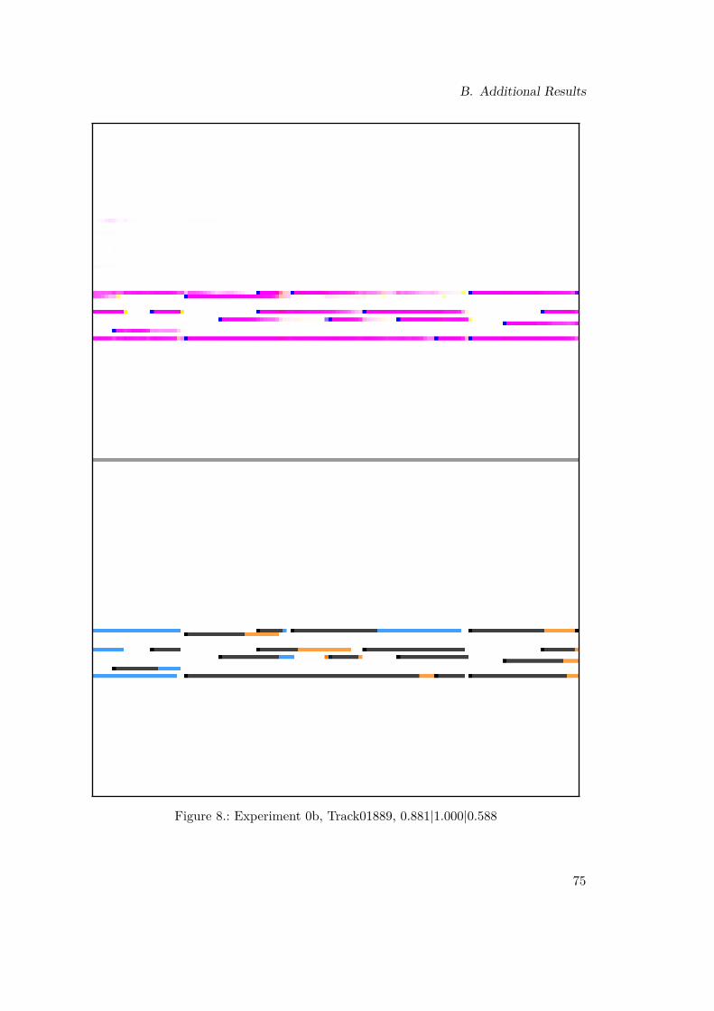
B. Additional Results

Figure 8.: Experiment 0b, Track01889, 0.881|1.000|0.588

75

Appendix

Figure 9.: Experiment 0c, Track01877, 0.755|0.900|0.717

76

B. Additional Results

Figure 10.: Experiment 0c, Track01892, 0.785|0.875|0.562

77

Appendix

Figure 11.: Experiment 0c, Track01893, 0.976|0.981|0.830

78

B. Additional Results

Figure 12.: Experiment 0c, Track01895, 1.000|1.000|1.000

79

Appendix

Figure 13.: Experiment 4a, Track01882, 0.657|0.692|0.538

80

B. Additional Results

Figure 14.: Experiment 4a, Track01892, 0.900|0.889|0.626

81

Appendix

Figure 15.: Experiment 4a, Track01932, 0.880|0.585|0.585

82

B. Additional Results

Figure 16.: Experiment 4a, Track01950, 0.894|0.886|0.514

83

Appendix

Figure 17.: Experiment 4a, Track01955, 0.682|0.750|0.714

84

B. Additional Results

Figure 18.: Experiment 4a, Track01956, 0.786|0.727|0.591

85

Appendix

Figure 19.: Experiment 4a, Track01957, 0.808|0.658|0.342

86

B. Additional Results

Figure 20.: Experiment 4a, Track01959, 0.000|0.000|0.000

87

Appendix

Figure 21.: Experiment 4a, Track01963, 0.588|0.913|0.261

88

NTN

UN

orw

egia

n U

nive

rsity

of S

cien

ce a

nd T

echn

olog

yFa

culty

of I

nfor

mat

ion

Tech

nolo

gy a

nd E

lect

rical

Eng

inee

ring

Dep

artm

ent o

f Com

pute

r Sci

ence

Henrik G

rønbechM

ulti-Instrument Autom

atic Music Transcription w

ith Deep Learning

Henrik Grønbech

Multi-Instrument Automatic MusicTranscription with Deep Learning

Master’s thesis in Computer ScienceSupervisor: Björn Gambäck

June 2021

Mas

ter’s

thes

is