1

MRI-based skeletal hand movement modelGeorg Stillfried, Ulrich Hillenbrand, Marcus Settles and Patrick van der Smagt

This paper is part of the book: Ravi Balasubra-manian and Veronica Santos (editors), The HumanHand as an Inspiration for Robot Hand Develop-ment. Springer Tracts in Advanced Robotics. 2014.URL: http://link.springer.com/book/10.1007/978-3-319-03017-3

Abstract—The kinematics of the human hand is optimalwith respect to force distribution during pinch as wellas power grasp, reducing the tissue strain when exertingforces through opposing fingers and optimising contactfaces. Quantifying this optimality is of key importancewhen constructing biomimetic robotic hands, but un-derstanding the exact human finger motion is also animportant asset in, e.g., tracking finger movement duringmanipulation. The goal of the method presented here isto determine the precise orientations and positions of theaxes of rotation of the finger joints by using suitablemagnetic resonance imaging (MRI) images of a handin various postures. The bones are segmented from theimages, and their poses are estimated with respect to areference posture. The axis orientations and positions arefitted numerically to match the measured bone motions.Eight joint types with varying degrees of freedom areinvestigated for each joint, and the joint type is selectedby setting a limit on the rotational and translationalmean discrepancy. The method results in hand modelswith differing accuracy and complexity, of which threeexamples, ranging from 22 to 33 DoF, are presented. Theranges of motion of the joints show some consensus andsome disagreement with data from literature. One of themodels is published as an implementation for the freeOpenSim simulation environment. The mean discrepanciesfrom a hand model built from MRI data are comparedagainst a hand model built from optical motion capturedata.

Index Terms—human hand, robot hand, hand kinemat-ics, MR imaging, 3D object localisation

G. Stillfried and U. Hillenbrand are with the Institute of Roboticsand Mechatronics, German Aerospace Center (DLR), Wessling, Ger-many. E-mail: {georg.stillfried,ulrich.hillenbrand}@dlr.de

P. v. d. Smagt is with the Faculty of Informatics, TechnischeUniversitat Munchen, Munich, Germany.

M. Settles is with Klinikum rechts der Isar, university hospital ofTU Munchen, Munich, Germany. E-mail: msettles@tum.de

Fig. 1. The joints and bones of the fingers, the thumb and themetacarpus that are investigated here. Bone contours adapted from[32].

FREQUENTLY USED ABBREVIATIONS

BonesMC metacarpal bonePP proximal phalanxPM medial phalanxPD distal phalanx

JointsCMC carpometacarpal jointIMC intermetacarpal jointMCP metacarpophalangeal jointPIP proximal interphalangeal jointDIP distal interphalangeal jointIP1 thumb interphalangeal joint

OtherDoF degree(s) of freedomLOOCV leave-one-out cross-validationMRI magnetic resonance imagingMoCap (optical) motion capture

The abbreviations for bones and joints are augmentedby numbers from 1 for thumb to 5 for little finger.For the location of the joints and bones, see Figure 1.Abbreviations for the joint types are found in Figure 6.

I. INTRODUCTION

Many robot hands have been built after the humanexample, one of the latest being the DLR Hand ArmSystem [1] (Figure 2). The design of its kinematicswas guided by simple length measurements of a humanhand, by functional considerations (e.g. how do the joint

2

Fig. 2. Hand, wrist and forearm of the DLR Hand Arm System [1].

axes need to be inclined in order to achieve a robustopposition grasp, Figure 3) and by intuitive appeal ofdifferent models to human subjects [2]. Each movementdegree of freedom (DoF) of the hand is supplementedby a stiffness DoF, so that 21 movement DoF of thehand and wrist are driven by 42 antagonistically placedmotors. By tensioning non-linear spring elements be-tween the motors and the joints, the mechanical stiffnesscan be adjusted. This allows to mimic humans’ stiffnessvariation in manipulation tasks, to store energy, e.g. forfinger flicking, and to survive heavy collisions. Withthe motors placed in the robotic “forearm”, the handis embedded in a Hand Arm System, which providesfive additional movement DoF for shoulder, elbow andforearm rotation.

Here we present a method that aims at very preciselymeasuring and modelling movement of the human handskeleton, in order to verify and further improve robothand kinematics. The method is demonstrated by creat-ing hand models that cover all joints of fingers and thumbas well as the palm arching movement of the metacarpus(Figure 1). The models are based on magnetic resonanceimaging (MRI) of an individual hand in 51 differentpostures, from which bone poses are extracted, localised,and used to optimise a parametrised general hand model.

Existing methods for modelling hand kinematics aremostly based on cadaver measurements [3]–[8] andoptical surface tracking [9]–[16].

In our opinion, measurements at hand cadavers can-not be used to reconstruct the active kinematics ofthe hands, since the muscle synergies cannot be takeninto account, plus the fixture by the ligaments is nolonger realistic; consequently, such models will lead toartefacts in the kinematic representation. Models basedon tracking the surface of the fingers, on the other hand,lead to unknown inaccuracies due to non-linear andvarying movement of the soft tissue (e.g., the skin) withrespect to the bones[17], [18]; indeed, such models oftenignore phalanx rotation around their longitudinal axis. Toovercome these disadvantages, we measure bone posesin vivo using 3D medical imaging. We conjecture that

Fig. 3. Human hand kinematics enables optimal grasps by aptlyorienting surfaces with respect to each other. Here the finger pads ofthumb and index finger are brought face-to-face.

our method therefore leads to more accurate models ofhuman hands.

The first and probably only previous work that usedMRI images for measuring finger kinematics is byMiyata et al. [19]. They recorded one reference postureand three other postures to determine helical movementaxes for the flexion axes of the proximal and distalinterphalangeal joints of the index finger (PIP2 andDIP2).

We aim to extend the MRI-based kinematic analysisin three ways:

1) covering all joints of the hand, including multi-DoF joints;

2) covering the range of motion of all the joints; and3) constructing a continuous representation of the

hand kinematics from which any intermediate pos-ture can be generated.

For solving these issues, we need to reproduciblymeasure the movement of fixed parts of the fingers, i.e.,the bones.

We model the human hand as a kinematic chainwith an arbitrary number of DoF per joint. The optimalnumber of DoF for each joint, as well as the staticparameters of each of these joints, are optimised fromthe recorded data. Once these parameters are determinedfor each of the joints, a model is generated with a fixednumber of DoF. Since the model is targeted towards thesubsequent implementation in a robotic system [20], onlyrotary joints are considered—any more complex joint ina robotic system will probably create friction and controldifficulties.

Data recording is focussed on single subjects ratherthan statistical averages. When reproducing the kinemat-ics of the human hand, statistics are of no great help: thatapproach would average over a number of participantswithout taking principal components of the variation intoaccount. Instead, the kinematics of one adult individualis measured and reproduced.

The resulting model is made available within theOpenSim simulation environment [21]. OpenSim is a

3

software that is able to match motion capture data toskeletal models, and can be extended to include tendonsand muscles. Much of the human skeleton is alreadycovered: legs, torso, neck, arms and a cadaver-basedthumb and index finger [22]. The hand model presentedhere will be a step towards the completion of the humanskeletal model.

II. METHODS

In order to determine the kinematics of the humanhand, the rigid bones—forming the endoskeletal struc-ture of the hand—are assumed as key reference pointsin the kinematics. The active kinematics is investigated,i.e., as induced by actively moving the joints throughmuscle activation, but passive kinematics, i.e., as inducedby putting external forces on the fingers of the hand,is ignored. The presented reconstruction of the activekinematics of the human hand is based on the followingscheme:

1) first, 3-dimensional MRI images of the hand arerecorded in a large number of predefined postures(Section II-A). The postures must be chosen soas to represent the full kinematic range of thehand. Among a large number of other postures,the Kapandji Test [23] for the assessment of thumbmotion is used;

2) second, in each 3-D MRI image the bones aresegmented, using automatic grey-level-based seg-mentation followed by manual correction;

3) third, the position and orientation of each of thebones of the hand is determined. This is doneautomatically using novel image-processing algo-rithms, in which statistical methods are used tolocalise known objects in a 3-dimensional visualscene (Section II-B);

4) finally, from a range of possible joint models(Section II-C), the optimal model for each jointis selected and the parameters of the joints aredetermined in order to minimise the errors in themodel (Section II-D). From that, kinematic chainsare defined for each of the fingers, thus ending upwith the full kinematic model.

The results of these steps are presented in Section III.

A. MRI images and segmentation

The MRI images are taken on a Philips Achieva 1.5 Tunit with a Philips SENSE eight-channel head coil toreceive a more homogeneous signal and to improve thesignal-to-noise ratio (SNR). Generally, SNR is propor-

tional to the voxel1 volume and to the square root of thenet scan duration:

r ∝ v√t, (1)

where r is the SNR, v is the voxel volume and t is thenet scan duration, i.e., the time actually spent for signalacquisition. Thus for every application an individualcompromise has to be found optimally balancing theneeds for a small v (high spatial resolution), small t(short scan times to minimise potential motion artefacts)and large r (image quality sufficient for either diag-nosis or—as in this case—the segmentation of certainanatomic structures).

An optimal compromise is found with a total scanduration (which is always longer than the net scanduration) of between two and two and a half minutesand a spatial resolution of (0.76 mm)3. Note that, fromEquation (1), a voxel volume of (0.38 mm)3 wouldrequire 64 times the scan duration in order to achievethe same SNR. To further minimise motion artefactsthe hand is stabilised using modelling clay. For post-processing, the spatial resolution is interpolated to (0.38mm)3 in order to achieve sub-voxel resolution in thesegmentation process. In the processing step after thesegmentation, the grey value information is discarded.The interpolation helps retain some of the informationthat is contained in the grey values.

For scanning, the sequence type balancedFFE isused (also known as trueFISP or balancedSSFP) withTR/TE/flip angle = 4.8 ms/2.4 ms/45°. The repetition timeTR is the time between two successive excitation pulses.The transverse component of the magnetization is readout at echo time TE after each pulse.

The advantage of balancedFFE is that it yields a strongsignal at short TR. (In fact, the signal of the balancedFFEsequence becomes independent of TR, which can be aslow as 2.5 ms with the limiting factors being the readouttime and the avoidance of peripheral and heart musclestimulation.)

As a drawback, balancedFFE is prone to the so-calledbanding artefacts appearing as black stripes across thebone. This artefact can in principle be overcome byapplying the balancedFFE offset averaging technique(also known as CISS or FIESTA-C), but requires twicethe scan time.

Another artefact occurring in these sequences is op-posed phase fat/water cancelling, where voxels contain-ing both fat and water, i.e. at corresponding tissue bound-aries, appear dark, because the magnetisation vectors offat and water point in opposite directions.

1voxel “volume pixel” = basic volume element of a 3-D image;analogous to pixel in 2-D images

4

Also a cine-sequence, i.e. a continuous-motion se-quence with two to five images per second, is recorded.However, only one image layer for the whole hand canbe recorded, which renders this method unusable for thepurpose of exact bone localisation.

The images are taken of a 29 year old female subjectwith no history of hand problems who gave informedconsent to the procedure. Fifty images are taken indifferent hand postures with the aim of reflecting eachjoint’s range of motion.

From the MRI volume images, the bones are seg-mented. In fact, not the whole bone volume is seg-mented but the signal-intense volume inside the bonethat corresponds to the cancellous bone. The tissuebetween the trabeculae of the cancellous bone is bonemarrow consisting mainly of fat, which yields high signalintensity in the balancedFFE sequence.

The cortical bone, which forms the outer calcifiedlayer of the bone, hardly contains any free fat or waterprotons and therefore stays dark in the MRI image.Near the bones there are other low-signal structureslike tendons, which makes it difficult to determine theouter bone surface. Therefore, the boundary betweencancellous and cortical bone is used for segmentation(Figure 4).

The bones are segmented from the image by high-lighting the cancellous bone area in each slice of theMRI image. In the medical imaging software Amira(Visage Imaging GmbH, Berlin, Germany), the area ispreselected by adjusting a threshold and refined manually(Figure 4).

B. Motion estimation

For the purpose of estimating the rigid motion ofbones between different hand postures, some geometricstructure rigidly related to each bone has to be extractedfrom the MRI images that can be reliably recoveredwith little shape variation between images. Automaticreconstruction of the bone geometry is a challenge, asthe image density of cancellous bone, cortical boneand surrounding tissue can vary greatly between andacross images. Also manual segmentation, besides beingtedious work, is prone to introducing shape variation.

Hence a double strategy is pursued. The border be-tween cancellous and cortical bone often produces amarked contrast edge at reproducible locations. Theseborder points can hence be detected by selection of high-contrast points. In the absence of such a marked densitycontrast, on the other hand, guidance by manual bonesegmentation is needed. This double strategy is imple-mented as follows. First, the bone segments are padded

Fig. 4. Segmentation process. Top left: Slice of an MRI image,showing the middle finger metacarpal (MC3). Tissue types canbe discriminated by the intensity of the signal that is emitted.Segmentation is done at the boundary between cancellous and corticalbone. Top right: Threshold-based preselection. Bottom left: Manuallyrefined selection. Bottom right: Segmented volume consisting of theselected areas from all slices.

with zero-density voxels to fit in a cuboid volume. Thena dipolarity score of the padded density within each3× 3× 3-voxel sub-volume is computed, as

Dipolarity(c1, c2, c3) =∥∥∥∥∥ ∑(i,j,k)∈{c1−1,c1+1}×{c2−1,c2+1}×{c3−1,c3+1}

I(i, j, k)

i− c1j − c2k − c3

∥∥∥∥∥.

Here I(i, j, k) is the MRI image density as function ofthe voxel indices (i, j, k), and (c1, c2, c3) are the indicesof the centre voxel within the considered 3×3×3-voxelsub-volume. The sum computes the density-weightedcentroid of voxels around the voxel at (c1, c2, c3); itsEuclidean norm quantifies the degree of dipolarity ofthe density at the centre voxel. It attains high values forcentre voxels close to a strong density edge. Finally, thecentre voxels with the top q percent of dipolarity areselected as representing bone-related points. The greyvalue information is discarded in the selected points,but the interpolation mentioned in section II-A is usedto refine the point set. The quantile q is chosen toproduce a data set of between 2,000 and 20,000 points,depending on the size of the bone. This way, points onthe manually determined bone border are selected in theabsence of high-contrast edges in the image; while high-contrast image edges dominate the selected points whereavailable.

5

The above procedure produces sets of points that areclose to the surface of the bones. However, missingparts and shape variation cannot be avoided. Moreover,there is no correspondence of points across different datasets of the same bone. A robust estimator of motionbetween such data sets hence has to be employed. Acorrespondence-free alignment that is also robust to ge-ometric deviations [24] is provided within the frameworkof parameter-density estimation and maximization, or pa-rameter clustering. This is a robust estimation techniquebased on location statistics in a parameter space whereparameter samples are computed from data samples [25],[26]. The estimator may be viewed as a continuousversion of a generalised, randomised Hough transform.In the present variant, samples are drawn from the 3-D points selected through the high-dipolarity criterionabove.

Let X,Y ⊂ R3 be the point sets extracted from twoMRI images of the same bone. A motion hypothesis canbe computed from a minimum subset of three pointsfrom X matched against a minimum subset of threepoints from Y . The sampling proceeds thus as follows:

1) Randomly draw a point triple x1, x2, x3 ∈ X;2) Randomly draw a point triple y1, y2, y3 ∈ Y that is

approximately congruent to the triple x1, x2, x3 ∈X;

3) Compute the rigid motion that aligns (x1, x2, x3)with (y1, y2, y3) in the least-squares sense;

4) Compute and store the six parameters of the hy-pothetical motion.

Random drawing of approximately congruent pointtriples in step 2 of the sampling procedure is efficientlyimplemented using a hash table of Y -point triples in-dexed with the three X-point distances (‖x1−x2‖, ‖x2−x3‖, ‖x3 − x1‖) as the key. Least-squares estimation ofrigid motion in step 3 computes the rotation R ∈ SO(3)and translation t ∈ R3 as

(R, t) = arg min(R′,t′)∈ SE(3)

[‖R′ x1 + t′ − y1‖2

+ ‖R′ x2 + t′ − y2‖2 + ‖R′x3 + t′ − y3‖2].

The special three-point method of [27] is used toobtain a closed-form solution. The parametrisation ofrigid motions chosen for sampling step 4 may have aninfluence on the result. In fact, the parameter densityfrom which the samples are taken depends upon thischoice. A parametrisation that is consistent for clusteringis used here, in the sense of [25].

By repeatedly executing the sampling procedure 1–4 above (in the order of 106 times), samples are ob-tained from the parameter density for the rigid alignment

problem. This parameter density is similar in spirit to aposterior density, but without assuming a probabilisticobservation model.

The parameter samples can be stored in an array ora tree of bins. The sampling stops when a significantcluster of samples has formed, as judged from the bincounts. Then the location of maximum parameter densityis searched by repeatedly starting a mean-shift procedure([28], [29]) from the centre of the bins with high param-eter counts. From all the local density maxima foundthrough mean shift, the location in the 6D parameterspace of the largest maximum is returned as the motionestimate of a bone, in the following denoted as Re andte. Details of the implementation are presented elsewhere[26].

The main sources of error in the procedure for esti-mating bone motion are

• the variation in bone geometry erroneously repre-sented in the point sets extracted from differentimages of the same bone, resulting from variation inmanual segmentation or dipolarity values computedfrom the images;

• the approximate rotational symmetry about the lon-gitudinal axis of a bone, especially in case of poorgeometric representation lacking shape details.

To get rid of grossly wrong motion estimates, aninteractive cluster analysis is performed on the es-timated rotations. Making use of the stochastic na-ture of the estimation algorithm, each motion esti-mate is repeated 100 times with different subsets ofthe data being sampled, resulting in motion estimates{Re1, te1} . . . {Re100, te100}. If the angular distance be-tween any two of the 100 motion estimates exceeds athreshold, clusters of rotation parameters are identifiedand the correct cluster C ⊂ {1, . . . , 100} is selectedthrough visual inspection (Figure 5).

The angular distance between two rotations is definedas the angle of a third rotation that would have tobe appended to the the first rotation in order to makeit identical to the second rotation. It is calculated asfollows:

angdist(R1, R2) := arccos

(1

2

(trace

(R2R

−11

)− 1))

,

(2)where R1 and R2 are the rotation matrices of the firstand second rotation.

The final rotation estimate R is determined as therotation that minimises the sum of squared angulardistances to all rotations in the cluster, i.e., the mean

6

Fig. 5. Visual inspection of pose estimates. The rotational part of100 randomly repeated pose estimates is plotted in three dimensionsas the product of rotation axis and angle. In this example there aretwo distinct clusters. One element in each cluster is inspected byregarding the more strongly curved side of the neighbouring bone(arrows). The motion of the bottom right cluster element impliesa large, anatomically impossible, longitudinal rotation of the bones.Therefore the top left cluster is taken as the correct cluster C.

rotation in the difference-rotation-angle metric,

R = argminR′ ∈ SO(3)

[∑i∈C

angdist(R′, Rei)2

], (3)

Likewise, the final translation estimate t is determinedas the translation that minimises the sum of squaredEuclidean distances to all translations in the cluster, i.e.,the ordinary mean value of valid translations,

t =1

n

∑i∈C

tcei, (4)

where n is the number of elements in the correct clusterC, and tcei is the i-th translation estimate of the bonecentroid. The translation estimate of the bone centroid iscalculated as follows:

tcei = Rei c + tei − c,

where c is the bone centroid, i.e. the mean of all points inX . If the correct cluster contains less than ten elements,the respective bone pose is discarded from the modellingprocess. Furthermore, all pose estimates are checkedoptically and obviously wrong estimates are discarded.

A natural confidence weight of the final rotationestimates is obtained from the variance of the samplemean values, i.e.,

σ2r =1

n(n− 1)

n∑i=1

angdist(R,Rei)2. (5)

This confidence weight enters in the estimation oforientation of rotational axes for the kinematic hand

Fig. 6. Joint types used in the presented method. From left to right:Hinge joint (one axis, “1a”), hinge joint with combined longitudinalrotation (two coupled intersecting axes, “2cia”), condyloid joint (twoorthogonal/oblique intersecting axes, “2oia”/“2ia”), saddle joint (twoorthogonal/oblique non-intersecting axes, “2ona”/“2na”), ball joint(three orthogonal intersecting axes, “3oia”) and 3-DoF joint withorthogonal non-intersecting axes (“3ona”, combination of a saddleand a pivot joint). Upper row images from [33].

model below. Likewise, a confidence weight of the finaltranslation estimates is given by

σ2t =1

n(n− 1)

n∑i=1

‖t− tcei‖2, (6)

and used in the estimation of the position of rotationalaxes for the kinematic hand model below.

C. Determining joint models

In the fingers of the human hand contain differenttypes of joints. The 1-DoF joints all are hinge joints(Figure 6); 2-DoF joints can be divided into two types.The metacarpal joint of the thumb is a saddle joint. Incontrast, the metacarpal joints of the fingers are condy-loid. The main difference between saddle and condyloidjoints is that condyloid joints have (roughly) intersectingaxes, which saddle joints do not have.

The condyloid and saddle joint types are furtherdivided into joints whose rotation axes are orthogonaland joints whose rotation axes are at any arbitrary angleto each other. Additionally, a hinge joint with a coupledlongitudinal rotation, a ball joint and a 3-DoF joint withnon-intersecting axes are defined (Figure 6).

As mentioned above, one of the goals is to compute anoptimal kinematic model for a robotic system. For thatreason, but also for reasons of computational efficiencyand easy representation, the joints are rotational jointswith axes fixed to the proximal bone or the precedingaxis in multi-DoF joints. This certainly has an effect onthe accuracy of the model, but this accuracy remainswithin the accuracy of the recording and reconstructionmethod.

Typically there is a trade-off between the complexityand the accuracy of a joint type. For each joint, the joint

7

type is selected by setting a limit on the mean deviationbetween the measured and modelled bone poses, andby selecting the simplest joint type that fulfils it. Jointsthat have fewer axes are considered simpler than jointswith more axes, intersecting axes simpler than non-intersecting axes and orthogonal axes simpler than freelyoriented ones. The mean deviation is an outcome of theidentification of the joint parameters (Section II-D).

D. Identification of joint parameters

The joint parameters (positions and orientations ofthe rotation axes) are identified on a joint-by-joint basisby numerically minimising the discrepancy between themeasured and modelled relative motion of the joint’s dis-tal bone with respect to the proximal bone. To calculatethe relative motion, the absolute motion of the proximalbone is inversely applied to the absolute motion of thedistal bone:

Rr = R−1p Rd (7)

and

tr = R−1p (cd + td − tp − cp) + cp − cd, (8)

where {Rr, tr} is the relative motion of the distal bonewith respect to the proximal bone, {Rp, tp} and {Rd, td}are the absolute motions of the proximal and distal boneaccording to Equations (3) and (4), and cp and cd arethe vectors of Cartesian coordinates of the centroids ofthe proximal and distal bone.

In order to reduce the dimensionality of the searchspace, the identification of the axis orientations andpositions is split up into two steps. In the first step, theaxis orientations are identified by minimising the angulardifference between the measured orientations and themodelled orientations.

The modelled orientation Rm of the bone is calculatedas follows:

Rm =

na∏k=1

rot(ak, qk) (9)

where na ∈ {1, 2, 3} is the number of rotation axesof the joint, ak is the orientation of the kth axis and qkis the rotation angle around the kth axis. The operatorrot(a, q) yields the rotation matrix of a rotation aroundan axis a by an angle q:

rot(a, q) := c+ c′ a2x c′ ax ay − az s c′ ax az + ay sc′ ax ay + az s c+ c′ a2y c′ ay az − ax sc′ ax az − ay s c′ ay az + ax s c+ c′ a2z

,

(10)

with

c = cos q,

c′ = 1− cos q and

s = sin q,

where ax, ay and az are the Cartesian elements of theunit orientation vector a. The position and orientationvectors of the rotation axes are given in the coordinatesystem of the MRI system, and with respect to the bonesin the reference posture.

The orientations of the rotation axes and the rota-tion angles are identified by numerically minimisingthe weighted mean square angular difference over allpostures:

(a1, . . . , ana, q1, . . . , qnp

) = argmin(a′

1,...,a′na

,q′1,...,q′

np) np∑

j=1

wrj angdist(Rrj , Rmj(a′1, . . . , a

′na, q′j)

)2 , (11)

with

wrj =1

σ2rpj + σ2rdj(12)

where np is the number of postures, a1, . . . , anaare

the orientation vectors of the rotation axes, q1, . . . , qnp

are the vectors of joint angles for each posture j ∈{1, . . . , np}, where qj = (q1j , . . . , qnaj)

T contains thejoint angles for each rotation axis, wrj is the confidenceweight due to the variances σ2rpj and σ2rdj of the rotationestimates of the proximal and distal bone in posture jas calculated in Equation (5), angdist is the angulardistance operator according to Equation (2), Rrj is themeasured relative orientation of the bone in posture jaccording to Equation (7) and Rmj is the modelledrelative orientation of the bone according to Equation(9).

The positions of the rotation axes are identified byminimising the mean squared distance between the mea-sured and modelled position of the bone centroid:

(p1, . . . , pna) =

argmin(p′

1,,...,p′na

)

np∑j=1

wtj

∥∥tmj(p′1, . . . , p′na)− trj

∥∥2 , (13)

with

tmj(p′1) =

(na∏k=1

rot(ak, qkj)

)(cd−p′1)+p′1− cd (14)

8

for joints with intersecting axes,

tmj(p′1, . . . , p′na) =

(na∏k=1

rot(ak, qkj)

)cd +(

na∑k=1

(k−1∏l=1

rot(al, qlj)−k∏

l=1

rot(al, qlj))

p′k

)− cd

(15)

for joints with non-intersecting axes and

wtj =1

σ2tpj + σ2tdj, (16)

where p1, . . . , pnaare the position vectors of the rotation

axes, tmj are the modelled translations of the bonecentroid, trj are the measured translations of the bonecentroid, ak and qkj are the rotation axes and angles asderived from Equation (11) and cd is the position vectorof the distal bone centroid.

In order to perform the optimisations described inEquations (11) and (13), the fminsearch function of theMatlab computation software is used, which implementsthe Nelder-Mead simplex algorithm [30]. The algorithmis called with broadly different starting points to in-crease the chance of finding the global optimum, andnot only a local optimum. For Equation (11), a nestedoptimisation is conducted, with an outer optimisation forthe axis orientations a1, . . . , ana

. Within each iterationstep of the outer optimisation, a number of np inneroptimisations are carried out to find the optimum jointangles q1, . . . , qnp

. For the outer optimisation, the axisorientations are parametrised by two spherical coordi-nates (azimuth and elevation), in order to reduce thesearch space by one dimension as compared to Cartesiancoordinates for axis orientation.

E. Leave-one-out cross-validation of joint parameters

In order to check to what extent the results apply tothe investigated hand in general as opposed to beingoverfit to the investigated postures, a leave-one-out cross-validation is performed. For this, the parameters of thejoints are identified np times, with np being the numberof measured bone poses, where in each round one of theposes is left out. The joint parameters (axis orientationsand positions) resulting from each identification are usedto move the bone as close as possible to the omitted pose.The rotational and translational discrepancy betweenthe modelled and measured bone pose is calculated,and the weighted mean of rotational and translationaldiscrepancies between the modelled and measured boneposes is calculated.

F. Comparison with optical motion capture

Kinematic hand models are built based on MRI dataand based on optical motion capture (MoCap) data. Theresidual rotational and translational discrepancies of bothmodels are compared.

Another subject is recruited for MRI and MoCapmeasurements, because the previous subject was notavailable anymore. Due to time constraints, only onereference posture and 19 other postures are recorded withMRI, using a turboFFE sequence and a spatial resolutionof (1 mm)3. For MoCap, a Vicon system (OMG plc,Oxford, UK) with seven 0.3-megapixels cameras is used.One finger is recorded at a time, with three retroreflectivemarkers per finger segment. One reference time sampleand nineteen representative other samples are selectedfrom the capture data. In the reference frame, bonecoordinate systems are attached manually to the markertriples of each segment. The motion of the finger segmentfrom the reference posture to the other postures isdetermined using the least-squares method by [27].

One joint instead of three joints is used to model thepalm, because the motion of the single metacarpal bonesis difficult to discriminate with MoCap. The same fifteenjoints for fingers and thumb as described above areused. The thumb CMC joint is modelled with two non-orthogonal, non-intersecting axes (2na), the MCP jointsare modelled with two orthogonal, intersecting axes(2oia) and the remaining joints are modelled with singleaxes (1a). The axis parameters and residual rotationaland translational discrepancies are modelled as describedabove.

Additionally, whole finger postures are matched withboth methods. For this, the joints are concatenated toform kinematic chains. The global pose and the jointangles are optimised to minimise the mean rotationaland translational discrepancies between the modelled andmeasured bone poses. For this, a weighting between therotational and translational discrepancy is decided. Onemillimetre of translational discrepancy is treated with thesame weight as one degree of rotational discrepancy.

The means of the residual discrepancies are tested witha two-tailed Student’s t-test for unpaired data, with asignificance threshold α = 5%, to find out if they arestatistically significantly different. We conjecture that theMRI method will lead to lower residuals than MoCap,because the measurements are not disturbed by softtissue artefacts. The null hypothesis is that the meanresiduals are equal.

III. RESULTS

The calculation steps described in the previous Meth-ods section lead to optimised joint parameters. By setting

9

a limit on the modelling error, the joint types for eachjoint are found (Section III-A). The modelling error iscomputed for each joint and checked by a leave-one-outcross-validation (Section III-B). The measurement erroris assessed by a repeatability test (Section III-C). As faras available, results are compared to data from literature(Section III-D). The software implementation of the handmodel is introduced (Section III-E).

A. Joint types

The main results of the presented method are move-ment models of the analysed human hand. Dependingon the desired accuracy in terms of discrepancy betweenmodelled and measured bone poses, hand models withdifferent complexity are generated. In Figure 7, differenthand models from simple (top) to complex (bottom) arepresented.

In the simple model, four joints are modelled as 2-DoFuniversal joints: thumb, index, ring and little finger MCP.The other joints are modelled as 1-DoF hinge joints.

The intermediately complex hand model (middle) dif-fers from the simple one by providing two DoF each toMCP3 and CMC1. The joint axes of MCP3 intersect,while the ones of CMC1 do not.

The most complex model (bottom) models CMC1 withthree non-intersecting axes, with the third one allow-ing a longitudinal rotation (pro-/supination) of MC1. Alongitudinal rotation is also enabled in DIP2 and PIP5,while PIP2 allows a combined longitudinal rotation andsidewards movement. The little finger DIP joint allowsa longitudinal rotation only in an extended position.Additional DoF for sidewards movement are found inDIP2, DIP3, DIP4 and IP1.

The weighted-mean rotational deviation per jointranges from 1.6° in IMC3 to 5.5° in IP1. The max-imum rotational deviation in a single hand posture is17.2° in CMC1. Weighted-mean translational deviationranges from 0.9 mm (PIP4) to 2.6 mm (CMC1), and themaximum translational deviation in a single hand postureis 7.2 mm, and also occurs in CMC1. The examples inFigure 8 are supposed to give a feel of these values.

B. Cross-validation of the results

For most joints, there is only a slight increase ofthe rotational and translational modelling error fromthe whole data mean error (columns 3 and 5) to theLOOCV mean error. For example, in the thumb MCPjoint, the mean angular when using all poses is 2.5°,and the mean angular error of the LOOCV is 2.9°. In thesame joint, the mean translational error is 1.2 mm whentaking into account all poses and 1.3 mm in the LOOCV

Fig. 7. Variants of the kinematic model at different accuracyconstraints, dorsal view (left) and radial view (right).Top: 22 DoF, rotational deviation < 9°, translational deviation <6 mm. Middle: 24 DoF, rotational deviation < 6°, translational devia-tion < 3 mm. Bottom: 33 DoF, rotational deviation < 3°, translationaldeviation < 2 mm. In joints with more than one axis, the first one ismarked “1”, the second one “2”, and, if existing, the third one “3”.

10

Fig. 8. Comparison of measured (bright) and modelled (dark) boneposes in several postures. Top left: Pose of the bone MC4 relativeto MC3 in posture 36. The rotational discrepancy is 1.6° and thetranslational discrepancy is 1.0 mm. The arrow is the rotation axis ofthe modelled IMC4 joint that connects MC3 and MC4. Top middle:DP1 relative to PP1 in posture 1. Discrepancy: 5.5°, 1.4 mm. IP1 joint.Top right: MC1 relative to MC2 in posture 29. Discrepancy: 17.2°,6.4 mm. CMC1 joint. Bottom left: MP4 relative to PP4. Discrepancy:2.6°, 0.9 mm. PIP4 joint. Bottom middle: MC1 relative to MC2 inposture 24. Discrepancy: 5.5°, 2.6 mm. Bottom right: MC1 relativeto MC2 in posture 35. Discrepancy: 5.1°, 7.2 mm.

analysis. This means that the results are generally validfor the investigated individual hand and do not dependon certain postures.

All differences for the translational error are within0.2 mm and all differences for the rotational error arewithin 1.0° except for the thumb interphalangeal joint,where the difference is 1.2° and the little finger metacar-pophalangeal joint, where it is 3.0°. In these exceptionalcases the joint parameters depend strongly on the se-lection of the subset of bone poses. This means thatthere are single extreme poses is the data that are notadequately represented by the other poses.

C. Motion estimation repeatability

The repeatability of the motion estimations is exam-ined by repeating it 100 times with randomly permutedpoint sets. The standard deviation of the rotation andtranslation estimate is given in Table I as the square rootof the variance described in Equations (5) and (6).

D. Comparison with results from literature

Comparing the range of motion (RoM) of the MCPjoints with the values provided by [31], in most pointsthe results agree, but some are different. [31] states that

1) the flexion RoM “falls short of 90° for the indexbut increases progressively with the other fingers”,

2) “active extension [...] can reach up to 30° or 40°”and

TABLE ISTANDARD DEVIATION OF THE MOTION ESTIMATION FOR THE

ROTATIONAL (σr) AND TRANSLATIONAL (σt) PART. THEMINIMUM, MAXIMUM AND MEAN OVER ALL IMAGES ARE GIVEN.

σr (°) σt (mm)

bone min max mean min max meanMC1 1.0 5.3 3.0 0.1 0.2 0.1PP1 1.6 5.7 3.2 0.1 0.3 0.1PD1 1.2 5.4 1.8 0.1 0.3 0.1

MC2 1.7 8.0 3.2 0.1 0.4 0.2PP2 1.0 5.9 2.8 0.1 0.2 0.1PM2 1.2 3.7 2.1 0.0 0.1 0.1PD2 3.2 4.9 3.9 0.0 0.1 0.1

MC3 1.1 23.7 2.6 0.1 0.5 0.2PP3 1.3 5.8 3.1 0.1 0.2 0.1PM3 1.0 2.9 1.7 0.0 0.1 0.1PD3 2.9 5.1 3.3 0.1 0.4 0.2

MC4 1.4 7.6 3.3 0.1 0.5 0.1PP4 0.9 8.9 3.4 0.1 0.2 0.1PM4 1.2 8.5 2.5 0.0 0.4 0.1PD4 2.1 4.3 2.9 0.1 0.2 0.1

MC5 1.4 11.2 3.6 0.1 0.4 0.1PP5 1.5 7.1 3.3 0.0 0.1 0.1PM5 1.0 4.3 2.8 0.0 0.1 0.1PD5 0.1 4.4 3.1 0.0 0.1 0.0

all 0.1 23.7 2.9 0.0 0.5 0.1

3) “the index finger has the greatest side-to-sidemovement”.

In the hand we used in our measurements, a smallerflexion RoM for the index finger (80°) is measured, whilethere is an increase towards in the little finger: middleand ring finger are similar with 86° and 84°, respectively,and the little finger has a flexion RoM of 95°. Theactive extension RoM is 30° (index), 33° (middle), 43°(ring) and 52° (little finger) and therefore higher thanthe ones in [31] for the ring and little finger. We agreethat, for the hand we investigated, index finger side-to-side movement is greater than that of the other fingerswith 59° (index), 43° (middle), 44° (ring) and 54° (littlefinger).

For the PIP and DIP joint, Kapandji states that1) the “range of flexion in the PIP joints is greater

than 90°” and2) in the DIP joints “slightly less than 90°”,3) the range “increases from the second to fifth fin-

ger” to 135° (PIP5) and4) to “a maximum of 90°” (DIP5);5) the range for PIP extension is zero and6) for active DIP extension zero or trivial.

Our measurements agree with points 1 and 2. An in-crease from second to fifth finger (points 3 and 4) is notobserved. Small PIP and DIP extension angles (up to

11

Fig. 9. Screenshot of the OpenSim application. Each DoF of theskeletal model can be moved by a slider.

22.5°) are measured.

E. OpenSim

The OpenSim model of the hand contains simplifiedbone geometries and the full set of joints. The joints canbe moved by sliders (Figure 9). The OpenSim frameworkalso provides for the extension of the model with tendonsand muscles [21]. The model is available for downloadas a zip-compressed file at http://www.robotic.dlr.de/human hand.

F. Dependence of results on starting points

The result of the parameter identification is in somejoints sensitive to the optimisation starting point and inothers not. For example, the parameters of the CMC1joint were optimised with three different starting pointsfor each of the two axis orientations and three differentstarting points for the axis offset. The results are slightlysensitive to the axis orientation starting points, with rota-tional error ranging from 2.95° to 3.18°. The variation ofthe axis offset starting point has no effect on the results.In other joints, for example the IP1 joint, the optimisationstarting points have no effect on the result.

G. MRI versus MoCap

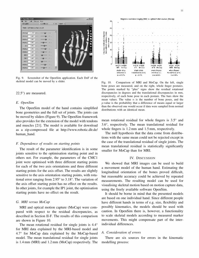
MRI and optical motion capture (MoCap) were com-pared with respect to the residual discrepancies, asdescribed in Section II-F. The results of this comparisonare shown in Figure 10.

The mean rotational residual for single joints is 4.4°for MRI data explained by the MRI-based model and4.7° for MoCap data explained by the MoCap-basedmodel. The mean translational residual for single jointsis 1.4 mm (MRI) and 1.2 mm (MoCap) respectively. The

Fig. 10. Comparison of MRI and MoCap. On the left, singlebone poses are measured, and on the right, whole finger postures.The points marked by “plus” signs show the residual rotationaldiscrepancies in degrees and the translational discrepancies in mm,respectively, of each bone pose in each posture. The bars show themean values. The value n is the number of bone poses, and thep-value is the probability that a difference of means equal or largerthan the observed one would occur if data were sampled from normaldistributions with an identical mean.

mean rotational residual for whole fingers is 3.5° and3.6°, respectively. The mean translational residual forwhole fingers is 1.2 mm and 1.5 mm, respectively.

The null hypothesis that the data come from distribu-tions with the same mean could not be rejected except inthe case of the translational residual of single joints. Themean translational residual is statistically significantlysmaller for MoCap than for MRI.

IV. DISCUSSION

We showed that MRI images can be used to builda movement model of the human hand. Estimating thelongitudinal orientation of the bones proved difficult,but reasonable accuracy could be achieved by repeatedmeasurements. The resulting model can be used forvisualising skeletal motion based on motion capture data,using the freely available software OpenSim.

It should be borne in mind that the presented modelsare based on one individual hand. Since different peoplehave different hands in terms of e.g. size, flexibility andpossibly kinematics, the models should be used withcaution. In OpenSim there is, however, a functionalityto scale skeletal models according to measured markermovements. This might compensate part of the inter-individual differences.

A. Consideration of errors

There are six sources for errors in the kinematicmodelling process:

12

Fig. 11. Histograms of the grey value distributions of middle fingermedial phalanx in different segmented MRI images. Three clearlydifferent examples are highlighted. Of these the central sagittal sliceof the MRI image is shown.

1) selection of postures,2) MRI acquisition,3) segmentation,4) motion estimation,5) joint definition, and6) joint parameter identification.

It is impossible to consider all possible postures of eachjoint as they are infinite. Ideal, therefore, would be avery dense sampling of postures during a large numberof different movements. This is not possible in MRIdue to cost and time constraints. Hand postures for thiswork are selected so that for each joint, the extremes andsome intermediate positions are covered. The selectionof postures influences the resulting model in the way thatmultiple recordings of similar joint postures assign thema greater weight compared to postures that occur onlyonce.

In MRI acquisition, same tissue can be representedby different grey values. Artefacts such as missing parts,motion artefacts, artefacts due to the surrounding tissueand possibly distortions can occur. A discretisation erroroccurs due to the spacial resolution of (0.76 mm)3.

In the segmentation process, the segmented shapedepends on the way the operator defines the grey valuethresholds and manually refines the selection. The com-bined error of MRI acquisition and segmentation is illus-trated by the distributions of grey value and segmentedvolume (Figures 11 and 12).

An attempt was made at measuring the error of theMRI image acquisition by taking images of an animalbone without surrounding tissue, in order to discard theneed for segmentation. However, the images showedhardly any signal, which might be due to the missingsurrounding tissue or to a lack of humidity within thebone.

The motion estimation error depends on the qualityof the segmented point clouds and the robustness of the

Fig. 12. Histogram of the segmented volumes of the middle fingermedial phalanx in different MRI images. Surface renderings of fourexamples are shown, with the image numbers and volumes in numberof voxels.

algorithm with respect to differences in shape and greyvalue distribution. The combined error of steps 2 to 4 ispartly expressed by the repeatability values in Table I,which however do not reflect a potential bias.

In this work, joints are modelled as rotational jointswith constant parameters. In the case of a 1-DoF joint,this corresponds to rigid joint surfaces with perfectlycircular cross-sections orthogonal to the joint axis. The3-DoF joint with intersecting axes would be ideallyrepresented by spherical joint surfaces. These are sim-plifications of the human joints with elastic cartilage andmore complex surfaces.

The parameters of the defined joints are identified byway of numerical optimisations. These may introduceerror by finding local optima. This error is assessed bythe robustness of the result in the face of varying startingpoints (Section III-F).

B. Joint types

The model in the middle of Figure 7 seems to bethe most natural one with two DoF for the thumb CMCand the MCP joints and one DoF for all other joints.The simpler model lacks a second DoF in the thumbCMC joint and in the middle finger MCP joint. On theother hand, the more complex model at the bottom hasmany additional DoF: in the thumb CMC and IP joint,in the PIP joints of index and little finger and in allthe DIP joints. The tendon structure of the hand makesit seem unlikely or impossible that these axes representindependently actuated DoF. They probably compensatebone pose measurement errors or deviations of the bonesfrom a perfectly circular path that really occur in thehand.

C. Thumb CMC joint

At the thumb CMC joint, the largest translationalerror occurs. This might be due to the fact that the

13

thumb metacarpal poses are determined with respectto the index finger metacarpal. However, the bone thatthe thumb metacarpal articulates with is the trapeziumbone, which is one of the carpal bones. Another possibleexplanation is that the motion of this joint is morecomplex, so that simple rotation axes are not sufficientto fully model it.

D. Comparison between MRI and optical motion cap-ture

Fitting a model with equal number of DoF to eitherMRI or optical motion capture (MoCap) data yielded nostatistically significant differences in the mean residualsin three of four comparisons, and one statistically sig-nificant difference in favour of MoCap (Figure 8). Thiscontradicts our initial hypothesis that MRI data can befitted with significantly smaller residuals. The effect ofthe soft tissue artefact on MoCap data seems not to beas strong as initially postulated.

ACKNOWLEDGEMENT

The authors would like to thank Karolina Stonawskafor the tedious work of segmenting the bones. Thisproject was partly funded by the EU project The HandEmbodied (FP7-ICT-248587).

GLOSSARY

a) axis of rotation: A line in space around whichsubsequent objects rotate; in this chapter, the pose ofthe axis of rotation with respect to its parent axis isconsidered to be constant.

b) degrees of freedom (DoF): The number of time-varying variables that, in combination with the jointparameters, define the posture of an articulated object.

c) hand: The palm and fingers, i.e. the metacarpalbones, the phalanx bones and the soft tissue that coversthem. Many other sources include the wrist as part of thehand. However, in this chapter the robotic perspective ischose, i.e. the hand is responsible for the contact with theenvironment and the arm, including wrist, is responsiblefor the pose of the hand.

d) in vivo: In the living body.e) joint: A set of constraints on the relative poses

between two bodies.f) joint parameters: The time-independent quan-

tities that define the space of possible postures of anarticulated object, e.g. the positions and orientations ofthe rotation axes.

g) kinematics: The study of motion without regard-ing the forces that cause it. Generally, the study of trans-lational and rotational poses, velocities and accelerations;in this chapter limited to poses.

h) magnetic resonance imaging (MRI): A three-dimensional medical imaging method that makes tissuesinside the human body (primarily fat and water) visible;it measures the reaction of the magnetic spins of hydro-gen nuclei to an alignment by a strong static magneticfield and a deflection by a weaker varying magnetic field.

i) optical motion capture: A method for measur-ing movements by tracking retro-reflective marker ballsattached to the surface of the subject or objects usingtriangulation between camera images of the marker balls.

j) pose: The position and orientation of an object;in three-dimensional space, the pose of a rigid object isdescribed by six independent variables.

k) posture: The set of poses of multiple rigid bod-ies that constitute an articulated object. “Hand posture”refers to the set of poses of the bones that constitute thehand, where the bones are idealised as rigid objects.

l) segmentation: Highlighting tissues of an organ inmedical images from e.g. magnetic resonance imaging toobtain the set of points that constitute the volume of theorgan.

REFERENCES

[1] M. Grebenstein, A. Albu-Schaffer, T. Bahls, M. Chalon,O. Eiberger, W. Friedl, R. Gruber, U. Hagn, R. Haslinger,H. Hoppner, S. Jorg, M. Nickl, A. Nothhelfer, F. Petit, J. Reill,N. Seitz, T. Wimbock, S. Wolf, T. Wusthoff, and G. Hirzinger,“The DLR hand arm system,” 2011 IEEE International Con-ference on Robotics and Automation, 2011.

[2] M. Grebenstein, M. Chalon, G. Hirzinger, and R. Siegwart, “Amethod for hand kinematics designers - 7 billion perfect hands,”in Proceedings of 1st International Conference on AppliedBionics and Biomechanics, 2010.

[3] Y. Youm, T. E. Gillespie, A. E. Flatt, and B. L. Sprague,“Kinematic investigation of normal MCP joint,” Journal ofBiomechanics, vol. 11, pp. 109–118, 1978.

[4] K. N. An, E. Y. Chao, I. W. P. Cooney, and R. L. Linscheid,“Normative model of human hand for biomechanical analysis,”Journal of Biomechanics, vol. 12, pp. 775–788, 1979.

[5] B. Buchholz, T. J. Armstrong, and S. A. Goldstein, “Anthropo-metric data for describing the kinematics of the human hands,”Ergonomics, vol. 35, no. 3, pp. 261–273, 1992.

[6] A. Hollister, W. L. Buford, L. M. Myers, D. J. Giurintano, andA. Novick, “The axes of rotation of the thumb carpometacarpaljoint,” Journal of Orthopaedic Research, vol. 10, pp. 454–460,1992.

[7] A. Hollister, D. J. Giurintano, W. L. Buford, L. M. Myers, andA. Novick, “The axes of rotation of the thumb interphalangealand metacarpophalangeal joints,” Clinical Orthopaedics andRelated Research, vol. 320, pp. 188–193, 1995.

[8] J. L. Sancho-Bru, A. Perez-Gonzalez, M. Vergara-Monedero,and D. Giurintano, “A 3-D dynamic model of human finger forstudying free movements,” Journal of Biomechanics, vol. 34,pp. 1491–1500, 2001.

[9] G. S. Rash, P. Belliappa, M. P. Wachowiak, N. N. Somia,and A. Gupta, “A demonstration of the validity of a 3-Dvideo motion analysis method for measuring finger flexion andextension,” Journal of Biomechanics, vol. 32(12), pp. 1337–1341, 1999.

14

[10] L.-C. Kuo, F.-C. Su, H.-Y. Chiu, and C.-Y. Yu, “Feasibilityof using a video-based motion analysis system for measuringthumb kinematics,” Journal of Biomechanics, vol. 35, pp. 1499–1506, 2002.

[11] X. Zhang, L. Sang-Wook, and P. Braido, “Determining fingersegmental centers of rotation in flexion-extension based on sur-face marker measurement,” Journal of Biomechanics, vol. 36,pp. 1097–1102, 2003.

[12] P. Cerveri, N. Lopomo, A. Pedotti, and G. Ferrigno, “Derivationof centers of rotation for wrist and fingers in a hand kinematicmodel: Methods and reliability results,” Annals of BiomedicalEngineering, vol. 33, pp. 402–412, 2005.

[13] L. Y. Chang and N. S. Pollard, “Constrained least-squaresoptimization for robust estimation of center of rotation,” Journalof Biomechanics, vol. 40, no. 6, pp. 1392 – 1400, 2007.

[14] ——, “Robust estimation of dominant axis of rotation,” Journalof Biomechanics, vol. 40, no. 12, pp. 2707 – 2715, 2007.

[15] ——, “Method for determining kinematic parameters of thein vivo thumb carpometaracpal joint,” IEEE Transactions onBiomedical Engineering, vol. 55(7), p. 1879ff, 2008.

[16] Dexmart, “Deliverable D1.1 kinematic model of the humanhand,” Dexmart, Tech. Rep., 2009.

[17] J. H. Ryu, N. Miyata, M. Kouchi, M. Mochimaru, and K. H.Lee, “Analysis of skin movement with respect to flexional bonemotion using mr images of a hand,” Journal of Biomechanics,vol. 39, pp. 844–852, 2006.

[18] K. Oberhofer, K. Mithraratne, N. Stott, and I. Anderson, “Errorpropagation from kinematic data to modeled muscle-tendonlengths during walking,” Journal of Biomechanics, vol. 42, pp.77–81, 2009.

[19] N. Miyata, M. Kouchi, M. Mochimaru, and T. Kurihaya, “Fingerjoint kinematics from MR images,” in IEEE/RSJ InternationalConference on Intelligent Robots and Systems, 2005.

[20] M. Grebenstein and P. van der Smagt, “Antagonism for a highlyanthropomorphic hand-arm system,” Advanced Robotics, vol.22(1), pp. 39–55, 2008.

[21] S. L. Delp, F. Anderson, S. Arnold, P. J. Loan, A. Habib,C. John, E. Guendelman, and D. Thelen, “OpenSim: Open-source software to create and analyze dynamic simulationsof movement,” IEEE Transactions on Biomedical Engineering,vol. 54, pp. 1940–1950, 2007.

[22] R. V. Gonzales, T. S. Buchanan, and S. L. Delp, “How musclearchitecture and moment arms affect wrist flexion-extensionmoments,” Journal of Biomechanics, vol. 30, pp. 705–712,1997.

[23] A. Kapandji, “Cotation clinique de l’opposition et de la contre-opposition du pouce [clinical test of opposition and counter-opposition of the thumb],” Annales de Chirurgie de la Main,vol. 5(1), pp. 67–73, 1986.

[24] U. Hillenbrand, “Non-parametric 3D shape warping,” in Pro-ceedings International Conference on Pattern Recognition(ICPR), 2010.

[25] ——, “Consistent parameter clustering: definition and analysis,”Pattern Recognition Letters, vol. 28, pp. 1112–1122, 2007.

[26] U. Hillenbrand and A. Fuchs, “An experimental study of fourvariants of pose clustering from dense range data,” pp. 1427 –1448, 2011. [Online]. Available: http://www.sciencedirect.com/science/article/pii/S1077314211001445

[27] B. K. Horn, “Closed-form solution of absolute orientation usingunit quaternions,” Journal of the Optical Society of America A,vol. 4(4), pp. 629–642, 1987.

[28] K. Fukunaga and L. D. Hostetler, “The estimation of a gradientof a density function, with applications in pattern recognition,”IEEE Transactions on Information Theory, vol. 21, pp. 32–40,1975.

[29] D. Comaniciu and P. Meer, “Mean shift: a robust approachtoward feature space analysis,” IEEE Transactions Pattern Anal-ysis and Machine Intelligence, vol. 24, pp. 603–619, 2002.

[30] J. A. Nelder and R. Mead, “A simplex method for functionminimization,” The Computer Journal, vol. 7, no. 4, pp. 308–313, 1965.

[31] A. Kapandji, The Physiology of the Joints. Edinburgh:Churchill Livingstone, 1998.

[32] Wikipedia, “Hand,” http://en.wikipedia.org/wiki/Hand, 2009.[33] ——, “Hinge joint,” http://en.wikipedia.org/wiki/Hinge joint,

2006.