IEEE TRANSACTIONS ON COMPUTATIONAL INTELLIGENCE AND AI IN GAMES 1

Monte Carlo Search Algorithm Discoveryfor One Player Games

Francis Maes, David Lupien St-Pierre and Damien Ernst

Abstract—Much current research in AI and games is beingdevoted to Monte Carlo search (MCS) algorithms. While thequest for a single unified MCS algorithm that would performwell on all problems is of major interest for AI, practitionersoften know in advance the problem they want to solve, andspend plenty of time exploiting this knowledge to customize theirMCS algorithm in a problem-driven way. We propose an MCSalgorithm discovery scheme to perform this in an automaticand reproducible way. We first introduce a grammar over MCSalgorithms that enables inducing a rich space of candidatealgorithms. Afterwards, we search in this space for the algorithmthat performs best on average for a given distribution of trainingproblems. We rely on multi-armed bandits to approximatelysolve this optimization problem. The experiments, generatedon three different domains, show that our approach enablesdiscovering algorithms that outperform several well-known MCSalgorithms such as Upper Confidence bounds applied to Treesand Nested Monte Carlo search. We also show that the discoveredalgorithms are generally quite robust with respect to changes inthe distribution over the training problems.

Index Terms—Monte-Carlo Search, Algorithm Selection,Grammar of Algorithms

I. INTRODUCTION

MONTE CARLO search (MCS) algorithms rely on ran-dom simulations to evaluate the quality of states or

actions in sequential decision making problems. Most of therecent progress in MCS algorithms has been obtained byintegrating smart procedures to select the simulations to beperformed. This has led to, among other things, the UpperConfidence bounds applied to Trees algorithm (UCT, [1]) thatwas popularized thanks to breakthrough results in computerGo [2]. This algorithm relies on a game tree to store simulationstatistics and uses this tree to bias the selection of futuresimulations. While UCT is one way to combine random sim-ulations with tree search techniques, many other approachesare possible. For example, the Nested Monte Carlo (NMC)search algorithm [3], which obtained excellent results in thelast General Game Playing competition1 [4], relies on nestedlevels of search and does not require storing a game tree.

How to best bias the choice of simulations is still anactive topic in MCS-related research. Both UCT and NMCare attempts to provide generic techniques that perform wellon a wide range of problems and that work with little or noprior knowledge. While working on such generic algorithmsis definitely relevant to AI, MCS algorithms are in practice

Francis Maes, David Lupien St-Pierre and Damien Ernst are at the Depart-ment of Electrical Engineering and Computer Science, University of Liege,Liege, Belgium.

E-mail: {francis.maes, dlspierre, dernst}@ulg.ac.be1http://games.stanford.edu

widely used in a totally different scenario, in which a signif-icant amount of prior knowledge is available about the gameor the sequential decision making problem to be solved.

People applying MCS techniques typically spend plenty oftime exploiting their knowledge of the target problem so asto design more efficient problem-tailored variants of MCS.Among the many ways to do this, one common practice isautomatic hyper-parameter tuning. By way of example, theparameter C > 0 of UCT is in nearly all applications tunedthrough a more or less automated trial and error procedure.While hyper-parameter tuning is a simple form of problem-driven algorithm selection, most of the advanced algorithmselection work is done by humans, i.e., by researchers thatmodify or invent new algorithms to take the specificities oftheir problem into account.

The comparison and development of new MCS algorithmsgiven a target problem is mostly a manual search processthat takes much human time and is error prone. Thanks tomodern computing power, automatic discovery is becominga credible approach for partly automating this process. Inorder to investigate this research direction, we focus on thesimplest case of (fully-observable) deterministic single-playergames. Our contribution is twofold. First, we introduce agrammar over algorithms that enables generating a rich spaceof MCS algorithms. It also describes several well-knownMCS algorithms, using a particularly compact and elegantdescription. Second, we propose a methodology based onmulti-armed bandits for identifying the best MCS algorithm inthis space, for a given distribution over training problems. Wetest our approach on three different domains. The results showthat it often enables discovering new variants of MCS thatsignificantly outperform generic algorithms such as UCT orNMC. We further show the good robustness properties of thediscovered algorithms by slightly changing the characteristicsof the problem.

This paper is structured as follows. Section II formalizesthe class of sequential decision making problems consideredin this paper and formalizes the corresponding MCS algo-rithm discovery problem. Section III describes our grammarover MCS algorithms and describes several well-known MCSalgorithms in terms of this grammar. Section IV formalizesthe search for a good MCS algorithm as a multi-armed banditproblem. We experimentally evaluate our approach on differentdomains in Section V. Finally, we discuss related work inSection VI and conclude in Section VII.

arX

iv:1

208.

4692

v3 [

cs.A

I] 1

8 D

ec 2

012

IEEE TRANSACTIONS ON COMPUTATIONAL INTELLIGENCE AND AI IN GAMES 2

II. PROBLEM STATEMENT

We consider the class of finite-horizon fully-observabledeterministic sequential decision-making problems. A problemP is a triple (x1, f, g) where x1 ∈ X is the initial state, fis the transition function, and g is the reward function. Thedynamics of a problem is described by

xt+1 = f(xt, ut) t = 1, 2, . . . , T, (1)

where for all t, the state xt is an element of the state space Xand the action ut is an element of the action space. We denoteby U the whole action space and by Ux ⊂ U the subset ofactions which are available in state x ∈ X . In the context ofone player games, xt denotes the current state of the game andUxt

are the legal moves in that state. We make no assumptionson the nature of X but assume that U is finite. We assume thatwhen starting from x1, the system enters a final state after Tsteps and we denote by F ⊂ X the set of these final states2.Final states x ∈ F are associated to rewards g(x) ∈ R thatshould be maximized.

A search algorithm A(·) is a stochastic algorithm thatexplores the possible sequences of actions to approximatelymaximize

A(P = (x1, f, g)) ' argmaxu1,...,uT

g(xT+1) , (2)

subject to xt+1 = f(xt, ut) and ut ∈ Uxt. In order to

fulfill this task, the algorithm is given a finite amount ofcomputational time, referred to as the budget. To facilitatereproducibility, we focus primarily in this paper on a budgetexpressed as the maximum number B > 0 of sequences(u1, . . . , uT ) that can be evaluated, or, equivalently, as thenumber of calls to the reward function g(·). Note, however,that it is trivial in our approach to replace this definition byother budget measures, as illustrated in one of our experimentsin which the budget is expressed as an amount of CPU time.

We express our prior knowledge as a distribution overproblems DP , from which we can sample any number oftraining problems P ∼ DP . The quality of a search algorithmAB(·) with budget B on this distribution is denoted byJBA (DP ) and is defined as the expected quality of solutionsfound on problems drawn from DP :

JBA (DP ) = EP∼DP{ExT+1∼AB(P ){g(xT+1)}} , (3)

where xT+1 ∼ AB(P ) denotes the final states returned byalgorithm A with budget B on problem P .

Given a class of candidate algorithms A and given the bud-get B, the algorithm discovery problem amounts to selectingan algorithm A∗ ∈ A of maximal quality:

A∗ = argmaxA∈A

JBA (DP ) . (4)

2In many problems, the time at which the game enters a final state is notfixed, but depends on the actions played so far. It should however be notedthat it is possible to make these problems fit this fixed finite time formalismby postponing artificially the end of the game until T . This can be done, forexample, by considering that when the game ends before T , a “pseudo finalstate” is reached from which, whatever the actions taken, the game will reachthe real final state in T .

The two main contributions of this paper are: (i) a grammarthat enables inducing a rich space A of candidate MCSalgorithms, and (ii) an efficient procedure to approximatelysolve Eq. 4.

III. A GRAMMAR FOR MONTE-CARLO SEARCHALGORITHMS

All MCS algorithms share some common underlying gen-eral principles: random simulations, look-ahead search, time-receding control, and bandit-based selection. The grammar thatwe introduce in this section aims at capturing these principlesin a pure and atomic way. We first give an overall view ofour approach, then present in detail the components of ourgrammar, and finally describe previously proposed algorithmsby using this grammar.

A. Overall view

We call search components the elements on which ourgrammar operates. Formally, a search component is a stochas-tic algorithm that, when given a partial sequence of ac-tions (u1, . . . , ut−1), generates one or multiple completions(ut, . . . , uT ) and evaluates them using the reward functiong(·). The search components are denoted by S ∈ S, where Sis the space of all possible search components.

Let S be a particular search component. We define thesearch algorithm AS ∈ A as the algorithm that, given theproblem P , executes S repeatedly with an empty partialsequence of actions (), until the computational budget isexhausted. The search algorithm AS then returns the sequenceof actions (u1, . . . , uT ) that led to the highest reward g(·).

In order to generate a rich class of search components—hence a rich class of search algorithms—in an inductiveway, we rely on search-component generators. Such gen-erators are functions Ψ : Θ → S that define a searchcomponent S = Ψ(θ) ∈ S when given a set of parametersθ ∈ Θ. Our grammar is composed of five search com-ponent generators that are defined in Section III-B: Ψ ∈{simulate, repeat, lookahead, step, select}. Four of thesesearch component generators are parametrized by sub-searchcomponents. For example, step and lookahead are functionsS → S . These functions can be nested recursively to generatemore and more evolved search components. We constructthe space of search algorithms A by performing this in asystematic way, as detailed in Section IV-A.

B. Search components

Figure 1 describes our five search component generators.Note that we distinguish between search component inputsand search component generator parameters. All our searchcomponents have the same two inputs: the sequence of alreadydecided actions (u1, . . . , ut−1) and the current state xt ∈ X .The parameters differ from one search component generatorto another. For example, simulate is parametrized by asimulation policy πsimu and repeat is parametrized by thenumber of repetitions N > 0 and by a sub-search component.We now give a detailed description of these search componentgenerators.

IEEE TRANSACTIONS ON COMPUTATIONAL INTELLIGENCE AND AI IN GAMES 3

Fig. 1. Search component generators

SIMULATE((u1, . . . , ut−1), xt)Param: πsimu ∈ Πsimu

for τ = t to T douτ ∼ πsimu(xτ )xτ+1 ← f(xτ , uτ )

end forYIELD((u1, . . . , uT ))

————————

REPEAT((u1, . . . , ut−1), xt)Param: N > 0, S ∈ Sfor i = 1 to N do

INVOKE(S, (u1, . . . , ut−1), xt)end for

————————

LOOKAHEAD((u1, . . . , ut−1), xt)Param: S ∈ Sfor ut ∈ Uxt

doxt+1 ← f(xt, ut)INVOKE(S, (u1, . . . , ut), xt+1)

end for

————————

STEP((u1, . . . , ut−1), xt)Param: S ∈ Sfor τ = t to T do

INVOKE(S, (u1, . . . , uτ−1), xτ )uτ ← u∗τxτ+1 ← f(xτ , uτ )

end for

————————

SELECT((u1, . . . , ut−1), xt)Param: πsel ∈ Πsel, S ∈ Sfor τ = t to T do . Select

uτ ∼ πsel(x)xτ+1 ← f(xτ , uτ )if n(xτ+1) = 0 then

breakend if

end fortleaf ← τ

INVOKE(S, (u1, . . . , utleaf), xtleaf+1) . Sub-search

for τ = tleaf to 1 do . Backpropagaten(xτ+1)← n(xτ+1) + 1n(xτ , uτ )← n(xτ , uτ ) + 1s(xτ , uτ )← s(xτ , uτ ) + r∗

end forn(x1)← n(x1) + 1

Simulate The simulate generator is parametrized by a policyπsimu ∈ Πsimu which is a stochastic mapping from states to

Fig. 2. Yield and invoke commandsRequire: g : F → R, the reward functionRequire: B > 0, the computational budget

Initialize global: numCalls← 0Initialize local: r∗ ← −∞Initialize local: (u∗1, . . . , u

∗T )← ∅

procedure YIELD((u1, . . . , uT ))r = g(x)if r > r∗ then

r∗ ← r(u∗1, . . . , u

∗T )← (u1, . . . , uT )

end ifnumCalls← numCalls+ 1if numCalls = B then

stop searchend if

end procedureprocedure INVOKE(S ∈ S, (u1, . . . , ut−1) ∈ U∗, xt ∈ X )

if t ≤ T thenS((u1, . . . , ut−1), xt)

elseyield (u1, . . . , uT )

end ifend procedure

actions: u ∼ πsimu(x). In order to generate the completion(ut, . . . , uT ), simulate(πsimu) repeatedly samples actions uτaccording to πsimu(xτ ) and performs transitions xτ+1 =f(xτ , uτ ) until reaching a final state. A default choice forthe simulation policy is the uniformly random policy, definedas

E{πrandom(x) = u} =

{1|Ux| if u ∈ Ux0 otherwise.

(5)

Once the completion (ut, . . . , uT ) is fulfilled, the whole se-quence (u1, . . . , uT ) is yielded. This operation is detailed inFigure 2 and proceeds as follows: (i) it computes the reward ofthe final state xT+1, (ii) if the reward is larger than the largestreward found previously, it replaces the best current solution,and (iii) if the budget B is exhausted, it stops the search.

Since algorithm AP repeats P until the budget is exhausted,the search algorithm Asimulate(πsimu) ∈ A is the algorithmthat samples B random trajectories (u1, . . . , uT ), evaluateseach of the final state rewards g(xT+1), and returns the bestfound final state. This simple random search algorithm issometimes called Iterative Sampling [5].

Note that, in the YIELD procedure, the variables relativeto the best current solution (r∗ and (u∗1, . . . , u

∗T )) are defined

locally for each search component, whereas the numCallscounter is global to the search algorithm. This means that ifS is a search component composed of different nested levelsof search (see the examples below), the best current solutionis kept in memory at each level of search.

Repeat Given a positive integer N > 0 and a searchcomponent S ∈ S, repeat(N,S) is the search componentthat repeats N times the search component S. For example,

IEEE TRANSACTIONS ON COMPUTATIONAL INTELLIGENCE AND AI IN GAMES 4

S = repeat(10, simulate(πsimu)) is the search componentthat draws 10 random simulations using πsimu. The corre-sponding search algorithm AS is again iterative sampling,since search algorithms repeat their search component until thebudget is exhausted. In Figure 1, we use the INVOKE operationeach time a search component calls a sub-search component.This operation is detailed in Figure 2 and ensures that no sub-search algorithm is called when a final state is reached, i.e.,when t = T + 1.

Look-ahead For each legal move ut ∈ Uxt, lookahead(S)

computes the successor state xt+1 = f(xt, ut) and runs thesub-search component S ∈ S starting from the sequence(u1, . . . , ut). For example, lookahead(simulate(πsimu))is the search component that, given the partial sequence(u1, . . . , ut−1), generates one random trajectory foreach legal next action ut ∈ Uxt

. Multiple-step look-ahead search strategies naturally write themselveswith nested calls to lookahead. As an example,lookahead(lookahead(lookahead(simulate(πsimu))))is a search component that runs one random trajectory perlegal combination of the three next actions (ut, ut+1, ut+2).

Step For each remaining time step τ ∈ [t, T ],step(S) runs the sub-search component S, extractsthe action uτ from (u∗1, . . . , u

∗T ) (the best currently

found action sequence, see Figure 2), and performstransition xτ+1 = f(xτ , uτ ). The search componentgenerator step enables implementing time receding searchmechanisms, e.g., step(repeat(100, simulate(πsimu)))is the search component that selects the actions(u1, . . . , uT ) one by one, using 100 random trajectoriesto select each action. As a more evolved example,step(lookahead(lookahead(repeat(10, simulation(πsimu))))) isa time receding strategy that performs 10 random simulationsfor each two first actions (ut, ut+1) to decide which actionut to select.

Select This search component generator implements mostof the behaviour of a Monte Carlo Tree Search (MCTS,[1]). It relies on a game tree, which is a non-uniform look-ahead tree with nodes corresponding to states and edgescorresponding to transitions. The role of this tree is twofold:it stores statistics on the outcomes of sub-searches and itis used to bias sub-searches towards promising sequences ofactions. A search component select(πsel, S) proceeds in threesteps: the selection step relies on the statistics stored in thegame tree to select a (typically small) sub-sequence of actions(ut, . . . , utleaf

), the sub-search step invokes the sub-searchcomponent S ∈ S starting from (u1, . . . , utleaf

), and thebackpropagation step updates the statistics to take into accountthe sub-search result.

We use the following notation to denote the informationstored by the look-ahead tree: n(x, u) is the number of timesthe action u was selected in state x, s(x, u) is the sum ofrewards that were obtained when running sub-search afterhaving selected action u in state x, and n(x) is the numberof times state x was selected: n(x) =

∑u∈Ux n(x, u). In

order to quantify the quality of a sub-search, we rely onthe reward of the best solution that was tried during that

sub-search: r∗ = max g(x). In the simplest case, when thesub-search component is S = simulate(πsimu), r∗ is thereward associated to the final state obtained by making therandom simulation with policy πsimu, as usual in MCTS.In order to select the first actions, selection relies on aselection policy πsel ∈ Πsel, which is a stochastic functionthat, when given all stored information related to state x(i.e., n(x), n(x, u), and s(x, u),∀u ∈ Ux), selects an actionu ∈ Ux. The selection policy has two contradictory goalsto pursue: exploration, trying new sequences of actions toincrease knowledge, and exploitation, using current knowledgeto bias computational efforts towards promising sequences ofactions. Such exploration/exploitation dilemmas are usuallyformalized as a multi-armed bandit problem, hence πsel istypically one of policies commonly found in the multi-armedbandit literature. The probably most well-known such policyis UCB-1 [6]:

πucb−1C (x) = argmax

u∈Ux

s(x, u)

n(x, u)+ C

√lnn(x)

n(x, u), (6)

where division by zero returns +∞ and where C > 0 is ahyper-parameter that enables the control of the exploration /exploitation tradeoff.

C. Description of previously proposed algorithms

Our grammar enables generating a large class of MCS al-gorithms, which includes several already proposed algorithms.We now overview these algorithms, which can be describedparticularly compactly and elegantly thanks to our grammar:• The simplest Monte Carlo algorithm in our class is Itera-

tive Sampling. This algorithm draws random simulationsuntil the computational time is elapsed and returns thebest solution found:

is = simulate(πsimu). (7)

• In general, iterative sampling is used during a certain timeto decide which action to select (or which move to play)at each step of the decision problem. The correspondingsearch component is

is′ = step(repeat(N, simulate(πsimu))), (8)

where N is the number of simulations performed for eachdecision step.

• The Reflexive Monte Carlo search algorithm introduced in[7] proposes using a Monte Carlo search of a given levelto improve the search of the upper level. The proposedalgorithm can be described as follows:

rmc(N1, N2) = step(repeat(N1,

step(repeat(N2, simulate(πsimu))))), (9)

where N1 and N2 are called the number of meta-gamesand the number of games, respectively.

• The Nested Monte Carlo (NMC) search algorithm [3] isa recursively defined algorithm generalizing the ideas ofReflexive Monte Carlo search. NMC can be described in

IEEE TRANSACTIONS ON COMPUTATIONAL INTELLIGENCE AND AI IN GAMES 5

a very natural way by our grammar. The basic search levell = 0 of NMC simply performs a random simulation:

nmc(0) = simulate(πrandom) . (10)

The level l > 0 of NMC relies on level l − 1 in thefollowing way:

nmc(l) = step(lookahead(nmc(l − 1))) . (11)

• Single-player MCTS [8]–[10] selects actions one afterthe other. In order to select one action, it relies on selectcombined with random simulations. The correspondingsearch component is thus

mcts(πsel, πsimu, N) = step(repeat(N,

select(πsel, simulate(πsimu)))) , (12)

where N is the number of iterations allocated to eachdecision step. UCT is one of the best known variantsof MCTS. It relies on the πucb−1

C selection policy andis generally used with a uniformly random simulationpolicy:

uct(C,N) = mcts(πucb−1C , πrandom, N) . (13)

• In the spirit of the work on nested Monte Carlo, the au-thors of [11] proposed the Meta MCTS approach, whichreplaces the simulation part of an upper-level MCTSalgorithm by a whole lower-level MCTS algorithm. Whilethey presented this approach in the context of two-playergames, we can describe its equivalent for one-playergames with our grammar:

metamcts(πsel, πsimu, N1, N2) =

step(repeat(N1, select(πsel,

mcts(πsel, πsimu, N2)) (14)

where N1 and N2 are the budgets for the higher-level andlower-level MCTS algorithms, respectively.

In addition to offering a framework for describing thesealready proposed algorithms, our grammar enables generatinga large number of new hybrid MCS variants. We give, in thenext section, a procedure to automatically identify the bestsuch variant for a given problem.

IV. BANDIT-BASED ALGORITHM DISCOVERY

We now move to the problem of solving Eq. 4, i.e., offinding, for a given problem, the best algorithm A fromamong a large class A of algorithms derived with the grammarpreviously defined. Solving this algorithm discovery problemexactly is impossible in the general case since the objectivefunction involves two infinite expectations: one over the prob-lems P ∼ DP and another over the outcomes of the algorithm.In order to approximately solve Eq. 4, we adopt the formalismof multi-armed bandits and proceed in two steps: we firstconstruct a finite set of candidate algorithms AD,Γ ⊂ A(Section IV-A), and then treat each of these algorithms as anarm and use a multi-armed bandit policy to select how toallocate computational time to the performance estimation of

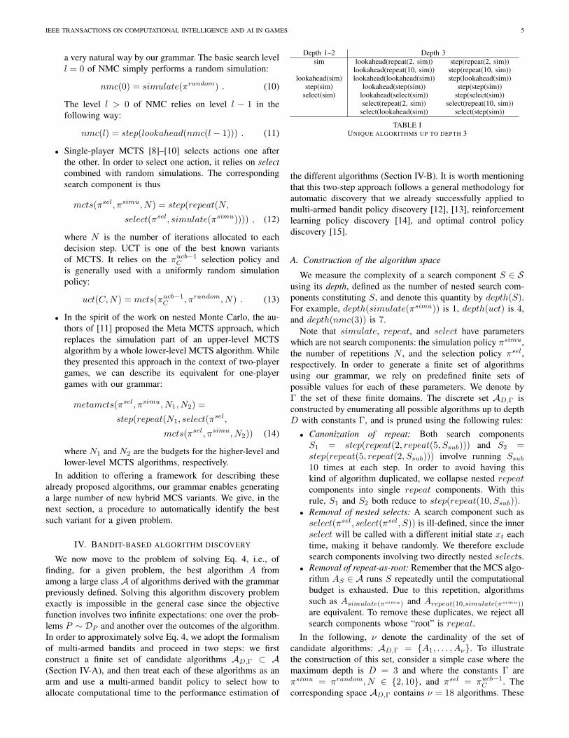
Depth 1–2 Depth 3sim lookahead(repeat(2, sim)) step(repeat(2, sim))

lookahead(repeat(10, sim)) step(repeat(10, sim))lookahead(sim) lookahead(lookahead(sim)) step(lookahead(sim))

step(sim) lookahead(step(sim)) step(step(sim))select(sim) lookahead(select(sim)) step(select(sim))

select(repeat(2, sim)) select(repeat(10, sim))select(lookahead(sim)) select(step(sim))

TABLE IUNIQUE ALGORITHMS UP TO DEPTH 3

the different algorithms (Section IV-B). It is worth mentioningthat this two-step approach follows a general methodology forautomatic discovery that we already successfully applied tomulti-armed bandit policy discovery [12], [13], reinforcementlearning policy discovery [14], and optimal control policydiscovery [15].

A. Construction of the algorithm space

We measure the complexity of a search component S ∈ Susing its depth, defined as the number of nested search com-ponents constituting S, and denote this quantity by depth(S).For example, depth(simulate(πsimu)) is 1, depth(uct) is 4,and depth(nmc(3)) is 7.

Note that simulate, repeat, and select have parameterswhich are not search components: the simulation policy πsimu,the number of repetitions N , and the selection policy πsel,respectively. In order to generate a finite set of algorithmsusing our grammar, we rely on predefined finite sets ofpossible values for each of these parameters. We denote byΓ the set of these finite domains. The discrete set AD,Γ isconstructed by enumerating all possible algorithms up to depthD with constants Γ, and is pruned using the following rules:• Canonization of repeat: Both search componentsS1 = step(repeat(2, repeat(5, Ssub))) and S2 =step(repeat(5, repeat(2, Ssub))) involve running Ssub10 times at each step. In order to avoid having thiskind of algorithm duplicated, we collapse nested repeatcomponents into single repeat components. With thisrule, S1 and S2 both reduce to step(repeat(10, Ssub)).

• Removal of nested selects: A search component such asselect(πsel, select(πsel, S)) is ill-defined, since the innerselect will be called with a different initial state xt eachtime, making it behave randomly. We therefore excludesearch components involving two directly nested selects.

• Removal of repeat-as-root: Remember that the MCS algo-rithm AS ∈ A runs S repeatedly until the computationalbudget is exhausted. Due to this repetition, algorithmssuch as Asimulate(πsimu) and Arepeat(10,simulate(πsimu))

are equivalent. To remove these duplicates, we reject allsearch components whose “root” is repeat.

In the following, ν denote the cardinality of the set ofcandidate algorithms: AD,Γ = {A1, . . . , Aν}. To illustratethe construction of this set, consider a simple case where themaximum depth is D = 3 and where the constants Γ areπsimu = πrandom, N ∈ {2, 10}, and πsel = πucb−1

C . Thecorresponding space AD,Γ contains ν = 18 algorithms. These

IEEE TRANSACTIONS ON COMPUTATIONAL INTELLIGENCE AND AI IN GAMES 6

algorithms are given in Table I, where we use sim as anabbreviation for simulate(πsimu).

B. Bandit-based algorithm discovery

One simple approach to approximately solve Eq. 4 is to es-timate the objective function through an empirical mean com-puted using a finite set of training problems {P (1), . . . , P (M)},drawn from DP :

JBA (DP ) ' 1

M

M∑i=1

g(xT+1)|xT+1 ∼ AB(P (i)) , (15)

where xT+1 denotes one outcome of algorithm A with budgetB on problem P (i). To solve Eq. 4, one can then computethis approximated objective function for all algorithms A ∈AD,Γ and simply return the algorithm with the highest score.While extremely simple to implement, such an approach oftenrequires an excessively large number of samples M to workwell, since the variance of g(·) may be quite large.

In order to optimize Eq. 4 in a smarter way, we proposeto formalize this problem as a multi-armed bandit problem.To each algorithm Ak ∈ AD,Γ, we associate an arm. Pullingthe arm k for the tkth time involves selecting the problemP (tk) and running the algorithm Ak once on this problem.This leads to a reward associated to arm k whose value is thereward g(xT+1) that comes with the solution xT+1 found byalgorithm Ak. The purpose of multi-armed bandit algorithmsis to process the sequence of observed rewards to select in asmart way the next algorithm to be tried, so that when the timeallocated to algorithm discovery is exhausted, one (or several)high-quality algorithm(s) can be identified. How to select armsso as to identify the best one in a finite amount of time isknown as the pure exploration multi-armed bandit problem[16]. It has been shown that index based policies based onupper confidence bounds such as UCB-1 were also goodpolicies for solving pure exploration bandit problems. Ouroptimization procedure works thus by repeatedly playing armsaccording to such a policy. In our experiments, we perform afixed number of such iterations. In practice this multi-armedbandit approach can provide an answer at anytime, returningthe algorithm Ak with the currently highest empirical rewardmean.

C. Discussion

Note that other approaches could be considered for solvingour algorithm discovery problem. In particular, optimizationover expression spaces induced by a grammar such as oursis often solved using Genetic Programming (GP) [17]. GPworks by evolving a population of solutions, which, in ourcase, would be MCS algorithms. At each iteration, the currentpopulation is evaluated, the less good solutions are removed,and the best solutions are used to construct new candidatesusing mutation and cross-over operations. Most existing GPalgorithms assume that the objective function is (at leastapproximately) deterministic. One major advantage of thebandit-based approach is to natively take into account thestochasticity of the objective function and its decomposability

into problems. Thanks to the bandit formulation, badly per-forming algorithms are quickly rejected and the computationalpower is more and more focused on the most promisingalgorithms.

The main strengths of our bandit-based approach are thefollowing. First, it is simple to implement and does not requireentering into the details of complex mutation and cross-over operators. Second, it has only one hyper-parameter (theexploration/exploitation coefficient). Finally, since it is basedon exhaustive search and on multi-armed bandit theory, formalguarantees can easily be derived to bound the regret, i.e., thedifference between the performance of the best algorithm andthe performance of the algorithm discovered [16], [18], [19].

Our approach is restricted to relatively small depths D sinceit relies on exhaustive search. In our case, we believe that manyinteresting MCS algorithms can be described using searchcomponents with low depth. In our experiments, we used D =5, which already provides many original hybrid algorithms thatdeserve further research. Note that GP algorithms do not sufferfrom such a limit, since they are able to generate deep andcomplex solutions through mutation and cross-over of smallersolutions. If the limit D = 5 was too restrictive, a major wayof improvement would thus consist in combining the idea ofbandits with those of GP. In this spirit, the authors of [20]recently proposed a hybrid approach in which the selection ofthe members of a new population is posed as a multi-armedbandit problem. This enables combining the best of the twoapproaches: multi-armed bandits enable taking natively intoaccount the stochasticity and decomposability of the objectivefunction, while GP cross-over and mutation operators are usedto generate new candidates dynamically in a smart way.

V. EXPERIMENTS

We now apply our automatic algorithm discovery approachto three different testbeds: Sudoku, Symbolic Regression, andMorpion Solitaire. The aim of our experiments was to showthat our approach discovers MCS algorithms that outper-form several generic (problem independent) MCS algorithms:outperforms them on the training instances, on new testinginstances, and even on instances drawn from distributionsdifferent from the original distribution used for the learning.

We first describe the experimental protocol in Section V-A.We perform a detailed study of the behavior of our approachapplied to the Sudoku domain in Section V-B. Section V-C,and V-D then give the results obtained on the other twodomains. Finally, Section V-E gives an overall discussion ofour results.

A. Protocol

We now describe the experimental protocol that will be usedin the remainder of this section.

Generic algorithms The generic algorithms are NestedMonte Carlo, Upper Confidence bounds applied to Trees,Look-ahead Search, and Iterative sampling. The search compo-nents for Nested Monte Carlo (nmc), UCT (uct), and Iterativesampling (is) have already been defined in Section III-C. The

IEEE TRANSACTIONS ON COMPUTATIONAL INTELLIGENCE AND AI IN GAMES 7

search component for Look-ahead Search of level l > 0 isdefined by la(l) = step(larec(l)), where

larec(l) =

{lookahead(larec(l − 1)) if l > 0

simulate(πrandom) otherwise.(16)

For both la(·) and nmc(·), we try all values within the range[1, 5] for the level parameter. Note that la(1) and nmc(1) areequivalent, since both are defined by the search componentstep(lookahead(simulate(πrandom))). For uct(·), we try thefollowing values of C: {0, 0.3, 0.5, 1.0} and set the budgetper step to B

T , where B is the total budget and T is thehorizon of the problem. This leads to the following set ofgeneric algorithms: {nmc(2), nmc(3), nmc(4), nmc(5), is,la(1), la(2), la(3), la(4), la(5), uct(0), uct(0.3), uct(0.5),and uct(1)}. Note that we omit the B

T parameter in uct forthe sake of conciseness.

Discovered algorithms In order to generate the set ofcandidate algorithms, we used the following constants Γ:repeat can be used with 2, 5, 10, or 100 repetitions; and selectrelies on the UCB1 selection policy from Eq. (6) with theconstants {0, 0.3, 0.5, 1.0}. We create a pool of algorithms byexhaustively generating all possible combinations of the searchcomponents up to depth D = 5. We apply the pruning rulesdescribed in Section IV-A, which results in a set of ν = 3, 155candidate MCS algorithms.

Algorithm discovery In order to carry out the algorithmdiscovery, we used a UCB policy for 100 × ν time steps,i.e., each candidate algorithm was executed 100 times onaverage. As discussed in Section IV-B, each bandit stepinvolves running one of the candidate algorithms on a problemP ∼ DP . We refer to DP as the training distribution in thefollowing. Once we have played the UCB policy for 100× νtime steps, we sort the algorithms by their average trainingperformance and report the ten best algorithms.

Evaluation Since algorithm discovery is a form of “learn-ing from examples”, care must be taken with overfittingissues. Indeed, the discovered algorithms may perform wellon the training problems P while performing poorly on otherproblems drawn from DP . Therefore, to evaluate the MCSalgorithms, we used a set of 10, 000 testing problems P ∼ DPwhich are different from the training problems. We thenevaluate the score of an algorithm as the mean performanceobtained when running it once on each testing problem.

In each domain, we futher test the algorithms either bychanging the budget B and/or by using a new distribution D′Pthat differs from the training distribution DP . In each suchexperiment, we draw 10, 000 problems from D′P and run thealgorithm once on each problem.

In one domain (Morpion Solitaire), we used a particularcase of our general setting, in which there was a singletraining problem P , i.e., the distribution DP was degenerateand always returned the same P . In this case, we focused ouranalysis on the robustness of the discovered algorithms whentested on a new problem P ′ and/or with a new budget B.

Presentation of the results For each domain, we present theresults in a table in which the algorithms have been sorted

according to their testing scores on DP . In each column ofthese tables, we underline both the best generic algorithmand the best discovered algorithm and show in bold allcases in which a discovered algorithm outperforms all testedgeneric algorithms. We furthermore performed an unpaired t-test between each discovered algorithm and the best genericalgorithm. We display significant results (p-value lower than0.05) by circumscribing them with stars. As in Table I, we usesim as an abbreviation for simulate(πsimu) in this section.

B. Sudoku

Sudoku, a Japanese term meaning “singular number”, is apopular puzzle played around the world. The Sudoku puzzleis made of a grid of G2 × G2 cells, which is structured intoblocks of size G×G. When starting the puzzle, some cells arealready filled in and the objective is to fill in the remainingcells with the numbers 1 through G2 so that• no row contains two instances of the same number,• no column contains two instances of the same number,• no block contains two instances of the same number.Sudoku is of particular interest in our case because each

Sudoku grid corresponds to a different initial state x1. Thus, agood algorithm A(·) is one that intrinsically has the versatilityto face a wide variety of Sudoku grids.

In our implementation, we maintain for each cell the listof numbers that could be put in that cell without violatingany of the three previous rules. If one of these lists becomesempty then the grid cannot be solved and we pass to a finalstate (see Footnote 2). Otherwise, we select the subset of cellswhose number-list has the lowest cardinality, and define oneaction u ∈ Ux per possible number in each of these cells (asin [3]). The reward associated to a final state is its proportionof filled cells, hence a reward of 1 is associated to a perfectlyfilled grid.

a) Algorithm discovery: We sample the initial states x1

by filling 33% randomly selected cells as proposed in [3]. Wedenote by Sudoku(G) the distribution over Sudoku problemsobtained with this procedure (in the case of G2×G2 games).Even though Sudoku is most usually played with G = 3 [21],we carry out the algorithm discovery with G = 4 to makethe problem more difficult. Our training distribution was thusDP = Sudoku(4) and we used a training budget of B = 1, 000evaluations. To evaluate the performance and robustness ofthe algorithms found, we tested the MCS algorithms on twodistributions: DP = Sudoku(4) and D′P = Sudoku(5), using abudget of B = 1, 000.

Table II presents the results, where the scores are theaverage number of filled cells, which is given by the rewardtimes the total number of cells G4. The best generic algorithmson Sudoku(4) are uct(0) and uct(0.3), with an average scoreof 198.7. We discover three algorithms that have a betteraverage score (198.8 and 198.9) than uct(0), but, due to avery large variance on this problem (some Sudoku grids are farmore easy than others), we could not show this difference to besignificant. Although the discovered algorithms are not signif-icantly better than uct(0), none of them is significantly worstthan this baseline. Furthermore, all ten discovered algorithms

IEEE TRANSACTIONS ON COMPUTATIONAL INTELLIGENCE AND AI IN GAMES 8

TABLE IIRANKING AND ROBUSTNESS OF ALGORITHMS DISCOVERED WHEN APPLIED TO SUDOKU

Name Search Component Rank Sudoku(4) Sudoku(5)Dis#8 step(select(repeat(select(sim, 0.5), 5), 0)) 1 198.9 487.2Dis#2 step(repeat(step(repeat(sim, 5)), 10)) 2 198.8 486.2Dis#6 step(step(repeat(select(sim, 0), 5))) 2 198.8 486.2uct(0) 4 198.7 494.4uct(0.3) 4 198.7 493.3Dis#7 lookahead(step(repeat(select(sim, 0.3), 5))) 6 198.6 486.4uct(0.5) 6 198.6 492.7Dis#1 select(step(repeat(select(sim, 1), 5)), 1) 6 198.6 485.7Dis#10 select(step(repeat(select(sim, 0.3), 5))) 9 198.5 485.9Dis#3 step(select(step(sim), 1)) 10 198.4 493.7Dis#4 step(step(step(select(sim, 0.5)))) 11 198.3 493.4Dis#5 select(step(repeat(sim, 5)), 0.5) 11 198.3 486.3Dis#9 lookahead(step(step(select(sim, 1)))) 13 198.1 492.8uct(1) 13 198.1 486.9nmc(3) 15 196.7 429.7la(1) 16 195.6 430.1nmc(4) 17 195.4 430.4nmc(2) 18 195.3 430.3nmc(5) 19 191.3 426.8la(2) 20 174.4 391.1la(4) 21 169.2 388.5is 22 169.1 388.5la(5) 23 168.3 386.9la(3) 24 167.1 389.1

—

TABLE IIIREPEATABILITY ANALYSIS

Search Component Structure Occurrences in the top-tenselect(step(repeat(select(sim)))) 11step(step(repeat(select(sim)))) 6step(select(repeat(select(sim)))) 5step(repeat(select(sim))) 5select(step(repeat(sim))) 2select(step(select(repeat(sim)))) 2step(select(step(select(sim)))) 2step(step(select(repeat(sim)))) 2step(repeat(step(repeat(sim)))) 2lookahead(step(repeat(select(sim)))) 2step(repeat(step(repeat(sim)))) 2select(repeat(step(repeat(sim)))) 1select(step(repeat(sim))) 1lookahead(step(step(select(sim)))) 1step(step(step(select(sim)))) 1step(step(step(repeat(sim)))) 1step(repeat(step(select(sim)))) 1step(repeat(step(step(sim)))) 1step(select(step(sim))) 1step(select(repeat(sim))) 1

—

are significantly better than all the other non-uct baselines.Interestingly, four out of the ten discovered algorithms rely onthe uct pattern – step(repeat(select(sim, ·), ·)) – as shownin bold in the table.

When running the algorithms on the Sudoku(5) games, thebest algorithm is still uct(0), with an average score of 494.4.This score is slightly above the score of the best discoveredalgorithm (493.7). However, all ten discovered algorithms arestill significantly better than the non-uct generic algorithms.This shows that good algorithms with Sudoku(4) are stillreasonably good for Sudoku(5).

b) Repeatability: In order to evaluate the stability of theresults produced by the bandit algorithm, we performed five

runs of algorithms discovery with different random seeds andcompared the resulting top-tens. What we observe is that ourspace contains a huge number of MCS algorithms performingnearly equivalently on our distribution of Sudoku problems. Inconsequence, different runs of the discovery algorithm producedifferent subsets of these nearly equivalent algorithms. Sincewe observed that small changes in the constants of repeatand select often have a negligible effect, we grouped thediscovered algorithms by structure, i.e. by ignoring the precisevalues of their constants. Table III reports the number ofoccurrences of each search component structure among thefive top-tens. We observe that uct was discovered in five casesout of fifty and that the uct pattern is part of 24 discoveredalgorithms.

c) Time-based budget: Since we expressed the budget asthe number of calls to the reward function g(·), algorithmsthat take more time to select their actions may be favored.To evaluate the extent of this potential bias, we performed anexperiment by setting the budget to a fixed amount of CPUtime. With our C++ implementation, on a 1.9 Ghz computer,about ≈ 350 Sudoku(4) random simulations can be performedper second. In order to have comparable results with thoseobtained previously, we thus set our budget to B = 1000

350 ≈ 2.8seconds, during both algorithm discovery and evaluation.

Table IV reports the results we obtain with a budgetexpressed as a fixed amount of CPU time. For each algorithm,we indicate also its rank in Table II. The new best genericalgorithm is now nmc(2) and eight out of the ten discoveredhave a better average score than this generic algorithm. Ingeneral, we observe that time-based budget favors nmc(·)algorithms and decreases the rank of uct(·) algorithms.

In order to better understand the differences between thealgorithms found with an evaluations-based budget and thosefound with a time-based budget, we counted the number of

IEEE TRANSACTIONS ON COMPUTATIONAL INTELLIGENCE AND AI IN GAMES 9

TABLE IVALGORITHMS DISCOVERED WHEN APPLIED TO SUDOKU WITH A CPU TIME BUDGET

Name Search Component Rank Rank in Table II Sudoku(4)Dis#1 select(step(select(step(sim), 0.3)), 0.3) 1 - 197.2Dis#2 step(repeat(step(step(sim)), 10)) 2 - 196.8Dis#4 lookahead(select(step(step(sim)), 0.3), 1) 3 - 196.1Dis#5 select(lookahead(step(step(sim)), 1), 0.3) 4 - 195.9Dis#3 lookahead(select(step(step(sim)), 0), 1) 5 - 195.8Dis#6 step(select(step(repeat(sim, 2)), 0.3)) 6 - 195.3Dis#9 select(step(step(repeat(sim, 2))), 0) 7 - 195.2Dis#8 step(step(repeat(sim, 2))) 8 - 194.8nmc(2) 9 18 194.7nmc(3) 10 15 194.5Dis#7 step(step(select(step(sim), 0))) 10 - 194.5Dis#10 step(repeat(step(step(sim)), 100)) 10 - 194.5la(1) 13 16 194.2nmc(4) 14 17 193.7nmc(5) 15 19 191.4uct(0.3) 16 4 189.7uct(0) 17 4 189.4uct(0.5) 18 6 188.9uct(1) 19 13 188.8la(2) 20 20 175.3la(3) 21 24 170.3la(4) 22 21 169.3la(5) 23 23 168.0is 24 22 167.8

—

occurrences of each of the search components among the tendiscovered algorithms in both cases. These counts are reportedin Table V. We observe that the time-based budget favorsthe step search component, while reducing the use of select.This can be explained by the fact that select is our searchcomponent that involves the most extra-computational cost,related to the storage and the manipulation of the game tree.

C. Real Valued Symbolic Regression

Symbolic Regression consists in searching in a large spaceof symbolic expressions for the one that best fits a givenregression dataset. Usually this problem is treated usingGenetic Programming approaches. In the line of [22], wehere consider MCS techniques as an interesting alternativeto Genetic Programming. In order to apply MCS techniques,we encode the expressions as sequences of symbols. Weadopt the Reverse Polish Notation (RPN) to avoid the useof parentheses. As an example, the sequence [a, b,+, c, ∗]encodes the expression (a+b)∗c. The alphabet of symbols weused is {x, 1,+,−, ∗, /, sin, cos, log, exp, stop}. The initialstate x1 is the empty RPN sequence. Each action u then addsone of these symbols to the sequence. When computing the setof valid actions Ux, we reject symbols that lead to invalid RPNsequences, such as [+,+,+]. A final state is reached eitherwhen the sequence length is equal to a predefined maximumT or when the symbol stop is played. In our experiments, weperformed the training with a maximal length of T = 11. Thereward associated to a final state is equal to 1−mae, wheremae is the mean absolute error associated to the expressionbuilt.

We used a synthetic benchmark, which is classical in thefield of Genetic Programming [23]. To each problem P of thisbenchmark is associated a target expression fP (·) ∈ R, and

TABLE VSEARCH COMPONENTS COMPOSITION ANALYSIS

Name Evaluations-based Budget Time-based Budgetrepeat 8 5simulate 10 10select 12 8step 16 23lookahead 2 3

—

TABLE VISYMBOLIC REGRESSION TESTBED: TARGET EXPRESSIONS AND DOMAINS.

Target Expression fP (·) Domainx3 + x2 + x [−1, 1]x4 + x3 + x2 + x [−1, 1]x5 + x4 + x3 + x2 + x [−1, 1]x6 + x5 + x4 + x3 + x2 + x [−1, 1]sin(x2) cos(x)− 1 [−1, 1]sin(x) + sin(x+ x2) [−1, 1]log(x+ 1) + log(x2 + 1) [0, 2]√x [0, 4]

—

the aim is to re-discover this target expression given a finiteset of samples (x, fP (x)). Table VI illustrates these targetexpressions. In each case, we used 20 samples (x, fP (x)),where x was obtained by taking uniformly spaced elementsfrom the indicated domains. The training distribution DP wasthe uniform distribution over the eight problems given in TableVI.

The training budget was B = 10, 000. We evaluate therobustness of the algorithms found in three different ways: bychanging the maximal length T from 11 to 21, by increasingthe budget B from 10,000 to 100,000 and by testing them onanother distribution of problems D′P . The distribution D′P is

IEEE TRANSACTIONS ON COMPUTATIONAL INTELLIGENCE AND AI IN GAMES 10

TABLE VIIIRANKING AND ROBUSTNESS OF THE ALGORITHMS DISCOVERED WHEN APPLIED TO SYMBOLIC REGRESSION

Name Search Component Rank T = 11 T = 21 T = 11, B = 105 D′P

Dis#1 step(step(lookahead(lookahead(sim)))) 1 *0.066* *0.083* *0.036* 0.101Dis#5 step(repeat(lookahead(lookahead(sim)), 2)) 2 *0.069* *0.085* *0.037* 0.106Dis#2 step(lookahead(lookahead(repeat(sim, 2)))) 2 *0.069* *0.084* *0.038* 0.100Dis#8 step(lookahead(repeat(lookahead(sim), 2))) 2 *0.069* *0.084* *0.040* 0.112Dis#7 step(lookahead(lookahead(select(sim, 1)))) 5 *0.070* 0.087 *0.040* 0.103Dis#6 step(lookahead(lookahead(select(sim, 0)))) 6 0.071 0.087 *0.039* 0.110Dis#4 step(lookahead(select(lookahead(sim), 0))) 6 0.071 0.087 *0.038* 0.101Dis#3 step(lookahead(lookahead(sim))) 6 0.071 0.086 0.056 0.100la(2) 6 0.071 0.086 0.056 0.100Dis#10 step(lookahead(select(lookahead(sim), 0.3))) 10 0.072 0.088 *0.040* 0.108la(3) 11 0.073 0.090 0.053 0.101Dis#9 step(repeat(select(lookahead(sim), 0.3), 5)) 12 0.077 0.091 *0.048* *0.099*nmc(2) 13 0.081 0.103 0.054 0.109nmc(3) 14 0.084 0.104 0.053 0.118la(4) 15 0.088 0.116 0.057 0.101nmc(4) 16 0.094 0.108 0.059 0.141la(1) 17 0.098 0.116 0.066 0.119la(5) 18 0.099 0.124 0.058 0.101is 19 0.119 0.144 0.087 0.139nmc(5) 20 0.120 0.124 0.069 0.140uct(0) 21 0.159 0.135 0.124 0.185uct(1) 22 0.147 0.118 0.118 0.161uct(0.3) 23 0.156 0.112 0.135 0.177uct(0.5) 24 0.153 0.111 0.124 0.184

—

TABLE VIISYMBOLIC REGRESSION ROBUSTNESS TESTBED: TARGET EXPRESSIONS

AND DOMAINS.

Target Expression fP (·) Domainx3 − x2 − x [−1, 1]x4 − x3 − x2 − x [−1, 1]x4 + sin(x) [−1, 1]cos(x3) + sin(x+ 1) [−1, 1]√

(x) + x2 [0, 4]x6 + 1 [−1, 1]sin(x3 + x2) [−1, 1]log(x3 + 1) + x [0, 2]

—

the uniform distribution over the eight new problems given inTable VII.

The results are shown in Table VIII, where we reportdirectly the mae scores (lower is better). The best genericalgorithm is la(2) and corresponds to one of the discoveredalgorithms (Dis#3). Five of the discovered algorithms signif-icantly outperform this baseline with scores down to 0.066.Except one of them, all discovered algorithms rely on twonested lookahead components and generalize in some waythe la(2) algorithm.

When setting the maximal length to T = 21, the bestgeneric algorithm is again la(2) and we have four discov-ered algorithms that still significantly outperform it. Whenincreasing the testing budget to B = 100, 000, nine discoveredalgorithms out of the ten significantly outperform the bestgeneric algorithms, la(3) and nmc(3). These results thus showthat the algorithms discovered by our approach are robust bothw.r.t. the maximal length T and the budget B.

In our last experiment with the distribution D′P , there isa single discovered algorithm that significantly outperformla(2). However, all ten algorithms behave still reasonably

well and significantly better than the non-lookahead genericalgorithms. This result is particularly interesting since it showsthat our approach was able to discover algorithms that workwell for symbolic regression in general, not only for someparticular problems.

D. Morpion SolitaireThe classic game of morpion solitaire [24] is a single

player, pencil and paper game, whose world record has beenimproved several times over the past few years using MCStechniques [3], [7], [25]. This game is illustrated in Figure 3.The initial state x1 is an empty cross of points drawn on theintersections of the grid. Each action places a new point at agrid intersection in such a way that it forms a new line segmentconnecting consecutive points that include the new one. Newlines can be drawn horizontally, vertically, and diagonally. Thegame is over when no further actions can be taken. The goalof the game is to maximize the number of lines drawn beforethe game ends, hence the reward associated to final states isthis number3.

There exist two variants of the game: “Disjoint” and“Touching”. “Touching” allows parallel lines to share anendpoint, whereas “Disjoint” does not. Line segments withdifferent directions are always permitted to share points. Thegame is NP-hard [26] and presumed to be infinite under certainconfigurations. In this paper, we treat the 5D and 5T versionsof the game, where 5 is the number of consecutive points toform a line, D means disjoint, and T means touching.

We performed the algorithm discovery in a “single trainingproblem” scenario: the training distribution DP always returns

3In practice, we normalize this reward by dividing it by 100 to make itapproximately fit into the range [0, 1]. Thanks to this normalization, we cankeep using the same constants for both the UCB policy used in the algorithmdiscovery and the UCB policy used in select.

IEEE TRANSACTIONS ON COMPUTATIONAL INTELLIGENCE AND AI IN GAMES 11

Fig. 3. A random policy that plays the game Morpion Solitaire 5T: initial grid; after 1 move; after 10 moves; game end.

the same problem P , corresponding to the 5T version of thegame. The initial state of P was the one given in the leftmostpart of Figure 3. The training budget was set to B = 10, 000.To evaluate the robustness of the algorithms, we, on the onehand, evaluated them on the 5D variant of the problem and,on the other hand, changed the evaluation budget from 10,000to 100,000. The former provides a partial answer to how rule-dependent these algorithms are, while the latter gives insightinto the impact of the budget on the algorithms’ ranking.

The results of our experiments on Morpion Solitaire aregiven in Table IX. Our approach proves to be particularly suc-cessful on this domain: each of the ten discovered algorithmssignificantly outperforms all tested generic algorithm. Amongthe generic algorithms, la(1) gave the best results (90.63),which is 0.46 below the worst of the ten discovered algorithms.

When moving to the 5D rules, we observe that all tendiscovered algorithms still significantly outperform the bestgeneric algorithm. This is particularly impressive, since it isknown that the structure of good solutions strongly differsbetween the 5D and 5T versions of the game [24]. The lastcolumn of Table IX gives the performance of the algorithmswith budget B = 105. We observe that all ten discovered algo-rithms also significantly outperform the best generic algorithmin this case. Furthermore, the increase in the budget seems toalso increase the gap between the discovered and the genericalgorithms.

E. Discussion

We have seen that on each of our three testbeds, we dis-covered algorithms, which are competitive with, or even sig-nificantly better than generic ones. This demonstrates that ourapproach is able to generate new MCS algorithms specificallytailored to the given class of problems. We have performed astudy of the robustness of these algorithms by either changingthe problem distribution or by varying the budget B, andfound that the algorithms discovered can outperform genericalgorithms even on problems significantly different from thoseused for the training.

The importance of each component of the grammar dependsheavily on the problem. For instance, in Symbolic Regres-sion, all ten best algorithms discovered rely on two nested

lookahead components, whereas in Sudoku and Morpion,step and select appear in the majority of the best algorithmsdiscovered.

VI. RELATED WORK

Methods for automatically discovering MCS algorithms canbe characterized through three main components: the space ofcandidate algorithms, the performance criterion, and the searchmethod for finding the best element in the space of candidatealgorithms.

Usually, researchers consider spaces of candidate algorithmsthat only differ in the values of their constants. In such acontext, the problem amounts to tuning the constants of ageneric MCS algorithm. Most of the research related to thetuning of these constants takes as performance criterion themean score of the algorithm over the distribution of targetproblems. Many search algorithms have been proposed forcomputing the best constants. For instance, [27] employs a gridsearch approach combined with self-playing, [28] uses cross-entropy as a search method to tune an agent playing GO, [29]presents a generic black-box optimization method based onlocal quadratic regression, [30] uses Estimation DistributionAlgorithms with Gaussian distributions, [31] uses ThompsonSampling, and [32] uses, as in the present paper, a multi-armedbandit approach. The paper [33] studies the influence of thetuning of MCS algorithms on their asymptotic consistency andshows that pathological behaviour may occur with tuning. Italso proposes a tuning method to avoid such behaviour.

Research papers that have reported empirical evaluationsof several MCS algorithms in order to find the best one arealso related to this automatic discovery problem. The spaceof candidate algorithms in such cases is the set of algorithmsthey compare, and the search method is an exhaustive searchprocedure. As a few examples, [27] reports on a comparisonbetween algorithms that differ in their selection policy, [34]and [35] compare improvements of the UCT algorithm (RAVEand progressive bias) with the original one on the game of GO,and [36] evaluates different versions of a two-player MCSalgorithm on generic sparse bandit problems. [37] providesan in-depth review of different MCS algorithms and theirsuccesses in different applications.

IEEE TRANSACTIONS ON COMPUTATIONAL INTELLIGENCE AND AI IN GAMES 12

TABLE IXRANKING AND ROBUSTNESS OF ALGORITHMS DISCOVERED WHEN APPLIED TO MORPION

Name Search Component Rank 5T 5D 5T,B = 105

Dis#1 step(select(step(simulate),0.5)) 1 *91.24* *63.66* *97.28*Dis#4 step(select(step(select(sim,0.5)),0)) 2 *91.23* *63.64* *96.12*Dis#3 step(select(step(select(sim,1.0)),0)) 3 *91.22* *63.63* *96.02*Dis#2 step(step(select(sim,0))) 4 *91.18* *63.63* *96.78*Dis#8 step(select(step(step(sim)),1)) 5 *91.12* *63.63* *96.67*Dis#9 step(select(step(select(sim,0)),0.3)) 6 *91.22* *63.67* *96.02*Dis#5 select(step(select(step(sim),1.0)),0) 7 *91.16* *63.65* *95.79*Dis#10 step(select(step(select(sim,1.0)),0.0)) 8 *91.21* *63.62* *95.99*Dis#6 lookahead(step(step(sim))) 9 *91.15* *63.68* *96.41*Dis#7 lookahead(step(step(select(sim, 0)))) 10 *91.08* 63.67 *96.31*la(1) 11 90.63 63.41 95.09nmc(3) 12 90.61 63.44 95.59nmc(2) 13 90.58 63.47 94.98nmc(4) 14 90.57 63.43 95.24nmc(5) 15 90.53 63.42 95.17uct(0) 16 89.40 63.02 92.65uct(0.5) 17 89.19 62.91 92.21uct(1) 18 89.11 63.12 92.83uct(0.3) 19 88.99 63.03 92.32la(2) 20 85.99 62.67 94.54la(3) 21 85.29 61.52 89.56is 21 85.28 61.40 88.83la(4) 23 85.27 61.53 88.12mcts 24 85.26 61.48 89.46la(5) 25 85.12 61.52 87.69

—

The main feature of the approach proposed in the presentpaper is that it builds the space of candidate algorithms byusing a rich grammar over the search components. In thissense, [38], [39] are certainly the papers which are the closestto ours, since they also use a grammar to define a search space,for, respectively, two player games and multi-armed banditproblems. However, in both cases, this grammar only modelsa selection policy and is made of classic functions such as +,−, ∗, /, log , exp , and √. We have taken one step forward,by directly defining a grammar over the MCS algorithms thatcovers very different MCS techniques. Note that the searchtechnique of [38] is based on genetic programming.

The decision as to what to use as the performance criterionis not as trivial as it looks, especially for multi-player games,where opponent modelling is crucial for improving over game-theoretically optimal play [40]. For example, the maximizationof the victory rate or loss minimization against a wide varietyof opponents for a specific game can lead to different choicesof algorithms. Other examples of criteria to discriminatebetween algorithms are simple regret [32] and the expectedperformance over a distribution density [41].

VII. CONCLUSION

In this paper we have addressed the problem of automati-cally identifying new Monte Carlo search (MCS) algorithmsperforming well on a distribution of training problems. To doso, we introduced a grammar over the MCS algorithms thatgenerates a rich space of candidate algorithms (and whichdescribes, along the way, using a particularly compact andelegant description, several well-known MCS algorithms). Toefficiently search inside this space of candidate algorithmsfor the one(s) having the best average performance on the

training problems, we relied on a multi-armed bandit type ofoptimisation algorithm.

Our approach was tested on three different domains: Su-doku, Morpion Solitaire, and Symbolic Regression. The re-sults showed that the algorithms discovered this way oftensignificantly outperform generic algorithms such as UCT orNMC. Moreover, we showed that they had good robustnessproperties, by changing the testing budget and/or by usinga testing problem distribution different from the trainingdistribution.

This work can be extended in several ways. For the time be-ing, we used the mean performance over a set of training prob-lems to discriminate between different candidate algorithms.One direction for future work would be to adapt our generalapproach to use other criteria, e.g., worst case performancemeasures. In its current form, our grammar only allows usingpredefined simulation policies. Since the simulation policytypically has a major impact on the performance of a MCSalgorithm, it could be interesting to extend our grammar so thatit could also “generate” new simulation policies. This couldbe arranged by adding a set of simulation policy generators inthe spirit of our current search component generators. Previouswork has also demonstrated that the choice of the selectionpolicy could have a major impact on the performance of MonteCarlo tree search algorithms. Automatically generating selec-tion policies is thus also a direction for future work. Of course,working with richer grammars will lead to larger candidatealgorithm spaces, which in turn, may require developing moreefficient search methods than the multi-armed bandit one usedin this paper. Finally, another important direction for futureresearch is to extend our approach to more general settingsthan single-player games with full observability.

IEEE TRANSACTIONS ON COMPUTATIONAL INTELLIGENCE AND AI IN GAMES 13

ACKNOWLEDGMENT

This paper presents research results of the Belgian NetworkDYSCO (Dynamical Systems, Control, and Optimization),funded by the Interuniversity Attraction Poles Programme,initiated by the Belgian State, Science Policy Office. Thescientific responsibility rests with its author(s).

REFERENCES

[1] L. Kocsis and C. Szepesvari, “Bandit based Monte Carlo planning,” inProceedings of the 17th European Conference on Machine Learning(ECML), 2006, pp. 282–293.

[2] R. Coulom, “Efficient selectivity and backup operators in Monte Carlotree search,” in Proceedings of the 5th International Conference onComputers and Games (ICML), Turin, Italy, 2006.

[3] T. Cazenave, “Nested Monte Carlo search,” in Proceedings of the 21stInternational Joint Conference on Artificial Intelligence (IJCAI), 2009,pp. 456–461.

[4] J. Mehat and T. Cazenave, “Combining UCT and Nested Monte CarloSearch for Single-Player general game playing,” IEEE Transactions onComputational Intelligence and AI in Games, vol. 2, no. 4, pp. 271–277,2010.

[5] G. Tesauro and G. R. Galperin, “On-line policy improvement usingMonte Carlo Search,” in Proceedings of Neural Information ProcessingSystems (NIPS), 1996, pp. 1068–1074.

[6] P. Auer, P. Fischer, and N. Cesa-Bianchi, “Finite-time analysis of themulti-armed bandit problem,” Machine Learning, vol. 47, pp. 235–256,2002.

[7] T. Cazenave, “Reflexive Monte Carlo search,” in Proceedings of Com-puter Games Workshop 2007 (CGW), Amsterdam, 2007, pp. 165–173.

[8] G. Chaslot, S. de Jong, J.-T. Saito, and J. Uiterwijk, “Monte-Carlo TreeSearch in Production Management Problems,” in Proceedings of theBenelux Conference on Artificial Intelligence (BNAIC), 2006.

[9] M. P. D. Schadd, M. H. M. Winands, H. J. V. D. Herik, G. M. J.b. Chaslot, and J. W. H. M. Uiterwijk, “Single-player Monte-Carlo TreeSearch,” in Proceedings of Computers and Games (CG), Lecture Notesin Computer Science, vol. 5131. Springer, 2008, pp. 1–12.

[10] F. D. Mesmay, A. Rimmel, Y. Voronenko, and M. Puschel, “Bandit-Based Optimization on Graphs with Application to Library PerformanceTuning,” in Proceedings of the International Conference on MachineLearning (ICML), Montreal, Canada, 2009.

[11] G.-B. Chaslot, J.-B. Hoock, J. Perez, A. Rimmel, O. Teytaud, andM. Winands, “Meta Monte Carlo tree search for automatic opening bookgeneration,” in Proceedings of IJCAI Workshop on General Intelligencein Game Playing Agents, 2009, pp. 7–12.

[12] F. Maes, L. Wehenkel, and D. Ernst, “Learning to play K-armed banditproblems,” in Proceedings of International Conference on Agents andArtificial Intelligence (ICAART), Vilamoura, Algarve, Portugal, February2012.

[13] ——, “Meta-learning of exploration/exploitation strategies: The multi-armed bandit case,” in Proceedings of International Conference onAgents and Artificial Intelligence (ICAART) - Springer Selection,arXiv:1207.5208, 2012.

[14] M. Castronovo, F. Maes, R. Fonteneau, and D. Ernst, “Learning explo-ration/exploitation strategies for single trajectory reinforcement learn-ing,” in Proceedings of the 10th European Workshop on ReinforcementLearning (EWRL), Edinburgh, Scotland, June 2012.

[15] F. Maes, R. Fonteneau, L. Wehenkel, and D. Ernst, “Policy searchin a space of simple closed-form formulas: Towards interpretabilityof reinforcement learning,” in Proceedings of Discovery Science (DS),Lyon, France, October 2012.

[16] S. Bubeck, R. Munos, and G. Stoltz, “Pure exploration in multi-armedbandits problems,” in Proceedings of Algorithmic Learning Theory(ALT), 2009, pp. 23–37.

[17] J. Koza and R. Poli, “Genetic programming,” in Proceedings of SearchMethodologies (SM), E. K. Burke and G. Kendall, Eds. Berlin:Springer-Verlag, 2005, pp. 127–164.

[18] P. Auer, N. Cesa-Bianchi, and P. Fischer, “Finite-time analysis of themultiarmed bandit problem,” Machine learning, vol. 47, no. 2, pp. 235–256, 2002.

[19] P.-A. Coquelin and R. Munos, “Bandit algorithms for tree search,” inProceedings of Uncertainty in Artificial Intelligence (UAI), Vancouver,Canada, 2007.

[20] J.-B. Hoock and O. Teytaud, “Bandit-based genetic programming,” inProceedings of the 13th European Conference on Genetic Programming(EuroGP). Berlin: Springer-Verlag, 2010, pp. 268–277.

[21] Z. Geem, “Harmony search algorithm for solving sudoku,” in Pro-ceedings of International Conference on Knowledge-Based IntelligentInformation and Engineering Systems (KES). Berlin: Springer-Verlag,2007, pp. 371–378.

[22] T. Cazenave, “Nested Monte Carlo expression discovery,” in Proceedingsof the European Conference in Artificial Intelligence (ECAI), Lisbon,2010, pp. 1057–1058.

[23] N. Uy, N. Hoai, M. ONeill, R. McKay, and E. Galvan-Lopez,“Semantically-based crossover in genetic programming: Application toreal-valued symbolic regression,” Genetic Programming and EvolvableMachines, vol. 12, no. 2, pp. 91–119, 2011.

[24] C. Boyer, “http://www.morpionsolitaire.com,” 2012.[25] C. Rosin, “Nested rollout policy adaptation for Monte Carlo tree search,”

in Proceedings of the 22nd International Joint Conference on ArtificialIntelligence (IJCAI), Barcelona, Spain, 2011, pp. 649–654.

[26] E. Demaine, M. Demaine, A. Langerman, and S. Langerman, “Morpionsolitaire,” Theory of Computing Systems, vol. 39, no. 3, pp. 439–453,2006.

[27] P. Perrick, D. St-Pierre, F. Maes, and D. Ernst, “Comparison of differentselection strategies in Monte Carlo tree search for the game of Tron,”in Proceedings of the IEEE Conference on Computational Intelligenceand Games (CIG), Granada, Spain, 2012.

[28] I. Chaslot, M. Winands, and H. van den Herik, “Parameter tuning bythe cross-entropy method,” in Proceedings of the European Workshopon Reinforcement Learning (EWRL), 2008.

[29] R. Coulom, “CLOP: Confident local optimization for noisy black-boxparameter tuning,” in Proceedings of Advances in Computer Games(ACG), 2011.

[30] F. Maes, L. Wehenkel, and D. Ernst, “Optimized look-ahead tree searchpolicies,” in Proceedings of the 9th European workshop on reinforcementlearning (EWRL), Athens, Greece, September 2011.

[31] O. Chapelle and L. Li, “An empirical evaluation of Thompson sampling,”in Proceedings of Neural Information Processing Systems (NIPS), 2011.

[32] A. Bourki, M. Coulom, P. Rolet, O. Teytaud, P. Vayssiere et al.,“Parameter tuning by simple regret algorithms and multiple simultaneoushypothesis testing,” in Proceedings of the International Conference onInformatics in Control, Automation and Robotics (ICINCO), 2010.

[33] V. Berthier, H. Doghmen, and O. Teytaud, “Consistency modificationsfor automatically tuned Monte Carlo tree search,” in Proceedings of the4th Conference on Learning and Intelligent Optimization (LION), 2010,pp. 111–124.

[34] S. Gelly and D. Silver, “Combining online and offline knowledge inUCT,” in Proceedings of the 24th International Conference on MachineLearning (ICML), 2007, pp. 273–280.

[35] G. Chaslot, M. Winands, H. Herik, J. Uiterwijk, and B. Bouzy, “Progres-sive strategies for Monte Carlo tree search,” in Proceedings of the 10thJoint Conference on Information Sciences (JCIS), 2007, pp. 655–661.

[36] D. St-Pierre, Q. Louveaux, and O. Teytaud, “Online sparse bandit forcard game,” in Proceedings of Advances in Computer Games (ACG),2011.

[37] C. Browne, E. Powley, D. Whitehouse, S. Lucas, P. Cowling, P. Rohlf-shagen, S. Tavener, D. Perez, S. Samothrakis, and S. Colton, “Asurvey of Monte Carlo tree search methods,” IEEE Transactions onComputational Intelligence and AI in Games, vol. 4, no. 1, pp. 1–43.

[38] T. Cazenave, “Evolving Monte Carlo tree search algorithms,” Tech. Rep.,2007.

[39] F. Maes, L. Wehenkel, and D. Ernst, “Automatic discovery of rankingformulas for playing with multi-armed bandits,” in Proceedings of the9th European Workshop on Reinforcement Learning (EWRL), 2011.

[40] D. Billings, A. Davidson, J. Schaeffer, and D. Szafron, “The challengeof poker,” Artificial Intelligence, vol. 134, no. 1-2, pp. 201–240, 2002.

[41] V. Nannen and A. Eiben, “Relevance estimation and value calibrationof evolutionary algorithm parameters,” in Proceedings of the 20th In-ternational Joint Conference on Artifical Intelligence (IJCAI). MorganKaufmann Publishers, 2007, pp. 975–980.