Monodromy of certain Painleve-VI transcendents

and reflection groups

Boris Dubrovin and Marta Mazzocco

February 2000

MIMS EPrint: 2006.6

Manchester Institute for Mathematical Sciences

School of Mathematics

The University of Manchester

Reports available from: http://www.manchester.ac.uk/mims/eprints

And by contacting: The MIMS Secretary

School of Mathematics

The University of Manchester

Manchester, M13 9PL, UK

ISSN 1749-9097

arX

iv:m

ath.

AG

/980

6056

v1

10

Jun

1998

MONODROMY OF CERTAIN PAINLEVE’–VI TRANSCENDENTS AND

REFLECTION GROUPS

B. Dubrovin and M. Mazzocco

International School of Advanced Studies, SISSA-ISAS, Trieste.

Abstract. We study the global analytic properties of the solutions of a particular familyof Painleve VI equations with the parameters β = γ = 0, δ = 1

2and α arbitrary. We

introduce a class of solutions having critical behaviour of algebraic type, and completelycompute the structure of the analytic continuation of these solutions in terms of an auxil-iary reflection group in the three dimensional space. The analytic continuation is given interms of an action of the braid group on the triples of generators of the reflection group.This result is used to classify all the algebraic solutions of our Painleve VI equation.

SISSA preprint no. 149/97/FM, 28 November 1997, revised 8 June 1998.

1

INTRODUCTION

In this paper, we will study the structure of the analytic continuation of the solutionsof the following differential equation

yxx =1

2

(

1

y+

1

y − 1+

1

y − x

)

y2x −

(

1

x+

1

x− 1+

1

y − x

)

yx

+1

2

y(y − 1)(y − x)

x2(x− 1)2

[

(2µ− 1)2 +x(x− 1)

(y − x)2

]

,

PV Iµ

in the complex plane, µ is an arbitrary complex parameter satisfying the condition 2µ 6∈ ZZ.This is a particular case of the general Painleve VI equation (see [Ince]) PVI(α, β, γ, δ),

that depends on four parameters α, β, γ, δ, specified by the following choice of the param-eters:

α =(2µ− 1)2

2, β = γ = 0 δ =

1

2.

The general solution y(x; c1, c2) of PVI(α, β, γ, δ) satisfies the following two importantproperties (see [Pain]):1) The solution y(x; c1, c2) can be analytically continued to a meromorphic function on

the universal covering of Cl \{0, 1,∞}.2) For generic values of the integration constants c1, c2 and of the parameters α, β, γ, δ,

the solution y(x; c1, c2) can not be expressed via elementary or classical transcendentalfunctions.

The former claim is the so-called Painleve property of the equation PVI(α, β, γ, δ), i.e.its solutions y(x; c1, c2) may have complicated singularities only at the critical points ofthe equation, 0, 1,∞, the position of which does not depend on the choice of the particularsolution (the so-called fixed singularities), and all the other singularities of the solution arepoles. Positions of the poles depend on the integration constants (the so-called movable

singularities).All the second order ordinary differential equations of the type:

yxx = R(x, y, yx),

where R is rational in yx and meromorphic in x and y and satisfies the Painleve propertyof absence of movable critical singularities, were classified by Painleve and Gambier (see[Pain], and [Gamb]). Only six of these equations, which are given in the Painleve-Gambier

list, satisfy the property 2), i.e. they can not be reduced to known differential equations forelementary and classical special functions. The solutions of these equations define some newfunctions, the so-called Painleve transcendents. PVI(α, β, γ, δ) is the most general equationof Painleve-Gambier list. Indeed all the others can be obtained from PVI(α, β, γ, δ) by aconfluence procedure (see [Ince] §14.4).

There are many physical applications of particular solutions of the Painleve equationswhich we do not discuss here. We mention only the paper [Tod] where our PVIµ appearsin the problem of the construction of self-dual Bianchi-type IX Einstein metrics, and the

2

paper [Dub] where the same equation was used to classify the solutions of WDVV equationin 2D-topological field theories.

The name of transcendents could be misleading; indeed, for some particular valuesof (c1, c2, α, β, γ, δ), the solution y(x; c1, c2) can be expressed via classical functions. Forexample Picard (see [Pic] and [Ok]) showed that the general solution of PVI(0, 0, 0, 1

2) can

be expressed via elliptic functions, and, more recently, Hitchin [Hit] obtained the generalsolution of PVI( 1

8, 1

8, 1

8, 3

8) in terms of the Jacobi theta-functions (see also [Man]). Partic-

ular examples of classical solutions, that can be expressed via hypergeometric functions,of PVI were first constructed by Lukashevich [Luka]. A general approach to study theclassical solutions of PVI was proposed by Okamoto (see [Ok1][Ok2]). One of the maintools of this approach is the symmetry group of PVI: the particular solutions are thosebeing invariant with respect to some symmetry of PVI. The symmetries act in a non trivialway on the space of the parameters (α, β, γ, δ). Okamoto described the fundamental regionof the action of this symmetry group and showed that all the classical solutions known atthat moment, fit into the boundary of this fundamental region.

The theory of the classical solutions of the Painleve equations was developed byUmemura and Watanabe ([Um], [Um1], [Um2], [Um3], [Wat]); in particular, all the one-parameter families of classical solutions of PVI were classified in [Wat]. Watanabe alsoproved that, loosely speaking, all the other classical solutions of PVI (i.e. not belongingto the one-parameter families) can only be given by algebraic functions.

Examples of algebraic solutions were found in [Hit1], for PVI( 18 ,−1

8 ,1

2k2 ,12 − 1

2k2 ), foran arbitrary integer k. Other examples for PVIµ were constructed in [Dub]. They turn outto be related to the group of symmetries of the regular polyhedra in the three dimensionalspace. Other algebraic solutions of PVI can be extracted from the recent paper [Seg].

The main aim of our work is to elaborate a tool to classify all the algebraic solutionsof the Painleve VI equation (for the other five Painleve equations, algebraic solutions havebeen classified, see [Kit], [Wat1], [Mur] and [Mur1]). Our idea is very close to the main ideaof the classical paper of Schwartz (see [Schw]) devoted to the classification of the algebraicsolutions of the Gauss hypergeometric equation. Let y(x; c1, c2) be a branch of a solutionof PVI; its analytic continuation along any closed path γ avoiding the singularities is anew branch y(x; cγ1 , c

γ2) with new integration constants cγ1 , c

γ2 . Since all the singularities of

the solution on Cl \{0, 1,∞} are poles, the result of the analytic continuation depends onlyon the homotopy class of the loop γ on the Riemann sphere with three punctures. As aconsequence, the structure of the analytic continuation is described by an action of thefundamental group:

γ ∈ Cl \{0, 1,∞}, γ : (c1, c2) → (cγ1 , cγ2). (0.1)

To classify all the algebraic solutions of Painleve VI, all the finite orbits of this action mustbe classified.

Our problem differs from Schwartz’s linear analogue, because (0.1) is not a linearrepresentation but a non-linear action of the fundamental group. It is also more involvedthan the problem of the classification of the algebraic solutions of the other five Painleveequations, because the PVI is the only equation on the Painleve-Gambier list having anon-abelian fundamental group of the complement of the critical locus.

Although the main idea seems to work for the general PVI(α, β, γ, δ), we managed

3

to completely describe the action (0.1), and to solve the problem of the classification ofthe algebraic solutions, only for the particular one-parameter family PVIµ. Nevertheless,we have decided to publish these results separately, postponing the investigation of thegeneral case to another paper (in an effort to keep the paper within a reasonable size, wealso postpone the study of the resonant case 2µ ∈ ZZ, see [Ma]). One of the motivations forthe present publication is a nice geometrical interpretation of the structure of the analyticcontinuation (0.1), that seems to disappear in the general PVI equation.

We now outline the main results and describe the structure of the paper. Let usintroduce a class of solutions of PVIµ a-priori containing all the algebraic solutions. Wesay that a branch of a solution y(x; c1, c2) has critical behaviour of algebraic type, if thereexist three real numbers l0, l1, l∞ and three non-zero complex numbers a0, a1, a∞, suchthat

y(x) =

a0xl0 (1 + O(xε)) , as x→ 0,

1 − a1(1 − x)l1 (1 + O((1 − x)ε)) , as x→ 1,

a∞x1−l∞

(

1 + O(x−ε))

, as x→ ∞,

(0.2)

where ε > 0 is small enough. We show that there exists a three-parameter family ofsolutions of PVIµ with critical behaviour of algebraic type, where µ itself is a function ofl0, l1, l∞. Of course, for an algebraic solution, the indices l0, l1, l∞ must be rational.

It turns out that the three-parameter family of solutions (0.2) is closed under theanalytic continuation (0.1), if and only if µ is real. One of our main results is the pa-rameterization of the solutions (0.2) by ordered triples of planes in the three dimensionalEuclidean space(see Section 1.4). In particular, the indices l0, l1, l∞ are related to theangles πr0, πr1, πr∞ between the planes:

li =

2ri if 0 < ri ≤1

2

2 − 2ri if1

2≤ ri < 1

i = 0, 1,∞,

and the parameter µ is determined within the ambiguity µ 7→ ±µ + n, n ∈ ZZ, by theequation:

sin2 πµ = cos2 πr0 + cos2 πr1 + cos2 πr∞ + 2 cosπr0 cosπr1 cosπr∞.

This ambiguity and the one due to the reordering of the planes can be absorbed by thesymmetries of PVIµ described in Section 1.2.

We compute the analytic continuation (0.1) in terms of some elementary operationson the planes. This computation leads to prove that, for an algebraic solution of PVIµ,the reflections in the planes must generate the symmetry group of a regular polyhedronin lR

3. Another result of this paper is the classification of all algebraic solutions of PVIµ.They are in one-to-one correspondence, modulo the symmetries of the equations describedin Section 1.2, with the reciprocal pairs of the three-dimensional regular polyhedra andstar-polyhedra (the description of the star-polyhedra can be found in [Cox]). The solutionscorresponding to the regular tetrahedron, cube and icosahedron are the ones obtained in

4

[Dub] using the theory of polynomial Frobenius manifolds. The solutions corresponding tothe regular great icosahedron, and regular great dodecahedron are new. Our method notonly allows to classify the solutions, but also to obtain the explicit formulae, as we do inSection 2.4.

The main tool to obtain these results is the isomonodromy deformation method (see[Fuchs], [Sch] and [JMU], [ItN], [FlN]). The Painleve VI is represented as the equation ofisomonodromy deformation of the auxiliary Fuchsian system

dY

dz=

(

A0

z+

A1

z − 1+

Ax

z − x

)

Y. (0.3)

For PVIµ, the 2 × 2 matrices A0, A1, Ax are nilpotent and

A0 +A1 + Ax =

(

−µ 00 µ

)

.

The entries of the matrices Ai are complicated expressions of x, y, yx and of some quadra-ture

∫

R(x, y)dx. The monodromy of (0.3) remains constant if and only if y = y(x) satisfiesPVI. Thus, the solutions of PVIµ are parameterized by the monodromy data of the Fuch-sian system (0.3) (see Section 1.1). In section 1.2, we compute the structure of the analyticcontinuation in terms of the monodromy data. On this basis, in Section 1.3, we classifyall the monodromy data of the algebraic solutions of PVIµ. To this end, we classify allthe rational solutions of certain trigonometric equations using the method of a paper byGordan (see [Gor]). In Section 1.4, we parameterize the monodromy data of PVIµ byordered triples of planes in the three-dimensional space, considered modulo rotations. Thestructure of the analytic continuation of the solutions of PVIµ is reformulated in terms ofa certain action of the braid group B3 on the triples of planes. The group G generated bythe reflections with respect to the planes remains unchanged. For the algebraic solutions,the group G turns out to coincide with the symmetry group of one of the regular polyhe-dra in the three-dimensional Euclidean space. We also give another proof, suggested by E.Vinberg, of this result, and we establish that the class of solutions of PVIµ parameterizedby triples of planes in the three dimensional Euclidean space is invariant with respect tothe analytic continuation.

In the second part of the paper, we identify this class of solutions of PVIµ with theclass of solutions having critical behaviour of algebraic type (0.2). In Section 2.1, we provethat the solution y(x) of the form (0.2), for a fixed value of µ, is uniquely determined byits asymptotic behaviour near one of the critical points, i.e. by any of the pairs (a0, l0),(a1, l1),(a∞, l∞). In particular, we prove that, for an algebraic solution of PVIµ, the indicesl0, l1, l∞ must satisfy:

0 < li ≤ 1, i = 0, 1,∞.

To derive the connection formulae establishing the relations between these pairs, we use(see Section 2.3) the properly adapted method of Jimbo (see [Jim]). This method allowsto express the monodromy data of the auxiliary Fuchsian system (0.3) in terms of theparameters (a0, l0), (a1, l1) or (a∞, l∞). For convenience of the reader, and because ofsome differences between the assumptions of Jimbo’s work and ours, we give a complete

5

derivation of the connection formulae in Section 2.2. Using the results of the Sections 1.3and 1.4, we complete the computation of the critical behaviour (0.2) for all the branches ofthe analytic continuation of the solution. The result of this computation is used in Section2.4 to obtain the explicit formulae for the algebraic solutions of PVIµ.

Remark 0.1. The resulting classification of the algebraic solutions of PVIµ is in strik-ing similarity to the Schwartz’s classification (see [Schw]) of the algebraic solutions of thehypergeometric equation. According to Schwartz, the algebraic solutions of the hyperge-ometric equation, considered modulo contiguity transformations, are of fifteen types (thefirst type consists of an infinite sequence of solutions). The rows (2 − 15) of Schwartz’slist (see, for example, the table in Section 2.7.2 of [Bat]) correspond to the triples of gen-erating reflections of the symmetry groups of regular polyhedra in the three-dimensionalEuclidean space (we are grateful to E. Vinberg for bringing this point to our attention).The parameter λ, µ, ν of the hypergeometric equation shown in the table are just the anglesbetween the mirrors of the reflections, divided by π.

According to our classification, the algebraic solutions of PVIµ, considered modulosymmetries, are in one-to-one correspondence to the classes of equivalence of the triplesof generating reflections in the symmetry groups of regular polyhedra. The equivalence isdefined by an action of the braid group B3 on the triples and by orthogonal transforma-tions. We find that in the groups G = W (A3) and G = W (B3), the symmetry groups ofrespectively the regular tetrahedron and of the cube or regular octahedron, there is onlyone equivalence class of triples of generating reflections; these are given respectively by therows (2, 3) and by (4, 5) of Schwartz’s table. In the group W (H3) of symmetries of regularicosahedron or regular dodecahedron, there are three equivalence classes of triples of reflec-tions which are given respectively by the rows (6, 8, 13), (11, 14, 15) and (7, 9, 10, 12) of theSchwartz’s table and correspond to icosahedron, great icosahedron and great dodecahedron(or to their reciprocal pairs, see [Cox]). To establish the correspondence, we associate astandard system of generating reflections to a regular polyhedron in the following way: letH be the center of the polyhedron, O the center of a face, P a vertex of this face and Qthe center of an edge of the same face through the vertex P . Then the reflections withrespect to the planes HOP , HOQ and HPQ are the standard system of generators. Ourfive algebraic solutions correspond to the classes of equivalence of the standard systems ofgenerators obtained by this contruction applied to tetrahedron, cube, icosahedron, greaticosahedron, great dodecahedron.

Summarizing, we see that the list of all the algebraic solutions of PVIµ is obtained byfolding of the list of Schwartz modulo the action of the braid group. This relation betweenthe algebraic solutions of PVIµ and the algebraic hypergeometric functions seems to besurprising also from the point of view of the results of Watanabe (see [Wat]) who classifiedall the one-parameter families of classical solutions of PVIµ (essentially, all of them aregiven by hypergeometric functions). Using these results, one can easily check that ouralgebraic solutions do not belong to any of the one-parameter families of classical solutionsof PVIµ.

6

Acknowledgments

The authors are indebted to E. Vinberg for the elegant proof of theorem 1.8. Wethank A. Akhmedov for a simple proof of the Algebraic Lemma, Section 1.4. We thankalso R. Conte for drawing our attention to the classical work of Picard (see [Pic]) and V.Sokolov and F. Zanolin for useful discussions.

1. STRUCTURE OF ANALYTIC CONTINUATION AND ALGEBRAIC SO-LUTIONS OF PVIµ

1.1. Painleve VI equation as isomonodromy deformation equation.

In this section we show how the PVIµ equation can be reduced to the isomonodromydeformation equation of an auxiliary Fuchsian system (see [Sch], [JMU]); moreover wedescribe the parameterization, essentially due to Schlesinger (see. [Sch]), of the solutionsof the PVIµ equation by the monodromy data of such Fuchsian system.

1.1.1. An auxiliary Fuchsian system and its monodromy data. In this subsection,we introduce an auxiliary Fuchsian system, define its monodromy and connection matrices,and extabilish the correspondence between monodromy matrices and coefficients of theFuchsian system for a given set of poles.

Let us consider the following Fuchsian system with four regular singularities at u1,u2, u3 and ∞:

d

dzY = A(z)Y, z ∈ Cl \{u1, u2, u3,∞} (1.1)

where A(z) is a matrix-valued function:

A(z) =A1

z − u1+

A2

z − u2+

A3

z − u3,

Ai being 2 × 2 matrices independent on z, and u1, u2, u3 being pairwise distinct complexnumbers. We assume that the matrices Ai satisfy the following conditions:

A2i = 0 and A∞ := −A1 −A2 −A3 =

(

µ 00 −µ

)

. (1.2)

Indeed, we will see in the latter part of this section that this choice corresponds to theparticular case PVIµ of the Painleve VI equation. In this paper we consider the non-

resonant case 2µ 6∈ ZZ.The solution Y (z) of the system (1.1) is a multi-valued analytic function in the punc-

tured Riemann sphere Cl \{u1, u2, u3} and its multivaluedness is described by the so-calledmonodromy matrices.

7

Let us briefly recall the definition of the monodromy matrices of the Fuchsian system(1.1). First, we fix a basis γ1, γ2, γ3 of loops in the fundamental group, with base point at∞, of the punctured Riemann sphere

π1

(

Cl \{u1, u2, u3,∞}, x)

,

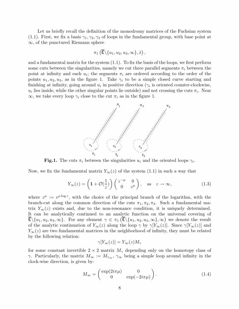
and a fundamental matrix for the system (1.1). To fix the basis of the loops, we first performsome cuts between the singularities, namely we cut three parallel segments πi between thepoint at infinity and each ui; the segments πi are ordered according to the order of thepoints u1, u2, u3, as in the figure 1. Take γi to be a simple closed curve starting andfinishing at infinity, going around ui in positive direction (γi is oriented counter-clockwise,ui lies inside, while the other singular points lie outside) and not crossing the cuts πi. Near∞, we take every loop γi close to the cut πi as in the figure 1.

π

γ

π

γ

π

γ1

1 2

2

3

3

u1 u2 3u

Fig.1. The cuts πi between the singularities ui and the oriented loops γi.

Now, we fix the fundamental matrix Y∞(z) of the system (1.1) in such a way that

Y∞(z) =

(

1 + O(1

z)

)(

z−µ 00 zµ

)

, as z → ∞, (1.3)

where zµ := eµ log z, with the choice of the principal branch of the logarithm, with thebranch-cut along the common direction of the cuts π1, π2, π3. Such a fundamental ma-trix Y∞(z) exists and, due to the non-resonance condition, it is uniquely determined.It can be analytically continued to an analytic function on the universal covering ofCl \{u1, u2, u3,∞}. For any element γ ∈ π1

(

Cl \{u1, u2, u3,∞},∞)

we denote the resultof the analytic continuation of Y∞(z) along the loop γ by γ[Y∞(z)]. Since γ[Y∞(z)] andY∞(z) are two fundamental matrices in the neighborhood of infinity, they must be relatedby the following relation:

γ[Y∞(z)] = Y∞(z)Mγ

for some constant invertible 2 × 2 matrix Mγ depending only on the homotopy class ofγ. Particularly, the matrix M∞ := Mγ∞

, γ∞ being a simple loop around infinity in theclock-wise direction, is given by:

M∞ =

(

exp(2iπµ) 00 exp(−2iπµ)

)

. (1.4)

8

The resulting monodromy representation is an anti-homomorphism:

π1

(

Cl \{u1, u2, u3,∞},∞)

→ SL2(Cl )γ 7→ Mγ

(1.5)

Mγγ = MγMγ. (1.6)

The images Mi := Mγiof the generators γi, i = 1, 2, 3 of the fundamental group, are called

the monodromy matrices of the Fuchsian system (1.1). They generate the monodromy

group of the system, i.e. the image of the representation (1.5). Moreover, due to the factthat, in our particular case, the Ai are nilpotent, satisfy the following relations:

det(Mi) = 1, Tr(Mi) = 2, for i = 1, 2, 3, (1.7)

with Mi = 1 if and only if Ai = 0. Moreover, since the loop (γ1γ2γ3)−1 is homotopic to

γ∞, the following relation holds:

M∞M3M2M1 = 1. (1.8)

A simultaneous conjugation Ai 7→ D−1AiD, i = 1, 2, 3 of the coefficients Ai of the Fuchsiansystem (1.1) by a diagonal matrix D, implies the same conjugation of the monodromymatrices Mγ 7→ D−1MγD, for any γ ∈ π1

(

Cl \{u1, u2, u3,∞},∞)

.We now recall the definition of the connection matrices. Let us assume that Mi 6= 1,

or equivalently Ai 6= 0, for every i = 1, 2, 3. We choose the fundamental matrices Yi(z) ofthe system (1.1), such that:

Yi = Gi (1 + O(z − ui)) (z − ui)J , as z → ui, (1.9)

where J is the Jordan normal form of Ai, namely J =

(

0 10 0

)

, the invertible matrix Gi

is defined by Ai = GiJG−1i , and the choice of the branch of log(z − ui) needed in the

definition of

(z − ui)J =

(

1 log(z − ui)0 1

)

is similar to the one above. The fundamental matrix Yi(z) is uniquely determined up tothe ambiguity:

Yi(z) 7→ Yi(z)Ri,

where Ri is any matrix commuting with J .Continuing, along, say, the right-hand-side of the cut πi, the solution Y∞ to a neigh-

borhood of ui, we obtain another fundamental matrix around ui, that must be related toYi(z) by:

Y∞(z) = Yi(z)Ci, (1.10)

for some invertible matrix Ci. The matrices C1, C2, C3 are called connection matrices, andare related to the monodromy matrices as follows:

Mi = C−1i exp(2πiJ)Ci, i = 1, 2, 3. (1.11)

9

Lemma 1.1. Given three matrices M1, M2, M3, Mi 6= 1 for every i = 1, 2, 3, satisfyingthe relations (1.7) and (1.8), then

i) there exist three matrices C1, C2, C3 satisfying the (1.11). Moreover they are uniquelydetermined by the matrices M1, M2, M3, up to the ambiguity Ci 7→ R−1

i Ci, whereRiJ = JRi, for i = 1, 2, 3.

ii) If the matrices M1, M2, M3 are the monodromy matrices of a Fuchsian system of theform (1.1), then any triple C1, C2, C3 satisfying (1.11) can be realized as the connectionmatrices of the Fuchsian system itself.

Proof. i) By the (1.7), the monodromy matrices have all the eigenvalues equal to one;moreover they can be reduced to the Jordan normal form because Mi 6= 1. Namely thereexists a matrix Ci such that:

Mi = C−1i

(

1 10 1

)

Ci.

Taking

Ci =

(

1 2πi0 1

)

Ci

we obtain the needed matrix. Two such matrices Ci and C′i give the same matrix Mi if and

only if C−1i C′

i commutes with J , namely if and only if they are related by Ci = R−1i C′

i. ii)Let us now assume that C′

1, C′2, C

′3 are the connection matrices of a Fuchsian system of the

form (1.1), with monodromy matrices M1, M2, M3; id est Y∞(z) = Y ′i (z)C′

i, i = 1, 2, 3,for some choice of the solutions Y ′

1 , Y ′2 and Y ′

3 of the form (1.9). We have

Mi = (C′i)

−1 exp(2πiJ)C′i = C−1

i exp(2πiJ)Ci, i = 1, 2, 3.

So the matrices Ri = C′iC

−1i must commute with J and C1, C2, C3 are the connection

matrices with respect to the new solutions Yi(z) = Y ′i (z)Ri. QED

Now, we state the result about the correspondence between monodromy data andcoefficients of the Fuchsian system, for a given set of poles:

Lemma 1.2. Two Fuchsian systems (1.1) with the same poles u1, u2 and u3, and thesame value of µ, coincide if and only if they have the same monodromy matrices M1, M2,M3, with respect to the same basis of the loops γ1, γ2 and γ3.

Proof. Let Y(1)∞ (z) and Y

(2)∞ (z) be the fundamental matrices of the form (1.3) of the two

Fuchsian systems. Let us consider the following matrix:

Y (z) := Y (2)∞ (z)Y (1)

∞ (z)−1.

Y (z) is an analytic function around infinity:

Y (z) = 1 + O(

1

z

)

, as z → ∞.

10

Since the monodromy matrices coincide, Y (z) is a single valued function on Cl \{u1, u2, u3}.Let us prove that Y (z) is analytic also at the points ui. Due to Lemma 1.1, we can choose

the fundamental matrices Y(1)i (z) and Y

(2)i (z) in such a way that

Y (1),(2)∞ (z) = Y

(1),(2)i (z)Ci i = 1, 2, 3.

with the same connection matrices Ci. Then near the point ui,

Y (z) = G(2)i (1 + O(z − ui))

[

G(1)i (1 + O(z − ui))

]−1

.

This proves that Y (z) is an analytic function on all Cl and then, by the Liouville theorem

Y (z) = 1,

and the two Fuchsian systems must coincide.

Corollary 1.1. Two Fuchsian systems (1.1) with the same poles u1, u2 and u3, and thesame value of µ, are conjugated

A(1)i = D−1A(2)

i D, i = 1, 2, 3,

with a diagonal matrix D, if and only if their monodromy matrices M(1)i and M

(2)i , with

respect to the same basis of the loops γ1, γ2 and γ3, are conjugated:

M(1)i = D−1M

(2)i D, i = 1, 2, 3.

1.1.2. The isomonodromy deformations of the Fuchsian system (1.1) and thePainleve equation PVIµ. We now want to deform the poles of the Fuchsian systemkeeping the monodromy fixed. The theory of these deformations is described by the fol-lowing two results:

Theorem 1.1. Let M1, M2, M3 be the monodromy matrices of the Fuchsian system:

d

dzY 0 =

( A01

z − u01

+A0

2

z − u02

+A0

3

z − u03

)

Y 0, (1.12)

of the above form (1.2), with pairwise distinct poles u0i , and with respect to some basis

γ1, γ2, γ3 of the loops in π1

(

Cl \{u01, u

02, u

03,∞},∞

)

. Then there exists a neighborhood

U ⊂ Cl3 of the point u0 = (u0

1, u02, u

03) such that, for any u = (u1, u2, u3) ∈ U , there exists

a unique triple A1(u), A2(u), A3(u) of analytic matrix valued functions such that:

Ai(u0) = A0

i , i = 1, 2, 3,

and the monodromy matrices of the Fuchsian system

d

dzY = A(z; u)Y =

(A1(u)

z − u1+

A2(u)

z − u2+

A3(u)

z − u3

)

Y, (1.13)

11

with respect to the same basis1 γ1, γ2, γ3 of the loops, coincide with the given M1, M2,M3. The matrices Ai(u) are the solutions of the Cauchy problem with the initial data A0

i

for the following Schlesinger equations:

∂

∂uj

Ai =[Ai,Aj]

ui − uj

,∂

∂ui

Ai = −∑

j 6=i

[Ai,Aj]

ui − uj

. (1.14)

The solution Y 0∞(z) of (1.12) of the form (1.3) can be uniquely continued, for z 6= ui

i = 1, 2, 3, to an analytic function

Y∞(z, u), u ∈ U,

such thatY∞(z, u0) = Y 0

∞(z).

This continuation is the local solution of the Cauchy problem with the initial data Y 0∞ for

the following system that is compatible to the system (1.13):

∂

∂ui

Y = −Ai(u)

z − ui

Y.

Moreover the functions Ai(u) and Y∞(z, u) can be continued analytically to global mero-morphic functions on the universal coverings of

Cl3\{diags} :=

{

(u1, u2, u3) ∈ Cl3 | ui 6= uj for i 6= j

}

,

and{

(z, u1, u2, u3) ∈ Cl4 | ui 6= uj for i 6= j and z 6= ui, i = 1, 2, 3

}

,

respectively.

The proof can be found, for example, in [Mal], [Miwa], [Sib]. We recall the theoremof solvability of the inverse problem of the monodromy (see [Dek]):

Theorem 1.2. Given three arbitrary matrices, satisfying (1.7) and (1.8), with M∞ of theform (1.4), and given a point u0 = (u0

1, u02, u

03) ∈ Cl

3\{diags}, for any neighborhood U ofu0, there exist (u1, u2, u3) ∈ U and a Fuchsian system of the form (1.1), with the givenmonodromy matrices, the given µ and with poles in u1, u2, u3.

Remark 1.1. Fuchsian systems of the form (1.1), with coefficients Ai satisfying (1.2),depend on four parameters, one of them being µ. The triples of the monodromy matricessatisfying (1.7) and (1.8), with M∞ of the form (1.4), depend on four parameters too.Loosely speaking, Theorems 1.1 and 1.2 claim that, not only the monodromy matricesare first integrals for the equations of isomonodromy deformation (1.14), but they provide

1 Observe that the basis γ1, γ2, γ3 of π1

(

Cl \{u1, u2, u3,∞},∞)

varies continuously withsmall variations of u1, u2, u3. This new basis is homotopic to the initial one, so we canidentify them.

12

a full system of first integrals for such equations. We denote A(u1, u2, u3;M1,M2,M3)the solution of the Schlesinger equations locally uniquelly determined by the triple ofmonodromy matrices (M1,M2,M3).

All the above arguments remain valid for a general 2 × 2 Fuchsian system, providedthe non-resonancy condition of the eigenvalues of Ai and A∞.

Remark 1.2. We observe that the isomonodromy deformations equations preserve theconnection matrices Ci too. This follows from Lemma 1.1.

1.1.3. Reduction to the PVIµ equation. Let us now explain, following [JMU], howto reduce the Schlesinger equations (1.14) to the PVIµ equation. The Schlesinger equationsare invariant with respect to the gauge transformations of the form:

Ai 7→ D−1AiD, i = 1, 2, 3, for any D diagonal matrix.

First of all we have to factor out such gauge transformations; to this aim, we introducetwo coordinates (p, q) on the quotient of the space of the matrices satisfying (1.2) withrespect to the equivalence relation

Ai ∼ D−1AiD, i = 1, 2, 3, for any D diagonal matrix. (1.15)

The coordinates (p, q) are defined as follows: q is the root of the following linear equation:

[A(q; u1, u2, u3)]12 = 0,

and p is given by:p = [A(q; u1, u2, u3)]11,

where A(z; u1, u2, u3) is given in (1.13). The matrices Ai are expressed rationally in termsof the coordinates (p, q) and an auxiliary coordinate k, coming from the gauge freedom(1.15):

(Ai)11 = − (Ai)22 =q − ui

2µP ′(ui)

P (q)p2 + 2µP (q)

q − ui

p+ µ2(q + 2ui −∑

j

uj)

,

(Ai)12 = −µk q − ui

P ′(ui),

(Ai)21 = k−1 q − ui

4µ3P ′(ui)

P (q)p2 + 2µP (q)

q − ui

p+ µ2(q + 2ui −∑

j

uj)

2

,

(1.16)

for i = 1, 2, 3, where P (z) = (z − u1)(z − u2)(z − u3) and P ′(z) = dPdz

. The Schlesingerequations in these coordinates reduce to:

∂q

∂ui

=P (q)

P ′(ui)

[

2p+1

q − ui

]

∂p

∂ui

= −P ′(q)p2 + (2q + ui −

∑

j uj)p+ µ(1 − µ)

P ′(ui),

(1.17)

13

for i = 1, 2, 3. The system of the reduced Schlesinger equations (1.17) is invariant underthe transformations of the form

ui 7→ aui + b, q 7→ aq + b, p 7→ p

a, ∀a, b ∈ Cl , a 6= 0.

We introduce the following new invariant variables:

x =u2 − u1

u3 − u1,

y =q − u1

u3 − u1;

(1.18)

the system (1.17), expressed in the these new variables, reduces to the PVIµ equation fory(x).

Remark 1.3. The system (1.17) admits the following singular solutions (see [Ok1] and[Wat]):

q ≡ ui for some i,

and p, in the variable x, can be expressed via Gauss hypergeometric functions (see [Ok1]).Moreover the monodromy group of the system (1.1) reduces to the monodromy group ofthe Gauss hypergeometric equation, namely the following lemma holds true:

Lemma 1.3. The solutions of the full Schlesinger equations, corresponding to the solutionq ≡ ui, for some i, have the form:

Ai(u) ≡ 0, and for j 6= i Aj(u) = D(u)−1A0jD(u),

where D(u) is a diagonal matrix depending on u, and A0j is a constant matrix. The

monodromy matrix Mi of the corresponding Fuchsian system turns out to be the identity.Conversely, if one of the monodromy matrices Mi is the identity, Mi = 1, then the solutionof (1.17) is degenerate.

Proof. The matrix Ai, for q ≡ ui, is identically 0, thanks to (1.16). Having Ai ≡ 0, Mi is1. Conversely, if Mi = 1, then Ai ≡ 0. Solving the Schlesinger equations (1.13), we obtainq ≡ ui, and the equation for p is reduced to a Gauss hypergeometric equation. QED

The singular solutions do not give any solution of the PVIµ equation. All the othersolutions do, via (1.18). Conversely, starting from any solution y(x) of PVIµ, we arrive atthe solution:

q = (u3 − u1)y

(

u2 − u1

u3 − u1

)

+ u1

p =P ′(u2)

2P (q)y′(

u2 − u1

u3 − u1

)

− 1

2

1

q − u2

of the reduced Schlesinger equations (1.17). To obtain a solution of the full Schlesingerequations, the function k must be given by a quadrature:

∂k

∂ui

= (2µ− 1)q − ui

P ′(ui).

We conclude this section summarizing all the above results in the following:

14

Theorem 1.3. The branches of solutions of the PVIµ equation near a given point x0 ∈Cl \{0, 1,∞}, are in one-to-one correspondence with the triples of the monodromy matricesM1, M2, M3 satisfying (1.7) and (1.8), with M∞ of the form (1.4), none of them beingequal to 1, considered modulo diagonal conjugations.

Remark 1.4. A triple of 2 × 2 matrices M1,M2,M3 ∈ SL(2; Cl ), considered moduloconjugations, is a point ρ of the space of representations

ρ : F3 → SL(2; Cl )

of the free group F3 with three generators γ1, γ2, γ3, specified by

Mi = ρ(γi), i = 1, 2, 3.

In the general case, i.e. with the matrices Ai and A∞ not necassarly of the form (1.2), thecorresponding solution (p, q) of the reduced Schlesinger equations will be denoted

p = p(u1, u2, u3; ρ), q = q(u1, u2, u3; ρ).

It is locally uniquelly specified by the representation ρ, provided the non-resonancy con-dition of the eigenvalues of Ai and A∞.

1.2. The structure of the analytic continuation.

We parameterized branches of the solutions of PVIµ by triples of monodromy matrices.Now we show how do these parameters change with a change of the branch in the processof analytic continuation of the solutions along a path in Cl \{0, 1,∞}. Recall that, as itfollows from Theorem 1.1, the solutions of PVIµ, defined in a neighborhood of a given pointx0 ∈ Cl \{0, 1,∞}, can be analytically continued to a meromorphic function on the universalcovering of Cl \{0, 1,∞} (the above mentioned Painleve Property). The fundamental groupπ1

(

Cl \{0, 1,∞})

is non-abelian. As a consequence, the global structure of the analyticcontinuation of the solutions of PVI is more involved than that of the other Painleveequations. In fact the solutions of PI,..., PV have at most two critical singularities and thecorresponding fundamental group is abelian.

As a first step we introduce a parameterization of the monodromy matrices.

1.2.1. The parameterization of the monodromy data Let M1, M2 and M3 bethree linear operators Mi : Cl

2 → Cl2 satisfying (1.7). We introduce for them a parameter-

ization which will be useful for studying the analytic continuation of the solutions of thePVIµ equation.

Lemma 1.4. If M1, M2 are such that

Tr(M1M2) 6= 2,

then there exists a basis in Cl2 such that, in this basis, the matrices of M1, M2 have the

form:

M1 =

(

1 −x1

0 1

)

, M2 =

(

1 0x1 1

)

, (1.19)

15

where x1 =√

2 − Tr(M1M2); when M1, M2 are such that Tr(M1M2) = 2, they have

a common eigenvector, and then there exists a basis in Cl2 such that, in this basis, the

matrices M1, M2 are both upper-triangular.

Proof. Due to the (1.7), there exist two vectors e1 and e2 such that

M1e1 = e1, M2e2 = e2.

We now prove that these two vectors are linearly dependent if and only if Tr(M1M2) = 2.In fact if the two vectors are linearly dependent, then we can find a linear independentvector e′2 such that, in the basis (e1, e

′2) the matrices of M1, M2 have the form:

M1 =

(

1 λ1

0 1

)

, M2 =

(

1 λ2

0 1

)

,

so Tr(M1M2) = 2. Conversely, in the basis (e1, e′2) the matrix M1 has the form M1 =

(

1 λ1

0 1

)

and, requiring that

Tr(M1M2) = 2, eigenv(M2) = 1,

also the matrix M2 must have the above form M2 =

(

1 λ2

0 1

)

. Then, the two vectors e1

and e2 are linearly dependent. As a consequence, if Tr(M1M2) 6= 2, the two vectors e1and e2 are linearly independent, and in the basis (e1, e2) the matrices of M1, M2 have theform:

M1 =

(

1 λ1

0 1

)

, M2 =

(

1 0λ2 1

)

,

with Tr(M1M2) = 2 + λ1λ2. Rescaling the basic vectors (e1, e2), we obtain the (1.19).QED

Lemma 1.5. Let M1, M2, M3 satisfy also the condition (1.8) with M∞ given by (1.4),and 2µ 6∈ ZZ. Then the following statements are true:

i) If two of the following numbers

Tr(M1M2), Tr(M1M3), Tr(M3M2)

are equal to 2, then one of the matrices of Mi is equal to one.ii) If Tr(M1M2) 6= 2, then there exists a basis in Cl

2 such that, in this basis, the matricesM1, M2 and M3 have the form

M1 =

(

1 −x1

0 1

)

, M2 =

(

1 0x1 1

)

, M3 =

(

1 + x2x3

x1−x2

2

x1

x23

x11 − x2x3

x1

)

, (1.20)

where

Tr(M1M2) = 2 − x21, Tr(M3M2) = 2 − x2

2, Tr(M1M3) = 2 − x23,

16

andx2

1 + x22 + x2

3 − x1x2x3 = 4 sin2 πµ. (1.21)

iii) If two triples of matrices M1, M2, M3 and M ′1, M

′2, M

′3 satisfying (1.8), with none of

them equal to 1, have the form (1.20) with the parameters (x1, x2, x3) and (x′1, x′2, x

′3)

respectively, then these triples are conjugated

Mi = T−1M ′iT

with some invertible matrix T if and only if the triple (x′1, x′2, x

′3) is equal to the triple

(x1, x2, x3), up to the change of the sign of two of the coordinates.

Proof.i) Let us assume that

Tr(M1M2) = 2, Tr(M1M3) = 2.

Let e1 and e3 be the common eigenvectors of M1, M2 and M1, M3 respectively, (seeLemma 1.4). If M1 6= 1, then the eigenvectors e1 and e3 coincide. Then we can finda linear independent vector e′2 such that, in the basis (e1, e

′2) the matrices of M1, M2,

M3 all have the form

Mi =

(

1 λi

0 1

)

, i = 1, 2, 3.

ThenTr(M3M2M1)1Tr(M∞) = 2.

This contradicts the assumption 2µ 6∈ ZZ.ii) Let us choose the basis such that, according to Lemma 1.4, the matrices M1, M2 have

the form (1.19). Solving the equations

Tr(M3M2) = 2 − x22, Tr(M1M3) = 2 − x2

3,

we arrive at the formula (1.20). The (1.21) is obtained by straightforward computa-tions from

Tr(M3M2M1) = 2 cos 2πµ.

iii) The two triples of matrices M1, M2, M3 and M ′1, M

′2, M

′3 are conjugated

Mi = T−1M ′iT

with some invertible matrix T if and only if they are the matrices of the same operatorsM1, M2, M3, written in different bases. Since the traces do not depend on the choiceof the basis, then

x2i = x′i

2, i = 1, 2, 3.

According to the proof of Lemma 1.4, the basis (e1, e2) is uniquely determined upto changes of sign. A change of sign e1 7→ −e1 corresponds to the change of signx1 7→ −x1; then the form of the matrix M3 is preserved if and only if we change oneof the signs of x2 or x3. QED

17

Remark 1.5. The matrices (1.20) have a simple geometrical meaning. Let us considerthe three-dimensional linear space with a basis (e1, e2, e3) and with a skew-symmetricbilinear form {·, ·} such that

{e1, e2} = x1, {e1, e3} = x3, {e2, e3} = x2.

Let us consider the reflections R1, R2, R3 in this space, with respect to the hyperplanesskew-orthogonal to the basic vectors:

Ri(x) = x− {ei, x}ei, i = 1, 2, 3.

The reflections have a one-dimensional invariant subspace, namely the kernel of the bilinearform. The matrices of the reflections acting on the quotient are the (1.20).

Definition. A triple (x1, x2, x3) is called admissible if it has at most one coordinate equalto zero. Two such triples are called equivalent if they are equal up to the change of twosigns of the coordinates.

Observe that for an admissible triple (x1, x2, x3) none of the matrices (1.20) is equalto the identity. So the admissible triples correspond to the non-singular solutions of thereduced Schlesinger equations (1.17). Moreover, two equivalent triples generate the samesolution. We can summarize the above results in the following:

Theorem 1.4. The branches of solutions of the PVIµ equation near a given point x0 ∈Cl \{0, 1,∞} are in one-to-one correspondence with the equivalence classes of the admissibletriples satisfying (1.21).

Proof. Starting from a solution of PVIµ we obtain the monodromy matrices satisfying(1.7). None of them is equal to the identity. So the canonical form (1.20) of M1,M2,M3 isdetermined uniquely up to a choice of the admissible triple (x1, x2, x3) within the equiva-lence class. Conversely, given an admissible triple (x1, x2, x3) satisfying (1.21), we obtainthe matrices M1,M2,M3 of the form (1.20). The matrix M3M2M1 is diagonalizable withthe eigenvalues exp(±2πiµ) (here we use the non-resonance condition 2µ 6∈ ZZ). Reducingthis matrix to the diagonal form

M3M2M1 = T−1

(

exp(2πiµ) 00 exp(−2πiµ)

)

T

we obtain the monodromy matrices TMiT−1 satisfying (1.7) and thus specifying a branch

of the solution of PVIµ.

1.2.2. Monodromy data and symmetries of PVIµ. The Painleve VI equation pos-sesses a rich family of symmetries, i. e. transformations of the dependent and independentvariables (y, x), and also of the parameters, that preserve the shape of the equation. Thetheory of these symmetries, and its applications to the construction of particular solutions,was developed in [Ok]. Here we list the symmetries which preserve our PVIµ and computetheir action on the monodromy data.

18

First of all we observe that the trivial symmetry µ 7→ 1 − µ preserves the Painleve’equation, i.e. PVIµ = PVI(1 − µ), so it maps the solutions y(x) in themselves.

Then we consider the permutations of the poles u1, u2, u3 which generate the actionof the symmetric group S3 on the solutions y(x). In particular the involution

i1 : u2 ↔ u3,

produces the transformation

x 7→ 1

x, y 7→ y

x, (1.22)

and

i2 : u1 ↔ u3,

produces the transformation

x 7→ 1 − x, y 7→ 1 − y. (1.23)

Both these transformations clearly preserve the equation PVIµ.

Let us compute the action of these symmetries on the monodromy data. The onlything that changes is the basis in the fundamental group π1(Cl \{u1, u2, u3,∞}). In fact,the cuts π1, π2, π3 along which we take our basis γ1, γ2, γ3, are ordered according to theorder of the poles. Applying the transformation i1 we then arrive at the new basis γ′1, γ

′2, γ

′3

shown in figure 2.

u’ u’u == 1u’u u =1

γ,

2 3 3 2

2

1

,γ=γ

13

γ,

=2

γ

γ3

Fig.2. The new basis γ′1, γ′2, γ

′3 obtained by the action of i1.

This new basis has the following form

γ′1 = γ1, γ′2 = γ2γ3γ−12 , γ′3 = γ2.

As a consequence the new monodromy matrices are

M ′1 = M1, M ′

2 = M−12 M3M2, M ′

3 = M2.

19

u’ u’u == u’u u =1 2 3 13 2

2γ,

γ3

,

γ1

γ2

=1

γ,

3γ

Fig.3. The new basis γ′1, γ′2, γ

′3 obtained by the action of i2.

For the second transformation i2, the basis of the new loops is shown in figure 3.

It has the following form

γ′1 = γ3, γ′2 = γ−13 γ2γ3, γ′3 = γ−1

3 γ−12 γ1γ2γ3.

The new monodromy matrices are

M ′1 = M3, M ′

2 = M3M−12 M3, M ′

3 = M3M2M1M−12 M−1

3 .

Lemma 1.6. In the coordinates (x1, x2, x3) on the space of the monodromy matrices, theaction of the symmetries i1, i2 is given by the formulae

i1 : (x1, x2, x3) 7→ (x3 − x1x2,−x2, x1), i2 : (x1, x2, x3) 7→ (−x2,−x1, x1x2 − x3).

The proof is straightforward.

The last symmetry is more complicated because it changes the value of the parameterµ, i.e. µ 7→ −µ, or equivalently µ 7→ 1 + µ as it follows form the fact that PVI(−µ) =PVI(1 + µ). This simmetry comes from the following simultaneous conjugation of thecoefficients of the Fuchsian system:

Ai → ΣAiΣ,

where

Σ = Σ−1 =

(

0 11 0

)

.

Indeed,

ΣA∞Σ = −A∞.

Using the parameterization (1.16) of the matrices A1, A2, A3 by the coordinates (p, q), wearrive at the following

20

Lemma 1.7. The formula

y = y

(

p0(y′)2 + p1y

′ + p2

)2

q0(y′)4 + q1(y′)3 + q2(y′)2 + q3y′ + q4, (1.24)

where

p0 = x2(x− 1)2,

p1 = 2x(x− 1)(y − 1)[2µ(y − x) − y]

p2 = y(y − 1)[y(y − 1) − 4µ(y − 1)(y − x) + 4µ2(y − x)(y − x− 1)]

q0 = x4(x− 1)4

q1 = −4x3(x− 1)3y(y − 1)

q2 = 2x2(x− 1)2y(y − 1)[3y(y − 1) + 4µ2(y − x)(1 + x− 3y)]

q3 = 4x(x− 1)y2(y − 1)2[−y(y − 1) − 16µ3(y − x)2 + 4µ2(y − x)(3y − x− 1)]

q4 = y2(y − 1)2{

y2(y − 1)2 + 64µ3y(y − 1)(y − x)2 − 8µ2y(y − 1)(y − x)(3y − x− 1)+

+ 16µ4(y − x)2[(x− 1)2 + y(2 + 2x− 3y)]}

,

(1.25)transforms solutions of PVIµ to solutions of PVI(−µ). The class of equivalence of themonodromy data (x1, x2, x3) does not change under such a symmetry.

Proof. The new monodromy matrices M ′1,M

′2,M

′3 have the form

M ′i = ΣMiΣ, i = 1, 2, 3.

Then, the canonical form (1.20) of the monodromy operators does not change. QED

Other symmetries are superpositions of (1.24) with the trivial one µ → 1 − µ. Usingthese symmetries, one can transform PVIµ to PVIµ′ , with µ′ = ±µ + n for an arbitraryinteger n.

Remark 1.6. One can show that the above symmetries, and their superpositions, ex-haust all the birational transformations preserving our one-parameter family of PVI equa-tions. We will not do it here (see [Ok]). It is important, however, that these symmetriespreserve the class of algebraic solutions of PVIµ. We will classify all the algebraic solutionsmodulo the above symmetries.

Remark 1.7. It is not difficult to show that the denominator of the formula (1.24) doesnot vanish identically for any solution of PVIµ, with 2µ 6∈ ZZ. Indeed, eliminating yxx andyx form the system

yxx =1

2

(

1

y+

1

y − 1+

1

y − x

)

y2x −

(

1

x+

1

x− 1+

1

y − x

)

yx

+1

2

y(y − 1)(y − x)

x2(x− 1)2

[

(2µ− 1)2 +x(x− 1)

(y − x)2

]

,

21

Q(yx, y, x, µ) =0,

d

dxQ(yx, y, x, µ) =0,

where Q is the denominator, the resultant equation

(2µ+ 1)4µ16[

x(x− 1)2]4

[y(y − 1)(y − x)]4

never vanishes.

1.2.3. The analytic continuation of the solutions of PVIµ and the braid groupB3. In this subsection, we describe the procedure of the analytic continuation towards anaction of the braid group on the admissible triples (x1, x2, x3) parameterizing the branchesof the solutions of PVIµ.

According to Theorem 1.1, any solution of the Schlesinger equations can be continuedanalytically from a point (u0

1, u02, u

03) to another point (u1

1, u12, u

13) along a path

(u1(t), u2(t), u3(t)) ∈ Cl3\{diags}, 0 ≤ t ≤ 1,

withui(0) = u0

i , and ui(1) = u1i ,

provided that the end-points are not the poles of the solution. The result of the analyticcontinuation depends only on the homotopy class of the path in Cl

3\{diags}. Particularly,to find all the branches of a solution near a given point u0 = (u0

1, u02, u

03) one has to

compute the results of the analytic continuation along any homotopy class of closed loopsin Cl

3\{diags} with the beginning and the end at the point u0 = (u01, u

02, u

03). Let

β ∈ π1

(

Cl3\{diags}; u0

)

be an arbitrary loop. Any solution of the Schlesinger equations near the point u0 =(u0

1, u02, u

03), is uniquely determined by the monodromy matricesM1, M2 andM3, computed

in the basis γ1, γ2, γ3. Continuing analytically this solution along the loop β, we arriveat another branch of the same solution near u0. This new branch is specified, accordingto Theorem 1.3, by some new monodromy matrices Mβ

1 , Mβ2 and Mβ

3 , computed in thesame basis γ1, γ2, γ3. Our nearest goal is to compute these new matrices for any loopβ ∈ π1

(

Cl3\{diags}; u0

)

.

The fundamental group π1

(

Cl3\{diags}; u0

)

is isomorphic to the pure (or unper-muted) braid group, P3 with three strings (see [Bir]); this is a subgroup of the full braidgroup B3. The full braid group is isomorphic to the fundamental group of the same spacewhere the permutations are allowed:

B3 ≃ π1

(

Cl3\{diags}

/

S3; u0)

,

S3 being the symmetric group acting by permutations of the coordinates (u1, u2, u3). Anyloop in B3 has the form

(u1(t), u2(t), u3(t)) ∈ Cl3\{diags}, 0 ≤ t ≤ 1,

22

withui(0) = u0

i , ui(1) = u0p(i),

where p is a permutation of {1, 2, 3}. The elements of the subgroup P3 of pure braids arespecified by the condition p = id.

To simplify the computations we extend the procedure of the analytic continuation tothe full braid group

M1, M2, M3 7→Mβ1 , M

β2 , M

β3 , β ∈ B3 = π1

(

Cl3\{diags}

/

S3; u0)

.

For a generic braid β ∈ B3, the new monodromy matrices describe the superposition ofthe analytic continuation and of the permutation

ui 7→ up(i), Ai 7→ Ap(i). (1.26)

The braid group B3 admits a presentation with generators β1 and β2 and the definingrelation

β1β2β1 = β2β1β2.

The generators β1 and β2 are shown in the figure 4.

β

u u u u u u

β

1 2 3 1 2 3

21

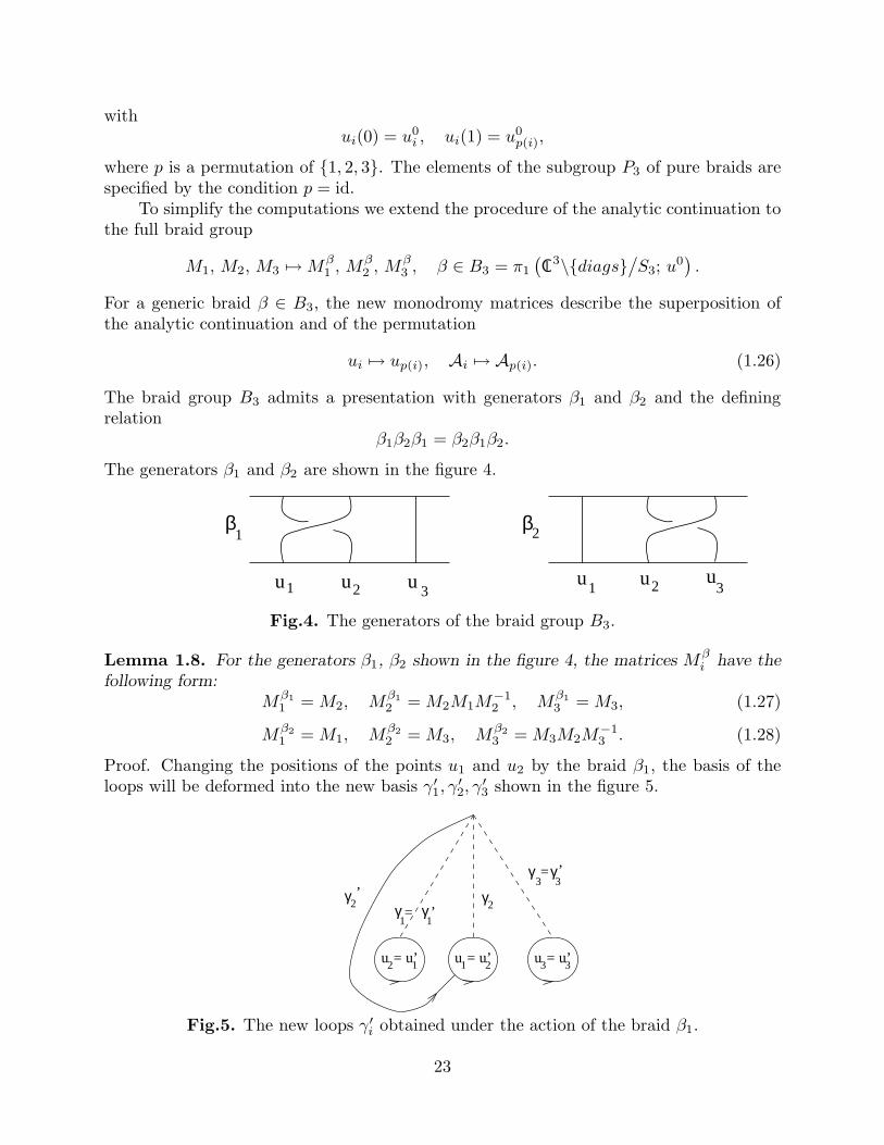
Fig.4. The generators of the braid group B3.

Lemma 1.8. For the generators β1, β2 shown in the figure 4, the matrices Mβi have the

following form:Mβ1

1 = M2, Mβ1

2 = M2M1M−12 , Mβ1

3 = M3, (1.27)

Mβ2

1 = M1, Mβ2

2 = M3, Mβ2

3 = M3M2M−13 . (1.28)

Proof. Changing the positions of the points u1 and u2 by the braid β1, the basis of theloops will be deformed into the new basis γ′1, γ

′2, γ

′3 shown in the figure 5.

u’ u’u =2= 1u’u2 u1= 3 3

γ

γ2

,

γ1

,1

γ

3γ3

,

=

=

2γ

Fig.5. The new loops γ′i obtained under the action of the braid β1.

23

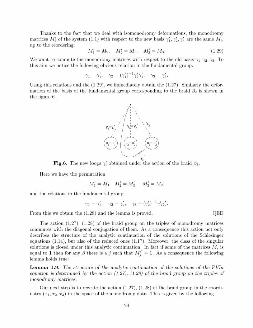
Thanks to the fact that we deal with isomonodromy deformations, the monodromymatrices M ′

i of the system (1.1) with respect to the new basis γ′1, γ′2, γ

′3 are the same Mi,

up to the reordering:M ′

1 = M2, M ′2 = M1, M ′

3 = M3. (1.29)

We want to compute the monodromy matrices with respect to the old basis γ1, γ2, γ3. Tothis aim we notice the following obvious relation in the fundamental group:

γ1 = γ′1, γ2 = (γ′1)−1γ′2γ

′1, γ3 = γ′3.

Using this relations and the (1.29), we immediately obtain the (1.27). Similarly the defor-mation of the basis of the fundamental group corresponding to the braid β2 is shown inthe figure 6.

u’ u’u =2= 1u’u u = 31 3 2

2γ,

γ3

,

γ21γ

,1

γ = = 3γ

Fig.6. The new loops γ′i obtained under the action of the braid β2.

Here we have the permutation

M ′1 = M1 M ′

2 = M ′3, M ′

3 = M2,

and the relations in the fundamental group:

γ1 = γ′1, γ2 = γ′2, γ3 = (γ′2)−1γ′3γ

′2.

From this we obtain the (1.28) and the lemma is proved. QED

The action (1.27), (1.28) of the braid group on the triples of monodromy matricescommutes with the diagonal conjugation of them. As a consequence this action not onlydescribes the structure of the analytic continuation of the solutions of the Schlesingerequations (1.14), but also of the reduced ones (1.17). Moreover, the class of the singularsolutions is closed under this analytic continuation. In fact if some of the matrices Mi isequal to 1 then for any β there is a j such that Mβ

j = 1. As a consequence the followinglemma holds true:

Lemma 1.9. The structure of the analytic continuation of the solutions of the PVIµequation is determined by the action (1.27), (1.28) of the braid group on the triples ofmonodromy matrices.

Our next step is to rewrite the action (1.27), (1.28) of the braid group in the coordi-nates (x1, x2, x3) in the space of the monodromy data. This is given by the following

24

Lemma 1.10. In the coordinates (x1, x2, x3), the action (1.27), (1.28) of the braid groupis given by the formulae:

β1 : (x1, x2, x3) 7→ (−x1, x3 − x1x2, x2),

β2 : (x1, x2, x3) 7→ (x3,−x2, x1 − x2x3).(1.30)

Proof. The above formulae are obtained by straightforward computations from (1.27),(1.28) by means of the parameterization of the monodromy matrices (1.20).

We can summarize the results of this section in the following:

Theorem 1.5. The structure of the analytic continuation of the solutions of the PVIµequation is determined by the action (1.30) of the braid group on the triples (x1, x2, x3).

Remark 1.8. It is easy to see that the braid (β1β2)3 acts trivially on the monodromy

data. This braid is the generator of the center of B3 (see [Bir]). The quotient

B3/center ≃ PSL(2; ZZ)

coincides with the mapping class group of the complex plane with three punctures [Bir].Also in the general case, the structure of analytic continuation of solutions of PVI equationis described by the following natural action ρ → ρβ of the mapping class group on therepresentation space (see remark 1.4)

ρβ(γ) = ρ(β−1⋆ (γ)) (1.31)

whereγ ∈ F3 ≃ π1

(

Cl \{u1, u2, u3,∞},∞)

,

β : Cl \{u1, u2, u3,∞} → Cl \{u1, u2, u3,∞}, β(∞) = ∞is a homeomorphism, and

ρ : F3 → SL(2; Cl ).

Our action (1.30) is obtained restricting (1.31) onto the subspace of representations ofthe form (1.7). The problem of selection of algebraic solutions of Painleve VI (see below)with generic values of the parameters α, β, γ, δ can be reduced to the classification of finiteorbits of the action (1.31).

1.3. Monodromy data and algebraic solutions of the PVIµ equation.

1.3.1. A preliminary discussion on the algebraic solutions of the PVIµ equationand their monodromy data. Here we state some necessary condition for the triples(x1, x2, x3) to generate the algebraic solutions.

Definition. A solution y(x) is called algebraic if there exists a polynomial in two variablessuch that

F (x, y(x)) ≡ 0.

25

If y(x) is an algebraic solution then the correspondent solution p(u), q(u), u =(u1, u2, u3) of the reduced Schlesinger equations (1.17) is also algebraic. According toTheorem 1.1, the solutions of the reduced Schlesinger equations (1.17) can ramify only onthe diagonals u1 = u2, u1 = u3, u3 = u2. Analogously the ramification points of y(x) areallowed to lie only at 0, 1, ∞.

We now characterize the monodromy data such that the correspondent solution of thePVIµ equation is algebraic.

Lemma 1.11. A necessary and sufficient condition for a solution of PVIµ to be algebraicis that the correspondent monodromy matrices, defined modulo diagonal conjugations,have a finite orbit under the action of the braid group (1.27), (1.28).

Proof. By definition, any algebraic function has a finite number of branches. Allowing alsothe permutations (1.26), we still obtain a finite number of values for Mβ

1 , Mβ2 and Mβ

3 ,β ∈ B3 up to diagonal conjugations. QED

Corollary 1.2. An admissible triple (x1, x2, x3) specifies an algebraic solution of PVIµ,with 2µ 6∈ ZZ, if and only if it satisfies (1.21) and its orbit, under the action (1.30) of thebraid group, is finite.

Remark 1.9. We stress that the action (1.30) preserves the relation (1.21).

In this way, the problem of the classification of all the algebraic solutions of the PVIµreduces to the problem of the classification of all the finite orbits of the action (1.30) underthe braid group in the three dimensional space (see [Dub], appendix F). Here we give asimple necessary condition for a triple (x1, x2, x3) to belong to a finite orbit.

Lemma 1.12. Let (x1, x2, x3) be a triple belonging to a finite orbit. Then:

xi = −2 cosπri, ri ∈ Q, 0 ≤ ri ≤ 1, i = 1, 2, 3. (1.32)

Here Q is the set of rational numbers.

Proof. Let us prove the statement for, say, the coordinate x1. Consider the transformation

β21 : (x1, x2, x3) 7→ (x1, x2 + x1x3 − x2

1x2, x3 − x1x2),

as a linear map on the plane (x2, x3). This linear map preserves the quadratic form

x22 + x2

3 − x1x2x3.

If x1 = 2, we put r1 = 1; otherwise we reduce the quadratic form to the principal axes,introducing the new coordinates

x2 =

√2 + x1

2(x2 − x3), x3 =

√2 + x1

2(x2 + x3).

In these new coordinates the preserved quadratic form becomes a sum of squares and thetransformation β2

1 is a rotation by the angle π + 2α, where α is such that x1 = −2 cosα.

26

To have a finite orbit of (x2, x2) under the iterations of β21 , the angle α must be a rational

multiple of π. In this way the statement for x1 is proved. To prove it for x2 and x3 wehave to consider the iterations of β2

2 and β−12 β2

1β2 respectively. QED

Remark 1.10. Thanks to the above lemma, for the finite orbits of the braid group,it is equivalent to deal with the triples (x1, x2, x3), or with the triangles with angles(πr1, πr2, πr3), with xi = −2 cosπri and 0 ≤ ri ≤ 1 (we may assume, changing if necessarytwo of the signs, that at most one of the xi is positive). Observe that the quantity

x21 + x2

2 + x23 − x1x2x3 − 4

is greater than 0 if and only if the triangle (r1, r2, r3) is hyperbolic, namely∑

ri < 1; it isequal to 0, if and only if the triangle (r1, r2, r3) is flat, namely

∑

ri = 1, and it is less than0 if and only if the triangle (r1, r2, r3) is spherical, namely

∑

ri > 1. Thanks to (1.21), aflat triangle gives a resonant value of µ, and it is thus forbidden.

1.3.2. Classification of the triples (x1, x2, x3) corresponding to the algebraicsolutions. We deal with the classification of all the finite orbits of the triples (x1, x2, x3)of the form (1.32), with at most3 one ri being equal to 1

2. According to Lemma 1.12, any

point of these B3-orbits must have the same form (1.32). This condition is crucial in theclassification.

Definition. We say that an admissible triple (x1, x2, x3) is good if for any braid β ∈ B3

one hasβ(x1, x2, x3) = (−2 cosπrβ

1 ,−2 cosπrβ2 ,−2 cosπrβ

3 ),

with some rational numbers 0 ≤ rβi ≤ 1.

Theorem 1.6. Any good triple belongs to the orbit of one of the following five(

−2 cosπ

2,−2 cos

π

3,−2 cos

π

3

)

, (1.33)

(

−2 cosπ

2,−2 cos

π

3,−2 cos

π

4

)

, (1.34)

(

−2 cosπ

2,−2 cos

π

3,−2 cos

π

5

)

, (1.35)

(

−2 cosπ

2,−2 cos

π

3,−2 cos

2π

5

)

, (1.36)

(

−2 cosπ

2,−2 cos

π

5,−2 cos

2π

5

)

. (1.37)

All these orbits are finite and pairwise distinct. They contain all the permutations of thetriples (1.33), (1.34), (1.35), (1.36) and (1.37), and also the triples

(

2 cosπ

3, 2 cos

π

3, 2 cos

π

3

)

, (1.33′)

3 This corresponds to the fact that we deal only with admissible triples.

27

(

−2 cos2π

3,−2 cos

π

4,−2 cos

π

4

)

, (1.34′)

(

−2 cos2π

3,−2 cos

π

5,−2 cos

π

5

) (

−2 cos4π

5,−2 cos

4π

5,−2 cos

4π

5

)

, (1.35′)

(

−2 cos2π

3,−2 cos

2π

5,−2 cos

2π

5

)

,

(

−2 cos2π

5,−2 cos

2π

5,−2 cos

2π

5

)

, (1.36′)

(

−2 cos3π

5,−2 cos

π

3,−2 cos

π

5

)

,

(

−2 cos2π

5,−2 cos

π

3,−2 cos

π

3

)

,

(

−2 cos2π

3, −2 cos

π

3,−2 cos

π

5

)

,

(1.37′)

respectively, together with all their permutations.

Corollary 1.3. There are five finite orbits of the action (1.30) of the braid group on thespace of the admissible triples (x1, x2, x3) satisfying

x21 + x2

2 + x23 − x1x2x3 6= 4.

The lengths of the orbits (1.33), (1.34), (1.35), (1.36) and (1.37), are equal to 4, 9, 10, 10and 18 respectively.

Remark 1.11. The action of the pure braid group P3 on the above orbits gives the sameorbits for any of them but (1.34). The orbit (1.34), under the action of the pure braidgroup P3, splits into three different orbits of three points. So the P3-orbit (1.33) has fourpoints, the three P3-orbits (1.34) have three points each, (1.35) and (1.36) have ten pointseach and (1.37) has eighteen points. These orbits give rise to all the algebraic solutions ofthe PVIµ equation, for µ is given by (1.21). The number of the points of each orbit withrespect to the action of P3 coincides with the number of the branches of the correspondentalgebraic solution.

Proof of Theorem 1.6. The braid group acting on the classes of triples (x1, x2, x3), isgenerated by the braid β1 and by the cyclic permutation:

(x1, x2, x3) 7→ (x3, x1, x2).

As a consequence it suffices to study the operator:

(xi, xj , xk) 7→ (−xi, xj, xk − xixj),

up to cyclic permutations. This transformation works on the triangles with angles πri,πrj, πrk as follows:

(ri, rj, rk) 7→ (1 − ri, rj, r′k), (1.38)

where r′k is such that:cosπr′k = cosπrk + 2 cosπri cosπrj. (1.39)

28

The first step is to classify all the rational triples (ri, rj , rk) such that r′k, defined by (1.39)is a rational number, 1 > r′k > 0, for every choice of i 6= j 6= k 6= i, i, j, k = 1, 2, 3.Equivalently we want to classify all the rational solutions of the following equation:

cosπrk + cosπ(ri + rj) + cosπ(ri − rj) + cosπ(1 − r′k) = 0,

or all the rational quadruples (ϕ1, ϕ2, ϕ3, ϕ4) such that:

cos 2πϕ1 + cos 2πϕ2 + cos 2πϕ3 + cos 2πϕ4 = 0, (1.40)

where the ϕi are related with the ri by the following relations:

ϕ1 = rk/2, ϕ2 =ri + rj

2, ϕ3 =

|ri − rj |2

, ϕ4 =|1 − r′k|

2. (1.41)

Such a classification is given by the following:

Lemma 1.13. The only rational solutions (ϕ1, ϕ2, ϕ3, ϕ4), 0 ≤ ϕi < 1, considered up topermutations and up to transformations ϕi → 1−ϕi, of the equation (1.40) consist of thefollowing non–trivial solutions:

(

1

30,11

30,2

5,1

6

)

(a)

(

7

30,17

30,1

5,1

6

)

(b)

(

1

7,2

7,3

7,1

6

)

(c)

and of the following “trivial” ones, of three types:(d): cos 2πϕ4 = 0. The solutions obtained in [Cro] have the form

(d.1) :

(

1

3,

1

10,

3

10,1

4

)

, (d.2) :

(

ϕ, ϕ+1

3, ϕ+

2

3,1

4

)

, (d.3) :

(

1

4, ϕ, |ϕ− 1

2|, 1

4

)

,

where ϕ is any rational number 0 ≤ ϕ < 1.(e): cos 2πϕ4 = 1. The solutions obtained in [Gor] have the form

(e.1) :

(

1

3,1

4,1

3, 0

)

, (e.2) :

(

1

2, ϕ, |ϕ− 1

2|, 0)

, (e.3) :

(

1

3,1

5,2

5, 0

)

,

where ϕ is any rational number 0 ≤ ϕ < 1.(f): cos 2πϕ1 + cos 2πϕ2 = 0, cos 2πϕ3 + cos 2πϕ4 = 0. The solutions are obvious

ϕ2 = |1/2 − ϕ1|, ϕ4 = |1/2 − ϕ3|,

where ϕ1, ϕ3 are two arbitrary rational numbers 0 ≤ ϕi < 1.

Proof. We follow the idea of Gordan [Gor] (see also [Cro]). In this proof we use the samenotations as in [Cro], except for the ϕi which there are called ri. Let us recall the notations.

29

Let ϕk = nk

dkwhere dk, nk are either positive coprime integers, dk > nk, or nk = 0. Let

p be the largest prime which is a divisor of d1, d2, d3, or d4 and let δk, lk, ck, νk be theintegers such that

dk = δkplk and nk = ckδk + νkp

lk ,

where δk is prime to p, 0 ≤ ck < plk , ck = 0 if lk = 0, but otherwise ck is prime to p. So

ϕk =νk

δk+ckplk

= fk +ckplk

.

We assume that l1 ≥ l2 ≥ l3 ≥ l4 and define the function:

gk(x) =

{

12

[

e2πifkxckpl1−lk + e−2πifkxpl1−ckpl1−lk

]

if ck 6= 0

cos 2πϕk if ck = 0

and, in our case:

U(x) =

4∑

1

gk(x).

As in [Cro], gk

(

exp(

2πipl1

))

= cos 2πϕk and U(

exp(

2πipl1

))

= 0. Let us introduce the

polynomial

P (x) = 1 + xpl1−1

+ x2pl1−1 · · ·x(p−1)pl1−1

.

This is the minimal polynomial of exp(

2πipl1

)

with coefficients in Q, that is such that i)

P(

exp(

2πipl1

))

= 0 and ii) P (x) is irreducible in the ring of polynomials with rational

coefficients. A stronger result was proved by Kronecker (see [Kr]): the polynomial P (x)remains irreducible over any extension of the form Q(ζ1, · · · , ζn), where ζi is a root of theunity of the order coprime with p. As a consequence, the following lemma holds true (see[Gor])

Lemma 1.14. If we express the polynomial U(x) as a sum of polynomials Ut(x),

U(x) =

pl1−1−1∑

t=0

Ut(x),

where Ut(x) contains those terms of U(x) of the form bxc with c = tmod(

pl1−1)

, thenevery Ut(x) is divisible by P (x).

We now apply this lemma in our case. The indices of the powers of x are:

c1, pl1 − c1, c2p

l1−l2 , pl1 − c2pl1−l2 , c3p

l1−l3 , pl1 − c3pl1−l3 , c4p

l1−l4 , pl1 − c4pl1−l4 .

If all the following conditions are satisfied:

l1, l2, l3 > 1, l1 > l2, l3, l4, l2 > l3, l4, l3 > l4, l4 > 0,

30

then there are no indices equal to each other mod(

pl1−1)

and there is no solution of (1.40).So we have to study the cases in which one of them is violated.1): l1 = 1 ≥ l2 ≥ l3 ≥ l4. In this case, since the degree of U(x) is less than p, and thedegree of P (x) is p − 1, being U(x) divisible by P (x), we must have U(x) = mP (x), forsome constant m. There are four possibilities:1.1) : l1 = l2 = l3 = l4 = 1 then U(0) = 0 and P(0)=1. Then m = 0 and U(x) ≡ 0;

moreover if the sum of two (three) terms representing two (three) of the functions gk

vanishes, then the sum of the two (three) functions vanishes. As a consequence thereare only the following possibilities:

1.1.1) : gi = −gj and gk = −gl for some distinct i, j, k, l = 1, · · ·4. This gives rise to thetrivial case (f).

1.1.2) : gl = 0 for some l = 1, · · ·4; this is the trivial case (d).1.1.3) : U(x) contains only two powers of x. If b1, · · · , b4 are the coefficients if one of the

powers xc, then:

b1 + b2 + b3 + b4 = 0, and1

b1+

1

b2+

1

b3+

1

b4= 0,

namely b1, · · · , b4 are the solutions of the following biquadratic equation:

z4 + (b1b2 + b1b3 + b1b4 + b2b3 + b2b4 + b3b4)z2 + b1b2b3b4 = 0.

As a consequence bi + bj = 0, bl + bk = 0, 1bi

+ 1bj

= 0 and 1bl

+ 1bk

= 0, for some

distinct i, j, k, l = 1, · · · , 4. Then this case reduces to the trivial case (f).1.2) l1 = l2 = l3 = 1, l4 = 0; then U(0) = cos 2πϕ4 and then U(x) = cos 2πϕ4P (x), where

P (x) is a polynomial with p powers of x. Since in U we have at most 7 powers and pmust be prime, then p can only be equal to 2, 3, 5, 7.

1.2.1) Case p = 2. Since p is the largest prime in d1, · · · , d4, we must have d1 = d2 = d3 =d4 = 2 and δk = 1. Then νk = 0, ck = 1 and this provides no solution.

1.2.2) Case p = 3. In this case there are the two following possibilities:

1

2e2πif1 +

1

2e2πif2 +

1

2e2πif3 = cos 2πϕ4 =

1

2e−2πif1 +

1

2e−2πif2 +

1

2e−2πif3

or

1

2e−2πif1 +

1

2e2πif2 +

1

2e2πif3 = cos 2πϕ4 =

1

2e2πif1 +

1

2e−2πif2 +

1

2e−2πif3 .

In both the case one can show that there are no solutions. In fact, for example, in thefirst case one has to solve the following equations:

2 cos 2πϕ4 = cos 2πf1 + cos 2πf2 + cos 2πf3, sin 2πf1 + sin 2πf2 + sin 2πf3 = 0.

Using the classification of all the possible rational solution (d.1), (d.2), (d.3) of thecase (d), one can show that there are no solutions.

31

1.2.3) Case p = 5. In this case we have:

1

2e2πifk =

1

2e−2πifk =

1

2e2πifi +

1

2e±2πifj = cos 2πϕ4,

for some distinct i, j, k = 1, 2, 3. Then fk is 0 or 12

and ϕ4 = 16

or ϕ4 = 13

respectively.Following the same computations of [Cro] we obtain the two solutions (a) and (b).

1.2.4) Case p = 7. In this case we have:

1

2e2πif1 =

1

2e−2πif1 =

1

2e2πif2 =

1

2e−2πif2 =

1

2e2πif3 =

1

2e−2πif3 = cos 2πϕ4,

which has the following solutions:

f1 = f2 = f3 = 0 and ϕ4 =1

6or f1 = f2 = f3 =

1

2and ϕ4 =

1

3.

This gives the solution (c).1.3) l1 = l2 = 1 and l3 = l4 = 0. Then U(x) = (cos 2πϕ3 + cos 2πϕ4)P (x); again in U we

have at most 5 powers and then p = 2, 3, 5. The case p = 2 is treated as in [Cro];1.3.1) : In the case p = 3 either

1

2e2πif1 +

1

2e2πif2 =

1

2e−2πif1 +

1

2e−2πif2 = cos 2πϕ3 + cos 2πϕ4,

or:1

2e2πif1 +

1

2e−2πif2 =

1

2e−2πif1 +

1

2e2πif2 = cos 2πϕ3 + cos 2πϕ4.

In the former case, for f1 = f2, with cos 2πf2 = cos 2πϕ3 + cos 2πϕ4 and this givesagain the solution (b). The latter case is equivalent.

1.3.2) : In the case p = 5 one has:

1

2e2πif1 =

1

2e−2πif1 =

1

2e2πif2 =

1

2e−2πif2 = cos 2πϕ3 + cos 2πϕ4,

which gives f1 = f2 = 0 or f1 = f2 = 12 . We treat the former case (the latter is

equivalent); then cos 2πϕ3 + cos 2πϕ4 = 12

and we can show that this case reduces tothe trivial solutions (d) and (e).

1.4) l1 = 1 and l2 = l3 = l4 = 0. In this case, as in [Cro], there is no solution, but thetrivial one (d).

2) l1 ≥ 2, l1 ≥ l2, l3, l4. This case can be treated as the analogous one in [Cro]. Thisconcludes the proof of Lemma 1.13. QED

We now use the above lemma to classify all the triangles which correspond to goodtriples. Every quadruple generates twelve triangles. In fact, given a solution (ϕ1, · · · , ϕ4)we have six ways to choose the pair (ϕi, ϕj) such that

cos 2πϕi + cos 2πϕj = 2 cosπ(ϕi + ϕj) cosπ(ϕi − ϕj).

32

Chosen the pair (ϕi, ϕj), we have two ways for choosing ϕk, in order to have the triangle

(2ϕk, ϕi + ϕj , |ϕi − ϕj |) . (1.42)

The remaining ϕl is, by definition, such that the above triangle is mapped, by the braid(1.38), to:

(|ϕi − ϕj |, |1− ϕi − ϕj |, |1 − 2ϕl|) .

Let us analyze all the triangles generated by the solutions of the equation (1.40), and keepthe good ones, namely the ones for which the new r′k, given by (1.39), is rational for everyi, j, k, cyclic permutation of 1, 2, 3.

In order to do this, observe that if there exists a permutation p such that the triple(rp(1), rp(2), rp(3)) gives via (1.41) values of ϕ1, ϕ2, ϕ3 such that there is not any rational ϕ4

such that ϕ1, ϕ2, ϕ3, ϕ4 satisfy (1.40), then (r1, r2, r3) is not a good triple. In fact, everypermutation p is generated by ciclic permutations and the permutation p23 : (r1, r2, r3) →(r1, r3, r2). Cyclic permutations are elements of the braid group, so the statement isobvious for them. For p23, the statement is a trivial consequence of the fact that thetriples (r1, r2, r3) and (r1, r3, r2) give via (1.41) the same values of ϕ1, ϕ2, ϕ3.

So we will exclude all the triangles (r1, r2, r3) for which there exists at least a permu-tation that gives rise to values of (ϕ1, ϕ2, ϕ3) for which rational solutions ϕ4 of (1.40) donot exist.

Solution (a). Using (1.42), we obtain the triangles

(

1

15,

1

30,23

30

)

,

(

1

15,1

5,

8

15

)

,

(

1

15,

7

30,17

30

)

,

(

4

15,

7

30,13

30

)

,

(

11

15,11

30,13

30

)

,

(

11

15,

2

15,1

5

)

,

(

4

5,

2

15,1

5

)

,

(

1

5,1

5,

7

15

)

,

(

1

3,11

30,13

30

)

,

(

2

3,

1

30,

7

30

)

,

(

1

3,1

5,3

5

)

,

(

1

3,1

3,2

5

)

.

The last two points(

1

3,1

5,3

5

) (

1

3,1

3,2

5

)

(1.43)

belong to the orbit (1.37). The above values suitably permuted, except the (1.43), giverise via (1.41), to the following values of (ϕ1, ϕ2, ϕ3) (written in the same order as thecorrespondent generating triangles)

(

1

60,

5

12,

7

20

)

,

(

1

10,

3

10,

7

30

)

,

(

7

60,19

60,1

4

)

,

(

7

60,

7

20,

1

12

)

,

(

11

60,

7

12,

3

20

)

,

(

1

10,13

30,

3

10

)

,

(

1

15,1

2,

3

10

)

,

(

0,1

5,

7

30

)

,

(

1

20,11

60,23

60

)

,

(

1

60,

9

20,13

60

)

.

33

there isn’t any rational number ϕ4 such that any of the quadruples build with these triplesand ϕ4 is in the class described by Lemma 1.13.

Solution (b). Using (1.42), the triangles are

(

7

15,11

30,23

30

)

,

(

7

15,2

5,11

15

)

,

(

7

15,

1

30,11

30

)

,

(

2

15,

1

30,19

30

)

,

(

2

15,

1

30,17

30

)

,

(

2

15,

1

15,3

5

)

,

(

2

5,

1

15,2

5

)

,

(

2

5,11

15,2

5

)

,

(

1

3,

1

30,13

30

)

,

(

1

3,11

30,23

30

)

,

(

2

5,1

3,4

5

)

,

(

1

3,1

3,4

5

)

.

The last two points are equivalent to:

(

1

3,1

5,3

5

) (

2

3,1

3,1

5

)

(1.44)

of the orbit (1.37). As before one can show that if (r1, r2, r3) is one of the above values,except the (1.44), then there exists a permutation such that the r′k defined by (1.39) isno-more rational. In fact we obtain for example the following values of (ϕ1, ϕ2, ϕ3), whichdon’t fall in the values obtained in Lemma 1.13:

(

11

60,37

60,

3

20

)

,

(

1

5,3

5,

2

15

)

,

(

1

60,

5

12,

1

20

)

,

(

1

60,3

4,23

60

)

,

(

1

60,47

60,

7

20

)

,

(

1

30,23

30,11

30

)

,

(

1

30,2

5, 0

)

,

(

11

30,2

5, 0

)

,

(

1

60,23

60,

1

20

)

,

(

11

60,11

20,13

60

)

.

Solution (c).

(

2

7,1

7,5

7

)

,

(

2

7,

5

42,19

42

)

,

(

2

7,11

42,25

42

)

,

(

4

7,11

42,25

42

)

,

(

4

7,2

7,4

7

)

,

(

4

7,

1

42,13

42

)

,

(

1

7,

1

42,29

42

)

,

(

1

7,

5

42,23

42

)

,

(

1

7,1

7,4

7

)

,

(

1

3,1

7,3

7

)

,

(

1

3,2

7,4

7

)

,

(

1

3,1

7,5

7

)

.

As before one can show that if (r1, r2, r3) is one of the above values then there exists apermutation such that the r′k defined by (1.39) is no more rational. In fact we obtain forexample the following values of (ϕ1, ϕ2, ϕ3), which are not included in the values describedby Lemma 1.13:

(

1

14,1

2,

3

14

)

,

(

5

84,31

84,

1

12

)

,

(

11

84,37

84,13

84

)

,

(

11

84,

7

12,

1

84

)

,

(

1

7,4

7, 0

)

,

(

1

84,37

84,11

84

)

,

(

1

84,

5

12,23

84

)

,

(

5

84,29

84,17

84

)

,

34

(

1

7,2

7, 0

)

,

(

1

14,

8

21,

1

21

)

,

(

1

7,19

42,

5

42

)

,

(

1

14,11

21,

4

21

)

.

Solution (d.1).

(

2

3,

3

20,

3

20

)

,

(

1

3,

1

20,

9

20

)

,

(

1

5,

1

20,

1

20

)

,

(

1

5,

1

30,19

30

)

,

(

1

5,

1

12,

7

12

)

,

(

2

5,

1

12,

5

12

)

,

(

3

5,

3

20,

7

20

)

,

(

3

5,

7

30,13

30

)

,

(

1

2,

7

30,13

30

)

,

(

1

2,

1

30,11

30

)

,

(

2

3,1

5,2

5

)

,

(

1

2,1

5,2

5

)

.

The last two points are equivalent to:

(

1

3,1

5,3

5

) (

1

2,2

5,1

5

)

(1.45)

of the orbit (1.37), which is now complete. We can again exclude all the other values of(r1, r2, r3), with the same trick as above.

Solution (d.2). In this case we have that any of the triangles generated is equivalent toone of the following:

(

|1 − 2ϕ|, |1 − 4ϕ|4

,1 + 4ϕ

4

)

,

(

1

2,|1 − 4ϕ|

4,|3 − 4ϕ|

4

)

,

(

1

2,|1 − 4ϕ|

4,1 + 4ϕ

4

)

,

(

2ϕ,|1 − 4ϕ|

4,|3 − 4ϕ|

4

)

,

(

1

2,1

2,|1 − 4ϕ|

2

)

,

where ϕ is an arbitrary rational number. The last triangle is forbidden because it has tworight angles, and the first four ones are all equivalent to a flat triangle, so they are againforbidden because they give rise to a an half-integer value of µ.

Solution (d.3). The generated triangles are the following:

(

1

2,1

3, 2ϕ+

1

3

)

,

(

|23− 2ϕ|, 1

3, 2ϕ+

1

3

)

,

(

1

2,2

3,2

3+ 2ϕ

)

,

(

2

3+ 2ϕ,

2

3,2

3+ 2ϕ

)

,

(

2

3+ 2ϕ,

|1 − 4ϕ|4

,1 + 4ϕ

4

)

,

(

|23− 2ϕ|, |1 − 4ϕ|

4,1 + 4ϕ

4

)

,

(

1

2,1

3, 1 + 2ϕ

)

,

(

2ϕ,1

3, 1 + 2ϕ

)

,

(

|23− 2ϕ|, ϕ+

1

12, ϕ+

7

12

)

,

(

2ϕ, ϕ+1

12, ϕ+

7

12

)

,

(

2

3+ 2ϕ, ϕ+

5

12, ϕ+

11

12

)

,

(

2ϕ, ϕ+5

12, ϕ+

11

12

)

.

35

This case must be studied carefully because we have to classify the allowed values of therational variable ϕ in order that, applying the transformation (1.38), we obtain alwaysrational values.

Let us analyze the first triangle. It is mapped by (1.38) to a triangle equivalent to thesecond:

(

1

2,1

3, 2ϕ+

1

3

)

7→(

1

3+ 2ϕ,

2

3, 2ϕ+

1

3

)

∼(

|23− 2ϕ|, 1

3, 2ϕ+

1

3

)

. (1.46)

If we apply the braid (1.38), with ri = 2π3 , rj = rk = 2ϕ+ 1

3 , we have to solve:

cos2π

3+ 2 cos2 π(2ϕ+

1

3) = cosπr′k,

or, equivalently, for ϕ and for the new ϕk:

cos2π

3+ cos 2π(2ϕ+

1

3) + 1 + cos 2πϕk = 0.

We classify the values of the allowed ϕ using the Lemma 1.13 in the case (e). We have sixpossibilities for ϕ:

i) if ϕk = 12, then ϕ = 11

24. In this case we obtain, from (1.46), all the points of the orbit

(1.34).ii) if ϕk = 1

4 , then ϕ = 0. In this case we obtain, from (1.46), all the points of the orbit(1.33).

iii) if ϕk = 12 , then ϕ = 1

4 . In this case we obtain, from (1.46), the following points:

(

1

2,1

3,5

6

)

,

(

1

6,2

3,1

6

)

.

We exclude them because there exists a permutation such that the r′k defined by (1.39)is no-more rational.

iv) if ϕk is free to vary, then 2ϕ+ 13 = 1

2 . In this case we obtain, from (1.46), the forbiddenpoint:

(

1

2,1

3,1

2

)

,

so we have to exclude it.v) if ϕk = 1

5 , then ϕ = 130 , and we obtain, from (1.46), the following two points of the

orbit (1.36):(

1

2,1

3,2

5

)

,

(

2

5,2

3,2

5

)

.

vi) if ϕk = 25 , then ϕ = 13

30 , and we obtain the following two points of the orbit (1.35):

(

1

2,1

3,1

5

)

,

(

1

5,2

3,1

5

)

.

36

In the same way we can study all the other triangles and show that we don’t obtainany other value but the ones described in Theorem 1.6.

Solution (e.1). The generated triangles are the following:

(

0, 0,2

3

)

,

(

0,1

12,

7

12

)

,

(

0,1

2,2

3

)

,

(

2

3,

1

12,

7

12

) (

2

3,1

3,1

3

)

,

(

1

2,1

3,1

3

)

,

(

2

3,1

4,1

4

)

;

the first four are forbidden because there exists a permutation such that the r′k defined by(1.39) is no-more rational. So we have to exclude them. The fifth and the sixth are pointsof the orbit (1.33) and the last of (1.34).

Solution (e.2). The generated triangles are the following:

(

2ϕ,1

2,1

2

)

,

(

|1 − 2ϕ|, 12,1

2

)

,

(

1

2,1

2,|1 + 4ϕ|

2

)

, (1, ϕ, ϕ) ,

(

1,|1 − 2ϕ|

2,|1 − 2ϕ|

2

)

,

(

0,1

2,|1 − 4ϕ|

2

)

, (|1 − 2ϕ|, ϕ, ϕ) ,

(

0,|1 − 2ϕ|

2,1 + 2ϕ

2

)

,

(0, ϕ, 1− ϕ) ,

(

2ϕ,|1 − 2ϕ|

2,|1 − 2ϕ|

2

)

,

(

|1 − 2ϕ|, |1 − 2ϕ|2

,1 + 2ϕ

2

)

, (2ϕ, ϕ, 1 − ϕ) ,

They are all forbidden, the first three because they have two right angles, the next threeones, because we can prove that necessarily ϕ = 1

2 , then the first has two right angles, thesecond gives | cosπr′k| = 3 and the last gives | cosπr′k| = 2; all the others because they areequivalent to a flat triangle.

Solution (e.3). The generated triangles are the following:

(

0,2

15,

8

15

)

,

(

0,1

15,11

15

)

,

(

0,1

5,3

5

)

,

(

2

3,1

5,3

5

)

,

(

2

5,

1

15,11

15

)

,

(

4

5,

2

15,

8

15

)

,

(

4

5,1

5,1

5

)

,

(

2

3,1

5,1

5

)

,

(

2

3,2

5,2

5

)

,

(

2

5,2

5,2

5

)

,

(

2

5,1

3,1

3

)

,

(

1

5,2

3,1

3

)

.

We exclude the first six because we can show that there exists a permutation such thatthe r′k defined by (1.39) is no-more rational. The seventh and the eighth give two pointsof the orbit (1.36), the ninth and tenth two points of the orbit (1.39) and the last two, twopoints of (1.39).

Solution (f) We have obtained all the points of all the orbits of Theorem 1.6. To showthat there are no other points we still have to examine the case (f). In this case all theobtained triangles are equivalent to the following:

(

ϕ1

2,|2 − ϕ1 + ϕ3|

4,|2 − ϕ1 − ϕ3|

4

)

,

(

ϕ1

2,1

2,|1 − ϕ1|

2

)

,

(

ϕ1

2,|4 − ϕ1 − ϕ3|

4,|ϕ1 − ϕ3|

4

)

.

(1.47)

37

Applying the transformation (1.38) to the above triangles, we find that we have to solvefor ϕ1, ϕ3 and for the new ϕ obtained from the (1.39), the following three equationsrespectively:

cosπ|2 − ϕ3|

2+ cosπϕ1 + cos 2πϕ+ 1 = 0,

cosπ|1 + ϕ1 − ϕ3|

2+ cosπ

|1 − ϕ1 − ϕ3|2

+ cos 2πϕ = 0,

2 cosπϕ1 + ϕ3

4+ cosπ

|3ϕ1 − ϕ3|4

+ cos 2πϕ = 0.

We again can use Lemma 1.13 to prove that we don’t obtain any new point. Let us showthis in for the first triangle

(

ϕ1

2,|2 − ϕ1 + ϕ3|

4,|2 − ϕ1 − ϕ3|

4

)

. (1.48)

We have to solve the equation

cosπ|2 − ϕ3|

2+ cosπϕ1 + cos 2πϕ+ 1 = 0. (1.49)

Using Lemma 1.13, the possible values for ( |2−ϕ3|2

, ϕ1, ϕ) are the (e.1), (e,2) and (e.3).Consider the case (e.1), then the possible solutions for the pair (ϕ1, ϕ3), are

(ϕ1, ϕ3) = (1

2,2

3), (

2

3, 1), (

2

3,2

3).

Let us substitute these solutions in (1.48); we obtain the triangles

(1

4,13

24,

5

24), (

1

3,

7

12,

1

12), (

1

3,1

2,1

6),

which are all flat, and thus forbidden. Let us now consider the case (e.2). In this case weobtain two possibilities: either ϕ3 = 0 and ϕ1 is a free parameter, or ϕ1 = 1 and ϕ1 is afree parameter. In both the cases the triangle (1.48) is flat, and thus forbidden. Let usnow consider the last case (e.3). The possible solutions for the pair (ϕ1, ϕ3), are

(ϕ1, ϕ3) = (2

5,2

3), (

2

3,6

5), (

2

5,2

5), (

4

5,6

5), (

4

5,2

3), (

2

3,2

5).

Substituting these values in (1.48), we obtain all flat angles. We can repeat the same prooffor the other two triangles in (1.47). In this way we conclude the proof of the theorem.QED

1.4. Monodromy data and reflection groups.

We reformulate here the above parameterization of the monodromy data by classes ofequivalence of triples (x1, x2, x3) in a geometric way. Let us consider a three-dimensional

38

space V with a basis (e1, e2, e3) and with a symmetric bilinear form (·, ·) given, in thisbasis, by the matrix

g :=

2 x1 x3

x1 2 x2

x3 x2 2

(1.50)

namely

(ei, ei) = 2, for i = 1, 2, 3, and (e1, e2) = x1, (e2, e3) = x2, (e1, e3) = x3.

Observe that the bilinear form (1.50) does not degenerate. Indeed,

det g = 8 − 2(x21 + x2

2 + x23 − x1x2x3) = 8 cos2 πµ 6= 0,

due to the non-resonance assumption 2µ 6∈ ZZ. The three planes p1, p2, p3 orthogonal tothe basic vectors (e1, e2, e3) possess the following properties:1) The normal vectors to these planes are non-isotropic (i.e. (ei, ei) 6= 0).2) None of the planes is orthogonal to the other two.

Conversely, a three-dimensional space V with a non-degenerate symmetric bilinearform (·, ·) and with an ordered triple of planes satisfying the above conditions, uniquelydetermines the matrix g of the form (1.50), and then the monodromy data of a solution ofPVIµ.

We define three reflections R1, R2, R3 with respect to the three planes (p1, p2, p3):

Ri :V → V

x 7→ x− (ei, x)ei

i = 1, 2, 3.

These reflection have the following matrix representation in the basis (e1, e2, e3):

R1 =

−1 −x1 −x3

0 1 00 0 1

, R2 =

1 0 0−x1 −1 −x2

0 0 1

, R3 =

1 0 00 1 0

−x3 −x2 −1

.

(1.51)Let us consider the group G ⊂ O(V, (·, ·)) of the linear transformations of V , generatedby the three reflections R1, R2, R3. The matrix g will be called the Gram matrix of thereflection group G. It determines the subgroup G ⊂ O(V, (·, ·)) uniquely. We observethat, for an admissible triple, the group G is irreducible, namely there are no non-trivialsubspaces of V which are invariant with respect to all the transformations of G.

We conclude that the branches of the solutions of PVIµ can be parameterized bygroups G ⊂ O(3) with a marked ordered system of generating reflections R1, R2, R3. Letus describe what happens with the triples of generators under the analytic continuation ofthe solution.

We define an action of the braid group B3 on the systems of generators R1, R2, R3 ofthe reflection group G:

β1 : (R1, R2, R3) 7→ (R1, R2, R3)β1 :=(R2, R2R1R2, R3),

β2 : (R1, R2, R3) 7→ (R1, R2, R3)β2 :=(R1, R3, R3R2R3),

(1.52)

where β1,2 are the standard generators of the braid group. Observe that the groups gen-erated by the reflections (R1, R2, R3) and (R1, R2, R3)

β coincide for any β ∈ B3. Inparticular the following lemma holds true:

39

Lemma 1.15. For any braid β ∈ B3, the transformations β(R1, R2, R3) are reflections

with respect to some planes orthogonal to some new basic vectors (eβ1 , e

β2 , e

β3 ). The Gram

matrix with respect to the basis (eβ1 , e

β2 , e

β3 ) has the form:

(eβi , e

βi ) = 2, i = 1, 2, 3, (eβ

1 , eβ2 ) = xβ

1 , (eβ2 , e

β3 ) = xβ

2 , (eβ1 , e

β3 ) = xβ

3 ,

where (xβ1 , x

β2 , x

β3 ) = β(x1, x2, x3).

Proof. It is sufficient to check the statement for the generators β1,2. For β = β1:

eβ1

1 = e2, eβ1

2 = e1 − x1e2, eβ1

3 = e3,

for β = β2:eβ2

1 = e1, eβ2

2 = e3, eβ2

3 = e2 − x2e3.

Computing the Gram matrix we prove the lemma. QED

1.4.1. Reflection groups and algebraic solutions Let us figure out what are thereflection groups corresponding to the finite orbits classified in Theorem 1.6.

Theorem 1.7. The orbit (1.33) corresponds to the group W (A3) of symmetries of regulartetrahedron, the orbit (1.34) corresponds to the group W (B3) of symmetries of the regularoctahedron, the orbits (1.35), (1.36), (1.37) correspond to different choices of a system ofgenerating reflections in the group W (H3) of symmetries of icosahedron.

Proof. It is sufficient to find one point in each of the orbits (1.33), (1.34), (1.35), (1.36),(1.37) that corresponds to a triple of symmetry planes of a regular polyhedron. To thisend, we associate to a regular polyhedron a standard triple of symmetry planes usingthe following construction. Let 0 be the center of the polyhedron. Take a face of thepolyhedron and denote H the center of this face, P a vertex and Q the center of an edge ofthe face passing through the vertex P . The standard triple consists of the symmetry planestrough the points OPQ, OQH, OHP respectively. Let us compute the angles betweenthe planes of each regular polyhedron. It is convinient to use the Schlafli symbol {p, q} forregular polyhedra (see [Cox]). In these notations, the face of the regular polyhedron {p, q}is a regular p-gon, the vertex figure is a regular q-gon. We immediately see that the anglesbetween the planes of the standard triple are

between OPQ and OQHπ

2,

between OQH and OHPπ

p,

between OHP and OPQπ

q.

So, for the tetrahedron {3, 3} we obtain the angles(

π2 ,

π3 ,

π3

)

, for the octahedron {3, 4} the

angles(

π2, π

3, π

4

)

, for the icosahedron {3, 5} the angles(

π2, π

3, π

5

)

. In this way, we obtain thetriples (1.33), (1.34), (1.35). The reciprocal polyherda (i.e. cube {4, 3} and dodecaherdon

40

{5, 3}) give the same angles up to permutations. As we already know, the permutedtriples of (1.34) or (1.35) belong to the same orbit. So, the standard triples of cube anddodecahedron are B3-equivalent to those of octahedron and icosahedron respectively.

To obtain the last two orbits (1.36) and (1.37), we apply the above construction ofthe standard triple to great icosahedron and dodecahedron respectively. These non convexregular polyhedra both have icosaherdal symmetry (see [Cox]). Their Schlafli symbols are{

3, 52

}

and{

5, 52

}

respectively. This means that the faces of these polyhedra are regulartriangles or pentagons, but the vertex figures are pentagrams. The above computationgives the triples (1.36) and (1.37). Again we need not consider the reciprocal stellatedpolyhedra. Theorem 1.7 is proved. QED

1.4.2. Classification of the monodromy data, second proof. We present hereanother proof of Theorem 1.6, based on the idea suggested by E. B. Vinberg. We startwith the following:

Algebraic Lemma. Let (x, y, z) be an admissible triple of real numbers, satisfying theinequalities:

x2 + y2 + z2 − xyz > 4, (1.53)

and

|x|, |y|, |z| ≤ 2. (1.54)

Then there exists a braid β ∈ B3 such that the absolute value of some of the coordinatesof β(x, y, z) is strictly greater than 2.

Before proving the lemma, we observe that we can assume, without loss of generality,that all the coordinates of (x, y, z) are non-zero; in fact, for any admissible triple, thereexists a braid β ∈ B3 such that all the coordinates of β(x, y, z) are non-zero. Let us denotebx, by and bz the following braids:

bx := β2, bx(x, y, z) = (z,−x, x− yz),by := β−1

2 β1β2, by(x, y, z) = (−y + xz,−x,−z),bz := β1, bz(x, y, z) = (−x, z − xy, y).

Lemma 1.16. Let (x, y, z) be a triple of non-zero real numbers, satisfying

0 < |z|, |x|, |y| ≤ 2 (1.55)

and

x2 + y2 + z2 − xyz = 4 + c2, c > 0. (1.56)

Denote (x′, y′, z′) := β(x, y, z), where

β =

bx if |x| ≤ |y|, |z|,by if |y| ≤ |x|, |z|,bz if |z| ≤ |x|, |y|.

41

Then:min{|x′|, |y′|, |z′|} ≥ min{|x|, |y|, |z|} (1.57)

and|x′| + |y′| + |z′| ≥ |x| + |y|+ |z| + min{z2, 2c}. (1.58)

Proof. Let us prove the lemma in the case where |z| ≤ |x|, |y| and β = bz. The other casescan be proved in the same way. If the signs of z and of xy are opposite then

|y′| = |z| + |xy| ≥ |z| + z2, |x′| = |x|, |z′| = |z|

and (1.57), (1.58) are proved. Let us suppose that the signs of z and of xy are the same.Changing the triple (x, y, z) to an equivalent one, we can assume that all the coordinatesare positive. If we prove now that

2z + 2c ≤ xy, (1.59)

where c is given in (1.56), we have that |y′| = |xy − z| ≥ z + 2c and the lemma is proved.To prove (1.59) we find the constrained minimum of the function xy on the domain Ddefined by the conditions (1.55) and (1.56). The Lagrange function

F (x, y, z) := xy − λ(

x2 + y2 + z2 − xyz)

,

has the local maximum at

x = y =

√

4 + c2 − z2

2 − z,

and no minimum in the interior of D. It remains to study the values of the function xy onthe boundary of D. If, say, z = y then the positive root x of the equation

x2 + 2z2 − xz2 = 4 + c2

is greater than 2. So the boundaries z = y and z = x are not reached for (x, y, z) ∈ D,and then |z| < |x|, |y|. It remains the last boundary to be studied. If, say, y = 2, we findx = z ± c. Since x ≥ z, then x = z + c and xy = 2(z + c); this is the minimum of thefunction xy. QED

Proof of Algebraic Lemma. As observed above we can always reduce to the case where allthe coordinates (x, y, z) are non-zero. Put:

∆(x, y, z) := min{

x2, y2, z2, 2√

x2 + y2 + z2 − xyz − 4}

.

Using Lemma 1.16, we can build a braid b1 such that the coordinates:

(x1, y1, z1) := b1(x, y, z)

satisfy the inequalities

min{|x1|, |y1|, |z1|} ≥ min{|x|, |y|, |z|} |x1|+|y1|+|z1| ≥ |x|+|y|+|z|+∆(x, y, z). (1.60)

42

Since the quantity x2 + y2 + z2 − xyz− 4 is preserved by the action of the braid group, weobtain:

∆(x1, y1, z1) ≥ ∆(x, y, z).

If the absolute value of some of the coordinates (x1, y1, z1) is greater than 2, the lemma inproved. Otherwise we apply again the construction of Lemma 1.16 to the triple (x1, y1, z1).In this way we obtain a sequence of braids b1, b2, b3 · · · such that the corresponding triples

(xk+1, yk+1, zk+1) := bk+1(xk, yk, zk)

satisfy∆(xk+1, yk+1, zk+1) ≥ ∆(xk, yk, zk).

Iterating the inequality (1.57), we obtain that

|xk| + |yk| + |zk| ≥ |x| + |y| + |z| + k∆(x, y, z).

Hence, in a finite number of steps we build a triple such that the absolute value of at leastone of the coordinates in greater than 2. This concludes the proof of Algebraic Lemma.QED

Corollary 1.4. For an algebraic solution of PVIµ, specified by an admissible triple xi =−2 cos 2πri, the value of µ must be real, the strict inequalities

|xi| < 2, i = 1, 2, 3, (1.61)

hold true and the matrix g defined in (1.50) is positive definite.

Proof. Let us prove that, for an algebraic solution, the triple (x1, x2, x3) must satisfy theinequality:

x21 + x2

2 + x23 − x1x2x3 < 4. (1.62)

Indeed, if x21 + x2

2 + x23 − x1x2x3 > 4, then, according to the Algebraic Lemma the triple

is not a good one. This contradicts the assumption that the solution is algebraic. Ifx2

1 + x22 + x2

3 − x1x2x3 = 4, then µ = 12 + k with k ∈ ZZ. This contradicts the basic

assumption 2µ 6∈ ZZ. Then (1.62) is satisfied and µ is a real number. Let us now prove(1.61). If one of the coordinates, say x1, is such that x1 = ±2, then

x21 + x2

2 + x23 − x1x2x3 = 4 + (x2 ∓ x3)

2,

and, being x2 x3 real numbers, (1.62) is violated. So, xi 6= ±2 for every i. Finally, applyingthe Sylvester criterion to the matrix g, we prove that g is positive definite. In fact

detG = 8 − 2(x21 + x2

2 + x23 − x1x2x3) > 0,

and for any principal minor

det

(

2 xi

xi 2

)

= 4 − x2i > 0.

QED

43

Lemma 1.17. For an algebraic solution of PVIµ the reflection group G acts in the Eu-clidean space.

The proof immediately follows from the fact that the correspondent Gram matrix is positivedefinite.

Corollary 1.5. For a good triple (x1, x2, x3) and for any braid β ∈ B3, there exists three

integer positive numbers nβ12, n

β13 and nβ

23 such that:

(

Rβi R

βj

)nβ

ij

= 1, for i 6= j, i, j = 1, 2, 3. (1.63)

Proof. If (e1, e2) = x1 = −2 cosπr with r = mn

, m,n ∈ ZZ, then R1R2 is a rotation by theangle 2πm

n. Hence:

(R1R2)n

= 1.

This holds true for any pair Ri and Rj . Moreover, for any braid β ∈ B3, the tripleβ(x1, x2, x3) is again good, then (1.63) is proved. QED

Corollary 1.6. The set of the solutions of the PVIµ equation with a real non resonantvalue of µ and real parameters (x1, x2, x3) satisfying

|xi| < 2, i = 1, 2, 3,

is invariant with respect to the analytic continuation.

Proof. Applying the Sylvester criterion to the matrix g defined in (1.50), we obtainthat g is positive definite. So the reflections R1, R2, R3 can be realized in the Euclideanspace. After a transformation (x1, x2, x3) 7→ (xβ

1 , xβ2 , x

β3 ) = β(x1, x2, x3), the new numbers

(x1β , x2

β , x3β) are the entries of the Gram matrix:

gβ :=

2 xβ1 xβ

3

xβ1 2 xβ

2

xβ3 xβ

2 2

,

of the basis (eβ1 , e

β2 , e

β3 ), in the same Euclidean space. Then this matrix must be positive

definite, namely x2i < 4 as we wanted to prove. QED

In the second part of this paper, we will identify the set described in Corollary 1.6with the class of solutions of PVIµ having asymptotic behaviour of algebraic type. Thisidentification will be crucial in the computation of the five algebraic solutions of PVIµ wehave classified.

As we have just shown, a good triple

(x1, x2, x3) =

(

−2 cosπm1

n1,−2 cosπ

m2

n2,−2 cosπ

m3

n3

)

,

44

corresponds to a representation of the Coxeter group generated by three reflections R1,R2, R3 satisfying

R21 = R2

2 = R23 = 1, (R1R2)

n1 = (R2R3)n2 = (R1R3)

n3 = 1, (1.64)

in the three-dimensional Euclidean space. We denoted by G the image of this representa-tion. Moreover, for any braid β ∈ B3, the matrices

(Rβ1 , R

β2 , R

β3 ) := β(R1, R2, R3),

satisfy the same identities (1.64), with some new integers nβ1 , n

β2 , n

β3 . We stress that the

reflections Rβ1 , R

β2 , R

β3 generate the same group G.

Theorem 1.8. It follows from the above property that G is an irreducible finite Coxetergroup.

Let n be the least common multiple of n1, n2 and n3. Put:

ζ = 2 cosπ

n.

Lemma 1.18. The numbers

xi = −2 cosπmi

ni

, i = 1, 2, 3,

belong to the ring K0 of integers of the field K := Q[ζ].

Recall (see [Wey]) that K is the normal extension of Q generated by ζ and K0 is thering of all the algebraic integer numbers of K, namely it consists of all the elements x ∈ Ksatisfying an algebraic equation of the form

xk + a1xk−1 + · · · + ak = 0, with ai ∈ ZZ.

Proof of Lemma 1.18. Let n = nim′i, then

cosπmi

ni

= Tmim′

i

(

cosπ

n

)

= Tmim′

i

(

1

2ζ

)

,

where

Tk(x) = cos(k arccosx) = 2k−1xk +

k−1∑

s=0

2s−1aksxs, (1.65)

are the Tchebyscheff polynomials of the first kind (see [Bat]). Recall that all the coefficientsaks are integers, so xi = −2 cosπmi

niis a polynomial of ζ with integer coefficients. Moreover

ζ is a root of the monic algebraic equation with integer coefficients

2Tn

(

ζ

2

)

+ 2 = ζn +

n−1∑

s=0

ansζs + 2 = 0.

45

Hence ζ ∈ K0 and xi = −2Tmim′

i

(

ζ2

)

∈ K0, as we wanted to prove. QED

Proof of Theorem 1.8. From the formulae (1.51) it follows that the matrices R1, R2 andR3 are all defined over the same ring K0 of integers of K:

Ri ∈ Mat(K0, 3).

Moreover, these matrices are orthogonal with respect to g:

RTi gRi = g, (1.66)

where g is defined in (1.50). LetΓ := Gal(K,Q)

the Galois group of K over Q, namely the group of all automorphisms

φ : K → K,

identical on Q.For any φ ∈ Γ we denote φ(Ri) and φ(g) the matrices obtained from Ri and g by the

action(x1, x2, x3) 7→ (φ(x1), φ(x2), φ(x3)). (1.67)

Lemma 1.19. For any φ ∈ Γ the following statements hold true:i) detφ(g) 6= 0,ii) The matrices φ(Ri) are orthogonal with respect to φ(g).iii) For any β ∈ B3 the matrices φ(Ri)

β satisfy the Coxeter relation (1.63).

The proof is obvious, due to the fact that any automorphism preserves all the algebraicrelations.

From the above lemma, and from Algebraic Lemma, it follows that for any φ ∈ Γ,the real symmetric matrix φ(g) must be positive definite. We will show that this impliesthat the group G is finite. Let N be the order of the Galois group Γ. We construct theblock-diagonal matrices

Ri ∈ Mat(K0, 3N), i = 1, 2, 3,

as the matrices formed by 3× 3 blocks on the diagonal, such that the j-th block is φj(Ri),for φj ∈ Γ, j = 1, 2, · · · , N . The matrices Ri are orthogonal with respect to G, that is theblock-diagonal matrix having φj(G), for φj ∈ Γ, j = 1, 2, · · · , N , on the diagonal blocks.We can apply Lemma 1.19 to the matrices Ri to show that they satisfy the Coxeter relation(1.63). As a consequence we obtain a representation of our reflection group G into theorthogonal group

G→ O(

K3N ,G)

Ri 7→ Ri.(1.68)

By construction the matrices Ri preserve the sublattice

K3N0 ⊂ K3N

46

of the vectors the components of which are algebraic integers of the field K. We recall(see [Wey]) that the ring K0 of the algebraic integers of the field K, is a finite-dimensionallattice. As a consequence, the image of the representation (1.68) is a discrete subgroup ofthe orthogonal group. Since G is positive definite, the orthogonal group is compact and,hence, G must be finite. The theorem is proved. QED

To complete the classification of the monodromy data related to the algebraic solutionsit remains to classify the objects

(G,R1, R2, R3),

where G is one of the Coxeter groups A3, B3 and H3 and (R1, R2, R3) is a triple ofgenerating reflections considered modulo the action (1.52) of the braid group. This canbe done by a straightforward computation of all the orbits of the triples of generatingreflections. All of them were described and classified by Schwartz (see the introduction).We arrive again at the list of Theorem 1.6, where, as we already know, the triples (1.33)generate the group W (A3) of the symmetries of the tetrahedron, (1.34) generate the groupW (B3) of the symmetries of the cube, while (1.35), (1.36) and (1.37) correspond to threeinequivalent triples of the generating reflections of the group W (H3).

2. GLOBAL STRUCTURE OF THE SOLUTIONS OF PAINLEVE’ VIµ HAV-ING CRITICAL BEHAVIOUR OF ALGEBRAIC TYPE

In the first part of this paper, we found a class of solutions of PVIµ invariant with respectto the analytic continuation. For them, the reflection group G acts in the three-dimensionalEuclidean space. Recall that the parameter µ must be real, the coordinates of the admis-sible triples (x1, x2, x3) must be real and satisfy the inequality

−2 < xi < 2, i = 1, 2, 3.

In this second part, we prove that this class of solutions coincides with the class of thesolutions of PVIµ having critical behaviour of the algebraic type

y(x) =

a0xl0 (1 + O(xε)) , as x→ 0,

1 − a1(1 − x)l1 (1 + O((1 − x)ε)) , as x→ 1,

a∞x1−l∞

(

1 + O(x−ε))

, as x→ ∞,

(2.1)

where ε > 0 is small enough, the indices l0, l1, l∞ are real and the coefficients a0, a1, a∞are some complex numbers. We compute the behaviour of any branch of these solutionsnear the critical points. These results will be used to compute explicitly all the algebraicsolutions classified in the first part.

47

First of all, we fix the notations. Let us choose:

u1 = 0, u2 = x, u3 = 1.

Then the Fuchsian system (1.1) reads

d

dzY = A(z, x)Y =

(A1

z+

A2

z − x+

A3

z − 1

)

Y,

and, puttingA1 := A0, A2 := Ax, A3 := A1, A∞ = A∞,

we obtaind

dzY =

(

A0

z+

A1

z − 1+

Ax

z − x

)

Y. (2.2)

The branch cuts in Cl are the same as in Section 1.1. We call now the basic loops γ0, γx, γ1.They are fixed as before, namely γ0, γx, γ1 play the role of the preceding γ1, γ2, γ3 (seefigure 1). The Schlesinger equations read:

d

dxA0(x) = − [A0, Ax]

x,

d

dxA1(x) = − [A1, Ax]

x− 1,

d

dxAx(x) =

[A0, Ax]

x+

[A1, Ax]

x− 1.

(2.3)

The correspondent monodromy matrices are

M0, Mx, M1,

which play the role of the preceding M1,M2,M3 respectively. We recall that they satisfy

M∞M1MxM0 = 1, det(Mi) = 1, Tr(Mi) = 2, for i = 0, 1, x, (2.4)

with

M∞ =

(

exp(2iπµ) 00 exp(−2iπµ)

)

. (2.5)

With the above choice of A∞, A1, Ax and A0, satisfying

detAi = 0, Tr(Ai) = 0, i = 0, 1,∞, (2.6)

the non-singular solution A(z, x) of the Schlesinger equations turns out to be related tothe solution of PVIµ in the following way (see [JMU]):

[A(y, x)]12 = 0, iff y(x) solves PVIµ, (2.7)

where y is not identically equal to 0, 1, x.We now state the first main theorem of this second part:

48

Theorem 2.1. For any admissible triple (x0, x1, x∞), xi ∈ lR, |xi| < 2 for i = 0, 1,∞,there exists a unique branch y(x; x0, x1, x∞) of a solution of PVIµ, with the parameter µsatisfying the equation:

4 sin2 πµ = x20 + x2

1 + x2∞ − x0x1x∞, (2.8)

with the asymptotic behaviour (2.1) near the critical points 0, 1,∞. The indices are givenby

li =1

πarccos(cos 2πri) =

2ri if 0 < ri ≤1

2

2 − 2ri if1

2≤ ri < 1

i = 0, 1,∞, (2.9)

withxi = −2 cosπri, i = 0, 1,∞,

and the leading coefficients a0, a1, a∞ are single-valued functions of the equivalence classof x0, x1, x∞ and of µ. Namely, the coefficient a0, for x0 6= 0 , is given by:

a0 =exp(−iπφ)

4(2µ+ l0 − 1)2Γ2(1 − l0)Γ

2( 1+l02

)Γ( 1+l02

+ µ)Γ( 1+l02

− µ)

Γ2(l0)Γ2( 1−l02 )Γ( 1−l0

2 + µ)Γ( 1−l02 − µ)

(2.10)

where

exp(iπφ) =x2

0x21 − 2x2

1 − 2x0x1x∞ + 2x2∞ + ix1sign(x0)

√

4 − x20(2x∞ − x0x1)

2(x21 − x0x1x∞ + x2

∞)(2.11)

and for x0 = 0

a0 =x2∞

x21 + x2

∞. (2.12)

The coefficient a1 is given by the same formula with the substitution x0 ↔ x1, l0 7→ l1; a∞ isgiven by the same formula too, after the substitution (x0, x1, x∞) 7→ (x∞,−x1, x0−x1x∞)and l0 7→ l∞. Conversely any solution of the PVIµ equation, with a real value of µ, havingcritical behaviour of algebraic type, can be obtained by the above construction.

Remark 2.1. The relation (2.8) determines µ up to the transformations

µ 7→ ±µ+ n, n ∈ ZZ.

According to the results of Section 1.2, such an ambiguity can be absorbed by the actionof a symmetry on PVIµ. Recall that these symmetries preserve the class of the algebraicsolutions.

Theorem 2.1 will be proved in Section 2.4.

2.1. Local theory of the solutions of PVIµ having critical behaviour of algebraictype

2.1.1. Local asymptotic behaviour around 0. In this section we characterize thelocal asymptotic behaviour of the solutions of PVIµ near the singular point x = 0. First ofall let us characterize the type of asymptotic behaviour that can be related to the algebraicsolutions.

49

Lemma 2.1. Let y(x) be an algebraic solution of PVIµ. Then the first term of its Puiseuxseries is

y(x) ∼ a0x1−σ0 as x→ 0. (2.13)

for some constant a0 6= 0 and the rational number σ0 must satisfy 0 ≤ σ0 < 1, with a0 6= 1if σ0 = 0.

Proof. If y(x) is an algebraic function, then it admits an expansion in Puiseux seriesaround 0

y(x) =

∞∑

k=k0

akxkn , k0 ∈ ZZ, ak0

6= 0,

where n is some natural number. As a consequence, for k0 6= 0, we have the followingrelation between the orders of the first and second derivative of y:

O(x2y′′) = O(xy′) = O(y) = O(

xk0n

)

. (2.14)

We now reduce to the common denominator the PVIµ equation and collect together allthe terms of the same order in the numerator N , using the rule (2.14). The numerator is

N =2y′2x4 − y′

2x3 − y′

2x5 + 2y′

2x2y − 2y′x3y − 2y′

2x3y + 2y′′x3y + 2y′x4y − 2y′

2x4y−

− 4y′′x4y + 2y′2x5y + 2y′′x5y + xy2 − 2y′xy2 − 2x2y2 + 4µx2y2 − 4µ2x2y2+

+ 6y′x2y2 − 3y′2x2y2 − 2y′′x2y2 − 2y′x3y2 + 6y′

2x3y2 + 2y′′x3y2 − 2y′x4y2−

− 3y′2x4y2 + 2y′′x4y2 − 2y′′x5y2 − 8µxy3 + 8µ2xy3 + 2y′xy3 + 4x2y3−

− 8µx2y3 + 8µ2x2y3 − 6y′x2y3 + 2y′′x2y3 + 4y′x3y3 − 4y′′x3y3 + 2y′′x4y3−− y4 + 4µy4 − 4µ2y4 − 3xy4 + 16µxy4 − 16µ2xy4 − 2x2y4 + 4µx2y4−− 4µ2x2y4 + 2y5 − 8µy5 + 8µ2y5 + 2xy5 − 8µxy5 + 8µ2xy5 − y6 + 4µy6 − 4µ2y6.

The first term of the Puiseux series must be chosen in order to kill the lowest term in thenumerator of the PVIµ equation. If k0 < 0, the lowest term is

−y6 + 4µy6 − 4µ2y6

which, for 2µ 6∈ ZZ cannot be zero for any choice of a0 6= 0. Then k0 cannot be negative. Ifn ≥ k0 > 0, the lowest order term is

2x2y′2y − 2xy′y2 − 2x2y′′y2,

which is zero for any y = ak0x

k0n . For k0 > n, the lowest order term is

−x3y′2

+ 2x3y′′y + xy2,

which cannot be zero. Furthermore, for k0 = 0, the lowest order term in the numerator Nis

−a40(a0 − 1)2(2µ− 1)2

50

and, due to the assumptions 2µ 6∈ ZZ and a0 6= 0, the only possible value of a0 is 1.

Substituting y = 1 + a1xk1n , we obtain that the lowest order term in the numerator N is

x2k1

n a21(k1/n+ 1 − 2µ)(k1/n− 1 + 2µ)

that is zero, for generic values of µ, only if a1 is 0. If µ = 12 ± k1

2n, we can again repeat the

procedure. The numerator will be

N = − 4µ2y2 − 16µ2y3 − 24µ2y4 − 16µ2y5 − 4µ2y6 + y2x+ 8µ2y2x+ 2y3x+ 24µ2y3x+

+ y4x+ 24µ2y4x+ 8µ2y5x+ 2yy′x+ 4y2y′x+ 2y3y′x− y2x2 − 4µ2y2x2 − 2y3x2−− 8µ2y3x2 − y4x2 − 4µ2y4x2 − 6yy′x2 − 12y2y′x2 − 6y3y′x2 − y′

2x2 − 4yy′

2x2−

− 3y2y′2x2 + 2yy′′x2 + 4y2y′′x2 + 2y3y′′x2 + 6yy′x3 + 10y2y′x3 + 4y3y′x3+

+ 3y′2x3 + 10yy′

2x3 + 6y2y′

2x3 − 6yy′′x3 − 10y2y′′x3 − 4y3y′′x3 − 2yy′x4−

− 2y2y′x4 − 3y′2x4 − 3y2y′

2x4 + 6yy′′x4 + 8y2y′′x4 + 2y3y′′x4 + y′

2x5+

+ 2yy′2x5 − 2yy′′x5 − 2y2y′′x5

where µ = ± k1

2nand y = y − 1. Substituting y = a1x

k1n , the lowest order term in the

numerator N is automatically zero. Now, we want to eliminate the next lowest orderterm. Observe thet, now

O(x2y′′) = O(xy′) = O(y) = O(

xk1n

)

.

For the sake of definitess, suppose 12 < µ ≤ 1, i.e. µ = k1

2n< 1

2 (the case µ = − k1

2nis

analogous). The next lowest order terms in the numerator N are

−16µ2y3 + 4xy2y′ − 4x2yy′2+ 4x2y2y′′ + xy2 + 8xµ2y2 − 6x2yy′ + 3x3y′

2 − 6x3yy′′

To eliminate them, we substitute y = 1 + a1xk1n + a1y

k2n , for some k2 > k1. The above

terms give

−4a31(k1

n)2x3

k1n + O(x1+2

k1n )

that is zero if and only of a1 = 0. So we obtain the forbidden solution y(x) ≡ 1. So, k0

can not be zero, and y(x) satisfies (2.13) with 0 < l = k0

n≤ 1, namely 0 ≤ σ0 < 1. QED

In the above lemma we have seen the expected asymptotic behaviour of the algebraicsolutions. We now state the main result of this section, which is more general, namely itholds also for non algebraic solutions.

Theorem 2.2. For any pair of values (a0, σ0), 0 ≤ σ0 < 1, there exists a unique branchof the solution of PVIµ, for a fixed µ, with the asymptotic behaviour

y(x) = a0x1−σ0(1 + xεf(x)) as x→ 0, (2.15)

51

for some ε > 0 and f(x) smooth function such that limx→0 f(x) = const.

In order that x1−σ0 is well defined, we have to make some cut in the complex plane.From now on, we cut along the line argx = ϕ for some ϕ.

Remark 2.2. Theorem 2.2 can be proved also for complex values of the index σ0, pro-vided that 0 ≤ Reσ0 < 1. For algebraic solutions the index σ0 must be a rational number.Because of this, we consider only real indices.

2.1.2. Proof of the existence. First of all we state the existence of solutions of theSchlesinger equations with a particular asymptotic behaviour. The following result willplay an important role also in Section 2.3.

Lemma 2.2 (Sato-Miwa-Jimbo). Given three constant matrices A0i , i = 0, 1, x with

zero eigenvalues such that Λ = A00+A0

x has eigenvalues ±σ2 , 0 ≤ σ < 1, and A0

1 = −Λ−A∞,

in any sector of Cl containing none of the branch cuts, and sufficiently close to 0, thereexists a solution of the Schlesinger equations that satisfy

|A1(x) − A01| ≤ K|x|1−σ′ ∣

∣x−Λ(A1(x) − A01)x

Λ∣

∣ ≤ K|x|1−σ′

(2.16)

∣

∣x−ΛA0(x)xΛ −A0

0

∣

∣ ≤ K|x|1−σ′ ∣

∣x−ΛAx(x)xΛ − A0x

∣

∣ ≤ K|x|1−σ′

, (2.17)

where K is some positive constant and 1 > σ′ > σ.

We want to show that it is possible to choose A0,1,x and Λ such that the correspondingsolution y(x) of the Painleve VI equation obtained via (2.7) has the asymptotic behaviour(2.15). Let us consider an arbitrary constant matrix Λ with eigenvalues ±σ

2 ; let T be thediagonalizing matrix of Λ, namely

Λ = T

(

σ2

00 −σ

2

)

T−1.

Now, we choose A01 = −A∞ − Λ and A0

0,x such that A00 +A0

x = Λ, namely

A00 =

1

2Λ + F, A0

x =1

2Λ − F

for some constant matrix F . Then:

T−1A00T =

(

σ4 00 −σ

4

)

+E, T−1A0xT =

(

σ4 00 −σ

4

)

− E,

where we can choose E =

(

0 bσ4−σ

4b0

)

, for some non-zero constant b. With this choice of

E, A0 and Ax have zero eigenvalues. Using Lemma 2.2, we obtain that, as x→ 0:

A0,x → T

(

xσ2 0

0 x−σ2

)[(

σ4 00 −σ

4

)

±(

0 bσxσ

4−σx−σ

4b0

)](

x−σ2 0

0 xσ2

)

T−1,

52

andA1 → −A∞ − Λ.

Substituting such asymptotic behaviors in the relation (2.7), taking T12, T11 6= 0 we obtain:

y(x) ∼ −T12x1−σ

4bT11; (2.18)

we are now free to choose the arbitrary constants b, T11, T12, σ in such a way that − T12

4bT11=

a0, σ = σ0, for any fixed a0 and σ0.Remark 2.3. Other existence results for σ ∈ Cl \{] − ∞, 0] ∪ [1,+∞[} can be found in[IKSY] and [S1], [S2], [S3]. For indices with Reσ 6∈ [0, 1], the asymptotics obtained inthese papers are valid in more complicated domains near 0.

2.1.3. Proof of the uniqueness. Now we prove that the solution y(x), x ∈ B(0, r), ofPainleve VI equation such that it satisfies (2.15) for some given constants a0 and σ0 ∈ [0, 1),is uniquely determined by a0 and σ0. Here B(0, r) =

{

x∣

∣|x| ≤ r, argx 6= ϕ, x 6= 0}

.The proof is based on the fact that Painleve VI is equivalent to the following reducedSchlesinger equations (1.17):

q =(q − 1)q + 2p(q − 1)q(q − x)

(x− 1)x,

p =−p2(x− 2q − 2xq + 3q2) − p(2q − 1) − (1 − µ)µ

(x− 1)x,

where:

q = y, p =x(x− 1)y − y(y − 1)

2(y − x)y(y − 1), (2.19)

and the dot means the derivative ddx

We shall prove the local uniqueness of the solutionsof the Hamiltonian system with the following asymptotic behaviour

q(x) ∼ axl + xl+ε f(x) p(x) ∼ l − 1

2a

1

xl+xεg(x)

xl(2.20)

where l = 1 − σ0, a = a0, ε > 0 and f(x) and g(x) are some smooth functions in B(0, r)which tend to zero as x→ 0.

This is equivalent to show the theorem. In fact, from the uniqueness of q it followstrivially the uniqueness of y. The following lemma holds true:

Lemma 2.3. The estimates (2.20) on the asymptotic behaviour of (q(x), p(x)) are a con-sequence of (2.15).

Proof. Since q = y, the assertion on y is obvious due to the hypothesis (2.15). Concerningp, we use its definition

p =x(x− 1)y − y(y − 1)

2(y − x)y(y − 1)

53

and by a straightforward computation we show (2.20) for p. QED

We now distinguish two cases: 0 < l < 1, and l = 1. Let us consider the former case;it is convenient to introduce the new variables (q, p)

q =y

xlp = xlp;

which have a similar asymptotic behaviour

q(x) = a+ xεf(x) p(x) =l − 1

2a+ xεg(x), (2.21)

and the equations of the motion become

˙q = fq(p, q, x, xl),

˙p = fp(p, q, x, xl),

(2.22)

with

fq =−q(l − 1 − 2pq)

x− q(1 + 2pq)

x1−l+q(1 + 4pq) − 2x−lpq − xlq2(1 + 2pq)

1 − x,

and

fp =p(l − 1 − 2pq)

x+µ− µ2 + 2pq + 3p2q2

x1−l+

p2

xl − p(1 + 4pq) + xl(µ− µ2 + 2pq + 3p2q2)

1 − x.

We want to prove the uniqueness of the solution (q, p) of (2.22), satisfying (2.21) forx ∈ B(0, r), in the ball ||p− l−1

2a||, ||q−a|| ≤ Cr, for a constant Cr vanishing when the radius

r → 0. Here ||f || = supB(0,r) |f(x)|. Let us suppose that there are two solutions (q1, p1)

and (q2, p2) of the system (2.22), satisfying (2.21). Then, if we define X =

(

q1 − q2p1 − p2

)

, we

obtain, as a consequence of (2.21), that the following limits exist

lim|x|→0, arg(x)=ϑ

X(i)(x)

|x|ε = 0, i = 1, 2, (2.23)

for some 0 < ε, X(i) being the i-th component of X. Moreover, X satisfies the following

X′ =

(

[1−l+2p1(q1+q2)](q1−q2)+2q22(p1−p2)

x+ ∆Q1

x1−l + ∆Q2

xl + ∆Q3

[l−1−2q2(p1+p2)](p1−p2)−2p21(q1−q2)

x+ ∆P1

x1−l + ∆P2

xl + ∆P3

)

,

where

∆Qi = Qi(q1, p1, x) −Qi(q2, p2, x), and ∆Pi = Pi(q1, p1, x) − Pi(q2, p2, x),

54

Q1 = q(1+2pq), Q2 = −2pq, Q3 = q(1+4pq)−2x1−lpq−xlq2(1+2pq)1−x

, P1 = µ−µ2 +2pq+3p2q2,

P2 = p2, P3 = p2x1−l−p(1+4pq)+xl(µ−µ2+2pq+3p2q2)1−x

.We want to prove that, under the hypothesis (2.23), X ≡ 0 (this is equivalent to prove

our theorem). Performing the constant linear transformation X = T Z, where

T =

(

1 01−l2a2

12a2

)

,

we obtain

Z′ =

(

[1−l+2p1(q1+q2)](q1−q2)+2q22(p1−p2)

x+ ∆Q1

x1−l + ∆Q2

xl + ∆Q3

2a2G(p1,p2,q1,q2)x

+ 2a2∆P1+(l−1)∆Q1

x1−l + 2a2∆P2+(l−1)∆Q2

xl + 2a2∆P3 + (l − 1)∆Q3

)

(2.24)where

G(p1, p2, q1, q2) =[l − 1 − 2q2(p1 + p2)](p1 − p2) − 2p21(q1 − q2)}+

+ (l − 1){[1 − l + 2p1(q1 + q2)](q1 − q2) + 2q22(p1 − p2),

and, from (2.23):

lim|x|→0, arg(x)=ϑ

Z(i)(x)

|x|ε = 0, i = 1, 2. (2.25)

In order to prove that Z ≡ 0, we fix any direction in the complex plane arg(x) = ϑ forsome fixed ϑ, and we consider the real variable t = |x|. Then we define:

V(i)(t) := |Z(i)(x)|.We want to prove that the assumption V(i)(t0) 6= 0 for some t0 > 0 leads to a cotradiction.To this aim we prove a differential inequality for the right derivative D+V(i) of V (i)(t).Since D+V(i) ≤ |Z(i)′ |, to obtain such a differential inequality it is enough to estimatefrom above the modulus of the components of the right-hand-side of (2.24). To this aimwe notice that all the polynomials Qi, Pi have the form:

Qi =

3∑

k,n=0

aik,np

nqk, Pi =

3∑

k,n=0

bik,npnqk,

with ak,n(x), bk,n(x) regular functions x ∈ B(0, r). As a consequence, we obtain, in theball ||p− l−1

2a||, ||q − a|| ≤ Cr, the estimates:

|∆Qi|, |∆Pi| ≤ ci1|Z(1)| + ci2|Z(2)| (2.26)

for some positive constants ci1, ci2. In fact

|∆Qi| =∣

∣

∑

k,n

ak,n[qk1 (pn

1 − pn2 ) + pn

2 (qk1 − qk

2 )]∣

∣ ≤

∑

k=0,1,2

C(1)k

r (||ak,1|| + 2C(2)r ||ak,2||)

· |p1 − p2| +{

∑

n=0,1,2,3

C(2)n

r (||a1,n|| + 2C(1)r ||a2,n|| + 3C(1)2

r ||a3,n||)}

· |q1 − q2|,

55

where C(1)r = Cr + 2|a| and C

(2)r = Cr + 1−l

|a| . We obtain (2.26) observing that |q1 − q2|,|p1 − p2| are related to |Z(1)|, |Z(2)| by the constant linear transformation T .

For the terms of order O( 1x) in (2.24) we have:

|[1 − l + 2p1(q1 + q2)](q1 − q2) + 2q22(p1 − p2)||x| ≤ | − (1 − l)(q1 − q2) + 2a2(p1 − p2)|

|x| +

+C

(3)r |q1 − q2||x1−ε| +

C(4)r |p1 − p2||x1−ε| ,

(2.27)and

1

x|2a2{[l − 1 − 2q2(p1 + p2)](p1 − p2) − 2p2

1(q1 − q2)} + (l − 1){[1 − l + 2p1(q1 + q2)]·

(q1 − q2) + 2q22(p1 − p2)}| ≤C

(5)r

|x1−ε| |q1 − q2| +C

(6)r

|x1−ε| |p1 − p2|,(2.28)

for some positive constants C(3)r , ..., C

(6)r . Let us prove (2.27):

|[1 − l + 2p1(q1 + q2)](q1 − q2) + 2q22(p1 − p2)||x| ≤ | − (1 − l)(q1 − q2) + 2a2(p1 − p2)|

|x| +

+|2ag1(x) + l−1

a(f1(x) + f2(x)) + xεg1(x)(f1(x) + f2(x))|

|x1−ε| |q1 − q2|+

+|2f2

2 (x)xε + 4af2(x)||x1−ε| |p1 − p2| ≤

| − (1 − l)(q1 − q2) + 2a2(p1 − p2)||x| +

+C

(3)r

|x1−ε| |q1 − q2| +C

(4)r

|x1−ε| |p1 − p2|,

for some positive constants C(3)r and C

(4)r . The proof of (2.28) is analogous. From the

estimates (2.26), (2.27), (2.28), we obtain:(

|Z(1)′ ||Z(2)′ |

)

≤(

1

|x|

(

0 10 0

)

+A1

|x1−l| +A2

|xl| +A3

|x1−ε| + A4

)

(

|Z(1)||Z(2)|

)

(2.29)

for some constant matrices A1, A2, A3 and A4 (Here we mean ≤ component by component).Finally, choosing l = max{1 − ε, 1 − l, l}, we obtain from (2.29):

(

D+,tV(1)

D+,tV(2)

)

≤(

1

t

(

0 10 0

)

+A

tl+ A4

)(

V(1)

V(2)

)

, (2.30)

where A = A1 + A2 + A3 and D+,t is the right derivative w.r.t. t.

We perform the following change of variable t1−l = z. The differential inequality forV in the new variable z is

D+,zV ≤(

1

z

(

0 10 0

)

1

1 − l+ A(z)

)

V, with A(z) =A

1 − l+

A4

1 − lz

l

1−l ,

where D+,z is the right derivative w.r.t. z. To show that Z = 0 we use the following:

56

Comparison Theorem. Let us consider the following systems of n first order ODEs inthe real variable z ∈ (0, a], for some a > 0:

D+V(i) ≤ F (i)(z,V), V(i)(x0) = V(i)0 , i = 1, .., n (2.31)

dU(i)

dz= F (i)(z,U), U(i)(x0) = U

(i)0 , i = 1, .., n (2.32)

where F (i)(z,U) are continuous functions in z ∈ (0, a], ||U − U0|| < b, non-decreasing in

U(i). If V(i)0 ≥ U

(i)0 , for i = 1, ..n, then V(i)(z) ≥ U(i)(z), for every 0 < z ≤ z0, i = 1, ..n.

For the proof see [Lak].

We now apply Comparison Theorem to show that the assumption Z(t0) 6= 0 for somet0 > 0 leads to a contradiction. Observe that by definition l ≥ 1, then V satisfies (2.31)

with V(i)0 > 0 and F linear in V given by:

F (z,V) =

(

1

z

(

0 10 0

)

1

1 − l+

A

1 − l+

A4

1 − lz

)

V. (2.33)

By Comparison Theorem, for any solution of (2.32) with U(i)(z0) = V(i)0 , and F (z,U) of

the form (2.33), we have V(i)(z) ≥ U(i)(z), for every 0 < z ≤ z0, i = 1, 2. Moreover bystandard arguments it is possible to take U in such a way that U(i)(z) ≥ 0 and to continuethe functions U, V to z = 0 preserving the relation:

0 ≤ U(i)(z) ≤ V(i)(z).

Thus, by (2.25) we obtain that U must satisfy

limz→0

U(i)(z)

zε

(1−l)

= 0, i = 1, 2. (2.34)

Now, we use the following lemma:

Lemma 2.4. The only solution U of (2.32) with F (z,U) given by (2.33) satisfying (2.34)is U ≡ 0,

Proof. Any non-zero solution of (2.32) with F (z,U) of the form (2.33) is given by

U(z) = T (z)z

(

0 11−l

0 0

)

(2.35)

where T (z) is a holomorphic matrix function, T (z) =

(

1 00 1

)

+ O(z). Now it is obvious

that (2.35) does not satisfy (2.34). Thus U ≡ 0, as we wanted to prove. QED

57

Using the above lemma, we obtain U(i)0 = V

(i)0 = 0, that contradicts the assumption

V(i)0 =6= 0. This concludes the proof of the uniqueness in the case 0 < l < 1.

Let us briefly explain how to prove the uniqueness in the case l = 1. Since theprocedure is essentially the same as before, we shall skip the details. First of all weintroduce the new variables (q, p):

q(x) =q(x)

x∼ a+ xεf(x) p(x) = p(x) − µ(1 − µ) ∼ xεg(x)

which satisfy the equations of the motion:

˙q = Q1(q, p) +1

x− 1Q2(q, p)

˙p = − px

+ P1(q, p) +1

x− 1P2(q, p)

where Q1(q, p) = 2(µ− µ2 + p)(q − 1)q2, Q2(q, p) = q(q − 1)[1 + (2µ(1 − µ) + 2p)(q − 1)],P1(q, p) = (µ− µ2 + p)2(2 − 3q)q − µ(1 − µ), and P2(q, p) = p+ (µ− µ2 + p)2(4q − 3q2 −1) − 2(µ− µ2 + p)q. Then, if we define X as before we obtain

X′ =

(

∆Q1 + ∆Q2

x−1

− p1−p2

x+ ∆P1 + ∆P2

x−1

)

that gives rise to the differential inequality:

|X′| ≤((

0 00 1

)

1

|x| + A1 +A2

|x− 1|

)

|X|

for some constant matrices A1 and A2. Obviously X satisfies (2.23) with any 0 < ε < 1.

Again we apply Comparison Theorem to V :=

(

|X(1)||X(2)|

)

along any fixed direction on the

complex plane. We take x such that arg(x) = ϑ for some fixed ϑ and define t = |x|. Vsatisfies (2.31) with:

F (t,V) =

(

1

t

(

0 00 1

)

+ A1 +A2

t− 1

)

V.

If V(i)0 > 0 then, thanks to Comparison Theorem, it is possible to take a solution U of

(2.32), with U(i)0 = V

(i)0 , i = 1, 2, such that

0 ≤ U(i)(t) ≤ V(i)(t),

thus U(i) satisfies (2.34). The general solution of (2.32) is

U = U0

((

1 00 t

)

+ O(t2)

)

that satisfies (2.34) iff U0 = 0, namely U ≡ 0 that is absurd. This concludes the proof ofthe uniqueness. QED

58

2.1.4. Asymptotic behaviour of the solutions of the Schlesinger equations. Animportant corollary to Theorem 2.2 is the following:

Theorem 2.3. The solutions of the Schlesinger equations A0,1,x(x) corresponding to thesolution of Painleve VI equation with asymptotic behaviour (2.15) must satisfy the relations(2.16) and (2.17).

Proof. Let us consider the solution y(x) of Painleve VI equation with asymptotic behaviour(2.15) and let us suppose that the corresponding solution of the Schlesinger equationsA0,1,x(x) does not satisfy the relations (2.16) and (2.17). As shown in the lemma 2.2, forany constant matrices A0

0,1,x, Λ such that Λ = A00 + A0

x has eigenvalues ±σ2 , σ ∈ [0, 1[,

and A01 = −Λ − A∞, there exists a solution A0,1,x(x) of the Schlesinger equations that

satisfy the relations (2.16) and (2.17). Now, as shown in Section 2.2, we can choose A00,1,x

in order that the corresponding solution y(x) of Painleve VI equation has exactly theasymptotic behaviour (2.15). Due to the uniqueness proved in Theorem 2.2, we have thaty(x) = y(x), namely A0,1,x = A0,1,x up to conjugation by a constant diagonal matrix. Thiscontradiction proves the theorem. QED

2.1.5. Asymptotic behaviour of the PVIµ solution near 1 and ∞. We now statethe analogues of Theorem 2.2 for the local asymptotic behaviour of the solutions of (PVI)near the singular points x = 1,∞:

Theorem 2.2’. For any pair of values (a1, σ1), σ1 ∈ [0, 1[, there exists a unique branchof the solution of (PVI) with the asymptotic behaviour

y(x) ∼ 1 − a1(1 − x)1−σ1 (1 + O ((1 − x)ε)) as x→ 1, (2.36)

for some ε > 0.

The proof of this theorem is analogous to the proof of theorem 1, namely one can statethe analogous of the lemma 2.2 replacing x 7→ 1 − x, and then choose suitably Λ, A0

0,1,x.The uniqueness is proved in the same way as the case x 7→ 0.

Theorem 2.2”. For any pair of values (a∞, σ∞), σ∞ ∈ [0, 1[, there exists a unique branchof the solution of (PVI) with the asymptotic behaviour

y(x) ∼ a∞xσ∞

(

1 + O(

(x−ε))

as x→ ∞, (2.37)

for some ε > 0.

The proof of uniqueness is analogous to the one of Theorem 2.2. The proof of existencefollows the same strategy as the one of Theorem 2.2, but with a different formulation ofthe lemma 2.2:

Lemma 2.2’. Given some constant matrices A0i , i = 0, 1, x with zero eigenvalues such

that Λ = A00 + A0

t has eigenvalues ±σ2 , 0 ≤ σ < 1, in any sector of Cl containing none

of the branch cuts, and sufficiently close to ∞, there exists a solution of the Schlesingerequations satisfying:

|xA∞Ax(x)x−A∞ − A01| ≤ K|x|σ′−1

∣

∣xΛ(

xA∞Ax(x)x−A∞ −A01

)

x−Λ∣

∣ ≤ K|x|σ′−1

(2.38)

59

∣

∣xΛxA∞A0,1(x)x−A∞x−Λ −A0

x

∣

∣ ≤ K|x|σ′−1, (2.39)

where K is some positive constant and 1 > σ′ > σ.

Proof. Let us consider the Schlesinger equations (2.3) and perform the change of variablex = 1

x. Moreover we put:

Ai(x) := x−A∞Ai(x)xA∞ ;

Then we can apply Lemma 2.2 to the system:

d

dxA0(x) = − [A0, A1]

x,

d

dxAx(x) = − [Ax, A1]

x− 1,

d

dxA1(x) =

[A0, A1]

x+

[Ax, A1]

x− 1,

and obtain the estimates (2.38) and (2.39). QED

2.2. The local asymptotic behaviour and the monodromy group of the Fuchsiansystem

In this section we relate the local asymptotic behaviour of the solution y(x) of PVIµto the monodromy data of the associated Fuchsian system (2.2). We essentially follow thesame strategy of [Jim], even if we have to introduce some more tricks due to the fact thatour matrices A0

0,1,x have eigenvalues all equal to zero. The main result of this section isthe following:

Theorem 2.4. For the solution y(x) of PVIµ, such that y(x) ∼ a0x1−σ0(1 + O(xε)),

0 < σ0 < 1, the monodromy matrices of the Fuchsian system (2.2) have the form

M1 =−i

sinπϑ∞·

·(

cosπσ0 − e−iπϑ∞ −2e−iπϑ∞ sin π(ϑ∞+σ0)2 sin π(ϑ∞−σ0)

2

2eiπϑ∞ sin π(ϑ∞+σ0)2 sin π(ϑ∞−σ0)

2 − cos πσ0 + eiπϑ∞

)

(2.40)

CMxC−1 =

−isinπσ0

(

eiπσ0 − 1 2seiπσ0 sin2 πσ0

2

−2se−iπσ0 sin2 πσ0

2 1 − e−iπσ0

)

(2.41)

CM0C−1 =

−isinπσ0

(

eiπσ0 − 1 −2s sin2 πσ0

22s

sin2 πσ0

21 − e−iπσ0

)

(2.42)

where ϑ∞ = 2µ and:

s

r=

1

4a0

2µ+ σ0

2µ− σ0

Γ2(1 + σ0)Γ2(1 − σ0

2 )Γ(1 + µ− σ0

2 )Γ(1 − µ− σ0

2 )

Γ2(1 − σ0)Γ2(1 + σ0

2)Γ(1 + µ+ σ0

2)Γ(1 − µ+ σ0

2)

(2.43)

60

with an arbitrary complex number r 6= 0 and the matrix C is:

C =

(

sin π(ϑ∞−σ0)2 r sin π(ϑ∞+σ0)

21r

sin π(ϑ∞+σ0)2 sin π(ϑ∞−σ0)

2

)

. (2.44)

In the case where σ0 = 0 the monodromy matrices of the Fuchsian system (2.2) have theform

M1 =1

cos πϑ∞

2

(

e−iπϑ∞

2 iπe−iπϑ∞

2

− iπ

sin2 πϑ∞

2 eiπϑ∞

2 eiπϑ∞

2

)

, (2.45)

M0 =

(

1 − is tan πϑ∞

2 −isπ exp(iπ ϑ∞

2 ) sec πϑ∞

2iπs sin2 πϑ∞

2 exp(−iπ ϑ∞

2 ) sec πϑ∞

2 1 + is tan πϑ∞

2

)

, (2.46)

Mx =

(

1 − i(1 − s) tan πϑ∞

2 −i(1 − s)π exp(iπ ϑ∞

2 ) sec πϑ∞

2iπ(1 − s) sin2 πϑ∞

2exp(−iπ ϑ∞

2) sec πϑ∞

21 + i(1 − s) tan πϑ∞

2

)

,

(2.47)where s = a0.

The main idea to prove this theorem is that, due to Theorem 2.3, the solutions of theSchlesinger equations corresponding to the PVIµ solution with the asymptotic behaviour(2.15) must satisfy the relations (2.16) and (2.17). Using these relations, we obtain themonodromy matrices of the Fuchsian system (2.2) via the ones of two simpler systems,given in the following two lemmas (see [SMJ] and [Jim]):

Lemma 2.5. Under the hypotheses (2.16), (2.17), the limit of the fundamental solution ofthe system (2.2), normalized at infinity, limx→0 Y∞(z, x) = Y (z), exists, for z ∈ Cl \{B0 ∪Bx ∪B1 ∪B∞}, B0, Bx, B1 and B∞ being balls around 0, x, 1 and ∞ respectively. Thislimit Y satisfies the differential equation:

d

dzY =

(

A01

z − 1+

Λ

z

)

Y ; (Σ)

and it has the following behaviour near the singularities of (Σ)

Y (z) =

(

1 + O(1

z)

)

z−A∞ z → ∞

= (1 + O(z)) zΛC0 z → 0

= G1 (1 + O(z − 1)) (z − 1)J1C1 z → 1

(2.48)

where J1 is the Jordan normal forms of A01, G1J1G

−11 = A0

1, A∞ =

(

µ 00 −µ

)

. Here C0,

C1 are the connection matrices of the system (Σ).

Remark 2.4. Observe that the matrix C0 is uniquely determined by the conditions(2.48).

61

Lemma 2.6. Under the hypotheses (2.16), (2.17), the limit of the fundamental solutionof the system (2.2), normalized around ∞, limx→0 x

−ΛY (xz, x) = Y (z)C0 exists for z ∈Cl \{B0 ∪Bx ∪B1 ∪B∞}. It satisfies the system

d

dzY =

(

A0x

z − 1+A0

0

z

)

Y ; (Σ)

and it has the following behaviour near the singularities of (Σ)

Y (z) =

(

1 + O(1

z)

)

zΛ z → ∞

= G0 (1 + O(z)) zJ0 C0 z → 0

= G1 (1 + O(z − 1)) (z − 1)J1C1 z → 1

where J0,1 are the Jordan normal forms of A00,x, G0,1 are such that G0,1J0,1G

−10,1 = A0

0,x.

We denote C0,1 the connection matrices of the system (Σ).

As we have seen above, the matrices of the two systems have the following form:

A00 =

1

2Λ + F, A0

x =1

2Λ − F, A0

1 = −A∞ − Λ,

for some constant matrix F , and for Λ and T such that

Λ = T

(

σ2 00 −σ

2

)

T−1. (2.49)

Using the relations (2.6), we have that

F = T

(

0 bσ4−σ

4b0

)

T−1, (2.50)

for some parameter b. As a consequence the systems (Σ) and (Σ) are determined, up todiagonal conjugation, by the four entries of the matrix T and by b.

Now, we explain how to compute the monodromy matrices of the original system (2.2)knowing the ones of the systems (Σ) and (Σ). Later we will show how to compute thematrices A0

0,x,1 and the monodromy matrices of (Σ) and (Σ).

Lemma 2.7. Let M0, M1, M∞ = M∞ be the monodromy matrices of the system (Σ) withrespect to the fundamental matrix Y and the basis γ0 = γ0γx, γ1 in π1

(

Cl \{0, 1,∞})

. Let

M0, M1, M∞ = exp(−2πiΛ) be the monodromy matrices of the system (Σ) with respectto the fundamental matrix Y and the basis γ0, γ1 = γx. Then the monodromy matrices ofthe original system (2.2) are given by the formulae:

M0 = C−10 M0C0, Mx = C−1

0 M1C0, M1 = M1, (2.51)

62

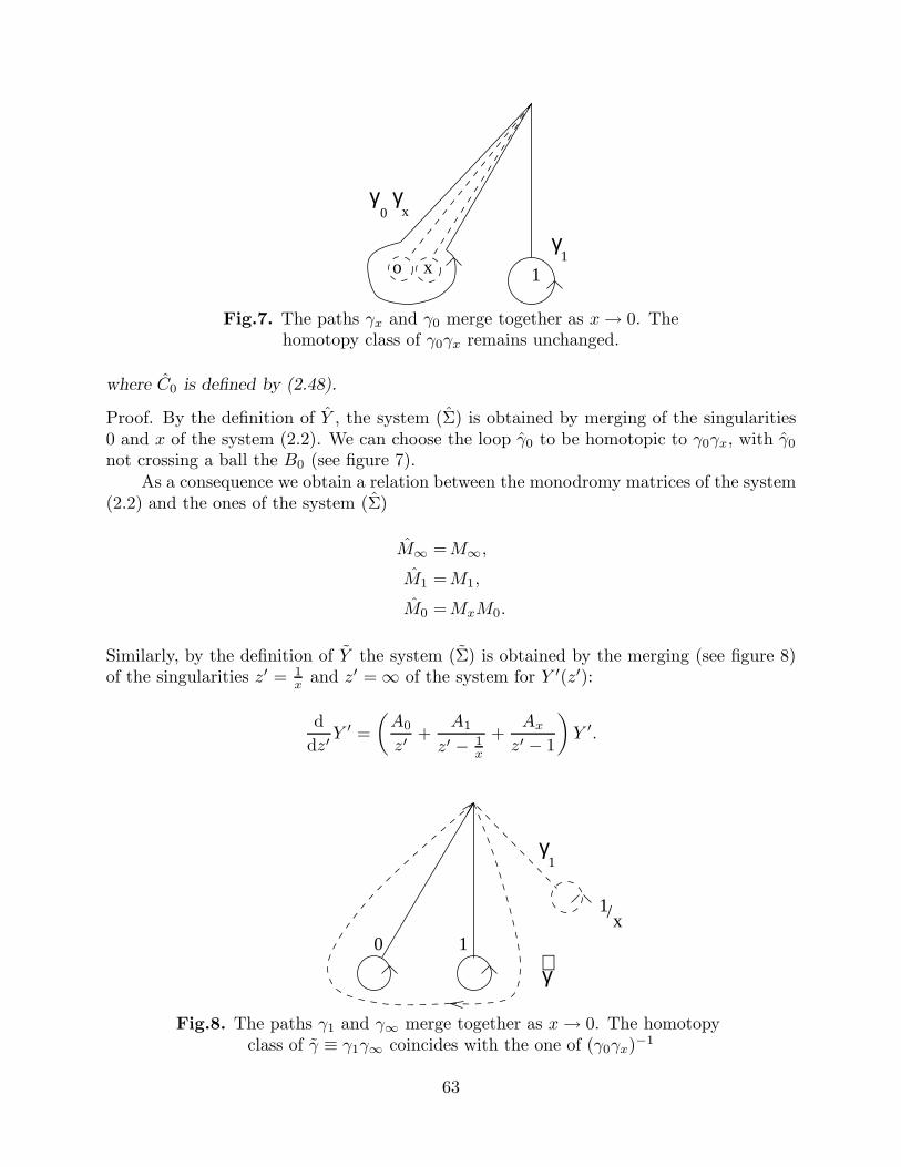
xo 1

γ

γ γ0 x

1

Fig.7. The paths γx and γ0 merge together as x→ 0. Thehomotopy class of γ0γx remains unchanged.

where C0 is defined by (2.48).

Proof. By the definition of Y , the system (Σ) is obtained by merging of the singularities0 and x of the system (2.2). We can choose the loop γ0 to be homotopic to γ0γx, with γ0

not crossing a ball the B0 (see figure 7).As a consequence we obtain a relation between the monodromy matrices of the system

(2.2) and the ones of the system (Σ)

M∞ =M∞,

M1 =M1,

M0 =MxM0.

Similarly, by the definition of Y the system (Σ) is obtained by the merging (see figure 8)of the singularities z′ = 1

xand z′ = ∞ of the system for Y ′(z′):

d

dz′Y ′ =

(

A0

z′+

A1

z′ − 1x

+Ax

z′ − 1

)

Y ′.

0 1∼γ

1/x

γ1

Fig.8. The paths γ1 and γ∞ merge together as x→ 0. The homotopyclass of γ ≡ γ1γ∞ coincides with the one of (γ0γx)−1

63

So, in the basis Y , the monodromy matrices of (Σ) have the following form:

M∞ = C−10 M∞M1C0

M1 = C−10 MxC0,

M0 = C−10 M0C0.

The lemma is proved. QED

Now we want to compute the monodromy matrices Mi and Mi and the connectionmatrix C0. To this aim we have to solve the systems (Σ) and (Σ), namely we have to de-termine T and b. For σ0 6= 0, this can be done introducing a suitable gauge transformationof Y and Y such that the systems (Σ) and (Σ) are equivalent to a Gauss equation. Thecase σ0 = 0 will be treated later.

2.2.1. Reduction to the Gauss equation. First of all let us notice that both thesystems (Σ) and (Σ) have similar form. We want to reduce them, via a suitable gaugetransformation and a appropriate choice of the parameters α, β, γ, to systems of the form:

d

dzY (z, α, β, γ) =

(

B0

z+

B1

z − 1

)

Y (z, α, β, γ) (2.52)

where B0, B1 are some constant matrices with eigenvalues 1 − γ, 0 and γ − α − β − 1, 0

respectively and B0 +B1 = −(

α 00 β

)

.

Lemma 2.8. For α 6= β, the system (2.52) is uniquely determined, up to a diagonalconjugation

B0 → T−1B0T, B1 → T−1B1T, with T =

(

1 00 r

)

, r 6= 0. (2.53)

The entries b0ij and b1ij of the matrices B0 and B1 respectively, are given by the formulae

b011 =α(γ − 1 − β)

β − α, b022 =

−β(γ − 1 − α)

β − α, b111 =

−α(γ − 1 − α)

β − α, (2.54)

b122 =β(γ − 1 − β)

β − α, b012b

021 = b112b

121 =

−αβ(γ − 1 − β)(γ − 1 − α)

(β − α)2. (2.55)

The system (2.52) can be solved using the Gauss hypergeometric function. So, we cancompute its connection matrices via the Kummer relations (see [Luke]) of the hypergeo-metric functions.

Lemma 2.9. The solutions of (2.52) have the form Y =

(

y1

y2

)

, with y1 being an arbitrary

solution of the following Gauss equation:

z(1 − z)y′′1 + [c− (a+ b+ 1)z]y′1 − aby1 = 0 (2.56)

64

where a = α, b = β + 1, c = γ and y2 given by:

y2(z) = r−1 β − α

β(γ − β − 1)

{

z(z − 1)d

dzy1(z) +

[

αz +α(γ − β − 1)

β − α

]

y1(z)

}

(2.57)

where r = − (β−α)b012β(γ−β−1) .

Proof. After the gauge transformation:

Y (z, α, β, γ) = zb011(1 − z)b111U(z, α, β, γ),

one obtains from (2.52) the following Riemann equation for u1

u′′1 +

[

1 + b011 − b022z

+1 + b111 − b122

z − 1

]

u′1 −b011b

022

z2(z − 1)2u1 = 0.

Now u1 is related with the solution yG of the Gauss equation (2.56), with a = −b011 − b111,

b = 1 − b022 − b122, c = 1 − b011 − b022, via the relation u1 = z−b011(1 − z)−b111yG. As aconsequence, thanks to (2.54), (2.55), we obtain that y1 = yG and a = α+1, b = β, c = γ.y2 it is given by:

(

b012z

+b112z − 1

)

y2 = y′1 −(

b011z

+b111z − 1

)

y1

that gives the equation (2.57). QED

To reduce the systems (Σ) and (Σ) to the system (2.52) we need to diagonalize thematrices A0

1+Λ = −A∞ and Λ respectively and to perform a suitable gauge transform. We

need to introduce some notations. Denote Cα,β,γ0,1 the connection matrices of the system

(2.52). The matrices J0,1 are the Jordan normal forms of B0,1 and the matrices Gα,β,γ0,1

are such that Gα,β,γ0,1 J0,1

(

Gα,β,γ0,1

)−1

= B0,1. Then for the asymptotic behaviour of an

appropriate fundamental matrix Y (z, α, β, γ) of the system (2.52) we have

Y (z, α, β, γ) =

(

1 + O(1

z)

)

z−

(

α 00 β

)

z → ∞

= Gα,β,γ0 (1 + O(z)) zJ0Cα,β,γ

0 z → 0

= Gα,β,γ1 (1 + O(z − 1)) (z − 1)J1Cα,β,γ

1 z → 1.

Some further remarks on the notations: from now on all the quantities with the hat arereferred to the system (Σ) and all the quantities with the tilde to the system (Σ). Whenwe don’t put any hat or tilde, the formulae are true for both the systems. In otherwords, they hold true for the generic system (2.52); substituting all the quantities withthe correspondent hat or tilde ones, the formulae hold true for the systems (Σ) or (Σ)respectively.

65

We now choose the values of α, β, γ in relation with the eigenvalues of the matrices ofthe systems (Σ) and (Σ). Namely, for (Σ) we take

α =ϑ∞ − σ0

2, β = −ϑ∞ + σ0

2, γ = 1 − σ0, (2.58)

and for (Σ) we take:

α = −σ0

2, β =

σ0

2, γ = 1. (2.59)

With this choice of the values of α, β, γ, one has:

J0 =

(

1 − γ 00 0

)

, J0 =

(

0 10 0

)

, J1 = J1 =

(

0 10 0

)

.

Now we can reduce the systems (Σ) and (Σ) to the system (2.52) via the following gaugetransformations:

Y = zα+β

2 Y (z, α, β, γ), Y = Gα,β,γ0 Y (z, α, β, γ), (2.60)

where Gα,β,γ0 is such that

Λ − α+ β

2Id = Gα,β,γ

0

(

−α 00 −β

)

(Gα,β,γ0 )−1.

As a consequence the connection matrices of (2.52) are related to the ones of (Σ) and (Σ)by the following formulae:

G1 = Gα,β,γ1 , C1 = Cα,β,γ

1 , C0 = Gα,β,γ0 Cα,β,γ

0 (2.61)

G0,1 = Gα,β,γ0 Gα,β,γ

0,1 , C0,1 = Cα,β,γ0,1 (Gα,β,γ

0 )−1. (2.62)

2.2.2. Local behaviour of the solution of (2.52). The solutions of (2.56) aroundthe singular points 0, 1,∞ are known and one can compute y2 by (2.57). In this wayone obtains the local behaviour of the fundamental solution Y for z → 0, 1,∞, and onecan compute the connection matrices by the Kummer relations (which are the connectionformulae for the hypergeometric equation). The difference w.r.t. the situation of [Jim] isthat in our case the Gauss equation is degenerate, namely:

c− a− b = 0, c− a− b = 0, c = 1.

So, we have to consider the logarithmic solutions of the Gauss equation around z = 1for both the systems (Σ) and (Σ), and around z = 0 for (Σ); moreover, we shall use theextension of the Kummer relations to this logarithmic case (see [Nor]).

66

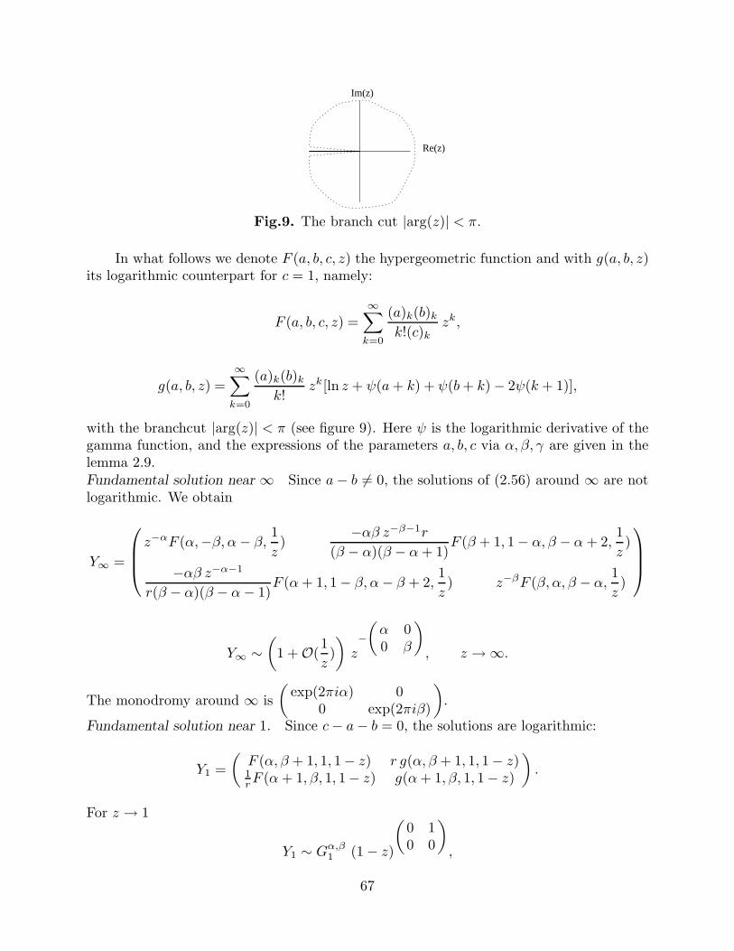
Re(z)

Im(z)

Fig.9. The branch cut |arg(z)| < π.

In what follows we denote F (a, b, c, z) the hypergeometric function and with g(a, b, z)its logarithmic counterpart for c = 1, namely:

F (a, b, c, z) =∞∑

k=0

(a)k(b)k

k!(c)k

zk,

g(a, b, z) =

∞∑

k=0

(a)k(b)k

k!zk[ln z + ψ(a+ k) + ψ(b+ k) − 2ψ(k + 1)],

with the branchcut |arg(z)| < π (see figure 9). Here ψ is the logarithmic derivative of thegamma function, and the expressions of the parameters a, b, c via α, β, γ are given in thelemma 2.9.Fundamental solution near ∞ Since a− b 6= 0, the solutions of (2.56) around ∞ are notlogarithmic. We obtain

Y∞ =

z−αF (α,−β, α− β,1

z)

−αβ z−β−1r

(β − α)(β − α+ 1)F (β + 1, 1 − α, β − α+ 2,

1

z)

−αβ z−α−1

r(β − α)(β − α− 1)F (α+ 1, 1 − β, α− β + 2,

1

z) z−βF (β, α, β − α,

1

z)

Y∞ ∼(

1 + O(1

z)

)

z−

(

α 00 β

)

, z → ∞.

The monodromy around ∞ is

(

exp(2πiα) 00 exp(2πiβ)

)

.

Fundamental solution near 1. Since c− a− b = 0, the solutions are logarithmic:

Y1 =

(

F (α, β + 1, 1, 1− z) r g(α, β + 1, 1, 1− z)1rF (α+ 1, β, 1, 1− z) g(α+ 1, β, 1, 1− z)

)

.

For z → 1

Y1 ∼ Gα,β1 (1 − z)

(

0 10 0

)

,

67

with

Gα,β1 =

(

1 r[ψ(α) + ψ(1 + β) − 2ψ(1)]1r

ψ(1 + α) + ψ(β) − 2ψ(1)

)

.

The monodromy around 1 is

(

1 2iπr0 1

)

.

Fundamental solution near 0. We have to distinguish the case (Σ), where the solutionsof (2.56) around 0 are not logarithmic, and the case (Σ), where c = 1 and the solutionsare logarithmic.

For (Σ) one has

Y0 =

− α

β−αz−α−βF (−β, 1 − α, 1 − α− β, z) r β

β−αF (α, β + 1, α+ β + 1, z)

− β

r(β−α)z−α−βF (1 − β,−α, 1 − α− β, z) α

β−αF (α+ 1, β, α+ β + 1, z)

.

For z → 0 it behaves like

Y0 ∼ Gα,β0 z

(

−α− β 00 0

)

where

Gα,β0 =

1

β − α

(−α r β

− βr

α

)

.

The monodromy around 0 is

(

exp(−2iπ(α+ β) 00 1

)

.

For (Σ) one has

Y0 =

(

F (α, 1 − α, 1, z) r g(α, 1 − α, 1, z)−1

rF (α+ 1,−α, 1, z) −g(α+ 1,−α, 1, z)

)

,

for z → 0 it behaves like

Y0 ∼ Gα0 z

(

0 10 0

)

with

Gα0 =

(

1 r[ψ(1 − α) + ψ(α) − 2ψ(1)]−1

r−ψ(1 + α) − ψ(−α) + 2ψ(1)

)

.

The monodromy around 0 is

(

1 2iπr0 1

)

.

2.2.3. Connection formulae. In order to compute the connection matrices we writeY∞ in the form:

Y∞ =

exp(−iπα)U(α, β + 1, z)−αβ exp(−iπ(β + 1))r

(β − α)(β − α+ 1)U(β + 1, α, z)

−αβ exp(−iπ(α+ 1))

r(β − α)(β − α− 1)U(α+ 1, β, z) exp(−iπβ)U(β, α+ 1, z)

68

where U(a, b, z) :=(

z−1eiπ)−a

F (a, 1− b, 1+a− b, 1z). For z such that |arg(z)| < 2π, there

are the following connection formulae:

U(a, b, z)∣

∣

z→1=− exp(iπa)Γ(1 + a− b)

Γ(a)Γ(1 − b)

{

[iπ + ψ(1 − b) − ψ(b)]F (a, b, 1, 1− z)+

g(a, b, 1, 1− z)}

,

U(a, 1 − a, z)∣

∣

z→0=

−Γ(2a)

Γ(a)2{[−iπ + ψ(a) − ψ(1 − a)]F (a, 1− a, 1, z) + g(a, 1− a, 1, z)} ,

U(a, b, z)∣

∣

z→0=

Γ(1 + a− b)Γ(1 − a− b)

Γ(1 − b)2F (a, b, a+ b, z) +

Γ(1 + a− b)Γ(a+ b− 1)

Γ(a)2·

· z1−a−bF (1 − b, 1 − a, 2 − a− b, z).

Using these relations we obtain the analytic continuation of Y∞ around 0 and 1, and bythe definition of the connection matrices

Y∞∣

∣

z→0,1= Y0,1C

α,β,γ0,1 ,

we obtain, by straightforward computations

Cα,β0 =

exp(iπβ)Γ(α+β)Γ(α−β+1)Γ(α)Γ(1+α)

−r exp(−iπα)Γ(α+β)Γ(1−α+β)

Γ(β)Γ(1+β)

1r

exp(−iπα)Γ(−α−β)Γ(α−β+1)

Γ(1−β)Γ(−β)− exp(−iπβ)Γ(−α−β)Γ(1−α+β)

Γ(−α)Γ(1−α)

,

Cα,β1 =

− Γ(α−β)

Γ(α)Γ(−β)[iπ + π cot(πα)] − Γ(−α+β)

Γ(−α)Γ(β)[iπ + π cot(πβ)]

−1r

Γ(α−β)

Γ(α)Γ(−β)− Γ(−α+β)

Γ(−α)Γ(β)

, (2.63)

Cα0 =

(

Γ(2α)Γ2(α) exp(−iπα)[iπ + π cot(πα)] r Γ(−2α)

Γ2(−α) exp(iπα)[π cot(πα) − iπ]

−1r

Γ(2α)Γ2(α) exp(−iπα) Γ(−2α)

Γ2(−α) exp(iπα)

)

, (2.64)

Cα1 =

(

−Γ(2α)Γ2(α)

[iπ − π cot(πα)] −r Γ(−2α)Γ2(−α)

[π cot(πα) + iπ]

−1r

Γ(2α)Γ2(α) −Γ(−2α)

Γ2(−α)

)

.

Now we have to compute the monodromy matrices in the basis Y∞. Using the formulae(2.51), (2.61) and (2.62) we have

M1 = (Cα,β1 )−1

(

1 2πir0 1

)

Cα,β1 , M0,x = (Cα,β

0 )−1(Cα0,1)

−1

(

1 2πir0 1

)

Cα0,1C

α,β0 .

Now we put

r =− exp[−iπ(α− β)]Γ(α− β)Γ(β)Γ(−α)

Γ(β − α)Γ(−β)Γ(α)r

69

and

r =exp(−2iπα)Γ(2α)Γ(−α)2

Γ(−2α)Γ(α)2s.

In this way we immediately obtain the formula (2.40) for M1 and it turns out that

Cα,β0 = Dα,β · C

where C is given in the formula (2.44) and

Dα,β :=

(

exp(iπβ)Γ(β+α)Γ(1−β+α)αΓ(α)2 sin πα

0

0 − exp(−iπβ)Γ(−β−α)Γ(1+β−α)Γ(1−α)Γ(−α) sin πα

)

.

As a consequence, one has

CM0,xC−1 = (Dα,β)−1(Cα

0,1)−1

(

1 2πir0 1

)

Cα0,1D

α,β.

By straightforward computations one can easily check that, for

s = −exp(2iπβ)Γ(β + α)Γ(1 − β + α)Γ(1 − α)Γ(−α)

Γ(−β − α)Γ(1 + β − α)αΓ(α)2s

i.e. forr

r= − Γ(1 − σ0)

2Γ(σ0

2 )2

Γ(1 + σ0)2Γ(−σ0

2 )2Γ(1 + ϑ∞+σ0

2 )Γ(1 + −ϑ∞+σ0

2 )

Γ(1 + ϑ∞−σ0

2 )Γ(1 − ϑ∞+σ0

2 )

s

r,

the formulae (2.41), (2.42) hold true.To conclude the proof we have to prove the relation (2.43), namely we want to prove

that rr

= − 14a0

2µ+σ0

2µ−σ0. To this aim we compute the matrices A0

0,1,x and Λ and then the

asymptotic behaviour of y in terms of σ0 and r. To compute the matrices A00,1,x and Λ we

observe that, thanks to the gauges (2.60),

A01 = B1, Λ = B0 +

α+ β

21, A0

0,x = Gα,β0 B0,1(G

α,β0 )−1.

First of all one has to compute the B0,1:

B0 = Gα,β,γ0 J0 (Gα,β,γ

0 )−1, B1 = Gα,β,γ1 J1 (Gα,β,γ

1 )−1

then

B0 =1

β − α

(

α2 −rαβαβr

−β2

)

, B1 =αβ

β − α

(

−1 r−1

r1

)

,

and

B1 =α

2

(

−1 r−1

r1

)

, B0 = − α2

(

1 r−1

r−1

)

.

70

It is then obvious that, referring to (2.49) and (2.50), b = r, T = Gα,β0 . Using the formula

(2.18),

y(x) ∼ − r(σ0 + 2µ)

4r(2µ− σ0)x1−σ0 .

This proves the formula (2.43) and concludes the proof of the theorem, in the case σ0 6= 0.For completeness we write here the result for the matrices A0

0,1,x and Λ:

Λ =1

4ϑ∞

(−ϑ∞2 − σ20 (−ϑ∞2 + σ2

0)r−σ2

0+ϑ∞

2

rϑ∞

2 + σ20

)

, A01 =

ϑ∞2 − σ2

0

4ϑ∞

(

−1 r−1

r1

)

,

A00 = 1

8θ

θ2 − σ20

2(r

r+r

r) − θ2 − σ2

0

1

r

(

−(θ − σ0)2r

2r− (θ + σ0)

2r

2r+ θ2 − σ2

0

)

r

(

(θ − σ0)2r

2r+

(θ + σ0)2r

2r+ σ2

0 − θ2

)

−θ2 − σ2

0

2(r

r+r

r) + θ2 + σ2

0

A0x = 1

8ϑ∞

σ20 − ϑ∞

2

2(r

r+r

r) − ϑ∞

2 − σ20

1

r

(

(ϑ∞ − σ0)2r

2r+

(ϑ∞ + σ0)2r

2r+ ϑ∞

2 − σ20

)

r

(

−(ϑ∞ − σ0)2r

2r− (ϑ∞ + σ0)

2r

2r+ σ2

0 − ϑ∞2

)

ϑ∞2 − σ2

0

2(r

r+r

r) + ϑ∞

2 + σ20

.

2.2.4. Case σ0 = 0. In this case the solution of the system (Σ) has logarithmic behaviouraround 0. Moreover, as seen before, it has a logarithmic behaviour around 1. For thissystem we can use all the formulae derived for (Σ), substituting α by α. The treatment ofthe (Σ), is even easier. Ideed in this case Λ has zero eigenvalues and it is straightforwardto solve the system (2.52) exactly. In fact in this case we have

B0 + B1 =

(

0 10 0

)

, det Bi = TrBi = 0, i = 0, 1.

Then the matrices B0 and B1 are uniquely determined up to an arbitrary parameter s:

B0 =

(

0 s0 0

)

, B1 =

(

0 1 − s0 0

)

,

and we can solve the differential equation (2.52) explicitly:

Y =

(

1 s log z + (1 − s) log(z − 1)0 1

)

.

71

The solution Y has the following asymptotic behaviour near the singular points:

Y =

(

1 + O(

1

z

))

zJ , as z → ∞,

= G0 (1 + O(z)) zJ C0, as z → 0,

= G1 (1 + O(z − 1)) (z − 1)J C1 as z → 1,

where J =

(

0 10 0

)

. It’s easy to verify that

C0 =

(

1 00 s

)

, C1 =

(

1 00 1 − s

)

, G0 =

(

1 00 1

s

)

, G1 =

(

1 00 1

1−s

)

.

As a consequence the monodromy matrices of the system (2.52) are

M0 =

(

1 2πis0 1

)

, M1 =

(

1 2πi(1 − s)0 1

)

. (2.65)

The correspondent monodromy matrices of the full system (2.2) are given by:

M1 = (Cα1 )−1

(

1 2iπr0 1

)

Cα1 , and M0,x = (Cα

0 )−1M0,1Cα0 ,

where

Cα0 =

(

πΓ(2α)Γ2(α) sin πα

r πΓ(−2α)Γ2(−α) sinπα

−1r

Γ(2α) exp(−iπα)Γ2(α)

Γ(−2α) exp(iπα)Γ2(−α)

)

,

and

Cα1 =

(

πΓ(2α) exp(−iπα)Γ2(α) sinπα

−r πΓ(−2α) exp(iπα)Γ2(−α) sin πα

−1r

Γ(2α)Γ2(α) −Γ(−2α)

Γ2(−α)

)

.

We observe thatCα

0,1 = C0,1Dα,

where

Dα =

(

πΓ(2α) exp(−iπα)Γ(α)2 sin πα

0

0 −Γ(−2α)Γ(−α)2

)

,

and

C0 =

(

exp(iπα) −rπsin πα

− sin παπr

exp(iπα)

)

, C1 =

(

1 rπ exp(iπα)sin πα

− sinπα exp(iπα)πr

1

)

.

We can factor out the diagonal matrix Dα in (2.65), and take r = 1. In this way, we obtainthe formulae (2.45), (2.46), (2.47). The asymptotic behaviour of y(x) can be computed asbefore. For σ0 = 0 we obtain:

y ∼ a0x for a0 = s.

72

This concludes the proof of the theorem.

2.2.5. The asymptotic behaviour near 1,∞ and the monodromy data. We canprove the analogue of Theorem 2.2 near 1 and ∞. Namely, for any pair of values (a1, σ1)there exists a unique branch of the solution of PVIµ with the asymptotic behaviour

y(x) ∼ 1 − a1x1−σ1 as x→ 1. (2.66)

It is possible to parameterize the monodromy matrices as in Theorem 2.2 substituting σ0

with σ1 and M0 with M1 and vice-versa. Analogously, for any pair of values (a∞, σ∞)there exists a unique branch of the solution of (PVI) with the asymptotic behaviour

y(x) ∼ a∞xσ∞ as x→ ∞, (2.67)

and it is possible to parameterize the monodromy matrices as before, substituting σ0 withσ∞ and applying the braid β2 to the monodromy matrices.

2.3. From the local asymptotic behaviour to the global one.

In this section we prove Theorem 2.1 which gives the asymptotic behaviour of thebranches of the solutions in terms of the triplets (x0, x1, x∞).

Lemma 2.10. For the solution y(0)(x) of PVIµ behaving as

y(0)(x) = a0x1−σ0 (1 + O(xε)) as x→ 0,

with 0 ≤ σ0 < 1 and a0 6= 0, a0 6= 1 for σ0 = 0, the canonical form (1.20) of the

monodromy matrices M(0)0 ,M

(0)x ,M

(0)1 given by (2.42), (2.41), (2.40), or (2.46), (2.47),

(2.45) for σ0 = 0, is the following:

M0 =

(

1 −x(0)0

0 1

)

, Mx =

(

1 0x

(0)0 1

)

, M1 =

1 +x(0)1 x(0)

∞

x(0)0

− (x(0)1 )2

x(0)0

(x(0)∞

)2

x(0)0

1 − x(0)1 x(0)

∞

x(0)0

,

where the triple (x(0)0 , x

(0)1 , x

(0)∞ ) is defined, up to equivalence, by the following formulae,

for σ0 6= 0:

x(0)0 = −2 sin

πσ0

2,

x(0)1 = −

√

2(cosπσ0 − cos 2πµ)sin πφ

2

sin πσ0

2

,

x(0)∞ = −

√

2(cosπσ0 − cos 2πµ)cos π(σ0+φ)

2

sin πσ0

2

,

(2.68)

with φ given by

eiπφ =1

4a0

σ0 + 2µ

σ0 − 2µ

Γ(1 + σ0)2Γ(1 − σ0

2 )2Γ(1 + µ− σ0

2 )Γ(1 − µ− σ0

2 )

Γ(1 − σ0)2Γ(1 + σ0

2)2Γ(1 + µ+ σ0

2)Γ(1 − µ+ σ0

2), (2.69)

73

and for σ0 = 0:

x(0)0 = 0,

x(0)1 = −| sinπµ|

√1 − a0

x(0)∞ = −| sinπµ|√a0.

(2.70)

The proof of this lemma can be obtained by straightforward computations, using

the algorithm of lemma 1.5. Similar formulae for the parameters (x(1)0 , x

(1)1 , x

(1)∞ ) and

(x(∞)0 , x

(∞)1 , x

(∞)∞ ) can be obtained respectively starting from a solution y(1)(x) of PVIµ

behaving as

y(1)(x) = 1 − a1(1 − x)1−σ1 (1 + O(1 − x)ε) as x→ 1,

or from another solution y(∞)(x) of PVIµ behaving as

y(∞)(x) = a∞xσ∞

(

1 + O(1

xε)

)

as x→ ∞.

So, given an admissible triple (x0, x1, x∞), with xi ∈ lR, |xi| < 2 for i = 0, 1,∞, we choosethe parameters µ, (a0, σ0), (a1, σ1) and (a∞, σ∞) in such a way that (2.8) is satisfied and

x(0)i = x

(1)i = x

(∞)i = xi, for i = 0, 1,∞.

Using the explicit formulae (2.68), (2.69) for x0 6= 0, we derive the expressions (2.10),(2.11). Similarly, using (2.70) for x0 = 0 we derive the expression (2.12). In the same way,we derive the analogous expressions for (a1, σ1) and (a∞, σ∞). The three correspondentbranches y(0)(x), y(1)(x), y(∞)(x) of solutions of PVIµ, with µ given by (2.8) must coincide.In fact, the associated auxiliary Fuchsian systems have the same, modulo diagonal con-jugation, monodromy matrices. This proves the existence of a solution of PVIµ with theasymptotic behaviour (2.1), with the indices given by (2.9) and the coefficients specifiedas above, for any admissible triple (x0, x1, x∞), with xi ∈ lR, |xi| < 2 for i = 0, 1,∞. Theuniqueness of such a branch follows from theorem 1.3.

Conversely, for any such a solution we obtain an admissible triple (x0, x1, x∞) =

(x(0)0 , x

(0)1 , x

(0)∞ ) = (x

(1)0 , x

(1)1 , x

(1)∞ ) = (x

(∞)0 , x

(∞)1 , x

(∞)∞ ), using the formulae (2.68), (2.69)

or (2.70) and their analogies. Let us prove that the numbers (x0, x1, x∞) are real andsatisfy |xi| < 2 for i = 0, 1,∞. Indeed, from the definition of the parameters, it follows:

(x(0)0 )2 = 4 sin2 πσ0, (x

(1)1 )2 = 4 sin2 πσ1, (x

(∞)∞ )2 = 4 sin2 πσ∞.

This proves that our construction covers, for real µ, all the solutions of PVIµ with criticalbehaviour of algebraic type.

Finally, using corollary 1.5, we infer that the class of solutions of PVIµ, with realµ, having critical behaviour of algebraic type is invariant with respect to the analyticcontinuation. The law of transformation of the critical indices l0, l1, l∞ of the expansions(2.1), is described by theorem 1.5.

74

2.4. The complete list of algebraic solutions

We summarize the results of this paper in the following

Classification Theorem. Any algebraic solution of the equation PVIµ with 2µ 6∈ ZZ isequivalent, in the sense of symmetries (1.22), (1.23), (1.24) to one of the five solutions(A3), (B3), (H3), (H3)

′, (H3)′′ below.

We already know that the classes of equivalent algebraic solutions are labelled bythe five regular polyhedra and star-polyhedra in the three-dimensional space. We willconstruct representatives in these classes for the following values of the parameter µ

µ = −1

4, −1

3, −2

5, −1

5, −1

3.

The correspondent algebraic solutions will have 4, 3, 10, 10, 18 branches respectively. Re-call that these are the lenghts of the orbits (1.33), (1.34), (1.35), (1.36), (1.37) respectivelywith respect to the action of the pure braid group (see remark 1.11 above). We give nowthe explicit formulae for the solutions with brief explanations of the derivations of them.

Tetrahedron. We have (x0, x1, x∞) = (−1, 0,−1), then µ = −14 and

y =(s− 1)2(1 + 3s)(9s2 − 5)2

(1 + s)(25 − 207s2 + 1539s4 + 243s6),

x =(s− 1)3(1 + 3s)

(s+ 1)3(1 − 3s).

(A3)

(We present the solution in the parametric form). The monodromy matrices, in thecanonical form (1.20), are:

M0 =

(

1 10 1

)

Mx =

(

1 0−1 1

)

M1 =

(

1 01 1

)

.

This solution was found in [Dub] in the implicit form (E.29). This was also obtained,independently, by N. Hitchin (see [Hit2]). To reduce (E.29) to the above form, wehave to solve the cubic equation (E.29 b) with the substitution:

t =32(1 − 18s2 + 81s4)

27(1 + 9s2 + 27s4 + 27s6).

Then the three roots of (E.29 b) are:

ω1 =13 − 66s2 − 27s4

3(1 + 3s2)2,

ω2,3 =−5 + 42s2 ± 144s3 + 27s4

3(1 + 3s2)2.

75

Cube. We have (x0, x1, x∞) = (−1, 0,−√

2) and µ = −13 . The solution

y =(2 − s)2(1 + s)

(2 + s)(5s4 − 10s2 + 9),

x =(2 − s)2(1 + s)

(2 + s)2(1 − s),

(B3)

was obtained in [Dub]. The canonical form for the monodromy matrices is:

M0 =

(

1 10 1

)

Mx =

(

1 0−1 1

)

M1 =

(

1 0−2 1

)

.

Coxeter group W(H3), of symmetries of icosahedron. We have three possiblechoices of the point (x0, x1, x∞) which lead to three different solutions.

Icosahedron. The orbit (1.35) corresponds to the standard triple of reflections for

the icosahedron. (x0, x1, x∞) = (0,−1,−1+√

52 ), then µ = −2

5 and

y =(s− 1)2(1 + 3s)2(−1 + 4s+ s2)(7 − 108s2 + 314s4 − 588s6 + 119s8)2

(1 + s)3(−1 + 3s)P (s)

x =(−1 + s)

5(1 + 3 s)

3 (−1 + 4 s+ s2)

(1 + s)5(−1 + 3 s)

3(−1 − 4 s+ s2)

,

(H3)

with

P (s) =49 − 2133s2 + 34308s4 − 259044s6 + 16422878s8 − 7616646s10 + 13758708s12

+ 5963724s14 − 719271s16 + 42483s18.

The canonical form for the monodromy matrices is:

M0 =

(

1 10 1

)

Mx =

(

1 0−1 1

)

M1 =

(

1 0−3−

√5

2 1

)

.

The above solution was already obtained in [Dub] in the implicit form (E.33). Theabove explicit formula can be obtained solving (E.33 b) in the form:

t =(1 − 4s− s2)(−1 − 4s+ s2)(−1 + 5s2)

(1 + 3s2)3

ω1 =25 − 585 s2 + 3530 s4 − 6690 s6 − 3955 s8 + 507 s10

(1 + 3 s2)5

ω2 =−7 + 215 s2 − 1910 s4 − 4096 s5 + 5150 s6 + 20480 s7 + 6125 s8 − 357 s10

(1 + 3 s2)5

ω3 =−7 + 215 s2 − 1910 s4 + 4096 s5 + 5150 s6 − 20480 s7 + 6125 s8 − 357 s10

(1 + 3 s2)5.

76

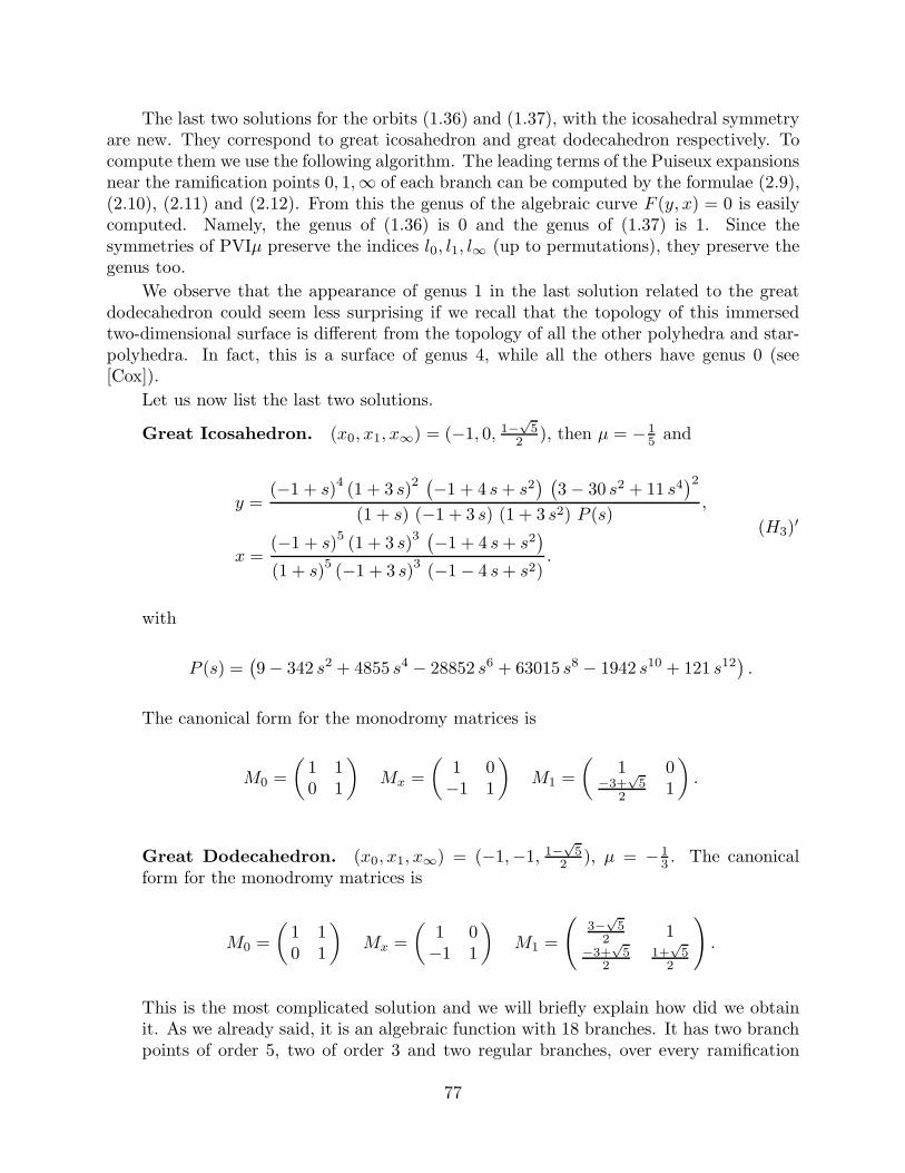
The last two solutions for the orbits (1.36) and (1.37), with the icosahedral symmetryare new. They correspond to great icosahedron and great dodecahedron respectively. Tocompute them we use the following algorithm. The leading terms of the Puiseux expansionsnear the ramification points 0, 1,∞ of each branch can be computed by the formulae (2.9),(2.10), (2.11) and (2.12). From this the genus of the algebraic curve F (y, x) = 0 is easilycomputed. Namely, the genus of (1.36) is 0 and the genus of (1.37) is 1. Since thesymmetries of PVIµ preserve the indices l0, l1, l∞ (up to permutations), they preserve thegenus too.

We observe that the appearance of genus 1 in the last solution related to the greatdodecahedron could seem less surprising if we recall that the topology of this immersedtwo-dimensional surface is different from the topology of all the other polyhedra and star-polyhedra. In fact, this is a surface of genus 4, while all the others have genus 0 (see[Cox]).

Let us now list the last two solutions.

Great Icosahedron. (x0, x1, x∞) = (−1, 0, 1−√

52

), then µ = −15

and

y =(−1 + s)

4(1 + 3 s)

2 (−1 + 4 s+ s2) (

3 − 30 s2 + 11 s4)2

(1 + s) (−1 + 3 s) (1 + 3 s2) P (s),

x =(−1 + s)

5(1 + 3 s)

3 (−1 + 4 s+ s2)

(1 + s)5(−1 + 3 s)

3(−1 − 4 s+ s2)

.

(H3)′

with

P (s) =(

9 − 342 s2 + 4855 s4 − 28852 s6 + 63015 s8 − 1942 s10 + 121 s12)

.

The canonical form for the monodromy matrices is

M0 =

(

1 10 1

)

Mx =

(

1 0−1 1

)

M1 =

(

1 0−3+

√5

21

)

.

Great Dodecahedron. (x0, x1, x∞) = (−1,−1, 1−√

52 ), µ = −1

3 . The canonicalform for the monodromy matrices is

M0 =

(

1 10 1

)

Mx =

(

1 0−1 1

)

M1 =

(

3−√

52 1

−3+√

52

1+√

52

)

.

This is the most complicated solution and we will briefly explain how did we obtainit. As we already said, it is an algebraic function with 18 branches. It has two branchpoints of order 5, two of order 3 and two regular branches, over every ramification

77

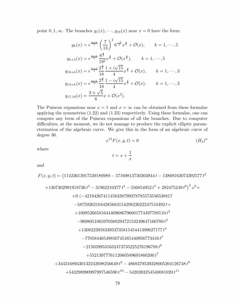
point 0, 1,∞. The branches y1(x), · · · , y18(x) near x = 0 have the form:

yk(x) = e2πik

5

(

7

13

)2

6−25 x

45 + O(x), k = 1, · · · , 5

yk+5(x) = e2πik

56

45

192x

25 + O(x

45 ), k = 1, · · · , 5

y10+k(x) = e2πik

32

23

18

1 + i√

15

4x

23 + O(x), k = 1, · · · , 3

y13+k(x) = e2πik

32

23

18

1 − i√

15

4x

23 + O(x), k = 1, · · · , 3

y17,18(x) =3 ±

√5

6x+ O(x2).

The Puiseux expansions near x = 1 and x = ∞ can be obtained from these formulaeapplying the symmetries (1.22) and (1.23) respectively. Using these formulae, one cancompute any term of the Puiseux expansions of all the branches. Due to computerdifficulties, at the moment, we do not manage to produce the explicit elliptic param-eterization of the algebraic curve. We give this in the form of an algebraic curve ofdegree 36.

x15F (x, y, t) = 0 (H3)′′

where

t = x+1

x

and

F (x, y, t) =(

11423613917539180989− 57169813730203944 t− 13869163074392577 t2

+1307302991918736 t3 − 31962210377 t4 − 556854952 t5 + 282475249 t6)2x9+

+9 (−42194267411458338799378785573556538817

−58759262104428568315429822622247510492 t+

+10095266581644469686796601774497789110 t2

−969805106597038829472153249647160780 t3

+13082239583395373581545441399627177 t4

−77058446549850745165440956773416 t5

−2150599531632473735225276196788 t6

+5521397776112060589691860200 t7

+34431689430132242698256649 t8 − 4868379539328005204126748 t9

+543298990997997546590 t10 − 5420393254540081020 t11

78

−79792266297612001 t12)

x8 (1 + x) y

+3 (1958540422461728364360419152068949457061

−2209393132972329408615760780334959957197 t

+3730909713982979160856372675878664915614 t2

−998456940153012666787445238400320871842 t3

+127635631698846877473536225998246411623 t4

−1482254497297246657880332587875322027 t5

+8847488219466307166390055942913100 t6

+115442527212405524632938663371228 t7

−1429542565820801871766655325509 t8

+7631245862019705473945545029 t9

+215859931310548879418863190 t10

−61369918621176379581242 t11

+443864075501101414537 t12

+239376798892836003 t13)

x8 y2

+8 (−14176454404869485146893293606614356611775

+28055900200716580071561317517835005937542 t

−22805214425386778204880821526748969126548 t2

+7203824414325261553629527716660045847442 t3

−941980967212371956151450075677431178469 t4

+8038149376577574092957422850094452382 t5

−22951481031624768208910085230213950 t6

−1567265072303229457696028497735362 t7

+17710721122570843039502588273105 t8

−100631536944878626686735036764 t9

−513222963217440801801106854 t10

+346131811374226777113368 t11

−1385596068253512936373 t12)

x7 (1 + x) y3

+6 (372245126038285018174621123839906354129684

79

−538123164074188598920246979212739683700019 t

+148097514409311992531878851512796911164392 t2

+131183971273631981690818920653550831952470 t3

−81255871706326021946002239342890704787124 t4

+13496764871847929345618085983834973142347 t5

−77522788387610267024773351181536807752 t6

−15773276759106249673670395386220524 t7

+43306225979803766149728090033557588 t8

−398429371182004923439978792917533 t9

+1762391142835398582269106251136 t10

+2388970787440139757429804470 t11

−3439831965306734927530580 t12

+6227088023782555081845 t13)

x7 y4

+6 (−1723593607166532080927038166074395946035900

+2040599178888751273951239802196511605636025 t

+233403452055579960658996997839662220718652 t2

−1266443503829326206558682114543567079698662 t3

+601472177228487289796456276889218593842200 t4

−90437995682218432847116536290883275511849 t5

+312726298388429638276816726813440288752 t6

+2550025722128829156352333577788952604 t7

−575104019542617989271403929336386084 t8

+4033434111720024901257683928676919 t9

−12117519775974826925705049828908 t10

−6556200250126220600244219830 t11

+14241314959493049268655304 t12

−9850799841945252913527 t13)

x6 (1 + x) y5

+2 (21644465131825357400382632120971734649857264

+1609281090760898028021044308156991213714259 t

80

−38819578264561008264384235926474662382590097 t2

+19461702669444598007359556763777303231431634 t3

+6809228919729818789589103927528063675916654 t4

−6502005871163632747227392004794985000703103 t5

+1176880351448958476049654953342289787508545 t6

−2305666451065939258487468463173953769764 t7

−66480299243646643579685794767909280748 t8

+15241200180683229312383060139285323669 t9

−78386104021612006912908252437015263 t10

+148880803913659745854808576095474 t11

+57461755817453559455002717038 t12

−103978838096755580164874073 t13

+22079893897296692642367 t14)

x6 y6

+12 (−3846090734682844350682028823106084687428444

−6334186503545807261781842904989156398103475 t

+13149149531444644750567430723972640952739601 t2

−833478059474840476986699901359926517619482 t3

−6957568559854570720866520753764257206265698 t4

+3704223179468379920674190362976879513996499 t5

−576109607175627912516018268715191958362489 t6

+449528751470785721434087640482632944192 t7

+97703132604175842587572789513022822852 t8

−16011119124352462144696375400709770865 t9

+57470033726311385832789992330535883 t10

−64186326557416461737056084783958 t11

−26094692352698228396829172726 t12

+25456979816863844482106097 t13

−1051423518918890125827 t14)

x5 (1 + x) y7

+3 (10610560214390717981593236262575236159801442

81

+111851425974428655491946571184648885748780846 t

−46715489836280837819492546495478177251546881 t2

−139030514021835704781706562226557058780091068 t3

+91919803393449431080407081029445741045516160 t4

+17286168898942635534811373112001322602942242 t5

−24220067368877156108293128216367359106738667 t6

+4637848726272650440828320863095758089676600 t7

−768878602349792937649689712426759282462 t8

−1741702208080601219941076960674171058190 t9

+291817792658031512381548036217335383393 t10

−703979549232767832584811827025318204 t11

+431869052449224832223544125220252 t12

+211026301709949401515207349982 t13

−88672767468343194407328645 t14)

x5 y8

+(29516093700614758561713684532397059536112914

−250427363718702318175164789552712875171021018 t

−276026230387316277405019906885146213095909789 t2

+798207668051094993868151955635553085940964248 t3

−344467523172443772269951999752021715572380244 t4

−120301086904813944940738235485125501727252554 t5

+109511261517293051818507102282993534830623481 t6

−19194080365623650515069714757340701033233072 t7

−51032394918091643798626435084286655402518 t8

+23520399409116636731567242035209841281394 t9

−2981630391452674856104059990243312091171 t10

+4599349671236813290177817558881705144 t11

−1416023622121443571963532624008680 t12

−884464824710945312016748613390 t13

+126470477973158698785100695 t14)

x4 (1 + x) y9

82

+3 (−10911639347758887707980330460476045164474906

−58595420545899882777261835025201788418411880 t

+510148671470006459933001332369933260295921507 t2

−421411310692898883818707378130970229534690273 t3

−167152535194408490298020642999503515413037404 t4

+259430867087315198025819011038004422708530022 t5

−46562493376530130089912033636689480134093531 t6

−21317412351831533402564088853511437604716591 t7

+5998321070650622801147765820299240777440702 t8

+42318724644239526363080933921378429784628 t9

−20025402467700581457477461594500061379211 t10

+2543243908066676381203685445622311376505 t11

−2382710944926354080442398446589552744 t12

+326767340108407733203130499898126 t13

+276491632581630260746191363123 t14

−8431365198210579919006713 t15)

x4 y10

+12 (−8733106988589310312964985955814462819079774

+64016502559572741731505856556403573520814046 t

−144735875200699985710584864792377620711111027 t2

+66707682241185015299381142924382044312819100 t3

+73079504596828994404469155513764487920535332 t4

−75764221368814908722894464652763782420369670 t5

+18144429124108777614777763808360976174204563 t6

+1935278311931502378271609920389021155764328 t7

−842229927380965714885405569219684268010166 t8

−43576284807293907660657241391770657495742 t9

+12197493655076249609592887507484958732619 t10

−1236906021392508491488029828633988502116 t11

+656542960338462752927669545849000176 t12

83

−33306604264547610372382676649434 t13

−41617303783672454910317327355 t14)

x3 (1 + x) y11

+2 (187554318014748213259275472412247634165779260

−762602529289184570716467664651505597594612711 t

+781137281074558579579982041608982979326338521 t2

+609916709974782293997005108542677011211842354 t3

−1300509731487820027375772452301766352965003310 t4

+495021556835245340779707559257082787835603199 t5

+115214340026017185187174532535570472667840767 t6

−93151202230256791649185399844658098150754584 t7

+7202343146876999296118334182261935450026080 t8

+1570014403002611359784317587694467895480399 t9

+371422610102654444897802704145750294582991 t10

−107776513895628817503345944747365689465454 t11

+10941070332070115448154615812894796283346 t12

−3005301616251624310474021462023025751 t13

+41932897601387821985740913526761 t14

+87168052345572726428101766292 t15)

x3 y12

+6 (−49769698820686378083743112964571467299790844

+144208424244836145109900273916270122534480379 t

−31061701177281181816778329394184658654578125 t2

−316115877280896274823885457480018099381675270 t3

+413355491574586200245516861333774692564805758 t4

−189323246544195194714568800051070616915145871 t5

+16358105769812410561563772201680559507177601 t6

+10699064629034472787428641330738981639504716 t7

−2410111354335748769859016926649172233001216 t8

+411171528032730820725099829153187243925077 t9

−226789949801107593485509158636442297272707 t10

84

+47843156588060602804351104035547186862994 t11

−4050842729096500910242692387785686802242 t12

+503056665812777017090193080924335791 t13

−1358120473689033753999092690625 t14

−4470156530542191098877013656 t15)

x2 (1 + x) y13

+6 (40840375974497844675523416705994772589613816

−31065278771086485580585566101107070670979537 t

−256058709793754221748465779158452450846012816 t2

+559068508134217391316137877579221486889948317 t3

−405356674135473476033247305191846353227354396 t4

+56661024338479719866449660305901198060970619 t5

+64125926679095609696574105582575413252584004 t6

−28890521413485617192612359619257982301215223 t7

+2839341861289460260556040613235064311172368 t8

+465313317652398071330581978147640308517821 t9

−351597845897601623389761113030041346811064 t10

+179321665024113431049966683538039741491991 t11

−39080763389941286051140782872898013637420 t12

+3329327789375495478533443619894892092425 t13

−149553232132910627041355116122361020 t14

+205192601853360299747062918515 t15)

x2 y14

+4 (−5628131126860710389875035169789649454420876

−78804574894375995596657603789677394324984101 t

+352860279249727357643015437757245513637138672 t2

−564941261129218367227412931528430799748606546 t3

+430939089346630550106464017811753376858010640 t4

−148284188482685309994113608598302973692022739 t5

+4873973943047627527185771161170310871611116 t6

+10181461701693419091610691800269773692583228 t7

85

−1226684412907984419281022032089194096771900 t8

−1114701349894370233505605371103641055314707 t9

+706698148832598485833137372995728746006888 t10

−230885597278675059768074093486733449982986 t11

+40110760213781966306595755424591426952408 t12

−2944406938738808019234484282441173992613 t13

+29909989810256194655311832623132956 t14)

x (1 + x) y15

+3 (−19345311524103689299806429866595584344434933

+165880840018062517894524148661179410853072546 t

−433975351186661527899190510419861031681577223 t2

+515516306674309051714096086492072331808918060 t3

−283562876761607595979024343783955270990852289 t4

+35089717870652037166528865782071242284918734 t5

+33297928990127187049831304457387943687578909 t6

−12917764244851664872827620472556082803226856 t7

−266713623245328356955979252488258143292463 t8

+555900198844440351814987030522263162652334 t9

+344809125199575823496923125385565831315595 t10

−325689072459807008457121908075371991483716 t11

+117388439783020206894897144460070846332949 t12

−21123688072686368568170196496753937437182 t13

+1569161588742434760282235480090100082255 t14)

x y16

+3 (9783299760488948030219433006083570296689357

−59321119347918543659930676521984384042169430 t

+141416477837529651726686264572772822193430055 t2

−177096809878289456793903796377476455257673500 t3

+127907586479651422318564410835908192786763365 t4

−54372658309139640733439296021048049726746698 t5

+13488394375983259178386269031077826541323679 t6

86

−2113244794203694376441274534558687456380488 t7

+141785257824097311610019381070069013792095 t8

+316821091130460893567937727374441119017078 t9

−305480360931755555721215775431316200256739 t10

+142141070595224470100170760768533902542116 t11

−38457837145846954116338584809621985652097 t12

+5806436836462494743682658146129894324810 t13

−380650359326333515862984779019865187923 t14)

(1 + x) y17

+(−10524240525647109159259219575804205851284241

+54473554541130948618895564303322618142908415 t

−116506041709060140591221129409148683447467665 t2

+134582692171688928175407226575844795641654895 t3

−91188532083602481766920967127844408926436405 t4

+36353592052137018784330858422674753425698363 t5

−7639385747972665348009342010125607135270845 t6

+93749989416978017153766638267237965058515 t7

+613514003480165484061014972915970847589645 t8

−277973572971202497026511206431230055671555 t9

+4186799108745525715968930085758736947197 t10

+68475809505229552273919737578535787115805 t11

−41025357958210023316522198089867194215575 t12

+12129433061687109251202289166065827342585 t13

−1903251796631667579314923895099325939615 t14

+126883453108777838620994926339955062641 t15)

y18.

87

BIBLIOGRAPHY

[AgLak] R.P. Agarwal and V. Lakshmikantham, Uniqueness and Non-uniqueness Criteria for

Ordinary Differential Equations, World Scientific (1993).

[Bat] H. Bateman and A. Erdelyi, Higher Transcendental Functions, Krieger Publishing,Florida (1981).

[Bir] J.S. Birman, Braids, Links, and Mapping Class Groups, Ann. Math. Stud. PrincetonUniversity (1975).

[Cox] H.S.M. Coxeter, Regular Polytopes, Macmillan Company New York (1963).

[Cro] W.J.R. Crosby, Problems and Solutions, Mounthly Amer. Math. (1946) 104-107.

[Dek] W. Dekkers, The Matrix of a Connection having Regular Singularities on a VectorBundle of Rank 2 on P 1(Cl ), Springer Lect. Notes Math. 712 (1979) 33-43.

[Dub] B. Dubrovin, Geometry of 2D Topological Field Theories, Springer Lect. Notes Math.

1620, (1995) 120-348.

[FlN] H. Flashka and A.C. Newell, Monodromy and Spectrum Preserving Deformations,Comm. Math. Phys. 76 (1980) 67-116.

[Fuchs] R. Fuchs, Uber Lineare Homogene Differentialgleichungen Zweiter Ordnung mit imdrei im Endrichen Gelegene Wesentlich Singularen Stellen, Math. Ann. 63 (1907)301-321.

[Gamb] B. Gambier, Sur les Equations Differentielles du Second Ordre et du Primier Degredont l’Integrale est a Points Critiques Fixes, Acta Math. 33, (1910) 1-55.

[Gar] R. Garnier, Sur des Equations Differentielles du Troisieme Ordre dont l’Integrale Gen-erale est Uniforme et sur una Classe d’Equations nouvelles d’Ordre Superieur dontl’Integrale Generale a ses Points Critiques Fixes, Ann. Sci. Ecole Norm. Sup. 3No.29 (1912) 1-126.

[Gor] P. Gordan, Uber endliche Gruppen linearer Transformationen einer Veranderlichen,Math. Ann. 12, 1877, 23-46.

[Hit] N.J. Hitchin, Twistor Spaces, Einstein Metrics and Isomonodromic Deformations, J.

Differential Geometry 42, No.1 July 1995 30-112.

[Hit1] N.J. Hitchin, Poncelet Polygons and the Painleve Transcendents, Geometry and Anal-

ysis, edited by Ramanan, Oxford University Press (1995) 151-185.

[Hit2] N.J. Hitchin, Talk at I.C.T.P. (Trieste) April 1993.

[IKSY] K. Iwasaki, H. Kimura, S. Shimomura, M. Yoshida, From Gauss to Painleve, a Modern

Theory for Special Functions, Chapter 4, Aspects of Mathematics, Vieweg (1991).

[Ince] E.L. Ince, Ordinary Differential Equations, Dover Publications, New York (1956).

[ItN] A.R. Its and V.Yu. Novokshenov, The Isomonodromic Deformation Method in theTheory of Painleve Equations, Springer Lect. Notes Math. 1191 (1986).

88

[Jim] M. Jimbo, Monodromy Problem and the Boundary Condition for some Painleve Equa-tions, Publ. RIMS 18 (1982), 1137-1161.

[JMU] M. Jimbo, T. Miwa and K. Ueno, Monodromy Preserving Deformation of the LinearOrdinary Differential Equations with Rational Coefficients I, II, Publ. RIMS 14 (1978)223-267, 15 (1979) 201-278.

[Kit] A.V. Kitaev, Rational Solutions of the Fifth Painleve Equation, Differential and In-

tegral Equations 7 (1994) no.3-4, 967-1000.

[Kr] L. Kronecker, J. de Math. 19 (1854) 177-192.

[Lak] V. Lakshmikantham and S. Leela, Differential and Integral Inequalities, AcademicPress New York (1969).

[Luka] N.A. Lukashevich, On the Theory of the Third Painleve Equation, Differ. Uravn. 3(1967) no.11, 1913-1923.

[Luke] L. Yu. Luke, Mathematical Functions and Their Approximations, Academic Press(1975).

[Mag] W. Magnus, Ring of Fricke Characters and Automorphism Groups of Free Groups,Math. Z. 170, (1980) 91-103.

[Mal] B. Malgrange, Sur les Deformations Isomonodromiques I, Singularites Regulieres,Seminaire de l’Ecole Normale Superieure 1979-1982, Progress in Mathematics 37,Birkhauser, Boston (1983) 401-426.

[Man] Yu.I. Manin, Sixth Painleve Equation, Universal Elliptic Curve and Mirror of P2,preprint al-geom/9605010 (1996).

[Ma] M. Mazzocco, Picard and Chazy Solutions to PVI Equation, preprint 1998.

[Miwa] T. Miwa, Painleve Property of Monodromy Preserving Deformation Equations andthe Analyticity of τ -function, Publ. RIMS, Kyoto Univ. 17 (1981) 703-721.

[Mur] Y. Murata, Classical Solutions of the Third Painleve Equation, Nagoya Math. J. 139(1995) 37-65.

[Mur1] Y. Murata, Rational Solutions of the Second and Fourth Painleve equations, Funk.

Ekvacioj 28, no.1 (1995).

[Nor] N.E. Norlund, The Logarithmic Solutions of the Hypergeometric equation, Mat. Fys.

Skr. Dan. Vid. Selsk. 2, no.5 (1963) 1-58.

[Ok] K. Okamoto, On the τ -Function of the Painleve Equations, Physica 2D (1981) 525-535.

[Ok1] K. Okamoto, Studies on the Painleve Equations I, Sixth Painleve Equation, Ann.

Mat. Pura Appl. 148 (1987) 337-381.

[Ok2] K. Okamoto, Painleve Equations and Dynkin Diagrams, Painleve Transcendents,

edited by D. Levi and P. Winternitz, Plenum Press, New York (1992) 299-313.

89

[Ok3] K. Okamoto, Sur les Feuilletages Associes aux Equation du Second Ordre a PointsCritiques Fixes de Painleve, Espaces des Conditions Initiales, Japan. J. Math. 5(1979), 1-79.

[Pain] P. Painleve, Sur les Equations Differentielles du Second Ordre et d’Ordre Superieur,dont l’Interable Generale est Uniforme, Acta Math. 25 (1902) 1-86.

[Pic] E. Picard, Memoire sur la Theorie des Functions Algebriques de deux Varables, Jour-

nal de Liouville 5 (1889), 135-319.

[Seg] J. Segert, Frobenius Manifolds from Yang-Mills Instantons, preprint October (1997)dg-ga/9710031.

[SMJ] M. Sato, T. Miwa and M. Jimbo, Holonomic Quantum Fields II, Publ. RIMS 15(1979) 201-278.

[Sch] L. Schlesinger, Uber eine Klasse von Differentsial System Beliebliger Ordnung mitFesten Kritischer Punkten, J. fur Math. 141 (1912), 96-145.

[Schw] H.A. Schwartz, Uber Diejenigen Falle in Welchen die Gaussische HypergeometrischeReihe einer Algebraische Funktion iheres vierten Elementes Darstellit, Crelle J. 75(1873) 292-335.

[S1] S. Shimomura, Painleve Transcendents in the Neighbourhood of a Fixed SingularPoint, Funkcial. Ekvac. 25 (1982) 163-184.

[S2] S. Shimomura, Series Expansions for Painleve Transcendents in the Neighbourhoodof a Fixed Singular Point, Funkcial. Ekvac. 25 (1982) 185-197.

[S3] S. Shimomura, Supplement to “Series Expansions for Painleve Transcendents in theNeighbourhood of a Fixed Singular Point”, Funkcial. Ekvac. 25 (1982) 363-371.

[Sib] Y. Sibuya, Linear Differential Equations in the Complex Domain: Problems of Ana-

lytic Continuation, AMS TMM 82 (1990).

[Tod] K.P. Tod, Self-dual Einstein Metrics from the Painleve VI Equation, Phys. Lett. A,

190 (1994) 221-224.

[Um] H. Umemura, Birational Automorphism Groups and Differential Equations, Nagoya

Math. J., 119 (1990) 1-80.

[Um1] H. Umemura, Irreducebility of the First Differential Equation of Painleve, Nagoya

Math. J., 117 (1990) 231-252.

[Um2] H. Umemura, H. Watanabe, Solutions of the Second and Fourth Differential Equationsof Painleve, to appear in Nagoya Math. J., (1997).

[Um3] H. Umemura, H. Watanabe, Solutions of the Third Differential Equation of Painleve,preprint (1997).

[Wat] H. Watanabe, Birational Canonical Transformations and Classical Solutions of theSixth Painleve Equation, preprint of the Kyushu University, Japan (1997).

90

[Wat1] H. Watanabe, Solutions of the Fifth Painleve Equation I, Hokkaido Math. J. XXIV,2 (1995) p. 53-89.

[Wey] H. Weyl, Algebraic Theory of Numbers, Ann. Math. Stud. 1, Princeton UniversityPress (1940).

91