OVERVIEW

Molecular modeling and dynamics studies with explicit inclusionof electronic polarizability: theory and applications

Pedro E. M. Lopes Æ Benoit Roux ÆAlexander D. MacKerell Jr

Received: 7 May 2009 / Accepted: 27 July 2009 / Published online: 8 August 2009 Springer-Verlag 2009

Abstract A current emphasis in empirical force fields ison the development of potential functions that explicitly

treat electronic polarizability. In the present article, the

commonly used methodologies for modeling electronicpolarization are presented along with an overview of

selected application studies. Models presented include

induced point-dipoles, classical Drude oscillators, andfluctuating charge methods. The theoretical background of

each method is followed by an introduction to extended

Lagrangian integrators required for computationally trac-table molecular dynamics simulations using polarizable

force fields. The remainder of the review focuses on

application studies using these methods. Emphasis isplaced on water models, for which numerous examples

exist, with a more thorough discussion presented on the

recently published models associated with the Drude-basedCHARMM and the AMOEBA force fields. The utility of

polarizable models for the study of ion solvation is then

presented followed by an overview of studies of smallmolecules (e.g., CCl4, alkanes, etc.) and macromolecule

(proteins, nucleic acids and lipid bilayers) applicationstudies. The review is written with the goal of providing a

general overview of the current status of the field and to

facilitate future application and developments.

Keywords Empirical force field Computationalchemistry Molecular dynamics simulations

1 The need for polarizable force fields

Molecular mechanical (MM) or empirical force fields are

widely used in molecular modeling and dynamics studies

of biological and materials systems that contain 100,000or more atoms. This capability is based on the utilization of

simplified potential energy functions for determination of

the energies and forces acting on large heterogeneous sys-tems. However, such simplified forms of the energy func-

tion are also a weakness of MM methods as they limit their

inherent accuracy. One of the major limitations with respectto the accuracy of the majority of current MM force fields is

the way in which the charge distribution of the molecules

is treated. Typically, effective partial fixed charges areassigned to the atoms independent of the environment,

which are adjusted to account for the influence of induced

polarization in an average way. The functional form of theCoulomb interaction potentials thus created is not capable

of adapting the charge distributions to changes of polarity inthe environment. Such force fields, which are commonly

termed ‘‘additive’’, are currently used for most biomole-

cular simulations [1–5]. These force fields all share thesame functional form to determine the potential energy as a

function of the geometry, U(r):

U r Ubond r UvdW r Uelect r 1a

Uelect r XNi1

Xj 6i

qiqjrij

1b

In Eqs. 1a and 1b, Ubond (r) represents the bonded terms

(bonds, valence angles, dihedral or torsion angles, etc.),

P. E. M. Lopes A. D. MacKerell Jr (&)Department of Pharmaceutical Sciences, School of Pharmacy,University of Maryland, 20 Penn Street,Baltimore, MD 21230, USAe-mail: alex@outerbanks.umaryland.edu

B. RouxInstitute of Molecular Pediatric Sciences,Gordon Center for Integrative Science, University of Chicago,929 E. 57th St., Chicago, IL 60637, USA

123

Theor Chem Acc (2009) 124:11–28

DOI 10.1007/s00214-009-0617-x

UvdW (r) represents the van der Waals (vdW) contribution,

typically being a Lennard–Jones (LJ) 6–12 term, and Uelect

(r) is the electrostatic interaction term of the Coulomb

form (Eq. 1b), where qi and qj are the partial atomic

charges of atoms i and j separated by a distance, rij. Whilethe functional form in Eqs. 1a and 1b has been widely used

(e.g., the CHARMM [3], AMBER [2] and OPLS [6] force

field papers in combination have been cited over 8,500times) the inability of the charge distribution to vary and

adapt as a function of the local electric field is considered amajor limitation of current models, significantly diminishing

their ability to accurately treat intermolecular interactions in

a variety of environments [7–10]. Accordingly, it hasbecome clear that the inclusion of electronic polarization

will play a central role in the next generation of force fields

for molecular dynamics (MD) and Monte Carlo (MC)simulations [11, 12].

In simple terms it is known that the molecular dipole

moment of individual molecules change significantly whenthey are transferred from the gas to liquid phase. A prime

example of the importance of electronic polarization to

reproduce these phenomena is the dipole moment of waterin different environments. In the gas phase, an isolated

water molecule has a dipole moment of 1.85 D [13], but

the average molecular dipole is 2.1 D in the water dimerand increases in larger water clusters [14]. In the condensed

phase it reaches, a value between 2.4 and 2.6 D, as sug-

gested from classical MD simulations of the dielectricproperties [15–17], and 2.95 D, a value obtained from

ab initio MD simulations [18–20] and from analysis of

experimental data [21, 22]. This bulk value is close to themaximum dipole any charged or polar molecule can induce

in a water molecule. For example, the presence of a sodium

ion or a dimethyl phosphate anion in bulk water does notsignificantly add to the induction effect that occurs in pure

water [23].

By explicitly including polarization, a force field may beparameterized to reproduce accurate gas-phase quantum

mechanical (QM) or experimental data and also perform

well in condensed phases, due to the fact that it is able torespond to environmental effects. According to Rayleigh–

Schrodinger QM perturbation theory, a dipole linearly

proportional to the local electric field from the environmentis induced in the molecule. Thus, if the electric field is not

too large, such that hyperpolarization effects are absent, the

induced dipole l on an atom is the product of the totalelectric field E and the atomic polarizability a.

l a E 2

The total electric field, E, is composed of the external

electric field, E0, from the permanent atomic charges and

the contribution from other induced dipoles. This is thebasis of most polarizable force fields currently being

developed for biomolecular simulations. Methods for this

treatment of polarizability will be discussed in more detailin the following section.

It should be noted that the present review is biased

towards the polarizable force fields implemented in theprogram CHARMM and towards applications to systems of

biological interest. To all groups active in developing

polarizable force fields and not referenced in this work, theauthors wish to express their apologies. Much of the work

not covered in the present review has been described in thespecial issue of the Journal of Chemical Theory andComputation dedicated to polarization [24].

2 Methodologies commonly used for polarizablebiomolecular simulations

2.1 Induced dipole model

One method for treating polarizability consists of including

both partial atomic charges and inducible dipoles on the

atoms comprising the molecular system. In the mostcommon variation currently in use [25–29], point inducible

dipoles are added to some or all atomic sites while in the

methodology proposed by Allinger and co-workers bonddipoles, in combination with atomic charges, are consi-

dered [30]. In the induced dipole approach the dipole

moment, l, induced on a site i is proportional to the electricfield at that site, Ei. The proportionality constant is the

polarizability tensor, a. The dipole feels an electric field

both from the permanent charges of the system and fromthe other induced dipoles. The expression for l is

li ai Ei ai E0i

Xj6i

Tijlj

" #3

where E0 is the field from the permanent charges and Tij is

the dipole field tensor.A feature of the induced dipole polarizable model, as

well as all polarizable models, is that the assignment of the

electrostatic parameters is in principle easier than foradditive models. Charges can be assigned based on

experimental gas phase dipole moments or can be deter-

mined using QM ab initio methods and the polarizabilitiescan be obtained from the literature or QM calculations. For

example, seminal work by Thole [31] and Applequist [32]

showed how a set of simple polarizabilities based on atomtype could reproduce the dipole moments and polarizabi-

lities of a range of molecules. This is in contrast to non-

polarizable models, in which charges are systematicallyoverestimated to have some enhanced permanent dipole

moment to reflect the enhanced polarization required to

accurately treat condensed phases [2, 33, 34]. Indeed,

12 Theor Chem Acc (2009) 124:11–28

123

determining the degree of charge enhancement is part of

the art of constructing additive potentials and constrains theutility of these potentials to a limited range of environ-

ments [12, 35].

An implementation of the induced dipole method inCHARMM has been reported [36], based on the polari-

zable intermolecular potential functions (PIPF) model of

Gao and co-workers [37, 38]. The PIPF potential combinedwith the CHARMM22 force field has been designated

PIPF-CHARMM, although the model has not yet beenextended to cover all the amino acids. In this model, infi-

nite polarization is avoided by using Thole’s electrostatic

damping scheme [31, 39]. A method to accelerate theconvergence of the induced dipoles for systems employing

the PIFF potential functions has been described [40].

An approximation to the induced dipole model wasproposed by Ferenczy and Reynolds [41]. This induced

charge method involves point charges only, and those

depend on the environment. It is based on the idea ofrepresenting atomic point dipoles by point charges on

neighboring atoms. The method was extended so that

both the polarization energy and its derivatives can bedetermined.

More recently, Ponder and co-workers [42–49] deve-

loped the AMOEBA force field based on a modification ofthe formulation of Applequist and Thole. It uses a modi-

fication of Eq. 3 with the static electric field typically

treated with permanent atomic charges replaced by per-manent multipoles:

li ai Ei ai Xj 6i

TaijMj

Xk 6i

Tabik lk

" #4

where M (Mi = (qi, li,x, li,y, li,z, Qi,xx, Qi,xy,

Q,xz,…,Qi,zz)T) is the vector of permanent atomic multipole

components, up to quadrupole, and T is the interaction

matrix. Accordingly, the induced atomic dipoles must

respond to the contribution of the multipoles as well as thecontribution of the other induced dipoles to the electric

field. While such an extension represents an increased

computational demand, the inclusion of atomic multipolesmore accurately treats the interactions between molecules

as a function of orientation, avoiding the inclusion of

particle representative of lone pairs as has been incorpo-rated into the CHARMM Drude force field (see below).

2.2 Classical Drude oscillator model

Another method to include polarization consists in mode-

ling the polarizable atomic centers using dipoles of finitelength, represented by a pair of point charges. A variety of

different models of polarizability have used this approach,

but especially noteworthy is the classical Drude oscillator

models (also known as the ‘‘shell’’ or ‘‘charge on spring’’

model) frequently used in simulations of solid state ionicmaterials and recently extended to water and organic

compounds, including biomolecules. The Drude model can

trace its origin to the work of Paul Drude in 1902 and wasdeveloped as a simple way to describe the dispersive

properties of materials [50]. It represents electronic polari-

zation by introducing a massless charged particle, attachedto the atomic center of each polarizable atom by a har-

monic spring. The position of these ‘‘auxiliary’’ particles isthen adjusted self-consistently to their local energy minima

for any given configuration of the atoms in the system,

thereby taking into account the permanent electric field dueto the fixed charges and the contribution of the induced

dipoles to the electric field. A quantum version of the

model (including the zero-point vibrations of the oscillator)has been used in early applications to describe the dipole–

dipole dispersion interactions [51–55]. A semiclassical

version of the model was used more recently to describemolecular interactions [56], and electron binding [57]. The

classical version of the model has been quite useful in

statistical mechanical studies of condensed systems and inrecent decades has seen widespread use in MD or MC

simulations. Example applications include ionic crystals

[58–63], a range of simple liquids [36, 64–70], liquid water[71–77], and the hydration of small ions [78, 79]. In recent

years, the Drude model was extended to interface with QM

approaches in QM/MM methods [80]. A particularlyattractive aspect of the Drude oscillator model is that it

preserves the simple particle–particle Coulomb electro-

static interaction, such that its implementation in standardbiomolecular simulation programs may be performed in a

relatively straightforward way.

In the Drude oscillator model polarization is determinedby a pair of point charges separated by a variable distance

d. For a given atom with charge q assigned to the atomic

center a mobile Drude particle (or Drude oscillator) car-rying a charge qD is introduced. The charge on the atom is

replaced by q - qD in order to preserve the net charge of

the atom–Drude oscillator pair. The Drude particle is har-monically bound to the atomic particle with a force con-

stant kD. The mathematical formulation of the Drude model

is, in fact, an empirical method of representing the dipolarpolarization of the atomic center on which it is introduced.

A related method to introduce polarization in FF simula-

tions was developed by Sprik and Klein [148, p. 97], wherepolarization is represented by closely spaced point charges.

In their water model, four charges are placed around the

oxygen in addition to the three permanent charges on theoxygen and hydrogen atoms. The introduction of many

rigid point charges makes this approach computationally

more expensive though it may possibly be more stablesince there are no moving particles.

Theor Chem Acc (2009) 124:11–28 13

123

In the absence of an electric field during an MD simu-

lation, the Drude particle oscillates around the position ofthe atom, r, and the atom appears on average as a point

charge of magnitude q. In the presence of a uniform field E,the Drude particle oscillates around a displaced positionr ? d. The Drude separation d is related to kD, E and qD:

d qDE

kD5

and the formula for the induced atomic dipole, l, as a

function of E is

l q2DE

kD6

which results in a simple expression for the isotropic

atomic polarizability, a:

a q2DkD

7

Therefore, in the Drude polarizable model the onlyrelevant parameter is the combination qD

2 /kD that is

responsible for the atomic polarizability. It is of utility to

reiterate that the electrostatic interaction in the Drudemodel is implemented using only the Coulombic term

(Eq. 1b) already present in MM simulation codes. No new

interaction types, such as the dipole field tensor Tij of Eq. 3are required. The great practical advantage of not having to

compute the dipole–dipole interactions is balanced by the

extra charge–charge calculations. However, significantcomputational savings may be gained in the Drude model

by only attaching Drude particles to the non-hydrogen

atoms that dominate the molecular polarizability, therebyincreasing the total number of interactions pairs by a factor

much smaller than 2 [70, 76].

The polarizable Drude model in CHARMM underdevelopment in our laboratories is geared towards proteins,

lipids, and nucleic acids [68–70, 76–79, 81–84]. Important

progress has been made thus far. The algorithm has beengenerically described in Ref. [81] including the formulation

for MD simulations based on an extended Lagrangian as

required for computational efficiency. A description ofextended Lagrangian integrators for MD simulations is

done below. Two water models, that are a generalization of

the TIP4P model, have been developed and are referred toas the SWM4-DP (Simple Water Model, four-points with

Drude polarizability) [76] and SWM4-NDP (Simple Water

Model, four-points with negative Drude polarizability)[77]; the later model will act as the basis of the full bio-

molecular force field. Protocols to determine the partial

charges, atomic polarizabilities [82] and atom-based Tholedamping factors [83] have been presented and parametri-

zation of a number model compounds representative of

biomolecules have been published, including alcohols [69],

alkanes [85], aromatic [70] and heteroaromatic compounds

[10], ethers [86] and amides [84]. Studies of ions inaqueous solution were also performed [78, 79]. Notable

extensions of the model include the inclusion of lone pairs

and anisotropic atomic polarizabilities on N, O and Shydrogen bond acceptors [83].

The parametrization protocol developed for the polari-

zable Drude model in CHARMM is well defined. A pro-cedure for determining atomic center and Drude charges

[82, 83] and atom-based Thole damping factors [84] hasbeen developed and is analogous to work by Friesner and

co-workers [25, 35, 87–89]. A series of maps of the elec-

trostatic potential (ESP) that surrounds the model com-pound monomer are evaluated using QM density functional

theory on a set of specified grid points, differing by the

presence and/or location of a perturbing ion in the envi-ronment surrounding the molecule. Electrostatic parame-

ters are then fitted to minimize the difference between the

QM and Drude ESP maps [82, 83]. Optimization of thecomponents of the parameters not dependent of the Drude

oscillator positions, namely the bonding and Lennard–

Jones terms, are adjusted as described previously for theadditive CHARMM force field [34, 90].

2.3 Fluctuating charges model

Polarizability can also be introduced into standard energy

functions (Eqs. 1a and 1b) by allowing the values of thepartial charges to respond to the electric field of their

environment, thereby altering the molecular polarizability.

This may be performed by coupling the charges to theirenvironment using electronegativity equalization (EE) or

chemical potential equalization (CPE) schemes. This

method for treating polarizability has been called the‘‘fluctuating charge’’ method [27, 91], the ‘‘chemical

potential (electronegativity) equalization’’ method [92–

107], or the ‘‘charge equilibration’’ method [108–114] andhas been applied to a variety of systems. Examples include

application to liquid water [91], vapor–liquid equilibrium

[115], studies of ions in aqueous solution [116, 117],studies of peptides [88], aqueous solvation of amides [118]

and water and cation–water clusters [119]. A practical

advantage of this approach is that it introduces polari-zability without introducing new interactions. Compared to

the Drude model, this can be done using the same number

charge–charge interactions as would be present in a non-polarizable simulation. However, while the fluctuating

charge model does not introduce any additional terms or

particles as compared to additive force fields it does requirea significantly shorter integration time step for stable MD

simulations [8], leading to a significant increase in com-

putational costs over additive models.

14 Theor Chem Acc (2009) 124:11–28

123

In the fluctuating charge (FC) method [108], as it is

commonly referred to in liquid state and biomolecularforce field studies [27, 91], variable discrete charges are

located on atomic sites within the molecule. Their value is

computed, for a given molecular geometry, by minimiza-tion of the electrostatic energy. In a multi-molecular sys-

tem with Nmolec molecules and each molecule consisting of

Natom atoms and Nsite charged sites, the electrostaticenergy, Uelect(r,q) is as follows:

Uelect r;q XNmolec

i1

XNsite

a1

v0iaqia 1

2J0iaiaq

2ia

XNmolec

i1

XNsite

a1

XNsite

b [ a

Jiaib riaib

qiaqib

XNmolec

i1

XNmolec

j [ 1

XNsite

a1

XNsite

b [ a

Jiajb riajb

qiaqjb 8

The energy given by Eq. 8 replaces the Coulomb energy

qiqj/rij in Eqs. 1a and 1b. In Eq. 8 va0 is the ‘‘Mulliken

electronegativity’’ and Jaa0 is the ‘‘absolute hardness;’’

[120] these terms represent the electrostatic parameters in

the fluctuating charge model and are optimized to

reproduce molecular dipoles, interactions with water andthe molecular polarization response, typically determined

from QM calculations [27]. The charges qi are thus treatedas independent variables, and the polarization response isdetermined by variations in the charges. These charges

depend on the interactions with other molecules as well as

other charge sites on the same molecule, and will changefor every time step or configuration sampled during a

simulation.

In most cases, charge is taken to be conserved for eachmolecule, so there is no charge transfer between molecules.

However, in QM charge transfer is an important part of the

interaction energy, so there are reasons to remove thisconstraint [121–125]. Unfortunately, this procedure often

leads to large overestimation of the polarizability as the

molecular size increases as charge can now flow alongcovalent bonds at a small energetic cost. Thus, this method

is suitable for small molecules but generally not applicableto macromolecules.

A solution to the over-polarization problem was deve-

loped in terms based on the concept of atom–atom chargetransfer (AACT) [126]. In this approach, the energy is

Taylor expanded in terms of charges transferred between

atomic pairs within the molecule, rather than in terms ofthe atomic charges themselves. Similar in spirit is the

bond-charge increment (BCI) model [87, 88], which allows

for charge to only flow between two atoms that are directlybonded to each other, the method guarantees that the total

charge of each set of bonded atoms is conserved. A related

approach is the atom–bond electronegativity equalization

method (ABEEM) [127–131] which has been developed

based on concepts from density functional theory. In thismodel, the total electronic energy of a molecule in the

ground state is a complex function of different quantities:

(1) valence-state chemical potential of atom a, bond a–band lone-pair electrons, lp, (2) valence-state hardness of

atom a, bond a–b, and lp, (3) partial charges of atom a,bond a–b, and lp, and (4) distances between the differentatoms, bonds and lone pairs. ABEEM has been success-

fully incorporated into the intermolecular electrostaticinteraction term in MM models of water [132, 133].

The interpretation of the FC model in the framework of

QM theory is well defined. It is possible to derive the FCterms from density functional theory, from which the

concept of electronegativity equalization arises naturally

[134] or, as developed by Field, in terms of semiempiricalMO theory [135]. A major difference between the FC and

semiempirical MO methods is the arbitrariness in defining

the atomic charges. In the FC model the charge on eachatom can take any value with the restriction that the sum of

atomic charges equals the total molecular charge. In the

semiempirical MO methods the atomic charges are limitedby the occupation and form of the orbitals. Despite this

difference, the connection of the FC and MO methods can

be explored to reduce the arbitrariness in the introductionof polarization inherent to the induced dipole or Drude

models.

There are other approaches to include polarization inMD simulations. For example, a pure QM based method,

conceptually related to the fluctuating charge model, was

developed by Gao [136, 137]. Each molecule is treatedwith a QM method, for example AM1 was used in Ref.

[137], and the remaining molecules are represented by a

Hartree product of the individual monomer wavefunctions.In this approximation, exchange interactions are neglected

and a LJ term is included to compensate.

2.4 Implementation of extended Lagrangian integrators

for MD simulations

An essential feature of MM methods for the treatment of

biomolecular systems is their computational efficiency.

The inclusion of polarizability increases the computationaldemand due to the addition of dipoles or additional charges

centers and, in the context of MD simulations, the

requirement for shorter integration timesteps. In addition,for every energy or force evaluation it is necessary to solve

for all the polarizable degrees of freedom in a self-

consistent manner. Traditionally, this is performed via aself-consistent field (SCF) calculation in which the induced

polarization is solved iteratively until a satisfactory level of

convergence is achieved [74, 138, 139]; the SCF equationcan also be solved in a single step with matrix inversion

Theor Chem Acc (2009) 124:11–28 15

123

[140–142]. While these methods have been widely used

they involve significant computational costs (convergingthe SCF procedure requires about 15 iterations and the

inversion of a large matrix is slow), making their use in

MD simulations problematic. To overcome this MD inte-grators have been developed in which the polarizable

degrees of freedom are included as dynamic variables.

These approaches, whose origins go back to the Carr-Parrinello approach for QM simulations [143], are referred

to an extended Lagrangian methods [144–146]. Suchapproaches have been developed for the majority of

polarization methods discussed above. These include

implementations for induced dipoles [147], Drude oscilla-tors [81] and fluctuating charge methods [91, 148]. In the

case of the Drude oscillator model, it was explicitly dem-

onstrated that the dynamics of an extended Lagrangiansystem, in which a small mass is attributed to the auxiliary

Drude particles and the amplitude of their oscillations away

from the local energy minimum is controlled separatelywith a low-temperature thermostat, provides a close

approximation to the SCF regime [81]. The availability of

extended Lagrangian methods are central to the futuresuccess of MD simulations that include electronic polari-

zation, allowing the methods to attain computational

speeds approaching that of the more approximate additiveforce fields.

3 Application of polarizable force fields

3.1 Water simulations

Water is an essential component in the chemistry of life,

and a high quality water force field is essential for mean-ingful simulation studies of biological systems. Further-

more, any effort to develop a force field for biomolecular

systems must start with a model for water. To meet theneed of a computationally tractable yet appropriately

accurate model of water an extremely large number of

polarizable potentials for water have been developed.These include models based on induced point dipoles [140,

149–167], Drude oscillators [72, 74–77], fluctuating charge

models [15, 25, 91, 101, 115, 148, 168, 169] and hybridinduced dipole/fluctuating charge methods [35]. The reader

is referred to a previous review on a number of additive and

polarizable water models for additional information [16].Polarizable water models generally perform a good job

in reproducing both water dimer interactions energies and

enthalpies of vaporization of liquid water, a combinationthat may be considered a minimum requirement for a

model that will be appropriate for a range of environments.

Most polarizable water models have dimer interactionenergies close to -5.0 kcal/mol, the accepted ab initio

value [170]. Examples include -4.69 kcal/mol for the

POL3 model [164], -4.51 kcal/mol for the TIP4P-FQmodel [91], -5.33 kcal/mol for the model of Burnham

et al. [171], -5.00 kcal/mol for the MCDHO model [73],

-5.0 kcal/mol for the POL5/TZ model [35] and -5.2 kcal/mol for the SWM4-DP and SWM4-NDP models [76, 77].

For comparison the value of -6.5 kcal/mol for the additive

TIP3P is significantly overestimated, as required to obtainaccurate pure solvent properties [1].

The ability of polarizable models to accurately treat boththe gas phase water dimer energy and bulk water properties

allows them to perform better in reproducing the molecular

dipoles in environments where the hydrogen bonds net-work is perturbed [14, 171]. Explicit account of polariza-

tion seems essential to accommodate the local disruption of

the hydrogen bond network created by anions such aschloride [116, 150, 172, 173] or fluoride [174–178] or to

reproduce the polarization effects of small multivalent

cations on the first hydration shell [179, 180]. Althoughexplicit polarizability does not appear to have any signifi-

cant effect on the reorganization of water molecules at

liquid-hydrophobic [181] or liquid–vapor [164, 182]interfaces, it may play a decisive role for the specific

water–water interactions near small nonpolar moieties

[183, 184]. In short, polarizability is essential to obtainaccurate energetics in the vicinity of highly polar moieties

(such as carbonyl groups), small ions (such as sodium or

chloride), and also in anisotropic nonpolar environments.Liquid phase properties of several polarizable force

fields have been studied in great detail, including structural

properties (e.g., radial distribution functions, RDF),dielectric constants, and dynamical properties (e.g., diffu-

sion constant and NMR relaxation times). The structure of

liquid water is characterized by a short range order and along-range disorder. This is reflected by the radial distri-

bution function g(r), which can be derived from neutron

[185–191] and X-ray [192–196] scattering experiments.Sorenson et al. [197] and Head-Gordon and Hura [198]

provide a summary of experimental and simulated atom–

atom RDF results. Over the years Soper et al. [185, 190,199, 200] have reported different results emphasizing the

difficulty in unambiguously determining RDFs from

experimental scattering data. However, two groups,including results from Soper, have now reported almost

identical experimental RDFs based on independent analy-

sis of neutron scattering experiments [190] or X-ray scat-tering experiments [196], representing the best RDF

estimates currently available. It should be noted that the

latest structural data reported by Soper [190] is a revisedanalysis of the experimental data obtained in 1986 [185].

Head-Gordon and Hura [198] compared partial corre-

lation functions of empirical water models such as the non-polarizable TIP5P model [201], the rigid polarizable model

16 Theor Chem Acc (2009) 124:11–28

123

based on fluctuating charges, TIP4P-pol-1 [115], and a

flexible polarizable model based on induced dipoles NCC-vib [202]. The TIP5P five-site additive model is particu-

larly noteworthy given its excellent prediction of the gOO(r)data. The polarizable models also show very good agree-ment with gOO(r) and, without fitting, often predict the

temperature of maximum density of water. None of the

models does an outstanding job in reproducing the reana-lyzed neutron scattering gOH(r) and gHH(r) data. Sorensenet al. [197] compared experimental radial distributionfunctions with predictions made for both polarizable and

non-polarizable water models. They found that the calculated

RDFs for the polarizable models (CC [163], TIP4P-FQ [91])were generally in better agreement with experiment than

those for the additive TIP3P [1] and SPC [203] three-site

models. The RDFs for the polarizable force fields, however,were not significantly better than those for the four-site TIP4P

model and not as good as those for the additive five-site

TIP5P model [201].Additional polarizable water models were analyzed by

Sorenson et al. [197]. They include the fluctuating charge

version of TIP4P, TIP4P-FQ [25], an extension of TIP4Pthat introduces an additional coupling between the Len-

nard–Jones interaction parameters for the oxygen site and

their partial charges [115], TIP4P-Pol-1, an extension of theMCY water model to include flexible bonds and angles, as

well as many-body effects, NCC-vib [202], the polarizable

point charge model [139], PCC, and a simple polarizablemodel developed by Chialvo and Cummings to reproduce

water properties over a wide range of conditions, CC [163].

The CC model shifts all RDF peaks to larger r, and has avery large peak and shows a loss of density at the first

minimum in the RDF. While its structure does least well

among the polarizable water models, its reproduces non-ambient states better [163]. The NCC-vib model [202] also

overemphasizes the loss of density at the first minimum, but

is otherwise good in reproducing the experimentallydetermined gOO(r). For the TIP4P-FQ model and the PPC

models [139], it is evident that the overall agreement is

excellent, although the position of the experimental firstpeak is not as well-reproduced as the nonpolarizable TIP5P

model. The TIP4P-pol-1 water model shows improvements

in first peak positions relative to TIP4P-FQ, but over-emphasizes the loss and gain of density at the first minimum

and second maximum, respectively. While the polarizable

models perform well overall, many of these models are notas optimal performers at ambient temperature as their

nonpolarizable partners. This and their inability to repro-

duce the RDF as well as the TIP5P model suggests thatimproved polarizable water models are accessible. Such

models may need to include some representation of aniso-

tropic charge distributions (e.g., off-center charges or ‘lonepairs’), as well as polarizability.

The ability of models to describe various properties of

water in a broad range of thermodynamic states has beenaccounted to different degrees by the different force fields.

The inclusion of the polarizability improves the perfor-

mance of the water models in various respects. Thisincludes reproduction of the temperature of maximum

density [139, 204, 205], and describing the elongation of

the hydrogen bonds with increasing temperature [206].Interestingly polarizable water models proved to be less

successful than some of the additive models in reproduc-ing, for instance, the thermodynamic properties of water

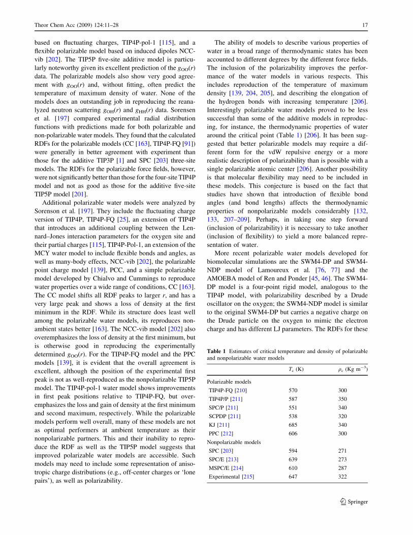
around the critical point (Table 1) [206]. It has been sug-

gested that better polarizable models may require a dif-ferent form for the vdW repulsive energy or a more

realistic description of polarizability than is possible with a

single polarizable atomic center [206]. Another possibilityis that molecular flexibility may need to be included in

these models. This conjecture is based on the fact that

studies have shown that introduction of flexible bondangles (and bond lengths) affects the thermodynamic

properties of nonpolarizable models considerably [132,

133, 207–209]. Perhaps, in taking one step forward(inclusion of polarizability) it is necessary to take another

(inclusion of flexibility) to yield a more balanced repre-

sentation of water.More recent polarizable water models developed for

biomolecular simulations are the SWM4-DP and SWM4-

NDP model of Lamoureux et al. [76, 77] and theAMOEBA model of Ren and Ponder [45, 46]. The SWM4-

DP model is a four-point rigid model, analogous to the

TIP4P model, with polarizability described by a Drudeoscillator on the oxygen; the SWM4-NDP model is similar

to the original SWM4-DP but carries a negative charge on

the Drude particle on the oxygen to mimic the electroncharge and has different LJ parameters. The RDFs for these

Table 1 Estimates of critical temperature and density of polarizableand nonpolarizable water models

Tc (K) qc (Kg m-3)

Polarizable models

TIP4P-FQ [210] 570 300

TIP4P/P [211] 587 350

SPC/P [211] 551 340

SCPDP [211] 538 320

KJ [211] 685 340

PPC [212] 606 300

Nonpolarizable models

SPC [203] 594 271

SPC/E [213] 639 273

MSPC/E [214] 610 287

Experimental [215] 647 322

Theor Chem Acc (2009) 124:11–28 17

123

models are characterized by the narrow shape of the first

peak in the gOO(r) radial distribution and the first intra-molecular peak of the gOH(r) distribution is slightly out-

ward (rOH(1) = 1.85 A instead of 1.78 A). The height of the

first peak in the oxygen–oxygen radial distribution functionis 3.07, which is somewhat high but almost within the

experimental error from the neutron diffraction results

(gOO(1) (r) = 2.7 ± 0.3 [216]). Notably, the SWM4 models

accurately reproduce the diffusion coefficient and are in

satisfactory agreement with experiment for the Debye andNMR relaxation times, indicating their accurate treatment

of dynamic properties. These models also accurately

reproduce the dielectric constant of water, e, which is notsurprising given that e was included as target data during

optimization of those models. Interestingly, that effort lead

to the observation that the gas phase polarizability of water,as well as other molecules, may not be appropriate for the

condensed phase. This is consistent with observations

based on quantum calculations, as discussed in detailbelow. While the question of polarizability scaling is still

being addressed (see below), it should be emphasized that a

proper treatment of the dielectric behavior of water as wellas other molecules is important for accurate treatment of

solvation energies in different environments and, accord-

ingly, its accurate reproduction by a model may be con-sidered an essential feature.

The AMOEBA water model of Ren and Ponder [45] is

fully flexible and was compared with experimental and QMdata. Studies of single isolated molecules, molecular clus-

ters, liquid water and ice were performed. AMOEBA cal-

culated dipole and quadrupole moments and polarizabilityof an isolated water molecule were shown to be in good

agreement with experimental and QM results. Tests of the

water dimer were also conducted and it was found to be ingood agreement with recent theoretical results [217, 218].

Bonding energies and geometries of small water clusters

from the trimer to the hexamer were also found to be ingood agreement with QM results [219, 220]. Simulations of

liquid water were performed and thermodynamic, transport

and structural results were compared with experimentaldata. Of the several quantities computed, density at room

temperature and heat of vaporization were in excellent

agreement with experimental values, the dielectric constantwas slightly higher than the experimental value, the self-

diffusion coefficient was lower than the experiment and the

viscosity was higher as expected. The structure of liquidwater was characterized by computation of OO, OHand HH RDFs sampled from NPT simulations and

compared with Soper’s 2000 results [190]. It is noteworthythat the experimental curves gOO reported by Soper in 2000

(neutron-diffraction) are almost identical to the ones of

Sorensen et al. (X-ray experiments) [197]. The position ofthe first peak in the gOO(r) radial distribution from the

AMOEBA simulations is 0.08 A longer and its height is

higher than that of the Soper 2000 RDF. The first peaks ofthe gOH(r) and gHH(r) RDFs are also higher that the Soper

2000 data and the positions of the two peaks are shifted to

larger distances. In general, the model provides a credibledescription of the structural properties of bulk liquid water

at room temperature. Studies of two ice forms, ice Ih and

XI, were also reported through energy minimization ofatomic positions and crystal lattices and MD simulations.

The computed results are in very good agreement with theexperimental data. The same authors published another

study where the temperature and pressure dependence of

the AMOEBA water model are analyzed [46].

3.2 Ion solvation

One of the most critical needs for a biological polarizable

force field is the treatment of both atomic and molecular

ions. Ion solvation is important in chemistry, includingsurface chemistry, environmental chemistry, and the study

of molecules such as surfactants, colloids, and polyelec-

trolytes. Biologically, ions are critical to the structure andfunction of nucleic acids, proteins, and lipid membranes

and ion transport in and out of the cell plays a central role

in numerous physiological processes [221–225]. Thestructure of nucleic acids is affected by nonspecific coun-

terion condensation [226] as well as specific interactions

[227, 228]. Ion binding to specific protein sites occurs forpurposes of stabilization as well as playing central roles in

enzyme catalysis [229–231]. Ion permeation across the cell

membrane is tightly controlled by specialized proteinscalled ion channels [232–234]. In physical chemistry, ion

solvation is also important in several processes such as

chemical purification [235] and chromatographic systems[236] and ion-specific chelators [237].

Simulations of aqueous ionic solutions using nonpolari-

zable additive force fields have shown that considerationof non-additive effects is important to accurately reproduce

the atomic details of ion hydration [43, 116, 150, 173, 238–

240]. In principle, accurate potential functions for com-puter simulations can be developed and validated by

comparing to experimental data (gas phase and bulk) and to

the results of high level QM ab initio computations per-formed on ion–water dimers and small ion-solvent clusters

[43, 79]. Experimental target data available to parametrize

and validate MM models of ion–water systems include gasphase energies of small hydrated clusters [241], bulk

hydration free energies [242, 243], structural properties

(radial distribution function, coordination numbers, etc.),and transport coefficients (diffusion constant, mobility,

conductivity). Aqvist was the first to develop additive ion–

water interaction potentials for the most common ions inbiology using calculations of the absolute hydration free

18 Theor Chem Acc (2009) 124:11–28

123

energy in bulk water [244]. The models were constructed

for the nonpolarizable SPC water model, but have alsobeen translated for the TIP3P and TIP4P model, giving rise

to a number of unanticipated issues (see recent article by

Cheatham [245]). A similar route was taken to develop anindependent set of ions for the TIP3P model [246, 247].

Correct interpretation of the experimental hydration free

energies of ions and its use in constructing an accuratecomputational model is, in fact, not as straightforward as

one would wish [78, 79]. One difficulty arises becauseexperimental thermodynamic or electrochemical measure-

ments involve neutral macroscopic systems and have

access only to irreducible, conventional hydration freeenergies that are either the sum of the absolute free ener-

gies of an ion and a counterion, DGhyd(M?) ? DGhyd(X

-),

or the difference of the free energies of two ionic species ofthe same valence, DGhyd(M1

?) ? DGhyd(M2?). In fact, the

absolute hydration free energy of a single ion cannot be

resolved from calorimetric or electrochemical experimentsalone. So, while the solvation free energy for a neutral salt

can be measured, it is impossible to separate it experi-

mentally into contributions from the cation and anion [242,248, 249]. An additional extrathermodynamic assumption

is required to perform this dissection [250]. A detailed

explanation of the pros and cons of the different methodscan be found in Ref. [43] and in [78]. In the same refer-

ences, alternative methods were proposed to deal with this

assumption. Lamoureux and Roux examined the sensitivityof the bulk hydration free energy of individual ions to the

gas phase monohydrate energy and showed that the abso-

lute scale varies only within a narrow range. The impli-cation is that the gas phase monohydrate energies puts, by

itself, a tight constraint on the absolute scale of hydration

free energies of ions. This analysis was used to set theabsolute scale of hydration free energy and develop a

consistent parametrization for the complete alkali-halide

series. This type of analysis, relating monohydrate and bulksolvation properties, goes back to the pioneering study of

Aqvist [244].

Several studies of the solvation of ions and salts havebeen published using the different polarizable models

implemented in CHARMM. Lamoureux and Roux deve-

loped polarizable potential functions for the hydration ofalkali and halide ions using the SWM4-DP water model.

Patel and co-workers published several studies of solvation

of ions and salts in water using the polarizable TIP4P-FQwater model implemented in CHARMM [251–253]. In

another study from that laboratory [251] the TIP4P-FQ

model was compared with the additive TIP4P and theDrude water models. Roux and co-workers have presented

a study of aqueous solvation of K? and compared ab initio,

polarizable (SWM4-NDP Drude water model ofCHARMM) and additive force field methods [79]. All

computational methods yielded hydration numbers

between 5.9 (Car-Parrinello PW91/pw) and 6.8 (Drudemodel) in good agreement with experimental data (6–7).

Other authors have presented studies relevant to under-

stand the performance of electronic polarization in inter-actions of molecules with ions. Masia and co-workers

[254] studied the interaction of a molecule with a cation,

via induced dipoles and Drude oscillators. The dimerelectric dipole moments as a function of the ion-molecule

distance for selected molecular orientations was comparedwith high-level ab initio calculations for water or carbon

tetrachloride close to Li?, Na?, Mg2?, and Ca2?. It was

shown that the simple polarization methods are able tosatisfactorily reproduce the induced dipole moment of the

cation-molecule dimer. In a previous study, the same

authors studied the interactions between molecules andpoint charges [255].

A potential model for Li?-water clusters was presented

[256] and the same authors performed a detailed study ofthe monovalent ions, Li?, Na?, K?, F-, Cl-, and Br- in

aqueous solution and the small water clusters M?(H2O)nand M-(H2O)n. These studies were based on the ABEEM/MM method. Analysis of results from these studies inclu-

ded solvation structures, charge distributions, binding

energies, dynamic properties (diffusion coefficients ofions) and free energies of hydration [257]. The computed

quantities were found to be in good agreement with

experimental results.A study of solvation dynamics of divalent cations in

water was performed by Piquemal et al. [258] using a

modified AMOEBA force field. The model consisted of acation specific parametrization based on ab initio polari-

zation energies computed by a constrained space orbital

variation (CSOV) energy decomposition method [259].Excellent agreement between computed and experimental

condensed phase properties was found despite the use of

parameters derived from gas phase ab initio calculations.A number of studies of the influence of ions on the air–

water interface using polarizable models have been pub-

lished. A useful review of these studies is that by Jungwirthand Tobias [260]. Examples include the study of Salvador

et al. of the aqueous solvation of NO3- in interfacial

environments with a Car-Parrinello MD simulation of acluster and classical MD of an extended slab system with

bulk interfaces using a polarizable force field based on the

atoms in molecules analysis (AIM) [261]. Both in aqueousclusters and in systems with extended interfaces the nitrate

anion clearly prefers interfacial over bulk solvation.

Archontis and co-workers studied the distribution of iodineat the air–water interface using the Drude based SWM4-DP

water model [262, 263] and Jungwirth and co-workers

performed similar studies using the AMOEBA force field[264]. In all cases it was found that iodine tends to remain

Theor Chem Acc (2009) 124:11–28 19

123

closer to the water/vapor and that tendency to stay at the

interface increases in the order Cl- \ Br- \ I-. Morerecently, studies of several ions and salts at the air–water

interface have been published. Tobias and co-workers have

presented a mixed X-ray photoemission spectroscopy/MDstudy using polarizable potentials of aqueous potassium

fluoride solutions [265]. Wang et al. studied NaCl using

a Drude model [266] and Warren and Patel comparedseveral polarizable ion models [252, 253]. MD studies of

aqueous solutions of molecular ions have also been pub-lished. Picalek et al. [267] studied the interfacial structure

of aqueous solutions of 1-butyl-3-methylimidazolium

tetrafluoroborate and 1-butyl-3-methylimidazolium hexa-fluorophosphate using both non-polarizable and polarizable

force fields.

Specialized uses of combined QM and MD methodshave been presented. Roos and co-workers [268] studied

the coordination environment of the uranyl ion in water.

Pair potentials were initially calculated using multiconfigu-rational wave function calculations and the quantum

chemically determined energies were used to fit parameters

in a polarizable force field with an additional chargetransfer term. Classical MD simulations were performed

for the uranyl ion and up to 400 water molecules. The

results show a uranyl ion with five water molecules coor-dinated in the equatorial plane. The U-O(H2O) distance is

2.40 A and a second coordination shell starts at about

4.7 A from the uranium atom. Interestingly, no hydrogenbonding is found between the uranyl oxygens and water.

In summary, polarizable force fields have been shown to

be very promising for simulating the properties of ionicsystems. Particularly satisfying, though not surprising, is

their ability to successfully describe interfacial systems

more accurately than additive models. This further empha-sizes the importance of the ability of polarizable models

to accurately treat environments of varying polarity to pro-

duce a more accurate representation of the experimentalregimen.

3.3 Application of polarizable models to smallmolecules

A number of small molecules have been studied usingpolarizable force fields. Examples include the major

organic functional groups, for example, pure alkanes,

alcohols, thiols, aromatic compounds, aldehydes, ketones,ethers, amines and amides; chlorinated compounds,

including CCl4 and CH2Cl2, and the guanidinium ion.

Many studies included the compounds in aqueous solution.Early studies of small organic molecules were limited to

determination of electrostatic properties using polarizable

methods. No et al. applied an electronegativity equalizationmethod to determine net atomic charges of 25 small

organic molecules including alcohols, ethers, esters, alde-

hydes, ketones, thiols, thioethers, secondary amines andalkanes [269], and to ionic and aromatic compounds [270].

An early condensed phase study of polarizable alkanes

was presented by Rick and Berne [184]. The manuscriptreported the free energy of methane association in water

using a polarizable fluctuating charge model. Two previous

studies only included polarizability on the water molecules[183, 271]. The hydrophobic interaction was more recently

analyzed using polarizable models by Rick [272], whocalculated the heat capacity change for methane pair

aggregation. Chelli and co-workers [126] applied the

fluctuating point charge model (FQ) and the atom–atomcharge transfer model (AACT), fitted to the polarizability

of small alkanes and polyenes, to larger homologues.

The AACT scheme was found to perform better on alkanesof any length and conformation. The AACT scheme also

satisfactorily reproduced the polarization response for

highly conjugated systems.A number of additional studies of alkanes using polari-

zable models have been reported. Bret et al. developedforce field parameters for methane in the framework of thechemical potential equalization model [97]. Studies of

methane clathrate hydrates were performed by English and

MacElroy [273] using flexible and rigid polarizable andnonpolarizable water and flexible and rigid methane mod-

els. Parametrization and testing of the ABEEM/MM fluc-

tuating charge force field for alkanes was described byZhang and Yang [274]. Borodin and Smith [275] reported

the development of many-body polarizable force fields

for ether, alkane and carbonate-based solvents. Alkaneparameters were also developed for the polarizable meth-

ods included in CHARMM. MacKerell and co-workers

presented a systematic study of a Drude oscillator-basedmodel of alkanes [85], calculating bulk thermodynamic,

structural, dielectric, and aqueous solvation properties.

Patel and Brooks [276] presented a study on a polarizablemodel of hexane in the framework of the fluctuating charge

method, focusing on bulk liquid phase properties and

analysis of the hexane–water interface. Recently, thiswork was extended to include longer alkanes by Davis

et al. [277]. Development of a polarizable intermolecular

potential function (PIPF) for liquid amides and alkaneshas been reported [36]. Another application reported by

Jalkanen and Zerbetto [278] studied the adsorption of

organics on a silver surface using an embedded atom modelfor the metal, a standard bonded potentials for the organics,

and a combination of the charge equilibration model and

the Morse potential for their electrostatic and nonbondinginteractions.

Alcohols were the subject of several studies using

polarizable force fields. One of the earliest studies of anonadditive MD simulation of a pure alcohol was reported

20 Theor Chem Acc (2009) 124:11–28

123

by Caldwell and Kollman, who studied the structure and

properties of pure methanol [279]. This was followed bycalculation of the aqueous solution free energy of methanol

[280]. Chelli and co-workers applied the chemical potential

equalization method to calculate the optical spectra ofliquid methanol [96, 98] and investigated the polarization

response of methanol by polarizable force field and density

functional theory calculations [281]. The method to modelpolarization developed by Ferenczy and Reynolds [282,

283] was also applied to methanol complexes [284].Methanol was also used in the development of the induced

dipole method of Berne, Friesner and co-workers [285]. A

polarizable model for simulation of liquid methanol wasdeveloped using the Charge-on-Spring (COS) technique

and is compatible with the COS/G2 water model. The

model was used to study the thermodynamic, dynamic,structural, and dielectric properties of liquid methanol and

of a methanol–water mixture [286]. MC simulations of

liquid methanol have also been reported using a potentialincluding polarizability, nonadditivity, and intramolecular

relaxation [287]. The classical Drude oscillator model

implemented in CHARMM was used to study water–eth-anol mixtures by Noskov et al. [68]. Interestingly, although

the water and ethanol models were parametrized separately

to reproduce their respective vaporization enthalpies, staticdielectric constants, and self-diffusion constants of the pure

liquids, the model was able to reproduce the energetic and

dynamical properties of the mixtures accurately. Further-more, the calculated dielectric constant for the various

water–alcohol mixtures is in excellent agreement with

experimental data. A revised Drude model for primary andsecondary alcohols has been presented by Anisimov et al.[69]. That work indicated significant differences in alco-

hol–water RDFs as compared to the CHARMM additiveforce field, suggesting that the inclusion of polarizability

alters atomic details of the interactions between these

classes of molecule. Parameters for ethanol and methanolhave also been developed for the FQ implementation in

CHARMM [288, 289]. Recently, thermodynamic and

structural properties of methanol–water solutions werepublished using that model [290]. Polarizable force fields

have also been developed for thiols and other sulfur

containing compounds like thioethers and disulfides.Noteworthy is the work of Kaminski et al. [285, 291] andsulfur parameters based on the Drude oscillator model are

in progress (X. Zhu and A.D. MacKerell, Jr., Work inprogress).

Other classes of small organic molecules studied with

polarizable force fields are aromatic and heteroaromaticcompounds. Stern et al. parameterized electrostatic

parameters of substituted benzenes based on fluctuating

charge, induced dipole, and a combined model and appliedthe resulting parameters to compute conformational

energies of the alanine, serine and phenylalanine dipeptides

[87]. The effort of Berne, Friesner and co-workers todevelop a polarizable force field for small organic mole-

cules within a fluctuating charge approach also included

benzene and phenol [291]. The development of the DRF90force field of Swart and van Duijnen relied on comparison

of computed interaction energies and geometries of ben-

zene dimers with ab initio results [29]. Lopes et al. pub-lished a study of aromatic compounds using the classical

Drude formalism implemented in CHARMM. Benzenedimer interaction energies and geometries were considered

and thermodynamic and transport properties in condensed

phase were computed and compared with experimentalvalues [70]. Soteras et al. developed models of distributed

atomic polarizabilities for the treatment of induction effects

in MM simulations within the framework of the induceddipole model. Molecular polarizabilities were computed for

benzene, pyridine, imidazole, indole, aniline, benzonitrile,

phenol and halogenated benzenes [292]. Mayer andAstrand developed a charge-dipole model for the static

polarizability of nanostructures that include aliphatic,

olephinic and aromatic systems [293]. MacKerell andco-workers have recently published force field parameters

for pyridine, pyrimidine, imidazole, pyrrole, indole and

purine [10], an effort that will lay the ground work for thedevelopment of a nucleic acids force field. That effort

relied heavily on the reproduction of a variety of experi-

mental condensed phase properties including pure solvents,crystals and aqueous solvation. Use of multiple types of

condensed phase data is important is it increases the

number of types of molecules that can be optimized usingexperimental thermodynamic data and the types of envi-

ronments that can be considered during the force field

optimization.Ethers, ketones and aldehydes are among the most

studied molecules using polarizable force field methods.

Shirts and Stolworthy [294] analysis of a crown ether (18-crown-6) showed that the electrostatic term is the largest

contributor to the conformational energy and discussed the

desirability of using a polarizable method, such as thecharge equilibration algorithms, to include these effects in

MM and MD calculations. During development of the FQ

method by Berne and co-workers investigations of theaqueous solvation and reoganization energy of other mol-

ecules, notably formaldehyde, were performed [295, 296].

The development of new schemes of including polarizationin classical force fields often used water-formaldehyde

complexes as a source of target data for the parametriza-

tion. The methods to model polarization developed byFerenczy and Reynolds [282, 283] and Krimm and

co-workers included formaldehyde–water complexes [284,

297]. Borodin and Smith developed classical polarizableforce fields for several molecules including polyethers,

Theor Chem Acc (2009) 124:11–28 21

123

ketones, and linear and cyclic carbonates on the basis of

QM dimer energies of model compounds and empiricalthermodynamic liquid-state properties [275, 298–304].

The first studies of amines and amides using polarizable

forcefieldswere the hydration calculationsbyKroghjespersenet al. [305], and of amine hydration by Kollman and

co-workers [306]. Despite the very different parametriza-

tions, inclusion of polarizability substantially improved thereproduction of the experimental free energies of aqueous

solvation in both studies. Amides, in particular N-methy-lacetamide (NMA), are extremely important in the devel-

opment of polarizable force fields for proteins since they

constitute the smallest unit representative of the polypep-tide backbone. Recently, MacKerell, Roux and co-workers

parametrization of NMA within the context of the classical

Drude polarizable method was the first force field toreproduce the large dielectric constant of liquid NMA [84].

Polarizable models of amide compounds that have two

(acetamide) and zero (N,N-dimethyl acetamide) polarhydrogen-bond donor atoms were also investigated. In

those studies it was shown that a proper representation of

both the magnitude and direction of the molecular polari-zability tensor, made possible by the use of atom-based

Thole damping factors, was essential to obtain the correct

dielectric response.The ability of polarizable force fields to accurately

reproduce dielectric constants deserves additional discus-

sion. Although the dielectric is a macroscopic property ofbulk system, it has a critical impact on microscopic inter-

actions within the system. This can be qualitatively illus-

trated by considering the familiar Born model of solvation,which shows that the solvation free energy of an ion of

charge q and radius R is given by q2/(2R) (1/e - 1). This

expression shows that correct estimation of e is essential toobtain the proper solvation thermodynamics. The treatment

of induced electronic polarization becomes of particular

importance in the case of the low-dielectric alkanes. Thecorrect value of e is approximately 2, which is only pos-

sible to attain in polarizable models as additive models

with fixed partial charges yield values that are approxi-mately equal to 1 [85]. Obviously, going from a value of

1 to 2 drastically impacts solvation energies, as shown in

the context of the Born approximation, such that the abilityof force fields to model relative solvation in complex

simulations, such as lipid bilayers, will be drastically

effected. For example, the neglect of polarization of thehydrocarbon core of lipid membranes has been shown to

have great practical consequences in computational studies

of ion channels [307, 308]. However, attaining the correctdielectric behavior appears to not be trivial. In our own

hands, the assumption that the gas phase polarizabilities

would be applicable to the condensed phase was shownto be incorrect on the first molecule studied, water, as

discussed above. This lead to the development of an

approach whereby the polarizability of a molecule is con-sidered a free parameter during optimization, with the

primary target data being reproduction of the dielectric

constant of the corresponding pure solvent. To date, ourefforts indicate that the appropriate polarizability depends

on the class of molecule under study. As quantified in terms

of scaling of the gas phase polarizability, we have empiri-cally determined scaling factors ranging from 0.7 for

water, alcohols and sulfur containing species, 0.85 for aro-matics, N-containing heteroaromatics and ethers (C. Baker

and A.D. MacKerell, Jr. Work in progress) and 1.0 for

amides. Given the role of electrostatics in a variety ofcomplex phenomena involving biological systems (e.g.,

pKas, reduction potentials) and the contribution of the

dielectric to proper treatment of electrostatics, carefulconsideration of this important term is central to successful

development of polarizable force fields for biological

molecules.QM studies also indicate that polarizability scaling for

the condensed phase may be necessary. Based on studies of

water clusters, it was suggested that in the condensedphase, polarization is lower than in gas phase because of

the energetic cost arising from Pauli’s exclusion principle

due to the overlap of neighbouring electronic charge dis-tributions [309]. A recent study by Schropp and Tavan

[310] on the polarization of a single QM water molecule

within a MM described bulk phase also concluded that thegas phase experimental polarizability cannot be used in

molecular simulations but must be reduced to an effective

polarizability. It was argued that in the liquid phase theelectric field, Eh i, in the excluded volume of each water

molecule is strongly inhomogeneous such that the electric

field at the position of the oxygen (or hydrogens), E(rO), isnot appropriate for calculation of the molecular polari-

zability. Since Eh i is smaller than E(rO) and it is necessary

to use E(rO) in MD simulations because of computationalefficiency, results that E(rO) needs to be scaled to match

Eh i. Remarkably, the scaling factor proposed by Schropp

and Tavan (0.68) is close to the empirical value ofapproximately 0.7 proposed by Lamoureux et al. [76, 77].

Another recent study using semiempirical methods on

model compounds representative of phospholipids alsoindicated that the polarizability of the head group

decreased in the presence of water, suggesting the effect is

due to making ‘‘electrons in hydrogen bonds to be morebound’’ [311]. However, the AMEOBA water model,

which has been developed with inducible point-dipoles on

the oxygen as well as on the hydrogen atoms without anyscaling, only slightly overestimates the dielectric of bulk

water under ambient conditions (see above), indicating that

the extent of scaling may also be dependent on the methodused to treat polarizability. Thus, while both QM as well as

22 Theor Chem Acc (2009) 124:11–28

123

empirical approaches based on reproduction of condensed

phase properties indicate the need for polarizability scalingfor some classes of molecules, the cause of the effect is still

a matter of debate.

In general, the simulation studies of small moleculesusing polarizable models have shown that the extension of

empirical force fields to include polarization is indeed fea-

sible. In many, but not all cases the polarizable models havelead to improved agreement with experiment. In addition,

the atomic details of the interactions between components incondensed phase simulations have been observed to differ in

polarizable models as compared to additive models [70, 85].

Thus, it appears that polarizable models will lead to a moreaccurate picture of the atomic details of condensed phases;

however, it should emphasized that careful optimization

methods, including optimization of the LJ parameters,followed by rigorous validation of the models is essential

to assure that those models are yielding atomic pictures

representative of the experimental regimen.

3.4 Application of polarizable force fields to proteins,

nucleic acids and lipid bilayers

The ultimate goal of polarizable force fields with biological

relevance is the development of fully usable, high qualityforce fields applicable to simulations of large biomole-

cules: proteins, DNA/RNA, lipid bilayers and carbohy-

drates. While the development of such force fields thathave been fully optimized is still in its infancy, very early

studies that applied polarizable models to proteins in MM

calculations should be noted. These include a study oflysozyme by Warshel and Levitt [312] who simulated

the electrostatic environment by a polarizable force field

based on induced dipoles and represented the effect of thesurrounding solvent by a microscopic dielectric model.

Similar approaches were used for other systems [138, 313,

314]. While these studies only involved single point cal-culations (i.e. calculation of the polarization response on a

single protein conformation), they emphasize that early

workers were well aware of the importance of this term intheoretical studies of macromolecules. And given that it

has taken over 25 years since those seminal works to start

to systematically apply polarizable models to macromole-cules, it is clear that the technical hurdles to the imple-

mentation and development of polarizable models have and

will continue to be large. Only recently has there was asurge of publications on large molecules indicating that

many of the polarizable force fields being developed in the

past 10 years are nearing completion [315]. At the time ofwriting, many studies are still focused on validating the

various force fields that have been developed over the

years. However, fully featured studies that address specificresearch have already been published.

One of the first modern applications of a polarizable

force field to a protein was on crambin using the fluctuatingcharge method interfaced with the UFF and AMBER force

fields [111]. The polarizable charges were found to give

more realistic charge redistribution between amino acids inthe protein. Berne and co-workers used a combination of

permanent and inducible point dipoles with fluctuating

and fixed charges to simulate bovine pancreatic trypsininhibitor (BPTI) in water with two commonly used water

models TlP4P-FQ and RPOL. The simulated structuresremain within 1 A of the experimental crystal structure for

the 2 ns duration of the simulations [316, 317]. The extent

of deviation of the structure was similar to that obtain withthe OPLS all-atom additive force field. More recently,

Liang and Walsh studied aqueous solvation of carboxylate

groups present in the glycine zwitterion and the dipeptideaspartylalanine using the AMOEBA force field. Results

were compared with Car-Parrinello MD data and additive

force fields. The polarizable force field yields carboxylatesolvation properties in very good agreement with CPMD

results, agreement that was significantly closer than that

obtained from traditional force fields [318].Llinas et al. performed structural studies of human

alkaline phosphatase using the TCPEp (topological and

classical polarization effects for proteins) force field [319].The enzyme possesses 4 metal binding sites, two for Zn2?,

one for Mg2? and one Ca2?. In this study, Ca2? was

replaced by Sr2?, both showing similar interaction energiesat the calcium-binding site. Only at high doses of stron-

tium, comparable to those found for calcium, can strontium

substitute for calcium. Since osteomalacia is observed afteringestion of high doses of strontium, alkaline phosphatase

is likely to be one of the targets of strontium, and thus the

results support the suggestion that the enzyme may beinvolved in this disease.

In a step forward towards a polarizable force field for

proteins Wang et al. optimized the the AMBER polarizablemodel parameters adjusting the phi and psi torsion angles

of the protein backbone by fitting to the QM energies of

the important regions: beta, P-II, alpha(R), and alpha(L)regions [320]. Performance of the force field was analysed

by comparison of energies against QM data and by the

replica exchange molecular dynamics simulations of shortpolyalanine peptides in water. The populations in these

three regions were found to be in qualitative agreement

with the NMR and CD experimental results.The ABEEM/MM method has been tested in studies of

peptides and proteins. The first of those studies is a con-

formational analysis of a peptide in 2006 [321], followedby studies of trypsin inhibitors [322], BPTI in aqueous

solution and conformational studies of alpha-conotoxin GI

[323]. A study on the geometry of the heme prostheticgroup was also published in 2008 [324].

Theor Chem Acc (2009) 124:11–28 23

123

Extension of polarizable force fields to studies of other

classes of biomolecules has also been published. Allen andco-workers compared newly developed coarse-grained

models, with the additive CHARMM27 force field and the

newly developed Drude force field on the energetics ofmembrane–arginine interactions [325]. An innovative

application of polarizable force fields was presented by

Masella and co-workers, who combined a polarizable forcefield and a coarse-grained polarizable solvent with appli-

cation to a long simulation of bovine pancreatic trypsininhibitor [326]. The method was found to be much faster

than traditional approaches where solvent is treated atom-

istically. Specialized applications included application of apolarizable force field to calculation of protein-ligand

binding energies [327] and calculation of the infrared

spectra of the polypeptide backbone [328].The first application of polarizability to an MD simu-

lation of DNA using the Drude oscillator model was per-

formed by MacKerell and co-workers [82] in combinationwith the CHARMM27 all-atom nucleic acid force field

[34]. The system included a DNA octamer and a full sol-

vent representation based on the SWM4-DP model withsodium counterions. The simulation system was shown to

be stable, ultimately for 5 ns, though the RMS difference

with respect to canonical B form DNA continuallyincreased, well beyond that of a simulation using the

CHARMM27 additive model. This deviation emphasizes

the importance of full optimization of a force field whenthe electrostatic model is changed. This is due to the

electronic term affecting geometries, vibrations and con-

formational energies as well as interactions with the envi-ronment. More recently, Sagui and co-workers performed

molecular dynamics simulations of a DNA decamer using

both additive atomic point charge and polarizable forcefields [329–331]. Results showed the polarizable model

to yield properties similar to that of the additive FF,

which may be associated with the underpolarization of theinduced dipole model used in that study.

An updated overview of current DNA modeling with

ab initio (Hartree-Fock, density functional theory, and tightbinding approximations) and empirical methods including

polarizable methods has been published by Cozmuta and

Mehrez [332]. The authors extensively review the literatureuntil 2007. Another interesting review worth mentioning

discusses the merits and limitations of modeling methods

available for guanine quadruplex (G-DNA) molecules[333, 334]. Although not focused on polarizable force

fields it is an important source of information for the

computational chemist/biologist working in the field. Thereview discusses the relation of simulation results to

experimental techniques and the significance of those

relationships. Aspects such as: pair-additive approximationof the empirical force fields, sampling limitations due to

limited simulation times, accuracy of description of base

stacking, H-bonding, sugar-phosphate backbone and ionsby force fields, are addressed.

4 Summary

Empirical force fields that explicitly treat electronicpolarizability have been known for over 30 years. How-

ever, due to technical challenges associated with theirimplementation, difficulties in the optimization of suffi-

ciently accurate models, and computational demands it is

only in recent years that they have started to be increas-ingly considered. Over the last 15 years a large number of

studies using polarizable models of water, ions and of small

molecules have been published. The most notable insightsfrom these efforts are in the area of ion solvation and at

interfaces and it is evident that atomistic details of inter-

molecular interactions differ between polarizable andadditive force fields. With respect to macromolecules, a

number of works have been published over the last several

years with emphasis on the capabilities and accuracy ofpolarizable models, particularly of proteins. While the

application of polarizable models to macromolecular sys-

tems has been slow to get out of the gate, it is clear thatover the next decade highly optimized polarizable force

fields for these systems will become available and widely

used. We eagerly look forward to the novel insights thatwill be obtained from these studies.

Acknowledgments Financial support from the NIH (GM 51501 toA.D.M. and GM 072558 to B.R. and A.D.M.) is acknowledged.

References

1. Jorgensen WL, Chandrasekhar J, Madura JD et al (1983) J ChemPhys 79:926

2. Cornell WD, Cieplak P, Bayly CI et al (1995) J Am Chem Soc117:5179

3. MacKerell AD, Bashford D, Bellott M et al (1998) J Phys ChemB 102:3586

4. MacKerell AD Jr, Brooks B, Brooks CLIII et al (1998) In:Schleyer PVR et al (eds) Encyclopedia of computationalchemistry. John Wiley & Sons, Chichester

5. Scott WRP, Hunenberger PH, Tironi IG et al (1999) J PhysChem A 103:3596

6. Jorgensen WL, Tiradorives J (1988) J Am Chem Soc 110:16577. Halgren TA, Damm W (2001) Curr Opin Struct Biol 11:2368. Rick SW, Stuart SJ (2002) In: Lipkowitz KB, Boyd DB (eds)

Reviews in computational chemistry. Wiley-VCH, Hoboken, NJ9. Warshel A, Kato M, Pisliakov AV (2007) J Chem Theor

Comput 3:203410. Lopes PEM, Lamoureux G, MacKerell AD (2009) J Comp

Chem 30:182111. Bayly CI, Cieplak P, Cornell WD et al (1993) J Phys Chem

97:1026912. Mackerell AD (2004) J Comp Chem 25:1584

24 Theor Chem Acc (2009) 124:11–28

123

13. Dyke TR, Muenter JS (1973) J Chem Phys 59:312514. Gregory JK, Clary DC, Liu K et al (1997) Science 275:81415. Sprik M (1991) J Phys Chem 95:228316. Wallqvist A, Mountain R (1999) In: Lipkowitz KB, Boyd DB

(eds) Reviews in computational chemistry. Wiley-VCH, NewYork

17. Soetens JC, Costa M, Millot C (1998) Mol Phys 94:57718. Silvestrelli PL, Parrinello M (1999) J Chem Phys 111:357219. Silvestrelli PL, Parrinello M (1999) Phys Rev Lett 82:330820. Silvestrelli PL, Parrinello M (1999) Phys Rev Lett 82:541521. Badyal YS, Saboungi ML, Price DL et al (2000) J Chem Phys

112:920622. Gubskaya AV, Kusalik PG (2002) J Chem Phys 117:529023. Kuo IF, Tobias DJ (2001) J Phys Chem B 105:582724. Jorgensen WL (2007) J Chem Theory Comp 3:187725. Liu YP, Kim K, Berne BJ et al (1998) J Chem Phys 108:473926. Maple JR, Cao YX, Damm WG et al (2005) J Chem Theor

Comput 1:69427. Patel S, Brooks CL (2004) J Comp Chem 25:128. Patel S, Mackerell AD, Brooks CL (2004) J Comp Chem

25:150429. Swart M, van Duijnen PT (2006) Mol Simul 32:47130. Ma BY, Lii JH, Allinger NL (2000) J Comp Chem 21:81331. Thole BT (1981) Chem Phys 59:34132. Applequist J, Carl JR, Fung K-K (1972) J Am Chem Soc

94:295233. Kuyper LF, Hunter RN, Ashton D et al (1991) J Phys Chem

95:666134. Foloppe N, MacKerell AD (2000) J Comp Chem 21:8635. Stern HA, Rittner F, Berne BJ et al (2001) J Chem Phys

115:223736. Xie WS, Pu JZ, MacKerell AD, Gao J (2007) J Chem Theor

Comput 3:187837. Gao JL, Habibollazadeh D, Shao L (1995) J Phys Chem

99:1646038. Gao JL, Pavelites JJ, Habibollazadeh D (1996) J Phys Chem

100:268939. van Duijnen PT, Swart M (1998) J Phys Chem A 102:239940. Xie W, Pu J, Gao J (2009) J Phys Chem A 113:210941. Ferenczy GG, Reynolds CA (2001) J Phys Chem A 105:1147042. Ren PY, Ponder JW (2002) J Comp Chem 23:149743. Grossfield A, Ren PY, Ponder JW (2003) J Am Chem Soc

125:1567144. Grossfield A, Ren PY, Ponder JW (2003) Biophys J 84:94A45. Ren PY, Ponder JW (2003) J Phys Chem B 107:593346. Ren PY, Ponder JW (2004) J Phys Chem B 108:1342747. Grossfield A (2005) J Chem Phys 122:02450648. Jiao D, King C, Grossfield A et al (2006) J Phys Chem B

110:1855349. Rasmussen TD, Ren PY, Ponder JW et al (2007) Int J Quantum

Chem 107:139050. Drude P (1902) The theory of optics. Kessinger Publishing

Company, MT (2008)51. London F (1937) Trans Faraday Soc 33:8b52. Bade WL (1957) J Chem Phys 27:128053. Bade WL, Kirkwood JG (1957) J Chem Phys 27:128454. Bade WL (1958) J Chem Phys 28:28255. Whitfield TW, Martyna GJ (2006) Chem Phys Lett 424:40956. Amos AT (1996) Int J Quantum Chem 60:6757. Wang F, Jordan KD (2002) J Chem Phys 116:697358. Dick BG, Overhauser AW (1958) Phys Rev 112:9059. Hanlon JE, Lawson AW (1959) Phys Rev 113:47260. Jacucci G, McDonald IR, Singer K (1974) Phys Lett A 50:14161. Lindan PJD, Gillan MJ (1993) J Phys: Condens Matter 5:101962. Mitchell PJ, Fincham D (1993) J Phys: Condens Matter 5:103163. Lindan PJD (1995) Mol Simul 14:303

64. Hoye JS, Stell G (1980) J Chem Phys 73:46165. Pratt LR (1980) Mol Phys 40:34766. Lado F (1997) J Chem Phys 106:470767. Cao J, Berne BJ (1993) J Chem Phys 99:221368. Noskov SY, Lamoureux G, Roux B (2005) J Phys Chem B

109:670569. Anisimov VM, Vorobyov IV, Roux B et al (2007) J Chem Theor

Comput 3:192770. Lopes PEM, Lamoureux G, Roux B et al (2007) J Phys Chem B

111:287371. Saint-Martin H, Medina-Llanos C, Ortega-Blake I (1990)

J Chem Phys 93:644872. de Leeuw NH, Parker SC (1998) Phys Rev B 58:1390173. Saint-Martin H, Hernandez-Cobos J, Bernal-Uruchurtu MI et al

(2000) J Chem Phys 113:1089974. van Maaren PJ, van der Spoel D (2001) J Phys Chem B

105:261875. Yu HB, Hansson T, van Gunsteren WF (2003) J Chem Phys

118:22176. Lamoureux G, MacKerell AD, Roux B (2003) J Chem Phys

119:518577. Lamoureux G, Harder E, Vorobyov IV et al (2006) Chem Phys

Lett 418:24578. Lamoureux G, Roux B (2006) J Phys Chem B 110:330879. Whitfield TW, Varma S, Harder E et al (2007) J Chem Theor

Comput 3:206880. Lu ZY, Zhang YK (2008) J Chem Theor Comput 4:123781. Lamoureux G, Roux B (2003) J Chem Phys 119:302582. Anisimov VM, Lamoureux G, Vorobyov IV et al (2005) J Chem

Theor Comput 1:15383. Harder E, Anisimov VM, Vorobyov IV et al (2006) J Chem

Theor Comput 2:158784. Harder E, Anisimov VM, Whitfield TW et al (2008) J Phys

Chem B 112:350985. Vorobyov IV, Anisimov VM, MacKerell AD (2005) J Phys

Chem B 109:1898886. Vorobyov I, Anisimov VM, Greene S et al (2007) J Chem Theor

Comput 3:112087. Stern HA, Kaminski GA, Banks JL et al (1999) J Phys Chem B

103:473088. Banks JL, Kaminski GA, Zhou RH et al (1999) J Chem Phys

110:74189. Kaminski GA, Stern HA, Berne BJ et al (2002) J Comp Chem

23:151590. Yin DX, Mackerell AD (1998) J Comp Chem 19:33491. Rick SW, Stuart SJ, Berne BJ (1994) J Chem Phys 101:614192. Nalewajski RF (1991) Int J Quantum Chem 40:26593. Chelli R, Procacci P (2002) J Chem Phys 117:917594. Itskowitz P, Berkowitz ML (1997) J Phys Chem A 101:568795. Nalewajski RF (1998) Pol J Chem 72:176396. Chelli R, Ciabatti S, Cardini G et al (1999) J Chem Phys

111:421897. Bret C, Field MJ, Hemmingsen L (2000) Mol Phys 98:75198. Chelli R, Ciabatti S, Cardini G et al (2000) J Chem Phys

112:551599. Nalewajski RF (2000) Int J Quantum Chem 78:168100. Llanta E, Ando K, Rey R (2001) J Phys Chem B 105:7783101. York DM, Yang WT (1996) J Chem Phys 104:159102. Smith PE (2004) J Phys Chem B 108:16271103. Chelli R, Barducci A, Bellucci L et al (2005) J Chem Phys

123:194109104. Medeiros M (2005) Theor Chem Acc 113:178105. Piquemal JP, Chelli R, Procacci P et al (2007) J Phys Chem A

111:8170106. Warren GL, Davis JE, Patel S (2008) J Chem Phys 128:144110107. Zhang Y, Lin H (2008) J Chem Theor Comput 4:414

Theor Chem Acc (2009) 124:11–28 25

123

108. Rappe AK, Goddard WA (1991) J Phys Chem 95:3358109. Kitao O, Ogawa T (2003) Mol Phys 101:3110. Nistor RA, Polihronov JG, Muser MH et al (2006) J Chem Phys

125:094108111. Ogawa T, Kurita N, Sekino H et al (2004) Chem Phys Lett

397:382112. Sefcik J, Demiralp E, Cagin T et al (2002) J Comp Chem

23:1507113. Tanaka M, Siehl HU (2008) Chem Phys Lett 457:263114. Brodersen S, Wilke S, Leusen FJJ et al (2005) Cryst Growth Des

5:925115. Chen B, Xing JH, Siepmann JI (2000) J Phys Chem B 104:2391116. Stuart SJ, Berne BJ (1996) J Phys Chem 100:11934117. Stuart SJ, Berne BJ (1999) J Phys Chem A 103:10300118. Rick SW, Berne BJ (1996) J Am Chem Soc 118:672119. Toufar H, Baekelandt BG, Janssens GOA et al (1995) J Phys

Chem 99:13876120. Parr RG, Pearson RG (1983) J Am Chem Soc 105:7512121. Kitaura K, Morokuma K (1976) Int J Quantum Chem 10:325122. Weinhold F (1997) J Mol Struct Theochem 398–399:181123. van der Vaart A, Merz KM (1999) J Am Chem Soc 121:9182124. Korchowiec J, Uchimaru T (2000) J Chem Phys 112:1623125. Jeziorski B, Moszynski R, Szalewicz K (1994) Chem Rev

94:1887126. Chelli R, Procacci P, Righini R et al (1999) J Chem Phys

111:8569127. Yang ZZ, Wang CS (1997) J Phys Chem A 101:6315128. Wang CS, Li SM, Yang ZZ (1998) J Mol Struct Theochem

430:191129. Wang CS, Yang ZZ (1999) J Chem Phys 110:6189130. Cong Y, Yang ZZ (2000) Chem Phys Lett 316:324131. Yang ZZ, Wang CS (2003) J Theor Comput Chem 2:273132. Yang ZZ, Wu Y, Zhao DX (2004) J Chem Phys 120:2541133. Wu Y, Yang ZZ (2004) J Phys Chem A 108:7563134. Parr RG, Yang W (1989) Density-Functional Theory of Atoms

and Molecules. Oxford University Press, Oxford135. Field MJ (1997) Mol Phys 91:835136. Gao JL (1997) J Phys Chem B 101:657137. Gao JL (1998) J Chem Phys 109:2346138. van Belle D, Couplet I, Prevost M et al (1987) J Mol Biol

198:721139. Svishchev IM, Kusalik PG, Wang J et al (1996) J Chem Phys

105:4742140. Bernardo DN, Ding YB, Kroghjespersen K et al (1994) J Phys

Chem 98:4180141. Medeiros M, Costas ME (1997) J Chem Phys 107:2012142. Campbell T, Kalia RK, Nakano A et al (1999) Phys Rev Lett

82:4866143. Car R, Parrinello M (1985) Phys Rev Lett 55:2471144. van Belle D, Wodak SJ (1995) Comput Phys Comm 91:253145. Tuckerman ME, Martyna GJ (2000) J Phys Chem B 104:159146. Tuckerman ME, Martyna GJ (2001) J Phys Chem B 105:

7598147. van Belle D, Froeyen M, Lippens G et al (1992) Mol Phys

77:239148. Sprik M, Klein ML (1988) J Chem Phys 89:7556149. Stillinger FH, David CW (1978) J Chem Phys 69:1473150. Lybrand TP, Kollman PA (1985) J Chem Phys 83:2923151. Barnes P, Finney JL, Nicholas JD et al (1979) Nature 282:459152. Rullmann JAC, van Duijnen PT (1988) Mol Phys 63:451153. Ahlstrom P, Wallqvist A, Engstrom S et al (1989) Mol Phys

68:563154. Cieplak P, Kollman P, Lybrand T (1990) J Chem Phys 92:6755155. Niesar U, Corongiu G, Clementi E et al (1990) J Phys Chem

94:7949156. Kuwajima S, Warshel A (1990) J Phys Chem 94:460

157. Caldwell J, Dang LX, Kollman PA (1990) J Am Chem Soc112:9144

158. Dang LX (1992) J Chem Phys 97:2659159. Kozack RE, Jordan PC (1992) J Chem Phys 96:3120160. Wallqvist A, Berne BJ (1993) J Phys Chem 97:13841161. Brodholt J, Sampoli M, Vallauri R (1995) Mol Phys 85:81162. Brodholt J, Sampoli M, Vallauri R (1995) Mol Phys 86:149163. Chialvo AA, Cummings PT (1996) J Chem Phys 105:8274164. Dang LX, Chang TM (1997) J Chem Phys 106:8149165. Wallqvist A, Ahlstrom P, Karlstrom G (1990) J Phys Chem

94:1649166. Halley JW, Rustad JR, Rahman A (1993) J Chem Phys 98:4110167. Corongiu G (1992) Int J Quantum Chem 42:1209168. Zhu SB, Singh S, Robinson GW (1991) J Chem Phys 95:2791169. Zhu SB, Yao S, Zhu JB et al (1991) J Phys Chem 95:6211170. Feyereisen MW, Feller D, Dixon DA (1996) J Phys Chem

100:2993171. Burnham CJ, Li JC, Xantheas SS et al (1999) J Chem Phys

110:4566172. Dang LX, Smith DE (1993) J Chem Phys 99:6950173. Sprik M, Klein ML, Watanabe K (1990) J Phys Chem 94:6483174. Xantheas SS, Dang LX (1996) J Phys Chem 100:3989175. Bryce RA, Buesnel R, Hillier IH et al (1997) Chem Phys Lett

279:367176. Cabarcos OM, Weinheimer CJ, Lisy JM (1999) J Chem Phys

110:8429177. Baik J, Kim J, Majumdar D et al (1999) J Chem Phys 110:9116178. Robertson WH, Diken EG, Price EA et al (2003) Science

299:1367179. Lightstone FC, Schwegler E, Hood RQ et al (2001) Chem Phys

Lett 343:549180. Bako I, Hutter J, Palinkas G (2002) J Chem Phys 117:9838181. Wallqvist A (1990) Chem Phys Lett 165:437182. Motakabbir KA, Berkowitz ML (1991) Chem Phys Lett 176:61183. New MH, Berne BJ (1995) J Am Chem Soc 117:7172184. Rick SW, Berne BJ (1997) J Phys Chem B 101:10488185. Soper AK, Phillips MG (1986) Chem Phys 107:47186. Dore JC (1991) J Mol Struct 250:193187. Dore JC, Blakey DM (1995) J Mol Liq 65–66:85188. Soper AK (1997) J Phys: Condens Matter 9:2717189. Jedlovszky P, Brodholt JP, Bruni F et al (1998) J Chem Phys

108:8528190. Soper AK (2000) Chem Phys 258:121191. Nakahara M, Matubayasi N, Wakai C et al (2001) J Mol Liq

90:75192. Narten AH, Levy HA (1972) In: Franks F (ed) Water a com-

prehensive treatise. Plenum Press, New York193. Page DI (1972) In: Franks F (ed) Water a comprehensive trea-

tise. Plenum Press, New York194. Narten AH, Thiessen WE, Blum L (1982) Science 217:1033195. Yamanaka K, Yamaguchi T, Wakita H (1994) J Chem Phys

101:9830196. Hura G, Sorenson JM, Glaeser RM et al (2000) J Chem Phys

113:9140197. Sorenson JM, Hura G, Glaeser RM et al (2000) J Chem Phys

113:9149198. Head-Gordon T, Hura G (2002) Chem Rev 102:2651199. Soper AK, Turner J (1993) Int J Mod Phys B 7:3049200. Soper AK, Bruni F, Ricci MA (1997) J Chem Phys 106:247201. Mahoney MW, Jorgensen WL (2000) J Chem Phys 112:8910202. Corongiu G, Clementi E (1992) J Chem Phys 97:2030203. Berendsen H, Postma JPM, van Gusteren WF (1981) In:

Pullman B et al (eds) Intermolecular forces. Reidel PublishingCompany, Dordrecht, The Netherlands

204. Jedlovszky P, Vallauri R (1999) Mol Phys 97:1157205. Rick SW (2001) J Chem Phys 114:2276

26 Theor Chem Acc (2009) 124:11–28

123

206. Jedlovszky P, Richardi J (1999) J Chem Phys 110:8019207. Mahoney MW, Jorgensen WL (2001) J Chem Phys 115:10758208. Saint-Martin H, Hernandez-Cobos J, Ortega-Blake I (2005)

J Chem Phys 122:224509209. Lopez-Lemus J, Chapela GA, Alejandre J (2008) J Chem Phys

128:174703210. Yezdimer EM, Cummings PT (1999) Mol Phys 97:993211. Kiyohara K, Gubbins KE, Panagiotopoulos AZ (1998) Mol Phys

94:803212. Svishchev IM, Hayward TM (1999) J Chem Phys 111:9034213. Berendsen HJC, Grigera JR, Straatsma TP (1987) J Phys Chem

91:6269214. Panagiotopoulos AZ (1987) Mol Phys 61:813215. Hill PG (1990) J Phys Chem Ref Data 19:1233216. Markovich G, Perera L, Berkowitz ML et al (1996) J Chem Phys

105:2675217. Klopper W, van Duijneveldt-van de Rijdt J, van Duijneveldt FB

(2000) Phys Chem Chem Phys 2:2227218. Tschumper GS, Leininger ML, Hoffman BC et al (2002) J Chem

Phys 116:690219. Lee HM, Suh SB, Lee JY et al (2000) J Chem Phys 112:9759220. Xantheas SS, Burnham CJ, Harrison RJ (2002) J Chem Phys

116:1493221. Kaplan JH (2002) Annu Rev Biochem 71:511222. Zhang CX, Lippard SJ (2003) Curr Opin Chem Biol 7:481223. Aleman EA, Lamichhane R, Rueda D (2008) Curr Opin Chem

Biol 12:647224. Al-Hashimi HM, Walter NG (2008) Curr Opin Struct Biol

18:321225. Chen PR, He C (2008) Curr Opin Chem Biol 12:214226. Manning GS (1978) Quart Rev Biophys 11:179227. Scott WG (1999) Curr Opin Chem Biol 3:705228. Draper DE (2004) Rna-a publication of the Rna society 10:335229. Bartlett GJ, Borkakoti N, Thornton JM (2003) J Mol Biol

331:829230. Harris ME, Christian EL (2003) Curr Opin Struct Biol 13:325231. Sigel RKO, Pyle AM (2007) Chem Rev 107:97232. Doyle DA, Cabral JM, Pfuetzner RA et al (1998) Science 280:69233. Dutzler R, Campbell EB, Cadene M et al (2002) Nature 415:287234. Jiang YX, Lee A, Chen JY et al (2003) Nature 423:33235. Okada T (1991) J Chem Soc Faraday Trans 87:3027236. Okada T (1998) Anal Sci 14:469237. Takeda Y, Kanazawa M, Katsuta S (2000) Anal Sci 16:929238. Dang LX, Rice JE, Caldwell J et al (1991) J Am Chem Soc

113:2481239. Roux B (1993) Chem Phys Lett 212:231240. Roux B, Karplus M (1995) J Comp Chem 16:690241. Dzidic I, Kebarle P (1970) J Phys Chem 74:1466242. Marcus Y (1986) J Chem Soc Faraday Trans I 83:233243. Tissandier MD, Cowen KA, Feng WY et al (1998) J Phys Chem

A 102:7787244. Aqvist J (1990) J Phys Chem 94:8021245. Cheatham TEIII (2005) In: Spellmeyer DC (ed) Annual reports

in computational chemistry. Elsevier, Amsterdam246. Beglov D, Roux B (1994) J Chem Phys 100:9050247. Marchand S, Roux B (1998) Protein Struct Funct Genet 33:265248. Rosseinsky DR (1965) Chem Rev 65:467249. Kalidas C, Hefter G, Marcus Y (2000) Chem Rev 100:819250. Grunwald E, Baughman G, Kohnstam G (1960) J Am Chem Soc

82:5801251. Warren GL, Patel S (2007) J Chem Phys 127:064509252. Warren GL, Patel S (2008) J Phys Chem C 112:7455253. Warren GL, Patel S (2008) J Phys Chem B 112:11679254. Masia M, Probst M, Rey R (2005) J Chem Phys 123:164505255. Masia M, Probst M, Rey R (2004) J Chem Phys 121:7362256. Li X, Yang ZZ (2005) J Phys Chem A 109:4102

257. Yang ZZ, Li X (2005) J Phys Chem A 109:3517258. Piquemal JP, Perera L, Cisneros GA et al (2006) J Chem Phys

125:054511259. Bagus PS, Illas F (1992) J Chem Phys 96:8962260. Jungwirth P, Tobias DJ (2006) Chem Rev 106:1259261. Salvador P, Curtis JE, Tobias DJ et al (2003) Phys Chem Chem

Phys 5:3752262. Archontis G, Leontidis E, Andreou G (2005) J Phys Chem B

109:17957263. Archontis G, Leontidis E (2006) Chem Phys Lett 420:199264. Tuma L, Jenicek D, Jungwirth P (2005) Chem Phys Lett 411:70265. Brown MA, D’Auria R, Kuo IFW et al (2008) Phys Chem Chem

Phys 10:4778266. Wang XW, Watanabe H, Fuji M et al (2008) Chem Phys Lett

458:235267. Picalek J, Minofar B, Kolafa J et al (2008) Phys Chem Chem

Phys 10:5765268. Hagberg D, Karlstrom G, Roos BO et al (2005) J Am Chem Soc

127:14250269. No KT, Grant JA, Scheraga HA (1990) J Phys Chem 94:4732270. No KT, Grant JA, Jhon MS et al (1990) J Phys Chem 94:4740271. van Belle D, Wodak SJ (1993) J Am Chem Soc 115:647272. Rick SW (2003) J Phys Chem B 107:9853273. English NJ, MacElroy JMD (2003) J Comp Chem 24:1569274. Zhang Q, Yang ZZ (2005) Chem Phys Lett 403:242275. Borodin O, Smith GD (2006) J Phys Chem B 110:6279276. Patel SA, Brooks CL (2006) J Chem Phys 124:204706277. Davis JE, Warren GL, Patel S (2008) J Phys Chem B 112:8298278. Jalkanen JP, Zerbetto F (2006) J Phys Chem B 110:5595279. Caldwell JW, Kollman PA (1995) J Phys Chem 99:6208280. Cieplak P, Caldwell J, Kollman P (2001) J Comp Chem 22:1048281. Chelli R, Pagliai M, Procacci P et al (2005) J Chem Phys 122282. Ferenczy GG (1991) J Comp Chem 12:913283. Winn PJ, Ferenczy GG, Reynolds CA (1997) J Phys Chem A

101:5437284. Winn PJ, Ferenczy GG, Reynolds CA (1999) J Comp Chem

20:704285. Kaminski GA, Friesner RA, Zhou RH (2003) J Comp Chem

24:267286. Yu HB, Geerke DP, Liu HY et al (2006) J Comp Chem 27:1494287. Valdez-Gonzales M, Saint-Martin H, Hernandez-Cobos J et al

(2007) J Chem Phys 127:224507288. Patel S, Brooks CL (2005) J Chem Phys 123:164502289. Patel S, Brooks CL (2005) J Chem Phys 122:024508290. Zhong Y, Warren GL, Patel S (2008) J Comp Chem 29:1142291. Kaminski GA, Stern HA, Berne BJ et al (2004) J Phys Chem A

108:621292. Soteras I, Curutchet C, Bidon-Chanal A et al (2007) J Chem

Theor Comput 3:1901293. Mayer A, Astrand PO (2008) J Phys Chem A 112:1277294. Shirts RB, Stolworthy LD (1994) J Inclusion Phenom Mol

Recognit Chem 20:297295. Rick SW, Stuart SJ, Bader JS et al (1995) J Mol Liq 65–66:31296. Bader JS, Cortis CM, Berne BJ (1997) J Chem Phys 106:2372297. Mannfors B, Palmo K, Krimm S (2000) J Mol Struct 556:1298. Borodin O, Smith GD, Douglas R (2003) J Phys Chem B

107:6824299. Borodin O, Smith GD (2006) J Phys Chem B 110:6293300. Borodin O, Smith GD (2006) J Phys Chem B 110:4971301. Borodin O, Smith GD (2006) Macromolecules 39:1620302. Borodin O, Smith GD, Fan P (2006) J Phys Chem B 110:22773303. Borodin O, Smith GD (2007) Macromolecules 40:1252304. Borodin O, Smith GD, Sewell TD et al (2008) J Phys Chem B

112:734305. Ding YB, Bernardo DN, Kroghjespersen K et al (1995) J Phys

Chem 99:11575

Theor Chem Acc (2009) 124:11–28 27

123

306. Meng EC, Caldwell JW, Kollman PA (1996) J Phys Chem100:2367

307. Allen TW, Andersen OS, Roux B (2004) Proc Natl Acad SciUSA 101:117

308. Allen TW, Andersen OS, Roux B (2006) Biophys J 90:3447309. Morita A, Kato S (1999) J Chem Phys 110:11987310. Schropp B, Tavan P (2008) J Phys Chem B 112:6233311. Botek E, Giribet C, de Azua MR et al (2008) J Phys Chem A

112:6992312. Warshel A, Levitt M (1976) J Mol Biol 103:227313. Warshel A (1979) J Phys Chem 83:1640314. Warshel A (1981) Biochemistry 20:3167315. Friesner RA (2006) Adv Protein Chem 72:79316. Harder E, Kim BC, Friesner RA et al (2005) J Chem Theor

Comput 1:169317. Kim BC, Young T, Harder E et al (2005) J Phys Chem B

109:16529318. Liang T, Walsh TR (2006) Phys Chem Chem Phys 8:4410319. Llinas P, Masella M, Stigbrand T et al (2006) Protein Sci

15:1691320. Wang ZX, Zhang W, Wu C et al (2006) J Comp Chem 27:781

321. Yang ZZ, Zhang Q (2006) J Comp Chem 27:1322. Guan QM, Yang ZZ (2007) J Theor Comput Chem 6:731323. Jiang N, Ma J (2008) J Phys Chem A 112:9854324. Cui BQ, Guan QM, Gong LD et al (2008) Chem J Chin Univ-

Chinese 29:585325. Vorobyov I, Li LB, Allen TW (2008) J Phys Chem B 112:9588326. Masella M, Borgis D, Cuniasse P (2008) J Comp Chem 29:1707327. Jiao D, Golubkov PA, Darden TA et al (2008) Proc Natl Acad

Sci USA 105:6290328. Schultheis V, Reichold R, Schropp B et al (2008) J Phys Chem

B 112:12217329. Baucom J, Transue T, Fuentes-Cabrera M et al (2004) J Chem

Phys 121:6998330. Babin V, Baucom J, Darden TA et al (2006) Int J Quantum

Chem 106:3260331. Babin V, Baucom J, Darden TA et al (2006) J Phys Chem B

110:11571332. Cozmuta I, Mehrez H (2007) J Comput Theor Nanosci 4:349333. Sponer J, Spackova N (2007) Methods 43:278334. Stefl R, Cheatham TE, Spackova N et al (2003) Biophys J

85:1787

28 Theor Chem Acc (2009) 124:11–28

123