THESIS FOR THE DEGREE OF DOCTOR OF PHILOSOPHY

Molecular-level Simulations of Cellulose Dissolution by Steam and SC-CO2

Explosion

FARANAK BAZOOYAR

Department of Chemical and Biological Engineering

CHALMERS UNIVERSITY OF TECHNOLOGY

Gothenburg, Sweden 2014

Swedish Centre for Resource Recovery

UNIVERSITY OF BORÅS

Borås, Sweden, 2014

ii

Molecular-level Simulations of Cellulose Dissolution by Steam and SC-CO2

Explosion

FARANAK BAZOOYAR

ISBN 978-91-7597-058-5

© FARANAK BAZOOYAR, 2014.

Doktorsavhandlingar vid Chalmers tekniska högskola

Ny serie nr 3739

ISSN 0346-718X

Department of Chemical and Biological Engineering

Chalmers University of Technology

SE-412 96 Gothenburg

Sweden

Telephone + 46 (0)31-772 1000

Skrifter från Högskolan i Borås, nr 51

ISSN 0280-381X

University of Borås

SE-501 90 Borås

Sweden

Telephone + 46 (0)33-435 4000

Cover: Changes in the cellulose crystal structure during steam explosion at 250 °C and 39.7

bar.

Printed by Chalmers Reproservice

Gothenburg, Sweden 2014

iii

Molecular-level Simulations of Cellulose Dissolution by Steam and SC-CO2

Explosion

Faranak Bazooyar

Department of Chemical and Biological Engineering

Chalmers University of Technology

Swedish Centre for Resource Recovery

University of Borås

ABSTRACT

Dissolution of cellulose is an important but complicated step in biofuel production from

lignocellulosic materials. Steam and supercritical carbon dioxide (SC-CO2) explosion are two

effective methods for dissolution of some lignocellulosic materials. Loading and explosion

are the major processes of these methods. Studies of these processes were performed using

grand canonical Monte Carlo and molecular dynamics simulations at different pressure/

temperature conditions on the crystalline structure of cellulose. The COMPASS force field

was used for both methods.

The validity of the COMPASS force field for these calculations was confirmed by comparing

the energies and structures obtained from this force field with first principles calculations.

The structures that were studied are cellobiose (the repeat unit of cellulose), water–cellobiose,

water-cellobiose pair and CO2-cellobiose pair systems. The first principles methods were

preliminary based on B3LYP density functional theory with and without dispersion

correction.

A larger disruption of the cellulose crystal structure was seen during loading than that during

the explosion process. This was seen by an increased separation of the cellulose chains from

the centre of mass of the crystal during the initial stages of the loading, especially for chains

in the outer shell of the crystalline structure. The ends of the cellulose crystal showed larger

disruption than the central core; this leads to increasing susceptibility to enzymatic attack in

these end regions. There was also change from the syn to the anti torsion angle conformations

during steam explosion, especially for chains in the outer cellulose shell. Increasing the

temperature increased the disruption of the crystalline structure during loading and explosion.

Keywords: Molecular modelling, Cellulose, Steam explosion, SC-CO2 explosion

iv

LIST OF PUBLICATIONS

This thesis is based on the following papers which are referred by roman numerals in the text:

I Bazooyar, F., Momany, F. A., & Bolton, K. (2012). Validating empirical force

fields for molecular-level simulation of cellulose dissolution. Computational and

Theoretical Chemistry, 984, 119-127.

II Bazooyar, F., Taherzadeh, M., Niklasson, C., & Bolton, K. (2013). Molecular

Modelling of Cellulose Dissolution. Journal of Computational and Theoretical

Nanoscience, 10(11), 2639-2646.

III Bazooyar F. and Bolton K. (2014). “Molecular-level simulations of cellulose steam

explosion.” Quantum Matter. Accepted.

IV Bazooyar F., Bohlén M. and Bolton K. (2014). “Computational studies of water

and carbon dioxide interactions with cellobiose.” Journal of Molecular Modelling.

Submitted.

V Bazooyar F., Bohlén M, Taherzadeh M., Niklasson C. and Bolton K. (2014).

“Molecular-level calculations of cellulose explosion using supercritical CO2.”

Manuscript.

Publication by the author that is not included in this thesis:

1 Samadikhah, K., Larsson, R., Bazooyar, F., & Bolton, K. (2012). Continuum-

molecular modelling of graphene. Computational Materials Science, 53(1), 37-43.

v

Contribution to the Publications

Faranak Bazooyar’s contributions to the appended papers:

Paper I: FB performed all calculations and wrote the first draft of the paper.

Paper II: FB performed all calculations and wrote the first draft of the paper.

Paper III: FB performed all calculations and wrote the first draft of the paper.

Paper IV: FB performed the molecular mechanics calculations and wrote the first draft of the

paper. The first principles calculations were performed by Dr. Martin Bohlén.

Paper V: FB performed all calculations and wrote the first draft of the paper. First principles

calculations were performed by Dr. Martin Bohlén.

Faranak Bazooyar’s contributions to the out of scope papers:

1 FB performed first principle calculations.

vi

Table of Contents

1 Introduction....................................................................................................................... 1

1.1 Biofuels from lignocellulosic materials..................................................................... 1

1.2 Lignocellulosic materials........................................................................................... 2

1.2.1 Lignin............................................................................................................... 2

1.2.2 Hemicellulose................................................................................................... 3

1.2.3 Cellulose........................................................................................................... 3

1.3 Pretreatment methods of lignocellulosic materials.................................................... 6

1.3.1 Steam explosion............................................................................................... 7

1.3.2 SC-CO2 explosion........................................................................................... 8

2 Computational Methods.................................................................................................... 10

2.1 Quantum Mechanics................................................................................................. 10

2.1.1 Born-Oppenheimer approximation................................................................ 11

2.1.2 Hartree-Fock approximation.......................................................................... 11

2.1.3 Post- Hartree-Fock methods........................................................................... 14

2.1.4 Density Functional Theory (DFT)................................................................. 14

2.2 Molecular Mechanics................................................................................................ 17

2.2.1 COMPASS force field.................................................................................... 18

2.2.2 Dreiding force field........................................................................................ 19

2.2.3 Universal force field....................................................................................... 20

2.3 Molecular Dynamics................................................................................................. 20

2.4 Monte Carlo.............................................................................................................. 21

3 Summary of Papers I-V..................................................................................................... 24

3.1 Papers I & II............................................................................................................... 24

3.2 Paper III...................................................................................................................... 30

3.3 Paper IV..................................................................................................................... 35

3.3.1 H2O-cellobiose pair.......................................................................................... 36

3.3.2 CO2-cellobiose pair.......................................................................................... 38

3.4 Paper V....................................................................................................................... 40

3.4.1 Effect of temperature....................................................................................... 43

3.4.2 Effect of pressure............................................................................................. 44

4 Conclusions and Outlook.................................................................................................. 47

Future work.......................................................................................................................... 49

Acknowledgments................................................................................................................ 50

References............................................................................................................................ 51

Paper I

Paper II

Paper III

Paper IV

Paper V

1

1 Introduction

One of the main concerns in the last few decades is substitution of fossil fuels by an

appropriate and renewable energy supply. More than 80% of the world´s energy demand is

produced from fossil fuels like oil, natural gas and coal [1]. Rapid growth of global

population, limitation, depletion and high price of fossil fuels as well as climate changes due

to emission of greenhouse gases, mainly due to using these fuels, have promoted the

motivation of finding new sources. Several techniques have been developed to utilize

lignocellulosic feedstock in biofuel production. Dissolution of cellulose is an important but

difficult step in biofuel production from lignocellulosic materials (biomass). Steam and

supercritical carbon dioxide (SC-CO2) explosion are two effective pretreatment methods for

this purpose. Loading and explosion are the major processes of these methods.

In this thesis, a molecular-level simulation study of these processes was performed using

grand canonical Monte Carlo and molecular dynamics simulations at different

temperature/pressure conditions on the crystalline structure of cellulose. The COMPASS

force field was used in both methods.

1.1 Biofuels from lignocellulosic materials

Lignocellulosic biomass is a potential feedstock to substitute fossil fuels and is known as a

good source for biofuels like biogas (bio-methane) and bioethanol (cellulosic ethanol). It is

known as the most abundant organic material in the biosphere [2]. Besides the economic

benefits of converting lignocellulosic biomass to biofuels, its sustainability and lower

environmental impacts [3] have made it as a favoured feedstock. These materials can be

provided in large-scale from inexpensive natural resources such as agricultural plant wastes,

non-edible plant materials, paper pulp and industrial and municipal waste materials.

Depending on the availability of feedstock, different materials are supplied in different areas

[4]. An initial LCA analysis shows that, compared to gasoline, the use of sugar-fermented

ethanol and bioethanol can reduce about 18-25% and 89% emission of greenhouse gases,

respectively [5].

Production of bioethanol from lignocellulosic materials covers two main steps: hydrolysis

and fermentation. During the hydrolysis, cellulose and hemicellulose of lignocellulosic

biomass is decomposed by means of enzymes or chemicals to fermentable reducing sugars by

2

cutting the glycosidic linkages between glucose units. During the fermentation step

microorganisms like yeasts or bacteria reduce the sugars to ethanol [4].

However, the bottleneck of the process is recalcitrance of lignocellulosic materials that

hinders enzymatic hydrolysis; first due to presence of lignin that covers cellulose and

hemicellulose and second because of high crystallinity of cellulose structure. These problems

can be solved by adding a pretreatment step. Distillation and dehydration processes help to

purify the produced bioethanol [6]. Figure 1 illustrates a very simple view of these processes.

Lignocellulosic Cellulose glucose

biomass Hemicellulose

Lignin

Figure 1- Simple view of different steps in bioethanol production from lignocellulosic materials.

1.2 Lignocellulosic materials

The main components of lignocellulosic biomass are lignin, hemicellulose and cellulose

Lignin and hemicellulose are in non-crystalline phase, where microfibrils of cellulose are

ordered in crystalline phase. Inter-linkages (via glycosidic, esteric or etheric linkages)

between lignin and hemicellulose as well as cellulose, give stiffness to the lignocellulosic

structure [7]. Proteins, coumaric acid, ferulic acid and other polysaccharides such as pectin

also can be found in the non-crystalline phase [8]. The relative quantities of these components

varies in different feedstock [9].

1.2.1 Lignin

Lignin is an amorphous, three-dimensional branched polymer complex. It is an aromatic-

containing hydrocarbon polymer mainly consisting of phenyl-propanes that gives stiffness to

the structure of lignocellulosic materials, holds polysaccharides together and supports the

structure against swelling [10]. Lignin is covalently linked to cellulose, directly or through a

bridging molecule like hydroxycinnamate. Most covalent bonding between lignin and

cellulose are ester-ether cross links [11].

Pretreatment Hydrolysis Fermentation Bioethanol

3

1.2.2 Hemicellulose

Hemicellulose, which fills the empty spaces between cellulose microfibrils, has a random,

amorphous and branched structure. It is not rigid and can be hydrolyzed easily [12].

Hemicellulose is a polymer containing five and six-carbon sugars (mostly substitute with

acetic acid) and uronic acid. Common five-carbon sugars in hemicellulose are D-xylose and

L-arabinose, and the six-carbon sugars are D-galactose, D-glucose, and D-mannose. About

25-30% of total dry wood weight is hemicellulose [13].

1.2.3 Cellulose

Cellulose, the main structural part of plant cells and biomass, is a linear polymer of β-1,4 D-

glucose repeat units. Cellulose is known as the most abundant organic material worldwide

that can be found not only in all plants, primitive and unicellular creatures such as bacteria,

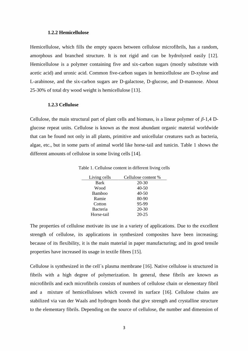
algae, etc., but in some parts of animal world like horse-tail and tunicin. Table 1 shows the

different amounts of cellulose in some living cells [14].

Table 1. Cellulose content in different living cells

Living cells Cellulose content %

Bark 20-30

Wood 40-50

Bamboo 40-50

Ramie 80-90

Cotton 95-99

Bacteria 20-30

Horse-tail 20-25

The properties of cellulose motivate its use in a variety of applications. Due to the excellent

strength of cellulose, its applications in synthesized composites have been increasing;

because of its flexibility, it is the main material in paper manufacturing; and its good tensile

properties have increased its usage in textile fibres [15].

Cellulose is synthesized in the cell´s plasma membrane [16]. Native cellulose is structured in

fibrils with a high degree of polymerization. In general, these fibrils are known as

microfibrils and each microfibrils consists of numbers of cellulose chain or elementary fibril

and a mixture of hemicelluloses which covered its surface [16]. Cellulose chains are

stabilized via van der Waals and hydrogen bonds that give strength and crystalline structure

to the elementary fibrils. Depending on the source of cellulose, the number and dimension of

4

the microfibrils varies. The diameter of the microfibrils in plants cell walls is about 3-10 nm.

However, in Valonia (an alga), Acetobacter xylinum (bacteria) and Ramie it is 18-20, 2 and

10-20 nm, respectively [17].

Four types of cellulose allomorphs have been identified: cellulose I, II, III and IV. Cellulose I

is the main type of cellulose in nature which can be found in two forms, Iα

and Iβ. Cellulose II

is the result of mercerization of cellulose I. Cellulose III is produced by treating cellulose I

and II with amines such as liquid ammonia. Cellulose IV is the product of treating cellulose I,

II, III with glycerol at high temperature. Cellulose Iα and Iβ have different crystalline forms.

Iα contains a single-chain triclinic unit cell, while Iβ

is in the form of two-chain monoclinic

unit cell [18].

There are several reports of experimental, modelling and biological studies that identified

cellulose microfibril structures [16, 19-21]. These studies show that different plant cell walls

have different crystalline structures. In most of the proposed models, cellulose is assumed to

organize the crystalline core structure that interacts with hemicellulose which forms the

noncrystalline sheath.

Figure 2 shows four proposed crystal structures for plant cell walls of cabbage and onion (a),

pineapple (b), apple cell walls (c) and Italian raygrass (d).

(a) (b) (c) (d)

Figure 2. Order of cellulose chains in cabbage and onion (a), pineapple (b), apple cell wall (c) and

Italian raygrass (d) cell walls.

Model (a) shows the order of 18 cellulose chains in cabbage and onion, containing 33%

crystalline core chains (i.e., the chains that are not on the surface) while model (b) belongs to

pineapple cell wall with 22 cellulose chains, containing 36% crystalline core chains [21]. The

models for apple cell walls (c) and Itallian raygrass (d) contain 23 and 28 cellulose chains

with about 39 and 43% of core crystallinity, respectively. It is believed that the crystalline

part of cellulose may be affected by the non-cellulosic materials present in the cell. Due to

5

the wide variety of non-cellulosic materials in different plants, the crystallite cellulose can

have different dimensions [16, 19, 21].

The studies presented in this thesis are based on a new model proposed for cellulose Iβ by

Ding and Himmel in 2006 [16, 22]. In their model 36-cellulose chains are arranged in three

layers as shown in Figure 3(a). Six crystalline core chains are surrounded by 12 sub-

crystalline chains and 18 non-crystalline chains support them in the outer layer, in which the

chains are fixed by hydrogen bonds (O3´- O5 and O2- O6´).

(a)

(b)

(c) (d)

Figure 3. Illustration of a cellulose microfibril containing 36 cellulose chains (a), numbering of the

cellulose chains in the crystalline structure of cellulose (b), cellobiose (syn) (c) and glucose (d)

molecules.

Each cellulose chain is a linear polymer of β-1,4 D-glucose repeat units. Cellobiose is the

shortest cellulose chain with two glucose repeat units. These structures are shown in Figures

3 (c) and (d).

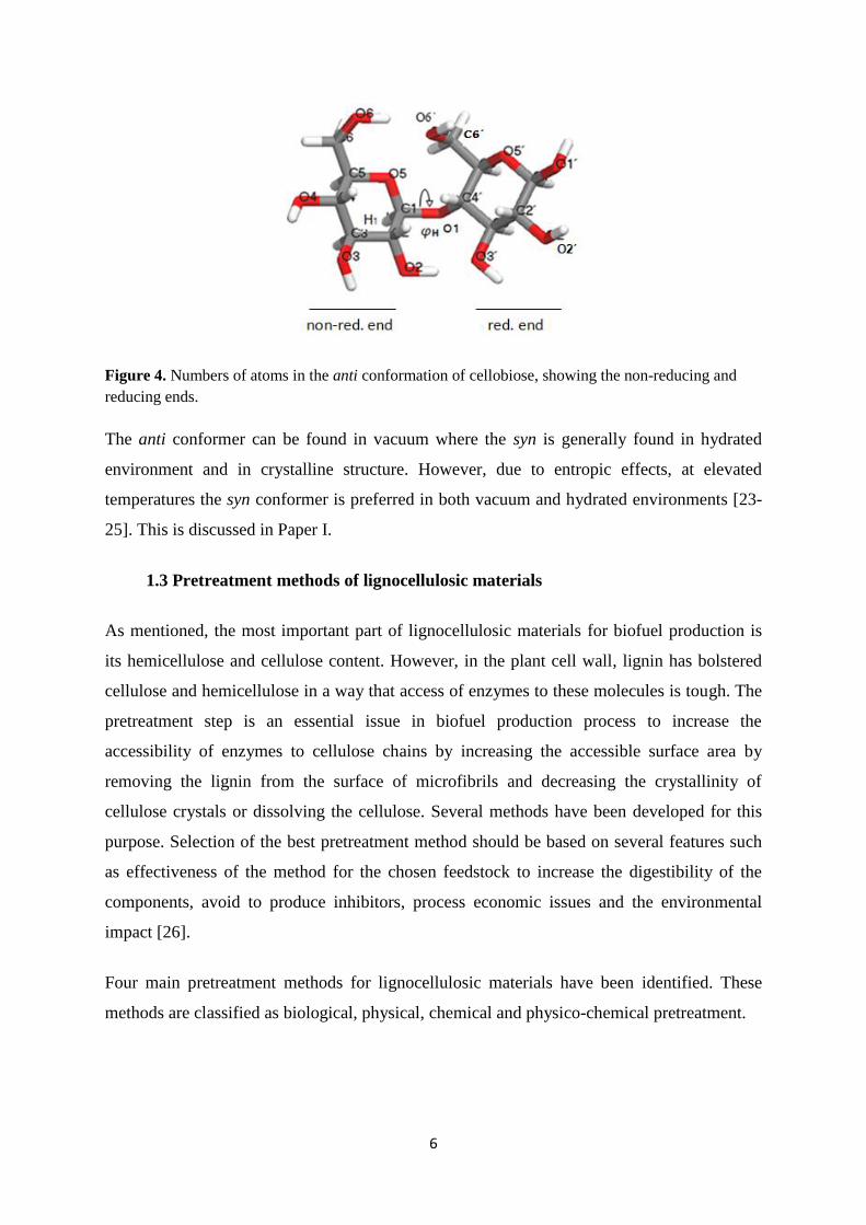
Two conformers are known for cellobiose: syn and anti. Figures 3(c) and 4 show the syn and

anti conformer of cellobiose. Numbering of atoms of cellobiose anti is also showed in Figure

4; H is torsion angle between atoms H1-C1-O-C4´. In the anti conformer, H either ψH (C1-

O-C4´-C5´) lies near -180° [23].

6

Figure 4. Numbers of atoms in the anti conformation of cellobiose, showing the non-reducing and

reducing ends.

The anti conformer can be found in vacuum where the syn is generally found in hydrated

environment and in crystalline structure. However, due to entropic effects, at elevated

temperatures the syn conformer is preferred in both vacuum and hydrated environments [23-

25]. This is discussed in Paper I.

1.3 Pretreatment methods of lignocellulosic materials

As mentioned, the most important part of lignocellulosic materials for biofuel production is

its hemicellulose and cellulose content. However, in the plant cell wall, lignin has bolstered

cellulose and hemicellulose in a way that access of enzymes to these molecules is tough. The

pretreatment step is an essential issue in biofuel production process to increase the

accessibility of enzymes to cellulose chains by increasing the accessible surface area by

removing the lignin from the surface of microfibrils and decreasing the crystallinity of

cellulose crystals or dissolving the cellulose. Several methods have been developed for this

purpose. Selection of the best pretreatment method should be based on several features such

as effectiveness of the method for the chosen feedstock to increase the digestibility of the

components, avoid to produce inhibitors, process economic issues and the environmental

impact [26].

Four main pretreatment methods for lignocellulosic materials have been identified. These

methods are classified as biological, physical, chemical and physico-chemical pretreatment.

7

The main goal of biological pretreatment is degrading of lignin. Microorganisms such as

some bacteria, and fungi such as white-, brown- and soft-rot fungi can degrade lignin and

make hemicellulose more soluble. However, the rate of cellulose dissolution is slow [27].

Physical pretreatment includes different methods such as milling (ball milling, hammer

milling, vibro energy milling, colloid milling and two-roll milling), ultrasound and irradiation

methods (gamma-ray, electron-beam and microwave irradiation), hydrothermal methods,

expansion, extrusion and pyrolysis to reduce the particle size and crystallinity [26, 28].

During chemical pretreatment, several chemicals such as sodium hydroxide, ammonia,

sulphuric acid, phosphoric acid, sulphur dioxide, hydrogen peroxide and ozone are used to

disrupt biomass structure through chemical reactions [26, 29].

The most important processes of physico-chemical pretreatment are steam explosion,

ammonia fiber explosion (AFEX), N-Methylmorpholine N-oxide (NMMO), supercritical

carbon dioxide (SC-CO2) explosion, SO2

explosion and liquid hot-water pretreatment [26-

29].

A brief description of steam and SC-CO2 explosion methods that are studied in this thesis can

be found in the following sections.

1.3.1 Steam explosion

Steam explosion was developed by Mason in 1925 [30], and Babcock used it as a

pretreatment method for bioethanol production in 1932 [31]. This method is a successful and

economical method with low environmental impact that can be applied for pretreatment of

several types of lignocellulosic biomass. Steam explosion is the most effective pretreatment

method in commercial production of bioethanol from feedstock such as wheat straw [32].

Steam explosion pretreatment includes two main steps, steaming (steam loading) and

explosion. During steaming step the lignocellulosic material is subjected to high pressure

saturated steam. It is followed by a pressure drop to atmospheric pressure called the

explosion step. The process helps to remove, depolymerise and dissolve lignin and

hemicellulose into lower molecular-weight products as well as reduces the size and

crystallinity of the cellulose structure.

8

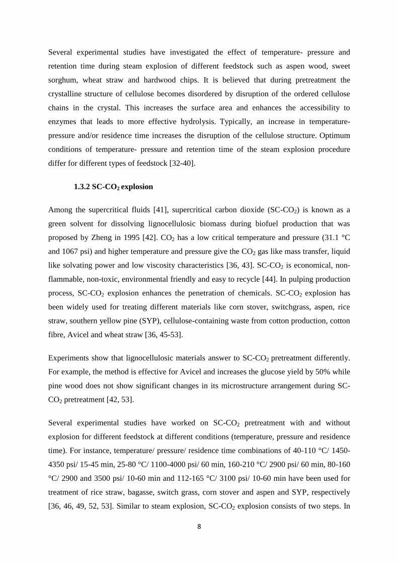
Several experimental studies have investigated the effect of temperature- pressure and

retention time during steam explosion of different feedstock such as aspen wood, sweet

sorghum, wheat straw and hardwood chips. It is believed that during pretreatment the

crystalline structure of cellulose becomes disordered by disruption of the ordered cellulose

chains in the crystal. This increases the surface area and enhances the accessibility to

enzymes that leads to more effective hydrolysis. Typically, an increase in temperature-

pressure and/or residence time increases the disruption of the cellulose structure. Optimum

conditions of temperature- pressure and retention time of the steam explosion procedure

differ for different types of feedstock [32-40].

1.3.2 SC-CO2 explosion

Among the supercritical fluids [41], supercritical carbon dioxide (SC-CO2) is known as a

green solvent for dissolving lignocellulosic biomass during biofuel production that was

proposed by Zheng in 1995 [42]. CO2 has a low critical temperature and pressure (31.1 °C

and 1067 psi) and higher temperature and pressure give the CO2 gas like mass transfer, liquid

like solvating power and low viscosity characteristics [36, 43]. SC-CO2 is economical, non-

flammable, non-toxic, environmental friendly and easy to recycle [44]. In pulping production

process, SC-CO2 explosion enhances the penetration of chemicals. SC-CO2 explosion has

been widely used for treating different materials like corn stover, switchgrass, aspen, rice

straw, southern yellow pine (SYP), cellulose-containing waste from cotton production, cotton

fibre, Avicel and wheat straw [36, 45-53].

Experiments show that lignocellulosic materials answer to SC-CO2 pretreatment differently.

For example, the method is effective for Avicel and increases the glucose yield by 50% while

pine wood does not show significant changes in its microstructure arrangement during SC-

CO2 pretreatment [42, 53].

Several experimental studies have worked on SC-CO2 pretreatment with and without

explosion for different feedstock at different conditions (temperature, pressure and residence

time). For instance, temperature/ pressure/ residence time combinations of 40-110 °C/ 1450-

4350 psi/ 15-45 min, 25-80 °C/ 1100-4000 psi/ 60 min, 160-210 °C/ 2900 psi/ 60 min, 80-160

°C/ 2900 and 3500 psi/ 10-60 min and 112-165 °C/ 3100 psi/ 10-60 min have been used for

treatment of rice straw, bagasse, switch grass, corn stover and aspen and SYP, respectively

[36, 46, 49, 52, 53]. Similar to steam explosion, SC-CO2 explosion consists of two steps. In

9

the first step, the material is subjected to high temperature and pressure CO2 (above its

critical temperature and pressure) and in the second step, the pressure drops to atmospheric

pressure rapidly. SC-CO2 explosion helps in removing, dissolving and depolymerisation of

lignin and hemicellulose into lower molecular-weight products as well as reduction of the

crystallinity of the cellulose structure.

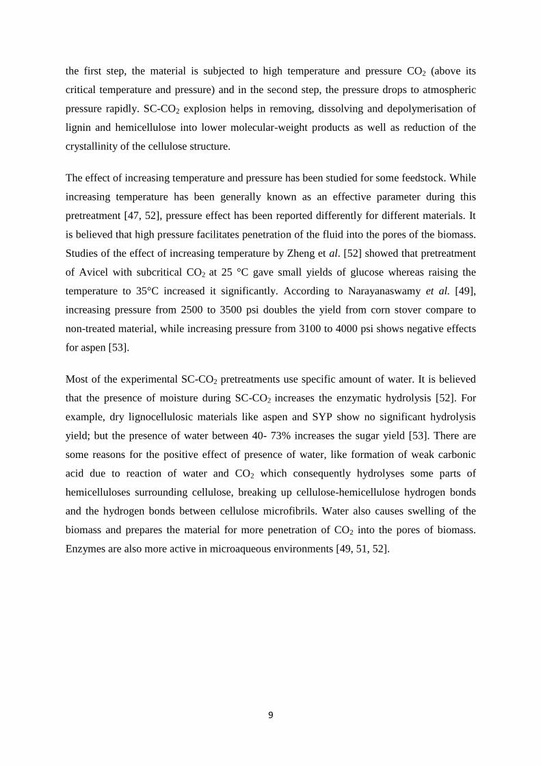
The effect of increasing temperature and pressure has been studied for some feedstock. While

increasing temperature has been generally known as an effective parameter during this

pretreatment [47, 52], pressure effect has been reported differently for different materials. It

is believed that high pressure facilitates penetration of the fluid into the pores of the biomass.

Studies of the effect of increasing temperature by Zheng et al. [52] showed that pretreatment

of Avicel with subcritical CO2 at 25 °C gave small yields of glucose whereas raising the

temperature to 35°C increased it significantly. According to Narayanaswamy et al. [49],

increasing pressure from 2500 to 3500 psi doubles the yield from corn stover compare to

non-treated material, while increasing pressure from 3100 to 4000 psi shows negative effects

for aspen [53].

Most of the experimental SC-CO2 pretreatments use specific amount of water. It is believed

that the presence of moisture during SC-CO2 increases the enzymatic hydrolysis [52]. For

example, dry lignocellulosic materials like aspen and SYP show no significant hydrolysis

yield; but the presence of water between 40- 73% increases the sugar yield [53]. There are

some reasons for the positive effect of presence of water, like formation of weak carbonic

acid due to reaction of water and CO2 which consequently hydrolyses some parts of

hemicelluloses surrounding cellulose, breaking up cellulose-hemicellulose hydrogen bonds

and the hydrogen bonds between cellulose microfibrils. Water also causes swelling of the

biomass and prepares the material for more penetration of CO2 into the pores of biomass.

Enzymes are also more active in microaqueous environments [49, 51, 52].

10

2 Computational Methods

Computational studies complement experimental studies. Computational chemistry or

molecular modelling uses a set of theories and techniques to solve chemical problems like

molecular energies and geometries, transition states, chemical reactions, spectroscopy (IR,

UV and NMR), electrostatic potentials and charges on a computer. Connection between

theory and experiment helps to a have a better understanding of vague and inconsistent

results, optimization of design or progress of chemical processes and prediction of the results

of difficult or dangerous experiments. However computational chemistry techniques are

expensive and models cannot be computed accurately and need some approximations.

Computational chemistry is based on classical and quantum mechanics and covers a wide

range of areas like statistical mechanics, cheminformatics, semi-empirical methods,

molecular mechanics and quantum chemistry. Various methods have been developed to study

the structures and the energies of molecules, either using quantum mechanics or molecular

mechanics. Due to its cost, quantum mechanics can be used for small molecules or systems

containing with a good accuracy while molecular mechanics can be applied to larger systems

containing thousands of atoms [54].

In the following paragraphs a brief description of the methods that have been used in this

thesis is given.

2.1 Quantum mechanics

Quantum mechanics describes the behaviour of the electrons mathematically and describes

electron density using a wave function, Ψ(r). Quantum mechanics is based on the time-

independent Schrödinger equation (Eq.1):

H(r) Ψ(r) = E(r) Ψ(r) Eq. 1

where H(r) is the Hamiltonian operator, Ψ(r) is the wave function and E(r) is the total energy

(kinetic and potential) of the system and r denotes the nuclear and electronic positions [55,

56]. When no external field is present, the Hamiltonian operator is given by factors related to

interaction of electrons, interaction of nuclei and interaction between electrons and nuclei

according to Eq. 2:

11

∑

∑ ∑

∑

∑

∑

Eq. 2

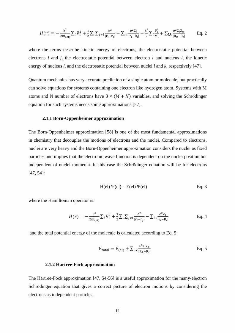
where the terms describe kinetic energy of electrons, the electrostatic potential between

electrons i and j, the electrostatic potential between electron i and nucleus l, the kinetic

energy of nucleus l, and the electrostatic potential between nuclei l and k, respectively [47].

Quantum mechanics has very accurate prediction of a single atom or molecule, but practically

can solve equations for systems containing one electron like hydrogen atom. Systems with M

atoms and N number of electrons have variables, and solving the Schrödinger

equation for such systems needs some approximations [57].

2.1.1 Born-Oppenheimer approximation

The Born-Oppenheimer approximation [58] is one of the most fundamental approximations

in chemistry that decouples the motions of electrons and the nuclei. Compared to electrons,

nuclei are very heavy and the Born-Oppenheimer approximation considers the nuclei as fixed

particles and implies that the electronic wave function is dependent on the nuclei position but

independent of nuclei momenta. In this case the Schrödinger equation will be for electrons

[47, 54]:

H(el) Ψ(el) = E(el) Ψ(el) Eq. 3

where the Hamiltonian operator is:

∑

∑ ∑

∑

Eq. 4

and the total potential energy of the molecule is calculated according to Eq. 5:

∑

Eq. 5

2.1.2 Hartree-Fock approximation

The Hartree-Fock approximation [47, 54-56] is a useful approximation for the many-electron

Schrödinger equation that gives a correct picture of electron motions by considering the

electrons as independent particles.

12

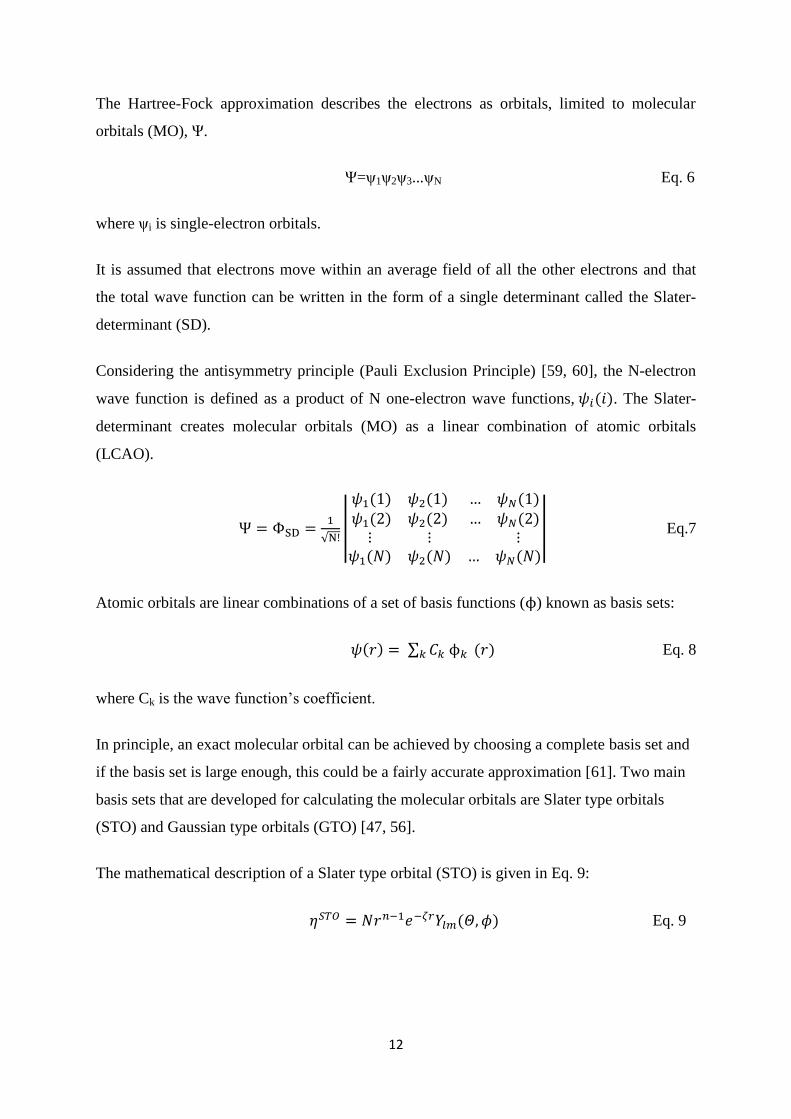
The Hartree-Fock approximation describes the electrons as orbitals, limited to molecular

orbitals (MO), Ψ.

Ψ=ψ1ψ2ψ3...ψN Eq. 6

where ψi is single-electron orbitals.

It is assumed that electrons move within an average field of all the other electrons and that

the total wave function can be written in the form of a single determinant called the Slater-

determinant (SD).

Considering the antisymmetry principle (Pauli Exclusion Principle) [59, 60], the N-electron

wave function is defined as a product of N one-electron wave functions, . The Slater-

determinant creates molecular orbitals (MO) as a linear combination of atomic orbitals

(LCAO).

√ |

| Eq.7

Atomic orbitals are linear combinations of a set of basis functions (ϕ) known as basis sets:

∑ ϕ Eq. 8

where Ck is the wave function’s coefficient.

In principle, an exact molecular orbital can be achieved by choosing a complete basis set and

if the basis set is large enough, this could be a fairly accurate approximation [61]. Two main

basis sets that are developed for calculating the molecular orbitals are Slater type orbitals

(STO) and Gaussian type orbitals (GTO) [47, 56].

The mathematical description of a Slater type orbital (STO) is given in Eq. 9:

Eq. 9

13

where N is a normalization factor, n is the quantum number, ζ corresponds to the orbital

exponent, r is the radius and Ylm describes the angular part of the function. However,

Gaussian type orbitals (GTO) is given as the mathematical form in Eq. 10:

Eq.10

where N is a normalization factor, α corresponds to the orbital exponent, r is the radius and l,

m, n are quantum numbers such that L= l+ m+ n gives the angular momentum of η. A linear

combination of Gaussian functions or “Contracted Gaussians” (CGs) in the form of STO-MG

are widely used that approximate Slater-type orbitals (STOs) by M primitive Gaussians

(GTOs). STO-3G is called a “minimal basis set”, that is simplest possible atomic orbital that

has the lowest basis functions.

Extending the basis sets is possible by adding the double zeta, triple or quadruple zeta to the

basis sets, so that the set of functions are doubled, tripled or quartet. Split-valence basis sets

apply two or three more basis functions to each valence orbital. Addition of polarization (*)

and diffusion (+) functions to the basis sets can extend the basis sets even more. Polarization

functions add orbitals higher in energy than the valence orbitals of each atom, e. g., adding

the p-functions for hydrogen or d-functions for the first-row elements of the periodic table.

Diffusion functions allow the electrons to be distributed far from the ionic positions. This

function is useful for description of systems where the electrons need to move far from

nuclei, like anions [62].

Hartree-Fock is a molecular orbital approximation that gives a set of coupled differential

equations but cannot explain the correlation between electrons. It gives good description for

many equilibrium geometries in the ground state but cannot describe thermochemistry where

bonds are broken or formed. Using adequate basis sets, Hartree-Fock wave function can

predict 99% of the total energy where the 1% remaining energy belongs to correlation

interactions between electrons. The post-Hartree-Fock methods and Density Functional

Theory (DFT) are useful methods that give more flexibility to Hartree-Fock methods. The so-

called second-order Møller-Plesset model (MP2) is a commonly used method that describes

thermochemistry where bonds are broken or formed [56].

14

2.1.3 Post-Hartree-Fock methods

Configuration interaction (CI) [63] and Møller-Plesset (MP) [64] are two of the useful

methods that improve the flexibility of the Hartree-Fock through mixing the ground-state

wave functions with excited-state wave functions. They also give a good description of

electron correlations. However they are more expensive than Hartree-Fock methods. The

correlation energy (EC) is the difference between the real energy of the molecule and the

energy calculated by Hartree-Fock methods.

Eq. 11

MP methods are based on perturbation theory. Simply, the Møller-Plesset model mixes

ground-state and excited-state wave functions together, i.e. when MP2 is applied, one or two

electrons from occupied orbitals in the Hartree-Fock configuration will move to the

unoccupied orbitals (excited state) to calculate the contribution to the correlation energy.

Different orders of MP methods give different description of electronic structures. If MP0

considers electron repulsion in one molecular orbital, MP1 can be regarded as the Hartree-

Fock wave function, considering an average of inter-electronic repulsions [64]. Higher orders

of MP by addition of more functions can improve the calculations and give more accurate

correlation energies but require large computational resources. MP2 methods account for ~

80-90% of the correlation energy, while higher orders of MP like MP3 and MP4 account for

~ 90-95% and ~ 95-98%, respectively [56, 65].

2.1.4 Density Functional Theory (DFT)

DFT [47, 66] is first principles method based on the electron density ρ(r), Eq. 12,

∫ ∫ ( )

Eq. 12

where Nel denotes the total number of electrons.

The idea of DFT theory was born in the late 1920s by Thomas-Fermi model, but the density

functional theory as we know it today was introduced in the contributions by Hohenberg-

Kohn (1964) and Kohn-Sham (1965). DFT methods can be applied to larger systems than the

post-Hartree-Fock methods. Hohenberg and Kohn showed that properties and the ground

15

state energy of a system can be defined solely by the electron density [67]. In DFT method,

energy functional can be calculated as Eq. 13:

[ ] ∫ [ ] Eq. 13

where Vext (r) is the external potential due to the Coulomb interaction between electrons and

nuclei, and F[ρ(r)] is kinetic energy of the electrons and the energy obtained from interaction

of electrons. The problem with this definition was that the function F[ρ(r)] was not clear; one

year later Kohn and Sham extended the equation to Eq. 14 :

[ ] [ ] [ ] [ ] Eq. 14

in which EKE[ρ(r)] is kinetic energy of non-interacting electrons , EH[ρ(r)] is Coulombic

energy between electrons and EXC[ρ(r)] is the energy due to exchange and correlation. The

kinetic energy of non-interacting electrons, EKE [ρ(r)], can be obtained according to Eq. 15:

[ ] ∑ ∫ (

) Eq. 15

EH[(ρ)] or Hartree electrostatic energy, which is the electrostatic energy due to interaction

between charge densities, is given in Eq. 16 :

[ ]

∬

Eq. 16

Considering the Coulomb interaction between electrons and nuclei, Vext(r), Eq. 13 can be

written as:

[ ] ∑ ∫ (

)

∬

[ ]

∑ ∫

Eq. 17

where M is the number of ions in the system.

The exchange-correlation functional, EXC [ρ(r)], is developed by several approaches. The

simplest one is the Local Density Approximation (LDA) [47, 68, 69] which states that

exchange-correlational energy is only affected by the local electron density and is given by

Eq. 18:

16

[ ] ∫ ( ) Eq. 18

(ρ) can be obtained from simulations of a homogeneous electron gas.

Adding electron spins 𝛼 and β to Eq. 18 yields a modified version of LDA called Local Spin

Density approximation (LSD):

[ ] ∫ ( ) Eq. 19

An improved method beyond LDA is Generalized Gradient Approximation (GGA) [47, 70]

which includes both local electron density and the gradient of the charge density. The

gradient term shows the rate of density changes and is known as non-local functional.

[ ] ∫ ( ) Eq. 20

PW91 [71] and PBE [70] are two general GGA functionals. Further improvement to the GGA

is possible by including a certain amount of Hartree-Fock (HF) exchange. These functionals

are known as hybrid functionals [72]. One of the most popular functionals, that has been used

in the calculations presented here, is B3LYP (Becke three-parameter exchange and the Lee–

Yang–Parr correlation functionals) [73-76] that includes LSD, Hartree-Fock and Becke (B)

exchange functionals and LSD and Lee-Yang-Parr (LYP) correlation functionals [47]:

Eq. 21

a, b and d are equal to 0.2, 0.72 and 0.81, respectively; the values are fitted to the empirical

data like atomization energies, ionization potentials and proton affinities.

Nowadays, Kohn-Sham-DFT is one of the most common methods for calculating electronic

structures of molecules in quantum chemistry, but one of the main challenges for DFT is its

deficiency to find a correct description of dispersion interactions for long-range van der

Waals forces. Many approaches have been proposed for the inclusion of dispersion

interactions [77-79] [67]. One of the useful methods is DFT-D with B3LYP and PBE

functionals that was developed by Grimme:

Eq. 22

17

where is an empirical dispersion correction including an energy term of the

:

∑ ∑

Eq. 23

N is the number of atoms, is the dispersion coefficient for ij atom pair, is the global

scaling factor that depends on the DFT method and is the distance between atoms i and j.

When the sum of van der Waals radii is Rr, the damping function is given by:

( )

⁄ Eq. 24

In this thesis, the DFT-D method has been used in the Papers IV and V.

2.2 Molecular Mechanics

Molecular mechanics (MM) is widely used for conformational analysis. It is less accurate but

more economical than quantum mechanics methods and can be applied to large systems like

organic materials (oligonucleotides, hydrocarbons and peptides) and in some cases to

metallo-organics and inorganics. In molecular mechanics, there is no reference to electrons

and molecules are considered as a collection of balls joined by springs; the energy of a

system (Eq. 25) caused by the geometry of the molecules in terms of a sum of contributions

of bonding (stretching, bending, torsion and inversion) and non-bonding (electrostatic and

van der Waals) energies between atoms [80, 81].

Eq. 25

These energy terms are illustrated in Figure. 5:

Figure 5- Schematic view of contributions of stretching, bending, torsion, inversion and non-bonding

energies in a molecule

18

Molecular mechanics uses a set of mathematical functions that are so-called force fields to

describe the potential energy of molecular systems, thus generally molecular mechanics

methods denoted as force field methods [56, 65]. The parameters of force field functions are

fitted to both quantum mechanics and empirical data to describe entire types of atoms in the

molecules; hence the choice of the molecular model and the force field is an essential step in

prediction of the geometry and conformation of the molecules. Several groups of force fields

have been developed for this purpose; classical force fields, second-generation force fields,

special-purpose force fields and rule-based force fields are main groups of force fields [82].

Molecular mechanics employs one or more minimization method to find the local minima on

the potential energy surface (PES). Steepest descent [83], conjugate gradient [84] and

Newton-Raphson [85] are a number of well-known algorithms that are mostly used by

molecular mechanics to find the geometry of the structure related to the local minima [65].

Three force fields, COMPASS, Dreiding and Universal that are applicable for polymers have

been used in this thesis and will be discussed briefly. The COMPASS force field belongs to

second-generation force fields while Dreiding and Universal (UFF) fit in the Rule-based

force fields.

2.2.1 COMPASS force field

COMPASS (Condensed-phase Optimized Molecular Potentials for Atomistic Simulation

Studies) [86] is an ab initio force field that is based on the PCFF (Polymer Consistent Force

Field) [87]. The COMPASS force field gives good prediction of geometry, conformational,

vibrational, and thermophysical properties of a broad range of molecules, especially polymers

in both isolation and condensed phases [88].

The COMPASS force field potential energy expression is given in Eq. 26. The first four

terms account for bond stretch, angle bend, out-of-plane torsion and out-of-plane wag

energies, terms five to ten are for cross-coupling and the last two terms show electrostatic

interactions and van der Waals energies, respectively.

19

∑[

] ∑[

] ∑

] ∑

∑

∑

∑

∑

[ ] ∑

[ ] ∑

∑

∑

[ ⁄ ⁄ ]

Eq. 26

b, θ, and γ are bond length, angle, torsion angle and out-of-plane wag or inversion angle,

respectively, Qi and Qj are atomic charges and Rij is the interatomic separation. Parameters of

b0 and θ0 are equilibrium values and K and K1- K3 are constants. However parameters for the

intramolecular terms as well as the atomic charges have been fit to ab initio data, and those

for the intermolecular terms are fit to empirical data [86, 89].

2.2.2 Dreiding force field

The Dreiding force field [90] has been fitted to biological, organic and some inorganic

molecules where atomic hybridization has been considered when fitting the parameters and

force constants. The Dreiding force field calculates the potential energy by considering

bonded energy i.e., bond stretch, angle bend, out-of-plane torsion and inversion (out-of-plane

wag angle), and non-bonded energy i.e. electrostatic interactions, the Van der Waals

interactions and hydrogen bond energies. For calculation of bond stretch energy, in some

applications harmonic functions can be replaced by Morse functions that are more accurate

[91, 92]. The van der Waals interactions are based on the Lennard-Jones potential. Hydrogen

bond energy is calculated according to Eq. 27:

[ ⁄ ⁄ ] Eq. 27

20

De is the energy for bond dissociation; Re is equilibrium distance and RDA is the length

between electron donor and acceptor atoms. ӨDHA is the bond angle between atoms A, D and

H (hydrogen) [90].

2.2.3 Universal force field

The Universal force field (UFF) [91] is a biological force field which can cover the entire

elements of the periodic table. This force field is reasonably precise for geometry estimation

and energy calculation of organic conformers, metal complexes and organo-metalic

molecules. The Universal energy expressions are the sum of bonding and non-bonding

energies. Like Dreiding, both harmonic oscillator and Morse functions can be used for

calculation of bond stretch energy. Angular bend is given by General Fourier extension and

inversion term is according to Cosine Fourier expansion. Non-bond interactions are

introduced as van der Waals (Lennard-Jones potential) and electrostatic interaction [91].

In brief, molecular mechanics is a rapid and simple force field based method that can be

applied for systems comprising several thousand atoms but is limited to finding particular

conformation in equilibrium state. However, it is not able to explain the transition state and

time evolution of the system.

2.3 Molecular Dynamics

Molecular dynamics focuses on molecules in motion through the study of nuclear motions by

step-by-step solving the Newton’s equation of motion (Eq. 28) to calculate the trajectory of

all atoms [55, 65, 93]:

Eq. 28

where Fi is the force acting on particle i at time t, mi is the mass of the particle and ri is the

position vector of i th particle. The trajectories show the position, velocity and acceleration of

the particles in the system under a period of time. Choosing an adequate time step is needed

to have an acceptable time evolution. A too short time step is very expensive and covers a

limited phase space, but a big time step makes the system unstable and leads to errors. In

molecular dynamics, parameters like positions, velocities and also accelerations are often

approximated as Taylor expansion (Eq. 29) and (Eq. 30) using time step δt:

21

Eq. 29

[ ] Eq. 30

ri shows the position, vi stand for velocity and ai is acceleration of particle i. An integrator is

needed to project the trajectory over a small time step [93]. There are several integrators

for this purpose like the Verlet, Verlet leap frog, Gear fixed time step, Gear variable time

step, Runge-Kutta, and Gauss-Radau algorithms [94]. The Verlet algorithm (Eq. 31) is a

time-reversible algorithm [95] that, because of its simplicity and stability, is a widely used

integration algorithm:

Eq. 31

and the velocity will be:

[ ] Eq. 32

In brief, in MD simulation, calculating time evolution is performed by numerically

integrating Newton´s equation of motion for interacting atoms.

Molecular dynamics describes the potential energy of molecules by using an appropriate

molecular mechanics force field. Choosing an ensemble such as NVT, NpT or NVE will

identify which parameters are constant during the simulation. NVT keeps the number of

particles, volume and temperature constant, while in NpT the number of particles, pressure

and temperature remain unchanged and in NVE as well as the number of particles and

volume, energy is kept constant too. NVT, NpT and NVE ensembles have been used in this

thesis for study of steam and SC-CO2 explosion.

2.4 Monte Carlo methods

Monte Carlo (MC) is a stochastic method based on probabilities, where random numbers are

used to create a sequence of possible configurations.

In the MC methods, the particles can be positioned, for example, by transition between

points, or random insertion-deletion of particles. The new conformations are then accepted or

22

rejected according to some filter. Many states are generated, and the energy of each

conformation is calculated, often using a molecular mechanics force field.

However random numbers decide how atoms or molecules move to generate new

conformations or geometric arrangements. In other words, configurations are chosen

randomly and then their impact is weighted with exp(− /kBT), where ∆E is the energy

difference between two configuration, kB is Boltzman constant and T is temperature.

Metropolis method is a development of Monte Carlo method [96]. According to this method,

configurations are chosen with a probability distribution of exp(− /kBT) and then weighted

equally.

Simply, if i is the configuration of a system of particles, the Metropolis Monte Carlo

algorithm generates a new configuration j with a transition probability of P(i→ j):

⁄ ) Eq. 33

where ∆Eij is the energy difference between configuration i and j. If the energy of the new

configuration j is lower than the old one (i), i.e., ∆Eij ≤ 0, the new configuration j is accepted

for the new positioning; but if j has a higher energy than i or ∆Eij > 0, P(i→ j) is compared to

a random number ζ where 0< ζ< 1; if P(i→ j) > ζ, the new configuration is accepted,

otherwise j is rejected and a new configuration is generated [55, 56, 65, 97].

Metropolis Monte Carlo is a faster method with high quality of the statistics that ensures that

accepted structures have a Boltzmann distribution. However, the magnitude of the particle

displacements should be selected carefully, since a small change in displacement leads to

high acceptance, but is a slow procedure. However big change is faster but the probability of

acceptance is lower and the number of sampled configurations is few [56].

Grand canonical Monte Carlo (GCMC) simulation is an appropriate tool to, for example,

study physical interactions of fluids with solid systems. An example is when one simulates a

solid sorbent phase and a liquid or gas phase at equilibrium with a specified chemical

potential [98].

In grand canonical Monte Carlo, which has a partition function denoted by Ξ (µ, V, T), the

volume, temperature and chemical potential are conserved. The system is open and the

23

numbers of particles are allowed to fluctuate by discontinuously creating new particles and

destroying them during the simulation. This helps to minimize ergodic difficulties of the

system.

In the grand canonical ensemble, the probability of a configuration m, is given by Eq. 34:

[ ] Eq. 34

where C is an arbitrary normalization constant,

, Em is the total energy of

configuration m, and the function F(N) is calculated by Eq. 35:

(

) Eq. 35

where, is the fugacity, is the intramolecular chemical potential and N is the loading of

the component. Probability of accepting the proposed configuration n is then calculated

according to Eq. 36:

[

] Eq. 36

24

3 Summary of Papers I-V

Molecular–level studies of dissolution of crystalline structure of cellulose during steam and

supercritical carbon dioxide (SC-CO2) were performed using grand canonical Monte Carlo

and molecular dynamics. For both simulations, COMPASS force field was used. The validity

of this force field for these systems was tested by comparing the energy and structures

obtained from quantum and molecular mechanics. These studies are presented in Papers I to

V.

Quantum mechanics calculations were performed in the GAUSSIAN 09 program package at

Neolith, AKKA and C3SE, and GAMESS-US program at the high performance computer

cluster Kalkyl at UPPMAX. Molecular mechanics, Monte Carlo and molecular dynamics

calculations were performed using the Materials Studio package version 6.0 (Accelrys

Software Inc).

3.1 Papers I & II

Paper I presents the results from the COMPASS, Dreiding and Universal force fields for

studies of cellulose systems. These force fields are widely used for studies of polymeric

systems. The validity of the force field is tested by comparing structures and energies

obtained by the force fields with data obtained from first principles calculations. The use of

first principles methods requires that the comparison is limited to small systems of

importance to cellulose, and we therefore focus on glucose and cellobiose molecules as well

as their interaction with water molecules. The results indicate that the COMPASS force field

is preferred over the Dreiding and Universal force fields for studying dissolution of large

cellulose structures.

Figure 6 illustrates the annealed structure of cellobiose obtained from each of the three force

fields, as well as the corresponding structures obtained after B3LYP/6-311++G**

minimization. Similar structures are obtained after geometry optimization with the other DFT

and MP2 calculations. It is clear that the annealed (and first principles optimized) cellobiose

structure depends on the force field used for the annealing. The annealed structures obtained

from COMPASS did not show significant change during the subsequent optimization with

the first principles methods. For example, when performing geometry optimization with

B3LYP/6-311++G** the bond lengths changed by less than 0.02 Å and the change in bond

25

angle was less than 2 degrees. The cellobiose structure obtained from Dreiding shows a larger

change during the subsequent optimization with DFT (where an OH group rotates).

Cellobiose structures obtained from Universal also show large changes during DFT geometry

optimization. Together with the relative energies of the first principles methods discussed

below with respect to Table 2, this indicates that the COMPASS force field yields the

preferred cellobiose structures.

Figure 6- Cellobiose molecular structures (top and side view) obtained after annealing with the

COMPASS, Dreiding and Universal force fields (upper three figures) and after further geometry

optimization with B3LYP/6-311++G**.

The three force fields yield different structures for the cellobiose molecule. Figure 6 also

shows that there is a large difference in the cellobiose structures obtained from the different

force fields. Dreiding and Universal force fields yield syn structures whereas COMPASS

yields an anti structure. The torsions are φH =30.1° (φH is defined in Figure.4) for the

Dreiding force field, φH =51.4° for the Universal force field and φH = -179° for the

COMPASS force field. More structural details like torsion angles that exemplify differences

in the structures can be found in appended Papers I and II.

26

Relative energies of the cellulose molecules that were optimized using the different quantum

mechanics methods and basis sets are listed in Table 2. The energies in columns 3, 4 and 5

are obtained when the initial glucose structure is from the COMPASS, Dreiding and

Universal force fields, respectively.

Table 2- Relative energies (kcal/mol) for the cellobiose molecule obtained after geometry

optimization with the first principles methods. Energies are given relative to the results obtained when

the initial structure is from the COMPASS force field. ‡

These results are from MP2/6-

311++G**//B3LYP/6-311++G** calculations.

Method Basis-set Initial structure from

COMPASS Initial structure from

Dreiding Initial structure from

Universal

MP2 6-311G 0.0 10.3 11.7

6-311G** 0.0 9.3 8.5

‡ 6-311++G** 0.0 7.7 8.2

B3LYP

6-311G 0.0 8.6 11.0

6-311G** 0.0 6.9 11.6

6-311++G** 0.0 5.1 5.0

PBE

6-311G 0.0 9.3 11.5

6-311G** 0.0 7.3 12.3

6-311++G** 0.0 5.4 6.2

B3PW91 6-311G 0.0 8.7 10.7

6-311G** 0.0 6.8 11.1 6-311++G** 0.0 5.2 5.7

Table 2 also shows that all methods and basis sets yield the lowest energy for the cellobiose

structure that was obtained from annealing using the COMPASS force field. There is a

rather large energy difference between the structures obtained from the various force fields.

For example, the B3LYP/6-311++G** energy from the COMPASS structure is 5.1 and 5.0

kcal/mol lower than the structures obtained from the Dreiding and Universal force fields,

respectively.

This conclusion is also supported by comparing the energies of the structures optimised by

B3LYP. The energies of the cellobiose structures that are geometry optimised using B3LYP

and when starting with structures obtained after annealing with the COMPASS, Dreiding

and Universal force fields are -814729.84, -814724.72 and -814724.83 kcal mol-1

,

respectively. Hence, the cellobiose structure obtained from the COMPASS force field not

only has a structure that is in good agreement with B3LYP, but it is also the energetically

preferred structure.

27

Similar results were obtained for glucose structures. All first principles methods and basis

sets yield the COMPASS structure as the lowest energy structure that can be found in the

original appended Paper. This indicates that COMPASS is the preferred force field when

studying the glucose and cellobiose molecule.

Since the COMPASS force field is preferred, it was used in a more detailed comparison for

the cellobiose molecule hydrated with between 0 and 4 water molecules. The comparison was

made with relative energies and structures calculated using the B3LYP/6-311++G** method

that were initially geometry optimized using AMB02C empirical force field. The COMPASS

force field yields results for cellobiose that are in excellent agreement with these DFT results.

The quantitative agreement seen for cellobiose deteriorates as more water molecules are

added to the system.

According to previous studies, the syn conformers have a larger entropy contribution than the

anti conformers, and may therefore be thermodynamically stable at higher temperatures. MD

simulations at various temperatures under NpT conditions at 1 bar showed that at very low

temperatures (e.g., 100 K) the conformer that is observed in the simulations depends on the

initial cellobiose structure; i.e., the syn (anti) conformer is seen when starting with the syn

(anti) structure since the energy barrier for isomerization has not been passed within the

simulation time. However, this is not the case for higher temperatures.

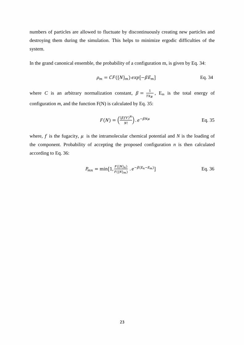
Figure 7 shows the distribution of φH when the cellobiose (in vacuum) initially had a syn

conformation and the temperature is 298 K. The data shown in the figure were obtained from

the last part of the simulation, once the syn had isomerized to anti. Note that the same results

were obtained at 325 K, and in neither case did the anti revert back to the syn. Hence, at these

temperatures the anti conformer is thermodynamically stable.

28

Figure 7- Torsion distribution, φH, of cellobiose in vacuum at 298 K when the initial structure is syn.

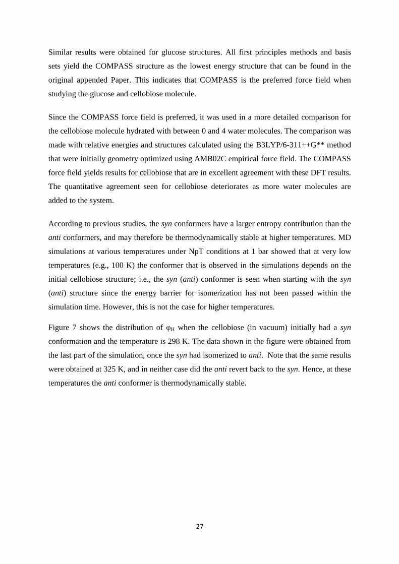
Figure 8 shows that the anti conformation remains in this conformation at 298 K, which is

expected since this is the thermodymically stable structure. However, at 375 K there are

peaks in the distribution that belong to both anti and syn conformations. It is important to

note that multiple barrier crossings occur, i.e., many anti ↔ syn isomerisation occur in the

simulation time) showing that both parts of coordinate space are sampled at this temperature.

As expected, the same behaviour is found at even higher temperatures, with the fraction of

time spent in the syn conformation increasing with temperature. This trend does not depend

on which initial conformer is used.

Figure 8- Torsion distribution, φH, of cellobiose in vacuum at 298K and 375 K when the initial

structure is anti.

0 .0 0 0

0 .0 1 0

0 .0 2 0

0 .0 3 0

0 .0 4 0

0 .0 5 0

0 .0 6 0

0 .0 7 0

-180 0 180

298 K

Re

lative

P

rob

ab

ility

φH (Torsion distribution)

0 .0 0

0 .0 1

0 .0 2

0 .0 3

0 .0 4

0 .0 5

0 .0 6

0 .0 7

-180 0 180

298 K

0 .0 0

0 .0 1

0 .0 2

0 .0 3

0 .0 4

0 .0 5

0 .0 6

0 .0 7

-180 0 180

375 K

Rel

ativ

e P

roba

bilit

y

φH (Torsion distribution)

29

The distributions of φH for cellobiose in bulk water at 1 bar and 100, 298, 350 and 475 K are

shown in Fig. 9.

Figure 9- Torsion distribution, φH, of cellobiose in bulk water at 100, 298, 350 and 475 K, when the

initial structures are syn (left) and anti (right).

The COMPASS force field was also used to study the binding strength between two parallel

glucose and two parallel cellobiose molecules. This binding strength is expected to be

important when dissolving cellulose in a pretreatment process. The glucose-glucose and

cellobiose-cellobiose structures obtained from annealing with the COMPASS force field are

Re

lative

P

rob

ab

ility

φH (Torsion distribution)

0 .0 0

0 .0 2

0 .0 4

0 .0 6

0 .0 8

0 .1 0

0 .1 2

-180 180

1

100 K

0 .0 0

0 .0 2

0 .0 4

0 .0 6

0 .0 8

0 .1 0

0 .1 2

-1 8 0 1 8 0

298 K

0 .0 0

0 .0 2

0 .0 4

0 .0 6

0 .0 8

0 .1 0

0 .1 2

-1 8 0 1 8 0

350 K

0 .0 0

0 .0 2

0 .0 4

0 .0 6

0 .0 8

0 .1 0

0 .1 2

-180 0 180

475 K

0. 00

0. 02

0. 04

0. 06

0. 08

0. 10

0. 12

- 180 180

1

100 K

0. 00

0. 02

0. 04

0. 06

0. 08

0. 10

0. 12

- 180 180

350 K

0. 00

0. 02

0. 04

0. 06

0. 08

0. 10

0. 12

-180 0 180

4

475 K

Re

lative

P

rob

ab

ility

0. 00

0. 02

0. 04

0. 06

0. 08

0. 10

0. 12

1 3 5 7 9 11 13 15 17 19 21 23 25 27 29 31 33 35 37 39 41 43 45 47 49 51 53 55 57 59 61 63 65 67 69 71 73 75 77 79 81 83 85 87 89 91 93 95 97 99 101103105107109111113115117119121123125127129131133135137139141143145147149151153155157159161163165167169171173175177179181183185187189191193195197199201203205207209211213215217219221223225227229231233235237239241243245247249251253255257259261263265267269271273275277279281283285287289291293295297299301303305307309311313315317319321323325327329331333335337339341343345347349351353355357359361

298 K

φH (Torsion distribution)

30

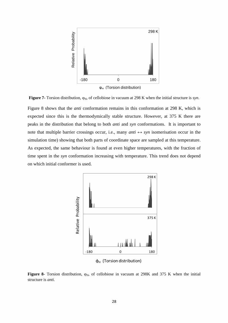
shown in the left column of Figure 10, and the structures after further geometry optimisation

with B3LYP/6-311++G** are shown in the right column. There is very little change in the

structure after geometry optimisation. For example, the glucose-glucose and cellobiose-

cellobiose centre of mass distances are 5.16 and 4.52 Å after annealing, and they change to

5.36 and 4.31 Å after geometry optimisation. The glucose-glucose and cellobiose-cellobiose

binding energies are 13 and 29 kcal mol-1

according to the COMPASS force field and 14

and 41.6 kcal mol-1

according to B3LYP/6-311++G**. Hence, both methods yield strong

binding between the molecules, indicating the COMPASS force field will produce valid

mechanisms and trends when studying the formation and breaking of glucose-glucose and

cellobiose-cellobiose intermolecular bonds.

Figure 10- Glucose-glucose and cellobiose-cellobiose structures obtained from the COMPASS force

field (left) and after subsequent geometry optimisation with B3LYP/6-311++G** (right).

The COMPASS force field was also used to study the interaction of glucose-glucose and

cellobiose-cellobiose pairs with a water molecule (which is important for cellulose

dissolution in water and steam explosion). More details of these calculations will be given in

the summary of results of Paper IV.

3.2 Paper III

Molecular-level studies of dissolution of the crystalline structure of cellulose during steam

explosion were performed at (100 °C, 1.0 bar), (160 °C, 6.2 bar), (210 °C, 19.0 bar) and (250

°C, 39.7 bar). These studies were based on the grand canonical Monte Carlo and molecular

dynamics methods.

31

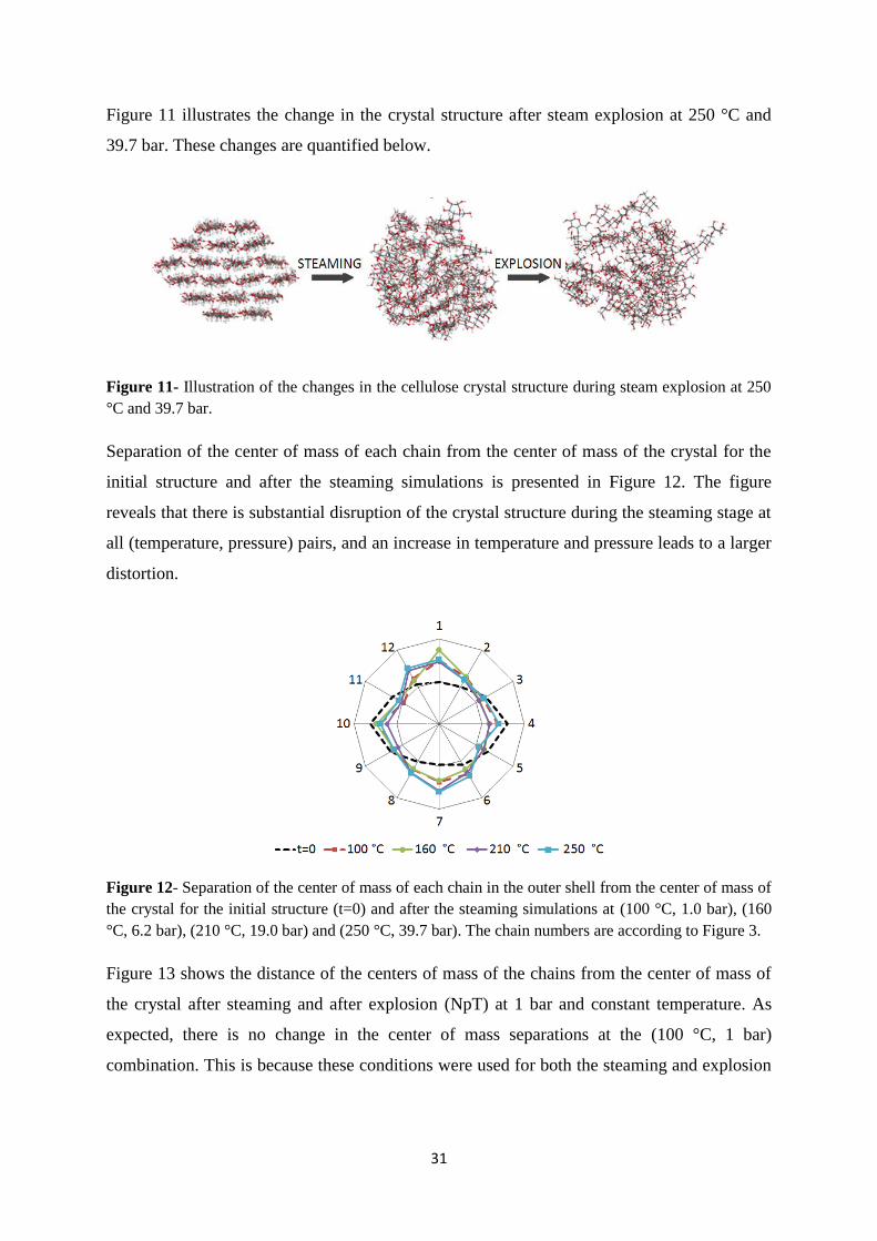
Figure 11 illustrates the change in the crystal structure after steam explosion at 250 °C and

39.7 bar. These changes are quantified below.

Figure 11- Illustration of the changes in the cellulose crystal structure during steam explosion at 250

°C and 39.7 bar.

Separation of the center of mass of each chain from the center of mass of the crystal for the

initial structure and after the steaming simulations is presented in Figure 12. The figure

reveals that there is substantial disruption of the crystal structure during the steaming stage at

all (temperature, pressure) pairs, and an increase in temperature and pressure leads to a larger

distortion.

Figure 12- Separation of the center of mass of each chain in the outer shell from the center of mass of

the crystal for the initial structure (t=0) and after the steaming simulations at (100 °C, 1.0 bar), (160

°C, 6.2 bar), (210 °C, 19.0 bar) and (250 °C, 39.7 bar). The chain numbers are according to Figure 3.

Figure 13 shows the distance of the centers of mass of the chains from the center of mass of

the crystal after steaming and after explosion (NpT) at 1 bar and constant temperature. As

expected, there is no change in the center of mass separations at the (100 °C, 1 bar)

combination. This is because these conditions were used for both the steaming and explosion

32

simulations. The results are included here since they confirm that the system has equilibrated

during steaming and there are therefore no further changes during the subsequent simulation.

Figure 13- Separation of the centres of mass of outer shell chains from the centre of mass of the

crystal after steaming (red dashed line) and after explosion at 1 bar and constant temperature (solid

blue line). The four panels show results at different temperatures.

Similar to the change in the crystal structure during steaming, an increase in temperature and

pressure leads to a larger disruption of the cellulose crystal structure during explosion. Also,

although not shown in the figure (for the sake of clarity), the change in center of mass

separation is largest for the chains in the outer shell compared to those in the core region.

That is, the central cellulose chains (13-18) show very small changes compared to many of

the chains in the outer shell (1-12). For example, the absolute value of the change in centers

of mass of chains 1-12 during the explosion stage at (250 °C, 39.7 bar) is, on average, 1.9 Å,

whereas for the chains in the core it is 0.8 Å.

33

Figure 14 shows the same results as those discussed with reference to Figures 13, but where

the explosion simulations, starting with one of the structures obtained from steaming at (250

°C, 39.7 bar), are performed using NVE molecular dynamics with a volume 26 times larger

than that used for steaming.

Figure 14- Same as Figure 13 but using NVE with the large box to simulate the explosion stage.

The figure shows that there is very little change in the centers of mass of the chains when

performing the explosion simulations under constant energy conditions. Hence, it is the

constant temperature, and not the drop in pressure, that caused the change in centers of mass

during the NpT simulations. Since experimental explosion is performed under NVE

conditions (but where the final pressure is 1 bar), the results obtained here indicate that most

of the disruption of the crystal structure occurs during the steaming stage.

The change in radius of gyration for each chain as a function of its change in center of mass

during explosion at 250 °C and 1 bar is shown in Figure 15. The results are typical for all

initial structures and (temperature, pressure) pairs.

34

Figure 15- Change in radius of gyration for each chain as a function of its change in centre of mass

during explosion at 250 °C and 1 bar. The lines are best-fit straight lines to the core chains (dashed

line), the chains in the outer shell (thin solid line) and all eighteen chains (thick solid line).

Although all three curves show a trend of decreasing change in radius of gyration with

increasing change in centre of mass, there is a large scattering (the R-squared values are 0.42,

0.24 and 0.27 for each of the fits, respectively). This means that there is no statistically

relevant correlation between the change in radius of gyration of each chain and its change in

centre of mass.

The change in separation between the non-reducing end of a chain in the outer shell and the

same end of the neighbouring core chain is shown in Figure 16.

Figure 16- Change in the separation of centre of mass of the non-reducing end (non-Red.), the O-link

in the centre of each chain and reducing end (Red.), between the outer chains and their neighbouring

inner chains. The results are for steaming (red) and NpT explosion (blue) at 250 °C.

The figure reveals that there is larger disruption at the ends of the chains than at the middle

during both steaming and explosion. It should also be noted that the values in the figure are

-1

0

1

2

3

non-Red. O-link Red.

Cha

nge

in s

epar

atio

n (Å

)

Steaming Steaming+Explosion

35

averages over all outer chains, and that some chain ends are separated by as much as 16.1 Å

from the neighboring inner chain ends. Hence, after steaming and explosion the ends of the

crystalline elementary fibrils are more accessible to enzymatic attack than other regions of

the fibril.

At the beginning of the simulations all torsion angles in the chains in the crystal structure are

syn. There was significant change from syn to anti conformation during the steaming and

NpT explosion simulations. For example, after steaming at (250 °C, 39.7 bar) ~15.7% and

~9.9% of the torsions in the chains in the outer shell and core chains were anti, respectively.

The corresponding numbers at (160 °C, 6.2 bar) were ~17.1% and ~7.4%. Explosion at 250

°C resulted in a further increase to ~21.4% for chains in the outer shell and ~14.4% in the

core chains, whereas NpT explosion at 160 °C did not lead to a large increase in the percent

of anti torsions (~17.9% for chains in the outer shell and ~9.1% in the core chains). These

trends are typical for all structures and temperatures, and show that the chains in the outer

shell, which also showed the largest change in center of mass motion, change more readily to

anti torsions than the confined chains in the core region. In addition, a larger percentage of

torsions change to the anti conformer at the higher temperatures and pressures and there is no

significant correlation between the changes in percent anti conformer in a chain with its

change in center of mass.

3.3 Paper IV

Computational studies of water and carbon dioxide interactions with a pair of cellobiose

molecules was performed using the B3LYP/6-311++G** and Grimme’s dispersion

correction. This study yields information on cellobiose-cellobiose bonding mechanisms and

interactions between an H2O or CO2 with the cellobiose pair that can give a deeper

understanding of the steam and SC-CO2 explosion mechanisms.

The goal of this study is to determine if the CO2 molecule yields significantly different low

energy structures compared to when the H2O interacts with the cellobiose pair and to

investigate the relative importance of the inter-cellobiose hydrogen and van der Waals

bonding and how this may differ between the H2O and CO2 complexes.

36

3.3.1 H2O-cellobiose pair

Figure 17 shows the relative energies, ΔE, of the 90 unique H2O-cellobiose pair local

minimum energy structures, ordered according to relative energies obtained from the DFT

with dispersion correction (DFT-D) calculations. These structures were initially geometry

optimized with the COMPASS force field. The energies are relative to the DFT-D energy of

the lowest energy structure. The lowest energy structure obtained from DFT-D also has the

lowest DFT energy (i.e., when dispersion corrections are not included).

Figure 17- Relative energies (in kcal/mol) of local minimum H2O-cellobiose pair structures obtained

from DFT-D and DFT.

The Figure 17 shows that the energy difference between the high and low energy structures is

~25 kcal/mol within the DFT-D series and ~15 kcal/mol within the DFT series. This

difference between the change in DFT-D and DFT energies is due to the extra stability that

the dispersion contributes to the low energy structures. The dispersion correction yields DFT

energies that are ~50 kcal/mol lower in energy than the DFT results.

Structures that have low energy consist of cellobiose molecules that are parallel to each other

and where the glucose units on one of the molecules lie directly above the glucose units on

the second molecule. This maximises the number of hydrogen bonds (which is between 5 and

7 in the low energy structures) and the van der Waals energy. Structures with intermediate

energies consist of cellobiose molecules that lie parallel to each other, but the cellobiose

molecules are shifted relative to each other that result in fewer hydrogen bonds (3-5) and

reduced van der Waals attraction. In the structures with the highest energies, the cellobiose

molecules have almost no overlap of the glucose units. There are only 1 or 2 hydrogen bonds

and the van der Waals interactions are far weaker.

37

Figure 18- Lowest energy H2O-cellobiose pair structure obtained from DFT-D. The H2O molecule is

shown in blue.

Figure 18 shows the lowest energy structure obtained from DFT-D. There are six hydrogen

bonds in this structure that are between O3--H-O2´, O6--H-O6´, H-O4--O1´, O4--H-O1´,

O1´-H--O3 and O6´-H--O6, where the first number in each bond is for Cellob.1 and the

second for Cellob.2. The H2O molecule is attached to the cellobiose pair by two hydrogen

bonds in the minimum energy structure. The distance between centre of masses of the H2O

and Cellob.2 is 5.63 Å. The intermolecular energy between the H2O and the cellobiose pair is

-15.5 kcal/mol.

Table 3- Cellobiose-cellobiose intermolecular energies (Einter-pair) and the dispersion correction

energies (Edisp) in kcal/mol for some structures shown in Figure 17.

Structure No. Einter-pair Edisp (%)

1 -51.5 -17.8 (35)

6 -46.8 -18.5 (40)

14 -51.2 -17.6 (34)

37 -42.2 -20.8 (49)

40 -27.4 -11.2 (41)

46 -38.2 -14.6 (38)

48 -33.0 -20.3 (62)

78 -34.6 -16.7 (48)

82 -29.4 -18.6 (63)

86 -12.6 -9.7 (77)

88 -13.8 -4.4 (32)

90 -17.3 -6.3 (36)

Table 3 represents DFT-D intermolecular energies (Einter-pair) and the dispersion correction

energies (Edisp) of cellobiose-cellobiose pairs in kcal/mol for some structures of Figure 17. It

is evident that the intermolecular energy decreases with increasing structure number i.e. when

relative energy increases. The dispersion contributions to the inter-cellobiose energies and the

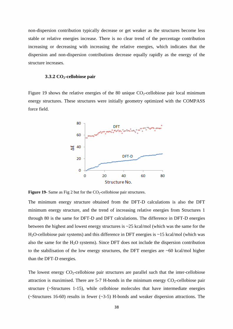
38

non-dispersion contribution typically decrease or get weaker as the structures become less

stable or relative energies increase. There is no clear trend of the percentage contribution

increasing or decreasing with increasing the relative energies, which indicates that the

dispersion and non-dispersion contributions decrease equally rapidly as the energy of the

structure increases.

3.3.2 CO2-cellobiose pair

Figure 19 shows the relative energies of the 80 unique CO2-cellobiose pair local minimum

energy structures. These structures were initially geometry optimized with the COMPASS

force field.

Figure 19- Same as Fig 2 but for the CO2-cellobiose pair structures.

The minimum energy structure obtained from the DFT-D calculations is also the DFT

minimum energy structure, and the trend of increasing relative energies from Structures 1

through 80 is the same for DFT-D and DFT calculations. The difference in DFT-D energies

between the highest and lowest energy structures is ~25 kcal/mol (which was the same for the

H2O-cellobiose pair systems) and this difference in DFT energies is ~15 kcal/mol (which was

also the same for the H2O systems). Since DFT does not include the dispersion contribution

to the stabilisation of the low energy structures, the DFT energies are ~60 kcal/mol higher

than the DFT-D energies.

The lowest energy CO2-cellobiose pair structures are parallel such that the inter-cellobiose

attraction is maximised. There are 5-7 H-bonds in the minimum energy CO2-cellobiose pair

structure (~Structures 1-15), while cellobiose molecules that have intermediate energies

(~Structures 16-60) results in fewer (~3-5) H-bonds and weaker dispersion attractions. The

39

structures with the highest relative energies (~Structures 61-80) have even fewer H-bonds

and weaker van der Waals attraction.

Figure 20 is the minimum energy CO2-cellobiose pair structure. The separation between the

cellobiose centres of mass is 4.10 Å. Both cellobiose molecules have the anti conformation,

with φH = 177.5 and 177.0° for Cellob.1 and Cellob.2, respectively. There are seven H-bonds,

which are located between O6--H-O3´, O3´--H-O6, O3-H--O3, O2´-H--O6, O3´-H--O6´,

O4´-H--O5´ and O6´-H--O4´, where the first number in each bond refers to the Cellob.1

molecule and the second number to Cellob.2.

Figure 20- CO2-cellobiose pair minimum energy structure. The CO2 molecule is shown in brown.

The distance between the centre of mass of the CO2 molecule and the cellobiose pair in the

minimum energy structure shown in Figure 20 is 7.51 Å. Neither this distance, nor the CO2-

cellobiose intermolecular energy, shows a systematic change with increasing structure

number. For example, this energy is -8.2, -9.4 and -5.6 kcal/mol for Structures 1, 21 and 72,

respectively.

Table 4 shows that the inter-cellobiose energy decreases by increasing relative energy. The

dispersion energy and the non-dispersion contribution to the intermolecular energy also

decrease. Similarly to the H2O-cellobiose pair systems, there is no clear evidence that the

relative contribution of the dispersion energy (shown as percent in parenthesis in the table)

either increases or decreases with increasing structure number.

40

Table 4- same as Table 3, but for CO2-cellobiose pair systems

Structure No. Einter-pair Edisp (%)

1 -56.6 -23.3 (41)

3 -54.9 -22.4 (41)

11 -46.7 -19.1 (41)

19 -38.0 -20.7 (54)

21 -34.0 -13.4 (39)

22 -25.6 -17.8 (70)

28 -30.2 -20.0 (66)

34 -29.4 -19.2 (65)

46 -23.6 -12.2 (52)

54 -18.9 -6.0 (32)

65 -12.9 -11.2 (87)

72 -17.4 -6.1 (35)

3.4 Paper V

The relative energies obtained from DFT-D, DFT and the COMPASS force field for CO2- cellobiose

pair systems are shown in Figure 21. The numbering of the structures is according to the lowest

energy structure obtained from DFT-D method. DFT energies are obtained from the DFT-D

optimisations and where the dispersion corrections have not been added to the total energy.

Figure 21- Relative energies of local minimum CO2-cellobiose pair structures obtained from DFT-D,

DFT and the COMPASS force field.

Figure 21 shows that the total energies obtained from DFT-D, DFT and COMPASS follow

the same trends, such that the low and high energy structures obtained from DFT and the

COMPASS force field are typically the same as the structures obtained from DFT-D. The

0

5

10

15

20

25

30

0 20 40 60 80

∆E(

kcal

/mo

l)

Structure No.

DFT-D DFT COMPASS

41

lowest energy structure that is obtained from DFT-D (first structure) has a COMPASS

relative energy of 1.1 kcal/mol. All of these low energy structures are similar in geometry and

are more compact compared to the higher energy structures. Hence, the COMPASS force

field correctly describes the trends of compact structures having lower relative energies than

structures where the cellobiose units have shifted relative to each other.

The lowest energy CO2-cellobiose pair structure obtained from DFT-D (right) and the initial

structure obtained from geometry optimisation using the COMPASS force field (left) are

shown in Figure 22.

Figure 22- Lowest energy CO2-cellobiose pair structure obtained from DFT-D. The initial structure

obtained from geometry optimisation using the COMPASS force field is shown on the left and that

obtained from the DFT-D optimization is shown on the right.

It is evident that these structures are similar; hence, geometry optimisation with DFT-D only

leads to small changes in the structure obtained from the COMPASS force field. For instance,

the separation between the cellobiose centres of mass is 3.85 Å in the structure obtained from

the COMPASS force field and it is 4.10 Å according to DFT-D (more details can be found in

Paper V). In both structures, seven H-bonds are formed by the same atoms. Both methods

yield cellobiose molecules with the anti conformation. These similarities indicate that the

COMPASS force field provides a valid description for the trends of CO2 interacting with

cellulose and for the disruption of the cellulose crystal structure. It was therefore used to

study these trends during SC-CO2 explosion of cellulose.

Similarly to the steam explosion, the molecular-level studies of dissolution of the crystalline

structure of cellulose were simulated using grand canonical Monte Carlo and molecular

dynamics. The SC-CO2 explosion was at different temperature/ pressure combinations of 110

°C/ 2500 psi, 110 °C/ 3000 psi, 110 °C/3500, 110 °C/ 4000 psi, 135 °C/ 3500 psi, 165 °C/

3500 psi and 200 °C/ 3500 psi.

42

Figure 23 illustrates the change in the crystal structure after steam explosion at 250 °C and

39.7 bar. These changes are quantified below.

Figure 23- Illustration of the changes in the cellulose crystal structure during SC-CO2 explosion at

200 °C and 3500 psi.

The changes in the centres of mass for each chain relative to the centre of mass of the crystal

are shown in Figure 24.

Figure 24- Centre of mass of each chain 1-18 relative to the centre of mass of the crystal for the

initial structure (t0) and after loading and explosion. Results are for Systems (110 °C/ 2500 psi), (110

°C/ 3500 psi) and (200 °C/ 3500) and the standard deviations are from the three trajectories

43

propagated at each temperature/ pressure combination. The standard deviations are shown as error

bars.

Figure 24 shows that during SC-CO2 loading and explosion the centres of mass of chains 3-5,

9-11, 15 and 18 decrease while other chains show an increase in centres of mass relative to

the centre of mass of the crystal. This occurs since the pressure of the SC-CO2 makes the

cross section of the crystal structure more circular. The figure also shows that displacement

of the chains in the outer layer (chains 1-12) is larger than chains in the core and changes in

the chains in the outer shell affect the displacement of their neighbouring chains in the core.

For example, during loading, chains 1 and 7 move away from the centre of the crystal by

about 4.3 and 3.9 Å, while chains 4 and 10 move closer to the centre about 2.7 and 2.1 Å.

Similarly, chains 13 and 16, which neighbour chains 1 and 7, respectively, move out by about

1.1 and 2.9 Å, respectively, while chains 15 and 18 move inwards by about 0.7 Å. As shown

in Figure 22, most of the changes occur during loading of the SC-CO2, and explosion has a

far smaller effect on the disruption of the structure.

The effect of temperature and pressure on SC-CO2 loading and explosion was studied using

two sets of chains. The first set was chains 1, 6, 7 and 12 and the second set was chains 4, 5,

10 and 11. These sets were chosen since the chains are all in the outer shell and the chains in

the first set increase their centre of mass during loading and explosion and the chains in the

second set decreases their centre of mass.

3.4.1 Effect of temperature

The left panel in Figure 25 shows the effect of increasing temperature on the average change

in centre of mass of chains 1, 6, 7 and 12 after loading and the combined loading and

explosion. The pressure is 3500 psi and the temperature increases from 110 to 200 °C. The

right panel is the same but for chains 4, 5, 10 and 11.

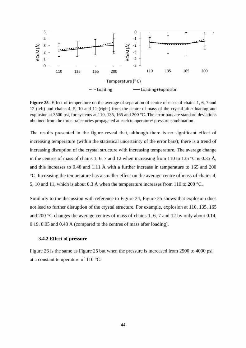
44

Figure 25- Effect of temperature on the average of separation of centre of mass of chains 1, 6, 7 and

12 (left) and chains 4, 5, 10 and 11 (right) from the centre of mass of the crystal after loading and

explosion at 3500 psi, for systems at 110, 135, 165 and 200 °C. The error bars are standard deviations

obtained from the three trajectories propagated at each temperature/ pressure combination.

The results presented in the figure reveal that, although there is no significant effect of

increasing temperature (within the statistical uncertainty of the error bars); there is a trend of

increasing disruption of the crystal structure with increasing temperature. The average change

in the centres of mass of chains 1, 6, 7 and 12 when increasing from 110 to 135 °C is 0.35 Å,

and this increases to 0.48 and 1.11 Å with a further increase in temperature to 165 and 200

°C. Increasing the temperature has a smaller effect on the average centre of mass of chains 4,

5, 10 and 11, which is about 0.3 Å when the temperature increases from 110 to 200 °C.

Similarly to the discussion with reference to Figure 24, Figure 25 shows that explosion does

not lead to further disruption of the crystal structure. For example, explosion at 110, 135, 165

and 200 °C changes the average centres of mass of chains 1, 6, 7 and 12 by only about 0.14,

0.19, 0.05 and 0.48 Å (compared to the centres of mass after loading).

3.4.2 Effect of pressure

Figure 26 is the same as Figure 25 but when the pressure is increased from 2500 to 4000 psi

at a constant temperature of 110 °C.

0

1

2

3

4

5

110 135 165 200

Load Load+Expl.

∆C

oM

(Å)

Temperature ( ° C)

-5

-4

-3

-2

-1

0

110 135 165 200

Load Laod+ Expl.

Temperature ( ° C)

∆C

oM

(Å)

0

0.5

1

1.5

2

2.5

3

3.5

4

4.5

5

(C) 110 (E) 135 (F) 165 (G) 200

Loading Loading+Explosion

∆C

oM

(Å)

Temperature (° C)

45

Figure 26- Same as for Figure 25 but for systems 2500, 3000, 3500 and 4000 psi. The temperature is

110 °C for all systems.

There is a larger change in separation of the centre of mass of the chains relative to the

centre of the crystal at lower pressures. This is probably due to the fact that lower pressures

allow chains 1, 6, 7 and 12 to move further away from the centre of the crystal than at higher

pressures. This, in turn, means that chains 4, 5, 7 and 10 can move towards the centre of the

crystal at the lower pressures. For example, increasing the pressure from 2500 to 3000 psi

decreases the average change in centre of mass separation for chains 1, 6, 7 and 12 by 0.48 Å

during loading. Further increases in pressure to 3500 and 4000 psi leads to larger decreases

of 0.78 and 1.27 Å compared to 2500 psi. Similarly, the average change in centre of mass

separation for chains 4, 5, 7 and 10 differs by 0.8 Å between pressures of 2500 and 3000 psi,

1.1 Å between 2500 and 3500 psi and 1.8 Å between 2500 and 4000 psi.

Figure 27- Change in the separation of centre of mass of the non-reducing end (non-Red.), the O-link

in the centre of each chain and reducing end (Red.) between the outer chains and their neighbouring

-4

-3

-2

-1

0

1

2500 3000 3500 4000

∆C

oM

(Å)

0

1

2

3

4

5

2500 3000 3500 4000

∆C

oM

(Å)

-4-3-2-101

2500 3000 3500 4000

Loading Loading+ Explosion

Pressure (psi)∆

Co

M(Å

)

-1

0

1

2

no

n-R

ed

.

O-l

ink

Re

d.

no

n-R

ed

.

O-l

ink

Re

d.

no

n-R

ed

.

O-l

ink

Re

d.

110 °C, 3500 psi (C)

110 °C, 4000 psi (D)

200 °C, 3500 psi (G)

Ch

an

ge

in s

ep

ara

tio

n (

Å)

Loading Loading+ Explosion

46

inner chains during loading and explosion. The results are shown for loading and explosion at 110 °C

and 3500 psi, 110 °C and 4000 psi and 200 °C and 3500 psi.

Figure 27 reveals that there is a larger disruption at the ends of the chains than in the middle

(O-link) during both loading and explosion. Hence, there is larger disruption at the ends of

the crystal structure (i.e., at the chain ends) than in the middle of the crystal. This would lead

to enhanced accessibility for enzymatic hydrolysis at the crystal ends rather than in the

middle of the crystal.

No significant correlation was observed between the magnitude of the change in centres of

mass of chains during loading and explosion with changes in their radii of gyration.

47

4 Conclusions and Outlook

The COMPASS force field was preferred over the Dreiding and Universal force fields for

study of glucose and cellobiose molecules as well as cellulose structural changes during

dissolution with steam and supercritical carbon dioxide (SC-CO2).

The validity of the COMPASS force field was checked by comparing the resulted structures

and energies from first principles calculations and force field methods for glucose and

cellobiose. These molecular systems were selected since they are sufficiently small to

perform the first principles calculations in a tractable time and also being relevant to the

dissolution of cellulose in water. The comparison was also made with relative energies and

structures calculated by others using the B3LYP/6-311++G** method. The COMPASS force

field was the only force field that yields the correct anti conformer of cellobiose and gave the

minimum energy structure in vacuum and syn conformer in vacuum at high temperature and

in aqueous environment at 1 bar and 298 K. The COMPASS force field also indicates that the

crystal structure of cellulose has lower energy than the separated cellulose chains.

According to previous studies, the B3LYP/6-311++G** density functional method yields

valid energies and structures for cellobiose and H2O-cellobiose systems. This method,

including Grimme’s dispersion correction, was used to study the interactions between several

structures containing H2O or CO2 and two cellobiose molecules that were initially optimized

using the COMPASS force field.

Comparison of the intermolecular energies of cellobiose-cellobiose obtained from DFT and

DFT-D showed that both the non-dispersion and dispersion terms have large contributions

(between 30 and 70 %.) to the intermolecular energies.

Geometry optimisation with the DFT-D method showed that the H2O and CO2 molecules

prefer to bond to the surface of the cellobiose pair and opposed to being located between the

cellobiose molecules.

The intermolecular energies obtained from DFT-D calculations also showed that when a H2O

molecule interacts with two cellobiose molecules, the intermolecular interactions between the

two cellobiose molecules are weaker than when a CO2 molecule interacts with the cellobiose

48

molecules. This is due to larger electron density that is located between the cellobiose pair

and the water molecule.

Studies of steam and supercritical carbon dioxide (SC-CO2) explosion were performed using

grand canonical Monte Carlo and molecular dynamics based on the COMPASS force field.

The calculations are based on the crystalline structure of cellulose that was proposed by Ding

and Himmel. In these studies restructuring of the cellulose crystal were investigated by

changes in the centres of mass of cellulose chains during loading of saturated steam

(steaming) and SC-CO2 and explosion steps. For both solvents disruption was larger for the

chains in the outer shell compared to the core chains and comparison between chains within

either the outer shell or core region showed that there was no significant correlation between

changes in the radius of gyration and the change in centre of mass of the chains. Also, for

both methods increasing the temperature leads to more disruption in the cellulose crystal.

During SC-CO2 explosion, increasing the pressure decreases the disruption of the crystal.

Comparing the centre of mass of neighbour chains, larger distortion of the crystal structure

was seen at the ends of the crystal. Increase in disruption of the cellulose crystals due to

increasing temperature, enhances accessibility of enzymes to the cellulose chains which

particularly happens at the ends of the elementary fibrils and is important for the cellulose

pretreatment in production of biofuel.

49

Future work

Several pretreatment processes have been developed for decreasing the recalcitrance and

increasing dissolution of cellulose in several solvents, but only a few of them seem to be

promising. N-methyl morpholine-N-oxide (NMMO) hydrate is an effective and direct solvent

for dissolution of cellulose. Different proportion of water has different effects on the

dissolution of cellulose. For example NMMO–water mixture containing 83% and 87% (w/w)

NMMO (monohydrate) is known as dissolution mode and the cellulose fibres can be dissolve

completely, while in a mixture with 76–82% NMMO, cellulose dissolves partially in the

produced fibre balloons. Lower NMMO contents of 70–75% cause partial ballooning and

swelling. Less NMMO content shows no effect on dissolution of cellulose fibres [99, 100].

The studies presented here, can be applied for molecular-level investigation of the dissolution

of cellulose with different NMMO-water percentage.

The studies presented in this thesis shows the effect of steam and SC-CO2 explosion on an 18

chains elementary fibril, the study can be extended to the 36 chains model and to microfibrils

containing several elementary fibrils.

There is also no molecular-level study of the pretreatment for other proposed models of

cellulose structures; these studies can also be executed on the different models of cellulose

elementary and microfibrils.

50

Acknowledgements

First, I would like to express my deep gratitude to my supervisor Prof. Kim Bolton for

accepting me as a student and for his patient guidance, enthusiastic encouragement and useful

critiques of this research work.

My grateful thanks are also extended to my examiner Prof. Claes Niklasson and my co-

supervisor Assoc. Prof. Peter Ahlström.

I would also like to thank Prof. Frank Momany for his great and helpful contribution in my

first paper and Prof. Mohammad Taherzadeh for his assistance.

I am very thankful to my colleagues in modelling group: Anders, Edvin, Kavitha, Martin,

Shayesteh and Abas for their good collaboration.

I would like to express my appreciation to all staffs at the School of Engineering,

University of Borås for providing such a friendly environment. Peter, Ilona, Thomas S.,

Solveg, Louise and Sari are gratefully acknowledged for their helps.

My sincere thank also goes to Martin Bohlén for being such a good colleague.

I wish also to thanks my friends and all former and present PhD students at the University of

Borås especially Behnaz, Azadeh, Shayesteh, Supansa, Päivi, Farzad, Abas, Tariq, Kamran

and Mofoluwake.

I am grateful to Stiftelsen Foreningssparbanken Sjuharad and the Carl Trygger Foundation

for Scientific Research for the financial support. The Quantum Mechanics calculations were

performed on resources provided by the Swedish National Infrastructure for Computing

(SNIC) at NSC, HPC2N and C3SE. Molecular Mechanics results were obtained using

program from Accelrys Software Inc.

My special thanks to my parents, Zahra and Heidar for their endless love, supports and

encouragements. I wish also to thanks my lovely sisters, Parisa and Bita.

Thanks with love to my kind husband, Mehdi for his support, love, patience and

encouragements.

And finally my greatest thanks to my wonderful children, Sahand and Soren for their patience

and understanding.

51

References

1. Goldemberg, J. (2007). Ethanol for a sustainable energy future. science,315(5813),

808-810.

2. Orfao, J. J. M., Antunes, F. J. A., & Figueiredo, J. L. (1999). Pyrolysis kinetics of

lignocellulosic materials—three independent reactions model. Fuel, 78(3), 349-358.

3. Lucia, L. A. (2008). Lignocellulosic biomass: A potential feedstock to replace

petroleum. BioResources, 3(4), 981-982.

4. Limayem, A., & Ricke, S. C. (2012). Lignocellulosic biomass for bioethanol

production: current perspectives, potential issues and future prospects.Progress in

Energy and Combustion Science, 38(4), 449-467.

5. Ho, M. W. (2006). Ethanol from cellulose biomass not sustainable nor

environmentally benign. Science in Society, (30), 32-35.

6. Taherzadeh, M. J., & Karimi, K. (2007). Enzymatic-based hydrolysis processes for

Ethanol. BioResources, 2(4), 707-738.

7. Jin, Z., Katsumata, K. S., Lam, T. B. T., & Iiyama, K. (2006). Covalent linkages

between cellulose and lignin in cell walls of coniferous and nonconiferous

woods. Biopolymers, 83(2), 103-110.

8. Festucci-Buselli, R. A., Otoni, W. C., & Joshi, C. P. (2007). Structure, organization,

and functions of cellulose synthase complexes in higher plants.Brazilian Journal of

Plant Physiology, 19(1), 1-13.

9. Esteghlalian, A., Hashimoto, A. G., Fenske, J. J., & Penner, M. H. (1997). Modeling

and optimization of the dilute-sulfuric-acid pretreatment of corn stover, poplar and

switchgrass. Bioresource Technology, 59(2), 129-136.

10. Davin, L. B., Patten, A. M., Jourdes, M., & Lewis, N. G. (2008). Lignins: a

twenty‐first century challenge. Biomass Recalcitrance: Deconstructing the Plant Cell

Wall for Bioenergy, 213-305.

11. Mudhoo, A. (Ed.). (2012). Biogas production: pretreatment methods in anaerobic

digestion. John Wiley & Sons.

12. Pethrick, R. A. (Ed.). (2007). Polymer structure characterization: from nano to macro

organization. Royal Society of Chemistry.

13. Pérez, J., Munoz-Dorado, J., de la Rubia, T. D. L. R., & Martinez, J. (2002).

Biodegradation and biological treatments of cellulose, hemicellulose and lignin: an

overview. International Microbiology, 5(2), 53-63.

14. Fengel, D., & Wegener, G. (Eds.). (1983). Wood: chemistry, ultrastructure, reactions.

Walter de Gruyter.

15. Zugenmaier, P. (2008). Cellulose (pp. 101-174). Springer Berlin Heidelberg.

52

16. Ding, S. Y., & Himmel, M. E. (2006). The maize primary cell wall microfibril: a new

model derived from direct visualization. Journal of Agricultural and Food

Chemistry, 54(3), 597-606.

17. Stone, B. (2005). Cellulose: Structure and distribution. eLS.

18. O'SULLIVAN, A. C. (1997). Cellulose: the structure slowly unravels. Cellulose,4(3),

173-207.

19. Newman, R. H., Ha, M. A., & Melton, L. D. (1994). Solid-state 13C NMR

investigation of molecular ordering in the cellulose of apple cell walls. Journal of

agricultural and food chemistry, 42(7), 1402-1406.

20. Newman, R. H., Davies, L. M., & Harris, P. J. (1996). Solid-state 13C nuclear

magnetic resonance characterization of cellulose in the cell walls of Arabidopsis

thaliana leaves. Plant physiology, 111(2), 475-485.

21. Smith, B. G., Harris, P. J., Melton, L. D., & Newman, R. H. (1998). Crystalline

cellulose in hydrated primary cell walls of three monocotyledons and one

dicotyledon. Plant and cell physiology, 39(7), 711-720.

22. Himmel, M. E. (2009). Biomass recalcitrance: deconstructing the plant cell wall for

bioenergy. Wiley-Blackwell.

23. Strati, G. L., Willett, J. L., & Momany, F. A. (2002). Ab initio computational study of

β-cellobiose conformers using B3LYP/6-311++ G**. Carbohydrate

research, 337(20), 1833-1849.

24. Bazooyar F., B.M., Bolton K., Computational Studies of Water and Carbon Dioxide

Interactions with Cellobiose. Journal of Molecular Modeling, 2014. Submitted.

25. Bosma, W. B., Appell, M., Willett, J. L., & Momany, F. A. (2006). Stepwise

hydration of cellobiose by DFT methods: 1. Conformational and structural changes

brought about by the addition of one to four water molecules. Journal of Molecular

Structure: THEOCHEM, 776(1), 1-19.

26. Taherzadeh, M. J., & Karimi, K. (2008). Pretreatment of lignocellulosic wastes to

improve ethanol and biogas production: a review. International journal of molecular

sciences, 9(9), 1621-1651.

27. Silverstein, R. A. (2005). A comparison of chemical pretreatment methods for

converting cotton stalks to ethanol.

28. Johnson, D. K., & Elander, R. T. (2008). Pretreatments for enhanced digestibility of

feedstocks. Biomass recalcitrance: Deconstructing the plant cell wall for bioenergy,

436-453.

29. Kumar, P., Barrett, D. M., Delwiche, M. J., & Stroeve, P. (2009). Methods for

pretreatment of lignocellulosic biomass for efficient hydrolysis and biofuel

production. Industrial & Engineering Chemistry Research, 48(8), 3713-3729.

53

30. Mason, W. H. (1926). U.S. Patent No. 1,578,609. Washington, DC: U.S. Patent and

Trademark Office.

31. BABCOCK, L. W. (1932). U.S. Patent No. 1,855,464. Washington, DC: U.S. Patent

and Trademark Office.

32. Volynets, B., & Dahman, Y. (2011). Assessment of pretreatments and enzymatic

hydrolysis of wheat straw as a sugar source for bioprocess industry.Int J Energy

Environ, 2(3), 427-446.

33. Josefsson, T., Lennholm, H., & Gellerstedt, G. (2002). Steam explosion of aspen

wood. Characterisation of reaction products. Holzforschung, 56(3), 289-297.

34. Ballesteros, I., Negro, M. J., Oliva, J. M., Cabañas, A., Manzanares, P., & Ballesteros,

M. (2006, January). Ethanol production from steam-explosion pretreated wheat straw.

In Twenty-Seventh Symposium on Biotechnology for Fuels and Chemicals (pp. 496-

508). Humana Press.

35. Schultz, T. P., Biermann, C. J., & McGinnis, G. D. (1983). Steam explosion of mixed

hardwood chips as a biomass pretreatment. Industrial & Engineering Chemistry

Product Research and Development, 22(2), 344-348.

36. Gao, M., Xu, F., Li, S., Ji, X., Chen, S., & Zhang, D. (2010). Effect of SC-CO2

pretreatment in increasing rice straw biomass conversion.Biosystems

engineering, 106(4), 470-475.

37. Donaldson, L. A., Wong, K. K. Y., & Mackie, K. L. (1988). Ultrastructure of steam-

exploded wood. Wood science and technology, 22(2), 103-114.

38. Martin-Sampedro, R., Capanema, E. A., Hoeger, I., Villar, J. C., & Rojas, O. J.

(2011). Lignin changes after steam explosion and laccase-mediator treatment of

eucalyptus wood chips. Journal of agricultural and food chemistry, 59(16), 8761-

8769.

39. Jedvert, K., Saltberg, A., Lindström, M., & Theliander, H. (2011). Extraction of

hemicelluloses after chemical pretreatment combined with mild steam explosion.

In 16th International Symposium on Wood, Fiber and Pulping Chemistry, ISWFPC,

Tianjin, 8 June through 10 June 2011 (Vol. 2, pp. 867-871).

40. Chacha, N., Toven, K., Mtui, G., Katima, J., & Mrema, G. (2011). Steam pretreatment

of pine (Pinus patula) wood residue for the production of reducing sugars. Cellulose

Chemistry and Technology, 45(7), 495.

41. Eckert, C. A. (1996). Supercritical fluids as solvents for chemical and materials

processing. Nature, 383, 313-318.

42. Zheng, Y., Lin, H. M., Wen, J., Cao, N., Yu, X., & Tsao, G. T. (1995). Supercritical

carbon dioxide explosion as a pretreatment for cellulose hydrolysis. Biotechnology

Letters, 17(8), 845-850.

54

43. Paljevac, M., Primožič, M., Habulin, M., Novak, Z., & Knez, Ž. (2007). Hydrolysis of

carboxymethyl cellulose catalyzed by cellulase immobilized on silica gels at low and

high pressures. The Journal of Supercritical Fluids, 43(1), 74-80.

44. Canelas, D. A., & DeSimone, J. M. (1997). Polymerizations in liquid and supercritical

carbon dioxide. In Metal Complex Catalysts Supercritical Fluid Polymerization

Supramolecular Architecture (pp. 103-140). Springer Berlin Heidelberg.

45. Alinia, R., Zabihi, S., Esmaeilzadeh, F., & Kalajahi, J. F. (2010). Pretreatment of

wheat straw by supercritical CO2 and its enzymatic hydrolysis for sugar

production. Biosystems engineering, 107(1), 61-66.

46. Alvira, P., Tomás-Pejó, E., Ballesteros, M., & Negro, M. J. (2010). Pretreatment

technologies for an efficient bioethanol production process based on enzymatic

hydrolysis: a review. Bioresource technology, 101(13), 4851-4861.

47. Koch, W., Holthausen, M. C., & Holthausen, M. C. (2001). A chemist's guide to

density functional theory (Vol. 2). Weinheim: Wiley-Vch.

48. Luterbacher, J. S., Tester, J. W., & Walker, L. P. (2010). High‐solids biphasic CO2–

H2O pretreatment of lignocellulosic biomass. Biotechnology and

bioengineering, 107(3), 451-460.

49. Narayanaswamy, N., Faik, A., Goetz, D. J., & Gu, T. (2011). Supercritical carbon

dioxide pretreatment of corn stover and switchgrass for lignocellulosic ethanol

production. Bioresource technology, 102(13), 6995-7000.

50. Ritter, D. C., & Campbell, A. G. (1991). Supercritical carbon dioxide extraction of

southern pine and ponderosa pine. Wood and Fiber Science, 23(1), 98-113.

51. Zheng, Y., & Tsao, G. T. (1996). Avicel hydrolysis by cellulase enzyme in

supercritical CO2. Biotechnology letters, 18(4), 451-454.

52. Zheng, Y., Lin, H. M., & Tsao, G. T. (1998). Pretreatment for cellulose hydrolysis by

carbon dioxide explosion. Biotechnology progress, 14(6), 890-896.

53. Kim, K. H., & Hong, J. (2001). Supercritical CO2 pretreatment of lignocellulose

enhances enzymatic cellulose hydrolysis. Bioresource Technology, 77(2), 139-144.

54. Hehre, W. J. (2003). A guide to molecular mechanics and quantum chemical

calculations (p. p19). Irvine, CA: Wavefunction.

55. Cramer, C. J., & Bickelhaupt, F. M. (2003). Essentials of computational

chemistry. ANGEWANDTE CHEMIE-INTERNATIONAL EDITION IN ENGLISH-

,42(4), 381-381.

56. Jensen, F. (2007). Introduction to computational chemistry. John Wiley & Sons.

57. Börjesson, A. (2010). In Silico Studies of Carbon Nanotubes and Metal Clusters.

Department of Physics; Institutionen för fysik.

58. Born, M., & Oppenheimer, R. (1927). Zur quantentheorie der molekeln. Annalen der

Physik, 389(20), 457-484.

55

59. Schweber, S. S. (2011). An introduction to relativistic quantum field theory. Courier

Dover Publications.

60. Heisenberg, W. (1974). The uncertainty principle. Educational Materials and

Equipment.

61. Sadlej, A. J. (1991). Medium-size polarized basis sets for high-level-correlated

calculations of molecular electric properties. Theoretica chimica acta, 81(1-2), 45-63.

62. Young, D. (2004). Computational chemistry: a practical guide for applying

techniques to real world problems. John Wiley & Sons.

63. Nesbet, R. K. (1955). Configuration interaction in orbital theories. Proceedings of the

Royal Society of London. Series A. Mathematical and Physical Sciences, 230(1182),

312-321.

64. Møller, C., & Plesset, M. S. (1934). Note on an approximation treatment for many-

electron systems. Physical Review, 46(7), 618.

65. Hinchliffe, A. (2005). Molecular modelling for beginners. John Wiley & Sons.

66. Andrew R. Leach. (2001). Molecular modelling: principles and applications. Pearson

Education.

67. Steinmann, S. N. (2012). Understanding and Minimizing Density Functional Failures

Using Dispersion Corrections (Doctoral dissertation, ÉCOLE POLYTECHNIQUE

FÉDÉRALE DE LAUSANNE).

68. Dirac, P. A. (1930, July). Note on exchange phenomena in the Thomas atom.

InMathematical Proceedings of the Cambridge Philosophical Society (Vol. 26, No.

03, pp. 376-385). Cambridge University Press.

69. Slater, J. C. (1951). A simplification of the Hartree-Fock method. Physical

Review, 81(3), 385.

70. Perdew, J. P., Burke, K., & Wang, Y. (1996). Generalized gradient approximation for

the exchange-correlation hole of a many-electron system.Physical Review B, 54(23),

16533.

71. Perdew, J. P., Chevary, J. A., Vosko, S. H., Jackson, K. A., Pederson, M. R., Singh,

D. J., & Fiolhais, C. (1992). Atoms, molecules, solids, and surfaces: Applications of

the generalized gradient approximation for exchange and correlation. Physical Review

B, 46(11), 6671.

72. Heyd, J., Scuseria, G. E., & Ernzerhof, M. (2003). Hybrid functionals based on a

screened Coulomb potential. The Journal of Chemical Physics, 118(18), 8207-8215.

73. Becke, A. D. (1993). Density‐functional thermochemistry. III. The role of exact

exchange. The Journal of Chemical Physics, 98(7), 5648-5652.

74. Lee, C., Yang, W., & Parr, R. G. (1988). Development of the Colle-Salvetti

correlation-energy formula into a functional of the electron density. Physical Review

B, 37(2), 785.

56

75. Miehlich, B., Savin, A., Stoll, H., & Preuss, H. (1989). Results obtained with the

correlation energy density functionals of Becke and Lee, Yang and Parr.Chemical

Physics Letters, 157(3), 200-206.

76. Stephens, P. J., Devlin, F. J., Chabalowski, C. F., & Frisch, M. J. (1994). Ab initio

calculation of vibrational absorption and circular dichroism spectra using density

functional force fields. The Journal of Physical Chemistry, 98(45), 11623-11627.

77. Cohen, A. J., Mori-Sánchez, P., & Yang, W. (2011). Challenges for density functional

theory. Chemical reviews, 112(1), 289-320.

78. Heyd, J., & Scuseria, G. E. (2004). Efficient hybrid density functional calculations in

solids: assessment of the Heyd–Scuseria–Ernzerhof screened Coulomb hybrid

functional. The Journal of chemical physics, 121(3), 1187-1192.

79. Grimme, S. (2006). Semiempirical GGA‐type density functional constructed with a

long‐range dispersion correction. Journal of computational chemistry,27(15), 1787-

1799.

80. Shattuck, T. W. (2003). Colby College Molecular Mechanics Tutorial QUANTA

Version.

81. Lewars, E. (2010). Computational chemistry: introduction to the theory and

applications of molecular and quantum mechanics. Springer.

82. Moloy, E. C., Davila, L. P., Shackelford, J. F., & Navrotsky, A. (2002). High-silica

zeolites: a relationship between energetics and internal surface areas.Microporous and

mesoporous materials, 54(1), 1-13.

83. Levitt, M., & Lifson, S. (1969). Refinement of protein conformations using a

macromolecular energy minimization procedure. Journal of molecular biology,46(2),

269-279.

84. Fletcher, R., & Reeves, C. M. (1964). Function minimization by conjugate

gradients. The computer journal, 7(2), 149-154.

85. Ermer, O. (1976). Calculation of molecular properties using force fields. Applications

in organic chemistry. In Bonding forces (pp. 161-211). Springer Berlin Heidelberg.

86. Sun, H. (1998). COMPASS: an ab initio force-field optimized for condensed-phase

applications overview with details on alkane and benzene compounds.The Journal of

Physical Chemistry B, 102(38), 7338-7364.

87. Jorgensen, W. L., Maxwell, D. S., & Tirado-Rives, J. (1996). Development and

testing of the OPLS all-atom force field on conformational energetics and properties

of organic liquids. Journal of the American Chemical Society,118(45), 11225-11236.

88. Bunte, S. W., & Sun, H. (2000). Molecular modeling of energetic materials: the

parameterization and validation of nitrate esters in the COMPASS force field.The

Journal of Physical Chemistry B, 104(11), 2477-2489.

57

89. Mark, J. E. (2007). Physical properties of polymers handbook (Vol. 1076). New

York: Springer.

90. Mayo, S. L., Olafson, B. D., & Goddard, W. A. (1990). DREIDING: a generic force

field for molecular simulations. Journal of Physical Chemistry, 94(26), 8897-8909.

91. Rappé, A. K., Casewit, C. J., Colwell, K. S., Goddard Iii, W. A., & Skiff, W. M.

(1992). UFF, a full periodic table force field for molecular mechanics and molecular

dynamics simulations. Journal of the American Chemical Society,114(25), 10024-

10035.

92. Conery, J. S., Peticolas, W. L., Rush III, T., Shanmugam, K., & Dominguez, J. (1995,

January). A parallel algorithm for calculating the potential energy in DNA. In System

Sciences, 1995. Proceedings of the Twenty-Eighth Hawaii International Conference

on (Vol. 5, pp. 123-131). IEEE.

93. Frenkel, D., & Smit, B. (2001). Understanding molecular simulation: from

algorithms to applications (Vol. 1). Academic press.

94. Keil, F. J. (1996). Application of numerical methods in chemical process engineering.

In Scientific Computing in Chemical Engineering (pp. 92-110). Springer Berlin

Heidelberg.

95. Bolton, K., & Nordholm, S. (1994). An evaluation of the Gauss-Radau algorithm for

the simulation of chemical dynamics. Journal of Computational Physics,113(2), 320-

335.

96. Metropolis, N., Rosenbluth, A. W., Rosenbluth, M. N., Teller, A. H., & Teller, E.

(1953). Equation of state calculations by fast computing machines. The journal of

chemical physics, 21(6), 1087-1092.

97. Frenkel, D. (2004). Introduction to monte carlo methods. Computational Soft Matter:

From Synthetic Polymers to Proteins, 23, 29-59.

98. Allen, M. P., & Tildesley, D. J. (1987). Computer simulation of liquids.

99. Jeihanipour, A., Karimi, K., & Taherzadeh, M. J. (2010). Enhancement of ethanol and

biogas production from high‐crystalline cellulose by different modes of NMO

pretreatment. Biotechnology and bioengineering, 105(3), 469-476.

100. Cuissinat, C., Navard, P., & Heinze, T. (2008). Swelling and dissolution of cellulose.

Part IV: Free floating cotton and wood fibres in ionic liquids.Carbohydrate

polymers, 72(4), 590-596.

Paper I

Computational and Theoretical Chemistry 984 (2012) 119–127

Contents lists available at SciVerse ScienceDirect

Computational and Theoretical Chemistry

journal homepage: www.elsevier .com/locate /comptc

Validating empirical force fields for molecular-level simulationof cellulose dissolution

Faranak Bazooyar a,b,⇑, Frank A. Momany c, Kim Bolton a

a School of Engineering, University of Borås, SE-501 90 Borås, Swedenb Department of Chemical Engineering, Chalmers University of Technology, Gothenburg SE-412 96, Swedenc Plant Polymer Research, National Center for Agricultural Utilization Research, USDA, Agricultural Research Service, 1815 N. University St., Peoria, IL 61604, USA

a r t i c l e i n f o

Article history:Received 15 November 2011Received in revised form 11 January 2012Accepted 13 January 2012Available online 24 January 2012

Keywords:Molecular simulationCellulose dissolutionFirst principlesCellobioseDFTCOMPASS

2210-271X/$ - see front matter � 2012 Elsevier B.V.doi:10.1016/j.comptc.2012.01.020

⇑ Corresponding author at: School of Engineering, UBorås, Sweden. Tel.: +46 33 435 4534.

E-mail address: faranak.bazooyar@hb.se (F. Bazooy

a b s t r a c t

The calculations presented here, which include dynamics simulations using molecular mechanics forcefields and first principles studies, indicate that the COMPASS force field is preferred over the Dreidingand Universal force fields for studying dissolution of large cellulose structures. The validity of these forcefields was assessed by comparing structures and energies of cellobiose, which is the shortest cellulosechain, obtained from the force fields with those obtained from MP2 and DFT methods. In agreement withthe first principles methods, COMPASS is the only force field of the three studied here that favors the antiform of cellobiose in the vacuum. This force field was also used to compare changes in energies whenhydrating cellobiose with 1–4 water molecules. Although the COMPASS force field does not yield thechange from anti to syn minimum energy structure when hydrating with more than two water molecules– as predicted by DFT – it does predict that the syn conformer is preferred when simulating cellobiose inbulk liquid water and at temperatures relevant to cellulose dissolution. This indicates that the COMPASSforce field yields valid structures of cellulose under these conditions. Simulations based on the COMPASSforce field show that, due to entropic effects, the syn form of cellobiose is energetically preferred at ele-vated temperature, both in vacuum and in bulk water. This is also in agreement with DFT calculations.

� 2012 Elsevier B.V. All rights reserved.

1. Introduction

The increasing need for energy together with the limitedamount of non-renewable resources presents an important chal-lenge to the research community, and much work focuses onrenewable resources such as wind, water, solar energy and bio-fuels. In fact, this challenge is not only important but also acutesince, according to Europe’s energy portal [1], oil, natural gas, coaland uranium resources are expected to be depleted by 2047,2068, 2140 and 2144, respectively. Since lignocellulosic biomassis the most abundant organic material in the biosphere [2] it hasthe potential to be used as feedstock for large-scale manufacturingof bio-fuels, and bio-ethanol in particular. The production of bio-ethanol from lignocellulosic materials usually requires severalsteps [3]. The cellulose often needs to be separated from the ligninand hemicellulose before it can be hydrolyzed and fermented [4].The hydrolysis is done in order to decompose the cellulose crystalstructure to glucose, which is subsequently ingested by microor-ganisms to produce ethanol [2].

All rights reserved.

niversity of Borås, SE-501 90

ar).

Efficient conversion of cellulose to ethanol is required for opti-mal use of the feedstock. Although a lot of work has been done toincrease this efficiency [5], further improvements are desired. Theresistance of cellulose to dissolution is probably due to the strongintermolecular hydrogen and van der Waals bonds and its crystal-line structure [6].

Native cellulose exists as fibrils which are composed of elemen-tary fibrils [7]. Fig. 1 is a schematic cross section of an elementaryfibril formed from 36 cellulose chains. Each elementary fibril con-tains 18 subcrystalline or noncrystalline chains which envelope 12subcrystalline chains which, in turn, surround six true crystallinechains [7]. Each cellulose chain contains between 500 and 14,000b-1,4D-glucose units [8]. Although cellulose fibrils consist of bothamorphous and crystalline regions, it is the crystalline regions thatare most difficult to dissolve [6].

Theoretical and computational methods complement experi-mental studies [9] by, for example, providing a molecular-levelunderstanding of the structure and hydrolysis of cellulose [10–31]. Together with experiment they can identify fragmentationand dissolution mechanisms and ways to improve the celluloseto ethanol conversion efficiency.

Due to the computational expense of first principles and semi-empirical methods, molecular mechanics (MM) force fields arerequired for the molecular-level simulation of cellulose dissolution,

Fig. 1. Illustration of a cellulose elementary fibril containing 36 cellulose chains.

120 F. Bazooyar et al. / Computational and Theoretical Chemistry 984 (2012) 119–127

which requires hundreds or thousands of atoms (to describe boththe cellulose microfibril and the solvent). As illustrated by Stortzet al. [28] and Bergenstråhle et al. [30], it is of utmost importanceto ascertain the validity of the force fields before using them to studydisaccharide and cellulose systems. For example, Aldred [31] usedthe COMPASS force field to illustrate that molecular modeling canbe used to study the complex interactions of cellulose.

In this contribution we check the validity of the COMPASS [32],Dreiding [33] and Universal [34] force fields focussing on COMPASSwhich, as mentioned above, has been used in studies of cellulosesystems. The validity is tested by comparing structures and ener-gies obtained by the force fields with data obtained from first prin-ciples calculations. The use of first principles methods requires thatthe comparison is limited to small systems of importance to cellu-lose, and we therefore focus on glucose and cellobiose molecules aswell as their interaction with water molecules. In addition to per-forming new first principles calculations, we compared to pub-lished data, especially that from Ref. [22].

It is important to note that this contribution is not a study of thestructure of glucose and cellobiose systems. First principles meth-ods, such as B3LYP/6-311++G⁄⁄ [22] and COSMO [35], are prefera-ble to MM force fields to study these systems. This contributionaims to determine if any of the force fields listed above can be usedto study systems relevant to cellulose fragmentation and dissolu-tion. For example, a valid MM force field should preferably predictthe anti form of the cellobiose Ib structure when it is in the vac-uum, and the syn form when the molecule is hydrated. This phe-nomenon, which has been determined from previous firstprinciples calculations [16,22], may be very important whenstudying the dissolution mechanism of cellulose in water or non-polar solvents. Hence, in order to use an MM force field to studylarge cellulose systems, such as that illustrated in Fig. 1, it is impor-tant that it yields correct energetic and structural trends of thesmaller hydrated and non-hydrated cellulose systems studied here.

In addition to evaluating the force fields for studies of large cellu-lose structures, we use the COMPASS force field, which yields trendsin relative energies of cellobiose conformers that are in agreementwith the first principles methods, to study the importance of temper-ature (entropic) effects on the relative stability of the anti and synconformers of cellobiose. Analysis of first principles calculations[16] has indicated that entropic effects may change the relative ther-modynamic stabilities of cellobiose conformers at elevated tempera-tures. In contrast to the first principles methods, the COMPASS forcefield enables long simulations of cellobiose, both in vacuum and inbulk water and at different temperatures, to study these effects.

2. Methods

The molecular mechanics simulations were based on theCOMPASS [32], Dreiding [33] and Universal [34] force fields

implemented in the Materials Studio Software (Accelrys SoftwareInc.). As described below, these force fields were selected since theyhave been developed for systems similar to those studied here.

First principles data were obtained from post-Hartree Fock Mol-ler–Plesset second order correlation energy correction (MP2) andDensity Functional Theory (DFT) methods using the B3LYP [36–39], PBE [40] and B3PW91 [36,41] functionals implemented inthe Gaussian/09 suite of programs [42]. It has been shown thatB3LYP, in combination with the basis sets used here, yields accu-rate energies of cellobiose conformers [28] and that basis setsuperposition error (BSSE) is not significant [43] when includingdiffuse functions. Hence, similarly to previous calculations[35,22] we include diffuse functions in the basis sets and do notcorrect for BSSE.

2.1. Molecular mechanics force fields

The Condensed-phase Optimized Molecular Potentials forAtomistic Simulation Studies (COMPASS), Dreiding and Universalforce fields have been described in detail elsewhere [32–34] andare briefly discussed here for the sake of completeness. The COM-PASS force field includes terms for bond stretching, angle bending,out-of-plane torsions and wags, cross-terms that couple theseintramolecular terms, and intermolecular interactions that are de-scribed by electrostatic and van der Waals terms. The parametersfor the intramolecular terms as well as the atomic charges havebeen fit to ab initio data [32], and those for the intermolecularterms are fit to experimental data [44]. The fit has been made toa variety of materials including polymers, metals, some metal ions,metal oxides, inorganic small molecules and most common organ-ics [45].

The Dreiding force field includes terms for bond stretching, an-gle bending, out-of-plane torsions and wags, as well as electro-static, van der Waals and hydrogen bonding intermolecularinteractions. All parameters have been fit to empirical data[33,46,47]. The fit has been made to biological, organic and someinorganic molecules [33].

The Universal force field includes terms for bond stretching, an-gle bending, out-of-plane torsions and wags, as well as electro-static and van der Waals intermolecular interactions. Similarly tothe Dreiding force field, all of the parameters used in the Universalforce field are empirical. The force field is relevant for a wide vari-ety of biological systems, i.e., there are parameters for most ele-ments in the periodic table. This force field can also be used forsome metal complexes and organometallic structures [34].

2.2. Quantum mechanics methods

First principles methods are expected to give reasonably accu-rate data for disaccharides, including the glycosidic bond strength,which may be affected by the electron pairs on the oxygen atomthat is involved in the bond as well as those of nearby oxygenatoms [48]. The B3LYP functional in combination with basis func-tions that include diffuse terms yields accurate structures andenergies for cellobiose [28]. In addition to comparing relative ener-gies and structures with those obtained by previous workers, wecalculate structures using the post-Hartree Fock MP2 methodand DFT using the B3LYP [36–39], PBE [40] and B3PW91[36,41]functionals. This was done to compare with the previous calcula-tions and to further test these methods. The similarity in the re-sults obtained from these methods (see below), as well as theiragreement with published data, supports their validity. As men-tioned above, inclusion of diffuse terms in the basis set is impor-tant and we use the 6-311++G⁄⁄ basis set for all DFT calculations.However, due to computational constraints this basis set couldnot be used for the MP2 calculations and we therefore also use

F. Bazooyar et al. / Computational and Theoretical Chemistry 984 (2012) 119–127 121

the 6-311G and 6-311G⁄⁄ basis sets for all calculations so that com-parison can be made with the MP2 results. The effect of adding dif-fuse functions in the MP2 calculations is studied by optimizing thecellobiose structures with B3LYP/6-311++G⁄⁄ with subsequent sin-gle point calculations using MP2/6-311++G⁄⁄, i.e., by performingMP2/6-311++G⁄⁄//B3LYP/6-311++G⁄⁄ calculations.

2.3. Simulation methods

The molecular structures of glucose, water and cellobiose wereannealed using the three molecular mechanics force fields dis-cussed above. We note that this is a different approach to that usedin some previous studies of b-cellobiose [49], where the potentialenergy landscape is scanned over two variables (usually uH andwH)1 and the energies of the selected structures are plotted in Rama-chandran (iso-potential) plots. The energies of all structures, includ-ing the minimum energy structure, can subsequently be identifiedfrom these plots. Ramachandran plots can, in principle, account forall degrees of freedom [50,51] which is also done in the annealingmethod used here. This method aims to identify the global minimumenergy structure with the disadvantage that one does not obtainenergies of other relevant structures. Although one cannot provethat one has located the global energy minimum, it should be notedthat the annealed minimum energy structures are not sensitive tothe annealing temperatures, simulation lengths or initial geometriessince sufficiently high mid-cycle temperatures and sufficiently longannealing simulations have been performed. The fact that the sameannealed structures are obtained under all proper conditions indi-cates that this structure is the global minimum, and that the anneal-ing conditions allowed for complete sampling of coordination space.

Typical annealing simulations consisted of 50–70 cycles withabout 5 million simulation steps per cycle (1.0 fs time steps) andmid-cycle temperatures of 400–500 K for cellobiose and glucoseand 250 K for water. The molecular geometry was optimized toits minimum energy structure at the end of each cycle. The struc-tures were considered to be minimized once the change in energybetween subsequent steps was less than 2.0 � 10�5 kcal/mol.

The annealed structures were subsequently used as the inputfor the quantum mechanics minimum energy optimizations. Inprinciple this would be nine structures (cellobiose, glucose andwater structures for each of the force fields), but the force fieldsyielded very similar structures for water, which means that onlyseven structures were used for the quantum mechanics calcula-tions. These first principles calculations were used to determinewhich of the molecular mechanics force fields yield the preferred(lowest energy) structure of the cellobiose and glucose molecules.

As discussed below, the COMPASS force field is in better agree-ment with the first principles results than the other two forcefields, and was therefore used in further studies. In particular,the effect of hydrating the cellobiose was studied by comparingstructures and energies obtained from the COMPASS model withthose obtained previously using B3LYP/6-311++G⁄⁄ [22]. All ofthe structures presented in Ref. [22] were used as input structuresfor geometry optimizations with COMPASS and the final structuresand relative energies were compared with the B3LYP results.

In addition, molecular dynamics simulations of cellobiose inbulk water and in vacuum were performed to ascertain the effectof increasing temperature on the cellobiose structure. Trajectorieswere propagated at temperatures ranging from 1 to 500 K, andwere propagated for typically 600 ps using a time-step of 1 fs.For the bulk water system, NpT runs were performed with a boxsize of 22 Å � 17 Å � 12 Å which contains 148 water molecules

1 We use the same notation as Ref. [16] where, with reference to their Fig. 1,uH = H-1–C-1–O–C-40 and wH = C-1–O–C-40–H-40 .

and ensured that the cellobiose molecule did not interact with itsperiodic boundary image. That is, the water molecules were trea-ted explicitly within the COMPASS force field. Since the barrierfor anti M syn transformation is probably too large to allow forisomerization at the lower temperatures, simulations were begunwith both anti and syn conformers to ascertain the correct equilib-rium structure at the higher temperatures.

3. Results and discussion

3.1. Minimum energy structures

Figs. 2 and 3 illustrate the annealed glucose and cellobiosestructures obtained from each of the three force fields, as well asthe corresponding structures obtained after B3LYP/6-311++G⁄⁄

minimization. Similar structures are obtained after geometry opti-mization with the other DFT and MP2 calculations.

It is clear that the annealed (and first principles optimized) glu-cose and cellobiose structure depends on the force field used forthe annealing. The annealed structures obtained from COMPASSdid not show significant change during the subsequent optimiza-tion with the first principles methods. For example, when perform-ing geometry optimization with B3LYP/6-311++G⁄⁄ the bondlengths changed by less than 0.02 Å and the change in bond angleswas less than 2�. The cellobiose structure obtained from Dreidingshows a larger change during the subsequent optimization withDFT (where an OH group rotates) and both cellobiose and glucosestructures obtained from Universal show large changes. This indi-cates that the COMPASS force field yields the preferred glucose andcellobiose structures.

Fig. 2 shows that the main difference in the glucose structuresobtained from the force fields are the OH and CH2OH rotations.This is expected since these rotations do not have a large energybarrier and the difference in energy between these conformations(for a given force field) is small. However, it must be reiterated thatthe structures shown in Fig. 2 are the (annealed) minimum energystructures obtained for each force field.

Table 1 lists the relative energies of the glucose molecules thatwere optimized using the different quantum mechanics methodsand basis sets. The energies in columns 3, 4 and 5 are obtainedwhen the initial glucose structure is from the COMPASS, Dreidingand Universal force fields, respectively.

The energies are given relative to the results obtained aftergeometry optimization from the COMPASS structure, since this

Fig. 2. Glucose molecular structures obtained after annealing with the COMPASS,Dreiding and Universal force fields (upper three figures) and after subsequentgeometry optimization with B3LYP/6-311++G⁄⁄.

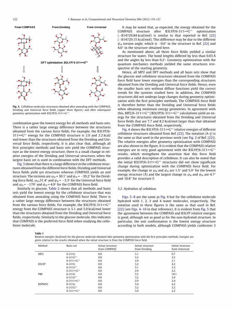
Fig. 3. Cellobiose molecular structures obtained after annealing with the COMPASS,Dreiding and Universal force fields (upper three figures) and after subsequentgeometry optimization with B3LYP/6-311++G⁄⁄.

122 F. Bazooyar et al. / Computational and Theoretical Chemistry 984 (2012) 119–127

combination gave the lowest energy for all methods and basis sets.There is a rather large energy difference between the structuresobtained from the various force fields. For example, the B3LYP/6-311++G⁄⁄ energy for the COMPASS structure is 2.9 and 2.2 kcal/mol lower than the structures obtained from the Dreiding and Uni-versal force fields, respectively. It is also clear that, although allfirst principles methods and basis sets yield the COMPASS struc-ture as the lowest energy structure, there is a small change in rel-ative energies of the Dreiding and Universal structures when thelargest basis set is used in combination with the DFT methods.

Fig. 3 shows that there is a large difference in the cellobiose struc-tures obtained from the different force fields. Dreiding and Universalforce fields yield syn structures whereas COMPASS yields an antistructure. The torsions are uH = 30.1� and wH = �39.2� for the Dreid-ing force field, uH=51.4� and wH = �3.3� for the Universal force fieldand uH = �179� and wH = 4.9� for the COMPASS force field.

Similarly to glucose, Table 2 shows that all methods and basissets yield the lowest energy for the cellobiose structure that wasobtained from annealing using the COMPASS force field. There isa rather large energy difference between the structures obtainedfrom the various force fields. For example, the B3LYP/6-311++G⁄⁄

energy from the COMPASS structure is 5.1 and 5.0 kcal/mol lowerthan the structures obtained from the Dreiding and Universal forcefields, respectively. Similarly to the glucose molecule, this indicatesthat COMPASS is the preferred force field when studying the cello-biose molecule.

Table 1Relative energies (kcal/mol) for the glucose molecule obtained after geogiven relative to the results obtained when the initial structure is from

Method Basis-set Initial structurefrom COMPASS

MP2 6-311G 0.06-311G⁄⁄ 0.06-311++G⁄⁄ 0.0

B3LYP 6-311G 0.06-311G⁄⁄ 0.06-311++G⁄⁄ 0.0

PBE 6-311G 0.06-311G⁄⁄ 0.06-311++G⁄⁄ 0.0

B3PW91 6-311G 0.06-311G⁄⁄ 0.06-311++G⁄⁄ 0.0

It may be noted that, as expected, the energy obtained for theCOMPASS structure after B3LYP/6-311++G⁄⁄ optimization(�814729.84 kcal/mol) is similar to that reported in Ref. [22](�814729.15 kcal/mol). This difference may be due to the differentwH torsion angle, which is �0.6� in the structure in Ref. [22] and4.6� in the structure obtained here.

As mentioned above, all three force fields yielded a similarstructure for water. The bond lengths differed by less than 0.03 Åand the angles by less than 0.2�. Geometry optimization with thequantum mechanics methods yielded the same structures irre-spective of the starting geometry.

Hence, all MP2 and DFT methods and all basis sets show thatthe glucose and cellobiose structures obtained from the COMPASSforce field have lower energies than the corresponding structuresobtained from the Dreiding and Universal force fields. Hence, eventhe smaller basis sets without diffuse functions yield the correcttrends for the systems studied here. In addition, the COMPASSstructures did not undergo large changes during geometry optimi-zation with the first principles methods. The COMPASS force fieldis therefore better than the Dreiding and Universal force fieldswhen obtaining minimum energy geometries. In agreement withthis, MP2/6-311++G⁄⁄//B3LYP/6-311++G⁄⁄ calculations yield an en-ergy for the structures obtained from the Dreiding and Universalforce fields that are 7.7 and 8.2 kcal/mol larger than that obtainedfrom the COMPASS force field, respectively.

Fig. 4 shows the B3LYP/6-311++G⁄⁄ relative energies of differentcellobiose structures obtained from Ref. [22]. The notation (A–J) isthe same as that used in the previous work (see Fig. 2 of Ref. [22]).The relative energies after geometry optimization with COMPASSare also shown in the figure. It is evident that the COMPASS relativeenergies are in very good agreement with the B3LYP/6-311++G⁄⁄

results, which strengthens the assertion that this force fieldprovides a valid description of cellobiose. It can also be noted thatthe initial B3LYP/6-311++G⁄⁄ structures did not show significantchange during optimization with the COMPASS force field. Forexample, the change in uH and wH are 1.5� and 5.9� for the lowestenergy structure (A) and the largest change in uH and wH are 4.7�and 10.8� for structure F.

3.2. Hydration of cellobiose

Figs. 5–8 are the same as Fig. 4 but for the cellobiose moleculehydrated with 1, 2, 3 and 4 water molecules, respectively. Thenotation used in these figures is the same as that used in Ref.[22] (see Figs. 4–10 in that reference). It is evident from Fig. 5 thatthe agreement between the COMPASS and B3LYP relative energiesis good, although not as good as for the non-hydrated structure. Inparticular, the anti conformation is the lowest energy structureaccording to both models, although COMPASS yields conformer 3

metry optimization with the first principles methods. Energies arethe COMPASS force field.

Initial structurefrom Dreiding

Initial structurefrom Universal

3.1 0.73.3 3.22.9 2.13.2 4.23.1 3.32.9 2.23.5 10.13.2 3.62.9 2.43.4 4.23.2 3.23.0 2.2

Table 2Relative energies (kcal/mol) for the cellobiose molecule obtained after geometry optimization with the first principles methods. Energiesare given relative to the results obtained when the initial structure is from the COMPASS force field. �Note that, as described in the text, theresults in the third row are from MP2/6-311++G⁄⁄//B3LYP/6-311++G⁄⁄ calculations.

Method Basis-set Initial structurefrom COMPASS

Initial structurefrom Dreiding

Initial structurefrom Universal

MP2 6-311G 0.0 10.3 11.76-311G⁄⁄ 0.0 9.3 8.5� 6-311++G⁄⁄ 0.0 7.7 8.2

B3LYP 6-311G 0.0 8.6 11.06-311G⁄⁄ 0.0 6.9 11.66-311++G⁄⁄ 0.0 5.1 5.0

PBE 6-311G 0.0 9.3 11.56-311G⁄⁄ 0.0 7.3 12.36-311++G⁄⁄ 0.0 5.4 6.2

B3PW91 6-311G 0.0 8.7 10.76-311G⁄⁄ 0.0 6.8 11.16-311++G⁄⁄ 0.0 5.2 5.7

Fig. 4. Relative energies (kcal/mol) of the non-hydrated cellobiose conformers. TheB3LYP/6-311++G⁄⁄ relative energies are shown as crosses and the COMPASS relativeenergies as triangles.

F. Bazooyar et al. / Computational and Theoretical Chemistry 984 (2012) 119–127 123

as the lowest energy structure and not conformer 1 as predicted byDFT. This is not a significant difference since the energy differencebetween these two conformers is less than 0.3 kcal/mol, irrespec-tive of the model used in the calculation. It is also evident fromthe figure that the COMPASS force field yields the same trends asB3LYP/6-311++G⁄⁄ when progressing from structures 1 through15 (anti conformers) and 16 through 30 (syn conformers). Thereis also good agreement between the molecular structures obtainedfrom the two models. For example, the COMPASS force field yieldsuH = �179.8� and wH = 5.5� for structure 1 (the lowest energystructure according to B3LYP) which can be compared to the DFTvalues of uH = 179.1� and wH = 0.3�. Similarly, the values of struc-ture 3 (the lowest energy structure according to COMPASS) are

Fig. 5. Relative energies (kcal/mol) of the monohydrated cellobiose conformers. The B3energies as triangles. The anti conformers are illustrated in the left panel and the syn in

uH = �179� and wH = 4.9� from COMPASS and uH = 176.7� andwH = �1.3� from B3LYP/6-311++G⁄⁄.

The agreement between the relative energies obtained from theCOMPASS force field and those obtained from B3LYP/6-311++G⁄⁄

are not as good for the di-, tri- and tetrahydrates as it was forthe monohydrate and non-hydrated cellobiose. The main differ-ence between the models is that the COMPASS force field prefersan anti conformer over the syn conformer for all systems whereas,according to the DFT calculations, a syn conformer becomes thelowest energy conformer when the cellobiose is hydrated withtwo or more water molecules. The COMPASS force field does, how-ever, yield the correct trends in energy change within each con-former series. For example, Fig. 6 shows that, according to bothCOMPASS and DFT, the energy increases when going from antistructures 1 through 11 (upper panel) and syn structures 12–20(lower panel) for the dihydrates.

As shown in Fig. 7, the B3LYP/6-311++G⁄⁄ yields increasing rela-tive energies from structure 1 through 5 (anti) and 6 through 10(syn). The COMPASS force field captures these trends, although forsome structures there are up to 2 kcal/mol deviations in relativeenergies. However, the largest difference is that, according to DFT,the lowest energy syn conformer is 0.8 kcal/mol lower than the low-est energy anti conformer, whereas the COMPASS force field favorsthe anti conformer by at least 0.83 kcal/mol over the syn conformers.

Similar behavior is observed for the tetrahydrate (Fig. 8) whereB3LYP/6-311++G⁄⁄ favors the syn conformer (structure 2 in Fig. 8)by 1.2 kcal/mol over the anti structure 1, whereas COMPASS favorsthe anti structure by 0.5 kcal/mol.

Hence, COMPASS does not give the correct trends of favoringsyn over the anti structures for the di-, tri- and tetrahydratesystems. However, it is of interest that the relative difference in

LYP/6-311++G⁄⁄ relative energies are shown as crosses and the COMPASS relativethe right.

Fig. 6. Same as Fig. 5 but for the cellobiose dihydrate.

Fig. 7. Same as Fig. 5 but for the cellobiose trihydrate.

Fig. 8. Same as Fig. 5 but for the cellobiose tetrahydrate. All structures (anti andsyn) are shown in this figure.

Fig. 9. Torsion distribution, uH, of cellobiose in vacuum at 298 K when the initialstructure is syn.

Fig. 10. Torsion distribution, uH, of cellobiose in vacuum at 298 K and 375 K whenthe initial structure is anti.

124 F. Bazooyar et al. / Computational and Theoretical Chemistry 984 (2012) 119–127

the lowest energy syn and lowest energy anti decreases from 1.2through 0.83 to 0.50 as one increases the number of water

molecules from 2 to 4. This raises the question if COMPASS yieldsthe syn conformer when hydrating with a large number of watermolecules. This is discussed below.

3.3. Conformations of cellobiose at elevated temperatures

Strati et al. [16] used the B3LYP/6-311++G⁄⁄method to estimatethe enthalpy and entropy contributions to the Gibbs free energy forvarious cellobiose conformers (in vacuum). There results indicate

Fig. 11. Torsion distribution, uH, of cellobiose in bulk water at 100, 298, 350 and 475 K, when the initial structures are syn (left) and anti (right).

F. Bazooyar et al. / Computational and Theoretical Chemistry 984 (2012) 119–127 125

that the syn conformers have a larger entropy contribution thanthe anti conformers, and may therefore be thermodynamically sta-ble at higher temperatures. To investigate these effects, for cellobi-ose in vacuum and in bulk water, we have performed MDsimulations at various temperatures to ascertain if anti M synisomerization occurs at elevated temperatures. As discussed inSection 2, the simulations in the bulk water were done underNpT conditions where the pressure is 1 bar.

At very low temperatures (e.g., 100 K) the conformer that is ob-served in the simulations depends on the initial cellobiose struc-ture. That is, the syn(anti) conformer is seen when starting withthe syn(anti) structure since the energy barrier for isomerizationhas not been passed within the simulation time. However, this isnot the case for higher temperatures. Fig. 9 shows the distributionof uH when the cellobiose (in vacuum) initially had a syn confor-mation and the temperature is 298 K (wH is not shown since thistorsion does not provide information on anti M syn isomerization).The data shown in the figure were obtained from the last part ofthe simulation, once the syn had isomerized to anti. Note that thesame results were obtained at 325 K, and in neither case did the

anti revert back to the syn. Hence, at these temperatures the anticonformer is thermodynamically stable.

This was confirmed by analyzing the uH distribution when thecellobiose initially had an anti conformation. These results areshown for temperatures of 298 K and 375 K in Fig. 10. It is clearthat the anti conformation remains in this conformation at 298 K,which is expected since this is the thermodynamically stable struc-ture. However, at 375 K there are peaks in the distribution that be-long to both anti and syn conformations. It is important to note thatmultiple barrier crossings occur (i.e., many anti M syn isomeriza-tions occur in the simulation time) showing that both parts ofcoordinate space are sampled at this temperature. As expected,the same behavior is found at even higher temperatures, withthe fraction of time spent in the syn conformation increasing withtemperature. This trend does not depend on which initial con-former is used, and when starting with the anti conformer the frac-tion of time spent in the syn conformer is 0.16, 0.47, 0.57 and 0.70for 375, 400, 425 and 500 K, respectively.

The distributions of uH for cellobiose in bulk water at 1 bar and100, 298, 350 and 475 K are shown in Fig. 11. The results when

126 F. Bazooyar et al. / Computational and Theoretical Chemistry 984 (2012) 119–127

starting from the anti structure are shown in the right panel andthose when starting from the syn structure are shown in the leftpanel. It is clear that, within the simulation time, the anti M synisomerization barrier is not crossed at 100 K and the conformersseen in the simulation are the same as the initial conformer. How-ever, at 298 K and above the anti structure isomerizes to the synconformer, and there are multiple anti M syn barrier crossings.The fraction of time as a syn conformer increases with tempera-ture, and it is 0.42, 0.76, 0.80 and 0.88 at 298, 350, 375 and475 K, respectively. Due to its stability at increased temperatures,the syn conformation remains in this geometry for most of the sim-ulations that begin with this conformation, and a temperature of atleast 475 K is required to obtain a significant (0.20) population ofthe anti structure within the 600 ps simulation time. These resultsshow that, in bulk water at 1 bar, the syn conformer is the pre-ferred conformer at temperatures above 298 K. This is in agree-ment with the B3LYP/6-311++G⁄⁄ results described above andshows that the COMPASS force field is a valid force field whenstudying trends in the cellobiose structure under these conditions.This, in turn, indicates that this force field can be used to studytrends in changes of the cellulose structure under these conditions.

4. Conclusion

Three MM force fields have been evaluated for their use instudying cellulose structural changes in water (such as dissolutionmechanisms). In order to compare with first principles calcula-tions, the study has focused on water, glucose (as the repeatingunit of cellulose) and cellobiose molecules (as the shortest cellu-lose chain), since these molecules allow for first principles calcula-tions in a tractable computational time.

The COMPASS force field is preferred over the Dreiding and Uni-versal force fields since it is the only one of these three force fieldsthat yields the correct anti conformer of cellobiose. In addition, firstprinciples geometry optimizations from the annealed minimumenergy structures of cellobiose and glucose obtained from the threeforce fields shows that the structure obtained from the COMPASSforce field is lowest in energy. Moreover, there are not largechanges of the structures obtained from the COMPASS force fieldduring the first principles optimizations.

Since the COMPASS force field is preferred over the Dreidingand Universal force fields it was used in a more detailed compari-son for the cellobiose molecule hydrated with between 0 and 4water molecules. The comparison was made with relative energiesand structures calculated previously [22] using the B3LYP/6-311++G⁄⁄method. The COMPASS force field yields results for cello-biose that are in excellent agreement with these DFT results. Thequantitative agreement seen for cellobiose deteriorates as morewater molecules are added to the system. For example, the changefrom an anti to a syn minimum energy structure, which is predictedby B3LYP/6-311++G⁄⁄ after hydration with two water molecules, isnot observed with the COMPASS force field. However, the energetictrends within each anti or syn series are predicted, as is the de-crease in the energy of the anti conformer relative to the syn con-former with increasing number of water molecules. In fact,simulations in bulk water at 1 bar and 298 K show that the COM-PASS force field prefers the syn structure, indicating that this forcefield yields valid trends in structural changes under theseconditions.

In agreement with B3LYP/6-311++G⁄⁄, the COMPASS force fieldalso shows that the syn conformer is favored over the anti con-former for cellobiose (in vacuum) at high temperatures. Thereare multiple crossings of the isomerization barrier at high temper-atures, and the fraction of time when the cellobiose is in the synconformation increases with increasing temperature.

Acknowledgements

The authors are grateful to Stiftelsen FöreningssparbankenSjuhärad for financial support. The Quantum Mechanics calcula-tions were performed on resources provided by the Swedish Na-tional Infrastructure for Computing (SNIC) at NSC, HPC2N andC3SE. Molecular Mechanics results were obtained using programfrom Accelrys Software Inc.

References

[1] Europe’s energy portal, downloaded on October 2010 from <http://www.energy.eu/>.

[2] P.F.H. Harmsen, W.J.J. Huijgen, L.M. Bermúdez López, R.R.C. Bakker. Literaturereview of physical and chemical pretreatment processes for lignocellulosic,biomass, ECN-E-10-013, 2010.

[3] P. Stroeve, P. Kumar, D.M. Barrett, M.J. Delwiche, Methods for pretreatment oflignocellulosic biomass for efficient hydrolysis and biofuel production, Ind.Eng. Chem. Res. 48 (2009) 3713–3729.

[4] M. Ladisch, N. Mosier, C. Wyman, B. Dale, R. Elander, Y.Y. Lee, M. Holtzapple,Features of promising technologies for pretreatment of lignocellulosicbiomass, J. Bioresource Technol. 96 (6) (2005) 673–686.

[5] MJ. Taherzadeh, K. Karimi, Pretreatment of lignocellulosic wastes to improveethanol and biogas production: a review, Int. J. Mol. Sci. 9 (2008) 1621–1651.

[6] M.J. Taherzadeh, K. Karimi, Acid-based hydrolysis processes for ethanol fromlignocellulosic materials: a review, J. Bioresources 2 (2007) 707–738.

[7] Shi.-You. Ding, Michael.E. Himmel, The maize primary cell wall microfibril: anew model derived from direct visualization, J. Agric. Food Chem. 54 (2006)597–606.

[8] D. Mohnen, M. Bar-Peled, C. Somerville, Cell wall polysaccharide synthesis, in:M.E. Himmel (Ed.), Biomass Recalcitrance: Deconstructing the Plant Cell Wallfor Bioenergy, Blackwell Publisher, 2008 (Chapter 5).

[9] M.F. Crowley, R.C. Walker, Computational approaches to study cellulosehydrolysis, in: M.E. Himmel (Ed.), Biomass Recalcitrance: Deconstructing thePlant Cell Wall for Bioenergy, Blackwell Publishing, 2008 (Chapter 8).

[10] A.D. French, D.P. Miller, A. Aabloo, Miniature crystal models of cellulosepolymorphs and other carbohydrates, Int. J. Biol. Macromol. 15 (1) (1993) 30–36.

[11] A.P. Heiner, O. Teleman, Interface between monoclinic crystalline cellulose andwater: breakdown of the odd/even duplicity, J. Langmuir 13 (1997) 511–518.

[12] A.P. Heiner, L. Kuutti, O. Teleman, Comparison of the interface between waterand four surfaces of native crystalline cellulose by molecular dynamicssimulations, Carbohydr. Res. 306 (1–2) (1998) 205–220.

[13] S. Neyertz, A. Pizzi, A. Merlin, B. Maigret, D. Brown, X. Deglise, A new all-atomforce field for crystalline cellulose I, J. Appl. Polym. Sci. 78 (11) (2000) 1939–1946.

[14] O. Biermann, F. Müller-Plathe, E. Hädicke, S. Koltzenburg, Hydrophilicity andlipophilicity of cellulose crystal surfaces, Angew. Chem. Int. Ed. 40 (20) (2001)3822–3825.

[15] Y. Nishiyama, P. Langan, H. Chanzy, Crystal structure and hydrogen-bondingsystem in cellulose Ib from synchrotron X-ray and neutron fiber diffraction, J.Am. Chem. Soc. 124 (31) (2002) 9074–9082.

[16] G.L. Strati, J.L. Willett, F.A. Momany, Ab initio computational study of b-cellobiose conformers using B3LYP/6-311++G⁄⁄, Carbohydr. Res. 337 (20)(2002) 1833–1849.

[17] K. Mazeau, L. Heux, Molecular dynamics simulations of bulk native crystallineand amorphous structures of cellulose, J. Phys. Chem. B 107 (10) (2003) 2394–2403.

[18] Y. Nishiyama, J. Sugiyama, H. Chanzy, P. Langan, Crystal structure andhydrogen bonding system in cellulose Ia from synchrotron X-ray andneutron fiber diffraction, J. Am. Chem. Soc. 125 (47) (2003) 14300–14306.

[19] J.W. Brady, M.E. Himmel, J.F. Matthews, C.E. Skopec, P.E. Mason, P. Zuccato,R.W. Torget, J. Sugiyama, Computer simulation studies of microcrystallinecellulose Ib, Carbohydr. Res. 341 (1) (2006) 138–152.

[20] A.D. French, Z.M. Ford, E.D. Stevens, G.P. Johnson, Determining the crystalstructure of cellulose III(I) by modeling, Carbohydr. Res. 340 (5) (2005) 827–833.

[21] F. Tanaka, K. Okamura, Characterization of cellulose molecules in bio-systemstudied by modeling methods, Cellulose 12 (3) (2005) 243–252.

[22] W.B. Bosma, M. Appell, J.L. Willett, F.A. Momany, Stepwise hydration ofcellobiose by DFT methods: 1. Conformational and structural changes broughtabout by the addition of one to four water molecules, J. Mol. Struct:THEOCHEM 776 (1-3) (2006) 1–19.

[23] T. Yui, S. Nishimura, S. Akiba, S. Hayashi, Swelling behavior of the cellulose Ibcrystal models by molecular dynamics, Carbohydr. Res. 341 (15) (2006) 2521–2530.

[24] M. Bergenstråhle, J. Wohlert, P.T. Larsson, K. Mazeau, L.A. Berglund, Dynamicsof cellulose-water interfaces: NMR spin-lattice relaxation times calculatedfrom atomistic computer simulations, J. Phys. Chem. B 112 (9) (2008) 2590–2595.

[25] T. Yui, S. Hayashi, Molecular dynamics simulations of solvated crystal modelsof cellulose Ia and IIII, Biomacromolecules 8 (3) (2007) 817–824.

F. Bazooyar et al. / Computational and Theoretical Chemistry 984 (2012) 119–127 127

[26] M. Bergenstråhle, K. Mazeau, L.A. Berglund, Molecular modeling of interfacesbetween cellulose crystals and surrounding molecules: effects of caprolactonesurface grafting, Eur. Polym. J. 44 (11) (2008) 3662–3669.

[27] A. Jeihanipour, MJ. Taherzadeh, Ethanol production from cotton-based wastetextiles, J. Bioresour. Technol. 100 (2) (2009) 1007–1010.

[28] C.A. Stortz, G.P. Johnson, A.D. French, G.I. Csonka, Comparison of different forcefields for the study of disaccharides, J. Carbohydr. Res. 344 (2009) 2217–2228.

[29] D. Zin-Eddine, P.Q. José, Acid hydrolysis of cellulose. Part II: stochasticsimulation using a monte carlo technique, Can. J. Chem. Eng. 72 (1) (1994)106–112.

[30] M. Bergenstråhle, J. Matthews, M. Crowley, J. Brady. Cellulose crystal structureand force fields, downloaded on December 2010 <http://www.tappi.org/content/events/10nano/papers/12.5.pdf>

[31] P. Aldred, Atomistic modeling of the complex interactions of cellulose I and IIpolymorphs, downloaded on December 2010: <http://www.accelrys.com/resource-center/case-studies/archive/studies/cellulose.html>.

[32] H. Sun, COMPASS: an ab initio force-field optimized for condensed-phaseapplications overview with details on alkane and benzene compounds, J. Phys.Chem. B 102 (38) (1998) 7338–7364.

[33] S.L. Mayo, B.D. Olafson, W.A. Goddard, Dreiding: a general force field formolecular simulation, J. Phys. Chem. 94 (26) (1990) 8897–8909.

[34] A.K. Rappe, C.J. Casewit, K.S. Colwell, W.A. Goddard, W.M. Skiff, UFF, a fullperiodic table force field for molecular mechanics and molecular dynamicssimulations, J. Am. Chem. Soc. 114 (25) (1992) 10024–10035.

[35] F.A. Momany, U. Schnupf, DFTMD studies of b-cellobiose: conformationalpreference using implicit solvent, J. Carbohydr. Res. 346 (5) (2011) 619–630.

[36] A.D. Becke, Density-functional thermochemistry. III. The role of exactexchange, J. Chem. Phys. 98 (7) (1993) 5648.

[37] C. Lee, W. Yang, R.G. Parr, Development of the Colle–Salvetti correlation-energy formula into a functional of the electron density, Phys. Rev. B 37 (1998)785–789.

[38] B. Miehlich, A. Savin, H. Stoll, H. Preuss, Results obtained with the correlationenergy density functionals of Becke and Lee, Yang and Parr., Chem. Phys. Lett.157 (3) (1989) 200–206..

[39] P.J. Stephens, F.J. Devlin, C.F. Chabalowski, M.J. Frisch, Ab Initio calculation ofvibrational absorption and circular dichroism spectra using density functionalforce fields, J. Phys. Chem. 98 (45) (1994) 11623–11627.

[40] J.P. Perdew, K. Burke, M. Ernzerhof, Generalized gradient approximation madesimple, Phys. Rev. Lett. 77 (18) (1996) 3865–3868.

[41] J.P. Perdew, Y. Wang, Accurate and simple analytic representation of theelectron-gas correlation energy, J. Phys. Rev. B 45 (1992) 13244–13249.

[42] M.J. Frisch, G.W. Trucks, H.B. Schlegel, G.E. Scuseria, M.A. Robb, J.R. Cheeseman,G. Scalmani, V. Barone, B. Mennucci, G.A. Petersson, H. Nakatsuji, M. Caricato,X. Li, H.P. Hratchian, A.F. Izmaylov, J. Bloino, G. Zheng, J.L. Sonnenberg, M.Hada, M. Ehara, K. Toyota, R. Fukuda, J. Hasegawa, M. Ishida, T. Nakajima, Y.Honda, O. Kitao, H. Nakai, T. Vreven, J.A. Montgomery, Jr., J.E. Peralta, F. Ogliaro,M. Bearpark, J.J. Heyd, E. Brothers, K.N. Kudin, V.N. Staroverov, R. Kobayashi, J.Normand, K. Raghavachari, A. Rendell, J.C. Burant, S. S. Iyengar, J. Tomasi, M.Cossi, N. Rega, J.M. Millam, M. Klene, J.E. Knox, J.B. Cross, V. Bakken, C. Adamo,J. Jaramillo, R. Gomperts, R.E. Stratmann, O. Yazyev, A.J. Austin, R. Cammi, C.Pomelli, J.W. Ochterski, R.L. Martin, K. Morokuma, V.G. Zakrzewski, G.A. Voth,P. Salvador, J.J. Dannenberg, S. Dapprich, A.D. Daniels, Ö. Farkas, J.B. Foresman,J.V. Ortiz, J. Cioslowski, D.J. Fox, Gaussian 09, Revision A.02, Gaussian, Inc.,Wallingford CT, 2009.

[43] J.H. Lii, B. Ma, N.L. Allinger, Importance of selecting proper basis set inquantum mechanical studies of potential energy surfaces of carbohydrates, J.Comput. Chem 20 (15) (1999) 1593–1603.

[44] J.R. Freid, Computational parameters, in: A.E. Mark (Ed.), Physical Properties ofPolymers Handbook, second ed., Springer Publisher, 2006, pp. 63–64 (Chapter 4).

[45] S.W. Bunte, H. Sun, Molecular modeling of energetic materials: theparameterization and validation of nitrate esters in the COMPASS force field,J. Phys. Chem. B 104 (11) (2000) 2477–2489.

[46] T.C. Lim, R.A. Udyavara, Relations between Varshni and Morse potential energyparameters, Central Eur. J. Phys. 7 (1) (2009) 193–197.

[47] J. S. Conery, W. L. Peticolas, T. Rush III, K. Shanmugam, J. Dominguez, A parallelalgorithm for calculating the potential energy in DNA, HICSS, in: 28th HawaiiInternational Conference on System Sciences (HICSS’95), 1995, pp.123.

[48] A.D. French, G.P. Johnson, Advanced conformational energy surfaces forcellobiose, Cellulose 11 (3-4) (2004) 449–462.

[49] U. Schnupf, F.A. Momany, Rapidly calculated DFT relaxed iso-potential //wmaps: b-cellobiose, Cellulose 18 (2011) 859–887.

[50] O. Guvench, E. Hatcher, R.M. Venable, R.W. Pastor, A.D. MacKerell Jr, CHARMMAdditive all-atom force field for glycosidic linkages between hexopyranoses, J.Chem. Theory Comput. 20 (5) (2009) 2353–2370.

[51] R.K. Campen, A.V. Verde, J.D. Kubicki, Influence of glycosidic linkage neighborson disaccharide conformation in vacuum, J. Phys. Chem. B 111 (49) (2007)13775–13785.

Paper II

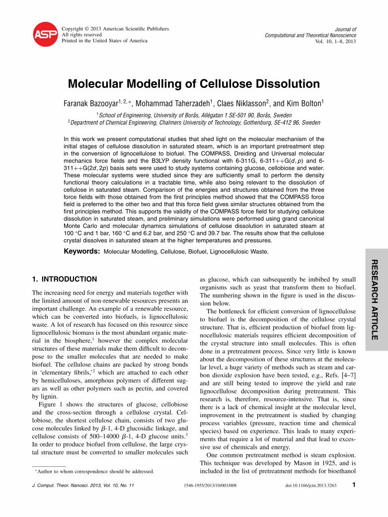
RESEARCH

ARTIC

LE

Copyright © 2013 American Scientific PublishersAll rights reservedPrinted in the United States of America

Journal ofComputational and Theoretical Nanoscience

Vol. 10, 1–8, 2013

Molecular Modelling of Cellulose Dissolution

Faranak Bazooyar1�2�∗, Mohammad Taherzadeh1, Claes Niklasson2, and Kim Bolton11School of Engineering, University of Borås, Allégatan 1 SE-501 90, Borås, Sweden

2Department of Chemical Engineering, Chalmers University of Technology, Gothenburg, SE-412 96, Sweden

In this work we present computational studies that shed light on the molecular mechanism of theinitial stages of cellulose dissolution in saturated steam, which is an important pretreatment stepin the conversion of lignocellulose to biofuel. The COMPASS, Dreiding and Universal molecularmechanics force fields and the B3LYP density functional with 6-311G, 6-311++G(d,p) and 6-311++G(2d, 2p) basis sets were used to study systems containing glucose, cellobiose and water.These molecular systems were studied since they are sufficiently small to perform the densityfunctional theory calculations in a tractable time, while also being relevant to the dissolution ofcellulose in saturated steam. Comparison of the energies and structures obtained from the threeforce fields with those obtained from the first principles method showed that the COMPASS forcefield is preferred to the other two and that this force field gives similar structures obtained from thefirst principles method. This supports the validity of the COMPASS force field for studying cellulosedissolution in saturated steam, and preliminary simulations were performed using grand canonicalMonte Carlo and molecular dynamics simulations of cellulose dissolution in saturated steam at100 �C and 1 bar, 160 �C and 6.2 bar, and 250 �C and 39.7 bar. The results show that the cellulosecrystal dissolves in saturated steam at the higher temperatures and pressures.

Keywords: Molecular Modelling, Cellulose, Biofuel, Lignocellulosic Waste.

1. INTRODUCTION

The increasing need for energy and materials together withthe limited amount of non-renewable resources presents animportant challenge. An example of a renewable resource,which can be converted into biofuels, is lignocellulosicwaste. A lot of research has focused on this resource sincelignocellulosic biomass is the most abundant organic mate-rial in the biosphere,1 however the complex molecularstructures of these materials make them difficult to decom-pose to the smaller molecules that are needed to makebiofuel. The cellulose chains are packed by strong bondsin ‘elementary fibrils,’2 which are attached to each otherby hemicelluloses, amorphous polymers of different sug-ars as well as other polymers such as pectin, and coveredby lignin.Figure 1 shows the structures of glucose, cellobiose

and the cross-section through a cellulose crystal. Cel-lobiose, the shortest cellulose chain, consists of two glu-cose molecules linked by �-1, 4-D glucosidic linkage, andcellulose consists of 500–14000 �-1, 4-D glucose units.3

In order to produce biofuel from cellulose, the large crys-tal structure must be converted to smaller molecules such

∗Author to whom correspondence should be addressed.

as glucose, which can subsequently be imbibed by smallorganisms such as yeast that transform them to biofuel.The numbering shown in the figure is used in the discus-sion below.The bottleneck for efficient conversion of lignocellulose

to biofuel is the decomposition of the cellulose crystalstructure. That is, efficient production of biofuel from lig-nocellulosic materials requires efficient decomposition ofthe crystal structure into small molecules. This is oftendone in a pretreatment process. Since very little is knownabout the decomposition of these structures at the molecu-lar level, a huge variety of methods such as steam and car-bon dioxide explosion have been tested, e.g., Refs. [4–7]and are still being tested to improve the yield and ratelignocellulose decomposition during pretreatment. Thisresearch is, therefore, resource-intensive. That is, sincethere is a lack of chemical insight at the molecular level,improvement in the pretreatment is studied by changingprocess variables (pressure, reaction time and chemicalspecies) based on experience. This leads to many experi-ments that require a lot of material and that lead to exces-sive use of chemicals and energy.One common pretreatment method is steam explosion.

This technique was developed by Mason in 1925, and isincluded in the list of pretreatment methods for bioethanol

J. Comput. Theor. Nanosci. 2013, Vol. 10, No. 11 1546-1955/2013/10/001/008 doi:10.1166/jctn.2013.3263 1

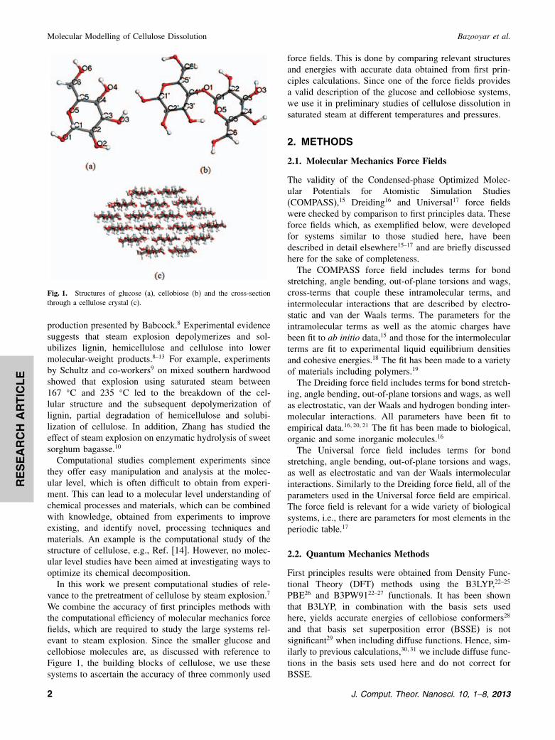
RESEARCH

ARTIC

LE

Molecular Modelling of Cellulose Dissolution Bazooyar et al.

Fig. 1. Structures of glucose (a), cellobiose (b) and the cross-sectionthrough a cellulose crystal (c).

production presented by Babcock.8 Experimental evidencesuggests that steam explosion depolymerizes and sol-ubilizes lignin, hemicellulose and cellulose into lowermolecular-weight products.8–13 For example, experimentsby Schultz and co-workers9 on mixed southern hardwoodshowed that explosion using saturated steam between167 �C and 235 �C led to the breakdown of the cel-lular structure and the subsequent depolymerization oflignin, partial degradation of hemicellulose and solubi-lization of cellulose. In addition, Zhang has studied theeffect of steam explosion on enzymatic hydrolysis of sweetsorghum bagasse.10

Computational studies complement experiments sincethey offer easy manipulation and analysis at the molec-ular level, which is often difficult to obtain from experi-ment. This can lead to a molecular level understanding ofchemical processes and materials, which can be combinedwith knowledge, obtained from experiments to improveexisting, and identify novel, processing techniques andmaterials. An example is the computational study of thestructure of cellulose, e.g., Ref. [14]. However, no molec-ular level studies have been aimed at investigating ways tooptimize its chemical decomposition.In this work we present computational studies of rele-

vance to the pretreatment of cellulose by steam explosion.7

We combine the accuracy of first principles methods withthe computational efficiency of molecular mechanics forcefields, which are required to study the large systems rel-evant to steam explosion. Since the smaller glucose andcellobiose molecules are, as discussed with reference toFigure 1, the building blocks of cellulose, we use thesesystems to ascertain the accuracy of three commonly used

force fields. This is done by comparing relevant structuresand energies with accurate data obtained from first prin-ciples calculations. Since one of the force fields providesa valid description of the glucose and cellobiose systems,we use it in preliminary studies of cellulose dissolution insaturated steam at different temperatures and pressures.

2. METHODS

2.1. Molecular Mechanics Force Fields

The validity of the Condensed-phase Optimized Molec-ular Potentials for Atomistic Simulation Studies(COMPASS),15 Dreiding16 and Universal17 force fieldswere checked by comparison to first principles data. Theseforce fields which, as exemplified below, were developedfor systems similar to those studied here, have beendescribed in detail elsewhere15–17 and are briefly discussedhere for the sake of completeness.The COMPASS force field includes terms for bond

stretching, angle bending, out-of-plane torsions and wags,cross-terms that couple these intramolecular terms, andintermolecular interactions that are described by electro-static and van der Waals terms. The parameters for theintramolecular terms as well as the atomic charges havebeen fit to ab initio data,15 and those for the intermolecularterms are fit to experimental liquid equilibrium densitiesand cohesive energies.18 The fit has been made to a varietyof materials including polymers.19

The Dreiding force field includes terms for bond stretch-ing, angle bending, out-of-plane torsions and wags, as wellas electrostatic, van der Waals and hydrogen bonding inter-molecular interactions. All parameters have been fit toempirical data.16�20�21 The fit has been made to biological,organic and some inorganic molecules.16

The Universal force field includes terms for bondstretching, angle bending, out-of-plane torsions and wags,as well as electrostatic and van der Waals intermolecularinteractions. Similarly to the Dreiding force field, all of theparameters used in the Universal force field are empirical.The force field is relevant for a wide variety of biologicalsystems, i.e., there are parameters for most elements in theperiodic table.17

2.2. Quantum Mechanics Methods

First principles results were obtained from Density Func-tional Theory (DFT) methods using the B3LYP,22–25

PBE26 and B3PW9122–27 functionals. It has been shownthat B3LYP, in combination with the basis sets usedhere, yields accurate energies of cellobiose conformers28

and that basis set superposition error (BSSE) is notsignificant29 when including diffuse functions. Hence, sim-ilarly to previous calculations,30�31 we include diffuse func-tions in the basis sets used here and do not correct forBSSE.

2 J. Comput. Theor. Nanosci. 10, 1–8, 2013

RESEARCH

ARTIC

LE

Bazooyar et al. Molecular Modelling of Cellulose Dissolution

Some of the results, including those obtained frompost-Hartree Fock Moller-Plesset second order correlationenergy correction (MP2) have been presented elsewhere,32

and here we only show results obtained from the B3LYPfunctional with basis sets that yield accurate structuresand energies for glucose and cellobiose. In particular,we use B3LYP/6-311++G(d,p) for systems containingonly glucose or cellobiose molecules and B3LYP/6-311++G(2d, 2p) when water is included in the glucosesystem. The 6-311G basis set was used for systems con-taining two cellobiose molecules and water due to compu-tational constraints.

2.3. Simulation Methods

The three molecular mechanics force fields discussedabove were used to anneal the molecular structure of cel-lobiose, glucose and water to identify the global minimumenergy structures. Although one cannot prove that one haslocated the global energy minimum, the annealed mini-mum energy structures obtained in this study are not sen-sitive to the annealing temperatures, simulation lengths orinitial geometries since sufficiently high mid-cycle tem-peratures and sufficiently long annealing simulations havebeen performed. The fact that the same annealed struc-tures are obtained under all proper conditions indicatesthat this structure is the chemically relevant minimum, andthat the annealing conditions allowed for complete sam-pling of coordination space. Typical annealing simulationsconsisted of 50–70 cycles with about 5 million simula-tion steps per cycle (1.0 fs time steps) and mid-cycle tem-peratures of 400–500 K for cellobiose and glucose and250 K for water. The molecular geometry was optimizedto its minimum energy structure at the end of each cycle.The structures were considered to be minimized once thechange in energy between subsequent optimization stepswas less than 2�0×10−5 kcal/mol.

The annealed structures were subsequently used as theinput for the first principles minimum energy optimiza-tions. In principle this would be nine structures (a cel-lobiose, glucose and water structure for each of the threeforce fields), but the force fields yielded very similar struc-tures for water, which means that only seven structureswere used for the first principles calculations. These cal-culations were used to determine which of the molecularmechanics force fields yield the preferred (lowest energy)structure of the cellobiose and glucose molecules.As discussed below, the COMPASS force field is in bet-

ter agreement with the first principles results comparedto the other two force fields, and was therefore used tostudy larger systems containing two glucose or two cel-lobiose molecules, where their interaction with water isalso studied. Similar annealing simulations to those dis-cussed above were used for these larger systems in order tofind the global minimum energy structures. The annealed

structures were subsequently used as input for first princi-ples minimum energy optimizations.The COMPASS force field was also used in preliminary

studies of the solubility of cellulose in saturated steam.The grand canonical Monte Carlo (GCMC) method wasused obtain structures of cellulose crystals in water at dif-ferent temperatures and pressures. A cellulose crystal con-taining eighteen molecular chains (the first two inner shellsof the structure shown in Fig. 1) where each chain con-sisted of three cellobiose units was placed in a 48 Å×50 Å× 35 Å periodic box. The box is sufficiently largeto avoid interaction of the cellulose crystal with its peri-odic images. It is expected that the mechanism of cellu-lose dissolution observed with this eighteen chain modelis relevant to that with all thirty six chains, since thesmaller model also has an inner and outer shell of cellu-lose molecules. It can also be noted that simulations per-formed on crystals composed of eighteen chains with onecellobiose unit in each chain gave similar results to thosepresented here, supporting the fact that a chain length ofthree cellobiose units gives valid results.The results obtained at 100 �C–1 bar, 160 �C–6.2 bar

and 250 �C–39.7 bar combinations are discussed here sincethe second and third conditions have been used in experi-mental studies of steam explosion7 and the first conditionis to see the trend of effect of increasing pressure andtemperature. Since the computational code used here doesnot allow for relaxation of the cellulose structure wheninserting the water molecules during GCMC, the structuresobtained for each temperature and pressure were simulatedusing NpT molecular dynamics (MD) under the same con-ditions used in the GCMC. Trajectories were propagatedfor typically 300 ps using a time-step of 1 fs. Integra-tion was performed using the Verlet algorithm, which hasthe strength of being time-reversible.33 The distance of thecentre of mass of each chain to the centre of mass of thecellulose crystal was monitored so that dissolution of thecrystal could be analysed, once the average density wasconstant.

3. RESULTS AND DISCUSSION

The global minimum energy structures of glucose obtainedfrom the three force fields are shown in the left col-umn of Figure 2, and the corresponding B3LYP struc-tures after further geometry optimisation are shown inthe right column. The main difference in glucose struc-tures obtained from each of the force fields are the OHand CHOH rotations. This is expected since these rota-tions do not have a large energy barrier and the differ-ence in energy between these conformations (for a givenforce field) is small. However, it must be reiterated thatthe structures shown in Figure 2 are the minimum energystructures obtained for each force field. Torsion anglesthat exemplify these differences are given in Table I. For

J. Comput. Theor. Nanosci. 10, 1–8, 2013 3

RESEARCH

ARTIC

LE

Molecular Modelling of Cellulose Dissolution Bazooyar et al.

Fig. 2. Global minimum energy structures of glucose obtained from theCOMPASS, Dreiding and Universal force fields (left) and the B3LYPstructures after subsequent geometry optimisation (right).

example, the O6C6C5O5 torsion is 174�, 173� and 59�

for the COMPASS, Dreiding and Universal force fields,respectively, and the H4O4C4C5 torsion is 172�, −48� and−155� for these force fields.The annealed structures obtained from the COMPASS

force field do not show significant change during furtheroptimization with B3LYP. The change in bond lengthsduring optimization is typically less than 0.02 Å and thechange in bond angles less than 2�. The structure obtainedfrom the Universal force field shows a large change onfurther optimization with B3LYP (where the H-O2C2C3and C2C3O3-H group rotates). These changes are alsoshown in Table I. For example, the H-O2C2C3 torsionis −61� after annealing with the Dreiding force field andit changes to −51� after subsequent geometry optimisa-tion with B3LYP, and the H-O2C2C3 torsion is −79� afterannealing with the Universal force field and it changesto −179� after subsequent B3LYP geometry optimisa-tion. The good agreement between the structure obtainedfrom the COMPASS force field and that obtained after

Table I. Torsion angles (in degrees) of the glucose molecule obtained after annealing using the COMPASS, Dreiding and Universal force fields, andthese angles after subsequent geometry optimisation (G.O.) with B3LYP. The atom numbers are given in Figure 1.

Torsion B3LYP G.O. from B3LYP G.O. from B3LYP G.O. fromangle COMPASS Dreiding Universal COMPASS Dreiding Universal

O6C6C5O5 174 173 59 166 −177 73O1C1O5C5 176 179 175 179.8 −179 179H-O2C2C3 177 −61 −79 −178 −51 −179H-O4C4C5 172 −48 −155 173 −49 170O3C3C4O4 −60 −65 −69 −63 −64 −64C2C3O3-H −60 −177 −156 −50 179 −84

subsequent geometry optimisation with B3LYP supportsthe validity of this force field when studying glucose andshows that the COMPASS force field is preferred to theDreiding and Universal force fields when studying thismolecule.This conclusion is supported by comparing the ener-

gies of the structures optimised by B3LYP. The energyof the structure that is geometry optimised from thatobtained after annealing with the COMPASS force fieldis −431352.65 kcal mol−1 which is lower than the ener-gies of the other two structures, which are −431349.8 and−431350.49 kcal mol−1 for the structures obtained afterannealing with the Dreiding and Universal force fields,respectively. Hence, the glucose structure obtained fromthe COMPASS force field not only has a structure that isin good agreement with B3LYP, but it is also the energet-ically preferred structure.Figure 3 is the same as Figure 2 but for cellobiose.

Similarly to the results for glucose, the three force fieldsyield different structures for the cellobiose molecule. Oneof the largest differences is that the COMPASS force fieldyields a bent, out-of-plane structure (also called an anticonformer) whereas the other two force fields yield planer(syn) conformers. This is also seen by comparing theH1C1O1C4′ torsion angle, which is −179� for the COM-PASS force field and and 30.1� and 51.4� for the Dreidingand Universal force fields. This, and other torsion anglesthat exemplify differences in the structures, is given inTable II.Figure 3 and the torsion angles shown in Table II illus-

trate that the cellobiose structures change when optimisingwith B3LYP. However, these changes are smaller for thestructure obtained from the COMPASS force field com-pared to those obtained from the other two force fields.For example, the structure obtained from the Dreidingforce field shows large changes in the H4′C4′O1C1 andC1O1C4′C5′ torsion angles, and the structure obtainedfrom the Universal force field shows large changes in theH4′C4′O1C1 and C1O1C4′C5′ torsion angles. Similarlyto the result obtained for glucose, the good agreementbetween the structure obtained from the COMPASS forcefield and that obtained after subsequent geometry optimi-sation with B3LYP supports the validity of this force fieldwhen studying cellobiose and shows that the COMPASS

4 J. Comput. Theor. Nanosci. 10, 1–8, 2013

RESEARCH

ARTIC

LE

Bazooyar et al. Molecular Modelling of Cellulose Dissolution

Fig. 3. Same as Figure 2 but for the cellobiose molecule.

force field is preferred to the Dreiding and Universal forcefields when studying this molecule.This conclusion is also supported by comparing the

energies of the structures optimised by B3LYP. The ener-gies of the cellobiose structures that are geometry opti-mised using B3LYP and when starting with structuresobtained after annealing with the COMPASS, Dreidingand Universal force fields are −814729.84, −814724.72and −814724.83 kcal mol−1, respectively. Hence, the cel-lobiose structure obtained from the COMPASS force fieldnot only has a structure that is in good agreement withB3LYP, but it is also the energetically preferred structure.Since the COMPASS force field gave the preferred glu-

cose and cellobiose structures compared to the Dreidingand Universal force fields and since these structures arein good agreement with the B3LYP results, it was used tostudy the binding strength between two glucose and twocellobiose molecules. This binding strength is expected tobe important when dissolving cellulose in a pretreatmentprocess. The glucose–glucose and cellobiose–cellobiosestructures obtained from annealing with the COMPASS

Table II. Same as Table I but for the cellobiose molecule.

Torsion B3LYP G.O. from B3LYP G.O. from B3LYP G.O. fromangle COMPASS Dreiding Universal COMPASS Dreiding Universal

O6′C6′C5′O5′ −64 171 58 −59 161 58O6C6C5O5 −53 64 59 −59 70 62H-O1′C1′O5′ −30 −60 −74 −67 −67 −71O2′C2′C3′O3′ 58 −65 67 62 65 65O2C2C3O3 56 65 68 61 66 65O3C3O4C4 −62 −66 −68 −64 −63 −64H-O2C2C1 68 57 81 78 51 68H1C1O1C4′ −179 30 51 179 35 33H4′C4′O1C1 4.9 −39 3.3 −0.5 −18 −45C1O1C4′C5′ −115 −156 −118 −120 −137 −163O5C1O1C4′ 63 −92 −71 61 −85 −87

force field are shown in the left column of Figure 4,and the structures after further geometry optimisation withB3LYP are shown in the right column. There is very littlechange in the structure after geometry optimisation. Forexample, the glucose–glucose and cellobiose–cellobiosecentre of mass distances are 5.16 and 4.52 Å after anneal-ing, and they change to 5.36 and 4.31 Å after geom-etry optimisation. The glucose–glucose and cellobiose–cellobiose binding energies are 13 and 29 kcal mol−1

according to the COMPASS force field and 14 and 41.6kcal mol−1 according to B3LYP. Hence, both methodsyield strong binding between the molecules, indicatingthe COMPASS will produce valid mechanisms and trendswhen studying the formation and breaking of glucose–glucose and cellobiose–cellobiose intermolecular bonds.The COMPASS force field was also used the study the

interaction of glucose–glucose and cellobiose–cellobiosepairs with a water molecule (which is important for cellu-lose dissolution in water and steam explosion). Figure 5(a)shows the initial structures that were used for geom-etry optimisation with the COMPASS force field. Thefirst three of these structures were based on the glucose–glucose annealed structure shown in Figure 4, and thefourth structure is based on the glucose–glucose structurethat is often assumed for the cellulose crystal (see Fig. 1).The structures obtained after geometry optimisation (withthe COMPASS force field) are shown in Figure 5(b). Com-parison between the structures in panels (a) and (b) showsthat the preferred location of the water molecule is out-side, and not between, the glucose–glucose pair. This isconfirmed by the structure obtained from simulated anneal-ing with the COMPASS force field and that is shown inFigure 5(c). As shown in Figure 5(d), subsequent geometryoptimisation with B3LYP does not lead to a large changein the geometry. For example, the distances between thecentres of mass of the water-glucose (for the upper glucosein Fig. 5(c)), water-glucose (lower glucose) and glucose–glucose are 2.19, 2.20 and 0.19 Å for the COMPASS struc-ture and 2.42, 2.44 and 0.18 Å for the B3LYP structure.Hence, the COMPASS force field shows that water doesnot prefer to penetrate between two glucose molecules, and

J. Comput. Theor. Nanosci. 10, 1–8, 2013 5

RESEARCH

ARTIC

LE

Molecular Modelling of Cellulose Dissolution Bazooyar et al.

Fig. 4. Glucose–glucose and cellobiose–cellobiose structures obtainedfrom the COMPASS force field (left) and after subsequent geometry opti-misation with B3LYP (right).

Fig. 5. Glucose–glucose pair interacting with a water molecule, struc-tures initially used for geometry optimisation with the COMPASS forcefield (a), after geometry optimisation (b) and simulated annealing (c) withthis force field, and after geometry optimisation of the annealed structurewith B3LYP (d).

Fig. 6. Global minimum energy structure of a cellobiose–cellobiosepair interacting with a water molecule obtained from the COMPASS forcefield (left) and after further geometry optimisation with B3LYP (right).

the annealed structure obtained from the COMPASS forcefield is in good agreement with that obtained after fur-ther geometry optimisation with B3LYP. Once again, thissupports the validity of this force field to study systemscontaining glucose and water molecules.The global minimum energy structure of a cellobiose–

cellobiose pair interacting with a water molecule obtainedafter annealing with the COMPASS force field is shownon the left in Figure 6, and the corresponding B3LYPstructure after further geometry optimisation is shown onthe right. Similarly to the results shown for glucose inFigures 5(c) and (d), the water molecule does not pre-fer to penetrate into the cellobiose–cellobiose pair, but israther located on the outside of the pair. Hence, dissolu-tion of cellulose with water is not expected to be driven bychanges in the system energy. Also, subsequent geometryoptimisation with B3LYP does not lead to a large changein the geometry. For example, the distances between thecentres of mass of the water-cellobiose (for the upper cel-lobiose in Fig. 6), water-cellobiose (lower cellobiose) andcellobiose–cellobiose are 1.99, 2.01 and 0.14 Å for theCOMPASS structure and 2.10, 2.12 and 0.138 Å for theB3LYP structure.Typical snap shots obtained after NpT equilibration at

100 �C and 1 bar, 160 �C and 6.2 bar and 250 �C and 39.7bar are shown in Figure 7. The water molecules are shownin blue, the cellulose chains that were initially in the innercrystal shell in green and the chains that were initially inthe outer shell in red. These temperature–pressure (T –p)combinations were chosen since they have been used inexperimental steam explosion studies.7 It is evident thatthere is a larger change in the crystal structure at the highertemperatures and pressures. This is quantified by compar-ing the distances between the centres of mass of each ofthe glucose chains from the centre of mass of the crystal.These distances are shown in Figure 8 for each of the T –pcombinations. It is evident that there is a broader distri-bution at the higher temperatures and pressures, showingthat the cellulose crystal dissolves in saturated steam underthese conditions.These preliminary results are currently being extended

in our group. For example, the equilibrated structuresshown in Figure 7 will be subjected to a rapid decrease in

6 J. Comput. Theor. Nanosci. 10, 1–8, 2013

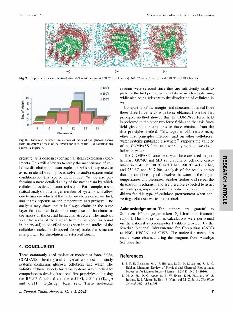
RESEARCH

ARTIC

LE

Bazooyar et al. Molecular Modelling of Cellulose Dissolution

(a) (b) (c)

Fig. 7. Typical snap shots obtained after NpT equilibration at 100 �C and 1 bar (a), 160 �C and 6.2 bar (b) and 250 �C and 39.7 bar (c).

Fig. 8. Distances between the centres of mass of the glucose chainsfrom the centre of mass of the crystal for each of the T –p combinationsshown in Figure 7.

pressure, as is done in experimental steam explosion exper-iments. This will allow us to study the mechanisms of cel-lulose dissolution in steam explosion which is expected toassist in identifying improved solvents and/or experimentalconditions for this type of pretreatment. We are also per-forming a more detailed study of the mechanism by whichcellulose dissolves in saturated steam. For example, a sta-tistical analysis of a larger number of systems will allowone to analyse which of the cellulose chains dissolves first,and if this depends on the temperature and pressure. Theanalysis may show that it is always chains in the outerlayer that dissolve first, but it may also be the chains atthe apices of the crystal hexagonal structure. The analysiswill also reveal if the change from an in-plane (as foundin the crystal) to out-of-plane (as seen in the studies of thecellobiose molecule discussed above) molecular structureis important for dissolution in saturated steam.

4. CONCLUSION

Three commonly used molecular mechanics force fields,COMPASS, Dreiding and Universal were used to studysystems containing glucose, cellobiose and water. Thevalidity of these models for these systems was checked bycomparison to density functional first principles data usingthe B3LYP functional and the 6-311G, 6-311++G(d,p)and 6-311++G(2d, 2p) basis sets. These molecular

systems were selected since they are sufficiently small toperform the first principles calculations in a tractable time,while also being relevant to the dissolution of cellulose inwater.Comparison of the energies and structures obtained from

these three force fields with those obtained from the firstprinciples method showed that the COMPASS force fieldis preferred to the other two force fields and that this forcefield gives similar structures to those obtained from thefirst principles method. This, together with results usingother first principles methods and on other cellobiose-water systems published elsewhere32 supports the validityof the COMPASS force field for studying cellulose disso-lution in water.The COMPASS force field was therefore used in pre-

liminary GCMC and MD simulations of cellulose disso-lution in water at 100 �C and 1 bar, 160 �C and 6.2 bar,and 250 �C and 39.7 bar. Analysis of the results showsthat the cellulose crystal dissolves in water at the highertemperatures and pressures. Further studies will reveal thedissolution mechanism and are therefore expected to assistin identifying improved solvents and/or experimental con-ditions for this type of cellulose pretreatment when con-verting cellulosic waste into biofuel.

Acknowledgments: The authors are grateful toStiftelsen Föreningssparbanken Sjuhärad for financialsupport. The first principles calculations were performedon the national supercomputer facilities provided by theSwedish National Infrastructure for Computing (SNIC)at NSC, HPC2N and C3SE. The molecular mechanicsresults were obtained using the program from AccelrysSoftware Inc.

References

1. P. F. H. Harmsen, W. J. J. Huijgen, L. M. B. López, and R. R. C.Bakker, Literature Review of Physical and Chemical PretreatmentProcesses for Lignocellulosic Biomass, ECN-E–10-013 (2010).

2. M. A. Ha, D. C. Apperley, B. W. Evans, I. M. Huxham, W. G.Jardine, R. J. Vietor, D. Reis, B. Vian, and M. C. Jarvis, The PlantJournal 16:2, 183 (1998).

J. Comput. Theor. Nanosci. 10, 1–8, 2013 7

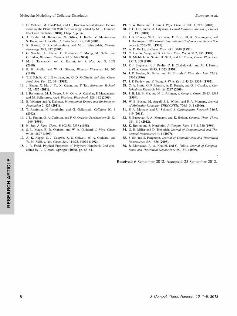
RESEARCH

ARTIC

LE

Molecular Modelling of Cellulose Dissolution Bazooyar et al.

3. D. Mohnen, M. Bar-Peled, and C., Biomass Recalcitrance: Decon-structing the Plant Cell Wall for Bioenergy, edited by M. E. Himmel,Blackwell Publisher (2008), Chap. 5, p. 96.

4. A. Berlin, M. Balakshin, N. Gilkes, J. Kadla, V. Maximenko,S. Kubo, and J. Saddler, J. Biotechnol. 125, 198 (2006).

5. K. Karimi, S. Kheradmandinia, and M. J. Taherzadeh, BiomassBioenergy 30:3, 247 (2006).

6. G. Sanchez, L. Pilcher, C. Roslander, T. Modig, M. Galbe, andG. Liden, Bioresour. Technol. 93:3, 249 (2004).

7. M. J. Taherzadeh and K. Karimi, Int. J. Mol. Sci. 9, 1621(2008).

8. B. K. Avellar and W. G. Glasser, Biomass Bioenergy 14, 205(1998).

9. T. P. Schultz, C. J. Biermann, and G. D. McGinnis, Ind. Eng. Chem.Prod. Res. Dev. 22, 344 (1983).

10. J. Zhang, X. Ma, J. Yu, X. Zhang, and T. Tan, Bioresour. Technol.102, 4585 (2011).

11. I. Ballesteros, M. J. Negro, J. M. Oliva, A. Cabañas, P. Manzanares,and M. Ballesteros, Appl. Biochem. Biotechnol. 129–132 (2006).

12. B. Volynets and Y. Dahman, International Energy and EnvironmentFoundation 2, 427 (2011).

13. T. Josefsson, H. Lennholm, and G. Gellerstedt, Cellulose 00, 1(2002).

14. J. L. Faulon, G. A. Carlsson, and P. G. Organic Geochemistry 21:12,1169 (1994).

15. H. Sun, J. Phys. Chem., B 102:38, 7338 (1998).16. S. L. Mayo, B. D. Olafson, and W. A. Goddard, J. Phys. Chem.

94:26, 8897 (1990).17. A. K. Rappe, C. J. Casewit, K. S. Colwell, W. A. Goddard, and

W. M. Skiff, J. Am. Chem. Soc. 114:25, 10024 (1992).18. J. R. Freid, Physical Properties of Polymers Handbook, 2nd edn.,

edited by A. E. Mark, Springer (2006), pp. 63–64.

19. S. W. Bunte and H. Sun, J. Phys. Chem. B 104:11, 2477 (2000).20. T. C. Lim, and R. A. Udyavara, Central European Journal of Physics

7:1, 193 (2009).21. J. S. Conery, W. L. Peticolas, T. Rush, III, K. Shanmugam, and

J. Dominguez, 28th Hawaii International Conference on System Sci-ences �HICSS’95� (1995).

22. A. D. Becke, J. Chem. Phys. 98:7, 5648 (1993).23. C. Lee, W. Yang, and R. G. Parr, Phys. Rev. B 37:2, 785 (1988).24. B. Miehlich, A. Savin, H. Stoll, and H. Preuss, Chem. Phys. Lett.

157:3, 200 (1989).25. P. J. Stephens, F. J. Devlin, C. F. Chabalowski, and M. J. Frisch,

J. Phys. Chem. 98:45, 11623 (1994).26. J. P. Perdew, K. Burke, and M. Ernzerhof, Phys. Rev. Lett. 77:18,

3865 (1996).27. J. P. Perdew and Y. Wang, J. Phys. Rev. B 45:23, 13244 (1992).28. C. A. Stortz, G. P. Johnson, A. D. French, and G. I. Csonka, J. Car-

bohydrate Research 344:16, 2217 (2009).29. J. H. Lii, B. Ma, and N. L. Allinger, J. Comput. Chem. 20:15, 1593

(1999).30. W. B. Bosma, M. Appell, J. L. Willett, and F. A. Momany, Journal

of Molecular Structure: THEOCHEM. 776:1–3, 1 (2006).31. F. A. Momany and U. Schnupf, J. Carbohydrate Research 346:5,

619 (2011).32. F. Bazooyar, F. A. Momany, and K. Bolton, Comput. Theo. Chem.

984, 119 (2012).33. K. Bolton and S. Nordholm, J. Comput. Phys. 113:2, 320 (1994).34. G. H. Miller and D. Trebotich, Journal of Computational and The-

oretical Nanoscience 4, 1 (2007).35. S Bin and S. Fanghong, Journal of Computational and Theoretical

Nanoscience 5:8, 1556 (2008).36. B. Mortazavi, A. A. Khatibi, and C. Politis, Journal of Computa-

tional and Theoretical Nanoscience 6:3, 644 (2009).

Received: 6 September 2012. Accepted: 25 September 2012.

.

8 J. Comput. Theor. Nanosci. 10, 1–8, 2013

Paper III

1

Molecular-level Simulations of Cellulose Steam Explosion

Faranak Bazooyar1, 2 and Kim Bolton1, *

1 School of Engineering, University of Borås, Borås, SE-501 90, Sweden

2 Department of Chemical Engineering, Chalmers University of Technology, Gothenburg, SE-

412 96, Sweden

*Corresponding author: Kim Bolton (E-mail: kim.bolton@hb.se) -School of Engineering, University of Borås, SE-501 90, Borås, Sweden, Tel: +46 33 435 4602

ABSTRACT

Grand canonical Monte Carlo and molecular dynamics simulations are used to study steam

explosion of crystalline cellulose using 100, 160, 210 and 250 °C saturated steam. The

simulations are based on the COMPASS force field, which provides a valid description of the

cellulose crystal structure and water-cellobiose interactions. Disruption of the crystal

structure during steaming is typically larger than that during the explosion stage and the

restructuring is larger at increased temperature and pressure. This is seen by an increased

separation of the cellulose chains from the center of mass of the crystal during the initial

stages of the steaming, especially for chains in the outer shell of the elementary fibril. There

is a large change in the radius of gyration and fraction of anti torsion angle conformers for

chains in the outer shell of the elementary fibril. In addition, the disruption at the reducing

and non-reducing ends of the cellulose crystal is larger than in the central core, increasing

susceptibility to enzymatic attack in these end regions.

Keywords: cellulose, molecular dynamics, Monte Carlo, steam explosion

2

1. INTRODUCTION

A large amount of research has focused on lignocellulosic material as a source for fuel since it is the

most abundant organic material in the biosphere.1 However, the complex molecular structure of this

material makes it difficult to decompose it to the smaller molecules needed for biological conversion

to fuels such as ethanol and methane. A variety of pretreatment methods have therefore been used

to increase the accessibility of cellulose to enzymatic and chemical hydrolysis.2 One such method is

steam explosion, which is an effective and inexpensive method that has lower environmental impact

and fewer hazardous products than many of the other methods.3, 4 It was developed by Mason 5 in

1925 and used by Babcock 6 in 1932 as a pretreatment method for bioethanol production.

Experimental investigations of steam explosion have studied the effect of temperature,

pressure and residence time when pretreating feedstocks such as wheat straw, sweet

sorghum, aspen wood and hardwood chips.2, 7-14 The method consists of two stages. In the

steaming stage the material is subjected to high pressure saturated steam and in the second

stage, known as explosion, there is a rapid pressure drop to atmospheric pressure. Steam

explosion helps to remove, depolymerise and dissolve lignin and hemicellulose into lower

molecular-weight products, and it also reduces the size and crystallinity of the cellulose

structure.10 It is believed that the crystalline structure becomes disordered, which increases

the surface area and enhances the accessibility to enzymes, hence leading to more efficient

hydrolysis.8, 9, 11, 13 Typically, an increase in temperature, pressure and/or residence time

increases the disruption of the cellulose structure.14, 15 Steam explosion is the most effective

pretreatment method in commercial production of bioethanol from feedstock such as wheat

straw.16

Computational methods have been used to study a wide range of materials and chemical

processes.17-25 They complement experimental research since they offer easy manipulation

3

and analysis at the molecular level, which is often difficult to obtain from experiment. This

leads to a molecular level understanding of chemical processes, which can be combined with

knowledge obtained from experiments to improve existing, and identify novel, processing

techniques. Examples include studies of the structure26 and of the thermal behavior of

cellulose.27, 28 These studies provide molecular-level insight of some structural changes, such

as expansion of the cellulose crystal, with increasing temperature. Although there exist

numerous studies of structures that are relevant to cellulose, such as cellobiose,29- 33 apart

from the preliminary studies presented by us 34 there have been no molecular level studies

of cellulose steam explosion. This contribution presents results obtained from a combined

Monte Carlo (MC) and molecular dynamics (MD) study of the steaming and explosion

processes, thereby yielding a molecular level understanding of the changes in the cellulose

crystal structure during these processes. The (temperature, pressure) combinations that

were studied are (100 °C, 1.0 bar), (160 °C, 6.2 bar), (210 °C, 19.0 bar) and (250 °C, 39.7 bar).

The last three combinations have been used in experimental studies of steam explosion,8, 2,

35 and the first combination is studied as a reference system to ensure that the simulations

have equilibrated in the steaming and explosion stages.

The studies presented here are for a crystalline cellulose structure, since dissolving and

decomposing this ordered structure is believed to be the bottleneck for biological

conversion of lignocellulosic materials to fuel.36 Although the compositions and structures of

different lignocellulosic materials can vary, they typically consist of cellulose elementary

fibrils that are covered with lignin and hemicellulose. The elementary fibril is crystalline and

is composed of linear polymer chains consisting of β-(1, 4)-D-glucan units. Different

structures of the elementary fibrils have been suggested for different plant cell walls,37- 40

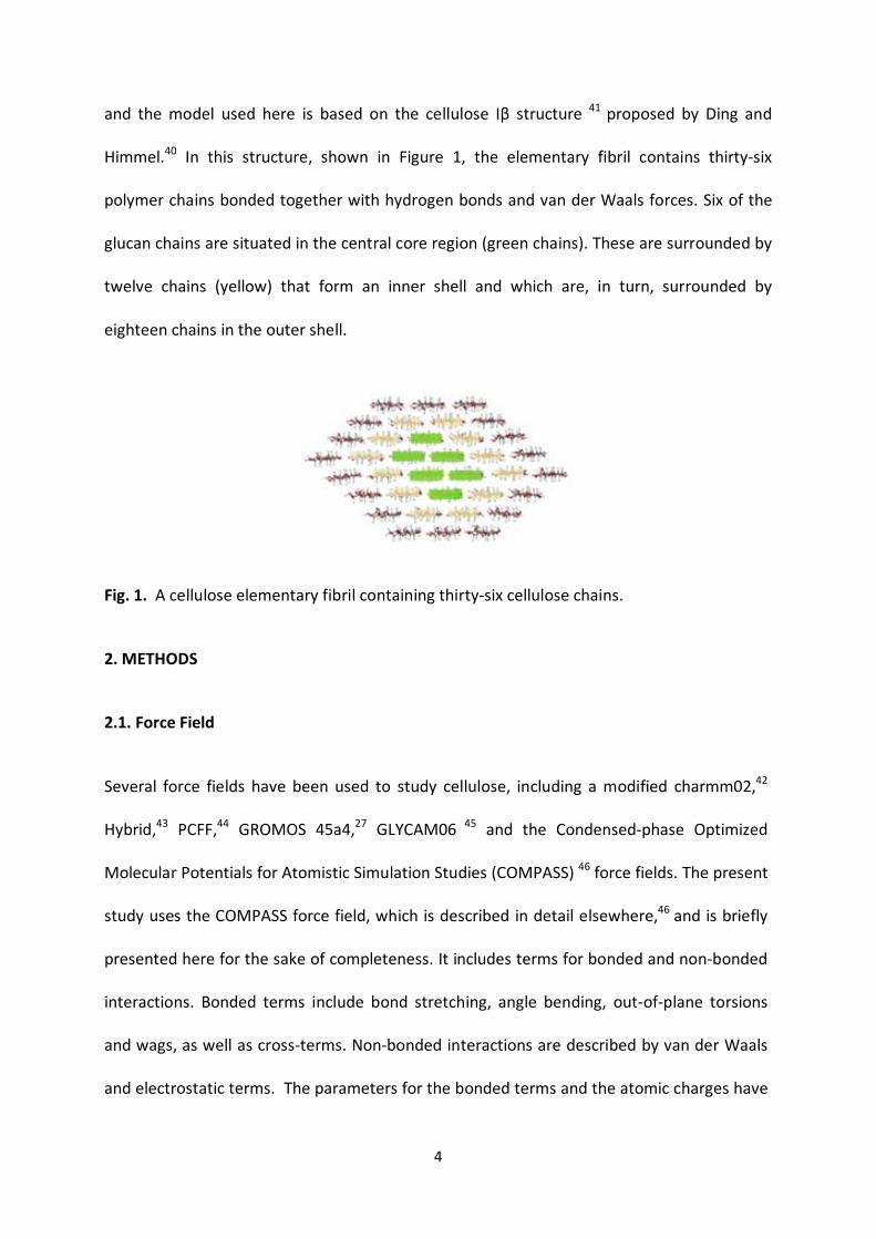
4

and the model used here is based on the cellulose Iβ structure 41 proposed by Ding and

Himmel.40 In this structure, shown in Figure 1, the elementary fibril contains thirty-six

polymer chains bonded together with hydrogen bonds and van der Waals forces. Six of the

glucan chains are situated in the central core region (green chains). These are surrounded by

twelve chains (yellow) that form an inner shell and which are, in turn, surrounded by

eighteen chains in the outer shell.

Fig. 1. A cellulose elementary fibril containing thirty-six cellulose chains.

2. METHODS

2.1. Force Field

Several force fields have been used to study cellulose, including a modified charmm02,42

Hybrid,43 PCFF,44 GROMOS 45a4,27 GLYCAM06 45 and the Condensed-phase Optimized

Molecular Potentials for Atomistic Simulation Studies (COMPASS) 46 force fields. The present

study uses the COMPASS force field, which is described in detail elsewhere,46 and is briefly

presented here for the sake of completeness. It includes terms for bonded and non-bonded

interactions. Bonded terms include bond stretching, angle bending, out-of-plane torsions

and wags, as well as cross-terms. Non-bonded interactions are described by van der Waals

and electrostatic terms. The parameters for the bonded terms and the atomic charges have

5

been fit to ab initio data and those for the non-bonded terms are fit to experiment.46 The fit

has been made to a variety of materials including polymers.47

Studies by Aldred 48 revealed that the COMPASS force field yields valid structures for

cellulose crystal systems, similar to those studied here. He combined this force field with

canonical (NVT) MD simulations and geometry optimizations to obtain a unit cell structure

for the Iβ polymorph (also studied in this work) with a= 7.44 Å, b=8.02 Å, c= 10.42 Å and γ=

98.33° (these cell parameters are shown in Figure 2). This differs by 5.2, 3.0, 0.4 and 2.1%

from the crystal structure based on X-ray diffraction data obtained by Sarko and Muggli,49

which has values of a= 7.85 Å, b=8.27 Å, c= 10.38 Å and γ= 96.3°. Aldred 48 also showed that

the COMPASS force field yields valid structures of the II polymorph. Miyamoto et al.50 has

also shown that this force field provides a valid structure for cellulose II, and they have also

used this force field to study cellulose Iβ.51 Eichhorn and Davies 52 used this force field to

compare the mechanical properties of cellulose I and II, and studies by Wu and co-workers 53

showed that the COMPASS force field yields elastic properties of cellulose nanocrystals that

are in agreement with experimental data and other MD simulations. They also used the

COMPASS force field to calculate the elasticity of single cellulose chains.54 Hence, previous

studies show that the COMPASS force field yields valid structures and mechanical properties

of cellulose crystal structures.

This previous work has been extended by us to study unit cell parameters and densities of

the crystalline cellulose structure based on Ding and Himmel’s model.40 This structure was

equilibrated at 25 and 250 °C, since there are experimental data at these temperatures and

the lower temperature is room temperature and the higher temperature is just below the

cellulose melting point. The unit cell parameters are a= 7.85 Å, b=8.32 Å, c= 10.50 Å and γ=

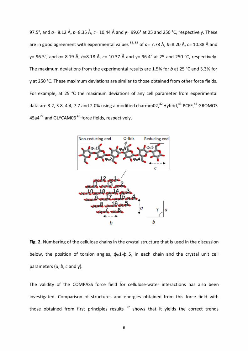
6

97.5°, and a= 8.12 Å, b=8.35 Å, c= 10.44 Å and γ= 99.6° at 25 and 250 °C, respectively. These

are in good agreement with experimental values 55, 56 of a= 7.78 Å, b=8.20 Å, c= 10.38 Å and

γ= 96.5°, and a= 8.19 Å, b=8.18 Å, c= 10.37 Å and γ= 96.4° at 25 and 250 °C, respectively.

The maximum deviations from the experimental results are 1.5% for b at 25 °C and 3.3% for

γ at 250 °C. These maximum deviations are similar to those obtained from other force fields.

For example, at 25 °C the maximum deviations of any cell parameter from experimental

data are 3.2, 3.8, 4.4, 7.7 and 2.0% using a modified charmm02,42 Hybrid,43 PCFF,44 GROMOS

45a4 27 and GLYCAM06 45 force fields, respectively.

Fig. 2. Numbering of the cellulose chains in the crystal structure that is used in the discussion

below, the position of torsion angles, φH1-φH5, in each chain and the crystal unit cell

parameters (a, b, c and γ).

The validity of the COMPASS force field for cellulose-water interactions has also been

investigated. Comparison of structures and energies obtained from this force field with

those obtained from first principles results 57 shows that it yields the correct trends

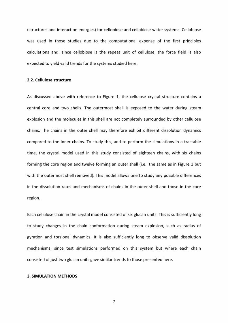
7

(structures and interaction energies) for cellobiose and cellobiose-water systems. Cellobiose

was used in those studies due to the computational expense of the first principles

calculations and, since cellobiose is the repeat unit of cellulose, the force field is also

expected to yield valid trends for the systems studied here.

2.2. Cellulose structure

As discussed above with reference to Figure 1, the cellulose crystal structure contains a

central core and two shells. The outermost shell is exposed to the water during steam

explosion and the molecules in this shell are not completely surrounded by other cellulose

chains. The chains in the outer shell may therefore exhibit different dissolution dynamics

compared to the inner chains. To study this, and to perform the simulations in a tractable

time, the crystal model used in this study consisted of eighteen chains, with six chains

forming the core region and twelve forming an outer shell (i.e., the same as in Figure 1 but

with the outermost shell removed). This model allows one to study any possible differences

in the dissolution rates and mechanisms of chains in the outer shell and those in the core

region.

Each cellulose chain in the crystal model consisted of six glucan units. This is sufficiently long

to study changes in the chain conformation during steam explosion, such as radius of

gyration and torsional dynamics. It is also sufficiently long to observe valid dissolution

mechanisms, since test simulations performed on this system but where each chain

consisted of just two glucan units gave similar trends to those presented here.

3. SIMULATION METHODS

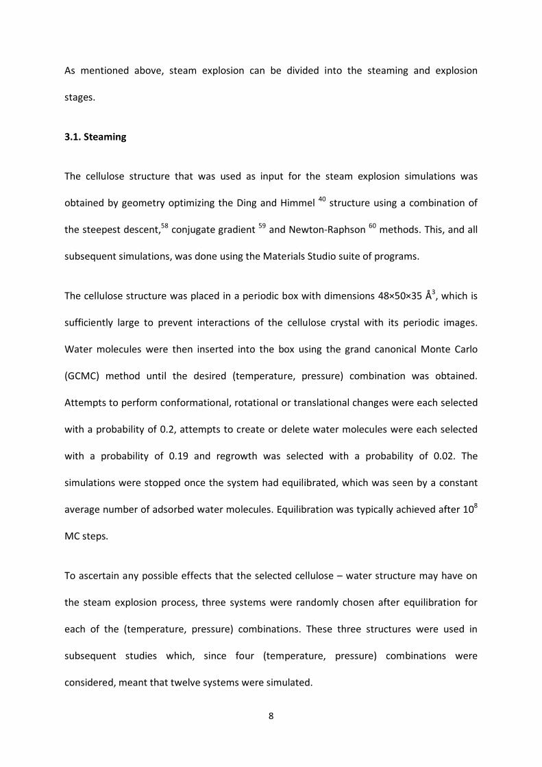
8

As mentioned above, steam explosion can be divided into the steaming and explosion

stages.

3.1. Steaming

The cellulose structure that was used as input for the steam explosion simulations was

obtained by geometry optimizing the Ding and Himmel 40 structure using a combination of

the steepest descent,58 conjugate gradient 59 and Newton-Raphson 60 methods. This, and all

subsequent simulations, was done using the Materials Studio suite of programs.

The cellulose structure was placed in a periodic box with dimensions 48×50×35 Å3, which is

sufficiently large to prevent interactions of the cellulose crystal with its periodic images.

Water molecules were then inserted into the box using the grand canonical Monte Carlo

(GCMC) method until the desired (temperature, pressure) combination was obtained.

Attempts to perform conformational, rotational or translational changes were each selected

with a probability of 0.2, attempts to create or delete water molecules were each selected

with a probability of 0.19 and regrowth was selected with a probability of 0.02. The

simulations were stopped once the system had equilibrated, which was seen by a constant

average number of adsorbed water molecules. Equilibration was typically achieved after 108

MC steps.

To ascertain any possible effects that the selected cellulose – water structure may have on

the steam explosion process, three systems were randomly chosen after equilibration for

each of the (temperature, pressure) combinations. These three structures were used in

subsequent studies which, since four (temperature, pressure) combinations were

considered, meant that twelve systems were simulated.

9

Since the Materials Studio program does not allow for relaxation of the cellulose chains

during GCMC, the structures were further simulated using canonical (NVT) MD at the same

temperature and volume used in the GCMC simulations. The MD trajectories were typically

propagated for 300 ps using a time-step of 1 fs. This is sufficiently long to obtain

equilibrated structures, as seen from the constant average values of the data presented

below. Integration was performed using the Verlet algorithm, which has the strength of

being time-reversible.61 The temperature of the system was controlled using the Nose

thermostat.62- 64 An equilibrated structure obtained from this simulation was used as input

for a second GCMC equilibration simulation. The effect of the MD simulation on the

number of absorbed water molecules proved to be very small with less than 0.5% of water

being adsorbed in the second simulation compared to the first GCMC simulation. The

process was repeated, and the configuration obtained at the end of the second MD

simulation showed no tendency to absorb more water in the subsequent GCMC simulation.

3.2. Explosion

The twelve structures obtained from the steaming simulations were used as input for the

explosion simulations. These were performed using MD in the isobaric-isothermal (NpT)

ensemble using the same temperature as in the steaming simulations but at a pressure of 1

bar. The trajectories were typically propagated for 300 ps using a time-step of 1 fs (as

discussed below, this is sufficiently long to obtain convergence and hence longer

trajectories are not required). The temperature was controlled using the Nose thermostat,

62- 64 while the pressure was controlled by the Berendsen barostat.65

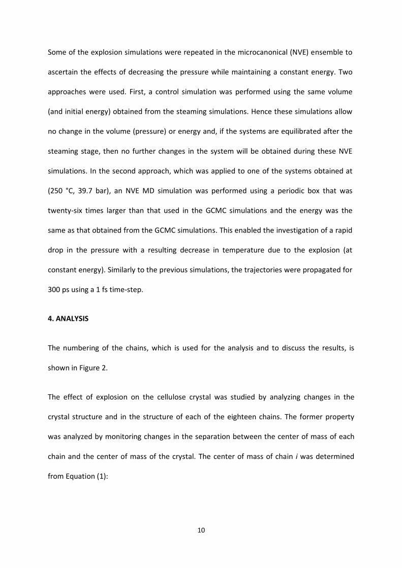
10

Some of the explosion simulations were repeated in the microcanonical (NVE) ensemble to

ascertain the effects of decreasing the pressure while maintaining a constant energy. Two

approaches were used. First, a control simulation was performed using the same volume

(and initial energy) obtained from the steaming simulations. Hence these simulations allow

no change in the volume (pressure) or energy and, if the systems are equilibrated after the

steaming stage, then no further changes in the system will be obtained during these NVE

simulations. In the second approach, which was applied to one of the systems obtained at

(250 °C, 39.7 bar), an NVE MD simulation was performed using a periodic box that was

twenty-six times larger than that used in the GCMC simulations and the energy was the

same as that obtained from the GCMC simulations. This enabled the investigation of a rapid

drop in the pressure with a resulting decrease in temperature due to the explosion (at

constant energy). Similarly to the previous simulations, the trajectories were propagated for

300 ps using a 1 fs time-step.

4. ANALYSIS

The numbering of the chains, which is used for the analysis and to discuss the results, is

shown in Figure 2.

The effect of explosion on the cellulose crystal was studied by analyzing changes in the

crystal structure and in the structure of each of the eighteen chains. The former property

was analyzed by monitoring changes in the separation between the center of mass of each

chain and the center of mass of the crystal. The center of mass of chain i was determined

from Equation (1):

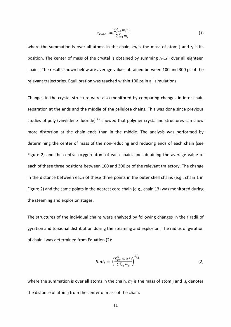
11

𝑟𝐶𝑜𝑀,𝑖 =∑ 𝑚𝑗𝑟𝑗𝑁𝑗=1

∑ 𝑚𝑗𝑁𝑗=1

(1)

where the summation is over all atoms in the chain, mj is the mass of atom j and rj is its

position. The center of mass of the crystal is obtained by summing rCoM, i over all eighteen

chains. The results shown below are average values obtained between 100 and 300 ps of the

relevant trajectories. Equilibration was reached within 100 ps in all simulations.

Changes in the crystal structure were also monitored by comparing changes in inter-chain

separation at the ends and the middle of the cellulose chains. This was done since previous

studies of poly (vinylidene fluoride) 66 showed that polymer crystalline structures can show

more distortion at the chain ends than in the middle. The analysis was performed by

determining the center of mass of the non-reducing and reducing ends of each chain (see

Figure 2) and the central oxygen atom of each chain, and obtaining the average value of

each of these three positions between 100 and 300 ps of the relevant trajectory. The change

in the distance between each of these three points in the outer shell chains (e.g., chain 1 in

Figure 2) and the same points in the nearest core chain (e.g., chain 13) was monitored during

the steaming and explosion stages.

The structures of the individual chains were analyzed by following changes in their radii of

gyration and torsional distribution during the steaming and explosion. The radius of gyration

of chain i was determined from Equation (2):

𝑅𝑜𝐺𝑖 = �∑ 𝑚𝑗𝑠2𝑗𝑁𝑗=1∑ 𝑚𝑗𝑁𝑗=1

�12�

(2)

where the summation is over all atoms in the chain, mj is the mass of atom j and sj denotes

the distance of atom j from the center of mass of the chain.

12

Figure 2 shows the positions of the five torsion angles, φH1 to φH5,47, 67 that were monitored

during the steaming and explosion. The numbering of each cellobiose unit and φH are the

same as in reference 58, where φH= H-1-C-1-O-C-4´ for each cellobiose unit. Analysis of the

torsion angles reveals possible changes in the population of syn and anti conformers during

the explosion. Our previous study 47 of cellobiose in bulk water showed that, due to the

presence of the water and to entropic effects at elevated temperatures, the syn conformer

67 is preferred. The present study will reveal if similar preferences for the syn conformers are

found for chains in the cellulose crystal under conditions relevant to steam explosion.

5. RESULTS AND DISCUSSION

Figure 3 illustrates the change in the crystal structure after steam explosion at 250 °C and

39.7 bar. These changes are quantified below.

13

Fig. 3. Illustration of the changes in the cellulose crystal structure during steam explosion at

250 °C and 39.7 bar.

5.1. Center of mass

Figure 4 shows the change in the separation of the center of mass of each chain from the

center of mass of the crystal due to the steaming process. Only the chains in the outer shell

are shown for the sake of clarity. The centers of mass at the beginning of the steaming are

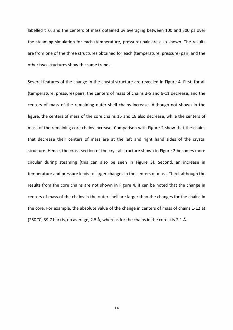
14

labelled t=0, and the centers of mass obtained by averaging between 100 and 300 ps over

the steaming simulation for each (temperature, pressure) pair are also shown. The results

are from one of the three structures obtained for each (temperature, pressure) pair, and the

other two structures show the same trends.

Several features of the change in the crystal structure are revealed in Figure 4. First, for all

(temperature, pressure) pairs, the centers of mass of chains 3-5 and 9-11 decrease, and the

centers of mass of the remaining outer shell chains increase. Although not shown in the

figure, the centers of mass of the core chains 15 and 18 also decrease, while the centers of

mass of the remaining core chains increase. Comparison with Figure 2 show that the chains

that decrease their centers of mass are at the left and right hand sides of the crystal

structure. Hence, the cross-section of the crystal structure shown in Figure 2 becomes more

circular during steaming (this can also be seen in Figure 3). Second, an increase in

temperature and pressure leads to larger changes in the centers of mass. Third, although the

results from the core chains are not shown in Figure 4, it can be noted that the change in

centers of mass of the chains in the outer shell are larger than the changes for the chains in

the core. For example, the absolute value of the change in centers of mass of chains 1-12 at

(250 °C, 39.7 bar) is, on average, 2.5 Å, whereas for the chains in the core it is 2.1 Å.

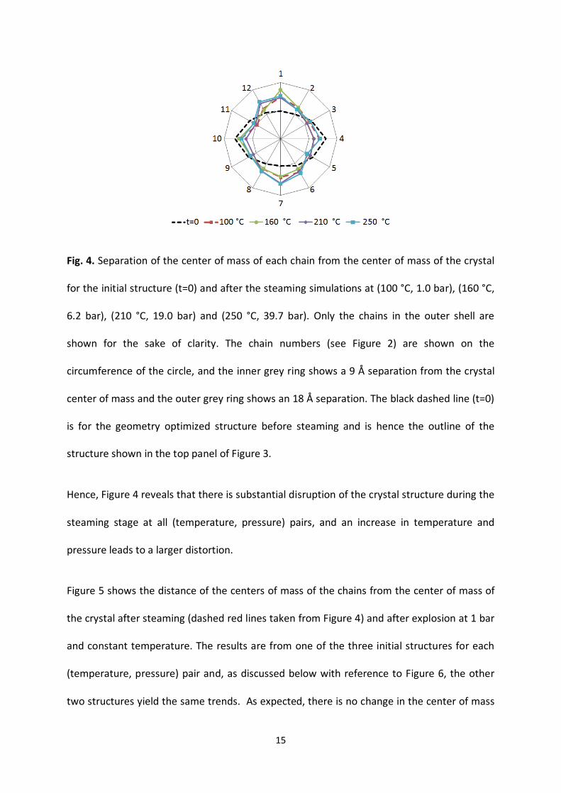
15

Fig. 4. Separation of the center of mass of each chain from the center of mass of the crystal

for the initial structure (t=0) and after the steaming simulations at (100 °C, 1.0 bar), (160 °C,

6.2 bar), (210 °C, 19.0 bar) and (250 °C, 39.7 bar). Only the chains in the outer shell are

shown for the sake of clarity. The chain numbers (see Figure 2) are shown on the

circumference of the circle, and the inner grey ring shows a 9 Å separation from the crystal

center of mass and the outer grey ring shows an 18 Å separation. The black dashed line (t=0)

is for the geometry optimized structure before steaming and is hence the outline of the

structure shown in the top panel of Figure 3.

Hence, Figure 4 reveals that there is substantial disruption of the crystal structure during the

steaming stage at all (temperature, pressure) pairs, and an increase in temperature and

pressure leads to a larger distortion.

Figure 5 shows the distance of the centers of mass of the chains from the center of mass of

the crystal after steaming (dashed red lines taken from Figure 4) and after explosion at 1 bar

and constant temperature. The results are from one of the three initial structures for each

(temperature, pressure) pair and, as discussed below with reference to Figure 6, the other

two structures yield the same trends. As expected, there is no change in the center of mass

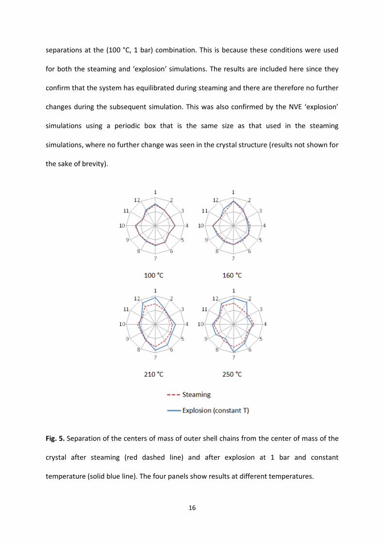
16

separations at the (100 °C, 1 bar) combination. This is because these conditions were used

for both the steaming and ‘explosion’ simulations. The results are included here since they

confirm that the system has equilibrated during steaming and there are therefore no further

changes during the subsequent simulation. This was also confirmed by the NVE ‘explosion’

simulations using a periodic box that is the same size as that used in the steaming

simulations, where no further change was seen in the crystal structure (results not shown for

the sake of brevity).

Fig. 5. Separation of the centers of mass of outer shell chains from the center of mass of the

crystal after steaming (red dashed line) and after explosion at 1 bar and constant

temperature (solid blue line). The four panels show results at different temperatures.

17

Figure 5 shows that, similar to the change in the crystal structure during steaming, an

increase in temperature and pressure leads to a larger disruption of the cellulose crystal

structure during explosion. Also, although not shown in the figure (for the sake of clarity),

the change in center of mass separation is largest for the chains in the outer shell compared

to those in the core region. That is, the central cellulose chains (13-18) show very small

changes compared to many of the chains in the outer shell (1-12). For example, the absolute

value of the change in centers of mass of chains 1-12 during the explosion stage at (250 °C,

39.7 bar) is, on average, 1.9 Å, whereas for the chains in the core it is 0.8 Å.

Figure 6 shows the same information shown in Figure 5 but for all three initial structures at

(250 °C, 39.7 bar). It is clear that the trends discussed above are observed for all structures,

and the results are therefore not sensitive to the initial structure of the cellulose after

steaming. These results, as well as those shown in Figure 5, also show that any of the outer

chains may show the largest change in center of mass during steaming and explosion. That

is, although the chains in the outer shell show a larger change in center of mass than the

core chains, there is no preference as to which of chains 1-12 show the largest changes

during steam explosion. In contrast, a large change in center of mass of a core chain requires

that the neighboring chains in the outer shell also have a large change in their centers of

mass. For example, the simulations showed that a large change in the center of mass of

chain 13 requires large changes in its neighboring chains 1 and 12 (see Figure 2).

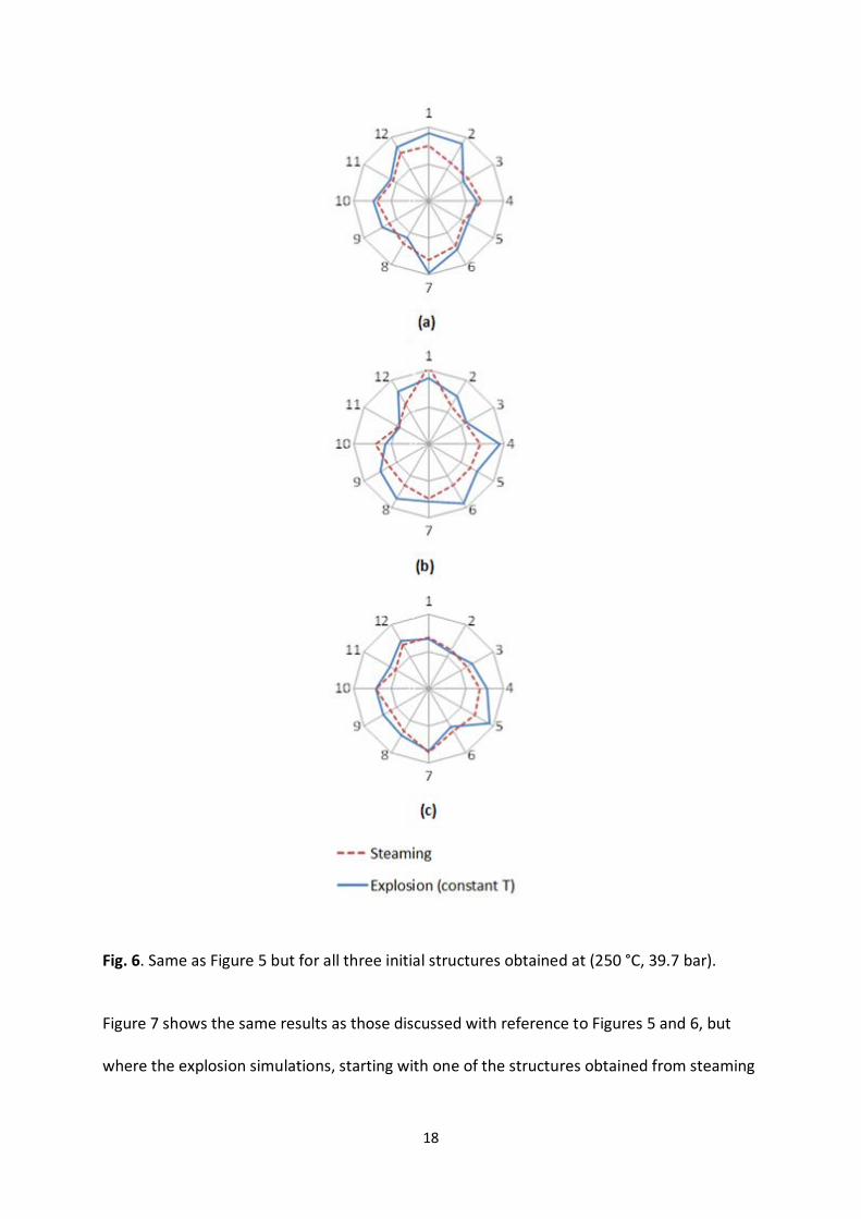
18

Fig. 6. Same as Figure 5 but for all three initial structures obtained at (250 °C, 39.7 bar).

Figure 7 shows the same results as those discussed with reference to Figures 5 and 6, but

where the explosion simulations, starting with one of the structures obtained from steaming

19

at (250 °C, 39.7 bar), are performed using NVE molecular dynamics with a volume 26 times

larger than that used for steaming. Hence, the pressure on the cellulose-water system is zero

(water molecules do not leave and re-enter the periodic box during the simulation) and the

energy is constant. Due to the explosion at constant energy, the temperature decreases by

80 °C.

Fig. 7. Same as Figure 5 but using NVE with the large box to simulate the explosion stage.

Figure 7 shows that there is very little change in the centers of mass of the chains when

performing the explosion simulations under constant energy conditions. Hence, it is the

constant temperature, and not the drop in pressure, than caused the change in centers of

mass during the NpT simulations. Since experimental explosion is performed under NVE

conditions (but where the final pressure is 1 bar), the results obtained here indicate that

most of the disruption of the crystal structure occurs during the steaming stage.

Analysis of the center of mass separations during steaming shows that the largest changes

occur during the first 4 ps, and at longer times the distance between center of mass of each

20

chain and the crystal fluctuate around a constant value. This reveals that the disruption

occurs during the very early stages of the steaming process.

Additional insight of steaming on the disruption of the cellulose crystal structure was

obtained from the inter- and intra-chain van der Waals energies. Under all conditions

studied (and for all three initial structures) there is an increase in both inter- and intra-chain

energies during the steaming process. This is expected, at least for the inter-chain energies,

since disruption of the crystal structure results in larger inter-chain separations and hence

higher van der Waals energies. For example, at 250 °C the inter-chain van der Waals energy

increased by about 1025 kcal/mol during the steaming process. The increase in the intra-

chain van der Waals energy is small compared to the increase in inter-chain energy.

There is no significant correlation between the magnitude of the change in centers of mass

of chains during steaming and explosion and changes in their radii of gyration. As an

example, Figure 8 shows the change in radius of gyration for each chain as a function of its

change in center of mass during explosion at 250 °C and 1 bar. The results are typical for all

initial structures and (temperature, pressure) pairs. The lines shown in the figure are best-fit

straight lines to the core chains (dashed line), the chains in the outer shell (thin solid line)

and all eighteen chains (thick solid line). Although all three curves show a trend of

decreasing change in radius of gyration with increasing change in center of mass, there is a

large scattering (the R-squared values are 0.42, 0.24 and 0.27 for each of the fits,

respectively).

21

Fig. 8. Change in radius of gyration for each chain as a function of its change in center of

mass during explosion at 250 °C and 1 bar. The lines are best-fit straight lines to the core

chains (dashed line), the chains in the outer shell (thin solid line) and all eighteen chains

(thick solid line).

The left column of Figure 9 shows the change in separation between the non-reducing end

of a chain in the outer shell and the same end of the neighboring core chain. The central and

right columns show the change in separation between the central O-links between outer and

neighboring core chains, and the change in separation between the reducing ends of the

outer chains and their neighboring core chains. The results are for steaming at (250 °C, 39.7

bar) and for explosion at this temperature. The figure reveals that there is larger disruption

at the ends of the chains than at the middle during both steaming and explosion. It should

also be noted that the values in the figure are averages over all outer chains, and that some

chain ends are separated by as much as 16.1 Å from the neighboring inner chain ends.

Hence, after steaming and explosion the ends of the crystalline elementary fibrils are more

accessible to enzymatic attack than other regions of the fibril.

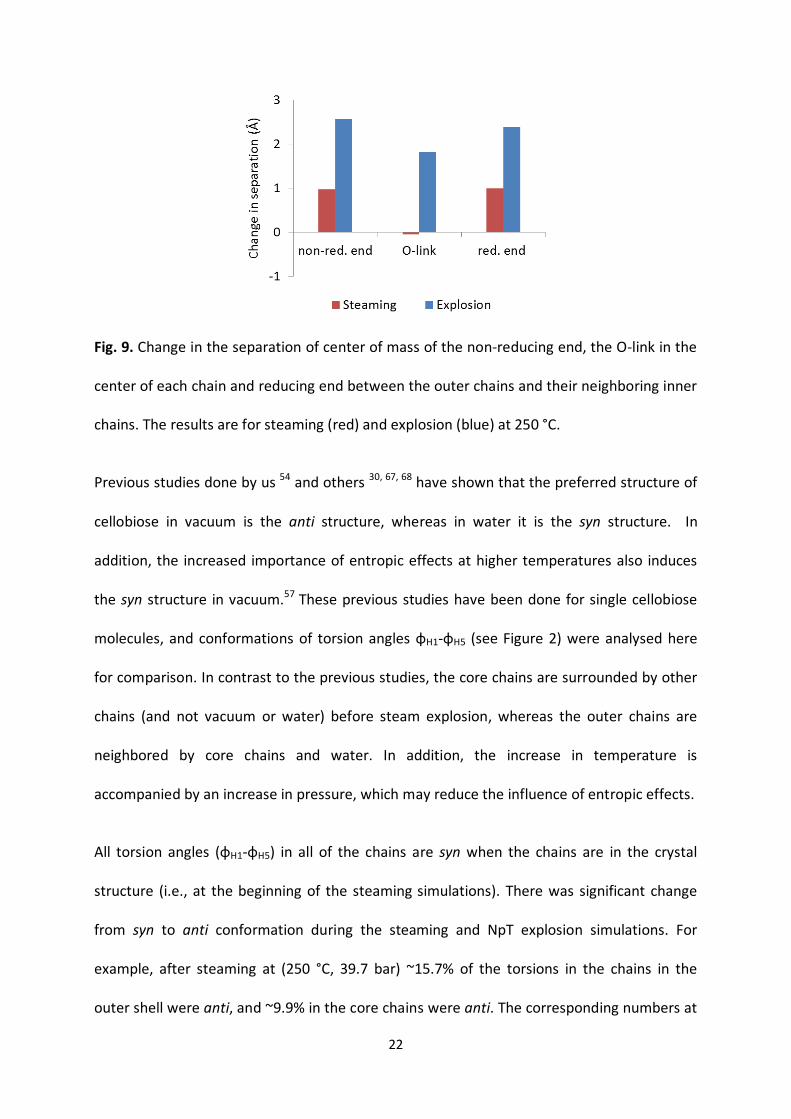
22

Fig. 9. Change in the separation of center of mass of the non-reducing end, the O-link in the

center of each chain and reducing end between the outer chains and their neighboring inner

chains. The results are for steaming (red) and explosion (blue) at 250 °C.

Previous studies done by us 54 and others 30, 67, 68 have shown that the preferred structure of

cellobiose in vacuum is the anti structure, whereas in water it is the syn structure. In

addition, the increased importance of entropic effects at higher temperatures also induces

the syn structure in vacuum.57 These previous studies have been done for single cellobiose

molecules, and conformations of torsion angles φH1-φH5 (see Figure 2) were analysed here

for comparison. In contrast to the previous studies, the core chains are surrounded by other

chains (and not vacuum or water) before steam explosion, whereas the outer chains are

neighbored by core chains and water. In addition, the increase in temperature is

accompanied by an increase in pressure, which may reduce the influence of entropic effects.

All torsion angles (φH1-φH5) in all of the chains are syn when the chains are in the crystal

structure (i.e., at the beginning of the steaming simulations). There was significant change

from syn to anti conformation during the steaming and NpT explosion simulations. For

example, after steaming at (250 °C, 39.7 bar) ~15.7% of the torsions in the chains in the

outer shell were anti, and ~9.9% in the core chains were anti. The corresponding numbers at

23

(160 °C, 6.2 bar) were ~17.1% and ~7.4%. Explosion at 250 °C resulted in a further increase

to ~21.4% for chains in the outer shell and ~14.4% in the core chains, whereas NpT explosion

at 160 °C did not lead to a large increase in the percent of anti torsions (~17.9% for chains in

the outer shell and ~9.1% in the core chains). These trends are typical for all structures and

temperatures, and show that the chains in the outer shell, which also showed the largest

change in center of mass motion, change more readily to anti torsions than the confined

chains in the core region. In addition, a larger percentage of torsions change to the anti

conformer at the higher temperatures and pressures. No correlation was observed between

the percent anti of each torsion (φH1- φH5) and its position in the chain (i.e., whether the

torsion was at one of the ends or in the middle of the chain). Also, similarly to the results

presented above for the radius of gyration, there is no significant correlation between the

changes in percent anti conformer in a chain with its change in center of mass.

6. CONCLUSION

Grand canonical Monte Carlo and molecular dynamics studies of steam explosion show that

there is significant disruption of the crystal structure during the steaming stage. The

restructuring of the cellulose crystal, which is seen by large changes in the centers of mass of

cellulose chains during steaming, increases with increased temperature and pressure.

Disruption was larger for the chains in the outer shell compared to the core chains. In

addition, there was larger disruption at the reducing and non-reducing ends of the crystal.

This increases the cellulose crystal’s accessibility to enzymes, particularly at the ends of the

elementary fibrils, which is important for the cellulose pretreatment in production of

biofuel.

24

Analysis of the changes in the radius of gyration and percent anti torsion angle conformers in

each chain showed that there was a larger change in these properties for chains in the outer

cellulose shell compared to the chains in the core region. However, comparison between

chains within either the outer shell or core region showed that there was no significant

correlation between these changes and the change in center of mass of the chains. These

observations are valid for both the steaming and explosion stages and for all conditions

studied.

7. ACKNOWLEDGEMENTS

The authors are grateful to Stiftelsen Föreningssparbanken Sjuhärad and the Carl Trygger

Foundation for Scientific Research for financial support. Molecular simulations were done

using the program from Accelrys Software Inc. F.B. thanks Mahdi Salimi and Dr. Edvin

Erdtman for their assistance.

25

References

1. P.F.H. Harmsen, W.J.J. Huijgen, L.M. Bermúdez López, and R.R.C. Bakker, ECN-E--10-013

(2010)

2. M. J. Taherzadeh and K. Karimi, Int. J. Mol. Sci. 9, 1621-1651 (2008)

3. B. K. Avellar and W. G. Glasser, Biomass Bioenerg. 14, 205–218 (1998)

4. H. Kahr, A. Jäger and C. Lanzerstorfer, in Bioethanol, M. A. P. Lima, Ed; InTech.; chapter

7, pp 153-172 (2012)

5. W. H. Mason, Process and apparatus for disintegration of wood and THB like field, U.S.

Patent 1578609, March 30 (1926).

6. L.W. Babcock, Method of producing fermentable sugars and alcohol from wood, U.S.

Patent 1855464, April 26 (1932).

7. H. Lennholm, T. Josefsson and G. Gellerstedt, Cellulose 8, 289-296 (2001)

8. I. Ballesteros, M. José Negro, J.M. Oliva, A. Cabañas, P. Manzanares and M. Ballesteros,

Appl. Biochem. Biotechnol. 1, 129–132 (2006)

9. T. P. Schultz, C. J. Biermann and G. D. McGinnis, Ind. Eng. Chem. Prod. Res. Dev. 22, 344–

348 (1983)

10. J. Zhang, X. Ma, J. Yu, X. Zhang and T. Tan, Bioresour Technol. 102, 4585-9 (2011)

11. L. A. Donaldson, K. K. Y. Wong and K. L. Mackie, Wood Sci. Technol. 22, 103-114 (1988)

12. Y. Dahman and B. Volynets, Int. J. Energy Environ. 2, 427-446 (2011)

13. O. J. Rojas, R. Martin-Sampedro, E. A. Capanema, I. Hoeger and J. C. Villar, J. Agric. Food

Chem. 59, 8761–8769 (2011)

14. H. Theliander, K. Jedvert, A. Saltberg and M. E. Lindström, Bioresources. 7, 2051-2074

(2012)

26

15. N. Chacha, K. Toven, G. Mtui, J. Katima and G. Mrema, Cellulose Chem. Technol. 45, 495-

501 (2011)

16. Y. Dahman and B. Volynets, Int. J. Energy Environ. 2, 427- 446 (2011)

17. A. M. Ilyin, Quantum Matter, 2, 205-208 (2013)

18. E. Tylianakis and G. E. Froudakis, J. Comput. Theor. Nanosci. 6, 335-348 (2009)

19. G. H. Cocoletzi and N.Takeuchi, Quantum Matter, 2, 382-387 (2013)

20. M. Bohlén, K. C. Satyanarayana and K. Bolton, J. Comput. Theor. Nanosci. 10, 1317-1325

(2013)

21. M. Hashemy and M. Monajjemi, Quantum Matter, 2, 214-218 (2013)

22. M. Ibrahim and H. Elhaes, Reviews in Theoretical Science, 1, 368-376 (2013)

23. T. Ono, Y. Fujimoto and S. Tsukamoto, Quantum Matter, 1, 4-19 (2012)

24. M. Ibrahim, O. Osman and A. A. Mahmoud, J. Comput. Theor. Nanosci. 8, 117-123 (2011)

25. C.W. Jiang, X. Zhou, R. H. Xie and F. L. Li, Quantum Matter, 2, 353-363 (2013)

26. J.L. Faulon, G.A. Carlson and P.G. Hatcher, Org. Geochem. 21, 1169-1179 (1994)

27. M. Bergenstråhle, L. A. Berglund and K. Mazeau, J. Phys. Chem. B 111, 9138-9145 (2007)

28. Q. Zhang, V. Bulone, Hans Ågren and Tu. Yaoquan, Cellulose. 18, 207–221 (2011)

29. F.A. Momany and U. Schnupf, J. Carbohydr. Res. 346, 619-630 (2011)

30. F. A. Momany, W. B. Bosma, M. Appell and J. L. Willett, J. Mol. Struct.: THEOCHEM. 776,

1-19 (2006)

31. O. Biermann, F. Müller-Plathe, E. Hädicke and S. Koltzenburg, Angew. Chem. Int. Ed. 40,

3822-3825 (2001)

32. A. D. French and G. P. Johnson, Cellulose. 11, 449-462 (2004)

33. U. Schnupf and F. A. Momany, Cellulose. 18, 859-887 (2011)

27

34. F. Bazooyar, M. Taherzadeh, C. Niklasson and K. Bolton, J. Comput. Theor. Nanosci. 10,

2639-2646 (2013)

35. G. Brodeur, E.Yau, K. Badal, J. Collier, K. B. Ramachandran and S. Ramakrishnan, Enzyme

Res. 2011 :787532 (2011)

36. A. Várnaia, M. Siika-ahob and L. Viikari, Enzyme Microb. Technol. 46, 185–193 (2010)

37. R. H. Newman, M.A. Ha and L. D. Melton, J. Agric. Food Chem. 42, 1402–1406 (1994)

38. P. J. Harris, R. H. Newman and L. M. Davies, J. Plant Physiol. 111, 475-485 (1996)

39. B.G. Smith, P. J. Harris, L. D. Melton and R. H. Newman, Plant Cell Physiol. 39, 711-720

(1998)

40. S.Y. Ding and M. E. Himmel, J. Agric. Food Chem. 54, 597- 606 (2006)

41. R. A. Festucci-Buselli, W. C. Otoni and C. P. Joshi, Braz. J. Plant Physiol. 19, 1-13 (2007)

42. S. Reiling and J. Brickmann, Macromol Theory Simul. 4, 725–743 (1995)

43. S. Neyertz, A. Pizzi, A. Merlin, B. Maigret, D. Brown and X. Deglise, J Appl Polym Sci. 78,

1939–1946 (2000)

44. K. Mazeau, Cellulose. 12, 339–349 (2005)

45. Q. Zhang ,V. Bulone and Y. Tu, H. Ågren, Cellulose. 18, 207–221 (2011)

46. H. Sun, J. Phys. Chem. B. 102, 7338-7364 (1998)

47. H. Sun and S. W. Bunte, J. Phys. Chem. B. 104, 2477-2489 (2000)

48. P. Aldred, Atomistic modeling of the complex interactions of cellulose I and II

polymorphs, http://www.accelrys.com/resource-center/case-studies /archive /studies

/cellulose.html, (accessed September 27, 2013)

49. A. Sarko and R. Muggli, Macromolecules. 7, 486-494 (1974)

50. H. Miyamoto, M. Umemura, T. Aoyagi, C. Yamane, K. Ueda and K. Takahashi, Carbohydr

Res. 344, 1085-1094 (2009)

28

51. H. Miyamoto, C. Yamane and K. Ueda, Cellulose. 20, 1089-1098 (2013)

52. S.J. Eichhorn and G.R. Davies, Cellulose. 13, 291-307 (2006)

53. X. Wu, R. Wagner, A. Raman, R. Moon and A. Martini, TMS. 2, 689-695 (2010)

54. X. Wu, R. Moon and A. Martini, TAPPI J. 10, 37-43 (2011)

55. Y. Nishiyama, P. Langan and H. Chanzy, J. Am Chem Soc. 124, 9074–9082 (2002)

56. M. Wada, R. Hori, U. J. Kim and S. Sasaki, Polym Degrad Stabil. 95, 1330–1334 (2010)

57. F. Bazooyar, F. A. Momany and K. Bolton, Comput. Theor. Chem. 984, 119–127 (2012)

58. M. Levitt and S. Lifson, J. Mol. Biol. 46, 269-279 (1969)

59. R. Fletcher and C. M. Reeves, Comput. J. 7, 149-154 (1964)

60. O. Ermer, in Bonding Forces, D. M.P. Mingos, Ed., Springer, Berlin Heidelberg (1976), Vol.

27, pp 161-211.

61. K. Bolton and S. Nordholm, J. Comput. Phys. 113, 320-335 (1994)

62. S. Nosé, Mol. Phys. 52, 255-268 (1984)

63. S. Nosé, J. Chem. Phys. 81, 511-519 (1984)

64. S. Nosé, Prog. Theor. Phys., Suppl. 103, 1-46 (1991)

65. H. J. C. Berendsen, J. P. M. Postma, W. F. van Gunsteren, A. Dinola and J. R. Haak, J.

Chem. Phys. 81, 3684-3690 (1984)

66. E. Erdtman, K. C. Satyanarayana and K. Bolton, Polymer. 53, 2919–2926 (2012)

67. G.L. Strati, J.L. Willett and F.A. Momany, Carbohydr Res. 337, 1833-49 (2002)

68. R. A. Jockusch, R. T. Kroemer, F. O. Talbot, L. C. Snoek, P. Cüarcüabal, J. P. Simons, M.

Havenith, J. M. Bakker, I. Compagnon, G. Meijer and G. von Helden, J. AM. CHEM. SOC.

126, 5709-5714 (2004)

Paper IV

1

Computational Studies of Water and Carbon Dioxide Interactions with Cellobiose

Faranak Bazooyar*, 1, 2, Martin Bohlén 1, Kim Bolton 1

1 School of Engineering, University of Borås, SE-501 90, Borås, Sweden

2 Department of Chemical Engineering, Chalmers University of Technology,

Gothenburg, SE-412 96, Sweden

Abstract

B3LYP/6-311++G** with dispersion correction (DFT-D) was used to study local and

global minimum energy structures of water (H2O) or carbon dioxide (CO2) bonding

with a pair of cellobiose molecules. The calculations showed that neither the H2O nor

the CO2 prefer to be between the cellobiose molecules, and that the minimum energy

structures occur when these molecules bond to the outer surface of the cellobiose pair.

The calculations also showed that the low energy structures have a larger number of

inter-cellobiose hydrogen bonds than the high energy structures. These results indicate

that penetration of H2O or CO2 between adjacent cellobiose pairs, which would assist

steam or supercritical CO2 (SC-CO2) explosion of cellulose, is not energetically

favoured. Comparison of the energies obtained with DFT-D and DFT (the same method

but without dispersion correction) show that both hydrogen bonds and van der Waals

interactions play an important role in cellobiose-cellobiose interactions.

Keywords: Cellobiose, H2O, CO2, DFT, Dispersion Correction

* Corresponding author. Tel: +46 33 435 45 34. E-mail address: faranak.bazooyar@hb.se

2

1. Introduction

Fossil fuel and natural gas reserves are limited and the use of these energy sources has a

large environmental impact. Hence, alternative and preferably renewable sources need

to be identified to support social and technological development. One such source is

lignocellulosic biomass which can, for example, be converted to biofuel.

Lignocellulosic biomass, which stems mainly from forestry waste, agricultural residue

and some municipal waste, is currently the largest source of biofuel [1, 2]. Due to this,

there has been increasing focus on the conversion of this biomass to fuel, including

improving the conversion efficiency. Different methods and materials have been used to

break down the lignocellulosic structure, which is required for its conversion into the

smaller biofuel molecules (such as ethanol and methane) [3]. Although the presence of

lignin and hemicelluloses increases the recalcitrance of lignocellulosic material to

hydrolysis, it is believed that it is the intermolecular bonding between cellulose chains

as well as its crystalline structure that is the bottleneck for efficient conversion into

biofuel [4, 5].

In order to improve the efficiency of the cellulosic material to biofuels, a pretreatment

step is usually included in the production [3]. The aim of this step is to remove lignin

and hemicellulose, dissolve cellulose microfibrils and disrupt their crystallinity so that

they are more susceptible to, for example, biological attack. Numerous solvents have

been examined for the pretreatment, and several physical, chemical and physico-

chemical methods have been studied [3]. Steam explosion and supercritical CO2 (SC-

CO2) explosion are two physico-chemical methods that are commonly used. In these

pretreatment processes the biomass is exposed to H2O or CO2 at high temperatures and

pressures, before there is a sudden drop in pressure [6-19].

3

Computational studies complement experimental research by offering easy control,

manipulation and analysis at the molecular level. It is expected that insights obtained at

this level can assist in understanding experimental results and identifying improved or

new experimental methods. Molecular-level studies can be performed using accurate

first principles techniques or methods based on analytic force fields. Although first

principles techniques may yield reliable results, their computational expense limits them

to studies of small model systems. The methods based on force fields can be used to

study larger systems for longer times, but the chemical relevance of the results depends,

among other things, on the validity of the force field [20, 21].

First principles studies of cellulose often use cellobiose as the model system since it is

the smallest repeat unit of cellulose [22-32]. For example, Stortz et al. have shown that

the B3LYP functional with a basis set that includes diffuse terms yields accurate

structures and relative energies for cellobiose [20]. Calculations performed with

B3LYP/6-311++G** yielded the correct anti conformer as the lowest energy structure

for cellobiose in vacuum, and showed that the addition of at least two H2O molecules

that surround the conformer change this lowest energy structure to the syn conformer.

Similar studies showed that the COMPASS force field capture these properties,

although the syn conformer is only obtained in bulk water at temperatures above 298 K

(when the pressure is 1 bar). Since the COMPASS force field also predicts the correct

crystalline geometry [33], it was suggested that this force field may be used in

simulations of larger models of steam explosion [34].

The present contribution extends this work by using the B3LYP/6-311++G** to study

the interactions between H2O or CO2 with a pair of cellobiose molecules. The effect of

including Grimme’s dispersion corrections [35-37] to obtain an improved description of

4

the intermolecular forces is also studied. This study, which yields information on

cellobiose-cellobiose bonding mechanisms and interactions between an H2O or CO2

with the cellobiose pair, is a first step towards using computational methods to gain a

deeper understanding of the far more complex steam and SC-CO2 explosion

mechanisms. A more complete investigation of explosion may well require molecular

dynamics or Monte Carlo simulations and high pressures and temperatures (which

requires a valid force field). The first goal of this study is therefore to determine if the

CO2 molecule yields significantly different low energy structures compared to when the

H2O interacts with the cellobiose pair. If this is the case then different mechanisms may

be expected for steam and SC-CO2 explosion. Although the crystalline structure present

in the steam and SC-CO2 explosion is very different to the cellobiose studied here, the

types of intermolecular interactions – hydrogen and van der Waals bonding – will be

qualitatively the same. The second goal is to investigate the relative importance of the

inter-cellobiose hydrogen and van der Waals bonding and how this may differ between

the H2O and CO2 complexes. This is achieved by comparing the B3LYP/6-311++G**

with dispersion correction and B3LYP/6-311++G** results.

2. Computational Methods

2.1. First principles methods

First principles methods are expected to give reasonably accurate data for disaccharides,

including the glycosidic bond strength, which may be affected by the electron pairs on

the oxygen atom that is involved in the bond as well as those of nearby oxygen atoms

[32]. Previous studies have shown that, among different density functional theory (DFT)

methods, the B3LYP [38-41] functional combined with a basis set that includes diffuse

and polarization terms yields accurate relative energies and structures of hydroxyl-

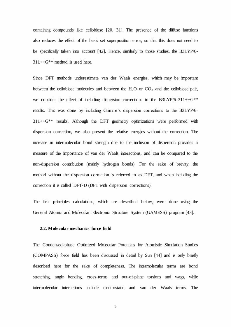
5

containing compounds like cellobiose [20, 31]. The presence of the diffuse functions

also reduces the effect of the basis set superposition error, so that this does not need to

be specifically taken into account [42]. Hence, similarly to those studies, the B3LYP/6-

311++G** method is used here.

Since DFT methods underestimate van der Waals energies, which may be important

between the cellobiose molecules and between the H2O or CO2 and the cellobiose pair,

we consider the effect of including dispersion corrections to the B3LYP/6-311++G**

results. This was done by including Grimme’s dispersion corrections to the B3LYP/6-

311++G** results. Although the DFT geometry optimizations were performed with

dispersion correction, we also present the relative energies without the correction. The

increase in intermolecular bond strength due to the inclusion of dispersion provides a

measure of the importance of van der Waals interactions, and can be compared to the

non-dispersion contribution (mainly hydrogen bonds). For the sake of brevity, the

method without the dispersion correction is referred to as DFT, and when including the

correction it is called DFT-D (DFT with dispersion corrections).

The first principles calculations, which are described below, were done using the

General Atomic and Molecular Electronic Structure System (GAMESS) program [43].

2.2. Molecular mechanics force field

The Condensed-phase Optimized Molecular Potentials for Atomistic Simulation Studies

(COMPASS) force field has been discussed in detail by Sun [44] and is only briefly

described here for the sake of completeness. The intramolecular terms are bond

stretching, angle bending, cross-terms and out-of-plane torsions and wags, while

intermolecular interactions include electrostatic and van der Waals terms. The

6

parameters for the intramolecular terms as well as the atomic charges have been fit to ab

initio data and those for the intermolecular terms are fit to experimental data. The fitting

was done for a variety of materials including metals, metal oxides, some metal ions,

inorganic small molecules, most common organics and polymers [45]. This force field

is also suitable for studies of cellulose and cellobiose [26, 27, 46-51]. Calculations done

with this force field were performed using the Materials Studio Software (Accelrys

Software Inc.).

2.3. Simulation methods

As described below, the initial structures for most of the DFT-D geometry optimizations

were obtained from annealing simulations using the COMPASS force field. Since none

of the structures had the H2O or CO2 molecule between the cellobiose molecules (since

this was not a preferred structure according to the COMPASS force field), six DFT-D

geometry optimisations were initialised with the H2O or CO2 between the cellobiose

molecules. These geometries were therefore constructed by hand. The cellobiose

molecules, as well as the H2O or CO2, were initially in their minimum energy structures

and the cellobiose molecules were parallel to each other. The H2O or CO2 was placed

between the centre of masses of the cellobiose molecules or between neighbouring

glucose units, with the separation between the nearest atoms on the H2O / CO2 and the

nearest atom on cellobiose molecules ranging from 1.6 to 4.7 Å (to avoid starting with a

structure that was too high in energy). All of these geometry optimisations resulted in

the H2O or CO2 moving from being between the molecules to the outside of the

cellobiose pair. That is, in the geometry optimised structures the H2O or CO2 bonded to

the outer surface of the cellobiose pair (similar structures are discussed below with

reference to Fig 3 and 5). The same trends were observed when using the COMPASS

7

force field. Hence, the DFT-D and COMPASS methods predict that the H2O or CO2

prefers to bond to the outer surface of the cellobiose pair, and the COMPASS force field

was used to identify many H2O-cellobiose pair and CO2-cellobiose pair local minimum

energy structures, which were used as input for the DFT-D geometry optimisations.

These structures were obtained using simulated annealing. Since the goal was to obtain

different high and low energy local minimum energy structures, 50–100 cycles with 4-8

million simulation steps per cycle were simulated. The Verlet integration algorithm,

which has the advantage of being formally time-reversible [52], was used with a step

size of 1fs. The mid-cycle temperature for the H2O systems was between 300 and

340 K, and for the CO2 systems it was between 170 and 275 K. These temperatures

were sufficiently high to allow for sampling of large regions of configuration space

while still preventing excessive evaporation of the H2O or CO2 molecule from the

cellobiose pair.

Ten geometries were used as input for the annealing to further increase the

configuration space that was sampled. These geometries had different orientations of the

cellobiose molecules relative to each other (parallel, anti-parallel, perpendicular and

when one of the cellobiose was rotated so that there was a 90° angle between the

molecular planes of the cellobiose molecules) and where the H2O or CO2 molecule was

placed between the cellobiose molecules or at different sites on the surface of the

cellobiose pair. These structures were geometry optimised before being used as input

for the annealing simulations. The choice of the annealing parameters enabled

identification of local minimum energy structures from all of these regions of

configuration space, and many of the annealed structures obtained from the different

8

initial structures were very similar (i.e., the annealing linked the regions of

configuration space spanned by the initial structures).

Ten geometries were typically chosen from each of the ten annealing simulations for

further analysis. The selection was done so that both high and low energy (including the

lowest energy) structures were included. These structures were geometry optimised with

the COMPASS force field using a combination of conjugate gradient [53], Newton [54]

and steepest descent [55] methods. The structures were considered to be minimized

once the change in energy between subsequent steps was less than 2.0×10-5 kcal/mol.

Since some of these structures were the same, this procedure resulted in 90 unique

structures for the H2O-cellobiose pair and 80 unique structures for the CO2-cellobiose

pair. These structures were used as input for the DFT-D geometry optimisations. These

geometry optimizations were performed using a gradient convergence tolerance of

6.28×10-3 kcal/(mol×bohr) and a RMS gradient tolerance of 2.09×10-3 kcal/(mol×bohr).

2.4. Analysis

Several parameters were analysed to ascertain whether H2O and CO2 induced

significantly different local minimum energy structures. These included the relative

energies of the cellobiose pair and the size of the dispersion correction for the different

structures. Several geometrical parameters were analysed (e.g., the relative orientation

of the cellobiose molecules, the relative positioning of the reducing and non-reducing

ends, the orientation of the carbonyl groups, the positions of the H2O and CO2

molecules), but the clearest difference between the high and low energy geometries was

the number of hydrogen-bonds (H-bonds) that linked the two cellobiose molecules.

Hence, this is discussed in detail below, where the H-bond is defined by a maximum

separation of 2.5 Å between the H and O atoms on the different molecules and a

9

minimum angle of 90° formed by the H--O bond on one molecule and the H atom on

the second molecule. The trends discussed below are not expected to be sensitive to this

definition.

The strength of the H2O / CO2 – cellobiose pair interaction is

E(X-pair) = E(X+pair)- Epair- EX Eq. (1)

where E(X+pair) is the energy of the geometry optimised structure, Epair is the energy of

the cellobiose pair and EX is the energy of the H2O or CO2. The cellobiose pair structure

(used to obtain Epair) was subsequently used to obtain the intermolecular energy between

the cellobiose molecules, which is

E(inter-cellob) = Epair- ECellob.1- ECellob.2 Eq. (2)

where ECellob.1 and ECellob.2 are the energies of the separated cellobiose molecules. Note

that the structures used to obtain Epair, ECellob.1 and ECellob.2 were the same as those

obtained from geometry optimisation of H2O / CO2 – cellobiose pair system (i.e., there

was no further optimisation of the individual cellobiose molecules or the cellobiose

pair). This was done since the aim was to analyse the strength of the intermolecular

interactions in the H2O / CO2 – cellobiose pair complex, and further geometry

optimisation would also have included the contribution of the intramolecular energies.

As discussed below, comparison between the DFT and DFT-D results reveals the

relative importance of the non-dispersion and dispersion interactions.

The conformation (anti or syn) of the cellobiose was also analysed since it is known that

it is syn in the cellulose crystal structure and anti in the cellobiose structure in vacuum.

Possible changes from syn to anti will be important during steam or SC-CO2 explosion

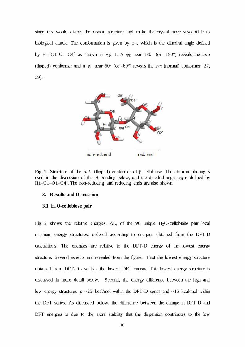
10

since this would distort the crystal structure and make the crystal more susceptible to

biological attack. The conformation is given by φH, which is the dihedral angle defined

by H1–C1–O1–C4´ as shown in Fig 1. A φH near 180° (or -180°) reveals the anti

(flipped) conformer and a φH near 60° (or -60°) reveals the syn (normal) conformer [27,

39].

Fig 1. Structure of the anti (flipped) conformer of β-cellobiose. The atom numbering is

used in the discussion of the H-bonding below, and the dihedral angle φH is defined by H1–C1–O1–C4´. The non-reducing and reducing ends are also shown.

3. Results and Discussion

3.1. H2O-cellobiose pair

Fig 2 shows the relative energies, ΔE, of the 90 unique H2O-cellobiose pair local

minimum energy structures, ordered according to energies obtained from the DFT-D

calculations. The energies are relative to the DFT-D energy of the lowest energy

structure. Several aspects are revealed from the figure. First the lowest energy structure

obtained from DFT-D also has the lowest DFT energy. This lowest energy structure is

discussed in more detail below. Second, the energy difference between the high and

low energy structures is ~25 kcal/mol within the DFT-D series and ~15 kcal/mol within

the DFT series. As discussed below, the difference between the change in DFT-D and

DFT energies is due to the extra stability that the dispersion contributes to the low

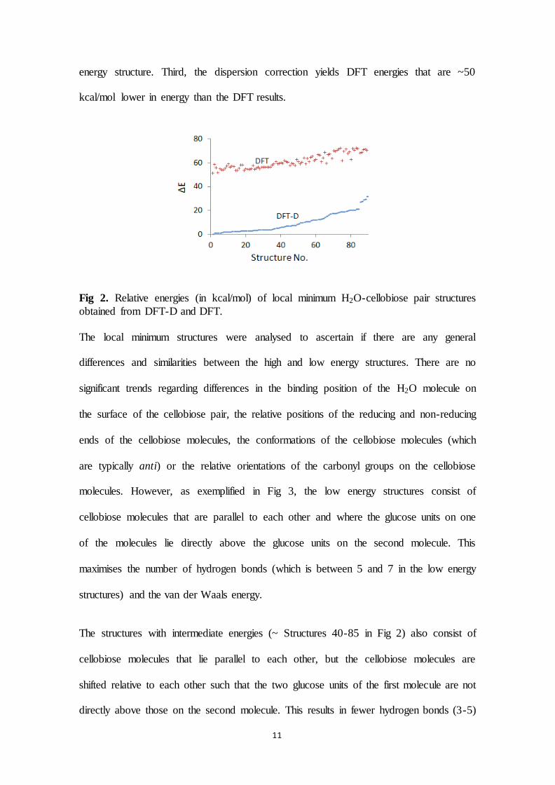
11

energy structure. Third, the dispersion correction yields DFT energies that are ~50

kcal/mol lower in energy than the DFT results.

Fig 2. Relative energies (in kcal/mol) of local minimum H2O-cellobiose pair structures

obtained from DFT-D and DFT.

The local minimum structures were analysed to ascertain if there are any general

differences and similarities between the high and low energy structures. There are no

significant trends regarding differences in the binding position of the H2O molecule on

the surface of the cellobiose pair, the relative positions of the reducing and non-reducing

ends of the cellobiose molecules, the conformations of the cellobiose molecules (which

are typically anti) or the relative orientations of the carbonyl groups on the cellobiose

molecules. However, as exemplified in Fig 3, the low energy structures consist of

cellobiose molecules that are parallel to each other and where the glucose units on one

of the molecules lie directly above the glucose units on the second molecule. This

maximises the number of hydrogen bonds (which is between 5 and 7 in the low energy

structures) and the van der Waals energy.

The structures with intermediate energies (~ Structures 40-85 in Fig 2) also consist of

cellobiose molecules that lie parallel to each other, but the cellobiose molecules are

shifted relative to each other such that the two glucose units of the first molecule are not

directly above those on the second molecule. This results in fewer hydrogen bonds (3-5)

12

and reduced van der Waals attraction. The cellobiose molecules in the structures with

the highest energies have almost no overlap of the glucose units. There are only 1 or 2

hydrogen bonds and the van der Waals interactions are far weaker (as quantified below).

Table 1 lists bond lengths, angles and torsions of the two cellobiose molecules in the

minimum energy structure shown in Fig 3. The data in the table were chosen since they

represent different types of bonds, angles and torsions. It is evident that the bond

lengths and angles are similar for the two cellobiose molecules. The torsion angles that

are formed by carbon and oxygen atoms are also similar, whereas torsion angles that

end with a hydrogen atom can show a significant difference between the two molecules

(e.g., C5´-C6´-O6´-H). This is expected since the hydrogen atoms readily rotate

between local minimum structures that have similar energies so that the intermolecular

interactions- including H-bonding- are strengthened. The separation between the

cellobiose centres of mass is 4.59 Å. Both cellobiose molecules have the anti

conformation, with φH = -173.7 and 179.2° for Cellob.1 and Cellob.2, respectively.

13

Table 1. Representative bond lengths (Å), bond angles (°) and torsions (°) in the cellobiose molecules (Cellob.1 and Cellob.2 in Fig 3) of the DFT-D minimum energy structure.

Cellob.1 Cellob.2

Bond lengths

O1-C4´ 1.436 1.435

C4´-C5´ 1.543 1.546

C5´- O5´ 1.432 1.436

O6´-C6´ 1.423 1.417

O1´-C1´ 1.389 1.401

Angles

C1-O1-C4´ 120 118

O1-C4´-C5´ 110 108

C4´-C5´-O5´ 110 112

C4´-C5´-C6´ 114 114

O5´-C1´-O1´ 109 108

Torsions

C1-O1-C4´-C5´ 118 123

O1-C4´-C5´-O5´ 173 169

C4´-C5´-O5´-C1´ 63 54

C4´-C5´-C6´-O6´ 57 56

C5´-O5´-C1´-O1´ 176 179

O5´-C1´-C2´-O2´ 174 176

C5´-C6´-O6´-H 102 60

O5´-C1´-O1´-H 75 64

C1´-C2´-O2´-H 61 93

Fig 3. Lowest energy H2O-cellobiose pair structure obtained from DFT-D. The H2O molecule is shown in blue. The reducing and non-reducing ends of each cellobiose molecule are shown.

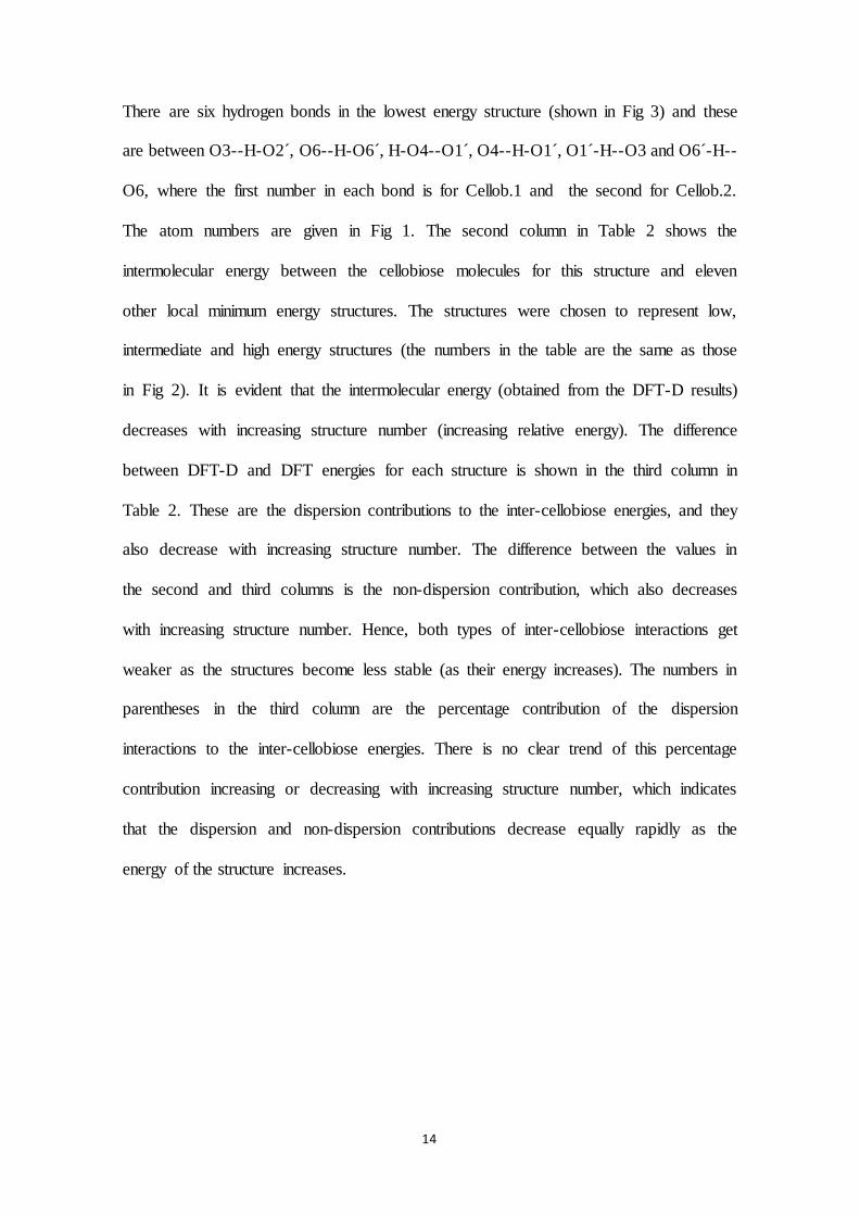
14

There are six hydrogen bonds in the lowest energy structure (shown in Fig 3) and these

are between O3--H-O2´, O6--H-O6´, H-O4--O1´, O4--H-O1´, O1´-H--O3 and O6´-H--

O6, where the first number in each bond is for Cellob.1 and the second for Cellob.2.

The atom numbers are given in Fig 1. The second column in Table 2 shows the

intermolecular energy between the cellobiose molecules for this structure and eleven

other local minimum energy structures. The structures were chosen to represent low,

intermediate and high energy structures (the numbers in the table are the same as those

in Fig 2). It is evident that the intermolecular energy (obtained from the DFT-D results)

decreases with increasing structure number (increasing relative energy). The difference

between DFT-D and DFT energies for each structure is shown in the third column in

Table 2. These are the dispersion contributions to the inter-cellobiose energies, and they

also decrease with increasing structure number. The difference between the values in

the second and third columns is the non-dispersion contribution, which also decreases

with increasing structure number. Hence, both types of inter-cellobiose interactions get

weaker as the structures become less stable (as their energy increases). The numbers in

parentheses in the third column are the percentage contribution of the dispersion

interactions to the inter-cellobiose energies. There is no clear trend of this percentage

contribution increasing or decreasing with increasing structure number, which indicates

that the dispersion and non-dispersion contributions decrease equally rapidly as the

energy of the structure increases.

15

Table 2. Cellobiose- cellobiose intermolecular energies (Einter-pair) and the dispersion correction energies (Edisp) in kcal/mol for some structures shown in Fig 2.

Structure No. Einter-pair Edisp (%)

1 -51.5 -17.8 (35)

6 -46.8 -18.5 (40) 14 -51.2 -17.6 (34) 37 -42.2 -20.8 (49)

40 -27.4 -11.2 (41) 46 -38.2 -14.6 (38)

48 -33.0 -20.3 (62) 78 -34.6 -16.7 (48) 82 -29.4 -18.6 (63)

86 -12.6 -9.7 (77) 88 -13.8 -4.4 (32)

90 -17.3 -6.3 (36)

The H2O molecule is attached to the cellobiose pair by two hydrogen bonds in the

minimum energy structure shown in Figure 1. The H-bonds are with the H-O3 and the

O2 atoms of Cellob.2 shown in Figure 3, and the distance between centre of masses of

H2O and Cellob.2 is 5.63 Å. The intermolecular energy between the H2O and the

cellulose pair is -15.5 kcal/mol. As mentioned above, there are no clear trends of

changes in this energy as the total energy of the H2O-cellobiose pair structure increases.

For example, the energy between the H2O and the cellulose pair is -14.1 kcal/mol for

Structure 46, and it is -18.2 kcal/mol for Structure 88.

3.2. CO2-cellobiose pair

The trends observed for the H2O-cellobiose pair systems are also seen for the CO2-

cellobiose pair systems. Fig 4 shows the relative energies of the 80 unique CO2-

cellobiose pair local minimum energy structures. The minimum energy structure

obtained from the DFT-D calculations is also the DFT minimum energy structure, and

the trend of increasing relative energies from Structures 1 through 80 is the same for

DFT-D and DFT calculations. The difference in DFT-D energies between the highest

and lowest energies structures is ~25 kcal/mol (which was the same for the H2O-

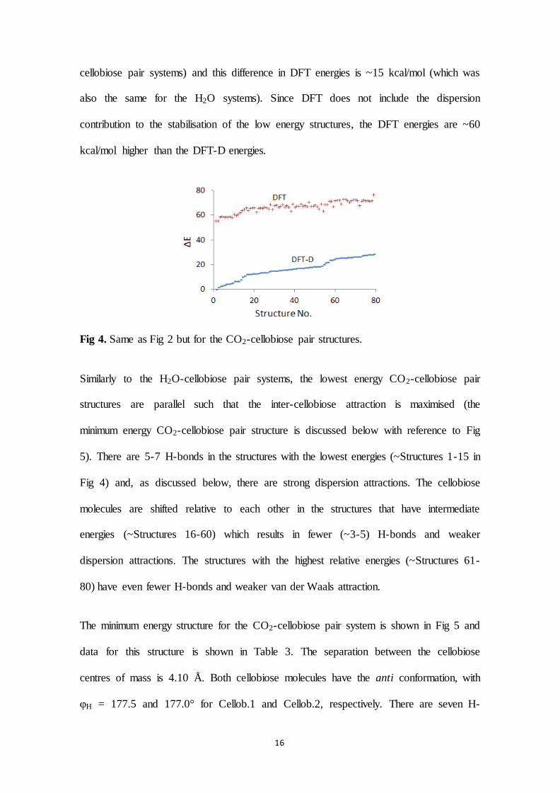
16

cellobiose pair systems) and this difference in DFT energies is ~15 kcal/mol (which was

also the same for the H2O systems). Since DFT does not include the dispersion

contribution to the stabilisation of the low energy structures, the DFT energies are ~60

kcal/mol higher than the DFT-D energies.

Fig 4. Same as Fig 2 but for the CO2-cellobiose pair structures.

Similarly to the H2O-cellobiose pair systems, the lowest energy CO2-cellobiose pair

structures are parallel such that the inter-cellobiose attraction is maximised (the

minimum energy CO2-cellobiose pair structure is discussed below with reference to Fig

5). There are 5-7 H-bonds in the structures with the lowest energies (~Structures 1-15 in

Fig 4) and, as discussed below, there are strong dispersion attractions. The cellobiose

molecules are shifted relative to each other in the structures that have intermediate

energies (~Structures 16-60) which results in fewer (~3-5) H-bonds and weaker

dispersion attractions. The structures with the highest relative energies (~Structures 61-

80) have even fewer H-bonds and weaker van der Waals attraction.

The minimum energy structure for the CO2-cellobiose pair system is shown in Fig 5 and

data for this structure is shown in Table 3. The separation between the cellobiose

centres of mass is 4.10 Å. Both cellobiose molecules have the anti conformation, with

φH = 177.5 and 177.0° for Cellob.1 and Cellob.2, respectively. There are seven H-

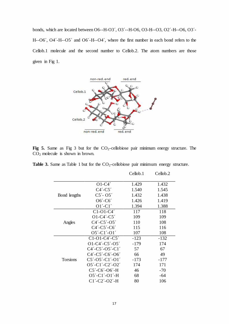
17

bonds, which are located between O6--H-O3´, O3´--H-O6, O3-H--O3, O2´-H--O6, O3´-

H--O6´, O4´-H--O5´ and O6´-H--O4´, where the first number in each bond refers to the

Cellob.1 molecule and the second number to Cellob.2. The atom numbers are those

given in Fig 1.

Fig 5. Same as Fig 3 but for the CO2-cellobiose pair minimum energy structure. The

CO2 molecule is shown in brown.

Table 3. Same as Table 1 but for the CO2-cellobiose pair minimum energy structure.

Cellob.1 Cellob.2

Bond lengths

O1-C4´ 1.429 1.432

C4´-C5´ 1.540 1.545

C5´- O5´ 1.432 1.438

O6´-C6´ 1.426 1.419

O1´-C1´ 1.394 1.388

Angles

C1-O1-C4´ 117 118 O1-C4´-C5´ 109 109

C4´-C5´-O5´ 110 108 C4´-C5´-C6´ 115 116 O5´-C1´-O1´ 107 108

Torsions

C1-O1-C4´-C5´ -123 -132

O1-C4´-C5´-O5´ -179 174 C4´-C5´-O5´-C1´ 57 67

C4´-C5´-C6´-O6´ 66 49 C5´-O5´-C1´-O1´ -173 -177 O5´-C1´-C2´-O2´ 174 171

C5´-C6´-O6´-H 46 -70 O5´-C1´-O1´-H 68 -64

C1´-C2´-O2´-H 80 106

18

It is evident from Table 3 that the structures of Cellob.1 and Cellob.2 (Fig 5) are very

similar. The only large differences are in some of the torsion angles that have hydrogen

as an end atom. As discussed above with reference to the H2O-cellobiose pair system,

this is because there is a small torsion barrier between these local minima, and the

energy difference between the minima is also small.

The second column in Table 4 shows that the inter-cellobiose energy decreases with

increasing structure number (i.e., with increasing relative energy). The dispersion

energy and the non-dispersion contribution to the intermolecular energy (difference

between columns two and three) also decrease. Similarly to the H2O-cellobiose pair

systems, there is no clear evidence that the relative contribution of the dispersion energy

(shown as percent in parenthesis in the table) either increases or decreases with

increasing structure number.

Table 4. Same as Table 2 but for CO2-cellobiose pair systems.

Structure No. Einter-pair Edisp (%)

1 -56.6 -23.3 (41)

3 -54.9 -22.4 (41)

11 -46.7 -19.1 (41)

19 -38.0 -20.7 (54)

21 -34.0 -13.4 (39)

22 -25.6 -17.8 (70)

28 -30.2 -20.0 (66)

34 -29.4 -19.2 (65)

46 -23.6 -12.2 (52)

54 -18.9 -6.0 (32)

65 -12.9 -11.2 (87)

72 -17.4 -6.1 (35)

The distance between the centre of mass of the CO2 molecule and the cellobiose pair in

the minimum energy structure shown in Fig 5 is 7.51 Å. Neither this distance, nor the

CO2-cellobiose intermolecular energy, shows a systematic change with increasing

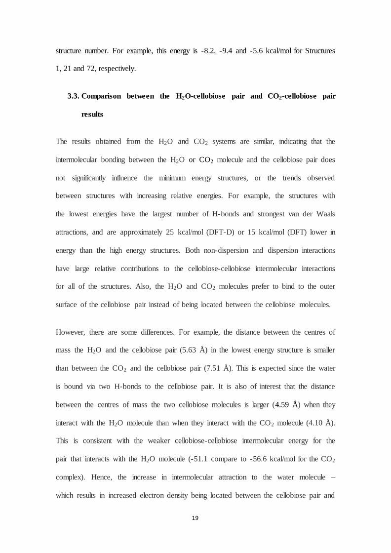
19

structure number. For example, this energy is -8.2, -9.4 and -5.6 kcal/mol for Structures

1, 21 and 72, respectively.

3.3. Comparison between the H2O-cellobiose pair and CO2-cellobiose pair

results

The results obtained from the H2O and CO2 systems are similar, indicating that the

intermolecular bonding between the H2O or CO2 molecule and the cellobiose pair does

not significantly influence the minimum energy structures, or the trends observed

between structures with increasing relative energies. For example, the structures with

the lowest energies have the largest number of H-bonds and strongest van der Waals

attractions, and are approximately 25 kcal/mol (DFT-D) or 15 kcal/mol (DFT) lower in

energy than the high energy structures. Both non-dispersion and dispersion interactions

have large relative contributions to the cellobiose-cellobiose intermolecular interactions

for all of the structures. Also, the H2O and CO2 molecules prefer to bind to the outer

surface of the cellobiose pair instead of being located between the cellobiose molecules.

However, there are some differences. For example, the distance between the centres of

mass the H2O and the cellobiose pair (5.63 Å) in the lowest energy structure is smaller

than between the CO2 and the cellobiose pair (7.51 Å). This is expected since the water

is bound via two H-bonds to the cellobiose pair. It is also of interest that the distance

between the centres of mass the two cellobiose molecules is larger (4.59 Å) when they

interact with the H2O molecule than when they interact with the CO2 molecule (4.10 Å).

This is consistent with the weaker cellobiose-cellobiose intermolecular energy for the

pair that interacts with the H2O molecule (-51.1 compare to -56.6 kcal/mol for the CO2

complex). Hence, the increase in intermolecular attraction to the water molecule –

which results in increased electron density being located between the cellobiose pair and

20

the water molecule – decreases the interaction strength (electron density) between the

cellobiose molecules.

4. Conclusion

Previous studies [26, 27] have shown that the B3LYP/6-311++G** density functional

method yields valid energies and structures for cellobiose and H2O-cellobiose systems.

This method, including Grimme’s dispersion correction, was used to study the

interactions between H2O and two cellobiose molecules, as well as CO2 and two

cellobiose molecules. The results obtained with and without the dispersion corrections

are presented, since they enable an estimation of the relative contributions of non-

dispersion (main H-bonding) and dispersion (van der Waals bonding) terms to the

intermolecular energies.

Geometry optimisation with the DFT-D method showed that the H2O and CO2

molecules prefer to bond to the surface of the cellobiose pair as opposed to being

located between the cellobiose molecules. Also, comparison of 90 unique H2O-

cellobiose pair and 80 unique CO2-cellobiose pair local minimum energy structures

showed that the trends in relative energies between the low and high energy structures

were the same with and without dispersion correction. The structures with lower

energies typically have a larger number of H-bonds and stronger van der Waals

interactions.

Comparison of the DFT and DFT-D cellobiose-cellobiose intermolecular energies

showed that both the non-dispersion and dispersion terms have large contributions to

the intermolecular energies. The contribution of the dispersion (and non-dispersion)

21

energies was typically between 30 and 70 %, and there was no clear trend in increasing

or decreasing this contribution with weaker intermolecular bonds.

The distance between the centres of mass the two cellobiose molecules is larger (4.59

Å) when they interact with the H2O molecule than when they interact with the CO2

molecule (4.10 Å). This is consistent with the weaker cellobiose-cellobiose

intermolecular energy for the pair that interacts with the H2O molecule. Hence, the

increase in intermolecular attraction to the water molecule – which results in increased

electron density being located between the cellobiose pair and the water molecule –

decreases the interaction strength between the cellobiose molecules.

5. Acknowledgments

Financial support from Stiftelsen Föreningssparbanken Sjuhärad and The Carl Trygger

Foundation for Scientific Research is gratefully acknowledged. GAMESS-US, version 1

OCT 2010 (R1) was used at the high performance computer cluster Kalkyl at UPPMAX

(Uppsala Multidisciplinary Centre for Advanced Computational Science), Uppsala

Sweden. Calculations using the COMPASS force field were done using the program

from Accelrys Software Inc.

22

References

[1] Zhang Q, Bulone V, Ågren H, Tu Y (2011) A molecular dynamics study of the

thermal response of crystalline cellulose Iβ. Cellulose 18: 207–221

[2] Wyman C E (2007) What is (and is not) vital to advancing cellulosic ethanol. Trends

Biotechnol 25: 153–157

[3] Taherzadeh M J, Karimi K (2008) Pretreatment of lignocellulosic wastes to improve ethanol and biogas production: a review. Int. J. Mol. Sci. 9: 1621-1651

[4] Fan L T, Lee Y, Beardmore D H (1980) Mechanism of the enzymatic hydrolysis of cellulose: effects of major structural features of cellulose on enzymatic hydrolysis.

Biotechnol. Bioeng. 22: 177-199

[5] Wyman C E (1996) 1: Ethanol production from lignocellulosic biomass: overview. In: Wyman C E (ed) Handbook on bioethanol: production and utilization, Taylor &

Francis, Washington DC, USA, pp 1-18

[6] Mason W H (1926) Process and apparatus for disintegration of wood and the like. US Pat. 1578609

[7] Babcock L W (1932) Method of producing fermentable sugars and alcohol from

wood. US Pat. 1855464

[8] Dahman Y, Volynets B (2011) Assessment of pretreatments and enzymatic hydrolysis of wheat straw as a sugar source for bioprocess industry. International Journal of Energy and Environment (IJEE) 2: 427–446

[9] Martin-Sampedro R , Rojas O J, Capanema E A, Hoeger I, Villar J C (2011) Lignin changes after steam explosion and laccase-mediator treatment of eucalyptus wood chips. J. Agric. Food Chem. 59: 8761–8769

[10] Jedvert K, Theliander H, Saltberg A, Lindström M E (2012) Mild steam explosion

and chemical pre-treatment of Norway spruce. BioResources 7: 2051–2074

[11] Chacha N, Toven K, Mtui, G, Katima J, Mrema G (2011) Steam pretreatment of pine (Pinus patula) wood residue for the production of reducing sugars. Cellulose

Chemistry and Technology 45: 495–501

[12] Kumar P, Barrett D M, Delwiche M J, Stroeve P (2009) Methods for pretreatment of lignocellulosic biomass for efficient hydrolysis and biofuel production. Ind. Eng.

Chem. Res. 48: 3713–3729

[13] Zheng Y, Lin H M, Wen J, Cao N, Yu X, Tsao GT (1995) Supercritical carbon dioxide explosion as a pretreatment for cellulose hydrolysis. Biotechnol Lett 17:845-850

23

[14] Zheng Y, Tsao GT (1996) Avisel hydrolysis by cellulose enzyme in supercritical CO2. Biotechnol. Lett. 18: 451-454

[15] Zheng Y, Lin H, Tsao G T (1998) Pretreatment for cellulose hydrolysis by carbon dioxide explosion. Biotechnol Prog. 14: 890–896

[16] Narayanaswamya N, Faik A, Goetz D J, Gu T (2011) Supercritical carbon dioxide

pretreatment of corn stover and switchgrass for lignocellulosic ethanol production. Bioresour. Technol. 102 : 6995–7000

[17] Alinia R, Zabihi S, Esmaeilzadeh F, Fathi Kalajahi (2010) Pretreatment of wheat

straw by supercritical CO2 and its enzymatic hydrolysis for sugar production. J. Biosystems Eng. 107: 61–66

[18] Muratov G, Kim C (2002) Enzymatic hydrolysis of cotton fibers in supercritical

CO2. Biotechnol. Bioprocess Eng. 7: 85–88

[19] Gua T, Held M A, Faikc A (2013) Supercritical CO2 and ionic liquids for the pretreatment of lignocellulosic biomass in bioethanol production Environ. Technol.34, 1735–1749

[20] Stortz C A, Johnson G P, French A D, Csonka G I (2009) Comparison of different force fields for the study of disaccharides. J. Carbohydr. Res. 344: 2217–2228

[21] Bergenstråhle M, Matthews J, Crowley M, Brady J (2010) Cellulose crystal structure and force fields. International Conference on Nanotechnology for the forest

products industry. Otaniemi, Espoo, Finland

[22] Payal R S, Bharath R, Periyasamy G, Balasubramanian S (2012) Density functional theory investigations on the structure and dissolution mechanisms for cellobiose and

xylan in an ionic liquid: Gas phase and cluster calculations. J. Phys. Chem. B 116: 833–840

[23] Momany F A, Schnupf U (2011) DFTMD studies of β-cellobiose: conformational preference using implicit solvent. Carbohydr. Res. 346: 619–630

[24] French A D, Johnson G P (2006) Quantum mechanics studies of cellobiose conformations. Can J Chem. 84: 603–612

[25] French A D, Johnson G P (2008) Roles of starting geometries in quantum mechanics studies of cellobiose. Mol. Simul. 34: 365–372

[26] Bazooyar F, Taherzadeh M, Niklasson C, Bolton K (2013) Molecular Modelling of

Cellulose Dissolution. J. Comput. Theor. Nanosc. 10: 2639-2646

[27] Bazooyar F, Momany F A, Bolton K (2012) Validating empirical force fields for molecular-level simulation of cellulose dissolution. Comput. Theor. Chem. 984: 119–

127

24

[28] Strati G L, Willett J L, Momany F A (2002) Ab initio computational study of β-cellobiose conformers using B3LYP/6-311++ G**. Carbohydr. Res. 337: 1833-1849

[29] Strati G L, Willett J L, Momany F A (2002) A DFT/ab initio study of hydrogen bonding and conformational preference in model cellobiose analogs using B3LYP/6-

311++ G**. Carbohydr. Res. 337: 1851-1859

[30] Bosma W B, Appell M, Willett J L, Momany F A (2006) Stepwise hydration of cellobiose by DFT methods: 2. Energy contributions to relative stabilities of cellobiose

(H2 O) 1–4 complexes. THEOCHEM. 776: 1–19

[31] Momany F A, Willett J L (2000) Computational studies on carbohydrates: I. Density functional ab initio geometry optimization on maltose conformations. J.

Comput. Chem. 21: 1204–1219

[32] French A D, Johnson G P (2004) Advanced conformational energy surfaces for cellobiose**. Cellulose 11: 449–462

[33] Aldred P http://www.accelrys.com/resource-center/case-studies /archive /studies /cellulose.html. Accessed 12 April 2014

[34] Bazooyar F, Bolton K (2014) Molecular-level simulations of cellulose steam explosion. Quantum Matter, in press

[35] Grimme S (2004) Accurate description of van der Waals complexes by density functional theory including empirical corrections. J. Comput. Chem. 25: 1463–1473

[36] Piacenza M, Grimme S (2005) Van der Waals interactions in aromatic systems:

structure and energetics of dimers and trimers of pyridine. ChemPhysChem. 6: 1554– 1558

[37] Grimme S (2006) Semiempirical GGA‐type density functional constructed with a

long‐range dispersion correction. J. Comput. Chem. 27: 1787–1799

[38] Becke A D (1993) Density‐functional thermochemistry. III. The role of exact

exchange. J. Chem. Phys. 98: 5648

[39] Lee C, Yang W, Parr R G (1998) Development of the Colle-Salvetti correlation-

energy formula into a functional of the electron density. Phys. Rev. B 37: 785–789

[40] Miehlich B, Savin A, Stoll H, Preuss H (1989) Results obtained with the correlation energy density functionals of becke and Lee, Yang and Parr. Chem. Phys.

Lett. 157: 200–206

[41] Stephens P J, Devlin F J, Chabalowski C F, Frisch M J (1994) Ab initio calculation of vibrational absorption and circular dichroism spectra using density functional force fields. J. Phys. Chem. 98: 11623–11627

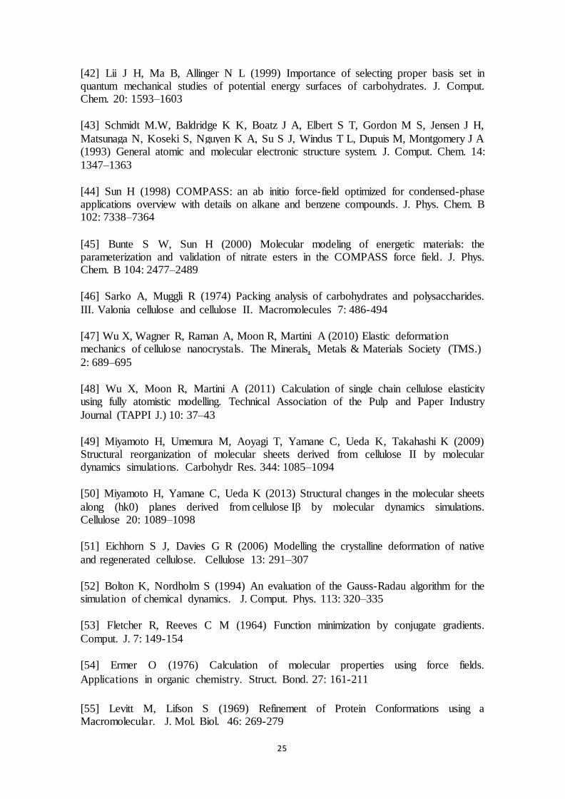
25

[42] Lii J H, Ma B, Allinger N L (1999) Importance of selecting proper basis set in quantum mechanical studies of potential energy surfaces of carbohydrates. J. Comput. Chem. 20: 1593–1603

[43] Schmidt M.W, Baldridge K K, Boatz J A, Elbert S T, Gordon M S, Jensen J H,

Matsunaga N, Koseki S, Nguyen K A, Su S J, Windus T L, Dupuis M, Montgomery J A (1993) General atomic and molecular electronic structure system. J. Comput. Chem. 14:

1347–1363

[44] Sun H (1998) COMPASS: an ab initio force-field optimized for condensed-phase applications overview with details on alkane and benzene compounds. J. Phys. Chem. B 102: 7338–7364

[45] Bunte S W, Sun H (2000) Molecular modeling of energetic materials: the parameterization and validation of nitrate esters in the COMPASS force field. J. Phys. Chem. B 104: 2477–2489

[46] Sarko A, Muggli R (1974) Packing analysis of carbohydrates and polysaccharides.

III. Valonia cellulose and cellulose II. Macromolecules 7: 486-494

[47] Wu X, Wagner R, Raman A, Moon R, Martini A (2010) Elastic deformation mechanics of cellulose nanocrystals. The Minerals, Metals & Materials Society (TMS.)

2: 689–695

[48] Wu X, Moon R, Martini A (2011) Calculation of single chain cellulose elasticity using fully atomistic modelling. Technical Association of the Pulp and Paper Industry

Journal (TAPPI J.) 10: 37–43

[49] Miyamoto H, Umemura M, Aoyagi T, Yamane C, Ueda K, Takahashi K (2009) Structural reorganization of molecular sheets derived from cellulose II by molecular dynamics simulations. Carbohydr Res. 344: 1085–1094

[50] Miyamoto H, Yamane C, Ueda K (2013) Structural changes in the molecular sheets

along (hk0) planes derived from cellulose Iβ by molecular dynamics simulations. Cellulose 20: 1089–1098

[51] Eichhorn S J, Davies G R (2006) Modelling the crystalline deformation of native

and regenerated cellulose. Cellulose 13: 291–307

[52] Bolton K, Nordholm S (1994) An evaluation of the Gauss-Radau algorithm for the simulation of chemical dynamics. J. Comput. Phys. 113: 320–335

[53] Fletcher R, Reeves C M (1964) Function minimization by conjugate gradients.

Comput. J. 7: 149-154

[54] Ermer O (1976) Calculation of molecular properties using force fields.

Applications in organic chemistry. Struct. Bond. 27: 161-211

[55] Levitt M, Lifson S (1969) Refinement of Protein Conformations using a Macromolecular. J. Mol. Biol. 46: 269-279

26

Paper V

1

Molecular-level Calculations of Cellulose Explosion using Supercritical CO2

Faranak Bazooyar1, 2,∗, Martin Bohlén1, Mohammad Taherzadeh1, Claes Niklasson2

and Kim Bolton1

1Swedish Centre for Resource Recovery, University of Borås, SE-501 90, Borås, Sweden 2Department of Chemical Engineering, Chalmers University of Technology, Gothenburg,

SE-412 96, Sweden

Abstract

Supercritical carbon dioxide (SC-CO2) explosion is often used as a pretreatment step when

converting cellulosic waste into biofuel. Density functional theory with dispersion correction

(DFT-D), grand canonical Monte Carlo (GCMC) and molecular dynamics (MD) have been

used to study the explosion of crystalline cellulose at temperature/pressure combinations

relevant to experimental studies. The GCMC and MD simulations are based on the

COMPASS force field, which provides a valid description of the cellulose crystal structure.

In addition, comparison of COMPASS and DFT-D minimum energy structures and energies

of CO2 interacting with a cellobiose pair, shows that the COMPASS force field correctly

predicts that compact structures – where there is strong intermolecular bonding between the

cellobiose molecules – have lower energies than structures that resemble the amorphous

phase. The simulations show significant disruption of the crystal structure during the loading

of SC-CO2, and subsequent explosion does not lead to additional significant distortion of the

crystal structure. This is observed, for example, by large changes in the centres of mass of

cellulose chains from the centre of the crystal structure, as well as increased separation of the

non-reducing and reducing ends of chains from the neighbouring chains. Increasing the

∗ Corresponding author. Tel: +46 33 435 45 34. E-mail address: faranak.bazooyar@hb.se

2

pressure decreases disruption of the crystal structure, while increasing temperature typically

increases the displacement of cellulose chains. There is no significant correlation between the

change in centres of mass of the chains and changes in their radii of gyration. The extent of

disruption observed in the simulations is less than that observed for steam explosion (under

conditions that are relevant to experimental studies of steam explosion).

Keywords: cellulose, density functional theory with dispersion correction, molecular

dynamics, grand canonical Monte Carlo, super critical CO2 explosion

1. Introduction

Continued depletion of fossil fuels, increasing energy demands and the negative

environmental impacts of current fuel usage requires the identification and development of

new energy sources. Lignocellulosic materials are the most abundant resources that can be

converted into biofuels, but the crystalline structure of cellulose as well as the presence of

lignin and hemicellulose hinders enzymatic hydrolysis [1].

The most important lignocellulosic biomass constituents are lignin, hemicellulose and

cellulose. The relative quantities of these components vary depending on the feedstock, but

are typically 15-25 % lignin, 23- 32 % hemicellulose and 38- 50 % cellulose, in addition to

the extractives and inorganic materials [2]. Accessibility of the hemicellulose and cellulose is

crucial for enzymolysis, where the cellulose chains are cut into β-(1, 4)-D-glucan units for

subsequent fermentation. Different chemical, physical and physico-chemical pretreatment

methods have been used to remove lignin and hemicellulose, as well as to disrupt the

crystalline cellulose material that is required to increase the accessibility of the cellulose

chains to enzyme attack.

3

Ding and Himmel [3] have suggested a cellulose structure where each elementary fibril

contains thirty-six cellulose chains. In this model, which is shown in Fig. 1, the outermost

layer contains eighteen chains (green) that surround eighteen inner cellulose chains. The

inner chains contain of six core chains (shown as brown) that are bonded to twelve chains in

the middle shell (orange). As reported previously [4], both hydrogen and van der Waals

interactions are important for the intermolecular bonding between the chains.

Figure 1- Cross section of a cellulose elementary fibril containing thirty-six cellulose chains

[3].

Supercritical fluids are widely used for separating and purifying high value products [5], and

pretreatment of cellulose-containing materials using supercritical fluids enhances enzymatic

hydrolysis [6]. For example, in 1995 Zheng [7] proposed that supercritical carbon dioxide

(SC-CO2) could be used as a green solvent for dissolving lignocellulosic biomass. This assists

in biofuel production either with or without explosion. CO2 has a low critical temperature and

pressure (31.1 °C and 1067 psi), and under supercritical conditions the CO2 has gas-like mass

transfer and liquid-like solvating power with low viscosity [8, 9]. In addition, SC-CO2 is

economical, non-flammable, non-toxic and easy to recycle [10]. SC-CO2 explosion enhances

the penetration of chemicals into lignocellulosic materials during pulp production [11]; also

in many pretreatment processes SC-CO2 has been used for materials such as corn stover,

switchgrass, aspen, rice straw, southern yellow pine (SYP), cellulose-containing waste from

4

cotton production, cotton fibre, Avicel, wheat straw, sugarcane bagasse and other feed stocks

[6, 11-20].

Experiments show that the effectiveness of SC-CO2 pretreatment depends on the feedstock.

For example, while pine wood shows no significant change in its microstructure arrangement

during SC-CO2 pretreatment, the method is effective for Avicel and increases the glucose

yield by 50% [17, 21]. It is believed that SC-CO2 pretreatment is effective for Avicel since it

decreases the crystallinity of the cellulose thereby increasing the surface area [17].

Experimental studies have investigated different methods for SC-CO2 pretreatment, both with

and without explosion. They have used different temperature, pressure, and residence time

for different feedstock. For instance, combinations of 40-110 °C/ 1450-4350 psi/ 15-45 min

were used for rice straw [13], 25-80 °C/ 1100-4000 psi/ 60 min were used for bagasse [11],

160-210 °C/ 2900 psi/ 60 min for switch grass [12], 80-160 °C/ 2900 and 3500 psi/ 10-60

min for corn stover [12] and 112-165 °C/ 3100 psi/10-60 min was used for aspen [21] and

SYP [15].

SC-CO2 pretreatment with explosion is comprised of two stages. In the first stage, known as

loading, the feedstock is submersed in CO2 at a supercritical temperature and pressure. In the

second stage, known as explosion, there is a rapid pressure drop to atmospheric pressure. SC-

CO2 explosion not only helps to remove, dissolve and depolymerise the lignin and

hemicellulose, but also reduces the size and crystallinity of the cellulose structure [22].

The effect of varying the temperature and pressure has also been studied for some feedstock.

Increasing the temperature typically improves the conversion of the feedstock to biofuel [19].

Zheng et al. (1998) showed that pretreatment of Avicel with subcritical CO2 at 25 °C gave a

small yield of glucose, and increasing the temperature to 35°C increased the yield

5

significantly. Further increase in temperature did not result in additional enhancement in the

glucose yield [11]. The effect of pressure is not as clear, and appears to depend on the

feedstock. For example, Narayanaswamy et al. showed that increasing SC-CO2 pressure from

2500 to 3500 psi during pretreatment of corn stover doubled the glucose yield [12]. In

contrast, increasing the pressure from 3100 to 4000 psi during pretreatment of aspen resulted

in a lower glucose yield [21].

Many of the SC-CO2 pretreatment methods include water, which is believed to increase the

enzymatic hydrolysis [11]. For example, dry lignocellulosic materials like aspen and SYP

show no significant glucose yield after SC-CO2 pretreatment, but the presence of 40-73%

water increases the yield. More than 73% water content did not show more glucose yield

[21]. The reason for the improved hydrolysis in the presence of water may be due to the

formation of carbonic acid, which may hydrolyse some of the hemicellulose that surrounds

the crystalline cellulose. This would break the cellulose-hemicellulose hydrogen bonds (H-

bonds) and the H-bonds between cellulose microfibrils. A second reason for the improved

hydrolysis in the presence of water is that it may lead to swelling of the biomass, thereby

increasing susceptibility to CO2 penetration [11, 12]. It may also be noted that enzymes are

also active in microaqueous environments [16].

Experimental studies of chemical reaction mechanisms and rates are complemented by

computational studies, which offer easy manipulation and analysis at the molecular level.

These types of calculations are often based on model systems and empirical force fields,

which allows for the study of sufficiently large systems and long times so that statistically

converged results can be obtained under conditions relevant to experiment. It is important

that both the model and the force field provide a valid description of the system [23, 24].

6

This contribution describes the results obtained from density functional theory calculations as

well as Grand Canonical Monte Carlo (GCMC) and molecular dynamics (MD) based on the

COMPASS force field. This force field is first validated for the system studied here by

comparing structures and energies obtained from the force field with those obtained from

density functional theory, and then applied in the GCMC and MD simulations to study the

loading and explosion of a cellulose crystal model using SC-CO2. The crystalline model is

based on a model proposed by Ding and Himmel [25], shown in Fig. 1. The temperature-

pressure combinations that have been studied, (and that) are relevant to experimental studies,

are listed and named A to G in Table 1. Systems A-D enable analysis of the effect of change

in pressure on the CO2 explosion, whereas systems C, E-G enable analysis of the change in

temperature. It can be noted that these studies are based on a model system of a cellulose

crystal, and is the first step in modelling material that contains lignin and hemicellulose. The

studies are therefore more relevant to systems that contain little or no lignin or hemicellulose,

such as Avicel. The simulations also consider SC-CO2 explosion under dry conditions (such

as those used in experimental studies of Avicel) and the effects of including water are left for

future studies.

Table 1- Temperature and pressure of systems A-G.

System Temperature (°C) Pressure (psi) A 110 2500

B 110 3000

C 110 3500

D 110 4000

E 135 3500

F 165 3500

G 200 3500

2. Methods

7

2.1. The COMPASS force field

Molecular-level simulations of cellulose have been based on several force fields, including

PCFF [26], modified charmm02 [27], Hybrid [28], GLYCAM06 [29], GROMOS 45a4 [30]

and Condensed-phase Optimized Molecular Potentials for Atomistic Simulation Studies

(COMPASS) [31]. The COMPASS force field, which was developed to study for a variety of

materials including organic molecules and polymers [32], is used here. As discussed below,

this force field provides a valid description of crystalline cellulose and yields correct

structures and energetic trends for CO2 interacting with a cellobiose pair (cellobiose is the

smallest repeat unit in a cellulose chain). It is described in detail elsewhere [4], and is briefly

presented here for the sake of completeness.

The COMPASS force field includes valence and non-bonded terms. The valence terms

include bond stretching, angle bending, torsions, wags and cross-coupling terms, while non-

bonded interactions are described by LJ 9-6 functions for van der Waals (vdW) interactions

and electrostatic functions for charge-charge interactions. The valence parameters and

electrostatic terms are fitted to ab initio data, while the vdW parameters are derived from

experimental data [32-34].

Several studies have shown that the COMPASS force field yields valid structures and

mechanical properties of cellulose crystal structures [26-30]. For example, Aldred [35]

evaluated the validity of this force field by performing canonical (NVT) MD simulations of

the cellulose Iβ crystal structure. The calculated unit cell parameters, that are shown in Fig. 2,

(a= 7.44 Å, b= 8.02 Å, c= 10.42 Å and γ= 98.33°) deviate by only 5.2, 3.0, 0.4 and 2.1%

from the experimental data (a= 7.85 Å, b= 8.27 Å, c= 10.38 Å and γ= 96.3°) measured by

Sarko and Muggli using X-ray spectroscopy [36].

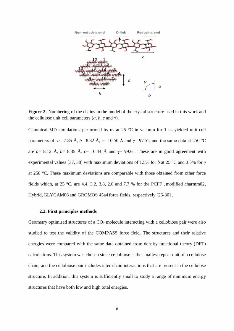
8

Figure 2- Numbering of the chains in the model of the crystal structure used in this work and the cellulose unit cell parameters (a, b, c and γ).

Canonical MD simulations performed by us at 25 °C in vacuum for 1 ns yielded unit cell

parameters of a= 7.85 Å, b= 8.32 Å, c= 10.50 Å and γ= 97.5°, and the same data at 250 °C

are a= 8.12 Å, b= 8.35 Å, c= 10.44 Å and γ= 99.6°. These are in good agreement with

experimental values [37, 38] with maximum deviations of 1.5% for b at 25 °C and 3.3% for γ

at 250 °C. These maximum deviations are comparable with those obtained from other force

fields which, at 25 °C, are 4.4, 3.2, 3.8, 2.0 and 7.7 % for the PCFF , modified charmm02,

Hybrid, GLYCAM06 and GROMOS 45a4 force fields, respectively [26-30] .

2.2. First principles methods

Geometry optimised structures of a CO2 molecule interacting with a cellobiose pair were also

studied to test the validity of the COMPASS force field. The structures and their relative

energies were compared with the same data obtained from density functional theory (DFT)

calculations. This system was chosen since cellobiose is the smallest repeat unit of a cellulose

chain, and the cellobiose pair includes inter-chain interactions that are present in the cellulose

structure. In addition, this system is sufficiently small to study a range of minimum energy

structures that have both low and high total energies.

9

First principles methods are expected to give reasonably accurate data for disaccharides,

including the glycosidic bond strength, which may be affected by the electron pairs on the

oxygen atom that is involved in the bond as well as those of nearby oxygen atoms [39].

Previous studies have shown that, among the different DFT methods, the B3LYP functional

[40-42] combined with a basis set that includes diffuse and polarization terms yields accurate

relative energies and structures of hydroxyl-containing compounds like carbohydrates [23,

43]. The presence of the diffuse functions also reduces the effect of the basis set superposition

error, so that it does not specifically need to be taken into account [44]. Hence, similarly to

these studies, the B3LYP/6-311++G** method is used here.

Since DFT methods underestimate van der Waals energies, which are expected to be

important between the cellobiose molecules and between the CO2 and the cellobiose pair, the

effect of dispersion corrections to the B3LYP/6-311++G**results were studied. This was

done by including Grimme’s dispersion corrections [45-47] in the B3LYP/6-311++G**

calculations. Although the DFT calculations were performed with the dispersion correction,

we also present the relative energies without the correction for comparison. For the sake of

brevity, the relative energies without the dispersion correction are referred to as DFT, and

when including the correction it is called DFT-D (DFT with dispersion corrections). The first

principles calculations were done using the General Atomic and Molecular Electronic

Structure System (GAMESS) program [48].

As described below, the initial structures for most of the DFT-D geometry optimizations were

obtained from annealing simulations using the COMPASS force field. Since none of the

structures had the CO2 molecule between the cellobiose molecules (since this was not a

preferred structure according to the COMPASS force field), three DFT-D geometry

optimisations were initialised with the CO2 between the cellobiose molecules. These

10

geometries were therefore constructed by hand. The CO2 and the cellobiose molecules were

initially in their minimum energy structures and the cellobiose molecules were parallel to

each other (since, as discussed below, this is the energetically preferred cellobiose geometry).

The CO2 was placed between the centre of masses of the cellobiose molecules or between

neighbouring glucose units, with the separation between the nearest atoms on the CO2 and the

nearest atom on cellobiose molecules ranging from 1.6 to 4.7 Å (to avoid starting with a

structure that was too high in energy). All of these geometry optimisations resulted in the

CO2 moving from being between the molecules to the outside of the cellobiose pair. That is,

in the geometry optimised structures the CO2 bonded to the outer surface of the cellobiose

pair (similar structures are discussed below with reference to Fig. 5). The same trends were

observed when using the COMPASS force field. Hence, the DFT-D and COMPASS methods

predict that the CO2 prefers to bond to the outer surface of the cellobiose pair, and the

COMPASS force field was used to identify many CO2-cellobiose pair local minimum energy

structures, which were used as input for the DFT-D geometry optimisations.

These structures were obtained using simulated annealing. Since the goal was to obtain

different high and low energy local minimum energy structures, 50–100 cycles with 4-8

million simulation steps per cycle were simulated. The Verlet integration algorithm, which

has the advantage of being formally time-reversible [49], was used with a step size of 1fs.

The mid-cycle temperature was between 170 and 275 K. These temperatures were

sufficiently high to allow for sampling of large regions of configuration space while still

preventing excessive evaporation of the CO2 molecule from the cellobiose pair.

Ten geometries were used as input for the annealing to further increase the configuration

space that was sampled. These geometries had different orientations of the cellobiose

molecules relative to each other (parallel, anti-parallel, perpendicular and when one of the

11

cellobiose was rotated so that there was a 90° angle between the molecular planes of the

cellobiose molecules) and where the CO2 molecule was placed between the cellobiose

molecules or at different sites on the surface of the cellobiose pair. These structures were

geometry optimised before being used as input for the annealing simulations. The choice of

the annealing parameters enabled identification of local minimum energy structures from all

of these regions of configuration space, and many of the annealed structures obtained from

the different initial structures were very similar (i.e., the annealing linked the regions of

configuration space spanned by the initial structures).

Ten geometries were typically chosen from each of the ten annealing simulations for further

analysis. The selection was done so that both high and low energy (including the lowest

energy) structures were included. These structures were geometry optimised with the

COMPASS force field using a combination of conjugate gradient [50], Newton-Raphson [51]

and steepest descent [52] methods. The structures were considered to be minimized once the

change in energy between subsequent steps was less than 2.0×10-5 kcal/mol. Since some of

these structures were the same, this procedure resulted in 80 unique structures for the CO2-

cellobiose pair. These structures were used as input for the DFT-D geometry optimisations.

These geometry optimizations were performed using a gradient convergence tolerance of

6.28×10-3 kcal/ (mol×Bohr) and a RMS gradient tolerance of 2.09×10-3 kcal/ (mol×Bohr).

2.3. Model of the cellulose crystal

Several models have been proposed for the cellulose crystal structure [23, 24]. As mentioned

above, the model used here is based on the structure of cellulose Iβ proposed by Ding and

Himmel [3] which, as shown in Fig. 1, contains a central core of six cellulose chains

surrounded by a middle and outermost shell. The largest difference between these regions is

that the core and middle shell are surrounded by cellulose chains, whereas the outermost shell

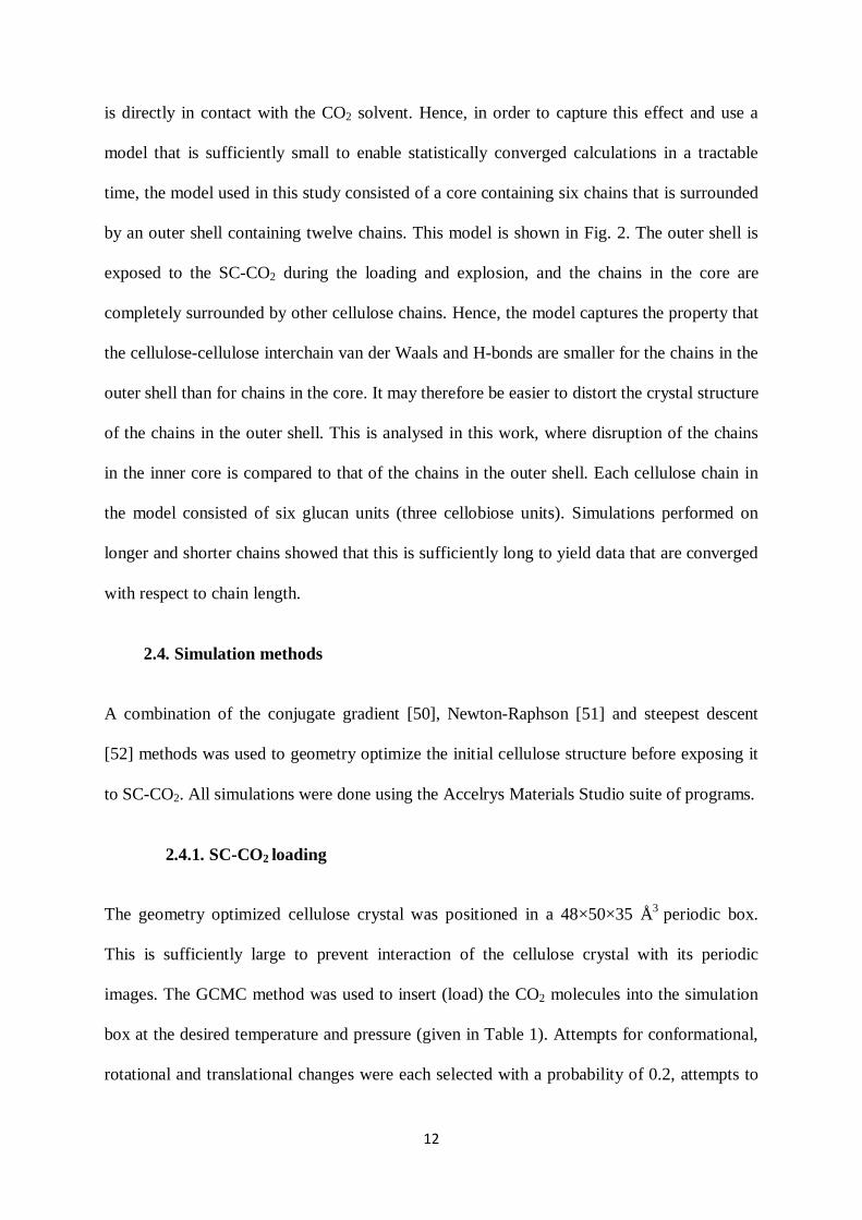
12

is directly in contact with the CO2 solvent. Hence, in order to capture this effect and use a

model that is sufficiently small to enable statistically converged calculations in a tractable

time, the model used in this study consisted of a core containing six chains that is surrounded

by an outer shell containing twelve chains. This model is shown in Fig. 2. The outer shell is

exposed to the SC-CO2 during the loading and explosion, and the chains in the core are

completely surrounded by other cellulose chains. Hence, the model captures the property that

the cellulose-cellulose interchain van der Waals and H-bonds are smaller for the chains in the

outer shell than for chains in the core. It may therefore be easier to distort the crystal structure

of the chains in the outer shell. This is analysed in this work, where disruption of the chains

in the inner core is compared to that of the chains in the outer shell. Each cellulose chain in

the model consisted of six glucan units (three cellobiose units). Simulations performed on

longer and shorter chains showed that this is sufficiently long to yield data that are converged

with respect to chain length.

2.4. Simulation methods

A combination of the conjugate gradient [50], Newton-Raphson [51] and steepest descent

[52] methods was used to geometry optimize the initial cellulose structure before exposing it

to SC-CO2. All simulations were done using the Accelrys Materials Studio suite of programs.

2.4.1. SC-CO2 loading

The geometry optimized cellulose crystal was positioned in a 48×50×35 Å3 periodic box.

This is sufficiently large to prevent interaction of the cellulose crystal with its periodic

images. The GCMC method was used to insert (load) the CO2 molecules into the simulation

box at the desired temperature and pressure (given in Table 1). Attempts for conformational,

rotational and translational changes were each selected with a probability of 0.2, attempts to

13

create or delete CO2 molecules were each selected with a probability of 0.19 and re-growth of

CO2 molecules was selected with a probability of 0.02. All systems were equilibrated, which

was seen by a constant average number of adsorbed water molecules, within 108 MC steps.

Three equilibrated systems, with different number, position and orientation of CO2

molecules, were randomly selected for each combination of temperature and pressure. Since

there were seven different temperature and pressure combinations, this means that twenty one

systems have been considered in this study. The error bars shown below are standard

deviations from these three systems, and show that this is a sufficient number of systems to

obtain statistically converged results.

Since the Materials Studios program constrains the cellulose chains during GCMC, canonical

MD simulations were performed at the same temperature and volume used in the GCMC

simulations. The simulations were for 300 ps, which enabled relaxation of the cellulose (and

CO2) molecules. Integration was performed using a 1 fs time-step and the Verlet algorithm.

The temperature was controlled using the Nose thermostat [53-55]. The final equilibrated

structure from the MD simulation was used for further GCMC equilibration. The number of

CO2 molecules that were inserted during the second GCMC was very small, with a change of

less than 0.5% compared to the first GCMC simulation. A second MD simulation was

performed for the system and the equilibrated configuration obtained at the end of this

simulation showed no tendency for absorbing more CO2 in the subsequent GCMC

simulation.

2.4.2. Explosion

The structures obtained from the combined GCMC-MD loading simulations were used as

input for explosion simulations. These calculations were performed using MD with period

14

boundary conditions in the microcanonical (NVE) ensemble with the same energy that was

obtained from the GCMC simulations. The MD simulations were propagated for 300 ps using

a time-step of 1 fs in a box that was 700 times larger than the box used in the loading

simulations. This box is sufficiently large to allow the pressure of the CO2 to drop to 1 atm

(MD simulations of CO2 at 1 atm in the NpT ensemble yielded a box that was at most 700

times larger for all temperatures investigated). The integration time of 300 ps is sufficient to

obtain equilibration, as seen by a constant average temperature during the last 200 ps. Hence,

longer trajectories were not required.

2.5. Analysis

2.5.1. Centre of mass, radii of gyration and torsional distribution

Several structural properties were monitored in order to analyse the mechanism of SC-CO2

explosion. These included changes of centres of mass of each of the eighteen chains relative

to the centre of mass of the crystal, as well as changes in the radii of gyration of each chain.

These properties were monitored separately for the loading and explosion stages. Since

equilibrium was reached within the first 100 ps of the 300 ps trajectories, analysis was made

over the last 150 ps. This ensures that the averages and error bars presented below are from

the equilibrated systems.

For each chain, j, the centre of mass was calculated according to Equation (1):

𝑟𝐶𝑜𝑀,𝑗 = ∑ 𝑚𝑖𝑟𝑖𝑁𝑖=1 ∑ 𝑚𝑖𝑁𝑖=1

(1)

where mi is the mass of atom i, ri is its position and the summation is over all N atoms in

chain j. Summing rCoM, j of all eighteen chains gives the centre of mass of the crystal.

15

The structures of the individual chains were analysed by following changes in their radii of

gyration and torsional distribution during the explosion. The radius of gyration of chain j was

determined from Equation (2):

𝑅𝑜𝐺𝑗 = �∑ 𝑚𝑖𝑠2𝑖𝑁𝑖=1∑ 𝑚𝑖𝑁𝑖=1

�12� (2)

where the summation is over all N atoms in the chain, mi is the mass of atom i and si denotes

the distance of atom i from the center of mass of the chain.

Previous studies [56] have shown that, for some polymers, distortion of the crystal structure

begins at the ends of crystals rather than in the middle (i.e., the crystal becomes frayed). This

effect has been studied here by monitoring the separation between the centres of mass of the

end glycosidic units of chains in the outer shell and the same ends of neighbouring chains in

the core. This was done for both the non-reducing and reducing ends, and changes in these

separations were compared to the changes between the middle oxygen (denoted O-link) of

the chains in the outer shell and the middle oxygen of neighbouring chains in the core. Fig. 2

shows the non-reducing and reducing ends as well as the O-link.

Interactions between cellobiose units (when comparing COMPASS structures with DFT-D

structures) are described in terms of hydrogen and van der Waals bonds. H-bonds are defined

by a maximum separation of 2.5 Å between the H and O atoms on the different units and a

minimum angle of 90° formed by the H--O bond on one molecule and the H atom on the

second molecule. The trends discussed below are not expected to be sensitive to this

definition. The atomic numbering that is used when presenting the results is shown in Fig. 3,

as is the dihedral angle φH = H1–C1–O1–C4´. A φH near 180° (or -180°) reveals the anti

(flipped) conformer and a φH near 60° (or -60°) reveals the syn (normal) conformer [57].

16

Figure 3. Atom numbering used when presenting the results. The structure is for the anti (flipped) conformer of β-cellobiose.

3. Results and discussion

3.1. Validation of the COMPASS force field

Fig. 4 shows the relative total energies obtained from DFT-D, DFT and the COMPASS force

field. The numbering of the structures is according to the lowest energy structure obtained

from DFT-D. DFT energies are obtained from the DFT-D optimisations and where the

dispersion corrections have not been added to the total energy.

Figure 4. Relative energies of local minimum CO2-cellobiose pair structures obtained from DFT-D, DFT and the COMPASS force field.

Fig. 4 shows that the total energies obtained from DFT-D, DFT and COMPASS follow the

same trends, such that the low and high energy structures obtained from DFT and the

COMPASS force field are typically the same as the structures obtained from DFT-D.

0

10

20

30

0 20 40 60 80

∆E(

kcal

/mol

)

Structure No. DFT-D DFT COMPASS

C1´

H1

C6´

O2´

C6

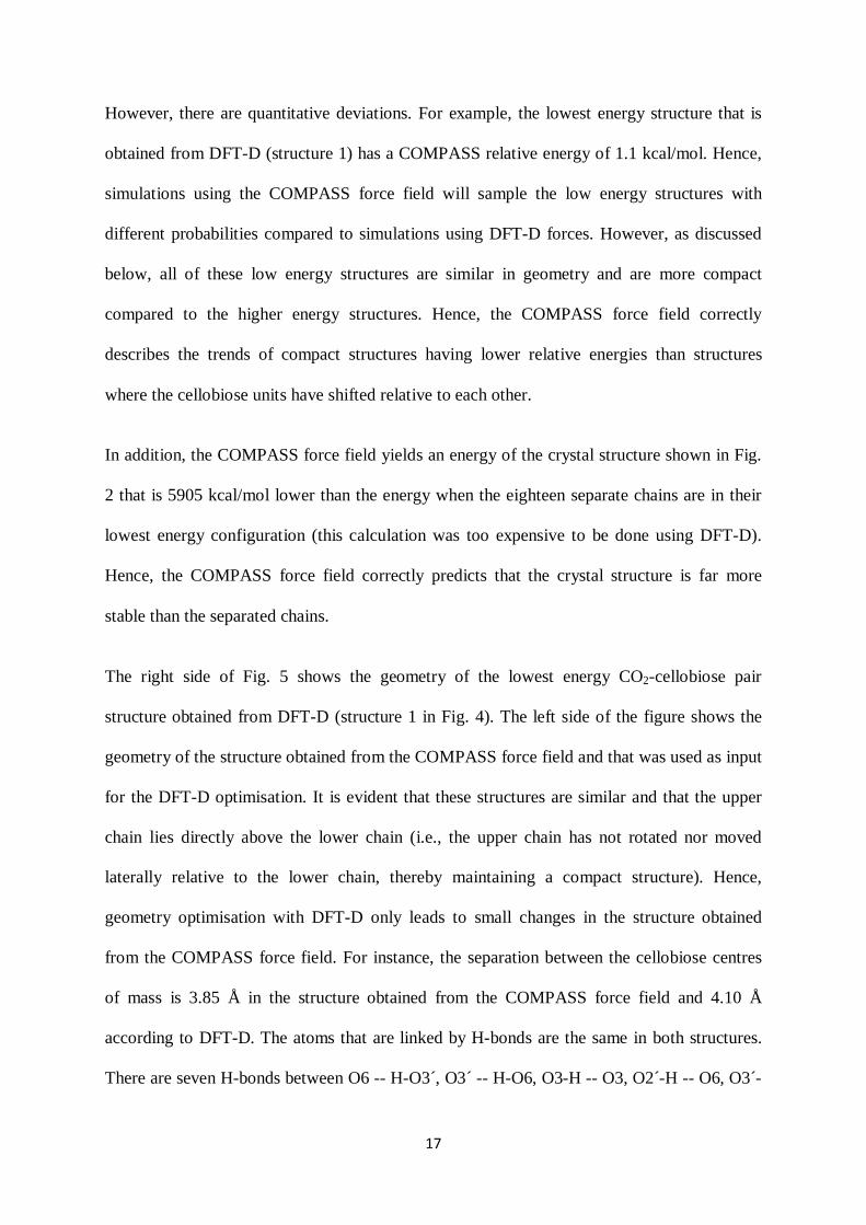
17

However, there are quantitative deviations. For example, the lowest energy structure that is

obtained from DFT-D (structure 1) has a COMPASS relative energy of 1.1 kcal/mol. Hence,

simulations using the COMPASS force field will sample the low energy structures with

different probabilities compared to simulations using DFT-D forces. However, as discussed

below, all of these low energy structures are similar in geometry and are more compact

compared to the higher energy structures. Hence, the COMPASS force field correctly

describes the trends of compact structures having lower relative energies than structures

where the cellobiose units have shifted relative to each other.

In addition, the COMPASS force field yields an energy of the crystal structure shown in Fig.

2 that is 5905 kcal/mol lower than the energy when the eighteen separate chains are in their

lowest energy configuration (this calculation was too expensive to be done using DFT-D).

Hence, the COMPASS force field correctly predicts that the crystal structure is far more

stable than the separated chains.

The right side of Fig. 5 shows the geometry of the lowest energy CO2-cellobiose pair

structure obtained from DFT-D (structure 1 in Fig. 4). The left side of the figure shows the

geometry of the structure obtained from the COMPASS force field and that was used as input

for the DFT-D optimisation. It is evident that these structures are similar and that the upper

chain lies directly above the lower chain (i.e., the upper chain has not rotated nor moved

laterally relative to the lower chain, thereby maintaining a compact structure). Hence,

geometry optimisation with DFT-D only leads to small changes in the structure obtained

from the COMPASS force field. For instance, the separation between the cellobiose centres

of mass is 3.85 Å in the structure obtained from the COMPASS force field and 4.10 Å

according to DFT-D. The atoms that are linked by H-bonds are the same in both structures.

There are seven H-bonds between O6 -- H-O3´, O3´ -- H-O6, O3-H -- O3, O2´-H -- O6, O3´-

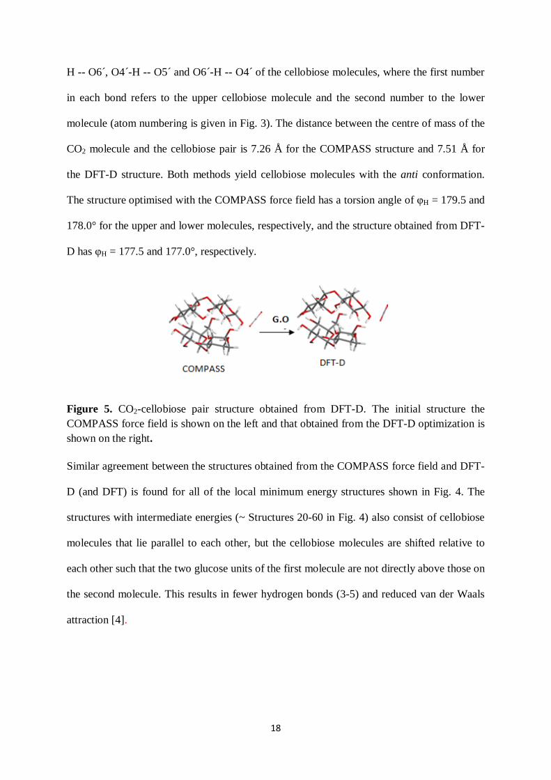
18

H -- O6´, O4´-H -- O5´ and O6´-H -- O4´ of the cellobiose molecules, where the first number

in each bond refers to the upper cellobiose molecule and the second number to the lower

molecule (atom numbering is given in Fig. 3). The distance between the centre of mass of the

CO2 molecule and the cellobiose pair is 7.26 Å for the COMPASS structure and 7.51 Å for

the DFT-D structure. Both methods yield cellobiose molecules with the anti conformation.

The structure optimised with the COMPASS force field has a torsion angle of φH = 179.5 and

178.0° for the upper and lower molecules, respectively, and the structure obtained from DFT-

D has φH = 177.5 and 177.0°, respectively.

Figure 5. CO2-cellobiose pair structure obtained from DFT-D. The initial structure the COMPASS force field is shown on the left and that obtained from the DFT-D optimization is shown on the right.

Similar agreement between the structures obtained from the COMPASS force field and DFT-

D (and DFT) is found for all of the local minimum energy structures shown in Fig. 4. The

structures with intermediate energies (~ Structures 20-60 in Fig. 4) also consist of cellobiose

molecules that lie parallel to each other, but the cellobiose molecules are shifted relative to

each other such that the two glucose units of the first molecule are not directly above those on

the second molecule. This results in fewer hydrogen bonds (3-5) and reduced van der Waals

attraction [4].

19

The cellobiose molecules in the structures with the highest energies have almost no overlap

of the glucose units. There are only 1 or 2 hydrogen bonds between the cellobiose molecules

in these structures.

Hence, the COMPASS force field correctly predicts that the crystal structure has lower

energy than the separated cellulose chains. Also, in agreement with DFT-D, the CO2

molecule does not lie between the cellobiose molecules, but is attached to the outer surface of

the cellobiose pair. In addition, both the COMPASS force field and DFT-D yield the same

trends in the relative energies of CO2-cellobiose pair structures. In the low energy structures

the cellobiose units are parallel to each other and have the two glucose units of one molecule

directly above those on the second molecule. This leads to a strong van der Waals attraction

and 6-7 H-bonds. Higher energy structure are less compact, since the cellobiose units are

shifted or rotated relative to each other, with a corresponding decrease in the number of H-

bonds. This indicates that the COMPASS force field provides a valid description for the

trends of CO2 interacting with cellulose and for the disruption of the cellulose crystal

structure. It was therefore used to study these trends during SC-CO2 explosion of cellulose.

3.2. Changes in the centre of mass during loading and explosion

Fig. 6 illustrates the changes in crystal structure after SC-CO2 explosion at 200 °C and 3500

psi. As illustrated by the small error bars presented below, all three trajectories integrated

under these conditions yielded similar changes in the crystal structure. The trends seen in the

figure are typical for all conditions studied here.

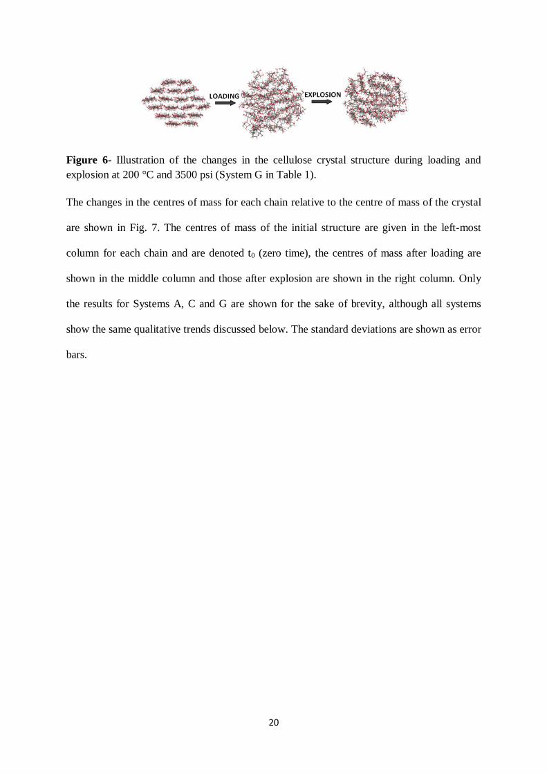
20

Figure 6- Illustration of the changes in the cellulose crystal structure during loading and explosion at 200 °C and 3500 psi (System G in Table 1).

The changes in the centres of mass for each chain relative to the centre of mass of the crystal

are shown in Fig. 7. The centres of mass of the initial structure are given in the left-most

column for each chain and are denoted t0 (zero time), the centres of mass after loading are

shown in the middle column and those after explosion are shown in the right column. Only

the results for Systems A, C and G are shown for the sake of brevity, although all systems

show the same qualitative trends discussed below. The standard deviations are shown as error

bars.

21

Figure 7- Centre of mass of each chain (1-18 in Fig. 2) relative to the centre of mass of the crystal for the initial structure (t0) and after loading and explosion. Results are for Systems A (110 °C/ 2500 psi), C (110 °C/ 3500 psi) and G (200 °C/ 3500 psi) and the standard deviations are from the three trajectories propagated at each temperature/ pressure combination.

Several features of the change in the crystal structure due to SC-CO2 loading and explosion

are revealed in Fig .7. First, the centres of mass of chains 3-5, 9-11, 15 and 18 decrease while

other chains show an increase in centres of mass relative to the centre of mass of the crystal.

Comparison with Fig. 2 shows that it is the chains on the left and right sides of the crystal that

have a decrease in centre of mass and the chains at the top and bottom of the crystal have an

0

9

18

1 2 3 4 5 6 7 8 9 10 11 12 13 14 15 16 17 18

A (110 °C/ 2500 psi)

0

9

18

1 2 3 4 5 6 7 8 9 10 11 12 13 14 15 16 17 18

C (110 °C/ 3500 psi)

CoM

(Å)

0

9

18

1 3 5 7 9 11 13 15 17

Chain No.

t0 Loading Explosion

G (200 °C/ 3500 psi)

t0

22

increase in centre of mass. This occurs since the pressure of the SC-CO2 make the crystal

structure more circular (this is also seen in Fig. 6).

Second, displacement of the chains in the outer layer (chains 1-12) is larger than chains in the

core. In addition, changes in the chains in the outer shell affect the displacement of their

neighbouring chains in the core. For example, during loading at 110 °C and 3500 psi, chains

1 and 7 move away from the centre of the crystal by about 4.3 and 3.9 Å, while chains 4 and

10 move closer to the centre about 2.7 and 2.1 Å. Similarly, chains 13 and 16, which

neighbour chains 1 and 7, respectively, move out by about 1.1 and 2.9 Å, respectively, while

chains 15 and 18 move inwards by about 0.7 Å.

Third, most of the changes occur during loading of the SC-CO2, and explosion has a far

smaller effect on the disruption of the structure (in fact, most of the changes occur during the

first picoseconds of the loading). For example, during loading at 110 °C and 3500 psi, the

absolute value of the change in centres of mass of chains 1-12 is, on average, 1.72 Å and for

the chains in the core (chains 13-18) it is 1.26 Å. This is larger than the changes during

explosion, which are 0.22 and 0.12 Å for the outer and core chains, respectively. Similarly, at

200 °C and 3500 psi the averages for chains 1-12 and 13-18 are 1.92 Å and 1.10 Å during

loading and 0.42 and 0.17 Å during explosion, respectively.

3.3. Effect of temperature and pressure

3.3.1. Temperature

The results in Fig. 7 showed that the centres of mass of chains 1, 6, 7 and 12 increased

relative to the centre of mass of the crystal, and that the centres of mass of chains 4, 5, 10

and 11 decreased. These two sets of chains are therefore grouped in the analysis presented

below for the sake of clarity. The left panel in Fig. 8 shows the effect of increasing

23

temperature on the average change in centre of mass of chains 1, 6, 7 and 12 after loading

and the combined loading and explosion. The pressure is 3500 psi and the temperature

increases from 110 to 200 °C (Systems C, E, F and G). The right panel is the same but for

chains 4, 5, 10 and 11.

Figure 8- Effect of temperature on the average of separation of centre of mass of chains 1, 6, 7 and 12 (left) and chains 4, 5, 10 and 11 (right) from the centre of mass of the crystal. The results are from loading and explosion at 3500 psi, for systems C (110 °C), E (135 °C), F (165 °C) and G (200 °C). The error bars are standard deviations obtained from the three trajectories propagated at each temperature/ pressure combination.

The results presented in the figure show that, although there is no significant effect of

increasing temperature (within the statistical uncertainty of the error bars), there is a trend of

increasing disruption of the crystal structure with increasing temperature. The average change

in the centres of mass of chains 1, 6, 7 and 12 when increasing from 110 to 135 °C is 0.35 Å,

and this increases to 0.48 and 1.11 Å with a further increase in temperature to 165 and 200

°C. Increasing the temperature has a smaller effect on the average centre of mass of chains 4,

5, 10 and 11, which is about 0.3 Å when the temperature increases from 110 to 200 °C.

Similarly to the discussion with reference to Fig. 7, Fig. 8 shows that explosion does not lead

to further disruption of the crystal structure. For example, explosion at 110, 135, 165 and 200

°C changes the average centres of mass of chains 1, 6, 7 and 12 by only about 0.14, 0.19,

0.05 and 0.48 Å (compared to the centres of mass after loading).

24

The results indicate that increasing the temperature helps to reduce the crystallinity of

cellulose, hence increasing accessibility to the hydrolysing enzymes. The largest effect is

during loading, and explosion may even cause slight agglomeration of the cellulose chains

(although the crystalline structure is not regained). It is possible that, for the materials used in

experimental SC-CO2 pretreatment, the explosion stage is needed to remove hemicellulose

and lignin that surrounds the cellulose crystal.

3.3.2. Pressure

Fig. 9 is the same as Fig. 8 but when the pressure is increased from 2500 to 4000 psi at a

constant temperature of 110 °C (Systems A, B, C and D). There is a larger change in

separation of the centre of mass of the chains relative to the centre of the crystal at lower

pressures. This is due to the fact that lower pressures allow chains 1, 6, 7 and 12 to move

further away from the centre of the crystal than at higher pressures. This, in turn, means that

chains 4, 5, 7 and 10 can move towards the centre of the crystal at the lower pressures. For

example, increasing the pressure from 2500 to 3000 psi during loading decreases the average

change in centre of mass separation for chains 1, 6, 7 and 12 by 0.48 Å. Further increases in

pressure to 3500 and 4000 psi leads to larger decreases of 0.78 and 1.27 Å compared to 2500

psi. Similarly, the average change in centre of mass separation for chains 4, 5, 7 and 10

differs by 0.8 Å between pressures of 2500 and 3000 psi, 1.1 Å between 2500 and 3500 psi

and 1.8 Å between 2500 and 4000 psi. Subsequent explosion shows no more disruption of

the crystal structure.

25

Figure 9- Same as for Fig. 8 but for systems A (2500 psi), B (3000 psi), C (3500 psi) and D (4000 psi). The temperature is 110 °C for all systems.

Fig. 9 shows that increasing the pressure at constant temperature leads to less disruption of

the cellulose crystal. This is in contradiction to some experiments [11, 12] that obtained

increased glucose yield with increasing pressure. However, it should be noted that these

experiments were performed with wet materials. Also, as discussed in the Introduction, this

may be due to the fact that the simulations consider crystalline cellulose, whereas the

lignocellulosic materials used in experiments typically contain other components such as

lignin and hemicellulose. Increasing the pressure may enhance disruption and removal of

these components, thereby and increasing the accessibility for the hydrolysing enzymes.

3.3.3. Effect of temperature and pressure on the separation of neighbouring cellulose chains

Fig. 10 shows the change in the separation of centres of mass of the non-reducing end, the O-

link in the centre of each chain and the reducing end between the outer chains and their

neighbouring core chains during loading and explosion. Only the data for systems C, D and G

are shown for the sake of brevity, and the trends seen in the figure are typical for all

conditions studied. The reason for choosing these three systems is to show the effect of high

temperature and high pressure on the separation of the different parts of neighbouring chains.

26

Figure 10- Change in the separation of centre of mass of the non-reducing end (Non-Red.), the O-link in the centre of each chain and reducing end (Red.) between the outer chains and their neighbouring inner chains during loading and explosion. The results are shown for loading and explosion at 110 °C and 3500 psi (System C), 110 °C and 4000 psi (System D) and 200 °C and 3500 psi (System G).

The figure reveals that there is a larger disruption at the ends of the chains than in the middle

(O-link) during both loading and explosion. Hence, there is larger disruption at the ends of

the crystal structure (i.e., at the chain ends) than in the middle of the crystal. This would lead

to enhanced accessibility for enzymatic hydrolysis at the crystal ends rather than in the

middle of the crystal.

The figure also shows that, similarly to the results presented above, increasing the pressure

has an insignificant effect on separation at the crystal ends whereas increasing the

temperature increases the separation between neighbouring chains. For example, the

separation between non-reducing ends of the outer chains and their inner neighbours,

averaged over all pairs, increases by ~0.74 Å when increasing the temperature from 110 to

200 °C. Increasing the pressure from 3500 to 4000 psi, leads to a change of only ~0.03 Å.

3.4. Correlation between the change in centre of mass of the cellulose chains and

their radii of gyration.

-1

0

1

2

non-

Red.

O-li

nk

Red.

non-

Red.

O-li

nk

Red.

non-

Red.

O-li

nk

Red.

110 °C, 3500 psi (C)

110 °C, 4000 psi (D)

200 °C, 3500 psi (G)

Chan

ge in

sep

arat

ion

(Å)

Loading Loading+ Explosion

27

No significant correlation was observed between the magnitude of the change in centres of

mass of chains during loading and explosion with changes in their radii of gyration. As an

example, Fig. 11 shows the change in radius of gyration for each chain as a function of its

change in centre of mass during explosion at 200 °C and 3500 psi (System G). The results are

typical for all initial structures and temperature/ pressure combinations. The lines shown in

the figure are best-fit straight lines to the chains in the outer shell (solid line) and the core

chains (dashed line). Although the solid line may indicate and increase in radius of gyration

with increasing change in centre of mass for the outer chains and the dashed line may indicate

the opposite trend for the core chains, these trends are not statistically meaningful since the

fits have R-squared values of 0.17 and 0.3 for the outer and core chains, respectively.

Figure 11- Change in radius of gyration for each chain as a function of its change in centre of mass during explosion at 200 °C and 3500 psi. The lines are best-fit straight lines to chains 1-12 in the outer shell (solid line) and the core chains 13-18 (dashed line).

3.5. Comparison with steam explosion

Similar studies have also been performed on steam explosion [58]. Comparison of the results

obtained here with those results show that the mechanism of crystal disruption during loading

and explosion is very similar for the water and CO2 solvents. For example, disruption occurs

mainly during loading and there is larger disruption at the cellulose crystal ends compared to

-0.4

-0.2

0

0.2

0.4

-1.4 -1.0 -0.6 -0.2 0.2 0.6

∆Ro

G

∆CoM

chains 1-12 chains 13-18Linear (chains 1-12) Linear (chains 13-18)

28

the central regions of the crystal, irrespective of which solvent is used. However, in general

the crystal disruption is larger during steam loading and explosion than SC-CO2 loading and

explosion. For example, the average change in the centres of mass of chains 1, 6, 7 and 12 is

4.28 and 3.76 Å when loading the system with steam at 250 °C and 576 psi and 210 °C and

275 psi, respectively. This can be compared to the value of 3.46 Å when loading the system

with SC-CO2 at 200 °C and 3500 psi (which, as shown in Fig. 8, yields the largest change).

Similarly, the average change in the separation between the non-reducing ends on

neighbouring outer and core chains is 2.57 Å for the steam explosion (250 °C and 576 psi)

and 1.14 Å for SC-CO2 at 200 °C and 3500 psi. As discussed above, the reason for the larger

changes seen in the steam loading and explosion is, at least partially, due to the lower

pressures and higher temperatures used in steam explosion (which is also the case in

experiments [19]).

4. Conclusion

First principles DFT-D, GCMC and MD methods have been used to study SC-CO2 loading

and explosion on the crystal structure of cellulose. This is the first step in a larger study of

SC-CO2 explosion of cellulosic waste, where other components such a lignin and

hemicellulose are present. SC-CO2 explosion of cellulosic waste is important since it is often

used in a pretreatment step for the conversion of this waste into biofuel. Insights gained from

molecular-level simulations are expected assist in improving the efficiency of this

pretreatment step as well as identifying new solvents or better processing conditions.

The GCMC and MD simulations were based on the COMPASS force field. This force field

yields the correct crystal structure for cellulose, and predicts that the crystal structure has

lower energy than the separated cellulose chains. Also, in agreement with DFT-D, studies

based on a system where a CO2 molecule interacts with a cellobiose pair, shows that the CO2

29

molecule does not lie between the cellobiose molecules, but is attached to the outer surface of

the cellobiose pair. Also, both the COMPASS force field and DFT-D yield the same trends in

the relative energies of CO2-cellobiose pair structures. In the low energy structures the

cellobiose units are parallel to each other and have the two glucose units of one molecule

directly above those on the second molecule. Higher energy structures are less compact, since

the cellobiose units are shifted or rotated relative to each other. This indicates that the

COMPASS force field provides a valid description for the trends of CO2 interacting with

cellulose and for the disruption of the cellulose crystal structure.

The GCMC and MD simulations show that most of the disruption of the crystalline structure

of cellulose occurs during loading of SC-CO2, and that explosion only has a small effect.

Disruption of cellulose chains in the outer crystal layer is larger than for chains in the core.

Also, separation between the non-reducing and reducing ends of neighbouring chains is

larger than the separation between the centres of these chains, showing that there is larger

distortion of the crystal structure at the ends of the crystal. Hence, these ends are more likely

to be accessible to enzyme attack than the central parts of the crystal. In addition, increasing

the temperature leads to a small increase in the disruption of the cellulose structure whereas

increasing the pressure decreases the disruption. There is no significant correlation between

the magnitude of the change in centres of mass of chains during loading and explosion and

their changes in their radii of gyration.

5. Acknowledgements

The authors acknowledge the Sparbanksstiftelsen Sjuhärad and the Carl Trygger Foundation

for Scientific Research for financial support. The molecular simulations were done using the

program from Accelrys Software Inc. GAMESS-US, version 1 OCT 2010 (R1) was used at

30

the high performance computer cluster Kalkyl at UPPMAX (Uppsala Multidisciplinary

Center for Advanced Computational Science), Uppsala Sweden.

31

References

1. Harmsen, P., et al., Literature review of physical and chemical pretreatment processes for lignocellulosic biomass. 2010: Wageningen UR, Food & Biobased Research.

2. Mamman, A.S., et al., Furfural: Hemicellulose/xylosederived biochemical. Biofuels, Bioproducts and Biorefining, 2008. 2(5): p. 438-454.

3. Ding, S.-Y. and M.E. Himmel, The maize primary cell wall microfibril: a new model derived from direct visualization. Journal of Agricultural and Food Chemistry, 2006. 54(3): p. 597-606.

4. Bazooyar F., B.M., Bolton K., Computational Studies of Water and Carbon Dioxide Interactions with Cellobiose. Journal of Molecular Modeling, 2014.

5. Eckert, C.A., Supercritical fluids as solvents for chemical and materials processing. Nature, 1996. 383: p. 313-318.

6. Kim, K.H. and J. Hong, Supercritical CO2 pretreatment of lignocellulose enhances enzymatic cellulose hydrolysis. Bioresource Technology, 2001. 77(2): p. 139-144.

7. Zheng, Y., et al., Supercritical carbon dioxide explosion as a pretreatment for cellulose hydrolysis. Biotechnology Letters, 1995. 17(8): p. 845-850.

8. Paljevac, M., et al., Hydrolysis of carboxymethyl cellulose catalyzed by cellulase immobilized on silica gels at low and high pressures. The Journal of Supercritical Fluids, 2007. 43(1): p. 74-80.

9. Gao, M., et al., Effect of SC-CO2 pretreatment in increasing rice straw biomass conversion. Biosystems engineering, 2010. 106(4): p. 470-475.

10. Canelas, D.A. and J.M. DeSimone, Polymerizations in liquid and supercritical carbon dioxide, in Metal Complex Catalysts Supercritical Fluid Polymerization Supramolecular Architecture. 1997, Springer. p. 103-140.

11. Zheng, Y., H. Lin, and G.T. Tsao, Pretreatment for cellulose hydrolysis by carbon dioxide explosion. 1998, Wiley Online Library. p. 890-896.

12. Narayanaswamy, N., et al., Supercritical carbon dioxide pretreatment of corn stover and switchgrass for lignocellulosic ethanol production, Elsevier. p. 6995-7000.

13. Gao, M., et al., Effect of SC-CO2 pretreatment in increasing rice straw biomass conversion, Elsevier. p. 470-475.

14. Ritter, D.C. and A.G. Campbell, Supercritical carbon dioxide extraction of southern pine and ponderosa pine. 1991, Soc Wood Sc Tech. p. 98-113.

15. Alvira, P., et al., Pretreatment technologies for an efficient bioethanol production process based on enzymatic hydrolysis: a review, Elsevier. p. 4851-4861.

32

16. Zheng, Y. and G.T. Tsao, Avicel hydrolysis by cellulase enzyme in supercritical CO2. 1996, Springer. p. 451-454.

17. Zheng, Y., et al., Supercritical carbon dioxide explosion as a pretreatment for cellulose hydrolysis. 1995, Springer. p. 845-850.

18. Alinia, R., et al., Pretreatment of wheat straw by supercritical CO2 and its enzymatic hydrolysis for sugar production, Elsevier. p. 61-66.

19. Gu, T., Pretreatment of lignocellulosic biomass using supercritical carbon dioxide as a green solvent, in Green Biomass Pretreatment for Biofuels Production, Springer. p. 107-125.

20. Luterbacher, J.S., J.W. Tester, and L.P. Walker, High-solids biphasic CO2 -H2O pretreatment of lignocellulosic biomass, Wiley Online Library. p. 451-460.

21. Kim, K.H. and J. Hong, Supercritical CO2 pretreatment of lignocellulose enhances enzymatic cellulose hydrolysis. 2001, Elsevier. p. 139-144.

22. Taherzadeh, M.J. and K. Karimi, Pretreatment of lignocellulosic wastes to improve ethanol and biogas production: a review. 2008, Molecular Diversity Preservation International. p. 1621-1651.

23. Stortz, C.A., et al., Comparison of different force fields for the study of disaccharides. 2009, Elsevier. p. 2217-2228.

24. Bergenstråhle, M., et al., Cellulose crystal structure and force fields, in International Conference on Nanotechnology for the forest products industry.

25. Ding, S.-Y. and M.E. Himmel, The maize primary cell wall microfibril: a new model derived from direct visualization. 2006, ACS Publications. p. 597-606.

26. Mazeau, K., Structural micro-heterogeneities of crystalline Iβ-cellulose. Cellulose, 2005. 12(4): p. 339-349.

27. Reiling, S. and J. Brickmann, Theoretical investigations on the structure and physical properties of cellulose. Macromolecular theory and simulations, 1995. 4(4): p. 725-743.

28. Neyertz, S., et al., A new all‐atom force field for crystalline cellulose I. Journal of applied polymer science, 2000. 78(11): p. 1939-1946.

29. Zhang, Q., et al., A molecular dynamics study of the thermal response of crystalline cellulose Iβ. Cellulose, 2011. 18(2): p. 207-221.

30. Bergenstråhle, M., L.A. Berglund, and K. Mazeau, Thermal response in crystalline Iβ cellulose: a molecular dynamics study. The Journal of Physical Chemistry B, 2007. 111(30): p. 9138-9145.

33

31. Sun, H., COMPASS: an ab initio force-field optimized for condensed-phase applications overview with details on alkane and benzene compounds. The Journal of Physical Chemistry B, 1998. 102(38): p. 7338-7364.

32. Bunte, S.W. and H. Sun, Molecular modeling of energetic materials: the parameterization and validation of nitrate esters in the COMPASS force field. The Journal of Physical Chemistry B, 2000. 104(11): p. 2477-2489.

33. Bunte, S.W. and H. Sun, Molecular modeling of energetic materials: the parameterization and validation of nitrate esters in the COMPASS force field. 2000, ACS Publications. p. 2477-2489.

34. Sun, H., COMPASS: an ab initio force-field optimized for condensed-phase applications overview with details on alkane and benzene compounds. 1998, ACS Publications. p. 7338-7364.

35. Aldred, P. Available from: P. Aldred, Atomistic modeling of the complex interactions of cellulose I and II polymorphs, http://www.accelrys.com/resource-center/case-studies /archive /studies /cellulose.html. Last downloaded: June 2014.

36. Sarko, A. and R. Muggli, Packing analysis of carbohydrates and polysaccharides. III. Valonia cellulose and cellulose II. Macromolecules, 1974. 7(4): p. 486-494.

37. Nishiyama, Y., P. Langan, and H. Chanzy, Crystal structure and hydrogen-bonding system in cellulose Iβ from synchrotron X-ray and neutron fiber diffraction. Journal of the American Chemical Society, 2002. 124(31): p. 9074-9082.

38. Kim, U.-J., S.H. Eom, and M. Wada, Thermal decomposition of native cellulose: influence on crystallite size. Polymer Degradation and Stability, 2010. 95(5): p. 778-781.

39. French, A.D. and G.P. Johnson, Advanced conformational energy surfaces for cellobiose**. Cellulose, 2004. 11(3-4): p. 449-462.

40. Becke, A.D., Density‐functional thermochemistry. III. The role of exact exchange. The Journal of Chemical Physics, 1993. 98(7): p. 5648-5652.

41. Lee, C., W. Yang, and R.G. Parr, Development of the Colle-Salvetti correlation-energy formula into a functional of the electron density. Physical Review B, 1988. 37(2): p. 785.

42. Miehlich, B., et al., Results obtained with the correlation energy density functionals of Becke and Lee, Yang and Parr. Chemical Physics Letters, 1989. 157(3): p. 200-206.

43. Momany, F.A. and J.L. Willett, Computational studies on carbohydrates: I. Density functional ab initio geometry optimization on maltose conformations. Journal of computational chemistry, 2000. 21(13): p. 1204-1219.

34

44. Lii, J.H., B. Ma, and N.L. Allinger, Importance of selecting proper basis set in quantum mechanical studies of potential energy surfaces of carbohydrates. Journal of computational chemistry, 1999. 20(15): p. 1593-1603.

45. Grimme, S., Accurate description of van der Waals complexes by density functional theory including empirical corrections. Journal of computational chemistry, 2004. 25(12): p. 1463-1473.

46. Piacenza, M. and S. Grimme, Van der Waals interactions in aromatic systems: structure and energetics of dimers and trimers of pyridine. ChemPhysChem, 2005. 6(8): p. 1554-1558.

47. Grimme, S., Semiempirical GGA‐type density functional constructed with a long‐range dispersion correction. Journal of computational chemistry, 2006. 27(15): p. 1787-1799.

48. Schmidt, M.W., et al., General atomic and molecular electronic structure system. Journal of Computational Chemistry, 1993. 14(11): p. 1347-1363.

49. Bolton, K. and S. Nordholm, An evaluation of the Gauss-Radau algorithm for the simulation of chemical dynamics. 1994, Elsevier. p. 320-335.

50. Fletcher, R. and C.M. Reeves, Function minimization by conjugate gradients. The computer journal, 1964. 7(2): p. 149-154.

51. Ermer, O., Calculation of molecular properties using force fields. Applications in organic chemistry, in Bonding forces. 1976, Springer. p. 161-211.

52. Levitt, M. and S. Lifson, Refinement of protein conformations using a macromolecular energy minimization procedure. Journal of molecular biology, 1969. 46(2): p. 269-279.

53. Nosé, S., A molecular dynamics method for simulations in the canonical ensemble. Molecular physics, 1984. 52(2): p. 255-268.

54. Nosé, S., A unified formulation of the constant temperature molecular dynamics methods. The Journal of Chemical Physics, 1984. 81(1): p. 511-519.

55. Shuichi, N., Constant temperature molecular dynamics methods. Progress of Theoretical Physics Supplement, 1991. 103: p. 1-46.

56. Erdtman, E., K.C. Satyanarayana, and K. Bolton, Simulation of α- and β-PVDF melting mechanisms. Polymer, 2012. 53(14): p. 2919-2926.

57. Strati, G.L., J.L. Willett, and F.A. Momany, Ab initio computational study of β-cellobiose conformers using B3LYP/6-311++ G**. Carbohydrate research, 2002. 337(20): p. 1833-1849.

58. Bolton, K., Bazooyar, F., Molecular-level Simulations of Cellulose Steam Explosion. Quantum Matter, 2014.