
Module 4 Energy performance assessment for Equipment and ...
169
c c ENERGY PERFORMANCE ASSESSMENT FOR EQUIPMENT AND UTILITY SYSTEMS Module 4 Sustainable and Renewable Energy Development Authority Power Division First Edition’2019
-
Upload
khangminh22 -
Category
Documents
-
view
1 -
download
0
Transcript of Module 4 Energy performance assessment for Equipment and ...

c
c
ENERGY
PERFORMANCE
ASSESSMENT
FOR
EQUIPMENT AND
UTILITY SYSTEMS
Module 4
Sustainable and Renewable Energy Development Authority
Power Division
First Edition’2019


Preamble
In order to ensure energy efficiency and conservation and to determine the future course of
action, Sustainable and Renewable Energy Development Authority (SREDA) has developed
the Energy Efficiency & Conservation Master Plan up to 2030 in 2016. According to this plan,
the target of energy saving has been set 15% & 20% per GDP by 2020 & 2030 respectively
which will be achieved by the use of energy efficient machinery and equipment as well as by
improving energy management system in the demand side .
In order to achieve the above mentioned target & to ensure the energy efficiency and
conservation in industrial & commercial sector, SREDA has formulated the Energy Audit
Regulation’2018. Based on this regulation, SREDA will conduct the Energy Auditor
Certification Examination to create energy auditors and energy managers in Bangladesh.
SREDA has prepared the following modules as reading material for four paper examinations
in cooperation with various National and Foreign partner organizations.
Module No Examination Paper Subject
Module 01 Paper 01 Fundamentals of Energy Management and Energy
Audit
Module 02 Paper 02 Energy Efficiency in Thermal Systems
Module 03 Paper 03 Energy Efficiency in Electrical Systems
Module 04 Paper 04 Energy Performance Assessment for Equipment and
Utility Systems
This module 04 on Energy Performance Assessment for Equipment and Utility Systems is the
reading material for the preparation of Paper 04 Examination for prospective candidates.
We hope that these modules will also act as valuable resource for practicing engineers in
comprehending and implementing energy efficiency measures in the facilities.
It is the first iteration of these modules. It will be a living document which can be reviewed
and revised time to time according to the evolution of the technology and industry. Any
suggestion and comments (please email to [email protected] ) on the contents of those
modules will be highly appreciated.


Table of Contents
Chapter 1: Compressed Air System .......................................................................................... 4
1.1 Introduction ..................................................................................................................... 4
1.2 Purpose of the Performance Test ................................................................................... 4
1.3 Performance Terms and Definitions .............................................................................. 4
1.4 Field Testing .................................................................................................................... 4
1.4.1 Measurement of free air by pump up test ................................................................ 4
1.4.2 Performance Assessment .......................................................................................... 5
Chapter 2: Lighting System .................................................................................................... 10
2.1 Introduction ................................................................................................................... 10
2.2 Purpose of the Performance Test ................................................................................. 10
2.3 Terms and Definitions ................................................................................................... 10
2.4 Preparation (before Measurements) ............................................................................. 11
2.5 Procedure of Assessment .............................................................................................. 11
2.5.1 Determine the Minimum Number and Positions of Measurement Points ............ 11
2.5.2 Calculation of the Installed Load Efficacy and Installed Load Efficacy Ratio of a
General Lighting Installation in an Interior .................................................................. 13
2.5.3 ILER Assessment .................................................................................................... 14
2.5.4 Sample Calculations ............................................................................................... 14
2.5.5 Areas of Improvement ............................................................................................ 15
Chapter 3: Fans and Blowers ................................................................................................. 16
3.1 Introduction ................................................................................................................... 16
3.2 Purpose of the Performance Test ................................................................................. 16
3.3 Performance Terms and Definitions ............................................................................ 16
3.4 Field Testing .................................................................................................................. 17
3.4 Factors that Could Affect Fan System Performance ............................................. 23
Chapter 4: Motors and Variable Speed Drives ...................................................................... 26
4.1 Introduction ................................................................................................................... 26
4.2 Terms and Definitions ................................................................................................... 26
4.2.1 Efficiency Testing ................................................................................................... 27
4.3 Determining Motor Loading ......................................................................................... 31
4.3.1 Input Power Measurements ................................................................................... 31
4.3.2 Line Current Measurements .................................................................................. 31
4.3.3 Slip Method ............................................................................................................. 32
4.4 Performance Evaluation of Rewound Motors ............................................................. 32

Module-4: Energy Performance Assessment for Equipment and Systems 1
4.5 Application of Variable Speed Drives (VSD) ............................................................... 34
4.5.1 Factors for Successful Implementation of Variable Speed Drives ....................... 35
4.5.2 Information needed to Evaluate Energy Savings for Variable Speed Application
.......................................................................................................................................... 37
Chapter 5: HVAC System ....................................................................................................... 39
5.1 Introduction ................................................................................................................... 39
5.2 Purpose of performance test ......................................................................................... 39
5.3 Terms and Definitions ................................................................................................... 39
5.4 Preparation for Measurements ..................................................................................... 39
5.5 Procedure ....................................................................................................................... 40
5.5.1 Performance evaluation of chilled water system ................................................... 40
5.5.2 Performance evaluation of air conditioning systems ............................................ 44
5.5.3 Procedure for Performance Evaluation of Vapour Absorption Refrigeration
(VAR) System ................................................................................................................... 50
5.5.4 Estimation of performance at evaporator side ...................................................... 50
5.5.5 Estimation of performance at condenser side (water cooled condenser) ............. 51
5.5.6 Performance assessment of Vapor Absorption Refrigeration (VAR) system: ..... 55
Chapter 6: Boiler Performance Assessment .......................................................................... 60
6.1 Introduction ................................................................................................................... 60
6.2 Purpose of the Performance Test ................................................................................. 60
6.3 Performance Terms and Definitions ............................................................................ 60
6.3.1 Direct method of testing ......................................................................................... 60
6.3.2 Measurements Required for Direct Method Testing ............................................. 61
6.3.3 Boiler Efficiency by Direct Method: Calculation and Example ........................... 62
6.3.4 The Indirect Method Testing .................................................................................. 63
6.3.5 Boiler Efficiency by Indirect Method: Calculation Procedure and Formula ...... 67
6.4 Efficiency for an oil fired boiler (Sample calculations) .............................................. 71
6.5 Factors Affecting Boiler Performance ......................................................................... 78
6.6 Data Collection Format for Boiler Performance Assessment ..................................... 79
6.6 Boiler Terminology ..................................................................................................... 80
Chapter 7: Cogeneration and Turbines (Gas, Steam) ........................................................... 86
7.1 Introduction ................................................................................................................... 86
7.2 Purpose of the Performance Test .................................................................................. 86
7.3 Field Testing Procedure ................................................................................................ 86
7.3.1 Test Duration........................................................................................................... 86
7.4 Measurements and Data Collection ............................................................................. 86
7.4.1 Thermal Energy ...................................................................................................... 87

Module-4: Energy Performance Assessment for Equipment and Systems 2
7.4.2 Electrical Energy .................................................................................................... 87
7.5 Performance Terms and Conditions............................................................................. 87
7.6 Calculations for Steam Turbine Cogeneration System ................................................ 88
Chapter 8: Pumping System ................................................................................................... 95
8.1 Introduction ................................................................................................................... 95
8.2 Purpose of the Performance Test .................................................................................. 95
8.4 Field Testing for Determination of Pump Efficiency .................................................. 96
8.4.1 Flow Measurement, Q ............................................................................................ 96
8.4.2 Determination of total head, H .............................................................................. 97
8.4.3 Determination of Hydraulic Power (Liquid Horse power) ................................... 98
8.4.4 Measurement of motor input power ....................................................................... 98
8.4.5 Pump shaft power ................................................................................................... 98
8.4.6 Pump Efficiency ..................................................................................................... 98
8.5 Pump Efficiency Calculation ........................................................................................ 98
8.6 Determining the System Resistance and Operating point (duty point) ....................... 99
Chapter 9: Heat Exchangers ................................................................................................ 103
9.1 Introduction ................................................................................................................. 103
9.2 Purpose of the Performance Test ................................................................................ 103
9.3 Performance Terms and Definitions .......................................................................... 103
9.3.1 Heat Duty .............................................................................................................. 103
9.3.2 Overall heat transfer coefficient, U ..................................................................... 104
9.3.3 Logarithmic Mean Temperature Difference (LMTD) ........................................ 104
9.3.4 The LMTD Correction Factor (F) ....................................................................... 105
9.3.5 Fouling Factor ...................................................................................................... 105
9.3.5 Effectiveness ......................................................................................................... 105
9.4 Methodology of Heat Exchanger Performance Assessment ..................................... 106
9.4.1 Procedure for determination of Overall Heat Transfer Coefficient, U atfield ... 106
9.4.3 Instruments for monitoring performance: .......................................................... 115
9.4.4 Terminology used in Heat Exchangers ............................................................... 115
Chapter 10: Financial Management .................................................................................... 119
10.1 Introduction ............................................................................................................... 119
10.2 Investment Need and Appraisal Criteria .................................................................. 119
10.2.1 Criteria ................................................................................................................ 120
10.3 Financial Analysis Approach and Techniques ........................................................ 121
10.3.1 Profit, Revenue and Costs .................................................................................. 121
10.3.2 Costs and Revenues ............................................................................................ 122

Module-4: Energy Performance Assessment for Equipment and Systems 3
10.3.3 Marginal analysis ............................................................................................... 123
10.3.4 Break-even Analysis: .......................................................................................... 124
10.4 Time Value of Money ................................................................................................ 125
10.4.1 How interest charges are calculated. ................................................................. 125
10.4.2 How to equate cash flows? ................................................................................. 126
10.4.3 Cost Escalation ................................................................................................... 128
10.4.4 Annuity ................................................................................................................ 129
10.5 Financial Analysis Techniques ................................................................................ 133
10.5.1 Simple Pay Back Period ..................................................................................... 133
10.5.2 Return on Investment (ROI) .............................................................................. 135
10.5.3 Benefit-Cost Analysis ......................................................................................... 136
10.5.4 Profitability index ............................................................................................... 136
10.6 Discounted Cash Flow Methods ............................................................................... 137
10.6.1 Net Present Value ............................................................................................... 137
10.6.2 Internal Rate of Return ...................................................................................... 141
10.6.3 Modified Internal Rate of Return ...................................................................... 144
Chapter 11: Sensitivity and Risk Analysis ........................................................................... 146
11.1 Impact of interest rates on cash flows ...................................................................... 147
11.2 Impact of Depreciation rates on cash flows ............................................................. 147
11.2.1 Straight-line Depreciation .................................................................................. 148
11.2.2 Reducing-balance Depreciation ......................................................................... 148
11.2.3 Sum of Years Depreciation ................................................................................. 149
11.2.4 Units of Production Depreciation ...................................................................... 150
11.3 Changes in inflation rates: Real value ..................................................................... 151
11.4 Considering Taxes in Financing and Investment .................................................... 152
11.5 Impact of taxes on cash flows ................................................................................... 154
11.6 Impact of Different Depreciation Methods and taxation on Cash flows ................ 154
Chapter 12: Financing Options ............................................................................................ 156
12.1 Energy Performance Contracting and Role of ESCOS ........................................... 156
12.1.1 What are performance contracts? ...................................................................... 157
12.2 Self-Financing Energy Management ....................................................................... 159
12.3 Ensuring Continuity .................................................................................................. 159

Module-4: Energy Performance Assessment for Equipment and Systems 4
Chapter 1: Compressed Air System
1.1 Introduction
The compressed air system is not only an energy intensive utility but also one of the least
energy efficient. Over a period of time, both performance of compressors and compressed air
system reduces drastically due to reasons such as poor maintenance, wear and tear etc. These
may lead to installing additional compressors causing more inefficiency. A periodic
performance assessment of compressor is essential to minimize the cost of compressed air.
1.2 Purpose of the Performance Test
To find out:
Actual Free Air Delivery (FAD) of the compressor
Specific power requirement
The actual performance of the plant is to be compared with design/standard values for assessing
the plant energy efficiency.
1.3 Performance Terms and Definitions
Free Air Delivery (FAD) Volume of air delivered under the conditions of
temperature and pressure at the compressor
suction
Specific Energy Consumption The ratio of power consumption (in kW) to the
volume delivered at ambient conditions
1.4 Field Testing
1.4.1 Measurement of free air by pump up test
Isolate the compressor along with its individual receiver from the main compressed air system
by tightly closing the isolation valve, thus closing the receiver outlet.
Open drain valve at the receiver to let out water and empty the receiver. Close the valve tightly
to start the test. Start the compressor and activate the stopwatch. Note the time taken to attain
the normal operational pressure P2 (in the receiver) from initial pressure P1.

Module-4: Energy Performance Assessment for Equipment and Systems 5
Calculate the capacity as per the following formula:
Actual Free air discharge
Free Air Delivery in m3/min is given by:
𝑄 =𝑃2 − 𝑃1
𝑃0𝑋
𝑉
𝑇 𝑁𝑚3/𝑚𝑖𝑛𝑢𝑡𝑒
Where
P2 = Final pressure after filling (kg/cm2 abs.)
P1 = Initial pressure (kg/cm2abs.) after bleeding
P0 = Atmospheric Pressure (kg/cm2 abs.)
V = Storage volume in m3 which includes receiver,
T
=
after cooler, and delivery piping
Time taken to build up pressure to P2 in minutes
The above equation is relevant where the compressed air temperature is same as the ambient
air temperature, i.e., perfect isothermal compression.
In case the actual compressed air temperature at discharge, say t20C is higher than ambient air
temperature say t1
0C (as is usual case),the FAD is to be corrected by a factor (273 + t1) / (273
+ t2).
1.4.2 Performance Assessment
Example 1.1
A plant has a compressor of rated capacity 1680 m3/hr. Free air delivery of the compressor is
carried out by filling the receiver.
The test data are as follows:
Receiver capacity : 10 m3
Interconnecting pipe : 1 m3
Initial pressure in receiver : 1.0 kg/cm2a
Inlet air pressure to compressor : 1.0 kg/cm2a
Final pressure : 8.25 kg/cm2a
Time taken to fill the receiver : 3 minutes (180 seconds)
Inlet air temperature : 30oC
Air temperature in the receiver : 40oC
Average duration of loading : 40 minutes in an hour
Average duration of unloading : 20 minutes in an hour
Power consumption during loading : 150 kW
Power consumption during unloading : 25 kW

Module-4: Energy Performance Assessment for Equipment and Systems 6
(a) Free Air Delivery in m3/min is given by:
(𝟖. 𝟐𝟓 − 𝟏) 𝑿 𝟏𝟏
𝟏 𝑿 𝟑 𝑿
(𝟐𝟕𝟑 + 𝟑𝟎)
(𝟐𝟕𝟑 + 𝟒𝟎)
: 25.73 m3/min
: 1545 m3/h
: 914 CFM
(b) % output when compared to rated capacity
: 1545/1680 x 100
: 92%
(c) Average Hourly air consumption:
Average duration of loading : 40 minutes in an hour
Average duration of unloading : 20 minutes in an hour
% loading of the compressor : 40 x 100/ (40+20)
: 66.7% loading
Hourly consumption of air is given by : % loading x actual output
: 0.667 x 1545
: 1030 m3/h
: 609 CFM
(d) Energy consumption:
% loading of the compressor : 66.7 %
% unloading of the compressor : 33.3 %
Hourly energy consumption is given by:
: (% loading x load power) + (% unloading x unload power)
: (0.667 x 150) + (0.333 x 25)
: 108.375 kWh
Daily energy consumption : 108.375 x 24
: 2601 kWh
(e) Overall Specific energy consumption (CFM/kW):
: Actual hourly air consumption in CFM
Hourly energy consumption
: 609/108.375
: 5.67 CFM/kW

Module-4: Energy Performance Assessment for Equipment and Systems 7
Example 1.2
A free air delivery test was carried out before conducting a leakage test on a reciprocating air
compressor in an engineering industry and following were the observations:
Receiver capacity : 8.0 m3
Initial pressure : 0.1 kg / cm2 gauge
Final pressure : 7.0 kg / cm2 gauge
Additional hold-up volume : 0.3 m3
Atmospheric pressure : 1.026 kg / cm2 abs.
Compressor pump-up time : 3.5 minutes
Further the following observations were made during the conduct of leakage test during the
lunch time when no pneumatic equipment/ control valves were in operation:
a) Compressor on load time is 24 seconds and unloading pressure is 7 kg/cm2gauage
b) Average power drawn by the compressor during loading is 92 kW
c) Compressor unload time and loading pressure are 79 seconds and 6.6kg/cm2 gauage
respectively.
Find out the following:
(i) Compressor output in m3/hr (neglect temperature correction)
(ii) Specific Power Consumption, kW/ m3/hr
(iii) % air leakage in the system
(iv) Leakage quantity in m3/hr
(v) Power lost due to leakage
(i) Compresser output m3/minute :
timePumpup Pressure Atm.
Volume Total PP 12
:
3.5 .0261
8.3 126.1026.8
= 15.948 m3/minute
: 956.89 m3/hr
(ii) Output : 956.89 m3/hr
Power consumption : 92 kW
Specific power consumption : 92/956.89 = 0.09614 kW/m3/hr
(iii) % Leakage in the system
Load time (T) : 24 s
Unload time (t) : 79 s
% leakage in the system : 100x)tT(
T

Module-4: Energy Performance Assessment for Equipment and Systems 8
:
100)7924(
24x
: 23.3%
iv) Leakage quantity : 0.233x956.89
: 222.955 m3/hr
v) Power lost due to leakage : Leakage quantity x specific power consumption
: 222.955 x 0.09614
: 21.43 kW
Example 1.3
An instrument air compressor capacity test gave the following results (assume the final
compressed air temperature is same as the ambient temperature) — Comment?
Solution:

Module-4: Energy Performance Assessment for Equipment and Systems 9
Example 1.4
In a medium sized engineering industry a 340 m3/hr reciprocating compressor is operated to
meet compressed air requirement at 7 bar. The compressor is in loaded condition for 80% of
the time. The compressor draws 32 kW during load and 7 kW during unload cycle.
After arresting the system leakages the loading time of the compressor came down to 60%.
Calculate the annual energy savings at 6000 hours of operation per year.
Solution:
Average power consumption with 80% loading = [0.8 x 32 + 0.2 x 7] = 27 kW
Average power consumption with 60% loading after leakage reduction = [0.6 x 32 + 0.4 x 7]
= 22 kW saving in electrical power = 5 KW
Yearly savings = 5 x 6000 = 30,000 kWH

Module-4: Energy Performance Assessment for Equipment and Systems 10
Chapter 2: Lighting System
2.1 Introduction
Lighting is provided in industries, commercial buildings, indoor and outdoor for providing
comfortable working environment. The primary objective is to provide the required lighting
level at lowest power consumption.
2.2 Purpose of the Performance Test
Most interior lighting requirements are for meeting average illuminance on a horizontal plane,
either throughout the interior, or in specific areas within the interior combined with general
lighting of lower illuminance.
The purpose of performance test is to calculate the installed efficacy in terms of lux/watt/m2
(existing or design) for general lighting installation. The calculated value can be compared with
the norms for specific types of interior installations for assessing improvement options. The
installed load efficacy of an existing (or design) lighting installation can be assessed by
carrying out a survey as indicated in the following sections.
2.3 Terms and Definitions
Lumen is a unit of light flow or luminous flux. The lumen rating of a lamp is a measure of the
total light output of the lamp. The most common measurement of light output (or luminous
flux) is the lumen. Light sources are labeled with an output rating in lumens.
Lux is the metric unit of measure for illuminance of a surface. One lux is equal to one lumen
per square meter.
Circuit Watts is the total power drawn by lamps and ballasts in a lighting circuit being assessed.
Installed Load Efficacy is the average maintained illuminance on a horizontal working plane
per circuit watt with general lighting of an interior. Unit: lux per watt per square metre
(lux/W/m2).
Lamp Circuit Efficacy is the amount of light (lumens) emitted by a lamp for each watt of power
consumed by the lamp circuit, i.e. including control gear losses. This is a more meaningful
measure for those lamps that require control gear. Unit: lumens per circuit watt (lm/W).
Average maintained illuminance is the average of lux levels measured at various points in a
defined area.
Color Rendering Index (CRI) is a measure of the effect of light on the perceived color of
objects. To determine the CRI of a lamp, the color appearances of a set of standard color chips
are measured with special equipment under a reference light source with the same correlated
color temperature as the lamp being evaluated. If the lamp renders the color of the chips
identical to the reference light source, its CRI is 100. If the color rendering differs from the
reference light source, the CRI is less than 100. A low CRI indicates that some colors may
appear unnatural when illuminated by the lamp.
Module-4: Energy Performance Assessment for Equipment and Systems 11
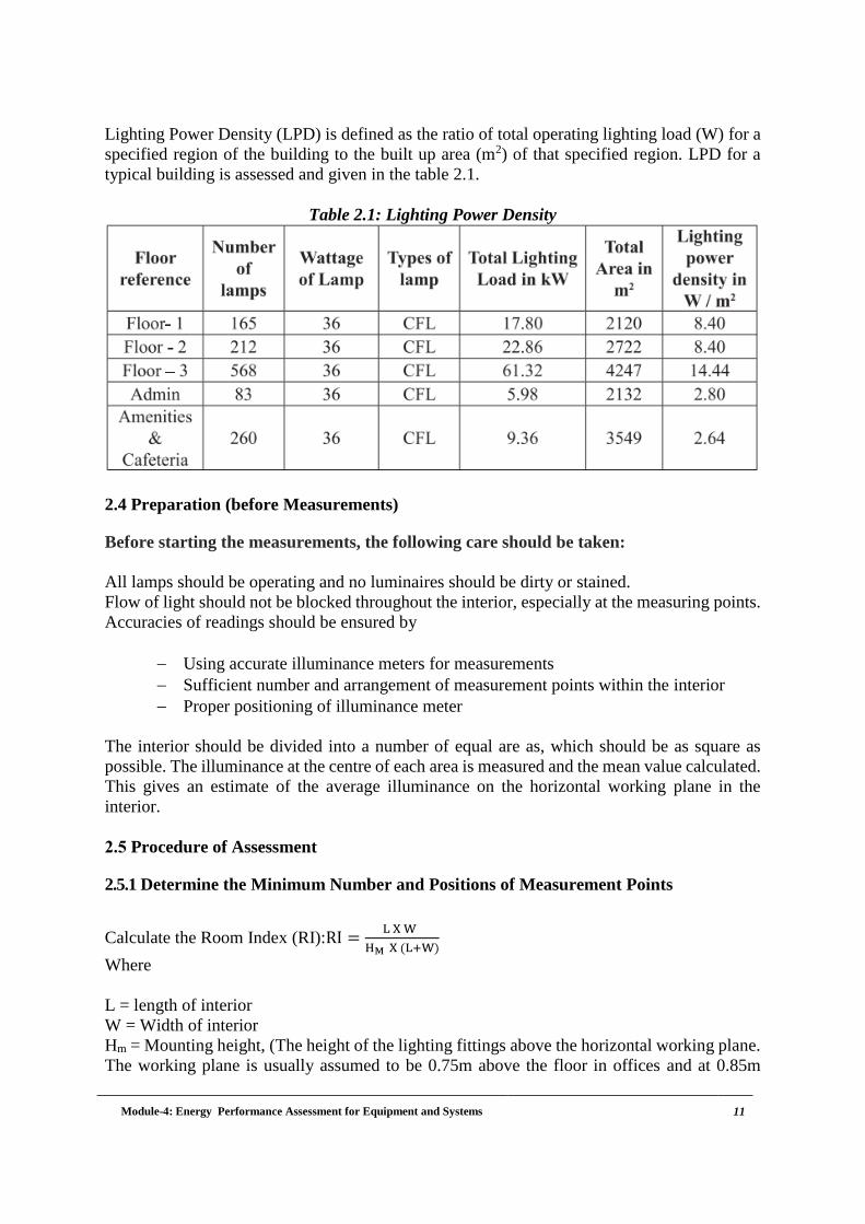
Lighting Power Density (LPD) is defined as the ratio of total operating lighting load (W) for a
specified region of the building to the built up area (m2) of that specified region. LPD for a
typical building is assessed and given in the table 2.1.
Table 2.1: Lighting Power Density
2.4 Preparation (before Measurements)
Before starting the measurements, the following care should be taken:
All lamps should be operating and no luminaires should be dirty or stained.
Flow of light should not be blocked throughout the interior, especially at the measuring points.
Accuracies of readings should be ensured by
Using accurate illuminance meters for measurements
Sufficient number and arrangement of measurement points within the interior
Proper positioning of illuminance meter
The interior should be divided into a number of equal are as, which should be as square as
possible. The illuminance at the centre of each area is measured and the mean value calculated.
This gives an estimate of the average illuminance on the horizontal working plane in the
interior.
2.5 Procedure of Assessment
2.5.1 Determine the Minimum Number and Positions of Measurement Points
Calculate the Room Index (RI):RI =L X W
HM X (L+W)
Where
L = length of interior
W = Width of interior
Hm = Mounting height, (The height of the lighting fittings above the horizontal working plane.
The working plane is usually assumed to be 0.75m above the floor in offices and at 0.85m

Module-4: Energy Performance Assessment for Equipment and Systems 12
above floor level in manufacturing areas.)
The minimum number of measurement points can be determined from Table 2.2.
Table 2.2: Determination of measurement points
Room Index Minimum number of
measurement points
Below 1 9
1 and below 2 16
2 and below 3 25
3 and above 36
For example, the dimensions of an interior are:
Length = 9m,
Width = 5m,
Height of luminaires above working plane (Hm) = 2m
RI= 9 x 5 / (2 x (9+5)) =1.607
From Table 2.2 the minimum number of measurement points is 16
As it is not possible to approximate a "square array" of 16 points within such a rectangle it is
necessary to increase the number of points to say 18, i.e. 6 x 3.
Therefore in this example the spacing between points along rows along the length of the interior
= 9 ÷ 6 = 1.5m and the distance of the 'end' points from the wall = 1.5 ÷ 2 = 0.75m.
Similarly the distance between points across the width of the interior = 5 ÷ 3 = 1.67m with half
this value, 0.83m, between the 'end' points and the walls.
Figure 2.1: Array of measuring points

Module-4: Energy Performance Assessment for Equipment and Systems 13
If the grid of the measurement points coincides with that of the lighting fittings, large errors
are possible and the number of measurement points should be increased to avoid such an
occurrence.
2.5.2 Calculation of the Installed Load Efficacy and Installed Load Efficacy Ratio of a
General Lighting Installation in an Interior
STEP 1 Measure the floor area of the interior: Area = m2
STEP 2 Calculate the Room Index: RI =
STEP 3 Determine the total circuit watts of the installation by a power
meter if a separate feeder for lighting is available:
(If the actual value is not known a reasonable approximation
can be obtained by totaling up the lamp wattages including the
ballasts)
Total circuit watts =
STEP 4 Calculate Watts per square metre:
(Value of step 3 ÷ value of step 1)
W/m2 =
STEP 5 Ascertain the average maintained illuminance by using lux
meter, Eav. Maintained:
Eav.maint. =
STEP 6 Divide 5 by 4 to calculate lux per watt per square Metre: Lux/W/m2 =
STEP 7 Obtain target Lux/W/m2 for type of the interior/application and
RI (2):
Target Lux/W/m2 =
STEP 8 Calculate Installed Load Efficacy Ratio (ILER) ( 6÷ 7 ): ILER =
Table 2.3: Target Values for Maintained illuminance on Horizontal Plane
The principal difference between the targets for Commercial and Industrial Ra: 40-85 (Cols.2

Module-4: Energy Performance Assessment for Equipment and Systems 14
& 3) of Table 2.3 is the provision for a slightly lower maintenance factor for the latter. The
targets for very clean industrial applications, with Ra: of 40 - 85, are as column2.
2.5.3 ILER Assessment
Compare the calculated ILER with the information in Table 2.4.
Table 2.4: Indicators of Performance
ILER Assessment
0.75 and above Satisfactory to Good
0.51 – 0.74 Review suggested
0.5 or less Urgent action required
ILER ratios of 0.75 and above are considered to be satisfactory. ILER ratios of 0.51 - 0.74 need
investigation to assess if improvements are possible. There may be reasons for a low ratio, such
as use of lower efficacy lamps or less efficient luminaires to achieve the required lighting
effects. In such cases, more efficient alternatives can be suggested. ILER ratio of 0.5 or less
certainly suggests scope for installation of more efficient lighting equipment.
After determining the ILER for the existing lighting installation, the difference between the
actual ILER and the best possible (1.0) can be calculated to estimate the energy wastage.
Annual Energy Wastage (in kWh) = (1.0 - ILER) x Total load (kW) x annual operating hours
(h)
2.5.4 Sample Calculations
STEP 1 Measure the floor area of the interior: Area = 45 m2
STEP 2 Calculate the Room Index RI = 1.93
STEP 3 Determine the total circuit watts of the installation by a power meter if a separate
feederforlightingisavailable.Iftheactualvalueisnotknownareasonableapproximat
ion can be obtained by totaling up the lamp wattages including the ballasts: Total
circuit watts = 990 W
STEP 4 Calculate Watts per square metre, 3 ÷1 : W/m2 = 22
STEP 5 Ascertain the average maintained illuminance, Eav. Maintained (average lux
levels measured at 18 points) Eav.maint. = 700
STEP 6 Divide 5 by 4 to calculate the actual lux per watt per square Metre Lux/W/m2 =
31.8
STEP 7 Obtain target Lux/W/m2for the type of interior/ application and RI (2):(Refer
Table 3) Target Lux/W/m2 = 46
STEP 8 Calculate Installed Load Efficacy Ratio (ILER) (6÷ 7). = 0.7
ILER of 0.7 means that there is scope for review of the lighting system as per Table 2.4.

Module-4: Energy Performance Assessment for Equipment and Systems 15
Annual energy loss = (1 - ILER) x watts x no. of operating hours
= (1 - 0.7) x 990 x 8 hrs/day x 300 days = 712 kWh/annum
2.5.5 Areas of Improvement
Identify natural lighting opportunities such as windows and other openings
For industrial lighting, explore the scope for introducing translucent sheets
Assess scope for more energy efficient lamps and luminaries
Assess scope for rearrangement of lighting fixtures

Module-4: Energy Performance Assessment for Equipment and Systems 16
Chapter 3: Fans and Blowers
3.1 Introduction
This section describes the method of testing a fan installed on site in order to determine the
performance of the fan in conjunction with the system to which it is connected.
3.2 Purpose of the Performance Test
The purposes of such ate stare to determine, under actual operating conditions, the flow rate,
the power input to the fan and the static pressure rise across the fan. These test results can be
compared with the value specified by supplier.
3.3 Performance Terms and Definitions
Static Pressure (PS): Static pressure is the amount of resistance measured in millimeter of water
column (mm WC).when air moves through a duct. It is the pressure exerted on the duct walls.
Velocity Pressure (PV): Velocity pressure is the pressure caused by air in motion. It is the
kinetic energy of a unit of air flow in an air stream. It is a function of air density and velocity
and it is used for determining air velocity in the duct.
Total Pressure (PT): The sum of static pressures and velocity pressures at a point.
Relationship between Velocity, total and
Static Pressures
PV = PT - PS
Where,
PV = Velocity Pressure
PT = Total Pressure
PS = Static Pressure
If velocity pressure is measured, velocity can
be calculated and air flow can be determined.
Figure 3.1
Fan Shaft Power: It is the mechanical power supplied to the fan shaft, also called as BHP.
Motor Input Power: The electrical power supplied to the terminals of an electric motor drive.

Module-4: Energy Performance Assessment for Equipment and Systems 17
Fan Static Efficiency:
Static, %
= Airflow in m3/s x P (Static Pressure) in mmWC
102 x Fan Shaft Power in kW
3.4 Field Testing
Instruction
Before site tests are carried out, it should be ensured that:
Fan and its associated equipment are functioning properly: no leakage
Operations are stable: steady temperature, static pressures, rated speed etc.
Measurement Locations
The flow measurement plane shall be located in any suitable straight length, (preferably on the
inlet side of the fan) where the airflow conditions are substantially axial, symmetrical and free
from turbulence.
The part of the duct where flow measurement plane is located should be straight, of uniform
cross-section and free from any obstructions which may modify the airflow.
For the purpose of determining the static pressure rise across the fan, the static pressure shall
be measured at planes on the inlet and outlet side of the fan sufficiently close to it.
Equivalent diameter (De).For rectangular duct, equivalent diameter, De is given by LW/ (L +
W) where L, W is the length and width of the duct. For circular ducts De is the same as diameter
of the duct.
Measurement of Air Velocity on Site
Velocity pressure is measured by pitot tube equipped with micro manometer (Figure 3.2). To
ensure accurate velocity pressure readings, the pitot tube tip must be pointed directly into
(parallel with) the air stream (Figure 3.3).
Pitot tube senses total and static pressure. Manometer measures velocity pressure (Difference
between total and static pressures) as shown in Figure 3.4.

Module-4: Energy Performance Assessment for Equipment and Systems 18
Figure 3.2: Pitot tube
Figure 3.3: Types of Pressure Measurement

Module-4: Energy Performance Assessment for Equipment and Systems 19
Figure 3.4: Pitot tube with Micromanometer
Traverse readings: The velocity of the air stream is not uniform across the cross section of a
duct. Friction slows the air moving close to the walls, so the velocity is greater in the center of
the duct.
To obtain the average velocity in ducts of 100mm diameter or larger, a series of velocity
pressure readings must be taken at points of equal area. A formal pattern of sensing points
across the duct cross section is recommended. These are known as traverse readings. Traverse
point location for circular duct is shown in Figure 3.5.
Figure 3.5 Traverse Points Location
Figure 3.6 shows recommended Pitot tube traverse point locations for traversing round and
rectangular ducts. In round ducts, velocity pressure readings should be taken at centers of equal
concentric areas.

Module-4: Energy Performance Assessment for Equipment and Systems 20
Figure 3.6: Pitot tube Traverse Point Location
The number of traverse points to be chosen depends upon the diameter in case of circular duct
and equivalent diameter in case of rectangular duct.
Example 3.1 Traverse point determination for round duct
Round duct:
Let us calculate various traverse points for a duct of 1 m diameter. From Figure6, for round
duct of 1 m (100 mm) diameter (D) and radius, R 0.5 m, 10 traverse points are chosen as
follows:
The various points from the port holes are given as follows:
0.5 – 0.949 x 0.5 0.0255
0.5 – 0.837 x 0.5 0.0815
0.5 – 0.707 x 0.5 0.1465
0.5 – 0.548 x 0.5 0.226
0.5 – 0.316 x 0.5 0.342
0.5 + 0.316 x 0.5 0.658
0.5 + 0.548 x 0.5 0.774
0.5 + 0.707 x 0.5 0.8535
0.5 + 0.837 x 0.5 0.9185
0.5 + 0.949 x 0.5 0.9745
Traverse point determination for rectangular duct (Sample Calculations)
Rectangular duct: For 1.4 m x 0.8 m rectangular duct, let us calculate the traverse points. 16
points are to be measured.

Module-4: Energy Performance Assessment for Equipment and Systems 21
Dividing the area 1.4 x 0.8 = 1.12 m2
into 16 equal areas, each area is 0.07 m2. Taking
dimensions of 0.35m x 0.20m per area, we can now mark the various points in the rectangular
duct as follows:
In very small ducts or where traverse operations are otherwise impossible, measurement can
be taken by placing Pitot tube in the centre of the duct.
Calculation of Velocity: After taking velocity pressures readings, at various traverse points, the
velocity corresponding to each point is calculated using the following expression.
Where,
Cp The pitot tube coefficient (take manufacturer’s value or assume 0.85)
Pv The velocity pressure measured using pitot tube and inclined manometer at each
point (traverse point) over the entire cross-section of the duct, mm water column
Gas density at flow conditions, kg/m3, corrected to normal temperature
Calculation of Density:
Where,
P – Absolute gas pressure, mmWC
M – Molecular weight of the gas, kg/kg mole (in the case of air M = 28.92 kg/kg mole)
R – Gas constant, 847.84 mmWC m3/kg mole K
T – Gas temperature, K
Calculation of Velocity and Flow rate:
Average velocity = V1 + V2+…VN
Total number of traverse points (N)
Where VN is the velocity at the Nth traverse point
v
p
p
81.92C (m/s)Velocity
TR
MPmkgDensity
3/),(

Module-4: Energy Performance Assessment for Equipment and Systems 22
Once the cross-sectional area of the duct is measured, the flow can be calculated as follows:
Airflow (Q), m3/s = Average velocity, V (m/s) x Fan duct area (m2)
Anemometer: The indicated velocity shall be measured at each traverse point in the cross
section by holding the anemometer stationary at each point for a period of time of not less than
1 minute. Each reading shall be converted to velocity in m/s and individually corrected in
accordance with the anemometer calibration. The arithmetic mean of the corrected point
velocities gives the average velocity in the air duct and the volume flow rate is obtained by
multiplying the area of the air duct by the average velocity.
Measurement of Static Pressure
The static pressure is measured at the inlet and outlet sides of the fan are taken relative to the
atmosphere pressure. This shall be done by using a U tube manometer or micro manometer in
conjunction with the static pressure connection of a pitot tube.
Determination of Power Input
Power Measurement: The power measurements can be best done using a suitable clamp- on
power meter.
Alternatively, if power meter is not available, by measuring the amps, voltage and assuming a
power factor of 0.9 the power can be calculated as follows:
P = √3 x V x I x cos
Transmission system between motor and fan involves losses. The following values shall be
used as a basis for transmission efficiency:
Properly lubricated precision spur gears 98% for each step
Flat belt drive 97%
V-belt drive 95%
If fan is driven by non-electric prime mover other than motor, fuel consumption (oil, steam,
compressed air etc.) should be specified and used in place of the motor power input.
Fan shaft power = Power input to the motor x of motor at the corresponding loading
x of transmission system
Fan static efficiency =Volume in
m3
sx Static pressure ascross the fan in mmWC
102 x fan shaft power

Module-4: Energy Performance Assessment for Equipment and Systems 23
Example 3.2
An energy audit of a fan was carried out. It was observed that the fan was delivering 18,500
Nm3/hr of air with static pressure rise of 45 mm WC. The power measurement of the motor
coupled with the fan recorded 8.7 kW. The motor operating efficiency was taken as 88%from
the motor performance curves. Assess the fan static efficiency.
Q = 18,500 Nm3/hr
= 5.13888 m3/sec
Static pressure rise across the fan, Pst = 45 mmWC
Power input to motor = 8.7 kW
=8.7 kW
Power input to fan shaft =8.7 x0.88=7.656 kW
Fan static = Volume in m3/sec x Pst in mmWc
102 x Power input to shaft
= 5.13888 x 45
102 x 7.656
= 0.296
= 29.6%
3.4 Factors that Could Affect Fan System Performance
Leakage, re-circulation or other defects in the system
Excessive loss in a system component located too close to the fan outlet
Disturbance of the fan performance due to a bender other system component located
too close to the fan inlet
Example 3.3
A fan handles 50,000 m3/hr of air at 90oC at static pressure difference of 70 mm WC. If the fan
static efficiency is 55%, find out the shaft power of the fan.
The plant proposes to cool the air from 90oC to 45oC before it enters the fan at an envisaged
static pressure difference of 60mmWC. What will be the power consumption of the fan after
cooling?
(a)
Q1 = 50,000 m3/hr,
P (static) = 70 mmWC
Fan Static Efficiency = 55%
Fan Power Pf1 = ?
Q1 = 50,000/3600
= 13.88 m3/sec
Fan Static Efficiency = Volume in m3 x P (static) in mm WC
102 x Power input to shaft in kW
Module-4: Energy Performance Assessment for Equipment and Systems 24
0.55 = (13.88 x 70 )/ 102 x Pf1
Shaft power drawn = 17.3 kW
(b)
Q1 = 50,000 m3/hr,
P2 (static) = 60 mmWC,
Fan Static Efficiency = 55%
Fan Power Pf2 = ?
Q2 = 50,000 x {(45 +273) / (90 +273)}
= 43,802 m3 / hr
= 43,802/3600 = 12.2 m3/sec
Fan Static Efficiency = Volume in m3 x P (static) in mm WC
102 x Power input to shaft in kW
0.55 = 12.2 x 60 / 102 x Pf2
Shaft power drawn = 13 kW
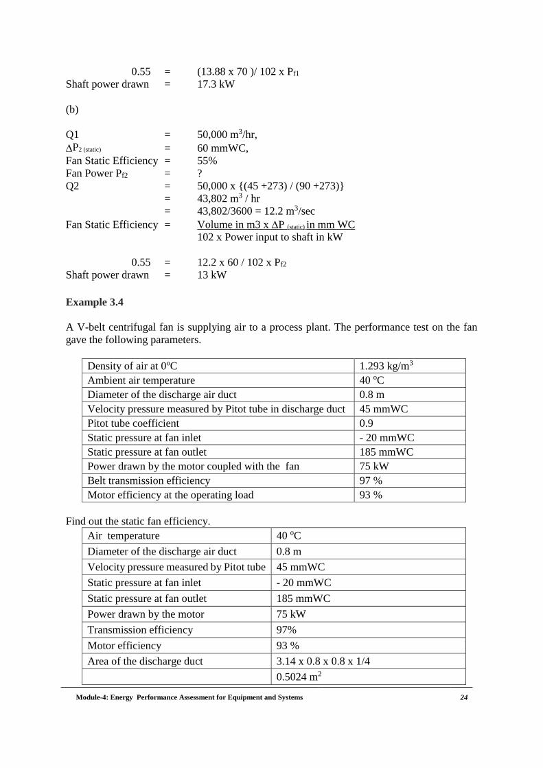
Example 3.4
A V-belt centrifugal fan is supplying air to a process plant. The performance test on the fan
gave the following parameters.
Density of air at 0oC 1.293 kg/m3
Ambient air temperature 40 oC
Diameter of the discharge air duct 0.8 m
Velocity pressure measured by Pitot tube in discharge duct 45 mmWC
Pitot tube coefficient 0.9
Static pressure at fan inlet - 20 mmWC
Static pressure at fan outlet 185 mmWC
Power drawn by the motor coupled with the fan 75 kW
Belt transmission efficiency 97 %
Motor efficiency at the operating load 93 %
Find out the static fan efficiency.
Air temperature 40 oC
Diameter of the discharge air duct 0.8 m
Velocity pressure measured by Pitot tube 45 mmWC
Static pressure at fan inlet - 20 mmWC
Static pressure at fan outlet 185 mmWC
Power drawn by the motor 75 kW
Transmission efficiency 97%
Motor efficiency 93 %
Area of the discharge duct 3.14 x 0.8 x 0.8 x 1/4
0.5024 m2

Module-4: Energy Performance Assessment for Equipment and Systems 25
Pitot tube coefficient 0.9
Corrected gas density (273 x 1.293) / (273 + 40) = 1.1277
Volume Cpx A (2 x 9.81 x p x )
0.9x0.5024x(2 x 9.81 x 45 x 1.1277)
1.1277
12.65 m3/s
Power input to the shaft 75 x 0.97 x 0.93
67.65 kW
Static fan efficiency =𝑉𝑜𝑙𝑢𝑚𝑒 𝑖𝑛
𝑚3
𝑠 𝑥 𝑡𝑜𝑡𝑎𝑙 𝑠𝑡𝑎𝑡𝑖𝑐 𝑝𝑟𝑠𝑠𝑢𝑟𝑒 𝑟𝑖𝑠𝑒 𝑖𝑛 𝑚𝑚𝑤𝑐
102 𝑥 𝑃𝑜𝑤𝑒𝑟 𝑖𝑛𝑝𝑢𝑡 𝑡𝑜 𝑡ℎ𝑒 𝑓𝑎𝑛 𝑠ℎ𝑎𝑓𝑡 𝑖𝑛 𝑘𝑊
Fan static Efficiency 12.65 x (185 – (–20)
102 x 67.65
37.58 %

Module-4: Energy Performance Assessment for Equipment and Systems 26
Chapter 4: Motors and Variable Speed Drives
4.1 Introduction
The two parameters of importance in a motor are efficiency and power factor. The efficiencies
of induction motors remain almost constant between 50 to 100% loading (refer Figure
4.1).When a motor has a higher rating than that required by the equipment, motor operates at
part load and the efficiency of them otoris reduced. Replacement o funder loaded motors with
smaller motors will allow a fully loaded smaller motor to operate at a higher efficiency. This
arrangement is generally most economical for larger motors, and only when they are operating
at less than one-third to one-half capacity.
Figure 4.1
4.2 Terms and Definitions
Efficiency: The efficiency of the motor is given by
=𝑃𝑜𝑢𝑡
𝑃𝑖𝑛= 1 −
𝑃𝐿𝑜𝑠𝑠
𝑃𝑖𝑛
Where
Pout – Output power of the motor
Pin – Input power of the motor
PLoss – Losses occurring in motor
Motor Loading: The motor loading, % is given by
Actual operating load of the motor
Rated capacity of the motor X 100

Module-4: Energy Performance Assessment for Equipment and Systems 27
4.2.1 Efficiency Testing
While input power measurements are fairly simple, measurement of output or losses need
laborious exercise with extensive testing facilities. The following are the testing standards
widely used.
Europe: IEC 60034-2, and the new IEC 61972
US: IEEE 112 - Method B
Japan: JEC 37
Even among these standards the difference in efficiency value is up to 3%.
For simplicity nameplate efficiency rating may be used for calculations if the motor load is in
the range of 50 -100 %.
Field Tests for Determining Efficiency
No Load Test:
The motorist unsaturated voltage and frequency without any shaft load. Input power, current
frequency and voltage are noted. The no load power factor (PF) is quite low and hence low PF
wattmeter’s are required.
From the input power, stator I2R losses under no load are subtracted to give the sum of friction,
wind age and core losses. To separate core and F & W losses, test is repeated at variable voltages
and no-load input kW versus voltage is plotted, the intercept is Friction & wind age (F&W)
loss component.
F&W and core losses = No load power (watts) – (No load current)2 x Stator resistance
Stator and Rotor I2R Losses:
The stator winding resistance is directly measured by a bridge or volt amp method. The
resistance must be corrected to the operating temperature. For modern motors, the operating
temperature is likely to be in the range of 1000C to 1200C and necessary correction should be
made. Correction to 750C may be inaccurate. The correction factor is given as follows:
𝑅2
𝑅1=
235 + 𝑡2
235 + 𝑡1
Where, t1 and t2 are ambient and operating temperature in °C respectively.
The rotor resistance can be determined from locked rotor test at reduced frequency, but rotor
I2R losses are measured from measurement of rotor slip.
Rotor I2R losses = Slip × (Stator Input – Stator I2R Losses – Core Loss)
Accurate measurement of slip is possible by stroboscope or non-contact type tachometer. Slip
also must be corrected to operating temperature.

Module-4: Energy Performance Assessment for Equipment and Systems 28
Stray Load Losses:
These losses are difficult to measure with any accuracy. IEEE Standard 112 gives a complicated
method, which is rarely used on shop floor. IS and IEC standards take a fixed value as 0.5% of
output. It must be remarked that actual value of stray losses is likely to be more. IEEE – 112
specifies values from 0.9 % to 1.8%.
Table 4.2
Motor Rating Stray Losses
1 – 125 HP 1.8 %
125 – 500 HP 1.5 %
501 – 2499 HP 1.2 %
2500 and above 0.9 %
Guidance for Users:
It must be clear that accurate determination of efficiency is very difficult. The same motor
tested by different methods and by same methods by different manufacturers can give a
difference of 2 %. In view of this, for selecting high efficiency motors, the following can be
done:
When purchasing large number of small motors or a large motor, ask for a detailed test
certificate. If possible, try to remain present during the tests. This will entail extra costs.
See that efficiency values are specified without any tolerance
Check the actual input current and kW, if replacement is done
For new motors, keep a record of no load input and current
Use values of efficiency for comparison and for confirming, rely on measured inputs
for all calculations.
Estimation of efficiency in the field can be done as follows:
Measure stator resistance and correct to operating temperature. From rated current
value, I2R losses are calculated.
From rated speed and output, rotor I2R losses are calculated
From no load test, core and F & W losses are determined for stray loss
The method is illustrated by the following example:
Example 4.1
Motor Specifications
Rated power
=
34 kW/45 HP
Voltage = 415 Volt

Module-4: Energy Performance Assessment for Equipment and Systems 29
Current = 57 Amps
Speed = 1475 rpm
Insulation class = F
Frame = LD 200 L
Connection = Delta
No load test Data
Voltage, V = 415 Volts
Current, I = 16.1 Amps
Frequency, F = 50 Hz
Stator phase resistance at 300C = 0.264 Ohms
No load power, Pnl = 1063.74 Watts
Calculate iron plus friction and wind age losses
Calculate stator resistance at1200C R2
R1=
235 + t2
235 + t1
Calculate stator copper losses at operating temperature of resistance at 1200C
Calculate full load slip(s) and rotor input assuming rotor losses are slip times rotor input.
Determine the motor input assuming that stray losses are 0.5 % of the motor rated power
Calculate motor full load efficiency and full load power factor
Solution
Iron plus friction and wind age loss, Pi = fw
Pnl = 1063.74Watts
Stator Copper loss, Pst-300C = 3 x (16.2/√3)2 ×0.264 = 68.43 Watts
Pi+fw =Pnl –Pst –Cu =1063.74 – 68.43 = 995.3 Watts
Stator Resistance at1200C,
R1200C = 0.264 × (120 + 235/ 30+235) = 0.354 ohms
Stator copper losses at full load,
Pst - Cu-1200C =3×(57/√3)2 ×0.354 = 1150.1 Watts

Module-4: Energy Performance Assessment for Equipment and Systems 30
Full load slip
S = (1500 – 1475) / 1500 = 0.0167
Rotor input, Pr = Poutput/(1-S) = 34000 / (1- 0.0167) = 34577.4 Watts
Motor full load input power, Pinput
= Pr +Pst –Cu–1200C+Pi +fw+Pstray = 34577.4 + 1150.1 + 995.3 + (0.005 × 34000)
= 36892.8 Watts
Motor efficiency at full load
Comments:
a) The measurement of stray load losses is very difficult and not practical even on test
beds.
b) The actual value of stray loss of motors up to 200 HP is likely to be 1 % to 3 %
compared to 0.5 % assumed by standards.
c) The value of full load slip taken from the nameplate data is not accurate. Actual
measurement under full load conditions will give better results.
d) The friction and wind age losses really are part of the shaft output; however, in the
above calculation, it is not added to the rated shaft output, before calculating the rotor
input power. The error however is minor.
e) When a motorist rewound, there is a fair chance that the resistance per phase would
increase due to winding material quality and the losses would be higher. It would be
interesting to assess the effect of a nominal 10 % increase in resistance per phase.

Module-4: Energy Performance Assessment for Equipment and Systems 31
4.3 Determining Motor Loading
4.3.1 Input Power Measurements
First measure input power Pi with a hand held or in-line power meter Pi = Three-phase
power in kW
Note the rated kW and efficiency from the motor name plate
The figures of kW mentioned in the name plate are for output conditions. So
corresponding input power at full-rated load
Pir =Name plate full rated kW
𝒇𝒍
Where,
ηfl= Efficiency at full-rated load
Pir= Input power at full-rated load in kW
The percentage loading can now be calculated as follows
% 𝑳𝒐𝒂𝒅𝒊𝒏𝒈 =𝑷𝒊
𝑷𝑰𝒓𝑿 𝟏𝟎𝟎%
Example 4.2
The name plate details of a motor are given as power = 15 kW, efficiency, η = 0.9. Using a
power meter the actual three phase power drawn is found to be 8 kW. Find out the loading of
the motor.
Input power at full-rated power in kW, Pir = 15 /0.9 = 16.7 kW
Percentage loading = 8/16.7 = 48%
4.3.2 Line Current Measurements
The line current load estimation method is used when input power cannot be measured and
only amperage measurements are possible. The amperage draw of a motor varies approximately
linearly with respect to load, down to about 75% of full load. Below the 75% load point, power
factor degrades and the amperage curve becomes increasingly non-linear.
In the low load region, current measurements are not a useful indicator of load. However, this
method may be used only as a preliminary method just for the purpose of identification of
oversized motors.
% Load =Input load current
Input rated current x 100 (valid up to 75% loading)

Module-4: Energy Performance Assessment for Equipment and Systems 32
4.3.3 Slip Method
In the absence of a power meter, the slip method can be used which requires a tachometer. This
method also does not give the exact loading on the motors.
Load =Slip
SS − Sr x 100%
Where:
Load = Output power as a % of rated power
Slip = Synchronous speed - Measured speed in rpm
Ss = Synchronous speed in rpm at the operating frequency
Sr = Nameplate full-load speed
Example 4.3 Slip Load Calculation
Slip also varies inversely with respect to the motor terminal voltage squared. A voltage
correction factor can, also, be inserted into the slip load equation. The voltage compensated
load can be calculated as shown
Load =Slip
(SS − Sr) x (Vr/V)2 x 100%
Where:
Load = Output power as a % of rated power
Slip = Synchronous speed - Measured speed in rpm
Ss = Synchronous speed in rpm
Sr = Nameplate full-load speed
V = RMS voltage, mean line to line of 3 phases
Vr= Nameplate rated voltage
4.4 Performance Evaluation of Rewound Motors
Ideally, a comparison should be made of the efficiency before and after a rewinding. A
relatively simple procedure for evaluating rewind quality is to keep a log of no-load input
current for each motor in the population. This figure increases with poor quality rewinds. A
review of the rewind shop's procedure should also provide some indication of the quality of
work. When rewinding a motor, if smaller diameter wire is used, the resistance and theI2R
losses will increase.

Module-4: Energy Performance Assessment for Equipment and Systems 33
The motor loading survey can be performed using the format given below:
Table 4.3: Motor Field Measurement Format
The monitoring format for rewound motor is given below:
Table 4.4: Monitoring format for rewound motor

Module-4: Energy Performance Assessment for Equipment and Systems 34
4.5 Application of Variable Speed Drives (VSD)
Although there are many methods of varying the speeds of the driven equipment such as
hydraulic coupling, gearbox, variable pulley etc., the most possible method is varying the
motor speed by varying the frequency and voltage by using a variable frequency drive.
RPM = (f x 120) / p
Where f is the frequency in Hz, and p is the number of poles in any multiple of 2.
Therefore, if the frequency applied to the motor is changed, the motor speed changes in direct
proportion to the frequency change. The control of frequency applied to the motor is the job
given to the VSD.
The VSD's basic principle of operation is to convert the electrical system frequency and voltage
to the frequency and voltage required to drive a motor at a speed other than its rated speed. The
two most basic functions of a VSD are to provide power conversion from one frequency to
another, and to enable control of the output frequency.
VFD Power Conversion
As illustrated by Figure 4.3, there are two basic components, a rectifier and an inverter for
power conversion. The rectifier receives the 50-HzAC voltage and converts it to direct current
(DC) voltage. A DC bus inside the VSD functions as a "parking lot "for the DC voltage. The
DC bus energizes the inverter, which converts it back to AC voltage again. The inverter can be
controlled to produce an output frequency of the proper value for the desired motor shaft speed.
Figure 4.2: VFD Power Converter

Module-4: Energy Performance Assessment for Equipment and Systems 35
4.5.1 Factors for Successful Implementation of Variable Speed Drives
Load Type for Variable Frequency Drives
The main consideration is whether the variable frequency drive application requires a variable
torque or constant torque drive.
If the equipment being driven is centrifugal, such as a fan or pump, then a variable torque drive
will be more appropriate. A fan needs less torque when running at 50% speed than it does when
running at full speed. Variable torque operation allows the motor to apply only the torque
needed, which results in significant reduction in energy consumption.
Conveyors, positive displacement pumps, punch presses, extruders, and other similar type
applications require constant level of torque at all speeds. In which case, constant torque
variable frequency drives would be more appropriate for the job. A constant torque drive
should have an overload current capacity of 150% or more for one minute. Variable torque
variable frequency drives need only an overload current capacity of 120% for one minute since
centrifugal applications rarely exceed the rated current.
If tight process control is needed, then you may need to utilize a sensor less vector, or flux
vector variable frequency drive, which allow a high level of accuracy in controlling speed,
torque, and positioning.
Motor Information
The following motor information will be needed to select the proper variable frequency drive:
Full Load Amperage Rating: Using a motor's horse power is an inaccurate way to size variable
frequency drive.
Speed Range: Generally, a motor should not be run at any speed less than 20% of its specified
maximum speed allowed. If it is run at a speed less than this without auxiliary motor cooling,
the motor will over heat. Auxiliary motor cooling should be used if the motor must be operated
at very slow speeds.
Multiple Motors: To size a variable frequency drive that will control more than one motor, add
to get her the full-load amp ratings of each of the motors. All motors controlled by a single
drive must have an equal voltage rating.
Efficiency and Power Factor
The variable frequency drive should have an efficiency rating of 95% or better at full load.
Variable frequency drives should also offer a true system power factor of 0.95 or better across
the operational speed range, to save on demand charges, and to protect the equipment
(especially motors).

Module-4: Energy Performance Assessment for Equipment and Systems 36
Protection and Power Quality
Motor overload Protection for instantaneous trip and motor over current.
Additional Protection: Over and under voltage, over temperature, ground fault, and control or
microprocessor fault. These protective circuits should provide an orderly shutdown of the VFD,
provide indication of the fault condition, and require a manual reset (except under voltage)
before restart. Under voltage from a power loss shall be set to automatically restart after return
to normal. The history of the previous three faults shall remain in memory for future review.
If a built-up system is required, there should also be externally-operated short circuit
protection, door-interlocked fused disconnect and circuit breaker or motor circuit protector
(MCP)
To determine if the equipment under consideration is the right choice for a variable speed drive
application:
The load patterns should be thoroughly studied before exercising the option of VSD. In effect
the load should be of a varying nature to demand a VSD (refer Figures 4.3 and 4.4).
The first step is to identify the number of operating hours of the equipment at various load
conditions. This can be done by using a Power analyzer with continuous data storage or by a
simple energy meter with periodic reading being taken.
Example 4.4
Operating boiler load and associated induced draft fan-power consumption of a boiler is given
as follows:
Boiler loading
(%)
Damper
position
Operating
hours/day
Fan-motor power with damper
operation (kW)
100 Full open - 35
80 Position #1 4 31
70 Position #2 12 29
60 Position #3 8 26
Figure 4.3: Load pattern Figure 4.4: Load pattern

Module-4: Energy Performance Assessment for Equipment and Systems 37
Estimate the daily energy savings that can be achieved if the damper is replaced by a VFD for
induced draft fan to meet the desired requirements. Assume that the air requirement is
proportional to boiler loading.
Fan flow
(proportional
to boiler
loading)
Operating
hrs/day
Fan-motor
power with
damper (kW)
Fan-motor
with VFD
(kW)
Power
savings
(kW)
Energy
savings
(kWh)
A B C D = A3 x 35 E=CD F=B x E
80 4 31 0.83 x 35 =
17.9
13.1 52.32
70 12 29 0.73 x 35 = 12 17 203.94
60 8 26 0.63 x 35 = 7.6 18.4 147.52
Total daily energy savings 403.78
4.5.2 Information needed to Evaluate Energy Savings for Variable Speed Application
Method of flow control to which adjustable speed is compared:
• output throttling (pump) or dampers (fan)
• recirculation (pump) or unrestrained flow (fan)
• adjustable-speed coupling (eddy current coupling)
• inlet guide vanes or inlet dampers (fan only)
• two-speed motor.
Pump or fan data:
• head v's flow curve for every different type of liquid (pump) or gas (fan) that
is handled
• Pump efficiency curves.
Process information:
• specific gravity (for pumps) or specific density of products (for fans)
• system resistance head/flow curve
• equipment duty cycle, i.e. flow levels and time duration.
Efficiency information on all relevant electrical system apparatus:
• motors, constant and variable speed
• variable speed drives
• gears
• transformers.
If we do not have precise information for all of the above, we can make reasonable assumptions
for points 2 and 4.
Example 4.5
a) In a 75 kW four pole induction motor operating at 49.8 Hz and rated for 415 V and 1440
RPM, the actual measured speed is 1470 RPM. Find out the percentage loading of the motor if
the voltage applied is 428 V.
b) A 6 pole, 415 volt, 3 (13, 50 Hz induction motor delivers 22 kW power at rotor shaft at a
speed of 950 rpm with PF of 0.88. The total loss in the stator including core, copper and other
losses is 2 kW. Calculate the following. i) Slip ii) Rotor Copper Loss iii) Total Input to motor

Module-4: Energy Performance Assessment for Equipment and Systems 38
iv) Line current at 415 V and motor pi of 0.88 v) Motor operating efficiency
Solution:

Module-4: Energy Performance Assessment for Equipment and Systems 39
Chapter 5: HVAC System
5.1 Introduction
Air conditioning and refrigeration consume significant amount of energy in buildings and in
process industries. The energy consumed in air conditioning and refrigeration systems depends
on load changes, seasonal variations, operation and maintenance, ambient
conditionsetc.Hencetheperformanceevaluationwillhavetotakeintoaccounttotheextent possible
all these factors.
5.2 Purpose of performance test
The purpose of performance assessment is to verify the performance of a refrigeration system
by using field measurements. The test will measure net cooling capacity (tons of refrigeration)
and energy requirements, at the actual operating conditions. The objective of the test is to
estimate the energy consumption at actual load as against design conditions.
5.3 Terms and Definitions
Refrigeration Capacity: Refrigeration Capacity is stated in terms of Tons of Refrigeration
(TR). One TR is the amount of heat to be removed (3024 kcal/hr) from the atmosphere to melt
one metric (short) ton of pure ice at 0 °C in 24 hours.
1 TR = 3024 kCal/h = 12000 Btu/h = 3.517 kW
Specific Power Consumption (kW/TR): It is the ratio of power input to compressor motor (kW)
over tons of refrigeration (TR) produced. Lower kW/TR indicates higher efficiency.
Coefficient of Performance (COP): It is the ratio of refrigeration capacity (cooling capacity)
and input power (kW) to chiller compressor. Higher COP indicates better performance.
Energy Efficiency Ratio (EER): Performance of smaller chillers and rooftop units is frequently
stated as EER rather than kW/TR.EER is calculated by dividing the chiller cooling capacity (in
Btu/h) by its power input (in watts) at full-load conditions. The higher the EER, the more
efficient is the unit.
5.4 Preparation for Measurements
The reading should be taken after steady-state conditions are established. To minimize the
effects of transient conditions, test readings should be taken simultaneously as possible.
Minimum of three sets of data shall be taken, at a minimum of five-minute intervals.

Module-4: Energy Performance Assessment for Equipment and Systems 40
5.5 Procedure
5.5.1 Performance evaluation of chilled water system
Net refrigeration capacity
The test shall include a measurement of the net heat removed from the water as it passes
through the evaporator by measuring the following:
• Chilled water flow rates
• Temperature of chilled water entering the evaporator
• Temperature of chilled water leaving the evaporator
• Evaporator water pressure drop (across inlet and outlet)
All instruments, including gauges and thermometers shall be calibrated over the range of test
readings for the measurement of following parameters.
Methods of measuring the chilled water flow rate
In the absence of an on-line flow meter, the chilled water flow can be measured by the
following methods
• In case where hot well and cold well are available, the flow can be measured from the
tank level fall (dip) or rise by switching off the secondary pump.
• Non-invasive method would require a well calibrated ultrasonic flow meter using which
the flow can be measured without disturbing the system
• If the waterside pressure drop is close to the design values, it can be assumed that the
water flow of pump is same as the design rated flow.
Net refrigeration capacity (Refrigeration capacity in tons of refrigeration, TR) is determined
by calculating the product of the chilled water flow rate, the chilled water temperature
difference across the evaporator, and the specific heat of the water.
Net Refigeration Capacity, TR = QCH x dW x CP x ( Ti − TO)
3024
Where,
QCH - Flow rate of chilled water in m3/hr
dW - Density of water, kg/m3
CP - Specific heat of water in kcal/kg oC
TI - Inlet (supply) temperature of chilled water to evaporator in oC
TO - Outlet (return) temperature of chilled water from evaporator (chiller) in oC
The same equation can be used if any other liquid is used instead of chilled water, only density
of the liquid should be known. The temperature measurement should be accurate and least count
should be at least one decimal should be ensured.

Module-4: Energy Performance Assessment for Equipment and Systems 41
Measurement of compressor power
The compressor input power can be measured by a portable power analyser which would give
reading directly in kW.
Alternatively, the ampere can be measured by the available on-line ammeter or by using a tong
tester. The power can then be calculated by assuming a power factor of 0.9.
Input power (kW) = √3 x V x I x Cos
To determine the heat rejected at the condenser
Heat rejected at condenser = Cooling load + Work done by compressor
The shaft power kW absorbed (work done) by the compressor can be derived by measuring the
motor input power multiplied by motor operating efficiency.
Heat rejected at the condenser can be measured as under:
Water cooled condenser:
a. Measure the water quantity flowing through the condenser using flow meter.
b. Measure the inlet and outlet temperature of water in the condenser using digital thermometer.
Mc - Mass flow rate of cooling water, kg/h
Cp - Specific heat of water, kcal/kg°C
twi - Cooling water temperature at condenser inlet, °C
two - Cooling water temperature at condenser outlet, °C
Air cooled condenser:
a. Measure the air quantity flowing across condenser coil.
b. Measure the inlet and outlet temperatures of air using digital thermometer.
Since this process is normally a sensible heating, the capacity can be established by calculating
only sensible heat gain.

Module-4: Energy Performance Assessment for Equipment and Systems 42
Where,
Ma - Mass flow rate of air, kg/h
Cpa - Specific heat of air, kcal/kg°C
ta i- Temperature of cooling air at condenser inlet °C tx,
tao - Temperature of cooling air at condenser outlet °C
Measurement of air flow
Air flow may be measured with any of the following instruments:
a) Vane Anemometer
b) Hot wire anemometer
The measuring instruments should be duly calibrated. The least count for anemometers should
be 0.1 m/s. Air flow rate is calculated as the multiplication product of the average air velocity
in the plane of measurement and the flow area.
Performance calculations
The energy efficiency of a chiller is expressed as following:
Coefficient of Performance (COP) =Net Refrigeration Effect (TR)
kW input
Another related and useful term used for benchmarking is Specific Power Consumption
(kW/TR). Lower specific power consumption implies better efficiency.
𝑺𝒑𝒆𝒄𝒊𝒇𝒊𝒄 𝑷𝒐𝒘𝒆𝒓 𝑪𝒐𝒏𝒔𝒖𝒎𝒑𝒕𝒊𝒐𝒏 =𝑰𝒏𝒑𝒖𝒕 𝑷𝒐𝒘𝒆𝒓 𝒕𝒐 𝑪𝒐𝒎𝒑𝒓𝒆𝒔𝒔𝒐𝒓
𝑹𝒆𝒇𝒓𝒊𝒈𝒆𝒓𝒂𝒕𝒊𝒐𝒏 𝒆𝒇𝒇𝒆𝒄𝒕 (𝑻𝑹)
The relation between specific power consumption and COP is as follows:
KW/TR = 3.516/COP
COP = 3.516/ (kW/TR)
Well designed, well maintained, vapour compression systems, using reciprocating, screw or
scroll compressors, for chilled water at about 8C have COP of 4 to 5.8, or Specific Power
Consumption in the range of 0.61 to 0.87 kW/TR.
The COP of systems with air cooled condensers is generally about 20-40% higher. The COP
of well-designed small machines like window air conditioners and split air conditioning units
are around 2.5. The COP is poor due to the required compactness of the machine which limits
heat transfer area and the limitation of air cooled condenser.
Chiller efficiency varies with loading; it is usually rated at full-load (100% of rated capacity)
and part-load (90, 80, 70, and so on.). This information provided by chiller manufacturers is

Module-4: Energy Performance Assessment for Equipment and Systems 43
useful in selecting chiller for different applications.
Reciprocating chillers have a peak load power requirement of 1.0–1.3 kW/TR, depending on
capacity and ambient air temperature.
Scroll compressors are replacement for reciprocating compressor in the range 1–50 TR.
Screw chillers have a peak load power requirement of 0.5–0.7 kW/TR.
Centrifugal chillers are generally used for cooling loads above 150 TR. These compressors are
most efficient at full load, where they consume the least power (kW/TR). Typical COP is about
6 and specific power consumption is about 0.59 kW/TR.
At Air-Conditioning, Heating, and Refrigeration Institute (AHRI) standard rating condition
centrifugal chiller's performance at full design capacity ranges from 0.53 kW/TR for capacity
exceeding 300 tons and between 0.6–0.7 kW/TR for capacity up to 300 TR.
Evaluation of fans / blowers
The following readings can be taken for evaluation.
a) Air flow rate
b) Static pressure developed by the fan pitot tube and manometer can be used for measuring
the differential head.
c) RPM of the fan using tachometer / stroboscope.
d) Current (amps), Voltage, power factor and power consumed (kW) by the fan motor using
power analyzer.
The above readings establish the fan performance and can be compared with the design
parameter.
Evaluation of primary and secondary water pumps
The following readings can be taken for evaluation.
a) Water flow rate
b) Head pressure developed. (measured with the help of suction and discharge pressure gauge)
c) RPM d) Current (amps), Voltage, Power drawn (kW) by the motor.
The above readings can be compared with the performance chart or design parameter.
Example 5.1
In a chemical plant, salt brine flowing at the rate of 20 m3/hr is cooled down from 14 oC to 8oC
using chilled water. The chiller unit compressor motor draws 44.4 kW at a motor operating
efficiency of 90%. The power drawn by the allied auxiliaries is 20 kW. The salt brine density
is 1.2 kg/litre and specific heat capacity is 0.97 kcal/kgoC
a) What is the refrigeration load (TR) imposed by the brine cooling?
b) What is the COP of refrigeration compressor?
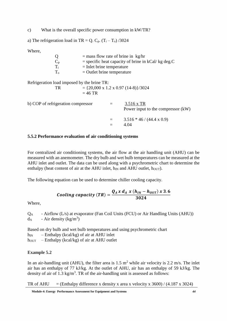
Module-4: Energy Performance Assessment for Equipment and Systems 44
c) What is the overall specific power consumption in kW/TR?
a) The refrigeration load in TR = Q. Cp. (Ti – To) /3024
Where,
Q = mass flow rate of brine in kg/hr
Cp = specific heat capacity of brine in kCal/ kg deg.C
Ti = Inlet brine temperature
To = Outlet brine temperature
Refrigeration load imposed by the brine TR:
TR = {20,000 x 1.2 x 0.97 (14-8)}/3024
= 46 TR
b) COP of refrigeration compressor = 3.516 x TR
Power input to the compressor (kW)
= 3.516 * 46 / (44.4 x 0.9)
= 4.04
5.5.2 Performance evaluation of air conditioning systems
For centralized air conditioning systems, the air flow at the air handling unit (AHU) can be
measured with an anemometer. The dry bulb and wet bulb temperatures can be measured at the
AHU inlet and outlet. The data can be used along with a psychrometric chart to determine the
enthalpy (heat content of air at the AHU inlet, hIN and AHU outlet, hOUT).
The following equation can be used to determine chiller cooling capacity.
𝑪𝒐𝒐𝒍𝒊𝒏𝒈 𝒄𝒂𝒑𝒂𝒄𝒊𝒕𝒚 (𝑻𝑹) =𝑸𝑨 𝒙 𝒅𝑨 𝒙 (𝒉𝑰𝑵 − 𝒉𝑶𝑼𝑻) 𝒙 𝟑. 𝟔
𝟑𝟎𝟐𝟒
Where,
QA - Airflow (L/s) at evaporator (Fan Coil Units (FCU) or Air Handling Units (AHU))
dA - Air density (kg/m3)
Based on dry bulb and wet bulb temperatures and using psychrometric chart
hIN – Enthalpy (kcal/kg) of air at AHU inlet
hOUT – Enthalpy (kcal/kg) of air at AHU outlet
Example 5.2
In an air-handling unit (AHU), the filter area is 1.5 m2 while air velocity is 2.2 m/s. The inlet
air has an enthalpy of 77 kJ/kg. At the outlet of AHU, air has an enthalpy of 59 kJ/kg. The
density of air of 1.3 kg/m3. TR of the air-handling unit is assessed as follows:
TR of AHU = (Enthalpy difference x density x area x velocity x 3600) / (4.187 x 3024)

Module-4: Energy Performance Assessment for Equipment and Systems 45
= (77-59) x 1.3 x 1.5 x 2.2 x 3600 / (4.187x 3024)
= 21.96 TR
Indicative TR profile (for Air conditioning)
• Small office cabins: 0.1 TR/m2
• Medium size office (10–30 people occupancy) with central A/C: 0.06 TR/m2
• Large multistoried office complexes with central A/C: 0.04 TR/m2
Heat load can also be calculated theoretically by estimating the various heat loads, both sensible
and latent, in the air – conditioned room (refer standard air conditioning hand books). The
difference between these two indicates the losses by way of leakages, unwanted loads, heat
ingress etc.
Example 5.3
The measured values of a 20 TR package air conditioning plant are as follows:
Average air velocity across suction side filter: 2.5 m/s
Cross Sectional area of suction: 1.2 m2
Inlet air
Dry Bulb temperature :20oC,
Wet Bulb temperature : 14oC,
Enthalpy : 9.37 kcal/kg
Outlet air
Dry Bulb temperature : 12.7oC,
Wet Bulb temperature : 11.3 oC;
Enthalpy : 7.45 kcal/kg
Specific volume of air : 0.85 m3/kg
Power Measurements
Compressor: 10.69 kW
Pump: 4.86 kW
Cooling tower fan: 0.87 kW
Air flow rate = 2.5 x 1.2 = 3 m3/sec = 10800 m3/hr
Cooling effect delivered = [(9.37-7.45) x10800]/ (0.85 x 3024) = 8.07 TR = 28.32 kW
Compressor kW/TR = 10.69/8.07 = 1.32
Overall kW/TR = (10.69+4.86+0.87)/8.07 = 2.04
Energy Efficiency Ratio (EER) in kW/kW = 28.32/10.69 = 2.65

Module-4: Energy Performance Assessment for Equipment and Systems 46
Example 5.4
Figure 5.1: Parameters of a centrifugal chiller
Evaluate the CoP of centrifugal chiller.
Find the ratio of evaporator refrigeration load (TR) to condenser heat rejection load (TR)
Refrigeration load (TR) : (m x Cp x T)/3024
: 80 x 3600 x 1 x (13-8)/3024
: 476 TR
Coefficient of performance (COP) : Cooling effect (kW)
Power input to compressor (kW)
: (476TRx3024/860) / 300= 5.579
Evaporator cooling load (TR) : 476 TR
Condenser heat rejection load (TR) : 185 x 3600 x (28 – 25.2)/3024
: 616 TR
Ratio : Evaporator = 476= 0.77
Condenser 616
Example 5.5
Details of centrifugal chiller and vapour absorption chiller (VAM) are given in the following
Table:
Sl.
No. Parameter
Centrifugal
Chiller VAM
1 Chilled water flow (m3/h) 192 183

Module-4: Energy Performance Assessment for Equipment and Systems 47
2 Condenser water flow (m3/h) 245 360
3 Chiller inlet water temperature (0C) 13 14.5
4 Condenser water inlet temperature (0C) 28 32
5 Chiller outlet water temperature (0C) 7.8 9.2
6 Condenser water outlet temperature (0C) 36.2 40.7
7 Chilled water pump consumption (kW) 32 31
8 Condenser water pump consumption (kW) 38 52
9 Cooling tower fan consumption (kW) 9 22
If the compressor of centrifugal chiller consumes 205 kW, the steam consumption for VAM is
1620 kg/Hr. Calculate the following:
1. Refrigeration load delivered (TR) for both systems?
2. Condenser Heat load (TR) for both systems?
3. Compare auxiliary power consumption for both systems, give reason?
Solution:
Compression Chiller vs. VAM
Sl.
No. Parameter
Centrifugal
Chiller VAM
1
Refrigeration load delivered (TR)
= Mass of Chilled water flow x Specific heat x
Delta T of Chilled water
= 192 m3/hr * 1000kg/m3 *1 kcal/kg 0C * (Sl. No.
3. – Sl. No. 5) / 3024
330.16
320.73
2
Condenser heat load delivered (TR)
= Mass of condenser water flow x Specific heat *
Delta T of condenser water
= Sl. No.2 m3/hr * 1000kg/m3*1 kcal/kg0C * (Sl.
No. 6 – Sl. No. 4) / 3024
664.35
1035.71
3 Auxiliary Power Consumption (kW) = (Sl. No. 7 +
Sl. No. 8 + Sl. No. 9) 79 105
The auxiliary power consumption in case of VAM system is higher because heat
rejection in VAM condenser is comparatively higher than centrifugal chiller with
approximate similar cooling load.
4 Total Energy Consumption:
284 kW
(Auxiliary Power of
79kW and Chiller
consumption of 205
Auxiliary
Power of 105
kW and Steam
consumption of
1620 kg/hr

Module-4: Energy Performance Assessment for Equipment and Systems 48
Example 5.6
The operating parameters of a Vapor Compression Refrigeration system are indicated below.
Parameter Chiller side Condenser side
Water Flow (m3/hr) 89 87
Inlet Temperature (oC) 10.1 32.3
Outlet Temperature (oC) 6.8 36.6
Density (kg/m3) 1000 990
Find the COP of the Refrigeration system ignoring heat losses.
Refrigeration Effect = 89 x 1000 x (10.1 – 6.8) = 293700 kcal/hr
Condenser load = 87 x 990 x (36.6 – 32.3) = 370359 kcal/hr
Compressor work = Condenser load – Refrigeration effect
= 370359 – 293700
= 76659 kCal/hr
COP. = Refrigeration Effect/ Compressor work
= 293700/76659
= 3.83
Example 5.7
A pharmaceutical unit had installed a centralized refrigeration system of 120 TR Capacity
several years ago. The refrigeration system operates 24 hours a day, 200 days per annum and
the average electricity cost is Rs. 4.5/ kWh. The following are the key operational parameters.
Compressor operating current and power factor : 153 amps. 0.9 pf
Condenser pump operating current and power factor: 43 amps, 0.88 pf
Chiller pump operating current and power factor : 25 amps, 0.9 pf
CT fan operating current and power factor : 20 amps. 0.65 pf
ΔT across the chiller (evaporator) : 3.5OC
Chilled water flow : 23 Lit / Sec
Total head developed by chiller pump : 35 mtrs.
Condenser water flow : 41 Lit / Sec
Total head developed by condenser pump : 30 mtrs.
PS: all the motors operate at 415 Volts and efficiency of 90%
Calculate:
The power consumed by the compressor, condenser pump, chiller pump and CT fan.
TR developed by the system
Specific power consumption i.e. overall kW/TR and COP and Energy Efficiency ratio
(EER)

Module-4: Energy Performance Assessment for Equipment and Systems 49
Combined efficiency (motor and pump) of condenser and chiller pumps
The unit proposes to replace the existing condenser and chilled water pumps with efficient
pumps having a combined efficiency of 65%. Also the unit goes in for condenser cleaning by
which the power consumption of compressor has reduced by 10%.
Calculate:
The envisaged power consumption of the compressor, condenser and chiller pump
Hourly energy savings (compressor, condenser and chilled water pump)
Annual energy and equivalent monetary savings (compressor, condenser and chilled
water pump)
Specific power consumption i.e. overall kW/ TR and COP and Energy Efficiency ratio
(EER)
Solution
Present Condition:
Compressor Motor Power : 99 kW
Condenser Pump Motor Power : 27.2 kW
Chiller Pump Motor Power : 16.2 kW
CT Fan : 9.4 kW
Total Power : 151.8 kW
TR Devp : (23 * 3600 * 3.5 / 3024) = 95.83
Sp. Power : 1.58 kW/ TR
Compressor kW/TR : 99/95.83
: 1.03 kW/tR
COP : 3.516/kW/TR = 3.41
EER : 12/kW/TR
: 11.65
Condenser pump efficiency : 44.4%
Chiller pump efficiency : 48.8%
Proposed condition:
Compressor Motor Power : 89 kW
Condenser Pump Motor Power : 18.6 KW
Chiller Pump Motor Power : 12.2 kW
CT Fan : 9.4 kW
Total Power : 129.2 kW
TR Devp : 95.83 TR i.e. (23 LPS * 3600 Sec * 3.5 / 3024)
Sp. Power : 1.35 kW/ TR
Compressor kW/TR : 89/95.83 = 0.93 kW/TR
COP : 3.516 / 0.93 = 3.78
EER : 12 / 0.93 = 12.90

Module-4: Energy Performance Assessment for Equipment and Systems 50
Compressor Condenser
Pump
Chiller
Pump
Hourly energy savings – kWh (99-89) = 10 (27.2-18.6) =
8.6
(16.2–12.2)
= 4.0
Annual energy savings – kWh (4800 hrs) 48000 41280 19200
5.5.3 Procedure for Performance Evaluation of Vapour Absorption Refrigeration
(VAR) System
It should be ensured that the evaporator, condenser and generator are nearly at same operating
conditions throughout the duration of the test. The vapour absorption system auxiliaries include
chiller water pumps, condenser water pumps, cooling tower fans and performance assessment
of these auxiliaries can be carried out in the same manner as applicable to vapour compression
refrigeration system auxiliaries.
5.5.4 Estimation of performance at evaporator side
The performance evaluation involves the measurement of following parameters.
Refrigeration effect (QC)
Chilled water flow rate in the evaporator.
Chilled water temperatures at the evaporator inlet and outlet.
Thermal power input (Qin)
Steam mass flow rate in case of steam heated vapour absorption chilling package.
Fuel flow rate in case of direct fuel fired vapour absorption package.
Measuring instruments:
The measuring instruments should be duly calibrated.
Direct reading thermometers can be used for measuring temperature. The least count
for temperature indicating instruments should be 0. 1°C.
The method mentioned in VCR system can be used for water flow rate measurement.
For steam heated vapour absorption chilling package, the thermal power consumption
may be measured with any of the following instruments:
a) Calibrated in-line steam flow meter.
b) Collection of condensate in calibrated volume (container) for a defined time period.
The time period should be measured with a digital chronometer (stop-watch) with
least count of 1/100 second. The condensate may be cooled to reduce the flash steam
losses.
For fuel fired vapour absorption systems, the thermal power may be measured with any
of the following instruments:

Module-4: Energy Performance Assessment for Equipment and Systems 51
a) Calibrated In—line fuel flow meter.
b) Fuel level difference (for liquid fiiels) for a defined time period in a calibrated day
tank. The time period should be measured with a digital chronometer (stop-watch)
with least count of l/100 second.
Performance calculations:
Coefficient of performance, COP at evaporator side
For Steam heated Vapour Absorption Chilling Packages,
For Direct Fuel-Fired Vapour Absorption Chilling Packages,
Where,
Qin
= Thermal energy input in kW
Qe = Refrigeration effect in kW
Me = Chilled water flow rate in the evaporator, kg/h
Cp = Specific heat ofwater, kJ/kg-K
tin = Chilled water temperature at evaporator inlet, K
tout = Chilled water temperature at evaporator outlet, K
Mst = Steam consumption rate, kg/hr
hst = Enthalpy of steam at operating pressure, kJ/kg
hcond = Enthalpy of condensate, kJ/kg
Mf = Fuel consumption rate, kg/hr
GCV = Gross calorific value of fuel, kJ/kg
5.5.5 Estimation of performance at condenser side (water cooled condenser)
The performance evaluation involves the measurement of following parameters.
Heat rejected at the condenser (QC)
Cooling water flow rate in the condenser.
Cooling water temperatures at absorber inlet and the condenser outlet.

Module-4: Energy Performance Assessment for Equipment and Systems 52
Thermal energy input (Qin)
Steam mass flow rate in case of steam heated vapor absorption chilling package.
Fuel flow rate in case of direct fuel fired vapor absorption package.
Determination of refrigeration effect and COP:
i. The refrigeration effect and COP can be determined from the overall heat balance of the
condenser and VAR system.
ii. Heat rejected at the condenser (Q) is equal to refrigeration effect heat (QC) plus thermal
energy input (absorbed) by the system (Qin)
Performance calculations:
a) COP at condenser side for steam heated vapour absorption package
Figure 5.2
At condenser,
Refrigeration effect heat = Heat rejected in the condenser — Thermal energy input
Qe = Qc — Qin
Therefore,

Module-4: Energy Performance Assessment for Equipment and Systems 53
b) COP at condenser side for direct fuel fired vapour absorption packages
Figure 5.3
At condenser,
Refrigeration effect heat = Heat rejected in the condenser — Heat input
Therefore,
Where,
Mc = Cooling water flow rate in the condenser, kg/h
twi = Cooling water temperature at absorber inlet, K for VAR chiller
tWo = Cooling water temperature at condenser outlet, K
ηcomb= Combustion efficiency
Combustion Efficiency Calculations:
The method described below can be used for estimating combustion efficiency of a direct fuel
fired absorption chilling unit. The methodology is the “Indirect Method” to estimate
combustion efficiency (ηcomb), wherein the losses are estimated from flue gas analysis to
estimate efficiency.

Module-4: Energy Performance Assessment for Equipment and Systems 54
Observations:
Flue gas analysis:
a) Average % O2 (V/V)
b) Flue / stack gas temperature, Tf (°C)
c) Average ambient air temperature, Ta (°C)
Fuel analysis:
a) % Moisture (W/W), M
b) % Carbon (W/W), C
c) % Hydrogen (W/W), H2
d) % Oxygen (w/W), O2
e) % Nitrogen (w/w), N2
f) % Sulphur (W/W), S
g) Gross calorific valve, GCV (kcal/kg)
Calculations:
Theoretical air
required for
combustion
= [(11.6 x C) + {34.8 x (H2-O2 /8)}+(4.35 x S)]/100 kg/kg of
fuel. [from fuel analysis]
Where C, H2, O2 and S are the percentage of carbon, hydrogen,
oxygen and sulphur present in the fuel.
% Excess air
supplied
=
[from fuel analysis]
Actual mass of air
supplied
= {1 + EA/ 100} X Theoretical air
% Dry gas loss (D.G.L.):
D.G.L. =
Where,
mf = Mass of dry flue gas in kg/kg of fuel
Total mass of dry flue gas /kg of fuel = Actual mass of air supplied/kg of fuel +1 kg of fuel
— (9H2 + M)
Cpf = Specific heat of flue gas in kcal/kg
e) % Wet gas loss (W.G.L.): =
Where, 584 = Latent heat corresponding to partial pressure of water vapor
0.45 = Specific heat of water vapor / superheated steam in kcal/kg°C

Module-4: Energy Performance Assessment for Equipment and Systems 55
f) Total stack loss or flue gas loss (%) = D.G.L. + W.G.L.
g) Combustion efficiency by indirect method, ncomb = (100 - % Total flue gas losses) = Heat
absorbed by the generator of VAR system.
Note: In this method only the major combustion losses namely, dry and wet flue gas losses are
considered. All other losses are considered insignificant and hence ignored.
5.5.6 Performance assessment of Vapor Absorption Refrigeration (VAR) system:
Example 5.8
This is a sample calculation for a Vapor Absorption Chilling Package. Measurements are
shown along with equations and estimation of results.
Equipment Specification for VAR system
Parameter Unit Quantity
Rated Generator temperature (in case of VAR chilling package) 165
Rated Capacity at Full Load TR 1180
Fluid being cooled in the evaporator Water
Rated Evaporator Fluid Flow Rate, Me m3/h 713
Rated Evaporator inlet temperature, tin ◦C 12
Rated Evaporator outlet temperature, tout ◦C 7
Rated Condenser Water Flow Rate, Mc m3/h 1427
Rated Condenser inlet temperature, twi ◦C 27
Rated Condenser outlet temperature, tWO ◦C 32
Method 1: Evaporator side
Estimation of performance from refrigeration effect in evaporator for steam heated vapor
chilling packages (Chilling water)
Parameter Unit Value
Ambient dry bulb temperature ⁰C 38
Ambient wet bulb temperature ⁰C 25
Chilled water flow, Me m 3/h 620
Chilled water density, p kg/ m3 1000
Specific heat of chilled water, CD kJ/kg/K 4_18
Chilled water temperature at evaporator inlet, tin ⁰C 88
Chilled water temperature at evaporator outlet,
tout ⁰C 6.8
Cooling Water flow, Mc m3/h 954
Cooling water inlet temperature, twi ⁰C 26.6
Cooling water outlet temperature, tWO ⁰C 299
Refrigeration Effect, Qe
kJ/h 5 1 83200

Module-4: Energy Performance Assessment for Equipment and Systems 56
Refrigeration Effect, R Qe / (3.516 x 3600)
TR 410
Generator temperature ⁰C 120
Steam Pressure kPa 300
Enthalpy of steam, hst kJ/kg 2734
Steam consumption rate, Mst kg/h 3443
Condensate temperature ⁰C 100
Enthalpy of condensate, hcond kJ/kg 418
Estimated Thermal energy Input, Qin kJ/h
kJ/h 7974332
Coefficient of Performance, COP kW/kW QP/ Qin
0.65
Specific Energy consumption, SEC kJ/TR
kJ/TR 3443 X (2734 — 418) / 410
kJ/TR 19449
kcal/TR 4645
Method 2: Condenser side
Estimation of performance from heat rejection in Water Cooled Condenser for steam heated
vapor absorption chilling packages (Cooling water)
Inference: The performance parameters estimated above show a deviation from the actual
design values. This may due to operation of the chiller at less than 50% load.

Module-4: Energy Performance Assessment for Equipment and Systems 57
Fig
ure
5.4
: P
sych
rom
etri
c ch
art

Module-4: Energy Performance Assessment for Equipment and Systems 58
Example 5.9
In an air conditioning system of a food processing industry, the cold air flow rate is 20,000
m3/hr at a density of 1.2 kg/m3 .The inlet and outlet enthalpy of the air are 105 kJ/kg and 80
kJ/kg. The COP of the existing vapor compression system is 3.75. The efficiency of the motor
coupled with the compressor is 90%.
The management wants to install a Vapor Absorption System (VAR).The saturated steam for
VAR will be supplied either from a new waste heat boiler to be installed with the existing DG
sets or from the existing FO fuel fired boiler. The plant is operating for 8000 hr/annum. The
investment of VAR system is Rs. 20 lakhs. The investment for waste heat boiler is Rs. 6 lakhs.
The power cost is Rs. 6/kWh.
As an energy auditor which one of the following options will you recommend to the
management?
Option-1: Supply steam from the existing FO fuel fired boiler to VAR system and avoid the
investment of waste heat boiler
Option-2: Supply steam from the waste heat boiler, which needs an investment in addition to
VAR system
The steam consumption per TR will be 5.5 kg/TR. The cost ofF0 is Rs.32,000/ ton. The
evaporation ratio of the existing FO fired boiler is 14. Neglect losses in transmission of steam
and chilled water.
Solution:
Existing Base Case VCR System
TR Rating
= 47.38 TR
COP = 3.75
COP
Compressor power input
= 44.43 kW
Motor input power = 44.43/0.9 = 49.37 kW
Annual Energy Consumption = 49.37 x 8000 = 3.95 Lakhs kWh
Annual cost in VCR system (Base Case) =3.95 X 6 = Rs. 23.7 Lakhs
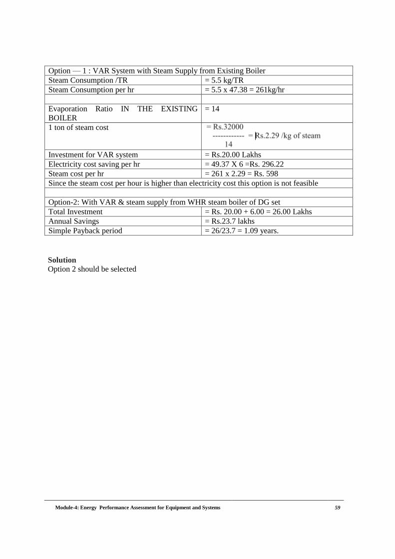
Module-4: Energy Performance Assessment for Equipment and Systems 59
Option — 1 : VAR System with Steam Supply from Existing Boiler
Steam Consumption /TR = 5.5 kg/TR
Steam Consumption per hr = 5.5 x 47.38 = 261kg/hr
Evaporation Ratio IN THE EXISTING
BOILER
= 14
1 ton of steam cost
Investment for VAR system = Rs.20.00 Lakhs
Electricity cost saving per hr = 49.37 X 6 =Rs. 296.22
Steam cost per hr = 261 x 2.29 = Rs. 598
Since the steam cost per hour is higher than electricity cost this option is not feasible
Option-2: With VAR & steam supply from WHR steam boiler of DG set
Total Investment = Rs. 20.00 + 6.00 = 26.00 Lakhs
Annual Savings = Rs.23.7 lakhs
Simple Payback period = 26/23.7 = 1.09 years.
Solution
Option 2 should be selected

Module-4: Energy Performance Assessment for Equipment and Systems 60
Chapter 6: Boiler Performance Assessment
6.1 Introduction
The key performance parameters of boilers such as efficiency and evaporation ratio, reduces
with time, due to poor combustion, heat transfer fouling and poor operation and maintenance.
Deterioration of fuel quality and water quality also leads to poor performance of boiler.
Periodic efficiency testing of boiler helps us to find out how far the boiler efficiency drifts
away from the best efficiency. Any observed abnormal deviations could be investigated to
identify problem areas for necessary corrective action. Assessing the current level of efficiency
and performance of boiler is the first step for energy conservation activity.
6.2 Purpose of the Performance Test
To find out the efficiency of the boiler
To find out the Evaporation Ratio
The purpose of the performance test is to determine actual performance and efficiency of the
boiler and compare it with design values or norms. The performance parameters can be used
for tracking variations and initiating corrective actions.
The procedures for boiler efficiency testing for both oil-fired and gas-fired fired boilers are
outlined.
6.3 Performance Terms and Definitions
6.3.1 Direct method of testing
This is also known as 'input-output method' due to the fact that it needs only the useful output
(steam) and the heat input (i.e. fuel) for evaluating the efficiency. This efficiency can be
evaluated using the formula:
𝐵oiler Efficiency, =Heat output
Heat input X 100
𝑩𝒐𝒊𝒍𝒆𝒓 𝑬𝒇𝒇𝒊𝒄𝒊𝒆𝒏𝒄𝒚, =𝑯𝒆𝒂𝒕 𝒊𝒏 𝒔𝒕𝒆𝒂𝒎 𝒐𝒖𝒕𝒑𝒖𝒕 (𝒌𝑪𝒂𝒍)
𝑯𝒆𝒂𝒕 𝒊𝒏 𝒇𝒖𝒆𝒍 𝒊𝒏𝒑𝒖𝒕 (𝒌𝑪𝒂𝒍) 𝑿 𝟏𝟎𝟎

Module-4: Energy Performance Assessment for Equipment and Systems 61
Evaporation ratio =Quantity of steam generation
Quantity of fuel consumption
Figure 6.1
𝑩𝒐𝒊𝒍𝒆𝒓 𝒆𝒇𝒇𝒊𝒄𝒊𝒆𝒏𝒄𝒚
=𝑭𝒍𝒐𝒘 𝒓𝒂𝒕𝒆 𝒐𝒇 𝒔𝒕𝒆𝒂𝒎 𝒙 (𝑺𝒕𝒆𝒂𝒎 𝒆𝒏𝒕𝒉𝒂𝒍𝒑𝒚 − 𝑭𝒆𝒆𝒅 𝒘𝒂𝒕𝒆𝒓 𝒆𝒏𝒕𝒉𝒂𝒍𝒑𝒚
𝑭𝒖𝒆𝒍 𝒇𝒊𝒓𝒊𝒏𝒈 𝒓𝒂𝒕𝒆 𝒙 𝑪𝒂𝒍𝒐𝒓𝒊𝒇𝒊𝒄 𝒗𝒂𝒍𝒖𝒆 𝑿 𝟏𝟎𝟎
6.3.2 Measurements Required for Direct Method Testing
Heat input
Both heat input and heat output must be measured. The measurement of heat input requires
knowledge of the calorific value of the fuel and its flow rate in terms of mass or volume,
according to the type of the fuel.
For gaseous fuel: A gas meter of the approved type can be used and the measured volume
should be corrected for temperature and pressure. A sample of gas can be collected for calorific
value determination, but it is acceptable to use declared calorific value of gas suppliers.
For liquid fuel: Heavy fuel oil is very viscous, and this property varies sharply with
temperature. The meter, which is usually installed on the combustion appliance, should be
regarded as a rough indicator only and, for test purposes, a meter calibrated for the particular
oil is to be used. The best is the use of an accurately calibrated day tank.
Heat output
There are several methods, which can be used for measuring heat output. With steam boilers,
an installed steam meter can be used to measure flow rate, but this must be corrected for
temperature and pressure. Modern flow meters of the variable-orifice or vortex shedding types
are recommended.
The alternative to measuring steam in small boilers is to measure feed water entering the boiler.

Module-4: Energy Performance Assessment for Equipment and Systems 62
This can be done by previously calibrating the feed tank and noting down the levels of water
at the beginning and end of the trial. Care should be taken not to pump water during this period.
Heat addition for conversion of feed water (at inlet temperature) to steam, is considered for
heat output.
Intermittent blow down, if deployed in the boiler, should be avoided during the trial period. In
case of boilers with continuous blow down, the heat loss due to blow down should be calculated
and added to the heat in steam.
6.3.3 Boiler Efficiency by Direct Method: Calculation and Example
Test Data and Calculation
Water consumption and coal consumption are to be measured in a coal-fired boiler at hourly
intervals. Weighed quantities of coal are fed to the boiler during the trial period. Simultaneously
water level difference was noted to calculate steam generation during the trial period. Blow
down was avoided during the test. The measured data and calculations are as follows:
Direct Method (sample calculations)
Type of boiler: Coal-fired boiler
Table 6.1
Heat input data
Quantity of coal fired: 1.6
TPH
GCV of coal: 4000 kCal/kg
Heat output data
Quantity of steam generated: 8 TPH
Steam pressure/ temperature: 10 kg/cm2 (g)/180oC
Enthalpy of steam (dry and saturated) : 665 kCal/kg
Feed water temperature: 85oC
Enthalpy of feed water: 85 kCal/kg
Boiler efficiency () = Q x (H-h) x 100
(q x GCV)
Where,
Q = Quantity of steam generated per hour (kg/hr)
Q = Quantity of fuel used per hour (kg/hr)
GCV = Gross calorific value of fuel (kCal/kg)
H = Enthalpy of steam (kCal/kg)
H = Enthalpy of feed water (kCal/kg)
Boiler efficiency () = 8 TPH x 1000 kg/T x (665-85) x 100
1.6 TPH x 1000 kg/T x 4000 kCal/kg
= 72.5 %
Evaporation Ratio = 8 tonne of steam/1.6 tonne of coal
= 5
Merits and Demerits of Direct Method
Merits
Plant people can quickly evaluate the efficiency of boilers
Only few parameters required for computation
Only few instruments for monitoring

Module-4: Energy Performance Assessment for Equipment and Systems 63
Demerits
Does not give indicate why efficiency of boiler is lower
Does not account various losses
High (erroneous) Evaporation ratio and efficiency of steam is wet due to water
carryover
Determination of Evaporation ratio
The simplest way to calculate fuel-to-steam efficiency is using steam generation and fuel
consumption data from operating log book. Steam-Fuel consumption ratio, which is commonly
called Evaporation Ratio, is given by the relation:
Evaporation Ratio = Feed water consumption (kg/hr)
Fuel consumption (kg/hr)
The two metering devices, fuel consumption meter and feed water flow meter, are needed for
determining Evaporation Ratio. These two values should be recorded in the log sheet. For
calculating steam rate, blow down rate is deducted. Typical Evaporation ratios of boilers for
various fuels are as follows:
Table 6.2: Typical Evaporation Ratio
Type of fuel Typical Evaporation Ratio
Fuel oil
Solid fuel
Gaseous fuel
~ 13–14 kg steam/kg fuel oil
~ 4–5 kg steam/kg solid fuel
~ 13 kg steam/Nm3 gaseous fuel
If the Evaporation Ratio is lower than the typical value, it means boiler efficiency is
deteriorating. Evaporation Ratio after commissioning or annual boiler overhaul can be
considered as the benchmark value. For every one unit reduction in Evaporation Ratio, the
boiler efficiency reduces by 1%.
6.3.4 The Indirect Method Testing
Description
All the losses occurring in the boiler are measured. The efficiency can then be arrived at, by
subtracting the heat loss fractions from100. An important advantage of this method is that the
errors in measurement do not make significant change in efficiency.
Most performance tests in industrial boilers are carried out using indirect method. The reference
standards for Boiler Testing at a site for the indirect method are the British Standard, BS
845:1987 and the USA Standard ASME PTC-4-1 Power Test Code Steam Generating Units.

Module-4: Energy Performance Assessment for Equipment and Systems 64
Figure 6.2
The following losses are applicable to liquid, gas and solid fired boiler
L1 Loss due to dry flue gas (sensible heat)
L2 Loss due to hydrogen in fuel (H2)
L3 Loss due to moisture in fuel (H2O)
L4 Loss due to moisture in air (H2O)
L5 Loss due to carbon monoxide (CO)
L6 Loss due to surface radiation, convection and other unaccounted losses*
*Losses which are insignificant and are difficult to measure.
The following losses are applicable to solid fuel fired boiler in addition to above.
L7 - Unburnt losses in fly ash (carbon)
L8 - Unburnt losses in bottom ash (carbon)
Boiler Efficiency by indirect method = 100 (L1 + L2 + L3 + L4 + L5 + L6 + L7 + L8)
Measurements Required for Performance Assessment Testing
The following parameters need to be measured, as applicable for the computation of boiler
efficiency and performance:
a) Flue gas analysis
Percentage of CO2 or O2 in flue gas
Percentage of CO in flue gas
Temperature of flue gas
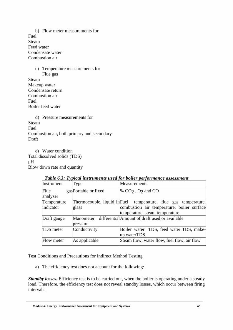
Module-4: Energy Performance Assessment for Equipment and Systems 65
b) Flow meter measurements for
Fuel
Steam
Feed water
Condensate water
Combustion air
c) Temperature measurements for
Flue gas
Steam
Makeup water
Condensate return
Combustion air
Fuel
Boiler feed water
d) Pressure measurements for
Steam
Fuel
Combustion air, both primary and secondary
Draft
e) Water condition
Total dissolved solids (TDS)
pH
Blow down rate and quantity
Table 6.3: Typical instruments used for boiler performance assessment
Instrument Type Measurements
Flue gas
analyzer
Portable or fixed % CO2 , O2 and CO
Temperature
indicator
Thermocouple, liquid in
glass
Fuel temperature, flue gas temperature,
combustion air temperature, boiler surface
temperature, steam temperature
Draft gauge Manometer, differential
pressure
Amount of draft used or available
TDS meter Conductivity Boiler water TDS, feed water TDS, make-
up waterTDS.
Flow meter As applicable Steam flow, water flow, fuel flow, air flow
Test Conditions and Precautions for Indirect Method Testing
a) The efficiency test does not account for the following:
Standby losses. Efficiency test is to be carried out, when the boiler is operating under a steady
load. Therefore, the efficiency test does not reveal standby losses, which occur between firing
intervals.

Module-4: Energy Performance Assessment for Equipment and Systems 66
Blow down loss. The amount of energy wasted by blow down varies over a wide range.
Soot blower steam. The amount of steam used by soot blowers is variable and depends on the
type of fuel.
Auxiliary equipment energy consumption. The efficiency test does not account for the energy
usage by auxiliary equipment, such as burners, fans, and pumps.
b) Preparations and pre conditions for testing:
Burn the specified fuel at the required rate.
Conduct the tests while the boiler under steady load conditions. Avoid testing during
warming up of boilers from a cold condition
Obtain the relevant charts /tables (e.g. Steam chart) for the additional data.
Determine general method of operation, sampling and analysis of fuel and ash.
Ensure accuracy of fuel and ash analysis in the laboratory.
Check the type of blow down and method of measurement
Ensure proper operation of all instruments.
Inspect for any air infiltration in the combustion zone.
c) Flue gas sampling location
Flue gas sampling point for temperature and gas analysis is ideally carried out at zone of
maximum gas flow which normally coincides with zone of maximum temperature.
d) Options of flue gas analysis
Check the Oxygen Test with the Carbon Dioxide Test
If continuous-reading oxygen meter or equipment is installed in boiler plant, use oxygen
reading. Occasionally use portable test equipment that checks for both oxygen and carbon
dioxide.
If the carbon dioxide test does not give the same results as the oxygen test, something is wrong.
One (or both) of the tests could be wrong, perhaps because of stale chemicals or drifting
instrument calibration. Another possible reason could be that outside air is being picked up
along with the flue gas. This occurs if the combustion gas area operates under negative pressure
and there are leakages in the boiler casing.
Carbon Monoxide Test
The carbon monoxide content of flue gas is a good indicator of incomplete combustion with
all types of fuels, as long as they contain carbon. Normally, carbon monoxide in the flue gas is
minimal with ordinary amounts of excess air in the flue gas, but sharply rises as soon as fuel
combustion starts to become incomplete.
e) Planning for the testing:
The testing is to be conducted for duration of 4 to 8 hours in a normal production day.
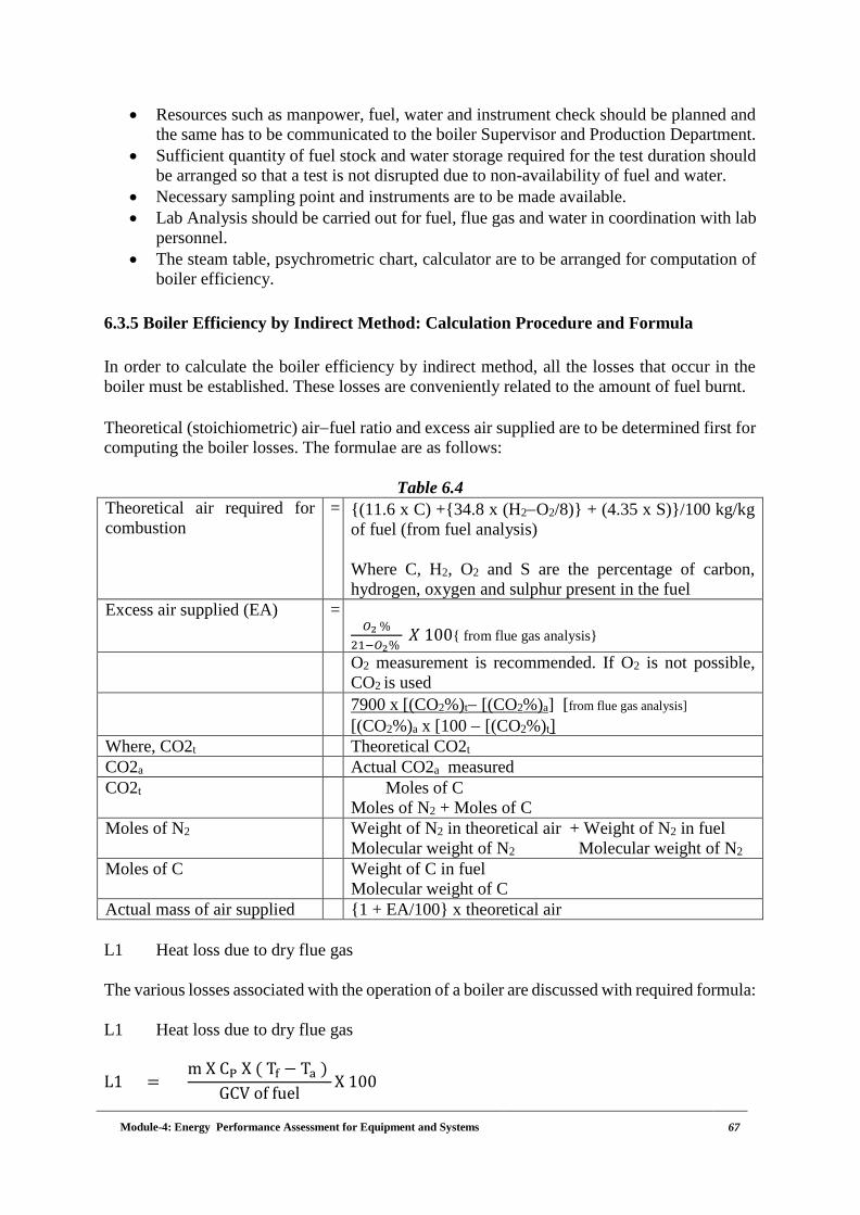
Module-4: Energy Performance Assessment for Equipment and Systems 67
Resources such as manpower, fuel, water and instrument check should be planned and
the same has to be communicated to the boiler Supervisor and Production Department.
Sufficient quantity of fuel stock and water storage required for the test duration should
be arranged so that a test is not disrupted due to non-availability of fuel and water.
Necessary sampling point and instruments are to be made available.
Lab Analysis should be carried out for fuel, flue gas and water in coordination with lab
personnel.
The steam table, psychrometric chart, calculator are to be arranged for computation of
boiler efficiency.
6.3.5 Boiler Efficiency by Indirect Method: Calculation Procedure and Formula
In order to calculate the boiler efficiency by indirect method, all the losses that occur in the
boiler must be established. These losses are conveniently related to the amount of fuel burnt.
Theoretical (stoichiometric) airfuel ratio and excess air supplied are to be determined first for
computing the boiler losses. The formulae are as follows:
Table 6.4
Theoretical air required for
combustion
= {(11.6 x C) +{34.8 x (H2O2/8)} + (4.35 x S)}/100 kg/kg
of fuel (from fuel analysis)
Where C, H2, O2 and S are the percentage of carbon,
hydrogen, oxygen and sulphur present in the fuel
Excess air supplied (EA) = 𝑂2 %
21−𝑂2% 𝑋 100{ from flue gas analysis}
O2 measurement is recommended. If O2 is not possible,
CO2 is used
7900 x [(CO2%)t [(CO2%)a] [from flue gas analysis]
[(CO2%)a x [100 [(CO2%)t]
Where, CO2t Theoretical CO2t
CO2a Actual CO2a measured
CO2t Moles of C
Moles of N2 + Moles of C
Moles of N2 Weight of N2 in theoretical air + Weight of N2 in fuel
Molecular weight of N2 Molecular weight of N2
Moles of C Weight of C in fuel
Molecular weight of C
Actual mass of air supplied {1 + EA/100} x theoretical air
L1 Heat loss due to dry flue gas
The various losses associated with the operation of a boiler are discussed with required formula:
L1 Heat loss due to dry flue gas
L1 = m X CP X ( Tf − Ta )
GCV of fuelX 100

Module-4: Energy Performance Assessment for Equipment and Systems 68
L1 = % heat loss due to dry flue gas
m = Mass of dry flue gas in kg/kg of fuel
= Combustion products from fuel: CO2 +SO2 +Nitrogen in fuel+ Nitrogen in the
Actual mass of air supplied + O2 in flue gas
(H2O/water vapour in the flue gas should not be considered on dry basis)
Cp = Specific heat of flue gas kCal/kgoC
Tf = Flue gas temperature in oC
Ta = Ambient temperature in oC
Note 1: For Quick and simple calculation of boiler efficiency use the following.
A: Simple method can be used for determining the dry flue gas loss as follows:
𝑷𝒆𝒓𝒄𝒆𝒏𝒕𝒂𝒈𝒆 𝒐𝒇 𝒉𝒆𝒂𝒕 𝒍𝒐𝒔𝒔 𝒅𝒖𝒆 𝒕𝒐 𝒇𝒍𝒖𝒆 𝒈𝒂𝒔 =𝒎 𝑿 𝑪𝑷 𝑿 ( 𝑻𝒇 − 𝑻𝒂 )
𝑮𝑪𝑽 𝒐𝒇 𝒇𝒖𝒆𝒍𝑿 𝟏𝟎𝟎
Total mass of flue gas (m)/kg of fuel = mass of actual air supplied/kg of fuel + 1 kg of fuel
Note 2: Water vapour is produced from hydrogen in fuel, moisture present in fuel and
atmospheric air during the combustion. The losses due to these components have not been
included in the dry flue gas loss since each loss is separately calculated as part of wet flue gas
loss.
L2 Heat loss due to evaporation of water formed due to H2 in fuel(%)
The combustion of hydrogen causes a heat loss be cause the product of combustion is water
and this water is converted to steam carrying away heat in the form of its latent heat.
L2 = 9 x H2 x {584 + Cp(Tf − Ta)}
GCV of fuelx 100
Where,
H2 = kg of hydrogen present in fuel on 1 kg basis
Cp = Specific heat of superheated steam in kCal/kg oC
Tf = Flue gas temperature in oC
Ta = Ambient temperature in oC
584 = Latent heat corresponding to partial pressure of water vapour
L3 Heat loss due to moisture present infuel
Moisture entering the boiler with the fuel leaves as a superheated vapour. This moisture loss is
made up of the sensible heat to bring the moisture to boiling point, the latent heat of evaporation
of the moisture, and the superheat required to bring this evaporated moisture (steam) to the
temperature of the exhaust gas. This loss can be calculated with the following formula:
L3 = M x {584 + Cp(Tf − Ta)}
GCV of fuelx 100
Where,
M = kg moisture in fuel on 1 kg basis

Module-4: Energy Performance Assessment for Equipment and Systems 69
Cp = Specific heat of superheated steam in kCal/kg oC
Tf = Flue gas temperature in oC
Ta = Ambient temperature in oC
584 = Latent heat corresponding to partial pressure of water vapour
L4 Heat loss due to moisture present in air
Vapour in the form of humidity in the incoming combustion air is superheated as it passes
through the boiler. Since this heat passes up the stack, it must be included as a boiler loss.
To relate this loss, the moisture content of the combustion air and the amount of air supplied
per unit mass of fuel burned must be known. The mass of vapour that air contains can be
obtained from psychrometric charts and typical values are as follows:
Table 6.5
Dry-Bulb
Temperature
Wet Bulb
Temperature
Relative Humidity Kilogram waterper
Kilogram dry air
(Humidity Factor) °C °C (%)
20 20 10 0.016
20 14 50 0.008
30 22 50 0.014
40 30 50 0.024
L4 =AAS x Humidity factor x Cp x (Tf − Ta) x 100
GCV of fuel
Where,
AAS = Actual mass of air supplied
Humidity factor = kg of water per kg of dry air
Cp = Specific heat of superheated steam in kCal/kg oC
Tf = Flue gas temperature in oC
Ta = Ambient temperature in oC
L5 Heat loss due to incomplete combustion (CO):
Products formed by incomplete combustion could be mixed with oxygen and burned again with
a further release of energy. Such products include CO, H2, and various hydrocarbons and are
generally found in the flue gas of the boilers. Carbon monoxide is the only gas whose
concentration can be determined conveniently in a boiler plant test.
L5 =%CO x C
% CO + %CO2 x
5654
GCV of fuel x 100
Where,
L5 = % heat loss due to partial conversion of C to CO
(1% = 10000 PPM)
CO = Volume of CO in flue gas leaving economizer (%)
CO2 = Actual volume of CO2 in flue gas (%)

Module-4: Energy Performance Assessment for Equipment and Systems 70
C = Carbon content kg/kg of fuel
*5654 kCal/kg - Heat loss due to partial combustion of carbon
L6 Heat loss due to radiation and convection:
The other heat losses from a boiler consist of the loss of heat by radiation and convection from
the boiler casing into the surrounding boiler house.
Normally surface loss and other unaccounted losses is assumed based on the type and size of
the boiler as given below
For industrial fire tube / packaged boiler = 1.5 to 2.5%
For industrial water tube boiler = 2 to 3%
For power station boiler = 0.4 to 1%
It can be calculated if the surface area of boiler and its surface temperature are measured and
using the following formula:
L6 = 0.548 x [ (Ts
55.55)
4
− (Ta
55.55)
4
]
+ 1.957 x (Ts − Ta)1.25 x sq. rt. of [(196.85 Vm + 68.9)
68.9]
Where,
L6 = Radiation loss in W/m2
Vm = Wind velocity in m/s
Ts = Surface temperature (K)
Ta = Ambient temperature (K)
Heat loss due to unburned carbon in fly ash and bottom ash:
Small amounts of carbon will be left in the as hand this constitutes a loss of potential heat in
the fuel. To assess these heat losses, samples of ash must be analyzed for carbon content. The
quantity of ash produced per unit of fuel must also be known.
L7 Heat loss due to unburnt in fly ash (%)
= 𝑇𝑜𝑡𝑎𝑙 𝑎𝑠ℎ 𝑐𝑜𝑙𝑙𝑒𝑐𝑡𝑒𝑑/𝑘𝑔 𝑜𝑓 𝑓𝑢𝑒𝑙 𝑏𝑢𝑟𝑛𝑡 × 𝐺. 𝐶. 𝑉 𝑜𝑓 𝑓𝑙𝑦 𝑎𝑠ℎ ×100 GCV of fuel
L8 Heat loss due to unburnt in bottom ash (%)
=𝑇𝑜𝑡𝑎𝑙 𝑎𝑠ℎ 𝑐𝑜𝑙𝑙𝑒𝑐𝑡𝑒𝑑 /𝑘𝑔𝑜𝑓𝑓𝑢𝑒𝑙𝑏𝑢𝑟𝑛𝑡 × 𝐺.𝐶.𝑉𝑜𝑓𝑏𝑜𝑡𝑡𝑜𝑚𝑎𝑠ℎ×100 GCV of fuel
Heat Balance:
Having established the magnitude of all the losses mentioned above, a simple heat balance
would give the efficiency of the boiler. The efficiency is the difference between the energy

Module-4: Energy Performance Assessment for Equipment and Systems 71
input to the boiler and the heat losses calculated.
Boiler Heat Balance:
Input/output parameter kCal / kg of fuel %
Heat Input in fuel = 100
Various Heat losses in boiler
1. Dry flue gas loss =
2. Loss due to hydrogen in fuel =
3. Loss due to moisture in fuel =
4. Loss due to moisture in air =
5. Partial combustion of C to CO =
6. Surface heat losses =
7. Loss due to Unburnt in fly ash =
8. Loss due to Unburnt in bottom ash =
Total Losses =
Boiler efficiency = 100 - (1+2+3+4+5+6+7+8)
6.4 Efficiency for an oil fired boiler (Sample calculations)
Example 6.1
The following are the data collected for a boiler using furnace oil as the fuel. Find out the boiler
efficiency by indirect method.
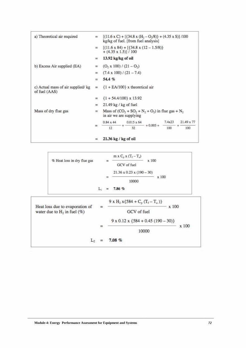
Module-4: Energy Performance Assessment for Equipment and Systems 72

Module-4: Energy Performance Assessment for Equipment and Systems 73
Summary of Heat Balance for the Boiler Using Furnace Oil
Input/Output Parameter kCal / kg of furnace
oil
%Loss

Module-4: Energy Performance Assessment for Equipment and Systems 74
Heat Input = 10000 100
Losses in boiler :
1. Dry flue gas, L1 = 786 7.86
2. Loss due to hydrogen in fuel, L2 = 708 7.08
3. Loss due to Moisture in fuel, L3 = 3.3 0.033
4. Loss due to Moisture in air, L4 = 38 0.38
5. Partial combustion of C to CO, L5 = 0 0
6. Surface heat losses, L6 = 38 0.38
Boiler Efficiency = 100 - (L1 + L2 + L3 + L4 + L6) = 84.27 %
Note: For quick and simple calculation of boiler efficiency use the following.
Simple method can be used for determining the dry flue gas loss as follows:
𝑷𝒆𝒓𝒄𝒆𝒏𝒕𝒂𝒈𝒆 𝒐𝒇 𝒉𝒆𝒂𝒕 𝒍𝒐𝒔𝒔 𝒅𝒖𝒆 𝒕𝒐 𝒇𝒍𝒖𝒆 𝒈𝒂𝒔 =𝒎 𝑿 𝑪𝑷 𝑿 ( 𝑻𝒇 − 𝑻𝒂 )
𝑮𝑪𝑽 𝒐𝒇 𝒇𝒖𝒆𝒍𝑿 𝟏𝟎𝟎
Total mass of flue gas (m)/kg of fuel =
Mass of actual air supplied/kg of fuel + 1 kg of fuel– (9 H2 + M) = 21.49 + 1 – 1.085=21.405
Dry flue gas loss in %= 21.405 x 0.23 x (190 – 30) x 100 /10000 = 7.86 %
Example 6.2 Efficiency for a cool fired boiler
The following are the data collected for a boiler using coal as the fuel. Find out the boiler
efficiency by indirect method.

Module-4: Energy Performance Assessment for Equipment and Systems 75

Module-4: Energy Performance Assessment for Equipment and Systems 76

Module-4: Energy Performance Assessment for Equipment and Systems 77

Module-4: Energy Performance Assessment for Equipment and Systems 78
Summary of Heat Balance for Coal Fired Boiler
6.5 Factors Affecting Boiler Performance
The various factors affecting the boiler performance are as follows:
Periodical cleaning of boilers
Periodical soot blowing
Proper water treatment programme and blow down control
Draft control
Excess air control

Module-4: Energy Performance Assessment for Equipment and Systems 79
Percentage loading of boiler
Steam generation pressure and temperature
Boiler insulation
Quality of fuel
All these factors individually/combined, contribute to the performance of the boiler and
reflected either in boiler efficiency or evaporation ratio. Based on the results obtained from the
testing, further improvements have to be carried out for maximizing the performance. The test
can be repeated after modification or rectification of the problems and compared with standard
norms. Energy auditor should carry out this test periodically once in six months and report to
the management for necessary action.
6.6 Data Collection Format for Boiler Performance Assessment
Sheet 1: Technical specification of boiler
Boiler ID code and Make
Year of Make
Boiler capacity rating
Type of Boiler
Type of fuel used
Maximum fuel flow rate
Efficiency by GCV
Steam generation pressure & super heat temperature
Heat transfer area in m2
Is there any waste heat recovery device installed
Type of draft
Chimney height in metre
Sheet 2: Fuel analysis details
Fuel fired GCV of fuel
Specific gravity of fuel (Liquid)
Bulk density of fuel (Solid)
Proximate analysis Date of test %
Fixed carbon
Volatile matter
Ash
Moisture
Ultimate analysis Date of test %
Carbon
Hydrogen
Sulphur
Nitrogen
Ash
Moisture
Oxygen
Water analysis Date of test %
1 Feed water TDS
2 Blow down TDS
3 PH of feed water

Module-4: Energy Performance Assessment for Equipment and Systems 80
4 PH of blow down
Flue gas Analysis Date of test %
CO2
O2
CO
Flue gas temperature
°C
Sheet 3: Format sheet for boiler efficiency testing
S. N
o.
Tim
e
Ambient air
Fuel
Feed
water
Steam
Flue gas
analysis
Surface
temperature
of
boiler, °C
Dry
bulb
Tem
p.
°C
Wet
Bulb
Temp,
°C
Flow
rate
kg/hr
Tem
p, °C
Flow
rate
m3/hr
Tem
p. °C
Flow
rate
m3/hr
Tem
p. °C
Pressur
e
kg/cm2
O2 CO2 CO
Tem
p. °C
1.
2.
3.
6.6 Boiler Terminology
MCR: Steam boilers rated output is usually defined as MCR (Maximum Continuous Rating).
This is the maximum evaporation rate that can be sustained for 24 hours and may be less than
a shorter duration maximum rating.
a. Boiler Rating
Conventionally, boilers are specified by their capacity to hold water and the steam generation
rate. Often, the capacity to generate steam is specified in terms of equivalent evaporation (kg
of steam / hour at 100 0C). Equivalent evaporation- "from and at" 100 0C.Theequivalent of the
evaporation of 1 kg of water at 100 0C to steam at 100 0C.
Efficiency: In the boiler industry there are four common definitions of efficiency:
b. Combustion efficiency
Combustion efficiency is the effectiveness of the burner only and relates to its ability to
completely burn the fuel. The boiler has little bearing on combustion efficiency. A well-
designed burner will operate with as little as 15 to 20% excess air, while converting all
combustibles in the fuel to useful energy.
c. Thermal efficiency
Thermal efficiency is the effectiveness of the heat transfer in a boiler. It does not take into
account boiler radiation and convection losses - for example from the boiler shell water column

Module-4: Energy Performance Assessment for Equipment and Systems 81
piping etc.
d. Boiler efficiency
The term boiler efficiency is often substituted for combustion or thermal efficiency. True boiler
efficiency is the measure of fuel to steam efficiency.
e. Fuel to steam efficiency
Fuel to steam efficiency is calculated using either of the two methods as prescribed by the
ASME (American Society for Mechanical Engineers) power test code, PTC 4.1. The first
method is input output method. The second method is heat loss method.
f. Boiler turndown
Boiler turndown is the ratio between full boiler output and the boiler output when operating at
low fire. Typical boiler turndown is 4:1. The ability of the boiler to turndown reduces frequent
on and off cycling. Fully modulating burners are typically designed to operate down to 25% of
rated capacity. At a 20% of the load capacity, the boiler will turn off and cycle frequently.
A boiler operating at low load conditions can cycle as frequently as12 times per hour or 288
times per day. With each cycle, pre and post purge air flow removes heat from the boiler and
sends it out the stack .Keeping the boiler on at low firing rates can eliminate the energy loss.
Every time the boiler cycles off, it must go through a specific start-up sequence for safety
assurance. It requires about a minute or two to place the boiler back on line. And if there is a
sudden load demand, the startup sequence cannot be accelerated. Keeping the boiler on line
assures the quickest response to load changes. Frequent cycling also accelerates wear of boiler
components. Maintenance increases and more importantly, the chance of component failure
increases.
Boiler(s) capacity requirement is determined by much different type of load variations in the
system. Boiler over sizing occurs when future expansion and safety factors are added to assure
that the boiler is large enough for the application. If the boiler is oversized the ability of the
boiler to handle minimum loads without cycling is reduced. Therefore capacity and turndown
should be considered together for proper boiler selection to meet overall system load
requirements.
Primary air: That part of the air supply to a combustion system which the fuel first encounters.
Secondary air: The second stage of admission of air to a combustion system, generally to
complete combustion initiated by the primary air. It can be injected into the furnace of a boiler
under relatively high pressure when firing solid fuels in order to create turbulence above the
burning fuel to ensure good mixing with the gases produced in the combustion process and
thereby complete combustion
Tertiary air: A third stage of admission of air to a combustion system, the reactions of which
have largely been completed by secondary air. Tertiary air is rarely needed.
Stoichiometric: In combustion technology, stoichiometric air is that quantity of air, and no
more, which is theoretically needed to burn completely a unit quantity of fuel. 'Sub-

Module-4: Energy Performance Assessment for Equipment and Systems 82
stoichiometric' refers to the partial combustion of fuel in a deficiency of air
Balanced draught: The condition achieved when the pressure of the gas in a furnace is the same
as or slightly below that of the atmosphere in the enclosure or building housing it.
Gross calorific value (GCV): The amount of heat liberated by the complete combustion, under
specified conditions, by a unit volume of a gas or of a unit mass of a solid or liquid fuel, in the
determination of which the water produced by combustion of the fuel is assumed to be
completely condensed and its latent and sensible heat made available.
Net calorific value (NCV): The amount of heat generated by the complete combustion, under
specified conditions, by a unit volume of a gas or of a unit mass of a solid or liquid fuel, in the
determination of which the water produced by the combustion of the fuel is assumed to remain
as vapour.
Absolute pressure The sum of the gauge and the atmospheric pressure. For instance, if the
steam gauge on the boiler shows 9 kg/cm2g the absolute pressure of the steam is 10 kg/cm2(a).
Atmospheric pressure The pressure due to the weight of the atmosphere. It is expressed in
pounds per sq. in. or inches of mercury column or kg/cm2. Atmospheric pressure at sea level is
14.7 lbs./ sq. inch. or 30 inch mercury column or 760mm of mercury (mm Hg) or
101.325 kilo Pascal (kPa).
Carbon monoxide (CO): Produced from any source that burns fuel with incomplete
combustion, causes chest pain in heart patients, headaches and reduced mental alertness.
Blow down: The removal of some quantity of water from the boiler in order to achieve an
acceptable concentration of dissolved and suspended solids in the boiler water.
Complete combustion: The complete oxidation of the fuel, regardless of whether it is
accomplished with an excess amount of oxygen or air, or just the theoretical amount required
for perfect combustion.
Perfect combustion: The complete oxidation of the fuel, with the exact theoretical
(stoichiometric) amount of oxygen (air) required.
Saturated steam: It is the steam, whose temperature is equal to the boiling point corresponding
to that pressure.
Wet Steam Saturated steam which contains moisture
Dry Steam either saturated or superheated steam containing no moisture.
Super-heated Steam Steam heated to a temperature above the boiling point or saturation
temperature corresponding to its pressure.
Example 6.3
A Process industry is operating a natural gas fired boiler of 10 tonnes/hr to cater to a steam
load of 8 tonnes/hr at 10.5 kg/cm2 (g). The O2 in the flue gas is 4% and the exit flue gas

Module-4: Energy Performance Assessment for Equipment and Systems 83
temperature is180oC. Due to increased cost of natural gas, the management has decided to
revert to operating the furnace oil fired boiler, having an efficiency of 84% on G.C.V. for
meeting the above load.
In keeping with its sustainability policy the management proposes to offset the additional CO2
emissions due to the use of furnace oil by sourcing a part of its total electrical energy
consumption from green power (wind source).
The following are the additional data.
Composition of Fuels (% by Weight)
Constituents Natural gas Furnace oil
Carbon 73 84
Hydrogen 23 11
Nitrogen 3 0.5
Oxygen 1 0.5
Sulphur - 4
G.C.V. of natural gas -13000 kCal/kg
Enthalpy of steam at 10.5 kg/cm2(g) -665 kCal/kg.
Inlet feed water temperature -90o
C
Heat loss due to Radiation and moisture in air -1.2%
Specific heat of flue gases -0.29 kCal/kgoC
Specific heat of super-heated water vapour -0.45 kCal/kgoC
G.C.V. of furnace oil - 10,000 kCal/kg
Ambient temperature -30oC
Substitution by 1 kWh of green electrical energy in place of grid electricity reduces 0.80 kg of
CO2.
Determine the monthly amount of green electrical energy from wind, (for 720 hours operation)
required to be purchased to maintain the existing level of CO2 emissions.
Theoretical air required 11.6 C+ [34.8 (H2 – O2/8)] + 4.35 S
11.6x0.73 + [34.8 (0.23 – 0.01/8)]
16.43 kg. air / kg. gas
Excess Air % [% O2 /(21 - % O2)]x100
[(4 ) / (21 – 4)] x100 = 23.5%
Actual Air Supplied (AAS) (1 + 0.235) x 16.43
20.29 kg.air / kg.gas
Mass of dry flue gas, mdfg= Mass of combustion gases due to Presence of C,S

Module-4: Energy Performance Assessment for Equipment and Systems 84
+ mass of N2 in the fuel + mass of nitrogen in air
supplied + mass of excess
O2 in flue gas
(0.73 x 44/12) + 0.03 + (20.29 x 0.77) + (20.29–
16.43) x 0.23 =
19.22 kg. dry flue gas / kg. gas
(Mair+Mfuel) i.e., (20.29+1) – (9H2 + M)
= 21.29 – 9x0.23 + 0
= 19.22 may also be considered.
L1
=% heat loss due to dry flue gases
MdfgxCpx (Tf– Ta)x 100
GCV of fuel(NG)
19.22 X 0.29 X (180 – 30)x 100
13000
6.43%
L2 % Loss due to water vapour from hydrogen
9 H [584 + Cps (Tf – Ta)] x100
13000
[9x0.23x[584+0.45x(180-30)]x100
13000
10.37%
Heat loss due to Radiation and
moisture in air
1.2% (given)
Efficiency of natural gas boiler on
GCV
100 – [6.43 + 10.37 + 1.2]
82%
Steam Load 8 tonnes /hr.
Amount of Gas required 8000 (665 – 90) = 431.52 kg/hr
0.82 X 13000
Amount of CO2 emission with
natural gas
(431.52 X 0.73 X 3.67)
= 1156.1 Kg/hr
Amount of furnace oil required for
the same steam load
8000 (665 – 90)
0.84 X 10000
547.62 kg/hr
Amount of CO2 emission with
F.O
(547.62 X 0.84 X 3.67)
1688.2kg CO2/hr
(Note: 1 Kg. Carbon Combustion
emits 3.67 Kg. CO2)
(1688.2 – 1156.1)
= 532.1 kg. CO2/hr.

Module-4: Energy Performance Assessment for Equipment and Systems 85
Increase in CO2 emission due to
switching from natural gas to
furnace oil
[Substituting 1 kWh grid
(Thermal) electrical energy by
green electrical energy reduces
0.80 Kg. of CO2)]
Green energy to be purchased to
offset higher CO2 emissions per
month
[(532.1x 720)/ 0.8] =4,78,890 kWh

Module-4: Energy Performance Assessment for Equipment and Systems 86
Chapter 7: Cogeneration and Turbines (Gas, Steam)
7.1 Introduction
Cogeneration systems can be broadly classified as those using steam turbines, gas turbines and
diesel generator (DG) sets.
Steam turbine cogeneration systems involve different types of configurations with respect to
mode of power generation such as extraction, back pressure or a combination of back-pressure,
extraction and condensing.
Gas turbines with heat recovery steam generators are another mode of cogeneration. Depending
on power and steam load variations in the plant, the entire system performance is dynamic. A
performance assessment would yield valuable insights into cogeneration system performance
and scope for further optimisation.
7.2 Purpose of the Performance Test
The main purpose of the cogeneration plant performance test is to determine the power output
and plant heat rate. The plant performance will be compared with the baseline values for
assessing plant operating conditions.
The other purpose of the performance test is to show the maintenance accomplishment after a
major overhaul. In certain cases, the efficiency of individual components like steam turbine is
addressed specifically where performance deterioration is suspected. The purpose of evaluation
could even be for a total plant revamp.
7.3 Field Testing Procedure
The test procedure for each cogeneration plant will be developed considering plant
configuration, instrumentation and plant operating conditions. A method is outlined in the
following section for the measurement of heat rate and efficiency of a co-generation plant.
7.3.1 Test Duration
The test duration is site specific and in a continuous process industry,8-hourtest data should
give reasonably reliable data. In case of an industry with fluctuating electrical/steam load
profile, a set 24-hour test data sampling is recommended.
7.4 Measurements and Data Collection
The following instrumentation (online / field) for the performance measurement is
recommended:
Table 7.1: Instrumentation for performance measurement
Steam flow measurement Orifice flow meters
Fuel flow measurements Volumetric measurements / Mass flow meters
Air flow / Flue gas flow Pitot tube with manometer/micro manometer /
Venturi / Orifice flow meter

Module-4: Energy Performance Assessment for Equipment and Systems 87
Flue gas Analysis Zirconium Probe Oxygen analyser
Unburnt Analysis Gravimetric Analysis
Temperature Thermocouple
Cooling water flow Orifice flow meter / non-contact flow meter. weir
/channel flow
Pressure Bourdon Pressure Gauges
Power Trivector meter / Energy meter
Condensate Orifice flow meter
Data should be collected during steady state plant running conditions. Among others the
following are essential details to be collected for cogeneration plant performance evaluation.
7.4.1 Thermal Energy
Flow Pressure Temperature
1. Steam inlet to turbine 2. Fuel input to boiler/gas turbine - -
3. Combustion air 4. Extraction steam to process 5. Back pressure steam to process 6. Condensing steam 7. Condensate from turbine - 8. Turbine bypass steam - -
9. Flue gas to HRSG - 10. Exit flue gas - + Composition
11. Cooling water to condenser
7.4.2 Electrical Energy
Total power generation during the trial period from individual turbines.
Hourly average power generation
Quantity of power imported from the grid
Auxiliary power consumption
7.5 Performance Terms and Conditions
Overall Plant Performance
Steam Turbine Performance
kWoutputPower
hrSmorhrkgnconsumptioFuelkWhSmorkWhkgratefuelplantOverall
,
//,/)(/,
33
fQ input, heat Fuel
thQouputThermal
eQ output, Electrical
EUF Factor, nUtilisatioEnergy ,
100kCal/kgturbine,theacrossdropenthalpyc)(Isentropi Stage
kCal/kgturbine,theacrossdropenthalpyActual
%,efficiencyc)(isentropi stageTurbine

Module-4: Energy Performance Assessment for Equipment and Systems 88
Gas Turbine and Heat Recovery Steam Generator Performance
7.6 Calculations for Steam Turbine Cogeneration System
Step 1:
Calculate the actual heat extraction in turbine at each stage,
Steam Enthalpy at turbine inlet H1 kcal / kg
Steam Enthalpy at 1st extraction H2 kcal / kg
Steam Enthalpy at Condenser H3 kcal / kg
Heat extraction from inlet to extraction H1 H2 kcal / kg
Heat extraction from extraction to
condenser H2 H3 kcal / kg
Figure 7.1: Process Flow Diagram for Cogeneration Plant
kgkCalfuelofGCVkWhkgratefuelplantOverall
kCal/kWh rate, heat plant Overall
/,/,
33 /,/, SmkCalgasofNCVkWhSmratefuelplantOverall
kCal/kWh rate, heat plant Overall
GCV)fuel(Auxiliaryenthalpy)I/Lrateflowgas(Exhaust
100waterfeedofEnthalpy steamofEnthalpy rate flow SteamηHRSG

Module-4: Energy Performance Assessment for Equipment and Systems 89
Step 2:
From Mollier diagram (H) Diagram)
estimate the theoretical heat extraction for
the conditions mentioned in Step 1.
Towards this:
Plot the turbine inlet condition point (H1)
in the Mollier chart – corresponding to
steam pressure (P1) and temperature.
Since expansion in turbine is an adiabatic
process, the entropy is constant. Hence
draw a vertical line from inlet point
(parallel to y-axis) upto the extraction
pressure (P2). Read the corresponding
enthalpy H2-is.
Plot the extraction condition point (H2) in
the Mollier chart – corresponding to steam
pressure (P2) and temperature.
Draw a vertical line from extraction point
(parallel to y-axis) upto the condensing
pressure (P3). Read the corresponding
enthalpy H3-is.
Compute the theoretical heat drop for
different stages of expansion.
Figure 7.2: Mollier Chart
Step-3:
Compute turbine stage (isentropic) efficiency)
𝑬𝒇𝒇𝒊𝒄𝒊𝒆𝒏𝒄𝒚 𝒐𝒇 𝒆𝒙𝒕𝒓𝒂𝒄𝒕𝒊𝒐𝒏 𝒔𝒕𝒂𝒈𝒆 =𝑯𝒆𝒂𝒕 𝒆𝒙𝒕𝒓𝒂𝒄𝒕𝒊𝒐𝒏 𝒂𝒄𝒕𝒖𝒂𝒍
𝑯𝒆𝒂𝒕 𝒆𝒙𝒕𝒓𝒂𝒄𝒕𝒊𝒐𝒏 𝒕𝒉𝒆𝒐𝒓𝒆𝒕𝒊𝒄𝒂𝒍
= 𝑯𝟏 − 𝑯𝟐
𝑯𝟏 − 𝑯𝟐−𝑰𝑺
𝑬𝒇𝒇𝒊𝒄𝒊𝒆𝒏𝒄𝒚 𝒐𝒇 𝒄𝒐𝒏𝒅𝒆𝒏𝒔𝒊𝒏𝒈 𝒔𝒕𝒂𝒈𝒆 =𝑯𝒆𝒂𝒕 𝒆𝒙𝒕𝒓𝒂𝒄𝒕𝒊𝒐𝒏 𝒂𝒄𝒕𝒖𝒂𝒍
𝑯𝒆𝒂𝒕 𝒆𝒙𝒕𝒓𝒂𝒄𝒕𝒊𝒐𝒏 𝒕𝒉𝒆𝒐𝒓𝒆𝒕𝒊𝒄𝒂𝒍
= 𝑯𝟐 − 𝑯𝟑
𝑯𝟐 − 𝑯𝟑−𝑰𝑺
Step-4:
Calculate the turbine output (Pt)

Module-4: Energy Performance Assessment for Equipment and Systems 90
𝑻𝒖𝒓𝒃𝒊𝒏𝒆 𝒑𝒐𝒘𝒆𝒓 𝒐𝒖𝒕𝒑𝒖𝒕 (𝑷𝒕), 𝑴𝑾 =𝑸𝟏 𝒙 (𝑯𝟏 − 𝑯𝟐) + 𝑸𝟑 𝒙 (𝑯𝟐 − 𝑯𝟑)
𝟖𝟔𝟎 𝒙 𝟏𝟎𝟎𝟎
Where,
Q1, Q2, Q3 Steam flow rate in kg/hr
H Enthalpy in kCal/kg
Step 5:
Calculate the generator output (Pg)
Generator output (Pg), MW = Pt x m x gear x gen
Where,
m Mechanical efficiency of turbine in %
gear Efficiency of gear box in %
gen Efficiency of generator in %
Example 7.1
For the data given for extraction condensing turbine, stage-wise (isentropic) turbine efficiency
is calculated as follows:
Parameters Units Data
Main steam
Steam pressure Kg/cm2 68
Steam
temperature
oC 485
Steam flow, Tons
per hour
TPH 19.2
Steam enthalpy kCal/kg 807.9
First extraction
Steam pressure Kg/cm2 9
Steam
temperature
oC 280
Steam flow TPH 8
Enthalpy (actual) kcal/kg 719.9
Enthalpy
(isentropic)
kcal/kg 648.2
Parameters Units Data
Condenser
Condenser vacuum Kg/cm2
(g)
-0.9
Condensate
temperature
oC 45.4
Condensate flow TPH 11.2
Enthalpy (actual) kcal/kg 561
Enthalpy
(isentropic)
kcal/kg 534.2
Turbine stage isentropic efficiency, % = Actual enthalpy drop across the turbine, kCal/kg x
100

Module-4: Energy Performance Assessment for Equipment and Systems 91
Stage (Isentropic) enthalpy drop across the turbine, kCal/kg
Extraction stage (Isentropic) efficiency, % = (807.9 719.9) / (807.9 648.2)
= 71.14%
Condensing stage (Isentropic) efficiency, % = (719.9 534.2) / (719.9 534.2)
= 85.57%
Extraction stage power output = 19200 x (807.9 719.9)/860
= 1944 kW
Condensing stage power output = 11200 x (719.9561)/860
= 2069.4 kW
Total power output = 4013 kW
Example 7.2
The performance trial of gas turbine indicated the following values:
Description
Parameter Unit Value
Test duration hours 4
Gas turbine data
Compressor inlet parameters
Air
temperature
oC 37
Air pressure
(atmospheric)
kg/cm2(g
)
1.033
2
Dry bulb
temperature
oC 36.5
Wet bulb
temperature
oC 28
Fuel data
Fuel fired Natural gas
Fuel flow rate Sm3/hr 1312
Lower heating value of natural
gas kCal/sm3 9465
Auxiliary fuel for Heat Recovery Steam Generator (HRSG)
Exhaust flue gas conditions
Flow Kg/s 14.32
Temperature oC 548
Specific heat of flue gas kCal/kg oC 0.25
Generator data
Average power output kW 3994.5
Power factor 0.875
Waste Heat Recovery Boiler (WHRB)
Exhaust gas temperature at inlet to
boiler oC 542
Exhaust gas temperature at boiler
exit oC 131.4
Steam parameters at WHRB exit
Flow TPH 9.145
Temperature oC 195.5
Enthalpy kcal/kg oC 678.4
Feed water inlet parameters
Flow kg/h 9605

Module-4: Energy Performance Assessment for Equipment and Systems 92
Temperature at drum inlet oC 105
Enthalpy at drum inlet kCal/kg 105
Overall fuel rate:
Fuel consumption : 1312 sm3/hr
Electrical output : 3994.5 kW
Overall plant fuel rate : 1312/3994.5 sm3/hr/kW
: 0.32844 Sm3/kWh
Overall plant heat rate:
Overall plant heat rate, kCal/kWh : Overall plant fuel rate, sm3/hr x LHV of fuel, kCal/Sm3
: 0.32844 X 9465 = 3109 kCal/kWh
Thermal efficiency of HRSG : Steam flow rate x (Enthalpy of steam Enthalpy of feed water)
x 100
(Exhaust gas flow rate x Specific heat x Temperature) +
Aux. fuel x LHV
HRSG : 9145 x (678.4 105) x 100 = 75%
14.32 x 3600 x 0.25 x 542
Energy Utilization factor:
EUF : PE + QTH
Qf
: (3994.5 x 860) + 9145 x (678.4 105) x 100
1312 x 9465
: 70%
Example 7.3
A gas turbine generator is delivering an output of 20 MW in an open cycle with a heat rate of
3440 kcal/kWh. It is converted to combined cycle plant by adding heat recovery steam
generator and a steam turbine raising the power generation output to 28 MW. However, with
this retrofitting and increased auxiliary consumption, the fuel consumption increases by 5% in
the gas turbine.
Calculate the combined cycle gross heat rate and efficiency.
Gas turbine output = 20 MW
Combined cycle output = 28 MW

Module-4: Energy Performance Assessment for Equipment and Systems 93
Heat rate in GT open cycle for 20 MW = 3440 kcal/kwh
Increase in fuel consumption in = 5%
combined cycle operation
Combined cycle heat rate = (3440 X 1.05) X(20 / 28)= 2580 kCal/kwh
Combined cycle plant efficiency = (860 / 2580) X 100= 33.33%
Example 7.4 (Trigeneration problem)
A gas engine-based trigeneration plant operates in two modes:
Power and heating mode (10 hours per day) :
Pel= 650 kW of electricity and 325 kg/h of steam with enthalpy addition of 530 kcal/kg
of steam &EUF heat = 0.85
Power and cooling mode (14 hours per day) :
Pel = 650 kW of electricity and chilling load of 213 TR for absorption chillers &EU
Fcool = 0.73
Calorific value of natural gas = 8500 kcal/Sm3
Average operating days/year = 330
Alternator efficiency = 0.95
The energy loss in the flue gas and that in the cooling water is same as engine power
output and other losses are negligible
a) What is the average plant energy utilization factor
b) Calculate the useful energy produced daily by the trigeneration plant in Gcal
c) Determine the daily plant natural gas requirements based on average energy utilization
factor
The plant proposes to install a 60 TR hot water driven Vapour absorption chiller with a COP
of 0.5 using waste heat from jacket cooling water. Check if it is feasible with supporting
calculations.
1) Plant average energy utilization factor
Plant average energy utilization factor = (0.85 x 10 + 0.73 x 14)/24
= 0.78
2) The useful energy produced daily by the trigeneration plant in Gcal
PElect = 650 KW
QHeat = 325 x 530
= 172250 kcal/h
QCool = 213 x 3024

Module-4: Energy Performance Assessment for Equipment and Systems 94
= 644112 kcal/h
Total daily useful energy production
of the plant =
(650 x 860 x 24 +172250 x 10 +
644112 x 14)
= 13416000 + 1722500 +
9017568
The useful energy produced daily = 24156068 kcal/day
The useful energy produced in Gcal = 24156068x 330 / 106
= 7971.5 Gcal
3)The daily plant natural gas requirements
Input heat = 24156068 / 0.78
= 3096931795 kcal/day
Natural gas requirements = 3096931795 / 8500
= 3643 Sm3/day
4) Justification for a 60 TR Vapour Absorption chiller from waste heat of the jacket
cooling water
Heat required for operating 60 TR at
COP of 0.5
=
=
60 x 3024/0.5
362880 Kcal/hr
Power output of the engine = 650 /0.95
684.2 KW
Heat in the jacket cooling water =
=
684.2 x 860
588412 kcal/hr
Since the heat requirement (362880 kcal/hr) is much less than heat available (588412
kcal/hr) the proposal is feasible.

Module-4: Energy Performance Assessment for Equipment and Systems 95
Chapter 8: Pumping System
8.1 Introduction
Pumping is the process of addition of kinetic and potential energy to a liquid for the purpose
of moving it from one point to another. This energy will cause the liquid to do work such as
flow through a pipe or rise to a higher level. A centrifugal pump transforms mechanical energy
from a rotating impeller into a kinetic and potential energy required by the system.
The most critical aspect of energy efficiency in a pumping system is matching of pump to the
required load. Hence even if an energy-efficient pump is selected, but mismatched to the
system, the pump will operate at very low efficiency. In addition, efficiency of a pump is
expected to drop over time due to deposits in the impellers and other issues. Performance
assessment of pumps would reveal the existing operating efficiencies in order to take timely
corrective and preventive actions.
8.2 Purpose of the Performance Test
• Determination of the pump efficiency during operating conditions
• Determination of system resistance and the operating duty point of pump and compare
the same with the design.
Performance Terms and Definitions
Pump Capacity, Q = Volume of liquid delivered by pump per unit time, m3/hr or m3/sec
Q is proportional to N, where N is the rotational speed of the pump (RPM)
Static Suction Head is the vertical distance in meters from the centerline of the pump to the
free level of the liquid to be pumped. Suction Head exists when the source of supply is above
the centerline of the pump.
Static Discharge Head is the vertical distance in feetmetres between the pump centerline and
the point of free discharge or the surface of the liquid in the discharge tank.
Total Static Head is the vertical distance in metres between the free level of the source of
supply and the point of free discharge or the free surface of the discharge liquid.
Friction Head is the head required to overcome the resistance to flow in the pipes, valves and
fittings. It is dependent upon the size and type of pipe flow rate, and nature of the liquid and
varies as a function (roughly as the square) of the capacity flow through the system.
Velocity Head is the energy of a liquid as a result of its motion at some velocity V. It is the
equivalent head in metres through which the water would have to fall to acquire the same
velocity, or in other words, the head necessary to accelerate the water. The velocity head is

Module-4: Energy Performance Assessment for Equipment and Systems 96
usually insignificant and can be ignored in most high head systems. However, it can be a large
factor and must be considered in low head systems.
Total Head or Total Dynamic head, H is the difference of discharge and suction pressure.
It represents the net work done on unit weights of a liquid in passing from inlet of the pump to
the discharge of the pump.
System resistance is the head that is required to move liquid through a piping system at various
flow rates. It is the sum of frictional head & total static head
System resistance: The sum of frictional head in resistance & total static head.
System Curve is a graphical representation of the pump head that is required to move fluid
through a piping system at various flow rates. The system curve helps quantify the resistance
in a system due to friction and elevation change over the range of flows. When there are no
control features in the system, such as flow control valves, then the pump and system curves
will intersect at the operating flow rate.
Pump Efficiency: Fluid power and useful work done by the pump divided by the power input
in the pump shaft.
Figure 8.1
8.4 Field Testing for Determination of Pump Efficiency
To determine the pump efficiency, three key parameters are Flow, Head, and Power. Of these,
flow measurement is the most challenging as normally online flow meters will not be installed
in the pumping system. The following methods can be adopted to measure the flow depending
on the avail ability and site conditions.
8.4.1 Flow Measurement, Q
The following are the methods for flow measurements:
• Tracer methodBS5857
• Ultrasonic flow measurement
• Tank filling method
• Installation of an on-line flow meter
Tracer Method
The Tracer method is most suitable for cooling water flow measurement. This method is based

Module-4: Energy Performance Assessment for Equipment and Systems 97
on injecting a tracer into the cooling water for a few minutes at an accurately measured constant
rate. A series of samples is extracted from the system at a point where the tracer has become
completely mixed with the cooling water. The mass flow rate is calculated from the equation,
qcw = q1 x C1/C2
where,
qcw = cooling water mass flow rate, kg/s
q1 = mass flow rate of injected tracer, kg/s
C1= concentration of injected tracer, kg/kg
C2 = concentration of tracer at downstream position during the 'plateau' period of constant
concentration, kg/kg.
The tracer normally used is sodium chloride.
Ultrasonic Flow meter
Based on Doppler Effect principle, these meters are non-invasive i.e. measurements can be
taken without disturbing the system.
Scales and rust in the pipes affect accurate measurements.
• Ensure measurements are taken in a sufficiently long length of pipe free from flow
disturbance due to bends, tees and other fittings.
• The pipe section where measurement is to be taken should be hammered gently to
enable scales and rusts to fallout.
• For ensuring accuracy, a section of the pipe can be replaced with new pipe for flow
measurements.
Tank filing method
In open flow systems such as pumping of water to an overhead tank or into a sump, the flow can be
measured by noting the difference in tank levels for a specified period during which the outlet
flow from the tank is stopped. The internal tank dimensions should be taken from the design
drawings, or direct measurements.
Installation of an on-line flow meter
If the application to be measured is critical and periodic, installation of on-line flow meter is
recommended.
8.4.2 Determination of total head, H
Suction head (hs)
This reading is taken from the pump inlet pressure gauge and the suction pressure (value in
kg/cm2) is converted into suction head (in meters) using the conversion (1kg/cm2 = 10 m).
If no suction pressure gauge is available, the difference of sump water level to the center line
of the pump is measured. This gives the suction head in meters.
Discharge head (hd) This is taken from the pump discharge side pressure gauge. The discharge

Module-4: Energy Performance Assessment for Equipment and Systems 98
pressure (value in kg/cm2) is converted into suction head (in metres) using the conversion
(1kg/cm2 = 10 m). Installation of pressure gauge in the discharge side is a must, if not already
available.
8.4.3 Determination of Hydraulic Power (Liquid Horse power)
Hydraulic Power PH, kW = Q (m3/s) x (kg/m3) x g (m/s2) x Total head, hd - hs (m) / 1000
Where hd - Discharge head,
hs - Suction head,
- Density of the liquid,
g - Acceleration due to gravity (which is 9.8)
8.4.4 Measurement of motor input power
Motor Input Power, PE,kW = Power consumed by the motor (measured by using a portable
power analyser).
8.4.5 Pump shaft power
Pump Shaft Power PS, kW =Motor Input Power, PE x Motor Efficiency, Motor
8.4.6 Pump Efficiency
Pump Efficiency, Pump% =Hydraulic Power, PH / Pump Shaft Power, PS
8.5 Pump Efficiency Calculation
Example 8.1
A pump in a chemical plant is supplying cooling water for process and refrigeration
applications. During the performance testing the following operating parameters were
measured:
Pump flow, Q 0.40 m3/ s
Motor power consumption, Pm 325 kW Suction head (tower basin level), h1+1 m
Delivery head, h2 55m
Height of cooling tower 5 m
Motor efficiency 88 %
Type of drive Direct coupled
Density of water 996 kg/ m3
Determination of pump efficiency
Flow delivered by the pump 0.40 m3/s
Total head, h2 (+h1) 54 m (551)
Hydraulic power 0.40 x 54 x 996 x 9.81/1000 = 211 kW

Module-4: Energy Performance Assessment for Equipment and Systems 99
Motor power consumption 325 kW
Pump shaft power 286 kW (325 x 0.88)
Pump efficiency 211/286 = 73.7%
8.6 Determining the System Resistance and Operating point (duty point)
Determining the system resistance curve and imposing the pump curve will indicate the
operating efficiency and also change in efficiency when system curve deviates from the
design/normal. An example outlining the method of constructing a system curve is illustrated
as follows:
A refrigeration plant is located at +0.00 level and the process plant condensers are located at
+15 m level. A cooler having a design pressure drop of 1.9 kg/cm2 is located at the 0.00 level
(ground level). Other relevant data can be taken from the earlier section. The schematic of the
plant is shown in Figure 8.1.
Figure 8.2 Schematic of Refrigeration Plant pumping System
The step-by-step approach for determining system resistance curve is as follows:
Step-1: Divide system resistance into static and dynamic head
Determination of static head
Static head (condenser floor height): 15 m
Determination of dynamic head
Dynamic Head = Total Head – Static Head
Dynamic head = (54–15) = 39m
Step-2 Check maximum resistance in the different circuits
S.no. System Condenser loop
resistance, m
Reactor loop
resistance, m
Cooler loop
resistance, m
1. Supply line from
the pump*
15 10 15
2. Static head 15 5 0
3. Equipment 5 5 19
4. Return line from 15 10 15

Module-4: Energy Performance Assessment for Equipment and Systems 100
equipment*
5. Tower head 0 0 5
TOTAL 50 30 54
*data given
Cooler circuit offers the maximum resistance followed by condenser circuit.
Step 3: Draw system resistance curve
Condenser loop is chosen as it offers maximum resistance as well as has static head.
At 100% flow, Static head: 15 m and Dynamic head at full load: 39 m
Compute system resistance at different flow rates namely 75%, 50% and 25%.
S. No. Flow (%) Dynamic head =
39 x (%flow)2
Static head, m Total head, m
1. 100 39 15 54
2. 75 21.9 15 36.9
3. 50 9.75 15 24.75
4. 25 2.44 15 17.44
Step 4 - Plot the calculated system resistance against various flows (Figure 8.2).
If the system curve is plotted in the pump curves provided by the vendor, operating duty point
can be determined and check whether pump is operating at design efficiency and deviations if
any can be assessed.
Figure 8.3 Plot of System Curve
Example 8.2
The total system resistance of a piping loop is 50 meters and the static head is 15 meters at
designed water flow. System resistance offered at 75%, 50% and 25% of water flow is
calculated as follows:
Total system resistance of piping loop: 50 m
Static Head: 15 m
Dynamic Head at designed water flow: 35 m

Module-4: Energy Performance Assessment for Equipment and Systems 101
Sl. No. Flow (%) Dynamic Head (m)
= 35 x (%flow)2
Static Head (m) Total Resistance
(m)
1 75.0% 19.68 15 34.68
2 50.0% 8.75 15 23.75
3 25.0% 2.19 15 17.19
Example 8.3
A centrifugal water pump operates at 30 m3/hr and at 1440 RPM. The pump operating
efficiency is 65% and motor efficiency is 89%. The discharge pressure gauge shows 3.4
kg/cm2. The suction is 3 m below the pump centerline. If the speed of the pump is reduced by
25 %, estimate the following:
pump flow,
pump head and
motor power.
Flow = 30 m3/hr
Head developed by the pump = 34 – (-3) = 37 m
Power drawn by the pump = (30/3600) x 37 x 1000 x 9.81/(1000 x 0.65)
= 4.65 kW
Flow at 75 % speed = 30 / Q2 = 1440/1080
= 22.5 m3/hr
Head at 75 % speed = 37 / H2 = (1440/1080)2
= 20.81 m
Shaft Power at 75 % speed = 4.65/kW2 = (1440)3 / (1080)3
= 1.96 kW
Power drawn by motor = 1.96 / 0.89
= 2.2 kW
Example 8.4
The following sketch shows the details of an installed pumping system. The rated parameters
of the pump are:
Flow (Q) : 30 lps
Head (H) : 20 m
Power (P) : 10 kW
Efficiency (η) : 65%

Module-4: Energy Performance Assessment for Equipment and Systems 102
Under normal operating conditions,
a) What will be the total head delivered by the pump if pressure drop across the NRV is
0.1 kg/cm2
b) What will be the impact on flow rate and power consumption of this pump due to above
operation condition?
c) Operating head = Discharge head (6 m) - Suction head (- 4 m) + Head loss in NRV
(1m)
= 11 m.
d) Actual flow rate from the pump will be higher than the rated flow rate due to lower
operating head.
e) Actual power consumption will increase due to higher flow rate.
f) Pump operating efficiency will be less than the design efficiency under actual
conditions.

Module-4: Energy Performance Assessment for Equipment and Systems 103
Chapter 9: Heat Exchangers
9.1 Introduction
Heat exchangers are equipment that transfers heat from one medium to another. The proper
design, operation and maintenance of heat exchangers ensure process efficiency and minimize
energy losses. Heat exchanger performance can deteriorate over time, off design operations
and other reasons such as fouling and scaling.
It is necessary to assess periodically the heat exchanger performance and take appropriate actions
to maintain their efficiency. This section comprises certain proven techniques of monitoring
the performance of heat exchangers, coolers and condensers from observed operating data.
9.2 Purpose of the Performance Test
To determine the overall heat transfer coefficient and assess the performance of the heat
exchanger and find out root cause of deviation from the design heat transfer coefficient e.g.
fouling.
9.3 Performance Terms and Definitions
A typical heat exchanger is shown in Figure 9.1 with following nomenclature:
Figure 9.1 Typical Shell and Tube Heat Exchanger
9.3.1 Heat Duty
Heat duty of the exchanger can be calculated either on the hot side fluid or cold side fluid.
Heat Duty for Hot fluid, Qh = W xCph x (Ti–To)
Heat Duty for Cold fluid, Qc = wx Cpc x (to–ti)
If the operating heat duty is less than design heat duty, it may be due to heat losses, fouling in
tubes, reduced flow rate (hot or cold) etc. Hence, for simple performance monitoring of
exchanger, efficiency may be considered as factor of performance irrespective of other
parameter. However, in industrial practice, fouling factor method is more predominantly used.

Module-4: Energy Performance Assessment for Equipment and Systems 104
9.3.2 Overall heat transfer coefficient, U
Heat exchanger performance is normally evaluated by determining the overall heat transfer
coefficient U. The overall heat transfer equation is given by the following relation:
When the hot and cold stream flows and inlet temperatures are constant, the heat transfer
coefficientmaybeevaluatedusingtheaboveformula.Itmaybeobservedthattheheatpick up by the
cold fluid starts reducing overtime.
9.3.3 Logarithmic Mean Temperature Difference (LMTD)
The LMTD is Logarithmic Mean Temperature Difference, used to determine the temperature
driving force for heat transfer in heat exchangers. It is determined by the relationship of the
fluid temperature differences at the terminals of the heat exchanger.
Table 9.1
Ti and To are the inlet and outlet
temperatures of hot fluid
ti and to are the inlet and outlet
temperatures of cold fluid
𝑳𝑴𝑻𝑫 =𝜟𝑻𝟏 − 𝜟𝑻𝟐
𝜟𝑻𝟏/𝜟𝑻𝟐
Counter Flow Heat Exchanger T1 =Ti–toand T2=To – ti
Q = U x A x LMTD
Where,
Q is the rate of heat transfer in kCal/hr
A is the outside surface area of heat exchanger in m2
LMTD is the logarithmic mean temperature difference in 0C
U is the overall heat transfer coefficient kCal/hr/m2/ oC)

Module-4: Energy Performance Assessment for Equipment and Systems 105
Parallel Flow Heat Exchanger T1 = Ti – tiand T2 = To – to
9.3.4 The LMTD Correction Factor (F)
In multi-pass shell-and-tube exchangers, the flow pattern is a mixture of co-current and counter
current flow, as the two streams flow through the exchanger in the same direction on some
passes and in the opposite direction on others. For this reason, the mean temperature difference
is not equal to the logarithmic mean. In such cases, LMTD is corrected by introducing a
Correction Factor, F, which is appropriately termed as the LMTD correction factor.
9.3.5 Fouling Factor
The fouling factor represents the theoretical resistance to heat flow due to a buildup of a layer
of dirt or other fouling substance on the tube surfaces of the heat exchanger. The fouling factor
increases with increased fouling and causes a drop in the heat exchanger effectiveness.
Common types of fouling are chemical, biological, deposition and corrosion fouling.
9.3.5 Effectiveness
The heat recovery capability of a heat exchanger is characterized by means of an index referred
as the “Heat Exchanger Effectiveness”.Calculating the heat exchanger effectiveness helps
engineers:
• To predict how a given heat exchanger will perform a new job.
• To predict the stream outlet temperatures without a trial-and-error solution.
The heat exchanger effectiveness is defined as the ratio of actual heat transfer to the maximum
possible heat transfer.
ϵ = Actual heat transfer rate, kcal/h
Maximum possible heat transfer rate, kcal/h
= Q / Qmax
= Q / (Cmin x ΔTmax)
Where,

Module-4: Energy Performance Assessment for Equipment and Systems 106
C Heat Capacity, kcal/h 0C
Mass flow rate (kg/hr) x Specific heat capacity of the fluid (kcal/kg0C)
Cmin Lower of the two fluids heat capacities, kcal/h 0C
ΔTmax Maximum temperature difference from the terminal stream temperatures, 0C
Example 9.1 determination of maximum rate of heat transfer in a heat exchanger
Cc = wcpc = 104.5 kW/K
Ch = Wcph = 92 kW/K
Cmin = 92 kW/K
Tmax = Ti ti = 110oC
Qmax = CminΔTmax= 10,120 kW
9.4 Methodology of Heat Exchanger Performance Assessment
9.4.1 Procedure for determination of Overall Heat Transfer Coefficient, U atfield
This is arigorous method of monitoring the heat exchanger performance by calculating the
In a counter-flow exchanger one of the fluid streams will gain or lose heat until its outlet temperature
equals the inlet temperature of the other stream.
The fluid that experiences this maximum temperature change is the one having the smaller value of
Heat Capacity, C = mass flow rate x specific heat capacity at constant pressure, as can be seen from
the energy balance equations for the two streams.
Thus, if the hot fluid has the lower value of C, we will have Tho =Tci, and
Qmax = W x Cph x (Thi-Tci) = Cmin x (Thi-Tci)
On the other hand, if the cold fluid has the lower value of C, then Tco =Thi, and
Qmax = w x Cpc x (Thi-Tci) = Cmin x (Thi-Tci)
Thus, in either case
Qmax = Cmin (Thi-Tci) = Cmin x ΔTmax
Where, ΔTmax = (Thi - Tci) is the maximum temperature difference from the terminal stream
temperatures.
By definition the effectiveness, ε, is given by:
ε = Q / Qmax = Q / (Cmin x ΔTmax)
Heat capacity ratio, r = Cmin / Cmax = (W x Cph) / w x Cpc)

Module-4: Energy Performance Assessment for Equipment and Systems 107
overall heat transfer coefficient periodically. Technical records are to be maintained for all the
exchangers, so that problems associated with reduced efficiency and heat transfer can be
identified easily. The record comprises historical heat transfer coefficient data along with
date/time of observation. A plot of heat transfer coefficient versus date/time permits rational
scheduling of a heat exchanger cleaning program.
The heat transfer coefficient, kW/m2 K is calculated by the equation
U = Q / (A x LMTD)
Where,
Q is the heat duty, kW
A is the heat transfer area of the exchanger, m2
LMTD is temperature driving force, oC
The step by step procedure for determination of overall heat transfer coefficient is described as
follows:
Step A
Monitoring and reading of steady state parameters of the heat exchanger under evaluation are
tabulated as follows:
Table 9.2: Heat Exchanger monitoring parameters
Parameters Units Inlet Outlet
Hot fluid flow, W Kg/h Cold fluid flow, w Kg/h Hot fluid temperature, T 0C Cold fluid temperature, 0C Hot fluid pressure, P bar (g) Cold fluid pressure, p bar (g)
Step B
With monitored test data, the physical properties of the stream can be tabulated for evaluation
of thermal data.
Table 9.3
Parameters Units Inlet Outlet
Hot fluid density, h Kg/m3 Cold fluid density, c Kg/m3 Hot fluid viscosity, h MpaS Cold fluid viscosity, c MpaS Hot fluid thermal conductivity, kh kW/(m. K) Cold fluid thermal conductivity, kc kW/(m. K) Hot fluid specific heat capacity, Cph kJ/(kg. K) Cold fluid specific heat capacity, Cpc kJ/(kg. K)
Density and viscosity can be determined by analysis of the samples taken from the flow stream
at the recorded temperature in the plant laboratory. Thermal conductivity and specific heat
capacity can be referred from hand books.
Step C
Calculate the thermal parameters of heat exchanger and compare with the design data.

Module-4: Energy Performance Assessment for Equipment and Systems 108
Table 9.4
Parameters Units Test data Design data
Heat duty, Q kW Hot fluid side pressure drop, Ph bar Cold fluid side pressure drop, Pc bar Temperature range hot fluid, T
0C Temperature range cold fluid, t
0C Capacity Ratio, R - Effectiveness, S - Corrected LMTD 0C Heat Transfer Coefficient, U kW/(m2.K)
Step D
The following formulae are used for calculating the thermal parameters:
Heat Duty, Q = qS + qL
Where,
qS is the sensible heat and qL is the latent heat
For sensible heat
qS = W x Cph x (Ti To)/3600 in kW
or
qS = W x Cpc x (toti)/3600 in kW
For latent heat
qL = W x h
h Latent heat of condensation of hot condensing vapour
or
qL = w x c,
c Latent heat of vapourization
Hot Fluid Pressure Drop, Ph = Pi Po
Cold Fluid Pressure Drop, Pc = pipo
Temperature range hot fluid, T = Ti To
Temperature range cold fluid, t = toti
Capacity ratio, R = W x Cph / w Cpc (or) (Ti To) / (t0 ti)

Module-4: Energy Performance Assessment for Equipment and Systems 109
Effectiveness, S = (t0 ti) / (Ti ti)
6. LMTD
Figure 9.1: Fluid flow representation
LMTD Counter current flow = ((Tito) (Toti)) / ln ((Tito) / (Toti))
LMTD Co-current flow = ((Titi) (Toto)) / ln ((Titi) / (To to))
7. Correction factor for LMTD to account for Cross-flow
The LMTD correction factor is a function of the temperature effectiveness and the number of
tube and shell passes and is correlated as a function of two dimensionless temperature ratios.
Let R and P be the two dimensionless parameters used to calculate LMTD correction factor
defined by the following equations:
R = Ta – Tb / tb - taand P =tb – ta / Ta – ta
Where,
Ta = inlet temperature of shell-side fluid
Tb = outlet temperature of shell-side fluid
ta = inlet temperature of tube-side fluid
tb = outlet temperature of tube-side fluid
Table 9.5
For R ≠ 1, compute:
For R = 1, compute:

Module-4: Energy Performance Assessment for Equipment and Systems 110
Where,
N Number of shell-side passes
S, Parameters used to calculate LMTD correction factor defined by equations above.
Corrected LMTD
F x LMTD
Overall Heat Transfer Coefficient
U = Q / (A x Corrected LMTD)
9.4.2 Example 9.1
Liquid Liquid Heat Exchanger
A shell and tube exchanger of following configuration is considered being used for oil cooler
with oil at the shell side and cooling water at the tube side.
Tube Side
460 Nos x 25.4mmOD x 2.11mm thick x 7211mm long
Pitch – 31.75mm 30o
triangular
2 Pass
Shell Side
787 mm ID
Baffle space – 787 mm
1 Pass
The monitored parameters are as below:
Parameters Units Inlet Outlet
Hot fluid flow, W kg/h 719800 719800
Cold fluid flow, w kg/h 881150 881150
Hot fluid Temp, Th OC 145 102
Cold fluid Temp, Tc OC 25.5 49
Hot fluid Pressure, P bar g 4.1 2.8
Cold fluid Pressure, p bar g 6.2 5.1
Hot fluid specific heat
Capacity, Cph kJ/(kg OC) 2.847
Cold fluid specific heat
Capacity, Cpc kJ/(kg OC) 4.187
Calculation of Thermal data:
Heat Transfer Area = 264.55 m2

Module-4: Energy Performance Assessment for Equipment and Systems 111
1. Heat Duty: Q = qs + q
l
Hot fluid, Q = 719800 x 2.847 x (145 –102) / 3600 = 24477.4 kW
Cold Fluid, Q = 881150 x 4.187 x (49 – 25.5) / 3600 = 24083.4 kW
2. Hot Fluid Pressure Drop
Pressure Drop = Pi – P
o = 4.1 – 2.8 = 1.3 bar g.
3. Cold Fluid Pressure Drop
Pressure Drop = pi – p
o = 6.2 – 5.1 = 1.1 bar g.
4. Temperature range hot fluid
Temperature Range ΔTh = Thi
– Tho
= 145 – 102 = 43 o
C.
5. Temperature Range Cold Fluid
Temperature Range ΔTc = Tco
– Tci
= 49 – 25.5 = 23.5 0
C.
6. LMTD
LMTD, Counter Flow = (96 – 76.5) / ln (96 / 76.5) = 85.9 0
C.
7. LMTD Correction Factor, F, to account for Cross flow:
Computing the Parameters below:
R = (Ta-Tb) / (tb-ta) = (145-102) / (49-25.5) = 1.83
P = (tb-ta) / (Ta-ta) = (49-25.5) / (145-25.5) = 0.20
For R ≠ 1:
α = {(1-RP) / (1-P)} (1/N) = {(1- 1.83x0.2) / (1-0.2)} (1/1) = 0.793
S = (0.793-1) / (0.793-1.83) = 0.20
F = 0.977
8. Corrected LMTD = F x LMTD = 0.977 x 85.9 = 83.9 o
C.
9. Overall Heat Transfer Co-efficient
U = Q/ (A x Corrected LMTD) = 24477.4/ (264.55 x 83.9) = 1.104 kW/m2
. K

Module-4: Energy Performance Assessment for Equipment and Systems 112
Comparison of Calculated data with Design Data
Parameters Units Test Data Design Data
Duty, Q kW 24477.4 25623
Hot fluid side pressure drop, ΔPh Bar 1.3 1.34
Cold fluid side pressure drop, ΔPc Bar 1.1 0.95
Temperature Range hot fluid, ΔTh OC 43 45
Temperature Range cold fluid, ΔTc OC 23.5 25
Corrected LMTD, MTD OC 83.8 82.2
Heat Transfer Coefficient, U kW/(m2. K) 1.104 1.178
Inferences
Heat Duty: Actual duty differences will be practically negligible as these duty differences could
be because of the specific heat capacity deviation with the temperature. Also, there could be
some heat loss due to radiation from the hot shell side.
Pressure drop: Also, the pressure drop in the shell side of the hot fluid is reported normal (only
slightly less than the design figure). This is attributed with the increased average bulk
temperature of the hot side due to decreased performance of the exchanger.
Temperature range: As seen from the data the deviation in the temperature ranges could be due
to the increased fouling in the tubes (cold stream), since a higher pressure drop is noticed.
Heat Transfer coefficient: The estimated value has decreased due to increased fouling that has
resulted in minimized active area of heat transfer.
Physical properties: If available from the data or Lab analysis can be used for verification with
the design data sheet as a cross check towards design considerations.
Example 9.2
(Air heater)
A finned tube exchanger of following configuration is considered being used for heating air
with steam in the tube side.
The monitored parameters are as as follows:

Module-4: Energy Performance Assessment for Equipment and Systems 113
Parameters Units Inlet Outlet
Hot fluid flow, W kg/h 3000 3000
Cold fluid flow, w kg/h 92300 92300
Hot fluid temperature, T °C 150 150
Cold fluid temperature, t °C 30 95
Hot fluid pressure, P Bar g
Cold fluid pressure, p mBar g 200 mbar 180 mbar
Calculation of thermal data:
Bare tube Area = 42.8 m2; Fined tube area = 856 m2 .
1. Heat duty:
Hot fluid, Q = 1748 kW
Cold Fluid, Q = 1726 kW
2. Hot Fluid Pressure Drop Pressure Drop
Pi – Po =Negligible
3. Cold fluid pressure drop
pi – po = 200–180 = 20 mbar.
4. Temperature range hot fluid
∆T = Ti – To = Not required.
5. Temperature Range Cold Fluid
∆t = ti – to = 95 – 30 = 65 °C.
6. Capacity Ratio
Capacity ratio, R = Not significant in evaluation.
7. Effectiveness
Effectiveness, S = (to – ti) / (Ti – ti) = Not significant in evaluation
8. LMTD

Module-4: Energy Performance Assessment for Equipment and Systems 114
Calculated considering only condensing part:
a). LMTD, Counter Flow =((150 – 30)–(150–95)/ ln ((150–30)/(150–95)) = 83.3 °C.
b). Correction Factor to account for cross flow
F = 0.95
9. Corrected LMTD
MTD = F x LMTD = 0.95 x 83.3 = 79 °C.
10. Overall Heat Transfer Co-efficient(HTC)
U = Q/ A ∆T = 1748/ (856 x 79) = 0.026 kW/m2.K
Comparison of Calculated data with Design Data
Parameters Units Test Data Design Data
Duty, Q kW 1748 1800
Hot fluid side pressure drop,Ph bar Negligible Negligible
Cold fluid side pressure drop, pc
Bar
20
15
Temperature range hot fluid, T °C
Temperature range cold fluid, t °C 65 65
Capacity ratio, R -----
Effectiveness, S -----
Corrected LMTD, MTD °C 79 79
Heat Transfer Coefficient, U kW/(m2. K) 0.026 0.03
Inferences:
Heat duty: The heat exchanger is under performing.
Pressure drop: The air side pressure drop has increased even with condensation at the steam
side indicating choking and blockage (dirt) on the airside.
Temperature range: No deviations.
Heat Transfer coefficient: Heat transfer coefficient decreased because of reduced fin efficiency
due to choking on the air side.

Module-4: Energy Performance Assessment for Equipment and Systems 115
Trouble shooting recommended: Pulsejet cleaning with steam / blow air on the air side is
recommended and performance can be verified after cleaning. Mechanical cleaning has to be
planned during down time.
9.4.3 Instruments for monitoring performance:
The test and evaluation of the performance of the heat exchanger equipment is carried out by
measurement operating parameter sup stream and downstream of the exchanger. The
instruments used for measurements require calibration before measurement.
Table 9.6: Instrumentation for measurement of parameters
Parameters Units Instruments used
Fluid flow kg/h Orifice flow meter, Vortex flow meter, Venturi meters,
Coriollis flow meters, Magnetic flow meter
Temperature °C Thermo gauge for low ranges, RTD (Resistance
Temperature
Detector)
Pressure bar (g) Liquid manometers, Draft gauge, Pressure gauges Bourdon
and diaphragm type, Absolute pressure transmitters.
Density kg/m
3
Hydrometer
Laboratory measurements as per ASTM standards.
Viscosity MpaS Viscometer
Laboratory Measurements as per ASTM standards.
Specific heat capacity J/(kg.K) Laboratory Measurements as per ASTM standards.
Thermal conductivity W/(m.K) Laboratory Measurements as per ASTM standards.
Composition %weight
(or)
%
Volume
Laboratory Measurements as per ASTM standardsusing
Chemical analysis, HPLC, GC, Spectrophotometer, etc.
9.4.4 Terminology used in Heat Exchangers
Table 9.7: Terminology used in Heat Exchangers
Terminology Definition Unit
Capacity ratio Ratio of the products of mass flow rates and specific heat capacities
of the cold fluid to that of the hot fluid. It can also be determined as
the ratio of temperature range of the hot fluid to that of the cold fluid.
Higher the ratio higher the size of the heat exchanger
Co current flow
exchanger
The fluid flows of cold and hot fluids are in same direction. Also called
as parallel flow.
Counter flow The fluid flows of cold and hot fluids are in opposite direction.

Module-4: Energy Performance Assessment for Equipment and Systems 116
exchanger
Cross flow The fluid flow direction of the cold and hot fluids are in cross direction
Density Mass per unit volume of a material kg/m
3
Effectiveness Ratio of the cold fluid temperature range to that of the inlet
temperature difference of the hot and
cold fluid. Higher the ratio lesser will be requirement of heat transfer
surface
Fouling The formation and development of scales and deposits over the heat
transfer surface diminishing the heat flux.
The fouling is indicated by the increase in pressure drop.
Fouling Factor The reciprocal of heat transfer coefficient of the scale formed in the
heat exchange process.
Higher the factor lesser will be the overall heat
transfer coefficient.
(m2.K)/W
Heat Duty It is the magnitude of energy or heat transferred per unit time.
The capacity of the heat exchanger equipment expressed in terms of
heat transfer rate.
W
Heatexchanger Heat exchanger is designed and constructed to transmit heat (enthalpy
or energy) from a high temperature hot fluid to a lower temperature
cold fluid. As a result the temperature of the hot fluid decreases (or
remains constant in case of losing latent heat of condensation) and
temperature of the cold fluid increases (or remains constant in case of
latent heat of vaporization).
A heat exchanger will normally provide indirect contact heating. E.g.
A cooling tower cannot be called a heat exchanger where water is
cooled by direct contact with air.
Heat Flux The rate of heat transfer per unit surface of a heat
exchanger W/ m
2
Heat transfer
surface or heat
Transfer area
The surface area of the heat exchanger that provides the indirect
contact between the hot and cold fluid in effecting the heat transfer.
The heat transfer area is defined as the surface having both sides
wetted on one side by the hot fluid and the other side by the cold fluid
providing indirect contact for heat transfer
m2
Individual Heat
transfer
Coefficient
The heat flux per unit temperature difference across boundary layer of
the hot / cold fluid film formed
at the heat transfer surface.
The value of heat transfer coefficient indicates the ability of heat
conductivity of the given fluid. It increases with increase indensity,
velocity, specific heat, geometry of the film forming surface.
W/(m2.K)
LMTD
Correction
factor
Calculated considering the capacity and effectiveness
of a heat exchanging process. When multiplied with LMTD gives the
corrected LMTD thus accounting for the temperature driving force for
the cross flow pattern as applicable inside the exchanger
Logarithmic
Mean
The logarithmic average of the terminal temperature approaches
across a heat exchanger
°C

Module-4: Energy Performance Assessment for Equipment and Systems 117
Temperature
difference,
LMTD
Overall Heat
transfer
Coefficient
The ratio of heat flux per unit difference in approach across a heat
exchange equipment considering the individual coefficient and heat
exchanger metal surface conductivity.
The magnitude indicates the ability of heat transfer for a given surface.
Higher the coefficient lesser will be the heat transfer surface
requirement
W/(m2.K)
Pressure drop The difference in pressure between the inlet and outlet of a heat
exchanger
bar
Specific
heat capacity
The heat content per unit weight of any material per degree raise/fall
in temperature
J/(kg.K)
Temperature
Approach
The difference in the temperature between the hot and cold fluids at
the inlet / outlet of the heat exchanger. The greater the difference
greater will be heat transfer flux
°C
Temperature
Range
The difference in the temperature between the inlet and outlet of a
hot/cold fluid in a heat exchanger
°C
Thermal
Conductivity
The rate of heat transfer by conduction though any substance across a
distance per unit
temperature difference
W/(m2.K)
Terminal
temperature
The temperatures at the inlet / outlet of the hot / cold fluid steams
across a heat exchanger
°C
Viscosity The force on unit volume of any material that will cause per velocity Pa
Example 9.3
A shell-and-tube heat exchanger with 2-shell passes and 8-tube passes is used to heat ethyl
alcohol (cp= 2670 J/kgoC) in the tubes from 25oC to 70oC at a rate of 2.1 kg/s. The heating is
to be done by water (Cp= 4190 J/kgoC) that enters the shell side at 95oC and leaves at 45oC.
The LMTD correction factor for this heat exchanger is 0.82. If the overall heat transfer
coefficient is 950 W/m2oC, determine the flow rate of water in kg/s and surface area of the
heat exchanger in m2.
Heat duty
Cold fluid (ethyl alcohol)
Qcold = 2.1 x 2670 x (70-25) J/s
= 252315 Watts
= 252.315 kW
Hot fluid (water)
Qho t= mw x 4190 x (95 -45)
= mw x 209500 J/s
= (209500 mw) Watts

Module-4: Energy Performance Assessment for Equipment and Systems 118
= (209.5 mw) kW
Qcold = Qhot
252.315 kW = (209.5 mw) kW
mw =1.204 kg/s
LMTD = [(95-70) – (45-25)] / [ln (95-70) / (45-25)]
= 22.42oC
Corrected LMTD = 0.82 x 22.42
= 18.38oC
Q = U*A*LMTD
A = 252315 / (950 x 18.38)
= 14.5 m2
Example 9.4
In an organic chemical industry 10 tonne per hour of hot oil is to be cooled from 210oC to
105oC by DM water. The DM water enters the heat exchanger at 25oC and exits at 85oC after
which it is fed to the feed water storage tank of the boiler.
Depict the heat exchanger process on a schematic for the parallel and counter flow indicating
the hot and cold stream temperatures along with terminal temperature difference.
Find out the LMTD for parallel and counter flow heat exchange and justify the choice of the
heat exchanger.
Estimate the DM water flow rate through the heat exchanger. The specific heat of oil is 0.5
kcal/kgoC.
Δ T1 - Δ T2
LMTD parallel flow = -----------------
ln (ΔT1 / ΔT2 )
= (185 – 20) / ln (185 / 20) = 74.19oC
LMTD Counter flow = (125 – 80) / ln (125/80) = 100.9oC
Counter flow heat exchange will yield higher LMTD and hence heat exchanger area will be
less and hence preferred.
mc = mass flow rate of DM water
mc x 1 x (85 – 25) = mh x 0.5 x (210 – 105)
mc x 1 x (85 – 25) = 10000 x 0.5 x (210 – 105)
mc = 8750 kg/hour

Module-4: Energy Performance Assessment for Equipment and Systems 119
Chapter 10: Financial Management
10.1 Introduction
Businesses are increasingly realizing that prices of energy like coal, oil and natural gas are
going to be expensive and there is a need to reduce energy use. Energy savings can be achieved
by
improving organizational procedures,
adopting best operation and maintenance (O & M) practices, and/or
Modifying or replacing existing equipment with energy efficient equipment.
In the process of implementing energy saving measures once the best operation and
maintenance practice options are exhausted investment would be required for implementing
the other options for modifications/retrofitting and for incorporating new technology to further
reduce the energy consumption. The investment requirements for different options need to be
prioritized to derive maximum benefit at least cost. The investment criteria is also governed by
the level of investments required, funding options available, ease of obtaining finance, demand
for their products (increasing/decreasing/static), interest & currency rate scenarios, taxation,
cost of production etc.
An understanding and appreciation of project cash flows and systematic approaches to
prioritize and rate the different investment options vis-à-vis the anticipated savings is essential
to
identify the benefits of the proposed measure with reference to energy savings
identify other associated benefits such as increased productivity, improved product
quality etc.
The financial approach will help energy specialist to push the business case of energy project,
which is energy conservation is aligned with making money and profits.
The aim of this module is to provide understanding of
Investment need and appraisal criteria.
Financial analysis approach and techniques.
Time and money relationship.
Financial analysis techniques that apply to recurring costs and savings.
Taxes and their effect on costs and savings.
Rate of depreciation and its impact on investment.
The process of borrowing money to finance an energy project and impact of costs by
borrowing from different sources.
Using excel tools for conducting financial analysis.
10.2 Investment Need and Appraisal Criteria
To consider investment in energy efficiency an organization need to be convinced that the
energy project is profitable and comparable to other profit enhancement projects like increasing
production. An investment proposal highlighting the following aspects should be presented to
the management for active consideration of energy projects.
The size of the energy problem it currently faces (eg. Cost of energy in terms of overall
production costs, regulatory requirements etc.)
Best operational and maintenance practices (technical and good housekeeping

Module-4: Energy Performance Assessment for Equipment and Systems 120
measures) available to reduce energy use or improve energy efficiency at low costs (Eg.
by providing appropriate training to employees).
Proven and implemented energy saving projects that are technically and economically
feasible.
Incentives (lower tax rates, accelerated depreciation allowance, subsidies, insurance
against failure, soft loans) available that make the project financially viable.
Add on benefits from the energy project in terms of faster production, improved product
quality, safety, human comfort in quantitative terms to the extent possible.
The predicted return on investment.
The need for investments in energy conservation can arise under following
circumstances
• To retrofit existing technology& equipment and with new energy efficient one owing
to
• normal replacement of equipment at end of life or
• due to substantial savings foreseen by replacing existing equipment,
• To modify or improve existing process by new technology owing to regulations or
substantial savings foreseen.
• To provide staff training
• To implement or upgrade the energy information system
10.2.1 Criteria
Any investment has to be seen as an addition and not as a substitute for having effective
management practices for controlling energy consumption throughout the organization.
Spending money on technology or equipment for energy management cannot compensate for
inadequate attention in O & M aspects to gain control over energy consumption. Therefore,
before any investments are made, the first step is to ensure that:
• Organization's maintenance policy and practices tap all energy efficiency opportunities
through best operation and maintenance practices and procedures.
• Energy charges are set at the lowest possible tariffs.
• Best energy forms - fuels or electricity –is used and as efficiently as possible.
Technical Appraisal criteria
The next step is to list investment opportunities. While considering these opportunities the
following criteria need to be considered:
• Current energy consumption status: Compare existing energy consumption per unit of
production (specific energy consumption) of a plant or process against the best
benchmark figure established by peer companies or established by R &D.
• Consider availability of know-how or equipment to achieve the benchmark.
• The current state of repair and energy efficiency of the plant/building design and
services, including controls
• The quality of the indoor environment like room temperatures, indoor air quality and
air change rates, drafts, glare etc.
• The effect of any proposed measure on staff attitudes and behavior.
This criteria helps complete technical evaluation. Once the list of investment opportunities are

Module-4: Energy Performance Assessment for Equipment and Systems 121
shortlisted based on the above criteria the investments required and savings appraisal needs to
be done.
Investment Appraisal criteria
Energy manager has to
• Identify how cost savings arising from energy management contribute to profits,
• How energy projects are comparable to other profit enhancing projects and
• How energy projects are integral to manufacturing and not standalone projects.
To do this, he/she has to work out how benefits of increased energy efficiency can be best sold
to top management as:
• Reducing operating /production costs
• Increasing employee comfort and well-being and thereby scope of worker productivity.
• Improving cost-effectiveness and/or profits
• Protecting under-funded core activities
• Enhancing the quality of service or customer care delivered.
• Protecting the environment
To conduct the investment appraisal it needs to be appreciated that investment in energy
efficiency is no different from any other investments. So one should apply the same criteria to
energy saving investments as it applies to all its other investments.
10.3 Financial Analysis Approach and Techniques
Business’s prime goal is to maximize profits. So, in assessing the financial viability of any
project the proposal should answer the following questions.
• How much will the proposal cost?
• How much money will be saved by the proposal?
• Whether alternate proposals cost less and save more?
It is therefore important that the financial appraisal process allows for all these factors, with
the aim of determining which investments should be undertaken, and of optimizing the benefits
achieved. The appraisal process involves understanding of types of costs and their impacts on
the project. This appraisal process is divided into three parts.
• The first part of this analysis will cover types of costs and their impacts.
• The second part will cover techniques for appraisal of investment.
• The third part will cover sensitivity analysis to assess risks associated in financial
appraisal of projects.
10.3.1 Profit, Revenue and Costs
Business’s prime goal is to maximize profits which occurs when difference between total
revenue and total cost is the highest.
Profit = Total Revenue − Total Costs Energy specialists have no control on factors impacting revenue. However, energy specialists

Module-4: Energy Performance Assessment for Equipment and Systems 122
can aid in cost minimization by
• identifying and evaluating energy conservation ways in existing systems to reduce
energy consumption costs
• modifying, replacing equipment or system which involve purchasing and costs money
For proposing energy saving project the energy specialist need to explain the project’s net
impact on cash-flows and the net savings the project will accrue. For this an understanding of
income statement and how it is prepared is essential. The following table presents a simplified
structure:
Earnings before Interest, Taxes, Depreciation and Amortization (EBITDA)= Operating Income − Operating Expenses
Earnings before Interest and Taxes (EBIT)= EBITDA − Amortization and depreciation expenses
EBIT = Operating Revenue − Operating expenses + Non operating Income
Earnings before Taxes (EBT) = EBIT − Interest Expenses
Earnings after Taxes (EAT) = EBT − Income Tax Expenses While expenses/costs like interest, depreciation expenses, cost of energy or fuel are easy to
apportion in an energy saving project, certain taxes by their income independent nature (Eg.
value added tax) are neglected in financing and investment appraisals as they represent a pass-
through item. However, how these taxes may affect the viability of the project needs to be
appreciated by energy saving project proponents and this factor needs to be considered in
sensitivity/risk analysis of the projects.
This first and second part of this module will highlight how each of these cash-flow elements
effect investment choices
Example 10.1 Estimating EBIT
Sales Revenue BDT 300,000
Cost of goods sold BDT 5,000
Depreciation BDT 8,000
Selling expenses BDT 2,000
Non-operating income BDT 500
EBIT = 300,000 − (5,000 + 8,000 + 2,000) + 500 = BDT240,500
10.3.2 Costs and Revenues
The costs and savings flow in any project can be classified as:
• Fixed costs are costs paid once like for purchasing capital equipment. Capital costs are
costs associated with the design, planning, installation and commissioning of the
project; and are unaffected by inflation or discount rate factors. However, instalments
paid over a period of time will have time costs associated with them.
• Variable costs and savings are costs and savings paid on regular basis over a specified
period of time. Variable costs include raw material costs, taxes, insurance, equipment
leases, energy costs, servicing, maintenance, operating labor, and so on. Variable
savings are annual savings accruing from a project that occur over the life of the project.
Increases in any of these costs represent negative cash flows, whereas decreases in the
costs or increase in savings represent positive cash flows.

Module-4: Energy Performance Assessment for Equipment and Systems 123
The total cost of any project is the sum of the fixed and variable costs. Example 1 illustrates
how both fixed and variable costs combine to make the total operating cost.
Example 10.2 Understanding fixed and variable costs
The capital cost of the DG set is BDT 9, 00,000, the annual output is 219 MWh, and the
maintenance cost is BDT 30,000 per annum. The cost of producing each unit of electricity is
3.50 BDT/kWh. The total cost of a diesel generator operating over a 5-year period, taking into
consideration both fixed and variable cost is:
Item Type of Cost Calculation Cost (BDT)
Capital cost of generator Fixed - 9,00,000
Annual Maintenance Fixed 30,000 x 5 (years) 1,50,000
Fuel cost Variable 219,000 x 3.50 x 5 38,32,500
Total Cost 48,82,500
From Example 2, it can be seen that the fixed costs represent 21.5% of the total cost. In fact,
the annual electricity output of 219 MWh assumes that the plant is operating with an average
output of 50 kW. If this output were increased to an average of 70 kW, then the fuel cost would
become BDT 53, 65,500, with the result that the fixed costs would drop to 16.37% of the total.
Thus the average unit cost of production decreases as output increases. This phenomenon is
better explained using the concept of marginal analysis.
10.3.3 Marginal analysis
Marginal analysis is used to determine how much amount should be spent on energy saving
projects and to compare energy projects that do not cost the same amount of money to
implement.
Marginal refers to the last increment of a variable, like last LED bulb or solar panel installed
in a building. The criteria applied for the project is till the marginal savings exceed the marginal
cost, it is economical to add another unit. The example below illustrates the application and
concept.
Example 10.3 Marginal Analysis and the proper amount of insulation
The marginal cost and cost savings of insulating a home with different thicknesses of insulation
are as follows:
Amount of
insulation
(in inches)
Marginal cost(BDT)
per sq. ft of last
inch
Savings per sq. ft of
last inch
1 5.83 125.01
2 1.67 41.67
3 1.67 16.67
4 1.67 8.33
5 1.67 5.83

Module-4: Energy Performance Assessment for Equipment and Systems 124
6 1.67 4.17
7 1.67 2.50
8 1.67 2.08
9 1.67 1.25
Find: the proper amount of insulation to install.
Solution: The proper amount is where marginal cost is equal to marginal cost savings. This
occurs between the eighth and ninth inch of insulation. Therefore, if the home owner installs
the eighth inch, the cost savings are greater than the costs. However, if the ninth inch is
installed, the cost of that inch is greater than the cost savings it generates. Since insulation
cannot be bought by the half-inch the least profitable inch to install in this case is the eighth
inch. Therefore, eighth inches of insulation should be installed.
To achieve maximum accuracy marginal analysis should be applied to the smallest possible
units. For example it is better to analyze solar collector by square foot that by 32 ft2 collector The concept of equating costs with savings can also be estimated using break-even analysis
concept.
10.3.4 Break-even Analysis:
The concept of fixed and variable costs can be used to determine the break-even point for a
proposed project. The break-even point can be determined by using the following equation.
UCutil × Wav × n = FC + (UCprod × Wav × n)
Where,
UCutil unit cost per kWh of energy bought from utility (BDT/kWh)
UCprod unit cost per kWh of produced energy(BDT/kWh)
FC fixed costs(BDT)
Wav average power output (or consumption) (kW)
n number of hours of operation(hours)
Example 10.4 Assessing break-even point
If the electricity bought from a utility company costs an average of BDT 4.5/kWh, the
breakeven point for the generator described in Example 1, when the average output is 50 kW
is given by:
4.5 × 50 × n = (900000 + 150000) + (3.5 × 50 × n)
n = 21000 hours
If the average output is 70 kW, the break-even point is given by:
4.5 × 70 × 𝑛 = (9,00,000 + 1,50,000) + (3.50 × 70 × 𝑛) n = 15000 hours
Thus, increasing the average output of the generator significantly reduces the break-even time
for the project. This is because the capital investment (i.e. the generator) is being better utilized.
Having understood the broader aspect of assessing the financial viability of the project one
needs to understand different elements of the cost like interest rate, taxes etc. that affect the
cash flows.
Factors that need to be considered in calculating annual cash flows are:
• Interest on loan or deposits.
• Taxes, using the marginal tax rate applied to positive or negative cash flows.

Module-4: Energy Performance Assessment for Equipment and Systems 125
• Asset depreciation, the depreciation of plant assets over their life; depreciation is a
"paper expense allocation" rather than a real cash flow, and therefore is not included
directly in the life cycle cost. However, depreciation is "real expense" in terms of tax
calculations, and therefore does have an impact on the tax calculation noted above. For
example, if a BDT 10, 00,000 asset is depreciated at 20% and the marginal tax rate is
40%, the depreciation would be BDT 200,000 and the tax cash flow would be BDT
80,000 and it is this later amount that would show up in the costing calculation.
• Intermittent cash flows occur sporadically rather than annually during the life of the
project, relining a boiler once every five years would be an example.
10.4 Time Value of Money
Financial organizations like banks offer interest on money deposited and charge interest on
money lent. Businesses borrow for projects if the earnings anticipated are more than the interest
charged for borrowing. If businesses have enough internal resources they may invest their own
funds if the interest difference between money deposited vs borrowed is high and yields net
benefits. The interest charges change the value of money with time creating the problem of
equating cash flows which occur at different times. To account for the time value of money
and to equate cash flows it is therefore important to understand
• How interest charges are calculated.
• How to equate cash flows (single cash flow or series of uniform and non-uniform cash
flows) to a common basis of time either in present or future terms (called present value
or future value of money)?
10.4.1 How interest charges are calculated.
Two types of interest is normally charged namely simple interest and compound interest.
In simple interest calculation charges are calculated as a fixed percentage of the capital that is
borrowed. In compound calculation interest charged is calculated on the sum of the unpaid
capital and the interest charges up to that point. The equations for calculation of simple and
compound interest and the concept are given in the table below.
Table 10.1: Calculation and Concept of Simple and Compound interest
Simple Interest Compound interest
Simple interest (SI) =r
100 × P × n
𝑪𝒐𝒎𝒑𝒐𝒖𝒏𝒅 𝑰𝒏𝒕𝒆𝒓𝒆𝒔𝒕 (𝑪𝑰)
= 𝑷 × (𝟏 + 𝒓
𝟏𝟎𝟎)𝒏
Total Repayment value based on SI (TRV)
=P × n × r
100+ P
Total Repayment value baseed on CI (TRV)
= P × (1 + r
100)
n
+ P
r3rd yr =
(1xr)
r2nd yr =
(1xr)
r2nd yr =
(1xr)
= (1xr) r1st yr =
(1xr)
r1st yr =
(1xr)
P= BDT
1
BDT 1 BDT 1 BDT 1
FV0th yr FV1st yr FV2nd yr FV3rd yr
P= BDT1 x (1 + r)
x(1+r) x(1+r)
Amount First Year
end
Amount Second year end
Amount Third year end

Module-4: Energy Performance Assessment for Equipment and Systems 126
= P=
BDT 1
=
1 + r
=
1 + r + r
= 1 + r +
r + r
P Principal value n repayment period(years)
SI Simple interest
r interest rate (%)
CI Compound Interest
TRV total repayment value which
represents the future value of
principal borrowed
The techniques involved in calculating simple and compound interest are illustrated in Example
5.
Example 10.5 Calculating Simple and Compound Interest
A company borrows BDT 3,00,00,00 to finance a new boiler installation. If the interest rate is
10% per annum and the repayment period is 5 years. Calculate the value of the total repayment
and the monthly repayment value, assuming (i) simple interest and (ii) compound interest.
Assuming simple interest:
Total repayment = 30, 00,000 + (10/100 x 30, 00,000 x 5) = BDT45, 00,000
Monthly repayment = 45, 00,000 / (5x12) = BDT75, 000
Assuming compound interest
Repayment at end of year 1 = 30, 00,000 + (10/100 x 30, 00,000)
= BDT 33, 00,000
Repayment at end of year 2 = 33, 00,000 + (10/100 x 33, 00,000)
= BDT 36, 30,000
Similarly, the repayments at the end of years 3, 4 and 5 can be calculated: Repayment at end
of year 3 = BDT 39, 93,000
Repayment at end of year 4 = BDT 43, 92,300
Repayment at end of year 5 = BDT 48, 31530
Alternatively, the following equation can be used to determine the compound interest
repayment value.
Total repayment value = 30,00,000 x (1 + 10 / 100)5 = BDT 48,31,530
Monthly repayment = 4831530/ (5 x12) = BDT80, 525
It can be seen that by using compound interest, the lender recoups an additional BDT 33, 1530.
Lenders usually charge compound interest on loans.
10.4.2 How to equate cash flows?
The method by which various cash flows are related is called future, or the present value
concept.

Module-4: Energy Performance Assessment for Equipment and Systems 127
For example, if money can be deposited in the bank at 10% interest, then a BDT 100 deposit
will be worth BDT 110 in one year's time. Thus the BDT 110 in one year is a future value
equivalent to the BDT 100 present value.
In the same manner, BDT 100 received one year from now is only worth BDT 90.91 in today's
money (i.e. BDT 90.91 plus 10% interest equals BDT 100). Thus BDT 90.91 represents the
present value of BDT 100 cash flow occurring one year in the future. If the interest rate were
something different than 10%, then the equivalent present value would also change.
The relationship between present and future value is determined as follows:
Future Value = NPV (1 + i)n
NPV =FV
(1 + i)n
Where
FV = Future value of the cash flow
NPV= Net Present Value of the cash flow
i = Interest or discount rate
n = Number of years in the future
Also, the present and future value can be determined using the Present Value Interest Factor
(PVIF) and Future Value Interest Factor (FVIF) using Appendix 1 and 2.
FVn(BDT 1) = PV × FVIF (n years, r)
PVn(F) = F × PVIF (n years, r)
Example 10.6: Future Value of a Fixed Amount Greater than BDT1.
A house decides to buy two 1 m2solar collector panels at BDT20000 each and has the option
of paying BDT 20000 now or BDT 30000 5 years from now. The relevant interest rate is 10%.
Let us find the payment plan that will minimize the cost the house owner must pay using future
value method. The future value is calculated using any of the three methods given below.
Solution:
The future value of BDT 20000, 5 years from now, is calculated as follows
Method 1: using the formula Future Value = NPV (1 + i)n
FV = 20000(1+0.1)5 = BDT 32210
Method 2: using FVIF tables (Appendix 2 given at the back of this module).
FV5 (BDT 2000) = 20000 x FVIF (5 years, 10%)
= 20000 x 1.6105
= BDT 32210
Method 3: using MS Excel.
MS Excel Formula = FV (rate, no. of periods, principal, 1)

Module-4: Energy Performance Assessment for Equipment and Systems 128
FVIF (5 years, 10%) is obtained from Appendix 2. Thus, the future value of the BDT 30000
payment in 5 years is less than the BDT 20000 payment now, and the business could wait 5
years and pay BDT 30000 to minimize the cost. Instead of paying BDT2000 now, the business
could put the BDT20000 in a bank account drawing 10% interest per year. After 5 years, the
business would have BDT32210 in the account and could pay the BDT30000 and use the
remaining BDT2210 for something else. If the BDT20000 is paid now, the business in effect
loses BDT2210.
10.4.3 Cost Escalation
The price of various goods and services increases with time. To estimate the cost escalation,
future value can be usefully applied. An example is illustrated below.
Example 10.7 Escalation of energy cost
The price of the natural gas is BDT 290 per Million Metric BTU as on May 2018. Let us
consider this will increase 12% per year for the next 10 years. Estimate the price of natural gas
after 1st, 6th and 10th years
Solution:
Method 1: using the formula Future Value = NPV (1 + i)n
FV of NG at end of BDT
1 year 325
6 years 572
10 years 901
Method 2: Using Formula: Price of natural gas after n years = Price now x FVIF (n year, 12%)
Solution:
Price of natural gas after 1 year = BDT 290 x 1.1200 = BDT 325
Price of natural gas after 6 years = BDT 290 x 1.9738 = BDT 572
Price of natural gas after 10 years = BDT 290 x 3.1058 = BDT 901
Method 3: Using MS Excel Formula: FV (rate, no. of periods, principal ,1)

Module-4: Energy Performance Assessment for Equipment and Systems 129
10.4.4 Annuity
Most projects yield series of cost savings contrary to one-time amount as per the present/future
value equation. These series of cash-flows are to be standardized, because savings occur at
different times. The standardization can be done by assessing the present/future value of these
flow of savings. This method of standardization of series of cash flows is called annuity.
Annuity is a pattern of uniform/equal cash flow that is received or spent each year.
The present/future value of annuity can be calculated using the following formulas.
FVAn(BDT 1) = (1 + r)n−1 + (1 + r)n−2 + ⋯ … . + (1 + r)1 + BDT1 Where,
FVAn(BDT 1) = Future value of an annuity of BDT 1 after paying for n time periods at ‘r’ rate
of interest.
FVAn(M) = M × FVIFa(nyears, r) Where,
FVAn(M) = Future value (sum) of an annuity of M after paying for n time periods at ‘r’ rate of
interest.
M = Amount of the annuity
FVIFa(n years, r) = Future value of an annuity of BDT 1, after paying for n time periods at ‘r’
rate of interest. (This can be obtained from Appendix 4)
n = Number of years the annuity is received
Example 10.8 Sum of an annuity of more than BDT 1 per year
An intermediate raw material store room in a factory building is equipped with 300 watts (W)
of fluorescent lighting, although only 30W are needed. The lights burn 24 hours per day (24
h/d), 365 days per year (d/yr).
Find: the cost savings per year resulting from the reduction in watts in the store room and the
future value of these cost savings after 4 years if cost of electricity is BDT 5 per kilowatt hour
(kWh), and the interest rate is 8%.
Method 1: Using formula
FVAn(BDT 1) = 11826 × { (1 + 0.08)3 + (1 + 0.08)2 + (1 + 0.08)1 + 1}
Method 2: Using FVIF Appendix 2:
FVAn(M) = M x FVIFa(4 years, 8%)
Units Value
Current wattage of bulb W 300
Replace with W 30
Electricity usage hours per year h/yr 8760
Electricity savings per year Wh/yr 2365200
1 kWh Wh 1000
Savings in electricity kWh/yr 2365.2
Cost of electricity BDT/kWh 5
Cost savings per year BDT/yr 11826
Thus, the savings associated with this project form an annuity of BDT 11826 per year.
Annuity per year BDT/yr 11826
Interest rate % 8
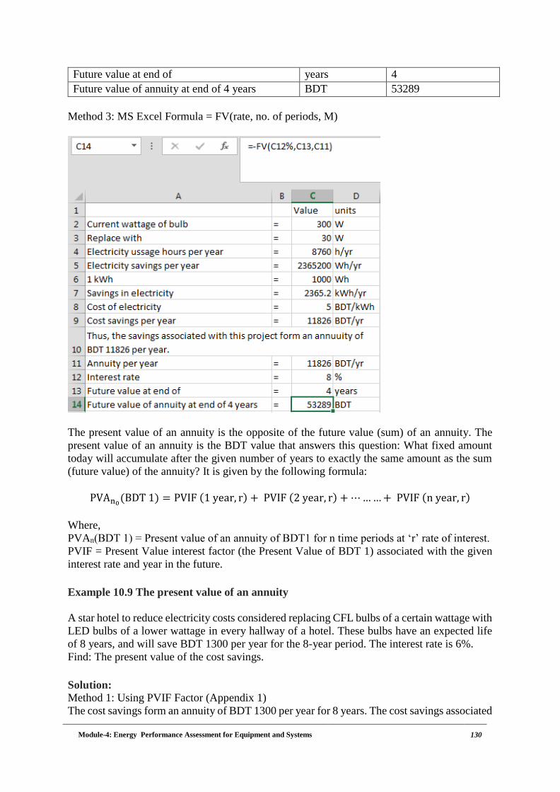
Module-4: Energy Performance Assessment for Equipment and Systems 130
Future value at end of years 4
Future value of annuity at end of 4 years BDT 53289
Method 3: MS Excel Formula = FV(rate, no. of periods, M)
The present value of an annuity is the opposite of the future value (sum) of an annuity. The
present value of an annuity is the BDT value that answers this question: What fixed amount
today will accumulate after the given number of years to exactly the same amount as the sum
(future value) of the annuity? It is given by the following formula:
PVAn0(BDT 1) = PVIF (1 year, r) + PVIF (2 year, r) + ⋯ … … + PVIF (n year, r)
Where,
PVAn(BDT 1) = Present value of an annuity of BDT1 for n time periods at ‘r’ rate of interest.
PVIF = Present Value interest factor (the Present Value of BDT 1) associated with the given
interest rate and year in the future.
Example 10.9 The present value of an annuity
A star hotel to reduce electricity costs considered replacing CFL bulbs of a certain wattage with
LED bulbs of a lower wattage in every hallway of a hotel. These bulbs have an expected life
of 8 years, and will save BDT 1300 per year for the 8-year period. The interest rate is 6%.
Find: The present value of the cost savings.
Solution:
Method 1: Using PVIF Factor (Appendix 1)
The cost savings form an annuity of BDT 1300 per year for 8 years. The cost savings associated

Module-4: Energy Performance Assessment for Equipment and Systems 131
with each year will be discounted @ 6% individually back to the present, and the sum will be
taken as shown in table below.
Year Cost Savings (BDT) PVIF Present value (BDT)
1 1300 0.9434 1226.42
2 1300 0.8900 1157
3 1300 0.8396 1091.48
4 1300 0.7921 1029.73
5 1300 0.7473 971.49
6 1300 0.7050 916.5
7 1300 0.6651 864.63
8 1300 0.6274 815.62
Present value of Annuity 8072.87
Method 2: Using MS Excel Formula:
However, in reality costs change annually so does savings leading to non-uniform/irregular
flow of cost savings. For example the cost of LED bulbs may reduce or cost of electricity may
rise annually. In such cases annuity is calculated by taking the sum of the present value of the
savings associated with each year.
Example 10.10 Present value of an Irregular flow cost savings
Modern retail stores prefer giving customer’s good shopping experience and offer choices to
see and feel the goods before purchasing. Accordingly a modern retail store conducting
business for 310days/yr (12 h/d, Monday through Saturday) in an area of 25000 ft2 floor space
illuminated its store using400 fixtures having four 40W bulbs in each fixture. To reduce
electricity costs while maintaining visual comfort the store was recommended to remove two
lamps from every other light fixture in store. The cost of electricity is BDT 5 per kWh and the
contract ensures the same cost for the next 5 years, after which it will increase to BDT 5.5 per
kWh. The relevant interest rate is 10%.
Find: The annual cost savings associated with this project, and the present value of these
savings over the next 10 years.
Solution:
Unit Value
Floor area of store ft2 25000
Business hours per year h/yr 3720
Total no. of light fixtures at store nos. 400
No. of bulbs in each fixture nos. 4

Module-4: Energy Performance Assessment for Equipment and Systems 132
Wattage of each bulb W 40
Cost of electricity for first 5 years BDT/kWh 5
Cost of electricity for next 5 years BDT/kWh 5.5
No. of fixtures where change is made nos 200
No. of lamps removed at each fixture nos 2
Electricity saved per fixture W 80
Watts conserved in store area W 16000 = 16KW
Amount of energy saved per year kWh/yr 59520
Cost savings for first 5 years BDT/y 297600
Cost savings for next 5 years BDT/y 327360
So, the savings of the project form an annuity of 297600/yr for first 5 years, followed by another
5 year annuity of 327360/yr. The present value of these cost savings may be determined by
finding the present value of the cost savings associated with each year (a series of fixed
amounts) and then taking their sum. This process is shown below.
Year Cost savings(BDT) PVIF (Appendix 1) Present Value(BDT)
1 297600 0.9091 270548
2 297600 0.8264 245937
3 297600 0.7513 223587
4 297600 0.6830 203261
5 297600 0.6209 184780
6 327360 0.5645 184795
7 327360 0.5132 168001
8 327360 0.4665 152713
9 327360 0.4241 138833
10 327360 0.3855 126197
These can be assessed using energy and economic efficiency and marginal analysis of cost and
savings as explained below.
Method 3: Using MS Excel Formula:

Module-4: Energy Performance Assessment for Equipment and Systems 133
10.5 Financial Analysis Techniques
For management to consider any energy project the overall costs of all possible alternatives
should be known and the project should save at least as much as it costs. Depending on the
complexity and level of investment the following techniques can be used.
The basic criteria for financial investment appraisal include:
Simple Payback- a measure of how long it will be before the investment makes money, and
how long the financing term needs to be
Return on Investment (ROI) and Internal Rate of Return (IRR)- measure that allow comparison
with other investment options
Net Present Value (NPV) and Cash Flow - measures that allow financial planning of the project
and provide the company with all the information needed to incorporate
Energy efficiency projects into the corporate financial system.
Initially, when you can identify no or low cost investment opportunities, this principle should
not be difficult to maintain. However, if your organization decides to fund a rolling program
of such investments, then over time it will become increasingly difficult for you to identify
opportunities, which conform to the principle. Before you'll reach this position, you need to
renegotiate the basis on which investment decisions are made.
It may require particular thoroughness to ensure that all the costs and benefits arising are taken
into account. As an approximate appraisal, simple payback (the total cost of the measure
divided by the annual savings arising from it expressed as years required for the original
investment to be returned) is a useful tool.
As the process becomes more sophisticated, financial criteria such as Discounted Cash Flow,
Internal Rate of Return and Net Present Value may be used. If you do not possess sufficient
financial expertise to calculate these yourself, you will need to ensure that you have access,
either within your own staff or elsewhere within the organization, to people who can employ
them on your behalf.
There are two quite separate grounds for arguing that, at least long after their payback periods.
Such measure does not need to be written off using fast discounting rates but can be regarded
as adding to the long term value of the assets. For this reason, short term payback can be an
inadequate yardstick for assessing longer term benefits. To assess the real gains from investing
in saving energy, you should use investment appraisal techniques, which accurately reflect the
longevity of the returns on particular types of technical measures.
10.5.1 Simple Pay Back Period
Simple Payback Period (SPP) represents, as a first approximation; the time (number of years)
required to recover the initial investment (First Cost), considering only the Net Annual Saving.
The annual net cost saving is the least savings achieved after all the operational costs have been
met. This is the simplest technique that can be used to appraise a proposal, despite its
limitations that it does not consider cash-flows after the payback period, which may be
substantial. Hence It can be considered as a metric to measure a project's capital recovery and
not profitability.
The simple payback period is usually calculated as follows:
Simple payback period (years) = Capital cost of the project (in BDT)
Net Annual Savings (in BDT)

Module-4: Energy Performance Assessment for Equipment and Systems 134
Example 10.11 Calculating pay-back period.
A new small cogeneration plant installation is expected to reduce a company's annual energy
bill by BDT 4, 86,000. If the capital cost of the new boiler installation is BDT22, 20,000 and
the annual maintenance and operating costs are BDT 42,000, the expected payback period for
the project can be worked out as follows.
Solution
Payback = 22,20,000
(4,86,000 − 42,000)= 5 years
According to the payback criterion, the shorter the payback period, the more desirable the
project
Example 10.12 Payback Period when savings each year are equal
A SME (Small and Medium scale enterprise) considered a desktop computer with energy
monitoring and management software to pursue energy conservation opportunities. The system
has an original cost of BDT 3, 20,000 and will generate net after tax savings of BDT 40,000
per year.
Find: The payback period of this investment
Solution:
𝑃𝑎𝑦𝑏𝑎𝑐𝑘 𝑝𝑒𝑟𝑖𝑜𝑑 = 𝐵𝐷𝑇 320000
𝐵𝐷𝑇 40000= 8 𝑦𝑒𝑎𝑟𝑠
If savings each year are not constant then the above equation is not applicable. In such case
savings from each year are added until their sum equals the original investment. An example
is shown below.
Example 10.13 Payback period when savings each year are not constant
In the above example (example 13)), suppose the annual net cost savings is BDT40,000 for the
first year will increase 12% each year thereafter, whereas, the original price of the system
remains at BDT 3,20,000.Find the payback period of this investment.
Solution: Consider the following table.
Year Original Savings
(first year)(BDT)
Escalation
FVIP 12%
Actual savings for
year(BDT)
Cumulative savings at end
of year(BDT)
0 40000 Given 40000 40000
1 40000 1.12 44800 84800
2 40000 1.2544 50176 134976
3 40000 1.4049 56196 191172
4 40000 1.5735 62940 254112
5 40000 1.7623 70492 324604
Table: Payback period with an irregular flow of cost savings

Module-4: Energy Performance Assessment for Equipment and Systems 135
The Table above shows, the total cost savings of the project become equal to its cost at the end
of the fifth year. Thus, a rough estimate of the payback period if 5 years.
Advantages
A widely used investment criterion, the payback period seems to offer the following
advantages:
It is simple, both in concept and application. Obviously a shorter payback generally indicates
a more attractive investment. It does not use tedious calculations.
It favors projects, which generate substantial cash inflows in earlier years, and discriminates
against projects, which bring substantial cash inflows in later years but not in earlier years.
Limitations
It fails to consider the time value of money. In the above example the net cost savings of 5th
year are counted equally with those of the first year. This violates the most basic principle of
financial analysis, which stipulates that cash flows occurring at different points of time can be
added or subtracted only after suitable compounding/discounting.
The payback method does not consider savings that are accrued after the payback period has
finished. This leads to discrimination against projects that generate substantial cash inflows in
later years.
Example 10.14 Understanding limitation of pay-back period
To consider impact of cash flows after the payback period is over, consider the cash flows of
two projects, A and B: The payback criterion prefers A, which has a payback period of 3 years,
in comparison to B, which has a payback period of 4 years, even though B has very substantial
cash inflows in years 5 and 6.
Investment/ Savings in
Year
Cash Flow of A (BDT) Cash Flow of B (BDT)
1 50,000 20,000
2 30,000 20,000
3 20,000 20,000
4 10,000 40,000
5 10,000 50,000
6 - 60,000
10.5.2 Return on Investment (ROI)
ROI expresses the "annual return" from the project as a percentage of capital cost. The annual
return takes into account the cash flows over the project life and the discount rate by converting
the total present value of ongoing cash flows to an equivalent annual amount over the life of
the project, which can then be compared to the capital cost. ROI does not require similar project
life or capital cost for comparison.
This is a broad indicator of the annual return expected from initial capital investment, expressed
as a percentage:
ROI = Annual Net Cash Flow
Capital Cost × 100

Module-4: Energy Performance Assessment for Equipment and Systems 136
Limitations
It does not take into account the time value of money.
It does not account for the variable nature of annual net cash in flows.
Example 10.15 Calculating rate of return
A municipality replaced 1000,40 W CFL street light bulbs with 25 W LED bulbs investing
BDT 30,00,000. The life of LED bulbs is 10 years. The annual electricity savings due to
replacement of bulbs is 65700 kWh considering 12 hrs operation. Assuming electricity cost of
BDT 5.0, annualized yearly savings are BDT 201849 considering interest rate of 10%. The
return on investment would be:
ROI = 201849
3000000 × 100 = 6.73%
10.5.3 Benefit-Cost Analysis
The net cost savings of an energy project are often called the benefits of the project. If the
actual net cost savings per year are identical and known, they can be used to compute the
benefit-cost ratio. The formula for this ratio is as follows:
Benefit
Cost=
Actual net cost savings yr⁄
Net cost savings yr needed to recover original investment⁄
If the benefit-cost ratio is larger than one, then the net cost savings of a project (or its benefits)
exceed its cost and the investment is profitable. If the ratio is less than one, then the net cost
savings needed per year are greater than those actually obtained and the investment is not
profitable.
10.5.4 Profitability index
Another technique, which can be used to evaluate the financial viability of projects, is the
profitability index. The profitability index can be defined as:
Profitability Index = Sum of the discounted net savings
Capital Costs
The higher the profitability index, the more attractive the project.
Example 10.16 Calculating and comparing profitability index of two different projects
Consider two projects A and B with investment of BDT 30,000 in project A and BDT 35000
in project B. The assessment of profits indicate project A generates profit of BDT 10,254 and
project B generates profit of BDT 10,867 over the life of project tenure. The profitability index
can be calculated as given below.
For Project A: Profitability index = 10,254
30,000= 0.342
For Project B: Profitability index = 10,867
33,000= 0.33

Module-4: Energy Performance Assessment for Equipment and Systems 137
Project A is therefore a better proposal than Project B.
This index is a quick tool to consider the better alternative among two different proposed
projects.
10.6 Discounted Cash Flow Methods
In order to overcome the weakness of simple pay-back assessment method a number of
discounted cash flow techniques have been developed, which are based on the fact that money
invested in a bank will accrue annual interest. If a fixed amount of money or a series of equal,
yearly cost savings (an-annuity) is associated with a certain time period, then an amount
associated with the present – which is equal to the future amount can be calculated. The latter
figure is the present value of the fixed amount, or the annuity. This process is called
discounting. The two most commonly used techniques are the 'net present value' and the
'internal rate of return' methods.
10.6.1 Net Present Value
Because an amount of money in the present is worth more than the same amount at any point
in the future due to time value of money, all amounts should be converted to the same period
to arrive at net present value. The net present value method achieves this by quantifying the
impact of time on any particular future cash flow. This is done by equating each future cash
flow to its current value today, in other words determining the present value of any future cash
flow. The present value (PV) is determined by using an assumed interest rate, usually referred
to as a discount rate. Discounting is the opposite process to compounding. Compounding
determines the future value of present cash flows, where" discounting determines the present
value of future cash flows. The net present value (NPV) of a project is equal to the sum of the
present values of all the cash flows associated with it. Symbolically,
NPV = CF0
(1 + k)0+
CF1
(1 + k)1+ . . . . . +
CFn
(1 + k)n= ∑
CFt
(1 + k)t
n
t=0
Where
NPV = Net Present Value
CFt = Cash flow occurring at the end of year 't' (t=0,1,….n) n = life of the project
k = Discount rate
The discount rate (k) employed for evaluating the present value of the expected future cash
flows should reflect the risk of the project.
Example 10.17 Calculating NPV
To illustrate the calculation of net present value, consider a project, which has the following
cash flow stream:
Investment/Savings year-wise Cash Flow (BDT)
1 200,000
2 200,000
3 300,000
4 300,000
5 350,000
The cost of capital, k, for the firm is 10 per cent. The net present value of the proposal is:

Module-4: Energy Performance Assessment for Equipment and Systems 138
NPV = − 1,000,000
(1.10)0+
200,000
(1.10)1+
200,000
(1.10)2+
300,000
(1.10)3+
300,000
(1.10)4+
350,000
(1.10)5= 5,273
Example 10.18 Calculating NPV
In a cement plant, 16000 liter lubricant/yr is used to manually lubricate grinding equipment
gear trains every 2 hours, using. An automatic oil-mist system was proposed by a supplier
claiming that his automatic system uses only 600liters/yr without compromising on lubricating
functionality. The gear lubricant costs BDT 100/liter. The expected life of the system is 5 years.
The system would cost BDT 6, 00,000 to purchase and install. Maintenance costs would be
BDT 37000/yr. The interest rate is 9%. Find the net present value of installing the automatic
oil-mist system.
Solution:
unit value
Current lubricant usage lit/yr 16000
Cost of lubricant BDT/lit 100
Lubricant required in new oil-mist system lit/yr 600
Life of new system yr 5
Capital cost of new system BDT 6,00,000
Maintenance cost of new system BDT/yr 37000
Interest rate % 9
Solution Lubricant savings due to new system lit/yr 15400
Cost savings BDT/yr 5,40,000
Thus, the cost savings associated with this project form an annuity of BDT 154000/yr for
5 years. The present value of this annuity is as follows:
PV(cost savings) BDT 59,90,063
PV(maintenance requirement) BDT 1,43,917
Present value of the purchase of installation and maintaining new system
PV(all costs of new system) BDT 7,43,917
Net Present Value (NPV) BDT 52,46,146
Since NPV > 0 the project should be implemented
Alternate method: net cost savings/yr (Savings – Cost) BDT/yr 1503000
Present value of net cost savings Net savings/yr x PVIFa (5 years, 9%)
BDT 5846146
Net Present value PVof(net cost savings - Capital cost)
BDT 5246146
When analyzing one particular project, the NPV methods offers no special advantage.
However, the NPV methods becomes most useful when a particular function can be performed
in more than one way.

Module-4: Energy Performance Assessment for Equipment and Systems 139
Example 10.19 Comparing NPV of different options
Example: Suppose that in Examples above, 4 different oil-mist systems were available at
differing costs, each system could reduce costs by a different amount, and each had a NPV
greater than zero (total cost savings exceed total costs in present-value terms).
Choice among alternative Oil-mist systems
System Capital Cost
(BDT)
Maintenance
cost (BDT/yr)
Cost Savings
(BDT) NPV (BDT)
1 4,00,000 60,000 10,00,000 32,56,272
2 5,00,000 55,000 12,00,000 39,53,651
3 5,50,000 45,000 15,00,000 51,09,443
4 6,00,000 25,000 15,00,000 51,37,236
In this example, System 4 would be implemented since it has the highest NPV. Once the
alternative ways of achieving a goal have been determined, the NPV method can be used to
choose from among the alternatives.
However, it is common practice to use a discount factor (DF) when calculating present value.
The discount factor is based on an assumed discount rate (i.e. interest rate) and can be
determined by using equation.
DF = (1 + IR
100)−n
The product of a particular cash flow and the discount factor is the present value.
PV = S × DF The values of various discount factors computed for a range of discount rates (i.e. interest rates)
are shown in the annexure-1.
Example 10.20 Evaluation of financial merits using NPV
Using the net present value analysis technique evaluate the financial merits of the proposed
projects shown in the table below assuming an annual discount rate of 8%.
Project A Project B
Capital cost in BDT 30,000 30,000
Year Net annual savings (BDT) Net annual savings (BDT)
1 6,000 6,600
2 6,000 6,000
3 6,000 6,300
4 6,000 6,300
5 6,000 6,000
6 6,000 6,000
7 6,000 5,700
8 6,000 5,700
9 6,000 5,400
10 6,000 5,400
Total net savings at the end of
year 10
60,000 60,000

Module-4: Energy Performance Assessment for Equipment and Systems 140
Solution
The annual cash flows should be multiplied by the annual discount factors for a rate of 8% to
determine the annual present values, as shown in the table below:
Formula: NPVBenefits = NPVSavings − Capital Cost
Year Discount Factor
for 8% (a)
Project A Project B
Net savings
(BDT) (b)
Present value
(BDT) (a*b)
Net savings
(BDT) (b)
Present value
(BDT) (a*b)
0 1.000 (30,000) (30,000) (30,000) (30,000)
1 0.926 6,000 5,556.00 6,600 6,111.60
2 0.857 6,000 5,142.00 6,000 5,656.20
3 0.794 6,000 4,764.00 6,300 5,002.20
4 0.735 6,000 4,410.00 6,300 4,630.50
5 0.681 6,000 4,086.00 6,000 4,086.00
6 0.630 6,000 3,780.00 6,000 3,780.00
7 0.583 6,000 3,498.00 5,700 3,323.10
8 0.540 6,000 3,240.00 5,700 3,078.00
9 0.500 6,000 3,000.00 5,400 2,700.00
10 0.463 6,000 2,778.00 5,400 2,500.20
NPV=10,254 NPV=10,868
Method 2: Using MS Excel
In Excel for each year PV is calculated according to formulas explained in earlier examples.
The sum of present values gives the NPV.
The net present value represents the net benefit over and above the compensation for time and
risk.
It can be seen that over a 10 year life-span the net present value of Project A is BDT 10,254,
while for Project B it is BDT 10,868. Therefore Project B is the preferential proposal.
Hence the decision rule associated with the net present value criterion is: "Accept the project
if the net present value is positive and reject the project if the net present value is negative".
Advantages
The net present value criterion has considerable merits.
It takes into account the time value of money.
It considers the cash flow stream in its project life.
Limitations
The whole credibility of the net present value method depends on a realistic prediction of future
interest rates, which can often be unpredictable. It is prudent therefore to set the discount rate
slightly above the interest rate at which the capital for the project is borrowed. This will ensure
that the overall analysis is slightly pessimistic, thus acting against the inherent uncertainties in
predicting future savings.

Module-4: Energy Performance Assessment for Equipment and Systems 141
10.6.2 Internal Rate of Return
This method calculates the rate of return that the investment is expected to yield. The internal
rate of return (IRR) method expresses each investment alternative in terms of a rate of return.
The expected rate of return is the interest rate for which total discounted benefits become just
equal to total discounted costs (i.e. net present benefits or net annual benefits are equal to zero,
or for which the benefit / cost ratio equals one). The criterion for selection among alternatives
is to choose the investment with the highest rate of return.
The discount rate which achieves a net present value of zero is known as the internal rate of
return (IRR) The higher the internal rate of return, the more attractive the project.
The rate of return is usually calculated by a process of trial and error, whereby the net cash
flow is computed for various discount rates until its value is reduced to zero and is calculated
using the equation given below.
0 = CF0
(1 + k)0+
CF1
(1 + k)1+ ⋯ … … … +
CFn
(1 + k)n= ∑
CFt
(1 + k)t
n
t=0
Where,
CFt cash flow at the end of year "t"
k discount rate
n life of the project
• CFt is negative if expenditure> savings
• CFt is positive if expenditure < savings.
In the net present value calculation we assume that the discount rate (cost of capital) is known
and determine the net present value of the project. In the internal rate of return calculation, we
set the net present value equal to zero and determine the discount rate (internal rate of return),
which satisfies this condition.
Example 10.21 Evaluate internal rate of return
To illustrate the calculation of internal rate of return, consider the cash flows of a project:
Year 0 1 2 3 4
Cash Flow (1,00,000) 30,000 30,000 40,000 45,000
The internal rate of return is the value of “K” which satisfies the following equation:
1,00,000 = 30,000
(1 + 𝑘)1+
30,000
(1 + 𝑘)2+
40,000
(1 + 𝑘)3+
45,000
(1 + 𝑘)4
The calculation of “K” involves a process of trial and error. We try different values of “K” till
we find that the right-hand side of the above equation is equal to 1, 00,000. Let us, to begin
with, try K-15 per cent. This makes the right-hand side equal to:
30,000
(1.15)+
30,000
(1.15)2+
40,000
(1.15)3+
45,000
(1.15)4= 1,00,802

Module-4: Energy Performance Assessment for Equipment and Systems 142
This value is slightly higher than our target value, 100,000. So we increase the value of k from
15 per cent to 16 per cent. (In general, a higher k lowers and a smaller k increases the right-
hand side value). The right-hand side becomes:
30,000
(1.16)+
30,000
(1.16)2+
40,000
(1.16)3+
45,000
(1.16)4= 98,641
Since this value is now less than 100,000, we conclude that the value of k lies between 15 per
cent and 16 per cent. For most of the purposes this indication suffices.
Example 10.22 Calculate the internal rate of return (IRR)
The manager of a warehouse is considering the installation of an air lock at the loading door.
The size of the door is 20 ft x 17.5 ft. The door is open for 10minutes -12 times a day – 5 days
per week. The inside building temperature is 70°F. The heating season is October – April (30
weeks). The average outside temperature during the heating season is 38.4°F. The air flow
velocity through the open door is 500 fpm. Steam, which supplies 2100 Btu/kg, is used for
heating. The cost of steam is BDT 0.5/kg. The cost of the air-lock is BDT 17,70,000 installed.
Assume the life of the air lock is 20 years.
Find the internal rate of return (IRR) of the purchase and installation cost of the air lock.
Use conversion factor: 0.0183 Btu = 1 ft3-°F.
Unit Value
Door size ft 20 x 17.5
Area of door ft2 350
Door opening time minutes 10
No. of times it is opened in a day nos 12
No .of days it is opened in a week nos 5
No. of weeks heating is required nos 30
Inside building temperature °F 70
Outside temperature °F 38.4
Air flow velocity fpm 500
Heat value of steam Btu/kg 2100
Cost of steam BDT/kg 0.5
0.0183Btu supplied to 1 ft3 air raises temp by 1°F ft3-°F 1
Cost of air lock installed BDT 17,00,000
Life of air lock years 20
Conversion factor BTU ft3 °F 0.0183
Solution: Air entering door ft3/min 175000
Temperature difference between inside and outside °F 31.6
Heat loss Btu/min 101199
Heating cost per min of door opening BDT/min 24.095
Annual cost savings due to installation of air lock BDT/yr 433710
Thus, this project yields uniform savings of BDT 433710/yr over its life.
Proper PVIa (20 years, ?%) 3.920
From Appendix 3, for 20 year period the proper PVIa of 3.92 corresponds to 25% interest
PVIa of 3.954 and26% interest PVIa of 3.808. Since the PVIa needed is equal to 3.920 the
exact value of internal rate of return (i)can be interpolated as follows.
i = 0.25 + (0.26-0.25) x 3.954 / (3.954 +3.808) = 0.255, or 25.5 percent

Module-4: Energy Performance Assessment for Equipment and Systems 143
Example 10.23 Assess project whether it will achieve desired IRR
A proposed project requires an initial capital investment of BDT 20,000. The cash flows
generated by the project are shown in the table below:
Year Cash flow (BDT)
0 (20,000)
1 6,000
2 5,500
3 5,000
4 4,500
5 4,000
6 4,000
Given the above cash flow data, let us find out the internal rate of return for the project.
Solution
Year Cash flow
(BDT)
8% discount rate 12% discount rate 16% discount rate
Discount
factor
Present
value (BDT)
Discount
factor
Present
value
(BDT)
Discount
factor
Present
value
(BDT)
0 (20,000) 1.000 (20,000) 1.000 (20,000) 1.000 (20,000)
1 6,000 0.926 5,560 0.893 5,358 0.862 5,172
2 5,500 0.857 4,713.5 0.797 4,383.5 0.743 4,086.5
3 5,000 0.794 3,970 0.712 3,560 0.641 3,205
4 4,500 0.735 3,307.5 0.636 2,862 0.552 2,484
5 4,000 0.681 2724 0.567 2,268 0.476 1,904
6 4,000 0.630 2520 0.507 2,028 0.410 1,640
NPV=2791 NPV=459.5 NPV=(1,508.5)
It can clearly be seen that the discount rate which results in the net present value being zero
lies somewhere between 12% and 16%.
For12% discount rate, NPV is positive; for 16% discount rate, NPV is negative. Thus, for some
discount rate between 12 and 16 percent, present value benefits are equated to present value
costs. To find the value exactly, one can interpolate between the two rates as follows:
Internal rate of return = 0.12 × (0.16 − 0.12) × 459.5
(459 − (−1,508.5)) × 100
Internal rate of return = 12.93%
Thus, the internal rate of return for the project is 12.93 %. At first sight both the net present
value and internal rate of return methods look very similar, and in some respects are. Yet there
is an important difference between the two. The net present value method is essentially a
comparison tool, which enables a number of projects to be compared, while the internal rate of
return method is designed to assess whether or not a single project will achieve a target rate of
return.

Module-4: Energy Performance Assessment for Equipment and Systems 144
Advantages
A popular discounted cash flow method, the internal rate of return criterion has several
advantages:
It takes into account the time value of money.
It considers the cash flow stream in its entirety.
It makes sense to businessmen who prefer to think in terms of rate of return and find an absolute
quantity, like net present value, somewhat difficult to work with.
Limitations
A central point of criticism of the IRR Method is the implicit reinvestment assumption, which
can lead to unrealistically high profitability rates. The IRR method should consequently be
backed by a NPV calculation.
Example 10.24 Calculate IRR based on project savings
Calculate the internal rate of return (i) for an economizer that will cost BDT 500,000, will last
10 years, and will result in fuel savings of BDT 150,000 each year. Find the ‘i’ that will equate
the following:
BDT 500,000 = 150,000 x PV (A = 10 years, i =?)
To do this,
Step I: Calculate proper PVIa
Proper PVIa = Cost
Annual savings =
500000
150000 = 3.33
From PVIa Table in Appendix 3, for 10 years period check PVIa values corresponding to proper
PVIa i.e., 3.33. As can be seen from PVIa table, the IRR falls between 27% and 28% with PVIa
of 3.364 and 3.269.
To find the rate more exactly, one can interpolate between the two rates as follows:
i = 0.27 + (0.28-0.27) x 3.364 / (3.364+3.269) = 0.275, or 27.5 percent
10.6.3 Modified Internal Rate of Return
Whenever the cost savings of an energy project are not the same each year, then the preceding
techniques cannot be used to determine IRR. The present value of the net cost savings of each
year should be discounted back to the present and summed, using various interest rates. That
interest rate, which leads to a total present value of net cost savings that is very close to the
original cost of the project, is the approximate internal rate of return.
In order to eradicate the limitation of the conventional IRR method, the modified IRR method
replaces the implicit reinvestment assumption with an explicit reinvestment rate. This method
requires an external project-unrelated investment opportunity rate. All positive future cash
flows are discounted with this external interest rate to acquire their respective present value.
Possible reinvestment rates are:
Average corporate return rate: Applicable in case the cash returns are invested in the operating
activities of accompany.
Achievable interest rate in the capital market: Cash returns are invested in the capital market.

Module-4: Energy Performance Assessment for Equipment and Systems 145
Loan interest rate: In case the cash returns are used to repay loans, the respective loan interest
rate should be used.
The MIRR is calculated as follows:
𝑰𝑹𝑹𝒎𝒐𝒅 = √∑ 𝑬𝒕 × (𝟏 + 𝒓𝑬𝑿𝑻)𝒏−𝒕 + 𝑹𝒏
𝒏𝒕=𝟏
∑ 𝑨𝒕 × (𝟏 + 𝒓𝑬𝑿𝑻)−𝒕𝒏𝒕=𝟎
− 𝟏𝒏
Where
IRRmod = modified Internal Rate of Return
At = negative Cash Flows at timed
Et = positive Cash Flows at timed
rEXT = reinvestment rate
n = operating life
Rn = remaining value at timed
Table 10.2: Comparison of Project Evaluation Methods
Method Needed Information Result
Capital recovery factor and
benefit-cost
Original cost;
Life of investment;
Relevant interest rate
Needed cost savings per year
to recover original
investment;
Ratio that shows how cost
savings relate to cost
Net Present value Original cost;
Life of investment;
Relevant interest rate;
Net cost savings per year
How much total present
value of net cost savings
exceeds (or less than)
original cost
Internal Rate of Return Original cost;
Life of net cost savings per
year
Interest rate which shows
how net cost savings relate to
original cost
Payback period Original cost;
Net cost savings per year
Rough estimate of time
needed to recover original
cost.

Module-4: Energy Performance Assessment for Equipment and Systems 146
Chapter 11: Sensitivity and Risk Analysis
Many of the cash flows in the project are based on assumptions that have an element of
uncertainty. The present day cash flows, such as capital cost, energy cost savings, maintenance
costs etc. can usually be estimated fairly accurately. Even though these costs can be predicted
with some certainty, it should always be remembered that they are only estimates. Cash flows
in future years normally contain inflation components which are often "guesstimates" at best.
The project life itself is an estimate that can vary significantly.
Sensitivity analysis is an assessment of risk. Because of the uncertainty in assigning values to
the analysis, it is recommended that a sensitivity analysis be carried out - particularly on
projects where the feasibility is marginal.
How sensitive is the project's feasibility to changes in the input parameters?
What if one or more of the factors in the analysis is not as favorable as predicted?
How much would it have to vary before the project becomes unviable?
What is the probability of this happening?
Suppose, for example, that a feasible project is based on an energy cost saving that escalates at
10% per year, but a sensitivity analysis shows the break-even is at 9% (i.e. the project becomes
unviable if the inflation of energy cost falls below 9%). There is a high degree of risk associated
with this project - much greater than if the break-even value was at 2%.
Many of the computer spreadsheet programs have built in "what if" functions that make
sensitivity analysis easy. If carried out manually, the sensitivity analysis can become laborious
- reworking the analysis many times with various changes in the parameters.
Sensitivity analysis is undertaken to identify those parameters that are both uncertain and for
which the project decision, taken through the NPV or IRR, is sensitive. Switching values
showing the change in a variable required for the project decision to change from acceptance
to rejection are presented for key variables and can be compared with post evaluation results
for similar projects.
For large projects and those close to the cut-off rate, a quantitative risk analysis incorporating
different ranges for key variables and the likelihood of their occurring simultaneously is
recommended. Sensitivity and risk analysis should lead to improved project design, with
actions mitigating against major sources of uncertainty being outlined
The various micro and macro factors that are considered for the sensitivity analysis are listed
below.
Micro factors
Operating expenses (various expenses items)
Capital structure
Costs of debt, equity
Changing of the forms of finance e.g. Leasing
Changing the project duration

Module-4: Energy Performance Assessment for Equipment and Systems 147
Macro factors
Macro-economic variables are the variable that affects the operation of the industry of which
the firm operates. They cannot be changed by the firm's management. Macro-economic
variables, which affect projects, include among others:
Changes in interest rates
Changes in the tax rates
Changes in the accounting standards e.g. methods of calculating depreciation
Changes in depreciation rates
Extension of various government subsidized projects e.g. extension of subsidies for
setting up industries in under-developed regions or subsidizing renewables use etc.
General employment trends e.g. improved employment conditions result in shortage of
skilled man-power and thereby increases their hiring costs and salaries.
Imposition of regulations on environmental and safety issues in the industry
Energy Price change
Technology changes
The sensitivity analysis will bring changes in various items in the analysis of financial
statements or the projects, which in turn might lead to different conclusions regarding the
implementation of projects.
11.1 Impact of interest rates on cash flows
In assessing likely interest out-go, it needs to be appreciated that interest rates charged may be
fixed or variable. For assessment purposes long time average rates may be considered. The
interest rate trend for Bangladesh is shown in figure below.
Figure 11.1: Lending Rate in Bangladesh
(Source: World Bank)
11.2 Impact of Depreciation rates on cash flows
In the above sections and examples the basic principles associated with the financial analysis
of projects were considered, but they do not consider the following important issues:
The capital value of plant and equipment generally depreciates overtime.
General inflation reduces the value of savings as time progresses. For example, BDT 1000
saved in 1 years’ time will be worth more than BDT 1000 saved in 10 years’ time.

Module-4: Energy Performance Assessment for Equipment and Systems 148
These issues are addressed by considering the income-relevant decrease of the value of the
investment called depreciation or amortization. While there are various methods available,
national legislations usually dictate the method to be used to determine amortization and
depreciation expenses. Knowledge of legislated depreciation rates may help in minimizing tax
outflows, for example accelerated depreciation is allowed for energy efficient or clean energy
products or technologies. The most commonly used methods to calculate depreciation are as
follows.
Straight line method
Reducing balance method
Sum of years depreciation method
Units of production depreciation method
11.2.1 Straight-line Depreciation
Straight-line depreciation is the simplest and most common type of depreciation. It is calculated
by dividing the initial asset value of the investment by its operating lifetime. The depreciation
amount is consequently identical for every period.
Depreciation Amount = Initial Value of Asset
Operating Lifetime
Example 11.1 Calculate straight-line depreciation
Consider a pump which is purchased at BDT 10,000 and has a life of 5 years. Calculate
the schedule of depreciation using straight line depreciation method.
Depreciation Amount = 10000
5 = 2000
The pump depreciates by BDT 2000 every year for 5 years. The schedule of depreciation
can be tabulated as follows:
Year Depreciation Amount Remaining Value
0 0 10,000
1 2,000 8,000
2 2,000 6,000
3 2,000 4,000
4 2,000 2,000
5 2,000 0
11.2.2 Reducing-balance Depreciation
The reducing-balance depreciation is characterized by declining depreciation amounts over the
duration of an asset’s operating lifetime. This is due to depreciation ensues with a constant
percentage rate. Depreciation amounts are calculated as follows:
Depreciation amount= Depreciation rate * Remaining value of the previous year

Module-4: Energy Performance Assessment for Equipment and Systems 149
Example 11.2 Calculate reducing-balance depreciation
Consider a pump which is purchased at BDT 10,000 and has a life of 5 years and depreciates
at a fixed rate of 30% every year. Calculate the schedule of depreciation.
Year Depreciation Amount (BDT)
( = 0.3 x Remaining value of previous year)
Remaining
Value (BDT)
0 0 10,000
1 3,000 7,000
2 2,100 4,900
3 1,470 3,430
4 1,029 2,401
5 720 1,681
This approach would never reach a remaining value of zero. Therefore, it is common to switch
to straight-line depreciation by the time the depreciation amount of the reducing- balance
method drops below the depreciation amount of the straight-line method.
Example 11.3 Assessing when to switch to straight-line method from reducing balance
method of depreciation.
Consider a pump which is purchased at BDT 10,000 and has a life of 5 years and depreciates
at a fixed rate of 30% every year. Calculate the schedule of depreciation.
Step I: Calculate depreciation value by both methods as given in Table below:
Year
Straight – Line method Reducing balance method
Depreciation
Amount
Remaining
Value
Depreciation
Amount
Remaining
Value
0 0 10,000 0 10,000
1 2000 8,000 3,000 7,000
2 2000 6,000 2,100 4,900
3 2000 4,000 1,633 3,267
4 2000 2,000 1,633 1,633
5 2000 0 1,633 0
Step II: Check the year in which depreciation amount by reducing-balance method falls below
the straight-line value.
As can be seen, in year 3 the depreciation amount of the straight-line method (4,900/3 =1,633)
which exceeds the reducing-balance amount (1,470).
Step III: From the year in which the depreciation amount by reducing-balance method falls
below the straight-line value, consider depreciation by straight-line method.
Hence, in the above example, the last three years are depreciated by straight-line method.
11.2.3 Sum of Years Depreciation
Like the previously presented depreciation method, the sum of years depreciation method
results in higher depreciation amounts in the early years of an asset. A year’s respective
depreciation amount is calculated by dividing the total remaining years by the sum of years of
operating lifetime and multiplying it with initial asset value. In year three, this would

Module-4: Energy Performance Assessment for Equipment and Systems 150
consequently be
Depreciation amount (year 3) = 3
1 + 2 + 3 + 4 + 5 × initial Asset Value
Example 11.4 Calculate depreciation based on sum of years method
Year Assessment Method Depreciation
Amount
Remaining
Value
0 0
(1 + 2 + 3 + 4 + 5)× 10000
0 10,000
1 =
5
(1 + 2 + 3 + 4 + 5)× 10000
3,333 6,667
2 =
4
(1 + 2 + 3 + 4 + 5)× 10000
2,667 4,000
3 =
3
(1 + 2 + 3 + 4 + 5)× 10000
2,000 2,000
4 =
2
(1 + 2 + 3 + 4 + 5)× 10000
1,333 667
5 =
1
(1 + 2 + 3 + 4 + 5)× 10000
667 0
11.2.4 Units of Production Depreciation
In this depreciation method the value of the asset is decreased according to the actual usage of
the asset. In order to fully depreciate an asset, a total production output has to be presumed.
The annual depreciation amounts are calculated as follows:
Depreciation amount (year X) = Units produced (year X)
Total production output × Initial Asset Value
Example 5 Calculate depreciation based on rate of production
It is assumed that an asset with an initial value of 10,000 monetary units will have a total
lifetime output of 24,000 units.
Step I: Consider units produced in a particular year
Step II: Calculate ratio of units produced to total lifetime output
Step II: Multiply the ratio with initial value of asset
Year Production Units Depreciation Amount Remaining Value
0 0 10,000
1 6,000 2,500 7,500
2 6,000 2,500 5,000
3 5,000 2,083 2,917
4 4,000 1,667 1,250
5 3,000 1,250 0
The capital depreciation of an item of equipment can be considered in terms of its salvage value

Module-4: Energy Performance Assessment for Equipment and Systems 151
at the end of the analysis period. The Example 10.8 illustrates the point.
Example 11.6 Assessing impact of Salvage Value on NPV
It is proposed to install a heat recovery equipment in a factory. The capital cost of installing
the equipment is BDT 20,000 and after 5 years its salvage value is BDT 1500. The savings
accrued by the heat recovery device are as shown below. Calculate the net present value after
5 years with and without considering salvage value. Assume discount rate to be 8%.
Savings accrued
Year 1 2 3 4 5
Savings (BDT) 7000 6000 6000 5000 5000
Solution
Year Discount Factor for
8% (a)
Capital investment
(BDT) (b)
Net savings
(BDT)
(c)
Present value
(BDT) (a)*(b+c)
0 1.000 (20,000) (20,000)
1 0.926 7,000 6,482
2 0.857 6,000 5,142
3 0.794 6,000 4,764
4 0.735 5,000 3,675
5 0.681 1,500 5,000 4,426.5
NPV=4489.5
It is evident that over a 5-year life span the net present value of the project is BDT 4489.50.
Had the salvage value of the equipment not been considered, the net present value of the project
would have been only BDT 3468.00.
11.3 Changes in inflation rates: Real value
Inflation can be defined as the rate of increase in the average price of goods and services. In
some countries, inflation is expressed in terms of the retail price index (RPI), which is
determined centrally and reflects average inflation over a range of commodities. Because of
inflation, the real value of cash flow decreases with time. The real value of sum of money (S)
realized in n years’ time can be determined using the equation.
RV = S × (1 + R
100)−n
Where
RV real value of S realized in n years’ time
S value of cash flow in n years’ time
R inflation rate(%)
As with the discount factor, it is common practice to use an inflation factor when assessing the
impact of inflation on a project. The inflation factor can be determined using the equation.
Inflation Factor, IF = (1 + R
100)−n
The product of a particular cash flow and inflation factor is the real value of the cash flow.
RV = S × IF The application of inflation factors is considered in Example 10.9.

Module-4: Energy Performance Assessment for Equipment and Systems 152
Example 11.7 Calculate and assess impact of inflation on NPV of project
Recalculate the net present value of the energy recovery scheme in Example 11.3, assuming
the discount rate remains at 8% and the rate of inflation is 5%.
Solution:
Because of inflation;
Real interest rate = Discount Rate − Rate of inflation Therefore Real interest rate = 8 – 5 = 3%
Year Capital investment
(BDT)
Net savings
(BDT)
Real Discount
Factor for3% Present value (BDT)
0 (20,000) 1.000 (20,000)
1 7,000 0.971 6,471
2 6,000 0.943 5,132
3 6,000 0.915 4,743
4 5,000 0.888 3,654
5 1,500 5,000 0.863 4,398
NPV=4,398
When inflation is not considered the NPV is BDT 4489.5 (ref Example 11.3) and if inflation is
considered the NPV is BDT 4,398 demonstrating the depreciation of money value due to
inflation.
11.4 Considering Taxes in Financing and Investment
In making investment calculations, the previous elaboration has completely ignored tax issues.
In practice, taxes influence the profitability of investments and consequently need to be
considered when taking an investment decision.
From the perspective of a company, taxes represent out payments that need to be considered in
the cash flows. Taxes can be income-independent and –dependent.
Income-independent taxes: These taxes are usually property and consumer taxes. They
can be easily included with the other operational out-payments. While value- added
taxes are income-independent taxes as well, they are neglected in financing and
investment as it represents a pass-through item.
Income-dependent taxes: These taxes are corporate or income taxes, reducing the cash
return of an investment. Essential for the determination of the level of the income-
dependent taxes are not the return cash flows but the profit or loss before taxes, which
has to be multiplied by the tax rate to find out the required tax payment.
In order to determine the payable income tax of an investment opportunity, taxable profits have
to be estimated for every year of operating life by reducing taxable sales by taxable relevant
operating expenses. The latter includes cash expenses like staff and material costs and non-
cash expenses like depreciation and amortization. In case debt capital is utilized in financing
an investment opportunity, interest obligations have to be considered as well.
The forecast of income-dependent payable taxes is problematic, because the respective tax rate
may change over the operating life of an investment due to changes in the political framework
as can be seen from the corporate tax rates shown in figure below. The effort for determining
payable taxes precisely must consequently be assessed as disproportionately. Thus, investment
calculation usually resorts to the simplified specification of payables taxes.

Module-4: Energy Performance Assessment for Equipment and Systems 153
Figure 11.2: Corporate Tax Rate: Bangladesh
(Source: tradingeconomics.com, National Board of Revenue (NBR), Bangladesh)
While the overall corporate tax rate can be considered for preliminary assessment of tax
liability there is a need for informing themselves on tax rates that may vary with type of product
(Eg: Tax on revenue from renewable power could be less), the scale of industry (Eg: Micro,
Small and Medium industries may be given tax preference), market segment for the product
(Eg: exports or priority industrial sectors (eg: textile industries) may be taxed less owing to
their capacity to earn foreign exchange or generate employment) etc. Hence, it is important to
understand and assess tax liability before any investment not only to arrive at real rate of returns
but maximize returns utilizing tax exemptions if allowed.
In calculating taxes normally expenses are deducted from the gross revenue earned. After
deducting the applicable expenses depending on the tax rate specified for the industry/product,
the taxable amount is calculated by multiplying earnings after deductible expenses with the
applicable tax rate.
Example 11.8 Calculate income tax expenses
Consider a unit with an asset price of 10,000 BDT with an operating lifetime of 5 years and a
corporate tax rate of 30 percent. The unit follows the straight-line depreciation method. It is
assumed that the project is financing entirely with debt capital at an interest rate of 5 percent.
The principal repayment is done uniformly across the life of unit. The operating income
generated and expenses incurred are given in table below.
Year 1 Year 2 Year 3 Year 4 Year 5
Operating income 8,500 9,000 9,500 10,000 10,500
Operating expenses -1,000 -1,200 -1,400 -1,600 -1,800
Develop an income statement showing depreciation, interest and tax calculations.
EBITDA = Operating income − Operating Expenses
Depreciation Expenses = Initial Value of Asset
Operating Lifetime=
10000
5= 2000
EBIT = EBITDA − Depreciation Expenses
Interest Expenses = Remaining Assest value × interest rate
Remaining Asset Value = Asset Value in previous year − Yearly Depreciation

Module-4: Energy Performance Assessment for Equipment and Systems 154
EBT = EBIT − Interest Expenses
Income tax expenses = EBIT × income tax rate
EAT = EBT − Income Tax expenses
Using the above formulae, construct the income statement as given below to assess tax
liabilities.
Year 1 Year 2 Year 3 Year 4 Year 5
Operating income 8,500 9,000 9,500 10,000 10,500
Operating expenses -1,000 -1,200 -1,400 -1,600 -1,800
EBITDA ( A-B) 7,500 7,800 8,100 8,400 8,700
Depreciation expenses -2,000 -2,000 -2,000 -2,000 -2,000
EBIT 5,500 5,800 6,100 6,400 6,700
Interest expenses -500 -400 -300 -200 -100
EBT 5,000 5,400 5,800 6,200 6,600
Income tax expense -1,500 -1,620 -1,740 -1,860 -1,980
EAT 3,500 3,780 4,060 4,340 4,620
11.5 Impact of taxes on cash flows
As can be seen from the above example taxes impact returns. The net impact of taxes on returns
again can be assessed using the net present value concept. This is illustrated using the previous
example.
Example 11.9 Assessing impact of taxes on NPV of cash flows
Year
Discount factor
(10%) (a)
(Appendix 6)
Cash Flow after
Taxes (b)
(EAT)
Net Present
Value after
Taxes (a*b)
Cash Flow
before Taxes
(c) (EBT)
Net Present
Value before
Taxes (a*c)
0 1.000 -10,000 -10,000 -10,000 -10,000
1 0.909 3,500 3,182 5,000 4,545
2 0.826 3,780 3,124 5,400 4,463
3 0.751 4,060 3,050 5,800 4,358
4 0.683 4,340 2,964 6,200 4,235
5 0.621 4,620 2,869 6,600 4,098
NPV= 5,189 NPV= 11,699
It can be seen that payable taxes have a considerable effect on the profitability of the project.
In practice, the assessment of investment opportunities must be made after due consideration
of income tax expenses.
11.6 Impact of Different Depreciation Methods and taxation on Cash flows
The type of depreciation method has a considerable impact on the resulting profitability of a
project as well. Example 16 (Chapter 10) compares the Cash Flow after Taxes by using straight-
line depreciation with the Cash Flow after Taxes by using reducing-balance (see Example 11
of Chapter 10). Due to the higher depreciation expenses in the earlier periods, the respective
payable taxes are reduced and the first actual cash returns are increased by the latter method.

Module-4: Energy Performance Assessment for Equipment and Systems 155
Thus, because of the time value of money, the project would be more profitable with reducing-
balance depreciation. As a consequence, besides considering taxes, presented possible tax
investment incentives have to be investigated.
Example 11.10 Impact of depreciation and income taxes on NPV of cash flows.
Year Discount factor
(10%) (a)
Cash Flow after
Taxes (straight-
line) (b)
Net Present
Value after
Taxes (a*b)
Cash Flow after
Taxes
(Reducing-
balance) (c)
Net Present
Value after
Taxes (a*c)
0 1.000 -10,000 -10,000 -10,000 -10,000
1 0.909 3,500 3,182 3,800 3,455
2 0.826 3,780 3,124 3,810 3,149
3 0.751 4,060 3,050 3,950 2,968
4 0.683 4,340 2,964 4,230 2,889
5 0.621 4,620 2,869 4,510 2,800
NPV= 5,189 NPV= 5,260

Module-4: Energy Performance Assessment for Equipment and Systems 156
Chapter 12: Financing Options
Most high budget projects involve seeking external finances while smaller projects can be
funded by internal revenues. While financial viability assessments methods remain the same
for both external financing agencies may scrutinize the project more deeply to assess the
viability. Also, external financing agencies may conduct deeper sensitivity analysis to assess
risks before funding. The higher the risk normally the charges for financing will be higher.
Also, as per the mandate of the financing agencies they may fund projects preferentially (Eg:
Government supported or credit guaranteed projects may get preference). High risk projects
may not be financed by banks but by venture funds who look for higher returns. A project
proponent needs to be aware of these aspects and may include financing agencies likely to fund
the proposed project in their proposals.
The various options for financing energy management projects.
For projects requiring external funding
By obtaining a bank loan
By raising money from stock market
By awarding the project to Energy Service Company(ESCO)
For projects funded from internal resources:
From a central budget
From a specific departmental or section budget such as engineering
By retaining a proportion of the savings achieved.
While procedures for seeking funding from banks as loans or from stock markets as equity are
well established ESCOs and performance contracting have emerged as new tools that reduces
the risks of considering an energy efficiency or conservation project. Hence, implementing
energy saving projects using ESCOs and performance contracting methods are only
considered.
12.1 Energy Performance Contracting and Role of ESCOS
If the project is to be financed externally, one of the attractive options for many organizations
is the use of energy performance contracts delivered by energy service companies, or ESCOs.
ESCOs are usually companies that provide a complete energy project service, from assessment
to design to construction or installation, along with engineering and project management
services, and financing. In one way or another, the contract involves the capitalization of all of
the services and goods purchased, and repayment out of the energy savings that result from the
project.
In performance contracting, an end-user (such as an industry, institution, or utility), seeking to
improve its energy efficiency, contracts with ESCO for energy efficiency services and
financing.
In some contracts, the ESCOs provide a guarantee for the savings that will be realized, and
absorbs the cost if real savings fall short of this level. Typically, there will be a risk management
cost involved in the contract in these situations. Insurance is sometimes attached, at a cost, to
protect the ESCO in the event of savings shortfall.
Energy efficiency projects generate incremental cost savings as opposed to incremental
revenues from the sale of outputs. The energy cost savings can be turned into incremental cash

Module-4: Energy Performance Assessment for Equipment and Systems 157
flows to the lender or ESCO based on the commitment of the energy user (and in some cases,
a utility) to pay for the savings.
12.1.1 What are performance contracts?
Performance contracting represents one of the ways to address several of the most frequently
mentioned barriers to investment. Performance contracting through an ESCO transfers the
technology and management risks away from the end-user to the ESCO.
For energy users reluctant to invest in energy efficiency, a performance contract can be a
powerful incentive to implement a project. Performance contracting also minimizes or
eliminates the up-front cash outlay required by the end-user. Payments are made over time as
the energy savings are realized.
Figure 12.1
End-User
ESCO
Fund or Financial
Intermediary
Investment Agreement
Variable
performance – or
savings- based
energy payments
Provision of
engineering,
turnkey equipment
installation and
monitoring services
Provision of capital
for project costs
What is Performance Contracting?
The core of performance contracting is an agreement involving a comprehensive package of
services provided by an ESCO, including:
An energy efficiency opportunity analysis
Project development
Engineering
Financing
Construction/ Implementation
Training
Monitoring and Verification
Monitoring and verification, is key to the successful involvement of an ESCO in performance
contracting where energy cost savings are being guaranteed.
ESCOs are not “bankers” in the narrow sense. Their strength is in putting together a package
of services that can provide guaranteed and measurable energy savings that serve as the basis
for guaranteed cost savings. But, the energy savings must be measurable. Figure above shows
ESCO role.

Module -6: Energy Performance Assessment ©2018 AIP NPC, Chennai 158
12.2 Self-Financing Energy Management
Large and capital intensive energy savings project funding or implementation are considered based on
external financing smaller or easily implementable projects are considered by internal teams. To sustain
continuous improvement the teams need to be encouraged and funding mechanism for systematically
assessed viable projects needs to be created.
One way to make energy management self-financing is to split savings to provide identifiable returns to
each interested party. This has the following benefits:
Assigning a proportion of energy savings to your energy management budget means you have a
direct financial incentive to identify and quantify savings arising from your own activities.
Separately identified returns will help the constituent parts of your organization understanding
whether they are each getting good value for money through their support for energy management.
If operated successfully, splitting the savings will improve motivation and commitment to energy
management throughout the organization since staff at all levels will see a financial return for their
effort or support.
But the main benefit is on the independence and longevity of the energy management function.
12.3 Ensuring Continuity
After implementation of energy savings, your organization ought to be able to make considerable savings
at little cost (except for the funding needed for energy management staff). The important question is what
should happen to these savings?
If part of these easily achieved savings is not returned to your budget as energy manager, then your access
to self-generated investments funds to support future activities will be lost. And later in the program, it is
likely to be much harder for you to make savings.
However, if, an energy manager has access to a proportion of the revenue savings arising from staff's
activities, then these can be reinvested in:
Further energy efficiency measures
Activities necessary to create the right climate for successful energy management which do not, of
themselves, directly generate savings
Maintaining or up-grading the management information system.

Module -6: Energy Performance Assessment ©2018 AIP NPC, Chennai 159
APPENDIX 1 Present Value Tables
Discount factors: Present value of BDT1 to be received after t years = 1/(1 + r)t.
Number
of Years
Interest Rate per
Year
1% 2% 3% 4% 5% 6% 7% 8% 9% 10% 11% 12% 13% 14% 15%
1 .990 .980 .971 .962 .952 .943 .935 .926 .917 .909 .901 .893 .885 .877 .870
2 .980 .961 .943 .925 .907 .890 .873 .857 .842 .826 .812 .797 .783 .769 .756
3 .971 .942 .915 .889 .864 .840 .816 .794 .772 .751 .731 .712 .693 .675 .658
4 .961 .924 .888 .855 .823 .792 .763 .735 .708 .683 .659 .636 .613 .592 .572
5 .951 .906 .863 .822 .784 .747 .713 .681 .650 .621 .593 .567 .543 .519 .497
6 .942 .888 .837 .790 .746 .705 .666 .630 .596 .564 .535 .507 .480 .456 .432
7 .933 .871 .813 .760 .711 .665 .623 .583 .547 .513 .482 .452 .425 .400 .376
8 .923 .853 .789 .731 .677 .627 .582 .540 .502 .467 .434 .404 .376 .351 .327
9 .914 .837 .766 .703 .645 .592 .544 .500 .460 .424 .391 .361 .333 .308 .284
10 .905 .820 .744 .676 .614 .558 .508 .463 .422 .386 .352 .322 .295 .270 .247
11 .896 .804 .722 .650 .585 .527 .475 .429 .388 .350 .317 .287 .261 .237 .215
12 .887 .788 .701 .625 .557 .497 .444 .397 .356 .319 .286 .257 .231 .208 .187
13 .879 .773 .681 .601 .530 .469 .415 .368 .326 .290 .258 .229 .204 .182 .163
14 .870 .758 .661 .577 .505 .442 .388 .340 .299 .263 .232 .205 .181 .160 .141
15 .861 .743 .642 .555 .481 .417 .362 .315 .275 .239 .209 .183 .160 .140 .123
16 .853 .728 .623 .534 .458 .394 .339 .292 .252 .218 .188 .163 .141 .123 .107
17 .844 .714 .605 .513 .436 .371 .317 .270 .231 .198 .170 .146 .125 .108 .093
18 .836 .700 .587 .494 .416 .350 .296 .250 .212 .180 .153 .130 .111 .095 .081
19 .828 .686 .570 .475 .396 .331 .277 .232 .194 .164 .138 .116 .098 .083 .070
20 .820 .673 .554 .456 .377 .312 .258 .215 .178 .149 .124 .104 .087 .073 .061
Number
of Years
Interest Rate per
Year
16% 17% 18% 19% 20% 21% 22% 23% 24% 25% 26% 27% 28% 29% 30%
1 .862 .855 .847 .840 .833 .826 .820 .813 .806 .800 .794 .787 .781 .775 .769
2 .743 .731 .718 .706 .694 .683 .672 .661 .650 .640 .630 .620 .610 .601 .592
3 .641 .624 .609 .593 .579 .564 .551 .537 .524 .512 .500 .488 .477 .466 .455
4 .552 .534 .516 .499 .482 .467 .451 .437 .423 .410 .397 .384 .373 .361 .350
5 .476 .456 .437 .419 .402 .386 .370 .355 .341 .328 .315 .303 .291 .280 .269
6 .410 .390 .370 .352 .335 .319 .303 .289 .275 .262 .250 .238 .227 .217 .207
7 .354 .333 .314 .296 .279 .263 .249 .235 .222 .210 .198 .188 .178 .168 .159
8 .305 .285 .266 .249 .233 .218 .204 .191 .179 .168 .157 .148 .139 .130 .123
9 .263 .243 .225 .209 .194 .180 .167 .155 .144 .134 .125 .116 .108 .101 .094
10 .227 .208 .191 .176 .162 .149 .137 .126 .116 .107 .099 .092 .085 .078 .073
11 .195 .178 .162 .148 .135 .123 .112 .103 .094 .086 .079 .072 .066 .061 .056
12 .168 .152 .137 .124 .112 .102 .092 .083 .076 .069 .062 .057 .052 .047 .043
13 .145 .130 .116 .104 .093 .084 .075 .068 .061 .055 .050 .045 .040 .037 .033
14 .125 .111 .099 .088 .078 .069 .062 .055 .049 .044 .039 .035 .032 .028 .025
15 .108 .095 .084 .074 .065 .057 .051 .045 .040 .035 .031 .028 .025 .022 .020
16 .093 .081 .071 .062 .054 .047 .042 .036 .032 .028 .025 .022 .019 .017 .015
17 .080 .069 .060 .052 .045 .039 .034 .030 .026 .023 .020 .017 .015 .013 .012
18 .069 .059 .051 .044 .038 .032 .028 .024 .021 .018 .016 .014 .012 .010 .009
19 .060 .051 .043 .037 .031 .027 .023 .020 .017 .014 .012 .011 .009 .008 .007
20 .051 .043 .037 .031 .026 .022 .019 .016 .014 .012 .010 .008 .007 .006 .005
Note: For example, if the interest rate is 10% per year, the present value of BDT1 received at year 5 is
BDT.621.

Module -6: Energy Performance Assessment ©2018 AIP NPC, Chennai 160
APPENDIX 2 Future Value Tables
Future value of BDT1 after t years = (1 + r)t.
Number
of Years
Interest Rate per Year
1% 2% 3% 4% 5% 6% 7% 8% 9% 10% 11% 12% 13% 14% 15%
1 1.010 1.020 1.030 1.040 1.050 1.060 1.070 1.080 1.090 1.100 1.110 1.120 1.130 1.140 1.150
2 1.020 1.040 1.061 1.082 1.102 1.124 1.145 1.166 1.188 1.210 1.232 1.254 1.277 1.300 1.323
3 1.030 1.061 1.093 1.125 1.158 1.191 1.225 1.260 1.295 1.331 1.368 1.405 1.443 1.482 1.521
4 1.041 1.082 1.126 1.170 1.216 1.262 1.311 1.360 1.412 1.464 1.518 1.574 1.630 1.689 1.749
5 1.051 1.104 1.159 1.217 1.276 1.338 1.403 1.469 1.539 1.611 1.685 1.762 1.842 1.925 2.011
6 1.062 1.126 1.194 1.265 1.340 1.419 1.501 1.587 1.677 1.772 1.870 1.974 2.082 2.195 2.313
7 1.072 1.149 1.230 1.316 1.407 1.504 1.606 1.714 1.828 1.949 2.076 2.211 2.353 2.502 2.660
8 1.083 1.172 1.267 1.369 1.477 1.594 1.718 1.851 1.993 2.144 2.305 2.476 2.658 2.853 3.059
9 1.094 1.195 1.305 1.423 1.551 1.689 1.838 1.999 2.172 2.358 2.558 2.773 3.004 3.252 3.518
10 1.105 1.219 1.344 1.480 1.629 1.791 1.967 2.159 2.367 2.594 2.839 3.106 3.395 3.707 4.046
11 1.116 1.243 1.384 1.539 1.710 1.898 2.105 2.332 2.580 2.853 3.152 3.479 3.836 4.226 4.652
12 1.127 1.268 1.426 1.601 1.796 2.012 2.252 2.518 2.813 3.138 3.498 3.896 4.335 4.818 5.350
13 1.138 1.294 1.469 1.665 1.886 2.133 2.410 2.720 3.066 3.452 3.883 4.363 4.898 5.492 6.153
14 1.149 1.319 1.513 1.732 1.980 2.261 2.579 2.937 3.342 3.797 4.310 4.887 5.535 6.261 7.076
15 1.161 1.346 1.558 1.801 2.079 2.397 2.759 3.172 3.642 4.177 4.785 5.474 6.254 7.138 8.137
16 1.173 1.373 1.605 1.873 2.183 2.540 2.952 3.426 3.970 4.595 5.311 6.130 7.067 8.137 9.358
17 1.184 1.400 1.653 1.948 2.292 2.693 3.159 3.700 4.328 5.054 5.895 6.866 7.986 9.276 10.76
18 1.196 1.428 1.702 2.026 2.407 2.854 3.380 3.996 4.717 5.560 6.544 7.690 9.024 10.58 12.38
19 1.208 1.457 1.754 2.107 2.527 3.026 3.617 4.316 5.142 6.116 7.263 8.613 10.20 12.06 14.23
20 1.220 1.486 1.806 2.191 2.653 3.207 3.870 4.661 5.604 6.727 8.062 9.646 11.52 13.74 16.37
Number
of Years
Interest Rate per Year
16% 17% 18% 19% 20% 21% 22% 23% 24% 25% 26% 27% 28% 29% 30%
1 1.160 1.170 1.180 1.190 1.200 1.210 1.220 1.230 1.240 1.250 1.260 1.270 1.280 1.290 1.300
2 1.346 1.369 1.392 1.416 1.440 1.464 1.488 1.513 1.538 1.563 1.588 1.613 1.638 1.664 1.690
3 1.561 1.602 1.643 1.685 1.728 1.772 1.816 1.861 1.907 1.953 2.000 2.048 2.097 2.147 2.197
4 1.811 1.874 1.939 2.005 2.074 2.144 2.215 2.289 2.364 2.441 2.520 2.601 2.684 2.769 2.856
5 2.100 2.192 2.288 2.386 2.488 2.594 2.703 2.815 2.932 3.052 3.176 3.304 3.436 3.572 3.713
6 2.436 2.565 2.700 2.840 2.986 3.138 3.297 3.463 3.635 3.815 4.002 4.196 4.398 4.608 4.827
7 2.826 3.001 3.185 3.379 3.583 3.797 4.023 4.259 4.508 4.768 5.042 5.329 5.629 5.945 6.275
8 3.278 3.511 3.759 4.021 4.300 4.595 4.908 5.239 5.590 5.960 6.353 6.768 7.206 7.669 8.157
9 3.803 4.108 4.435 4.785 5.160 5.560 5.987 6.444 6.931 7.451 8.005 8.595 9.223 9.893 10.60
10 4.411 4.807 5.234 5.695 6.192 6.728 7.305 7.926 8.594 9.313 10.09 10.92 11.81 12.76 13.79
11 5.117 5.624 6.176 6.777 7.430 8.140 8.912 9.749 10.66 11.64 12.71 13.86 15.11 16.46 17.92
12 5.936 6.580 7.288 8.064 8.916 9.850 10.87 11.99 13.21 14.55 16.01 17.61 19.34 21.24 23.30
13 6.886 7.699 8.599 9.596 10.70 11.92 13.26 14.75 16.39 18.19 20.18 22.36 24.76 27.39 30.29
14 7.988 9.007 10.15 11.42 12.84 14.42 16.18 18.14 20.32 22.74 25.42 28.40 31.69 35.34 39.37
15 9.266 10.54 11.97 13.59 15.41 17.45 19.74 22.31 25.20 28.42 32.03 36.06 40.56 45.59 51.19
16 10.75 12.33 14.13 16.17 18.49 21.11 24.09 27.45 31.24 35.53 40.36 45.80 51.92 58.81 66.54
17 12.47 14.43 16.67 19.24 22.19 25.55 29.38 33.76 38.74 44.41 50.85 58.17 66.46 75.86 86.50
18 14.46 16.88 19.67 22.90 26.62 30.91 35.85 41.52 48.04 55.51 64.07 73.87 85.07 97.86 112.5
19 16.78 19.75 23.21 27.25 31.95 37.40 43.74 51.07 59.57 69.39 80.73 93.81 108.9 126.2 146.2
20 19.46 23.11 27.39 32.43 38.34 45.26 53.36 62.82 73.86 86.74 101.7 119.1 139.4 162.9 190.0
Note: For example, if the interest rate is 10% per year, the investment of BDT1 today will be worth
BDT1.611 at year 5.

Module -6: Energy Performance Assessment ©2018 AIP NPC, Chennai 161
APPENDIX 3 Present Value Annuity Tables
Annuity table: Present value of BDT1 per year for each of t years = 1/r — 1/[r(1 + r)t].
Number
of Years
Interest Rate per Year
1% 2% 3% 4% 5% 6% 7% 8% 9% 10% 11% 12% 13% 14% 15%
1 .990 .980 .971 .962 .952 .943 .935 .926 .917 .909 .901 .893 .885 .877 .870
2 1.970 1.942 1.913 1.886 1.859 1.833 1.808 1.783 1.759 1.736 1.713 1.690 1.668 1.647 1.626
3 2.941 2.884 2.829 2.775 2.723 2.673 2.624 2.577 2.531 2.487 2.444 2.402 2.361 2.322 2.283
4 3.902 3.808 3.717 3.630 3.546 3.465 3.387 3.312 3.240 3.170 3.102 3.037 2.974 2.914 2.855
5 4.853 4.713 4.580 4.452 4.329 4.212 4.100 3.993 3.890 3.791 3.696 3.605 3.517 3.433 3.352
6 5.795 5.601 5.417 5.242 5.076 4.917 4.767 4.623 4.486 4.355 4.231 4.111 3.998 3.889 3.784
7 6.728 6.472 6.230 6.002 5.786 5.582 5.389 5.206 5.033 4.868 4.712 4.564 4.423 4.288 4.160
8 7.652 7.325 7.020 6.733 6.463 6.210 5.971 5.747 5.535 5.335 5.146 4.968 4.799 4.639 4.487
9 8.566 8.162 7.786 7.435 7.108 6.802 6.515 6.247 5.995 5.759 5.537 5.328 5.132 4.946 4.772
10 9.471 8.983 8.530 8.111 7.722 7.360 7.024 6.710 6.418 6.145 5.889 5.650 5.426 5.216 5.019
11 10.37 9.787 9.253 8.760 8.306 7.887 7.499 7.139 6.805 6.495 6.207 5.938 5.687 5.453 5.234
12 11.26 10.58 9.954 9.385 8.863 8.384 7.943 7.536 7.161 6.814 6.492 6.194 5.918 5.660 5.421
13 12.13 11.35 10.63 9.986 9.394 8.853 8.358 7.904 7.487 7.103 6.750 6.424 6.122 5.842 5.583
14 13.00 12.11 11.30 10.56 9.899 9.295 8.745 8.244 7.786 7.367 6.982 6.628 6.302 6.002 5.724
15 13.87 12.85 11.94 11.12 10.38 9.712 9.108 8.559 8.061 7.606 7.191 6.811 6.462 6.142 5.847
16 14.72 13.58 12.56 11.65 10.84 10.11 9.447 8.851 8.313 7.824 7.379 6.974 6.604 6.265 5.954
17 15.56 14.29 13.17 12.17 11.27 10.48 9.763 9.122 8.544 8.022 7.549 7.120 6.729 6.373 6.047
18 16.40 14.99 13.75 12.66 11.69 10.83 10.06 9.372 8.756 8.201 7.702 7.250 6.840 6.467 6.128
19 17.23 15.68 14.32 13.13 12.09 11.16 10.34 9.604 8.950 8.365 7.839 7.366 6.938 6.550 6.198
20 18.05 16.35 14.88 13.59 12.46 11.47 10.59 9.818 9.129 8.514 7.963 7.469 7.025 6.623 6.259
Number
of Years
Interest Rate per Year
16% 17% 18% 19% 20% 21% 22% 23% 24% 25% 26% 27% 28% 29% 30%
1 .862 .855 .847 .840 .833 .826 .820 .813 .806 .800 .794 .787 .781 .775 .769
2 1.605 1.585 1.566 1.547 1.528 1.509 1.492 1.474 1.457 1.440 1.424 1.407 1.392 1.376 1.361
3 2.246 2.210 2.174 2.140 2.106 2.074 2.042 2.011 1.981 1.952 1.923 1.896 1.868 1.842 1.816
4 2.798 2.743 2.690 2.639 2.589 2.540 2.494 2.448 2.404 2.362 2.320 2.280 2.241 2.203 2.166
5 3.274 3.199 3.127 3.058 2.991 2.926 2.864 2.803 2.745 2.689 2.635 2.583 2.532 2.483 2.436
6 3.685 3.589 3.498 3.410 3.326 3.245 3.167 3.092 3.020 2.951 2.885 2.821 2.759 2.700 2.643
7 4.039 3.922 3.812 3.706 3.605 3.508 3.416 3.327 3.242 3.161 3.083 3.009 2.937 2.868 2.802
8 4.344 4.207 4.078 3.954 3.837 3.726 3.619 3.518 3.421 3.329 3.241 3.156 3.076 2.999 2.925
9 4.607 4.451 4.303 4.163 4.031 3.905 3.786 3.673 3.566 3.463 3.366 3.273 3.184 3.100 3.019
10 4.833 4.659 4.494 4.339 4.192 4.054 3.923 3.799 3.682 3.571 3.465 3.364 3.269 3.178 3.092
11 5.029 4.836 4.656 4.486 4.327 4.177 4.035 3.902 3.776 3.656 3.543 3.437 3.335 3.239 3.147
12 5.197 4.988 4.793 4.611 4.439 4.278 4.127 3.985 3.851 3.725 3.606 3.493 3.387 3.286 3.190
13 5.342 5.118 4.910 4.715 4.533 4.362 4.203 4.053 3.912 3.780 3.656 3.538 3.427 3.322 3.223
14 5.468 5.229 5.008 4.802 4.611 4.432 4.265 4.108 3.962 3.824 3.695 3.573 3.459 3.351 3.249
15 5.575 5.324 5.092 4.876 4.675 4.489 4.315 4.153 4.001 3.859 3.726 3.601 3.483 3.373 3.268
16 5.668 5.405 5.162 4.938 4.730 4.536 4.357 4.189 4.033 3.887 3.751 3.623 3.503 3.390 3.283
17 5.749 5.475 5.222 4.990 4.775 4.576 4.391 4.219 4.059 3.910 3.771 3.640 3.518 3.403 3.295
18 5.818 5.534 5.273 5.033 4.812 4.608 4.419 4.243 4.080 3.928 3.786 3.654 3.529 3.413 3.304
19 5.877 5.584 5.316 5.070 4.843 4.635 4.442 4.263 4.097 3.942 3.799 3.664 3.539 3.421 3.311
20 5.929 5.628 5.353 5.101 4.870 4.657 4.460 4.279 4.110 3.954 3.808 3.673 3.546 3.427 3.316
Note: For example, if the interest rate is 10% per year, the investment of BDT1 received in each of the
next 5 years is BDT3.791.

Module -6: Energy Performance Assessment ©2018 AIP NPC, Chennai 162
APPENDIX 4 Future Value Annuity Tables
Values of ert. Future value of BDT1 invested at a continuously compounded rate r for t years.
rt .00 .01 .02 .03 .04 .05 .06 .07 .08 .09
.00 1.000 1.010 1.020 1.030 1.041 1.051 1.062 1.073 1.083 1.094
.10 1.105 1.116 1.127 1.139 1.150 1.162 1.174 1.185 1.197 1.209
.20 1.221 1.234 1.246 1.259 1.271 1.284 1.297 1.310 1.323 1.336
.30 1.350 1.363 1.377 1.391 1.405 1.419 1.433 1.448 1.462 1.477
.40 1.492 1.507 1.522 1.537 1.553 1.568 1.584 1.600 1.616 1.632
.50 1.649 1.665 1.682 1.699 1.716 1.733 1.751 1.768 1.786 1.804
.60 1.822 1.840 1.859 1.878 1.896 1.916 1.935 1.954 1.974 1.994
.70 2.014 2.034 2.054 2.075 2.096 2.117 2.138 2.160 2.181 2.203
.80 2.226 2.248 2.271 2.293 2.316 2.340 2.363 2.387 2.411 2.435
.90 2.460 2.484 2.509 2.535 2.560 2.586 2.612 2.638 2.664 2.691
1.00 2.718 2.746 2.773 2.801 2.829 2.858 2.886 2.915 2.945 2.974
1.10 3.004 3.034 3.065 3.096 3.127 3.158 3.190 3.222 3.254 3.287
1.20 3.320 3.353 3.387 3.421 3.456 3.490 3.525 3.561 3.597 3.633
1.30 3.669 3.706 3.743 3.781 3.819 3.857 3.896 3.935 3.975 4.015
1.40 4.055 4.096 4.137 4.179 4.221 4.263 4.306 4.349 4.393 4.437
1.50 4.482 4.527 4.572 4.618 4.665 4.711 4.759 4.807 4.855 4.904
1.60 4.953 5.003 5.053 5.104 5.155 5.207 5.259 5.312 5.366 5.419
1.70 5.474 5.529 5.585 5.641 5.697 5.755 5.812 5.871 5.930 5.989
1.80 6.050 6.110 6.172 6.234 6.297 6.360 6.424 6.488 6.553 6.619
1.90 6.686 6.753 6.821 6.890 6.959 7.029 7.099 7.171 7.243 7.316
2.00 7.389 7.463 7.538 7.614 7.691 7.768 7.846 7.925 8.004 8.085
2.10 8.166 8.248 8.331 8.415 8.499 8.585 8.671 8.758 8.846 8.935
2.20 9.025 9.116 9.207 9.300 9.393 9.488 9.583 9.679 9.777 9.875
2.30 9.974 10.07 10.18 10.28 10.38 10.49 10.59 10.70 10.80 10.91
2.40 11.02 11.13 11.25 11.36 11.47 11.59 11.70 11.82 11.94 12.06
2.50 12.18 12.30 12.43 12.55 12.68 12.81 12.94 13.07 13.20 13.33
2.60 13.46 13.60 13.74 13.87 14.01 14.15 14.30 14.44 14.59 14.73
2.70 14.88 15.03 15.18 15.33 15.49 15.64 15.80 15.96 16.12 16.28
2.80 16.44 16.61 16.78 16.95 17.12 17.29 17.46 17.64 17.81 17.99
2.90 18.17 18.36 18.54 18.73 18.92 19.11 19.30 19.49 19.69 19.89
3.00 20.09 20.29 20.49 20.70 20.91 21.12 21.33 21.54 21.76 21.98
3.10 22.20 22.42 22.65 22.87 23.10 23.34 23.57 23.81 24.05 24.29
3.20 24.53 24.78 25.03 25.28 25.53 25.79 26.05 26.31 26.58 26.84
3.30 27.11 27.39 27.66 27.94 28.22 28.50 28.79 29.08 29.37 29.67
3.40 29.96 30.27 30.57 30.88 31.19 31.50 31.82 32.14 32.46 32.79
3.50 33.12 33.45 33.78 34.12 34.47 34.81 35.16 35.52 35.87 36.23
3.60 36.60 36.97 37.34 37.71 38.09 38.47 38.86 39.25 39.65 40.04
3.70 40.45 40.85 41.26 41.68 42.10 42.52 42.95 43.38 43.82 44.26
3.80 44.70 45.15 45.60 46.06 46.53 46.99 47.47 47.94 48.42 48.91
3.90 49.40 49.90 50.40 50.91 51.42 51.94 52.46 52.98 53.52 54.05
Note: For example, if the continuously compounded interest rate is 10% per year, the investment of BDT
1 today will be worth BDT 1.105 at year 1 and BDT 1.221 at year 2.

Module -6: Energy Performance Assessment ©2018 AIP NPC, Chennai 163
APPENDIX 5 Present Value Annuity Tables
Present value of BDT1 per year received in a continuous stream for each of t years (discounted at an
annually compounded rate r) = {1 — 1/(1 + r)t}/{ln(1 + r)}.
Number
of Years
Interest Rate per Year
1% 2% 3% 4% 5% 6% 7% 8% 9% 10% 11% 12% 13% 14% 15%
1 .995 .990 .985 .981 .976 .971 .967 .962 .958 .954 .950 .945 .941 .937 .933
2 1.980 1.961 1.942 1.924 1.906 1.888 1.871 1.854 1.837 1.821 1.805 1.790 1.774 1.759 1.745
3 2.956 2.913 2.871 2.830 2.791 2.752 2.715 2.679 2.644 2.609 2.576 2.543 2.512 2.481 2.450
4 3.922 3.846 3.773 3.702 3.634 3.568 3.504 3.443 3.383 3.326 3.270 3.216 3.164 3.113 3.064
5 4.878 4.760 4.648 4.540 4.437 4.337 4.242 4.150 4.062 3.977 3.896 3.817 3.741 3.668 3.598
6 5.825 5.657 5.498 5.346 5.202 5.063 4.931 4.805 4.685 4.570 4.459 4.353 4.252 4.155 4.062
7 6.762 6.536 6.323 6.121 5.930 5.748 5.576 5.412 5.256 5.108 4.967 4.832 4.704 4.582 4.465
8 7.690 7.398 7.124 6.867 6.623 6.394 6.178 5.974 5.780 5.597 5.424 5.260 5.104 4.956 4.816
9 8.609 8.243 7.902 7.583 7.284 7.004 6.741 6.494 6.261 6.042 5.836 5.642 5.458 5.285 5.121
10 9.519 9.072 8.657 8.272 7.913 7.579 7.267 6.975 6.702 6.447 6.208 5.983 5.772 5.573 5.386
11 10.42 9.884 9.391 8.935 8.512 8.121 7.758 7.421 7.107 6.815 6.542 6.287 6.049 5.826 5.617
12 11.31 10.68 10.10 9.572 9.083 8.633 8.218 7.834 7.478 7.149 6.843 6.559 6.294 6.048 5.818
13 12.19 11.46 10.79 10.18 9.627 9.116 8.647 8.216 7.819 7.453 7.115 6.802 6.512 6.242 5.992
14 13.07 12.23 11.46 10.77 10.14 9.571 9.048 8.570 8.131 7.729 7.359 7.018 6.704 6.413 6.144
15 13.93 12.98 12.12 11.34 10.64 10.00 9.423 8.897 8.418 7.980 7.579 7.212 6.874 6.563 6.276
16 14.79 13.71 12.75 11.88 11.11 10.41 9.774 9.201 8.681 8.209 7.778 7.385 7.024 6.694 6.390
17 15.64 14.43 13.36 12.41 11.55 10.79 10.10 9.482 8.923 8.416 7.957 7.539 7.158 6.809 6.490
18 16.48 15.14 13.96 12.91 11.98 11.15 10.41 9.742 9.144 8.605 8.118 7.676 7.275 6.910 6.577
19 17.31 15.83 14.54 13.39 12.39 11.49 10.69 9.983 9.347 8.777 8.263 7.799 7.380 6.999 6.652
20 18.14 16.51 15.10 13.86 12.77 11.81 10.96 10.21 9.533 8.932 8.394 7.909 7.472 7.077 6.718
Number
of Years
Interest Rate per Year
16% 17% 18% 19% 20% 21% 22% 23% 24% 25% 26% 27% 28% 29% 30%
1 .929 .925 .922 .918 .914 .910 .907 .903 .900 .896 .893 .889 .886 .883 .880
2 1.730 1.716 1.703 1.689 1.676 1.663 1.650 1.638 1.625 1.613 1.601 1.590 1.578 1.567 1.556
3 2.421 2.392 2.365 2.337 2.311 2.285 2.259 2.235 2.211 2.187 2.164 2.141 2.119 2.098 2.077
4 3.016 2.970 2.925 2.882 2.840 2.799 2.759 2.720 2.682 2.646 2.610 2.576 2.542 2.509 2.477
5 3.530 3.464 3.401 3.340 3.281 3.223 3.168 3.115 3.063 3.013 2.964 2.917 2.872 2.828 2.785
6 3.972 3.886 3.804 3.724 3.648 3.574 3.504 3.436 3.370 3.307 3.246 3.187 3.130 3.075 3.022
7 4.354 4.247 4.145 4.048 3.954 3.865 3.779 3.696 3.617 3.542 3.469 3.399 3.331 3.266 3.204
8 4.682 4.555 4.434 4.319 4.209 4.104 4.004 3.909 3.817 3.730 3.646 3.566 3.489 3.415 3.344
9 4.966 4.819 4.680 4.547 4.422 4.302 4.189 4.081 3.978 3.880 3.786 3.697 3.612 3.530 3.452
10 5.210 5.044 4.887 4.739 4.599 4.466 4.340 4.221 4.108 4.000 3.898 3.801 3.708 3.619 3.535
11 5.421 5.237 5.063 4.900 4.747 4.602 4.465 4.335 4.213 4.096 3.986 3.882 3.783 3.689 3.599
12 5.603 5.401 5.213 5.036 4.870 4.713 4.566 4.428 4.297 4.173 4.057 3.946 3.841 3.742 3.648
13 5.759 5.542 5.339 5.150 4.972 4.806 4.650 4.503 4.365 4.235 4.112 3.997 3.887 3.784 3.686
14 5.894 5.662 5.446 5.245 5.058 4.882 4.718 4.564 4.420 4.284 4.157 4.036 3.923 3.816 3.715
15 6.010 5.765 5.537 5.326 5.129 4.945 4.774 4.614 4.464 4.324 4.192 4.068 3.951 3.841 3.737
16 6.111 5.853 5.614 5.393 5.188 4.998 4.820 4.655 4.500 4.355 4.220 4.092 3.973 3.860 3.754
17 6.197 5.928 5.679 5.450 5.238 5.041 4.858 4.687 4.529 4.381 4.242 4.112 3.990 3.875 3.767
18 6.272 5.992 5.735 5.498 5.279 5.076 4.889 4.714 4.552 4.401 4.259 4.127 4.003 3.887 3.778
19 6.336 6.047 5.781 5.538 5.313 5.106 4.914 4.736 4.571 4.417 4.273 4.139 4.014 3.896 3.785
20 6.391 6.094 5.821 5.571 5.342 5.130 4.935 4.754 4.586 4.430 4.284 4.149 4.022 3.903 3.791
Note: For example, if theinterestrateis10%peryear, a continuous cash flow of BDT1 a year for each of 5years is
worth BDT3.977.A continuous flow of BDT1in year 5 only is worth BDT3.977 — BDT 3.326= BDT.651.

Module -6: Energy Performance Assessment ©2018 AIP NPC, Chennai 164
APPENDIX 6 Discount Factor Table
The following formula is used to calculate a discount factor for year t and imputed rate of interest i:
1/(1+i)t
Number
of years
(t)
Interest Rate per year
0% 1% 2% 3% 4% 5% 6% 7% 8% 9% 10%
0 1.0000 1.0000 1.0000 1.0000 1.0000 1.0000 1.0000 1.0000 1.0000 1.0000 1.0000
1 1.0000 0.9901 0.9804 0.9709 0.9615 0.9524 0.9434 0.9346 0.9259 0.9174 0.9091
2 1.0000 0.9803 0.9612 0.9426 0.9246 0.9070 0.8900 0.8734 0.8573 0.8417 0.8264
3 1.0000 0.9706 0.9423 0.9151 0.8890 0.8638 0.8396 0.8163 0.7938 0.7722 0.7513
4 1.0000 0.9610 0.9238 0.8885 0.8548 0.8227 0.7921 0.7629 0.7350 0.7084 0.6830
5 1.0000 0.9515 0.9057 0.8626 0.8219 0.7835 0.7473 0.7130 0.6806 0.6499 0.6209
6 1.0000 0.9420 0.8880 0.8375 0.7903 0.7462 0.7050 0.6663 0.6302 0.5963 0.5645
7 1.0000 0.9327 0.8706 0.8131 0.7599 0.7107 0.6651 0.6227 0.5835 0.5470 0.5132
8 1.0000 0.9235 0.8535 0.7894 0.7307 0.6768 0.6274 0.5820 0.5403 0.5019 0.4665
9 1.0000 0.9143 0.8368 0.7664 0.7026 0.6446 0.5919 0.5439 0.5002 0.4604 0.4241
10 1.0000 0.9053 0.8203 0.7441 0.6756 0.6139 0.5584 0.5083 0.4632 0.4224 0.3855