Modern Applied Science Contents - Semantic Scholar

Modern Applied Science

Contents

Vol. 2, No. 1

January 2008www.ccsenet.org/journal.html

Birth-death Dynamic Evolution of Multipath Signals Effect on WCDMA Receivers 2

Saqer Alhloul & Sufian Yousef

Research and Design of Nuclear Instrumentation Measurement Precision 10

Jingmin Wang, Cailing Liu, Haijie Dong

Calculation of Shrinkage Stress of Semi-rigid Base Courses 14

Qingfu Li & Peng Zhang

The Visual Control of Minuteness Wire Twister Machine 18

Haixia Kang, Dianbin Gao, Tao Yang

Strategic Selection of Push-Pull Supply Chain 23

Huaqin Zhang & Guojie Zhao

Research of AUV Shell Mathematics Model 27

Xiangzhong Meng, Xiuhua Shi, Xiangdang Du, Qinglu Hao

Preparation and Performance Characteristics of Resin-filled EVAL Hollow Fiber Membrane 31

Ling Chen

Research of Quality Improvement and Quality Innovation Based on Knowledge Fermenting Model 38

Jin Wang, Jinsheng He, Jiansheng Tang

Mobile Government: New Model for E-government in China 43

Peiyu Wang

Antibacterial Activated Carbon Fibers Prepared by a New Technology 47

Chen Chen, Hua Zhang, Xuechen Wang

Investigation on Influential Factors of Volatile Oil and Main Constituent Content from

Curcuma kzoangsiensis S. G. Lee C. F. Liang. In Guangxi Producing Areas

53

Xu Chen & Jianhong Zeng

A Texture Simulation Technique for Textile Exhibition and Design 58

Haikong Lu & Zhili Zhong

Researches and Application of the Emotional Stroop Effect in Clinical Psychology 64

Siyuan Chen

Comparative Research on Alkaloid's Quantity among Clone Plants of Pinellia Ternate 69

Jianhong Zeng & Zhengsong Peng


2

Vol. 2, No. 1


Birth-death Dynamic Evolution of Multipath

Signals Effect on WCDMA Receivers

Saqer Alhloul

Anglia Ruskin University

Bishop hall Lane, Chelmsford, Essex, UK, CM11SQ

E-mail: [email protected]

Sufian YousefAnglia Ruskin University

Bishop hall Lane, Chelmsford, Essex, UK, CM11SQ


Abstract

This paper shows how to generate a birth-death dynamic channel in a laboratory, explain different parameters that arebehind or generated by the birth-death behaviour, investigates the effect of the birth-death model on WCDMA receivers,shows how important to pay attention to the channel dynamics by comparing it with static channel behaviour, and showsthe effect of different parameters related to the birth-death channel on WCDMA receivers.

Keywords: Birth-death, WCDMA, Synchronization errors, Hopping delay

Introduction

The investigations of channel dynamics, which are generated due to Mobile Station (MS) movement, on future generationreceivers are crucial, as it influence both the spatial and temporal channel characteristics (Durrani 2006).

Since many years, extensive studies have been carried out in order to gain more profound knowledge about the propagationchannel characteristics (Bultitude 1989, Zhao 2002). Some of them concentrated on the fading phenomenon where theyclassified it to small scale and large scale (Andrea 2005). The channel dynamics used to be referred to the fast changebehaviour of the complex faded envelop within a period of time (Kim 1998). However; for some authors (Zwick 2000, Nielson2001, Chiao 2003) channel dynamics are not referred to the fast behaviour of the faded envelope, they are referred to thedynamic change of the delay of each received reflected and scattered paths. The channel dynamics due to variable timedelay path behaviour appears to be firstly studied by (Zwick 2000) through a ray tracing model and Nielsen (Nielsen 2001)through a temporal domain model.

Chiao (Chiao 2003) modelled this temporal variation of path delay by a 4 state markovian process, which describes birthdeath behaviour of paths noticed through an indoor measurement campaign held at University of Bristol (Tan 2002), wherethe proposed model fitted the measured data. However; it has to be mentioned that modelling the propagation channeldynamics through a birth-death process is referred to 3GPP organization, where one of its proposed channel models in 3GPPTS 25.104 (3GPP TS 25.104) is a birth death model. The contribution that Chiao made was by considering the case wherethere could be a birth state or a death state amongst the 4 suggested states. The 3GPP model only consider the birth anddeath state, which is the probability of having a death for a path equals the probability of having a birth for it, therefore thereis no event of a death event only or a birth event only in the model, which could be one of the limits for the 3GPP birth-deathmodel.

The 3GPP birth-death channel model is used by (Frigon 2005) in order to investigate its effect on a developed technique thatmitigated the dynamic effect of paths named by WCDMA multipath searcher. The employed searcher enhanced the perfor-mance when it is compared to the typical receiver case without the addition of this multipath searcher.

Chen in (Chen 2006), developed an architecture for a multipath searcher technique and tested its performance against 3GPPbirth-death channel, the technique showed an added improvement to the practical receiver structure.

Similarly (Kyung 2002) used the 3GPP birth-death model in order to perform conformance 3G mobile testing. The studyshowed that the receiver did not exceed the Block Error Limit specified in 3GPP 25.104 specifications under fading conditions.

It appears that birth-death channel dynamics are considered as a crucial matter for developer in order to test their developed

3


receivers as shown in (Chen, Kyung); however they used the birth-death model as a study case only, without showing theimpact of different parameters that are related to the birth-death dynamics on the receivers. Even the developed 4 statemodel by Chiao, is been only presented to model the behaviour of an indoor measurement campaign but its effect on thequality of received signals appears to not been studied.

This paper shows how to generate a birth-death dynamic channel in a laboratory, explain different parameters that arebehind or generated by the birth-death behaviour, investigates the effect of the birth-death model on WCDMA receivers,shows how important to pay attention to the channel dynamics by comparing it with static channel behaviour, and showsthe effect of different parameters related to the birth-death channel on WCDMA receivers.

The paper is organized as follows: in (1) it presents the Laboratory setup, in (2) it describes how to generate birth-deathbehaviour via PropSimC2, in (3) it shows testing scenarios, results and discussion and finally a conclusion is drawn insection (4).

1. Laboratory Setup and Measurements

The test is carried out through a connection between a wide band protocol emulator (CMU 200) [14], a Multipath FadingChannel Simulator (PropSimC2), a Radio Frequency (RF) Antenna Coupler and a Radio Frequency Shield which holds aThird Generation (3G) Mobile Station (MS) [15], this connection is shown in Figure (1a), where PropSimC2 is at the bottom,CMU 200 in the middle, Antenna coupler and RF Shield on the top.

A Base Band (BB) connection is made between CMU 200, through its IQ 15 bin channel which is shown in figure (1c), andthe PropSimC2 Analogue Base band (ABB) Input/Output (I/O) as shown in figure (1d).

A RF connection is made between CMU 200 through its RF2 output port in the front panel, and the RF Shield Unit input portin the rear panel as shown in figure (1b). The Shield isolates the MS from external interference and noise, MS has to beplaced in a reference zone provided by the manufacturer, in which a perfect RF match is met. This zone is highlighted by twoconcentric circles as shown in figure (1f).

In order to start the test, CMU 200, PropSimC2 and the MS are switched on, from CMU 200 start menu , Frequency DivisionDuplex (FDD) WCDMA modulation overview, which from it Frequency Band (I) , Reference Measurement Channel (RMC)(Tanner 2006) of a 12.5 kbps data rate is selected. From the connection menu, fading test is selected, which sends a WCDMAcompatible signal to the CMU 200 IQ channel to be faded by the PropSimC2, and takes back the faded signal to be redirectedthrough RF2 output towards the MS which is held in the RF Shield, the MS decode the received signal and sends a reportto the CMU 200 in the form of Bit Error Rate (BER).

To display the BER report, receiver quality report is selected from the start menu; which the number of WCDMA blocks tobe tested is modified. The number of required transmitted bits or blocks, to represent reliably a given error statistic (BER),can be obtained from (Tanner 2006, Jeruchim 1999):

=bitsN BERe ×

2σ

ε

Where ε denotes the number of counted errors, BER denotes the error level at which we want to operate, e.g. 0.001. The term 2

eσ is the desired error variance of the result for which a value 0.1 has been suggested (Tanner 2006, Melis 2003).

From the receiver quality menu, Base station level orI can be adjusted, according to our test; the sent signal to the

mobile station has to be compatible with the 0dB power requirement to the transmitted signal.

The set of downlink physical channels (PhCH) for a connection setup with the MS are both synchronization channels P-SCH, S-CH, Primary Common Pilot Channel (P-CPICH), Primary Common Control Channel (P-CCPCH), Secondary Common Control Channel (S-CCPCH), Paging Indicator Channel (PICH), Acquisition Indicator Channel (AICH) and a DPCH. The relative power for each PhCH used in this test is tabulated in Table 1.

Orthogonal Channel Noise Simulator (OCNS) is set to compensate for the remaining power (Tanner 2006), which is not covered by the mentioned physical channels in Table 1.

After the signal is faded by PropSimC2, Additive White Gaussian Noise of -60 dB power (orI ) is spread over 3.48

Mbps is added to the faded signal.

2. Birth-Death Dynamic Channel generation via PropSimC2

A birth-death dynamic channel can be generated using PropSimC2 edit panel, when the PropSimC2 is turned ON it will displays three menus to select from, in order to generate a new scenario the “Create New Simulation” menu is selected, this will display a new window which shows a number of editing icons in its bottom.

Choosing add a new propagation path will display a window with 4 different options, the first one is time delay function, the time delay function is the responsible of generating a birth-death event for a path, the function to be selected in order

4


to do this is “Hopping”, from its name it will generate a hoping time delay, which hops from a position to another, this transition is altered with a period of time called Transition Time period and defined in the PropSimC2 as “Delay duration”, this transition time can be edited from the “delay properties” option, which from it, positions in time domain are defined, which from them a birth-death event will take place, can be edited too.

The third parameter is the path power, since the aim of this experiment to show the effect of channel dynamics which is

caused by time delay variation, the path power will be set to 0dB which means no losses is introduced by the environment, therefore any error in the receive side will be caused by the dynamic behaviour of the paths. The third option is the “amplitude distribution”, as with the case of path power option this option is set to constant, which means no variation in the path will occur due to the environment.

The last option is the “Doppler Spectrum Shape”, this option works together with the amplitude distribution option, where a Rayleigh distribution for example will automatically set the Doppler spectrum to the U-shape (Elektrobit 2003), and since the amplitude is constant, which means no Doppler spectrum variation, and then the Doppler spectrum cannot be selected as an option for this experiment. This means that the mobile terminal velocity will not have a significant effect on any possible error at the receive side, hence, the isolation of amplitude, power and velocity effects, do really serve the purpose of this experiment in order to investigate the dynamic effect of path behaviour on the receive side of a WCDMA system.

The birth-death behaviour of a path, as stated above is generated by varying the time delay which is assigned to each path in a hopping fashion, in order to understand this process, the “Tap Delay Line” model for a propagation channel (Elektrobit 2003), will be a good example to simplify the concept of generating a birth or a death event for a path.

A tapped delay line model is shown in Figure 2, it shows one tap which is responsible for the delay, and two multipliers for fading effects, this model is just a simplification for the fading process, the model could be extended to include Nnumber of multipliers and N-1 delay taps if it has to model N number of paths.

The model generates a time delay effect by delaying it through a delay line, and then it directs it to a multiplier where the fading effect is applied to the input signal by multiplying it with a complex statistical value which encounters for the attenuation effects that is generated by the environment. The following equation is used to model the overall effect for delaying the input signal and attenuating it:

R (t) = ∑=

−××1

0

)()(n

nn tSa ττδ

Since the effect of attenuation is not to be taken into account in this study, na is set to have a value of 1. The parameter

that is to be studied is τ which from it the dynamic behaviour of the channel wil l be generated. In order to generate a birth-death abrupt event, the time delay of each path has to change abruptly too. PropSimC2 assigns a special variable function to τ and varies it in a hopping fashion as described in figure 3.

The abrupt change in the time delay of paths due to birth-death behaviour is shown in figure 3, it can be seen that each 191 millisecond (or any transition time) a birth and a death event occurs. It has to be mentioned that the PropSimC2 do not allow the event of a complete death for both paths at any instance to happen, therefore the birth-death process runs in an alternative way. For example path one dies after 191 ms at 1000 ns time delay position and born abruptly at 3000 ns, path 2 will stay at its position which is for example 4000 ns without any dynamic change. After 382 ms which twice the transition time, the second path is allowed to choose any position in time delay domain and occupy it, but this happens in the condition that path 2 is stand still at its occupied position.

This alternative process guarantees that there will be always some time relativity between the paths, which will maintain the time spread property of the propagation channel (Gombachika 1997).

The hopping behaviour of the time delay of path is illustrated in figure 3, where it shows how the time delay hope from a position to another for each path after a given transition time depending on the path number too.

3. Test Scenarios, Results and Discussion:

3.1 The effect of birth-death path dynamics behaviour compared to a static path.

The effect of birth-death path dynamic behaviour compared to a static one in a propagation channel, on a WCDMA receiver can be shown by the bit error rate analysis at the output of the receiver. The basic scenario is to set the PropSimC2 to generate a static channel by setting the path delay function to a fixed one at 0 seconds, this path is assumed to be perfectly received by the receiver where no delay is applied in the whole period of the laboratory experiment. The bit error rate is varied by changing the total output power (Ior) generated from the transmitter (CMU200), this change will produce a bit error rate curve which from it we can compare the effect of channel dynamics

induced by birth death behaviour to the static behaviour, and it will show whether a power gain or loss incurred because ofthis dynamic change.

5


Figure (4), describes an example for a birth death possible scenario, where the experiment begins with setting two paths at any two positions between [0, 1, 2, 3, 4] (µs), when the simulation of this scenario starts, the first path changes its position after 191 (milliseconds), which is the birth-death transition time, the second path changes its position after 382 (milliseconds) which is twice the transition time of the first path, the two paths are free to take any position in a random fashion, however none of them is allowed to overlap the other, which means there will be always a relative delay between the two paths.

The randomly selected positions which again ranges from [0, 1, 2, 3, 4] (µs), represents different time delays that can be assigned to each born path at that particular time, the modification of these positions can easily be done through PropSimC2 editing screen, the five listed positions are considered as a standard choice for a birth death scenario.

Figure 5, shows the effect of changing the channel behaviour from a static scenario to a dynamic birth death scenario. It is clearly noticed that the receiver performance under dynamic change of the channel is worse than the static case, there is approximately 2.8 dB power loss between the static and dynamic channel.

This loss can be best explained by the power loss that happens due to synchronization errors between the locally generated PN code at the receiver and the incoming delayed wave, where a ¼*Tc (WCDMA chip rate) misalignment could generate 1 dB power loss, assuming that no losses incurred by the receiver and transmitter pulse shaping filters, and a 3 dB loss if a misalignment of ½*Tc with the incoming wave (Chen 2006).

The bit error rate curve in figure 5, shows that the receiver is really able to work under low signal to noise ratio conditions at the static channel assumption, where at Ior/Ioc = -8.6 dB the receiver is able to reach the minimum BER voice communication requirement which is 3101 −× , however for the same power level, the receiver just reaches a

1101 −× when the channel dynamics is considered.

3.2 The effect of birth-death transition time.

The birth or death transition time of a path is defined by the time needed for a birth or a death event to happen, this time is set to 191 (ms) in the 3GPP TS25.104 specifications. Authors in (Chen 2006) showed that the transition time of a propagation dynamic birth death channel can be exponentially distributed; this conclusion is based on an indoor measurement campaign. PropSimC2 allows the user to modify this parameter from the editing screen.

In order to see the effect of different transition times on the performance of WCDMA receivers, the transmitter power is to be changed through a range of values, which from it, a bit error rate curve will be generated, and from it a comparison with the static channel condition is carried out.

The PropSimC2 is modified through its edit screen to change the value of the transition time for a birth-death event, the minimum allowed value is 25.7 milliseconds and the maximum value for a transition time is 1000 seconds.

Figure 6, shows the effect of transition time on WCDMA receivers, when the transition time changes from 191 millisecond to 90 millisecond, a 0.2 dB power loss is noticed, and a 3dB loss compared to the static channel.

When the transition time changes to 30 millisecond, a 2.2 dB power loss is noticed, this means that’s as long as the path stays at a specific position before it transit to another one, will give the receiver the opportunity to synchronize with the delayed wave without introducing significant power loss.

Therefore; when the transition time increases, it means that less opportunity for the locally generated PN code to lock perfectly with the delayed incoming wave, assuming that, the delay shifted the incoming wave from a perfect synchronization position, this misalignment will introduce some power losses.

From the above discussion it can be seen that, an increasing transition time has a positive effect on WCDMA receivers, however this positive effect has a limit, and where increasing the transition time after a certain limit will not affect the receiver performance.

This can be shown in figure 7, where it shows that the bit error rate decreased steeply from 3101 −× to 5101 −× when the transition time increased from 30 millisecond to 191 millisecond, however increasing the transition time more than 191 milliseconds do not have any significant change, this means that 3GPP TS25.104 standard uses the maximum limit for an effective transition time in order to be applied for a birth death propagation channel scenario.

3.3 The effect of birth-death time position.

The birth-death time position as defined above, is the position in time where a birth-death event take place, or in other meanings it is the position where a path dies or born at. Figure 8, describes a scenario which shows five different positions that each path can occupy, without overlapping the other.

The scenarios described in figure 8 is used to investigate the effect of time position on WCDMA receivers, the 5 positions scenario described in figure 2, is used as reference, which from it a comparison with a 7 and 9 positions scenario is performed. Figure (8A), shows a 9 positions possible scenario, where each path is free to move to any position selected from [0, 1, 2, 3,4, 5, 6, 7, 8] (ìs) time position set, the change of position is always after a specified transition time, a 191 milliseconds is

6


selected as a standard transition time for this experiment. Figure (8B), shows a 7 positions possible scenario, the two pathscan occupy any position from [0, 1, 2, 3, 4, 5, 6] (ìs) time position set.

Figure 9, shows that effect of increasing the number of time positions on WCDMA receiver. A small amount of power lossof 0.2 dB is noticed when the number positions is increased to 7 positions and a 0.3 dB loss when the position are furtherincreased to 9 positions. This indicates that the time relativity between the two paths which is defined in section above isthe reason to not impose a noticeable amount of power loss (Rohde & Schwarz 2006).

4. Conclusion

This paper showed how to generate a birth-death dynamic evolution of a multipath in a laboratory, it studied the effect ofthis dynamic evolution and compared it with static behaviour of paths, and the study showed that there is a 2.8 dB powerloss when the transmitted signal is affected by dynamic path behaviour compared to the static one. It showed that increas-ing the transition time of each path has a positive effect in improving the performance of the receiver, however it has a limitat 191 ms where there is no added improvement after this limit, it showed that the position of evolution of each path in timedelay does not have a great effect on the receiver as long there is a relativity in time delay between the generated paths.

References

3GPP TS 25.104, (1999). [online] Available: www.arib.or.jp/IMT-2000/V310Sep02/T63/Rel4/25/A25104-450.pdf.

Andrea Goldsmith. (2005). Wireless Communications. Cambridge University, USA (chapter 2).

B. Melis and G. Romano.(2003). UMTS W-CDMA: evaluation of radio performance by means of link level simulations. IEEEPersonal Communication Magazine, 7, 42-49.

Bultitude, R.J.C. Mahmoud, S.A. Sullivan, W.A. (1989). A comparison of indoor radio propagation characteristics at 910MHz and 1.75 GHz. IEEE Journal on Selected Areas in Communications, Jan., 20-30.

Chiao-Chin Chong Laurenson, D.I. Tan, C.M. Mc Laughlin, S. Beach, M.A. Nix, A.R. (2003). Modelling the dynamicevolution of paths of the wideband indoor propagation channels using the M-step, 4-state Markov model. PersonalMobile Communications Conference, April, 181- 185.

Chun-Chyuan Chen, Chien-Chin Chen, Jiun-Ming Wu. (2006). On the architecture of a robust multi-path searcher forWCDMA systems. International Conference on Consumer Electronics, Jan., 191- 192.

Durrani, S. Bialkowski, M.E. (2006). A Parametric Channel Model for Smart Antennas Incorporating Mobile StationMobility. IEEE 63rd Vehicular Technology Conference, May, 2803-2807.

Elektrobit Ltd., PropSim C2 Wideband Radio Channel Simulator Operational Manual. (2003). February.

François Frigon, Ahmed M. Eltawil, Alireza Tarighat, Eugene Grayver, Eugene Grayver, Kambiz Shoarinejad, Aliazam Abbasfar,Danijela, Cabric, Babak Daneshrad. (2005). Design and VLSI Implementation for a WCDMA Multipath Searcher. IEEETRANSACTIONS ON VEHICULAR TECHNOLOGY. May, 54.

Gombachika, H.S.H. Tonguz, O.K. (1997). influence of multipath fading and mobile unit velocity on the performance of PNtracking in CDMA systems. IEEE 47th Vehicular Technology Conference, May, 2206-2209.

J. Nidscn, V. Afanaaaicv & B. Andersen. (2001). A dynamic model of the indoor channel. Kluwer Wireless Pres. Commun.,Nov., 91-120.

KyungHi Chang, Young-Hoon Kim, Chang Wahn Yu, DaeHo Kim Kyung-Yeol Sohn. (2002). Conformance test results ofwideband CDMA user equipment (UE) modem. IEEE 56th Vehicular Technology Conference, 656- 660.

M. C. Jeruchim, P. Balaban and K. S. Shanmugan. (1992). Simulation of Communication Systems and

Rohde & Schwarz. (2000). Simulating channel models for 3GPP fading tests, [online] Available: http://www.rohde-schwarz.com/WWW/Publicat.nsf/article/n169_smiq/$file/n169_smiq.pdf.

Rudolf Tanner & Jason Woodard. (2006). WCDMA Requirements and Practical Design. John Wiley &

Software. 1, New York, USA: Plenum Press, 1st edition,

Sons Ltd. (Chapter 6)

T. Zwick, C. Fisher, D. Didswalou & W. Wiwkk. (2000). A stochastic channel model based on wave-propagation modeling,Kluwer Wireless Pres. Commun., Jan., 6-15.

Tan, C.A. Nix, A.R. Beach, M.A. (2002). Dynamic spatial-temporal propagation measurement and super-resolutionchannel characterisation at 5.2 GHz in a corridor environment. 56th IEEE Vehicular Technology Conference, 797- 801.

X Zhao, J Kivinen, P Vainikainen & K Skog. (2002). Propagation characteristics for wideband outdoor mobile communica-tions at 5.3 GHz. IEEE Journal on Selected Areas in Communications, Apr ., 507-514.

Y. Y. Kim & S.Q. Li. (1998). Modeling fast fading channel dynamics for packet data performance analysis. Proc. INFOCOM98,

7


Apr., 1292–1300.

Yifan Chen, Vimal K. Dubey, MARCH. (2006). Dynamic Simulation Model of Indoor Wideband Directional Channels. IEEETRANSACTIONS ON VEHICULAR TECHNOLOGY.

Ratio Relative Power

P-CPICH_ orc IE / -10 dB

S-CPICH_ orc IE / -10 dB

P-CCPCH_ orc IE / -10 dB

P-SC_ orc IE / -15 dB

S-SCH_ orc IE / -15 dB

PICH_ orc IE / -10 dB

DPCH_ orc IE / -10 dB

OCNS Remaining power

Table 1. Power allocation values for different physical channels

Figure 1 (a). displays PropSimC2 in the bottom,CMU 200 in the middle and the RF shield on top

Figure 1 (b). Back panel of the test bed

Figure 1 (c). back panel of CMU 200showing the IQ channel connector

Figure 1 (d). PropSimC2 ABB interface

8


Figure 1 (f). Circles showing the perfect matching RF zone

Figure 1 (e). RF shield holding a MS

Figure 2. A Tap Delay Line model

Figure 3. Time delay Vs. Time domain

Figure 4. Path Power vs. Time Delay for three

different scenarios that generates a birth death behaviour

Figure 5. BER vs. Signal to Noise Ratio (Ior/Ioc)

for a static and a dynamic birth death channel

9


Figure 6. BER vs. Signal to Noise Ratio (Ior/Ioc) considering the case of different transition times

Figure 8. Path Power vs. Time Delay for 2 different

scenarios that shows a change in their position in time delay

Figure 9. BER vs. Signal to Noise Ratio (Ior/Ioc)

Figure 7. BER vs. Transition Time of a birth death channel


10

Vol. 2, No. 1


Research and Design of Nuclear

Instrumentation Measurement Precision

Jingmin Wang

Isotope Institute, Henan Sciences Academy, Zhengzhou 450015, China

Economics and Management School, Wuhan University, Wuhan 430072, China

Tel: 86-371-6898 5064 E-mail: [email protected]

Cailing Liu

Geography Institute, Henan Sciences Academy, Zhengzhou 450015, China


Haijie Dong

Isotope Institute, Henan Sciences Academy, Zhengzhou 450015, China


Abstract

There are many factors to influence measurement precision of nuclear instrumentation, which include radioactive statisticalfluctuation, signal processing method, use environment and so on. Aiming at these factors, this article adopts someconcrete methods to enhance measurement precision and makes the isotope level meter (instrumentation) achieve bettereffects through the designs of hardware and software.

Keywords: Isotope level meter, Measurement precision

With the development of science and technology, the application of nuclear technology in industrial production becomesmore and more extensive. Because the nuclear instrumentation has the advantages of non-contact, veracity, delicacy andadopting various complex environments, so its application becomes universal in many industries such as chemical industry,smelting, power generation, cement, paper making and so on, especially in the industries of chemical industry and cement(Xie, 2006). But because of its self characters of isotope instrumentation, it is difficult to achieve higher measurementprecision in the actual application, and the general precision is smaller than ±8%, the better is smaller than ±5%, so themeasurement precision is difficult to fulfill the requirement under the condition of higher requirement (Gao, 2005). In theresearch process of intelligent continual level meter (GD-1), through the analysis of influencing factors of measurementprecision we adopt some hardware measures and software methods, markedly enhance the measurement precision ofisotope instrumentation and obtain satisfactory measurement results.

1. Factors influencing measurement precision

1.1 Statistical fluctuation of radioactive sources

The radiation of radioactive isotope in nature possesses statistical character, i.e. radials radiated in unit time are notcomplete same, but their averages in long period are equivalent. As to detector, when the liquid level is relative stable, thenumber of radial detected in every unit time must fluctuate in certain range and is not a changeless constant value. Furtherspeaking, the liquid level calculated by instrumentation is not a constant value too, and it must fluctuate in certain range. Inaddition, when the liquid level has feeble changes such as 3%, are the changes of liquid level calculated by instrumentationstill in the statistical fluctuation of radioactive source? The settlement of these problems directly influences the measure-ment precision of the entire instrumentation.

1.2 Measurement method and signal processing method

When the radials radiated by radioactive source penetrate substance, part radials will be absorbed by substance, and a sortof logarithm relation not a sort of line relation exists between the radial intensity penetrated and the thickness (or highness),so it is very important for the veracity of measurement to utilize what kind of method to deal with this relation. In the analogcircuit, the best method is to adopt two-stage, three-stage or multi-stage pump circuit to describe (or simulate) this relationby phase, and obtain an approximate line relation, so we can get the measurement precision. If we adopt digital circuit, a

11


problem of dealing with logarithm relation still exists, and there is not the digital circuit (or digital circuit combination) whichcan adopt this requirement. Therefore, it is feasible method to use SCM to realize this function through software programme.

Furthermore, the selection of radial detector component also has important influences to measurement precision.

1.3 Interventions of environment

When the instrumentation is used in the industrial production environment, it must fall under the interventions fromenvironment. The factors such as electromagnetic field, in-phase power supply crest, strength of radioactive naturalbackground produced by high-power apparatus all influence the measurement precision of instrumentation.

2. Hardware design

2.1 Selection of core components

Considering factors of running speed, calculation ability and function extension, the master computer adopts SCM AT89C4051with interior rapid programmable and erasure memorizer, and extents E2PROM, D/A converter, remote data transmitter anddisplay drive by means of serial expansion technology (He, 2000). Therefore, the entire system can possess characters suchas simple circuit structure, rapid running speed, powerful calculation ability and clear information flow, and is fitter toenhance measurement precision by means of software. Figure 1 is the hardware structure schematic diagram of the mastercomputer.

2.2 Detector and radioactive source

Nal (Ti) crystal has higher detecting efficiency, and its energy resolution can achieve above 8.3%. It is the perfect radialdetecting receiving device (Gao, 2005).

The radiation detector is composed of Nal (Ti) crystal, multiplier phototube, preamplifier circuit and shaping circuit. Thepreamplifier circuit is a simple emitter-follower, and the shaping circuit is the monostable circuit composed by 555. The finaloutput is square signals which are sent to the master computer through cable line. Thus the silo signals can be effectivelyand completely sent to the master computer, and the remote signal attenuation can be reduced.

In addition, it is helpful for the enhancement of measurement precision to properly increase the intensity of the radioactivesource.

2.3 Anti-jamming design of hardware

(1) Adopting the module of switch power supply.

(2) Insisting on the cabling principle of minimized power supply loop area.

(3) Photoelectric isolation of in-out and isolation of digital circuit and analog circuit.

(4) Exerting “Watchdog” circuit.

(5) I2C total line cabling must be as short as possible.

(6) Adopting cable lines to shield.

3. Software design

The core of SCM instrumentation rests with the design of software. For intelligent isotope level meter, it is the core and keyof instrument measurement precision design to select proper mathematical model, software design and better anti-interven-tion measures to effectively eliminate influences of statistical fluctuation. Again, the self-regulation of system runningparameters and high precision of calculated results also has certain assuring functions to enhance measurement precision.

3.1 Establishment of mathematic modelWhen the radials radiated by radioactive source penetrate silo substance, a sort of logarithm relation exists between the radial count number and the silo height, i.e. P=P0e

-µmρd.

Where, P represents the count rate after medium penetrated, P0 represents the count rate before medium penetrated, i.e. when d=0, ρ represents the density of medium, µm represents the absorption coefficient of quality, and d represents the depth that the radial penetrates the medium.

Supposed that the liquid level is the relative zero position d0 when the count is N0, and the liquid level is the full position d1 when the count is N1, so when the count is N, the proportional height h of liquid level relative to zero position and full position is h=d÷d1×100%=ln(N0÷N)÷ln(N0÷N1)×100%.

To ensure the measurement precision and the error reduction, according the character of logarithm calculation, the above formula can be transformed to h=log2 (N0÷N)÷log2(N0÷N1)×100%.

3.2 “Elimination” of statistical fluctuation influence

Though the statistical fluctuation can not be eliminated, but it has certain rules, so under the permissive conditions of measurement precision, the influences of statistical fluctuation to measurement precision can be weakened through measures such as comparison elimination and continual glide average (Wang, 2003, p.43-44).

12


3.2.1 Comparison elimination

Supposed that the radial count received by detector in unit time is N0, when the liquid level is at certain height and relative stable, according to statistical distribution rule we can get the possibility that the count N1 in the next unit time fall into zone [N0-σ, N0+σ] is 68%, and in order to effectively eliminate the measurement error aroused because of statistical fluctuation and timely detect the change of liquid level, two flag positions including flag 1 and flag 2 of liquid level change trend are set up in the program. When N1 is smaller than N0-σ, clear flag 2, and if flag 1 is set, so that means the liquid level has changes (reducing), or else, set flag 1 and abandon N1 and the liquid level reveals that the height has no change, and then review the count N2 in next unit time. If N2 is bigger than N0-σ, so the statistical fluctuations of N1 and N2 may not be considered. In the same way, when N1 is bigger than N0-σ, the judging method is same to the above method.

3.2.2 Continual glide average

To the counts selected after comparison elimination, we can take the average of recent consecutive 5 counts which includethe pulse counts N

1, N

2, N

3 and N

4 in the former 4 time units and the pulse count N in the present time unit as the reference

to calculate liquid level in the present unit time, abandon N4 and hold N, then form new N

1, N

2, N

3 and N

4 for the use of next

time. In this way, the influences of same change trend of consecutive two pulse counts aroused by statistical fluctuation tothe measurement precision of liquid level can be weakened to a large extent.

Through the comparison of experimental measurement, the two above measures can reduce 4% of measurement error.

3.3 Design of software trap

To prevent the interventions coming from the factors of exterior strong electromagnetic field (wave) and power supplymutation to SCM, we design software traps in the program except for adopting certain methods in the hardware design.When every subprogram is transferred or returned to the main program, the estimation sentence is joined to avoid impropertransfer. And the address sentence (0000H) of jumping program is set in the blank position of the program memory toprevent program run away. In the data processing process, the data analysis sentence is joined to eliminate the bigger orsmaller data aroused by environment and ensure the availability and rationality of the data (He, 1998).

3.4 Data operation precision

To ensure the veracity and availability of the data, in the program we adopt the format of floating point numbers withmultibyte to implement the arithmetic and the logarithm calculation processing to the data, and the significant decimalfraction is three digits. In the program we design the subprogram which can expand 10 and 1/10 times to the data, transformdecimal fractions to multibyte integers for calculation, reserve three digit decimal fraction of the calculation result accordingto round principle, and finally display one digit decimal fraction, consequently the data precision can be guaranteedeffectively.

4. Conclusions

The application of above methods can enhance and ensure the measurement precision of instrument to some extent, and the testing and locale applicable results of Henan Provincial Electronic Products Quality Supervision & Inspection Department have shown that the measurement precision of GD-1 γ Level Meter is ≤ ±2% which is far smaller than the isotope level meters of other types (Wang, 2002, p.561-565). However, as to the enhancement of isotope instrument measurement precision, there are still many methods and measures which can be used (such as the processing technology of yawp), and we welcome your discussions and researches with us together.

References

Gao, Qinglin. (2005). Development of Foreign Isotope Instrumentation. [Online] Available: http://www.yiqiyibiao.net/Mb002.htm. (April 19, 2005).

He, Limin. (1998). Application System Design of MCS-51 series SCM. Beijing: Beijing Aviation and Spaceflight UniversityPress.

He, Limin. (2000). SCM Advanced Tutorial: Application and Design. Beijing: Beijing Aviation and Spaceflight UniversityPress.

Wang, Jingmin and Hu, Weimin. (2003). Intelligent Design of Isotope Material Level Meter. Process AutomationInstrumentation. No.5. p.43-44.

Wang, Jingmin, Dang, Congjun and Song, Weidong. (2002). Study on GD-1 Isotope Level Meter. Henan Sciences. No.5. p.561-565.

Xiefeng, Qiu, Yundian and Cheng, Fengmin. (2006). Nuclear Technology Utilization and Environment Management.Beijing: China Environmental Sciences Press.

13


Figure 1. Hardware Structure Schematic Diagram of Master Computer


14

Vol. 2, No. 1


Calculation of Shrinkage Stress of Semi-rigid Base Courses

Qingfu Li & Peng Zhang

School of Environmental & Hydraulic Engineering, Zhengzhou University

No. 97 Wenhua Road, Zhengzhou 450002, China


The research is financed by Colleges Innovation Talents Fundation of Henan Province of China (2005)

Abstract

The calculation model of the shrinkage stress of semi-rigid base course was established. By analyzing the stressing status of the tiny element in the model, the correlative formulae were founded, and the expression of the shrinkage stresswas deduced. The maximum value of the shrinkage stress of semi-rigid base course was calculated and the position of the maximum value was presented. Besides, the influencing factors of the maximum value of the shrinkage stress were analyzed.

Keywords: Semi-rigid base course, Shrinkage stress, Stress analysis

1. Introduction

With the advantages of higher strength, larger rigidity, more excellent integrity and water stability, the semi-rigid base course has become the major structure type of base courses in high-grade highways. However, the major maintenance problem of cracking is becoming more and more severer with more and more applications of this base course and this problem has affected the performance of roads badly. A large amount of study shows that the cracking of semi-rigid base courses is induced by thermal shrinkage and dry shrinkage of semi-rigid materials (Zhang, 1991, pp.16-21). Thermal shrinkage and dry shrinkage of semi-rigid base courses will cause shrinkage stress, and once the shrinkage stress exceeds the tensile strength of the semi-rigid materials, cracks will come into being (Zheng and Yang, 2003). To effectively prevent cracks of semi-rigid base courses, it is necessary to calculate the shrinkage stress of semi-rigid base course.

2. Basic assumptions in the calculation

(1) While subbase courses and base courses bring relative displacement in horizontal direction, the friction stress of a certain point on the interface is directly proportional to the horizontal displacement of the point (Wang, 1997), as is shown in Eq. (1):

x x xC uτ = − ⋅ (1)

where x

C = Friction coefficient (to subbase courses, 30.6 /x

C N mm= ), x

u =The horizontal displacement of point

x in base courses ( the minus of the formula shows that the direction of friction stress is always inverse to the

displacement ).

(2) It is assumed that the temperature and humidity of semi-rigid base courses is dropping equably from top to the bottom, in addition, the corresponding thermal shrinkage, thermal shrinkage stress, dry shrinkage and dry shrinkage stress are all epuable.

(3) By investigating the cracks observed in practical projects, it can be seen that shrinkage cracks of semi-rigid base courses are transverse and parallel each other mostly. So it is assumed that semi-rigid base courses are only restricted longitudinal but not transverse.

3. Formula deduction of the shrinkage stress

The cross section of the semi-rigid base course is rectangular. On a random point x of the semi-rigid base course, a length of tiny element is chosen as the study object, and its length, width and thickness are dx , B , and H

respectively. A stressing model is established (see Figure 1), and the length of the base course for study is L . In the

model, the average shrinkage stress in the section is expressed as ( )xσ , and the shearing stress is expressed as xτ , via.

The friction stress between the base course and subbase course.

15


The equilibrium equation of the tiny element in horizontal direction is as follow:

[ ]( ) ( ) ( ) 0x

x d x BH x BH Bdxσ σ σ τ+ − + = (2)

The solution of Eq. (2) is

( )0x

d x

dx H

τσ+ = (3)

When the temperature and humidity of the semi-rigid base course is decreasing, the displacement of section x in the base course, which is composed of restriction displacement and free displacement, is expressed as

( )x t d

u u t xσ

α α ω= + + (4)

where x

u = The displacement of section x in base course; uσ

= Restriction displacement, t

α = Thermal

shrinkage coefficient, t = The temperature changes, d

α = Dry shrinkage coefficient, ω = The humidity

changes. By differentiating Eq. (4), a differential equation is obtained

( )x

t d

du dut

dx dx

σ α α ω= + + (5)

By differentiating Eq. (5), the following second-order differential equation is obtained

2 2

2 2

xd u d u

dx dx

σ= (6)

The shrinkage stress in the section can also be given as

( )du

x Edx

σσ = (7)

Where E = Elastic modulus of the base course. By differentiating Eq. (7) and combining with Eq. (6), a differential equation is obtained as

2

2

( )x

d ud xE

dx dx

σ= (8)

By combining Eq. (8) with Eq. (3), the governing equation is expressed as

2

20x x

d uE

dx H

τ+ = (9)

By combining with Eq. (1) and letting /x

C EHβ = , Eq. (9) can be written as

2

2

20x

x

d uu

dxβ− = (10)

The general solution of differential equation (10) is evaluated as

1 2xu C ch x C sh xβ β= + (11)

The boundary conditions can be expressed as: ① If 0x = , then 0xu = , ② If / 2x L= , then ( ) 0xσ = . From

boundary condition ①, the value of 1

C can be easily calculated as 1

0C = . By combining with Eq. (5), Eq. (7) can be

written as

( ) ( )x

t d

dux E t

dxσ α α ω= − − (12)

By differentiating Eq. (11), with 1

0C = , the following equation is obtained

2( )x

duC ch x

dxβ β= (13)

16


By combining Eq. (12) , Eq. (13) and boundary condition ②, 2

C can be calculated as 2

( / 2)t dt

Cch L

α α ωβ β

+= , and then

xu can be expressed as

( )( / 2)

t d

x

tu sh x

ch L

α α ω ββ β

+= (14)

By combining Eq. (12) and Eq. (14), the shrinkage stress of the section is calculated as

( ) ( )[1 ]( / 2)

t d

ch xx E t

ch L

βσ α α ωβ

= − + − (15)

From Eq. (15), it can be seen that the shrinkage stress has maximum value when 0x = , and the maximum value is evaluated as

max

1( ) ( )[1 ]

( / 2)t d

x E tch L

σ α α ωβ

= − + − (16)

4. Influencing factors of the maximum value of the shrinkage stress

In the expression of max

( )xσ , the value of t is negative because the temperature is dropping, and during the course of

dry shrinkage, the humidity is decreasing gradually, so the value of ω is also negative. Thus, the value of the shrinkage stress is positive, viz. tensile stress. From Eq. (15), Eq. (16) and the expression of β , it can be seen that the

shrinkage stress has maximum value in the middle of the semi-rigid base course, and the maximum value of shrinkage

stress will increase with the increase of elastic modulus, temperature changes, humidity changes, thermal shrinkage coefficient, and dry shrinkage coefficient of the semi-rigid base course. Furthermore, the maximum value of shrinkage

stress has relations with the degree of the restriction of the subbase course to the base course, which is depicted asx

C ,

the thickness H and lengthL . The maximum value will increase with the increase of x

C , H and L of the base

course. However, all of theses relations are not linear.

5. Conclusions

The following are the main conclusions from the study:

The shrinkage stress in the middle of the semi-rigid base course has maximum value. The maximum value has relations withthe elastic modulus, thermal shrinkage coefficient, dry shrinkage coefficient of semi-rigid base materials and tempera-ture changes, water content changes of semi-rigid base courses. Besides, the maximum value also has relations with thedegree of the restriction of the subbase course to the base course, the thickness and length of the base course. Theexpressions of shrinkage stresses of semi-rigid base courses presented in this study will have an important value forthe design and construction of asphalt pavement with semi-rigid base courses and for the prevention of the crackingof semi-rigid base courses.

References

Wang, Tiemeng. (1997). Crack Control of Engineering Structures. Beijing: China Architecture & Building Press.

Yang, Honghui. (2003). Anti-cracking performance cement-stabilized aggregate mixture expansion agent fiber mix designevaluation index mechanism of shrinkage. Xi’an: Master’s Degree Thesis of Chang’an University.

Zhang, Dengliang and Zheng, Nanxiang. (1991). On the anti-shrinkage cracking performance of semi-rigid base coursematerials. China Journal of Highway and Transport, 4 (1), 16-21.

Zheng, Jianlong, Zhou, Zhigang and Zhang, Qisen. (2003). Theories and methods of anti-cracking design of asphaltpavement. Beijing: China Communications Press.

17


σ( )+ σ(σ( )

τx

τx

Figure 1. Stressing Model of Semi-rigid Base Course


18

Vol. 2, No. 1


The Visual Control of Minuteness Wire Twister Machine

Haixia Kang, Dianbin Gao, Tao Yang

School of Mechanical & Electronic Engineering, Tianjin Polytechnic University, Tianjin 300160, China


Abstract

A new control system of minuteness wire twister machine is introduced in this article, which realizes the visual control takingthe touch screen as the core and making AC servo motor and stepping motor as the drive components. The key techniqueis to automatically control and compensate the position errors between the angular displacement of principal axis and ballscrews displacement. The control system solves the problem of yawp existing in the equipment, and the touch screen canactualize man-machine conversation and various control parameters are clear at a glance.

Keywords: PLC, Touch screen, Twister machine, Ball screws

1. Introduction

The application range of minuteness wire twister machine becomes more and more extensive, which includes the winding ofenamel-insulated wire, the winding of mutual inductance loop and so on. The production characters include continualproduction on the semiautomatic twister, large outputs in unit time, higher degree of automatic control for technics parameters.The production technology of China gets behind foreign countries (Cai, 2002, p.5-7). Therefore, we adopt PLC and touchscreen control to design this minuteness wire twister machine which can make the operation of the whole equipment simpler.The characters of this machine include following aspects.

(1) Mutual operation. Several equipments of different manufacturers can work in one same system and actualize informationexchange. Accordingly users can freely select equipments provided by different manufacturers to integrate system.

(2) Higher reliability of control. This machine transfers the control function to the locale, and the intelligentization anddigitization of the general line on the spot make control quicker and exacter.

(3) Low fees of installation. This machine can fulfill the requirements of different line diameters, and the winding process ishighly efficient and stable, which can fully enhance the production efficiency. And it also offers a more efficient method toactualize volume-production and guarantee quality of products for minuteness wires.

2. Principle and function requirements

The winding of the twister machine includes spiral winding and circuit winding. This equipment can implement the circuitwinding of minuteness wires, which requests the rev of principal axis and the ball screw fulfill the requirement that when theprincipal axis rotates one circuit, the ball screw goes for the distance of one line diameter, thus two neighbor tiny lines willhave no apertures (Mai, 1997, p.25-27). This equipment uses rotary coder to check the rev of the principal axis, PLC to checksignals of sensor for controlling the cutting feed of the step motor. The coder gives certain numerary pulse as a timing unit,so the step motor will follow the frequency and drive across-thread-stand to make reciprocate with certain speed andcomplete the dense winding of minuteness wires.

The work requirements of this equipment include following aspects.

(1) The principal axis should be droved by servo motor and the rotary coder will gather the rev of the principal axis.

(2) The follow movement should be droved by step motor and PLC controls step motor to emit the number of pulse.

(3) Both left breakpoint switch and right breakpoint switch need one apiece and the continuous pulse output is needed.

(4) Two limited switches are demanded and the across-thread-stand can implement reciprocate automatically.

(5) Setting up on/ off pushbutton.

(6) The touch screen displays the work situation and basic parameters.

The diameter of the minuteness wires are small (generally being 0.10-0.50mm) and the rev of the principal axis is very high,so the minuteness wires must guarantee continual winding and have no superposition or jumping lines. Based on aboveproduction requirements, we adopt DVP24ES00T2 PLC and TD220 touch screen, which can not only fulfill the requirementsof winding precision, but also reduce production cost and make the whole equipment possess small volume, perfect

19


function and convenient operation (seen in Figure 1).

3. Design and implementation of minuteness wire twister machine

3.1 Design of mechanism

For the winding machine, because it directly influence the quality of product, the production efficiency of loop, so thedesign of the winding machine is very important, which needs considering the automatic switching when the loop roundsone circuit, convenient alteration in certain range for the diameters of molding loops, replacing of molding loops of variousstandards, and convenient adjustment of various components of corresponding twister machine (Wu, 2002). This machinerequires simple and convenient structure, high efficient drive, high precise orientation, drive reversibility and long usefullife. We take ball screws as the driver machine and confirm the precision and length of screws according to the conditionssuch as using condition, maximal rev and stroke of the principal axis. Because the single nut has small pre-fasting errors, soit is always used in precise orientations with middle or light loads. Therefore, we select FFB ball screw with inner cyclealteration broke pre-fastening nut. To ensure the movement of the across-thread-stand is stable, the strict parallel degreebetween glide guide track and screw are requested and the beeline bearing guide is adopted. When the continual windingof minuteness wires is implemented, under the condition of redundant time, the core fixing machine of the principal axis mustbe stable and convenient for dismantling and fulfilling the requirements of different line diameters. Thus, this machineadopts double finial movement support and double directional circularity jumping to ensure certain precision range.

For the strain machine, the winding loop is fixed on the bracket stand and strained by the felt through the spring and across-thread-stand, so the stain will change, the spring rotates and the tiny line will flex automatically. The machine has simplestructure and low costs and it can fully fulfill the production requirements (seen in Figure 2).

3.2 Design of control part

The minuteness wire twister machine mainly includes three parts.

(1) The principal axis system. It is droved by servo motor and the stepless speed adjustment of the principal axis is realizedby the changes of voltage. The rev of AC servo motor is decided by the servo control voltage which corresponding valueis in -10V~+10V. The positive or negative values of the voltage control the rotation with direction or reverse direction. Thetwister has higher requirement for the precision and stability of the motor rev. In the rotating process, the fluctuation of thespeed must be small, and the rotating coherence of step motor at direction and reverse direction should be good. Therefore,this system adopts high precision D/A commutator (which precision is 0.012%), excessive low compensated voltageoperation amplifier and high stability voltage norm to make up of D/A conversion circuit with high precision and lowexcursion.

According to the required rev of the output axis and the maximal rotary diameter which can be fulfilled, we select the motorwith small power and big moment of inertia. To the control system design, we only consider that the motor work in the basicspeed fully utilizing its power and without weakening magnetism. We adopt the maximal moment mode to adjust strain.

DICT

ICMTD

M

MT

φφ

2

22

=

== (1)

dt

dwGD

dt

dwJM J ⋅==

375

2

(2)

2

2MRJ = (3)

Where, T is strain, D is the diameter of the coiling block, MT is the torsion produced by strain, CM is the structure constant of the motor, Ф is the flux of the motor, I is the armature current, MJ is the moment produced by the moment of inertia, J is the moment of inertia, ω is the angular velocity, M is the quality of the copper wire, and R is the rotary radius.

Because this equipment mainly works in the constant rev, so according to the formulas we can know the moment produced by the moment of inertia is not big, which is mainly embodied in formula (1). The tensile strength of the copper wire is 140Mp, the density is 6.4g/mm3, the maximal diameter of winding is 400mm, so the moments of inertia are M=6.4×3.14×400×50=401920g and J=0.5×402×0.22=8.04kgm2, the torsions are T=140×3.14×0.25×0.25=27.5N and MT=27.5×0.2×1.414=7.76Nm (where 1.414 is the proportional coefficient of square loop to round loop). Therefore, we can confirm the type of the selected servo motor and the drive proportion of the drive.

(2) The winding system (nuclear part). This control system is mainly composed by industrial computer, D/A conversioncircuit, counter and the motor which can control the circuit and the panel input circuit. D/A conversion circuit bring servocontrol voltage of the master motor and the counter is used to accumulate the pulses outputted by the rotary coder. Thecomputer confirms the angular velocity and rev through timely reading the values of the counter. The rev of the principalaxis motor is preset by people who compute the servo control voltage and output it to the principal axis driver for controlling

20


the principal axis rev transmitted to the planned rev. PLC checks pulses outputted by the rotary coder, obtains the angulardisplacement and actual rev of the principal axis motor, outputs corresponding follow pulses and frequency, and ensuresthe rev of the step motor respond the master motor according to strict speed in the winding process. In the winding process,influences from various interferential factors will produce rev fluctuations of these two motors. Therefore, PLC must checkthe revs of these two motors at real time and correct the rev of the motor according to the rev errors. When the rev of theprincipal axis changes, PLC needs implement corresponding adjustments to the rev of the step motor to ensure the speedproportion between ball screw and the principal axis keep constant. At the same time, PLC also should check and eliminatethe speed warp of the ball screw (Mai, 1997, p.25-27). The selection of the sampling period of the control system has manyinfluences to the control precision and stability. Too long sampling period will reduce the response speed of the controlsystem and too short sampling period will increase computation errors of the motor rev to reduce control precision andstability. Through experiments we find that the sampling period in 10ms-20ms has best effects.

It usually needs six or seven hours’ continual winding to finish one loop, so tiny differences between two motor revs willproduce big relative position errors. Therefore, the velocity errors between the angular displacement of the principal axisand the rev of the step motor must be controlled and compensated. When errors occur at the relative position, we can notadjust the speed between both sides to correct the errors because it will influence the changes of the local line arrangementwidth, and we can adjust the time which the screw stays at two points.

After long-term operation, it is avoidless for the zero of the voltage outputted by the D/A conversation circuit to produceexcursion. When the voltage zero produces excursions, the rev errors of the motor at about zero rev are big and the rotarydirection of the motor will change. So the zero excursions must be eliminated. We can change the output to the zero positionof the excursion binary code of the D/A converter and reset the zero of control voltage to keep consistent with the zero ofoutput voltage. The method to look for the zero of output voltage of the D/A converter after excursions is to check the revchanges of the motor at about zero rev and compare them with the output excursion binary code, accordingly obtain thecorresponding value of the excursion binary coder at the zero of the output voltage.

(3) The upper computer control system. We use Taida TD220 as the operation display, and this touch screen has characterssuch as small volume and cheap costs and possesses extensive applications in the winding control. The touch screencommunicates with PLC through data cable, and it can replace traditional smart operation display with control panel andkeyboard (Cai, 2002, p.5-7). The control system of production line is simple, and parameters are few to be set. This touchscreen uses menu to work and the operator can use touched switch to set up parameters such as the rev of the twister, circlenumber of winding, layer number of loop, line diameter of the minuteness wires and so on and change these parameters onthe operation platform. Once these parameters are confirmed, the pulse number emitted by the step motor, the rev of ballscrew and the rev of twister can be automatically regulated on the total product line. Under the automatic working condition,the touch screen can display the set line diameter of twister, record total circle numbers of single and complete journey,conveniently implement lathe on/off, frequency following, mistake alarming and display the moving situation of the motor.

3.3 Program flow and main I/O position explanation of PLC

The programming of PLC is the key to implement winding process. In this winding system, continual pulse output of PLC isthe emphasis of the program, and the time and frequency of pulse emitted by PLC are controlled according to the rotaryvelocity of the principal axis. We should follow the rotary velocity of the master motor, select appropriate fractionized anglefor the step motor, compute frequency and time of PLC combining the nut distance of ball screw to control the cutting feedof ball screw droved by the step motor, and strictly guarantee when the principal axis rotates one circle, the screw goes thedistance of one line diameter (seen in Figure 3).

For example, when the principal axis rotates one circle, the minuteness wires directly twist on the principal axis, and theoperator may adjust the rev of the principal axis through the frequency at any time, so the step motor must have enough timeto respond and follow the frequency in the period that the master motor emits pulses, i.e. the time that the rotary coder emitspulses the time that PLC emits pulses + the time that PLC implements pulses.

Supposed that the rev of the master motor is 1440r/min, the sampling time is TC, the pulse output time is T

M, the step distance

angle of the step motor is 0.036, the nut distance is 10mm, the line diameter is 0.5mm, the pulse output frequency is 20000Hz,the rotary coder emits 200 pulses in one circle, one sampling period includes 50 pulses, so the sampling time can becomputed as follows.

)(01.02060

144050

sTc =×

=

And the pulse number needed by the step motor when it goes one quarter of one line diameter and receives360/0.036=10000 pulses can be computed as follows.

40.51010000

=χ

125=χ (Pulses)

≥

21


Figure 1. Principe of Twister Machine

The time that PLC emits 500 pulses can be computed as follows.

s 25006.020000

125Tm == , when CM TT < .

The explanation of main I/O positions for PLC is seen in Table 1.

4. Conclusions

This control system successively adopts servo motor and step motor with high performance, D/A conversation circuit withhigh precision and low excursion, and convenient human-computer interface. The control process of minuteness wireswinding is simple and the volume of winding equipment is fully decreased. The PLC programming has strong reliability,powerful functions and more flexibility. The characters of touch screen such as simple operation and extensive usage arefully embodied in the control system. The human-computer interface with humanization makes operator acquire few profes-sional knowledge to conveniently and quickly operate the equipment. However the shortage is that we have not realizedautomatic formfeed, printing glue and paper cutting, which is the direction that we should continue to strive in the futuredesign.

References

Cai, Jinda. (2002). Application of PLC and Touch Screen in the Coiling Process of Glass Steel. Manufacturing Automation.No.24(2). p.5-7.

Hujun, Lipeng & Wu, Yaochu. (2003). CAD of Winding Line Type and Transmission Agent. Acta Materiae CompositaeSinica. No.1. p.30-32.

Maishan. (1997). Computer Control System of Large-sized Storage Tank Fiberglass Twister Machine. Application of Elec-tronic Technique. No.4. p.25-27.

Wang, Chunxiang, Fu, Yunzhong & Yang, Ruqing. (2002). Analysis of Tension in Fiber Winding. Acta Materiae CompositaeSinica. No.19(3). p.120-123.

Wu, Zongze. (2002). Manual of Mechanism Design. Beijing: Machine Industry Press.

Figure 2. Sketch of Tension Structure

22


Figure 3. Program Flow

Starting

Setting up parameters

Starting and adjusting rev of principle axis

Rotary coder emits pulses

Whether there are pulses?

Winding begins

Step motor turns surrounding the thread stand

PLC figure out f, n and other parameters of step motor

Whether pulse emitting is completed?

End

No

No

Yes

Yes

Input signal of PLC Address Explanation

X0 Input signal of direction power level

X1 Input signal of electric pulse

X10 Left limited switch

X11 Right limited switch

Output signal of PLC Y0 Output of high frequency pulse

Y1 Direction power level of motor

Relative address of touch screen D100 Total circle number of winding

D150 Circle number of one way

M200 Clearing of circle number

Special address M1000 Constant switch point of watch operation

M1028 Time-base change of timer

M1029 Implementing over of watch pulse

M7 X0 inspires M7 and keep M1029 ON

Table 1. Main I/O positions of PLC

23

Modern Applied Science Vol. 2, No. 1

January 2008 www.ccsenet.org/journal.html

Strategic Selection of Push-Pull Supply Chain

Huaqin Zhang

Management School, Tianjin University, Tianjin 300072, China

Shandong University of Finance, Jinan 250014, China


Guojie Zhao

Tianjin University, Tianjin 300072, China

Abstract

The selection of pull strategy or push strategy for specific products depends on not only the change of demand, but alsothe importance of scale economy for production and distribution. In fact, almost no complete pull strategy or complete pushstrategy is adopted from begin to end in practice, and in most cases, the combined push-pull strategy is adopted in amarketing process. This paper will probe into the combined push-pull supply chain strategy.

Keywords: Supply chain, Push strategy, Pull strategy

1. Concepts of push supply chain and pull supply chain

The design and operation of effective supply chain are very important to every enterprise. To the design of supply chain,generally speaking, the corresponding supply chain should be selected according to the characters of products, andfunctional product adopts efficiency supply chain and innovational product adopts reactive supply chain. The partition ofefficiency supply chain and reactive supply chain is based on the function of supply chain. As viewed from the operationof enterprise, it is called supply chain push strategy to adopt efficiency supply chain flow operation for the enterprise andit is called supply chain pull strategy to adopt reactive supply chain flow operation for the enterprise.

1.1 Push supply chain

Push supply chain takes manufacturers as core enterprises, sells commodities to consumers designedly according to theproduction and repertory of products, which drive roots from the production of manufacturers in the upper of supply chain.Its mode is seen in Figure 1. In this operation mode, various nodes on the supply chain are loose, pursue decreasing costsof physical functions, and belong to a sort of representation of supply chain in the seller’s market. Because the changes ofconsumers’ demand can not be known, so the repertory costs of this operation mode are high and the reaction is slow to thechanges of market.

1.2 Pull supply chain

Pull supply chain takes consumers as cores, notices the changes of consumers’ demand, and organizes production accord-ing to consumers’ demand. Its mode is seen in Figure 2. In this operation mode, various nodes on the supply chain havehigher integrative degrees. Sometimes, to fulfill the demand of consumer difference, it will further increase costs of supplychain and it belongs to a sort of representation of supply chain in the buyer’s market. This operation mode has higherrequirements for the total diathesis of supply chain, and as viewed from the developmental tendency, pull supply chain isthe main direction for the development of operation mode for supply chain. Respective flow diagram of push supply chainand pull supply chain is seen in Figure 3.

2. Characteristics of push strategy and pull strategy

In practice, it is few to completely adopt push strategy or pull strategy, because though single push strategy or pull strategyhas respective advantages, but they have limitations too.

2.1 Characteristics and limitations of push supply chain

In a push supply chain, the decisions about production and distribution are made according to the results of long-termforecast. Exactly speaking, manufacturer forecasts demands according to the order forms from shopkeepers. In fact, thechanges of order forms obtained from shopkeepers and repertory are bigger than the changes of consumers’ actualdemands, which is usually called bullwhip effect, and this phenomenon will make the plan and management of enterprisebecome difficult. For example, manufacturer doesn’t know how to confirm his production ability, and if it is confirmedaccording to maximal demands, that means manufacturer must assume expensive costs of resource leaving unused in most

24


cases, and if the production ability is confirmed by average demand, he needs look for expensive complementary resourcesin pinnacle term of demand. In the same way, the confirmation of transportation ability also faces thus problems: which oneshould be the standard, maximal demand or average demand? Therefore, in a push supply chain, some situations such as theincrease of transportation cost aroused by urgent production conversion, higher repertory level and ascending productioncost always occur.

Pull supply chain needs long time to make reactions for the change of market, which will induce a series of bad reactions, forexample, in the pinnacle term of demand, because it is difficult to fulfill consumers’ demand, the service level will bedescended, or when some product demands disappear, it will make supply chain produce large numbers of repertory evenproducts out of season (David, 1999, p.112).

2.2 Characteristics and qualifications needed of pull supply chain

In pull supply chain, the production and distribution are drove by demand, and in this way, the production and distributionwill assort with consumers’ demands but not forecast demands. In a real pull supply chain, enterprises need not too muchrepertory, and they only need make reactions to order forms.

Pull supply chain has following advantages. (1) It can reduce advance term through better forecasting the arrivals ofshopkeepers’ order forms. (2) Because of reduced advance term, the shopkeepers’ repertory can reduce correspondingly.(3) Because reduced advance terms are shortened and the changes of system are reduced, the changes faced by manufac-tures will lessen. (4) Because the changes are reduced, the repertory level of manufacturer will be reduced. (5) In a pullsupply chain, the repertory of system can be reduced obviously, so the resource utilization rate will be enhanced. Certainlypull supply chain also has limitations which extrusive representation is that because the pull system can not make plan in along advance time, so the scale predominance of production and transportation can not be embodied (David, 1999, p.113).

Though pull supply chain possesses many advantages, but to obtain success, there are two relative conditions needed.The first one is that there must have quick information transfer mechanism which can transfer consumers’ demand informa-tion (such as data in sales places) to different enterprises participating in the supply chain timely. The second one is that theadvance term must be reduced through various approaches. If the advance term can not be reduced with demand information,the pull system is difficult to be realized.

3. Strategic selection of push supply chain and pull supply chain

To a specific product, what supply chain strategies should be adopted? Should enterprise adopt pull strategy or pushstrategy? The above discussions mainly start from the changes of market demand and consider how the supply chain dealswith the operation problem of uncertain demand. In actual management process of supply chain, we should consider notonly uncertain problems from demand party, but also the importance of enterprise’s production and distribution of scaleeconomy.

Figure 4 gives a frame model of supply chain strategy which can definitely suit for product and industry. The vertical axisrepresents uncertain information of consumers’ demand, and the top means higher uncertainty of demand. The horizontalaxis represents the importance of scale economy for production and distribution. The left extension represents moreobvious scale economy of distribution and production. In same other conditions, if the uncertainty of demand is higher, weshould adopt pull strategy which manages supply chain according to actual demand, on the contrary, if the uncertainty ofdemand is lower, we should adopt push strategy which manages supply chain according to long-term demand forecast.

In the same way, when other conditions are same, the scale benefit has important functions to reduce costs, and if the valuesof combined demand are higher, we should adopt push strategy and manage supply chain according to long-term demandforecast, and if scale economy is not important and the combined demand can not reduce costs, we should adopt pullstrategy.

Figure 4 partitions one area into two parts through two-dimensional variables. Area IV represents that the uncertainty ofdemand is low, but the products having nature of scale economy such as beer, fine dried noodles, food fat and so on in thecommodity industry all belong to this sort. The demand of these products is very stable, so enterprises can managerepertory according to long-term forecast, also can reduce transportation costs through full load transportation, which isvery important to cost control for the whole supply chain. At this time, it is not fit to adopt pull strategy and traditional pushstrategy is fitter.

Area represents the product possesses low demand uncertainty, which indicates it is a push supply chain, and itsimportance of scale economy is low too, so it also can be thought a pull supply chain. Many rapidly flowing books or CDsbelong to this sort. Whether to adopt push strategy or pull strategy is decided by whether the cost and demand areconfirmed, so we should seriously analyze the situation according to concrete conditions (in this article, we don’t do this.)

Area I represents industries or products such as computer which has higher uncertainty and unimportant scale economy ofproduction, installation and distribution. To these products or industry, in theory we should adopt pull supply chainstrategy.

III

25


In practice, almost no complete pull strategy or complete push strategy is adopted from begin to end. So the combined push-pull strategy is put forward. For example, the lower of the supply chain, i.e. the direction facing consumers should enhanceresponses to the greatest extent, because consumers or your clients don’t care how the whole supply chain operate andthey only care about your response speed after their order forms produce. So as viewed from operation of supply chain, weshould try to enhance responses and reduce costs to the greatest extent or complete response speed by reasonable costs,which requests the party of supply chain organizes production and distribution according to low costs, high efficiency andrequirement of scale economy, enhances responses according to consumers’ requirement to the greatest extent, and formsa sort of combined strategy of supply strategy which adopts push strategy first then pull strategy or adopts pull strategythen push strategy.

4. Selection of combined push-pull strategy

In the combined push-pull strategy, some layers of supply chain such as several initial layers are managed by push strategyand other layers adopt pull strategy. The meeting of push and pull is called push-pull borderline which is seen in Figure 5.

Still taking computer in area I (in Figure 4) as an example, though the demand of these products has higher uncertainty, thescale benefit is not very extrusive and we should adopt pull strategy in theory, but in fact computer manufacturer doesn’tadopt pull strategy completely. Taking Dell as an example, the installation Dell computer is implemented according toconsumers’ final orders, at this time, it implements typical push strategy. That is to say, the push part of supply chain beginsbefore the installation and the pull part of supply chain begins after the installation and according to actual demands ofconsumers, which is a sort of combined supply chain strategy with former push later pull, and the push-pull borderline is thestarting point of installation.

Another form of combined push-pull strategy is to adopt combined supply chain strategy with former pull and later push.Area ¢ò (in Figure 4) represents those products and industries which have higher uncertainty and very obvious scalebenefits in the process of production and transportation. The furniture industry is the most typical example for thissituation. In fact, the products offered by furniture manufacturer are almost same in the aspect of material, but the differ-ences in the aspects of shape, color and conformation are very obvious, so the demand uncertainty is very high. On theother hand, because of big volume of furniture, the transportation costs are very high. So it is necessary to distinguishproduction and distribution strategies. As viewed from production, because high demand uncertainty, enterprise can notimplement product plan according to long-term demand forecast, so the pull strategy should be adopted for production.And because of big volume and high transportation costs of furniture, so the characters of scale economy must be fullyconsidered for distribution strategy, and the transportation costs are reduced through large scale transportation. In fact,many furniture manufacturers have adopted this sort of strategy. That is to say, the furniture manufacturers begin toproduce furniture when they receive consumers’ orders, and when the productions are finished, they will deliver theseproducts and other products which need to be transported to that region to the shopkeepers’ shops and consumers.Therefore, the supply chain strategy of furniture manufacturers can be summarized to adopt pull strategy to producefurniture according to actual demand and adopt push strategy to transport furniture according to fixed time table, and it isa combined supply chain strategy with former pull and later push.

In a word, when enterprises design supply chain, they should not only consider the characteristics of product and marketdemand, but also consider the importance of scale economy for their own production and distribution. Only throughcomprehensive considerations, enterprises can select push supply chain strategy, pull supply chain strategy or combinedpush-pull supply chain strategy fitting for the developments of enterprises.

References

Cha, Xianjin. (2003). Logistic and Supply Chain Management. Wuhan: Wuhan University Press. May. p.161.

David, Simchi-levi & Philip, Kaminsky. (1999). Designing and Managing the Supply Chain: Concepts, Strategies and CaseStudies. Published by Mc Graw Hill. Aug 20. p.112, 113, 115.

Liu, Bo & Sun, Linyan. (2005). Demand Flow Network: Innovative Strategy of Supply Chain. Beijing: Tsinghua UniversityPress. August 2005. p.27.

Figure 1. Push Supply Chain Diagram (Cha, 2003, p.161)

Figure 2. Pull Supply Chain Diagram (Cha, 2003, p.161)

Consumer Shopkeeper Supplier Manufacturer Distributor

Supplier Manufacturer Distributor Shopkeeper Consumer

26


Figure 3. Push Supply Chain and Pull Supply Chain Flow Diagram (Liu, 2005, p.27)

Manufacturer

Forecasting according to the main plan Supplying according to repertory of distribution center Handwork order form and invoicing

Retail and Distribution Center

Ordering according to repertory and historical forecast

Trading, sales promotion and ordering

Handwork order form

Shopkeeper

Ordering according to stand repertory and forecast

Sales promotion

Recording future order goods

Shopkeeper

POS data gathering

Permanent repertory checking

Period filling

Manufacturer

Forecasting according to POS data and product sales

Short period manufacturing

EDI service

Period filling

Transportation and packaging marking

EDI service

Retail and Distribution Center

Push strategy Pull strategy

Push-Pull

borderlin

Time line of supply chain

Figure 4. Push-Pull Strategy of Supply Chain (David, 1999, p.115)

I Computer Ⅱ Furniture

Ⅲ Book or CD Ⅳ commodity

Scale economy

Uncertainty

of demand

High

Low

Low High

Pull Push

Pull

Push

27



Research of AUV Shell Mathematics Model

Xiangzhong Meng, Xiuhua Shi, Xiangdang Du

College of Marine, Northwestern Polytechnical University, Xi’an 710072, China


Qinglu Hao

Department of Aircraft Structure Overhaul, AMECO Beijing, Beijing 100621, China

The research is supported by graduate starting seed foundation of Northwestern Polytechnical University. No. Z200510

Abstract

The finite element analysis and research on the vibration mode of a certain AUV with the analytic method are expatiated. Based on the basic equations of thin shells theory, this paper analyses and sets up the cylindrical shell vibration mathematical model, and validated the correctness of the model by ANSYS. The method presented is effective in analyse and dynamical design of AUV weaken vibration and low noise structure.

Keywords: Cylindrical shell, Mathematics model, Vibration mode, AUV, FEA

During the work progress of AUV, such as torpedo and mine, the power system activates vibration of the shell and causes noise radiation in hydro-medium. The radiating noise makes great affect on the concealment, and enlarges the enemy forewarning distance. The research of vibration has important theory value and practical meaning on AUV. The AUV is combines in spherical shell, cylindrical shell, conical shell and other revolutionary shells. The cylindrical shell is the primary, and the spherical shell and the conical shell are similar to the cylindrical shell, so the vibration mode of cylindrical shell is prevalent. This paper provides a method to calculate the eigenfrequency so as to validate thestructure plan.

1. The balance differential equations of free vibration

A middle surface patch of cylindrical shell and internal forces in the orthogonal coordinate system are shown in Figure 1. α andβ are the lines of main curvature, and γ is the normal pointed to convex direction. 1N , 2N , 12N , 21N , 1M

2M , 12M , 21M , 1Q , 2Q are the internal forces acted on the α plane and the β plane, 1k and 2k are the maincurvatures on the α direction and the β direction, R is the radius of the middle surface, and 1 0k = , 2k R= , A and B are the Lame coefficients on the α direction and the β direction, and 1A B= = , 1p , 2p , 3p are the component of loads on the α direction, the β direction and the γ direction. The plus directions of the internal forces are shown in Figure 2.

The sum of all the internal forces components on the α direction divided by d dα β is 0, that is 0Fα =∑ , in the same

way, 0Fβ =∑ , 0Fγ =∑ . The moment of all the internal forces to the α axis is 0, that is 0Mα =∑ , in the same way,

0M β =∑ , 0Mγ =∑ . After operated, the balance equations of the cylindrical shell are:

1 121

2 12 22

1 2 23

1 121

2 122

0

0

0 (1.1)

0

0

N Np

N N Qp

R

Q Q Np

R

M MQ

M MQ

α β

β α

α β

α β

β α

∂ ∂ + + = ∂ ∂ ∂ ∂+ + + = ∂ ∂ ∂ ∂ + − + = ∂ ∂ ∂ ∂+ − = ∂ ∂ ∂ ∂+ − = ∂ ∂

28


From the last two equations of equations (1.1), the expressions of 1Q and 2Q can be reason out. The expressions reckoned in the former three equations and the affects of the cross shearing force2Q to the balance on theα direction and theβ direction are neglected, then

1 121

2 122

2 2 21 12 2 2

32 2

0

0 (1.2)

2 0

N Np

N Np

M M M Np

R

α β

β α

α βα β

∂ ∂+ + = ∂ ∂ ∂ ∂ + + = ∂ ∂ ∂ ∂ ∂ + + − + =∂ ∂∂ ∂ At the state of free vibration, according to D'alembert's Principle, the free vibration balance differential equations of the cylindrical shell are:

21 12

1 2

22 12

2 2

2 2 2 21 12 2 2

32 2 2

0

0 (1.3)

2 0

N N up m

t

N N vp m

t

M M M N wp m

R t

α β

β α

α βα β

∂ ∂ ∂+ + − = ∂ ∂ ∂ ∂ ∂ ∂ + + − = ∂ ∂ ∂ ∂ ∂ ∂ ∂ + + − + − =∂ ∂∂ ∂ ∂ Where, m is the unit area mass of the cylindrical shell middle surface, u , v and w are the component of displacements on the α direction, the β direction and the γ direction of any point on the middle surface.

The geometric equations (1.4) and the physical equations (1.5) of the cylindrical shell are:

1 2 12

2 2 2

1 2 122 2

(1.4)

u v w u v

R

w w w

ε ε εα β β αχ χ χ α βα β

∂ ∂ ∂ ∂ = = + = + ∂ ∂ ∂ ∂ ∂ ∂ ∂ = − = − = − ∂ ∂∂ ∂

1 1 2 2 2 1 12 122 2

1 1 2 2 2 1 12 12

( ) ( )2(1 )1 1 (1.5)

( ) ( ) (1 )

Eh Eh EhN N N

M D M D M D

ε µε ε µε εµµ µχ µχ χ µχ µ χ

= + = + = +− − = + = + = − Where, 1ε , 2ε , 12ε are the inplane strains on the middle surface, 1χ , 2χ , 12χ are the bending strains on the middle surface

E is the elastic modulus, µ is the Poisson’s ratio,D is the bending strength, and 3 212(1 )D Eh µ= − .

The strains are eliminated by combining the equations (1.4) and the equations (1.5), the result are brought into the equations (1.5), then, the free vibration balance differential equations of the cylindrical shell expressed by displacements are:

2 2 2 2 2

12 2 2

2 2 2 2 2

22 2 2

2 2 22 2

32 2

1 1 1( ) 0

2 2

1 1 1 1( ) 0 (1.6)

2 2

1 1( ) 0

12

u u v w up m

R Eh t

v v u w vp m

R Eh t

h u v w ww p m

R R EhR t

µ µ µ µα β αα β

µ µ µα β ββ α

µ µα β

∂ − ∂ + ∂ ∂ − ∂+ + + + − = ∂ ∂ ∂∂ ∂ ∂ ∂ − ∂ + ∂ ∂ − ∂ + + + + − = ∂ ∂ ∂∂ ∂ ∂ ∂ ∂ − ∂ ∇ ∇ + + + + − =∂ ∂ ∂

Where, the differential operator is 2 2

22 2α β

∂ ∂∇ = +∂ ∂ .

2. The solution of free vibration eigenfrequency

The solution of balance differential equations of free vibration can be solved by mixed method. Supposed circumferential load, that is 1 2 0p p= = , the internal force function ( , )ϕ ϕ α β= is brought in, and supposed,

2 2 2

1 2 122 2, , (2.1)N N N

ϕ ϕ ϕα ββ α

∂ ∂ ∂= = = − ∂ ∂∂ ∂The equations (2.1) and the equations (1.5) are brought in the third equation of the equations (1.2). The normal

displacement =

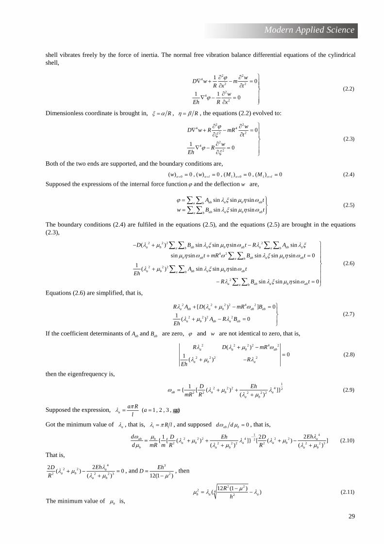
29


shell vibrates freely by the force of inertia. The normal free vibration balance differential equations of the cylindrical shell,

2 24

2 2

24

2

10

(2.2)1 1

0

wD w m

R x t

w

Eh R x

ϕ

ϕ

∂ ∂∇ + − = ∂ ∂ ∂ ∇ − = ∂ Dimensionless coordinate is brought in, Rξ α= , Rη β= , the equations (2.2) evolved to:

2 24 4

2 2

24

2

0

(2.3)1

0

wD w R mR

t

wR

Eh

ϕξ

ϕ ξ

∂ ∂∇ + − = ∂ ∂ ∂ ∇ − = ∂ Both of the two ends are supported, and the boundary conditions are,

0 1 0 1( ) 0 , ( ) 0 , ( ) 0 , ( ) 0 (2.4)l lw w M Mα α α α= = = == = = =

Supposed the expressions of the internal force functionϕ and the deflection w are,

sin sin sin(2.5)

sin sin sin

ab a b aba b

ab a b aba b

A t

w B t

ϕ λ ξ µ η ωλ ξ µ η ω

= = ∑ ∑∑ ∑

The boundary conditions (2.4) are fulfiled in the equations (2.5), and the equations (2.5) are brought in the equations(2.3),

2 2 2 2

4 2

2 2 2

2

( ) sin sin sin sin

sin sin sin sin sin 0(2.6)1

( ) sin sin sin

sin sin sin 0

a b ab a b ab a ab aa b a b

b ab ab a b aba b

a b ab a b aba b

a ab a b aba b

D B t R A

t mR B t

A tEh

R B t

λ µ λ ξ µ η ω λ λ ξµ η ω ω λ ξ µ η ω

λ µ λ ξ µ η ωλ λ ξ µ η ω

− + − + = + − =

∑ ∑ ∑ ∑∑ ∑

∑ ∑∑ ∑

Equations (2.6) are simplified, that is,

2 2 2 2 4 2

2 2 2 2

[ ( ) ] 0(2.7)1

( ) 0

a ab a b ab ab

a b ab a ab

R A D mR B

A R BEh

λ λ µ ωλ µ λ

+ + − = + − = If the coefficient determinants of abA and abB are zero, ϕ and w are not identical to zero, that is,

2 2 2 2 4 2

2 2 2 2

( )0 (2.8)1

( )

a a b ab

a b a

R D mR

REh

λ λ µ ωλ µ λ

+ −=+ −

then the eigenfrequency is,

12 2 2 4 2

2 2 2 2 2

1{ [ ( ) ]} (2.9)

( )ab a b aa b

D Eh

mR Rω λ µ λλ µ= + + +

Supposed the expression, ( 1 , 2 , 3 , )a

a Ra

l

πλ = = ggg

Got the minimum value of aλ , that is, 1 R lλ π= , and supposed 0ab bd dω µ = , that is,

1 42 2 2 4 2 22

2 2 2 2 2 2 2 3

21 2{ [ ( ) ]} [ ( ) ] (2.10)

( ) ( )ab b a

a b a a b

b a b a b

d EhD Eh D

d mR m R R

ω µ λλ µ λ λ µµ λ µ λ µ−= + + + −+ +

That is,

42 2

2 2 2 3

22( ) 0

( )a

a ba b

EhD

R

λλ µ λ µ+ − =+ , and3

212(1 )

EhD µ= − , then

2 22 4

2

12 (1 )( ) (2.11)b a a

R

h

µµ λ λ−= −The minimum value of bµ is,

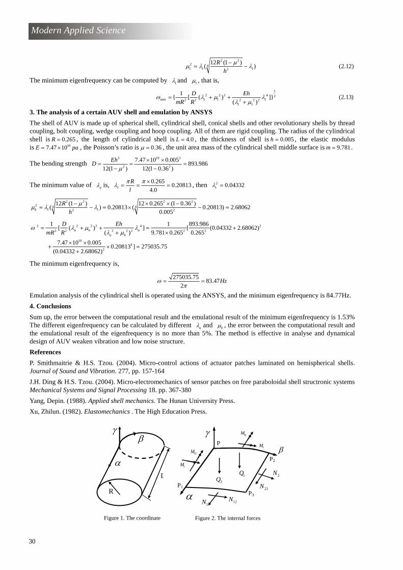
30


2 22 41 1 12

12 (1 )( ) (2.12)

R

h

µµ λ λ−= −

The minimum eigenfrequency can be computed by 1λ and 1µ , that is,

12 2 2 4 2

min 1 1 12 2 2 2 21 1

1{ [ ( ) ]} (2.13)

( )

D Eh

mR Rω λ µ λλ µ= + +

+

3. The analysis of a certain AUV shell and emulation by ANSYS

The shell of AUV is made up of spherical shell, cylindrical shell, conical shells and other revolutionary shells by threadcoupling, bolt coupling, wedge coupling and hoop coupling. All of them are rigid coupling. The radius of the cylindricalshell is 0.265R = , the length of cylindrical shell is 4.0L = , the thickness of shell is 0.005h = , the elastic modulus is 107.47 10E pa= × , the Poisson’s ratio is 0.36µ = , the unit area mass of the cylindrical shell middle surface is 9.781m = .

The bending strength 3 10 3

2 2

7.47 10 0.005893.986

12(1 ) 12(1 0.36 )

EhD µ

× ×= = =

− −

The minimum value of aλ is, 1

0.2650.20813

4.0

R

l

π πλ ×= = = , then 2

1 0.04332λ =

2 2 2 22 4 4

1 12 2

12 (1 ) 12 0.265 (1 0.36 )( ) 0.20813 ( 0.20813) 2.68062

0.005b

R

h

µµ λ λ− × × −= − = × − =

2 2 2 2 4 2

2 2 2 2 2 2 2

104

2

1 1 893.986[ ( ) ] [ (0.04332 2.68062)

( ) 9.781 0.265 0.265

7.47 10 0.0050.20813 ] 275035.75

(0.04332 2.68062)

a b a

a b

D Eh

mR Rω λ µ λλ µ= + + = +

+ ×

× ×+ × =

+

The minimum eigenfrequency is,

275035.7583.47

2Hzω π= =

Emulation analysis of the cylindrical shell is operated using the ANSYS, and the minimum eigenfrequency is 84.77Hz.

4. Conclusions

Sum up, the error between the computational result and the emulational result of the minimum eigenfrequency is 1.53%. The different eigenfrequency can be calculated by different aλ and bµ , the error between the computational result and the emulational result of the eigenfrequency is no more than 5%. The method is effective in analyse and dynamical design of AUV weaken vibration and low noise structure.

References

P. Smithmaitrie & H.S. Tzou. (2004). Micro-control actions of actuator patches laminated on hemispherical shells. Journal of Sound and Vibration. 277, pp. 157-164

J.H. Ding & H.S. Tzou. (2004). Micro-electromechanics of sensor patches on free paraboloidal shell structronic systems. Mechanical Systems and Signal Processing 18. pp. 367-380

Yang, Depin. (1988). Applied shell mechanics. The Hunan University Press.

Xu, Zhilun. (1982). Elastomechanics . The High Education Press.

P2

Figure 2. The internal forces

P1 P3

βP

α

γ

12N

1M

1Q2Q

Figure 1. The coordinate

L

R

α

βγ

1N

12M

2N

21N

1M

12M

31



Preparation and Performance Characteristics of

Resin-filled EVAL Hollow Fiber Membrane

Ling Chen

Key Lab of Hollow Fiber Membrane Materials & Membrane Process, Tianjin Polytechnic University

Tianjin 300160, China


Abstract

Take the ethylene-vinyl alcohol (EVAL) copolymer as the infrastructural material, the anion exchange resin D301R as the functional grains, adopt dry-wet method to make resin-filled EVAL hollow fiber membrane, test the pure water flux of the membrane, the rejection rate of the bovine serum albumin (BSA) and the static absorption performance of BSA. Check the influences of coagulation bath temperature and copolymer mass fraction to pure water flux and rejection rate. The experimental results indicate that the mass fraction of EVAL is 18%, the mass fraction of resin is 24%, and when the temperature of coagulation bath is in 40~50°C , the prepared resin-filled EVAL hollow fiber membrane has good mechanical intensity, high pure water flux, better BSA adsorption performance that the adsorption capacitance can achieve 25.04mgBSA/g membrane.

Keywords: EVAL, Hydrophilia, Ion exchange resin, Hollow fiber membrane

1. Introduction

As the hydrophilic membrane material, EVAL has its special advantages. EVAL is the crystal atactic polymer composed by hydrophilic vinyl alcohol unit and hydrophobic ethylene unit, which polymer chain has certain proportional hydroxide radical, so it has certain hydrophilia, and the experiment of contact angle (Matsuyama H, 2001, p.2583-2589& Young T H, 1998, p.717-724) also invalidates EVAL is the hydrophilic material, and this sort of material is not easy to be polluted when the albumens are separating, and CH2 unit endow it better mechanical intensity (T. Okaya, 1992), and it possesses good bio-compatibility and chemical stability, so it is fit for being infrastructural materials. As the filled grains, the ion exchange resin has certain adsorption capability to protein. This experiment takes EVAL as the infrastructural material, ion exchange resin as filled grains to spin hollow fiber membrane, and the prepared resin filled EVAL hollow fiber membrane albumen has large adsorption capacitance, combining the characteristics of large exterior area of hollow fiber membrane and hydrophilia of EVAL, which is not easy to be polluted.

M.E. Avramescu et al (M.E. Avramescu, 2003, No.218. p.219-233 & M.E. Avramescu, 2003, p.177-193 & M.E. Avramescu, 2002, p.155-173.) prepared resin-filled EVAL flat membrane adsorbent which had good adsorption capacitance and higher desorption rate for BSA, and changed the nature of the membrane for the affinity separation of protein. Zhang, Yuzhong et al adopted controlled phase separation method to prepare resin-filled EVAL fiber adsorbent which had good albumen adsorption capacitance and higher desorption rate, and formed coarse opening structure on the surface and with the increase of filling of resin, the coarseness degree and opening degree on the fiber surface was increased (Zhang, 2005, p.224-232).

This work takes EVAL as the infrastructural material, alkalescence anion exchange resin D301R as the functional grains, and adopts dry-wet method to prepare resin-filled EVAL hollow fiber membrane and described its performances.

2. Experiment

2.1 Raw materials

The infrastructural material is EVAL with 44% of ethylene content, and is made by Japan Kuraray Co., Ltd.

The filled grain is alkalescence anion exchange resin D301R made by Tianjin Nankai University Chemical Plant.

The solvent is DMSO made by Tianjin BODI Chemical Co., Ltd.

The additive is CP made by Tianjin Kermel Chemical Reagent Co., Ltd.

The model material is BSA made by China United Stars Industry Co., Ltd.

32


2.2 Experimental apparatus

(1) The spinning machine of chemical fiber made by Tianjin Motimo Membrane Eng. & Tech. Co., Ltd.

(2) The QUANTA 200 scanning electron microscope made by Holland FEI Company.

(3) The UV2450 ultraviolet and visible spectrophotometer made by SHIMADZU Company.

(4) HZQ-C air bath agitator made by Harbin Donglian Electronic & Technology Development Co., Ltd.

2.3 Preparation of resin-filled EVAL hollow fiber membrane

2.3.1 Preparation of micron-sized ion exchange resin

Because the granularity of the resin grain made by the factory is too large and the obtained filature liquid is not stable and easy to deposit and has only small adsorption capacitance, so we need to perform subsequent machining.

(1) Drying

The water content of the resin just out of the factory is higher, so we need to dry it and then crush it. Put the resin in the vacuum oven to dry it at 80°C until its weight doesn’t change.

(2) Crushing

We can adopt rubbing crushing method to obtain the micron-sized ion exchange resin.

2.3.2 Preparation of resin-filled EVAL hollow fiber membrane

To make resins evenly distribute in the filature liquid, with mixing around by the magnetic force, first put solvent, polymer and additive into three flasks, increase the temperature to about 60°C and continue to mix until dissolved, then put in resin several times and mix to stable filature liquid, and put in filature jar to be marinated for 24 hours. The prepared process to adopt dry-wet method to prepare resin-filled EVAL hollow fiber membrane is seen in Figure 1. The filature liquid is extruded from the tube spinneret, and the interior pore is filled with core liquid to make fiber form hollow. The thin flow of filature liquid directly enters into the coagulation bath through certain altitudinal air clearance and separation happens. The prepared fiber wipes off additive and solvent through bath, and is marinated in the 30% glycerite for 48 hours, and then is aired and stored.

2.4 Performance characteristics

2.4.1 Mensuration of pure water flux

We use the ultrafilter evaluation device made by Tianjin Motimo Membrane Eng. & Tech. Co., Ltd. to mensurate the pure water flux. Adjust the pressure to 0.1MPa, maintain the temperature at 25°C , and mensurate the membrane flux when the system is stable. Take the average through tests of several times, and compute the water flux according the following formula.

VQ

At=

Where, Q represents the water flux (L/m2.h), V represents the volume of the filtered liquid (L), A represents the effective area of the membrane (m2) and t represents the testing times (s).

2.4.2 Mensuration of rejection rate

Choose BSA which molecular weight is 67 thousands to dissolve in the cushion liquid which pH value is 7.4, confect 0.1% solution, maintain the solution temperature at the lower temperature, filtrate this solution by the prepared EVAL membrane small sample, take the original liquid and the corresponding filtered liquid, then measure the absorbencies of the original liquid and the filtered liquid by the UV2450 ultraviolet spectrometer. The computation formula of rejection ratio is

%100×−

=o

So

E

EER

.

Where, R represents the rejection ratio, Eo represents the absorbency of the original liquor and Es represents the absorbency of the sieved liquor.

2.4.3 Observation of membrane structure

We observe the membrane structure using QUANTA200 scanning electron microscope. Break the membrane in the liquid nitrogen, fix the sample in the clamp and dry it in the vacuum and at room temperature, then deposit a thin layer of gold on the surface in the vacuum, then we can observe the membranes section structure.

2.4.4 Static adsorption capacitance of protein

The protein static adsorption capacitance of resin-filled EVAL hollow fiber membrane can be confirmed by the BSA

interim adsorption experiment. The sorbent sample which we have know its quantity is marinated in the BSA cushion

33


solution until it balances (in this experiment, we adopt 24 hours), and we compute the static adsorption capacitance of resin-filled EVAL hollow fiber membrane to the protein through measuring the changes of BSA concentration. In the adsorptionexperiment, the pH values of the cushion solution we use are 7.4 and 9.1, and the material liquid protein BSA concentrationis 1mg/ml. The protein static adsorption capacitance of resin-filled EVAL hollow fiber membrane (Q) can be computed by thisformula.

Q = (C0 - C) V / W

Where, Q represents protein static adsorption capacitance (mgBSA/g membrane), C0 represents the initial concentration of

material liquid protein BSA (mg/ml), C represents the concentration when the material liquid protein BSA has implementedadsorption for 24 hours (mg/ml), V represents the volume of the material liquid (ml), and W represents the weight of themembrane sample (g).

3. Results and discussions

3.1 Structure analysis of resin-filled EVAL hollow fiber membrane

Figure 2 is the SEM photo of the resin-filled EVAL hollow fiber membrane structure. From the exterior in Figure 2, we can seethat there are micropore-structures in the exterior which can make BSA contact with resin through micropore. From thesection in Figure 2, we can see the resin enwrapped by the polymer, and when the BSA material liquid fills EVAL hollow fibermembrane through resin, it contacts the resin and achieves the function of adsorption. From the interior in Figure 2, we cansee many protuberances, because in the membrane forming process, due to high speed separation, resins are assembled tothe interior in the exchange process of solution and water, many protuberances and stains are formed.

3.2 Influence of coagulation bath temperature to the performance of resin-filled EVAL hollow fiber membrane

Fix the mass fractions of resin and the EVAL, control the temperature of coagulation bate is in 20~60°C , we will check theinfluences of coagulation bath temperature to the pure water flux and rejection rate.

The temperature of coagulation bath is an important factor to influence the membrane structure and performance. FromFigure 3, we can see that with the gradual increase of coagulation bath temperature, the pure water flux of resin-filled EVALhollow fiber membrane gradually increases, and the rejection rate gradually reduces. After the thin flow of filature enters intothe coagulation bath, the solvent in the casting membrane liquid begins transferring to the coagulation bath, which makesthe concentration of the polymer in the casting membrane liquid gradually increase, and polymers begins to assemble eachother, so the membrane is finally formed (Gao, 1989). When the temperature of coagulation bath increases, the exchangespeed between solvent and nonsolvent quickens and first the compact layer rapidly forms, and coagulation bath quicklyimmerges in the interior of the membrane, and the mixing speed of the dense and rare phases in the membrane interiorbecomes quick, which makes the membrane interior form more big cavums, accordingly make water flux continually increaseand the rejection rate gradually reduce. Too high or low temperature of coagulation bath temperature is not propitious to themolding of the membrane, and when the temperature is too high, the exchange speed of solvent and nonsolvent is quick andthe membrane is easy to induce stains, and when the temperature is too low, the formed membrane is dense, which inducesthe flux is very low. This experiment selects the temperature of 40~50°C as the best coagulation bath temperature.

3.3 Influence of EVAL mass fraction to the performance of resin-filled EVAL hollow fiber membrane

Take DMSO and CP respectively as the solvent and the additive, fix the mass fraction of the resin D301R in 16%, increasethe mass fraction of EVAL to 13%~19%, we will check the influences of EVAL mass fraction to the pure water flux andrejection rate.

As seen in Figure 4, when the concentration of EVAL increases from 13% to 19%, the pure water flux of resin-filled EVALhollow fiber membrane will reduce with it and the rejection rate will increase with it. When the mass fraction of EVAL is in13%~19%, with the increase of EVAL mass fraction, the performance of forming membrane gradually becomes better. Withthe increase of polymer concentration in the filature liquid, the voluble degree among macromolecule chains increases, butthe polymer poor phases which can form membrane exterior pores and channels relatively reduce, so with the increase ofpolymer concentration, the pure water flux of the membrane reduces and the rejection rate increases. But when the contentof high polymer EVAL is lower, the agglutinate degree of the filature liquid is lower, which makes the spun hollow fiberconfiguration is difficult to be controlled and has lower intensity. Therefore, synthetically considering two factors includingpure water flux and hollow fiber membrane intensity, this experiment take the best concentration 18% as the emphasis tostudy.

3.4 Influence of resin mass fraction to the performance of resin-filled EVAL hollow fiber membrane

3.4.1 Influence to BSA rejection rate

When the pH value of BSA solution is 7.4, the rejection performance of resin-filled EVAL hollow fiber membrane is best, sowe only study the rejection rate of the membrane when the pH value is 7.4.

Table 1 shows the rejection data of the resin-filled EVAL hollow fiber membrane with different resin-filled quantities. Asviewed from the data, when the mass fraction of the polymer is fixed, with the increase of resin mass fraction, the rejection

34


rate of hollow fiber membrane increases, the resin content increases, the adsorption ability to the albumen also increases,the albumen concentration in filtered liquid reduces, the rejection rate increases. But as viewed from the integration, therejection rate is very low, and when pH value is 7.4, the fiber mainly depends on the aperture to reject the BSA molecules,which causes maybe is that the aperture of the hollow fiber membrane is too big, or the membrane has stains, which willinduce lower rejection rate.

3.4.2 Influence to BSA static adsorption capacitance

One important function of the resin mass fraction to resin-filled EVAL hollow fiber membrane is that it fair influences theadsorption capacitance of the protein. This experiment chooses the cushion liquids which pH value are respectively 7.4 and9.1.

Fix the 18% of mass fraction of EVAL polymer, increase the mass fraction of resin D301R, from Figure 6 we can see that withthe increase of resin mass fraction, the adsorption capacitance of BSA will increase. When filling the resin grains to themembrane, because of the increase of adsorption function radicel in the membrane radicel, the static adsorption capacitanceof membrane to BSA will be enhanced. Combining Figure 5, we can see that with the increase of resin mass fraction, theadsorption spots will increase, and the adsorption capacitance to BSA will also increase.

3.4.3 Influence to structure

From Figure 7, we can see that with the increase of resin mass fraction, the resin grains obviously increase on the section ofresin-filled EVAL hollow fiber membrane, and exterior and interior gradually become uneven because of the resin grainsexisted in the high polymer. When the resin content is lower, the resin grains in EVAL present single individuals which aredistributed evenly and enclosed by polymers and in the forming process of the membrane, the high polymers beginseparation, the disturbed function of the resin grains is not obvious, and when the resin content further increases, thedisturbed function of the resin grains increase, and the stains on the interior of the hollow fiber membrane also increase withit. When the resin content is low, the high polymer EVAL in the resin-filled EVAL hollow fiber membrane has less structuredeficiencies. With the increase of resin content, though the distribution of the solid grains inclines to even, but the wholestructure inclines to loosening, and the deficiencies such as the microcracks and hollow pores become more.

4. Conclusions

(1) This experiment adopts the dry-wet method to prepare resin-filled EVAL hollow fiber membrane, and the prepared hollowfiber membrane has higher pure water flux and good BSA static adsorption capacitance.

(2) The pure water flux increases with the increase of coagulation bath temperature and reduces with the increase of EVALcontent of the polymer, and when the temperature of the coagulation bath is in 40~50°C and the mass fraction of the polymeris 18%, the every sort of performance of the resin-filled EVAL hollow fiber membrane is excellent.

(3) With the increase of mass fraction of the ion exchange resin, the static adsorption capacitance of BSA increases, andwhen the resin mass fraction is 24% the adsorption performance and mechanical intensity are good.

References

Gao, Yixuan & Ye, Ling. (1989). Membrane Separation Technology Base (First Edition). Beijing: China Science & Technol-ogy Press. March 1989.

Matsuyama H, Kobayashi K, Maki T, et al. (2001). Effect of the ethylene content of poly (ethylene-co-vinyl alcohol) on theformation of microporous membranes via thermally induced phase separation. Journal of App Polym Sci. No.82. p.2583-2589.

M.E. Avramescu, M. Wesslling, et al. (2003). Preparation of mixed matrix adsorber membranes for protein recovery. Journalof Membrane Science. No.218. p.219-233.

M.E. Avramescu, W.F.C. Sager and M. Wesslling. (2003). Functionalised ethylene vinyl alcohol copolymer (EVAL) mem-branes for affinity protein separation. Journal of Membrane Science. No.216. p.177-193.

M.E. Avramescu, W.F.C. Sager, M.H.V. Mulder & M. Wesslling. (2002). Preparation of ethylene vinyl alcohol copolymermembranes suitable for ligand coupling in affinity separation. Journal of Membrane Science. No.210. p.155-173.

T. Okaya, K. Ikari, in: C.A. Finch (Ed.). (1992). Polyvinyl Alcohol Developments. Wiley, New York. (Chapter 8).

Young T H, Yao C H, Sun J S, et al. (1998). The effect of morphology variety of EVAL membranes on the behavior ofmyoblasts in virtro. Journal of Biomaterials. No.19(7-9). p.717-724.

Zhang, Yuzhong & Li, Ran. (2005). Preparation of resin filled EVAL fibrous adsorbents and characteristics of their adsorption.Ion Exchange and Adsorption. No.21(3). p.224-232.

35


Figure 1. Preparation Equipment of Resin-filled EVAL Hollow Fiber Membrane by Dry-wet Method

Spinning solution

Spinneret

Coagulation bath (H2O)

External liquid

Figure 2. SEM Photo of Resin-filled EVAL Hollow Fiber Membrane Configuration

Resin

Exterior Interior Section

20 30 40 50 600

1000

2000

3000

4000

Temperature of coagulation bath (℃℃℃℃)

Flu

x of

pur

e w

ater(

L/m

2 .h)

0

20

40

60

80

100

Rej

ectio

n of

BS

A (

%)

Figure 3. Influence of Coagulation Bath to Pure Water Flux and BSA Rejection Rate

36


12 14 16 18 20

900

1200

1500

1800

EVAL concentration (%)

Flu

x of

pur

e w

ate

r (L/

m2 .h

)

54

57

60

63

Re

ject

ion

of

BS

A (

%)

Figure 4. Influence of EVAL Mass Fraction to Pure Water Flux and BSA Rejection Rate

8 12 16 20 24

5

10

15

20

25

Sta

tic a

dsor

ptio

n ca

paci

ty o

f BS

A(

mg/

g)

Concentration of resin(%)

pH=7.4 pH=9.1

Figure 6. Influence of Resin Mass Fraction to BSA Static Adsorption Capacitance

Resin content 10% Resin content 15% Resin content 24%

Figure 5. Section SEM Photo of Resin-filled EVAL Hollow Fiber Membrane with Different Mass Fractions

37


Exterior Section Interior

A1 A2 A3

B1 B2 B3

C1 C2 C3

Figure 7. SEM Photo of Resin-filled EVAL Hollow Fiber Membrane with Different Mass Fractions

(Mass fraction of EVAL is 18%. In A1 ~ A3, the mass fraction of resin is 10%. In B1 ~ B3, the mass

fraction of resin is 18%. In C1 ~ C3, the mass fraction of resin is 24%.)

Table 1. Rejection performance of resin-filled EVAL hollow fiber membrane with different resin mass fractions

D301R/EVAL 10/18 12/18 15/18 18/18 21/18

Rejection Rate (%) 5.6 13 18 43 55


38

Vol. 2, No. 1


Research of Quality Improvement and Quality

Innovation Based on Knowledge Fermenting Model

Jin Wang, Jinsheng He, Jiansheng Tang

School of Management, Tianjin University, Tianjin 300072, China

Abstract

Quality improvement and quality innovation are the important approach to enhance competitive force for enterprises.Quality improvement is a process of knowledge innovation in nature which must be actualized by organizational learning.This article starts from the relations among quality improvement, quality innovation and the ability of organizationallearning, analyzes the knowledge moving rule in the interior process of quality improvement and innovation and expatiateson the creation, development and diffusion mechanisms of quality knowledge in the quality flow based on the knowledgefermenting theory of organizational learning. Furthermore, taking the quality control (QC) group as an example, this articleanalyzes the behaviors and functions of nuclear factors such as quality knowledge sourdough, quality knowledge matrixand quality knowledge enzyme in the process of quality knowledge fermenting, and these nuclear factors function mutuallyin the quality knowledge fermenting bar. This article also puts forward five types of quality knowledge fermentation andanalyzes their characters respectively, points out the implementation of knowledge fermentation possesses meanings toenhance the level of quality improvement and quality innovation for enterprises.

Keywords: Quality innovation, Quality improvement, Knowledge fermenting, Organizational learning

1. Introduction

With the globalization of economy, quality information increases explosively and quality innovation emerges in endlessly.More innovations in modern large-size enterprises are from the intersection and integration of multiple knowledge andmutual endeavors of organizational members, which can not be provided by individual’s ability, but needs the innovativeabilities of organization ore colony, i.e. the ability of organizational learning. As viewed from this meaning, the qualityimprovement and quality innovation of enterprise are the process of knowledge innovation in essential. The ability ofknowledge innovation is decided by the organizational learning ability, so to realize continual quality improvement andinnovation of enterprises through organizational learning has become the important task in the domain of quality manage-ment and knowledge management.

Under this background, in this article we analyze the knowledge attributes in the process of quality improvement and qualityinnovation and study the mechanism of creation, development and diffusion of quality knowledge in the quality flow.Taking QC group as an example, we also research the types (including assimilation fermentation, adaptive fermentation,encounter fermentation, evolution fermentation and reforger fermentation) and characters of quality knowledge fermenta-tion and point out the meanings of the implementation of knowledge fermentation for enhancing the level of enterprisequality improvement and quality innovation.

2. Relations among quality improvement, quality innovation and organizational learning

In fact, for the relation of quality and organizational learning, quality management master Deming had sparkplugged that itis a learning cycle through changing the step “check” in the cycle of PDCA (plan, do, check, act) put forward by him to“study” as early as in 1986. Another quality expert Juran emphasized that “TQM is a sort of learning movement which makespeople want to study and development”. Japanese quality master Ishikawa put forward the usage of quality cycle in theprocess of improving performance. The base of quality cycle is based on the following principles: unconstraint, selfdevelopment, everyone participation, mutual development and durative. To work together for the team must base on thefreewill sharing of durative latent knowledge. Ron Dvir analyzed the futures of quality management team and knowledgemanagement, made these two aspects to affiliate, and proved that both sides had mutual stimulative relation from demon-stration and reasoning again.

Quality management is correlative with knowledge management and organizational learning, which can be seen from thedefinitions of organizational learning and quality management. The organizational learning is defined as the process ofenhancing improvement through better cognitions, which is very similar with the target and process of quality improvement.Another definition of organizational learning is the process of checkout and correction. Though these relations exist

39


between organizational learning and quality management, but there are few researches for the integration of them. Maric C.,Ferguson Amores et al put forward the hypothesis that complete quality management and learning organization not onlycan not be dissevered, but also can complemented each other, compared both characters through literature summarizationand case analysis, and validated in which aspects they can complemented each other. QC group is an important organiza-tional conformation in quality management, some scholars has realized the importance of organizational learning in QCgroup. Qu, Kunru pointed out the creation and development of QC group was a process syncretizing western and easterncultures and continually implementing quality management and knowledge innovation, and to follow this process self-consciously must promote the knowledge innovation of enterprise. Liuyu used MIT professor Peter M. Senge’s fivestrategies to discuss establishing innovative QC group and making it possess the ability keeping innovation from fiveaspects such as fostering innovative character, activating innovative motivation, building innovative team, inspiring cre-ativity of colony and training innovative thinking. Long, Yuzhen pointed out that the establishment of learning team canfully promote the sustainable developments of QC group, and discussed how learning organization utilizes the sustainableinnovation, high efficient operation and efficient communication of QC group from the characters of learning team. Withregard to learning methods, Liu, Zhaoyan deeply analyzed the application of learning organization in quality managementfrom two aspects including “single-loop learning, double-loop learning” and “study how to study, study map” on the 1st

Proseminar of Learning Organizational theory leading and Application Tendency.

From above researches, we can see that foreign and domestic academe and enterprise industry have begun to attemptaffiliating quality management with organizational learning. However the results are limited. Though they emphasized theimportant functions of organizational learning in quality management, but there are few systematic researches how relativetheories of organizational learning improve the development of quality management. The domain of quality managementhas not definitely and self-consciously adopted the theory view of organizational learning to study quality management,which is first embodied in that the present popular quality standard system has not taken organizational learning as thegolden rules and method of quality management, and in practice large numbers of quality operators also lack the concept oforganizational learning. Under this situation, the principle of organizational management contained in the standard andframe of quality management can not be easily and truly understood and implemented.

To explain the mechanism of the creation, development and diffusion of quality knowledge in quality flow by means ofintroducing knowledge fermenting model also offers clear approach for quality improvement and quality innovation.

3. Knowledge fermenting model of organizational learning

(1) The development of organizational knowledge is always from a sort of “initial knowledge” which is also called knowl-edge sourdough.

(2) The development of knowledge depends on “knowledge matrix” with definite quality. The knowledge matrix includesthree aspects. The first one is active (reactive) knowledge, i.e. people who participate in the process of the research fromknowledge innovation to knowledge fermentation. They can continually complement knowledge “nutrient” to initial knowl-edge through mutual communication. The second one is the passive knowledge which includes knowledge and informationsuch as file, data and audio-video data obtained from various channels. This knowledge needs be selected and exerted bypeople, and it also can offer knowledge “nutrient” for knowledge fermentation. The third one is the knowledge enzyme,which can assimilate knowledge boundaries, promote knowledge integration, evolvement and communication.

(3) The knowledge fermenting bar is a place which can implement knowledge “colony affinity”. In knowledge fermentingbar, under the “nourishing” of knowledge matrix and materials of knowledge and information, the initial knowledge canobtain developments and multiplying through the catalysis of knowledge enzyme.

(4) The environment means rich and colorful objective phenomena and things. It can offer various resources of knowledge,information and intelligence including various contradictions people face and practical checkup standards of knowledge.The intelligence resource and knowledge information resources are obtained from environment.

(5) Knowledge and information tools (such as IT and communication technology) help people to acquire various knowledgein initial knowledge and knowledge matrix.

(6) The results of knowledge fermentation are continual increase of organizational knowledge. The level of knowledgeenvironment and knowledge technology will influence the efficiency and effects of knowledge fermentation.

4. Analysis of quality improvement and quality innovation based on knowledge fermenting model

From the knowledge fermenting model, we can see that the knowledge fermentation mainly emphasizes several factorsinfluencing knowledge increase such as “knowledge sourdough”, “knowledge matrix”, “knowledge enzyme in knowledgematrix” and “knowledge fermenting bar”. Taking QC group as an example, we will expatiate on the functions of QC group inorganizational learning.

4.1 Quality knowledge sourdough

How enterprises put forward exact requirement of quality improvement and quality innovation is the start that qualityimprovement and quality innovation can be created, and the process to find out this requirement can be called the processto find out knowledge sourdough. To timely and efficiently find this quality knowledge sourdough is the sign whether QC

40


group possesses thinking energy. Traditional QC group usually has fixed members who apply themselves to find problemsin work and solve them together. If QC group can not systemically try to find new quality originalities and quality targets,it will induce disappearance of new ideas and new thinking methods, and finally go to deathly stillness. Therefore, in thedevelopmental process, QC group should solve the problem of the origin and creation of “quality knowledge sourdough”,which include continual update of knowledge body, mechanism that new people participate and opening work methods.There are several channels can help QC group obtain quality knowledge sourdough.

(1) Problem sourdough. It means the problems occurring in the movement of organizational quality management.

(2) Standard sourdough. It means the quality management methods in excellent organizations.

(3) Exterior brain sourdough. It means the diagnoses that quality experts or exterior quality auditor made to organizationalquality management.

(4) Inspiration sourdough. It means new ideas and new originalities in the movement of organizational quality management.

These quality knowledge sourdoughs are not produced without foundations, which are closely relative with organizationalmovements. The evocators of quality knowledge sourdough mainly include organizing routine quality movements, thequality movement evocated by special problems and the quality movement taking development as its aim. To organizeroutine quality movement means the originalities produced because of factors such as organizing quality managementsystem, working habits, and seasonal knowledge convening process, such as seasonal quality group movement, qualitymeeting and so on. The quality movement evocated by special problems is that the organization adopts actions to solvecertain quality problems, for example, the organization solves the quality problem produced by consumer’s opinions. Thequality movement taking development as its aim is that the organization implements quality movement in order to furtherenhance quality, such as pursuing 6ó, realizing zero deficiency and so on. Except for above evocators, all supplier, consumer,competitor, cooperator of the organization are the indirect factors to evocate quality knowledge sourdough. The organiza-tion should establish proper quality development strategy to create better environment for the creation of quality knowl-edge sourdough.

4.2 Identification and improvement of quality knowledge matrix

Aiming at the tasks or requirements of quality improvement, how can QC group realize the object of quality innovation?Obviously, random constituent QC group unnecessarily possesses the innovative ability. The buildup of QC group is thekey of quality innovation. The concept of knowledge body is to put forward a sort of specific guideline and require groupmembers’ knowledge composing and learning ability can fulfill the requirements to capture quality difficulty. In the processof solving problems, traditional QC group doesn’t consider whether group members possess the ability to solving problems,which restricts the functions of QC group. Therefore, QC group can improve the matrix of quality knowledge through manymethods such as training, expert guidance and opening composing mechanism.

The matrix of quality knowledge includes active quality knowledge matrix, passive quality knowledge matrix and qualityknowledge enzyme (because of the importance of quality knowledge enzyme, we will discuses it alone). The active qualityknowledge matrix mainly means experts, scholars and personnel with quality knowledge in the organization, and theyactively participate in quality improvement and quality innovation, communicate each other and continually complementand perfect initial knowledge by means of their own quality knowledge. The passive quality knowledge matrix mainly meansthe technical materials and experiment facilities about quality management in the organization. Quality knowledge matrix isthe main body of quality knowledge fermentation which can directly influence the effects of quality knowledge fermentation.Therefore, the organization should try to improve quality knowledge matrix, and enhance efficiency and effects of qualityknowledge fermentation. The improvement of active quality knowledge matrix can adopt many methods such as qualitytraining, quality knowledge communication, talk and discussion, quality management consultation, and the introduction ofquality talents. The improvement of passive quality knowledge matrix can be actualized by establishing quality knowledgerepository.

4.3 Quality knowledge enzyme

Though having experts with different professional knowledge backgrounds and from different departments, but how tocooperate is another key to complete quality innovation aim for QC group. As learning QC group, it must need flat organi-zational structure which can be full of democratic spirits, fully mobilize everyone’s enthusiasm, so we can consider devel-oping people with authority, ability, objectivity and backgrounds of management and psychology as the cadreman oforganizational learning who can exert functions of elicitation, inducement and promoting to realize quality innovation. Frompast abortive lessons of QC group, some enterprises only externally studied other successful QC group, and they didn’tmobilize QC members’ enthusiasm and creativity, so QC group was only stay on the form.

In organizational learning, the factor which has functions of organization, agency, harmony, communication and promotingis called knowledge enzyme. To promote quality knowledge fermentation, the organization should especially emphasize thecooperation and catalysis of quality managers, because the quality managers are the constitutor and executor of qualitysystem and quality culture, the organizer of organizational quality movement and they can connect quality knowledge andtheir carriers in different spaces and different sorts, so the quality managers are the main form of quality learning (knowledge)

41


enzyme who have functions of agency and bridge. Outstanding quality managers in enterprise are the key to acquiresuccesses for quality innovation. When many enterprises implement standards such as ISO9000 or HSE, they usually adoptoutsourcing to solve the establishment problem of quality system, which is the classic example to enhance quality levelthrough enhancing learning enzyme. The quality managers of the organization should realize their core function in cata-lyzing quality improvement and quality innovation, and promote quality innovation of enterprise through enhancing theirown “livingness”. Their functions include layout of quality strategy (long term layout, middle term layout, short termlayout), organizing movements of quality knowledge value chain (quality knowledge acquiring, quality knowledge sharing,quality knowledge innovation, quality knowledge protection, quality knowledge application), establishing quality systemand rules and supervising implementation, proper promoting (promoting rules, locale promoting), evaluation andimprovement, and quality culture construction (such as cultures making for quality knowledge sharing and innovation).

4.4 Quality knowledge fermenting bar

The quality knowledge fermenting bar means the place or mechanism that various factors in or out organization are gatheredto implement “colony affinity” of quality knowledge. Except for personnel and knowledge, out of question, QC group alsoneeds the support of material conditions such as flat organizational structure making for communication, base establish-ment and environment convenient for team communication, democratic decision-making mechanism, resource distribution,leaders’ support and emphasis. The gathering of these resources offers the place and opportunity to communicate forgroup members. Under different conditions, knowledge fermenting members have different aims and gatherings and formdifferent fermenting forms.

(1) Assimilation fermentation. In the process when QC group extends experience and knowledge, the knowledge receiversneed combine exterior experiences with their original knowledge and experience, chaw and understand knowledge andachieve right operation to knowledge, which is assimilation fermentation. The introduction of learning organization andlarge numbers of relative researches fully indicate the important function of assimilation fermentation.

(2) Adaptive fermentation. QC group cannot simply and mechanically apply quality management experiences of otherenterprises. It must establish an implementation standard combining the principle of quality management system and thepractice of enterprise to realize the increase function of ISO9000 for enterprise. When knowledge is used in practice and theapplication object of knowledge changes, the adaptive evolvements are usually needed and take effect, which indicates theknowledge fermenting function has high adaptability.

(3) Encounter fermentation. QC group centralizes experts’ (supplier and consumer) knowledge of many subjects in theinterior or exterior of enterprise to dig tackling tasks or problems faced by enterprise and produce new plan, new method andnew knowledge, which is encounter fermentation. The encounter fermentation includes assimilation fermentation andadaptive fermentation.

(4) Evolvement fermentation. Just as sourdoughs will selecting the superior and eliminating the inferior with the change ofenvironment, knowledge is evolving continually, and people can not isolate us on the experiences, technology and meth-ods that we have already had for ever. If the implementation of ISO9000 is a sort of adaptive fermentation, so the update ofISO9000 such as from edition 94 to edition 2000 is a sort of process of evolvement fermentation.

(5) Reforger fermentation. The fermenting process can produce bran-new species and matters. Some essential innovationsof QC group are also a sort of result of knowledge fermentation, for example, the introduction of ISO9000 belongs toinnovative fermentation, though before it is introduced, the practice and theory researches has acquired quiet great devel-opments about the establishment of quality system, but as a sort of new management technology and authenticationsystem, its establishment realizes qualitative flight.

Table 1 is the character comparison of traditional QC group and the QC group with organizational learning, and it embodiesthe function of organizational learning to QC group. From analysis in the table we can see that the QC group after organiza-tional learning has stronger innovative ability and is fitter for the competition with rapid changes.

5. Conclusions

Starting from the development rule of quality management, in this article we demonstrate the theory that the furtherdevelopment of quality management needs deep research of organizational learning. Based on past researches on therelation of quality management and organizational learning, we point out these researches were still staying on the stageemphasizing the importance of organizational learning to quality management. This article introduces the convening-fermenting model of organizational learning into quality management, takes QC group as an example, detailedly analyzes theexistence forms of quality knowledge sourdough, quality knowledge matrix, quality knowledge enzyme and quality knowl-edge fermenting bar and their function mechanism to quality management, compares the character differences betweentraditional QC group and the QC group with organizational learning, offers references for further development of qualitymanagement.

References

Alira Srdoc, Alojzij Sluga & Ivan Bratko. (2005). A Quality Management Model Based on the “Deep Quality Concept”.International Journal of Quality & Reliability Management. No.22(3).

42


Elena Bou & Alfonso Sauquet. (2004). Reflecting on Quality Practices through Knowledge Management Theory: Uncover-ing Grey Zones and New Possibilities of Process Manuals, Flowcharts and Procedures. Knowledge Management Research& Practice. No.2.

Liu, Zhaoyan. (2004). Application of Learning Organization in Quality Management. 1st Proseminar of Learning Organiza-tional theory leading and Application Tendency. Beijing.

Qu, Kunru. (2001). Three Distensions of Knowledge Economy and Roles of QC Groups. Journal of Xi’an Shiyou University(Social Sciences). No.10(1).

Zhang, Gongxu. (2004). Century Quality Management Course and Present Quality Management Situation. Quality andReliability. No.3.

System Subsystem Traditional QC group QC group with organizational learning

Time Existent time Middle/ Long term Long term Aim Problem oriented Ability oriented

Value view Development of enterprise Mutual development of personnel and enterprise Culture

Will Quality oriented Extensive, not only limited in quality domain

Sourdough Source Mainly inner Introducing new exterior ideas often

Maturity uncertainty Maturity Knowledge matrix Knowledge needed

Professional quality knowledge

Comprehensive knowledge

Action mode authoritative Cooperative and communicational

Knowledge enzyme Mode of

organizational cooperation

Organic, professional Organic, incompact (based on mutual trust)

Boundary Yes No Learning method Single-loop learning Double-loop learning Knowledge

bar Layer

Static, more efficient on the operation layer

Dynamic, more efficient on the strategic and tactic layers

Ability Quality guarantee ability

High High

Table 1. Characteristic comparison between traditional QC group and QC group with organizational learning

Figure 1. Knowledge Fermenting Model

Sourdough

Knowledge Matrix

Organizational Cooperation

Knowledge

Technology

Knowledge Source

Knowledge Fermenting Bar

Technology Source

Knowledge Environment Updating

Knowledge

43



Mobile Government: New Model for E-government in China

Peiyu Wang

E-Commerce, Information Management School, Wuhan University, Wuhan 430032, China


Abstract

This article examines the feasibility of spreading “e” of e-government from solely web-based technology to mobile fieldafter reviewing the development of e-government in China and the present situation of China. Through comparing withtraditional web-based e-government and analyzing experiences in both western country and China, a new model GMCC(Government Management & Call Center) is put forward as an assistant construction of m-government.

Keywords: M-government, E-government, GMCC, China

1. Introduction

There is not any universally accepted definition of the e-government concept (Halchin, 2004, pp. 406-419., p. 407), thusthere are different comprehension of electronic. In the definition of e-government by Means, “e” refers to “electronicmeans” ( Means and Schneider. 2000, pp.121); In UN & ASPA, 2002, “e” was defined as “Internet and the World-Wide-Web”(2002); and P.T. Jaeger took it as including using other ICTs in addition to the Internet and the Web, such asdatabase, networking, discussion support, multimedia, automation, tracking and tracing, and personal identification tech-nologies (Jaeger, 2003, pp.323-331). In this article, we intentionally take electronic of e-government in a broader way as theintegration of Internet, telephones, and call centers.

E-government since its debut has evolved four stages in China (He & Yang,2006,pp.37):

Initial stage: Office Automation Project (OA). Central and regional governments started to apply OA in mid 80s, 20thcentury. Government agencies began to use computers for office work and few information centers were establishedduring this period.

Application stage: Informationization of Government Affairs. This period started from the 1990s when the “Tri-GoldenProject”-abbreviation for the Golden Bridge, Golden Gateway and Golden Card project-was first sketched to be carried outby the central government aiming at a systematic informationization of government affairs. The main points are laid oninfrastructure construction for informationzation and for data and other information exchange for strategically departments.

Developing stage: Government Connection Project(GCP). E-government in late 1990s entered its time of prosperity due tocontinuous development of net-building technologies and information infrastructure. Early in the year 1998, the firstnetwork for information sharing was established in Shenzhen (Liu, Xu and Nie, 2005). In 1999 information centers in morethan 40 ministries (departments, agencies) advanced a proposal of the establishment of the “Government ConnectionProject”, which paved the way for further development of e-government.

E-government in China is now in the forth stage which could be termed as e-government Project. The passage of “e-government Construction Guidelines in China” on July.3rd by National Informationzation Group is a milestone whichsignals a new step for balanced overall planning and progress of e-government in China.

As Mobile telecommunication tools have always been featuring their affordable prices with strong capabilities of interac-tion and a user specific service system which all come down to one point of creating a user friendly interface, it’s of highlypossible for a publication of electronic government administration oriented towards the public on the premise of a well-defined information system from the aspect of mobile telecommunication.

2. Construction of m-government

2.1 basis of m-government realization

Considering the present situation of China, there are two primary factors that make m-government application feasible:

2.1.1 Popularization of mobile phones

Until the time of Dec. 2006, there are up to 137 million netizens and more than 450 million people are enjoying the benefitsof Mobil phones nationwide, which is about 3.2846 times the number of the internet users in this country (2007). In other

44


reports, 93% city dwellers and an average of 33.9% of the whole population are entitled to cell phone services(Song, 2006),among whom 17 million access to the Internet through handset and are accounting for a roughly 12.4 percent ofwholeneitizens (2007). From these statistics, we could see the popularization of mobile infrastructure in China and diversitycurrent of Internet access based on combination of non-stationary and Internet-based terminals.

2.1.2 Maturity of mobile telecommunication technology

The amalgamation of mobile telecommunication and mobile computing accelerate the development of mobile technology.Mobile interaction resulting from the application and development of mobile technology makes Ubiquitous Computingand Anytime & Anywhere connection no more a theory and meanwhile provides a solution for real-time informationexchange.

There are mainly 4 types of mobile technologies (Song, 2006):

(1)Radio-based two-way telecommunication (for exclusive or public use) and broadcasting.

(2) Mobile phonic service based on beehive phone, Short Message Service (SMS), Multi-media Messaging Service(MMS) and the Wireless Application Protocol (WAP), General Packet Radio Service(GPRS) and the 3rd Generation(3G).

(3)Services on the availability of mobile apparatus, including laptop, Personal Digital Assistant (PDA), beeper, RadioFrequency Identification(RFID) and Global Positioning System(GPS).

(4) Wireless network like WIFI, WIMAX, blueteeth, etc.

2.2 Contents of m-government

2.2.1 Services based on message

Short message is the representative. It resembles e-mail on Internet, which acquires low technology while realizes broadestapplication. Most e-government digital services sprouted on early stage belong to this category, such as message bulletin(water pollution report in Harbin); inward short message (meeting announcement by sending messages in Guang Donggovernment department); outward short message (feedbacks to customs of its transaction application) (April 4, 2007).Information flowing direction of services based on message transferring could be either unidirectional or di-directional.Government can send messages to all mobile users in an area without knowing exact numbers and mobile users can acquireor customize information by sending message without entangling in complex government organization.

2.2.2 Services based on Anywhere Internet Access (AIA)

Anywhere Internet Access (AIA) means the combined application of GPRS, CDMA and the future 3G data transferringtechnology (Song & Li, 2006). Some typical examples are the city supervising system in Beijing and other regional systemsof police resource management. AIA technology is also useful on occasions of distant data acquirements in environmentprotection departments, security agencies and dangerous material surveillance department. And WAP, this type of publicservice should be included since netizens are also given access to government information via GPRS, CDMA whichembodies the same function of other e-government applications. These WAP sites have been built by the Hong KongSpecial Administrative Region Government and some mainland governing structures.

2.2.3 Interactive voice response system (IVRS)

Interactive Voice Response Systems (IVRS) are extensively used for common and structured transactions such as informa-tion about ticket reservation, knowing the bank balance, authorizing a transaction, knowing the position of an applicationor complaint, and authentication of user for secured transactions (Awdhesh and Rajendra, 2007). For example, the IndianRailways provide instant information regarding the confirmation of the tickets, positions of the train by its IVRS (April 4,2007)query system.

2.3 Government assistant: Government Management & Call Center

In July 2005, Song Gang brought forward “setting up two centers”. The one is Supervision Center, which is an indepen-dent entity with recruited mobile supervisors and operate a call center as well. The other is Command Center. whosefunction of coordination is reinforced based in District Integrated Municipal Administration Commission. Responsibilityof Mobile Supervisors are as follows: Report to and receive orders from the supervision center; Responsible to inspectand confirm problems in relevant cells; Constant connection to the supervision center through the mobile handset;Position and working status monitored by the supervision center (Song, 2005).

Awdhesh K.Singh and Rajendra Sahu established GCC model (Awdhesh and Rajendra, 2007). Since the interaction ofcitizens with government is limited and formal, as well as the information overload on Internet, it is much easier for citizensto get information by dialing the Government Call Centers (GCC) and choosing from the standard menu options. Queriescan be registered with the GCC and the replies can be sent to the user through SMS, voice mail, or by post. It thus realizesthe one-stop service.

In sum, the “two center” model is to realize the supervision of operation process of Mobile government while GCC aims tocomplement the web-based government information system and provide convenience services for citizen. I conceive to

45


combine these two models as a new GMCC (Government Management & Call Center) model. The figures of only web-based e-government service delivery model(Figure 1) and mobile government combining with GMCC Service Deliverymodel(Figure 2) are below:

3. Advantages and disadvantages between models based on network and mobile technology

Firstly, secrecy protections in mobile terminals which have been evolved thorough innovations are comparatively securerthan personal computers. But top secrets or extremely important documents are not suggested to be included in wirelesstransference or processing (Mete, 2007). Secondly, feasibility of large scale documents’ one-time transference is not asgood as personal computers given the limitations on available storage and processing capability of mobile terminals.However, it could fulfill the requirements of real-time interaction and be handy in relatively urgent situations of immediateapprovals or disapprovals, instant feedbacks, etc. Thus, transaction based on mobile technology could be betteredapplied on B2C and other daily or ordinary information provision. While technology such as telephone and Internet canenable virtual interaction and build up networks of nodes to transcend the limitation of boundary, the convergence ofmobile information and communication technology further enables fluid coordination of work across space and time withan emphasis on ‘being local’ to provide highly personalized, localized, context aware services to local citizens, thus bridgethe virtual and the physical. A shift from Internet based e-government to m-government with a resulting growth in thefluidity of mobile interactions has been showed below: (See Table 1)

Social Typology Region Network Fluidity

Characteristics Boundary Relation Variation & transformation

Typical ICT Application

Mainframe, local network, (and Pre-ICT)

Telephone, Internet, e-mail

end user computing

Mobile phone, PDA, Other

convergence technology, Mobile

computing or Ubiquitous computing

Interaction Physical and collocated

Virtual Virtual and Physical

Government Service Delivery

Hierarchy Internet Based E-government service

Mobile Government

Table 1. Social Topology, ICT and Government Service Delivery Model (Song, 2007)

4. Specific Examples of mobile-government in City of Foshan, China

During the session of CPPCC(The Chinese People’s Political Consultative Conference) and NPC (National People’sCongress)of Foshan in Jan. 2007, China Mobile’s branch in the city specially designed a series of services including “theTwo Sessions Special Area”, “Quick E-Access to the Two Sessions” and “Lecture of the Two Sessions” according to therequirements of communication stability and service. At the same time, booklets on how to use mobile service for themeetings are distributed among deputies and committee members. Other information about weather, traffic situations isavailable to delegates for the successful operation of the meetings through SMS.

A Vehicle Violation and Informing System was invoked in the cooperation between the branch of China Mobile in Foshanand Chancheng’s municipal law enforcement department. The project was initiated on May 1st, 2006. It is designed that

Government Agency

Municipal

department

Information

system

Internet Interface

Citizen, business, society

Government Agency

Information system

Municipal

department ICT GCC

Citizen, business, society

Control

Figure 2. Mobile Government Combining

With GMCC Service delivery

Figure 1. Only web-based e-government

service delivery model

46


violated parking in restricted areas will be first informed to the driver by short messages asking for a immediate leave beforeunexpected fines are demanded from the law enforcement department if a so-called “Driver Secretary” service has beensubscribed. Since the introduction of the system, traffic management has been improving with better performance of thelaw enforcement department as we can see.

In police management systems, mobile-government platform enables citizens to inform the police of emergency via shortmessages when a phone call was not possible. Fire fighters with the help of this system could get more information aboutaccurate positioning and human resource management thus enhancing their abilities in dealing with more severe anddangerous as well as difficult to handle accidents. The completion of Mobile Management on Power Load, which iscapable of distant meter-reading and supervising, makes it feasible to mitigate power shortage by way of wireless instruc-tion and live management.

For the time being, more than 20 government departments (among them are taxation bureau, weather station, agricultureadministration and land supervising agency, etc) in Foshan have short message service for citizens about personalcertificates approving progress.

5. Conclusion

China, as the globally largest consumer of mobile telecommunication, will embrace a new information era featured bywireless internet access via mobile terminals, as this trend towards 3G continues. The popularization of e-government inChina on present stage could be achieved by expanding comparatively mature mobile technology. In addition, GMCCestablished by government could burden functions both on surveiling operations of mobile information service andproviding information assistant based on phone.

References

L.E. Halchin, Electronic government. (2004). Government capability and terrorist resource, Government Information Quarterly,21, pp. 406-419., p. 407

G. Means and D. Schneider. (2000). Meta-capitalism: The e-business revolution and the design of 21st century companiesand markets, John Wiley & Sons Inc., New York, p.121

United Nations and American Society for Public Administration (ASPA), 2002 United Nations and American Society forPublic Administration (ASPA). Benchmarking e-government: A global perspective. U.N. Publications, New York, NY(2002).

P.T. Jaeger. (2003). The endless wire: E-government as a global phenomenon, Government Information Quarterly 20(2003) (4), pp. 323–331.

He, Weidong & Yang, Yang. (2006). E-commerce and e-government construction in network environment. QingHuaUniversity publications, Beijing,p.37

Liu, Fengqin, Xu, Bo and Nie, Ruiying. (2005). Research on Development Current Situation and Countermeasure of E-government in China. Information Science. Vol.23 No.11

18th report on the development of China’s Internet. [Online] Available: http://www.cnnic.cn/html/Dir/2006/07/19/3994.htm(November 2, 2007)

Song, Gang. (2006). Mobile Technology Application in City Management—An illumination of Nomad Project in UK.Municipal Administration and Technology, Beijing City Planning Management Committee. Vol.7, No.3

Song, Gang & Li, Mingsheng. (2006). Reinventing Public Management by Mobile Government. Office Automation Vol.17

Awdhesh K. Singha and Rajendra Sahub.(2007). Integrating Internet, telephones, and call centers for delivering betterquality e-governance to all citizens. Government Information Quarterly. [Online] Available: http://www.sciencedirect.com/ (November 2, 2007)Indian Railways. Passenger Reservation System. Retrieved October 22, 2006, [Online] Available: http://www.indianrail.gov.in/abcrisprs.html (April 4, 2007)

Song, Gang. (2005). mGov 2005 presentation. [Online]Available: http://www.mgov.cn/ (November 2, 2007).Mete Yildiz. E-government research: Reviewing the literature, limitations, and ways forward. Government InformationQuarterly, [Online] Available: http://www.sciencedirect.com/ (November 2, 2007)Song, Gang. Transcending e-government: a Case of Mobile Government in Beijing. [Online] Available: http://mobility.grchina.com (November 2, 2007)

47



Antibacterial Activated Carbon Fibers

Prepared by a New Technology

Chen Chen, Hua Zhang, Xuechen Wang

Tianjin Municipal Key Lab of Fiber Modification and Functional Fiber, Tianjin Polytechnic University

Tianjin 300160, China


Abstract

A new type of antibacterial and absorbent acrylonitrile (AN)-vinylidene chloride (VDC) copolymer fibers were used as basematerials for preparing activated carbon fiber (ACF) absorbents by means of oxidation, carbonization, and activation in acontinuous semi-open high temperature furnace. The PAN/VDC fibers were spun from the mixtures of AN-VDC copolymer-dimethylformamide solution and silver-impregnated activated carbon (Ag-AC) powders. The activated carbon fibers pre-pared by PAN/VDC fibers of various contents of Ag-AC were studied. Scanning electron microscopy was used to observethe surface morphology of the ACFs. The BET specific surface areas of the ACFs were determined from N

2 adsorption

isotherms; and the absorbability was measured by methylene blue (MB) absorption. The results showed that the ACFsprepared by PAN/PVDC fibers containing Ag-AC have greater favorable adsorbing ability. The silver content was greaterthan 0.24wt% in the ACFs, which can provide antibacterial efficacy.

Keywords: Activated carbon fibers, Antibacterial, Adsorption, Silver-impregnated activated carbon

1. Introduction

There has been growing concern for public health and environmental safety over the last few decades. Various adsorbentshave been applied to remove pollutants in water and air. Activated carbon fiber (ACF) with the highest specific surface area,proper mesopores and excellent adsorption capacity has been widely used in environmental treatment (Chen, Zeng and Lu,1999. Chen and Zeng, 2002).The raw materials of the ACFs are polyacrylonitrile fibers, viscose, phenolic resin fibers or pitchfibers, etc (Tang, Zheng etc. 2007).They can be obtained by oxidation , carbonization and activation at a temperature of 700-1000¡æ in an atmosphere of steam or carbon dioxide (Donnet and Bansal, 1990).The highly adsorptive efficacy of ACF ismainly attributed to its porous structure, including the pore shape, the pore sizes and their distribution(Brasquet, C. and Le-Cloirec, 1997. Pelekani, C. and V.L., 1999). Supporting antibacterial agents, such as Ag, can not only keep the excellentadsorption capacity of the ACFs, but also endow these ACFs with antibacterial activity (Chen, Liu and Zeng, 2005). Theapplication of ACF, however, is limited for economical reason. Increasing the recovery rate can be a solution to thisobstacle.

Previous studies have shown that the metal additives can generate mesopores during activation, the metal often appear tocoalesce during activation leading to a variation in pore sizes(Oya, Yoshida, Alcaniz-Monge, Linares-Solano, A. 1996. Yim,Kim, Gallego, N. and Edie, 2002. Tamai, Hisashi, Makiko, Shigeyuki and Yasuda, 1997. Lee, Basova, Edie, Dan, Laura, Steven,Seung-Kon, 2003). In this study, we introduced a new technics to produce ACFs, using PAN/PVDC fibers containing silver-impregnated activated carbon as raw material. The aim of this study was attempt to obtain ACFs that had more mesoporesand higher recovery rate.

2. Experimental

2.1 Preparation of PAN-VDC /Ag-AC fibers

Predetermined mass of dried powders of silver impregnated activated carbon (Ag-AC; 1500 mesh) were mixed with PAN-VDC/dimethylformamide (DMF) solution containing 20wt% of polymers. The spinning solution was stirred for 3hrs at 70°C,filtered and then deaerated at 70°C for 4hrs. The spinning conditions for PAN-VDC/Ag-AC fibers are shown in Table 1.2.2 Preparation of activated carbon fiber

The PAN-PVDC/Ag-AC fibers were physical activated with wet N2 and chemical activated with (NH

4)

3PO

4 and (NH

4)

2SO

4

mixture respectively to prepare the activated carbon fibers. Before carbonization and activation, the samples were stabilizedin muffle furnace at 250oC. The engineering process of carbonization and activation is shown in Figure 1. The samples F

0-F

4

48


had been carbonized at 850oC in flowing N2 for 30min and activated at 800 oC in flowing wet N

2 for 40min. The sample was

then cooled in flowing dry N2. The only difference between physical and chemical activation in this study was that the later

fibers were first immersed in (NH4)

3PO

4 and (NH

4)

2SO

4 mixture (4:6 wt/wt). The ACFs prepared by physical activation and

chemical activation were labeled as AF0 to AF

4 and P-AF

0 to P-AF

4 respectively.

2.3 Characterization of the fibers

UV spectrophotometer (7220, Beijing Rayleigh Analytical Instrument Corporation) was used to measure the absorbability ofthe fibers to methylene blue (MB)-water solution. 0.2g fibers were put in a 400ml flask; and 300ml of MB solution of variousconcentrations (10-50mg/l) were added. The pH of solution was in the range of 3.7-4.5.

The surface morphology of the fibers and the distribution of Ag-AC particles in the fibers were observed by a scanningelectron microscope (SEM, Quanta 200).

The specific surface area (SBET

) was obtained from N2 adsorption-desorption isotherms at 77K (CHEMBET-3000,

Quantachrome, USA) on samples preheated at 200oC for 3h in N2.

3. Results and Discussion

3.1 Properties of the PAN-VDC /Ag-AC fibers

The PAN-VDC fibers containing 10wt%~25wt% Ag-AC were fabricated. There is no difference in the spinning condition ofthese samples. The spin ability of the fibers tended to decrease gradually with increasing the content of Ag-AC in thespinning solution.

The mechanical properties of these fibers are listed in Table 2. As the content of Ag-AC increased, the fiber tensile strengthdecreased correspondingly. It can be concluded that the compounding of the Ag-AC in spinning solution has significantlyinfluence on the structure of the fibers.

3.2 Characteristic of the ACFs

In order to prevent melting and distortion, polyacrylonitrile fibers and pitch fibers generally need to be stabilized beforecarbonization (Jing, Fang, and Zhang, 2001). Effects of stabilizing to the fibers are listed in Table 3. During the process ofstabilizing, fibers lost weight and shrank mainly in the first half hours. The existences of Ag-AC weaken the weight lost andthe length shortened. Characteristics of the ACFs are shown in Table 4. The S

BET and the recovery rate rise with the increase

of the Ag-AC content. The existence of ammonium salt has similar effect to the ACFs when it is compared with Ag-AC. PAN-PVDC fiber began to cyclization at 250oC, meanwhile, ammonium salt decomposed and released NH

3 which produced lots of

mesospores in the fibers; and PO43- reacted with fiber generated Carbon phosphate, which make C hard to release(CO

2 CO)

( Zhao, Zang, Ma, Li, and Sheng, 2001). So the weight lost and the lengths shortened were weakened. As silver didn’t losein the entire ACF preparation, we can obtain the Ag content of ACF by dividing Ag content of precursor into ACF’srecovery rate.

3.3 Morphology of the ACFs

The micrographs of the ACFs are shown in Figure 2. The side surface (a) of sample AF0 is very smooth; and few holes can be found in the profile. By contrast, there are many strumae on the side surfaces of Samples AF3 and P-AF3 (see c, i).

When heated the precursor fibers, the fibers began to melt and shrink, the polymer chain was destroyed to form new framework regularly. However, the presence of Ag-AC destroyed this regularity. Both Ag-AC and (NH4)3PO4 can produce more apertures on the ACFs (see f, d). When both of them were used on a sample, the effect will be more obvious (see j).

3.4 Adsorption Capacity of the ACFs

The adsorption capacities of the ACFs are presented in Figure 3. The ACF samples prepared by physical activation and chemical activation were labeled as AF and P-AF respectively. The absorbability of the ACFs tended to increase gradually with the increasing content of Ag-AC. The increase of absorbability, however, is not direct proportional to the content of Ag-AC. One of the reasons is that the Ag-AC, which has participated in absorption, mainly dispersed in the surface layer of the fiber. In addition, the Ag-AC dispersed in the core of the fibers had less influence on the absorption. The Ag-AC powders dispersed in the fibers produced a great deal of new micro-holes. 1g ACFs containing 20wt% Ag-AC absorb 48.26mg MB. By contrast, 1g ACFs without Ag-AC only absorbs 22.45mg MB. Therefore the fibers containing Ag-AC can provide greater adsorption capacity. Same as the SBET results, samples P-AF3 has the best absorbability of the methylene blue.

4. Conclusions

The ACFs based on PAN-PVDC/Ag-AC fibers were prepared. The presence of Ag-AC in precursor can greatly increase theACFs’ specific surface area, as well as its adsorbent capacity. (NH

4)

3PO

4 has introduced in the ACF preparation process and

its presence also increased the specific surface areas of the ACFs. The best way to prepare ACF was using PAN-PVDC/Ag-AC fibers and (NH

4)

3PO

4 as precursor and activator respectively. The stabilizing should be last at least 1.5h at 250 oC. The

49


SBET

can be as high as 350m2/g and the silver content is 0.246wt%. The ACFs can provide antibacterial and adsorbentproperties.

References

Brasquet, C. Cloirec and Le-Cloirec. (1997). Adsorption onto activated carbon fibers: Application to water and air treatments.Carbon, 35, 1307.

Chen, Shuixia. Liu, Jinrong and Zeng, Hanmin. (2005). Structure and antibacterial activity of silver-supporting activatedcarbon fibers. Journal of materials science, 40, 6223.

Chen, Shuixie and Zeng, Hanmin. (2002). Studies on the preparation of activated carbon fibers and their adsorption fromliquid phase-Adsorption characteristics of organic compounds and silver ions. China Journal of Reactive Polymer. 2, 97.

Chen, Shuixie, Zeng, Hanmin and Lu, Yun. (1999). Progeress on functional fibers for adsorption and separation. MaterialsScience and Engineering. 3, 1.

Donnet, Jean-Baptiste and Bansal, Roop-Chand. (1990). Carbon Fibers. New York: Dekker, (Chapter 6)

Jing, Qiangshan, Fang, Linxia. and Zhang, Jianzhou. (2001). Preparetion and properties of ACF and it’s application inpetroleum process. Journal of Xinyang Teachers College, 14, 357.

Lee, Young-Seak. Basova, Yulia. V. Edie, Dan D. Reid, Laura K. Newcombe, Steven R. Ryu, Seung-Kon. (2003). Carbon, 41,2573.

Oya, A. Yoshida, S. Alcaniz-Monge, J. Linares-Solano, A. (1996). Preparation and properties of an antibacterial activatedcarbon fiber containing mesopores. Carbon, 34, 53.

Pelekani, C. Snoeyink and V.L. (1999). Competitive adsorption in natural water: Role of activated carbon pore size. WaterResearch. 33, 1209

Tamai, Hisashi. Ikeuchi, Makiko. Kojima, Shigeyuki and Yasuda, Hajime. (1997). Extremely large mesoporous carbon fiberssynthesized by the addition of rare earth metal complexes and their unique adsorption behaviors. Advanced Materiakl, 9,55.

Tang, Dengyong and Zheng, Zheng. etc. (2007). Adsorption of p-nitrophenol from aqueous solutions onto activatedcarbon fiber. Journal of Hazardous Material. 143, 49.

Yim, K.S. Kim, S.Y. Gallego, N. and Edie, D.D. (2002). Characterization of metal (Ag, Cu, Co)-containing pitch-based activatedcarbon fibers. Extended abstracts, International Conference on Carbon, Beijing, China. 2002.

Zhao, Naiqin. Zang, Keyan. Ma, Tiejun. Li, Jiajun. and Sheng, Jing. (2001). Effects of activation on the surface properties ofpitch based activated carbon fibers. Carbon Techniques, 5, 5.

Table 1. Spinning conditions of PAN-VDC/Ag-AC fibers

Spinneret Specification 0.1mmФ×1000

Spinning Speed 1.76m/min

Coagulation Bath I Composition DMF:H2O(mass ratio 60:40)

Temperature 23°C

Take up Roller Speed 1.80m/min,Draw ratio λ1=1.02

Coagulation Bath ⅡComposition DMF:H2O(mass ratio 15:85)

Temperature 35°C


Coagulation Bath III Composition DMF:H2O(mass ratio 0:100)

Temperature 75°C


Total Draw ratio(λ1λ2λ3) 4.43

Heat set Relax

Temperature 120°C

Time 30min

50


0

100

200

300

400

500

600

700

800

900

Temperature/

o

C 3 0 m in 4 0 m in

8 5 0 oC8 0 0 oC

ste a m 1 m 3 /h

N2 0 .2 m 3/h

t im e /m in

a ir

1 0 oC /m in

2 0 0 oC

Figure 1. The engineering process of carbonization and activation

Table 2. Properties of the PAN-VDC /Ag-AC Fibers

Sample

No

Feed content of

Ag-AC /wt%

Content of

Ag /wt%

Titers/

dtex

Tensile strength

/cN/dtex

Elongation /%

F0 0 0 6.4 2.3 38

F1 10 0.077 6.5 1.9 26

F2 15 0.115 6.8 1.7 30

F3 20 0.154 6.4 1.6 25

F4 25 0.192 6.5 1.4 20

Table 3. Recovery rate of the fibers after heated (%)

Time heated AF0 P-AF0 AF1 P-AF1 AF3 P-AF3

weight 73.65＊ 93.25 76.62 98.57 77.17 98.86 0.5h

length 30.0＊＊ 66.7 53.3 78.7 60.0 86.6

weight 70.66 89.57 74.03 94.29 76.09 97.73 1.5h

length 28.7 61.3 51.3 76.7 56.7 84.0

weight 70.66 88.96 74.03 94.29 76.09 97.73 2.5h

length 28.7 60.7 51.3 76.7 49.3 83.3

*weight recovery rate = (weight of fiber after 0.5h heated) / (weight of fiber before heated) × 100%;

**length recovery rate = (length of fiber after 0.5h heated) / (length of fiber before heated) × 100%.

Table 4. Characteristic of the ACFs

AF0 AF3 P-AF0 P-AF3

SBET (m2/g) 86.51 151.8 190.2 385.2

Ag content (wt%) 0 28.6 0 24.6

Recovery rate (%) 38.76 50.38 46.15 62.51

51


(a) Side surface of AF0 (b) Cross-section of AF0

(c) Side surface of AF3 (d) Cross-section of AF3

(e) Side surface of P-AF0 (f) Cross-section of P-AF0

(g) Side surface of P-AF0 (h) Side surface of P-AF3

52


(i) Side surface of P-AF3 (j) Cross-section of P-AF3

Figure 2. SEM micrographs of the ACFs

0

10

20

30

40

50

60

70

met

hyle

ne b

lue

abso

rptio

n(m

g/g)

AF0 P-AF

0AF

3P-AF

3

22.45

41.51

48.26

70.01

Figure 3. Maximum adsorption to MB

53



Investigation on Influential Factors of Volatile Oil and

Main Constituent Content from Curcuma kzoangsiensis

S. G. Lee C. F. Liang. In Guangxi Producing Areas

Xu Chen

Pharmacy College, Guilin Medical College, Guilin 541000, China

Jianhong Zeng


Tel: 86-773-5893402 E-mail: [email protected]

Projects funded by Guangxi Natural Science Foundation (NO.0447101) and Guangxi Science and Technology Key Task and Trial Production.

Abstract

To quantitatively analyze volatile oil in curcuma kzoangsiensis S. G. Lee C. F. Liang. produced in different places and seasons, and to quantitatively analyze crucumol by gas chromatographic (GC). The volatile oil was distilled by the steam distillation(XD) and the crucumol was determined by GC on a HP-5 column (0.32 mm×30m, 0.25µm), Inlet temperature 200°C, FID 250°C, flow 1.0 ml·min-1, splitless. Temperature programming started at 60°C, holding for 4 min, then increased to 210°C at a rate of 3°C·min-1. The quantity of volatile oil in Curcuma kzoangsiensis S. G. Lee C. F. Liang. in different places and collecting time were detected. The contents of volatile oil and crucumol was the hightest in Bingyang place. The quantity of volatile oil was the richtest in January and February, and the same result was obtained for crucumol. As a result, January and February was the best time for the collection of Curcuma kzoangsiensisS. G. Lee C. F. Liang.. The contents of volatile oil and crucumol should be taken as a standard for the evaluation of the quantity 0f curcuma phaeocaulis val.. and the determination of its collecting time.

Keywords: Curcuma kzoangsiensis S. G. Lee C. F. Liang., Volatile oil, Crucumol, Cultivation

Zedoary turmeric --- Curcuma phaeocauli (Zingiberaceae) is the dry rhizome of Curcuma kzoangsiensis S. G. Lee C. F. Liang. and common turmeric which is usually called Curcuma Zedoary. As a perennial herb, Zedoary turmeric grows mainly in provinces such as Guangxi, Sichuan and Yunnan, etc. And its main effective fractions are root and rhizome, whose active constituents mainly include volatile oil which is the effective components of anti-tumor and curcumin which is the main effective components of blood lipid reducing, antioxidation and antibacterial(China PharmacopoeiaⅠ

2005, p.194). Studies have been revealed that the contents of effective components in medicinal plants are controlled by the genetic gene, while it is also influenced by ecological factors and the stages of growth and development. With a long cultivation history, the genuine medicinal material of Curcuma kzoangsiensis S. G. Lee C. F. Liang. grows mainly in Binyang place, Luchuan place, etc. In the experiment, we extract and determine volatile oil in Curcuma kzoangsiensis S. G. Lee C. F. Liang. collected from different producing places and in different collecting time by the steam distillation (XD), and determine the contents of the Crucumol which is the effective components in volatile oil by gas chromatography (GC) to utilizing adequately germplasm resource and standardizing quality evaluation of Zedoary turmeric, and we study the effect of ecological factor in genuine producing area on the effective parts of Curcuma kzoangsiensis S. G. Lee C. F. Liang. By determining the content of volatile oil, so that we can provide a scientific basis for the cultivation and harvesting and for the improvement on quality and output of Curcuma kzoangsiensis S. G. Lee C. F. Liang..

1. Experimental material and equipments

1.1 Medicinal materials

The necessary materials for investigation on different producing areas factor: Curcuma kzoangsiensis S. G. Lee C. F. Liang collected from seven main producing areas in Guangxi province including Luchuan , Pingnan, Hengxian, Daxin ,Yining, Shangsi, and Binyang in January,2007; the necessary materials for investigation on different collecting times factor: Curcuma kzoangsiensis S. G. Lee C. F. Liang. collected from Guilin YongFeng traditional Chinese medicinal materials cultivation bases on 15th in each month from October,2006 to February,2007 (They own identical in germplasm source and cultivation conditions); hoard the above materials for reserving after go through the following processing such as ablution, slicing, solar drying, smash, and sieving with a 20 mesh sieve . Our staff room make it clear

54


that all the medicinal materials are Curcuma kzoangsiensis S. G. Lee C. F. Liang., which is zingiberaceous plant of curcumol.

1.2 Equipments and reagents

Agilent 6890N gas chromatography. FA1004 Electronic balance (made in ShangHai JingKe Instrument Factory); tempering heater(made in SangHang Electrophysiological Instrument Factory); a set of volatile oil tester and reflux condensing works. Curcumol reference (National Institute for the Pharmaceutical and Biology Products, Batch number: 1018520104).All the reagent used in the experiment are analysis purity.

2. Experimental methods and results

2.1 Extraction of volatile oil

Both the extraction method of volatile oil and determination of the yield of oil base on that of referred on the appendix XD of China pharmacopoeia 2005. We weight 50g medicinal materials referred above (Curcuma kzoangsiensis S. G. Lee C. F. Liang. collected from different producing places and in different collecting times), respectively. Then put them into a round-bottom flask ( Limitation of volume should be 1000ml),and enter 400ml water with several glass drops ,and soak for 2h after swaging to make them homogeneous. Connect the volatile oil tester and reflux condensation tube, and enter waters from the top of the condensation tube until it submerged the calibration part of the volatile oil tester and flow into the flask. Put them into the heating sleeves (heating temperature 130-140°C), warm slowly until the liquid boil slightly, then cold it naturally for 10min, open the plug on the lower end of the volatile oil tester to let the water out slowly and close it when the top of the oil reaches 5mm above the calibration 0. After having been placed for1.5h, we should open the plug again, just close it when the top of oil reaches the calibration 0, read the volume of the volatile oil and copy it.

2.2 Chromatogram conditions and system suitability method (Zhu, Y. E., 2006, p.389)

HP-5 column (0.32 mm×30m, 0.25 µm) Fused-Silica Capillary Column, Inlet temperature 200°C, FID 250°C, flow 1.0 ml·min-1, splitless. Temperature programming starts at 60°C, holding for 4 min, then make temperature reach 210°C at a rate of 3°C·min-1.. In this chromatographic condition, the peak of the curcumol and that of the others’ can be separated effectively, as Figure1.

2.3 Preparation of reference solution

Put 2.5 mg precisely weighted reference of crucumol into volumetric flask (Limitation volume 5ml), and enter ethyl acetate to make reference solution of 2000 µg·ml-1and 400 µg·ml-1.

2.4 Preparation of sample solution

Weight precisely 10g powder of the Curcuma kzoangsiensis S. G. Lee C. F. Liang. collected from different producing places and in different collecting times, respectively, then put them into a round bottom flask (Limitation volume 500ml),enter 300ml water, the extraction method of volatile oil is same with “item 2.1”.And enter ethyl acetate into the tube and extract twice,4h for each time, transfer separately the volatile oil into a measuring flask (Limitation volume10ml) with ethyl acetate , ethyl acetate reaches the calibration, swag for making them homogeneous , then samples are gotten .

2.5 Test of linear relationship

Take precisely 2000 µg·ml-1 solution of reference in high content 0.2, 0.4, 2, 4, 10 ml into volumetric flask of 10ml volume, enter ethyl acetate until it reaches the calibration, swag to make them homogeneous. take precise 1µl into the gas chromatography, ordinate the area of the peak and abscissa the content of curcumol, linear regression, get linear equations Y=2.09X-21.67, r=0.9998, which indicates that the curcumol has a good linear relationship ranging from 40.0µg·ml-1 to 2000 µg·ml-1.

2.6 Test of accuracy

Take separately identical solution of reference and samples are tested for continuously 6 times in the chromatographic condition of “item 2.2”, then determine area of the peak, RSD=0.34%, which makes it clear that the accuracy is good.

2.7 Test of stability

Take one portion identical solution of reference. Then analyze it on the rule of 0, 1, 2, 4, 8, 16, 24h in the chromatographic condition of “item 2.2”, separately. And the result is RSD=1.67%, the tested component is stable within 24h.

2.8 Test of reappearance

Weight precisely identical sample 10g, 6 portion, and prepare the solution of sample as “item 2.4”,then determine it in the chromatographic condition referred above, result may be RSD=1.8%, whose repeatability is good.

2.9 Recovery rate of added sample

Weight 5g sample, whose content has been known, 12 portions. And put them into a round bottom flask(volume 500ml),

55


enter separately solution of reference in 2000 µg·ml-1 and 400 µg·ml-1 each 6 portions ,enter 300ml water, then preparesample solution as “item 2.3”, and determine as” item 2.2”. Then calculate contents together with recovery rateaccording to the area of peak, and recovery rate of the two different sample solutions are 98.0%(RSD=2.0%),100.5%(RSD=1.9%).

2.10 Determination on the contents of volatile oil and curcumol

2.10.1 Determination on the contents of volatile oil and curcumol collected in different producing places

Extract and determine volatile oil sample collected from different producing areas as “item 2.1”,and determine thecontents of curcumol in chromatographic condition of “item 2.2”.The statistics and analysis are treated by SPSS10.0, and the obtained results show in Table 1, Figure 2.

The differences of volatile oil are very clear in Curcuma kzoangsiensis S. G. Lee C. F. Liang. collected from different producing places, it is extremely remarkable according to variance analysis(F= 31.95>F0.01, Sig.=0.000<0.01)in Table1 and Figure 2. The maximal result of the samples produced in Binyang is 2.776%, the minimal produced in Shangsi is 1.742%. The differences of contents of curcumol are remarkable according to analysis of variance (F=110.59>F0.01, Sig. =0.000<0.01). The maximal result of samples produced in Binyang is 0.044%, the minimal produced in Daxin is 0.023 %, and no curcumol can be obtained from samples of Hengxian place and Yining place.

2.10.2 Determination on the contents of volatile oil and curcumol collected in different collecting times

Extract and determine volatile oil sample collected in different collecting times as “item2.1”, then determine the contents of curcumol in chromatographic condition of “item 2.2”, The statistics and analysis are again treated by SPSS10.0, the result shows in Table 2 and Figure 3. From Table 2 and Figure 3, the differences of volatile oil are known clearly in Curcuma kzoangsiensis S. G. Lee C. F. Liang. collected in different collecting times, which is extremely remarkable according to variance analysis(F= 84.65>F0.01, Sig.=0.000<0.01). Order of the contents of volatile oil is January’s> February’s> December’s> November’s>October’s. The differences of contents of curcumol are remarkable according to analysis of variance(F=17.07>F0.01, Sig.=0.000<0.01). The order of the contents of curcumol is January> February> December>October >November.

3. Discussions

According to Chinese Pharmacopoeia in 2005,the result of extracted volatile oil by standard steam distillation should be 2.2%,while result obtained in the experiment is, the minimal contents of volatile oil is 1.742%, the maximal 2.776%, the average 2.284%. The volatile oil contents of Curcuma kzoangsiensis S. G. Lee C. F. Liang. from Shangsi place andPingnan place are minimal, however, other places are all accorded with the standard in Chinese Pharmacopoeia.

The contents of curuma oil should be taken as a standard for the quantity evaluation, for curcumol is one of the main effective components of volatile oil. According to the determination, the differences of volatile oil contents are very clear and samples produced in different producing places and collected in different collecting times, the author shouldtake high in content of volatile oil and curcumol as a reasonable basis, if one can confirm the clinical significance of these differences in the later research. Of those genuine producing areas of Curcuma kzoangsiensis S. G. Lee C. F. Liang., Binyang has the best zedoary turmeric, which depends on examination of the producing area factor, the contents of curcumol in Binyang is maximal compared to other places, and by examination of the volatile oil contents, that of Binyang’s is also the highest.

January and February should be the best collecting time for Curcuma kzoangsiensis S. G. Lee C. F. Liang., for during this time contents of the volatile oil and the curcumol is maximal and exceed the standard of pharmacopoeia. However,in December when usually zedoary turmeric is collected as it’s above-ground part withered is 1.984% is lower than the standard of pharmacopoeia according to the determination in the factor of collecting time.

Determination of the medicinal materials’ best collecting time bases on both its quality and quantity, which is to say the best collecting time is maximal peak of both accumulation dynamics of effective components and of dry-matter in the plants’ growth and development stages (Liu, M.Y., 1995, p.209 ). So it has some reference value to confirm January and February are the best collecting time of Curcuma kzoangsiensis S. G. Lee C. F. Liang. by the content determination of volatile oil and effective components. But if taking the output of rhizome as one of the factors, the determination of the best collecting time will be more reasonable and perfect. References

Pharmacopoeia Committee of People’s Republic of China. China Pharmacopoeia(T). Beijing: Chemical IndustryPress,2005:194.

Zhu, Y. E and Zhu, X.P. (2006). Determination of curcumol in Rhizoma Curcunme by GC. China Journal of ChineseMateria Medica, 31(5):389-390.

Liu, M.Y., Wang, Dong and Du, X.W. (1995). Medicinal herbs biology of root drugs. Beijing: Chinese Agricultural technological press, 209-210.

56


0.00

0.50

1.00

1.50

2.00

2.50

3.00 Contents of volatile oil(%) Contents of Crucumol(‰)

Co

nte

nts

of

vola

tile

oil

and

cu

rcum

ol

Collecting time

Oct Nov Dec Jan Feb

Figure 3. Contents of volatile oil and Curcumol in Curcuma kzoangsiensis S. G. Lee C. F. Liang.

collected in different collecting times

Figure 2. Contents of volatile oil and crucumol in Curcuma kzoangsiensis S. G. Lee C. F. Liang

collected from different producing places

0.000

0.500

1.000

1.500

2.000

2.500

3.000

宾阳上思邕宁大新横县平南陆川

不同产地

Contents of volatile oil(%) Contents of crucumol(‰)

Co

nte

nts

of

vola

tile

oil

and

curc

um

ol

Different Places

Binyang Shangsi Yining Daxin Hengxian Pingnan Luchuan

Figure 1. Gas Chromatogram of Curcuma kzoangsiensis S. G. Lee C. F. Liang.

A. Reference B. Sample of Curcuma kzoangsiensis S. G. Lee C. F. Liang. C. Crucumol

57


Table 1. Contents of volatile oil and crucumol in Curcuma kzoangsiensis S. G. Lee C. F. Liang. collected from different producing places (n=3)

NO. Producing places Contents of volatile oil(%) Contents of curcumol (%)

1 Luchuan 2.292 0.027

2 Pingnan 1.968 0.031

3 Hengxian 2.275 0.000

4 Daxin 2.658 0.023

5 Yining 2.275 0.000

6 Shangsi 1.742 0.037

7 Binyang 2.776 0.044

Table 2. Contents of volatile oil and curcumol in Curcuma kzoangsiensis S. G. Lee C. F. Liang. collected in different collecting times(n=3)

NO. Collecting time Contents of volatile oil(%) Contents of curcumol (%)

1 October 1.225 0.035

2 November 1.290 0.033

3 December 1.984 0.044

4 January 2.546 0.048

5 February 2.426 0.047


58

Vol. 2, No. 1


A Texture Simulation Technique for

Textile Exhibition and Design

Haikong Lu & Zhili Zhong

College of Textile, Tianjin Polytechnic University, Tianjin 300160, China


Abstract

In this paper, we propose a texture simulation technique for the simulation of soft and flexible objects such as textile products. This grid acts as the intermediate space between planar space and texture space. Since users can interactively build and modify the texture grid, the target object can be simulated flexibly. Compared with the traditional texture simulation techniques for polygonal models, the technique dramatically reduces the computation and storage in simulation process, as it is image based. Another advantage of the technique is the simply of using especially for amateur users in comparison with the transitional techniques using polygonal models. In our implementation, user may need to adjust the texture grid locally to simulate the special effect such as wrinkles on the clothes. And the color-blending process used in this work was considered to be adequate in simulating realistic and pleasing effect for the textile.

Keywords: Texture simulation, Grid, Color-blending

1. Introduction

Texture simulation is a technique commonly used in computer graphics to enhance the realistic effects of computer-synthesized images. It generally focuses on building a map from a 2D image (texture space) to the surface of a 3D model so that each point on the surface is associated with a corresponding pixel in the texture space. Some previous algorithms built a parametric representation of the surface (Blinn, J.F,1976,pp.542–547) to construct such a map. However, such representation does not exist in the commonly used polygonal mesh and the application of those previous algorithms to the polygonal mesh will fail to perform the texture simulation. A possible solution to this problem is to use an intermediate surface with simple shape that can be efficiently mapped to the texture space, and then find a map from the surface of a 3D model. These algorithms often result in high distortion due to the non-linearity of the texture map. Therefore, many optimization algorithms have been proposed to improve the simulation so as to obtain natural simulation results (Floater, M.S.1997, pp.121–144). A relatively new technique, namely projective texture simulation, has been studied by Devich and Weinhaus and other researchers. Instead of assigning fixed texture coordinates to geometry, this technique projects a texture map (for example, panoramic image) onto geometry.

Although the texture simulation has been studied intensively, almost none of the previous algorithms perform perfectly in eliminating texture distortion and texture aliasing. In addition, many of those algorithms need 3D models, and the projective texture simulation requires panoramic images. Therefore, the potential use of those texture simulationtechniques has been greatly limited. For example, they cannot be easily accomplished in internet based applications due to the huge amount of data involved when dealing with 3D models. It is also difficult for a novice to build a 3D model to accomplish his task. Therefore, an image-based technique was presented in 2000 (Blinn, J.F., 1976, pp.542–547.), which used a concept of texture area to accomplish texture simulation. It eliminated the drawbacks caused by 3D models, but it will encounter difficulty when simulating slight texture changes.

In this paper, we propose a novel image-based texture simulation technique. It is very effective to simulation texture on soft and flexible objects such as clothes and counterpane. We build a texture grid interactively to map texture onto the target area. Since the simulation from texture grid to texture image is linear, the texture distortion can be eliminated. As the 3D model is no longer needed and the computation is very effective, the proposed technique can be easily adopted by both internet-based and stand-alone applications for visualization and exhibition of textile products.

2. Overview and the preprocessing work

As the proposed technique is image based, the texture distortion caused by traditional 2D to 3D texture simulation techniques can be avoided. The main problem in our simulation method is to find a 2D texture space that has a linear transformation relationship with the planar space of the original image. In most cases, the real surface of the object for

59


simulation is not homeomorphism to a plane, so we cannot find a space to match the whole target area. Instead, individual patches of a texture space should be generated for different portion of the target area in images. The generated patches construct a grid, namely texture grid, with which the texture coordinates of a pixel in the target area can be easily calculated. It is very complicated to generate these patches individually. We propose a new method to generate the whole texture grid with simple interactions and local adjustments. This method consists of four steps:

Step 1: Preprocessing.

Step 2: Generation of texture grid.

Step 3: Local adjustment of texture grid.

Step 4: Simulation texture image onto target area.

These four steps are discussed in detail in the following sections.

3. Preprocessing

In the preprocessing step, users need to provide some information interactively. First, a target area in the original image should be outlined by the users, which is indicated by the boundary polygon. Then the users should input some polygonal lines to indicate the texture directions in the area, which are termed as texture frame lines in this study. There are two kinds of frame lines, horizontal and vertical. The horizontal frame line represents the change of horizontal texture direction in the target area, while the vertical frame line represents the change of vertical texture direction.

After receiving these inputs, some necessary preprocess should be performed. First, the sequence of the frame linesshould be rearranged, since users may draw these lines in a random order. The new sequence is from top to bottom forthe horizontal frame lines, and from left to right for the vertical frame lines. Then we use the four outmost frame lines to construct a closed polygonal of the grid. If one of frame lines is not long enough to intersect, it will be expanded up to the bounding box of all these four lines. The result is shown in Figure 1(b). Finally, we adjust the lengths of the rest of the frame lines. If one frame line exceeds the boundary of the region, it will be clipped; if it cannot reach the boundary, it will be expanded as shown in Figure 1(c). 4. Generation of the texture grid

The texture grid is built based on the processed frame lines. First, we calculate the gradual frame lines based on the given horizontal and vertical frame lines, respectively. These lines should change gradually from one given line toanother. Then these gradual lines construct virtual horizontal and vertical texture grids. At last, these two grids are combined to generate the final texture grid. The detailed procedures are given in Sections 4.1–4.3.

4.1 Parameterization

To calculate the gradual frame lines using interpolation, the texture frame lines must be parameterized. Let Li denoteone gradual frame line, the discrete parametric representation of Li can be defined as:

=

)(

)(

tY

tXL

i

ii

(1)

For each vertex of line Li; there is a corresponding parameter t: The value of t is defined as the ratio of the length from the beginning vertex to the current one and the total length of the line. Then the coordinate functions )(tX i

and

)(tYican be simply represented by the coordinate of the corresponding vertex. For Li; a set of t is calculated. As the

gradual lines should reflect the characteristics of all the input lines, we calculate the union of the parameter sets of these input lines and resample these lines using this union. Finally, all the given texture frame lines are discretely parameterized based on the same parameter set.

4.2 Generation of the virtual texture grids

As the methods of generating these two grids are similar, we only discuss the horizontal one in this section. We use linear interpolation to calculate the gradual lines. During this process, a weighting should be defined for every line.

Given a line iL ; we take y coordinate of the center point of its bounding box as the weighting factoriw : A series of

weightings of the gradual lines, 1gw , 2gw , gmw ; is calculated by dividing the interval [1w , nw ] equally, where m is the

number of the gradual lines. Using the weightinggjw ; the gradual line’s parameter representation is given as:

∑∑

=

=

−

−=

n

i gji

n

i gji

i

j

ww

ww

tX

tX

1

1

1

)(

)(

∑∑

=

=

−

−=

n

i gji

n

i gji

i

j

ww

ww

tY

tY

1

1

1

)(

)( (2)

Where )(tX i and )(tYi

are the parameter representations of input frame lineiL ; and n is the number of the input frame

60


lines. The calculated gradual frame lines are shown in Figure. 2(b). As the weightings of the gradual lines are uniform, we use a uniform parameter set, )}1,...(2,1,0)1({ −=− NiNi ; where N is the number of columns, to resample each

gradual line. Finally, all the vertexes of these frame lines are used to construct the virtual texture grid as shown in Figure 2(c).

4.3 Union

After the generation of the two virtual horizontal and vertical texture grids, the final texture grid can be simply built by their weighted combination. Usually, users pay similar attention to the horizontal and vertical texture directions. Therefore, to determine a vertex on the grid, we use the middle point of the line whose head and tail vertexes are the corresponding vertexes on the two virtual grids. As Figure 3 shows, the resultant grid contains the characteristics of both the horizontal and vertical frame lines.

An adjustment step needs to be introduced to achieve better results in these cases. The first step of the adjustment process is to decide whether the resultant grid should be adjusted. As we have built a grid using the middle point method, which is suitable in most cases, we take this grid as the reference grid. The differences between the reference grid and the two virtual horizontal and vertical grids are calculated. These differences should indicate whether the adjustment step is necessary.

For a texture frame line, the most important characteristic is indicated by the included angles at its vertexes. As these angles represent the final texture directions, the changes of these directions will generate 3D effects. Therefore, these angles can be used to calculate the differences.

We consider each row in the calculation of the difference between the reference and horizontal virtual grid. Given a row

r of the horizontal virtual grid is denoted as hr . We calculate the included angles at all the vertexes of r and hr ; except

the first and last vertexes. If there are more than a half number of rows of the horizontal virtual grid need adjustment, the horizontal grid should be adjusted. In the vertical case, we check each column of the vertical grid using the similar method.

Given a vertex V of the resultant grid, its counterparts of horizontal and vertical virtual grids are denoted as hV and

vVrespectively. The coordinate of V is calculated as follows:

vh

vvhh

KK

VKVKV

+

+∗=

* (3)

Where hK and

vK are weighting factors. In the calculation of the reference grid, their values are both 0.5. In the grid

adjustment, their values should be calculated based on the characteristics of frame lines. If Li is a horizontal frame line,we take the horizontal middle line of its bounding box as the base line. We calculate the distances between those vertexes and the corresponding base lines, and add these distances up to

iC : The value of iC may reflect the

characteristic of frame line Li: For all the initial horizontal and vertical frame lines, their averages, hC and

vC ; and

variances, )( hCD and )( vCD ; are further calculated. If 2),(min vhvh CCCC >− ; the two weightingshK and

vK are

calculated as:

vh

hh CC

CK

+= ,

vh

vv CC

CK

+= (4)

Otherwise, they become

)()(

)(

vh

hh CDCD

CDK

+= ,

)()(

)(

vh

vv CDCD

CDK

+= (5)

5. Interactive adjustment

The texture grid represents the global texture directions in the target area selected by users. However, it may not besufficient in reflecting the real 3D effect. For instance, in the simulation of soft and flexible textile products, there arealways many winkles that cannot be successfully represented by the generated texture grid. Therefore, some operations are provided so that users can adjust the texture grid when necessary. In the technique developed in this study, users can adjust a single vertex, a line or a rectangle. Furthermore, the grid density is also adjustable so that users can perform texture simulation in different detail level.

6. Texture simulation

Using the texture grid, we can calculate the texture coordinate of a pixel in the target area. First, the texture coordinates

of all the vertexes of the grid are calculated. For a vertex at rows and columns, respectively.

61


calculate its texture coordinates using the coordinates of these four vertexes. Figure 4 shows these vertexes in the planarspace and texture space.

P1P2 is a horizontal line passing through P: The x direction texture coordinate of pixel P1 is the same as that of V1 and V3; and the y direction texture coordinate is given by Eq. (6):

=+≠−

−−+=

)(,2

)1(,))((

2121

221

21111

1

yyyy

yyyy

yyyyy

ytt

ttp

t

pt

(6)

Then the texture coordinates of P2 can be calculated in a similar way. Therefore, the texture coordinates of P is givenby:

=+≠−

−−+=

)(,2

)(,))((

1221

1212

1211

ppptpt

pppp

ptptpppt

pt

xxxx

xxxx

xxxxx

x (7)

=+≠−

−−+=

)(,2

)(,))((

1221

1212

1211

ppptpt

pppp

ptptpppt

pt

xxyy

xxxx

yyxxy

y (8)

After the calculation of texture coordinates, we simply take the nearest neighbor pixel on the texture image as the texture of P: Finally, we make a color-blending operation in CIELAB color space (Hahn,J.K, 1986, pp.24-36) to reflect the lightness distribution of the original image. It is known that the color information

is mainly recorded in the chromaticity coordinates and the intensity information is mainly recorded in the lightnesschannel (Plataniotis, K.N., 2000, pp.45-49). Therefore, in the color-blending process, we only consider the change of lightness and assume constant chromaticity. For a pixel in the target area, let the lightness of its original color be Lo; the average lightness of the whole area be Lm; and its texture color be ),,( ttt baL , The lightness after color blending is calculated as:

<−−−−+

≥−−−−+

=)0(,

))((

)0(,))((

0min

0minmax

0max

0max

mm

mt

mm

mtt

LLLL

LLLLL

LLLL

LLLLL

L (9)

WheremaxL and

minL represent the maximum and minimum lightness in CIELAB color space, respectively. Accordingly, the new color is ),,( ttt baL after the color blending process.

7. Simulation examples

Some simulation examples of texture simulation using the proposed technique are shown in Figures. 5–6. For eachexample, the target areas are selected interactively in the original images, and the texture images are used to simulatenew images according to the four steps discussed above. In Figure 5, the complex texture directions and the stretch effect of the cloth are well simulated and the 3D effect of smooth curved face of the coat collar is also realistically represented. Figures 6, the example further shows the good performance of the color-blending technique.

8. Conclusion

We studied an image-based texture simulation technique for textile products exhibition that does not require geometricrepresentation of 3D models. Under this technique, a texture grid is built interactively for a target area in an original image.This grid acts as the intermediate space between planar space and texture space. The texture coordinate for each pixel in thetarget area can be calculated based on this grid, and the 3D effect can be successfully realized by further fine adjustment ofthe grid. The simulation examples demonstrate that our technique is very useful in potential applications in apparel designexhibitions. This technique can be applied in textile exhibition and design.

However, it was not intended to provide high color fidelity. Further work need to be conducted in accurate color renderingbased on the investigation of the interaction between light and object surface.

References

Blinn, J.F. ,& Newell, M.E. (1976).Texture and reflection in computer generated images. Comm. ACM 19 (10).pp.542–547.

Catmull, E. (1974). A Subdivision Algorithm for Computer Display of Curved Surfaces. PhD Thesis. Department of Computer

62


Science of Utah University,165, 21-28.

Floater, M.S. (1997). Parametrization and smooth interpolation in geometric modeling. ACM Trans. Computer, Graphics 8 (2)pp.121–144.

Lee, H.C. ,& Breneman, E.J.(1990). Modeling light reflection for computer vision, IEEE Trans. Pattern Anal. Mach. Intell. 12(4) .pp.402–409.

Litwinowicz, P.,& Miller,G.,(2004). Efficient techniques for interactive texture placement. Proceedings ACM SIGGRAPH, pp.119–122.

Maillot,J.(1995). Pedersen, Decorating implicit surfaces. Proceedings ACM SIGGRAPH.pp.291–300.

Plataniotis, K.N.&Venetsanopoulos, A.N.(2000). Colour Image Processing and Application. Springer, Berlin, (Chapter 3).

Hahn,J.K.(1986). Publication CIE, Colorimetry, Second ed., Central bureau of the CIE,(Chapter 4).

[Tominaga, S.(1996).Dichromatic reflection models for rendering object surfaces. Imaging Sci. Technol. 40 (6).pp.549–555.

Peng Wang.(2002). A new texture morphing method for visual presentation of textile product. Proceedings ICIG.pp. 1011–1016.

(a) Initial frame lines (b)After close process (c)After length adjustment

Figure 1. Preprocess works

(a) Texture frame lines (b) Gradual lines (c) Virtual grid

Figure 2. Building horizontal virtual texture grid

(a)Horizontal virtual texture grid (b)Vertical virtual texture (c)Final texture grid

Figure 3. Generation of texture grid

63


(a) Planar Space (b) Texture Space

Figure 4. Calculating texture coordinates

Figure 5. Example 1

Figure 6. Example 2


64

Vol. 2, No. 1


Researches and Application of the

Emotional Stroop Effect in Clinical Psychology Siyuan Chen

Department of Psychology, South China Normal University, Guangzhou 510631, China


Abstract

As far as we know, Stroop effect was discovered by a American Psychologist named John Riddley Stroop with a definitionof interference between the color and the meaning of the same stimulus. It has been make good use in many fields, especiallyin clinical psychology. Emotional stroop effect which became the highlight during the past two decades. So its mainresearches and focus will be showed in details here, such as, social phobia, anxiety & anxiety disorders, alcohol dependence,heroin, gambling, and compulsive disorders. Besides, clinical evidences and academic explanations are also concluded.Then the future of this study would be discussed in the end.

Keywords: Research, Application, The emotional stroop effect, Clinical psychology

Emotion plays an important role in every day life. The meaning of emotions is the attitude experience and relative behavioralreflections towards impersonal objects. It interacts with our cognitive system, and impacts our behavior consequently. Onthe contrary, through operating experiments to emotion, we could acquire a series of data about the internal relationshipbetween emotion and cognitive system to some extent, then speculate how they function to each other. So, what are thereason and the academic mechanism of emotion stroop effect? How do we take them into applicative practice? Have it gota further future in study? All of those would be content in this paper.

1. Traditional Stroop Paradigm & Emotional Stroop Paradigm

1.1 traditional Stoop paradigm

In the color-naming experiment of John Riddley Stroop’s traditional Stroop effect, operators show the words with differentcolors one by one. Subjects are asked to speak out the color of each word quickly and accurately, without paying attentionto the meaning of those words. It contains two experimental conditions, that is, color word interferential condition andcontrol condition. Under the condition of color word interference, subjects are given different color word, whose meaningis also different from its color, for example, “green” is written in red, see Figure 1. While in condition of control, we show non-color word or non-word character with different colors, for instant, red “good” or green “xxxxx”. The result of this kind oftask is that the reflection time of control would be shorter than it under condition of color word interference. The differentiabetween those two reflection times is Stroop Effect.

Traditional Stroop Effect has lots of explanations. The most popular one is automatic theory, which maintains that readingis the high-automatic process ability, while color-naming is not. Being faced with literature materials, it’s difficult to avoidprocessing semantic meaning, not only paying attention to the color of word, but noticing its meaning. As a result, Stroopeffect is the interference of processing semantic meaning to color-naming (Yang & Luo, 2004).

1.2 emotional Stroop paradigm

Based on the traditional paradigm, scientists expect emotion could impact the color-naming. Emotional Stroop paradigmusually gives words with different colors (neutral words and emotional words), requiring subjects to overlook meanings ofwords and name the color as soon as possible.

The characteristic of this paradigm is, firstly, although it changed the words into emotional words and non-emotional words,the task for subjects keep the same as traditional one; secondly, subjects need to divided into groups depending on somecharacteristic of emotion, and this kind of emotion consistent or inconsistent or opposite with the emotion reflected bywords in experiment. When in consistent situation, the reflection time would slower than neutral condition, showing theinterference effect of emotional consistency.

2. Application of Emotional Stroop Effect in Clinical Psychology

2.1 Social Phobia

Hope, Rapee, Heimber & Dombeck (Nader Amir etc., 1996) (1990)found that, because of unbalanced phobia, patients of

65


social phobia have longer reflection time to words related with social threaten, comparing with normal words. Mattia,Heimberg and Hope (Nader Amir etc., 1996) (1993)repeated the experiment above, and proved that, the group which intherapy (cognitive-behavior therapy or medicine of anti- dysthymic) didn’t appear the phenomenon of interference withsocial threaten words. Moreover, Mathews and Sebastian (Nader Amir etc., 1996) (1993) could not found the interferenceeffect among the university students who have high level anxiety of snake. However, it still had many suspect questions,such as, no contrast of high anxiety and low anxiety, wrongly expectation of restraining the information related to threatenin patients.

Later, Nader Amir etc. (Nader Amir etc., 1996) improved the Mathews etc.’s experiment. First of all, according to thediagnoses of social phobia in DSM—R (American Psychiatric Associates, 1987) to select subjects in experiment, not usingthe students scared snake before. Besides, it controlled the different situation between group high anxiety and group lowanxiety in Stroop task. They supposed if Stroop was affected by level of anxiety, then the social phobia patients shouldshow the interference to social threaten words. Experimental words divided into several groups, social threaten level,neutral level related with social threaten, physical (body) threaten level, neutral level related with physical (body) threaten.All the neutral words had been considered its letter, the number of byte, and the frequency in English (Carroll, Davies &Richman, 1971). The level of color included red, black, and blue, orange, green. Apart from this, scientist also used STAI-Stomeasure the anxiety operation effect of patients.

The result shows that, 2(Group: social phobia, control)×2(time: before, after)repeated ANOVA analysis indicated the signifi-cant interaction between group and time; the simple main effect showed the STAI-S score of social phobia patients beinghiger than group of control, no matter before or after the anxiety operation. It could be seen that operation increased anxiety,but only functioned in group of social phobia. After that, they put 2(group: social phobia, control)×2(type of words: social,physical)×2(threaten: threaten, neutral)×2(level of anxiety: high, low)into multiple repeated ANOVA analysis, and resultshowed that, main effect of anxiety was significant in type of words× threaten× level of anxiety, while neutral words only hadmain effect to anxiety. Meanwhile, they found social phobia patients acted much more quickly in high anxiety condition;comparing with physical words, the reflection time of social threaten words was obviously faster. On the other hand ingroup of control, 2×2×2 repeated ANOVA analysis show neither any significant difference, nor any significant simple maineffect (Nader Amir etc., 1996).Their experiment offered a good base to test the anxiety level among social phobia patients ,proving that social phobia patients were sensitive to words related to social characteristic, and easier to become anxietythan common people.

2.2 Anxiety & Anxiety Disorder

Emotional Stroop Effect is used in the experiment to assess anxiety, one of the most research fields. Using the traditionalStroop paradigm (1935),Bower (1981) set up a model, which could predict the increase of some emotion (such as anxiety)(Boris & Michacl, 2001). According to Bower’s theory, we could suppose that the Trait Anxiety (TA) is correlative to theState Anxiety (SA). In experiment of Boris Egloff and Michael Hock (2000), it tested the stimulate processing differencerelated to threaten in emotional Stroop effect, whether being impacted by the main effect of TA, or whether being differentamong subjects of anxiety in main effect of SA (ignoring the personal characteristic of subjects) (Boris & Michacl, 2001).

Boris (2000) selected 120 university students to be subjects, using the Mean of the State Trait Anxiety Inventory (STAI,1981) to measure TA. In experiment, it got 4 kinds of cards, two are neutral and two others are threaten (had considered thelength and frequency), which included one for physical threaten words (such as, war or death) and the other for self threatenwords (like, failure, mistake). A set of cards were divided into 4 batches from 46 words in total. The color of each batch is oneof these colors (green, red, yellow, blue) (Boris & Michacl, 2001).

Result of Boris etc.(2000)is below,through the multiple regression analysis of the interaction of SA and TA in Stroopinterference, score of TA was divided high TA, medium TA and low TA, while only group high TA got the positivecorrelative with SA in Stroop interference . Comparing with it, low TA got the negative correlative with SA. At the same time,regression analysis also show the significant interaction of SA×TA, that is, TA was play a role of alleviant between SA anddirection of attention (Boris & Michacl, 2001). Therefore, Trait Anxiety (TA) is just a represent of alleviant to State Anxiety(SA), while it functioned to each other as well.

Many researches on patients with anxiety disorder also developed. One of them is TU, Dresden (1999) study on anxietydisorder patients. Subjects in experiment are patients with generalized anxiety disorder (GAD), social phobia patients (SP),and group of control. Displayed words were anxiety words, speech words, neutral words, positive words. Colors were black,brown, green, red, blue and orange. Each word repeated six times by random, only once each batch. Specially, all subjectshad been tested by SCL-90(Symptom Check List90), STAI-Trait questionnaire (1970), and Beck’s Depression Inventory(1961).

The experiment of TU, Dresden (1999) used 3×4 multiple factor ANOVA analysis, assessing score of STAI produced a strongeffect on groups, but no significant difference in RT. As what expected, nervous, anxiety and avoidance got significantdifference among each other, for example, patients of GAD and SP showed much more nervous and anxiety, but nosignificant difference. When considering the avoidance factor, patient with GAD got a higher assessing score in anxietythan group of control. Surprisingly, words related to anxiety and words related to speech are not significant between GADand SP (TU, resden.), which indicated that the anxiety level produced by GAD and SP were same to some extent. Though

66


this experiment studied anxiety by comparing with social phobia patients like before, it still could come out its relationshipwhich was different from others.

Christianne M.Verhaak etc. (2004)explored the relationship between neuropath and typical anxiety disorder patients in non-clinical field by using intense stimulate. As same as what they supposed, they found the evidence to support the assessinganxiety relationship between neuropath and typical anxiety disorder patients. However, this experiment could not confirmthe relationship among consciousness, unconsciousness interference and assessing anxiety, but merely to know a ten-dency existing between assessing anxiety and Stroop interference (Christianne, Jasper, Agnes & Floris, 2004).

2.3 Addictive Behavior

These years, with the social behavior standard improving at fast speed, addictive behaviors attract people’s attentionincreasingly. So, it soon became the highlight in emotional Stroop effect researches.

2.3.1 Alcohol Dependence

The research, Johnson etc. (1994)found that the scores of interference in alcohol dependence patients were much higherthan normal social drinker, with larger interference. One year later, Stetter etc(1995) proved that by experiment,and foundthat, comparing the neutral words, words related with alcohol need much more time to reflect, even though those data didn’treach the significant level. Moreover, some studies showed that normal drinkers also need longer RT towards alcohol words(Bauer Cox, 1998). Meanwhile, both Sharma etc. (2001)and Ryan (2002) indicated that attention bias played an part oncorrelative stimulate between alcohol abuser and non-abuser.

To test whether alcohol abuser would appear attention bias or not, Joanne Lusher etc.(2004)used Stroop to display similarstimulate of alcohol, and compare with the control group of non-alcohol abusers (Joanne, Chris & David, 2004). Subjects ofexperimental group (group of alcohol abusers) were tested by clinical therapy, being controlled by SADQ (Severity ofalcohol dependence questionnaire, 1979). Experiment was divided into 4 parts, 32 items, 8 related to alcohol, 8 neutral. Thealcohol words were picked up from main stream researches on alcohol dependence, while the neutral words were selectedfrom family life according to the length and syllable. Both the error rate and duration time would be marked down.

Results from experiment by Joanne Lusher etc. (2004) indicated that ,the error rate in group alcohol abusers was lower thangroup of control, but not significant. Otherwise, subjects did not delay reflection to guarantee the accuracy, so majority ofthem turned out the ceiling effects (Joanne, Chris & David, 2004),that is, 96.9% reflection were accurate. The multiplemeasure ANOVA analysis of part of speech showed that, the reflection time which related to alcohol was significant longer,and group of control had significant shorter RT than group of alcohol abusers, with a significant interaction. The highdependence group and low dependence group were separated on the based of score of SADQ, but no significant differencefound after multiple measure ANOVA analysis (Joanne, Chris & David, 2004). The Advantage in this experiment is control-ling the objective factors of subjects and individual difference, and distinguishing two groups well.

Nevertheless, whether various severity of alcohol abuse could be the influencing factor? W.Miles Cox etc. (1998) (Cox, Giles& Cara, 1999) could proved it. The definition of serious alcohol abuser is drinking 25 units alcohol each week for male and16 units per week for female; while the mild abusers drink less than 6 units alcohol each week. Their experiment adopted theedited version QQADI (Qualitative and Quantitative Alcohol and Drug Use Inventory, 1993) to assess subjects. Alcoholwords, words related to music, and neutral words were displayed in experiment. Its result showed that, the serious abusersdrunk 57.4 units alcohol per week average, and significant difference occurred both between type of words and two groups(Cox, Giles & Cara, 1999).

2.3.2 Heroin

Substance abuses included alcohol and some neural active medicine, or drug. Heroin is one of them. IngmarH. A. Frankenetc.(2004) (IngmarH, Vincent, Cornelis, Wim, 2004)did a research on heroin dependence. Subjects came from a abstaincenter, all males. It was displayed 10 words related to heroin, and 10 neutral words with similar letter and syllable, four timesfor each word by random. In addition, they used the DDQ(Drug questionnaire,2002),DAQ(alcohol questionnaire,1998),ASI(1989),POMS(profile of mood states,1992)to assess subjects. Statistic results showed, there was no significant differencebetween type of words, but conditions of experiment ( haloperidol,placebo)occurred significance. The RT acted obviouslyfaster under the condition of haloperidol, in other words, the Stroop interference effect would be reduced after ingestingdopamine (IngmarH, Vincent, Cornelis, Wim, 2004).

2.3.3 Gambling

McCusker etc.(1997)studied the cognitive bias through emotional Stroop paradigm (Zhang, 2004).The classical result modelwas seen in Figure 2. Compared with seldom gambling people (group of control) and spouses, the color-naming time ofgambling words among gambling abusers was significant longer than neutral words or other addictive words (such as,alcohol, smoking, medicine etc. ). Abusers’ spouses should be familiar with words of addictive behavior, but they did notappear Stroop interference effect. Result of this experiment showed, different addictive behavior type abusers had uncon-scious automatic bias while processing information related to that addictive behavior, which were independent from famil-iarity (Zhang, 2004).

67


2.4 Compulsive Disorder

When it comes to psychotic emotional Stroop effect, compulsive disorder was a piece of new land to explore by researchers.And some of them started to get down to it. Sreffen Moritz etc.(2003)(Steffen, Dirk, Martin, Susanne & Michael, 2004)helda research on patients with compulsive disorder, who would be selected by the symptom described in DSM-?. It displayednine different conditions, 15 stimulates for each condition, while the conditions of emotion and personality were, anxiety,lose, responsibility, positive active and conscience. Statistic results showed, both the group effect and the condition effectreached the significant level, and RT in words related to lose feeling were significant slower than other types of words.However, the shortage of this experiment was that it still couldn’t find out the significant difference between emotion andpersonality (Steffen, Dirk, Martin, Susanne & Michael, 2004).

3. Clinical Evidence of Emotional Stroop Effect

3.1 Electroencephalograph

Recent decades of years, there is a tendency which emotion studies and brain science became to cooperate together.Majority of these researches adopted the modern technology of electroencephalograph and biological measure technology.All those non-invasive technologies offer a good stage to study the brain mechanism of emotion. For example, Molt usedfMRI and PET to maintain the asymmetry brain activities of up-limens emotion and below limens emotion, which had pushedthe biological foundation studies of emotion to move ahead. It’s believed that the N300 wave of ERPs had valuableinfluence on testing the emotion state or changes of brain. Besides, researchers explored the cognitive activities under thecondition of depression by electroencephalograph, and its result showed that depression was much more related toactivities of right brain, which proved by EEG, PET, and the observation of blood stream in brain. Otherwise, Mario, L. &Helen Su used to regard the pressure as index, did a study by PET, then found that prefrontal area , especially the prefrontalof right brain, being the essential area of negative relationship among emotion-cognitive thought-emotion(Chen & Liang,2004)(Lootti, Mario & Helen, 2001)Definitely it would play a part on further studies between emotion and cognitive process.

3.2 Shield Technology

Recently, it’s widely used a method called Shield Technology Paradigm. Shield technology, that is, to test the reflection ofsubjects on the original stimulate shield by a neutral stimulate after displaying an emotion stimulate. Liu Ronghui & WangLei found the unconscious startup effect of emotion, during the study on emotional startup effect under limens in 2000.(Chen & Liang, 2004)(Liu & Wang, 2002).

4. Theory Explanation of Emotional Stroop Effect

Although the task towards Stroop effect seems to be fairly simple, the mechanism behind would be complicated. Differentexplanations vary depending on researchers. And different explanations design their value in different fields of studies. Upto now, many theory model have been set up by researchers, while automatic theory taking the classical and leading place.

In automatic theory, the information processing system of human being was divided into two ways, automatic processingand control processing. Automatic way processes at fast speed, with no attention entered, and could occur anytime. On theother hand, control processing need to consume the attention resource, merely happening under conscious, with lowerspeed.

In task of emotional Sroop paradigm, the activation of emotional words semantic belongs to automatic processing, whilecolor-naming being part of control processing. Under the condition of color word interference, familiar words or sensitivewords to subjects would be in activation firstly. As a result, when color-naming, information of automatic activation wouldconflict with the information required to name its color. That is, subjects have to distinguish those two parts in order to actaccurately. On the contrary , under the condition of control, if the experimental stimulates are non-emotional words, themeaning of automatic activation would be independent of the color of naming targets; if the experimental stimulates areseries of characters, it wouldn’t related to activation of semantic, without any conflict. Therefore, in the situation of colorinterference, the RT would be longer than condition of control, which called the emotional Stroop effect. Nevertheless, itwas found that the activation of semantic not likely to be automatic process completely, so it was revised to be a continuousprocess which developed through learning and experience step by step. In the task of Stroop, the Stroop effect would beproduced by interference of process of color-naming, which less automatic than reading words.

5. Prospect of Emotional Stroop Effect

5.1 Compare with Traditional Paradigm

Merel Kindt etc.(1996) (Merel, Dick & Jos, 1996)compared traditional Stroop paradigm and Emotional Stroop paradigm, andfound that neither hadn’t any convergent validity, which could lead them into unstable situation. As a result, he augured thestroop task, especially the emotional stroop task, could only be suitable to study the among-group difference betweenanxiety and non-anxiety, but not fix for assessing the interference of stable characteristic (Merel, Dick & Jos, 1996).

5.2 Prospect

Up to now, majority of researches still concentrate on field of psychopathy, while researches about emotional Stroop effectare not as many as foreign countries. In my eyes, besides studying anxiety or phobia of psychopathic illness, some kind of

68


emotion also could be taken into consideration, such as, exam anxiety, competition phobia and so on. Perhaps we could putthem into practice in usual lives and make good use of it.

In addition, it’s believed that the number of studies about emotion would be increasingly soared in China, considering itsendless pressure in fast developing society. Not only be the emotion of adult should pay attention on, but part of childrenshouldn’t be ignored.

With the development of modern cognitive neural technology, it could remedy the unstable shortage of emotional Stroopeffect, completing much more accurate experiment by equipments.

In the same time, combining with field of biology and physic could be a tendency in future researches, which could describeits mechanism or process by understanding it structure and function in brain.

In short emotional Stroop effect still has got tremendous space and power to explore, no matter in or out, which would becontinued in future.

References

Boris Egloff & Michacl Hock. (2001).Interactive effect of state anxiety and trait anxiety on emotional Stroop interference,Personality and Individual Differences. (31)

Chen, Lanjiang & Liang, Jiuqing. (2004). Methods and Development of Emotional Study, Xuchang College Transaction. (1)

Christianne M.Verhaak, Jasper M.J.Smeenk, Agnes van Minnen & Floris W.Kraaimaat. (2004). Neuroticism,preattentive andatteneional biases towards threat, and anxiety before and after a severe stressor: a prospective study, Personality andIndividual Difference. (36)

IngmarH.A. Franken, Vincent M.Hendrikes, Cornelis J.Stam, Wim Van den¡¡Brink. (2004). A role for dopamine in the process-ing of drug cues in heroin dependent patients. European Neuropsychopharmacology. (14)

Joanne Lusher, Chris Chandler & David Ball. (2004). Alcohol dependence and the alcohol Stroop paradigm: evidence andissues, Drug and Alcohol Dependence. (75)

Liu, Ronghui & Wang, Lei. (2002). The Emotional Startup Effect under Limens, Psychology Science. (3)

Lootti, Mario. Mayberg & Helen S. (2001).The Role of Functional Neuroimaging in the Neuropsychology of Depression,Juournal of Clinical & Experimental Neuropsychology. (1)

Merel Kindt, Dick Bierman & Jos F. Brosschot. (1996). Stroop Versus Stroop: Comparison of a Card Format and a Single-Trial Format of the Standard Color-word Stroop Task and the Emotional Stroop Task, Person Individual Difference. (21)

Nader Amir etc. (1996).Suppression of the emotional Stroop effect by increased anxiety in patients with social phobia,Shorter Communications. (34)

Steffen Moritz, Dirk Jacobsen, Martin Kloss, Susanne Fricke & Michael Rufer. (2004). Examination of emotional Stroopinterference in obsessive compulsive disorder, Behaviour Research and Therapy. (42)

TU, resden. The emotional Stroop effect in anxiety disorders General emotionality or disorder specificity

W.Miles Cox, Giles N.Yeates & Cara M.Regan. (1999). Effects of alcohol cues on cognitive processing in heavy and lightdrinkers, Drug and Alcohol Dependence. (55)

Yang, Xiaodong & Luo, Yuejia. (2004). the experimental paradigm of attention influenced by emotion, Psychology ScienceDevelopment. 12(6)

Zhang, Biyin. (2004). Cognitive Psychology, Zhejiang Education Publishing. 12.

Zhang, Jijia. (2004). General Psychology. Guangdong Higher Education Publishing.8.

Figure 1. Traditional Stroop Operation

Figure 2. Color-naming RT in three groups(McCusker etc.,1997)

69



Comparative Research on Alkaloid’s

Quantity among Clone Plants of Pinellia Ternate

Jianhong Zeng



Zhengsong Peng

Life Scientific Institute, West China Normal University, Nanchong 637000, ChinaAbstract

Determine the quantity of Alkaloid among 15 clone plants of Pinellia ternate (Thunb.) Breit so as to offer theoretical basison boosting the enrichment of effective elements in Pinellia ternate in plants’ bodies. According to the principle of acid-dyecolorimetry, adopt the method of chloroform extraction to determine under 417nm wavelength and make analysis of variance.Obtain favorable linear relationship (r=0.9989) and recovery (100.1%). RSD is 2.3%. The quantity of Alkaloid among the 15clone plants of Pinellia ternate reaches to a prominent level (P=0.002<0.01). The differences of the elements’ quantitymeasured among clone plants are extremely obvious, making it possible to propagate asexually by high-content variationplants in the short term to boost the quantity of effective elements in Pinellia ternate, and then realize the objective to boostthe quantity rapidly from the individual selection.

Keywords: Pinellia ternate, Clone plants, Alkaloid, Comparative research

Traditional Chinese medicine (TCM) Pinellia ternata, widely distributed in most regions in our country, Korea peninsula andJapan, is Perennial herb dry stem tubers, which belongs to Araceae. The Pinellia ternata adding to the TCM was firstlyrecorded in ShenNongBenCaoJing, and it has been collected as the only medicinal materials plant in the Pinellia ternata andits adulterants in the Chinese Pharmacopoeia in 2005. The tuberosity contains various chemical elements, includingalkaloid, â-Sitosterd, polysaccharide, Pinellia ternate protein, amino acid , volatile oil and inorganic elements and so on, andit is been reported that it has the efficacies such as drying damp and resolving phlegm, debasing or stopping vomit,eliminating pains and dispersing kink. Almost all the compound preparation of TCM which sells in the current marketcontains the Pinellia ternate, and Alkaloid, which possesses obvious bioactivity and physiological functions among manychemical elements, is one of the main effective elements in TMC Pinellia ternata. At present, the determination on thequantity of Alkaloid in Pinellia ternate has been worked on a lot(Yu, C., 2002, p.73. Zeng, J. H., 2004, p.477. Zeng, J. H., 2004,p.109. Zhuang H. M., 2007, p.384. Lu, S. P., 2006, p.1027), and the research on the chemical elements of Pinellia ternate isfastened on nonclone plants, but the research that clone plants produce Alkaloid hasn’t been reported by now. Pinelliaternate can do the clone growth by stem tuber and bulbil, giving birth to the offspring which are completely the same as theheredity of mother plants and its clone growth is the main way to regenerate itself. Therefore, by discussing whether therehas been one’s own variation on the genetic level of the clone individuality with the same genotype, it is possible to revealwhether it has the distinct differences on the quantity of measured elements among clone plants, and realize the objectiveto boost the quantity rapidly from the individual choice.

1. Experimental Materials

1.1 Sample

The materials are from No.6 population fine clone stem tuber of Pinellia ternata (Thunb.) Berit in the Pinellia ternata basesof Life Sciences College in China West Normal University on Nov.6th, 2006, and those taken materials are the stem tubersfrom the same plant by asexual propagation . After collecting the materials, peel off and clean them, dry 4 hours in the ovenat 105°C and then dry in the oven at 60°C till the constant weight, finally lay them in the desiccators by 60 meshes as thestandby.

1.2 Reagent

Reference substance Ephedrine Hydrochloride (NICPBP, B.N.714-9903). Ammonia, dichloromethane, sodium citrate buffersolution (pH = 6. 0) and 0.1% of bromothymol blue solution, etc. are all the analytical reagent in the market.

70


1.3 Apparatus

GT3C916 Ultraviolet-Spectrophotometer (Australian GBC Scientific Apparatus Co., Ltd.), and Rotary Evaporator (ShanghaiShen Ke Electronics Co., Ltd.).

2. Experimental Methods and Results

2.1 The Preparation of Reference Substance Solution

Weigh up precisely 16.4mg of Ephedrine Hydrochloride reference substance which is dried to constant weight at 105°C. Putit in 250ml volumetric flask. Dissolve and dilute it to calibration with distilled water, shake it up, and finally make the referencesubstance solution which contains 0.0656 mg /ml concentration of Ephedrine Hydrochloride.

2.2 The Preparation of Sample Test Solution

Weigh up precisely Pinellia ternata powder, mix round the material with 12% ammonia to be wet, add 18 times higherchloroform than the quantity of the sample and dip in for 25 hours, then refluence and extract in the 70°C water boiler for 5hours, filtrate, divide the leavings into three parts and wash them with 10ml chloroform. Combine them, displace the liquidinto the 50ml volumetric flask, dilute it to the calibration with chloroform, shake it up, extract 2ml extract solution accuratelyto the Rotary Evaporator, and concentrate till becoming dry. Then add 5ml buffer solution of which the pH is 6.0, addminutely 10ml chloroform and 1ml 0.1% of bromothymol blue solution, then surge them enough. Finally, put it into the 60mltap funnel for 0.5 hours statically to extract the chloroform layer as the sample test solution.

2.3 The Choice of Experimental Conditions

2.3.1 The Choice of the Wavelength of Maximum Absorption Spectroscopy

Weigh up the sample precisely, prepare the sample test solution based on item 2.2 and make the spectrometer scanning ofreference substance solution and sample test solution between the wavelengths 380~ 600 nm. The result is that both of themwill be at the absorption maximum in the 417nm wavelength, and their absorption peak as well as absorption spectroscopyis completely the same. Therefore, 417 nm is chosen to be the determining wavelength, as shown below.

2.3.2 The Study of Stability

Weigh up the sample precisely, determine in the 417 nm wavelength according to prepared sample test solution and blankcontrol solution in item 2.2, once every 20 min under the room temperature. The result indicates that the developing of testsample solution is stable with 80 min. RSD=0.3% (n=5). Because this experiment only studies the developing stability of thetest solution with 80 min, it can complete the whole determination within 80 min.

2.3.3 The Drawing of the Standard Curve

Extract accurately the reference substance 0.1, 0.3, 0.5, 0.7, 0.9ml, add distilled water respectively to 1.0ml, then add 5ml pH6.0 sodium citrate buffer solution . Add accurately 10ml chlorine & 1ml 0.1% bromothymol blue solution and surge it enough,displace it to the 60ml tap funnel, lay statically for 0.5 hour, separate the chloroform layer and get the reference substancetest solution. In addition, get 1ml water to make blank control solution by the same method, and determine the absorptionvalue in the 417 nm wavelength.

Regard the concentration as abscissa, the absorption value as the vertical coordinate that gets the regression equation—Y= 0.1576X+ 0.0245, r= 0.9989 (n= 5). It indicates that ephedrine hydrochloride has a favorable liner relationship withabsorptivity, which is in accordance with Beer’s law.

2.4 The Study of Precision and Recovery

2.4.1 Precision

Extract the reference substance solution precisely, determine the absorptivity five times continuously in the 417 nm wave-length according to the prepared sample test solution and blank control liquid in item 2.2. RSD=0.06%. That indicates theapparatus has a better precision.

2.4.2 Recovery

Get Pinellia ternata powder about 0.657g, weigh up five parts precisely, add moderate ephedrine hydrochloride, thendetermine its absorptivity in the 417 nm wavelength according to the preparation test solution in 2.2. The average recoveryis 100.1%, and RSD=2. 3%.

2.5 The Determination of the Sample Quantity

Weigh up Pinellia ternata powder accurately, prepare the sample test solution and blank control solution according to themethod in item 2.2, determine its absorptivity and calculating quantity respectively in the 417nm wavelength, and do theanalysis of variance by SPSS10.0. The result is as the Table 1and Table 2.From Table 1 and Table 2, the variation among the genotypes of 15 clone alkaloid’s quantity is shown. And the analysis ofvariance of alkaloid’ quantity indicates that the quantity of different clone alkaloid has reached to the extremely significantlevel (F=3.604>F0.01, its significance probability Sig. =0.002<0.01). In the 15 clone alkaloid quantity, No.8 plant is the highest

71


to 0.2074% and No.13 plant is the lowest to 0.0677%, and their difference is 3.06 times as much. Therefore, it can be indicatedthat the genetic variation of alkaloid’s quantity in No.8 plant is bigger than the other clone plants.

From the above, it can be seen that Pinellia ternata plants which are of the same age, in the same growing period and on thesame ground may have complex and various changes of the quantities of alkaloid in different individuality. This illustratesthat the genetic gene of Pinellia ternata, which decides individual growth, is also the key factor of controlling the metaboliteof alkaloid. Because of this important effective element—quantity of alkaloid in Pinellia ternata, it is possible to make use ofthis kind of obvious genetic differences in quantity to propagate asexually by the current variation plants in the short termand to boost the quantity.

3. Discussion

The quantity of effective elements is controlled by genetic gene of plants and the polymorphism of genetic factors influ-ences the metabolizing function of plants, and this variation in the same kind not only represents the differences in theindividual description, but also represents the differences in the respects such as physiology and biochemistry and so on(Lu, S. P., 2006, p.1027). In this experiment, the clone plants of Pinellia ternata which are of the same age, in the same growingperiod and on the same ground represent the differences of alkaloid’s quantity because of the differences of the individualgrowth characteristics. It is indicated that, the genetic gene of Pinellia ternata , which decides individual growth, is also thekey factor of controlling the alkaloid’s quantity . The quality variation in one kind is the result of apparent variation whichis brought by the phenotypic variation decided by heredity.

Due to the apparent differences of alkaloid’s quantity among different clone plants of Pinellia ternata , in order to make thequantity of alkaloid in Pinellia ternata stable, it is necessary to choose the clone plants with the homozygous genotype asthe provenance in the course of artificial cultivation , advance the quantity of the effective elements in Pinellia ternatathrough the asexual propagation of variation plants with high content, and realize the aim of advancing the quantity rapidlyby individual choice.Not all the variation in the same plant will bring big external configuration, while in most cases, it represents on thephysiological and biochemical property. Therefore, in order to understand the essential reason which influences the qualityof Pinellia ternata, not only is it necessary to undertake research on its physiological characteristics and chemical elements,but also on its morphological, genetics and bionomics features synthetically and generally from the species biology.

In the aspect of the quality control of Pinellia ternata, attention should be focused on reaching the formation and accumu-lation of its chemical elements on the cells level and molecules level by the method of modern biology. For example, at theaim of boosting the effective bioactive elements, filter directional plants with high productivity by the assistant means ofgene marker and gene mapping, and clone, express and control the key gene of the main effective elements in Pinellia ternataby genetic engineering technology so as to obtain the transgenic Pinellia ternata plants in the end.

References

Lu, S. P., Sui, X. X., & Sun, B. Q. (2006). Biological Functions of Secondary Metabolism of Medicinal Plants and Influencesof Ecological Environment. Natural Product Research and Development, 18, pp. 1027-1032

Yu, C., Zhang, M., & Wang, Y. (2002). Determination of the Alkaloids in Pinellia ternata (Thunb.) Breit. From Varied Areasby UV Absorption Spectroscopy. Lishizhen Medicine and Material Medical Research, 13 (2), pp.73-75

Zeng, J. H., & Peng, Z. S. (2004). Dynamic Change of Total Alkaloid Content of Pinellia ternate (Thunb.)Breit. at DifferentHarvest Periods. Journal of Central South Forestry University, 24(4), pp.109-112

Zeng, J. H., Peng, Z. S., & Song, J. Y. (2004). The Dynamic Change of Total Alkaloids Content from Pinellia ternate. Journalof Chinese Medicinal Materials, 27(7), pp.471-473

Zhuang H. M., Lei, R., & Fu, H. (2007). Determination of the Content of Alkaloids in Wild Pinellia ternata. Lishizhen Medicineand Material Medical Research, 18(2), pp.384-387

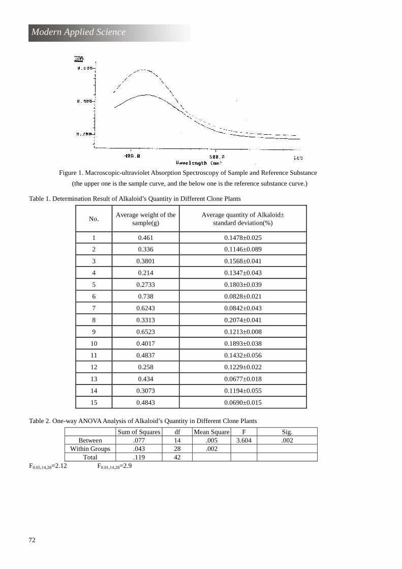
72


Table 1. Determination Result of Alkaloid’s Quantity in Different Clone Plants

No. Average weight of the

sample(g) Average quantity of Alkaloid±

standard deviation(%)

1 0.461 0.1478±0.025

2 0.336 0.1146±0.089

3 0.3801 0.1568±0.041

4 0.214 0.1347±0.043

5 0.2733 0.1803±0.039

6 0.738 0.0828±0.021

7 0.6243 0.0842±0.043

8 0.3313 0.2074±0.041

9 0.6523 0.1213±0.008

10 0.4017 0.1893±0.038

11 0.4837 0.1432±0.056

12 0.258 0.1229±0.022

13 0.434 0.0677±0.018

14 0.3073 0.1194±0.055

15 0.4843 0.0690±0.015

Table 2. One-way ANOVA Analysis of Alkaloid’s Quantity in Different Clone Plants

Sum of Squares df Mean Square F Sig. Between .077 14 .005 3.604 .002

Within Groups .043 28 .002 Total .119 42

F0.05,14,28=2.12 F0.01,14,28=2.9

Figure 1. Macroscopic-ultraviolet Absorption Spectroscopy of Sample and Reference Substance

(the upper one is the sample curve, and the below one is the reference substance curve.)

Modern Applied Science Contents - Semantic Scholar

Documents

Transcript of Modern Applied Science Contents - Semantic Scholar