Precipitation determines the persistence of hollow Sphagnum species on hummocks
Upload
khangminh22Category
view
0download
0
Biogeosciences, 17, 5693–5719, 2020https://doi.org/10.5194/bg-17-5693-2020© Author(s) 2020. This work is distributed underthe Creative Commons Attribution 4.0 License.
Modelling the habitat preference of two key Sphagnum species ina poor fen as controlled by capitulum water contentJinnan Gong1, Nigel Roulet2, Steve Frolking1,3, Heli Peltola1, Anna M. Laine1,4, Nicola Kokkonen1, andEeva-Stiina Tuittila1
1School of Forest Sciences, University of Eastern Finland, P. O. Box 111, 80101 Joensuu, Finland2Department of Geography, McGill University and Centre for Climate and Global Change Research,Burnside Hall, 805 Sherbrooke Street West Montreal, Montréal, Québec H3A 2K6, Canada3Institute for the Study of Earth, Oceans, and Space, and Department of Earth Sciences,University of New Hampshire, Durham, NH 03824, USA4Department of Ecology and Genetics, University of Oulu, P. O. Box 3000, 90014 Oulu, Finland
Correspondence: Eeva-Stiina Tuittila ([email protected])
Received: 8 September 2019 – Discussion started: 18 November 2019Revised: 26 June 2020 – Accepted: 10 July 2020 – Published: 23 November 2020
Abstract. Current peatland models generally treat vegetationas static, although plant community structure is known to al-ter as a response to environmental change. Because the vege-tation structure and ecosystem functioning are tightly linked,realistic projections of peatland response to climate changerequire the inclusion of vegetation dynamics in ecosys-tem models. In peatlands, Sphagnum mosses are key engi-neers. Moss community composition primarily follows habi-tat moisture conditions. The known species habitat prefer-ence along the prevailing moisture gradient might not di-rectly serve as a reliable predictor for future species compo-sitions, as water table fluctuation is likely to increase. Hence,modelling the mechanisms that control the habitat preferenceof Sphagna is a good first step for modelling community dy-namics in peatlands. In this study, we developed the Peat-land Moss Simulator (PMS), which simulates the commu-nity dynamics of the peatland moss layer. PMS is a process-based model that employs a stochastic, individual-based ap-proach for simulating competition within the peatland mosslayer based on species differences in functional traits. At theshoot-level, growth and competition were driven by net pho-tosynthesis, which was regulated by hydrological processesvia the capitulum water content. The model was tested bypredicting the habitat preferences of Sphagnum magellan-icum and Sphagnum fallax – two key species representing dry(hummock) and wet (lawn) habitats in a poor fen peatland(Lakkasuo, Finland). PMS successfully captured the habitat
preferences of the two Sphagnum species based on observedvariations in trait properties. Our model simulation furthershowed that the validity of PMS depended on the interspe-cific differences in the capitulum water content being cor-rectly specified. Neglecting the water content differences ledto the failure of PMS to predict the habitat preferences ofthe species in stochastic simulations. Our work highlights theimportance of the capitulum water content with respect to thedynamics and carbon functioning of Sphagnum communitiesin peatland ecosystems. Thus, studies of peatland responsesto changing environmental conditions need to include capitu-lum water processes as a control on moss community dynam-ics. Our PMS model could be used as an elemental designfor the future development of dynamic vegetation models forpeatland ecosystems.
1 Introduction
Peatlands have important roles in the global carbon cycle, asthey store about 30 % of the world’s soil carbon (Gorham,1991; Hugelius et al., 2013). Environmental changes, suchas climate warming and land use changes, are expectedto impact the carbon functioning of peatland ecosystems(Tahvanainen, 2011). Predicting the functioning of peatlandsunder environmental change conditions requires models toquantify the interactions among ecohydrological, ecophys-
Published by Copernicus Publications on behalf of the European Geosciences Union.

5694 J. Gong et al.: Modelling habitat preference
iological, and biogeochemical processes. These processesare known to be strongly regulated by vegetation (Riutta etal., 2007; Wu and Roulet, 2014), which can change overdecadal timescales under changing hydrological conditions(Tahvanainen, 2011). Peatland models have generally con-sidered vegetation structure in an unrealistic manner: as astatic component (e.g. Frolking et al., 2002; Wania et al.,2009). The recent regional-scale peatland model developedby Chaudhary et al. (2017) includes dynamic vegetationshifts among a single moss plant functional type (PFT) andfour vascular PFTs; however, in order to support realisticpredictions of peatland functioning and global biogeochemi-cal cycles, the mechanisms that drive changes in moss com-munity structure need to be identified and integrated withecosystem processes.
A major fraction of peatland biomass is formed by Sphag-num mosses (Hayward and Clymo, 1983; Vitt, 2000). Al-though individual Sphagnum species often have narrow habi-tat niches (Johnson et al., 2015), different Sphagnum speciesreplace each other along the water table gradient; there-fore, as a genus, Sphagnum species are spread across awide range of water table conditions (Rydin and McDonald,1985; Andrus, 1986; Rydin, 1993; Laine et al., 2009). Thespecies composition of the Sphagnum community stronglyaffects ecosystem processes such as carbon sequestration andpeat formation through interspecific variability in speciestraits including the photosynthetic potential and litter qual-ity (Clymo, 1970; O’Neill, 2000; Vitt, 2000; Turetsky, 2003).The Sphagnum biomass and litter production gradually raisesthe moss carpet, which feeds back into the species compo-sition (Robroek et al., 2009). Hence, modelling the mosscommunity dynamics is fundamental for predicting temporalchanges in peatland vegetation. As the distribution of Sphag-num species primarily follows the variability in the peatlandwater table (Andrus, 1986; Väliranta et al., 2007), modellingthe habitat preference of Sphagnum species along a moisturegradient could be a good first step in predicting moss com-munity dynamics (Blois et al., 2013).
For a given Sphagnum species, the optimal habitat repre-sents the environmental conditions for it to achieve higherrates of net photosynthesis and shoot elongation than itspeers (Titus and Wagner, 1984; Rydin and McDonald, 1985;Rydin, 1997; Robroek et al., 2007a; Keuper et al., 2011). Thecapitulum water content and water storage, which are deter-mined by the balance between the evaporative loss and wa-ter gains from capillary rise and precipitation, represent oneof the most important controls on net photosynthesis (Titusand Wagner, 1984; Murray et al., 1989; Van Gaalen et al.,2007; Robroek et al., 2009). To quantify the water processesin mosses, hydrological models have been developed to sim-ulate the water movement between the moss carpet and thepeat underneath, as regulated by the variations in meteoro-logical conditions and energy balance (Price, 2008; Price andWhittington, 2010). On the other hand, experimental workhas addressed the species-specific responses of net photosyn-
thesis to changes in the capitulum water content (Titus andWagner, 1984; Hájek and Beckett, 2008; Schipperges andRydin, 1998) and light intensity (Rice et al., 2008; Laine etal., 2011; Bengtsson et al., 2016). Net photosynthesis and hy-drological processes are linked via capitulum water retention,which controls the response of the capitulum water contentto water potential changes (Jassey and Signarbieux, 2019).However, these mechanisms have not been integrated withecosystem processes in model simulations.
Along with the capitulum water processes, modelling thehabitat preference of Sphagna requires the quantification ofthe competition among mosses, i.e. the “race for space” (Ry-din, 1993, 1997; Robroek et al., 2007a; Keuper et al., 2011):Sphagnum shoots can form new capitula and spread later-ally if there is space available. This reduces or eliminatesthe light source for any plant that is buried by its peers(Robroek et al., 2009). As the competition occurs betweenneighbouring shoots, its modelling requires downscaling in-terlinked water–energy processes from the ecosystem to theshoot level. Thus, Sphagnum competition needs to be mod-elled as spatial processes, considering the fact that spatial co-existence and the variations in functional traits among shootindividuals may impact the community dynamics (Bolker etal., 2003; Amarasekare, 2003). However, coexistence gener-ally relies on simple coefficients to describe the interactionsamong individuals (e.g. Czárán and Iwasa, 1998; Andersonand Neuhauser, 2000; Gassmann et al., 2003; Boulangeat etal., 2018) and is consequently decoupled from environmentalfluctuation or the stochasticity of biophysiological processes.
This study aims to develop and test a model, the PeatlandMoss Simulator (PMS), to simulate community dynamicswithin the peatland moss layer that results in realistic habi-tat preference of Sphagnum species along a moisture gradi-ent. In PMS, community dynamics is driven by Sphagnumphotosynthesis. Photosynthesis, in turn, is regulated by ca-pitulum water retention through the capitulum moisture con-tent. Therefore, we hypothesize that the water retention ofthe capitula is the mechanism driving moss community dy-namics. We test the model validity using data from an ex-periment based on two Sphagnum species that have differentpositions along the moisture gradient in the same peatlandsite. If our hypothesis holds, the model will (1) correctly pre-dict the competitiveness of the two species in wet and dryhabitats and (2) fail to predict competitiveness if the capitu-lum water retention and water content of the two species arenot correctly specified.
2 Materials and methods
2.1 Study site
The peatland site being modelled is located in Lakkasuo,Orivesi, Finland (61◦47′ N; 24◦18′ E). The site is a poor fenfed by mineral inflows from a nearby esker (Laine et al.,
Biogeosciences, 17, 5693–5719, 2020 https://doi.org/10.5194/bg-17-5693-2020

J. Gong et al.: Modelling habitat preference 5695
2004). Most of the site is formed by lawns dominated bySphagnum recurvum complex (Sphagnum fallax accompa-nied by Sphagnum flexuosum and Sphagnum angustifolium)and Sphagnum papillosum. Less than 10 % of the surfaceis occupied by hummocks, inhabited by Sphagnum magel-lanicum and Sphagnum fuscum, which are 15–25 cm higherthan the lawn surfaces. Both microforms are covered bycontinuous Sphagnum carpet with a sparse vascular plantcover (12 % Carex cover on average), which spread homo-geneously over the topography. The annual mean water ta-ble was 15.6±5.0 cm deep at the lawn surface (Kokkonen etal., 2019). More information about the site can be found inKokkonen et al. (2019).
2.2 Model outline
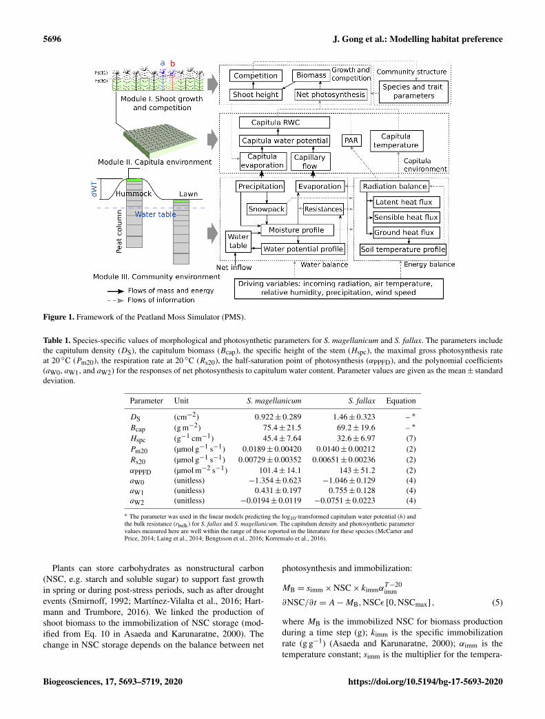
The Peatland Moss Simulator (PMS) is a process-based,stochastic model that simulates the temporal dynamics of aSphagnum community as driven by variations in precipita-tion, irradiation, and energy flow with individual-based inter-actions (Fig. 1). In PMS, the studied ecosystem is seen as adual-column system consisting of hydrologically connectedhabitats of hummocks and lawns (community environment inFig. 1). For each habitat type, the community area is down-scaled to two-dimensional cells representing the scale of in-dividual shoots (i.e. 1 cm2). Each grid cell can be occupiedby one capitulum from a single Sphagnum species. The com-munity dynamics, i.e. the changes in species abundances, aredriven by the growth and competition of Sphagnum shoots atthe grid-cell level (Module I in Fig. 1). These processes areregulated by the grid-cell-specific conditions of water and en-ergy (Module II in Fig. 1), which are derived from the com-munity environment (Module III in Fig. 1).
In this study, we focused on developing modules I andII (Sect. 2.3) and employed an available soil–vegetation–atmosphere transport (SVAT) model (Gong et al., 2013,2016) to describe the water–energy processes for ModuleIII (Appendix A). We assumed that the temporal variation inthe water table was similar in lawns and hummocks and thatthe hummock–lawn differences in the water table (dWT inFig. 1) followed their difference in surface elevations (Wil-son, 2012). At the grid-cell level, the photosynthesis of ca-pitula drove the biomass growth and elongation of shoots,which led to the competition between adjacent grid cells. Thenet photosynthesis rate was controlled by the capitulum wa-ter content, Wcap, which was defined by the capitulum waterretention in relation to the water potential, h (Sect. 2.4). Thevalues for functional traits that regulate the growth and com-petition processes were randomly selected within their nor-mal distribution measured in the field (Sect. 2.4). Unknownparameters that related the lateral water flows of the site areestimated using a machine-learning approach (Sect. 2.5). Fi-nally, a Monte Carlo simulation was used to support the anal-ysis of the habitat preferences of Sphagnum species and hy-
pothesis tests (Sect. 2.6). The list of symbols used is given inAppendix E.
2.3 Model development
2.3.1 Calculating shoot growth and competition ofSphagnum mosses (Module I)
Calculation of Sphagnum growth
To model the grid-cell biomass production and height incre-ment, we assumed that capitula were the main parts of theshoots responsible for photosynthesis and the production ofnew tissues, instead of the stem sections underneath. We em-ployed a hyperbolic light-saturation function (Larcher, 2003)to calculate the net photosynthesis, which was parameter-ized based on empirical measurements made from the tar-get species collected from the study site (see Appendix B formaterials and methods):
A20 =
(Pm20×PPFDαPPFD+PPFD
−Rs20
)×Bcap, (1)
where subscript 20 denotes the variable value measured at20 ◦C; Rs is the mass-based respiration rate (µmol g−1 s−1);Pm is the mass-based rate of maximal gross photosynthe-sis (µmol g−1 s−1); PPFD is the photosynthetic photon fluxdensity (µmol m−2 s−1); Bcap is the capitulum biomass; andαPPFD is the half-saturation point (µmol m−2 s−1) for photo-synthesis.
By adding multipliers for the capitula water content (fW)and temperature (fT) to Eq. (1), the net photosynthesis rateA (µmol m−2 s−1) was calculated as follows:
A=
[Pm20×PPFDαPPFD+PPFD
fT (T )−Rs20fR (T )
]×Bcap
× fW(Wcap
), (2)
where fW(Wcap) describes the responses of A to the capitu-lum water content, Wcap; and fT(T ) describes the responsesof Pm to the capitulum temperature T (Korrensalo et al.,2017). fW(Wcap) was estimated based on the empirical mea-surements (see Sect. 2.4 and Appendix B). The temperatureresponse fR(T ) is a Q10 function that describes the temper-ature sensitivity of Rs (Frolking et al., 2002):
fR (T )=Q(T−Topt)/1010 , (3)
where Q10 is the sensitivity coefficient; T is the capitulumtemperature (◦C); and Topt (20 ◦C) is the reference tempera-ture of respiration.
The response of A to Wcap (fW(Wcap); Eq. 2) was de-scribed as a second-order polynomial function:
fW(Wcap)= aW0+ aW1×Wcap+ aW2×W2cap, (4)
where aW0, aW1, and aW2 are coefficients.
https://doi.org/10.5194/bg-17-5693-2020 Biogeosciences, 17, 5693–5719, 2020
5696 J. Gong et al.: Modelling habitat preference
Figure 1. Framework of the Peatland Moss Simulator (PMS).
Table 1. Species-specific values of morphological and photosynthetic parameters for S. magellanicum and S. fallax. The parameters includethe capitulum density (DS), the capitulum biomass (Bcap), the specific height of the stem (Hspc), the maximal gross photosynthesis rateat 20 ◦C (Pm20), the respiration rate at 20 ◦C (Rs20), the half-saturation point of photosynthesis (αPPFD), and the polynomial coefficients(aW0, aW1, and aW2) for the responses of net photosynthesis to capitulum water content. Parameter values are given as the mean± standarddeviation.
Parameter Unit S. magellanicum S. fallax Equation
DS (cm−2) 0.922± 0.289 1.46± 0.323 – ∗
Bcap (g m−2) 75.4± 21.5 69.2± 19.6 – ∗
Hspc (g−1 cm−1) 45.4± 7.64 32.6± 6.97 (7)Pm20 (µmol g−1 s−1) 0.0189± 0.00420 0.0140± 0.00212 (2)Rs20 (µmol g−1 s−1) 0.00729± 0.00352 0.00651± 0.00236 (2)αPPFD (µmol m−2 s−1) 101.4± 14.1 143± 51.2 (2)aW0 (unitless) −1.354± 0.623 −1.046± 0.129 (4)aW1 (unitless) 0.431± 0.197 0.755± 0.128 (4)aW2 (unitless) −0.0194± 0.0119 −0.0751± 0.0223 (4)
∗ The parameter was used in the linear models predicting the log10-transformed capitulum water potential (h) andthe bulk resistance (rbulk) for S. fallax and S. magellanicum. The capitulum density and photosynthetic parametervalues measured here are well within the range of those reported in the literature for these species (McCarter andPrice, 2014; Laing et al., 2014; Bengtsson et al., 2016; Korrensalo et al., 2016).
Plants can store carbohydrates as nonstructural carbon(NSC, e.g. starch and soluble sugar) to support fast growthin spring or during post-stress periods, such as after droughtevents (Smirnoff, 1992; Martínez-Vilalta et al., 2016; Hart-mann and Trumbore, 2016). We linked the production ofshoot biomass to the immobilization of NSC storage (mod-ified from Eq. 10 in Asaeda and Karunaratne, 2000). Thechange in NSC storage depends on the balance between net
photosynthesis and immobilization:
MB = simm×NSC× kimmαT−20imm
∂NSC/∂t = A−MB,NSCε [0,NSCmax] , (5)
where MB is the immobilized NSC for biomass productionduring a time step (g); kimm is the specific immobilizationrate (g g−1) (Asaeda and Karunaratne, 2000); αimm is thetemperature constant; simm is the multiplier for the tempera-
Biogeosciences, 17, 5693–5719, 2020 https://doi.org/10.5194/bg-17-5693-2020

J. Gong et al.: Modelling habitat preference 5697
ture threshold, where simm = 1 when T > 5 ◦C but simm = 0if T ≤ 5 ◦C; and NSCmax is the maximal NSC concentra-tion in Sphagnum biomass (Turetsky et al., 2008). The tim-ing of growth is controlled by a temperature threshold andNSC availability. Growth occurs when T > 5 ◦C and NSC isabove zero. The dynamics of NSC storage is related to thewater content (WC) through net photosynthesis.
The increase in shoot biomass drove the shoot elongation:
∂Hc/∂t =MB
HspcSc, (6)
where Hc is the shoot height (cm); Hspc is the biomass den-sity of Sphagnum stems (g m−2 cm−1); and Sc is the area ofa cell (m2).
Calculation of Sphagnum competition and communitydynamics
To simulate the competition among Sphagnum shoots, wefirst compared Hc of each grid cell (source grid cell, i.e. gridcell a in Fig. 1) to its four neighbouring cells and marked theone with the lowest position (e.g. grid cell b in Fig. 1) as thetarget of spreading. The spreading of shoots from a source toa target grid cell occurred when the following criteria werefulfilled: (i) the height difference between the source and tar-get grid cells exceeded a threshold value; (ii) NSC accumu-lation in the source grid cell was large enough to support thegrowth of new capitula in the target grid cell; and (iii) thecapitula in the source grid cell could split once per year atmost.
The height difference threshold in rule (i) was set equal tothe mean diameter of the capitula in the source cell, basedon the assumption that the shape of a capitulum was spheri-cal. When shoots spread, the species type and model param-eters in the target grid cell were overwritten by those in thesource grid cell, assuming the mortality of shoots originallyin the target cell. During the spreading, the NSC storage wastransferred from the source cell to the target cell to form newcapitula. In cases where spreading did not take place, the es-tablishment of new shoots from spores could maintain thecontinuity of the Sphagnum carpet at the site. During the es-tablishment from spores, which was rare and occurred duringthe first years of simulation, the traits of Sphagnum specieswere randomized within their normal distribution measuredin the field.
2.3.2 Calculating the grid-cell-level dynamics ofenvironmental factors (Module II)
Module II computes grid-cell values of Wcap, PPFD, and Tfor Module I. The cell-level PPFD and T were assumed to beequal to the community means, which were solved using theSVAT scheme in Module III (Appendix A). The community-level evaporation rate (E) was partitioned to the cell level
(Ei) as follows:
Ei = E×
(Svirbulk,i
)/∑(Svirbulk,i
), (7)
where rbulk,i is the bulk surface resistance of cell i, whichis as a function (rbulk,i = fr(hi)) of the grid-cell-based wa-ter potential hi , capitulum biomass (Bcap), and shoot density(DS) based on the empirical measurements (Appendix B).Svi was the evaporative area, which was related to the heightdifferences among adjacent grid cells:
Svi = Sci + lc∑
j
(Hci −Hcj
), (8)
where lc is the width of a grid cell (cm); and subscript j de-notes the four nearest neighbouring grid cells. In this way,changes in the height difference between the neighbouringshoots feed back to affect the water conditions of the gridcells via an alteration of the evaporative surface area.
The grid-cell-level changes in the capitula water potential(hi) were driven by the balance between the evaporation (Ei)and the upward capillary flow to capitula:
∂hi =Km
Ci
[(hi −hm)
0.5zm− 1−Ei
], (9)
where hm is the water potential of the living moss layer,solved in Module III (Appendix A); zm is the thickness ofthe living moss layer (zm = 5 cm); Km is the hydraulic con-ductivity of the moss layer and is set to be the same for eachgrid cell; and Ci is the cell-level specific water uptake capac-ity (Ci = ∂Wcap,i/∂hi). ∂Wcap,i/∂hi could be derived fromthe capitulum water retention function hi = fh(Wcap). Wcap,which affects the calculation of net photosynthesis throughfW(Wcap), can then be estimated from hi using the fh(Wcap)
function (Table B2, Table B3).
2.4 Model parameterization
2.4.1 Selection of Sphagnum species
We chose S. fallax and S. magellanicum, which form 63 %of total plant cover at the study site at Lakkasuo (Kokkonenet al., 2019), as the target species representing the lawn andhummock habitats respectively. These species share a simi-lar niche along soil pH and nutrient richness gradients (Wo-jtun et al., 2003), but they are discriminated by their watertable level preferences (Laine et al., 2004): while S. fallaxis commonly found close to the water table (Wojtun et al.,2003), S. magellanicum can occur along a wider range of thewet–dry gradient, from intermediately wet lawns to dry hum-mocks (Rice et al., 2008; Kyrkjeeide, et al., 2016; Korresaloet al., 2017). Thus, the transition from S. fallax to S. mag-ellanicum along the wet–dry gradient indicates the decreas-ing competitiveness of S. fallax with S. magellanicum with alowering water table.
https://doi.org/10.5194/bg-17-5693-2020 Biogeosciences, 17, 5693–5719, 2020
5698 J. Gong et al.: Modelling habitat preference
Table 2. Parameters values for the SVAT simulations (Module III).The parameters include the saturated hydraulic conductivity (Ksat),the water retention parameters of water retention curves (α and n),the saturated water content (θs), the permanent wilting point wa-ter content (θr), the snow layer surface albedos (as, al), the thermalconductivity (KT), the specific heat (CT), and the maximal non-structural carbon (NSC) concentration (NSCmax).
Parameter Value Equation Source
Ksat 162 A6 McCarter and Price (2014)n 1.43 A5 McCarter and Price (2014)α 2.66 A5 McCarter and Price (2014)θs 0.95a A5 Päivänen (1973)θr 0.071b A5 Weiss et al. (1998)as 0.15 A9 Runkle et al. (2014)al 0.02 A10 Thompson et al. (2015)KT,water 0.57 A4 Letts et al. (2000)KT,ice 2.20 A4 Letts et al. (2000)KT,org 0.25 A4 Letts et al. (2000)CT,water 4.18 A3 Letts et al. (2000)CT,ice 2.10 A3 Letts et al.. (2000)CT,org 1.92 A3 Letts et al. (2000)NSCmax 0.045 6 Turetsky et al. (2008)
a The value was calculated from bulk density (ρbulk) as θs = 97.95− 79.72ρbulkfollowing Päivänen (1973); b The value was calculated as θr = 4.3+ 67ρbulkfollowing Weiss et al. (1998).
2.4.2 Parameterization of morphological traits, netphotosynthesis, and capitulum water retention
We empirically quantified the morphological traits of the ca-pitulum density (DS; shoots cm−2), the biomass of capitula(Bcap; g m−2), the biomass density of living stems (Hspc;g cm−1 m−2), the net photosynthesis parameters (Pm20, Rs20,and αPPFD), and the water retention properties, i.e. fh(Wcap)and fr(h) (Eqs. 8 and 10), for the two Sphagnum species(see Appendix B for methods). The values (mean±SD) ofthe morphological parameters, the photosynthetic parame-ters, and the polynomial coefficients (aW0, aW1, and aW2;Eq. 3) are listed in Table B1 in Appendix B. For each param-eter, a random value was initialized for each cell based on themeasured means and SD, assuming that the variation in theparameter values is normally distributed.
We noticed that the fitted fW(Wcap) was meaningful whenWcap was below the optimal water content for photosynthesis(Wopt =−0.5aW1/aW2). If Wcap >Wopt, photosynthesis de-creased linearly with increasing Wcap, as it is limited by thediffusion of CO2 (Schipperges and Rydin, 1998). In that case,fW(Wcap) was calculated following Frolking et al. (2002):
fW(Wcap
)= 1− 0.5
Wcap−Wopt
Wmax−Wopt, (10)
where Wmax is the maximum water content of the capitula.It is known that Wmax is around 25–30 g g−1 (e.g. Schip-
perges and Rydin, 1998) or about 0.31–0.37 cm3 cm−3 in
terms of the volumetric water content (assuming a 75 g m−2
capitula biomass and a 0.6 cm high capitula layer). Thisrange is broadly lower than the saturated water content of themoss carpet (> 0.9 cm3 cm−3, McCarter and Price, 2014).Consequently, we used the following equation to convertthe volumetric water content to the capitulum water con-tent (RWC), when hi was higher than the boundary valueof −104 cm:
Wcap =min(Wmax,θm/
(Hcap×Bcap× 10−4
)), (11)
where Wmax is the maximum water content and is set to25 g g−1 for both species; θm is the volumetric water con-tent of the moss layer; and Hcapis the height of the capitulaand is set to 0.6 cm (Hájek and Beckett, 2008).
2.5 Model calibration for lateral water influence
We used a machine-learning approach to estimate the influ-ence of the upstream area on the water balance of the site.The rate of net inflow (I , see Eq. A18 in Appendix A) wasdescribed as a function of Julian day (JD), assuming thatthe inflow was maximum after the spring thaw and then de-creased linearly with time:
Ij = (aN× JD+ bN)×Ksj JD> JDthaw, (12)
where subscript j denotes the peat layers under the watertable; Ks is the saturated hydraulic conductivity; JDthaw isthe Julian day that thawing completed; and aN and bN areparameters.
We simulated water table changes using climatic scenariosfrom the Weather Generator (Appendix A). During calibra-tion, the community compositions were set to remain con-stant, such that S. magellanicum fully occupied the hummockhabitat whereas S. fallax fully occupied the lawn habitat. Thesimulated multiyear means of weekly water table values werecompared to the weekly mean water table values observed atthe site during the years 2001, 2002, 2004, and 2016. Thecost function for the learning process was based on the sumof squared error (SSE) of the simulated water table:
SSE=6(WTsk −WTmk
)2, (13)
where WTm is the measured multiyear weekly mean of thewater table; WTs is the simulated multiyear weekly mean ofthe water table; and subscript k denotes the week of the yearwhen the water table was sampled.
The values of aN and bN were estimated using the gradientdescent approach (Ruder, 2016) by minimizing the SSE in aNand bN in Eq. (12):
XN (j) :=XN (j)−0∂SSE∂XN (j)
, (14)
where 0 is the learning rate (0 = 0.1). Appendix D showsthe simulated water table with the calibrated inflow term I
compared with the measured values from the site.
Biogeosciences, 17, 5693–5719, 2020 https://doi.org/10.5194/bg-17-5693-2020

J. Gong et al.: Modelling habitat preference 5699
2.6 Model-based analysis
First, we examined the ability of the model to capture thepreference of S. magellanicum for the hummock environmentand the preference of S. fallax for the lawn environment (Test1). For both species, the probability of occupation was initial-ized as 50 % in a cell, and the distribution of the species inthe communities were randomly patterned. Monte Carlo sim-ulations (40 replicates) were carried out with a time step of30 min. A simulation length of 15 years was selected basedon preliminary studies in order to cover the major interval ofchange and to ease computational demand. Biomass growth,stem elongation, and the spreading of shoots were simulatedon a daily basis. The establishment of new shoots in deacti-vated cells was calculated at the end of each simulation year.We then assessed if the model could capture the dominanceof S. magellanicum in the hummock communities and thedominance of S. fallax in lawn communities. The simulatedannual height increments of mosses were compared to thevalues measured for each community type. To measure mossvertical growth in the field, we deployed 20 cranked wireson S. magellanicum-dominated hummocks and 15 crankedwires on S. fallax-dominated lawns in 2016. Each crankedwire was a piece of metal wire attached to plastic brushes atthe side that was anchored into the moss carpet (e.g. Clymo,1970; Holmgren et al., 2015). Annual vertical growth (dH)was determined by measuring the change in the exposed wirelength above the moss surface from the beginning to the endof growing season.
Second, we tested the robustness of the model to the un-certainties in a set of parameters (tests 2–4). In Test 2, wefocused on parameters that were closely linked to hydrologyand growth calculations but were roughly parameterized (e.g.kimm, raero) or adopted as a priori from other studies (e.g.Ksat, α, n, NSCmax; see Table 2). One at a time, each pa-rameter value was adjusted by +10 % or −10. A total of 40Monte Carlo simulations were run using the same runtimesettings as in Test 1. The simulated means of cover were thencompared to those calculated without the parameter adjust-ment.
Tests 3 and 4 were then carried out to test whether themodel could correctly predict the competitiveness of thespecies in dry and wet habitats if the species-specific trendsin the capitulum water content were not correctly specified.For both species, we set the values of parameters controllingthe water retention (i.e. Bcap and DS; Appendix B) and thewater-stress effects on net photosynthesis (i.e. Wcap; Eq. 4)to be the same as those for S. magellanicum (Test 3) or sameas those for S. fallax (Test 4). Our hypothesis would be sup-ported if removing the interspecific differences in RWC re-sponses led to the failure to predict the habitat preferences ofthe species.
We implemented tests 5 and 6 to investigate the impor-tance of parameters that directly control the species ability toovergrow another species with a more rapid height increment
Table 3. The results from Test 2, which addressed the robustness ofthe model to the uncertainties in a set of parameters. Each parameterwas increased or decreased by 10 %. The model was run for S. mag-ellanicum and S. fallax in their preferential habitats. The differencein mean cover between simulations as a function of changed or un-changed parameter values is given; the standard deviations (SD) ofthe means are given in parentheses. The parameters include the spe-cific immobilization rate (kimm), the maximal nonstructural carbon(NSC) concentration (NSCmax), the hydraulic conductivity of themoss layer (Km), the hydraulic conductivity of the peat layer (Kh),the water retention parameters of the water retention curves (α andn), the snow layer surface albedo (as), and the aerodynamic resis-tance (raero).
Change in Equation Changes in simulated cover, % (SD)
parameter S. magellanicum S. fallaxvalue (hummock) (lawn)
kimm+ 10 % 5 −1.2 (3.5) −3.5 (3.8)kimm−10 % +2.7 −5.0 (3.4)
NSCmax+ 10 % 6 +4.5 +0.7NSCmax −10 % −0.7 (4.0) −4.8 (4.5)
Km+ 10 % 10 +1.0 −1.7 (2.3)Km− 10 % −1.7 (2.7) +4.1
Kh+ 10 % A1 −1.1 (2.0) +1.1Kh− 10 % −1.8 (3.1) −0.5 (2.7)
n+ 10 % A5 −1.6 (3.2) −3.2 (3.2)n− 10 % −9.4 (3.6) −0.3 (2.9)
α+ 10 % A5 −0.5 (2.7) −0.3 (2.3)α− 10 % −1.3 (3.6) +3.2
as+ 10 % A9 −2.2 (3.8) +0.6as− 10 % +3.3 +1.2
raero+ 10 % A14, −2.1 (3.4) +0.3raero− 10 % A15 −3.8 (4.4) +2.3
(i.e. Pm20, Rs20, αPPFD, andHspec) under lawn and hummockconditions. We eliminated the species differences in the pa-rameter, so that the values were the same as those in S. mag-ellanicum (Test 5) or the same as those in S. fallax (Test 6).The effects of the manipulation were compared with thosefrom tests 3 and 4. For tests 3–6, 80 respective Monte Carlosimulations were run using the set-ups described in Test 1.
Tests 7 and 8 were implemented to separate the effects ofphotosynthetic water-response parameters from the effects ofthe capitula water retention. We set the photosynthetic water-response parameters to be the same as those in S. magellan-icum (Test 7) or the same as those in S. fallax (Test 8). Asour model aimed to couple the environmental fluctuationsand stochasticity of ecosystem processes, we further testedthe model responses to the absence of environmental fluctu-ations (Test 9) or the absence of stochasticity in model pa-rameters (Test 10). In Test 9, monthly mean values of meteo-rological variables were used to drive the model simulation.In Test 10, we removed the stochasticity of model parame-ters and assigned an average value to each parameter of grid
https://doi.org/10.5194/bg-17-5693-2020 Biogeosciences, 17, 5693–5719, 2020

5700 J. Gong et al.: Modelling habitat preference
Table 4. Result from tests 7–10, which addressed the importance ofmeteorological fluctuations, the stochasticity of model parameters,and the photosynthetic water response. In Test 7, monthly mean val-ues of meteorological variables were used to drive the model simu-lation. In Test 8, the stochasticity of model parameters was removed,and the average values were used for parameters at the grid-celllevel. In tests 9 and 10, the photosynthetic water-response parame-ters (i.e. aW0, aW1, and aW2; see Table 1) were set to be the same asthose for S. magellanicum (Test 9) or the same as those for S. fallax(Test 10). The mean cover of S. magellanicum on hummocks andthe cover of S. fallax on lawns after the 15-year simulation periodsare listed in Table 4.
Test S. magellanicum S. fallax(hummock) (lawn)
7 73 % 96 %8 90 % 72 %9 14 % 100 %10 100 % 100 %
cells. For tests 7–10, 40 respective Monte Carlo simulationswere run using the set-ups described in Test 1.
3 Results
3.1 Simulating the habitat preferences of Sphagnumspecies as affected by the capitulum water contenttraits
Test 1 demonstrated the ability of the model to capture thepreference of S. magellanicum for the hummock environ-ment and the preference of S. fallax for the lawn environment(Fig. 2a). The simulated annual changes in species coverwere greater in lawn habitats than in hummock habitats dur-ing the first 5 simulation years. The changes in lawn habi-tats slowed down around year 10, and the cover of S. fallaxplateaued at around 95± 2.8 % (mean± standard error). Incontrast, the cover of S. magellanicum on hummocks con-tinued to grow until the end of the simulation and reached83± 3.1 %. In the lawn habitats, the cover of S. fallax in-creased in all Monte Carlo simulations, and the species occu-pied all grid cells in 70 % of the simulations. In the hummockhabitats, the cover of S. magellanicum increased in 91 % ofMonte Carlo simulations, and it formed a monocultural com-munity in 16 % of simulations (Fig. 2b). The vertical growthof Sphagnum mosses was significantly greater in lawn habi-tats than in hummock habitats (P < 0.01). The ranges of sim-ulated vertical growth agreed well with the observed valuesfrom field measurement for both species (Fig. 2c).
Figure 2. Testing the ability of PMS to predict the habitat prefer-ence of Sphagnum magellanicum and S. fallax (Test 1). The hum-mock and lawn habitats were differentiated by the water table depth,the surface energy balances, and the capitulum water potential inthe model simulations. At the beginning of the simulation, thecover of the two species was set to be equal and it was allowedto develop with time. (a) The annual development of the relativecover (mean and standard error) of the two species in hummockand lawn habitats, (b) the cumulative probability distribution of thecover of the two species at the end of the 15-year period based on40 Monte Carlo simulations, and (c) the simulated and measuredmeans of the annual vertical growth of Sphagnum surfaces in theirnatural habitats (hummock and lawn).
3.2 Testing model robustness
Test 2 addressed the model robustness to the uncertaintiesin several parameters that were closely linked to hydrologyand growth calculations. Modifying most of the parametervalues by +10 % or −10 % yielded marginal changes in themean cover of species in either hummock or hollow habitats(Table 3). Reducing the moss carpet and the peat hydraulicparameter n had stronger impacts on S. fallax cover in hum-
Biogeosciences, 17, 5693–5719, 2020 https://doi.org/10.5194/bg-17-5693-2020

J. Gong et al.: Modelling habitat preference 5701
mock habitats than in lawn habitats. Nevertheless, changesin simulated cover that were caused by parameter manipula-tions were generally smaller than the standard deviations ofthe means, i.e. fitting into the random variation.
3.3 Testing the controlling role of the capitulum watercontent on community dynamics
In tests 3 and 4, the model incorrectly predicted the com-petitiveness of the two test species when the interspecificdifferences in the capitulum water content were eliminated.In both tests, S. fallax became dominant in all habitats. Theuse of water-response characteristics from S. magellanicumfor both species (Test 3) led to the faster development ofS. fallax cover and higher coverage at the end of simula-tion (Fig. 3a) compared with the simulation results wherethe water-response characteristics from S. fallax were usedfor both species (Test 4, Fig. 3b). The pattern was more pro-nounced in hummock than in lawn habitats.
In tests 5 and 6, the species differences in the growth-related parameters were eliminated. However, the model stillpredicted the dominance of S. fallax and S. magellanicumin lawn and hummock habitats respectively (Fig. 4). The in-crease in the mean cover of S. magellanicum was especiallyfast in the hummock habitat in comparison to the results ofthe unchanged model from Test 1 (Fig. 2a). In lawns, the useof S. fallax growth parameters for both species gave strongercompetitiveness to S. magellanicum (Fig. 4b) than using theS. magellanicum parameters (Fig. 4a). In tests 7 and 8, ignor-ing the interspecific differences in the photosynthetic water-response parameters did not change the simulated habitatpreferences of S. fallax and S. magellanicum (Table 4). Us-ing the water-response parameters of S. fallax decreased themean cover of S. fallax in lawns but increased the cover ofS. magellanicum on hummocks. In contrast, using the water-response parameters of S. magellanicum increased the meancover of S. fallax in lawns but decreased the cover of S. mag-ellanicum on hummocks.
3.4 Testing the effects of environmental fluctuationsand the stochasticity of ecosystem processes oncommunity dynamics
In Test 9, the model failed to simulate the preference ofS. magellanicum for hummocks (Table 4) if the environmen-tal fluctuation was ignored. However, the simulated cover ofS. fallax in lawns was higher compared with the unchangedcondition (i.e. Test 1). Using the mean value for each modelparameters led to monocultural community, i.e. S. magellan-icum occupied 100 % of the hummock area whereas S. fallaxtook over lawns completely.
4 Discussion
In peatland ecosystems, Sphagna are keystone species dis-tributed primarily along the hydrological gradient (e.g. An-drus, 1986; Rydin, 1986). In a context where substantialchange in peatland hydrology is expected under a changingclimate in northern areas (e.g. longer snow-free season, lowersummer water table, and more frequent droughts), there is apressing need to understand how peatland plant communitiescould react and how Sphagnum species could redistribute un-der habitat changes. In this work, we developed the PeatlandMoss Simulator (PMS), a process-based stochastic model,to simulate the competition between S. magellanicum andS. fallax, two key species representing dry (hummock) andwet (lawn) habitats in a poor fen peatland. We empiricallyshowed that these two species differed in characteristics thatlikely affect their competitiveness along a moisture gradient.
Capitulum water retention for the lawn-preferring species(S. fallax) was weaker than that for the hummock-preferringspecies (S. magellanicum). Compared with S. magellanicum,the capitula of S. fallax held less water at saturation and thewater content decreased more rapidly with dropping waterpotential. Hence, S. fallax would dry faster than S. magellan-icum under the same rate of water loss. Moreover, the watercontent in S. fallax capitula was less resistant to evaporation.These differences indicated that it is harder for S. fallax ca-pitula to buffer evaporative water loss and, therefore, avoidor delay desiccation. Similar differences between hummockand hollow species have been in previous studies (Titus andWagner, 1984; Rydin and McDonald, 1985). In addition, thenet photosynthesis of S. fallax is more sensitive to changes inthe capitulum water content than S. magellanicum, as seen bythe steeper decline in photosynthesis with decreasing watercontent (Fig. B2c). Consequently, the growth of S. fallax ismore likely to be slowed down by dry periods, during whichthe capillary water cannot fully compensate for the evapora-tive loss (Robroek et al., 2007b), making it less competitivein habitats prone to desiccation.
The PMS successfully captured the habitat preferences ofthe two Sphagnum species (Test 1): starting from a mixedcommunity with equal probabilities for both species, thelawn habitats with the shallower water table were eventuallydominated by the typical lawn species S. fallax, whereas thehummock habitats, which were 15 cm higher than the lawnsurface, were taken over by S. magellanicum. The low finalcover of S. magellanicum simulated in lawn habitats agreedwell with field observations from our study site, whereS. magellanicum cover was less than 1 % in lawns (Kokko-nen et al., 2019). Conversely, S. fallax was outcompeted byS. magellanicum in the hummock habitats. This result is con-sistent with previous findings that hollow-preferring Sphagnaare less likely to survive in hummock environments withgreater drought pressure (see Rydin, 1985; Rydin et al., 2006;Johnson et al., 2015). The simulated annual height incre-ments of mosses also agreed well with the observed values
https://doi.org/10.5194/bg-17-5693-2020 Biogeosciences, 17, 5693–5719, 2020

5702 J. Gong et al.: Modelling habitat preference
Figure 3. Testing the importance of capitulum water content for the habitat preference of S. magellanicum and S. fallax. The developmentof the relative cover (mean and standard error) were simulated in hummock and lawn habitats over a 15-year time frame for the two species.For both species, parameter values for the capitulum water content, the capitulum biomass (Bcap), and the density (DS) were set to be thesame as those from (a) S. magellanicum (Test 3) or (b) S. fallax (Test 4).
Figure 4. Testing the importance of parameters regulating net photosynthesis and shoot elongation for the habitat preference of S. magellan-icum and S. fallax. The annual development of the relative cover (mean and standard error) of the two species was simulated for hummockand lawn habitats over a 15-year time frame. For both species, the parameter values (i.e. Pm20, Rs20, αPPFD, and Hspec) were set to be thesame as those from (a) S. magellanicum (Test 5) or (b) S. fallax (Test 6).
for both habitat types. Our simulation for lawn habitat showsthat the looser stem structure of S. fallax allows it to allo-cate more of its produced biomass into vertical growth and,therefore, overgrow S. magellanicum, in which new biomassforms a compact stem that is packed with thick fascicles.This finding indicates that PMS can capture the key mech-anisms controlling the growth and competitive interactionsof the Sphagnum species.
Parameter sensitivity testing showed the robustness ofPMS regarding the uncertainties in parameterization, as thesimulated changes in the mean species cover (under 10 %variation in several parameters) were generally less than thestandard deviations of the means. Decreasing the value ofthe hydraulic parameter n (Table 2, Eq. A5) increased thepresence of S. fallax in the hummock habitats. This was ex-pected because n is a scaling factor and its changes are conse-quently magnified: a lower n value will lead to a higher watercontent in the unsaturated layers above the water table (vanGenuchten, 1980), which allows Sphagna that are adaptedto wet environments to survive dry conditions (Hayward and
Clymo, 1982; Robroek et al., 2007b; Rice et al., 2008). Incontrast, the response of Sphagnum cover to the changes inother hydraulic parameters (i.e. α, n,Kh) was limited in lawnhabitats. This could be due to the relatively shallow watertable in lawns, which was able to maintain sufficient capil-lary rise to the moss carpet and capitula. Decreasing the val-ues of the specific immobilization rate (kimm) and maximalNSC concentration in Sphagnum biomass (NSCmax) mainlydecreased the cover of S. fallax in lawn habitats, which isconsistent with the importance of biomass production toSphagna in high-moisture environments (e.g. Rice et al.,2008; Laine et al., 2011). In addition, the SVAT model sim-ulations for hummocks and lawns (Module III, Fig. 1) em-ployed the same hydraulic parameter values obtained fromS. magellanicum hummocks (McCarter and Price, 2014). Forlawns, this could overestimate Km but underestimate n, asthe lawn peat would be less efficient at holding a high wa-ter content and generating capillary flow than hummock peat(Robroek et al., 2007b; Branham and Strack, 2014). As thedecrease in Km and increase in n showed counteracting ef-
Biogeosciences, 17, 5693–5719, 2020 https://doi.org/10.5194/bg-17-5693-2020

J. Gong et al.: Modelling habitat preference 5703
fects on the simulated species covers (Table 3), the biases inthe parameterization of Km and n may not critically impactmodel performance.
Both our empirical measurements and PMS simulationsindicate the importance of the capitulum water content as amechanism for controlling the moss community dynamicsin peatlands. The fact that the Sphagnum niche is definedby two processes has long been hypothesized and experi-mentally studied. Firstly, dry, high-elevation habitats such ashummocks physically select species with the ability to re-main moist (Rydin, 1993). If the interspecific differences inwater retention and water-stress effects were correctly spec-ified (Test 1, Fig. 2) our model predicted this phenomena ofstronger competitiveness of S. magellanicum with S. fallax inhummock habitats correctly. Alternatively, the model failedto predict the distribution of S. magellanicum on hummocksif these interspecific differences in the water processes wereneglected (tests 3 and 4, Fig. 3). During low water table pe-riods in summer, capillary rise may not fully compensate forhigh evaporation (Robroek et al., 2007b; Nijp et al., 2014).In such circumstances, the capitulum water potential coulddrop rapidly towards the pressure defined by the relative hu-midity of air (Hayward and Clymo, 1982). Consequently, theability of capitula to retain cytoplasmic water is particularlyimportant for the hummock-preferring species, as was alsoshown by Titus and Wagner (1984).
Secondly, in habitats with a more persistently high mois-ture content, such as lawns and hollows, interspecific com-petition becomes important: it is acknowledged that speciesfrom such habitats generally have higher growth rates andphotosynthetic capacity than hummock species (e.g. Lainget al., 2014; Bengtsson et al., 2016). Our results also agreedwith this, as setting the growth-related parameters (i.e. Pm20,Rs20, αPPFD, and Hspec) of S. magellanicum to be the sameas those of S. fallax decreased the S. fallax cover in bothhummock and lawn habitats (Test 6, Fig. 4b). However, suchchanges did not impact the simulated habitat preferences forthe tested species. Based on this, the growth-related parame-ters seem to be less important than water-related parameters.Furthermore, tests 7 and 8 showed that when interspecificdifferences in the water-stress effects on photosynthesis wereremoved, the model still predicted correct habitat preferencesfor S. magellanicum and S. fallax. Therefore, the interspe-cific differences in the capitulum water retention could bethe main determinant of the habitat preferences of the testedspecies.
There have been growing concerns about the shift of peat-land communities from Sphagnum-dominated communitiestowards higher vascular abundance under a drier and warmerclimate (Wullschleger et al., 2014; Munir et al., 2015; Diele-man et al., 2015). Nevertheless, the potential of the Sphag-num species composition to adjust to this forcing remainspoorly understood. Particularly in oligotrophic fens, wherethe vegetation is substantially shaped by lateral hydrology(Tahvanainen, 2011; Turetsky et al., 2012), plant communi-
ties can be highly vulnerable to hydrological changes (Gun-narsson et al., 2002; Tahvanainen, 2011). Based on the valid-ity and robustness of PMS, we believe that this model couldserve as one of the first mechanistic tools to investigate thedirection and rate of change in Sphagnum communities un-der environmental forcing. The hummock–lawn differencesshowed by Test 1 imply that S. magellanicum could outcom-pete S. fallax within a decade in a poor fen community if thewater table of habitats such as lawns was lowered by 15 cm(Test 1). Although this was derived from a simplified systemcomprising only the two species, it highlighted the potentialfor rapid turnover of Sphagnum species: the hummock–lawndifference of the water table in the simulation was compa-rable to the expected water table drawdown in fens under awarming climate (Whittington and Price, 2006; Gong et al.,2012). The effect traits of mosses, while less studied thanthose of vascular plant traits, have far reaching impacts onthe biogeochemistry of ecosystems such as peatlands, wheremosses form the most significant plant group (Cornelissen etal., 2007). Due to the large interspecific differences of traitssuch as photosynthetic potential, hydraulic properties, andlitter chemistry (Laiho, 2006; Straková et al., 2011; Korren-salo et al., 2017; Jassey and Signarbieux, 2019), a changein the Sphagnum community composition is likely to im-pact long-term peatland stability and functioning (Wadding-ton et al., 2015). Turnover between hummock and wetterhabitat species would feedback to climate, as they differ intheir decomposability (Straková et al., 2012; Bengtsson et al.,2016). As hummock species produce more recalcitrant litter,the carbon bound in the system would take longer to be re-leased back into atmosphere. In addition, the replacement ofmoss species that are adapted to wet conditions by hummockspecies is likely to result in a higher ability to maintain a car-bon sink under periods of drought (Jassey, and Signarbieux,2019).
Although efforts have been made in analytical modellingto obtain boundary conditions for equilibrium states of mossand vascular communities in peatland ecosystems (Pastor etal., 2002), the dynamic process of peatland vegetation hasnot been well described or included in Earth system mod-els (ESMs). Existing ecosystem models usually consider thefeatures of peatland moss cover as “fixed” (Sato et al., 2007;Wania et al., 2009; Euskirchen et al., 2014) or assume thatthey change directionally following a projected trajectory(Wu and Roulet, 2014). Chaudhary et al. (2017) presented adynamic peatland vegetation model with a single moss PFTand four vascular PFTs so that moss productivity can varyrelative to vascular plants; however, moss characteristics arefixed to a single set of values. Our modelling approach pro-vided a way to incorporate the environmental fluctuation andthe mechanisms of dynamic moss cover into peatland carbonmodelling. PMS employed an individual-based approach inwhich each grid cell carries a unique set of trait properties;thus, shoots with favourable trait combinations in the prevail-ing environment are able to replace those whose trait combi-
https://doi.org/10.5194/bg-17-5693-2020 Biogeosciences, 17, 5693–5719, 2020

5704 J. Gong et al.: Modelling habitat preference
nations are less favourable. Moreover, the model included thespatial interactions of individuals, which can impact the sen-sitivity of the coexistence pattern to environmental changes(Bolker et al., 2003; Sato et al., 2007; Tatsumi et al., 2019).This mimics the stochasticity in plant responses to environ-mental fluctuations, which is essential for community assem-bly and trait filtering under environmental forcing (Clark etal., 2010). The importance of incorporating environmentalfluctuations into the stochasticity of biophysiological pro-cesses is supported by tests 9 and 10. If the monthly meanclimate conditions were used as input, our model failed topredict the dominance of S. magellanicum on hummocks. Ifthe stochasticity of model parameters was omitted and onlymean values were used, the model generated only single out-put that disregarded the randomness of environmental con-ditions. As these features are considered essential for “next-generation” dynamic vegetation models (DVMs; Scheiter etal., 2013), our PMS could be considered as an elemental de-sign for future DVM development.
We see PMS as an elemental design for the future devel-opment of dynamic vegetation models for peatland ecosys-tems; however, there are certain uncertainties and featuresthat should be developed further. We used a gas-exchange-based method to quantify the simultaneous changes in thecapitula water potential, the water content, and the carbonuptake of Sphagnum moss capitula. It should be noted thatthe measurements mainly covered the changes from WCopttowards WCcmp (Appendix E and Fig. 3). However, the ca-pitula water content could be higher than WCopt at satura-tion (e.g. about 25–30 g g−1; Schipperges and Rydin, 1998).When the RWC is high, vapour diffusion may occur mainlyfrom the capitula surface or macropores (instead of the insidecapitula). Hence, our methodology may not be suitable to re-flect the water potential changes under near-saturated condi-tions. In our model simulations, we used the volumetric watercontent of the moss carpet to estimate the RWC as an approx-imation for wet conditions (Eq. 11). The accuracy of such anapproximation for high RWC conditions remains ambiguous,and more information is still required.
We assumed that tissue structure did not change duringthe measurement process and that the aerodynamic resistance(ra, Eq. 3) for vapour to diffuse from the inner capitula tothe headspace was constant. However, capitula drying maychange leaf curvature, especially in species with slim andsparsely spread leaves (Laine et al., 2018). Such changesin the branch-leaf structure could expose more of the leafsurface to evaporation and reduce the value of ra. Conse-quently, PMS could underestimate the capitula water poten-tial towards the drying end for those species if a constantra is derived from the maximal evaporation rate (Em, Eq. 5;Fig. 3c).
The water retention relationship in PMS may not suffi-ciently capture water potential changes at wet and dry ex-tremes (e.g. S. magellanicum in Fig. 4c). Water retentionfunctions developed for mineral soils (e.g. Clapp and Horn-berge, 1978; van Genuchten, 1980) may not be well parame-terized for peat soils and moss (nonvascular) vegetation, par-ticularly under very dry or wet conditions. Hence, furtherstudies are needed to improve the description of the nonlin-earity of the capitula water content, as influenced by capitulamorphology (e.g. capitula biomass and shoot density) andstructural changes in leaves.
PMS lacks horizontal (lateral) water transport that mayallow individuals from lawn species to be present on hum-mocks (Rydin, 1985). With additional experimental data,such as species-specific hydraulic conductivity, the currentmodel could be improved to also quantify the horizontal wa-ter transport among neighbouring grid cells.
To conclude, PMS could successfully capture the habitatpreferences of the modelled Sphagnum species. In this re-spect, PMS could provide fundamental support for the fu-ture development of dynamic vegetation models for peat-land ecosystems. Based on our findings, capitulum water pro-cesses should be considered as a control on vegetation dy-namics in future impact studies on peatlands under changingenvironmental conditions.
Biogeosciences, 17, 5693–5719, 2020 https://doi.org/10.5194/bg-17-5693-2020

J. Gong et al.: Modelling habitat preference 5705
Appendix A: Calculating the community SVAT scheme(Module III)
A1 Transport of water and heat in the peat profile
Simulating the transport of water and heat in the peat pro-files was based on Gong et al. (2013). Here we list the keyalgorithms and parameters. Ordinary differential equationsgoverning the vertical transport of water and heat in the peatprofiles were given as follows:
Ch∂h
∂t=∂
∂z
[Kh
(∂h
∂z+ 1
)]+ Sh (A1)
CT∂T
∂t=∂
∂z
(KT
∂T
∂z
)+ ST, (A2)
where t is the time step; z is the thickness of the peat layer;h is the water potential; T is the temperature; Ch and CT arethe specific capacity of water (i.e. ∂θ/∂h) and heat respec-tively;Kh andKT are the hydraulic conductivity and thermalconductivity respectively; and Sh and ST are the sink termsfor water and energy respectively.CT and KT were calculated as the volume-weighted sums
from components of water, ice, and organic matter:
CT = Cwaterθwater+Ciceθice+Corg (1− θwater− θice) (A3)KT =Kwaterθwater+Kiceθice+Korg (1− θwater− θice) ,
(A4)
where Cwater, Cice, and Corg are the specific heats of water,ice, and organic matter respectively; Kwater, Kice, and Korgare the thermal conductivities of water, ice, and organic mat-ter respectively; and θwater and θice are the volumetric con-tents of water and ice respectively.
For a given h, Ch = ∂θ(h)/∂h was derived from the vanGenuchten water retention model (van Genuchten, 1980) asfollows:
θ (h)= θr+(θs− θr)[
1+ (α |hn|)m] , (A5)
where θs is the saturated water content; θr is the permanentwilting point water content; α is a scale parameter that isinversely proportional to mean pore diameter; n is a shapeparameter; and m= 1− 1/n.
Hydraulic conductivity (Kh) in an unsaturated peat layerwas calculated as a function of θ by combining the vanGenuchten model with the Mualem model (Mualem, 1976):
Kh (θ)=KsatSLee
[1−
(1− S1/m
e
)m], (A6)
where Ksat is the saturated hydraulic conductivity; Se is thesaturation ratio, where Se = (θ − θr)/(θs− θr); and Le is theshape parameter (Le = 0.5; Mualem, 1976).
A2 Boundary conditions and the surface energybalance
A zero-flow condition was assumed at the lower boundary ofthe peat column. The upper boundary condition was definedby the surface energy balance, which was driven by net radi-ation (Rn). The dynamics of Rn at surface x (x = 0 for vas-cular canopy and x = 1 for moss surface) was determined bythe balance between incoming and outgoing radiation com-ponents:
Rnx = Rsnb,x +Rsnd,x +Rlnx, (A7)
where Rsnb,x and Rsnd,x are the absorbed energy from directand diffuse radiation respectively; and Rlnx is the absorbednet longwave radiation.
Algorithms for calculating the net radiation componentswere detailed in Gong et al. (2013), as modified from themethods of Chen et al. (1999). Canopy light interception wasdetermined by the light-extinction coefficient (klight), the leafarea index (Lc), and the solar zenith angle. The partitioningof reflected and absorbed irradiances at ground surface wasregulated by the surface albedos for the shortwave (as) andlongwave (al) components, and the temperature of surface x(Tx) also affects net longwave radiation:
Rnx = Rsnb,x +Rsnd,x +Rlnx (A8)
Rsnd,x = Rsid,x (1− as)Rlnx = Rli,x (1− al)− εδT4x , (A9)
where Rsib, Rsid, and Rli are the incoming beam, diffu-sive, and longwave radiation respectively; ε is the emis-sivity (ε = 1− al); and δ is the Stefan–Boltzmann constant(5.67× 10⁻⁸ W m−2 K−4).Rnx was partitioned into the latent heat flux (λEx), the sen-
sible heat flux (Hx), and the ground heat flux (for canopyG1 = 0):
Rnx =Hx + λEx +Gx (A10)G1 =KT (Tx − Ts)/(0.5z), (A11)
where Ts is the temperature of the moss carpet; and z is thethickness of the moss layer (z= 5 cm).
The latent heat flux was calculated using the “interactivescheme” (Daamen and McNaughton, 2000; see also Gong etal., 2016), which is a K-theory-based, multisource model:
λEx =(1/γ )Axrsa,x + λVPDb
rb,x + (1/γ )rsa,x, (A12)
where 1 is the slope of the saturated vapour pressure curveagainst air temperature; λ is the latent heat of vaporization;E is the evaporation rate; VPDb is the vapour pressure deficitat zb; rb,x is the total resistance to water vapour flow, whichis the sum of boundary layer resistance (rsa,x) and surfaceresistance (rss); and A is the available energy for evapotran-spiration and Ax =Rnx – Gx .
https://doi.org/10.5194/bg-17-5693-2020 Biogeosciences, 17, 5693–5719, 2020
5706 J. Gong et al.: Modelling habitat preference
The calculations of γ , λ, and VPDb require the tempera-ture (Tb) and vapour pressure (eb) at the mean source height(zb). These variables were related to the total of latent heat(∑λEx) and sensible heat (
∑Hx) from all surfaces using
the Penman-type equations:
6λEx = ρaCp (eb− ea)/(raeroγ ) (A13)6Hx = ρaCp (Tb− Ta)/raero, (A14)
where ρaCp is the volumetric specific heat of air; raero is theaerodynamic resistance between zb and the reference heightza and was a function of Tb accounting for the atmosphericstability (Choudhury and Monteith, 1988); and γ is the psy-chrometric constant (γ = ρaCp/λ).
Changes in the energy balance affect the surface tempera-ture (Tx) and vapour pressure (ex), which further feed backto the energy availability (Eqs. A10, A12), the source-heighttemperature, VPD, and the resistance parameters (e.g. raero).The values of Tx and ex were solved iteratively by cou-pling the energy balance equations (Eqs. A11–A15) with thePenman-type equations (see also Appendix B in Gong et al.,2016):
λEx = ρaCp (ex − eb)/(rsa,xγ
)(A15)
Hx = ρaCp (Tx − Tb)/rsa,x, (A16)
where the boundary layer resistance for ground surface (rsa,1)and canopy (rsa,0) were calculated following the approachesof Choudhury and Monteith (1988).
A3 Sink terms of transport functions for water andheat
The sink term Sh,i (see Eq. A11) for each soil layer i wascalculated as follows:
Sh,i = Ei −Pi −Wmelt,i − Ii, (A17)
where Ei is the evaporative loss of water from the layer; Piis rainfall (Pi = 0 if the layer is not the topmost layer, i.e.i < 1);Wmelt,i is the amount of melt water added to the layer;and Ii is the net water inflow and was calibrated in Sect. 2.5.
The value of Ei was calculated as follows:
Ei = ftopE0+ froot (i)E1, (A18)
where E0 and E1 are the evaporation rate from the groundsurface and canopy (Eq. A13) respectively; ftop is the loca-tion multiplier for the topmost layer (ftop = 0 in cases i > 1);and froot(i) is the fraction of fine-root biomass in layer i.
The value of Wmelt,i was controlled by the freeze–thawdynamics of the soil water and snowpack, which were re-lated to the heat diffusion in the soil profile (Eq. A2). We setthe freezing point temperature to 0 ◦C, and the temperatureof a soil layer was held constant (0 ◦C) during freezing or
melting. For the ith soil layer, the sink term (ST) in the heattransport equation (Eq. A2) was calculated as follows:
ST,i = fphasemax(|Ti |CT,i,Wphaseλmelt
), (A19)
where CT,i is the specific heat of the soil layer (Eq. A13);Wphase is the water content for freezing (Wphase = θw) ormelting (Wphase = θice); λmelt is the latent heat of freezing;fphase is a binarial coefficient that denotes the existence offreezing or thawing. For each time step t , we computed Ti(t)with the prior assumption that ST,i =0. fphase was then deter-mined by whether the temperature changed across the freez-ing point, i.e. fphase = 1 if Ti(t)× Ti(t − 1)≤ 0, otherwisefphase = 0.
A4 Parameterization of SVAT processes
For the calculation of the surface energy balance, we set theheight and leaf area of the vascular canopy to 0.4 m and0.1 m2 m−2 respectively, which is consistent with the scarcityof vascular canopies at the site. The aerodynamic resistance(raero, Eq. A14, Appendix A) for surface energy fluxes wascalculated following Gong et al. (2013a). The bulk surfaceresistance of the community (rss, Eq. A13, Appendix A) wassummarized from the cell-level values of rbulk,i such that1/rss =
∑(1/rbulk,i). To calculate the peat hydrology and
water table, peat profiles of hummock and lawn communi-ties were set to 150 cm deep and stratified into horizontaldepth layers varying from 5 cm (topmost) to 30 cm (deep-est). For each peat layer, the thermal conductivity (KT) of thefractional components, i.e. peat, water, and ice, were evalu-ated following Gong et al. (2013a). The bulk density of peat(ρbulk) was set to 0.06 g cm−3 below acrotelm (40 cm depth,Laine et al., 2004) and decreased linearly toward the liv-ing moss layer. The saturated hydraulic conductivity (Ksat,Eq. A6, Appendix A) and water retention parameters (i.e. αand n, Eq. A5, Appendix A) of water retention curves werecalculated as functions of ρbulk and the depth of the peat layerfollowing Päivänen (1973).Ksat, α, and n for the living mosslayer were adopted from the values measured by McCarterand Price (2014) for S. magellanicum carpet. The parametervalues for SVAT processes are listed in Table 3.
A5 Calculation of snow dynamics
In boreal and arctic regions, the amount and timing of snowmelt has a crucial impact on moisture conditions, especiallyin fen peatlands. Therefore, in order to have realistic springconditions, we introduced a snowpack model, SURFEX v7.2(Vionnet et al., 2012) into the SVAT model simulations.The snowpack model simulates snow accumulation, winddrift, compaction, and changes in metamorphism and density.These processes influenced the heat transport and freezing–melting processes (i.e. Sh and ST, see Eqs. A1–A2 in Ap-pendix A). In this model run, we calculate the snow dynam-ics on a daily basis in parallel to the SVAT simulation. Daily
Biogeosciences, 17, 5693–5719, 2020 https://doi.org/10.5194/bg-17-5693-2020

J. Gong et al.: Modelling habitat preference 5707
snowfall was converted into a snow layer and was added toground surface. For each of the day-based snow layers (D-layers), we calculated the changes in snow density, particlemorphology, and layer thicknesses. At each time step, D-layers were binned into layers with depths of 5–10 cm (S-layers) and placed on top of the peat column for SVAT modelsimulations. With a snow layer present, surface albedos (i.e.as and al) were modified to match those of the topmost snowlayer (see Table 4 in Vionnet et al., 2007). If the total thick-ness of snow was less than 5 cm, all D-layers were binnedinto one S-layer. The thermal conductivity (KT), specific heat(CT), snow density, thickness, and water content of each S-layer were calculated as the mass-weighted means from thevalues of D-layers. Melting and refreezing tended to increasethe density and KT of a snow layer but decrease its thickness(see Eq. 18 in Vionnet et al., 2007). The fraction of meltedwater that exceeded the water holding capacity of a D-layer(see Eq. 19 in Vionnet et al., 2007) was removed immedi-ately as infiltration water. If the peat layer underneath wassaturated, the infiltration water was removed from the sys-tem as lateral discharge.
A6 Boundary conditions and driving variables
A zero-flow boundary was set at the bottom of the peat. Atthe peat surface the boundary conditions of water and en-ergy were defined by the ground surface temperature (T0, seeEqs. A10–A15 in Appendix A) and the net precipitation (Pminus E). The profiles of layer thicknesses, ρbulk, and hy-draulic parameters were assumed to be constant during simu-lation. Lateral boundary conditions were used to calculate thespreading of Sphagnum shoots among cells along the edge ofthe model domain so that shoots can spread across the edgeof the simulation area and invade the grid cell at the boarderof the opposite side.
The model simulation was driven by the climatic variablesof air temperature (Ta), precipitation (P ), relative humidity(RH), wind speed (u), incoming shortwave radiation (Rs),and longwave radiation (Rl). To support the stochastic pa-rameterization of the model and Monte Carlo simulations,the Weather Generator (Strandman et al., 1993) was used togenerate randomized scenarios based on long-term weatherstatistics (period from 1981 to 2010) from the four clos-est weather stations of the Finnish Meteorological Institute.This generator had been intensively tested and applied underFinnish conditions (Kellomäki and Väisänen, 1997; Venäläi-nen et al., 2001; Alm et al., 2007). We also compared thesimulated meteorological variables with 2 years of data mea-sured from a Siikaneva peatland site (61◦50 N; 24◦10 E) thatis located 10 km from our study site (Appendix C).
https://doi.org/10.5194/bg-17-5693-2020 Biogeosciences, 17, 5693–5719, 2020

5708 J. Gong et al.: Modelling habitat preference
Appendix B: Methods and results of the empirical studyon Sphagnum capitula water retention as a controllingmechanism for peatland moss community dynamics
B1 Measurement of morphological traits
To quantify morphological traits, core (size: 7 cm diameter,50 cm2 area, and a height of at least 8 cm) samples of S. fal-lax and S. magellanicum were collected at the end of August2016, maintaining the natural density of the stand. Sampleswere stored in plastic bags in a cool room (4 ◦C) until analy-sis. Eight replicates were collected for each species. For eachsample, the capitulum density (DS, shoots cm−2) was mea-sured, and 10 moss shoots were randomly selected and sep-arated into the capitula and stems (5 cm below the capitula).The capitula and stems were moistened and placed on tis-sue paper for 2 min to extract free-moving water, before theywere weighed for the water-filled fresh weight. The sampleswere then dried at 60 ◦C for at least 48 h, and the dry masseswere subsequently measured. The field-water contents of thecapitula (Wcf, g g−1) and stems (Wsf, g g−1) were then cal-culated as the ratio of water to dry mass for each sample.The biomass of the capitula (Bcap, g m−2) and living stems(Bst, g m−2) was calculated by multiplying the dry mass bythe capitulum density (DS). The biomass density of livingstems (Hspc, g cm−1 m−2) was calculated by dividing Bst bythe length of stems.
B2 Measurement of photosynthetic traits
We measured the photosynthetic light response curves forS. fallax and S. magellanicum with fully controlled, flow-through gas-exchange fluorescence measurement systems(GFS-3000, Walz, Germany; Li-6400, LI-COR, US) un-der varying light levels. In 2016, measurements on field-collected samples were carried out during May and earlyJune, which is a peak growth period for Sphagna (Korren-salo et al., 2017). Samples were collected from the field siteeach morning and were measured the same day at Hyytiäläfield station. Samples were stored in plastic containers andmoistened with peatland water to avoid changes in the plantstatus during the measurement. Right before the measure-ment, we separated Sphagnum capitula from their stemsand dried them lightly using tissue paper before placingan even layer of them into a custom-made cuvette and re-taining the same density as that found under natural fieldconditions (Korrensalo et al., 2017). The net photosynthesisrate (A, µmol g−1 s−1) was measured at 1500, 250, 35, and0 µmol m−2 s−1 photosynthetic photon flux density (PPFD;Fig. 1b). The light levels were chosen based on previous in-vestigation by Laine et al. (2011, 2015), which showed in-creasing A until PPFD at 1500 and no photoinhibition evenat high values of 2000 µmol m−2 s−1. The samples were al-lowed to adjust to cuvette conditions before the first mea-surement and after each change in the PPFD level until the
CO2 rate had reached a steady level, otherwise the cuvetteconditions were kept constant (temperature 20 ◦C, CO2 con-centration 400 ppm, flow rate 500 µmol s−1, impeller at level5, and relative humidity of inflow air 60 %, although the rela-tive humidity remained on average 81 % during the measure-ments). The time required for a full measurement cycle var-ied between 60 and 120 min. Each sample was weighed be-fore and after the gas-exchange measurement and was thendried at 40 ◦C for 48 h to determine the biomass of capit-ula (Bcap). For each species, five samples were measured asreplicates and were made to fit a hyperbolic light-saturationcurve (Larcher, 2003):
A20 =
(Pm20×PPFD
αPPFD+PPFD−Rs20
)×Bcap, (B1)
where subscript 20 denotes the variable value measuredat 20 ◦C; Rs is the mass-based dark respiration rate(µmol g−1 s−1); Pm is the mass-based rate of maximalgross photosynthesis (µmol g−1 s−1); and αPPFD is the half-saturation point (µmol m−2 s−1), i.e. the PPFD level wherehalf of Pm is reached. The measured morphological and pho-tosynthetic traits are listed in Table 2.
B3 Drying experiment
To link the water retention and photosynthesis of Sphag-num capitula, we performed a drying experiment using aGFS-3000 system to measure covariations of capitulum wa-ter potential (h, cm water), water content (Wcap, g g−1),and A (µmol g−1 s−1). For both species, four mesocosmswere collected in August 2018 and transported to the lab-oratory at UEF Joensuu, Finland. Capitula were harvestedand wetted by water from the mesocosms. The capitula werethen placed gently onto a piece of tissue paper for 2 minbefore being placed into the same cuvette as that used inthe previous photosynthesis measurement. The cuvette wasthen placed into the GFS-3000 and measured under constantPPFD (1500 µmol m−2 s−1), temperature (293.2 K), inflowair (700 µmol s−1), CO2 concentration (400 ppm), and rela-tive humidity (40 %) conditions. Measurement was stoppedwhen A dropped below 10 % of its maximum. Each mea-surement lasted between 120 and 180 min. Each sample wasweighed before and after the gas-exchange measurement andthen dried at 40◦C for 48 h to determine the biomass of ca-pitula (Bcap).
The GFS-3000 records the vapour pressure (ea, kPa) andthe evaporation rate (E, g s−1) simultaneously with A everysecond (Walz, Germany, 2012). The changes in Wcap withtime (t) were calculated as follows:
RWC(t)=(Wpre−Bc−
∑t
t=0E(t)
)/Bc (B2)
We assumed that the vapour pressure at the surface of water-filled cells equaled the saturation vapour pressure (es), andthe vapour pressure in the headspace of the cuvette equaled
Biogeosciences, 17, 5693–5719, 2020 https://doi.org/10.5194/bg-17-5693-2020

J. Gong et al.: Modelling habitat preference 5709
Figure B1. Measured light response curves for S. magellanicum and S. fallax.
that in the outflow (ea). Thus, the vapour pressure in capitulapores (ei) can be calculated based on the following gradient-transport function (Fig. B2a):
λE (t)=ρaCp
γ
(ei (t)− ea (t))
ra (t)=ρaCp
γ
(es− ei (t))
rs (t), (B3)
where λ is the latent heat of vaporization; γ is the slope ofthe saturation vapour pressure–temperature relationship; ra isthe aerodynamic resistance (m s−1) for vapour transport fromthe inter-leaf volume to the headspace; and rs is the surfaceresistance of vapour transport from the wet leaf surface to theinter-leaf volume. Thus, the bulk resistance for evaporation(rbulk) was calculated as ra+ rs.
We assumed that the structures of the tissues and pores didnot change during the drying process and that ra was con-stant during each measurement. A tended to increase withtime t until it peaked (Am) and then subsequently decreased(Fig. 2b). The pointA= Am implied the water content wherefurther evaporative loss would start to drain the cytoplasmicwater, leading to a decrease in A. The response of A to Wcapwas fitted as a second-order polynomial function (Robroek etal., 2009) using data from tAm to tn:
fA(Wcap)= aW0+ aW1×Wcap+ aW2×W2cap, (B4)
where aW0, aW1, and aW2 are parameters, and fA(Wcap)=
A/Am. For each replicate, the optimal water content for pho-tosynthesis (Wopt) was derived from the peak of the fittedcurve (Eq. 4). The capitulum water content at the compensa-tion point Wcmp, where the rates of gross photosynthesis andrespiration are equal, can be calculated from the pointA= 0.
Similarly, the evaporation rate (E) increased from the startof the measurement until the maximum evaporation Em andthen decreased (Fig. B2c). The point E = Em implied thetime when the wet capitulum tissues underwent maximumexposure to the air flow. Therefore, ra was estimated as theminimum of bulk resistance using Eq. (B5) and assuming
Figure B2. Conceptual schemes of (a) the cuvette setting and re-sistances, (b) the covariations of net photosynthesis and Wcap,and (c) the covariations of evaporation and vapour pressure in theheadspace during a measurement. The symbols utilized in the figureare as follows: ea is the vapour pressure in the headspace of the cu-vette (kPa); ei is the vapour pressure in the branch-leaf structure ofthe capitula; es is the vapour pressure at the surface of wet tissues;ra is the aerodynamic resistance of vapour diffusion from the in-ner capitula to the headspace; rs is the surface resistance of vapourdiffusion from the wet tissue surface to the inner capitula space; Ais the net photosynthesis rate (µmol m−2 s−1); Am is the maximalnet photosynthesis rate (µmol m−2 s−1); Wcap is the water contentof the capitula (g g−1); Wopt is Wcap at A= Am; Wcmp is Wcap atA= 0; E is the evaporation rate (mm s−1).
https://doi.org/10.5194/bg-17-5693-2020 Biogeosciences, 17, 5693–5719, 2020
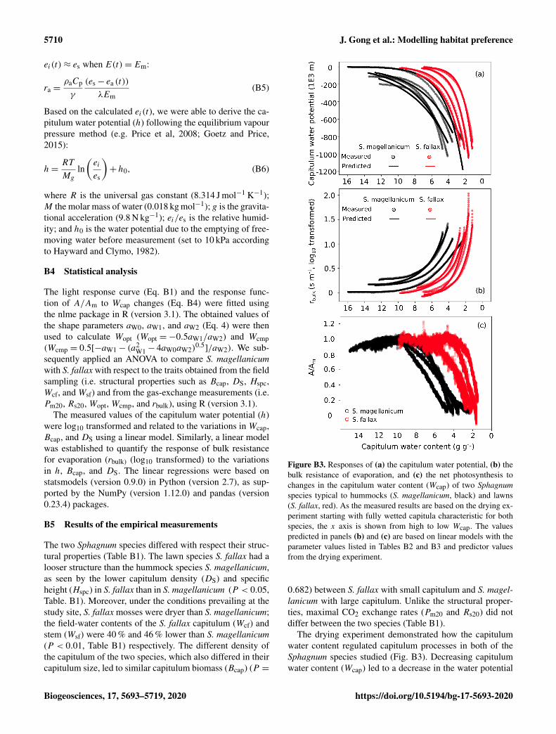
5710 J. Gong et al.: Modelling habitat preference
ei(t)≈ es when E(t)= Em:
ra =ρaCp
γ
(es− ea (t))
λEm(B5)
Based on the calculated ei(t), we were able to derive the ca-pitulum water potential (h) following the equilibrium vapourpressure method (e.g. Price et al, 2008; Goetz and Price,2015):
h=RT
Mg
ln(ei
es
)+h0, (B6)
where R is the universal gas constant (8.314 J mol−1 K−1);M the molar mass of water (0.018 kg mol−1); g is the gravita-tional acceleration (9.8 N kg−1); ei/es is the relative humid-ity; and h0 is the water potential due to the emptying of free-moving water before measurement (set to 10 kPa accordingto Hayward and Clymo, 1982).
B4 Statistical analysis
The light response curve (Eq. B1) and the response func-tion of A/Am to Wcap changes (Eq. B4) were fitted usingthe nlme package in R (version 3.1). The obtained values ofthe shape parameters aW0, aW1, and aW2 (Eq. 4) were thenused to calculate Wopt (Wopt =−0.5aW1/aW2) and Wcmp(Wcmp = 0.5[−aW1− (a
2W1− 4aW0aW2)
0.5]/aW2). We sub-
sequently applied an ANOVA to compare S. magellanicumwith S. fallax with respect to the traits obtained from the fieldsampling (i.e. structural properties such as Bcap, DS, Hspc,Wcf, andWsf) and from the gas-exchange measurements (i.e.Pm20, Rs20, Wopt, Wcmp, and rbulk), using R (version 3.1).
The measured values of the capitulum water potential (h)were log10 transformed and related to the variations in Wcap,Bcap, and DS using a linear model. Similarly, a linear modelwas established to quantify the response of bulk resistancefor evaporation (rbulk) (log10 transformed) to the variationsin h, Bcap, and DS. The linear regressions were based onstatsmodels (version 0.9.0) in Python (version 2.7), as sup-ported by the NumPy (version 1.12.0) and pandas (version0.23.4) packages.
B5 Results of the empirical measurements
The two Sphagnum species differed with respect their struc-tural properties (Table B1). The lawn species S. fallax had alooser structure than the hummock species S. magellanicum,as seen by the lower capitulum density (DS) and specificheight (Hspc) in S. fallax than in S. magellanicum (P < 0.05,Table. B1). Moreover, under the conditions prevailing at thestudy site, S. fallax mosses were dryer than S. magellanicum;the field-water contents of the S. fallax capitulum (Wcf) andstem (Wsf) were 40 % and 46 % lower than S. magellanicum(P < 0.01, Table B1) respectively. The different density ofthe capitulum of the two species, which also differed in theircapitulum size, led to similar capitulum biomass (Bcap) (P =
Figure B3. Responses of (a) the capitulum water potential, (b) thebulk resistance of evaporation, and (c) the net photosynthesis tochanges in the capitulum water content (Wcap) of two Sphagnumspecies typical to hummocks (S. magellanicum, black) and lawns(S. fallax, red). As the measured results are based on the drying ex-periment starting with fully wetted capitula characteristic for bothspecies, the x axis is shown from high to low Wcap. The valuespredicted in panels (b) and (c) are based on linear models with theparameter values listed in Tables B2 and B3 and predictor valuesfrom the drying experiment.
0.682) between S. fallax with small capitulum and S. magel-lanicum with large capitulum. Unlike the structural proper-ties, maximal CO2 exchange rates (Pm20 and Rs20) did notdiffer between the two species (Table B1).
The drying experiment demonstrated how the capitulumwater content regulated capitulum processes in both of theSphagnum species studied (Fig. B3). Decreasing capitulumwater content (Wcap) led to a decrease in the water potential
Biogeosciences, 17, 5693–5719, 2020 https://doi.org/10.5194/bg-17-5693-2020

J. Gong et al.: Modelling habitat preference 5711
Table B1. Species-specific morphological, photosynthetic, and water retention traits from S. magellanicum and S. fallax. Trait values(mean± standard deviation) and ANOVA statistics, F and p values, are given to compare the mean values of traits for the two species.
Trait S. magellanicum S. fallax F P(> F)
Capitulum density, DS (capitula cm−2) 0.922± 0.289 1.46± 0.323 6.224a 0.037∗
Capitulum biomass, Bcap (g m−2) 75.4± 21.5 69.2± 19.6 0.181a 0.682Specific height, Hspc (cm g−1 m−2) 45.4± 7.64 32.6± 6.97 6.126a 0.038∗
Field-water content of capitula, Wcf (g g−1) 14.7± 3.54 8.09± 1.48 11.75a 0.009∗∗
Field-water content of stems, Wsf (g g−1) 18.4± 1.92 10.2± 1.50 45.81a 0.0001∗∗
Maximal gross photosynthesis rate at 20 ◦C, Pm20 (µmol g−1 s−1) 0.019± 0.004 0.014± 0.002 3.737b 0.101Respiration rate at 20 ◦C, Rs20 (µmol g−1 s−1) 0.007± 0.004 0.007± 0.002 0.012b 0.92Half-saturation point of photosynthesis, αPPFD (µmol m−2 s−1) 101.4± 14.1 143± 51.2 2.856b 0.142Optimal capitulum water content for photosynthesis, Wopt (g g−1) 9.41± 0.73 5.81± 1.68 11.57b 0.0145∗
Capitulum water content at the photosynthetic compensation point, Wcmp (g g−1) 3.67± 0.83 1.78± 0.43 12.35b 0.0126∗
Minimal bulk resistance of evaporation, ra (m s−1) 33.5± 7.30 40.7± 4.99 1.976b 0.2165a Soil core measurement, sample n= 5. b Cuvette gas-exchange measurement, sample n= 4. ∗ The difference between the means is significant (P < 0.05). ∗∗ The difference between themeans is very significant (P < 0.01).
Table B2. Parameter estimates of the linear model for the log10-transformed capitulum water potential (h) for S. fallax and S. magellanicum.The estimated value, the standard error (SE), and the test statistics (p values) are given for the predictors of the models. The predictors arethe capitulum biomass (Bcap), the capitulum density (DS), the capitulum water content (Wcap), the interaction of the capitulum biomassand water potential (Bcap×Wcap), the interaction of the capitulum biomass and capitulum density (DS×Wcap), the interaction of thecapitulum density and water potential (DS×Wcap), and the interaction of the capitulum biomass, capitulum density, and water potential(Bcap×DS×Wcap). All coefficient values are significantly different from zero (p < 0.001).
Parameter S. magellanicum (R2= 0.972) S. fallax (R2
= 0.984)
Value SE Value SE
(Intercept) 25.30 0.253 −90.99 2.158Bcap −272.10 3.133 2294.67 52.342Wcap −9.50 0.031 −62.12 0.600Bcap×Wcap 114.61 0.387 1500.26 14.549DS −21.76 0.253 104.11 2.376Bcap×DS 268.95 3.112 −2422.79 55.251DS×Wcap 9.33 0.031 68.35 0.661Bcap×DS×Wcap −113.33 0.386 −1588.06 15.360
Table B3. Parameter estimates of the linear model for the log10-transformed capitulum evaporative resistance (rbulk) for S. fallax andS. magellanicum. The estimated value, the standard error (SE), and the test statistics (p values) are given for the predictors of the models.The predictors are the capitulum biomass (Bcap), the capitulum density (DS), the water potential (h), the interaction of capitulum biomassand water potential (Bcap×h), the interaction of capitulum biomass and capitulum density (DS×h), the interaction of capitulum density andwater potential (DS×h), and the interaction of capitulum biomass, capitulum density, and water potential (Bcap×DS×h). All coefficientvalues are significantly different from zero (p < 0.001).
Parameter S. magellanicum (R2= 0.998) S. fallax (R2
= 0.966)
Value SE Value SE
(Intercept) −1.13 0.027 55.07 2.225Bcap 14.45 0.334 1334.55 53.968h 0.0012 5.92× 10⁻⁵
−0.028 0.004Bcap×h −0.0007 0.001 0.707 0.101DS 1.08 0.027 −60.53 2.450Bcap×DS −13.39 0.333 1406.36 56.968DS×h 0.0002 5.89× 10⁻⁵ 0.0317 0.005Bcap×DS×h −0.0017 0.001 −0.733 0.106
https://doi.org/10.5194/bg-17-5693-2020 Biogeosciences, 17, 5693–5719, 2020

5712 J. Gong et al.: Modelling habitat preference
(h), and the responses of h to Wcap varied among replicates(Fig. 3a). The values of Wcap for S. fallax were generallylower than those for S. magellanicum under the same wa-ter potentials. The fitted linear models explained over 95 %of the variation in the measured h for both species (Ta-ble B2), although the fitted responses of h to Wcap wereslightly smoother than the measured responses, particularlyfor S. magellanicum (Fig. B3a). The responses of h to Wcapwere significantly affected by the capitulum density (DS), thecapitulum biomass (Bcap), and their interactions with Wcap(Table B2).
Decreasing capitulum water content (Wcap) and water po-tential (h) were associated with increasing bulk resistance forevaporation (rbulk, Fig. B3b), although the sensitivity of rbulkto h changes varied by replicate. The values of rbulk fromS. fallax were largely lower than those from S. magellanicumwhen the capitulum water contents of the two species weresimilar. The fitted linear models explained the observed vari-ations in the measured rbulk well for both species (Fig. 2b,Table B3). The variation in the response of rbulkto h was sig-nificantly affected by the capitulum density (DS), the capitu-lum biomass (Bcap), and their interactions with h (Table B3).
Decreasing capitulum water content (Wcap) slowed the netphotosynthesis rate down (Fig. B2c), as represented by thedecreasing ratio of A/Am. S. fallax required a lower capitu-lum water content (Wcap) than S. magellanicum to reach pho-tosynthetic maximum and the photosynthetic compensationpoint. However, the ranges of the capitulum water contentfrom the photosynthetic maximum (Wopt) or field capacity(Wfc) to that at the compensation point (Wcmp) were smallerfor S. fallax than for S. magellanicum. Hence, S. fallax hadnarrower transition zone for photosynthesis to respond todrying compared with S. magellanicum.
Biogeosciences, 17, 5693–5719, 2020 https://doi.org/10.5194/bg-17-5693-2020
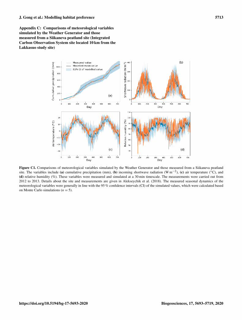
J. Gong et al.: Modelling habitat preference 5713
Appendix C: Comparisons of meteorological variablessimulated by the Weather Generator and thosemeasured from a Siikaneva peatland site (IntegratedCarbon Observation System site located 10 km from theLakkasuo study site)
Figure C1. Comparisons of meteorological variables simulated by the Weather Generator and those measured from a Siikaneva peatlandsite. The variables include (a) cumulative precipitation (mm), (b) incoming shortwave radiation (W m−2), (c) air temperature (◦C), and(d) relative humidity (%). These variables were measured and simulated at a 30 min timescale. The measurements were carried out from2012 to 2013. Details about the site and measurements are given in Alekseychik et al. (2018). The measured seasonal dynamics of themeteorological variables were generally in line with the 95 % confidence intervals (CI) of the simulated values, which were calculated basedon Monte Carlo simulations (n= 5).
https://doi.org/10.5194/bg-17-5693-2020 Biogeosciences, 17, 5693–5719, 2020
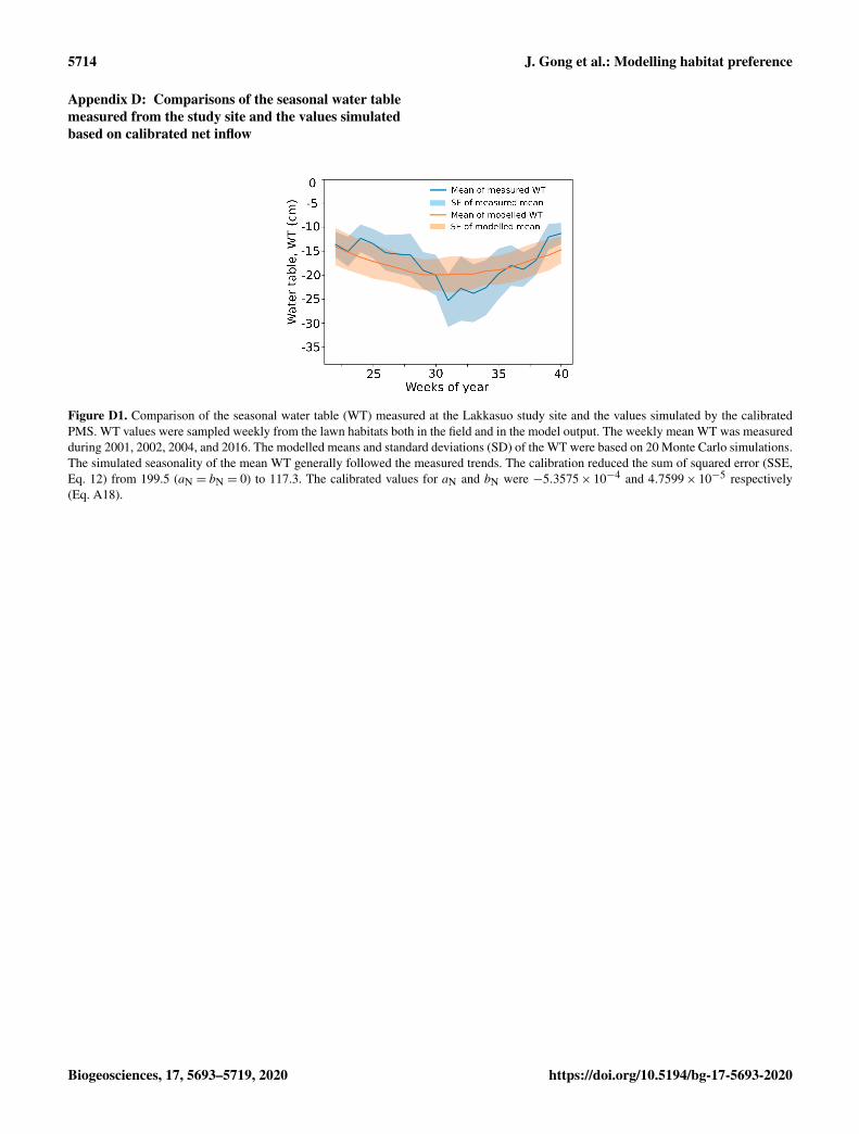
5714 J. Gong et al.: Modelling habitat preference
Appendix D: Comparisons of the seasonal water tablemeasured from the study site and the values simulatedbased on calibrated net inflow
Figure D1. Comparison of the seasonal water table (WT) measured at the Lakkasuo study site and the values simulated by the calibratedPMS. WT values were sampled weekly from the lawn habitats both in the field and in the model output. The weekly mean WT was measuredduring 2001, 2002, 2004, and 2016. The modelled means and standard deviations (SD) of the WT were based on 20 Monte Carlo simulations.The simulated seasonality of the mean WT generally followed the measured trends. The calibration reduced the sum of squared error (SSE,Eq. 12) from 199.5 (aN = bN = 0) to 117.3. The calibrated values for aN and bN were −5.3575× 10⁻⁴ and 4.7599× 10⁻⁵ respectively(Eq. A18).
Biogeosciences, 17, 5693–5719, 2020 https://doi.org/10.5194/bg-17-5693-2020

J. Gong et al.: Modelling habitat preference 5715
Appendix E: List of symbols and abbreviations.
Symbol Description UnitA Net photosynthesis rate (µmol m−2 s−1)Am Maximal net photosynthesis rate (µmol m−2 s−1)αimm Temperature constant for NSC immobilization (–)αPPFD Half-saturation point of PPFD for photosynthesis (µmol m−2 s−1)Bcap Capitulum biomass (g m−2)CT Specific heat (J K−1 kg−1)DS Capitulum density (shoots cm−2)dH Annual vertical growth of Sphagnum mosses (cm)dWT Hummock–lawn differences in the water table (cm)E Rate of evaporation (cm time step−1)fW Water content multiplier on the photosynthesis rate (–)fT Temperature multiplier on the photosynthesis rate (–)h Water potential (cm)Hc Shoot height of Sphagnum mosses (cm)Hcap Height of capitula (cm)Hspc Biomass density of living Sphagnum stems (g m−2 cm−1)I Rate of net inflow water (cm)kimm Specific immobilization rate (g g−1)JDthaw Julian day when thawing completed (–)Kh Hydraulic conductivity of the peat layer (cm s−1)Km Hydraulic conductivity of the moss layer (cm s−1)Ksat Saturated hydraulic conductivity (cm s−1)KT Thermal conductivity (W m−1 K−1)lc Width of a grid cell in the simulation (cm)MB Immobilized NSC to biomass production (g)NSCmax Maximal NSC concentration in Sphagnum biomass (g g−1)P Precipitation (cm)Pm Mass-based rate of maximal gross photosynthesis (µmol g−1 s−1)PPFD Photosynthetic photon flux density (µmol m−2 s−1)ρbulk Bulk density of peat (g cm−3)raero Aerodynamic resistance (s m−1)rbulk Cell-level bulk surface resistance (s m−1)rss Bulk surface resistance of community (s m−1)RH Relative humidity (%)Rs Mass-based respiration rate (µmol g−1 s−1)Rs Incoming shortwave radiation (W m−2)Rl Incoming longwave radiation (W m−2)Sc Area of a cell in the model simulation (m2)simm Multiplier for the temperature threshold (–)Svi Evaporative area of a cell i (cm2)T Capitulum temperature (◦C)Ta Air temperature (◦C)Topt Reference temperature of respiration (20 ◦C) (◦C)u Wind speed (m s−1)Wcap Capitulum water content (g g−1)Wcmp Capitulum water content at the compensation point (g g−1)Wmax Maximum water content of capitula (g g−1)Wopt Optimal capitulum water content for photosynthesis (g g−1)Wcf Field-water contents of the Sphagnum capitulum (g g−1)Wsf Field-water contents of the Sphagnum stem (g g−1)WTm Measured multiyear mean of the weekly water table (cm)WTs Simulated multiyear mean of the weekly water table (cm)zm Thickness of the living moss layer (cm)θm Volumetric water content of the moss layer (–)θr Permanent wilting point water content (–)θs Saturated water content (–)
Abbreviations0 Learning rate of gradient decedent algorithmsD-layer Daily based snow layerICOS Integrated Carbon Observation SystemJD Julian dayNSC Nonstructural carbonPMS Peatland Moss SimulatorRWC Capitulum water contentSD Standard deviationSE Standard errorSSE Sum of squared errorSVAT Soil–vegetation–atmosphere transportWT Water table
https://doi.org/10.5194/bg-17-5693-2020 Biogeosciences, 17, 5693–5719, 2020

5716 J. Gong et al.: Modelling habitat preference
Code and data availability. The data and the code to reproduce theanalysis are available from the corresponding author upon request.
Author contributions. JG and EST designed the study. JG, AML,and NK conducted the experiment and analysis. JG, EST, NR, andSF designed the model. JG coded the model and conducted themodel simulation and data analysis. JG and EST wrote the paperwith contributions from all co-authors.
Competing interests. The authors declare that they have no conflictof interest.
Acknowledgements. The authors are grateful to Harri Strandman(University of Eastern Finland) for coding the Weather Generator.
Financial support. This research has been supported by theAcademy of Finland (project no. 287039), the US National Sci-ence Foundation (grant no. 1802825), the Kone Foundation, and theFulbright-Saastamoinen Foundation.
Review statement. This paper was edited by Michael Bahn and re-viewed by Maaike Bader and two anonymous referees.
References
Alekseychik, P., Lindroth, A., Mammarella, I., Lund, M., Rinne,J., Kasurinen, V., Nilsson, M., Peichl, M., Lohila, A., Aurela,M., Laurila, T., Shurpali, N., Tuittila, E.-S., Martikainen, P.M., and Vesala, T.: Surface energy exchange in natural andmanaged Fennoscandian peatlands, Mires and Peat, 21, 1–26,https://doi.org/10.19189/MaP.2018.OMB.333, 2018.
Alm, J., Shurpali, N. J., Tuittila, E.-S., Laurila, T., Maljanen, M.,Saarnio, S., and Minkkinen, K.: Methods for determining emis-sion factors for the use of peat and peatlands – flux measurementsand modelling, Boreal Environ. Res., 12, 85–100, 2007.
Amarasekare, P.: Competitive coexistence in spatially structured en-vironments: A synthesis, Ecol. Lett., 6, 1109–1122, 2003.
Anderson K. and Neuhauser C.: Patterns in spatial simulations – arethey real?, Ecol. Model., 155, 19–30, 2000.
Andrus R. E.: Some aspects of Sphagnum ecology, Can. J. Bot., 64,416–426, 1986.
Asaeda, T. and Karunaratne, S.: Dynamic modelling of the growthof Phragmites australis: model description, Aquat. Bot., 67, 301–318, 2000.
Bengtsson, F., Granath, G., and Rydin, H.: Photosynthesis, growth,and decay traits in Sphagnum – a multispecies comparison, Ecol.Evol., 6, 3325–3341, 2016.
Blois, J. L., Williams, J. W., Fitzpatrick, M. C., Jackson, S. T., andFerrier, S.: Space can substitute for time in predicting climate-change effects on biodiversity, P. Natl. Acad. Sci. USA, 110,9374–9379, https://doi.org/10.1073/pnas.1220228110, 2013.
Bolker, B. M., Pacala, S. W., and Neuhauser, C.: Spatial dynamics inmodel plant communities: What do we really know?, Am. Nat.,162, 135–148, 2003.
Boulangeat, I., Svenning, J. C., Daufresne, T., Leblond, M., andGravel, D.: The transient response of ecosystems to climatechange is amplified by trophic interactions, Oikos, 127, 1822–1833, 2018.
Branham, J. E. and Strack, M.: Saturated hydraulic conductivityin Sphagnum-dominated peatlands: do microforms matter?, Hy-drol. Process., 28, 4352–4362, 2014.
Chaudhary, N., Miller, P. A., and Smith, B.: ModellingHolocene peatland dynamics with an individual-based dy-namic vegetation model, Biogeosciences, 14, 2571–2596,https://doi.org/10.5194/bg-14-2571-2017, 2017.
Chen, J. M., Liu, J., Cihlar, J., abd Goulden, M. L.: Daily canopyphotosynthesis model through temporal and spatial scaling forremote sensing applications, Ecol. Modell., 124, 99–119, 1999.
Choudhury, B. J. and Monteith, J. L.: A four-layer model for theheat budget of homogeneous land surfaces, Q. J. Roy. Meteor.Soc., 114, 373–398, 1988.
Clapp, R. B. and Hornberger, G. M.: Empirical equations for somesoil hydraulic properties, Water Resour. Res., 14, 601–604, 1978.
Clark, J. S., Bell, D., Chu, C., Courbaud, B., Dietze, M., Hersh,M., HilleRisLambers, J., Ibanez, I., LaDeau, S., McMahon, S.,Metcalf, J., Mohan, J., Moran, E., Pangle, L., Pearson, S., Salk,C., Shen, Z., Valle, D., and Wyckoff, P.: High-dimensional co-existence based on individual variation: a synthesis of evidence,Ecol. Monogr., 80, 569–608, 2010.
Clymo, R. S.: The growth of Sphagnum: Methods of measurement,J. Ecol., 58, 13–49, 1970.
Cornelissen, J. H., Lang, S. I., Soudzilovskaia, N. A., and During,H. J.: Comparative cryptogam ecology: a review of bryophyteand lichen traits that drive biogeochemistry, Ann. Botany, 99,987–1001, 2007
Czárán, T. and Iwasa, Y.: Spatiotemporal models of population andcommunity dynamics, Trends Ecol. Evol., 13, 294–295, 1998.
Daamen, C. C. and McNaughton, K. G.: Modeling energy fluxesfrom sparse canopies and understorys, Agronomy Journal, 92,837–847, 2000.
Dieleman, C. M., Branfireun, B. A., Mclaughlin, J. W., and Lindo,Z.: Climate change drives a shift in peatland ecosystem plantcommunity: Implications for ecosystem function and stability,Glob. Change Biol., 21, 388–395, 2015.
Euskirchen, E. S., Edgar, C. W., Turetsky, M. R., Waldrop, M. P.,and Harden J. W.: Differential response of carbon fluxes to cli-mate in three peatland ecosystems that vary in the presence andstability of permafrost, permafrost, J. Geophys. Res.-Biogeo.,119, 1576–1595, 2014.
Frolking, S., Roulet, N. T., Moore, T. R., Lafleur, T. M., Bubier, L.J., and Crill, P. M.: Modeling seasonal to annual carbon balanceof Mer Bleue Bog, Ontario, Canada, Global Biogeochem. Cy.,16, 4-1-4-21, https://doi.org/10.1029/2001GB001457, 2002.
Gassmann, F., Klötzli, F., and Walther, G.: Simulation of observedtypes of dynamics of plants and plant communities, J. Veg. Sci.,11, 397–408, 2003.
Goetz, J. D. and Price, J. S.: Role of morphological structure andlayering of Sphagnum and Tomenthypnum mosses on moss pro-ductivity and evaporation rates, Can. J. Soil Sci., 95, 109–124,2015.
Biogeosciences, 17, 5693–5719, 2020 https://doi.org/10.5194/bg-17-5693-2020

J. Gong et al.: Modelling habitat preference 5717
Gong, J., Wang, K., Kellomäki, S., Wang, K., Zhang, C., Mar-tikainen, P. J. and Shurpali, N.: Modeling water table changes inboreal peatlands of Finland under changing climate conditions,Ecological Modelling, 244, 65–78, 2012.
Gong, J., Shurpali, N., Kellomäki, S., Wang, K., Salam, M. M., andMartikainen, P. J.: High sensitivity of peat moisture content toseasonal climate in a cutaway peatlandcultivated with a perennialcrop (Phalaris arundinacea, L.): a modeling study, Agr. ForestMeteorol., 180, 225–235, 2013.
Gong, J., Jia, X., Zha, T., Wang, B., Kellomäki, S., and Peltola, H.:Modeling the effects of plant-interspace heterogeneity on water-energy balances in a semiarid ecosystem, Agr. Forest Meteorol.,221, 189–206, 2016.
Gorham, E.: Northern peatlands: Role in the carbon cycle and prob-able responses to climatic warming, Ecol. Appl., 1, 182–195,1991.
Gunnarsson, U., Malmer, N., and Rydin, H.: Dynamics or con-stancy in Sphagnum dominated mire ecosystems?, A 40-yearstudy, Ecography, 25, 685–704, 2002.
Hartmann, H. and Trumbore, S.: Understanding the roles of non-structural carbohydrates in forest trees – from what we can mea-sure to what we want to know, New Phytol., 211, 386–403, 2016.
Hájek, T. and Beckett, R. P.: Effect of water content components ondesiccation and recovery in Sphagnum mosses, Ann. Bot., 101,165–173, 2008.
Hayward P. M. and Clymo R. S.: Profiles of water content and poresize in Sphagnum and peat, and their relation to peat bog ecology,P. Roy. Soc. Lond. B Bio., 215, 299–325, 1982.
Hayward P. M. and Clymo R. S.: The growth of Sphagnum: ex-periments on, and simulation of, some effects of light flux andwater-table depth, J. Ecol., 71, 845–863, 1983.
Holmgren, M., Lin, C., Murillo, J. E., Nieuwenhuis, A., Pen-ninkhof, J., Sanders, N., Bart, T., Veen, H., Vasander, H., Volle-bregt, M. E., and Limpens, J.: Positive shrub-tree interactions fa-cilitate woody encroachment in boreal peatlands, J. Ecol., 103,58–66, 2015.
Hugelius, G., Tarnocai, C., Broll, G., Canadell, J. G., Kuhry, P.,and Swanson, D. K.: The Northern Circumpolar Soil CarbonDatabase: spatially distributed datasets of soil coverage and soilcarbon storage in the northern permafrost regions, Earth Syst.Sci. Data, 5, 3–13, https://doi.org/10.5194/essd-5-3-2013, 2013.
Jassey, V. E. and Signarbieux, C.: Effects of climate warming onSphagnum photosynthesis in peatlands depend on peat moistureand species-specific anatomical traits, Glob. Change Biol., 25,3859–3870, 2019.
Johnson, M. G., Granath, G., Tahvanainen, T., Pouliot, R., Stenøien,H. K., Rochefort, L., Rydin, H., and Shaw, A. J.: Evolution ofniche preference in Sphagnum peat mosses, Evolution, 69, 90–103, 2015.
Kellomäki, S. and Väisänen, H.: Modelling the dynamics of the for-est ecosystem for climate change studies in the boreal conditions,Ecol. Model., 97, 121–140, 1997.
Keuper, F., Dorrepaal, E., Van Bodegom, P. M., Aerts, R., VanLogtestijn, R. S. P., Callaghan, T. V., and Cornelissen, J. H. C.:A Race for Space? How Sphagnum fuscum stabilizes vegeta-tion composition during long-term climate manipulations, Glob.Change Biol., 17, 2162–2171, 2011.
Kokkonen, N., Laine, A., Laine, J., Vasander, H., Kurki, K., Gong,J., and Tuittila, E.-S.: Responses of peatland vegetation to 15-
year water level drawdown as mediated by fertility level. J. Veg.Sci., 30, 1206–1216, 2019.
Korrensalo, A., Hájek, T., Vesala, T., Mehtätalo, L., and Tuittila,E. S.: Variation in photosynthetic properties among bog plants,Botany, 94, 1127–1139, 2016.
Korrensalo, A., Alekseychik, P., Hájek, T., Rinne, J., Vesala, T.,Mehtätalo, L., Mammarella, I., and Tuittila, E.-S.: Species-specific temporal variation in photosynthesis as a moderatorof peatland carbon sequestration, Biogeosciences, 14, 257–269,https://doi.org/10.5194/bg-14-257-2017, 2017.
Kyrkjeeide, M. O., Hassel, K., Flatberg, K. I., Shaw, A. J.,Yousefi, N., and Stenøien, H. K. Spatial genetic struc-ture of the abundant and widespread peatmoss Sphag-num magellanicum Brid, PLoS One, 11, e0148447,https://doi.org/10.1371/journal.pone.0148447, 2016.
Laiho, R.: Decomposition in peatlands: Reconciling seemingly con-trasting results on the impacts of lowered water levels, Soil Biol.Biochem., 38, 2011–2024, 2006.
Laine, A. M. Juurola, E., Hájek, T., and Tuittila, E.-S.: Sphagnumgrowth and ecophysiology during mire succession, Oecologia,167, 1115–1125, 2011.
Laine, J., Komulainen, V.-M., Laiho, R., Minkkinen, K., Rasinmaki,A., Sallantaus, T., Sarkkola, S., Silvan, N., Tolonen, K., Tuittila,E.-S., Vasander, H., and Päivänen, J.: Lakkasuo – a guide to mireecosystem, Department of Forest Ecology Publications, Univer-sity of Helsinki, 31, 123 pp, 2004.
Laine, J., Flatberg, K. I., Harju, P., Timonen, T., Minkkinen, K.,Laine, A., Tuittila, E.-S., and Vasander, H.: Sphagnum Mosses –The Stars of European Mires, University of Helsinki Departmentof Forest Sciences, Sphagna Ky., 326 pp, 2018.
Laine J., Harju P., Timonen T., Laine A., Tuittila E.-S., MinkkinenK., and Vasander H.: The inticate beauty of Sphagnum mosses –a Finnish guide to identification (Univ Helsinki Dept Forest EcolPubl 39), Department of Forest Ecology, University of Helsinki,Helsinki, 1–190, 2009.
Laine, A., Ehonen, S., Juurola, E., Mehtätalo, L., and Tuittila, E.-S.: Performance of late succession species along a chronose-quence: Environment does not exclude Sphagnum fuscum fromthe early stages of mire development, J. Veget. Sci., 26, 291–301,https://doi.org/10.1111/jvs.12231, 2015.
Laing, C. G., Granath, G., Belyea, L. R., Allton K. E., and Ry-din, H.: Tradeoffs and scaling of functional traits in Sphagnumas drivers of carbon cycling in peatlands, Oikos, 123, 817–828,2014.
Larcher, W.: Physiological Plant Ecology: Ecophysiology andStress Physiology of Functional Groups, Springer, 514 pp., 2003.
Letts, M. G., Roulet, N. T., and Comer, N. T.: Parametrizationof peatland hydraulic properties for the Canadian land surfacescheme, Atmos. Ocean, 38, 141–160, 2000.
Martínez-Vilalta, J., Sala, A., Asensio, D., Galiano, L., Hoch,G., Palacio, S., Piper, F. I., and Lloret, F.: Dynamics of non-structural carbohydrates in terrestrial plants: a global synthesis,Ecol. Monogr., 86, 495–516, 2016.
McCarter, C. P. R. and Price, J. S.: Ecohydrology of Sphagnummoss hummocks: mechanisms of capitula water supply and sim-ulated effects of evaporation, Ecohydrology, 7, 33–44, 2014.
Mualem, Y.: A new model for predicting the hydraulic conductivityof unsaturated porous media, Water Resour. Res., 12, 513–522,1976.
https://doi.org/10.5194/bg-17-5693-2020 Biogeosciences, 17, 5693–5719, 2020
5718 J. Gong et al.: Modelling habitat preference
Munir, T. M., Perkins, M., Kaing, E., and Strack, M.: Carbondioxide flux and net primary production of a boreal treedbog: Responses to warming and water-table-lowering simu-lations of climate change, Biogeosciences, 12, 1091–1111,https://doi.org/10.5194/bg-12-1091-2015, 2015.
Murray, K. J., Harley, P. C., Beyers, J., Walz, H., and Tenhunen, J.D.: Water content effects on photosynthetic response of Sphag-num mosses from the foothills of the Philip Smith Mountains,Alaska, Oecologia, 79, 244–250, 1989.
Nijp, J. J., Limpens, J., Metselaar, K., van der Zee, S. E. A. T. M.,Berendse, F., and Robroek, B. J. M.: Can frequent precipitationmoderate the impact of drought on peatmoss carbon uptake innorthern peatlands?, New Phytol., 203, 70–80, 2014.
O’Neill, K. P.: Role of bryophyte-dominated ecosystems in theglobal carbon budget, in: Bryophyte biology, edited by: Shaw, A.J. and Goffi, B., Cambridge University Press, Cambridge, UK,344–368, 2000.
Pastor, J., Peckham, B., Bridgham, S., Weltzin, J., and Chen J.:Plant community dynamics, nutrient cycling, and alternative sta-ble equilibria in peatlands, American Naturalist, 160, 553–568,2002.
Päivänen, J.: Hydraulic conductivity and water retention in peatsoils, Acta Forestalia Fennica, 129, 1–69, 1973.
Price, J. S., Whittington, P. N., Elrick, D. E., Strack, M., Brunet,N., and Faux, E.: A method to determine unsaturated hydraulicconductivity in living and undecomposed moss, Soil Sci. Soc.Am. J., 72, 487–491, 2008.
Price, J. S. and Whittington, P. N.: Water flow in Sphagnum hum-mocks: Mesocosm measurements and modelling, J. Hydrol., 381,333–340, 2010.
Rice, S. K., Aclander, L., and Hanson, D. T.: Do bryophyte shootsystems function like vascular plant leaves or canopies?, Func-tional trait relationships in Sphagnum mosses (Sphagnaceae),Am. J. Botany, 95, 1366–1374, 2008.
Riutta, T., Laine, J., Aurela, M., Rinne, J., Vesala, T., Laurila, T.,Haapanala, S., Pihlatie, M., and Tuittila, E.-S.: Spatial variationin plant community functions regulates carbon gas dynamics ina boreal fen ecosystem, Tellus B, 59, 838–852, 2007.
Robroek, B. J. M., Limpens, J., Breeuwer, A., Crushell, P. H., andSchouten, M. G. C.: Interspecific competition between Sphag-num mosses at different water tables, Funct. Ecol., 21, 805–812,2007a.
Robroek, B. J. M., Limpens, J., Breeuwer, A., van Ruijven, J., andSchouten, M. G. C.: Precipitation determines the persistence ofhollow Sphagnum species on hummocks, Wetlands, 4, 979–986,2007b.
Robroek, B. J. M., Schouten, M. G. C., Limpens, J., Berendse,F., and Poorter, H.: Interactive effects of water table and pre-cipitation on net CO2 assimilation of three co-occurring Sphag-num mosses differing in distribution above the water table, Glob.Change Biol., 15, 680–691, 2009.
Ruder, S.: An overview of gradient descent optimization algorithms,CoRR, abs/1609.04747, 2016.
Runkle, B. R. K., Wille, C., Gažovic, M., Wilmking, M., andKutzbach, L.: The surface energy balance and its drivers in a bo-real peatland fen of northwestern Russia, J. Hydrol., 511, 359–373, 2014.
Rydin, H.: Interspecific competition between Sphagnum mosses ona raised bog, Oikos, 66, 413–423, 1993.
Rydin, H.: Effect of water level on desiccation of Sphagnum in re-lation to surrounding Sphagna, Oikos, 374–379, 1985.
Rydin, H.: Competition and niche separation in Sphagnum, Can. J.Botany, 64, 1817–1824, 1986.
Rydin, H.: Competition between Sphagnum species under con-trolled conditions, Bryologist, 100, 302–307, 1997.
Rydin, H. and McDonald, A. J. S.: Tolerance of Sphagnum to waterlevel, J. Bryol., 13, 571–578, 1985.
Rydin, H., Gunnarsson, U., and Sundberg, S.: The role of Sphag-num in peatland development and persistence, in: Boreal peat-land ecosystems, edited by: Wieder, R. K. and Vitt, D. H., 30Ecological Studies Series, Springer Verlag, Berlin, 47–65, 2006.
Sato, H., Itoh, A., and Kohyama, T.: SEIB-DGVM: A new DynamicGlobal Vegetation Model using a spatially explicit individual-based approach, Ecol. Model., 200, 279–307, 2007.
Scheiter, S., Langan, L., and Higgins, S. I.: Next-generation dy-namic global vegetation models: learning from community ecol-ogy, New Phytol., 198, 957–969, 2013.
Schipperges, B. and Rydin, H.: Response of photosynthesis ofSphagnum species from contrasting microhabitats to tissue wa-ter content and repeated desiccation, New Phytol., 140, 677–684,1998.
Smirnoff, N.: The carbohydrates of bryophytes in relation to desic-cation tolerance, J. Bryology, 17, 185–191, 1992.
Straková, P., Niemi, R. M., Freeman, C., Peltoniemi, K., Toberman,H., Heiskanen, I., Fritze, H., and Laiho, R.: Litter type affects theactivity of aerobic decomposers in a boreal peatland more thansite nutrient and water table regimes, Biogeosciences, 8, 2741–2755, https://doi.org/10.5194/bg-8-2741-2011, 2011.
Straková, P., Penttilä, T., Laine, J., and Laiho, R.: Disentangling di-rect and indirect effects of water table drawdown on above-andbelowground plant litter decomposition: consequences for accu-mulation of organic matter in boreal peatlands, Glob. ChangeBiol., 18, 322–335, 2012.
Strandman, H., Väisänen, H., and Kellomäki, S.: A procedure forgenerating synthetic weather records in conjunction of climaticscenario for modelling of ecological impacts of changing climatein boreal conditions, Ecol. Model., 70, 195–220, 1993.
Tahvanainen, T.: Abrupt ombrotrophication of a boreal aapa miretriggered by hydrological disturbance in the catchment, J. Ecol.,99, 404–415, 2011.
Tatsumi, S., Cadotte M. W., and Mori, A. S.: Individual-based mod-els of community assembly: Neighbourhood competition drivesphylogenetic community structure, J. Ecol., 107, 735–746, 2019.
Thompson, D. K., Baisley, A. S., and Waddington, J. M.: Seasonalvariation in albedo and radiation exchange between a burned andunburned forested peatland: implications for peatland evapora-tion, Hydrol. Proc., 29, 3227–3235, 2015.
Titus, J. E. and Wagner, D. J.: Carbon balance for two Sphagnummosses: water balance resolves a physiological paradox, Ecol-ogy, 65, 1765–1774, 1984.
Turetsky, M. R.: The role of bryophytes in carbon and nitrogen cy-cling, Bryologist, 106, 395–409, 2003.
Turetsky, M. R., Crow, S. E., Evans, R. J., Vitt, D. H., and Wieder,R. K.: Trade-offs in resource allocation among moss species con-trol decomposition in boreal peatlands, J. Ecol., 96, 1297–1305,2008.
Turetsky, M. R., Bond-Lamberty, B., Euskirchen, E., Talbot, J.,Frolking, S., McGuire, A. D., and Tuittila, E.: The resilience
Biogeosciences, 17, 5693–5719, 2020 https://doi.org/10.5194/bg-17-5693-2020

J. Gong et al.: Modelling habitat preference 5719
and functional role of moss in boreal and arctic ecosystems, NewPhytol., 196, 49–67, 2012.
van Gaalen, K. E., Flanagan, L. B., Peddle, D. R.: Photosynthesis,chlorophyll fluorescence and spectral reflectance in Sphagnummoss at varying water contents, Oecologia, 153, 19–28, 2007.
van Genuchten, M.: A closed-form equation for predicting the hy-draulic conductivity of unsaturated soils, Soil Sci. Soc. Am. J.,44, 892–898, 1980.
Väliranta, M., Korhola, A., Seppä, H., Tuittila, E. S., Sarmaja-Korjonen, K., Laine, J., and Alm, J.: High-resolution recon-struction of wetness dynamics in a southern boreal raised bog,Finland, during the late Holocene: a quantitative approach,Holocene, 17, 1093–1107, 2007.
Venäläinen, A., Tuomenvirta, H., Lahtinen, R., and Heikinheimo,M.: The influence of climate warming on soil frost on snow-freesurfaces in Finland, Climate Change, 50, 111–128, 2001.
Vionnet, V., Brun, E., Morin, S., Boone, A., Faroux, S., LeMoigne, P., Martin, E., and Willemet, J.-M.: The detailed snow-pack scheme Crocus and its implementation in SURFEX v7.2,Geosci. Model Dev., 5, 773–791, https://doi.org/10.5194/gmd-5-773-2012, 2012.
Vitt, D. H.: Peatlands: Ecosystems dominated by bryophytes, in:Bryophyte biology, edited by: Shaw, A. J. and Goffi, B., Cam-bridge University Press, Cambridge, UK, 312–343, 2000.
Waddington, J. M., Morris, P. J., Kettridge, N., Granath, G., Thomp-son, D. K., and Moore, P. A.: Hydrological feedbacks in northernpeatlands, Ecohydrology, 8, 113–127, 2015.
Wania, R., Ross, I., and Prentice, I. C.: Integrating peat-lands and permafrost into a dynamic global vegetationmodel: 2. Evaluation and sensitivity of vegetation and car-bon cycle processes, Global Biogeochem. Cy., 23, GB3015,https://doi.org/10.1029/2008GB003413, 2009.
Weiss, R., Alm, J., Laiho, R., and Laine, J.: Modeling moisture re-tention in peat soils, Soil Sci. Soc. Am. J., 62, 305–313, 1998.
Whittington, P. N. and Price, J. S.: The effects of water table draw-down (as a surrogate for climate change) on the hydrology of afen peatland, Canada, Hydrol. Proc., 20, 3589–3600, 2006.
Wilson, P. G.: The relationship among micro-topographic varia-tion, water table depth and biogeochemistry in an ombrotrophicbog, Master Thesis, Department of Geography McGill Univer-sity, Montreal, Quebec, p. 103, 2012.
Wojtun, B., Sendyk, A., and Martynia, D.: Sphagnum species alongenvironmental gradients in mires of the Sudety Mountains (SWPoland), Boreal Environ. Res., 18, 74–88, 2003.
Wu, J. and Roulet, N. T.: Climate change reduces the capacity ofnorthern peatlands to absorb the atmospheric carbon dioxide:The different responses of bogs and fens, Global Biogeochem.Cy., 28, 1005–1024, https://doi.org/10.1002/2014GB004845,2014.
Wullschleger, S. D., Epstein, H. E., Box, E. O., Euskirchen, E. S.,Goswami, S., Iversen, C. M., Kattge, J., Norby, R. J., van Bode-gom, P. M., and Xu, X.: Plant functional types in Earth systemmodels: past experiences and future directions for applicationof dynamic vegetation models in high-latitude ecosystems, Ann.Bot., 114, 1–16, 2014.
https://doi.org/10.5194/bg-17-5693-2020 Biogeosciences, 17, 5693–5719, 2020
Copyright © 2022 FDOKUMEN