The Dissolution of the Family. A Consequence of Misinterpretation?
Upload
khangminh22Category
view
0download
0
Modelling Dissolution of Precipitate Phases During
Homogenization of Aluminum Alloy B319
by
Ida Sadeghi
A thesis
presented to the University of Waterloo
in fulfilment of the
thesis requirement for the degree of
Master of Applied Science
in
Mechanical Engineering
Waterloo, Ontario, Canada, 2016
© Ida Sadeghi 2016

ii
Author's Declaration
I hereby declare that I am the sole author of this thesis. This is a true copy of the thesis,
including any required final revisions, as accepted by my examiners. I understand that my thesis
may be made electronically available to the public.

iii
Abstract
Increasing the knowledge about the heat treatment of Aluminum alloys as light metals
can be useful since these alloys are used in automotive industry, and optimizing their heat
treatment processes can be beneficial economically. Aluminum B319 which is of the type Al-Si-
Cu-Mg was used in this study. The result of a theoretical study of diffusion-controlled
dissolution of planar, cylindrical, spherical and elliptical θ-Al2Cu precipitates are presented.
Graphical relationships between the precipitate size and dissolution time were developed for a
constant diffusion coefficient. The validity of various approximate solutions including: stationary
interface, moving boundary using MATLAB and moving boundary using COMSOL software
were considered. COMSOL was capable of two-dimensional and three-dimensional modelling.
In addition, the dissolution of the Q-Al5Mg8Si6Cu2 precipitate which is a multi-component phase
— that involves the diffusion of more than one component during the dissolution process — as
well as the concurrent dissolution of θ-Al2Cu and Q-Al5Mg8Si6Cu2 were modelled using
MATLAB. Both two and three-dimensional models were developed using COMSOL. Numerical
models were validated through a series of experimental measurements using a fluidized bath
furnace. The results show that the model predictions are in good agreement with the
experimental results and little variations are due to the simplifications made in the model. The
effect of Secondary Dendrite Arm Spacing (SDAS) on dissolution time was also examined and it
was shown that the model developed was able to accurately capture these effects as well on the
time required for dissolution to of these phases to occur. The model can be used as a tool to
identify potential optimisation strategies for industrial solution heat treatment processes.
Key words: Solution heat treatment; Homogenization; Al B319; θ phase; Q phase;
Modelling; COMSOL; MATLAB; SDAS.

iv
Acknowledgments
I would like to express my sincere gratitude to Professor Mary A. Wells for her
immeasurable supports; whom without her supports, this project could not have been as a
memorable learning experience as it has been. I would also like to thank Professor Shahrzad
Esmaeili for co-supervising me and always giving me beneficial advice that helped me a great
deal throughout the project. I would like to thank my two supervisors for not only being
supportive professionally, but also spiritually during these years I have been working with them.
I would also like to thank all the people in the Mechanical and Mechatronics Engineering
department who helped me during this project. Specifically, thanks is given to Yuquan Ding,
SEM lab advisor, for helping me with scanning electron microscope and for always offering
useful advice. I would also like to thank Richard Gordon for being one of the best people in the
world who with his thoughtfulness always made the lab a more enjoyable place to be in. I would
also like to thank the technicians at the student shop especially Phil Laycock for teaching me
how to use the machinery.
Finally, I would like to acknowledge the financial assistance I received from Auto21 and
University of Waterloo.

v
Table of Content
Author's Declaration ....................................................................................................................... ii Abstract .......................................................................................................................................... iii Acknowledgments.......................................................................................................................... iv Table of Content ............................................................................................................................. v
List of Figures ............................................................................................................................... vii List of Tables .................................................................................................................................. x
List of Abbreviations ..................................................................................................................... xi List of Symbols ............................................................................................................................. xii
1. Introduction ............................................................................................................................. 1 2. Background .............................................................................................................................. 3
2.1 Cast AlB319 alloys..................................................................................................................................... 3
2.2 Heat treatment of AlB319 alloys ......................................................................................................... 5 2.2.1 Solution treatment .......................................................................................................... 5 2.2.2 Quenching ..................................................................................................................... 10
2.2.3 Aging ............................................................................................................................ 11
2.3 Modelling dissolution during homogenization ........................................................................... 13 3. Scope and objectives ............................................................................................................. 20
4. Modelling and Experimental Methods .................................................................................. 22
4.1 Model development ............................................................................................................................... 23 4.1.1 Model assumptions ....................................................................................................... 23 4.1.2 Description of the Models ............................................................................................ 24
4.1.3 Fixed mesh approach .................................................................................................... 25 4.1.3.1 Governing equati .................................................................................................... 26 4.1.3.2 Initial conditions .................................................................................................... 29
4.1.3.3 Boundary conditions .............................................................................................. 30 4.1.4 Moving mesh ................................................................................................................ 31
4.1.4.1 Governing equations .............................................................................................. 31 4.1.4.2 Boundary conditions .............................................................................................. 33 4.1.4.3 Model consistency assessment ............................................................................... 34
4.1.5 COMSOL ..................................................................................................................... 34
4.2 Morphology analysis ............................................................................................................................. 36 4.2.1 COMSOL ..................................................................................................................... 36 4.2.2 MATLAB ..................................................................................................................... 36
4.3 Thermodynamic analysis .................................................................................................................... 37
4.4 Segregation analysis .............................................................................................................................. 41
4.5 Experiments ............................................................................................................................................. 43 4.5.1 Wedge casing ................................................................................................................ 43
4.5.2 Chemical composition .................................................................................................. 43

vi
4.5.3 Heat Treatment ............................................................................................................. 44
4.5.4 Metallography and Image Analysis .............................................................................. 45 5. Results and Discussion .......................................................................................................... 46
5.1 Microstructural investigations .......................................................................................................... 46
5.2 Model predictions and experimental results ............................................................................... 50 5.2.1 Conventional furnace versus fluidized bed .................................................................. 50 5.2.2 Mesh sensitivity ............................................................................................................ 51
5.2.3 Single component fixed mesh model -MATLAB ........................................................ 53 5.2.4 Multi-component moving mesh model -MATLAB ..................................................... 55 5.2.5 Q-phase dissolution ...................................................................................................... 57 5.2.6 COMSOL ..................................................................................................................... 60 5.2.7 Effect of particle morphology....................................................................................... 63
5.2.8 Effect of the diffusion field size on the particle dissolution ......................................... 68
5.2.9 Homogenization ........................................................................................................... 69
6. Conclusions and Future work ................................................................................................ 72
6.1 Conclusions ............................................................................................................................................... 72
6.2 Future work .............................................................................................................................................. 73 7. References ............................................................................................................................. 75 Appendices .................................................................................................................................... 82

vii
List of Figures
Figure 2.1: A typical as-cast microstructure of Al-Cu-Si-Mg alloys; 1) Aluminum matrix, 2) Si
eutectic, 3) Iron intermetallic and 4) Al2Cu phase [13]. ................................................................. 4
Figure 2.2: Typical phases present in the Al-Si-Cu-Mg alloys; a) Si eutectic and b) skeleton-like
Al15(FeMn)3Si2 phase and c) Al2Cu eutectic; deep etched in HCl [10]. ......................................... 4
Figure 2.3: General schematic presentation of primary and secondary dendrite arm spacings
(PDAS and SDAS) [6]. ................................................................................................................... 4
Figure 2.4: A schematic presentation of the dissolution of a) eutectic and b) blocky Al2Cu
[26,27] ............................................................................................................................................. 7
Figure 2.5: A schematic presentation of eutectic binary phase diagram [15]. ................................ 8
Figure 2.6: T6 heat treatment of Al-Si-Cu alloys [5]. ................................................................... 12
Figure 2.7: Dissolution times for planar, spherical and cylindrical precipitates as a function of
saturation, CA [52]. ....................................................................................................................... 16
Figure 2.8: The interface position as a function of time during the dissolution of a planar phase
obtained for analytical and numerical solutions [60]. ................................................................... 18
Figure 4.1: A schematic presentation of the steps involved in the particle dissolution process. .. 23
Figure 4.2: A schematic presentation of stationary interface dissolution process for a spherical
particle........................................................................................................................................... 26
Figure 4.3: A schematic of secondary phase particles location and the diffusion field around the
particle........................................................................................................................................... 26
Figure 4.4: The diffusion field around particle and the diffusion shells. ...................................... 28
Figure 4.5: A schematic presentation of the situation in which particle growth occurs instead of
dissolution. .................................................................................................................................... 30
Figure 4.6: A schematic presentation of the Concentration profile in the matrix around particle as
dissolution time elapses. ............................................................................................................... 30
Figure 4.7: A schematic of moving interface dissolution process. ............................................... 31
Figure 4.8: Mesh used in COMSOL. ............................................................................................ 35
Figure 4.9: Phase diagram of AlB319........................................................................................... 38
Figure 4.10: Phase stability in AlB319 at different temperatures. ................................................ 39
Figure 4.11: Calculated diffusion coefficients of the impurities Mg, Si and Cu in Al in
comparison with Al self-diffusion [75]......................................................................................... 39
Figure 4.12: Density of Al-Si alloys at different a) Cu and b) Si content [80]. ............................ 40
Figure 4.13: Schematic of the cast ingot showing the different sections’ microstructure (distances
are in mm). .................................................................................................................................... 44
Figure 5.1: As-cast microstructure showing dendritic microstructure and different phases at a).
smaller and b) larger magnification. ............................................................................................. 47
Figure 5.2: Optical micrograph of the as-cast at SDAS of a) 14 and (b) 22 µm. ......................... 48
Figure 5.3: a) The morphologies of iron-intermetallic phases and b) nucleation of precipitates on
Fe-intermetallic. ............................................................................................................................ 49

viii
Figure 5.4: a) The θ and Q phases and b) different types of the θ phase. ..................................... 49
Figure 5.5: a) as-cast and solution heat treated for 8 hrs at 500 °C for SDAS of b) 14 µm and c)
22 µm. ........................................................................................................................................... 50
Figure 5.6: Experimentally measured volume fraction of Al2Cu particle vs. dissolution time for
Conventional Furnace (CF) and Fluidized Bed (FB). ................................................................... 51
Figure 5.7: Mesh sensitivity of the SCFM approximate for different number of meshes. ........... 52
Figure 5.8: Mesh sensitivity of the MCMM approximate for different number of meshes. ........ 52
Figure 5.9: Mesh sensitivity of COMSOL approximate at different mesh sizes. ......................... 53
Figure 5.10: Experimental measurements (symbols) versus SCFM approach model predictions
(lines). ........................................................................................................................................... 54
Figure 5.11: Experimental measurements (symbols) versus MCMM approach model predictions
(lines). ........................................................................................................................................... 55
Figure 5.12: Experimental measurements (symbols) versus MCMM approach model predictions
(lines). ........................................................................................................................................... 56
Figure 5.13: Dissolution of the Q phase. ...................................................................................... 58
Figure 5.14: Concentration of Cu within the diffusion field at different times of heat treatment. 59
Figure 5.15: Concentration of Mg in the diffusion field at different times of heat treatment. ..... 59
Figure 5.16: Concentration of Si in the diffusion field at different times of heat treatment. ....... 59
Figure 5.17: Experimental measurements (symbols) versus 2D COMSOL predictions (lines) for
a spherical particle. ....................................................................................................................... 60
Figure 5.18: Experimental measurements (symbols) versus 2D COMSOL predictions (lines) for
ellipsoid particle with aspect ratio of 8. ........................................................................................ 61
Figure 5.19: Experimental measurements (symbols) versus 3D COMSOL predictions (lines) for
a spherical particle. ....................................................................................................................... 61
Figure 5.20: Experimental measurements (symbols) versus 3D COMSOL predictions (lines) for
ellipsoid particle with aspect ratio of 5. ........................................................................................ 62
Figure 5.21: Experimental measurements (symbols) versus 3D COMSOL predictions (lines) for
ellipsoid particle with aspect ratio of 7. ........................................................................................ 62
Figure 5.22: COMSOL predictions and experimental results in two step solution heat treatment.
Figure 5.23: MCMM prediction of the effect of particle shape on the dissolution time. ............. 64
Figure 5.24: COMSOL predictions of the dissolution of an elliptical particle with different aspect
ratios. ............................................................................................................................................. 65
Figure 5.25: COMSOL predictions of the effect of particle shape on the dissolution time. ........ 65
Figure 5.26: COMCOL prediction of the concentration Cu within the diffusion filed and radius
of a spherical particle versus time for a 2D Circle (SDAS=22 µm, temperature= 500 °C) at (a) 0,
(b) 500, (c) 1500 and (d) 2100 sec. ............................................................................................... 66
Figure 5.27: COMCOL prediction of the concentration of Cu within the diffusion field and
radius of a planar particle versus time for a 2D Circle (SDAS=22 µm, temperature= 500 °C) at
(a) 0, (b) 500, (c) 1500 and (d) 2100 sec. ..................................................................................... 67
Figure 5.28: COMCOL prediction of the concentration of Cu within the diffusion field and
radius of an elliptical particle versus time for a 2D Circle (SDAS=22 µm, temperature= 500 °C)
at (a) 0, (b) 500, (c) 1500 and (d) 2100 sec................................................................................... 68
Figure 5.29: Dissolution time for a spherical particle at different diffusion field sizes. .............. 69
Figure 5.30: Dissolution time for a planar particle at different diffusion field sizes. ................... 69
Figure 5.31: Dissolution and homogenization times for different SDASs at T = 500 °C. ........... 70

ix
Figure 5.32: Concentration gradient along the diffusion field at T = 500 °C and for SDAS of 22
μm. ................................................................................................................................................ 71
Figure B.1: Thermocalc predictions for AlB319 phase diagram. ................................................. 85
Figure C.1: FactSage prediction for phase diagram of AlB319.................................................... 86
Figure D.1: The interfacial position as a function of time for a planar dissolving particle; a)
Vermolen model and b) model of this study. ................................................................................ 87
Figure D.2: The interfacial position as a function of time for a planar dissolving particle; a)
Vermolen model and b) model of this study. ................................................................................ 88
Figure D.3: The interfacial position as a function of time for a spherical dissolving particle; a)
Vermolen model and b) model of this study. ................................................................................ 88

x
List of Tables
Table 1.1: Reactions occurring during solidification of 319.1 alloy at 0.6 °C/s [14]. .................... 5
Table 2.1: Model predictions for A356 and A357 [54]. ............................................................... 17
Table 4.1: COMSOL mesh quantification. ................................................................................... 35
Table 4.2: Enthalpies, entropies and solubility products of the θ and Q phases. .......................... 40
Table 4.3: 319 chemical composition. .......................................................................................... 43
Table 5.1: As-cast microstructure parameters. ............................................................................. 46
Table D.1: Input data. ................................................................................................................... 87

xi
List of Abbreviations
PDAS Single Component Fixed Mesh
SDAS Secondary Dendrite Arm Spacing
SEM Scanning Electron Microscope
SE Secondary Electron
OM Optical Microscope
EPMA Electron Probe Micro Analysis
CF Conventional Furnace
FB Fluidized Bath
SCFM Single Component Fixed Mesh
MCMM Multi Component Moving Mesh
UDF User Defined Function
1D One Dimensional
2D Two Dimensional
3D Three Dimensional
xii
List of Symbols
θ Al2Cu phase
Q Al5Mg8Si6Cu2 phase
A Area [m2]
J Diffusion flux [mol/m2.s]
D Diffusion coefficient [m2/s]
𝐷0 Diffusivity factor [m2/s]
𝑘𝑖 Partition coefficient
𝐾𝑠𝑜𝑙 Solubility product [mol/L]
𝐾0 Pre-exponential factor for solubility [mol/L]
∆𝐻 Enthalpy of formation [kJ]
∆𝑆 Entropy of formation [J/K]
𝐶𝐼 Solute concentration at the particle-matrix interface [wt%]
𝐶𝑀 Solute concentration in the matrix [wt%]
𝐶𝑃 Solute concentration within the particle [wt%]
𝑐𝑖𝑝𝑎𝑟𝑡
Concentration of diffusing element in the particle[wt%]
𝑐𝑖𝑠𝑜𝑙 Concentration of element 𝑖 at the particle-matrix interface[wt%]
𝐶𝐴𝑙𝑙𝑜𝑦 Concentration of the solute in the alloy[wt%]
𝐶𝑀𝐶𝑢, 𝐶𝑀
𝑆𝑖, 𝐶𝑀𝑀𝑔
Concentration of Cu, Si and Mg in the matrix[wt%]
𝑐𝐶𝑢𝑄
, 𝑐𝑆𝑖𝑄
, 𝑐𝑀𝑔𝑄
Concentration of Cu, Si and Mg within the Q phase[wt%]
𝑟𝑑𝑓 Radius of the diffusion field [m]
𝑟0 Initial radius of the spherical particle [m]
𝑓𝑣𝑝 Volume fraction of the particles
𝑓𝑣𝐴𝑙𝑙𝑜𝑦
Volume fraction of the alloy
𝑓𝑣𝑀𝑎𝑡𝑟𝑖𝑥 Volume fraction of the matrix

xiii
𝜌𝐴𝑙𝑙𝑜𝑦 Density of the alloy [g/cm3]
𝜌𝑄 Density of the Q phase [g/cm3]
𝜌𝜃 Density of the θ phase [g/cm3]
𝑓 Fraction of solid phase
∆𝑇 Temperature gradient [K]
𝜆𝑑𝑒𝑛 Dendrite arm spacing [m]
S Segregation ratio

1
Chapter 1
1. Introduction
Aluminum is the most heavily consumed non-ferrous metal in the world, with current
annual consumption at 24 million tons [1]. The demand for improved fuel efficiency in
automobiles without impairing performance has led to an increased use of aluminum alloys in
the production of a wide variety of castings such as engine blocks, cylinder heads and manifolds
(Fig. 1.1). Aluminum casting offers the important advantage of being able to produce lightweight
and highly complex functional shapes quickly and easily. Cost is reduced because numerous
parts and complex construction and processing steps can be replaced by a single cast part [2].
Aluminum casting alloys such as the type Al-Si-Cu-Mg are hypoeutectic and are normally
produced from scrap metal. Al B319 is a type of Al-Si-Cu-Mg alloy with 5.5-6.5 % Si, 3-4 % Cu
and <0.5 % Mg. The microstructure expected in a casting made from this alloy will be a mixture
of pre-eutectic aluminium dendrites surrounded by Al–Si eutectic, and various types of Cu phase
precipitates. The presence of tramp elements from the scrap promotes the formation of various
other phases. For example, iron promotes the formation of various intermetallic phases, the most
common of which are Al5FeSi and Al15(Mn,Fe)3Si2. Mg, added to strengthen aluminium alloys
by precipitation of Mg2Si particles, should be limited to narrow margins in castings hardened by
precipitation of Al2Cu, as in the case of B319, as it tends to form a low melting point eutectic
(Al-Si-Al5Mg8Cu2Si6) that solidifies at temperatures below 500°C [3-5].
The mechanical properties of a casting are controlled by its microstructure which, in turn,
is influenced by the chemical composition of the alloy, i.e., by its Si, Mg, and Cu content, and by
the presence of impurities such as iron, and casting defects (porosity, inclusions, etc.), as well as
the solidification history (i.e., cooling rate) and subsequent heat treatment [2]. In the case of
A319 alloys, this would imply the α-Al dendrite arm spacing (DAS), the morphology and size of
the eutectic Si particles, and the amount of intermetallics and/or other second-phase constituents
present in the microstructure; all play a role in final mechanical properties. Cooling rate controls

2
the fineness of the as-cast microstructure; by increasing the cooling rate, microstructure is
characterized by finer eutectic Si particles, finer α-Al dendrites and other phase particles, and
smaller dendrite arm spacing, while by increasing the solidification time the formation of a
coarse Si particles is predominant [6].
Castings are inhomogeneous due to microsegregation and macrosegregation. Uniform
distribution of the solute elements is very important as it plays a vital role in the subsequent
thermomechanical processing of the alloy. Heat treatments such as solutionizing, quenching and
aging are applied to homogenize microstructure and ameliorate its mechanical properties.
The production of aluminum engine component castings is in many cases a multi-step
manufacturing process, where the casting will pass a heat treatment process after its
solidification. Figure 1.2 schematically describes the most important manufacturing steps [8].
Figure 1.1: Production cycle of aluminum B319.
Time
1
2
3
4
Casting
Building up stresses and distortions
Casting
Building up distortion and relieving stresses
Casting
Distortion, building up stresses again
Casting
Stress relaxation but not stress free, distortion 1
2
3
4
Casting
Solutionizing
Quenching
Aging
Temperature

3
Chapter 2
2. Background
2.1 Cast AlB319 alloys
Aluminum B319 alloy is of type Al-Si-Cu-Mg alloys. The main phases in the as-cast
AlB319 are dendritic α-Al, Al-Si eutectic phase and θ (Al2Cu) precipitates although Mg, Fe, Mn
and other intermetallics are present to some extent [9] (Fig. 2.1). At higher Mg concentrations Q
(Al5Mg8Cu2Si6) and β (Mg2Si) phases also precipitate out (shown in Figure 2.1 – which points).
The eutectic Si is in the form of brittle acicular plates that are detrimental to the tensile and
impact properties [2]. Iron intermetallic first precipitates as Al15(FeMn)3Si2 phase that is in the
form of skeleton-like or Chinese-script which does not initiate cracks to the same extent as the
Al5FeSi particles which are in the form of long platelets. The Al5FeSi phase is detrimental to
mechanical properties especially ductility, and can also cause shrinkage porosity in castings [10].
Al2Cu phase precipitates in two distinct forms, i.e., block-like (coarse Al2Cu precipitates) and
eutectic-like (fine Al2Cu particles interspersed with Al) (Figure 2.2). The proportion of the
block-like form increases with decreasing solidification rate, increasing volume fraction of β-
Al5FeSi needles, and modification of the alloy with strontium. The increased number of modified
silicon particles serves as nucleation sites for precipitation of very fine individual Al2Cu particles
[11]. Eutectic Al-Al2Cu-Si forms on Si, β needles, block-like Al2Cu or as separate pockets within
Al matrix [12].
The cooling rate during solidification affects the eutectic silicon size and secondary
dendrite arm spacing. Primary and secondary dendrite arm spacings are shown in Figure 2.3.
Sand castings solidify at an average solidification rate of lower than 5 °C/s [13].

4
Figure 2.1: A typical as-cast microstructure of Al-Cu-Si-Mg alloys; 1) Aluminum matrix, 2) Si eutectic,
3) Iron intermetallic and 4) Al2Cu phase [13].
Figure 2.2: Typical phases present in the Al-Si-Cu-Mg alloys; a) Si eutectic and b) skeleton-like
Al15(FeMn)3Si2 phase and c) Al2Cu eutectic; deep etched in HCl [10].
Figure 2.3: General schematic presentation of primary and secondary dendrite arm spacings (PDAS and
SDAS) [6].
SDAS
(a) (b)
PDAS
(c)

5
The solidification sequence in 319.1alloy is reported by Backerud et al. [14] and listed in
Table 1.1.
Table 1.1: Reactions occurring during solidification of 319.1 alloy at 0.6 °C/s [14].
Reaction Suggested Temperature (°C)
1. Development of α-aluminum dendrite network 609
2a. Liquid Al + Al15Mn3Si2 590
2b. Liquid Al + Al5FeSi + Al15Mn3Si2 590
3. Liquid Al + Si + Al5FeSi 575
4. Liquid Al + Al2Cu + Si + Al5FeSi 525
5. Liquid Al + Al2Cu + Si + Al5Mg8Cu2Si6 507
2.2 Heat treatment of AlB319 alloys
Homogenization is a common industrial practice after solidification to obtain the required
casting properties. It is a diffusion-controlled process, and its kinetics depends on several factors,
such as temperature, diffusion distance (i.e. secondary dendrite arm spacing), diffusivity of the
solutes, dissolution rate, and so on. Usually it is carried out on castings to improve the properties
of the casting or to facilitate the subsequent steps in the processing to final products [2,15].
Homogenization literally refers to equalization of solute concentration in the single phase
(or removing segregation), however, solution heat treatment refers to the process which is mainly
related to the secondary phase particle dissolution into the matrix [2,16]. Heat treatment done on
AlB319 consists of solution heat treatment, quenching and then aging.
2.2.1 Solution treatment
Solution heat treatment must be applied for a sufficient length of time to obtain a
homogeneous supersaturated structure, followed by quenching with the aim of maintaining the

6
supersaturated structure at ambient temperature. In Al-Si-Cu-Mg alloys, the solution treatment
fulfils three roles:
i. Homogenization of the as-cast structure.
ii. Dissolution of certain intermetallic phases such as Al2Cu and Mg2Si.
iii. Spheroidization of eutectic silicon [2,17,18].
The segregation of solute elements resulting from dendritic solidification may have an adverse
effect on mechanical properties. The time required for homogenization is determined by the
solution temperature and by the dendrite arm spacing [19]. Hardening alloying elements such as
Cu and Mg display significant solid solubility in heat-treatable aluminum alloys at the solidus
temperature; this solubility decreases noticeably as the temperature decreases.
Time and temperature for solutionizing should be optimized. Too long solution treatment
at low temperature causes secondary porosity formation during annealing, coarsening of the
microstructural constituents and increased processing costs, while too short solutionizing does
not lead to a complete dissolution of the alloying elements responsible for subsequent
precipitation hardening. From another point, low solution treatment temperature will not
homogenize the microstructure, however, high solutionizing temperature can lead to incipient
melting and formation of structureless phases when quenching, and storage of high thermal stress
in the alloy due to quenching from higher temperature [18,20]. The smaller the SDAS the lower
the time needed for solutionizing. Melting of Cu-containing phases starts at lower temperatures
as the Mg-content of the alloy increases. Hence, the choice of optimum solution treatment
temperature depends on Cu and Mg content of the alloy. The higher the solution treatment
temperature, the more accelerated the response of the alloy to aging [21].
During solution heat treatment, soluble intermetallics are dissolved, and the matrix is
super-saturated with solute on subsequent quenching. Only those intermetallic phases dissolve
that have high solubility at elevated temperature. The primary factor governing the dissolution of
intermetallic phases is the relative diffusivity of solutes in the matrix. In addition, other factors
that control the dissolution rate of intermetallic phases are interface mobility and a curvature
effect. Commercial cast aluminum alloys often contain iron as an impurity [2]. α-Al5FeSi phases
were found to be insoluble, while β-Al5(Fe,Mn)Si phase dissolved partially in Sr-modified alloys
[22-24].The morphology of iron-rich intermetallics plays an important role in the performance of
the casting. In general, the sharp edge of iron-rich intermetallic phases may act as a stress

7
concentrator, which should be avoided. However, despite prolonged solution heat treatment,
complete dissolution of iron-rich intermetallics is not possible because of the limited solubility of
iron in the aluminum matrix [2].
Al2Cu phase was observed to dissolve almost completely during solution heat treatment
while Al5Cu2Mg8Si6 does not [22,23]. It has been reported that the dissolution mechanism of
Al2Cu phase includes 3 steps: (1) separation of Al2Cu from β-Al5FeSi platelets, (2) necking of
Al2Cu phase particles followed by spheroidization, (3) dissolution of the spheroidized Al2Cu
particles by radial diffusion of Cu atoms into the surrounding aluminum matrix [25]. The
dissolution of eutectic Al2Cu occurs through necking, gradual shperoidization of the smaller
particles after necking and diffusion of Cu atoms into the surrounding aluminum matrix [26-28],
while in the case of block-like Al2Cu there is no necking, and spheroidization and diffusion take
place at a lower rate (Figure 2.4) [26,27].
Figure 2.4: A schematic presentation of the dissolution of a) eutectic and b) blocky Al2Cu [26,27]
Apelian et al. [29] showed that homogenization and dissolution of the Mg2Si phase in
A356 alloy are/is complete after 30-45 minutes of solution heat treatment and prolonged hours
are needed to spheroidize the Si particles. The spheroidization rate is much higher in modified
alloys, while the coarsening rate is higher in unmodified alloys because of large differences in
particle size distribution. Mechanical properties are greatly affected by the Si eutectic shape and

8
distribution. Si particles are needle shaped but during solution treatment fragment, and become
spheroidized [10].
One problem associated with the homogenization process is incipient melting. If the
composition of a binary alloy is higher than Cmax (Figure 2.5) and the alloy in annealed at a
temperature higher than Teut, the alloy starts to melt. The melting usually occurs at the grain
boundaries where the eutectic is located. In alloys with segregation of the alloying element, the
composition may locally exceed the critical composition, Cmax, even though the mean
composition is lower. In this case incipient melting occurs even when T is lower that Teut. [15].
Figure 2.5: A schematic presentation of eutectic binary phase diagram [15].
To overcome the incipient melting in AA319 and at the same time get the utmost benefit
of solution heat treatment on homogenizing the microstructure a two stage solution heat
treatment with the first stage temperature below the incipient melting temperature (Tim) and the
second stage temperature above the Tim has been suggested. In 2 stage solution treatment,
porosity is lower due to better dissolution of Al2Cu and better homogeneity. In addition to
incipient melting, a high solution treatment temperature causes macrocracking and buckling
(shape deformation) because of the severity of incipient melting of Al2Cu. It has been shown that
a two stage solution treatment of 495°C/2h followed by 515°C/4h is superior to one stage
treatment of 495°C/8h [12]. Skowloski et al. [12] showed that a two stage solution heat treatment
with the first stage temperature above incipient melting temperature (Tim) and the second stage

9
temperature below Tim has better effect over a conventional solution treatment or a two stage
solution treatment with the first stage temperature below the Tim and the second stage
temperature above the Tim. They suggested a treatment of 4 hours at 520°C followed by 1 hour at
490 °C as the best cycle for Al-Si-Cu-Mg alloys. In addition, they assert that even a cycle of 1
hour at 520 °C followed by 1 hour at 490°C will produce better result than a cycle of 5 hours at
485 °C, but in a nearly half of the time. Normally an increase in SDAS will cause a decrease in
mechanical properties, however, this 2-stage treatment helps alloy have better mechanical
properties even in larger SDAS.
Solution heat treatment using conventional furnaces (CF) entails long soaking times.
Fluidized beds (FB) reduce the time needed for solution treatment due to rapid heating rate,
which affects the diffusion rate, and control of the temperature. Also, high heating rate activates
the precipitation rate of the hardening phases, so precipitates form in less time and obtain a
smaller size during aging. Due to the presence of low melting point Al2Cu in B319, fluctuations
in temperature should be controlled. This can be achieved using FB technique. The high heating
rate in fluidized beds promotes the fragmentation and spheroidization kinetics of eutectic Si
particles through the generation of high thermal stresses owing to the thermal mismatch between
the eutectic Si and the Al matrix. This thermal mismatch occurs as a result of the thermal
expansion coefficient of Si being much lower than that of Al. A longer solution heat-treatment
time leads to a coarsening of the Si particles where the driving forces for the coarsening of
eutectic Si during solution heat treatment have been related to the reduction of strain energy and
surface energy of the Si particles [30-32].
Another benefit of high heating rate is being able to capture as many dislocations as
possible preventing the annihilation of dislocations through recovery. The dislocation
concentration in the matrix affects the aging kinetics; the slow heating rate in a conventional
furnace annihilates the dislocations through recovery, thereby reducing their density prior to
reaching the aging temperature. The dislocations are known to be potential sites for Al2Cu
precipitates which lead to a pronounced improvement in mechanical performance through
artificial aging procedures [21].
Han et al. [28] have shown that the Al5Mg8Cu2Si6 phase is insoluble in the matrix due to
its complicated nature. This phase precipitates at 491.3 °C which is 10 °C below the precipitation
temperature of Al2Cu, 501.4 °C. This phase precipitates before (pre-eutectic) and after (post-

10
eutectic) Al2Cu phase. Hence, solutionizing at temperature close to eutectic temperature of
Al2Cu will cause melting of Al5Mg8Cu2Si6 which in turn leads to the porosity formation; in
terms of mechanical properties there should be a balance between Al2Cu dissolution and porosity
formation. Wang et. al. [33] have shown that the maximum solution treatment temperature to
avoid from melting in Al-Si-Cu-Mg cast alloys with over 2% Cu is 505 °C; however, by gradual
solution treatment this temperature can reach to 525 °C. Gauthier et al. [34,35] have reported that
a solution heat treatment process consisting of a stage at 540 °C followed by slow cooling to let
the molten (undissolved) Al2Cu solidifies in the usual manner, followed by quenching into water,
produces better mechanical properties in Al-Si-Cu-Mg (0.1%Mg) alloys. They found the
optimum solution treatment process to be 8 h at 515 °C. Sokolowski et al. [10] suggested a two-
step solutionizing process consisting of 2-4 h at 495 °C followed by 4 h at 515 °C to be the
optimum solution treatment. Sablonniere et. al. [36,37] recommended a single-step solution
treatment at 510 °C for 12-24 hours which should be followed by 2-5 h aging at 158 °C.
2.2.2 Quenching
Following solution heat treatment, quenching is the next important step in the heat
treatment cycle. The objectives of quenching are to suppress precipitation during quenching; to
retain the maximum amount of the precipitation hardening elements in solution to form a
supersaturated solid solution at low temperatures; and to trap as many vacancies as possible
within the atomic lattice.
The quench rate is critical in most Al-Si casting alloys where precipitates form rapidly
due to high level of supersaturation and high diffusion rate. At higher quench temperatures the
supersaturation is too low and at lower temperatures the diffusion rate is too low for precipitation
to be critical. An optimum rate of quenching is necessary to maximize retained vacancy
concentration and minimize part distortion after quenching. A slow rate of quenching would
reduce residual stresses and distortion in the components, however, it causes detrimental effects
such as precipitation during quenching, localized over-aging, reduction in grain boundaries,
increase tendencies for corrosion and result in a reduced response to aging treatment. Faster rates
of quenching retain a higher vacancy concentration enabling higher mobility of the elements in
the primary Al phase during aging and thus can reduce the aging time significantly, however, it
leads to higher residual stress and distortion in the part.

11
The effectiveness of the quench is dependent upon the quench media (which controls the
quench rate) and the quench interval. The media used for quenching aluminum alloys include
water, brine solution and polymer solution. Water used to be the dominant quenchant for
aluminum alloys, but water quenching most often causes distortion, cracking, and residual stress
problems. Air blast quenching or water mist sprays may be used if the objective is to reduce
quench distortion and cost, provided that the lower mechanical properties that result are
acceptable for the application in question. The quench media should have sufficient volume and
heat extracting capacity to produce rapid cooling. Thick sections which require a high quench
rate are normally quenched in water whose temperature is between 25 to 100 C. The quench rate
can be reduced in thin sections (which are more prone to distortion) by quenching in oil or
commercially available polymer-based compounds. The selection of quench medium is often
determined by several factors, such as application, quench sensitivity of the alloy, residual stress,
structural integrity, and so on. Among them, quench sensitivity of the alloy is the most important
factor. Quench sensitivity is generally high in alloys containing higher solute levels and
containing dispersoids that act as nucleation sites for coarse precipitates [2].
2.2.3 Aging
Age-hardening has been recognized as one of the most important methods for
strengthening aluminum alloys, which results in the breakdown of the supersaturated matrix to
nanosized particles capable of being sheared by dislocations [2,34]. By controlling the aging
time and temperature, a wide variety of mechanical properties may be obtained; tensile strengths
can be increased, residual stresses can be reduced, and the microstructure can be stabilized. The
precipitation process can occur at room temperature or may be accelerated by artificial aging at
temperatures ranging from 90 to 260°C. After solution treatment and quenching the matrix has a
high supersaturation of solute atoms and vacancies. Clusters of atoms form rapidly from the
supersaturated matrix and evolve into Guinier–Preston (GP) zones. Metastable coherent or semi-
coherent precipitates form either from the GP zones or from the supersaturated matrix when the
GP zones have dissolved. The precipitates grow by diffusion of atoms from the supersaturated
solid solution to the precipitates [2].
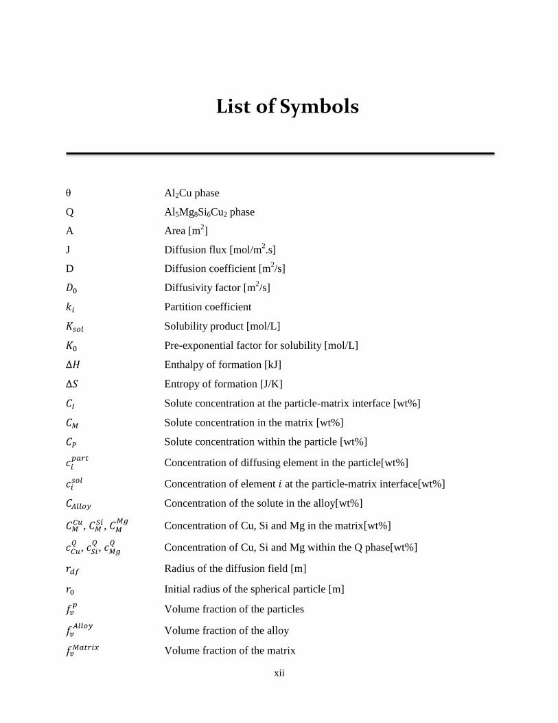
The T6 heat treatment is illustrated in Figure 2.6 for an Al-Si-Cu alloy as an example. The
evolution of the microstructure is shown; from (1) atoms in solid solution at the solution
12
treatment temperature, through (2) a supersaturated solid solution at room temperature after
quench, to (3) precipitates formed at the artificial aging temperature [2].
The precipitation sequence for an Al-Si-Cu alloy, such as 319, is based upon the
formation of Al2Cu-based precipitates. The Al2Cu precipitation sequence is generally described
as follows: [18,38]
𝛼𝑠𝑠 → 𝐺𝑃 𝑍𝑜𝑛𝑒𝑠 → 𝜃″ → 𝜃′ → 𝜃 (𝐴𝑙2𝐶𝑢)
In Al-Si-Cu-Mg at high Mg levels (more than 6% [5]) Q and β phases may also form. Cu
can increase the fraction of the β″ phase formed, but it can also form the Q″ phase, which has a
lower strength contribution compared to the β″ phase. The β″ phase is therefore preferred, rather
than the Q″ phase [5,8,39]
Figure 2.6: T6 heat treatment of Al-Si-Cu alloys [5].
The time and temperature of aging treatment determines the number density, size, and
size distribution of precipitates [2]. Fine and dense precipitates with a smaller inter-particle

13
spacing are formed at a lower aging temperature of 150 °C compared to coarse, less dense and
more widely dispersed at higher temperature, i.e., 250 °C. The strength of 319 alloys increases
with the Mg content and decreases with Sr and aging temperature and time [40]. It is been
reported that the precipitates that predominate at the peak aging of cast A319 aluminum alloy
(Al–4.93 wt%Si–3.47 wt%Cu) after solution treatment at 500 ± 5 °C for 8 h and aging at 170 ± 5
°C for 24 h are coherent θ″ together with semi-coherent θ′ at lower number density. It is been
suggested that θ″ is mainly responsible for peak aging in cast A319 aluminum alloy [41,42].
Dislocation density affects aging response. These dislocations form during quenching. θ′
phase forms on dislocation while θ″ forms somewhere in the bulk [43]. The more the dislocation
density, the higher the fraction of θ′; so the strength of the alloy is lower. The strength of an age-
hardenable alloy is governed by the interaction of moving dislocations and precipitates. The
obstacles in precipitation hardened alloys which hinder the motion of dislocations may be either
the strain field around the GP zones resulting from their coherency with the matrix, or the zones
and precipitates themselves, or both. The dislocations are then forced to cut through them or go
around them forming loops.
When the alloy is naturally aged prior to artificially aging, age hardening response would
be slower, but the time to peak and the peak hardness will remain unaffected.A pre-step aging at
lower temperature after solution treatment and then aging at the regular temperature, results in
improved mechanical properties because pre-aging causes finer dispersion of precipitates. This is
due to the fact that higher density of precipitates leads to the lower inter-precipitates spacing in
which dislocations bow. However, the single step still has remained the most economical temper
in terms of hardness [44].
2.3 Modelling dissolution during homogenization
Modelling can facilitate the design of an alloy and its heat treatment process, which
meets specified requirements for a certain component. Development of models can also help in
the search for new alloys as knowledge is gained about the influence of the microstructure on the
alloy properties.
Two processes are involved in the dissolution of a precipitate: 1) atom transfer across the
interface separating the matrix and the precipitate phase (interface diffusion) and 2) diffusion of
the solutes away from the interface (long range diffusion) [45]. There are two limiting cases; 1)

14
the dissolution rate is limited by long range solute diffusion through the matrix and 2) the
transfer of atoms across the matrix-precipitate interface controls the dissolution rate. In the
former case local interfacial equilibrium exists while in the latter it does not, and the rate of
dissolution is controlled by and interfacial reaction.
The time needed for the dissolution of secondary phases and homogenization of the as-
cast microstructure during a post casting heat treatment can be modelled using various
approaches. Dissolution of second phase particles was first modelled by Aaron [46]. He assumed
that the dissolving particle is in equilibrium with the matrix and as the particle dissolves the re-
equilibrium at the particle-matrix interface to the new equilibrium concentration occurs rapidly
in comparison to other processes involved in the dissolution.
𝑑𝑅(𝑡)
𝑑𝑡=
𝐾2𝐷
2[𝑅(𝑡) − 𝑅0] (2.1)
In the above equation 𝑅(𝑡) is the precipitate radius or half-thickness as a function of time (t)
during dissolution, K is a material constant, D is the volume interdiffusion coefficient andR0 is
the radius or half thickness of the initial particle. In the model developed by Aaron just the
steady state part is taken into account.
After Aaron, Whelan [47] considered both the steady state and transient parts of the
dissolution kinetics. He considered the precipitate-matrix interface to be stationary and found the
dissolution rate of a spherical particle as follows:
𝑑𝑅
𝑑𝑡= −
𝑘𝐷
2𝑅−𝑘
2√𝐷
𝜋𝑡 (2.2)
Where 𝑘 = 2(C𝐼 − C𝑀) (C𝑃 − C𝐼)⁄ , 𝑅 is the radius of the precipitate and 𝐷 is the diffusion
coefficient. The term in R-1
on the right of equation (2-2) arises from the steady state part of the
diffusion field. The term t-1/2
arises from the transient part.
In most alloy systems of interest, |𝑘| < 0.3, and it has been shown that for small values
of k, the stationary interface is a good assumption. It is noteworthy to say that for small values of
k it is concentration inequality 𝐶𝑃 − 𝐶𝑀 ≫ 𝐶𝐼 − 𝐶𝑀 rather than slow interface reaction that
guarantees R(t) to be slowly varying as a function of time [48]. A small value of k means that the

15
concentration of the alloying elements in the particle is so large compared to the solubility of
them in the matrix that atoms can diffuse away from the particle without causing a rapid
movement of the particle/matrix interface [49].
When the transient part is zero such as over long times for the range of 𝑟 < ~2000�̇� and
small rate constant (k), Thomas and Whelan have shown that the dissolution rate can be found
according to equation (2-3) [46,50].
𝑑(𝑟2)
𝑑𝑡= −𝑘𝐷 (2.3)
Nolfi et al. [51] broadened the model developed by Whelan. They considered the effect
of interfacial reactions as well and defined a parameter named σ which specifies the
thermodynamic state of the interface:
𝜎 = (𝐾𝑅0𝐷+ 1)
−1
(2.4)
Where 𝐾 is the reaction rate constant, 𝐷 is the diffusivity of solutes in matrix and 𝑅0 is the
precipitated radius. If 𝐾 is infinite then local equilibrium prevails; if 𝐾 deviates infinitesimally
from zero, then interfacial reactions are rate controlling. For intermediate values of 𝐾, mixed
mode occurs.
Aaron and Kotler in 1971 [48] introduced the effect of particle surface curvature
according to the well-known Gibbs-Thompson effect and figured out that the influence of
curvature is negligible unless the difference between the solute concentration at the particle-
matrix interface and the matrix concentration is sufficiently small. In this case, the presence of
curvature tends to speed up dissolution, being particularly important at long times (i.e. small
precipitate sizes).
Brown in 1976 [52] considered the effect of morphology on the dissolution kinetics. He
considered spherical, cylindrical and planar shapes. The dissolution time for cylindrical particle
lies in between of spherical and planar but closer to the spherical shape. He also showed that
there is a progressive decrease in the dissolution time with increasing saturation which is due to
the fact that the concentration gradient at the phase interface increases with increasing saturation
(Figure 2.7).

16
Figure 2.7: Dissolution times for planar, spherical and cylindrical precipitates as a function of saturation,
CA [52].
Tundal and Ryum in 1992 [49] introduced the idea of having a size distribution in
particles instead of having an array of particles with equal size. It was found that small particles
decrease in size at higher rate than large particles which makes the presence of a size distribution
in particles to greatly influence the dissolution kinetics.
Singh and Flemings [38] considered a plate-like dendrite morphology, having an initial
sinusoidal composition distribution in the primary phase and constant second phase composition.
According to their model the expression which relates volume fraction of the second phase to
solution time is:
𝑔 + 𝑎
𝑔0 + 𝑎= exp (−
𝐷𝑡
𝑙02 .𝜋2
4) (2.5)
Where 𝑔 and 𝑔0 are the volume fraction of the second phase at time t and t=0, respectively, D is
the diffusion coefficient at the solution temperature, 𝑙0 is one half secondary dendrite arm
spacing, t is the time of solution treatment, 𝑎 = 𝐶𝑀− 𝐶0
𝐶𝛽 , 𝐶𝑀 is the maximum solubility at
solution temperature, 𝐶0 is the initial composition and 𝐶𝛽 is composition of 𝛽 phase.
The critical time for complete solutionizing, 𝑡𝑐, is obtained by setting 𝑔 = 0
𝑡𝑐 = 4𝑙02
𝜋2𝐷ln𝑔0 + 𝑎
𝑎 (2.6)

17
Teleshov and Zolotorevsky [53] also derived an approximate expression for the time
required for total dissolution of the second phase. Composition of the second phase was assumed
constant and interface motion was neglected. This analysis is a solution to Fick’s first law using
a mean concentration gradient, ∆𝐶/∆𝑋, where the effective diffusion distance, ∆𝑋, is estimated
from the particle/matrix interface area, 𝑆, and the dendrite arm spacing, 𝑑. Assuming a plate-like
morphology (𝑆 = 1/𝑙0), the time to dissolve the precipitates may be written as:
𝑡𝑐 = 𝑔0[𝐶𝛽 − 𝐶𝑀]
[(𝐶𝑀 − 𝐶0) + 𝑔0
2 (𝐶𝛽 + 𝐶𝑀)]
(𝑙02
𝐷) (2.7)
Rometsch [54] modelled the dissolution of binary second phase particle during solution
heat treatment. He considered equally sized spherical diffusion field around equally sized
particle, considering there are no other particles other than dissolving particles and that the
particle-matrix interface is not moving as particles dissolve. Based on these microstructural
simplifications, he developed a numerical finite difference model whose output is dissolution and
homogenization time. This model solves Fick’s first law in radial coordinates. He validated the
model for aluminum A356 and A357. The results are shown in Table 2.1.
Table 2.1: Model predictions for A356 and A357 [54].
Alloy and condition Numerical model Experimental result
A356 Dissolution time 3 min 2-4 min
A356 Homogenization time 5.1 min 8-15 min
A357 Dissolution time 38.7 min <50 min
A357 Homogenization time 40.7 min <50 min
Vermolen [55-71] developed a model for multicomponent systems. He used the multi-
component version of Fick's second law (Equation 2.8) and for simplicity assumed that all
species diffuse independently, and that the diffusion coefficients are constant.

18
𝜕𝑐𝑖𝜕𝑡= 𝐷𝑖𝑟𝑎𝜕
𝜕(𝑟𝑎
𝜕𝑐𝑖𝜕𝑟) (2.8)
Here 𝐷𝑖and 𝑐𝑖, respectively, denote the diffusion coefficient and the concentration of the species
i, and a is a geometric parameter, which equals 0, 1, or 2 for a planar, a cylindrical, or a spherical
geometry, respectively. As all cross-diffusion coefficients are set to zero, this is a good
approximation for most (dilute) commercial alloys. The dissolution rate (interfacial velocity) is
obtained as follows:
𝑑𝑆(𝑡)
𝑑𝑡=
𝐷𝑖
𝑐𝑖𝑝𝑎𝑟𝑡 − 𝑐𝑖
𝑠𝑜𝑙
𝜕𝑐𝑖𝜕𝑆(𝑆, 𝑡) (2.9)
Where 𝑐𝑖𝑝𝑎𝑟𝑡
is the weight percent of diffusing element 𝑖 in the particle, 𝑐𝑖𝑠𝑜𝑙 is the concentration
of element 𝑖 at the particle-matrix interface and 𝑑𝑆 𝑑𝑡⁄ the velocity of boundary movement. He
found good agreement between the model and the analytical solution at shorter dissolution time,
while analytical results deviate from numerical results at longer times (Figure 2-8).
Figure 2.8: The interface position as a function of time during the dissolution of a planar phase obtained
for analytical and numerical solutions [60].

19
Sjölander [72] modelled the dissolution of Al2Cu phase in Al-Mg-Si-Cu alloys using
Fick’s second law. She found out that the dissolution process is diffusion-controlled [73].
Although there are various models for particle dissolution, most of them are applicable
for wrought alloys, and there has been less attention on cast alloys in literature. Cast alloys are
more complicated in terms of modelling as particle dissolution is accompanied by removal of
micro and macro segregation which adds difficulties in the model approximation.
Homogenization of cast AlB319 is complex due to concurrent dissolution of θ and Q phase. This
study captures the effect of segregation as well as secondary dendrite arm spacing on the particle
dissolution and further homogenization, and concurrent dissolution.

20
Chapter 3
3. Scope and objectives
The thermal processing of high-volume cast-aluminum engine blocks and cylinder head
components is a key concern of automotive engineers today. Heat treatment is an indispensable
step in manufacturing engine blocks, as mechanical properties are selectively controlled by
deliberate manipulation of the chemical and metallurgical structure of a component. However,
apart from the desired effects, the heat treatment process can be accompanied by unwanted
effects such as component distortion, high material’s hardness, low material’s strength and a lack
of toughness, which can lead to crack formation and fatigue failure. Therefore, success or failure
of heat treatment not only affects manufacturing costs but also determines product quality and
reliability. Hence, optimization of the heat treatment process is of great significance in the
industry due to the ever increasing energy costs and competition. Heat treatment must therefore
be taken into account during development and design, and it has to be controlled in the
manufacturing process. Part designers are looking for process feasibility, a specific
microstructure fitting to the in-service requirements, minimum part distortion, and proper
distribution of residual stresses. In simulation-based design and manufacturing it is desirable to
calculate the effects of heat treatment in advance and to optimize them by varying materials and
workpiece shape.
Cast Al-Si-Cu-Mg alloys are well studied in terms of the influence of different alloying
elements and modifiers on their microstructure and mechanical properties. Also, the solution heat
treatment and aging process that is done on these types of alloys is well investigated, and the
optimum solution heat treatment has been suggested. In addition, microstructural investigation
has been done on these alloys and the type of intermetallics and secondary phases that form are

21
well understood across the entire manufacturing process from casting through to age hardening
and final mechanical properties. However, modelling the homogenization process is the main
knowledge gap in this area that has remained relatively unstudied. There has been extensive
work done on modelling solution heat treatment of wrought aluminum alloys, while cast
aluminum alloys have less been studied. Althuogh Colley [74] devleoped a model for A356 to
examine the metallurgical changes during homogenization and subsequent aging, the alloy he
examined was by comparison much simpler as it only invovled the dissolution of Mg2Si. The
B319 alloy is much more complex and its homogenization involves the concurrent dissolution of
the Al2Cu and Q phases in addition to the Mg2Si.The benefit of developing models to predict
homogenization includes an improvement in our understanding of alloy behaviour during multi-
stage heat treatment, which in turn can enable process optimisation from the standpoint of the
material and result in lower variability in final component properties. This is particularly
important when casting large components with complex solidification patterns and non-uniform
as-cast microstructures that respond to solution treatment locally at different rates.
The aim of this work was to model the homogenization process of cast AlB319; this
includes dissolution of the secondary phases that are Al2Cu and Q, as well as the removal of
segregation. The effect of SDAS and homogenization temperature as well as the effect of two-
step heat treatment is investigated. The final model is then used so that a quantitative
understanding of the influence of the process parameters during casting and heat treatment of Al
B319 can be obtained.

22
Chapter 4
4. Modelling and Experimental Methods
In this study, the homogenization process applied to aluminum alloy B319 that consists
of the dissolution of secondary phases and the removal of segregation was modelled.
The metallurgical changes that occur during heat treatment of AlB319 were modelled
using MATLAB and COMSOL. MATLAB is a commercial software package that provides
users with an interactive development environment, so that you can use a high-level language as
well as built-in features to perform numerical computation, algorithm development, and
application development. COMSOL Multiphysics software, on the other hand, allows users to
customize and combine any number of physics, the way they want to.
To model the dissolution phenomena two approaches were applied; stationary interface
and moving boundary. In the former approach it is assumed that the particle-matrix interface is
stationary. In the latter it is assumed that by gradual dissolution of particle the boundary between
particle and matrix moves to accommodate for the particle diameter reduction.
Dissolution of the θ phase was modelled using MATLAB with a finite difference method
and COMSOL which uses a finite element method. Dissolution of the Q phase was modelled
using MATLAB. Also, the coupling effect of the θ and Q phases in dissolution time was
investigated using MATLAB.
Using the models, the effect of particle morphology (shape) and SDAS on the dissolution
time was examined. In the present study the geometries that are considered for the dissolving
particles are sphere, cylinder, plate and ellipse. Both two and three-dimensional models were
developed using COMSOL software. After the dissolution process was complete, the time

23
needed for complete removal of segregation was modelled to address the whole homogenization
process.
Finally, the models were validated through a series of experimental measurements using
conventional and fluidized sand bed furnaces for single-step and two-step heat treatment.
Qualitative analysis was done using Scanning electron microscope (SEM). Optical microscope
(OM) with image analysis software was utilized for quantitative analysis.
4.1 Model development
Particle dissolution is assumed to proceed by a number of subsequent steps:
decomposition of the chemical bonds in the particle, crossing of the interface by atoms from the
particle and long-distance diffusion in the matrix (Figure 4.1). It is assumed in the model that the
first two steps proceed sufficiently fast with respect to the long-distance diffusion that they do
not affect the dissolution kinetics.
Figure 4.1: A schematic presentation of the steps involved in the particle dissolution process.
4.1.1 Model assumptions
To simplify the model some assumptions should be made; these are as follows,
1) Particles are distributed evenly in the matrix, and have equal sizes and uniform
compositions.
2) Particles maintain their stoichiometric composition during the whole process of
dissolution.
Atom debonding
Atom transfer across
boundary
Diffusion through
the matrix
(1)
(2)
(3)

24
3) The rate of dissolution is limited by the long-range diffusion; hence, equilibrium is
always established at the interface between the particle and the matrix, and the
concentration of each element at the interface is equal to the solubility of that element at
the solutionizing temperature.
4) The diffusion coefficient, D, is independent of composition and the presence of the other
alloying elements. Hence, all cross-diffusion coefficients are set to zero. This is expected
to be a good assumption for dilute systems.
5) Soft impingement does not occur. Diffusion fields of particles do not interact. This
implies a dilute concentration of solute.
6) Diffusion only takes place inside the Al-rich phase. Precipitate phases are diffusion-free.
7) The model does not differentiate between blocky and eutectic Al2Cu phase.
8) The effect of convection has been neglected.
4.1.2 Description of the Models
Generally, for modelling the particle dissolution in a field based on diffusion, some
aspects are considered:
1- Selection of diffusion equation: 1- Fick’s First Law, 2- Fick’s Second Law.
2- Solution of equations: 1- finite difference, 2- finite element.
3- Solution of differential equations sets: 1- Explicit, 2- Implicit.
4- Meshing: 1- equal sizes, 2- different sizes by getting distance from the centre of the
diffusion field.
5- Movement of mesh: 1- Fixed Mesh 2- Moving Mesh.
6- Reduction of particle mass: 1- system mass conservation, 2- local mass conservation at
the interface and checking system mass conservation.
7- Number of components: 1- single component, 2- multi component.
8- Number of Phases: 1- single phase, 2- two or more phases.
9- Number of geometry dimension: 1- one, 2- two, 3- three.
10- Geometry coordination: 1-spherical, 2- cylindrical, 3- cartesian.
In this study three different approaches were selected such that all of these aspects are
considered.

25
1- Single Component Fixed Mesh (SCFM): In this method, Fick’s first Law for a single
component system is solved explicitly based on the finite difference method. In this
approach the mass of particle is reduced based on system mass conservation but the
radius of particle is remained fixed (Fixed Mesh). The time step is selected
automatically based on convergency criteria. This method is used only for spherical
one dimensional system.
2- Multi Component Moving Mesh (MCMM): In this method, Fick’s second Law for a
single or multi component system is solved implicitly based on finite difference
method. The mass of particle is reduced based on local mass conservation at the
interface, and the particle radius reduces based on moving mesh. This method is used
only for one dimensional spherical, cylindrical and planer systems but it can be used
for two phases that are coupled via fields variables.
3- COMSOL: COMSOL is a 3D finite element software which is used for multiphysics
modelling. In this study, two physic sections of the code were used: 1- Transport of
dilute species 2- Deformed geometry. The major advantage of this code is the
capability of simulation of complicated 3D geometries. However, this code cannot be
used for multicomponent systems directly. Therefore, the equation of the local mass
conservation at the interface must be solved separately with a User Defined Function
(UDF). Moreover, the system mass conservation is not conserved when local mass
conservation at the interface is used. Furthermore, moving mesh in complicated
geometries causes mesh distortion at the interface. Hence, two methods for particle
dissolution were proposed: 1- moving mesh based on system mass conservation for
simple geometries, and 2- fixed mesh for complicated geometries, while the average
concentration of the field is the major parameter for determination of the particle
mass.
4.1.3 Fixed mesh approach
A schematic of this approach for a spherical particle is shown in Figure 4.2. It can be
seen that the particle is dissolving the particle-matrix interface which is shown by red line is
being kept at its initial position.

26
Figure 4.2: A schematic presentation of stationary interface dissolution process for a spherical particle.
4.1.3.1 Governing equations
As-cast aluminum B319 has a dendritic microstructure. The intermetallic phases such as
iron or Cu precipitates (Al2Cu and Al5Mg8Cu2Si6) form at interdendritic spaces when cooling
from solidification temperature. Hence, one can relate interparticle spacing to secondary dendrite
arm spacing (SDAS). It is assumed that the particles are equally sized and surrounded by the
diffusion field in the matrix. In order to derive the relationship between SDAS and the size of
diffusion field, microstructure is divided into equally sized cubic cells as diffusion fields with the
particles at the centre. The size of these cubic cells is equal to SDAS.
In the case of spherical particles, we can use spherical diffusion field which its radius,
rdf, can be found by equalizing the volume of the cubic cell to the spherical equivalent one
(Figure 4.3),
Figure 4.3: A schematic of secondary phase particles location and the diffusion field around the particle.

27
rdf = √3SDAS3
4π
3
(4.1)
According to Romesch [54], if volume fraction of a particle is denoted by 𝑓𝑣𝑃 the particle radius,
𝑟𝑝, can be estimated as follow,
𝑟𝑝 = √3𝑓𝑣𝑃𝑆𝐷𝐴𝑆3
4𝜋
3
(4.2)
There are alloying elements such as Cu and Mg, and impurities such as iron (Fe) in the alloy.
Dissolution of the Al2Cu phase is controlled by the diffusion of Cu into the matrix, while
diffusion of Cu, Mg and Si are rate controlling in the dissolution of Al5Mg8Cu2Si6. The initial
average matrix concentration of each element, CM, can be determined from the alloy
concentration of that element, CA, and the volume fraction of the precipitate in the as-cast
microstructure as follows,
𝑀𝑎𝑡𝑟𝑖𝑥 𝑐𝑜𝑛𝑐𝑒𝑛𝑡𝑟𝑎𝑡𝑖𝑜𝑛 = 𝐴𝑙𝑙𝑜𝑦 𝑐𝑜𝑛𝑐𝑒𝑛𝑡𝑟𝑎𝑡𝑖𝑜𝑛 − 𝑃𝑎𝑟𝑡𝑖𝑐𝑙𝑒 𝑐𝑜𝑛𝑐𝑒𝑛𝑡𝑟𝑎𝑡𝑖𝑜𝑛
𝐶𝑀𝑎𝑡𝑟𝑖𝑥𝜌𝑀𝑎𝑡𝑟𝑖𝑥𝑓𝑣
𝑀𝑎𝑡𝑟𝑖𝑥 = 𝐶𝐴𝑙𝑙𝑜𝑦𝜌𝐴𝑙𝑙𝑜𝑦𝑓𝑣
𝐴𝑙𝑙𝑜𝑦− 𝐶𝜃𝜌
𝜃𝑓𝑣𝜃 (4.3)
For Al2Cu:
Since 𝑓𝑣𝐴𝑙𝑙𝑜𝑦
= 1 and 𝐶𝜃 = 𝑤𝑡%𝐶𝑢𝜃,
𝐶𝑀𝐶𝑢 = [𝐶𝐴
𝐶𝑢 − (𝑓𝑣𝜃 ∗
𝜌𝜃
𝜌𝐴𝑙𝑙𝑜𝑦∗ 𝑤𝑡%𝐶𝑢𝜃 − 𝑓𝑣
𝑄 ∗ 𝜌𝑄
𝜌𝐴𝑙𝑙𝑜𝑦∗ 𝑤𝑡%𝐶𝑢𝑄)] ∗
1
𝑓𝑣𝑀𝑎𝑡𝑟𝑖𝑥
(4.4)
Where 𝜌𝜃, 𝜌𝑄 and 𝜌𝐴𝑙𝑙𝑜𝑦 are the Al2Cu, Q and alloy densities, respectively. 𝑤𝑡%𝐶𝑢𝜃is the
weight percent of Cu in a stoichiometric Al2Cu particle. 𝑓𝑣𝑀𝑎𝑡𝑟𝑖𝑥is the volume fraction of matrix
which is assumed to be 1 − 𝑓𝑣𝜃− 𝑓𝑣
𝐹𝑒 𝑖𝑛𝑡.𝑚𝑡𝑙.− 𝑓𝑣𝑆𝑖 𝑒𝑢𝑡.. Where 𝑓𝑣
𝐹𝑒−𝑖𝑛𝑡.𝑚𝑡𝑙 and 𝑓𝑣𝑆𝑖−𝑒𝑢𝑡. are the
volume fraction of Fe intermatallics and Si eutectic, respectively. It is assumed that there are just
Al2Cu precipitates present in the alloy.
For the Q phase,

28
𝐶𝑀𝐶𝑢 = [𝐶𝐴
𝐶𝑢 − (𝑓𝑣𝑄 ∗
𝜌𝑄
𝜌𝐴𝑙𝑙𝑜𝑦∗ 𝑤𝑡%𝐶𝑢𝑄 − 𝑓𝑣
𝜃 ∗ 𝜌𝜃
𝜌𝐴𝑙𝑙𝑜𝑦∗ 𝑤𝑡%𝐶𝑢𝜃)] ∗
1
𝑓𝑣𝑀𝑎𝑡𝑟𝑖𝑥
(4.5)
𝐶𝑀𝑆𝑖 = [𝐶𝐴
𝑆𝑖 − (𝑓𝑣𝑄 ∗
𝜌𝑄
𝜌𝐴𝑙𝑙𝑜𝑦∗ 𝑤𝑡%𝑆𝑖𝑄 − 𝑓𝑣
𝐹𝑒 𝑖𝑛𝑡.𝑚𝑡𝑙. ∗ 𝜌𝐹𝑒 𝑖𝑛𝑡.𝑚𝑡𝑙.
𝜌𝐴𝑙𝑙𝑜𝑦∗ 𝑤𝑡%𝑆𝑖𝑖𝑛𝑡.𝑚𝑡𝑙.
− 𝑓𝑣𝑆𝑖 𝑒𝑢𝑡𝑒𝑐𝑡𝑖𝑐 ∗
𝜌𝑆𝑖 𝑒𝑢𝑡𝑒𝑐𝑡𝑖𝑐
𝜌𝐴𝑙𝑙𝑜𝑦∗ 𝑤𝑡%𝑆𝑖𝑆𝑖 𝑒𝑢𝑡𝑒𝑐𝑡𝑖𝑐)] ∗
1
𝑓𝑣𝑀𝑎𝑡𝑟𝑖𝑥
(4.6)
𝐶𝑀𝑀𝑔= [𝐶𝐴
𝐶𝑢 − (𝑓𝑣𝑄 ∗
𝜌𝑄
𝜌𝐴𝑙𝑙𝑜𝑦∗ 𝑤𝑡%𝑀𝑔𝑄)] ∗
1
𝑓𝑣𝑀𝑎𝑡𝑟𝑖𝑥
(4.7)
Where 𝑤𝑡%𝐶𝑢𝑄, 𝑤𝑡%𝑆𝑖𝑄 and 𝑤𝑡%𝑀𝑔𝑄 are the weight percent of Cu, Si and Mg in a
stoichiometric Al5Mg8Cu2Si6 particle.
The diffusion field is divided into shells which surround the particle and are increasing in
size by dr (Figure 4.4).
Figure 4.4: The diffusion field around particle and the diffusion shells.
Mass transport across the boundaries is given by:
𝑚
𝜌= 𝑗. 𝐴. 𝑡 (4.8)
And according to Fick`s first law
Particle
Shell (dr)
Diffusion field

29
𝑗 = −𝐷𝜕𝑐
𝜕𝑟 (4.9)
𝐷is defined according to the well-known Arrhenius relationship
𝐷 = 𝐷0 exp (−𝑄
𝑅𝑇) (4.10)
Where 𝑄 is the activation energy for diffusion of element in the matrix.
So one can calculate the mass transfers in and out of each shell,
𝑚 = 𝐷𝜌 𝜕𝑐
𝑑𝑟4𝜋𝑟2𝑡 (4.11)
𝑚𝑖𝑛 = 𝐷 [(𝐶𝑛−1 − 𝐶𝑛)𝜌
𝐴𝑙𝑙𝑜𝑦
𝑑𝑟] 4𝜋(𝑟𝑛−1)
2𝑑𝑡 (4.12)
𝑚𝑜𝑢𝑡 = 𝐷 [(𝐶𝑛 − 𝐶𝑛+1)𝜌
𝐴𝑙𝑙𝑜𝑦
𝑑𝑟] 4𝜋(𝑟𝑛)
2𝑑𝑡 (4.13)
4.1.3.2 Initial conditions
The initial concentration of each element in matrix is set to 𝑐𝑖𝑀 and the concentration of
the element at the particle-matrix interface is 𝑐𝑖𝑠𝑜𝑙.
𝑐𝑖(𝑟, 0) = 𝑐𝑖𝑀 𝑟𝑝 < 𝑟 ≤ 𝑟𝑑𝑓 (4.14)
𝑐𝑖(𝑟, 0) = 𝑐𝑖𝑠𝑜𝑙 𝑟 = 𝑟𝑝 (4.15)
The model requires that 𝑐𝑖𝑠𝑜𝑙 be greater than 𝑐𝑖
𝑀 otherwise instead of dissolution growth
will occur. This situation is demonstrated in Figure 4.5. As the particle dissolves the
concentration profile in the diffusion field around the particle is changing according to Figure
4.6, where Cu concentration in particle, interface and alloy is shown by CP, Csol
and CA,
respectively.

30
Figure 4.5: A schematic presentation of the situation in which particle growth occurs instead of
dissolution.
Figure 4.6: A schematic presentation of the Concentration profile in the matrix around particle as
dissolution time elapses.
4.1.3.3 Boundary conditions
Since it is assumed that we have equally sized diffusion fields that stay unchanged in
size, and there is not any impingement of diffusion filed into each other, so there is no flux at the
outer boundary of the diffusion field.
𝜕𝑐𝑖𝜕𝑟= 0 𝑟 = 𝑟𝑑𝑓 (4.16)
𝑐𝑖𝑠𝑜𝑙
𝑐𝑖𝑀
Cu concentration
Csol
CP
CA
Distance
CA
CP
Distance
Cu concentration
CP
CA
Distance
Cu concentration
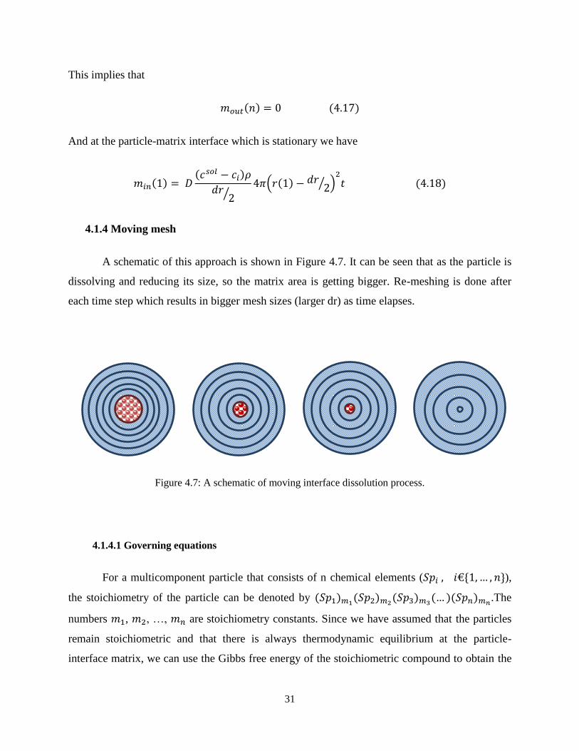
31
This implies that
𝑚𝑜𝑢𝑡(𝑛) = 0 (4.17)
And at the particle-matrix interface which is stationary we have
𝑚𝑖𝑛(1) = 𝐷(𝑐𝑠𝑜𝑙 − 𝑐𝑖)𝜌
𝑑𝑟2⁄
4𝜋(𝑟(1) − 𝑑𝑟 2⁄ )2
𝑡 (4.18)
4.1.4 Moving mesh
A schematic of this approach is shown in Figure 4.7. It can be seen that as the particle is
dissolving and reducing its size, so the matrix area is getting bigger. Re-meshing is done after
each time step which results in bigger mesh sizes (larger dr) as time elapses.
Figure 4.7: A schematic of moving interface dissolution process.
4.1.4.1 Governing equations
For a multicomponent particle that consists of n chemical elements (𝑆𝑝𝑖 , 𝑖€{1,… , 𝑛}),
the stoichiometry of the particle can be denoted by (𝑆𝑝1)𝑚1(𝑆𝑝2)𝑚2(𝑆𝑝3)𝑚3(… )(𝑆𝑝𝑛)𝑚𝑛.The
numbers 𝑚1, 𝑚2, …, 𝑚𝑛 are stoichiometry constants. Since we have assumed that the particles
remain stoichiometric and that there is always thermodynamic equilibrium at the particle-
interface matrix, we can use the Gibbs free energy of the stoichiometric compound to obtain the

32
hyperbolic relationship for the interfacial concentrations. The interfacial concentration of species
𝑖 is denoted by 𝑐𝑖𝑠𝑜𝑙.
(𝑐1𝑠𝑜𝑙)
𝑚1(𝑐2𝑠𝑜𝑙)
𝑚2(… )(𝑐𝑛𝑠𝑜𝑙)𝑚𝑛 = 𝐾𝑠𝑜𝑙 = 𝐾𝑠𝑜𝑙(𝑇) (4.19)
The factor K is referred to as solubility product. It depends on temperature 𝑇 according to an
Arrhenius relationship
𝐾 = 𝐾0 exp (−∆𝐻
𝑅𝑇) (4.20)
We denote the position of the moving particle-matrix interface by R(t) which extends from 0 to
𝑟𝑑𝑓.
Transportation of each solute element in a finite matrix, 𝑀(𝑡) = (𝑅(𝑡), 𝑟𝑑𝑓) with R(t)
the moving boundary and 𝑟𝑑𝑓 the fixed boundary, is described as follow,
𝜕𝑐𝑖(𝑟, 𝑡)
𝜕𝑡=𝐷𝑖𝑟𝑎𝜕
𝜕𝑟{𝑟𝑎
𝜕𝑐𝑖(𝑟, 𝑡)
𝜕𝑟} (4.21)
Where Di and ci are the diffusion coefficient and the concentration of the species 𝑖 in the matrix.
ci(r, t) is continuous, and has continuous derivatives with respect to t and r. The geometry is
planar, cylindrical and spherical for respectively a = 0; 1 and 2. The particle-matrix interface,
R(t), moves due to the mass balance which yields:
∫ 𝑐𝑖(𝑟, 𝑡)𝑟𝑎𝑑𝑟 = 𝑐𝑖
𝑝 . 𝑅𝑎+1
𝑎 + 1+ ∫ 𝑐𝑖(𝑟, 𝑡)𝑟
𝑎𝑑𝑟𝑟𝑑𝑓
𝑟=𝑅(𝑡)
𝑟𝑑𝑓
𝑟=0
(4.22)
Differentiating with respect to t of Equation 4.22 and using Equation 4.21, Equation 4.23 can be
obtained which is used to find the dissolution rate or the position of the moving boundary.
𝑑
𝑑𝑡{∫ 𝑐𝑖(𝑟, 𝑡)𝑟
𝑎𝑑𝑟 = 𝑐𝑝 . 𝑅𝑎+1
𝑎 + 1+ ∫ 𝑐𝑖(𝑟, 𝑡)𝑟
𝑎𝑑𝑟𝑟𝑑𝑓
𝑟=𝑅(𝑡)
𝑟𝑑𝑓
𝑟=0
}
0 = 𝑐𝑖𝑝 𝑎 + 1
𝑎 + 1𝑅𝑎𝑑𝑅
𝑑𝑡+ ∫
𝑑𝑐𝑖(𝑟, 𝑡)
𝑑𝑡𝑟𝑎𝑑𝑟
𝑟𝑑𝑓
𝑟=𝑅(𝑡)
+ ∫ 𝑐𝑖(𝑟, 𝑡)𝑑𝑟𝑎
𝑑𝑡𝑑𝑟
𝑟𝑑𝑓
𝑟=𝑅(𝑡)

33
0 = 𝑐𝑖𝑝𝑅𝑎
𝑑𝑅
𝑑𝑡+ ∫
𝐷𝑖𝑟𝑎𝜕
𝜕𝑟{𝑟𝑎
𝜕𝑐𝑖(𝑟, 𝑡)
𝜕𝑟} 𝑟𝑎𝑑𝑟 + ∫ 𝑐𝑖(𝑟, 𝑡)
𝑑𝑟𝑎
𝑑𝑟
𝑑𝑟
𝑑𝑡𝑑𝑟
𝑟𝑑𝑓
𝑟=𝑅(𝑡)
𝑟𝑑𝑓
𝑟=𝑅(𝑡)
0 = 𝑐𝑖𝑝𝑅𝑎
𝑑𝑅
𝑑𝑡+ 𝐷𝑖𝑟
𝑎𝜕𝑐𝑖(𝑟, 𝑡)
𝜕𝑟 + 𝑐𝑖(𝑟, 𝑡)𝑟
𝑎𝑑𝑟
𝑑𝑡
0 = 𝑐𝑖𝑝𝑅𝑎
𝑑𝑅(𝑡)
𝑑𝑡− 𝐷𝑖𝑅
𝑎𝜕𝑐𝑖(𝑟, 𝑡)
𝜕𝑟− 𝑐𝑖
𝑠𝑜𝑙𝑅𝑎𝑑𝑅(𝑡)
𝑑𝑡
𝑑𝑅(𝑡)
𝑑𝑡=
𝐷𝑖
𝑐𝑖𝑝 − 𝑐𝑖
𝑠𝑜𝑙
𝜕𝑐𝑖𝜕𝑟(𝑟, 𝑡) (4.23)
4.1.4.2 Boundary conditions
Fixed boundary
As it is assumed that we have equally sized diffusion fields that stay unchanged in size
and there is not any soft-impingement of diffusion filed into each other, so there is no flux at the
outer boundary of the diffusion field. For cases of low overall concentrations in the alloy, the cell
size 𝑟𝑑𝑓 may be large, and solution resembles the case where 𝑟𝑑𝑓 is infinite.
𝜕𝑐
𝜕𝑟= 0 𝑟 = 𝑟𝑑𝑓 (4.24)
Moving boundary
At the moving interface 𝑅(𝑡) we have the ‘‘Dirichlet boundary condition’’ for each
alloying element. The concentration of element 𝑖 in the particle is denoted by 𝑐𝑖𝑠𝑜𝑙; this
concentration is fixed at all stages. This assumption follows from the constraint that the
stoichiometry of the particle is maintained during dissolution. As dissolution continues, particle
size reduces. It is assumed that the dissolution process is diffusion-controlled, hence it is
assumed that the material is always at its thermodynamic equilibrium at the precipitate-matrix
phase interface. Therefore, the boundary condition is:
𝑐𝑖(𝑅(𝑡), 𝑡) = 𝑐𝑖𝑠𝑜𝑙(𝑟, 𝑡) 0 < 𝑡 < ∞ (4.25)
Therefore for Q phase it can be obtained that,

34
𝑐𝐶𝑢(𝑟, 𝑡) = 𝑐𝐶𝑢𝑠𝑜𝑙
𝑐𝑆𝑖(𝑟, 𝑡) = 𝑐𝑆𝑖𝑠𝑜𝑙
𝑐𝑀𝑔(𝑟, 𝑡) = 𝑐𝑀𝑔𝑠𝑜𝑙
𝐷𝐶𝑢
𝑐𝐶𝑢𝑄 − 𝑐𝑆𝑖
𝑠𝑜𝑙
𝜕𝑐𝐶𝑢𝜕𝑟
(𝑟, 𝑡) = 𝐷𝑆𝑖
𝑐𝑆𝑖𝑄 − 𝑐𝑆𝑖
𝑠𝑜𝑙
𝜕𝑐𝑆𝑖𝜕𝑟
(𝑟, 𝑡) =𝐷𝑀𝑔
𝑐𝑀𝑔𝑄 − 𝑐𝑀𝑔
𝑠𝑜𝑙
𝜕𝑐𝑀𝑔
𝜕𝑟(𝑟, 𝑡) (4.26)
Equation 4.26 follows local mass-conservation of the components. The unknowns in above
equations are the concentrations 𝑐𝑖, interfacial concentrations 𝑐𝑖𝑠𝑜𝑙 and the interfacial position
𝑅(𝑡).
4.1.4.3 Model consistency assessment
It is required that the total mass of all elements is constant in the whole dissolution cell,
i.e. over 0 ≤ 𝑟 ≤ 𝑟𝑑𝑓. If let 𝑐𝑖𝑀 be constant in matrix, then
∫ 𝑐𝑖(𝑟, 𝑡)𝑟𝑎𝑑𝑟
𝑟𝑑𝑓
0
= 𝑐𝑖𝑝 𝑆0
𝑎+1
𝑎 + 1+ 𝑐𝑖
𝑀𝑟𝑑𝑓
𝑎+1 − 𝑆0𝑎+1
𝑎 + 1 (4.27)
Subtraction of ∫ 𝑐𝑖𝑀𝑟𝑎𝑑𝑟 = 𝑐𝑖
0𝑟𝑑𝑓0
𝑟𝑑𝑓𝑎+1
𝑎+1 from both sides of above equation gives
∫ (𝑐𝑖(𝑟, 𝑡) − 𝑐𝑖0)
𝑟𝑑𝑓
0
𝑟𝑎𝑑𝑟 = (𝑐𝑖𝑝 − 𝑐𝑖
𝑀) (4.28)
4.1.5 COMSOL
First of all the geometry of the particles needs to be defined. Four different geometries
were considered; spherical, planar, cylindrical and elliptical geometries. The diffusion equation
(Equation 4.24) is solved using finite difference method to find the concentration profile after
each time step. The mesh structure that is used is shown in Figure 4.8. The mesh quantification is
shown in Table 4.1. For two-dimensional models finer and fine meshes and for three dimensional
modelling normal and coarse meshes were used.

35
𝜕𝑐𝑖𝜕𝑡+ ∇. (−𝐷𝑖∆𝑐𝑖) = 0 (4.29)
Figure 4.8: Mesh used in COMSOL.
Table 4.1: COMSOL mesh quantification.
Mesh Number of elements
Number of elements
Area of the diffusion field [𝑚𝑚−2]
Extremely fine 24488 6.87E+03
Extra fine 6540 1.83E+03
finer 2072 5.81E+02
fine 1272 3.57E+02
normal 910 2.55E+02
coarse 436 1.22E+02
coarser 286 8.02E+01
Ultra coarse 128 3.59E+01
Extremely coarse 100 2.81E+01
Finer Fine
Normal Coarse

36
4.2 Morphology analysis
4.2.1 COMSOL
COMSOL software is used for analysis of the effect of morphology on the particle
dissolution. In this method, the radius of the field, 𝑟𝑠, is calculated based on constant volume (3-
D modelling) or constant area (2-D modelling). Therefore, we have
𝑆𝐷𝐴𝑆3 = 4/3𝜋𝑟𝑠𝑠3 = 𝑎3 = 𝜋𝑟𝑠𝑐
2ℎ = 4/3𝜋𝑎𝑏𝑐 (4.30)
𝑆𝐷𝐴𝑆2 = 𝜋𝑟𝑠2 = 𝑎2 = 𝜋𝑎𝑏 (4.31)
In the model it was assumed that ℎ = 2𝑟𝑠 for cylindrical geometry.
4.2.2 MATLAB
To investigate the effect of morphology on the particle dissolution, MCMM method is
applied for spherical, cylindrical and planar shapes. It should be noted that MCMM solves the
diffusion equation in 1-D. Therefore the height of the particle and field (for cylinder or planar) is
assumed to be equal.
For calculation of 𝑟𝑠 (radius of the diffusion field) in spherical coordination, following equation
is used
𝑆𝐷𝐴𝑆3 = 𝑉𝑠 =4
3𝜋𝑟𝑠
3, 𝑟0 = 𝑟𝑠(𝐹𝑣𝑏)1/3 (4.32)
For calculation of 𝑟𝑠 (radius of field circle) in cylindrical coordination, we can use two
approaches.
1) Constant volume with assigning cylinder height as a function of radius
𝐻𝑠 = 𝐻0 = 𝑟𝑠 → 𝑆𝐷𝐴𝑆3 = 𝑉𝑐 = 𝜋𝑟𝑠
3, 𝑟0 = 𝑟𝑠(𝐹𝑣𝑏)1/2 (4.33)
2) Constant area
𝑆𝐷𝐴𝑆2 = 𝐴𝑐 = 𝜋𝑟𝑠2, 𝑟0 = 𝑟𝑠(𝐹𝑣𝑏)
1/2 (4.34)
For calculation of 𝑟𝑠 in planar coordination, we can use three approaches.

37
1) Constant volume in which height and width are functions of radius
𝐻𝑠 = 𝐻0 = 𝑊0 = 𝑊𝑠 = 2𝑟𝑠 → 𝑆𝐷𝐴𝑆3 = 𝑉𝑝 = 8𝑟𝑠
3, 𝑟0 = 𝑟𝑠𝐹𝑣𝑏 (4.35)
2) Constant area in which the width is a function of radius
𝑊0 = 𝑊𝑠 = 2𝑟𝑠 → 𝑆𝐷𝐴𝑆2 = 𝐴𝑝 = 4𝑟𝑠
2, 𝑟0 = 𝑟𝑠𝐹𝑣𝑏 (4.36)
3) Constant interface
𝑆𝐷𝐴𝑆 = 𝐼𝑝 = 2𝑟𝑠, 𝑟0 = 𝑟𝑠𝐹𝑣𝑏 (4.37)
4.3 Thermodynamic analysis
First of all we need to analyze the alloy thermodynamically. A thermodynamic analysis
was conducted using FactSage and ThermoCalc software to obtain phase diagram and predict the
stability of different phases. These are our guidance tools to establish the temperature ranges
over which the phase dissolution occurs and equilibrium concentrations at the particle-matrix
interface in the matrix. Figure 4.9 to 4.11 illustrate the results of this analysis. It is seen in Figure
4.9 that the temperature range for dissolution is 475 °C - 505 °C. As shown in Figure 4.10, the
equilibrium phases and the temperature ranges in which they are present are Al2Cu, up to 465°C;
Al5Cu2Mg8Si6 (i.e., Q phase), up to 534°C and Iron phase, up to 616 °C. This implies that at
solution temperatures of 480 °C and 500 °C for the holding temperature of long enough Al2Cu
will completely dissolve but Q phase will be present to some extent after solution treatment as
well as iron phase. It should also be noted that solution treatment temperature cannot be over 505
°C as Cu rich phases start to melt. Also, from the phase diagram we can obtain that at 480 °C and
500 °C the Cu concentration at the interface in the matrix is 3.1 and 3.7, respectively.
After finding an appropriate dissolution temperature, we need to find the diffusivity of
the elements present in each phase. For the dissolution of Al2Cu phase there is just Cu that
diffuses, however, for the dissolution of Al5Mg8Si6Cu2, Cu, Mg and Si are the elements which
control the dissolution rate. The diffusivity of these elements in Al [75] is shown in Figure 4.11.
Although a clear trend of diffusivity: 𝐷𝑆𝑖 > 𝐷𝑀𝑔 > 𝐷𝐶𝑢 is seen in this figure, however, at the
dissolution temperatures of 480 °C to 500 °C, which correspond to 1000/T of 1.29 to 1.32, the

38
diffusivity of these elements in Al are so close to each other that we can say all of them are rate
controlling in the dissolution of Q phase.
Figure 4.9: Phase diagram of AlB319.
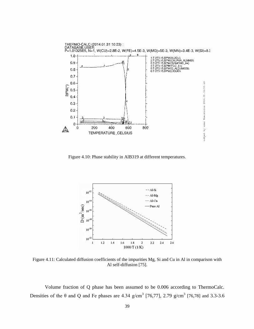
39
Figure 4.10: Phase stability in AlB319 at different temperatures.
Figure 4.11: Calculated diffusion coefficients of the impurities Mg, Si and Cu in Al in comparison with
Al self-diffusion [75].
Volume fraction of Q phase has been assumed to be 0.006 according to ThermoCalc.
Densities of the θ and Q and Fe phases are 4.34 g/cm3 [76,77], 2.79 g/cm
3 [76,78] and 3.3-3.6

40
g/cm3 [76,77], respectively. Seifeddine et al. [79] found the density of Al-Si alloys with different
concentrations of Cu added. The results are shown in Fig. 4.12.a. according to them the density
of the B319 alloy that is used in this study is 2.73 g/cm3. Nikanorov et al. [80,81] measured the
density of Al-Si alloys for different Si content and their results is shown in Figure 4.12.b.
According to EDS results there is 65% Si in the Si eutectic phase. By extrapolating the graph in
Figure 4.12.b, we can obtain the density of Si eutectic phase which is 2.42 g/cm3.
The enthalpies and entropies of formation of θ and Q phases and accordingly their
solubility products, which can be calculated according to Equation 4.30, are shown in Table 4.2.
𝐾 = 𝑒𝑥𝑝 (∆𝑆
𝑅−∆𝐻
𝑅𝑇) (4.38)
Figure 4.12: Density of Al-Si alloys at different a) Cu and b) Si content [80].
Table 4.2: Enthalpies, entropies and solubility products of the θ and Q phases.
∆𝐻 (𝐽
𝑚𝑜𝑙) ∆𝑆 (
𝐽
𝑚𝑜𝑙. 𝐾)
θ -19600 [82] -15.1 [83]
Q -12900 [84-86]
-16100 [86] -20 [86]
(a) (b)

41
4.4 Segregation analysis
As the alloy is a cast alloy there is microsegregation of solutes within the alloy which
means that the solute concentration in the central part of a dendrite arm changes gradually during
the solidification process, and we need to consider the effect of segregation in our model.
Therefore, the next step is to find the segregation ratio in a dendrite arm which is used in
calculating the initial concentrations of solute elements for the model. Sheil equation can be used
to find the segregation ratio in a dendrite arm [87].
𝑥𝑆 = 𝑘𝑥0𝐿(1 − 𝑓)−(1−𝑘) (4.39)
Scheil’s equation indicates that the concentration approaches infinity at the end of the
solidification process (𝑓 ≈ 1). The concentration gradient becomes very high and the driving
force for backdiffusion will increase. In this case the back diffusion in the solid phase cannot be
neglected. When back diffusion is taken into consideration it is necessary to modify Scheil’s
equation. Scheil’s modified equation for dendritic growth can be written as
𝑥𝑆 = 𝑘𝑥0𝐿 (1 −
𝑓
1 + 𝐷𝑠4𝜃
𝜆𝑑𝑒𝑛2
)
−(1−𝑘)
(4.40)
The quantity that has been used to describe segregation behaviour of an alloying element
is the segregation ratio which is the ratio of the highest and lowest values of the concentration of
the alloying element in a dendritic microstructure.
𝑆 = 𝑥𝑚𝑎𝑥𝑠
𝑥𝑚𝑖𝑛𝑠 (4.41)
S is the ratio of the highest and lowest values of the concentration of the alloying element in a
dendrite crystal aggregate. The expression for S has been calculated as in equation 4.24 which
shows microsegregation ratio,

42
𝑆 = 1
1 −
(
1 −
𝑘(1−2
𝜋𝑒−𝜋2𝐷𝑠𝜆𝑑𝑒𝑛2 𝑡𝑠𝑜𝑙
)
1−2𝑘
𝜋𝑒−𝜋2𝐷𝑠𝜆𝑑𝑒𝑛2 𝑡𝑠𝑜𝑙
)
𝑒−𝜋2𝐷𝑠
𝜆𝑑𝑒𝑛2 𝑡𝑠𝑜𝑙
(4.42)
In which 𝑡𝑠𝑜𝑙 is the solidification time, 𝜆𝑑𝑒𝑛 the primary dendrite arm spacing, 𝑘 the partition
coefficient, and 𝐷𝑠 the diffusion coefficient. The solidification time and primary dendrite spacing
are related to the cooling rate and can be defined as follow:
𝑡 = ∆𝑇
−𝑑𝑇 𝑑𝑡⁄ (4.43)
𝜆𝑑𝑒𝑛 = 𝐴 (−𝑑𝑇
𝑑𝑡)𝑛 (4.44)
The cooling rate can be found according to equation 4.27[88]:
log (𝑑𝑇
𝑑𝑡) = − [
log(𝑆𝐷𝐴𝑆) − 2.37
0.4] (4.45)
The partition coefficient for element 𝑖 can be found as follows,
𝑘𝑖 =𝐶𝑖𝑠
𝐶𝑖𝐿 (4.46)
Where 𝐶𝑖𝑠 and 𝐶𝑖
𝐿 are the concentration of the alloying element is solid and liquid, respectively.
The concentration of the alloying element is a function of both time and position. It can be found
by solving Fick’s second law for the diffusion process. If the origin (𝑦 = 0) is located at the
centre of a dendrite arm, the concentration of the alloying element in the solid phase can be
written as
𝑥(𝑦, 𝑡) = 𝑥𝑠/𝐿 − (𝑥𝑠/𝐿 − 𝑥𝑚𝑖𝑛)𝑒−4𝜋2𝐷𝑠𝜆2
𝑡𝑐𝑜𝑠
2𝜋𝑦
𝜆 (4.47)

43
Where 𝑥(𝑦, 𝑡), 𝑥𝑠/𝐿 and 𝑥𝑚𝑖𝑛 are the concentration of the alloying element (mole fraction), the
concentration of the alloying element in the solid at the interface at time t and 𝑥𝑚𝑖𝑛 the
concentration of the alloying element at the centre of the dendrite at time t, respectively. y is the
distance from the centre of the dendrite, which corresponds to the minimum concentration of the
solute, and λ is half of the SDAS and 𝐷𝑠 is the diffusion constant of the alloying element in solid.
4.5 Experiments
4.5.1 Wedge casing
The experimental work was done on a 319-type alloy, supplied in the form of industrially
cast ingots by Nemak Engineering Centre, Windsor, Ontario. These were remelted and cast into
a wedge mould at CANMET Materials Technology Laboratory located in Hamilton, Ontario. No
strontium or grain refiner additions were made to this alloy. A schematic of the wedge casting
geometry used at CANMET Materials is shown in Figure 4.13. Different distances from the end-
chill and correspondence microstructures are seen in the figure.
4.5.2 Chemical composition
The overall alloy composition, measured by an optical emission spectroscopy technique
is shown in Table 4.3. Metallographic specimens for investigation of the as-cast microstructure
were taken vertically from the bottom of the chill at distances of 12mm, 25mm, 50mm and
75mm.
Table 4.3: 319 chemical composition.
Element Al Si Cu Mg Fe Mn
Amount (wt%) Bal. 8.3 2.8 0.5 0.45 0.34

44
Figure 4.13: Schematic of the cast ingot showing the different sections’ microstructure (distances are in
mm).
4.5.3 Heat Treatment
Specimens for the heat treatment investigation were taken from a section of the casting
located at 25 mm and 60 mm vertically from the end chill. Specimen dimensions were
approximately 15mm (l) × 15mm (w) × 10mm (h). Solution heat treatments were done using
conventional furnace (CF) and fluidized sand bath (FB) at soak temperatures of 490 °C to 510 °C
12
50
25
75
100
225 µm
225 µm
225 µm
225 µm
225 µm

45
for various times up to 6 hours in CF and 2 hours in FB to investigate the effect of solution heat
treatment on dissolution of particles. Measurements when calibrating the CF showed that it takes
approximately 15 minutes for the samples to reach the set temperature. Therefore, samples are
exposed to an unavoidable non-isothermal heating process upon reaching to the desired
temperature, but considering the length of the overall homogenization process this represents a
minimal amount of time and can be ignored. Samples were then removed from the furnace and
immediately quenched into water at temperature of 21 °C.
4.5.4 Metallography and Image Analysis
All metallographic examinations were carried out on vertical sections perpendicular to
the solidification direction. The specimens were ground and polished using MD-Nap polishing
cloth with diamond suspension and MD-Chem cloths with colloidal silica suspensions to finish.
Microstructural investigations were done using optical and scanning electron microscopes.
Image quantification of area fraction for various phases was done on 2D images using image
analysis software. Secondary dendrite arm spacings in the as-cast material and volume fraction
of different particles present in the as-cast and heat treated specimens after different times were
measured using standard ASTM method. To measure the volume fraction 50 fields in a straight
line were examined.
As-cast and heat treated specimens were examined using SEM in secondary electron (SE)
mode with an accelerating voltage of 20 keV and working distance of 17 mm. EDS was done to
identify the various phases in the alloy.

46
Chapter 5
5. Results and Discussion
5.1 Microstructural investigations
The coarseness of the microstructure is characterized by SDAS which is determined by
the cooling rate from solidifying temperature. The average measured primary dendrite arm
spacing (PDAS), SDAS, particle sizes, interparticle spacing and volume fraction of different
phases at sections distanced 25, 60 mm and 115 mm from the end chill are shown in Table 5.1.
Table 5.1: As-cast microstructure parameters.
Distance
from end
chill (mm)
PDAS
(µm)
SDAS
(µm)
Al2Cu
size
(µm2)
Distance
between
particles
(µm)
Volume
fraction
of θ (%)
Volume
fraction
of Si
eutectic
Volume
fraction
of iron
phase
Si
eutectic
size (µm)
25 87 14 43.7 19.5 1.8 6.93 2.07 1.24
60 102 22 56.4 25.2 1.8 ___ ___ 1.61
115 140 39 ___ ___ 2.6 ___ ___ ___
Figure 5.1.a shows the SEM micrograph of the as-cast sample with SDAS of 14 µm.
Dendritic microstructure and particles that are solidified at interdendritic regions are seen. Figure
5.1.b shows particles that have formed at the interdendritic regions at larger magnification.

47
Figure 5.1: As-cast microstructure showing dendritic microstructure and different phases at a). smaller
and b) larger magnification.
Figure 5.2.a and b show optical micrograph of the as-cast microstructure for two SDASs
at higher magnification. It can be seen that the microstructure consists of α–Al dendrites, Si
eutectic and intermetallic phases including Al2Cu and AlFeSi. Si eutectic particles are seen as
dark elongated particles which are reported to be detrimental to mechanical properties [89] as
they have needle like morphologies which are crack initiators. Two types of iron intermetallic
phases can be seen in the micrograph; Needle-like β-Al5FeSi that are deleterious for mechanical
properties [90] and more rounded skeleton-like α-Al15(Mn,Fe)3Si2 (Figure 5.3.a). It is seen that
the iron intermetallic is a preferable site for nucleation of θ phase (Figure 5.3.b). Two different
precipitate phases, θ-Al2Cu and Q-Al5Mg8Si6Cu2 are shown in Figure 5.4.a. It is seen in the
microstructure that Q forms besides θ phase. There are two types of Al2Cu phase; blocky and
eutectic, and eutectic Al2Cu itself has two types; coarse and fine, which are shown in Figure
5.4.b. The size of Al2Cu particles varies from a few square micrometer to hundreds of square
micrometer.
Figure 5.5 depicts the effect of solution heat treatment on microstructure, and coarseness
of the microstructure on solutionizing. Fig. 5.5.a shows the as-cast microstructure. It can be seen
that after solution heat treatment for 8 hrs at 500 °C at both SDASs of 14 µm (Figure 5.5.b) and
22 µm (Figure 5.5.c), the Cu-rich phase has been dissolved, however, after solution heat
treatment at larger SDAS (22 µm) the iron intermetallic has undergone a little change but at
smaller SDAS (14 µm) iron phase has fragmented into smaller pieces.
Cu phase
Dendrite arm
Si eutectic
(a) (b)

48
Figure 5.2: Optical micrograph of the as-cast at SDAS of a) 14 and (b) 22 µm.
θ - Al2Cu
Eutectic Si
AlMnFe
Si
θ - Al2Cu
Eutectic Si
AlMnFe
Si
(a)
(b)

49
Figure 5.3: a) The morphologies of iron-intermetallic phases and b) nucleation of precipitates on Fe-
intermetallic.
Figure 5.4: a) The θ and Q phases and b) different types of the θ phase.
Blocky
Eutectic
α
β
Fine Eutectic
Q
θ
(a) (b)
(b) (a)

50
Figure 5.5: a) as-cast and solution heat treated for 8 hrs at 500 °C for SDAS of b) 14 µm and c) 22 µm.
5.2 Model predictions and experimental results
5.2.1 Conventional furnace versus fluidized bed
The measured volume fraction of Al2Cu phase versus dissolution time in CF and FB are
shown in Figure 5.6. It can be seen that there is huge difference in the dissolution time in CF and
FB. At temperature of 500 °C and for SDAS of 14 µm it takes 1200 sec in fluidized bed while
7000 sec in CF for complete dissolution of Al2Cu, and for SDAS of 22 µm it takes 2700 sec in
FB while 15000 sec in CF to achieve complete dissolution. This is due to the high heat transfer
rate and tight control on the temperature in FB which influences the heating time as well as
(a) (b)
(c)

51
diffusion rate of solutes away from the dissolving particle and accelerates the dissolution process
[40-42].
Figure 5.6: Experimentally measured volume fraction of Al2Cu particle vs. dissolution time for
Conventional Furnace (CF) and Fluidized Bed (FB).
5.2.2 Mesh sensitivity
The result of mesh sensitivity analysis for the SCFM and MCMM models are shown in
Figure 5.7 and 5.8, respectively. The results are for SDAS of 22 µm and temperature of 500 °C.
It can be seen that as the number of meshes goes higher than 100 for the SCFM model and 50 for
the MCMM model the results are less sensitive to the number of mesh. Hence, the number of
mesh used in this approximate was chosen to be 100 for the MCMM model and 50 for the
FCMM model. Figure 5.9 shows COMSOL mesh sensitivity for spherical particle. It can be seen
that the results are not sensitive to the mesh size when the mesh size is smaller than coarse mesh.
Hence, mesh sizes smaller than ultra-coarse mesh were used in this study (i.e. Finer, Fine,
Normal and Coarse).
0
0.002
0.004
0.006
0.008
0.01
0.012
0.014
0.016
0.018
0.02
0 5000 10000 15000 20000
Vo
lum
e fr
acti
on
Time (min)
CF - SDAS = 22 µm
CF - SDAS = 14 µm
FB - SDAS = 22 µm
FB - SDAS = 14 µm

52
Figure 5.7: Mesh sensitivity of the SCFM approximate for different number of meshes.
Figure 5.8: Mesh sensitivity of the MCMM approximate for different number of meshes.
0
0.002
0.004
0.006
0.008
0.01
0.012
0.014
0.016
0.018
0.02
0 1000 2000 3000 4000 5000 6000
Vo
lum
e fr
acti
on
Dissolution time (sec)
10
20
50
100
200
0
0.002
0.004
0.006
0.008
0.01
0.012
0.014
0.016
0.018
0.02
0 1000 2000 3000 4000 5000 6000 7000 8000
Vo
lum
e fr
acti
on
Dissolution time (sec)
10
20
50
100
200
500

53
Figure 5.9: Mesh sensitivity of COMSOL approximate at different mesh sizes.
5.2.3 Single component fixed mesh model -MATLAB
Image analysis was used to determine the input parameters and to validate the model. The
SCFM model predictions for single step solution heat treatment are compared to experimental
results in Figure 5.10. It is noticeable that the volume fraction of Al2Cu phase decreases rapidly
at the initial stage of the dissolution but decreases at lower rate at longer times. This is due to the
fact that at the initial stage of the solution heat treatment, the concentration gradient between the
particle-matrix interface and the matrix is high that leads to a higher driving force for diffusion
and consequently dissolution, which diminishes as the process proceeds leading to a lower
driving force. It also can be seen that dissolution times are significantly affected by the fineness
of the microstructure; increasing SDAS, increases the dissolution time. It is due to the fact that
slower solidification rates, i.e. larger SDAS, results in increase in particle size, which in turn
results in longer diffusion distance, and hence increase in dissolution time. It can be noted from
the Figure that by increasing the SDAS, the initial volume fraction of Al2Cu increases. This is
due to the longer solidifying time which allows more Cu to diffuse and more Al2Cu phase to
form.
0.00000
0.00200
0.00400
0.00600
0.00800
0.01000
0.01200
0.01400
0.01600
0.01800
0.02000
0 500 1000 1500 2000 2500
Vo
lum
e fr
acti
on
Time (sec)
Finer
Fine
Normal
Coarse
Ultra coarse
Extremely coarse

54
Experimental results using FB show that at 500 °C dissolution is more or less complete
after 15 min, 45 min and 4 hr for SDAS of 14, 22 and 39 µm, respectively. Dissolution is more
or less complete after 5 hr at 490 °C and for SDAS of 39 µm. Although, Al2Cu particles do not
fully disappear after these reported times, the amount of observed Al2Cu following these times is
so low (0.0001 wt%) that it can be considered negligible. It falls within the experimental error
considering the degree of inhomogeniety inherent in castings and that the area fraction was used
as an approximate for volume fraction. It can be seen that at the initial stages of the dissolution
process, the model predictions falls behind the experimental measurements, which is more
noticeable at larger SDAS, however, at longer times these two values are comparable. Overall,
there is fairly good agreement between the model predictions for dissolution time and
experimental measurements. The model is flexible in that it can predict dissolution times as a
function of temperature, SDAS, diffusion field radius and initial concentration gradient,
however, it can only be used for single component system such as Al2Cu in this study in which
there is just one solute component diffusing.
Figure 5.10: Experimental measurements (symbols) versus SCFM approach model predictions (lines).
0
0.005
0.01
0.015
0.02
0.025
0.03
0 4000 8000 12000 16000 20000 24000
Vo
lum
e fr
acti
on
Dissolution time (sec)
500 °C-SDAS 14 μm
500 °C-SDAS 22 μm
500 °C-SDAS 39 μm
490 °C-SDAS 39 μm
500 °C-SDAS 14 μm
500 °C-SDAS 22 μm
500 °C-SDAS 39 μm
490 °C-SDAS 39 μm

55
5.2.4 Multi-component moving mesh model -MATLAB
Figure 5.11 shows the MCMM approach predictions versus experimental results for
single step solution heat treatment. It can be seen that the results of this model are in better
agreement with the experimental results in comparison with the SCFM model, which is
indicative of higher accuracy of this model compared to the fixed boundary model. It also shows
that fixed boundary is not a good assumption in this alloy system. The good agreement between
experimental results and the model suggest that the assumption that the distance between
particles is equal to the SDAS is reasonable. This is in consistent with image analysis
observations for SDAS.
Figure 5.11: Experimental measurements (symbols) versus MCMM approach model predictions (lines).
Figure 5.12 shows the MCMM model prediction as well as experimental results of two
step solution heat treatment. The model predicts that for two-step solutionizing with the first step
0
0.005
0.01
0.015
0.02
0.025
0.03
0 4000 8000 12000 16000 20000 24000
Vo
lum
e fr
acti
on
Dissolution time (sec)
500 °C-SDAS 14 μm
500 °C-SDAS 22 μm
500 °C-SDAS 39 μm
490 °C-SDAS 39 μm
500 °C-SDAS 14 μm
500 °C-SDAS 22 μm
500 °C-SDAS 39 μm
490 °C-SDAS 39 μm

56
temperature of 490 °C and holding time of 4200 sec, it takes 1 hr at 510 °C (the second step
temperature) to dissolve all the particle, and 4900 sec if the first step temperature is decreased to
500 °C. Experimental measurements using FB show 3600 and 5400 sec for the second step at
500 °C and 510 °C sec, respectively.
Figure 5.12: Experimental measurements (symbols) versus MCMM approach model predictions (lines).
FB was used to validate the models because it minimizes the non-isothermal heating of
the sample and increases heat transfer rate, therefore, it leads to more accurate results. It is seen
that there is a good agreement between model predictions and experimental data which confirms
the validity of the approach and assumptions made. Therefore, it is suggested that this model can
be used to determine the dissolution time at other temperatures and for other SDASs, or even
further for other cast systems with different dissolving particles. Despite the general good
agreement between the model prediction and experimental result, there are some deviations
0
0.005
0.01
0.015
0.02
0.025
0.03
0 1000 2000 3000 4000 5000 6000 7000 8000 9000
Vo
lum
e F
ract
ion
Dissolution Time (sec)
1h 490 °C + 510 °C
1h 500 °C + 510 °C
1h 490 °C + 510 °C
1h 500 °C + 510 °C

57
which can be attributed to the assumptions made in the model to simplify the equations. First and
the foremost source of error is that it was assumed that the volume fraction is equal to the area
fraction when measuring the amount of particles in the alloy. The second source of error
emanates from the assumption that the diffusion of each solute element is independent from the
diffusion of other elements, while in reality the cross diffusion is reported to exist in the systems
of multiple solute [43], which cause changes in the diffusion coefficient of each element. In
addition, the high inhomogeneity in the casting alloy causes a lot of variation in the experimental
measurements. Furthermore, calculation of concentration at the particle-matrix interface may
have some discrepancy using different thermodynamic software—ThermoCalc vs. FactSage
(shown in appendix B and C)—that results in somehow different phase diagrams which may
report different results from the experimental data if we would have done Electron Probe Micro
Analysis (EPMA).
5.2.5 Q-phase dissolution
MCMM model is the only approach for prediction of dissolution in multicomponent
systems. It was assumed that we have both Q and θ in the diffusion field in which the dissolution
of each phase affects the dissolution of the other. Figure 5.13 shows the volume fraction of the Q
phase versus time until the system reaches homogeneity, for SDAS of 22 µm and at temperature
of 500 °C. The initial Q phase volume fraction is assumed to be 0.006 according to ThermoCalc.
It can be seen from the Figure that the Q phase does not dissolve fully in the system. This is in
agreement with the ThermoCalc prediction which shows incomplete dissolution of Q phase at
the studied dissolution temperatures. It can be seen from the Figure that the volume fraction of
the Q phase changes rapidly within the first 2000 sec of the dissolution process when the θ phase
is also dissolving and the change in volume fraction continues with a lower rate due to less
driving force available for its dissolution. After 6000 sec, the volume fraction of the Q phase in
the system is about 0.0023. Higher dissolution temperatures are not allowed for this alloy system
as we have incipient melting of the particles instead of dissolution. The final remaining volume
fraction of Q depends on the solubility product (Ksol) and Temperature. For the Q phase with
three different components, the reduction of particle mass is based on the local mass
conservation at the particle-field interface. Equation 4.23 determines the rate of the particle-
matrix moving interface velocity. In some situations which depend on temperature and Ksol, this

58
equation leads to dr/dt=0 when there is no concentration gradient available in the system. In such
cases the particles does not completely dissolve. In fact, Ksol (T) is the only factor that can
change the ultimate particle size or even can cause the particle to completely dissolve.
Figure 5.13: Dissolution of the Q phase.
The concentration of Cu, Mg and Si component versus position within the diffusion field
at different times (t = 0, 500, 2000 and 5000 sec) are shown in Figure 5.14 to 5.16. It can be seen
that the overall solute concentrations within the dendrite change from the as-cast condition
values to about 0.85, 0.2 and 8.04 for Cu, Mg and Si, respectively, at the solution treatment time,
and after that no further change occurs. The change in the solute concentration within the
dendrite is most rapid while the Q phase is dissolving. Although homogenization is occurring for
8 min after there is no further dissolution, the solute concentration does not change greatly.
These models could not be validated through experimental measurements as the volume
fraction of the Q phase was very low for the alloy studied, and we only contented with the
analytical validation of the model that was done using Vermolen approach [61] which is present
in the appendix D and the results of the ThermoCalc prediction which shows the value of the Q
phase to be 0.0015 at the studied temperature.
0
0.002
0.004
0.006
0.008
0.01
0.012
0.014
0.016
0.018
0.02
0 2000 4000 6000
Vo
lum
e F
ract
ion
Time (sec)
Theta
Q

59
Figure 5.14: Concentration of Cu within the diffusion field at different times of heat treatment.
Figure 5.15: Concentration of Mg in the diffusion field at different times of heat treatment.
Figure 5.16: Concentration of Si in the diffusion field at different times of heat treatment.
0.7
0.75
0.8
0.85
0.9
0.95
1
0 2 4 6 8
Cu c
once
ntr
atio
n (
wt%
)
Distance from the diffusion field centre (um)
0 sec
500 sec
2000 sec
5000 sec
0
0.05
0.1
0.15
0.2
0.25
0 2 4 6 8
Mg c
once
ntr
atio
n (
wt%
)
Distance from the diffusion field centre (um)
0 sec
500 sec
2000 sec
5000 sec
7.98
7.99
8
8.01
8.02
8.03
8.04
8.05
8.06
0 2 4 6 8
Si
conce
ntr
atio
n (
wt%
)
Distance from the diffusion field centre (um)
0 sec
500 sec
2000 sec
5000 sec

60
5.2.6 COMSOL
COMSOL predictions for dissolution time of a spherical particle in 2D versus
experimental measurements for single step solution heat treatment are shown in Figure 5.17. It
can be seen from these figures that there are some underestimation for dissolution time. Figure
5.18 shows COMSOL prediction for an ellipse with aspect ratio of 8. Figure 5.19 shows
COMSOL prediction for dissolution time of a spherical particle. Figure 5.20 and 5.21 show
COMSOL predictions with finer mesh for dissolution time of an ellipsoid particle with aspect
ratio of 5 and 7, respectively. Figure 5.22 shows the COMSOL prediction and experimental
measurements for volume fraction of the θ phase versus dissolution time for the two-step
solution heat treatment. It can be seen that by going from spherical to ellipsoid morphology, and
increasing the aspect ratio of the ellipse to 8 and the ellipsoid to 7, experimental results better
match the model predictions of 2D and 3D models. Considering the fact that the assumption
made in the model that the particles are distanced by a SDAS is true as was confirmed via image
analysis, this results suggest that the real morphology of the particles is ellipsoid. Image analysis
also showed that the particles were not spherical.
Figure 5.17: Experimental measurements (symbols) versus 2D COMSOL predictions (lines) for a
spherical particle.
0
0.005
0.01
0.015
0.02
0.025
0.03
0 4000 8000 12000 16000 20000 24000
Vo
lum
e fr
acti
on
Dissolution time (sec)
500 °C - SDAS 14 um
500 °C - SDAS 22 um
500 °C - SDAS 39 um
490 °C - SDAS 39 um
500 °C - SDAS 14 um
500 °C - SDAS 22 um
500 °C - SDAS 39 um
490 °C - SDAS 39 um

61
Figure 5.18: Experimental measurements (symbols) versus 2D COMSOL predictions (lines) for ellipsoid
particle with aspect ratio of 8.
Figure 5.19: Experimental measurements (symbols) versus 3D COMSOL predictions (lines) for a
spherical particle.
0
0.005
0.01
0.015
0.02
0.025
0 4000 8000 12000 16000 20000 24000
Vo
lum
e F
ract
ion
Dissolution Time, sec
SDAS=14 μm, T=500 °C
SDAS=22 μm, T=500 °C
SDAS=39 μm, T=500 °C
SDAS=39 μm, T=490 °C
SDAS=14 μm, T=500 °C
SDAS=22 μm, T=500 °C
SDAS=39 μm, T=500 °C
SDAS=39 μm, T=490 °C
0
0.005
0.01
0.015
0.02
0.025
0.03
0 4000 8000 12000 16000 20000 24000
Vo
lum
e F
ract
ion
Dissolution Time, sec
SDAS=14 μm, T=500 °C
SDAS=22 μm, T=500 °C
SDAS=39 μm, T=500 °C
SDAS=39 μm, T=490 °C
SDAS=14 μm, T=500 °C
SDAS=22 μm, T=500 °C
SDAS=39 μm, T=500 °C
SDAS=39 μm, T=490 °C

62
Figure 5.20: Experimental measurements (symbols) versus 3D COMSOL predictions (lines) for ellipsoid
particle with aspect ratio of 5.
Figure 5.21: Experimental measurements (symbols) versus 3D COMSOL predictions (lines) for ellipsoid
particle with aspect ratio of 7.
0
0.005
0.01
0.015
0.02
0.025
0.03
0 4000 8000 12000 16000 20000 24000
Vo
lum
e F
ract
ion
Dissolution time, sec
SDAS=14 μm, T=500 °C
SDAS=22 μm, T=500 °C
SDAS=39 μm, T=500 °C
SDAS=39 μm, T=490 °C
SDAS=14 μm, T=500 °C
SDAS=22 μm, T=500 °C
SDAS=39 μm, T=500 °C
SDAS=39 μm, T=490 °C
0
0.005
0.01
0.015
0.02
0.025
0.03
0 4000 8000 12000 16000 20000 24000
Vo
lum
e F
ract
ion
Dissolution Time, sec
SDAS=14 μm, T=500 °C
SDAS=22 μm, T=500 °C
SDAS=39 μm, T=500 °C
SDAS=39 μm, T=490 °C
SDAS=14 μm, T=500 °C
SDAS=22 μm, T=500 °C
SDAS=39 μm, T=500 °C
SDAS=39 μm, T=490 °C
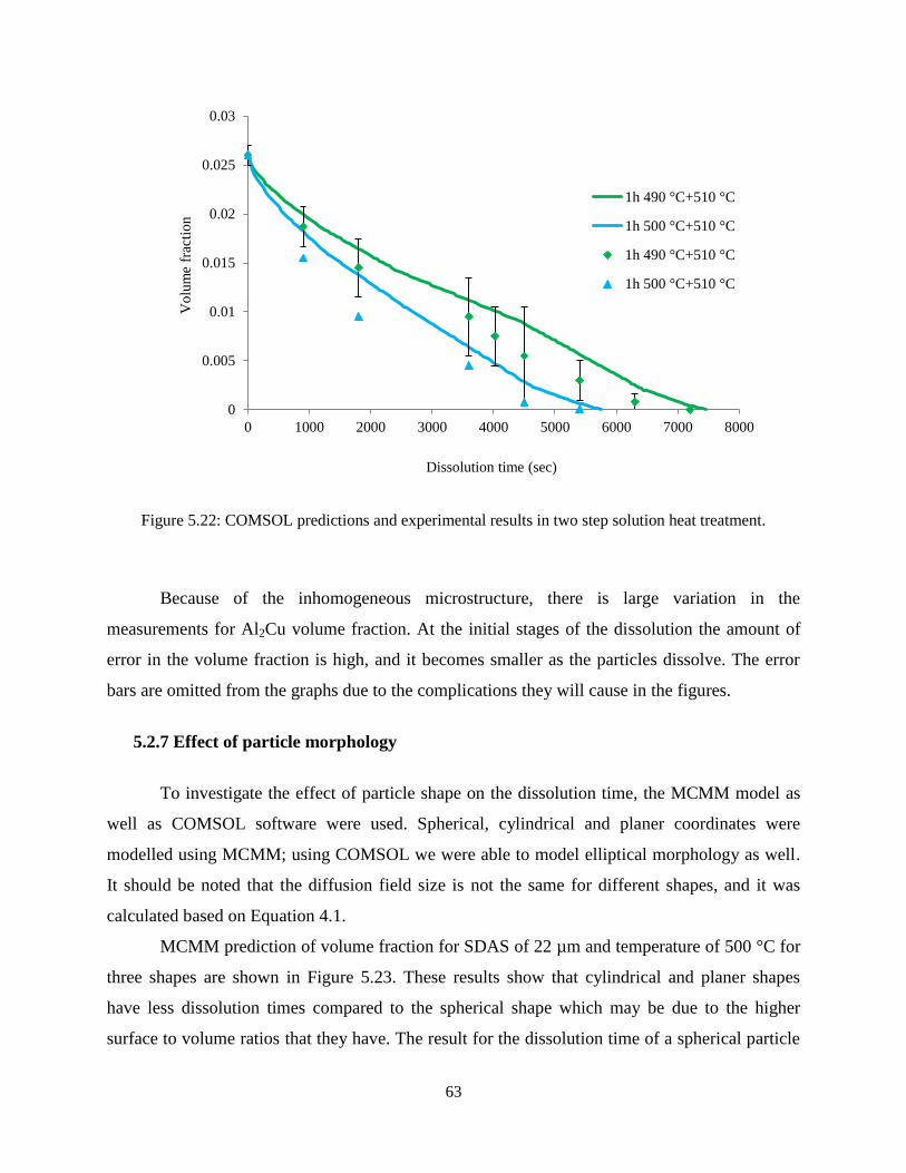
63
Figure 5.22: COMSOL predictions and experimental results in two step solution heat treatment.
Because of the inhomogeneous microstructure, there is large variation in the
measurements for Al2Cu volume fraction. At the initial stages of the dissolution the amount of
error in the volume fraction is high, and it becomes smaller as the particles dissolve. The error
bars are omitted from the graphs due to the complications they will cause in the figures.
5.2.7 Effect of particle morphology
To investigate the effect of particle shape on the dissolution time, the MCMM model as
well as COMSOL software were used. Spherical, cylindrical and planer coordinates were
modelled using MCMM; using COMSOL we were able to model elliptical morphology as well.
It should be noted that the diffusion field size is not the same for different shapes, and it was
calculated based on Equation 4.1.
MCMM prediction of volume fraction for SDAS of 22 µm and temperature of 500 °C for
three shapes are shown in Figure 5.23. These results show that cylindrical and planer shapes
have less dissolution times compared to the spherical shape which may be due to the higher
surface to volume ratios that they have. The result for the dissolution time of a spherical particle
0
0.005
0.01
0.015
0.02
0.025
0.03
0 1000 2000 3000 4000 5000 6000 7000 8000
Vo
lum
e fr
acti
on
Dissolution time (sec)
1h 490 °C+510 °C
1h 500 °C+510 °C
1h 490 °C+510 °C
1h 500 °C+510 °C

64
better fits the experimental results, which suggests that the simplification of using spherical
morphology for modelling dissolution in this alloy system was valid.
Figure 5.23: MCMM prediction of the effect of particle shape on the dissolution time.
COMSOL predictions of the dissolution of an elliptical particle with different aspect
ratios for SDAS of 22 µ and temperature of 500 °C are shown in Figure 5.24. It can be seen that
at the beginning of the dissolution process, increasing the aspect ratio decreases the dissolution
time, which could be justified by the higher surface to volume ratio at higher aspect ratio,
however, at longer dissolution times this trend changes and increasing aspect ratio, increases the
dissolution time. This is due to the fact that there is another factor affecting the dissolution time
in modelling, which is the uniformity of the diffusion of solutes. At high aspect ratios, diffusion
is less uniform at two directions in comparison to the case in which the aspect ratio is low and
the shape is close to a circle.
COMSOL prediction of the effect of morphology on the dissolution time is shown in
Figure 5.25. Same trend as in MCMM model is seen with COMSOL. Dissolution time increases
by going from planar to cylindrical and spherical to elliptical shape due to the decrease in surface
to volume ratio from planar to spherical morphology. In the case of ellipse for the aspect ratio of
3 the predicted dissolution time is somewhat similar to the spherical particle. It could be due to
0
0.002
0.004
0.006
0.008
0.01
0.012
0.014
0.016
0.018
0.02
0 500 1000 1500 2000 2500 3000 3500
Vo
lum
e F
ract
ion
Time (sec)
Spherical
Cylindrical
Planer
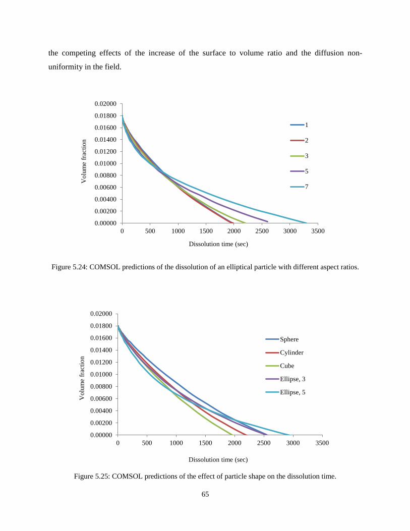
65
the competing effects of the increase of the surface to volume ratio and the diffusion non-
uniformity in the field.
Figure 5.24: COMSOL predictions of the dissolution of an elliptical particle with different aspect ratios.
Figure 5.25: COMSOL predictions of the effect of particle shape on the dissolution time.
0.00000
0.00200
0.00400
0.00600
0.00800
0.01000
0.01200
0.01400
0.01600
0.01800
0.02000
0 500 1000 1500 2000 2500 3000 3500
Vo
lum
e fr
acti
on
Dissolution time (sec)
1
2
3
5
7
0.00000
0.00200
0.00400
0.00600
0.00800
0.01000
0.01200
0.01400
0.01600
0.01800
0.02000
0 500 1000 1500 2000 2500 3000 3500
Vo
lum
e fr
acti
on
Dissolution time (sec)
Sphere
Cylinder
Cube
Ellipse, 3
Ellipse, 5

66
The COMSOL predictions of the Cu concentration gradient during the dissolution of
spherical, planar and elliptical θ phase at different times for SDAS of 22 µm and temperature
of 500 °C are shown in Figure 5.26, 5.27 and 5.28, respectively.
Figure 5.26: COMCOL prediction of the concentration Cu within the diffusion filed and radius of a
spherical particle versus time for a 2D Circle (SDAS=22 µm, temperature= 500 °C) at (a) 0, (b) 500, (c)
1500 and (d) 2100 sec.
(a) (b)
(c) (d)

67
Figure 5.27: COMCOL prediction of the concentration of Cu within the diffusion field and radius of a
planar particle versus time for a 2D Circle (SDAS=22 µm, temperature= 500 °C) at (a) 0, (b) 500, (c)
1500 and (d) 2100 sec.
(c) (d)
(a) (b)
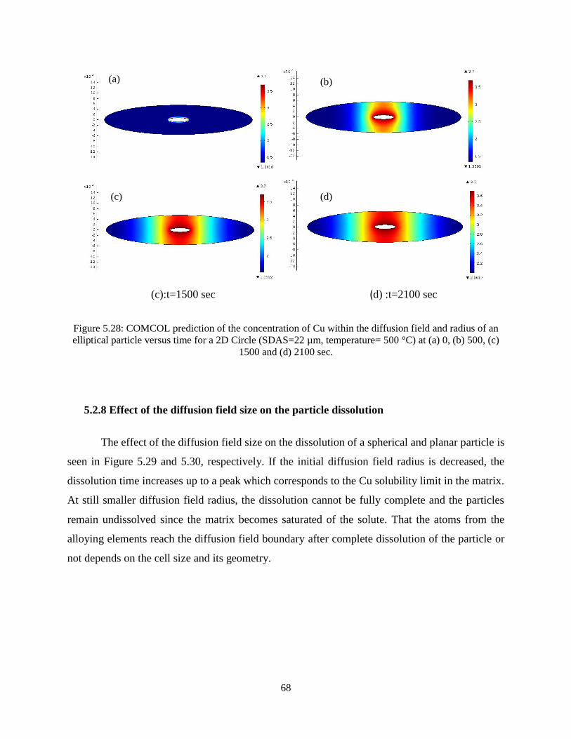
68
(c):t=1500 sec (d) :t=2100 sec
Figure 5.28: COMCOL prediction of the concentration of Cu within the diffusion field and radius of an
elliptical particle versus time for a 2D Circle (SDAS=22 µm, temperature= 500 °C) at (a) 0, (b) 500, (c)
1500 and (d) 2100 sec.
5.2.8 Effect of the diffusion field size on the particle dissolution
The effect of the diffusion field size on the dissolution of a spherical and planar particle is
seen in Figure 5.29 and 5.30, respectively. If the initial diffusion field radius is decreased, the
dissolution time increases up to a peak which corresponds to the Cu solubility limit in the matrix.
At still smaller diffusion field radius, the dissolution cannot be fully complete and the particles
remain undissolved since the matrix becomes saturated of the solute. That the atoms from the
alloying elements reach the diffusion field boundary after complete dissolution of the particle or
not depends on the cell size and its geometry.
(a) (b)
(d) (c)

69
Figure 5.29: Dissolution time for a spherical particle at different diffusion field sizes.
Figure 5.30: Dissolution time for a planar particle at different diffusion field sizes.
5.2.9 Homogenization
Now that the model has been validated, we can apply it to predict the homogenization
time. The Homogenization time—that is the time needed for complete removal of concentration
gradient within the dendrite and that the Cu concentration approaches the nominal Cu
concentration of the alloy which is 2.8—versus SDAS is shown in Figure 5.31. It can be seen
0
0.2
0.4
0.6
0.8
1
1.2
0 100 200 300 400 500
Inte
rfac
ial
Po
siti
on,
μm
Time, sec
rs = 10 μm
rs = 4 μm
rs = 2.5 μm
0
0.2
0.4
0.6
0.8
1
1.2
0 2000 4000 6000 8000 10000
Inte
rfac
ial
Po
siti
on,
μm
Time, sec
rs = 100 μm
rs = 50 μm
rs = 25 μm
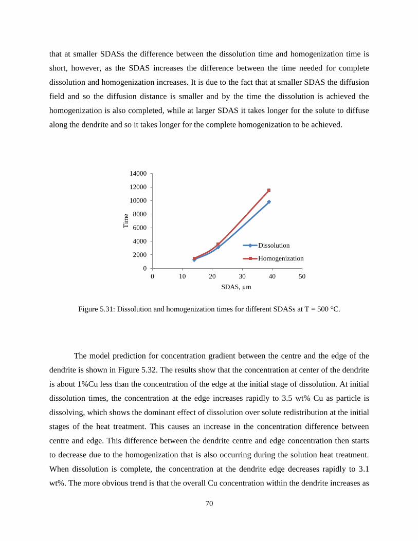
70
that at smaller SDASs the difference between the dissolution time and homogenization time is
short, however, as the SDAS increases the difference between the time needed for complete
dissolution and homogenization increases. It is due to the fact that at smaller SDAS the diffusion
field and so the diffusion distance is smaller and by the time the dissolution is achieved the
homogenization is also completed, while at larger SDAS it takes longer for the solute to diffuse
along the dendrite and so it takes longer for the complete homogenization to be achieved.
Figure 5.31: Dissolution and homogenization times for different SDASs at T = 500 °C.
The model prediction for concentration gradient between the centre and the edge of the
dendrite is shown in Figure 5.32. The results show that the concentration at center of the dendrite
is about 1%Cu less than the concentration of the edge at the initial stage of dissolution. At initial
dissolution times, the concentration at the edge increases rapidly to 3.5 wt% Cu as particle is
dissolving, which shows the dominant effect of dissolution over solute redistribution at the initial
stages of the heat treatment. This causes an increase in the concentration difference between
centre and edge. This difference between the dendrite centre and edge concentration then starts
to decrease due to the homogenization that is also occurring during the solution heat treatment.
When dissolution is complete, the concentration at the dendrite edge decreases rapidly to 3.1
wt%. The more obvious trend is that the overall Cu concentration within the dendrite increases as
0
2000
4000
6000
8000
10000
12000
14000
0 10 20 30 40 50
Tim
e
SDAS, μm
Dissolution
Homogenization

71
the Al2Cu particles are dissolving and changes from 0.5 wt% at the initial stages of solution heat
treatment up to 2.8 wt% when dissolution is complete. After the dissolution it takes 3, 8 and 28
minutes for SDASs of 14, 22 and 39 µm, respectively, that the homogenization achieve and that
the concentration reaches the nominal Cu concentration of the alloy. Such short dissolution and
homogenization times suggest that the typical 8-hour industrial solution treatments are more
likely to be dictated by ductility and toughness requirements. The latter are mainly affected by
the spherodisation and coarsening of silicon, which were not modelled in this study.
Figure 5.32: Concentration gradient along the diffusion field at T = 500 °C and for SDAS of 22 μm.
0
0.5
1
1.5
2
2.5
3
3.5
4
0 1000 2000 3000 4000
Co
nce
ntr
atio
n,
wt%
Time, sec
Field average
Dendrite
centre

72
Chapter 6
6. Conclusions and Future work
6.1 Conclusions
Dissolution of secondary phases was modelled using MATLAB and COMSOL and the
conclusion remarks are as follows:
Using MATLAB, dissolution of a single or multi component particle was modelled in
one dimension, while, COMSOL has the capability of modelling in two and three
dimensions, and the ability to model complicated geometries such as planar, cylindrical
and elliptical. However, we were not able to model dissolution of a multicomponent
phase using COMSOL as it needs the use of a user defined function to solve the equation
of the local mass conservation, which was not in the scope of this study.
It was shown that numerical modelling can be a powerful tool for gaining an
understanding of the solution treatment and homogenization behaviour of Al-Mg-Si-Cu
alloys. The numerical models presented here highlight the relative sensitivities of the
dissolution and homogenization times to SDAS and solution treatment temperature. Both
the modelling and experimental results confirm that at 500 °C dissolution is more or less
complete after 15 min, 45 min and 4 hr for SDAS of 14, 22 and 39 µm, respectively.
Dissolution times are increased by increasing SDAS or decreasing solutionizing
temperature as was expected. As image analysis revealed, the assumption made that the
particles were spaced by a SDAS was true. Hence, variation of the model predictions
from experimental results were indicative of the fact that particles do not have simple
spherical geometry and their morphology is more close to ellipsoid with aspect ratio of 7.
For the two-step solution heat treatment for SDAS of 39 µm, it was shown that solution

73
heat treatment of 1 hr 490 + 1 h 500 or 1 hr 490 °C + 30 min 510 °C can almost dissolves
all the secondary particles. After the dissolution it takes 3, 8 and 28 minutes for SDASs
of 14, 22 and 39 µm, respectively, for homogenization to achieve. Such short dissolution
and homogenization times suggest that the typical 8-hour industrial solution treatments
are more likely to be dictated by ductility and toughness requirements. The latter are
mainly affected by the spherodisation and coarsening of silicon, which were not modelled
in this study.
The effect of the morphology of the dissolving particle was also studied. It was shown
that going from planar to cylindrical to spherical and elliptical morphology, dissolution
time increases due to the decrease in surface to volume ratio. For the case of elliptical
morphology, it should be noted that there are two competing effect; one is the effect of
surface to volume ratio, and the other is the effect of uniformity of the diffusion of solute.
At the initial stages of the dissolution the effect of surface to volume ratio prevails, while
at the longer times the effect of non-uniform diffusion due to having asymmetrical
diffusion distance is predominant. Therefore, dissolution time increases compared to
spherical morphology; dissolution time increases by increasing the aspect ratio of the
ellipse.
The numerical modelling of the Q phases showed that this phase cannot be fully
dissolved at the studied temperatures for solution heat treatment, which were chosen by
the particle incipient melting restrictions. Experimental studies for the Q phase volume
fractions could not be obtained due to the very low volume fraction of the Q phase in the
studied alloy, however, modelling results were in agreement with the ThermoCalc
predictions.
6.2 Future work
The modelling homogenization process can be validated using EPMA to find the solute
concentration along the dendrite arm. EPMA can also be used to verify the solute
concentration at the particle-matrix interface.
Image analysis can be done to find the aspect ratio of the particle and the real shape of the
particle.

74
Three dimensional analysis can be done to validate the approximation of equalisation of
area fraction to volume fraction.
Experimental measurements could be done on a slightly different type of alloy with
higher amount of Mg and therefore higher amount of the Q phase to validate the accuracy
of the model in predicting concurrent dissolution of the θ and Q phases.
Model sensitivity analysis to parameters such as diffusion coefficient, activation energy,
solubility product and particle-matrix interface concentration can be done. It then should
be concluded if interdiffusion of alloying elements can be neglected or not.
A more complicated model can be developed to investigate the effect of interface
interaction in addition to the diffusion as well as the effect of unequal particle sizes in the
alloying system.
A user defined function in COMSOL for application of local mass conservation at the
interface could be developed. With this subroutine, the user can use COMSOL to predict
dissolution time for multicomponent systems.

75
7. References
[1] G. E. Totten and D. S. MacKenzie, Handbook of Aluminum: Vol. 1, Physical Metallurgy and
Processes, Ch. 1, 2003.
[2] ASM metals handbook, Vol 15, Ch. 1, 2008.
[3] I. J. Polmear: Light alloys, metallurgy of the light metals, 1980.
[4] L. Backerud, G. Chai and J. Tamminen, Solidification characteristics of aluminum alloys, Vol. 2:
Foundry alloys, Des Plains, IL, AFS/Skanaluminium, 1990.
[5] L. Arnbert, L. Backerud and G. Chai, Solidification characteristics of aluminum alloys, Vol. 3:
Dendritic coherency, Des Plains, IL, AFS, 1996
[6] A. Manente and G. Timelli, Recent Trends in Processing and Degradation of Aluminium Alloys, Ch.
9, 2011.
[7] R. Colas, A. Rodrı´guez, J. Talamantes and S. Valtierra, Solidification analysis of aluminium engine
block, International Journal of Cast Metals Research Vol. 17 No. 6, pp. 332-338, 2004.
[8] M. Schneider and C. Heisser, Modeling of microstructure and mechanical properties of aluminum
alloys during the casting and heat treatment process, AFS Proceedings, American foundary society, pp. 1-
9, 2012.
[9] A. M. Samuel, P. Ouellet, F. H. Samuel and H. W Doty, Microstructural interpretation of thermal
analysis of commercial 319 Al alloy with Mg and Sr additions, AFS Trans., Vol. 105, pp. 951-962, 1997.
[10] E. Tillová, M. Chalupová, L. Hurtalová, M. Bonek and L.A. Dobrzański, Structural analysis of heat
treated automotive cast alloy, Vol 47, issue 1, 2011.
[11] F. H. Samuel, A.M. Samuel and H. W. Doty, “Factors controlling the type and morphology of Cu-
containing phases in 319 Al alloy”, AFS Trans., Vol. 104, pp. 893-901, 1996.
[12] J. H. Sokolowski, M. B. Djurdjevic, C. A. Kierkus, D. O. Northwood, Improvement of 319
aluminum alloy casting durability by high temperature solution treatment, Journal of Materials Processing
Technology, Vol. 109, pp. 174-180, 2001.
[13] E. Tillová, M. Chalupová and L. Hurtalová, Scanning electron microscopy, Ch. 21: Evolution of
Phases in a Recycled Al-Si Cast Alloy During Solution Treatment, 2012.
76
[14] F. H. Samuel, A.M. Samuel and H. W. Doty, Factors controlling the type and morphology of Cu-
containing phases in 319 Al alloy, AFS Transactions, Vol. 104, No. 9, pp. 893-901, 1996.
[15] O. Reiso, ,H. G. Øverlie and N. Ryum, Dissolution and melting of the secondary Al2Cu phase
particles in an AlCu alloy, METALLURGICAL TRANSACTIONS A, Vol. 21A, pp. 1689-1695, 1990.
[16] I. Aguilera Luna, H. Mancha Molinar, M. J. Castro Roman, J. C. Escobedo Bocardo and M. Herrera
Trejo, Improvement of the tensile properties of an Al–Si–Cu–Mg aluminum industrial alloy by using
multi stage solution heat treatments, Materials Science & Engineering A, Vol. 561, pp. 1–6, 2013.
[17] G.Q. Wang, X.F. Bian and J. Y. Zhang, Gradual Solution Heat-Treatment of AlSiCuMg Cast Alloys,
Rare Metals, Vol. 22, pp. 304-308, 2003.
[18] A.M.A. Mohamed and F.H. Samuel, Heat Treatment - Conventional and Novel Applications, Ch.
4:A Review on the Heat Treatment of Al-Si-Cu/Mg Casting Alloys, 2012.
[19] S. Shivkumar, S. Ricci, B. Steenhoff, D. Apelian and G. Sigworth, An Experimental Study to
Optimize the Heat Treatment of A356 Alloy, AFS Transactions, Vol. 97, pp. 791-810, 1989.
[20] F. H. Samuel, “Incipient melting of Al5Mg8Si6Cu2 and Al2Cu intermetallics in unmodified and
strontium-modified Al-Si-Cu-Mg (319) alloys during solution heat treatment”, Journal of Materials
Science 33 (1998) 2283-2297.
[21] A.M.A. Mohamed, F.H. Samuel and S. Al kahtani, Influence of Mg and solution heat treatment on
the occurrence of incipient melting in Al–Si–Cu–Mg cast alloys, Materials Science and Engineering A,
Vol. 543, pp. 22– 34, 2012.
[22] F.H. Samuel, Incipient melting of Al5Mg8Si6Cu2 andAl2Cu intermetallics in unmodified and
strontium-modified Al-Si-Cu-Mg (319) alloys during solution heat treatment, JOURNAL OF
MATERIALS SCIENCE, Vol.33, pp. 2283-2297, 1998.
[23] W. Guo-hua, Z. Xiao-qin, L. Shao-guang, D. Wen-jiang and Z. Yan-ping, Effect of solution heat
treatment on the microstructure and mechanical properties of Bb319 alloy in the lost foam casting
process, Tsinghua Tongfang Knowledge Network Technology Co., Ltd.(Beijing), 2006.
[24] D. Ovono, I. Guillot and D. Massinon, The microstructure and precipitation kinetics of a cast
aluminium alloy, Scripta Materialia, Vol. 55, pp. 259–262, 2006.
[25] Z. Li, A. M. Samuel and F. H. Samuel, Effect of alloying elements on the segregation and dissolution
of CuAl2 phase in Al-Si-Cu 319 alloys, Journal of Materials Science 38, pp. 1203-1218, 2003.
[26] Y. M. Han, A. M. Samuel, F. H. Samuel and H. W. Doty, Dissolution of Al2Cu phase in non-
modified and Sr-modified 319 type alloys, International journal of Cast Metals Research, Vol. 21, No. 5,
pp. 387-393, 2008.
[27] Li, A.M. Samuel, F.H. Samuel, C. Ravindran, S. Valtierra and H.W. Doty, Factors Affecting
Dissolution of Al2Cu Phase in 319 Alloys, AFS Transactions, Vol. ΙΙΙ, pp. 03-100, pp.1-14,2003.
[28] Y. M. Han, A. M. Samuel, F. H. Samuel, S. Valtierra and H. W. Doty, Effect of solution heat
treatment type on the dissolution of copper phases in Al-Si-Cu-Mg type alloys, AFS Trans, Vol 116, pp.
79-90, 2008.
77
[29] D. Apelian, S. Shivkumar, and G. Sigworth, Fundamental Aspects-of-Heat Treatment of Cast Al-Si-
Mg Alloys,AFS Transactions, Vol. 97, pp. 727-742, 1989.
[30] Z. Li, A.M. Samuel, F. H. Samuel, C. Ravindran and S. Valtierra,Factors Affecting Dissolution of
CuAl2 Phase in 319 Alloys, Transactions of the American Foundry Society and the One Hundred Seventh
Annual Castings Congress, Milwaukee, WI; USA, pp. 26-29, 2003.
[31] Kh. A. Ragab, A.M. Samuel, A.M.A. Al-Ahmari, F.H. Samuel and H.W. Doty, Influence of
fluidized sand bed heat treatment on the performance of Al–Si cast alloys, Materials and Design, Vol. 32,
1177–1193, 2011.
[32] S.K. Chaudhury and D. Apelian, Fluidized Bed Heat Treatment of Cast Al-Si-Cu-Mg Alloys,
METALLURGICAL AND MATERIALS TRANSACTIONS A, Vol. 37A, pp. 2295-2311, 2006.
[33] G.Q. Wang, X. F. Bian and J. Y. Zhang, Gradual Solution Heat-Treatment of AlSiCuMg Cast
Alloys, Rare Metals, Vol. 22, pp. 304-308, 2003.
[34] J. Gauthier, P.R. Louchez and F. H. Samuel, Heat Treatment of 319.2 Aluminum Automotive Alloy:
Part 1, Solution Heat-Treatment, Cast Metals, Vol. 8, No.2, pp. 91-106, 1995.
[35] J. Gauthier and F. H. Samuel, Tensile Properties and Fracture Behavior of Solution Heat Treated
319.2 Aluminum Automotive Alloy, AFS Transactions, Vol. 103, pp. 849-858, 1995.
[36] H. de la Sablonnière and F. H. Samuel, Solution heat-treatment of 319 Aluminium Alloy Containing
~0.5wt% Mg Casting Alloys Part 1: Solidification and Tensile Properties, International Journal of Cast
Metals Research, Vol. 9, pp. 195-211, 1996.
[37] H. de laSablonniere and F. H. Samuel, Effect of Mg content (~0.5 wt%) and solution heat treatment
on the tensile properties of 319.1 aluminum alloy castings, Light Metals, pp. 235-245, 1996.
[38] S. N. Singh, B. P. Bardes and M. C. Flemings, Solution treatment of cast Al-4.5Cu alloy,
METALLURGICAL TRANSACTIONS, Vol. 1, pp. 1383-1388, 1970.
[39] A.M. Samuel, H.W. Doty, S. Valtierra and F.H. Samuel, Defects related to incipient melting in Al-
Si-Cu-Mg alloys, Materials and Design, Vol. 52, 947–956, 2013.
[40] S. Alkahtani, Mechanical performance of heat treated 319 alloys as a function of alloying and aging
parameters, Materials and Design, Vol. 41, pp. 358-369, 2012.
[41] A. Wiengmoon, J.T. H. Pearce, T. Chairuangsri, S. Isoda, H.Saitoe and H. Kurata, HRTEM and
HAADF-STEM of precipitates at peak ageing of cast A319 aluminium alloy, Micron, Vol. 45, 32–36,
2013.
[42] P. Apichai1, J. Kajornchiyakul, J.T.H. Pearce and A. Wiengmoon, Effect of Precipitation Hardening
Temperatures and Times on Microstructure, Hardness and Tensile Properties of Cast Aluminium Alloy
A319, vol. 143-144,pp. 306-310, 2003.
[43] H.K. Kang, M. Kida and H. Miyahara, Age hardening characteristics of Al-Si-Cu-Base cast alloys,
AFS Trans, Vol. 107, 507-515, 1999.

78
[44] M. Abdulwahaba, I.A. Madugua, S.A. Yaroa, S.B. Hassana and A.P.I. Popoola, Effects of multiple-
step thermal ageing treatment on the hardness characteristics of A356.0-type Al–Si–Mg alloy, Materials
and Design, Vol. 32,pp. 1159–1166, 2011.
[45] E. Sjölander and S. Seifeddine, The heat treatment of Al–Si–Cu–Mg casting alloys, Journal of
Materials Processing Technology, Vol.210, 1249–1259, 2010.
[46] H.B. Aaron, On the kinetics of precipitate dissolution, Metal science journal, Vol. 2, pp. 192-193,
1968.
[47] M. J. Whelan, On the kinetics of precipitate dissolution Metal Science Journal, Vol. 3, pp. 95-97,
1969.
[48] H. B. Aaron and G. R. Kotler, Second phase dissolution, Metallurgical transactions, Vol. 2, pp. 393-
408, 1971.
[49] U. H. Tundal and N. Ryum, Dissolution of particles in binary alloys: Part 1: computer simulation,
Metallurgical transactions A, Volume 23A, pp. 433-444, 1992.
[50] G. Thomas and M. J. Whelan, Observation of precipitation in thin foils of Aluminum +4% copper
alloy, Philosophical Magazine, Vol. 6, 1103-1114, 1961.
[51] F. V. Nolfi, P. G. Shewmon, and J. S. Foster, The dissolution and growth kinetics of spherical
precipitates, Transactions of the metallurgical society of AIME, Vol. 245, pp. 1427-1433, 1969.
[52] L. C. Brown, Diffusion-controlled dissolution of planar, cylindrical, and spherical precipitates,
Journal of Applied Physics, Vol. 47, No. 2, 1976.
[53] V. V. Teleshov and V. S. Zolotorevsky, Tsvetnaya Met., Vol. 5, pp. 136-141, 1967.
[54] P.A. Rometsch, L. Arnberg and D. L. Zhang, Modelling dissolution of Mg2Si and homogenisation in
Al-Si-Mg alloys, International Journal of Cast Metals, Vol. 12, pp. 1-8, 1999.
[55] E. Javierre, C. Vuik, F.J. Vermolen and S. van der Zwaag, A comparison of numerical models for
one-dimensional Stefan problems, Journal of Computational and Applied Mathematics, Vol. 192, pp 445–
459, 2006.
[56] C. Vuik, A. Segal and F.J. Vermolen, A conserving discretization for a Stefan problem with an
interface reaction at the free boundary, Computer Visual Science, Vol. 3, pp. 109–114, 2000.
[57] G. Segal, K.Vuik, and F. J. Vermolen, A Conserving Discretization for the Free Boundary in a Two-
Dimensional Stefan Problem, JOURNAL OF COMPUTATIONAL PHYSICS, Vol. 141, pp. 1–21, 1998.
[58] E. Javierre, C. Vuik, F.J. Vermolen and A. Segal, A level set method for three dimensional vector
Stefan problems: Dissolution of stoichiometric particles in multi-component alloys, Journal of
Computational Physics, Vol. 224, pp. 222–240, 2007.
[59] F. Vermolen, K. Vuik and S. van der Zwaag, A mathematical model for the dissolution kinetics of
Mg2Si-phases in Al–Mg–Si alloys during homogenisation under industrial conditions, Materials Science
and Engineering A, Vol. 254,pp.13–32, 1998.

79
[60] F.J. Vermolen and C. Vuik, A mathematical model for the dissolution of particles in multi-
component alloys, Journal of Computational and Applied Mathematics, Vol. 126, pp. 233-254, 2000.
[61] F.J. Vermolen, C. Vuik and S. van der Zwaag, A mathematical model for the dissolution of
stoichiometric particles in multi-component alloys, Materials Science and Engineering A, Vol. 328, pp.
14–25, 2002.
[62] F. J.Vermolen, K. Vuik and S. van der Zwaag, A numerical analysis for the dissolution of second
phase particles in ternary alloys, Moving boundaries IV - Computational modelling of free and moving
boundary problems, pp. 153-162, (1997).
[63] F. J.Vermolen, K. Vuik and S.van der Zwaag, The dissolution of a stoichiometric second phase in
ternary alloys: a numerical analysis, Materials Science and Engineering A, Vol. 246, pp. 93–103, 1998.
[64] F. J.Vermolen and K.Vuik, A numerical method to compute the dissolution of second phases in
ternary alloys, Journal of computational and applied mathematics, Vol. 93, pp. 123-143, 1998.
[65] F.J. Vermolen, P. Pinson, C. Vuik and S. van der Zwaag, A suite of sharp interface models for solid-
state transformations in alloys, European Conference on Computational Fluid Dynamics ECCOMAS
CFD, 2006.
[66] F.J. Vermolen, E. Javierre, C. Vuik, L. Zhao and S. van der Zwaag, A three-dimensional model for
particle dissolution in binary alloys Computational Materials Science, Vol. 39, pp. 767–774, 2007.
[67] F.J. Vermolen, C. Vuik and S. van der Zwaag, Cross-diffusion controlled particle dissolution in
metallic alloys, Comput Visual Sci, Vol. 8, pp. 27–33, 2005.
[68] F.J. Vermolen, C. Vuik and S. van der Zwaag, Particle dissolution and cross-diffusion in multi-
component alloys, Materials Science and Engineering A, Vol. 347, 265-279, 2003.
[69] F. J. Vermolen and S. van der Zwaag, A numerical model for the dissolution of spherical particles in
binary alloys under mixed mode control, Materials Science and Engineering A, Vol. 220, pp. 140-146,
1996.
[70] F. J. Vermolen, P. van Mourik and S. van der Zwaag, Analytical approach to particle dissolution in a
finite medium, Materials Science and Technology, Vol. 13, 308-312, 1997.
[71] F. J. Vermolen, H. M. Slabbekoorn and S. van der Zwaag, The apparent activation energy for the
dissolution of spherical Si-particles in AlSi-alloys, Materials Science and Engineering A, Vol. 231, pp 80-
89, 1997.
[72] E. Sjölander and S. Seifeddine, Optimisation of solution treatment of cast Al–Si–Cu alloys, Materials
and Design, Vol. 31, pp. 44–S49, 2010.
[73] E. Sjölander, Heat treatment of Al-Si-Cu-Mg casting alloys, P.hD. thesis, 2011.
[74] L. J. Colley, Microstructure-property models for T6 heat treatment of Al-Si-Mg alloys, P.hD. thesis,
2010.
[75] M. Mantina, Y. Wang, R. Arroyave, C. Wolverton, L. Q. Chen and Z. K. Liu, Phys Rev Lett., Vol.
100, 215901, 2008.

80
[76] N.A. Belov, D. G. Eskin and A.A. Aksenov, Multicomponent phase diagrams: applications for
commercial aluminum alloys, Elsevier,1st edition, 2005.
[77] N.A. Belov, A.A. Aksenov and D. G. Eskin, Iron in Aluminium Alloys: Impurity and Alloying
Element, Taylor and Francis 2002.
[78] L. Arnberg and B. Aurivillius, The Crystal Structure of AlxCu2Mg12-xSi7, (h-AlCuMgSi), Acta
Chemica Scandinavica A, Vol. 34, pp. 1-5, 1980.
[79] S. Seifeddine, E. Sjölander and T. Bogdanoff, On the Role of Copper and Cooling Rates on the
Microstructure, Defect Formations and Mechanical Properties of Al-Si-Mg Alloys, Materials Sciences
and Applications, Vol. 4, pp. 171-178, 2013.
[80] S. P. Nikanorov, M. P. Volkov, V.N. Gurin, Yu. A. Burenkov, L. I. Derkachenka, B.K. Kardashev,
L. L. Regel and W.R. Wilcox, Structural and mechanical properties of Al–Si alloys obtained by fast
cooling of a levitated melt, Materials Science and Engineering A, Vol. 390, pp. 63-69, 2005.
[81] M. Gupta and S. Ling, Microstructure and mechanical properties of hypo/hypereutectic Al–Si alloys
synthesized using a near-net shape forming technique, Journal of Alloys and Compounds, Vol. 287, pp.
284-294, 1999.
[82] J. Zhang, Y. N. Huang, C. Mao nad P. Peng, Structural, elastic and electronic properties of y (Al2Cu)
and S(Al2CuMg) strengthening precipitates in Al–Cu–Mg series alloys: First-principles calculations,
Solid State Communications, Vol. 152, pp. 2100–2104, 2012.
[83] M. Voncina, J. Medved, T. Boncina and F. Zupanic, Effect of Ce on morphology of α(Al)−Al2Cu
eutectic in Al−Si−Cu alloy, Trans. Nonferrous Met.Soc. China, Vol. 24, pp. 36−41, 2014.
[84] X. M. Pan, C. Lin, J. E. Morral and H.D. Brody, An Assessment of Thermodynamic Data for the
Liquid Phase in the Al-Rich Corner of the Al-Cu-Si System and Its Application to the Solidification of a
319 Alloy, Journal of Phase Equilibria and Diffusion, Vol. 26, No. 3, 2005.
[85] C. Wolverton, Crystal structure and stability of complex precipitate phases in Al-Cu-Mg-(Si) and Al-
Zn-Mg alloys, Acta Materialia, Vol. 49, pp. 3129–3142, 2001.
[86] C. Ravi, C. Wolverton, First-principles study of crystal structure and stability of Al–Mg–Si–(Cu)
precipitates, Acta Materialia, Vol. 52, 4213–4227, 2004.
[87] H. Fredriksson, U. Åkerlind, Solidification and Crystallization Processing in Metals and Alloys,
Wiley, 2012.
[88] L. Liu, A.M.A. Mohamed, A.M. Samuel, F.H. Samuel, H.W. Doty, and S. Valtierra, Precipitation of
β-Al5FeSi Phase Platelets in Al-Si Based Casting Alloys, METALLURGICAL AND MATERIALS
TRANSACTIONS A, Vol. 40A, pp. 2457-2469, 2009.
[89] R. I. Mackay, J. H. Sokolowski, Effect of Si and Cu concentrations and solidification rate on
soundness in casting structure in Al–Si–Cu alloys, International Journal of Cast Metals Research, Vol. 23
No. 1, pp. 7-22, 2010.

81
[90] N. C. W. Kuijpers, F. J. Vermolen, K. Vuik, S. van der Zwaag, A Model of the -AlFeSi to α-
Al(FeMn)Si Transformation During Homogenization in 6xxx Alloys, Materials Transactions, Vol. 44,
No. 7, pp. 1448-1456, 2003.

82
Appendices
A: Numerical discretization
Stationary interface
Discretization of the equations 4.8 and 4.9 is as follows:
𝑚𝑖𝑛 = 𝐷(𝑐𝑖−1 − 𝑐𝑖)𝜌
𝑑𝑟4𝜋𝑟𝑖−1
2𝑡
𝑚𝑜𝑢𝑡 = 𝐷(𝑐𝑖 − 𝑐𝑖+1)𝜌
𝑑𝑟4𝜋𝑟𝑖
2𝑡
And the solute concentration added to each shell after each time step can be obtained as follow;
𝑐𝑖 =𝑚𝑎𝑠𝑠 𝑎𝑑𝑑𝑒𝑑 𝑡𝑜 𝑠ℎ𝑒𝑙𝑙
𝑣𝑜𝑙𝑢𝑚𝑒 𝑜𝑓 𝑡ℎ𝑒 𝑠ℎ𝑒𝑙𝑙= (𝑚𝑖𝑛
𝑖 −𝑚𝑜𝑢𝑡𝑖 ) 𝜌⁄
4𝜋3⁄ (𝑟𝑖
3 − 𝑟𝑖−13 )
(𝐴. 1)
Concentration after each time step can then be calculated as follow;
𝑐𝑖𝑡+1 = 𝑐𝑖
𝑡 + 𝑐𝑖
𝑐𝑖𝑡+1 = 𝑐𝑖
𝑡 + 3𝑟𝑖−12 (𝑐𝑖−1 − 𝑐𝑖) − 𝑟𝑖
2(𝑐𝑖 − 𝑐𝑖+1)
(𝑟𝑖3 − 𝑟𝑖−1
3 ) (𝐴. 2)

83
Moving boundary
Discretization of the interior region
An implicit finite difference method is used to solve the diffusion equation. Since the
magnitude of the gradient is maximal near the moving interface we use a geometrically
distributed grid such that the discretization near the interface is fine and coarse farther away from
the moving interface. Furthermore, a virtual grid-point near the moving boundary is used. The
distance between the virtual node and the interface is chosen equal to the distance between the
interface and the first grid-node.
Discrete boundary conditions at the interface
The discrete approximation of the concentration is defined as𝑐𝑖,𝑘𝑗
, where j, i and k
respectivelydenote the time-step, the index of the chemical (alloying) element and grid-node.
The virtual grid-node behind the moving interface and the grid-node at the interface respectively
have indices k = -1 and k = 0. At the moving interface, it is obtained from discretization of
Equation (4.21)
𝐷𝐶𝑢
𝑐𝐶𝑢𝑝 − 𝑐𝐶𝑢
𝑠𝑜𝑙
𝑐𝐶𝑢,1𝑗+1
− 𝑐𝐶𝑢,−1𝑗+1
2∆𝑟=
𝐷𝑆𝑖
𝑐𝑆𝑖𝑝 − 𝑐𝑆𝑖
𝑠𝑜𝑙
𝑐𝑆𝑖,1𝑗+1
− 𝑐𝑆𝑖,−1𝑗+1
2∆𝑟
𝐷𝐶𝑢
𝑐𝐶𝑢𝑝 − 𝑐𝐶𝑢
𝑠𝑜𝑙
𝑐𝐶𝑢,1𝑗+1
− 𝑐𝐶𝑢,−1𝑗+1
2∆𝑟=
𝐷𝑀𝑔
𝑐𝑀𝑔𝑝 − 𝑐𝑀𝑔
𝑠𝑜𝑙
𝑐𝑀𝑔,1𝑗+1
− 𝑐𝑀𝑔,−1𝑗+1
2∆𝑟
The concentration profile of each element is determined by the value of the interfacial
concentration. Above equations can be re-arranged into a zero-point equations for all chemical
elements. All interfacial concentrations satisfy the hyperbolic equation (4.13). Combination of all
equations give:
𝐷𝐶𝑢(𝑐𝐶𝑢,1𝑗+1
− 𝑐𝐶𝑢,−1𝑗+1
)(𝑐𝑆𝑖𝑝 − 𝑐𝑆𝑖
𝑠𝑜𝑙) − 𝐷𝑆𝑖(𝑐𝑆𝑖,1𝑗+1
− 𝑐𝑆𝑖,−1𝑗+1
)(𝑐𝐶𝑢𝑝 − 𝑐𝐶𝑢
𝑠𝑜𝑙) = 0
𝐷𝐶𝑢(𝑐𝐶𝑢,1𝑗+1
− 𝑐𝐶𝑢,−1𝑗+1
)(𝑐𝑀𝑔𝑝 − 𝑐𝑀𝑔
𝑠𝑜𝑙) − 𝐷𝑆𝑖(𝑐𝑀𝑔,1𝑗+1
− 𝑐𝑀𝑔,−1𝑗+1
)(𝑐𝐶𝑢𝑝 − 𝑐𝐶𝑢
𝑠𝑜𝑙) = 0

84
(𝑐1𝑠𝑜𝑙)
𝑚1(𝑐2𝑠𝑜𝑙)
𝑚𝑛(… )(𝑐𝑛𝑠𝑜𝑙)𝑚𝑛 − 𝐾𝑠𝑜𝑙 = 0
Diffusion equation needs to be solved for every component in the system. In the case of a
moving boundary we do not know the value of 𝑐𝑖𝑠𝑜𝑙. We need equations (4.13) and (4.17) to
determine this value. Because this is a nonlinear problem we proceed as follows.
1. Take a good first guess for𝑐𝑖,𝑠𝑜𝑙𝑗+1
.
2. Using the current estimate for 𝑐𝑖,𝑠𝑜𝑙𝑗+1
and 𝑅𝑘𝑗+1
, and the 𝑐𝑖𝑗 and 𝑅𝑘
𝑗 from the previous
time step, we can calculate the new concentration profiles of each component, as well
as the concentration gradient at the boundaries.
3. Now we have enough information to do a Newton-Raphson step to obtain a better
approximation for 𝑐𝑖,𝑠𝑜𝑙𝑗+1
.
4. Continue with step 1 until the desired accuracy is reached.
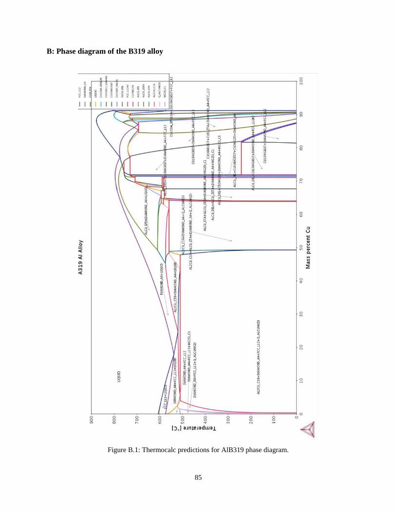
85
B: Phase diagram of the B319 alloy
Figure B.1: Thermocalc predictions for AlB319 phase diagram.

86
C: FactSage result
Figure C.1: FactSage prediction for phase diagram of AlB319.

87
D: Analytical validation of the model via Vermolen model
The model predictions were validated using Vermolen results [61].
Table D.1: Input data.
Figure D.1: The interfacial position as a function of time for a planar dissolving particle; a) Vermolen
model and b) model of this study.
0.00E+00
2.00E-07
4.00E-07
6.00E-07
8.00E-07
1.00E-06
1.20E-06
0 5000 10000 15000
Inte
rfac
ial
po
siti
on
Time (s)
Case I
Case II
Case III
Case IV

88
Figure D.2: The interfacial position as a function of time for a planar dissolving particle; a) Vermolen
model and b) model of this study.
Figure D.3: The interfacial position as a function of time for a spherical dissolving particle; a) Vermolen
model and b) model of this study.
0.00E+00
2.00E-07
4.00E-07
6.00E-07
8.00E-07
1.00E-06
1.20E-06
0 5000 10000
Inte
rfac
ial
po
siti
on (
um
)
Time (s)
Case III
Case III-rs5e-5
Case III-rs2.5e-5
0.00E+00
2.00E-07
4.00E-07
6.00E-07
8.00E-07
1.00E-06
1.20E-06
0 100 200 300
Inte
rfac
ial
po
siti
on (
um
)
Time (s)
Case I
Case II
Case III
Case IV

89
Figure D.4: The interfacial posision as a function of time for a spherical dissolving particle; a)
Vermolen model and b) model of this study.
0.00E+00
2.00E-07
4.00E-07
6.00E-07
8.00E-07
1.00E-06
1.20E-06
0 200 400 600
Inte
rfac
ial
po
siti
on (
m)
Time (s)
Case I
Case I-rs4e-6
Case I-rs2.5e-6
Copyright © 2022 FDOKUMEN