1

Modelling Dam-break Flows over Mobile Beds using a 2D Coupled Approach 1

Junqiang Xia1,2, Binliang Lin1, Roger A. Falconer1, and Guangqian Wang2 2

(1 Hydro-environmental Research Centre, School of Engineering, Cardiff University, CF24 3AA, UK) 3

(2 State Key Laboratory of Hydroscience and Engineering, Tsinghua University, Beijing 100084, China) 4

5

Abstract: Dam-break flows usually propagate along rivers and floodplains, where the processes 6

of fluid flow, sediment transport and bed evolution are closely linked. However, the majority of 7

existing two-dimensional (2D) models used to simulate dam-break flows are only applicable to 8

fixed beds. Details are given in this paper of the development of a 2D morphodynamic model for 9

predicting dam-break flows over mobile beds. In this model, the common 2D shallow water 10

equations are modified, so that the effects of sediment concentrations and bed evolution on the 11

flood wave propagation can be considered. These equations are used together with the 12

non-equilibrium transport equations for graded sediments and the equation of bed evolution. The 13

governing equations are solved using a matrix method, thus the hydrodynamic, sediment transport 14

and morphological processes can be jointly solved. The model employs an unstructured finite 15

volume algorithm, with an approximate Riemann solver, based on the Roe-MUSCL scheme. A 16

predictor-corrector scheme is used in time stepping, leading to a second-order accurate solution in 17

both time and space. In addition, the model considers the adjustment process of bed material 18

composition during the morphological evolution process. The model was first verified against 19

results from existing numerical models and laboratory experiments. It was then used to simulate 20

dam-break flows over a fixed bed and a mobile bed to examine the differences in the predicted 21

flood wave speed and depth. The effects of bed material size distributions on the flood flow and bed 22

evolution were also investigated. The results indicate that there is a great difference between the 23

2

dam-break flow predictions made over a fixed bed and a mobile bed. At the initial stage of a 1

dam-break flow, the rate of bed evolution could be comparable to that of water depth change. 2

Therefore, it is often necessary to employ the turbid water governing equations using a coupled 3

approach for simulating dam-break flows. 4

Keyword: morphodynamic model, dam-break flows, mobile bed, coupled solution, finite volume 5

method 6

1 Introduction 7

Dam-break flows could lead to severe flooding with catastrophic consequences, such as damage 8

to properties and loss of human life. Therefore, dam-break flows have been the subject of 9

scientific and technical research for many hydraulic scientists and engineers. Earlier studies 10

were primarily based on analytical solutions for idealised conditions. For example, Stoker [1] 11

developed an analytical solution to predict dam-break flows in an idealised channel, in which 12

the bed slope was assumed to be zero and the friction term was ignored. Chanson [2] proposed 13

an analytical solution of dam-break waves with flow resistance, and then it was applied to 14

simulate tsunami surges on dry coastal plains. During the past two decades, numerical models and 15

laboratory experiments have become very popular for investigating dam-break flows [3-7]. With the 16

advancement of computer technology and numerical solution methods of the shallow water 17

equations, hydrodynamic models based on one-dimensional (1D) and two-dimensional (2D) 18

approaches are increasingly being used for predicting dam-break flows. Currently, numerical 19

solutions of the shallow water equations type are one of the most active topics in the field of 20

hydraulics research. Several numerical models pertaining to dam-break flows can be found in the 21

literature, and they have been successfully used to predict flood inundation extent and velocity 22

distributions. However, the majority of these models are only applicable to dam-break flows over 23

3

fixed beds [3, 8-11]. In some catastrophic flood events, particularly those caused by dam or dike 1

failures, flood flows have induced severe sediment movements in various forms: debris flows, mud 2

flows, floating debris and sediment-laden currents [12]. Capart et al. [13] pointed out that in some 3

extreme cases, the volume of entrained material could reach the same order of magnitude as the 4

volume of water initially released from the failed dam. For example, the Chandora river dam-break 5

flow occurred in India in 1991 scoured a 2 m thick layer of bed material from the reach immediately 6

downstream of the dam [14]. It is often necessary to account for the process of morphological 7

changes when simulating such severe dam-break flows. Currently, two approaches are often used to 8

model the morphodynamic processes: uncoupled and coupled solutions [15]. In order to model the 9

morphodynamic processes caused by dam-break flows, the second method may be more acceptable. 10

This is due to the rate of bed evolution often being more comparable to the rate of water depth 11

variation. Early numerical models for simulating dam-break flows over mobile beds often adopted 12

uncoupled solutions that did not account for the effects of sediment transport and bed deformation 13

on the movement of flow [4, 16-17]. Fraccarollo and Capart [18], Spinewine and Zech [19] used 14

two-layer 1D models to simulate dam-break flows over mobile beds. These models were applicable 15

to morphological changes caused predominately by the non-equilibrium transport of bed load. The 16

applicability of the models was considered to be limited because of the assumption of a constant 17

sediment concentration in the lower layer [6]. More recently, several models for simulating 18

dam-break flows over mobile beds based on the coupled solution have been developed. Cao et al. 19

[20] presented a 1D numerical model to simulate the hydraulics of dam-break flows over mobile 20

beds and the induced sediment transport and morphological evolution, and provided a detailed 21

description of dam-break fluvial processes. Recently they extended the analysis of the multiple time 22

scales of subaerial (near-bed) sediment-laden flows over erodible bed to subaqueous turbidity 23

4

currents, and proposed a fully coupled modelling study [21-22]. Wu and Wang [6] proposed a 1

similar 1D model to simulate dam-break flows over mobile beds using the coupled solution, and 2

applied the model to investigate the mechanisms of morphodynamic processes caused by dam-break 3

flows. In Wu and Wang’s model, a more complex method was used to calculate the rates of 4

sediment deposition and entrainment, which could account simultaneously for the process of bed 5

evolution caused by the suspended and bed loads. 6

Although many 2D dam-break flow models over non-mobile or fixed beds have been 7

developed over the past decade [3,5,8-11,23-24], 2D models for dam-break flows over mobile beds 8

using the coupled solution are not often reported due to the complexity of flow-sediment transport 9

and bed evolution. Simpson and Castelltort [25] extended an existing 1D coupled model of Cao et 10

al. [20] to a 2D model for the free surface flow, sediment transport and morphological evolution. 11

This model used a Godunov-type method with a first-order approximate Riemann solver, and was 12

verified by comparing the computed results with the documented solutions. As commented by Cao 13

[26], the first-order numerical scheme in solving the governing equations may have limitations in 14

modelling water levels and sediment concentrations with gradient discontinuities. The model was 15

applied to test cases with some idealized flat bed channels, without the need to consider the wetting 16

and drying fronts. Therefore, it is necessary to develop a morphodynamic model for simulating 17

dam-break flows over mobile beds with more advanced solution schemes and wider applicability. 18

In the current study, a 2D morphodynamic model has been developed to simulate dam-break 19

flows over mobile beds. In the model, a 2D hydrodynamic module is coupled with the sediment 20

transport and bed evolution modules to predict simultaneously the hydrodynamics, sediment 21

concentrations and morphological changes. The model was first verified against results from 22

existing numerical models and experimental data from laboratory tests documented in the literature, 23

5

and was then used to investigate the influences of different bed material compositions on the flood 1

levels and the morphology of channel bed. Finally, this study simulated dam-break flows over a 2

fixed bed and a mobile bed to examine the differences in the predicted flood wave speed and depth. 3

2 Governing equations 4

Due to the interaction between the sediment-laden flow and river bed, a river will undergo 5

continuous morphological changes. For dam-break flows, the processes of flood wave propagation 6

and river channel evolution will usually be very significant. In order to accurately model these 7

processes, the following equations are used in the current model: 8

(i) a set of modified shallow water equations, which are able to take into account the influences of 9

sediment transport and bed deformation on the flood flows; 10

(ii) the non-equilibrium transport equations for both suspended and bed loads; and 11

(iii) the equation of bed evolution. 12

In this study, graded sediments are considered, with a computational procedure being employed to 13

allow bed-material composition adjustment to be made. 14

2.1 Hydrodynamic equations 15

The hydrodynamic governing equations used are based on the two-dimensional shallow water 16

equations, but with additional terms being included to account for the sediment effects on the fluid 17

density and bed level change [15, 27]. The shallow water governing equations of the 2D 18

hydrodynamic model comprise the mass and momentum conservation equations for the 19

water-sediment mixture flow. Coupled equations have been presented in a one-dimensional form by 20

Fagherazzi and Sun [4] and Cao et al. [20], and in a two-dimensional form by Simpson and 21

Castelltort [25], Yue and Cao et al. [28]. The modified continuity (Eq. (1)) and momentum 22

6

equations in the x and y directions (Eqs. (2) and (3)) can be expressed in detail as follows: 1

( ) ( ) ( ) bZh hu hv

t x y t

(1) 2

2 2 22 2 01

2 2 2( ) ( ) ( ) ( ) ( )

2m b

bx fx ts m m

u Zu u gh Shu hu gh huv gh S S hv

t x y x y x t

(2) 3

2 2 22 2 01

2 2 2( ) ( ) ( ) ( ) ( )

2m b

by fy tm s m

v Zv v gh Shv huv hv gh gh S S hv

t x y x y y t

(3) 4

in which t = time; h = water depth; u and v = velocity components in the x and y 5

directions, respectively; g = gravitational acceleration; t = turbulent viscosity coefficient, 6

*t u h , where *u = friction velocity and = empirical coefficient, 0.0 1.0 ; 7

s f , in which f = clear water density and s = sediment density; m = density of 8

water-sediment mixture, m = (1 )v f v sS S , where vS is the volumetric sediment 9

concentration, and /v sS S , in which S = total concentration of graded sediments; 0 = 10

density of saturated bed material, 0 = (1 / )s f , in which = dry density of bed 11

material. The bed slope terms ( bxS , byS ) and friction slope terms ( fxS , fyS ) are written as 12

/bx bS Z x , /by bS Z y and 2 2 2 4/3/fxS n u u v h , 2 2 2 4 /3/fyS n v u v h , in the x , 13

y directions, respectively, where bZ = bed elevation; n = Manning’s roughness coefficient. 14

The last two terms on the right-hand side of Eqs. (2) and (3) represent respectively, spatial 15

variations in sediment concentration, and momentum transfer due to sediment exchange between 16

the flow and the erodible bed. These two terms are only significant during the transport of 17

hyper-concentrated flows or during the rapid bed evolution, and they seldom appear in the classical 18

clear-water governing equations. 19

2.2 Transport equations of suspended and bed loads 20

In the current model, the non-equilibrium transport processes of graded suspended and bed 21

7

loads are included in the equation of sediment transport. 1

For the suspended load, the 2D non-equilibrium transport equation is given as: 2

*( ) ( ) ( ) ( ) ( ) ( )k kk k k s s sk sk k k

S ShS huS hvS h h S S

t x y x x y y

(4-1) 3

in which s = turbulent diffusion coefficient of sediment; subscript k represents the kth sediment 4

fraction; kS , *kS , and sk represent, respectively, the sediment concentration, sediment transport 5

capacity and effective settling velocity for the kth fraction; sk = non-equilibrium adaptation 6

coefficient of suspended load, which is an empirical coefficient associated with the rate of bed 7

evolution. 8

Several empirical methods have been proposed in the literature for determining the value of 9

sk , with significant differences existing among these methods [20,29]. It has been found that if the 10

same sk value is used for all of the sediment fractions, then during the process of bed degradation 11

the amount of coarse sediment eroded from the bed is greater than that of the finer fraction. This 12

causes the composition of bed material to become finer, rather than getting coarser, which is 13

physically incorrect. In order to avoid this, different values of sk are usually set for different 14

fractions. In the present study, the following empirical formulae were used to determine sk [30]: 15

0.3/sk sk , when *k kS S , and 16

0.7/sk sk , when *k kS S , 17

in which is a case-dependent coefficient. 18

For the bed load, the 2D non-equilibrium transport equation proposed by Dou et al. [31] is 19

used, given as: 20

*( ) ( ) ( ) ( )bk bk bk bk bk bk b khq huq hvq q qt x y

(4-2) 21

in which bkq = amount of bed load in a unit volume of water, in kg/m3; bk = setting velocity of 22

8

bed load; *b kq = transport capacity of bed load in a unit volume of water, in kg/m3; and bk = 1

non-equilibrium adaptation coefficient of bed load. Several studies have been conducted to 2

determine this coefficient [31-32]. In the current study, the value of bk suggested by Dou et al. 3

[31] was used, and it ranged from 0.1 to 1.0. 4

2.3 Bed evolution equations 5

The equation used to represent the suspended load induced during bed evolution is written as: 6

*( )sksk sk k k

ZS S

t

(5-1) 7

The equation used to represent the bed load induced during bed evolution is written as: 8

*( )bkbk bk bk b k

Zq q

t

(5-2) 9

Therefore, the thickness of the channel bed due to the total sediment load is given as: 10

t1 1

s

s

N N

sk bkk k N

Z Z Z

(5-3) 11

in which N = total number of fractions of non-uniform sediments; sN = number of fractions of 12

non-uniform suspended sediments; skZ and bkZ = thicknesses of bed deformation caused by 13

suspended load and bed load, respectively, in one time step; and tZ = total thickness of bed 14

evolution in one time step. Therefore, the bed elevation at a cell after one time step can be obtained 15

by 1t(Z ) (Z )l l

b b Z , in which the superscript l represents the time level. 16

2.4 Sediment transport capacity 17

A formula proposed by Wu and Long [33] is used to compute the sediment transport capacity 18

of the suspended load, which is given as: 19

3

* [ ]Mm

s m m

US K

gh

(6) 20

where K and M are two empirical parameters, K = 0.452 kg/m3 and M = 0.762; U = 21

9

depth-average speed, 2 2U u v ; s and m = specific weights of sediment and turbid 1

water; m = group settling velocity of graded suspended sediments, m = 1/*

1

( )sN

M Mk sk

k

P

; 2

kP* = percentage of sediment transport capacity for the kth size fraction, which is determined 3

using *1

( / ) / ( / )sN

k bk sk bk skk

P P P

, in which is an empirical coefficient, and bkP = 4

percentage of bed material for the kth grain size fraction. 5

A formula proposed by Dou et al. [31] is used to determine the bed load transport capacity, 6

which is given as: 7

3

0 20

( )b s mb k ck bk

s m bk

K Uq U U P

C g

(7) 8

in which 0b kq = bed load transport capacity per unit width for the kth grain size fraction in kg/m.s; 9

bK is an empirical coefficient; ckU = incipient velocity of the kth bed load fraction; 0C = 10

dimensionless Chézy coefficient with 0 /C C g , in which 1/ 6 /C h n . The value of bed load in 11

a unit volume is obtained according to * 0 /b k b kq q hU . This formula can be used to compute the 12

transport capacity of sand or gravel bed-load whose diameter ranges from 0.05 to 200 mm. The 13

value of parameter bK in Eq. (7) was calibrated by the experimental data and it was about 0.1. 14

2.5 Bed material composition adjustment during bed evolution 15

In order to simulate the phenomenon of armoring, i.e. sorting of bed material, caused by 16

degradation or aggradation, the bed material at each computational cell is divided into two vertical 17

layers: the upper one is called the mixing or active layer and the lower one is called the memory 18

layer. The thickness of the mixing layer is denoted by bH , with its gradation being represented by 19

bkP . The memory layer is further divided into m smaller sub-layers, with the thickness and 20

gradation of each sub-layer being represented by mH and mkP , respectively. The adjustment 21

10

procedure of the size distribution of surface bed material can be classified into two cases of bed 1

scour and bed deposition, with a detailed description of the procedure being given in Wang et al. 2

[34]. 3

3 Numerical solution procedure of the governing equations 4

In the present study, a numerical model has been developed to simulate the morphodynamic 5

behavior of dam-break flows over mobile beds. The finite volume method is used to solve the 6

governing equations discussed above, while using an unstructured triangular mesh. A cell-centered 7

finite volume method is used in this model, in which the average values of conserved variables are 8

stored at the centre of each cell with the edges of a cell defining the interface between this cell and 9

the neighboring cells (See Fig. 1). 10

In the current model, the numerical methods used include the Roe-MUSCL scheme for 11

computing flow fluxes, treatment of the source term, method of time integration, treatment of 12

wetting and drying fronts and treatment of boundary conditions. Some of these methods are similar 13

to those published in the literature [10, 35-37]. A detailed description of the methods for solving the 14

hydrodynamic governing equations for flows over a fixed bed can be found in Xia et al. [38]. In the 15

coupled mobile-bed model, an upwind scheme is used to compute sediment fluxes, and an explicit 16

discretization is employed to treat the additional terms associated with sediment transport and bed 17

deformation in the morphodynamic model. In addition, a procedure is used to compute the bed 18

material composition adjustment during bed evolution, which is necessary for modelling the 19

transport of non-uniform sediments. 20

3.1 Discretization of flow and sediment governing equations 21

In order to solve the hydrodynamic governing equations using the finite volume method, 22

11

Eqs. (1)-(4) are re-written in a conservative form as: 1

t x y x y

U E G E G

S

(8) 2

in which 3

k

h

hu

hv

hS

U ,

k

hu

hu gh

huv

huS

2 212E , 2 21

2

k

hv

huv

hv gh

hvS

G ,

0

( / )

( / )

( / )

t

t

s k

h u x

h v x

h S x

E ,

0

( / )

( / )

( / )

t

t

s k

h u y

h v y

h S y

G 4

and

20

20

*

/

0

2( )

( )

( ) 2

0

b

m b

m s mbx fx

by fy m b

sk sk k k m s m

Z t

Zgh Su

x tgh S S

gh S S Zgh Sv

S S y t

S (9) 5

in Eq. (9) U is a vector of the conserved variables; E and G are the convective flux vectors of 6

the flow in the x and y directions, respectively; E and G are the diffusive vectors in the x 7

and y directions, respectively; and S is the source term including the bed friction, bed slope and 8

additional factors associated with sediment transport and bed deformation. Eq. (9) is a set of 9

equations used to predict the turbid water flow and the transport of the suspended load. The 10

transport equation for the bed load can be written in the same way as Eq. (9), but with the diffusive 11

terms being neglected. 12

Integrating Eq. (8) over a control volume iA yields: 13

d d d di i i iA A A A

A A A At

U

F T S

(10) 14

in which ( , )F E G

and ( , )T E G

. Assuming U to be the average value of the variables 15

stored in a cell, the area integral can be used to calculate approximately the unsteady terms, i.e. the 16

local time variation and source terms in Eq. (9). Thus Eq. (10) becomes 17

12

n nF ( )d T ( )d ( )i iA At

U

U U S U (11) 1

in which denotes the boundary of iA ; nF ( )= x yn n U F n E G

; nT ( )= x yn n U T n E G

; n 2

= outward unit vector normal to the boundary ; xn and yn = components of unit normal vector 3

in the x and y directions, respectively. If the line integral can be approximated by summing the 4

flux vector over each edge of a triangular control volume, the terms of line integral in Eq. (11) can 5

be discretized in the following way: 6

3

n1

F ( )d ij ijj

F l

U and 3

n1

T ( )d ij ijj

T l

U (12) 7

in which, ijl = length of the edge between cells i and j, i.e. ijl ; ijF and ijT = numerical 8

convective and diffusive fluxes across ijl . ijT is usually estimated using ij x yT n n E G . Thus Eq. 9

(11) can now be rewritten as: 10

3 3

1 1

1 1( ) ( )i

ij ij x y ij ij ji i

F l n n lt A A

UE G S U (13) 11

Therefore, the key task in the above discretization procedure is to evaluate the convective fluxes 12

ijF for the flow and sediment transport. In the current model, a similar method used by Liang et al. 13

[39] is applied here. The flow fluxes in ijF are solved by the Roe’s approximate Riemann solver, 14

with the sediment fluxes in ijF being solved directly. 15

(1) Roe-MUSCL scheme for the flow flux 16

At the interface between cells iA and jA , the problem could be taken as a locally 17

one-dimensional Riemann problem in the direction normal to the interface [40], so the normal 18

fluxes can be obtained by an approximate Riemann solver, i.e. 19

( ) ,( )ij L ij R ijF F U U (14) 20

where *F is an approximate Riemann solver for flow, and ( )L ijU and ( )R ijU are the 21

reconstructions of U on the right and left sides of the interface , respectively. Using different 22

13

Riemann solvers and different reconstructions of ( )L ijU and ( )R ijU , various numerical schemes 1

have been be obtained, e.g. the HLL or HLLC Riemann’ solvers [35,41-42]. The Roe’s approximate 2

Riemann solver with the MUSCL scheme (it is called later as Roe-MUSCL scheme) has been 3

considered as one of the most accurate schemes [36,43], in conjunction with an effective means of 4

dealing with wetting and drying fronts. In the practical application of Roe's approximate Riemann 5

solver, the cell will be temporarily out of the computational domain if a cell is dry, and a more 6

detailed validation of this method can be found in Xia et al. [38]. Therefore, this scheme is 7

employed in the current model to evaluate the normal flow flux across an interface. Eq. (14) is 8

expressed by: 9

( ) ,( ) 0.5 [ ( ) ( ) ] A [( ) ( ) ]L ij R ij R ij L ij R ij L ijF U U F U F U n U U

(15) 10

in which, ( )L ijF U

and ( )R ijF U

= normal fluxes on the left and right sides of the edge , 11

respectively and A

= flux Jacobian matrix evaluated by Roe’s average [44]. The MUSCL scheme 12

proposed by Van Leer [45] is used in the present model to reconstruct the state variables ( RU and 13

LU ). In addition, the minmod limiter proposed by Roe and Baines [46] is used to ensure solution to 14

remain positive, with this method being extensively used in TVD-type numerical schemes. It can be 15

shown that the Roe-MUSCL scheme is spatially second-order accurate. 16

(2) Upwind scheme for the sediment flux 17

The sediment flux in the convective fluxes is obtained by multiplying the sediment 18

concentration and the flow flux through the cell interface. In Fig. 1, RS and LS are the sediment 19

concentrations on the left and right sides of the edge ijl , respectively. P and Q are discharges 20

per unit width across the edge ijl in the x and y directions, respectively. Therefore, the normal 21

flow flux across the edge, fF , equals x yPn Qn and the sediment fluxes on the left and right sides 22

of the edge can be expressed as fF . LS and fF . RS , respectively. An upwind scheme is used herein 23

14

to determine the sediment flux across the edge, which is written as: 1

s f f fF =[F . F . F ( )] / 2L R R LS S S S (16) 2

(3) Treatment of the source term 3

The source term in Eq. (9) includes the bed slope terms, friction slope terms and additional 4

terms associated with sediment transport and bed evolution. The treatment of these terms has a great 5

influence on the accuracy of the numerical solution. In a triangular grid, the bed slopes in different 6

directions can be readily computed since the three nodes of a triangle lie on the same plane, unlike 7

the vertices of a quadrangular grid. For the friction slope terms, an explicit discretization may cause 8

numerical instability when the water depth is very small [35,37]. In order to reduce the numerical 9

instability related to the friction slope terms, a semi-implicit discretization is adopted in the current 10

model [38]. 11

(4)Method of time integration 12

The Runge-Kutta method is usually used to increase the time-wise accuracy of a numerical 13

scheme. In the current model, an optimal TVD Runge-Kutta time stepping method is used to 14

maintain stability of solution and obtain the second-order accuracy in time [47]. Denoting all the 15

right hand side terms of Eq. (13) as L( )U , the method of time stepping is undertaken using the 16

following equation: 17

121 L( )ll l t U U U (17) 18

where 12 *( ) / 2l l U U U and * L( )l lt U U U . Since this method is an explicit scheme, the 19

time step is restricted by the Courant-Friendrichs Lewy (CFL) condition. In a practical simulation, a 20

constant time step is usually used and the CFL condition is used to determine approximately the 21

time step before the simulation starts. 22

(5) Treatment of wetting and drying fronts 23

15

For predicting the flooding in a natural river with complicated bed topography, it is necessary 1

to employ an approach to simulating the evolution of wetting and drying fronts. The presence of 2

extreme bed slopes and strong changes in the irregular geometry often results in great difficulties 3

for numerical solutions, since an inaccurate treatment of the wetting and drying fronts may lead to a 4

significant prediction error. In using FVM for solving the shallow water equations, many 5

improvements have been made to the prediction of wetting and drying fronts. In the methods by 6

Zhao et al. [48] and Sleigh et al. [43], the computational cells are divided into three types, including 7

wet, dry and partially dry cells. For a partially dry cell, the momentum flux across an interface is set 8

to zero with only the mass flux being considered. Brufau et al. [49] presented a method of zero mass 9

error using unsteady wetting and drying conditions in shallow water flows, with this method being 10

valid for a first-order accurate FVM. However, in practice a small value of minimum water depth 11

minh is usually introduced to simulate the evolution of wetting and drying fronts [50]. 12

In the current study, a wetting and drying method developed for a regular grid finite difference 13

model [51] has been refined for the unstructured triangular grids employed herein. In the refined 14

algorithm, computational cells are divided into three types: active wet cells, active dry cells and 15

inactive dry cells. The first two cell types are substantially included in the computational domain, 16

while the last cell type is removed temporarily out of the domain in order to reduce the computer 17

time. The detailed treatment of wetting and drying fronts in this model can be referred to this 18

document [38]. 19

(6) Boundary conditions 20

The boundary conditions used in this model include two types, i.e., closed and open boundaries. 21

At a closed boundary, a free slip condition is used, i.e. hn = 0, nu = 0, knS = 0 and bknq = 0, 22

where the subscript n denotes the direction normal to the land or solid wall boundary. For an open 23

16

boundary, the values of h , u , v are evaluated using the Riemann invariants problem [24,37,43], 1

and kS or bkq needs to be specified by a user. A free outfall condition is applied at the outflow 2

boundary, which allows waves to travel across the boundary without reflection [5,8]. 3

3.2 Discretization of bed evolution 4

After each time step, the bed change is calculated explicitly for each sediment fraction. Eqs. 5

(18-1) and (18-2) are used to calculate the bed level changes due to the suspended and bed loads, 6

respectively. 7

1* *[ ( )] [ ( )]2

l lsk sk sk k k sk sk k k

tZ S S S S

(18-1) 8

1* *[ ( )] [ ( )]2

l lbk bk bk bk b k bk bk bk b k

tZ q q q q

(18-2) 9

Thus the total thickness of bed deformation is obtained by combining the effects of suspended and 10

bed loads. 11

4 Model tests 12

A series of model tests were undertaken to verify the numerical model outlined above, with the 13

model predictions being compared with alternative numerical solutions and laboratory experimental 14

data published in the literature. Four test cases of dam-break flows were undertaken, including: (i) a 15

partial dam-breach flow over a wet and fixed bed, (ii) a dam-break flow in a converging-diverging 16

channel over a fixed bed, (iii) a dam-break flow over a mobile bed in a channel with a sudden 17

enlargement, and (iv) a partial dam-breach flow over a mobile bed. 18

4.1 A partial dam-breach flow over an initially wet and fixed bed 19

This test was first introduced by Fennema and Chaudhry [52] in a numerical method study 20

which was considered as a classical 2D dam-break flow case. This test case is widely reported in the 21

17

literature [24, 35-36]. However, there is no analytical solution for this case. The model domain was 1

composed of a 200 m by 200 m basin over a flat, fixed and frictionless bed, with a thin-walled dam 2

being used to partition the basin into two equal-sized regions (see Fig. 2). The water depths were 10 3

m and 5 m on the left and right sides of the dam wall, respectively. In the current study, the model 4

domain was divided into 21,752 unstructured triangular cells, and the computational mesh was 5

refined around a breach site using an area constraint equal to about 0.5 m2. A free outflow boundary 6

condition was specified at the outlet boundary at x = 200 m, whereas at the remaining three sides 7

a slip boundary condition was assumed. At t = 0 s, a 75 m wide breach centered at y = 125 m 8

was assumed to form instantaneously. A shock wave was found to form and propagate downstream 9

while a depression wave spread upstream. The predicted water level and velocity distributions at t 10

= 7.2 s are shown in Figs. 2a and 2b, respectively, which agree closely with those obtained from the 11

existing models (see [24, 35-36]). 12

4.2 Simulation of a dam-break flow in a converging-diverging channel 13

Bellos et al. [53] conducted a series of dam-break flow experiments for various flow 14

conditions. One of the experiments was used herein as a test case. This experiment was undertaken 15

in a fixed-bed flume, with a length of 21.2 m and a longitudinal slope of 0.6%. Within the flume, a 16

channel of a converging-diverging plan shape was made to create two-dimensional effects, see Fig. 17

3. The dam was positioned in the narrowest part ( x = 0 m ) of the flume, where the width was 0.60 18

m. The dam separated initially upstream and downstream regions and was then removed abruptly. 19

Water depths were measured by four probes located along the centerline of the channel. The initial 20

water level in the upstream region was 0.3 m above the bottom level at the dam location and the 21

initial water depth in the downstream region was zero (dry). 22

In this test case, a slip boundary condition was applied at the upstream boundary and two 23

18

sidewalls. At the downstream outlet, a free outflow boundary condition was applied. The study 1

domain was represented using 3,213 unstructured cells, with the grid being refined locally near the 2

dam location, using an area constraint of about 0.005 m2. The Manning n value was set to 0.012 3

m-1/3s, with a time step equal to 0.05 s. Figs. 4(a-d) show the observed and calculated flow depths at 4

the four measurement points. It can be seen that the simulated water depths agree generally well 5

with the measurements at the two upstream points (P1 and P2), with the minimum correlation 6

coefficient reaching 0.998. The predicted mean depths at the two downstream points (P3 and P4) 7

are about 10 % higher than the measurements, which is considered acceptable. 8

4.3 Simulation of a dam-break flow in a mobile channel with a sudden enlargement 9

A series of laboratory experiments of dam-break flow over mobile beds were carried out at the 10

Civil Engineering Laboratory of the Université catholique de Louvain, Belgium [7,19,54]. The test 11

case considered in this paper was conducted in a 6 m long flume with a non-symmetrical sudden 12

enlargement from 0.25 m to 0.5 m width, located 1.0 m downstream of the gate (Fig. 5). The 13

breaking of the dam was simulated by the rapid downward movement of a thin gate at the middle of 14

the flume. The sediment used was uniform coarse sand with a median diameter of 1.82 mm and a 15

density of 2680 kg/m3, deposited with a bulk concentration of 53 %. The initial conditions consisted 16

of a 0.1 m high horizontal layer of fully saturated sand over the whole flume and an initial layer of 17

0.25 m clear water upstream of the gate. The model domain was divided into 8,156 unstructured 18

triangular cells, with the mesh being refined just downstream of the dam, using an area constraint of 19

about 2 cm2. A free-slip boundary condition was applied at all side walls, with a free outflow 20

boundary condition being used at the downstream outlet. A Manning n value equal to 0.025 m-1/3s 21

was set, and this value refers to that used in the publication of a similar study [7]. In a 1D modelling 22

study of dam-break flows by Zech et al. [7], a Manning roughness of 0.026 m-1/3s was used in an 23

19

experiment using the same flume and with the same sediment. Due to the relatively coarse bed 1

material and relatively small velocity of dam-break flow, in this case study the bed evolution was 2

considered to be caused only by the bed load transport. The model predictions were compared with 3

the experimentally measured water levels at six points and bed levels at two cross-sections. 4

Figure 6 shows the model predicted and laboratory observed water level time series at the 5

measurement locations. For this case, the non-equilibrium adaptation coefficient bk was set to 0.9. 6

It can be seen that with the mobile bed the predicted water level hydrographs agree quite well with 7

the observed data, and the correlation coefficient reaches its minimum of about 0.6 at Point3, with 8

this value reaching more than 0.85 at any other points. The relatively lower correlation coefficient 9

at Point3 could be caused by the over-scouring of the channel bed at this site. 10

However, the predicted final bed levels agree less closely with the experimental data. Figures 11

7a and 7b show the comparisons between the predicted and observed bed level profiles at two 12

measured cross-sections. At CS1 (Fig. 7a), the predicted maximum bed scouring depth agrees well 13

the observed value, but the deposition process is not accurately predicted near the right side wall, 14

and thereby the predicted mean bed level is 3.7% lower than the observed one. At CS2 (Fig. 7b), the 15

lateral bed profile is predicted correctly, but the maximum scouring depth is over-estimated by 16

about 1 cm. Besides, the deposition depth near the sidewall is under-estimated by about 5%. This 17

may be due to a recirculation zone, which was observed visually near the glass wall of the channel 18

[54], with the current depth-averaged model being unable to predict vertical velocities near the wall. 19

At CS2, the predicted mean bed level is 5.8 % lower than the observed one. 20

The low prediction accuracy in bed level changes could be due to the inaccuracy in estimating 21

the value of *b kq , which was mainly used in natural alluvial rivers with large water depths and 22

subcritical flows. In this test case, the water depths downstream of the dam were less than 20 cm 23

20

and changed rapidly. The effect of different values of bed-load transport adaption coefficient, bk , 1

on the bed level changes was also investigated. It was found that the predicted bed level was 2

moderately sensitive to bk ; as the value of bk varied between 0.8 to 1.0, the maximum 3

difference in the predicted lowest bed levels was about 0.3 cm. 4

4.4 Simulation of a partial dam-breach flow in a mobile channel 5

The model was also applied to a study of partial dam-breach flow experiments over a mobile 6

bed, carried out at the Hydraulics Laboratory of Tsinghua University, China. These experiments 7

were conducted in a 18.5 m long flume with a 1.6 m width (See Fig. 8). A thin-walled dam was 8

located about 2.0 m downstream of the inlet, and the channel bed was mobile only in a 4.5 m long 9

reach, starting from the dam site. Initially, the water depth was set to 40 cm in the reservoir and 12 10

cm downstream of the dam. At t = 0 s, a 20 cm wide breach centered at y = 0.80 m forms 11

instantaneously, and a shock wave propagated downstream along the mobile channel. The mobile 12

bed material was composed of non-uniform coal ash, with a median diameter of about 0.135 mm. 13

The natural density and dry density were about 2,248 and 720 kg/m3, respectively. The measured 14

non-uniform bed material was represented by six fractions of 0.022, 0.054, 0.103, 0.193, 0.375 and 15

0.750 mm, and percentages of these fractions were 9.0, 18.7, 22.8, 14.4, 27.5 and 7.7 %, 16

respectively. In this experiment, the bed levels at sections after 20s were measured by the 17

ultra-acoustic topographic surveying meter. The measurements of water depth and velocity 18

variations were not conducted due to the use of coal ash. 19

Figures 9a and 9b show a comparison between the observed and calculated cross-sectional 20

profiles after 20 s. These figures show that the model predictions agree well with the observed 21

profiles. In this case when the parameter was set to 0.5 and the corresponding values of sk 22

for the six fractions were 6.19, 3.60, 2.45, 1.73, 1.28 and 1.05 in case of deposition, respectively. At 23

21

CS1 ( x = 2.5 m), the predicted cross-sectional bed profile is similar to the measured one, with the 1

maximum scour depth being underestimated by about 1.7 cm, or 13 %, and the predicted mean bed 2

level is about 35 % higher than the observed one. At CS2 ( x = 3.5 m), the model predicted the 3

erosion pattern in the central channel generally well, with the maximum scour depth being 4

over-estimated by about 2 cm, and with the mean bed level being about 0.6 cm or 60 % lower than 5

the observed one. This is thought to be caused by the simple turbulence model used, which may not 6

be able to generate the rapid formation of horizontal circulating flow downstream of the dam. 7

4.5 Summary of parameters and error analysis results 8

A summary of the key parameters used for all of the test and application cases is shown in Table 9

1, and the results from error analysis are shown in Table 2. 10

5 Further applications 11

The objective of this case study was to investigate the influence of different bed material 12

compositions on dam-breach flow induced morphodynamic processes. The model domain was 13

composed a 2000 m by 2000 m basin of a flat bed, with a wall being inserted in the centre to 14

partition the basin into two regions. A 40 m wide dam was assumed to be located in the centre of the 15

wall. Figure 10 shows a sketch of the model domain, in which two observation points are also 16

marked. Initially on the left side of the wall the water depth was set to 5 m, and on the right side of 17

the wall it is assumed to be dry. A free outflow boundary was assumed at x = 2000 m, whereas the 18

other boundaries were assumed to be wall boundaries. This domain was divided into 20,654 19

triangular cells, and the computational grid resolution was refined around the breach site, with the 20

minimum cell area being about 81.8 m2. At t = 0 s, it was assumed that a 200 m wide breach at 21

the centre forms instantaneously. The model was used to simulate the morphodynamic processes in 22

22

this basin to investigate the impact of bed material compositions on the flood flow characteristics. 1

Three scenarios were considered, including: a fixed bed (Case 0), a bed made up of uniform 2

sediment (Case 1) and a bed made up of non-uniform sediments (Case 2). A constant mobile layer 3

thickness of 3.0 m was used in both Case 1 and 2. In Case 1, the size of uniform sediment grain was 4

set to 0.05 mm. In Case 2, the bed material in the mobile layer was divided into four fractions, 5

including: 0.005-0.025 mm, 0.025-0.050 mm, 0.050-0.100 mm and 0.100-0.250 mm, with the 6

median diameter also being 0.05 mm. The mass percentages of these fractions were 7.0, 43.0, 24.6 7

and 25.2 %, respectively. A constant Manning n value equal to 0.015 m-1/3s was assumed for these 8

cases. 9

5.1 Water level and bed level variations downstream of the dam 10

Figures 11a and 11b show the variations of water and bed levels at sites P1 and P2. It can be 11

seen from these two figures that the predicted water and bed levels for Case 1 are different from 12

those for Case 2. After the occurrence of dam-breach, the greatest flow velocity occurred near the 13

dam-breach site, which produced a very large sediment transport capacity. Therefore, the thickness 14

of bed scouring at P1 for Case 1 was greater than that for Case 2. At P2, the scouring thickness for 15

Case 1 was less than that for Case 2 because the bed material could be entrained as the suspended 16

load in Case 1 more quickly than in Case 2. Such a phenomenon can be explained by the predicted 17

water levels at P1 and P2. At P1, the water level at t = 1200 s for case 1 was 1.45 m higher than 18

that for Case 2, while the water level at the same time for Case 2 was 0.85 m lower than that for the 19

fixed bed case. At the site of P2, the water levels for Case 1 and for Case 2 were very close before 20

t = 1200 s, and the averaged water level for Case 1 was about 10 cm higher than that for Case 2 21

after 1200 s. The maximum scour depths for Case 1 and Case 2 were 1.47 m and 1.18 m at P1 after 22

3600 s, respectively, while they were 0.26 m and 0.38 m at P2, respectively. In addition, there 23

23

existed a significant difference in the speed of flood wave propagation between the two mobile bed 1

cases and the fixed bed case. At the location of P1, the water levels peaked at t = 240 s for the 2

fixed bed, at t = 1260 s for the uniform bed material and at t = 1680 s for the non-uniform bed 3

material, respectively. This difference in the speed of flood wave propagation between different bed 4

material compositions was caused by the effects of sediment transport and bed evolution on the 5

movement of flow, which led to different water depths and corresponding speeds of flood wave 6

propagation. 7

The rates of bed evolution and water depth change can be obtained from Figs. 11a and 11b. For 8

example, at P1 for Case 2, the mean rate of bed scouring during the period between t = 240 s and 9

t = 1320 s was about 30.65 10 m/s, while the mean rate of water depth decrease during the 10

same period was about 30.45 10 m/s. Since the rate of bed evolution was comparable to the rate 11

of water depth variation, it was necessary to use the turbid water equations to simulate the 12

morphodynamic processes in such flows. 13

5.2 Sediment concentration distributions 14

During the process of bed scouring, the variation of sediment concentration is usually 15

characterized by an increasing tendency toward the outlet boundary. Figures 12a and 12b show the 16

distributions of sediment concentrations along the channel centerline for Case 1 and 2. For Case 1, 17

the concentration at the downstream boundary was 59.2 kg/m3 at t = 600 s, while it decreased to 18

19.6 kg/m3 at t = 3600 s. For Case 2, the distributions of sediment concentrations along the 19

channel centerline were more complicated due to the effect of non-uniform bed material 20

composition. The concentrations were generally higher, with the values at the downstream boundary 21

at t = 600 and 3600 s being 93.9 and 26.4 kg/m3, respectively. 22

5.3 Evolution processes of scour holes 23

24

For different bed material compositions, there exists a significant difference in the evolution of 1

scour hole downstream of the dam, as shown in Figs. 13a and 13b. For Case 1, the site of the 2

maximum scour depth (1.72 m) was located at 120 m downstream of the dam, and the scour depth 3

close to the outlet boundary was very small, with a mean scour depth of 0.001 m. For Case 2, the 4

location of the maximum scour depth (1.18 m) was at 200 m downstream of the dam, with the scour 5

depth close to the downstream boundary being about 15 cm. The scour rate after 1200 s was 6

relatively slow due to the decrease of flow intensity and the armouring of bed material. It was also 7

found that the upstream slope was usually greater than the downstream one in a scour hole for both 8

cases. In order to test grid convergence, two additional sets of computational meshes were used. 9

The coarser mesh comprised 5,854 triangular cells, while the finer mesh comprised 39,149 10

triangular cells. For Case 1, the maximum scour depths after one hour were 1.67 m for the coarser 11

mesh and 1.74 m for the finer mesh, respectively. For Case 2, the maximum scour depths were 1.25 12

m for the coarser mesh and 1.21 m for the finer mesh, respectively. Therefore, different mesh sizes 13

had a slight effect on the maximum scour depth for each case. 14

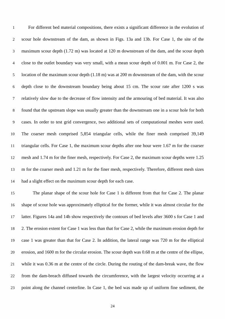
The planar shape of the scour hole for Case 1 is different from that for Case 2. The planar 15

shape of scour hole was approximately elliptical for the former, while it was almost circular for the 16

latter. Figures 14a and 14b show respectively the contours of bed levels after 3600 s for Case 1 and 17

2. The erosion extent for Case 1 was less than that for Case 2, while the maximum erosion depth for 18

case 1 was greater than that for Case 2. In addition, the lateral range was 720 m for the elliptical 19

erosion, and 1600 m for the circular erosion. The scour depth was 0.68 m at the centre of the ellipse, 20

while it was 0.36 m at the centre of the circle. During the routing of the dam-break wave, the flow 21

from the dam-breach diffused towards the circumference, with the largest velocity occurring at a 22

point along the channel centerline. In Case 1, the bed was made up of uniform fine sediment, the 23

25

value of sediment transport capacity was proportional to the velocity. This led to the largest bed 1

scour depth occurring close to the centerline and its value decreased away from the centerline. In 2

Case 2, the bed was composed of graded sediments. All of the sediment fractions close to the 3

channel centerline were scoured due to the relatively large flow velocity, while the flow velocity 4

reduced away from the centerline, the finer sediment fractions were still scoured, which led to a 5

wider planar shape of the scour hole. For Case 2, the composition of bed material had a tendency of 6

armouring due to bed scouring, and the corresponding value of sediment transport capacity 7

decreased gradually. However, for Case 1, the bed material composition did not change during the 8

process of bed evolution, since it had no effect on the value of sediment transport capacity. 9

Therefore, the maximum erosion depth in Case 1 was greater than that in Case 2. 10

6 Concluding remarks 11

In this paper, details are given regarding a 2D morphodynamic model for predicting dam-break 12

flows over mobile beds. The model employs the shallow water equations for turbid waters, which 13

take into account the effects of sediment density and bed level changes on the flood flows. In 14

addition, the model is capable of simulating the transport of graded suspended load and bed load, 15

and the adjustment of bed material composition. A finite volume method is used to solve the 16

governing equations. The model adopts an unstructured triangular mesh and is second-order 17

accurate in both time and space. A coupled approach has been used to solve simultaneously the flow 18

and sediment transport processes induced by dam-breaks, in which flood wave fronts move rapidly 19

and lead to significant bed level changes. 20

The model was verified against the predictions from existing numerical models and laboratory 21

experimental data published in the literature, including two test cases of flow over fixed beds and 22

two cases of flow over mobile beds. It was then used to investigate the influences of different 23

26

bed-material compositions on the hydrodynamics and morphology of a channel. It is demonstrated 1

that the model is capable of simulating the interactive processes between the water flow, sediment 2

transport and morphological changes caused by dam-break flows for different bed material 3

compositions. From the model predictions it has been found that the behaviour of dam-break flows 4

over a mobile bed is significantly different from that over a fixed bed. The main findings from these 5

tests are that: 6

(i) For a dam-break induced flow at the initial stage, the rate of bed evolution is comparable 7

to the rate of water depth variation near the dam site; 8

(ii) For mobile beds, the erosion extent over the uniform sediment bed is less than that over 9

the non-uniform sediment bed, while the maximum erosion depth obtained over the 10

former is greater than that over the latter; and 11

(iii) The planar shape of the scour hole is approximately elliptical over the uniform sediment 12

bed and it is almost circular over the non-uniform sediment bed, which indicates 13

increased erosion in the lateral direction. 14

Acknowledgements 15

The research reported in this paper was conducted as part of the Flood Risk Management 16

Research Consortium (Phase II), supported by the UK Engineering and Physical Sciences Research 17

Council (GR/S76304). The National Basic Research Program of China (2007CB714102) 18

“Mechanisms of dam and levee breaking under complex uncertainties and theories of risk 19

mitigation and control” is also gratefully acknowledged. Another National Basic Research Program 20

of China (2006CB403303) is appreciated for offering the experimental data of the forth test case in 21

the model verification. Lastly, the authors thank very much the reviewers for their constructive 22

27

comments that improved the paper. 1

References 2

[1] Stoker JJ. Water waves. Pure and applied mathematics, Vol. (IV). Interscience Publishers: New 3

York; 1957. 4

[2] Chanson H. Analytical Solution of Dam Break Wave with Flow Resistance: Application to 5

Tsunami Surges. In: Proceedings of the 31st IAHR Biennial Congress, eds. Jun BH, Lee SI, Seo 6

IW and Choi GW. Seoul, Korea 2005; p3341-3353 7

[3] Lin GF, Lai JS and Guo WD. Finite-volume component-wise TVD schemes for 2D shallow 8

water equations. Advances in Water Resources 2003; 26: 861-873. 9

[4] Fagherazzi S and Sun T. Numerical simulations of transportational cyclic steps. Computers and 10

Geosciences 2003; 29: 1143-1154. 11

[5] Liao CB, Wu MS and Liang SJ. Numerical simulation of a dam break for an actual river terrain 12

environment. Hydrological Processes 2007; 21: 447-460. 13

[6] Wu WM and Wang SSY. One-dimensional modeling of dam-break flow over movable beds. 14

ASCE Journal of Hydraulic Engineering 2007; 133(1):48-58. 15

[7] Zech Y, Soares-Frazão S and Spinewine B. Dam-break induced sediment movement: 16

Experimental approaches and numerical modeling. Journal of Hydraulic Research 2008; 46(2): 17

176-190. 18

[8] Zhou JG, Causon DM, Mingham CG. and Ingram DM. Numerical prediction of dam-break 19

flows in general geometries with complex bed topography. ASCE Journal of Hydraulic 20

Engineering 2004; 130(4): 332-340. 21

[9] Liang DF, Lin BL and Falconer RA. A boundary-fitted numerical model for flood routing with 22

shock-capturing capability. Journal of Hydrology 2007; 332: 477-486. 23

[10] Begnudelli L and Sanders BF. Conservative wetting and drying methodology for quadrilateral 24

grid finite-volume models. ASCE Journal of Hydraulic Engineering 2007; 133(3): 312–322. 25

[11] Gallegos HA, Schubert JE and Sanders BF. Two-dimensional, high-resolution modeling of 26

28

urban dam-break flooding: A case study of Baldwin Hills, California. Advance in Water 1

Resources 2009; 32: 1323-1335 2

[12] Costa JE and Schuster RL. The formation and failure of natural dams. Geological Society of 3

America Bulletin 1988; 100(7): 1054-1068. 4

[13] Capart H, Young DL and Zech Y. Dam-break Induced debris flow and particulate gravity 5

currents. Special Publication of the International Association of Sedimentologists (eds. Kneller 6

B, McCaffrey B, Peakall J and Druitt T) 2001; 31: 149-156. 7

[14] Kale VS, Ely LL, Enzel Y and Baker VR. Geomorphic and hydrologic aspects of mon-soon 8

floods on the Narmada andTapi Rivers in central India. Geomorphology 1994; 10:157-168. 9

[15] Zhang RJ and Xie JH. Sedimentation Research in China. China Water and Power Press, Beijing; 10

1993. 11

[16] Ferreira R and Leal J. 1D mathematical modeling of the instantaneous dam-break flood wave 12

over mobile bed: Application of TVD and flux-splitting schemes. Proceedings of the European 13

Concerted Action on Dam-Break Modeling, Munich, 1998; pp 175-222. 14

[17] Fraccarollo L and Armanini A. A semi-analytical solution for the dam-break problem over a 15

movable bed. Proceedings of the European Concerted Action on Dam-Break Modeling, Munich, 16

1998; pp 145-152. 17

[18] Fraccarollo L and Capart H. Riemann wave description of erosional dam-break flows. Journal 18

of Fluid Mechanics 2002; 461: 183-228. 19

[19] Spinewine B and Zech Y. Small-scale laboratory dam-break waves on movable beds. IAHR 20

Journal of Hydraulic Research 2007; 45(Extra Issue): 73-86 21

[20] Cao Z, Pender G, Wallis S and Carling P. Computational dam-break hydraulics over mobile 22

sediment bed. ASCE Journal of Hydraulic Engineering 2004; 130(7): 689-703. 23

[21] Cao Z, Li Y and Yue Z. Multiple time scales of alluvial rivers carrying suspended sediment and 24

their implications for mathematical modeling. Advance in Water Resources 2007; 30(4): 25

715-729. 26

29

[22] Hu P and Cao Z. Fully coupled mathematical modeling of turbidity currents over erodible bed. 1

Advance in Water Resources 2009; 32(1):1-15. 2

[23] Fraccarollo L and Toro EF. Experimental and numerical assessment of the shallow water model 3

for two-dimensional dam-break type problems. IAHR Journal of Hydraulic Research 1995; 4

33(6): 843-864. 5

[24] Zhao DH, Shen HW, Lai JS and Tabios III GQ. Approximate Riemann solvers in FVM for 2D 6

hydraulic shock wave modelling. ASCE Journal of Hydraulical Engineering 1996; 122 (12): 7

692-702. 8

[25] Simpson G and Castelltort S. Coupled model of surface water flow, sediment transport and 9

morphological evolution. Computers and Geosciences, 2006; 32: 1600-1614. 10

[26] Cao Z. Comments on the paper by Guy Simpson and Sebastien Castelltort “Coupled model of 11

surface water flow, sediment transport and morphological evolution”. Computers and 12

Geosciences 2007; 33: 976-978. 13

[27] Xie JH. River modelling. Beijing: China Water and Power Press 1990; (in Chinese). 14

[28] Yue ZY, Cao ZX, Li X and Che T. Two-dimensional coupled mathematical modeling of fluvial 15

processes with intense sediment transport and rapid bed evolution. Science in China (Series G) 16

2008; 51(9): 1427-1438 17

[29] Zhou JJ and Lin BN. One-dimensional mathematical model for suspended sediment by lateral 18

integration. ASCE Journal of Hydraulic Engineering 1998; 124(7): 712-717. 19

[30] Wang GQ and Xia JQ. Channel widening during the degradation of alluvial rivers, International 20

Journal of Sediment Research 2001; 16(2): 139-149. 21

[31] Dou XP, Li TL and Dou GR. Numerical model of total sediment transport in the Yangtze 22

Estuary. China Ocean Engineering 1999; 13(3): 277-286. 23

[32] Wu WM. Depth-averaged 2D numerical modeling of unsteady flow and nonuniform sediment 24

transport in open channels. ASCE Journal of Hydraulic Engineering 2004; 130(10): 1013-1024. 25

[33] Wu BS and Long YQ. Corrections for the formula of sediment transport capacity in the Yellow 26

30

River. Yellow River 1993; (7): 1-4 (in Chinese). 1

[34] Wang GQ, Xia JQ and Wu BS. Numerical simulation of longitudinal and lateral channel 2

deformations in the braided reach. ASCE Journal of Hydraulic Engineering 2008; 134(8): 3

1064-1078. 4

[35] Caleffi V, Valiani A and Zanni A. Finite volume method for simulating extreme flood events in 5

natural channels. IAHR Journal of Hydraulic Research 2003; 41(2): 167-177. 6

[36] Wang JW and Liu RX. A comparative study of finite volume methods on unstructured meshes 7

for simulation of 2D shallow water wave problems. Mathematics and Computers in Simulation 8

2004; 53: 171-184. 9

[37] Yoon TH and Kang SK. Finite volume model for two-dimensional shallow water flows on 10

unstructured grids. ASCE Journal of Hydraulic Engineering 2004; 130(7): 678-688. 11

[38] Xia JQ, Falconer RA, Lin BL and Wang GQ. Modelling floods routing on initially dry beds by 12

a TVD finite volume method. International Journal for Numerical methods in Fluids 2009; (in 13

press). 14

[39] Liang L, Ni JR, Borthwick AGL and Rogers BD. Simulation of dike-break processes in the 15

Yellow River. Science in China (Ser. E) 2002; 45(6): 606-619. 16

[40] Godunov SK. A difference method for the numerical calculation of discontinuous solutions of 17

hydrodynamic equations. Matemsticheskly Sboraik 47. (US Joint Publications Research 18

Service); 1959. 19

[41] Fraccarollo L and Toro EF. Experimental and numerical assessment of the shallow water model 20

for two-dimensional dam-break type problems. IAHR Journal of Hydraulic Research 1995; 21

33(6): 843-864. 22

[42] Toro EF. Shock-capturing methods for free-surface shallow flows. John Wiley and Sons, 2001, 23

326p. 24

[43] Sleigh PA, Gaskell PH, Berzins M and Wright NG. An unstructured finite-volume algorithm for 25

predicting flow in rivers and estuaries. Computers and Fluids 1998; 27(4): 479-508. 26

31

[44] Roe PL. Approximate Riemann solvers, parameter vectors and difference schemes. Journal of 1

Computational Physics 1981; 43: 357-372. 2

[45] Van Leer B. Towards the ultimate conservative difference scheme. V. A. second order sequel to 3

Godunov’s method. Journal of Computational Physics 1979; 32: 101-136. 4

[46] Roe PL and Baines MJ. Algorithms for advection and shock problems. In: Viviand H, editor. 5

Proceedings of the Fourth GAMM Conference on Numerical Methods in Fluid Mechanics. 6

Braunschweig: Vieweg, 1981; 281-290. 7

[47] Tan WY. Shallow water hydrodynamics. New York: Elsevier; 1992. 8

[48] Zhao DH, Shen HW, Tabios III GQ, Lai JS and Tan WY. Finite-volume two-dimensional 9

unsteady flow model for river basins. ASCE Journal of Hydraulic Engineering 1994; 120(7), 10

863-883. 11

[49] Brufau P, Garcia-Navarro P and Vazquez-Cendon ME. Zero mass error using unsteady 12

wetting-drying conditions in shallow flows over dry irregular topography. International Journal 13

for Numerical Methods in Fluids 2004; 45: 1047-1082. 14

[50] Bradford SF and Sanders BF. Finite-volume model for shallow water flooding of arbitrary 15

topography. ASCE Journal of Hydraulic Engineering 2002; 128(3): 289-298. 16

[51] Falconer RA and Chen Y. An improved representation of flooding and drying and wind stress 17

effects in a 2D tidal numerical model. Proceedings of the Institution of Civil Engineers 1991; 18

2(2): 659-672. 19

[52] Fennema RJ and Chaudhry MH. Explicit methods for 2D transient free-surface flows. ASCE 20

Journal of Hydraulic Engineering 1990; 116(8): 1013-1034. 21

[53] Bellos V, Soulis JV and Sakkas JG. Experimental investigations of two dimensional 22

dam-break-induced flows. IAHR Journal of Hydraulic Research 1992; 30(1): 47-63. 23

[54] Palumbo A, Soares-Frazão S, Goutiere L, Pianese D and Zech Y. Dam-break flow on mobile 24

bed in a channel with a sudden enlargement. In: Proceedings of River Flow 2008. Aydin, 25

Cokgor and Kirkgoz (eds), Turkey, 2008; pp. 645-654. 26

32

1

y

x

i

nx

ny

lij

Ai

a

b

n

m

Ui

Uj

Um

UL

UR

o

Aj

Ukk

j=3

j=2

j=1

cell node

cell centre

SL

SR

2

Fig. 1 Sketch of a control volume 3

4

5

6

X(m)

0

40

80

120

160

200

Y(m)

0

40

80

120

160

200

Z(m

)

5

6

7

8

9

10

X(m)

Y(m

)

0 40 80 120 160 2000

40

80

120

160

2005.5 6 6.5 7 7.5 8 8.5 9

2 m/s

Water level(m)

7

8

Fig. 2 Simulated results at t = 7.2 s: (a) water level and (b) velocity field 9

10

(a) (b)

33

1

2

3

-0.2

0.0

0.2

0.4

0.6

0.8

1.0

1.2

1.4

1.6

-10 -8 -6 -4 -2 0 2 4 6 8 10 12 14X(m)

Y(m

)

Observation Points

P1 P2

P3

P4

P1 (x=-8.50 m)P2 (x=-4.00 m)P3 (x=+2.50 m)P4 (x=+10.0 m)

Wall

Ope

n

Dam

4

Fig. 3 Sketch of a dam-break flow experiment in a converging-diverging channel 5

6

7

(a)Location: P1

0.00

0.05

0.10

0.15

0.20

0.25

0.30

0 10 20 30 40 50 60Time(s)

Wa

ter

de

pth

(m

) Obs.

Cal.

(b)Location: P2

0.00

0.05

0.10

0.15

0.20

0.25

0.30

0 10 20 30 40 50 60Time(s)

Wa

ter

de

pth

(m

) Obs.

Cal.

(c)Location: P3

0.00

0.04

0.08

0.12

0.16

0.20

0 10 20 30 40 50 60Time(s)

Wa

ter

de

pth

(m

) Obs.

Cal.

(d) Location: P4

0.00

0.04

0.08

0.12

0.16

0.20

0 10 20 30 40 50 60Time(s)

Wa

ter

leve

l (m

) Obs.

Cal.

8

Fig. 4 Comparisons between the observed and calculated water depths 9

10

11

12

13

Fre

e ou

tflo

w B

D

34

1

0.0

0.1

0.2

0.3

0.4

0.5

0.6

0.0 1.0 2.0 3.0 4.0 5.0 6.0

X(m)

Y(m

)

Observation Points 1-6

Observation CS 1-2

Dam F

ree

ou

tflo

w B

D

1 2 3 4

65

CS

1

CS

2

Initial depth = 25cm

2

Fig. 5 Sketch of a dam-break flow experiment over a mobile bed 3

4

0.08

0.10

0.12

0.14

0.16

0.18

0.20

0.22

0 2 4 6 8 10 12

Time(s)

Z (

m) Exp.at P1

Cal.at P1

0.08

0.10

0.12

0.14

0.16

0.18

0.20

0.22

0 2 4 6 8 10 12

Time(s)

Z (

m) Exp.at P5

Cal.at P5

0.08

0.10

0.12

0.14

0.16

0.18

0.20

0.22

0 2 4 6 8 10 12

Time(s)

Z (

m) Exp.at P2

Cal.at P2

0.08

0.10

0.12

0.14

0.16

0.18

0.20

0.22

0 2 4 6 8 10 12

Time(s)

Z (

m) Exp.at P3

Cal.at P3

0.08

0.10

0.12

0.14

0.16

0.18

0.20

0.22

0 2 4 6 8 10 12

Time(s)

Z (

m) Exp.at P6

Cal.at P6

0.08

0.10

0.12

0.14

0.16

0.18

0.20

0.22

0 2 4 6 8 10 12

Time(s)

Z (

m) Exp.at P4

Cal.at P4

5

Fig. 6 Comparisons between the observed and calculated water levels 6

35

(a) CS1 at X=4.1m

0.07

0.08

0.09

0.10

0.11

0.12

0.13

0.14

0.15

0 0.1 0.2 0.3 0.4 0.5

Y(m)Z

b(m

) Initial

Exp.

Cal.

(b) CS2 at X=4.4m

0.07

0.08

0.09

0.10

0.11

0.12

0.13

0.14

0.15

0 0.1 0.2 0.3 0.4 0.5

Y(m)

Zb

(m) Initial

Exp.Cal.

1

Fig. 7 Comparisons between the observed and calculated cross-sectional profiles 2

3

-0.2

0.0

0.2

0.4

0.6

0.8

1.0

1.2

1.4

1.6

1.8

-2 0 2 4 6 8 10 12 14 16 18 20x(m)

y(m

)

Co

al a

sh

Non-erodible bed

Wat

er

Fre

e o

utf

low

BD

2m 4.5m 12m

CS1 CS2

4

Fig. 8 Sketch of a dam-breach flow experiment over a mobile bed 5

6

36

-0.16

-0.13

-0.10

-0.07

-0.04

-0.01

0.02

0 0.2 0.4 0.6 0.8 1 1.2 1.4 1.6

Y(m)Z

b(m

)

Ini.Exp.Cal.

z

(a)CS1( x=2.5m)

-0.16

-0.13

-0.10

-0.07

-0.04

-0.01

0.02

0 0.2 0.4 0.6 0.8 1 1.2 1.4 1.6

Y(m)

Zb

(m)

Ini.

Exp.

Cal.

(b)CS2( x=3.5m)

1

Fig. 9 Comparisons between the observed and calculated cross-sectional profiles 2

3

-200

0

200

400

600

800

1000

1200

1400

1600

1800

2000

2200

-200 0 200 400 600 800 1000 1200 1400 1600 1800 2000 2200

x(m)

y(m

)

200m

P1 P2

initi

al d

ept

h =

5m

dry

be

d

fre

e o

utflo

w B

D

4

Fig. 10 Sketch of a partial dam-breach flow 5

37

1

-1.6

-1.2

-0.8

-0.4

0.0

0.4

0.8

1.2

1.6

2.0

0 600 1200 1800 2400 3000 3600Time (s)

Wa

ter

/ Be

d le

vel (

m)

Case 0

Case 1

Case 2

Case 0

Case 1

Case 2

( a)

-0.5

-0.1

0.3

0.7

1.1

1.5

0 600 1200 1800 2400 3000 3600Time (s)

Wa

ter

/ Be

d le

vel (

m)

Case 0

Case 1

Case 2

Case 0

Case 1

Case 2

( b)

Wat

er

Wa

ter

Be

d Be

d

2

Fig. 11 Water level and bed level variations downstream of the dam for (a) P1 and (b) P2 3

4

0

20

40

60

80

100

600 800 1000 1200 1400 1600 1800 2000Distance along the channel (m)

Co

nce

ntra

tion

(kg/

m3)

t=0st=600st=1200st=1800st=2400st=3000st=3600s

( a)

0

20

40

60

80

100

600 800 1000 1200 1400 1600 1800 2000Distance along the channel (m)

Con

cen

trat

ion

(kg

/m3) t=0s

t=600st=1200st=1800st=2400st=3000st=3600s

( b)

5

Fig. 12 Variations of sediment concentrations along the channel centerline for (a) Case 1 and (b) Case 2 6

7

-1.8

-1.6

-1.4

-1.2

-1.0

-0.8

-0.6

-0.4

-0.2

0.0

0.2

600 800 1000 1200 1400 1600 1800 2000Distance along the channel (m)

Be

d L

eve

l (m

)

t=0st=600st=1200st=1800st=2400st=3000st=3600s

( a)

-1.8

-1.6

-1.4

-1.2

-1.0

-0.8

-0.6

-0.4

-0.2

0.0

0.2

600 800 1000 1200 1400 1600 1800 2000Distance along the channel (m)

Bed

Le

vel (

m)

t=0st=600st=1200st=1800st=2400st=3000st=3600s

( b)

8

Fig. 13 Variations of longitudinal bed profiles along the channel centerline for (a) Case 1 and (b) Case 2 9

10

11

38

-1.4

-1.4

-1.2

-1

-1

-0.8

-0.6

-0.4

-0.4

-0.2

-0.2

-0.2

-0.1

-0.1

-0.1

X(m)

Y(m

)

800 900 1000 1100 1200 1300 1400 1500 1600 1700 1800 1900 2000200

300

400

500

600

700

800

900

1000

1100

1200

1300

1400

1500

1600

1700

1800

-0.1-0.2-0.4-0.6-0.8-1-1.2-1.4-1.6

Scour depth(m) (a)

-1

-0.8

-0.6

-0.6-0.4

-0.2

-0.2

-0.2

-0.2

-0.1

-0.1

-0.1

X(m)Y

(m)

800 900 1000 1100 1200 1300 1400 1500 1600 1700 1800 1900 2000200

300

400

500

600

700

800

900

1000

1100

1200

1300

1400

1500

1600

1700

1800

-0.1-0.2-0.4-0.6-0.8-1-1.2-1.4-1.6

Scour depth(m) (b)

1

Fig. 14 Contours of bed levels after 3600s for (a) Case 1 and (b) Case 2 2

3

4

5

6

7

8

9

10

11

12

13

14

15

16

39

Table 1 Parameters used in test and application cases 1

2

No Parameters

Values used

Test case 1

Test case2

Test case 3

Test case 4

Application case

1 in t turbulent viscosity coefficient 0.5 0.5 0.5 0.5 0.5 2 n (Manning n ) 0.00 0.012 0.025 0.015 0.015

3 in sk (non-equilibrium adaptation

coefficient of suspended load) 0.50 0.50

4 bk = (non-equilibrium adaptation

coefficient of bed load) 0.90

5 in kP* ( percentage of sediment

transport capacity) 0.90 0.90

6 bK in Eq.(7) (transport capacity of bed

load) 0.10

3

4

Table 2 Error analysis results 5

6

Tests Sources Descriptions of error analysis for each test case

Test1 Fennema and Chaudhry [52]

No analytical solution, the predicted water level and velocity distributions agree closely with those obtained from the existing models.

Test2 Bellos et al. [53]

The correlation coefficients reach 0.998 at the two upstream measurement points. The predicted mean depths at the two downstream measurement points are about 10% higher than the measurements.

Test3 Palumbo et al. [54]

The correlation coefficient between the predicted and observed water level hydrographs ranges from 0.6 to 0.9. The predicted mean bed level is 3.7% lower than the observed one at CS1, and is 5.8% lower than the observed one at CS2.

Test4 Tsinghua experiment

The predicted mean bed level is about 1.7 cm or 35% higher than the observed one at CS1, and is about 0.6 cm or 60% lower than the observed one at CS2.

7

8