Western Australia School of Mines: Minerals, Energy and Chemical

Engineering

Modelling and simulation of biomass fast pyrolysis process:

Kinetics, reactor, and condenser systems

Adhirath Sanjay Wagh

This thesis is presented for the Degree of

Doctor of Philosophy

Of

Curtin University

February 2019

Declaration

To the best of my knowledge and belief, this thesis contains no material previ-

ously published by any other person except where due acknowledgement has

been made.

This thesis contains no material which has been accepted for the award of any

other degree or diploma in any university.

Date: 22/02/2019

i

To,

My Parents,

Family & Friends,

and Teachers

ii

Acknowledgement

"Thank you" is not sufficient to express how I feel about everyone’s contribution

not only to this work but also towards my development.

I would first like to thank my supervisors, Head of School, Prof. Vishnu Pareek,

Dr. Ranjeet Utikar, and Prof. J. B. Joshi for giving me this oppportunity to work

at Curtin University. I would also like to thank Curtin Univeristy (CIPRS) to grant

me a scholarship for my Ph.D. tenure.

Prof. Vishnu Pareek has been a constant source of inspiration and alwaysmotivat-

ing me throughout this journey. Apart from his help with the research his ability

of working with people has helped me overcome few of my own barriers. He has

been very patient with me, and I want to thank him for this specially.

I would like to express my deep gratitude towards Prof. J.B. Joshi, whose life long

teaching spirit, curiosity, intellect, and humble character are a source of inspira-

tion for me. His guidance has been very crucial for deciding my thesis structure.

Dr. Ranjeet Utikar has been a constant inspiration for me. I would especially like

to thank him formotivating, in his ownway, me to do bettermy best. I learned the

most from his approach of defining a problem and finding its solution. He always

motivates everyone to read and explore about innovations in different areas of

science and engineering. This led me to watch documentaries about innovations

and read about the work of eminent scientists. He does like things to be perfect

and his persuasion helped improve my presentation skills. I got to learn about a

lot of software tools which have andwill helpme. Thanks to him for changing and

helping me develop a new approach of solving problems.

Thank you very much Manju ma’am for being very kind and empathetic towards

all of us. Awesome food, kind words, and happy moments with you are the mo-

ments Iwill cherish for the rest ofmy life. And aswediscussed, thankyouwouldn’t

iii

put a full stop, I will definitely be in touch with a person like you.

A special thank you to Dr. Yogesh Shinde and Dr. Abhishek Sharma for their help

with experiments and analysis of the work. Their inputs have been very valuable.

Thanks a ton to Dr. Sharmilee Mane. She is the reason I am here. I met her back

in ICT and she suggested me to apply in Curtin University. Coming to Curtin has

helped me improve by leaps and bounds; so a special thank you to Sharmilee.

Mrunmai, Sanket (Shankar), and Subhra, you guysmademy journey very smooth.

Special thanks to Mrunmai for bearing me and for being always there to help.

Your kind words and unconditional support made me stand up to all the prob-

lems. The meals at different restaurants were really soothing. Mrunmai I really

have no words for your support, it has been of utmost importance. Your sugges-

tion of pursuing a Ph.D. was the best decision I took. Thanks a lot. I got to meet

two really awesome guys, Sanket and Subhra. Thanks a lot sanket for helping me

out when I came here. You made it very easy. Conversations about your school

and our discussions to work in the area of education were really enlightening. I

would really like to work with you on this in the future. I really hope I become as

organized as you someday; and witty too. I had cool conversations with Subhra,

and thanks to him that I got into photography. I really see a close friend in you

Sanket and Subhra.

Thanks to the Wongies...Cathy, David, little Joshua, and cute Jesslyn. It was excel-

lent and best experience living with them. Somuch fun and happymoments with

all of you.

Thanks to Barani, Shambhu, Vaibhav, Himanshu, Vishal, Hari, Asha, Pankaj, Jay,

Sakshi, Nimrat, Anupam, Ruturaj, and Rofia for the happy moments in Perth.

Thanks a lot to Jason, Araya, Roshanak, Ann, Andrew, Jimmy, and Melisa for con-

stant support in the lab. Your assistance was really invaluable.

Thanks to my parents, family, and friends in India without whom I wouldn’t have

been here. Thanks to Perth, these years have been the golden years of my life.

iv

Abstract

Biomass pyrolysis has not gained a lot of commercial success because of complex

feedstock chemistry, bio-oil instability, poor fuel properties, and variation in oil

composition with respect to feedstock chemistry and reaction conditions. Com-

putational models can help understand various multiscale processes of biomass

pyrolysis and help in efficient design and sustainable operation of large scale py-

rolysis plants. Reactor and downstream unit operation modeling is challenging

because of chemical composition of pyrolysis products which is significantly af-

fected by complex interplay between reaction kinetics and intra-particle physical,

morphological changes, and transport processes. In this thesis detailed reaction

kinetics, a reaction engineeringmodel of bubblingfluidized bed reactor, and simu-

lation methodology and schemes were developed to address different multi-scale

challenges associated with biomass pyrolysis.

TGA experiments were carried out to study the effect of heating rate and particle

size on biomass pyrolysis rate. A multi-component distributed activation energy

model was used to describe pyrolysis kinetics. The model parameters varied de-

pendingon the biomass particle size aswell as on the choice of data-set obtained at

different heating rates used to calculate the parameters. This could be attributed

to morphological changes in biomass particles beyond a particular heating rate,

which indicated dominance of devolatilization reactions over cross-linking reac-

tions. The study systematically showcased the importance of appropriate choice

of experimental data-set to accurately model fast pyrolysis kinetics. A detailed

reaction model, reported in the literature, was modified by coupling it with the

distributed activation energy model to extend the model’s applicability to wide

range of heating rates and account for effects of morphological changes on reac-

tion rate.

v

To compare the prediction ability of modified kinetics with literature model, an

extensible reaction engineering model of bubbling bed reactor (BBR) was devel-

oped based on the mixing cell approach. The BBR model was used to simulate

biomass pyrolysis process using thedetailed lumpedkineticmodel (solid devolatiliza-

tion reactions) and a rigorous secondary reactionmechanism (Gas phase reactions

with 511 species and 20,239 reactions). The reactor model coupled with reaction

kineticswas validated using literature data. The reactormodel predicted the com-

position of major components of bio-oil and pyrolysis gases.

Finally, simulations for fractional condensation of a mixture of model compounds

(similar to those used in reaction kinetics) representing pyrolysis vapor were car-

ried out. The objective of the study was to fractionally condense the model com-

pounds in distinct chemical families to address the stability issue of bio-oil. A

simulation strategy was developed to design liquid collection systems for biomass

pyrolysis process. Based on the analysis a new multi-stage condensation scheme

was proposed to collect bio-oil in individual chemical families.

The detailed reaction kinetics coupled with DAE approach extends the applicabil-

ity of kinetic model to a wide range of heating rates and also quantifies the effect

of morphological changes on reaction rate. The reactor model proposed in the

present work can be used to simulate biomass pyrolysis process at plant scale.

The pyrolysis reactor model predicts composition of major liquid and gas species

for a wide range of feedstock chemistry and operating conditions (temperature

and heating rate) at plant scale. The bio-oil composition can be further utilized to

design robust downstream processes to achieve a constant throughput of chemi-

cals and fuels for different lignocellulosic biomass. The modeling and simulation

strategies developed in the present research address the scale-up challenges as-

sociated with variable feedstock chemistry, multiphase nature of pyrolysis reac-

tions, and bio-oil instability.

Keywords: biomass, fast pyrolysis, modeling, simulation, reaction kinetics, flu-

idized bed, reactor engineering, bio-oil, multi-stage condensation, fractionation

vi

Nomenclature

General symbols

a, A cross sectional area, m2

A0 frequency factor, 1/s

Ar Archimedes number

As surface area, m2

Bi Biot number

Cp Specific heat capacity, J/kg/K

d diameter, m

D diffusivity, m2/s

E activation energy, kJ/mol

E0 mean activation energy, kJ/mol

fc ratio of cloud phase to bubble phase volume fraction

fw ratio of wake phase to bubble phase volume fraction

g gravitational constant, m/s2

h heat transfer coefficient, W/m2/K

hce, hbc heat transfer rate constant between cloud emulsion andbubble cloud

phase, 1/s

H height of bed in reactor, m

vii

J1, J2, J3 normalized error

kce, kbc mass transfer rate constant between cloud emulsion andbubble cloud

phase, m3/s

kpy pyrolysis reaction rate, 1/s

L characteristic length, m

m mass flow rate, kg/s

m temperature exponent for frequency factor

n mole fraction or splitting parameter to determine biomass composi-

tion

P pressure, N/m2

Py Pyrolysis number

r radius, m

Rep particle Reynold’s number

T temperature, K

t time, s

u velocity, m/s

V volume, m3

wc pseudo component mass fraction

x,X,Y mass fraction

y peak maximum for first derivative of TGA data

z peak maximum for second derivative of TGA data

viii

Greek symbols

α conversion

β heating rate, K/s

γ solid distribution coefficient

δ bubble volume fraction

ε hold up

λ thermal conductivity, W/m/K

ρ density, kg/m3

σ standard deviation in probability distribution function, kJ/mol

Abbreviations

A2 Avrami-Erofeev nucleation model

ACAC acetic acid

BFB bubbling fluidized bed

Cell cellulose

CellA active cellulose

CF chemical family

CFB circulating fluidized bed

CPD chemical percolation devolatilization

DAEM distributed activation energy model

DAXP dianhydro xylo-pyranose

DP depolymeriation reaction model

ix

DTG differential thermal gravimetric data/ curve

ESP electro-static precipitator

F1 first order reaction model

FE2MACR sinapylaldehyde

FG-DVC functional group, depolymerization, vaporization and cross-linking

GMSW glucomannan soft wood

HCE1 active hemicellulose

HCE2 active hemicellulose

HMWL high molecular weight lignin

ITANN 3,5-dihydro benzofuran

LCB lignocellulosic biomass

LIG intermediate solid lignin component

LIGCC intermediate solid lignin component

LIGOH intermediate solid lignin component

LIGC lignin sub-component rich in carbon

LIGH lignin sub-component rich in hydrogen

LIGO lignin sub-component rich in oxygen

LMWC low molecular weight components

MW molecular weight

NBE number of bubble to emulsion mixing cells

NCG non-condensible gas

NRTL non-random two-liquid model

NTH Nothnagel

x

RCR rotating cone reactor

SF separation factor

STHE shell and tube heat exchanger

TANN tannins

TGA thermal gravimetric analysis

TGL triglycerides

UNIFAC UNIQUAC functional-group activity coefficient model

UNIQUAC universal quasichemical activity coefficient model

XYHW xylan hardwood

Subscripts

b bubble phase

B biomass

bed reactor dense bed

c cloud phase

C char

cw cloud-wake phase

e emulsion phase

fb free-board region

g gas phase

i,j component or reaction number

M moisture

mf minimum fluidization

xi

mix mixture

p pseudo-component

pe effective particle properties

py pyrolysis

rj jth reaction

s solid

s,d solid downward direction

SV surface area to volume ratio of spherical particle with effective di-

ameter

V volume of spherical particle with effective diameter

α splitting parameter between cellulose and hemicellulose

β splitting parameter between lignin sub-component LIG-H and LIG-C

γ splitting parameter between lignin sub-component LIG-O and LIG-C

δ splitting parameter between lignin and triglyceride

ε splitting parameter between lignin and tannin

Superscripts

ith emulsion, bubble, cloud phase mixing cell number

pri primary reactions

q shape factor

sec secondary reactions

∗ maximum volatiles

xii

Contents

1 Introduction 2

1.1 Introduction . . . . . . . . . . . . . . . . . . . . . . . . . . . . . . 2

1.2 Background . . . . . . . . . . . . . . . . . . . . . . . . . . . . . . . 2

1.3 Motivation . . . . . . . . . . . . . . . . . . . . . . . . . . . . . . . 5

1.3.1 Challenges . . . . . . . . . . . . . . . . . . . . . . . . . . . 5

1.3.2 Research significance . . . . . . . . . . . . . . . . . . . . . 7

1.4 Research Objectives . . . . . . . . . . . . . . . . . . . . . . . . . . . 8

1.5 Thesis Outline . . . . . . . . . . . . . . . . . . . . . . . . . . . . . . 8

2 Literature review 10

2.1 Introduction . . . . . . . . . . . . . . . . . . . . . . . . . . . . . . 10

2.2 LCB as a renewable carbon resource . . . . . . . . . . . . . . . . . . 11

2.2.1 Chemical structure . . . . . . . . . . . . . . . . . . . . . . . 11

2.2.2 Physical structure . . . . . . . . . . . . . . . . . . . . . . . 12

2.2.3 Biomass conversion technologies . . . . . . . . . . . . . . . 13

2.3 Fast pyrolysis of LCB . . . . . . . . . . . . . . . . . . . . . . . . . . 15

2.3.1 Multiphase and multiscale pyrolysis chemistry . . . . . . . 15

2.3.2 Biomass pyrolysis kinetic modeling . . . . . . . . . . . . . . 17

2.4 Fast pyrolysis reactors . . . . . . . . . . . . . . . . . . . . . . . . . 28

2.4.1 Rotating cone reactor . . . . . . . . . . . . . . . . . . . . . 30

2.4.2 Ablative reactor . . . . . . . . . . . . . . . . . . . . . . . . 32

2.4.3 Auger reactor . . . . . . . . . . . . . . . . . . . . . . . . . . 32

2.4.4 Circulating fluidized bed reactor . . . . . . . . . . . . . . . 33

2.4.5 Bubbling fluidized bed reactor . . . . . . . . . . . . . . . . . 33

2.5 Fast pyrolysis bio-oil . . . . . . . . . . . . . . . . . . . . . . . . . . 35

xiii

2.5.1 Physical and chemical properties of bio-oil . . . . . . . . . . 35

2.5.2 Catalytic upgradation of bio-oil . . . . . . . . . . . . . . . . 44

2.5.3 Fractional condensation of pyrolysis vapors . . . . . . . . . 44

2.6 Significance of this research . . . . . . . . . . . . . . . . . . . . . . 51

3 Modeling pyrolysis kinetics using DAEM 54

3.1 Introduction . . . . . . . . . . . . . . . . . . . . . . . . . . . . . . 54

3.2 Significance of experimental methodology . . . . . . . . . . . . . . 56

3.3 Isoconversion Methods for Kinetic analysis . . . . . . . . . . . . . . 58

3.4 Distributed Activation Energy Model . . . . . . . . . . . . . . . . . 59

3.4.1 Assumptions . . . . . . . . . . . . . . . . . . . . . . . . . . 60

3.4.2 Mathematical model . . . . . . . . . . . . . . . . . . . . . . 60

3.4.3 DAEM equations used for parameter optimization . . . . . . 65

3.5 Materials and methods . . . . . . . . . . . . . . . . . . . . . . . . . 67

3.5.1 Biomass Analysis . . . . . . . . . . . . . . . . . . . . . . . . 67

3.5.2 TGA Calibration . . . . . . . . . . . . . . . . . . . . . . . . . 67

3.5.3 Thermogravimetric analysis of biomass . . . . . . . . . . . 68

3.5.4 Calculation of DTG curve . . . . . . . . . . . . . . . . . . . . 70

3.5.5 Optimization of DAEM parameters . . . . . . . . . . . . . . 70

3.6 Results and Discussion . . . . . . . . . . . . . . . . . . . . . . . . . 70

3.6.1 Biomass Analysis . . . . . . . . . . . . . . . . . . . . . . . . 70

3.6.2 Thermogravimetric analysis of biomass . . . . . . . . . . . 73

3.6.3 TGA data analysis using isoconversion method . . . . . . . 87

3.6.4 DAEM kinetic parameters . . . . . . . . . . . . . . . . . . . 91

3.7 Summary . . . . . . . . . . . . . . . . . . . . . . . . . . . . . . . . 129

4 DAEM coupled detailed pyrolysis kinetics 130

4.1 Introduction . . . . . . . . . . . . . . . . . . . . . . . . . . . . . . 130

4.2 Mathematical model . . . . . . . . . . . . . . . . . . . . . . . . . . 131

4.2.1 Detailed lumped kinetic model: Ranzi model . . . . . . . . . 131

4.2.2 DAEM coupled modified Ranzi model . . . . . . . . . . . . . 147

4.3 Optimization of DAEM parameters and correction factor . . . . . . 157

4.4 Results and discussion . . . . . . . . . . . . . . . . . . . . . . . . . 159

xiv

4.4.1 Model comparison: Total volatile evolution profile . . . . . 159

4.4.2 Model comparison: Global oil, gas, and char yield . . . . . . 166

4.4.3 Model comparison: Gas and liquid product profile . . . . . . 173

4.5 Summary . . . . . . . . . . . . . . . . . . . . . . . . . . . . . . . . 181

5 Biomass fast pyrolysis: Bubbling fluidized bed reactor modeling 182

5.1 Introduction . . . . . . . . . . . . . . . . . . . . . . . . . . . . . . 182

5.2 Mathematical model . . . . . . . . . . . . . . . . . . . . . . . . . . 183

5.3 Pyrolysis kinetics . . . . . . . . . . . . . . . . . . . . . . . . . . . . 183

5.4 Fluidized bed reaction engineering model . . . . . . . . . . . . . . 184

5.4.1 Emulsion phase balance . . . . . . . . . . . . . . . . . . . . 186

5.4.2 Cloud phase balance . . . . . . . . . . . . . . . . . . . . . . 190

5.4.3 Bubble phase balance . . . . . . . . . . . . . . . . . . . . . 192

5.4.4 Free board region balance . . . . . . . . . . . . . . . . . . . 193

5.4.5 Estimation of hydrodynamic parameters . . . . . . . . . . . 194

5.5 1-D single particle heat conduction . . . . . . . . . . . . . . . . . . 196

5.6 Solution methodology . . . . . . . . . . . . . . . . . . . . . . . . . 197

5.7 Results and discussion . . . . . . . . . . . . . . . . . . . . . . . . . 199

5.7.1 Model Validation . . . . . . . . . . . . . . . . . . . . . . . . 200

5.7.2 Heating rate estimation for biomass particle . . . . . . . . . 200

5.7.3 Estimation of pyrolysis product yields . . . . . . . . . . . . 201

5.8 Summary . . . . . . . . . . . . . . . . . . . . . . . . . . . . . . . . 214

6 Fractional condensation of biomass pyrolysis vapors 215

6.1 Introduction . . . . . . . . . . . . . . . . . . . . . . . . . . . . . . 215

6.2 Modeling fractional condensation . . . . . . . . . . . . . . . . . . . 217

6.2.1 Multistage condensation . . . . . . . . . . . . . . . . . . . . 217

6.2.2 Pyrolysis vapor fractionation . . . . . . . . . . . . . . . . . 219

6.3 Results and discussion . . . . . . . . . . . . . . . . . . . . . . . . . 222

6.3.1 AspenPlus simulation validation . . . . . . . . . . . . . . . 222

6.3.2 Pyrolysis vapor fractionation . . . . . . . . . . . . . . . . . 231

6.4 Summary . . . . . . . . . . . . . . . . . . . . . . . . . . . . . . . . 250

xv

7 Closure and future work 251

7.1 Closure . . . . . . . . . . . . . . . . . . . . . . . . . . . . . . . . . 251

7.2 Future work . . . . . . . . . . . . . . . . . . . . . . . . . . . . . . . 256

A.1 Appendix: Chapter 3 . . . . . . . . . . . . . . . . . . . . . . . . . . 258

A.1.1 Experimental data . . . . . . . . . . . . . . . . . . . . . . . 258

B.1 Appendix: Chapter 6 . . . . . . . . . . . . . . . . . . . . . . . . . . 283

xvi

List of Figures

1.1 Fast pyrolysis: A multiscale problem . . . . . . . . . . . . . . . . . 3

1.2 Interdependence of upstream and downstream pyrolysis process

variables. The shaded area is not addressed in this work. . . . . . . 6

2.1 Representative chemical structure of cellulose, hemicellulose and

lignin . . . . . . . . . . . . . . . . . . . . . . . . . . . . . . . . . . 12

2.2 LCB conversion techniques . . . . . . . . . . . . . . . . . . . . . . . 14

2.3 Multicomponent and multiphase nature of pyrolysis reactions. . . 16

2.4 Morphological changes occurring during biomass pyrolysis. . . . . 17

2.5 Single andmulticomponentmulti-reaction kineticmodels for biomass

pyrolysis. (a) [1, 2]; (b) [3]; (c) [4]; (d) [5]; (e) [6]; (f) [7]; (g) [8]; (h)

[9]; (i),(j),(k) [10]; (l) [11]; (m) [12]. LVG: Levoglucosan; HAA: Hy-

droxyacetaldehyde; HCHO: Formaldehyde; LMWC: Low molecular

weight compounds; Int: Intermediate; TG: trapped gases in meta-

plast γ: Stoichiometric coefficient; i: component id . . . . . . . . . 18

2.6 Reaction-transport process regimemap calculated with h = 35, 350,

and 3500 W/m2K, λ = 0.16 W/mK, ρ = 720 kg/m3, and Cp = 103.1 +

3.867T (J/kgK), k = 0.0622 s−1 (at T = 773 K) (figure adapted from [13]). 28

2.7 (a) and (b) Plots for PyIII and PyIV with respect to Bi for T∞ = 773

K, T0 = 573 K, ∆ Hendo = 540kJ/kg, and ∆ Hexo = -2000kJ/kg. The

particle dimension is the Ferret diameter and it has been used in [13]. 29

2.8 Fast pyrolysis reactor configurations (a) Rotating cone ablative re-

actor; (b) Ablative reactor; (c) Auger reactor; (d) Circulating flu-

idized bed reactor; (e) Bubbling fluidized bed reactor. . . . . . . . . 31

xvii

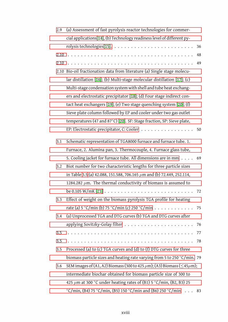
2.9 (a) Assessment of fast pyrolysis reactor technologies for commer-

cial applications[14], (b) Technology readiness level of different py-

rolysis technologies[15]. . . . . . . . . . . . . . . . . . . . . . . . . 36

2.10 . . . . . . . . . . . . . . . . . . . . . . . . . . . . . . . . . . . . . . 48

2.10 . . . . . . . . . . . . . . . . . . . . . . . . . . . . . . . . . . . . . . 49

2.10 Bio-oil fractionation data from literature (a) Single stage molecu-

lar distillation [16]; (b) Multi-stage molecular distillation [17]; (c)

Multi-stage condensation systemwith shell and tubeheat exchang-

ers and electrostatic precipitator [18]; (d) Four stage indirect con-

tact heat exchangers [19]; (e) Two stage quenching system [20]; (f)

Sieve plate column followed by EP and cooler under two gas outlet

temperatures (47 and 87◦C) [20]. SF: Stage fraction, SP: Sieve plate,

EP: Electrostatic precipitator, C: Cooler . . . . . . . . . . . . . . . . 50

3.1 Schematic representation of TGA8000 furnace and furnace tube. 1.

Furnace, 2. Alumina pan, 3. Thermocouple, 4. Furnace glass tube,

5. Cooling jacket for furnace tube. All dimensions are in mm . . . . 69

3.2 Biot number for two characteristic lengths for three particle sizes

in Table 3.5 (a) 42.088, 151.588, 706.165 µm and (b) 72.449, 252.114,

1284.282 µm. The thermal conductivity of biomass is assumed to

be 0.105 W/mK [21] . . . . . . . . . . . . . . . . . . . . . . . . . . . 72

3.3 Effect of weight on the biomass pyrolysis TGA profile for heating

rate (a) 5 ◦C/min (b) 75 ◦C/min (c) 250 ◦C/min . . . . . . . . . . . . 75

3.4 (a) Unprocessed TGA and DTG curves (b) TGA and DTG curves after

applying Sovitzky-Golay filter . . . . . . . . . . . . . . . . . . . . . 76

3.5 . . . . . . . . . . . . . . . . . . . . . . . . . . . . . . . . . . . . . . 77

3.5 . . . . . . . . . . . . . . . . . . . . . . . . . . . . . . . . . . . . . . 78

3.5 Processed (a) to (c) TGA curves and (d) to (f) DTG curves for three

biomass particle sizes and heating rate varying from 5 to 250 ◦C/min. 79

3.6 SEM images of (A1, A2) Biomass (300 to 425µm); (A3) Biomass (≤45µm);

intermediate biochar obtained for biomass particle size of 300 to

425 µm at 300 ◦C under heating rates of (B1) 5 ◦C/min, (B2, B3) 25◦C/min, (B4) 75 ◦C/min, (B5) 150 ◦C/min and (B6) 250 ◦C/min . . . 83

xviii

3.7 SEM images of biochar obtained at the end of TGA program with

heating rate (A1) 25 ◦C/min, (A2) 75 ◦C/min, (A3) 150 ◦C/min, (A4)

250 ◦C/min; intermediate biochar obtained for biomass particle size

of 300 to 425 µm at 300 ◦C under heating rates of (A5) 75 ◦C/min,

(A6) 250 ◦C/min; optical microscope image for biochar obtained

at the end of TGA program with heating rate of 150 ◦C/min for

biomass particle size of (A7) 300 to 425 µm and (A8)≤45µm . . . . 85

3.8 . . . . . . . . . . . . . . . . . . . . . . . . . . . . . . . . . . . . . . 86

3.8 Optical microscope images of particles before and after pyrolysis

(a) Biomass, 300 to 425 µm, (b) Biochar obtained at 5 ◦C/min, (c)

Biochar obtained at 250 ◦C/min. . . . . . . . . . . . . . . . . . . . . 87

3.9 . . . . . . . . . . . . . . . . . . . . . . . . . . . . . . . . . . . . . . 89

3.9 Isoconversion method plots for three particle sizes. Variation of

activation energy with respect to extent of reaction. . . . . . . . . 90

3.10 . . . . . . . . . . . . . . . . . . . . . . . . . . . . . . . . . . . . . . 92

3.10 . . . . . . . . . . . . . . . . . . . . . . . . . . . . . . . . . . . . . . 93

3.10 (a) to (c) Isoconversionmethod plots for three particle sizes. Varia-

tion of Frequency factor with respect to activation energy. (d) to (f)

Isoconversionmethod plots for three particle sizes. Linearity plots

for ln(d(α)/dt) vs. (1/T) . . . . . . . . . . . . . . . . . . . . . . . . 94

3.11 . . . . . . . . . . . . . . . . . . . . . . . . . . . . . . . . . . . . . . 95

3.11 . . . . . . . . . . . . . . . . . . . . . . . . . . . . . . . . . . . . . . 96

3.11 (a to c) Comparison of experimental and Model reaction plots for

Eq. 3.3. (d to f) Model reaction plots for different reaction models

for Eq. 3.3 . . . . . . . . . . . . . . . . . . . . . . . . . . . . . . . . 97

3.12 . . . . . . . . . . . . . . . . . . . . . . . . . . . . . . . . . . . . . . 99

3.12 . . . . . . . . . . . . . . . . . . . . . . . . . . . . . . . . . . . . . . 100

3.12 . . . . . . . . . . . . . . . . . . . . . . . . . . . . . . . . . . . . . . 101

3.12 . . . . . . . . . . . . . . . . . . . . . . . . . . . . . . . . . . . . . . 102

3.12 Comparison of experimental and predicted plots for α, dα/dt and

d2α/dt2 using objective function in (a) to (c) case 1, (d) to (f) case

2, and (g) to (i) case 3 . . . . . . . . . . . . . . . . . . . . . . . . . . 103

xix

3.13 . . . . . . . . . . . . . . . . . . . . . . . . . . . . . . . . . . . . . . 106

3.13 Conversion plots for three reaction models calculated using three

different set of DAEM parameters in Table 3.11, (a) For set no. 1, (b)

For set no. 2, (c) For set no. 3. . . . . . . . . . . . . . . . . . . . . . 107

3.14 Profile of (dα/dt)max with respect to heating rate for three particle

sizes. . . . . . . . . . . . . . . . . . . . . . . . . . . . . . . . . . . . 107

3.15 . . . . . . . . . . . . . . . . . . . . . . . . . . . . . . . . . . . . . . 113

3.15 . . . . . . . . . . . . . . . . . . . . . . . . . . . . . . . . . . . . . . 114

3.15 Characteristic time values corresponding to 90% conversion for

three particle sizes calculated using theDAEMparameters obtained

for (a) to (c) Case 2A and (d) to (f) Case 2B . . . . . . . . . . . . . . 115

3.16 . . . . . . . . . . . . . . . . . . . . . . . . . . . . . . . . . . . . . . 117

3.16 . . . . . . . . . . . . . . . . . . . . . . . . . . . . . . . . . . . . . . 118

3.16 . . . . . . . . . . . . . . . . . . . . . . . . . . . . . . . . . . . . . . 119

3.16 . . . . . . . . . . . . . . . . . . . . . . . . . . . . . . . . . . . . . . 120

3.16 Comparisonof experimental andpredicted curves for different heat-

ing rates. Predicted curves are obtained by using optimized DAEM

parameters for (a) Case 2 (b) Case 2A and (c) Case 2B . . . . . . . . . 121

3.17 . . . . . . . . . . . . . . . . . . . . . . . . . . . . . . . . . . . . . . 123

3.17 . . . . . . . . . . . . . . . . . . . . . . . . . . . . . . . . . . . . . . 124

3.17 . . . . . . . . . . . . . . . . . . . . . . . . . . . . . . . . . . . . . . 125

3.17 . . . . . . . . . . . . . . . . . . . . . . . . . . . . . . . . . . . . . . 126

3.17 . . . . . . . . . . . . . . . . . . . . . . . . . . . . . . . . . . . . . . 127

3.17 Prediction of TGA curves using F1, DP and A2 reaction models for

(a) to (c) pine, (d) to (f) pine nut shell, (g) to (i) rice husk and (j) to

(l) straw pyrolysis under 1000 ◦C/s . . . . . . . . . . . . . . . . . . 128

4.1 Pseudo components used to model biomass pyrolysis kinetics . . . 133

4.2 Representative chemical structure of ligninwithdifferent bond link-

ages [22] . . . . . . . . . . . . . . . . . . . . . . . . . . . . . . . . . 134

4.3 Combiningbiomass pseudo components into threemixtures- RM-1,

RM-2, and RM-3 [10]. The scatter points in figure (a) shows compo-

sition of different softwood, hardwood, and grass biomass species. . 135

xx

4.4 Different free radical reactions for lignin . . . . . . . . . . . . . . . 145

4.5 Correction factor profile with respect to heating rate . . . . . . . . 149

4.6 . . . . . . . . . . . . . . . . . . . . . . . . . . . . . . . . . . . . . . 160

4.6 . . . . . . . . . . . . . . . . . . . . . . . . . . . . . . . . . . . . . . 161

4.6 Comparisonof experimental [23] andpredicted values of total volatile

evolution profile of rice straw, rice husk, and pine nutshell for four

model systems . . . . . . . . . . . . . . . . . . . . . . . . . . . . . 162

4.7 . . . . . . . . . . . . . . . . . . . . . . . . . . . . . . . . . . . . . . 164

4.7 Predicted profiles of reactants and intermediates for Ranzi and M1

model systems for rice husk . . . . . . . . . . . . . . . . . . . . . . 165

4.8 . . . . . . . . . . . . . . . . . . . . . . . . . . . . . . . . . . . . . . 167

4.8 . . . . . . . . . . . . . . . . . . . . . . . . . . . . . . . . . . . . . . 168

4.8 . . . . . . . . . . . . . . . . . . . . . . . . . . . . . . . . . . . . . . 169

4.8 . . . . . . . . . . . . . . . . . . . . . . . . . . . . . . . . . . . . . . 170

4.8 Comparison of experimental [24] and predicted values of tar, gas,

and solid yield for spruce, oak and pine under 1000◦C/s and 598,

723, and 798 K. The ash content of all biomass samples is≤1 . . . . 171

4.9 Comparison of conversion time for M1, M2, M3, and Ranzi model

systems for spruce at 450◦C . . . . . . . . . . . . . . . . . . . . . . 172

5.1 Schematic of Pyrolysis BFB Model . . . . . . . . . . . . . . . . . . . 184

5.2 Flow regime diagram for gas-solid contacting . . . . . . . . . . . . 186

5.3 (a) Flowpatterns in bubblingfluidized bed reactor, (b) Tank is series

engineering model for bubbling fluidized bed reactor . . . . . . . . 187

5.4 Solution methodology for BFB reaction engineering model . . . . . 198

5.5 Volume averaged temperature profile of biomass particle for eight

different reactor temperatures. Physical properties for pine wood

used for the simulations are, density (ρ): 500 kg/m3; thermal con-

ductivity (k): 0.134 W/m/K . . . . . . . . . . . . . . . . . . . . . . 200

5.6 Dynamic response of BFB reaction engineering model for bio-char

mass fraction in emulsion and cloud cells. . . . . . . . . . . . . . . 201

xxi

5.7 Comparison between experimental and BFB reaction engineering

model results for (a) Organics andwater, (b) Gas and char products.

The experimental data is taken from [25]. . . . . . . . . . . . . . . 203

5.8 . . . . . . . . . . . . . . . . . . . . . . . . . . . . . . . . . . . . . . 204

5.8 Comparison between yields of different solid product for Case 1 and

Case 2. . . . . . . . . . . . . . . . . . . . . . . . . . . . . . . . . . . 205

5.9 . . . . . . . . . . . . . . . . . . . . . . . . . . . . . . . . . . . . . . 207

5.9 . . . . . . . . . . . . . . . . . . . . . . . . . . . . . . . . . . . . . . 208

5.9 Comparison between mole fractions of different pyrolysis gaseous

species for experiment, Case 1 and Case 2. . . . . . . . . . . . . . . 209

5.10 . . . . . . . . . . . . . . . . . . . . . . . . . . . . . . . . . . . . . . 211

5.10 Lumped yields of liquid components for Case 1 and Case 2. . . . . . 212

6.1 Approach to fractional condensation of bio-oil . . . . . . . . . . . . 217

6.2 (a) Multi-stage condensation scheme in [26] (b) Modified scheme

for validation of AspenPlus simulations . . . . . . . . . . . . . . . . 218

6.3 Quantitative distribution of fractions and chemical families in bio-

oil obtained at 400◦C in [26] . . . . . . . . . . . . . . . . . . . . . . 219

6.4 Experimental and predicted binary interaction parameters for set

of model compounds used in this study. Serial numbers in this fig-

ure sequentially represent components in Table 6.1 . . . . . . . . . 221

6.5 Condensation schemes for simulation of multi-stage condensation

of bio-oil model compounds. IDHE stands for indirect contact heat

exchanger. SEP stands for flash separators. Spray tower uses water

as a direct contact heat exchange medium. . . . . . . . . . . . . . . 222

6.6 Comparison of experimental and predicted values of bio-oil frac-

tions collected in SF1-2, SF3-4 and SF5 stages of condensation train

using (a)NRTL-NTHand (b)UNIQUAC-NTHphase equilibriummod-

els. . . . . . . . . . . . . . . . . . . . . . . . . . . . . . . . . . . . . 224

6.7 . . . . . . . . . . . . . . . . . . . . . . . . . . . . . . . . . . . . . . 225

xxii

6.7 Error between experimental and predicted value when UNIQUAC

parameters are varied within a range of ±40% of the parameter’s

original value. (Acids: Carboxylic acid, DMP: dimethoxyphenol,

Fur: Furans, LVG: Levglucosan, MMP: monomethoxyphenol, ToP:

total phenols, ToS: total sugars, Wtr: Water, Wtr Ins: Water insol-

ubles) . . . . . . . . . . . . . . . . . . . . . . . . . . . . . . . . . . 226

6.8 . . . . . . . . . . . . . . . . . . . . . . . . . . . . . . . . . . . . . . 228

6.8 . . . . . . . . . . . . . . . . . . . . . . . . . . . . . . . . . . . . . . 229

6.8 . . . . . . . . . . . . . . . . . . . . . . . . . . . . . . . . . . . . . . 230

6.8 Sensitivity studyof concentrationofmodel compoundsused to rep-

resent bio-oil. . . . . . . . . . . . . . . . . . . . . . . . . . . . . . . 231

6.9 . . . . . . . . . . . . . . . . . . . . . . . . . . . . . . . . . . . . . . 232

6.9 . . . . . . . . . . . . . . . . . . . . . . . . . . . . . . . . . . . . . . 233

6.9 . . . . . . . . . . . . . . . . . . . . . . . . . . . . . . . . . . . . . . 234

6.9 . . . . . . . . . . . . . . . . . . . . . . . . . . . . . . . . . . . . . . 235

6.9 Separation factors of chemical families in different liquid streams

obtained for scheme 1 . . . . . . . . . . . . . . . . . . . . . . . . . 236

6.10 . . . . . . . . . . . . . . . . . . . . . . . . . . . . . . . . . . . . . . 239

6.10 Relative volatility dependence of model components . . . . . . . . 240

6.11 Scheme 1 yield and purity of chemical families under optimal oper-

ating conditions for differentmass ratios of NCG: condensible com-

ponents . . . . . . . . . . . . . . . . . . . . . . . . . . . . . . . . . 242

6.12 Scheme 2 yield and purity of chemical families under optimal op-

erating conditions . . . . . . . . . . . . . . . . . . . . . . . . . . . 245

6.13 Comparison of scheme 1 and scheme 2 for chemical family yields

in each condenser. . . . . . . . . . . . . . . . . . . . . . . . . . . . 247

A.1 . . . . . . . . . . . . . . . . . . . . . . . . . . . . . . . . . . . . . . 259

A.1 . . . . . . . . . . . . . . . . . . . . . . . . . . . . . . . . . . . . . . 260

A.1 . . . . . . . . . . . . . . . . . . . . . . . . . . . . . . . . . . . . . . 261

A.1 Experimental values of α for biomass particle size less than 45 µm . 262

A.2 . . . . . . . . . . . . . . . . . . . . . . . . . . . . . . . . . . . . . . 263

A.2 . . . . . . . . . . . . . . . . . . . . . . . . . . . . . . . . . . . . . . 264

xxiii

A.2 . . . . . . . . . . . . . . . . . . . . . . . . . . . . . . . . . . . . . . 265

A.2 Experimental values of dα/dt for biomass particle size less than 45

µm . . . . . . . . . . . . . . . . . . . . . . . . . . . . . . . . . . . . 266

A.3 . . . . . . . . . . . . . . . . . . . . . . . . . . . . . . . . . . . . . . 267

A.3 . . . . . . . . . . . . . . . . . . . . . . . . . . . . . . . . . . . . . . 268

A.3 . . . . . . . . . . . . . . . . . . . . . . . . . . . . . . . . . . . . . . 269

A.3 Experimental values of α for biomass particle size between 75 to

106 µm . . . . . . . . . . . . . . . . . . . . . . . . . . . . . . . . . 270

A.4 . . . . . . . . . . . . . . . . . . . . . . . . . . . . . . . . . . . . . . 271

A.4 . . . . . . . . . . . . . . . . . . . . . . . . . . . . . . . . . . . . . . 272

A.4 . . . . . . . . . . . . . . . . . . . . . . . . . . . . . . . . . . . . . . 273

A.4 Experimental values of dα/dt for biomass particle size between 75

to 106 µm . . . . . . . . . . . . . . . . . . . . . . . . . . . . . . . . 274

A.5 . . . . . . . . . . . . . . . . . . . . . . . . . . . . . . . . . . . . . . 275

A.5 . . . . . . . . . . . . . . . . . . . . . . . . . . . . . . . . . . . . . . 276

A.5 . . . . . . . . . . . . . . . . . . . . . . . . . . . . . . . . . . . . . . 277

A.5 Experimental values of α for biomass particle size between 300 to

425 µm . . . . . . . . . . . . . . . . . . . . . . . . . . . . . . . . . 278

A.6 . . . . . . . . . . . . . . . . . . . . . . . . . . . . . . . . . . . . . . 279

A.6 . . . . . . . . . . . . . . . . . . . . . . . . . . . . . . . . . . . . . . 280

A.6 . . . . . . . . . . . . . . . . . . . . . . . . . . . . . . . . . . . . . . 281

A.6 Experimental values of dα/dt for biomass particle size between 300

to 425 µm . . . . . . . . . . . . . . . . . . . . . . . . . . . . . . . . 282

xxiv

List of Tables

2.1 Compositionof cellulose, hemicellulose and lignin for different kinds

of LCB [27] . . . . . . . . . . . . . . . . . . . . . . . . . . . . . . . . 11

2.2 Types of pyrolysis processes . . . . . . . . . . . . . . . . . . . . . . 14

2.3 Bio-oil characteristics as compared to mineral oil . . . . . . . . . . 37

2.4 Bio-oil composition for three biomass species. Composition is rep-

resented aswt.%of organic fractionof bio-oil. Water content (wt.%

dry biomass) for (a) rice straw: 22.18; eucalyptus wood: 18; pine

wood: 8.32 . . . . . . . . . . . . . . . . . . . . . . . . . . . . . . . . 39

2.5 Summary of bio-oil fractionation systems . . . . . . . . . . . . . . 46

3.1 Isoconversion or Model Free methods for kinetic analysis of TGA

curve . . . . . . . . . . . . . . . . . . . . . . . . . . . . . . . . . . 59

3.2 Kinetic models used in the solid-state kinetics . . . . . . . . . . . . 62

3.3 TGA temperature calibration parameters valid for heating rates of

5-250 ◦C/min . . . . . . . . . . . . . . . . . . . . . . . . . . . . . . 68

3.4 Non-isothermal TGA program for biomass pyrolysis . . . . . . . . . 69

3.5 Particle Size Distribution of biomass. D(v,0.1), D(v,0.5) and D(v,0.9)

is the particle size below which 10, 50 and 90 vol.% of the sample lies 71

3.6 Elemental analysis and ash content of biomass. ∗Oxygen content

was calculated by difference. . . . . . . . . . . . . . . . . . . . . . 73

3.7 Solid Residue left after pyrolysis of biomass, with different parti-

cle size, under pre-defined linear heating rate programs. Values

in parenthesis are obtained after subtracting the ash content from

the solid residue. . . . . . . . . . . . . . . . . . . . . . . . . . . . . 80

3.8 PercentMassReactedwith respect to temperature at different heat-

ing rates for different particle sizes . . . . . . . . . . . . . . . . . . 82

xxv

3.9 Details for different cases used for DAEM parameter optimization. . 91

3.10 Optimized DAEM parameters for a same initial guess value for Op-

tion 1: J1 is objective function, Option 2: mean of J1 and J2 is objec-

tive function, Option 3: mean of J1, J2 and J3 is objective function . 104

3.11 DAEMparameters derivedusing three different reactionmodels for

pyrolysis of biomass having particle size≤45µm. Parameters in set

number, (1) derived for DP, (2) derived for F1, (3) derived for A2 . . 104

3.12 Optimized DAEM parameters for three particle sizes for Case 1, 1A

and 1B . . . . . . . . . . . . . . . . . . . . . . . . . . . . . . . . . . 108

3.13 Optimized DAEM parameters for three particle sizes for Case 2, 2A

and 2B . . . . . . . . . . . . . . . . . . . . . . . . . . . . . . . . . . 109

3.14 Optimized DAEM parameters for three particle sizes for Case 3, 3A

and 3B . . . . . . . . . . . . . . . . . . . . . . . . . . . . . . . . . . 110

3.15 DAEM parameters optimized for three reaction models using py-

rolysis curves obtained for biomass particle size between 75 to 106

µm at heating rates between 150 to 250 ◦C/min . . . . . . . . . . . 122

4.1 Estimated values of biomass pseudo-components of four biomass

species usingRanzimodel characterization. Thepseudo-component

composition is reported in mole fraction . . . . . . . . . . . . . . . 136

4.2 Ranzi model for biomass pyrolysis [27] . . . . . . . . . . . . . . . . 140

4.3 Modified Ranzi model coupled with DAEM for biomass pyrolysis . . 151

4.4 List of species used in the Ranzi and modified Ranzi model. . . . . . 156

4.5 Optimized DAEM parameters and correction factor coefficients . . 158

4.6 Comparison of experimental [28] and predicted values of ash-free

cellulose pyrolysis products for M1, M2, M3, and Ranzi models . . . 175

4.7 Comparison of experimental [28] and predicted values of cellulose

(with 5 wt% switchgrass ash) pyrolysis products for M1, M2, M3,

and Ranzi models. *Char yield is for 1 wt% switchgrass ash . . . . . 176

4.8 Comparison of experimental [28] and predicted values of ash-free

hemicellulose pyrolysis products for M1, M2, M3, and Ranzi mod-

els. *Water content was not determined experimentally but is a

theoretical prediction [28] . . . . . . . . . . . . . . . . . . . . . . . 177

xxvi

4.9 Comparison of experimental [28] and predicted values of hemicel-

lulose (with 5 wt% switchgrass ash) pyrolysis products for M1, M2,

M3, and Ranzi models. *Water content was not determined exper-

imentally but is a theoretical prediction [28] . . . . . . . . . . . . . 177

4.10 Comparison of experimental [28] and predicted values of ash-free

lignin pyrolysis products for M1, M2, M3, and Ranzi models. *Wa-

ter content was not determined experimentally but is a theoretical

prediction [28] . . . . . . . . . . . . . . . . . . . . . . . . . . . . . 179

4.11 Comparisonof experimental [28] andpredicted values of lignin (with

5 wt% switchgrass ash) pyrolysis products for M1, M2, M3, and

Ranzi models. *Water content was not determined experimentally

but is a theoretical prediction [28] . . . . . . . . . . . . . . . . . . . 180

5.1 Simulation parameters for model validation. Nitrogen is used as

fluidizing gas for all the simulations. The reactor geometry and

operating conditions used in the present study are adopted form [25]199

5.2 Predicted yields of pyrolysis liquid components for Case 1 and Case

2 using BFB reaction engineeringmodel. *The columns correspond

to Case 2. . . . . . . . . . . . . . . . . . . . . . . . . . . . . . . . . 213

6.1 Composition of representative model compounds of bio-oil for As-

penPlus validation study and simulations. Bio-oil mass flow rate of

. . . . . . . . . . . . . . . . . . . . . . . . . . . . . . . . . . . . . . 220

6.2 Classification of model compounds into groups . . . . . . . . . . . 220

6.3 Operating conditions for multi-stage condensation schemes . . . . 221

6.4 Liquid yield and purity of components for scheme 1 under opti-

mized operating conditions for NCG: condensible ratio of 2.87 . . . 237

6.5 Effect of NCG: Condensiblemass ratio on yield of each bio-oilmodel

component . . . . . . . . . . . . . . . . . . . . . . . . . . . . . . . 244

6.6 Liquid yield and purity of components for scheme 2 under opti-

mized operating conditions for NCG: condensible ratio of 2.87 . . . 249

B.1 Yield and purity of bio-oil model components for scheme 1 for dif-

ferent NCG:condensible mass ratio. . . . . . . . . . . . . . . . . . . 284

xxvii

B.2 Yield and purity of bio-oil model components for scheme 2 for dif-

ferent NCG:condensible mass ratio. . . . . . . . . . . . . . . . . . . 289

xxviii

Abbreviations

A2 Avrami-Erofeev nucleation model

ACAC acetic acid

BFB bubbling fluidized bed

Cell cellulose

CellA active cellulose

CF chemical family

CFB circulating fluidized bed

CPD chemical percolation devolatilization

DAEM distributed activation energy model

DAXP dianhydro xylo-pyranose

DP depolymeriation reaction model

DTG differential thermal gravimetric data/ curve

ESP electro-static precipitator

F1 first order reaction model

FE2MACR sinapylaldehyde

FG-DVC functional group, depolymerization, vaporization and cross-linking

GMSW gluco-mannan soft wood

HCE1 active hemicellulose

xxix

HCE2 active hemicellulose

HMWL high molecular weight lignin

ITANN 3,5-dihydro benzofuran

LCB lignocellulosic biomass

LIG intermediate solid lignin component

LIGCC intermediate solid lignin component

LIGOH intermediate solid lignin component

LIGC lignin sub-component rich in carbon

LIGH lignin sub-component rich in hydrogen

LIGO lignin sub-component rich in oxygen

LMWC low molecular weight components

MW molecular weight

NBE number of bubble to emulsion mixing cells

NCG non-condensible gas

NRTL non-random two-liquid model

NTH Nothnagel

RCR rotating cone reactor

SF separation factor

STHE shell and tube heat exchanger

TANN tannins

TGA thermal gravimetric analysis

TGL triglycerides

UNIFAC UNIQUAC functional-group activity coefficient model

xxx

UNIQUAC universal quasichemical activity coefficient model

XYHW xylan hardwood

1

Chapter 1

Introduction

1.1 Introduction

This study addresses challenges related to fast pyrolysis kinetic modeling, reactor

modeling, and bio-oil instability. Simulation for bio-oil fractionation into distinct

chemical families, a relatively unexplored topic in the literature, has been exam-

ined in this thesis. This chapter sets the background for this work and briefly

outlines the work in each chapter.

1.2 Background

Lignocellulosic biomass (LCB) is an abundant, rich, and renewable source of car-

bon. Carbon is available in the form carbohydrate (cellulose and hemicellulose)

and phenolic polymer (lignin) which can be converted to different products using

biological, chemical, and thermo-chemical processes. The viability of conversion

processes depends on type of biomass, feedstock location, andmarket demand for

energy and chemicals. Pyrolysis and gasification are commonly adopted thermo-

chemical routes to convert LCB to fuel and chemical precursors/ products. Pyrol-

ysis process involves heating biomass particles in an inert atmosphere to 400-600◦C that leads to formation of gas, liquid (bio-oil), and solid (char) products. The

relative yield of each product is a function of temperature, heating rate, and intra-

particle and reactor vapor residence time. Under fast pyrolysis conditions where

particle (<3 mm) heating rates are of the order of 1000 ◦C/s and vapor reactor

2

residence time between 2-5 s, liquid yield is high (60-75 wt.%) [29]. Bio-oil, a mix-

ture of more than 300 compounds [30, 31], can be used for energy or as a source of

chemicals. However, pyrolysis has not gained commercial success because of com-

plex feedstock chemistry, bio-oil instability, poor fuel properties, and variation

in oil composition with change of feedstock chemistry and reaction conditions.

The multi-scale nature of these challenges is graphically represented in Figure

1.1. Computational models can help understand these multiscale processes and

help in efficient design and continuous operation of large scale pyrolysis plants.

This research focuses on modeling of fast pyrolysis process on particle and, re-

actor scale and presents a strategy to fractionally condense pyrolysis vapors into

individual chemical families.

Figure 1.1: Fast pyrolysis: A multiscale problem

Reactor design requires accurate knowledge of reaction kinetics. Principal chal-

lenges towards designing a robust reactor for pyrolysis reaction are (a) variable

biomass composition and (b) complex reaction chemistry. Chemical composi-

tion of biomass varies significantly with species type, soil and climatic conditions.

Variability in feedstock chemistry leads to significant variation in bio-oil product

composition and consequently affects manufacturing productivity. Further, py-

rolysis chemistry is a complex network of numerous series and parallel reactions.

The reactions can be broadly classified into depolymerization/volatilization reac-

tions (endothermic) and cross-linking/char (exothermic) forming reactions. Un-

der fast pyrolysis conditions, the selectivity for volatilization reactions is more

3

and therefore, bio-oil yield is higher as compared to char yield. It is challenging

to determine the exact reaction mechanism of pyrolysis and therefore, numer-

ous lumped kinetic models have been proposed in the literature [32]. A detailed

pyrolysis reaction kinetic model has also been proposed [33], which can predict

the concentration of significant bio-oil components. However, to add to the com-

plexity of reaction processes, biomass particle undergoes significant morpholog-

ical changes, like intermediate melting, and bubble formation during pyrolysis

[34, 35]. This in turn affects the evolution rate of volatiles from a biomass parti-

cle and can significantly affect the bio-oil composition. Lack of modeling studies

to account for the effect of morphological changes on volatile evolution rate and

bio-oil product profile has motivated a significant part of this research.

Bio-oil constituents react with one another because they belong to different oxy-

gen containing chemical families [36]. To address the undesirable reactive char-

acteristics of bio-oil, different strategies like catalytic up-gradation [37–40], frac-

tional and molecular distillation [16, 41, 42] and stabilizing solvent/additive ad-

dition [43–46] have been reported. Catalytic upgrading mainly involves cracking,

hydro-cracking and condensation reactions that reduce the oxygen content of the

bio-oil and convert the reactive species into stable compounds, improving the bio-

oil shelf life. However, as any catalyst is selective to one or two chemical function-

alities, the non selective components tend to degrade to gases or lead to coke for-

mation, thus, decreasing the liquid yield [47]. Fractionation of bio-oil, condensed

as a mixture from pyrolysis reactor, using distillation is constrained because the

liquid will degrade under sustained heat. Addition of solvent helps improve the

bio-oil stability over time but involves cost of the solvent as well as its separation

before final application of bio-oil. Therefore, condensing the vapors after pyroly-

sis reaction into individual chemical families would address the stability issue as

well as reduce the non-selective reactions during catalytic upgrading process of

bio-oil. Bio-oil collection systems are reported in the literature but none are de-

signed or operated to fractionally separate chemical families. Furthermore, there

are no reports on simulations for liquid collection systems using significant num-

ber ofmodel compounds to fairly represent phase equilibrium behavior of bio-oil.

This research thus, proposes a simulation strategy for fractional condensation of

4

bio-oil model compounds. The work reported here connects phenomena occur-

ring at different length scales in fast pyrolysis operation.

1.3 Motivation

Bio-oil as a whole has poor combustion properties and degrades over time [48].

Without upgradation, bio-oil fetches a low price as a fuel. Nevertheless it is a rich

source of value added chemicals that belong to aldehyde, ketone, carboxylic acid,

sugar and, phenol chemical families. Chemical like acetic acid is used as solvent

for many industrial processes. It is also used in the manufacture of inks, dyes,

plastics, pesticides, and wood glue. Phenol and its derivatives from bio-oil can be

used in manufacture of resins, polymers, antiseptics, and flavors. Aldehydes and

ketones can be used as precursors for specialty chemicals. Co-production of value

added chemicals and fuel precursors using fast pyrolysis process is an economi-

cally attractive option. However, designing a techno-economically feasible pyrol-

ysis process is a daunting task because of its numerous operating variables. The

interdependence among significant pyrolysis process variables associated with

upstream and downstream operations is summarized in Figure 1.2. A pyrolysis

plant should be capable of handling different feedstock for effective continuous

operation throughout the year. This implies that the reactor and bio-oil collection

system should be designed to maintain, more or less, constant throughput of the

desired product. However, there are several challenges associated with designing

upstream and downstream unit operations.

1.3.1 Challenges

Challenges associated with reactor design and downstream processing of fast py-

rolysis process are, (a) modeling reaction kinetics and inter-dependent physico-

chemical changes at particle scale, (b) bio-oil instability. Following are the chal-

lenges that hinder efficient pyrolysis process design:

1. Pyrolysis reaction chemistry is a combination of complex competitive reac-

tions and the reaction selectivity is a strong function of biomass composi-

tion, particle size, temperature, and heating rate. Reactions cause signifi-

5

Figure 1.2: Interdependence of upstream and downstream pyrolysis process vari-ables. The shaded area is not addressed in this work.

cant physical changes in biomass particlewhich in turn affect the rate of py-

rolysis. Modeling the inter-dependent reaction kinetics and particle scale

morphological changes (partial melting, cross-linking, and pore structure

changes) is difficult.

2. Kinetic models in the literature are unable to accurately quantify the effect

of these physico-chemical processes on the yield and composition of fast

pyrolysis products.

3. To maintain isothermal conditions at high heating rates, pyrolysis kinetics

experiments reported in the literature use biomass particle sizes which are

small and do not represent the pore structure of particle sizes used in large

scale pyrolysis reactors. Therefore, the effect of particle scale phenomena

on reaction rates is unaccounted for. This reduces the accuracy of bio-oil

yield and composition prediction.

4. Bio-oil is a mixture of different chemical families that undergo condensa-

tion reactions causing bio-oil polymerization, rendering it useless. Stabiliz-

ing bio-oil is important for its utilization as a fuel and for recovering value

added chemicals from it.

Therefore, an opportunity exists to investigate and propose new kinetic model

based on an experimental strategy which accounts for the interdependence of re-

action chemistry and physical changes on the rate of fast pyrolysis. The research

6

gaps, briefly highlighted in 1.2 also reveal that a cost effective bio-oil stabilization

process needs to be explored.

1.3.2 Research significance

The researchwork in this dissertation contributes to further understanding of, (a)

multiphase and multi-scale pyrolysis kinetics and (b) bio-oil processing. A strat-

egy for pyrolysis kinetics experiments and modeling is developed in Chapter 3.

The experiments are carried out to account for the effect of operating parameters

(particle size and heating rate) in large scale reactors while carefully maintain-

ing the conditions required for reaction rate determination. Such experimental

procedure will enable the researcher to possibly capture the effects of reaction

chemistry on biomass particle morphology and vice-versa. The selection of ki-

netic model and estimation of its parameters based on such experiments could

closely describe reaction scale and particle scale pyrolysis processes in large scale

reactors. Further, based on the results of Chapter 3, improvements to a detailed

kinetic model reported in the literature are presented in Chapter 4. The modi-

fication can increase the accuracy of predicting yield and composition of bio-oil

obtained from different lignocellulosic biomass in large scale reactors. This hy-

pothesis is tested in Chapter 5 where a reactormodel is coupledwith themodified

kinetic model and the one in literature. The comparison of results shows that the

model reported in this thesis fares better than the one in literature. Therefore,

the reaction kinetics experimental strategy and the model reported in this work

account for physico-chemical phenomena in fast pyrolysis and improve the pre-

diction accuracy of yields and composition of pyrolysis products.

Simulation methodology and results of bio-oil fractional condensation in Chap-

ter 6 can assist in designing downstream unit operations for bio-oil processing.

Separation of chemical families in bio-oil can improve its shelf life and facilitate

isolation of value added chemicals to make pyrolysis commercially viable.

7

1.4 Research Objectives

The primary aim of this work is development of a multi-scale modeling and simu-

lation strategy for effective design and operation of pyrolysis process. Following

are the objectives of the current research:

1. Tomodel the effect ofmorphological changes on biomass pyrolysis kinetics.

2. To model the effect of morphological changes on the yield of significant

bio-oil components by modifying detailed pyrolysis reaction kinetics.

3. Tomodel bubbling fluidized bed reactor to predict yield and composition of

pyrolysis products.

4. To present a simulation strategy to fractionally condense bio-oil into indi-

vidual chemical families.

1.5 Thesis Outline

The thesis is divided into 7 chapters as follows

1. Chapter 1 gives a brief introduction to the research problem alongwithmo-

tivation for research.

2. Chapter 2 discusses the basic concepts and terminologies of biomass py-

rolysis. An overview of type of pyrolysis processes, reactor configurations,

bio-oil composition and properties, and kinetic and reactor modeling is de-

scribed. The chapter is concluded with research significance and graphical

abstract of the thesis.

3. Chapter 3 discusses the effect of temperature and heating rate on the mass

loss profile and pore structure of biomass particles of different sizes. Dis-

tributed activation energy model (DAEM) is used to account for the effect

of morphology on kinetic parameters of biomass pyrolysis.

4. Chapter 4 discusses the coupling of DAEM with detailed pyrolysis kinetics

to improve the prediction ability of the primary pyrolysis products under

8

fast pyrolysis conditions. To quantify the effect of morphological changes

on reaction rate a correction factor, dependent on heating rate, is intro-

duced and combined with the frequency factor in rate expression. Litera-

ture based validation of the modified kinetic model is provided.

5. Chapter 5 describes the results of a continuous non-isothermal tanks-in-

seriesmodel of a bubblingfluidizedbed reactor for pyrolysis reactions. Mod-

ified kinetic parameters determined in chapter 4 are used to model the pri-

mary pyrolysis reactions, while the parameters for secondary gas phase re-

actions have been used from the literature. Literature validation of pyroly-

sis product profiles under different operating conditions are provided.

6. Chapter 6 presents a simulation strategy for fractional condensation of py-

rolysis vapors into individual chemical families. The results establish phase

equilibrium behavior of bio-oil which can be fairly represented using a set

of twenty-eightmodel compounds. Literature based validation of the simu-

lations is provided. A new condensation scheme is proposed to fractionally

condense bio-oil into distinct chemical families.

7. Chapter 7 summaries the research work by stating important observations

and findings followed by prospective areas of improvements for taking the

work forward.

9

Chapter 2

Literature review

2.1 Introduction

Chemical industry is the backbone of modern human civilization. Discovery of

crude oil caused an explosion of revolutionarymaterials like transportation fuels,

polymers, pharmaceuticals, other commodity, and engineering products. How-

ever, following the oil crisis in the 1970’s, biomass has gained traction as a re-

newable source for liquid fuels and chemicals. LCB is adopted as feedstock for

different biomass conversion technologies. Compared to biological process, py-

rolysis utilizes complete plant material and converts it to gas, liquid, and solid

product within seconds just by heating in the absence of oxygen. Small residence

times can facilitate decentralized pyrolysis plants to utilize biomass locally. Py-

rolysis hols promise as a potential technology to commercially produce fuels, fuel

pre-cursors and chemicals.

This chapter introduces LCB and its potential as a feedstock for thermo-chemical

conversion of biomass. Basic principles of pyrolysis on particle, reactor and pro-

cess scale are discussed. Kinetic and reactor modeling along with fractionation of

bio-oil is identified to be of particular interest. Challenges in the upstream, and

downstream pyrolysis processes are also briefly discussed. The chapter is con-

cluded with significance of the research work.

10

2.2 LCB as a renewable carbon resource

2.2.1 Chemical structure

Biomass based fuels and chemicals synthesized using LCB as a feedstock are re-

ferred to as second generation biofuels or chemicals. LCB is plant based material

made up of lignin, cellulose, hemicellulose, ash, and small proportion of lipids,

proteins, extractive and other compounds. The proportion of these constituents

varies with species type, soil, and climatic conditions [49]. The average compo-

sition of lignin, cellulose, and hemicellulose for different biomass types is shown

in Table 2.1. The proportion of oxygen varies with the relative abundance of cel-

lulose, hemicellulose and lignin. The O:C weight ratio for cellulose and hemicel-

lulose is close to 1 while that for lignin is between 0.3 to 0.4. The high oxygen

content reduces the calorific value of LCB, making it a poor choice for direct com-

bustion applications.

Table 2.1: Composition of cellulose, hemicellulose and lignin for different kindsof LCB [27]

Biomass Cellulose (wt.%) Hemicellulose (wt.%) Lignin (wt.%)Hardwoods stems 40 to 55 24 to 40 18 to 25Softwood stems 45 to 50 25 to 35 27 to 33Nut shells 25 to 30 25 to 30 30 to 40Corn cobs 45 35 15Grasses 25 to 40 35 to 50 17 to 24Wheat straw 38 25 18Rice Straw 33 26 10 to 13Leaves 15 to 20 80 to 85 0Switchgrass 45 31 12

Figure 2.1 shows a representative structure of major bio-polymers of LCB. The

three bio-polymers make up the secondary cell wall of the plant material. Cellu-

lose is a linear crystalline polymer with degree of polymerization between 10000

to 15000units. Hemicellulose in a chemically heterogeneous branched co-polymer

containing pentose and hexose sugars. The mono-saccharides include pentoses

(xylose, rhamnose, and arabinose), hexoses (glucose, mannose, and galactose),

anduronic acids (4-O-methylglucuronic, D-glucuronic, andD-galactouronic acids)

[50]. Depending on the type of biomass the relative content of these monomers

11

changes. Lignin is a cross-linked phenolic co-polymer that contributes to the

rigidity of the plant cell wall. The three primarymonomers of lignin are coniferyl

alcohol, coumaryl alcohol, and sinapyl alcohol. The plant cell wall is a composite

made up cellulose micro-fibers (bundles of 20 to 300 cellulose chains) wrapped in

hemicellulose, which are dispersed in a web of lignin polymers[51]. The length

scale of these composites is of the order of (10−8 to 10−7 m), while the size of the

polymers themselves is between (10−10 to 10−9 m) [52].

Figure 2.1: Representative chemical structure of cellulose, hemicellulose andlignin

2.2.2 Physical structure

The plant cells are arranged in a microstructure to smoothly enable various func-

tions. For example, collection of tracheid cells form a bundle of several hollow

tubes which gives rise to a porous structure having cavities (10−5 to 10−4 m) [52].

The size of the cavities varies depending on the biomass type [53]. Other suchmul-

ticellular structures combine to form the macrostructure of plant. These plants/

trees are then subjected to size reduction to give particles (10−3 to 10−2 m) that

are fed to biomass conversion reactors. Thus, heat and mass transport phenom-

ena occur over a wide length scale during biomass conversion process. Different

feedstock have different chemical and physical structure. Moreover, changes oc-

12

cur in the biomass during pyrolysis reaction. These changes pose a challenge for

reaction and particle scale modeling as discussed in the later part of this chapter.

2.2.3 Biomass conversion technologies

Plant material is the only renewable source of carbon which can be converted to

liquid fuels and chemicals. LCB, a non-food resource, can be converted to a spec-

trum of fuel, fuel pre-cursors, and platform chemicals. The conversion technolo-

gies include biological and thermo-chemical routes [54] as outlined in Figure 2.2.

Microbes can digest sugars to give alcohols and other fermentation products [30].

The sugars are made available for fermentation using enzymatic or acid hydrol-

ysis of cellulose and hemicellulose. For hydrolysis to work effectively, lignin and

polysaccharides need to be separated from one another [55]. Acid hydrolysis is

a harsh process which converts part of monomeric sugars to furfural derivatives

which are toxic to fermentationmicrobes even in small concentrations. Thus, the

selective enzymatic hydrolysis is preferred over acid treatment. Microbial diges-

tion of lignin is not possible and therefore, biomass is pre-treatedwith acid and/or

alkali to remove lignin chemically. This extra step adds to the cost of the process

[56]. Moreover, time required for completion of enzymatic hydrolysis, and subse-

quent fermentation process is between several hours to days. This leads to use of

reactors with large volumes that also require precise control over enzymatic and

fermentation reaction conditions. Further higher utilization of hemicellulose de-

rived pentose sugars is challenging as compared to glucose. Anaerobic digestion

process faces similar challenges. Carbon dioxide is a major by product of anaer-

obic digestion. Thus, carbon efficiency of the process is low. While the methane

produced during digestion can be used as an energy source, it has to be subjected

to subsequent reactions for converting it to chemicals.

Small and decentralized gasification, and fast pyrolysis facilities are feasible, how-

ever, other challenges have hampered their commercialization. Gasification reac-

tion occurs in a controlled oxygen environment to convert biomass to synthesis

gas. The reaction conditions and oxygen concentration can be altered to control

the CO:H2 ratio. The synthesis gas can then be fed to Fischer Tropsch (FT) reactor

to obtain FT-oil or other liquid chemicals. LCB under fast pyrolysis conditions is

13

Figure 2.2: LCB conversion techniques

converted predominantly to liquid as shown in Table 2.2. The work reported here

is focused on fast pyrolysis. Currently, 90% of crude oil is used for energy/trans-

portation application while 10% of it is used for synthesis of chemicals [54]. Sim-

ilarly, fast pyrolysis oil can be used a source of liquid fuel as well as a rich source

of chemicals. However, scale-up, and design of fast pyrolysis process, and sustain-

able operation of a commercial plant is very challenging. The subsequent sections

discuss various aspects of pyrolysis chemistry, kinetic and reactor modeling, and

bio-oil properties. Methodology adopted to address challenges associated with

each aspect are discussed followed by significance of this work.

Table 2.2: Types of pyrolysis processes

PyrolysisTechnology

Residencetime Temperature(◦C) Char Bio-oil Gas

Slow pyrolysis 5-30 min 400-600 <35 % <30 % <40 %Fast pyrolysis <5 sec 400-600 <25 % <75 % <20 %Flash pyrolysis <0.1 sec 650-900 <20 % <20 % <70 %

14

2.3 Fast pyrolysis of LCB

2.3.1 Multiphase and multiscale pyrolysis chemistry

Major LCB components, cellulose, hemicellulose and lignin undergo number of

scission, elimination, condensation, and cross-linking reactions, withmineralmat-

ter acting as a catalyst. Hemicellulose is a branched, and amorphous co-polymer

which degrades over 220-315◦C; cellulose being crystalline in nature degrades be-

tween 315-400◦C; and as lignin is a heterogeneous cross-linked polymer, it de-

grades over a wide range between 150-900◦C [57]. Pyrolysis reactions can be di-

vided into primary and secondary reactions. Chemical and physical changes that

occur during fast pyrolysis are represented in Figure 2.3. LCB polymers undergo

endothermic fragmentation to form low and high molecular weight oxygenates,

water, and gases. Simultaneously exothermic cross-linking reactions lead to char

formation [58–60]. Cellulose undergoes depolymerization to form active cellulose

and low temperature charring reactions to form char and gases. Active cellulose

is non-volatile and simultaneously undergoes fragmentation (formation of low

molecular weight carbonyl compounds) and transglycosylation (anhydro sugars

and oligosugars). These primary products undergo charring and cracking reac-

tions while moving out of cellulose matrix [61]. Hemicellulose pyrolysis follows a

similar mechanism but produces more char and fewer sugars as compared to cel-

lulose [62]. O-acetyl groups, pentose, and hexose sugars in hemicellulose produce

compounds like acetic acid, furfurals, hydroxy propanone, and water along with

carbon dioxide and monoxide [63, 64]. Lignin pyrolysis is a multistage process.

After an initial softening phase (160 to 190◦C), dehydration (∼200◦C), and cleav-

age of aryl-alkylether (150 to 300◦C), aliphatic side chains (∼300◦C), C-C linkages

(370-400◦C), and methoxyl groups (310 to 340◦C) [65]. Families representing pri-

mary and secondary pyrolysis products of lignin are shown in Figure 2.3. Also,

lignin produces more char and PAH as compared to hemicellulose and cellulose.

All three polymers pass through an intermediate molten phase during pyrolysis.

The extent of various primary and secondary reactions is a function of tempera-

ture, heating rate, intra-particle residence time, and mineral content. Low heat-

15

ing rates, long intra-particle residence time, and mineral matter promote char

formation reactions of cellulose, hemicellulose, and lignin [66, 59, 67, 68]. Gener-

ally, fast pyrolysis is carried out between 400 to 600◦C. Under fast pyrolysis con-

ditions high heating rates increase selectivity for endothermic reactions, conse-

quently increasing tar/liquid yield. The primary and secondary products shown

in the figure are representative of numerous bio-oil compounds. Beyond 500 ◦C,

where primary reactions are supposed to be completed, homogeneous tar crack-

ing reactions start; tar and char pre-dominantly gets converted to permanent gas

[69, 70]. Tar cracking can also be catalyzed by char at low temperatures, thereby

increasing the gas yield. Reactions are also accompanied by physical changes that

makes pyrolysis a multiphase process.

Figure 2.3: Multicomponent and multiphase nature of pyrolysis reactions.

Physical changes occurring during pyrolysis result in significant morphological

changes in pore structure of biomass particle. An intermediate liquid, composed

of oligomeric products, is formed inside the pores and on the biomass particle

surface [71–78]. Volatile products are released from biomass cell wall as a conse-

quence of bubble eruption [79, 35]. The vapors evolve as a consequence of reac-

tions occurring on a scale of 10−10 to 10−9 m. Vapors accumulate to form bubble

nuclei, that grow to order of 10−6 m [76] and rise through the intermediate liquid.

The vapors generated can travel outside the needle shaped biomass particle ei-

ther longitudinally or radially [80]. Pore structure of biomass particle undergoes

changes during pyrolysis reaction which alters the intra-particle resistance and

affects the volatile evolution profile [71, 34]. Eruption of vapor bubbles, that have

16

diameter of the order of cell wall thickness, lead to formation of open pore struc-

ture. Thus, there is a decrease in the resistance for vapor transport outside the

reacting particle. On the other hand melting as well as tar accumulation [34] can

block the pores of biomass and cause overpressure within the particle. Accumula-

tion of vapors inside the particle hampers its volatilization rate. At the same time

overpressure can cause micro-explosion of bubbles that release vapors and fine

liquid droplets [74, 81]. The ejected aerosols mainly contain ’pyrolytic lignin or

humins’,essentially partially degraded or cross-linked oligomers from cellulose,

hemicellulose, and lignin. The proportion of aerosols released decreases with in-

crease in particle size [82, 83]. As a result, changes in morphology (Figure 2.4) of

biomass can increase or decrease apparent biomass conversion rate [84] and thus,

need to be accounted for while modeling biomass pyrolysis.

Figure 2.4: Morphological changes occurring during biomass pyrolysis.

2.3.2 Biomass pyrolysis kinetic modeling

Knowledge of reaction kinetics is essential for accurate reactor design. Kinetic

model is essential to determine the yield of various pyrolysis species under differ-

ent reaction conditions. Pyrolysis reactions being complex are difficult to model

and therefore, several lumped kineticmodels have been proposed in the literature

[85–88, 2, 89, 67, 90, 5, 91, 32, 61]. Lumped models allow prediction of bio-oil, gas

and char yields. Single component lumped models do not consider the variation

in chemistry of LCB and kinetic parameters can not be applied to different feed-

stocks. To overcome this issue multi-component lumped models that treat cellu-

lose, hemicellulose, and lignin pyrolysis independent of each other are proposed.

17

Figure 2.5: Single and multicomponent multi-reaction kinetic models for biomass pyrolysis. (a) [1, 2]; (b) [3]; (c) [4]; (d) [5]; (e) [6]; (f) [7]; (g) [8]; (h) [9]; (i),(j),(k) [10]; (l) [11]; (m) [12].LVG: Levoglucosan; HAA: Hydroxyacetaldehyde; HCHO: Formaldehyde; LMWC: Low molecular weight compounds; Int: Intermediate; TG: trapped gases in metaplast γ: Stoichiometriccoefficient; i: component id

18

Suchmodels can be applied to determine pyrolysis reaction rate provided compo-

sition of these three polymers is known. However, hemicellulose and lignin struc-

ture varies based on type of LCB. Pyrolysis reactions and hence kinetic parame-

ters can change based on the type of LCB. Recently detailed mechanistic mod-

els are formulated based on insights from molecular simulations of monomers,

oligomers, and polymeric cellulose, hemicellulose and lignin [33, 92–95, 10]. Thus,

over the years several issues related to qualitative and quantitative prediction of

pyrolysis products have been addressed as kinetic models transformed from sin-

gle component single reaction tomulticomponentmulti-reaction lumpedmodels

to mechanistic models.

2.3.2.1 Single component multi-reaction lumped models

Two commonly used single component pyrolysis models for biomass are shown

in Figure 2.5 (a) and (b). Separate formation rates for pyrolysis gas, liquid and

char are introduced in the reaction mechanism. All the reactions are assumed to

follow first order reaction kinetics. Model (a) considers only primary reactions

but secondary tar cracking and charring reactions have been considered inmodel

(b) and (c). Secondary reactions do not strictly occur in the vapor phase. Biomass

can depolymerize into non-volatile component like active cellulose or into high

molecular weight tar which subsequently convert into volatiles and char. Thus,

consideration of secondary reactions in pyrolysis kinetic mechanism is important

for accurate predictions. Model (d) is based on a global kinetic scheme proposed

by Diebold [96]. Thurner and Mann proposed a single step reaction model, which

[97] is unable to qualitatively predict the pyrolysis product profileswith respect to

temperature [67]. Coupling of particle scale models with kinetic models based on

schemes (b) and (c) (Figure 2.5) [88, 2, 98] predicts quantitative trends of pyrolysis

products over a wide temperature range. But inaccurate quantitative prediction

of char does not allow model parameter extrapolation to fast pyrolysis reaction

kinetics. CFD simulations of bubbling fluidized bed reactor [99], using model (d)

19

and kinetic parameters from [100, 2], fairly predict yields for gas, char and tar un-

der fast pyrolysis conditions. But all these lumped models ((a) to (d)), make an

inherent assumption that cellulose, hemicellulose and lignin undergo similar py-

rolysis reactions. For cellulose and hemicellulose, the gas and char yields decrease

with increase in temperature while for lignin the liquid and gas yields increase at

the expense of char. Under fast pyrolysis conditions liquid and char formation

is favored at low temperature while gas formation is preferred at high temper-

atures [67]. Such single component models are therefore, specific to a biomass,

and experimental conditions employed. To overcome the variable biomass chem-

istry issue, kinetic models have been proposed for cellulose, hemicellulose and

lignin. The effect of mineral matter on the kinetics of these three polymers is also

published.

2.3.2.2 Multi-component multi reaction lumped models

Cellulose, hemicellulose and lignin polymer chemistry is significantly distinct.

The mass fraction of each polymer in LCB can be quantified. Thus, LCB pyrol-

ysis can be modeled by assuming that cellulose, hemicellulose and lignin inde-

pendently undergo thermal degradation. Several cellulose pyrolysis models have

been proposed in literature (Figure 2.5 (e) to (i)). Model (e) to (g) are lumpedmod-

els to describe cellulose pyrolysis. Model (e) does not distinguish between char

and gas and therefore can not be used to describe fast pyrolysis where gas yield

increases at the expense of volatiles and char. Model (f), proposedby Shafizadeh in

1979, uses ’active cellulose’ as an intermediate for the first time. However, it does

not take into consideration secondary reactions and lumps liquid and gas com-

ponents. Models (g) and (h) are modifications of the Shafizadeh model. The low

temperature and slow char formation reaction is introduced based on experimen-

tal results reported in these articles [66, 59]. Mok and Antal [66] pointed out that

the char yield was high in [6, 7] because of large sample size (100 to 250mg) which

led to significant volatile-solid secondary charring reactions. Further, Milosavlje-

vic et.al. [59] reported that endothermic (0.54 kJ/g) tar vaporization is preferred

at high heating rates over the exothermic (2 kJ/g) char formation reaction. They

also observed that the rate limiting step for cellulose pyrolysis shifts from high

20

activation energy (218 kJ/mol) to low activation energy (140 kJ/mol) reaction be-

yond 320◦C. The low temperature char formation is catalyzed by mineral matter.

Formation of sugars and LMWC in models (g) and (h) is attributed to transglyco-

sylation and fragmentation reaction. The selectivity for these reactions is not a

strong function of temperature but ofmineral content. In the presence of ash LVG

yield drops significantly as comped to that of LMWC. Thus, models (g) and (h) can

globally account for effect of temperature, heating rate, and mineral matter on

yields of gas, char and liquid provided the kinetic parameters are optimized for

sufficiently wide range of fast pyrolysis conditions.

2.3.2.3 Multi-component mechanistic reaction models

Models (i) to (k) are mechanistic models proposed by Prof. Ranzi’s group to de-

scribe the pyrolysis reactions. Several modifications [101–103] have been made

to the model after its initial publication [104, 105, 33] (Ranzi model). The model

used in this work is the 2017 version [10], where reactions for trapped gases, ex-

tractive components, and effect of ash have been included. The primary pyrolysis

reactions involve 50 species with (a) cellulose, (b)hemicellulose (xylan based for

hardwood and agricultural residue, and glucomannan based for soft wood LCB),

(c) oxygen (LIG-O), hydrogen (LIG-H), and carbon (LIG-C) rich lignin fractions, and

(d) triglyceride and condensed tannins (extractive) as initial LCB components. All

the reactions are first order Arrhenius type reactions. The other 42 species in-

clude bio-oil components (carbonyl, alcohol, furfural, phenol/phenol derivatives

and small oxygenates) and permanent gases along with pseudo-components rep-

resenting trapped gases. As LCB pyrolysis progresses through an intermediate liq-

uid phase, release rate volatile/gas species can be hampered due to entrapment.

Thus, out of the 29 primary pyrolysis reactions, 8 reactions describe the release of

trapped gases using first order Arrhenius type reactions. The model does not ac-

count for the interactions between cellulose, hemicellulose and lignin. The lignin

primary pyrolysis reaction model is a condensed version of detailed model pro-

posed by Faravelli et.al.[92]. Secondary reactions of volatile species are modeled

using 507 species and 20,239 reactions; and the files are available in the CHEMKIN

format. Anca-Couce et. al. [93] proposed a modification to Ranzi’s scheme by

21

introducing secondary charring reactions and validated the same with experi-

mental results obtained for conventional/slowpyrolysis infixedbed reactor [106].

Compared to original pyrolysis scheme of Ranzi et. al. [33] the modification im-

proved the char, carbonyl and alcohol yield predictions but over predicted per-

manent gas yields. However, validation for fast pyrolysis, where liquid yield is

maximum, has not been reported. Broadbelt et. al. [94, 95, 107] have proposed

and experimentally validated a detailed mechanistic model for cellulose pyroly-

sis based on the results of molecular simulations for cellulose and glucose-based

carbohydrates. The reaction model includes 342 primary pyrolysis reactions us-

ing 103 species that include intermediates, volatiles, permanent gases, and char.

Themodel predictions of 11major andminor species shows good agreement with

fast pyrolysis experiments of cellulose and glucose-based carbohydrates carried

out between 400 to 600◦C. Similar molecular simulation studies and experimen-

tal validation is required to understand the pyrolysis of lignin and hemicellulose.

Lignin is a complex heteropolymer and structural characterization of linkages and

chemical functionalities is a challenge [108, 109]. To account for every lignin py-

rolysis reaction knowledge of inter unit linkages and chemical group distribution

is required. But, lack of such detailed structural information does not allow deter-

mination of intermediate species and therefore, some reactions and species need

to be lumped. The β-O-4 (β-aryl ether) linkage commonly occurs in lignin and

makes up about 60% of all the linkages in lignin. For this reason, Faravelli et. al.

[92] used three model components LIG-C, LIGH, and LIG-O based on a β-O-4 skele-

ton to characterize the initial lignin structure. Distribution ofmethoxyl, aliphatic,

and oxygenated side groups, in each model compound is different (for example,

hardwoods contain more methoxyl groups than softwoods). Faravelli model has

been verified using non-isothermal TGA data (heating rate: 20◦C/min) for lignin

derived form different biomass species. The model does not show a good agree-

ment when compared with isothermal (550, 552, and 682 K) pyrolysis data for

lignin. Currently, however, Ranzi model is the only model capable of predicting

biomass pyrolysis oil composition.

22

2.3.2.4 Coal devolatilization model

Model (l) is based on model (m) (Figure 2.5) and stoichiometric coefficients are

assigned to char and gases to distinguish them from one another. Model (m) is a

scheme adopted by different coal devolatilization schemes, the functional group-

depolymerization, vaporization, and cross-linking (FG-DVC)model [110, 111], bio-

Flashchain [112], and bio chemical percolation devolatilization (CPD) [113, 12, 114,

115]. The FG model is used to describe the gas evolution and the elemental and

functional group composition of tar and char. DVCmodel describes the evolution

of tar and char through depolymerization, volatilization and cross-linking reac-

tions [116]. The DVC model describes coal as aromatic clusters linked by weak

and strong bridges. However, as coal and biomass are structurally very distinct,

FG model is more relevant than DVC model. The release of CO, CO2, H2O, CH4 and

tar aremodeled using evolution of FG, which are describedwith a distributed acti-

vation energy model (DAEM). Though the model provides precise time-evolution

profiles of volatiles, the FG-DVC model is only applicable to the fuels the model

was developed for [61]. In case of the BFC model, biomass is assumed to be com-

posed of cellulose and lignin like structure. The term ’bridge’ corresponds to

monomeric units of cellulose or lignin. The bridges can undergo scission to pro-

duce smaller fragments released as tar, small condensible, and gases. Tar release

is modeled using flash distillation analogy where the tar is assumed in vapor-

liquid equilibrium. On the other hand, the bridges can also cross-link to form

char. Like FG-DVC, the scission, condensation and char formation reactions are

described using DAEM. Finally, CPD model assumes that LCB is composed cellu-

lose, hemicellulose and lignin. LCB is assumed to be aromatic clusters connected

with weak and strong bridges. The parameters that describe the structure and

bridges are based on 13C-NMR experiments and general structural characteristics

of LCB. During pyrolysis the bridges undergo competitive scission and char for-

mation reactions again described by DAEM. Percolation statistics describes the

bridge breaking and size of fragments. Though the coal devolatilization kinetics

provides good insight in the secondary charring reactions it leads to considerable

ambiguity when applied to primary decomposition reactions of biomass.

23

2.3.2.5 Distributed activation energy model

An important feature of the coal devolatilization model is the use of DAEM to

describe pyrolysis reactions. DAEM describes a rate process as a combination of

probabilistic infinite parallel processes. The resistance/activation energy of each

parallel process is described by an Arrhenius type equation. Activation energies

are expressed using a probability distribution function. The contribution of each

process, out of the infinite possibilities, to the overall rate is weighed by the asso-

ciated probability of an activation energy value. Variation is activation energy of

chemical reaction can be attributed to heterogeneity of molecular environment

in a solid [117]. Multi-component DAEM has been employed in modeling biomass

pyrolysis [118–120]. Multi-component DAEM defines the overall volatilization of

biomass as a linear combination of weighted reaction rates, where the reaction of

each component is described by DAEM. A detailed derivation of the DAEM equa-

tion can be found in Chapter 3. In case of LCB, the molecular chemical compo-

sition varies spatially. Therefore, activation energy for a particular reaction can

vary depending on spatial location of the active site in LCB. For example, acti-

vation energy for cellulose fragmentation can be different when the active site

is in vicinity of hemicellulose/lignin macromolecules when compared to an ac-

tive site in vicinity of another cellulose chain. Also, presence/absence of mineral

matter in LCB matrix can affect the activation of a reaction significantly. Thus,

any one of the reaction described in mechanistic models can be described using

DAEM to take into consideration the interaction between cellulose, hemicellu-

lose, and lignin. Moreover, mechanistic models of lignin and hemicellulose are

developed for lignin and hemicellulose extracted from LCB using acid/alkali pre-

treatments. These treatments lead to structural changes in lignin and hemicellu-

lose. DAEM can thus, bridge such gaps when mechanistic models developed for

cellulose, hemicellulose, and lignin are used to model pyrolysis of whole biomass.

Further, the softening ormelting behavior of LCB components is considerably dif-

ferent as demonstrated by Dufour et. al. [76, 121]. The softening/melting be-

havior of lignin, cellulose, and hemicellulose was reported as fraction of mobile

protons present during pyrolysis using a 1H-NMR in a temperature range of 150

to 450◦C. Mobility of hydrogen begins in lignin (fluidity begins around 150◦C and

24

reaches 100% between 200-225◦C) and cellulose (fluidity begins around 250◦C) be-

fore any mass loss while that in xylan begins after some initial degradation. The

fluidity of cellulose and xylan reaches a maximum of 28% around 350◦C, and 60%

around 270◦C respectively under a heating rate of 5 K/min. The fluidity drops

after 350◦C for lignin and cellulose as a result of cross-linking char forming re-

actions. For xylan the fluidity drops after 270◦C and becomes constant at 20%

thereafter. However, for the biomass- Miscanthus, the softening begins at 200◦C

against 150◦C for isolated lignin. Moreover, themaximumfluidity achieved is 42%

which is much lower than that for lignin and xylan. The high mobility for xylan

and lignin is a result of reduction in molecular weight during their isolation from

LCB. The low mobility in native LCB also suggests strong interaction between the

threemacromolecules. Presence ofmolten phase gives biomass viscoelastic prop-

erties which change with temperature and depend on the heating rate employed

in pyrolysis. Therefore, models that describe the complex chemistry and account

for the effect of morphological changes on reaction rates can accurately simulate

pyrolysis process.

2.3.2.6 Experimental parameters for pyrolysis kinetics

The accuracy of a kineticmodel depends on howwell themodel captures different

processes occurring during pyrolysis; and the value of model parameters. Com-

monlyused apparatus for determining kinetic parameters are thermo-gravimetric

analyzer (TGA), TGA-FTIR, TGA-MS,wiremesh reactor, isothermalmicro-pyrolyzer

(Pyroprobe)/drop tube reactor coupledwithGC-MS, isothermal entrainedflowre-

actor, isothermal fixed bed reactor, and tube furnace. Sample type, sampleweight,

sample particle size, heating rate, and reactor temperature affect the value of ki-

netic parameters [67, 122, 123, 61]. The TGA data of biomass pyrolysis reported

in literature uses heating rates between 2 to 150◦C/min, sample size between 1

mg to 300 mg, and minimum and maximum particle sizes of 40 and 2000 µm

[67, 124, 78, 91]. On the other hand the heating rate in wire mesh reactor and

micro-pyrolyzer can be as high as 10000 ◦C/s with sample weight of the order of

0.1 mg and particle size less than 40 µm [62, 122, 123, 23]. Sample weight and par-

ticle size are chosen to avoid intra-particle heat and mass transfer limitations. To

25

determine if the reactions are kinetically limited, dimensionless Biot (Bi) 2.1 and

pyrolysis numbers (Py) Eq.(2.2) and Eq.(2.3) are calculated. PyI is the ratio of reac-

tion and conduction time scales, PyII is the ratio of reaction and convection time

scales, and Bi is the ratio of conduction and convection time scales. PyIII (Eq.(2.4)

ratio of conductive heat transport to reaction heat generation/consumption) and

PyIV (Eq.(2.5) ratio of convective heat transport to reaction heat generation/con-

sumption) were defined in [13] to evaluate the effect of the heat of reaction on the

intra particle temperature gradients.

Bi = hL

λ(2.1)

PyI = λ

ρCpL2kpy

(2.2)

PyII = h

ρCpLkpy

(2.3)

PyIII = λ(T∞ − T0)ρL2kpy∆H

(2.4)

PyIV = h(T∞ − T0)ρLkpy∆H

(2.5)

The external heat transfer coefficient, thermal conductivity, density, pyrolysis re-

action rate, and heat capacity of biomass are represented by h, λ, ρ, kpy, and Cp,

respectively; T∞ and T0 are the external bulk temperature of the reactor envi-

ronment and initial temperature respectively. Biomass particle size in Figure 2.6

and 2.7 is Feret diameter of the particle. Feret diameter is defined as longest dis-

tance between pair of parallel lines tangent to the largest projected particle out-

line. Biomass particle is like a rectangular parallelepiped with smooth corners.

Therefore, Feret diameter is equal to the length of the diagonal joining two edges

along the length of biomass particle. Wiggins et.al. [13] used realistic biomass

26

particle CAD geometry tomodel intra-particle thermal gradients. The volume and

surface area of particles with different Feret diameter are used to determine the

characteristic length for calculating different dimensionless numbers. Figure 2.6

shows the reaction-transport regime map for different particle sizes under for

three values of external heat transfer coefficients. Values of heat transfer coef-

ficients used are typically achieved in TGA (∼35 W/m2K), fluidized bed reactor

(∼350 W/m2K) [125], and micro-pyrolyzers (∼3500 W/m2K) [73]. It is important

to note that values of reaction rate, heat transfer coefficient, and characteristic

length can significantly affect the estimation of reaction regime. Endothermic

and exothermic regions in Figure 2.7 (a) and (b) correspond the hypothetical case

where pyrolysis reactions are either completely endothermic (only depolymeriza-

tion reactions) or completely exothermic (only charring and cracking reactions).

Assuming that the particle is at 573 K and the external temperature is 773 K, val-

ues of PyIII and PyIV decrease with increase in particle size even for Bi < 1. This

indicates that internal temperature gradients may exist within a particle as a re-

sult of heat of pyrolysis reaction. It is also important to note that biomass particle

undergoes prominent expansion and shrinkage which affects the characteristic

length of the particle and hence pyrolysis number. However, the regime diagram,

PyIII , and PyIV facilitate an estimate of particle size for conducting experiments

in the kinetically controlled and isothermal regime. Using different apparatus ex-

periments can be carried out over a wide range of heating rates. It is necessary to

ensure that appropriate sample particle size and sample weight are chosen.

TGA and wire mesh reactor can monitor weight loss as temperature increases.

The reactors can be coupled with FTIR or GC-MS to characterize the pyrolysis

products. TGA apparatus is more sensitive and accurate than the current wire

mesh reactors; but heating rates do not exceed 500◦C/min, which is much less

than heating rates employed under fast pyrolysis. Micro-pyrolyzers are operated

under isothermal conditions and biomass heats up to the reactor temperature

very rapidly. The products are then quantified continuously using GC-MS. How-

ever, biomass can not be heated to high temperature without passing through low

temperature. Biomass starts to degrade generally around 200◦C and fast pyroly-

sis temperature is ∼500◦C. Therefore, the kinetic model and parameters should

27

Figure 2.6: Reaction-transport process regime map calculated with h = 35, 350,and 3500 W/m2K, λ = 0.16 W/mK, ρ = 720 kg/m3, and Cp = 103.1 + 3.867T (J/kgK), k= 0.0622 s−1 (at T = 773 K) (figure adapted from [13]).

be capable of explaining the behavior of biomass in non-isothermal region along

with final yields of pyrolysis product composition.

Pyrolysis reaction kinetics is a strong function of biomass type, heating rate and

temperature. Selectivity of reactions changes with respect to heating rate. Cross-

linking and depolymerization reactions happen in the intermediate liquid. At low

heating rates the liquid/viscoelastic character of biomass particlemay be lost due

to high selectivity for charring reactions. On the other hand, at highheating rates,

vapors might accumulate and form bubbles like that in a viscous boiling liquid.

Though the shape of the biomass particle is maintained during pyrolysis, the pore

structure may change significantly which can significantly affect volatilization

rate. Thus, whether kinetics obtained at low heating rates can be applied at high

heating rates is a question.

2.4 Fast pyrolysis reactors

As discussed in section 2.3.2 char formation reactions are triggered at low tem-

peratures and char yield increases if biomass particle spends more time at low

28

(a)

(b)

Figure 2.7: (a) and (b) Plots for PyIII and PyIV with respect to Bi for T∞ = 773 K,T0 = 573 K, ∆ Hendo = 540kJ/kg, and ∆ Hexo = -2000kJ/kg. The particle dimensionis the Ferret diameter and it has been used in [13].

29

temperature than at high temperature. On the other hand if the generated pyrol-

ysis vapors spend more time at high temperature secondary charring and crack-

ing reactions reduce the liquid yield. Therefore, a fast pyrolysis reactor should

ensure (a) rapid heat transfer to biomass particle and (b) low vapor residence

time, to maximize the bio-oil yield. Different reactor configurations are shown

in Figure 2.8. In practice, high external medium-to-solid heat transfer rates are

required (approximately >400-500 W/m2K); intra-particle biomass heat transfer

limitation should be avoided (requiring particles <2-3 mm to limit the heat pene-

tration depth); and vapor phase residence times should be kept below a few sec-

onds in order to maintain the oil yield. Other than vapor residence time, oil com-

position can be modified by process conditions, equipment dimensions, and the

application of catalysis.

2.4.1 Rotating cone reactor

In rotating cone reactor (RCR), heat carrier particles (hot sand) and biomass par-

ticles are transported to the bottom of a conical bed Figure 2.8 (a). Centrifugal

force created by the rotating cone pushes the solid particles outwards. Thismove-

ment causes mixing of sand and biomass particles and brings the solids in contact

with heated cone surface. Generated pyrolysis vapors travel outwards towards

the condenser while the solid particles spill over top of the cone. Sand particles

are heated by char combustion and also reheated before recirculating in the re-

actor [126]. Typical conditions of RCR are, hot sand at 500◦C and cone rotation

of 300 rpm with bio-oil yield of approximately 70 wt.%. The heat transfer coeffi-

cients for rotating cone reactor are found to be of the order of 500 to 1000W/m2K,

which is high when compared to gas/solid contactors [127]. Biomass Technology

Group- Biomass to Liquid (BTG-BTL) supplied a 2 tons/hr demonstration unit to

Malaysia for converting empty fruit bunch to bio-oil in year 2004. 1000 tons of

bio-oil has been produced using 5000 tons of wet biomass (70 wt.%moisture). An-

other BTG-BTL facility constructed by Empyro BV in 2014 converts 5 tons/hr of

biomass into oil (3.2 tons/hr), process steam and electricity [128, 129].

30

Figure 2.8: Fast pyrolysis reactor configurations (a) Rotating cone ablative reactor;(b) Ablative reactor; (c) Auger reactor; (d) Circulating fluidized bed reactor; (e)Bubbling fluidized bed reactor.

31

2.4.2 Ablative reactor

In ablative pyrolysis reactor biomass is heated by pressing it against a rotating hot

disc. Pyrolysis of the biomass forms a oily layer on the disc which evaporates and

the vapors are condensed to recover bio-oil. Char produced is combusted which

heats the rotating disc [130]. Rate of reaction depends the pressure exerted on

biomass in contact with hot surface and available heat transfer area [131]. An im-

portant feature of the ablative process is that biomass undergoes ablation when

it is contacted with the hot surface. As biomass is pyrolyzed, new biomass surface

is exposed to the heated surface. Therefore, biomass particle size does not affect

the pyrolysis behavior and yield of products [132]. The limiting factor for biomass

pyrolysis is rate of heat transfer to the hot surface. Though the ablative reactors

can be compact, require small volume of condensers, and reduces biomassmilling

efforts, the following disadvantages limit the scale up of ablative reactors: (a) Heat

transfer is limited because hot surface, which is roughly at 500◦C, is heated indi-

rectly by combustion gases at 800◦C. Electric heating to compensate for heating

requirement can limit the scale up of ablative reactors, (b) restriction on biomass

particle shape to ensure its free flow since the biomass needs to be pressed against

hot surface [129]. A pilot scale ablative reactor (6 tons/day, biomass particle size

60mm x 40mm x 5mm) designed by PyTec, Germany is operating and combusting

produced oil to run 300 MWe diesel engine [15].

2.4.3 Auger reactor

Biomass undergoes pyrolysis inside a heated tube and is transported through the

length of the tube by a screw [133]. Carrier or inert gas is fed into the biomass

hopper to avoid oxidation reaction and also provide a positive pressure to trans-

port the vapors out of the reactor towards the condenser system. Sand can be

used as a heat carrier and heat transfer to the biomass particles takes place by

intimate contact with a heat carrier. The external surface of the tube can also be

heated to maintain the heating required for pyrolysis. The vapor residence time

inside the auger reactor is of the order of 5 to 30 s [126]. The oil yield in auger

reactor is between 48-62 wt.%, which is less than fluid bed reactor. Moreover,

32

water formation is enhanced (30 to 55 wt.% of bio-oil) as a result of long contact

time between char and pyrolysis vapors [131]. Renewable Oil International, USA

and AbriTech, Canada [134] have installed auger reactors with 24 tons/day and

50 tons/day capacity respectively. However, the current status of these plants is

unknown.

2.4.4 Circulating fluidized bed reactor

Bio-oil yield between 54 and 71 wt.% can be achieved using circulating fluidized

bed (CFB) reactor [135, 136]. Biomass is fed into a riser or fast fluidization sec-

tion, where extensive contacting between inert particles (sand) and biomass takes

place. Char and sand both are entrained out of the reactor, and circulated to the

regenerator where the char and coke formed on the sand is combusted. The sand

is reheated as a result of char combustion. CFB technology is widely used in the

petroleum industry for FCC process and the technology is well understood [137].

However, similar to fluid bed technology, large amounts of gas needed for fluidiza-

tion/recirculation of the reactor should be the non-condensible part of the pyrol-

ysis gas. Finally, to obtain a solid flux between 100 to 200 kg/m2s, a gas flow rate

of the order of 1000 m3/hr (ton/hr biomass) needs to be employed [135]. Such a

huge volume of non-condensible gas needs to be cooled to very low temperatures

to maximize bio-oil recovery and reheated again before it is fed to the reactor.

Ensyn has installed a 2 and 150 tons/day CFB in Canada, and VTT/Valment has in-

stalled a 15 (year 2009, pilot plant) and 274 (year 2013, commercial demonstration

plant) tons/day CFB in Finland. Ensyn plant in Ontario has a production capacity

of 11 million litre/annum of bio-oil. The bio-oil produced in the VTT/Valment

commercial demonstration plant has a heating value of 13-18 MJ/kg, 20-35 wt.%

water and a pH of 2-3. The oil is used in Fortum’s heat and power plant in Joensuu,

Finland. All these facilities are currently operational.

2.4.5 Bubbling fluidized bed reactor

Bubbling fluidized bed reactor technology is well understood and is simple in con-

struction and operation compared to other reactors. Sand is used as a heat car-

rier and is fluidized using inert gases. When the gas velocity exceeds 2 to 3 times

33

that of the minimum fluidization velocity, gas accumulates as bubbles and travels

through the fluidizing sand bed. Formation of bubbles causes solids to circulate

within the bed, thus, providing mixing. Biomass particles are generally fed from

the side into a heated bubbling bed [138]. The high solid density of bed material

and vigorous mixing induced by bubbles ensure rapid heat transfer to biomass

particles and facilitate good temperature control. Literature suggests that 2 to 3

mm of particle size is required to attain high heat transfer rates but some studies

show that a particle size of approximately 0.5 mm is required to avoid retention

of aerosols inside the particles and achieve high heating rates [82, 83]. Typical

yield of bio-oil is between 35 to 69 wt.% for grasses or agricultural residue, 59 to

79 wt.% for softwood, and 59 to 77 wt.% for hardwood [131]. Vapor and solid resi-

dence time (∼1 to 4 s) is controlled by the fluidizing gas flow rate and is higher for

char than for vapors. Char acts as an effective vapor cracking catalyst at fast py-

rolysis reaction temperatures, thus, rapid separation of char and pyrolysis vapor

is essential to avoid bio-oil reduction. Fluidizing gas velocity is adjusted such that

it can entrain char particles from the bubbling bed. However, One severe limita-

tion of bubbling fluidized bed reactor is that rate of particle heating in the bed is

usually the rate limiting step. It becomes significant for large scale reactors. Heat-

ing is generally achieved by combustion of pyrolysis gases and char and typically

transferred to the bed by internal coils and externally heating the fluidizing gas.

A coil with surface area of 10 to 20 m2 is required to convert 1 ton/hr of biomass

under fast pyrolysis conditions [135]. In 2000s DynaMotive installed 100 and 200

tons/day bubbling fluidized bed reactor in West Lorne and Guelph, Canada which

started operating in 2005 and 2006. However, due to construction and operational

issues the plants did not operate for very long [135].

Figure 2.9 (a) shows the comparison of different reactor configurations in terms

of technology strength and market attractiveness, and Figure 2.9 (b) shows the

current status of technology readiness for commercialization. Ensyn’s RTP and

BTG’s RCR technologies are used currently at commercial scale. But, bio-oil ob-

tained from commercially facilities has been primarily used for combustion or is

upgraded via hydrogenation for energy applications. Recently, it is shown that

fractionating bio-oil into individual chemical families can improve bio-oil stabil-

34

ity, facilitate efficient upgradation, and also assist in recovery value added chem-

icals from bio-oil. Using a fraction of bio-oil as a source of value added chemicals

makes pyrolysis more attractive. However, to achieve this objective it is essential

to predict pyrolysis vapor composition exiting the reactor so that downstream

operations can be designed and operated as required. As a result, one part of this

research focuses on coupling reactor hydrodynamics with detailed pyrolysis ki-

netics to predict the bio-oil composition.

2.5 Fast pyrolysis bio-oil

Fast pyrolysis vapor when rapidly quenched forms a condensate, often called bio-

oil. Bio-oil is a complexmixture of several hundred compounds [29–31] formed as

a result of rapid depolymerization and fragmentation of cellulose, hemicellulose,

and lignin. The compounds belong to a wide spectrum of chemical functionalities

namely, carboxylic acid, aldehyde, ketone, furan, carbohydrate and phenol. The

molecular weight of the compounds varies between 60 to 10000 g/mol (formed

as a consequence of aerosol ejection) [139], depending on heating rate, tempera-

ture, mineral content, and catalyst. Bio-oil instability is attributed to high oxygen

content and presence of diverse chemical functionalities. The components un-

dergo condensation polymerization reactions which are accelerated on exposure

to heat. As a result, bio-oil viscosity increases with time and can also form sepa-

rate aqueous and organic phases[140]. Unstable nature of bio-oil puts limitation

on its direct applications. However, chemical and/or physical upgradation tech-

niques can be used to produce fuel, fuel pre-cursors, intermediates, and chemi-

cals. The choice and efficiency of upgradation technique thus, strongly relies on

knowledge of bio-oil composition and characteristics.

2.5.1 Physical and chemical properties of bio-oil

Bio-oil characteristics for different biomass species are tabulated in 2.3 and com-

paredwithmineral oil properties. Substantial amount of water (biomassmoisture

and water of reaction) is present in bio-oil. The water content can be as high are

50 wt.% for agricultural residues [141] due to high ash content when compared to

35

(a)

(b)

Figure 2.9: (a) Assessment of fast pyrolysis reactor technologies for commercialapplications[14], (b) Technology readiness level of different pyrolysis technolo-gies[15].

36

forest residues. Water content lowers the calorific value of bio-oil and delays ig-

nition when compared to mineral oil. Acidic pH of bio-oil poses challenges for its

storage and combustion applications. Bio-oil consists of polar oxygenated com-

pounds which reduce its miscibility with hydrocarbon fuels. High oxygen ratio

also lowers the heating value and causes instability in pyrolysis oil. Bio-oil un-

dergoes aging through several reactions that occur amongst several hundred oxy-

genated compounds with some chemical functionalities acting as catalysts for ag-

ing reactions [142].

Table 2.3: Bio-oil characteristics as compared to mineral oil

Pyrolysis liquid Mineral oilProperty Birch Pine Poplar Range

Solids (wt.%) 0.06 0.03 0.045 0.01-1pH 2.5 2.4 2.8 2.0-3.7Water (wt.%) 18.9 17.0 18.9 15-30 0.025Density (kg/m3) 1.25 1.24 1.2 1.1-1.3 0.89Viscosity, cSt(50◦C) 28.0 28.0 13.5 13-80 6

LHV (MJ/kg) 16.5 17.2 17.4 13-18 40.3Ash (wt.%) 0.004 0.03 0.01 0.004-0.3 0.01C (wt.%) 44.0 45.7 46.5 32-49H (wt.%) 6.9 7.0 7.2 6.9-8.6O (wt.%) 49.0 47.0 46.1 44-60 0S (wt.%) 0 0.02 0.02 0-0.05 0.2Flash point (◦C) 62 95 64 50-100 60Pour point (◦C) -24 -19 -36 to -9 -15

Bio-oil components can be broadly classified into water soluble (WS) and water

insoluble (WIS) fractions. WIS fraction mainly comprises of pyrolytic lignin and

lignin monomers, while WS fraction contains low molecular weight compounds

like sugars, carboxylic acids, aldehydes, and ketones [143]. The proportion of

these fraction changes based on the biomass feedstock and reaction conditions.

Table 2.4 shows thedetailed bio-oil compositionof three different biomass species.

WS and WIS fractions undergo different aging reactions. WIS fraction result in

the formation of sticky gum like structure and cause phase separation in bio-oil

[144, 145]. On the other hand the WS fraction undergoes degradation followed

by polymerization reactions to form brown solids [146]. Components of WS and

WIS also interact with one another to promote condensation reactions in bio-oil.

Carbonyl compounds are the most reactive species present in bio-oil [147]. C-C

37

bond formation between lignin oligomers can be catalyzed by acids. Aldehydes

like formaldehyde can condense with pyrolytic lignin in presence of carboxylic

acids to form cross-linked polymers. Sugar dehydration in presence of acids re-

sults in formation of reactive furfural derivatives and levulinic acid which can self

condense or react with one another to form humins [148]. Acids also trigger self

polymerization and aldol condensation reactions in aldehydes to form oligomers

and polymers. As a result of several polymerization reactions, molecular weight

of bio-oil increases gradually with time making bio-oil useless. Thus, bio-oil as a

mixture is unstable and unsuitable formany applications; and bio-oil upgradation

or processing is essential.

38

Table2.4:Bio-oilcompositionforthreebiomassspecies.Compositionisrepresentedaswt.%

oforganicfractionofbio-oil.Watercontent(wt.%

drybiomass)for(a)ricestraw:22.18;eucalyptuswood:18;pinewood:8.32

Compounds

Ricestraw[149]Eucalyptuswood[150]Pinewood[151]

AnhydroSugars

Levoglucosan

0.7

14.75

14.20

Carboxylicacids

Aceticacid

3.16

13.02

Propanoicacid

0.86

4.14

2-Oxopropanoicacid

2.51

4-Oxopentanoicacid

1.21

propenoic

acid-3(4-hydroy-3-methoxyphenyl-)

2.25

oleicacid

0.39

3,4-dimethylbenzoicacid

0.09

Ketones

1-hydroxy-2-Propanone*

1.21

4.91

2-Butanone

1.3

1,3-Cyclopentanedione

2.45

39

Table2.4continuedfrom

previouspage

Compounds

Ricestraw[149]Eucalyptuswood[150]Pinewood[151]

2-Hydroxy-3-methyl-2-cyclopentenone

1.22

Cyclopentanone

0.27

3-methyl-1,2-Cyclopentanedione

0.09

1.00

methyl-2-Cyclopentene-1-one

0.29

1-(4-hydroxy-3-methoxyphenyl)

Ethanone

0.16

Aldehydes

Formaldehyde

0.42

Hydroxyacealdehyde

8.43

Butanedial

1.1

Ethers

2,2,4-Trimethyl-1,3-dioxalane

2.06

2,2-dimethoxypropane

1.34

Furans

Coumaran

3.08

40

Table2.4continuedfrom

previouspage

Compounds

Ricestraw[149]Eucalyptuswood[150]Pinewood[151]

Furfural

0.75

0.47

5-Methylfurfural

0.1

Furfurylalcohol

0.05

2,5-dimethoxyTetrahydro

furan

1.43

2(5H)-Furanone

0.07

4-Methyl-5H-furan-2-one

5-Methyl-2(5H)-furanone

0.16

2-(3H)-furanone,dihydro-3-hydroxy-4,4-dimethyl-

0.16

2-furanethanol,methoxy

1.59

5-Hydroxymethylfurfural

0.01

Phenols

Phenol

0.99

1.30

0.77

Cresols

2.35

0.16

1.08

Dimethylphenols

3.34

0.29

41

Table2.4continuedfrom

previouspage

Compounds

Ricestraw[149]Eucalyptuswood[150]Pinewood[151]

Guaiacol

0.79

0.27

0.39

Methylguiacols

0.83

0.11

0.54

Eugenols

0.39

1.16

0.81

Benzenediol

1.28

Methylbenzenediols

1.63

3.09

Vanillins

3.32

0.24

2,5-dimethoxy-4-ethyl

benzaldehyde

0.70

Syringaldehyde

2.64

4-Allylsyringol

2.20

Hydroquinone

0.20

Aromatics

Stilbene

0.27

Polyaromatics

0.02

Naphthalene

0.02

42

Table2.4continuedfrom

previouspage

Compounds

Ricestraw[149]Eucalyptuswood[150]Pinewood[151]

Sulphurcompounds

diBenzothiophene

0.39

Unidentified

9.59

33.86

58.32

TotalIndividualcom

pounds

35.18

66.14

41.68

43

2.5.2 Catalytic upgradation of bio-oil

Pyrolysis oil can be upgraded using several chemical and physical processes like

catalytic deoxygenation/ hydro-deoxygenation (HDO), cracking/ hydro-cracking,

esterification, steam reforming, gasification, fractionation, and emulsification.

Catalytic upgrading mainly removal of oxygen from bio-oil and converting the

reactive species into stable compounds, to improve bio-oil shelf life. Zeolites and

metal ion impregnated zeolites are generally used as catalysts for cracking or

hydro-cracking reactions. These reactions are carried out at temperatures rang-

ing from 300 to 600◦C, and in presence/absence of hydrogen [152, 126]. The main

products are oxygen devoid aromatic compounds and light hydrocarbon gases.

HDO employs supported catalysts like Pt/Al2O3/SiO2, Rh/ZrO2, CoMoS2/Al2O3,

and NiMoS2/Al2O3 [153, 154] under pressures of 75 to 300 bar and temperatures

of 250 to 400◦C. However, any catalyst is selective to one or two chemical func-

tionalities, the non-selective components tend to degrade to gases or lead to coke

formation, thus, decreasing the liquid yield and deactivating the catalyst [47]. For

zeolite upgrading and HDO, coke formation is a pronounced problem. Formation

of catalytic coke is attributed to accumulation, and polymerization and polycon-

densation of high molecular weight aromatic moieties of bio-oil on catalyst sur-

face[152]. Compounds that have more than one oxygen atom appear to have a

higher affinity for carbon formation [155]. Further, typical liquid yields after ze-

olite and HDO upgradation are 12-28 and 21-65 wt.% of bio-oil feed respectively.

Other catalytic upgrading techniques involve ketonization, condensation, hydro-

genation of carbonyl group, and hydrogenation of furanyl rings. However, these

techniques are very selective and often catalyst suffer from poisoning and deacti-

vation due to the presence of non-selective components [47]. Therefore, employ-

ing bio-oil as a mixture to upgradation leads to undesirable carbon loss.

2.5.3 Fractional condensation of pyrolysis vapors

To address bio-oil instability and storage issues, pyrolysis oil is collected in mul-

tiple condensers to concentrate bio-oil fractions having different physical and

chemical properties [156, 157, 20, 26, 19, 158, 159]. Results of multi-stage conden-

44

sation systems are tabulated in Table 2.5. Bio-oil components have awide range of

molecular weight and boiling point. The condenser temperature, residence time

of vapors and carrier gas velocity affect liquid recovery and aerosol carry-over.

Series of indirect and direct contact heat exchangers and, electrostatic precipita-

tors (ESP) are widely used for stage-wise condensation of pyrolysis vapors.

Figure 2.10 shows the composition of liquid collected in different stages of var-

ious condensation systems. Single and multi-stage molecular distillation result

in 70 to 80% of water being distilled out in the first stage. Single stage distilla-

tion better separates carbonyl compounds and acids from phenol derivatives and

sugars. Acids get concentrated in light fraction for single stage molecular distil-

lation (Figure 2.10 (a)) while they are distributed approximately evenly in all frac-

tions as shown in Figure 2.10 (b). The second strategy opted to improve bio-oil

combustion and storage characteristics is fractionally condensing pyrolysis va-

pors in multiple condensers (Figure 2.10 (c) to (f)). The standard condensation

scheme employed is a train of indirect contact heat exchangers. Factors affect-

ing condensation of chemical families are condenser temperature, proportion of

non-condensible gases, partial pressure of a component, and vapor-liquid inter-

action amongst different species. Use of multiple stages and low condenser tem-

peratures does not allow separation amongst chemical families (Table 2.5, frac-

tionation system no. 3, 6, 7, 8). Partial pressure of components can be altered

to enhance the separation amongst chemical families/compounds by altering the

amount of carrier/sweeping gas flow rate [160]. However, increasing the carrier

gas flow rate can increase aerosols carry over. Aerosol carry over is significant

when bubbling fluidized bed reactors are used for pyrolysis. Presence of sugars

and pyrolytic lignin in stage 2 and 3 (Figure 2.10 (c)) is evidence of significant

aerosol carry over. Therefore, ESP’s are used to capture the fine droplets. Spray

towers/ direct contact condensers are used to quench pyrolysis vapors to avoid

secondary reactions thus, maximizing bio-oil recovery (Figure 2.10 (e)). Studies of

multi-stage condensation have only focused on separating water and acids from

rest of the organic components of bio-oil to improve its stability and combus-

tion properties. Effective separation amongst chemical families is not achieved

in reported condensation schemes. Westerhof et.al. [156] studied the effect of

45

Table 2.5: Summary of bio-oil fractionation systems

Fractionationsystem Reaction conditions

Fractionation system operatingconditions Outlet vapor temperature Outcomes Reference

Single stagemolecular distillation

Reactor: 1 kg/hr bubblingfluidized bed, 450 to 500◦C

Pressure: 60 Pa, evaporator temperature: 70◦C,cooling jacket: 20◦C. Fraction remaining in theevaporator is heavy cut; fraction collected at20◦C is medium cut; and fraction notcondensed at 20◦C is the light cut

Bio-oil recovery is close to 85%. Light fraction is mostly waterwith high acidity and least stability.Though more than 70% ofacids, aldehydes, ketones, phenols and guaiacols from whole bio-oilare present in light fraction, molecular distillation does not alloweffective separation amongst chemical families in single stage.

[16]

Multi-stagemolecular distillation

Reactor: 5 kg/hr bubblingfluidized bed, 500◦C

Stage 1: Pressure: 1600 Pa, evaporatortemperature: 80◦C, cooling jacket:20◦C; this fraction is light cut.Stage 2: Pressure: 340 Pa, evaporatortemperature: 80◦C, cooling jacket: 20◦C;distillate is medium and residue is the heavy cut.

Bio-oil recovery is close to 91%. Trace amounts of aceticand formic acid are present in residue. New compounds like3,5-dimethoxy-4-hydroxyphenylacetic acid and benzoic acid werediscovered in the bio oil. Ketones, ethers and furans show similardistillation properties as that of acids. Phenol and alkyl phenols areeasily distilled present in light cut. However, cathecols and alkylcathecols were difficult to distill even in second stage.

[17]

Two double pipe heatexchangers in series

Biomass: Wheat straw and beechwood; Reactor: 1.5 kg/hrFluidized bed

First condenser: NR;Second condenser: NR

First condenser: Air condenser withgas outlet at 90◦C;Second condenser: Cooling waterwith gas outlet 250C

Aerosols form a considerable fraction of bio-oil. Mineral matteris concentrated in the char particles. Trace amount of mineralmatter in bio-oil is a consequence of aerosols.

[161]

Two-stage counter-currentspray towers followedby cooler

Reactor: 20 kg/hr bubblingfluidized bed reactor

Scrubber 1: ; Scrubber 2: NR;Cooler: NR

Scrubber 1: 66◦C; Scrubber 2: NR;Cooler: NR

A substantial amount of water and acids get collected in thecooler. But bio-oil in the scrubbers still has pH 3. [20]

Two-stage counter-currentspray towers followedby cooler

Reactor: 1 kg/hr bubblingfluidized bed reactor

Scrubber 1: 20 to 115◦C ;Scrubber 2: 20◦C;Cooler: NR

Scrubber 1: NR;Scrubber 2: NR;Cooler: 0◦C

More than 90% of water and light organics arecollected in stage two when scrubber 1 is operatedbetween 70 to 90◦C. Acetic acid content instage 2 reaches 10 wt.%. However, pH of stage 1and 2 liquid is between 2 to 3.

[156]

Three stage cyclonic condensersand ESP in series

Biomass: Birch bark; Reactor:Bubbling fluidized bed

First condenser: 80◦C;ESP:30 to 70◦C;Third condenser: 0◦C

First condenser: 105◦C; ESP:38 to 56◦C;Third condenser: <15◦C

Bio-oil fraction from first A substantial stage has very lowwater content (∼0.9wt.%) when first condenser and ESP areoperated at 70◦C. However, acid distribution is not reported.

[162]

Three indirect contact heatexchangers in series

Biomass: Pine wood; Recactor:Auger 8 kg/hr

First condenser: 85 to 90◦C;Second condenser: 45 to 50◦C;Third condenser: 10 to 15◦C

First condenser: 121 to 132◦C;Second condenser: 107 to 116◦C;Third condenser:<25◦C

Sweeping gas amount alters the dew point of thecomponents and affects bio-oil fractionation behavior. Gasflow rates used in the study do not decrease bio-oil yield.

[160]

Sieve plate column,ESP, and jacketed cooler

Reactor : Bubbling fluidizedbed

Sieve plate column: NR ; ESP: 20◦C, 15kV;Glycol cooler: NR

Sieve plate column: 47 and 87◦C;ESP: NR; Glycol cooler: 5 to 10 ◦C

High temperature in sieve plate column reduceswater content. [20]

Four selective condensersReactor: 0.13 kg/hr Fluidizedbed

First condenser: 300◦C;Second condenser: 100◦C;Third condenser: 0◦C;Fourth condenser: -20◦C

Bio-oil obtained from first condenser has no moisture,and stage two fraction has a pH of∼5.1. Presence ofcompounds like p-cresol (B.Pt. 202◦C) and 4-methylguaiacol (B.Pt.221◦C) in first condenser shows affinityof such compounds to sugars and high molecular weightlignins. Effective separation achieved between aliphaticcarbonyl and phenol compounds

[19]

Four selective condensersfollowed by ESP

Reactor: 1 to 5 kg/hr Fluidizedbed

First condenser: 32 to 44◦C;Second condenser: 25 to 27◦C;Third condenser: 22 to 25◦C;Fourth condenser: 22 to 25◦C;ESP: NR

65wt.% bio-oil condensed in stage 1, while 11 and 20 wt.%is obtained from stage 4 and 5. All fractions have a pHof around 2.5 indicating poor separation of bio-oil families.Temperature conditions chosen in this study do not offerany advantage despite a five stage condneser system.

[163]

Five stage condensation system Reactor: 8 kg/hr Fluidized bedFirst condenser: 85◦C; First ESP: 129◦C;Second condenser: 65◦C; Second ESP : 77◦C;Third condesner: 18◦C

First condenser: 102◦C; First ESP: 129◦C;Second condenser: 77◦C; Second ESP : 77◦C;Third condesner: 18◦C

Reduced water and acid content in first three stages.Majority of bio-oil acidity is due to acetic acid whichcan unlikely cause hot corrosion when used in boilers.Collection of sugars and water insoluble pyrolytic lignin infirst two stages suggests further separation is possiblewith water wash.

[18]

46

reactor and first spray condenser temperature on liquid composition. Antoine

coefficients of pure formic acid, acetic acid, n-butric acid, p-cresol, and eugenol

fairly predict yield of acids and total phenols collected in first condenser at dif-

ferent temperatures. However, compounds like o- and p-cresols are observed to

condense at 300◦C in presence of sugars [19]. Therefore, consideration of binary

interaction parameters to model pyrolysis vapor condensation is essential. To

summarize, fractional condensation is an economic route to concentrate similar

chemical families in different stages to enable bio-oil stability and make it more

suitable for selective upgradation.

47

This figure is continued on the next page...

Figure 2.10

48

This figure is continued on the next page...

Figure 2.10

49

Figure 2.10: Bio-oil fractionation data from literature (a) Single stage moleculardistillation [16]; (b)Multi-stagemolecular distillation [17]; (c)Multi-stage conden-sation system with shell and tube heat exchangers and electrostatic precipitator[18]; (d) Four stage indirect contact heat exchangers [19]; (e) Two stage quenchingsystem [20]; (f) Sieve plate column followed by EP and cooler under two gas outlettemperatures (47 and 87◦C) [20]. SF: Stage fraction, SP: Sieve plate, EP: Electro-static precipitator, C: Cooler

50

2.6 Significance of this research

Biomass pyrolysis process involves several series and parallel depolymerization,

volatilization, and cross-linking reactions accompanied by physical changes. In-

crease inheating rate increases the selectivity for depolymerization andvolatiliza-

tion reactions over cross-linking/ char forming reactions, which is the case in fast

pyrolysis. High selectivity for depolymerization reactions induces plasticity in

biomass particle. The plasticity or partial melting of biomass particle not only in-

creases molecular mobility but can also affect pore structure of biomass particle.

As a result, both reaction selectivity and plasticity of biomass particle, induced

beyond a particular heating rate value, will affect the kinetic model parameters.

Thus, it is hypothesized here that heating rate value beyond which considerable

plasticity is observed in biomass particle can be used to model kinetics of fast py-

rolysis. Also, particle size plays an important role in volatile evolution rate as

pore structure can change due to viscoelastic nature of biomass particle at high

heating rates. Hence, biomass pyrolysis is carried out under a wide range of heat-

ing rates (5 to 250 C/min) and particle sizes - < 45 µm, 75 to 106 µm, and 300 to

425 µm (last two particle sizes have pore structure representative of those parti-

cles used in large scale fast pyrolysis reactors) in this thesis, reported in Chapter

3. Particle sizes used in this study can not be used in micropyrolyzers (popular

choice for determining fast pyrolysis kinetics) because biomass will experience

internal temperature gradients. Mass loss can not be recorded in micropyrolyz-

ers when biomass undergoes temperature rise. To ensure isothermal conditions

in all biomass particle sizes (Fig. 2.6), TGA apparatus is used in this study tomodel

pyrolysis kinetics. To derive pyrolysis kinetics DAEM is used in this study due to its

applicability to wide range of heating rates. It is also used to account for hetero-

geneity of molecular environment in biomass and quantify volatile evolution rate

alterations caused due tomorphological changes. Chapter 3 shows the significant

effect of choice of heating rate and particle size on values of kinetic model param-

eters. It also reports that kinetic parameters derived using the heating rates that

induce considerable plasticity can be fairly extrapolated to fast pyrolysis condi-

tions. Thus, in order to describe reaction rates for large scale fast pyrolysis re-

51

actors, Chapter 3 presents that the kinetic model and its parameters should be

derived under conditions which account for reaction selectivity and in-situ pore

structure changes that affect the mass loss rate.

Prediction of bio-oil, char, and gas yield is not sufficient to design pyrolysis reactor

and downstream operations. Knowledge of bio-oil composition is also necessary.

Global kinetic model, proposed in chapter 3, does not allow detailed prediction

of pyrolysis vapor composition. Though detailed kinetic models are proposed in

the literature, they do not account for the effect of increase inmolecular mobility

caused by viscoelasticity of biomass and morphological changes that affect the

product yields. Chapter 4 couples the modeling strategy developed in Chapter

3 with a detailed kinetic model (50 species and 29 reactions which occur inside

biomass particle) proposed by Ranzi et.al.[10] to account for the effect of pore

structure change on yield of major bio-oil components products. The model is

modified by addition of certain reactions, coupling all reactions with DAEM, and

introducing an empirical factor to account for changes inmolecularmobility with

respect to heating rate. The results also reveals the importance of considering

mass loss experienced by biomass particles when it undergoes temperature rise

in a reactor. Chapter 4 proposes a detailed kinetic model that not only accounts

for reaction chemistry of primary pyrolysis reactions but also takes into account

the effect of physical changes on the reaction rates. The model is suitable for

predicting the chemical composition of pyrolysis products obtained under fast

pyrolysis conditions for a wide range of biomass feedstocks.

As pyrolysis vapors exit biomass particle they spend considerable time inside the

reactor at pyrolysis temperature. At these temperatures bio-oil components un-

dergo cracking and secondary charring reactions. Based on the reactor configura-

tion these reactions can become significant and affect the bio-oil and gas composi-

tion. Therefore, accurate description of primary and secondary pyrolysis reaction

kinetics is essential. The kinetic model developed for primary pyrolysis reactions

by Ranzi et. al. [10] is compared with the model developed in Chapter 4. The rate

at which primary pyrolysis products are released from biomass particle is crucial

because that will affect their secondary gas phase reactions. This will eventually

affect the bio-oil and pyrolysis gas composition. Chapter 5 presents a engineering

52

model for bubbling fluidized bed reactor which accounts for 20,239 vapor phase

reactions of 507 species, proposed in [10], to predict the detailed composition of

pyrolysis vapors exiting the reactor. It highlights the effect of primary pyrolysis

kinetic model and value of its parameters on the prediction of bio-oil, gas, and

char yields over a wide range of operating temperatures. Also, the results show

that the primary pyrolysis reaction kinetics model developed in this study per-

forms better than that proposed in the literature.

Chapter 5 shows the capability of the reactor model to predict major components

of pyrolysis vapors, which will be subjected to downstream condensation. How-

ever, bio-oil is a mixture of several hundred compounds which poses a challenge

in designing fractional condensation system. Vapor-liquid equilibrium of bio-oil

components is complex because compounds belong to different chemical fami-

lies. Chapter 6 presents a strategy to design fractional condensation based on 28

compounds which are generally present in abundance in bio-oil obtained from

different biomass species. Model results are validated with literature data and

a new condensation system is proposed to collect bio-oil into distinct chemical

families.

The kinetic modeling strategy proposed in Chapter 3 facilitated in development

of a detailed kinetic model in Chapter 4, which was tested at the reactor scale in

Chapter 5 and performed better than the one reported in literature. The reactor

model developed in Chapter 5 and pyrolysis vapor condensation simulation strat-

egy developed in Chapter 6 can help design upstream and downstream operations

of pyrolysis plants capable of handling different biomass feedstocks.

53

Chapter 3

Modeling pyrolysis kinetics using

DAEM

3.1 Introduction

Pyrolysis chemistry and intra-particle transport processes are very complex and

interdependent [67]. All models that describe rate of transport processes use re-

sistance and driving force as model parameters. For pyrolysis the resistances for

chemical reactions and mass transport vary with the chemical composition, tem-

perature, heating rate, internal overpressure, solid and vapor residence time, and

biomass particle size [164, 165]. Heating rate controls the extent of depolymeriza-

tion and recombination/crosslinking (bio-char formation) reactions [166]. Intra-

particle residence time of volatile products is dependent on biomass particle size

and its pore structure. Secondary cracking and char forming reactions of vapor in-

side the particle become dominant with increase in intra-particle residence time.

To decouple each mass transfer step is a challenging task because of the difficulty

in measuring internal temperature, pressure, and changes in physical properties

[100, 80]. Therefore, a modeling approach which can effectively lump the com-

plexity of pyrolysis and describe the volatilization rate is essential.

Distributed activation energy model (DAEM) describes a rate process as a combi-

nation of probabilistic infinite parallel processes. The resistance/activation en-

ergy of each parallel process is described by an Arrhenius type equation. Acti-

vation energies are expressed using a probability distribution function. The con-

54

tribution of each process, out of the infinite possibilities, to the overall rate is

weighed by the associated probability of an activation energy value. Variation in

the activation energy of chemical reaction can be attributed to heterogeneity of

molecular environment in a solid [117]. Also, resistance for transport processes

can vary with physical changes in the solid reactant. In case of pyrolysis, biomass

particle undergo morphological changes like intermediate melting, formation of

open pore structure, and shrinkage (Figure 2.4). The resistance for volatile trans-

port outside a particle can therefore change, which affects the volatilization time

of biomass particle. DAEM ilumps the variations in resistance of reactions and

mass transfer in biomass volatilization process.

To explain the heat and mass transfer processes that occur during biomass py-

rolysis, transport models are coupled with reaction kinetics [167, 32]. The role of

transport equations becomes significant when pyrolysis occurs in the thermally

thick regime (0.2≤Biot number (Bi)≤10). Di Blasi [166], and Babu and Chaura-

sia [168] have coupled primary and secondary pyrolysis reactions with transport

equations which account for the effect of particle shrinkage. They both conclude

that particle shrinkage affects primary as well as secondary reaction paths be-

cause it changes internal heat transfer conditions and decreases intra-particle

residence time of vapors. Consideration of particle shrinkage is significant when

pyrolysis occurs in the thermal wave regime (Bi≥10) [169]. Di Blasi [80] used a

2-dimensional (2D) transport model to study the anisotropic behavior of biomass.

The 2D model predicted higher volatile evolution rate as compared to 1D model

emphasizing the effect of heat transfer and pore structure on conversion rate.

Dufour et al. [35] used multi-step kinetics combined with tar evaporation and

convective transport of vapors to describe the biomass pyrolysis process. The

amount of tar evaporated was modeled using ClausiusClapeyron based mathe-

matical model. Stark et al. [170] combined a detailed multi-step reaction model

of Ranzi et al.[33] with a particle scale model to predict the biomass degradation

profile for particle size varying from0.6 to 2.2 cm. They showed good prediction of

pyrolysis behavior for particles bigger than 1 cm. Typically in fast pyrolysis, much

smaller particles (<3 mm) are used [171]. The effect of morphological changes on

biomass volatilization rate can become significant at these particle sizes. Thus,

55

one needs to account for the effect of changing pore structure on the physical

properties of biomass particles. In such cases, the estimation of parameters re-

quired by the transport models used by the particle scale modeling approach is

not always possible. The DAEM approach enables the analysis of physical changes

in biomass pore structure on volatilization resistance. Therefore, DAEM is used to

model the fast pyrolysis process.

The molten phase or metaplast formation, which affect the volatilization time, is

reported to be dependent on the heating rate and particle size [71, 172, 173]. In

this chapter heating rates and biomass particle sizes are selected such that, be-

yond particular value, structural changes become noteworthy to affect volatiliza-

tion rate. The changes inmorphology also indicate high selectivity of devolatiliza-

tion reaction reactions over cross-linking reactions, which is a characteristic of

fast pyrolysis. The optimized DAEM parameters thus, represent the apparent re-

sistance for different chemical reactions andmass transfer steps that occur during

biomass pyrolysis.

DAEM parameters are optimized for biomass pyrolysis carried out under heating

rates varying from 5 to 250◦C/min for three particle sizes ≤45µm, 75 to 106 and

300 to 425 µm. DAEM is coupled with three different reaction models- first or-

der reaction, Avrami-Erofeev nucleation and random scission [174] to obtain the

apparent kinetic parameters. Further, to test the predictive ability of the opti-

mized DAEMmodel, biomass volatilization curves, generated under fast pyrolysis

condition of 1000 ◦C/s by Zhang et al. [23], for four different biomass species are

estimated and compared with experimental data.

3.2 Significance of experimental methodology

Biomass pyrolysis experiments were carried out under different heating rates and

particle sizes to consider their effect on the reaction kinetics. Practical heating

rates within the large scale bubbling fluidized bed fast pyrolysis reactors are typ-

ically of the order of 102 ◦C/s. Although micropyrolyzers are reported to achieve

heating rates around 150 ◦C/s they are incapable of recording solid mass loss pro-

file with respect to time or temperature. On the other hand, TGA can achieve

56

heating rate only within the range of 0.1 to 5 ◦C/s (in this case) but can pro-

duce data for mass loss profile. Literature reports derive kinetics of pyrolysis

using either low heating rates (<1 ◦C/s in TGA) or high heating rates ( 102 ◦C/s

in micropyrolyzers) for pyrolysis. The kinetics derived at low heating rates can

not extrapolated to fast pyrolysis as cross-linking reactions are dominant at low

heating rates. For high heating rates, reports assume that the biomass temper-

ature instantly reaches reactor temperature, and model parameters are derived

based on this assumption. However, for heating rates of the order of 102 ◦C/s, it

would take 4.5 to 5.5 s to reach optimal fast pyrolysis temperature of 450 to 550◦C. It is important to consider the rates of competitive reactions when biomass is

experiencing the temperature rise, as it may affect the ultimate composition of

pyrolysis products. The TGA apparatus offers an intermediate range of heating

rates which facilitates collection of sufficient data-points during the temperature

rise of biomass particle for kinetic modeling. Therefore, in this study a TGA was

used to model the reaction kinetics of fast pyrolysis. The heating rates chosen

in this study were between 0.083 and 4.17 ◦C/s (5 and 250 C/min). To extrapo-

late the kinetics obtained at intermediate heating rates to those in fluidized bed

reactors, it was essential to ensure that reaction selectivity is similar to that at

high heating rates. As heating rate increases selectivity for depolymerization and

volatilization reactions increase over cross-linking reactions, which induce plas-

ticity in the biomass particle. Intermediate liquid phase and intra-particle vapor

pressure causes aerosol ejection under heating rates of the order of 102 ◦C/s. Thus,

plasticity or partial melting of biomass particle can be used as a qualitative indica-

tor for increased selectivity of depolymerization and volatilization reactions over

cross-linking/char forming reactions, which is a characteristic of fast pyrolysis.

Extrapolation of kinetics derived at intermediate heating rates to high heating

rates/fast pyrolysis conditions would be justified if considerable plasticity was

induced in the bio-char obtained at different heating rates. Thus, SEM images of

bio-char obtained at different heating rates were analyzed and the TGA data was

accordingly used for kinetic parameters estimation.

57

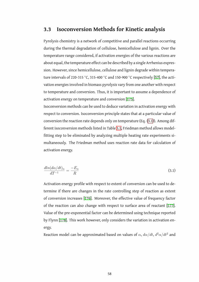
3.3 Isoconversion Methods for Kinetic analysis

Pyrolysis chemistry is a network of competitive and parallel reactions occurring

during the thermal degradation of cellulose, hemicellulose and lignin. Over the

temperature range considered, if activation energies of the various reactions are

about equal, the temperature effect can be described by a single Arrhenius expres-

sion. However, since hemicellulose, cellulose and lignin degrade within tempera-

ture intervals of 220-315 ◦C, 315-400 ◦C and 150-900 ◦C respectively [57], the acti-

vation energies involved in biomass pyrolysis vary from one another with respect

to temperature and conversion. Thus, it is important to assume a dependence of

activation energy on temperature and conversion [175].

Isoconversion methods can be used to deduce variation in activation energy with

respect to conversion. Isoconversion principle states that at a particular value of

conversion the reaction rate depends only on temperature (Eq. (3.1)). Among dif-

ferent isoconversionmethods listed in Table 3.1, Friedmanmethod allows model-

fitting step to be eliminated by analyzing multiple heating rate experiments si-

multaneously. The Friedman method uses reaction rate data for calculation of

activation energy.

dln(dα/dt)α

dT −1 = −Eα

R(3.1)

Activation energy profile with respect to extent of conversion can be used to de-

termine if there are changes in the rate controlling step of reaction as extent

of conversion increases [176]. Moreover, the effective value of frequency factor

of the reaction can also change with respect to surface area of reactant [177].

Value of the pre-exponential factor can be determined using technique reported

by Flynn [178]. This work however, only considers the variation in activation en-

ergy.

Reaction model can be approximated based on values of α, dα/dt, d2α/dt2 and

58

Table 3.1: Isoconversion or Model Free methods for kinetic analysis of TGA curve

Model Equation

Friedman Model ln(β dα

dT

)= ln(k0f(α)) − E

RT

KAS Model ln(

βT 2

)= ln

(k0R

Eg(α)

)− E

RT

Miura Maki Method ln(

βT 2

)= ln

(k0RE

)+ 0.6045 − E

RT

FWO Method ln(β) = ln(

k0REg(α)

)− 5.331 − 1.052 E

RT

activation energy. Eq. (3.3) [179] can be derived from Eq. (3.2)

f(α) = β

(dα

dT

)α

[Aαexp

(−Eα

RTα

)]−1

(3.2)

f ′(α)f(α) = 1

dαdt

(d2α/dt2

dα/dt+ 2β

Tα

− β

Eα

dEα

dT

)(3.3)

Where, f ′(α) is the derivative with respect to α and Eα, and Tα are activation en-

ergy and temperature values respectively at a giveα. A reactionmodel for kinetic

analysis of the data is selected by comparing the right hand side of Eq. (3.3), calcu-

lated using experimental values, with model graphs of f ′(α)f(α) for different reaction

models. The reaction model is used to derive the corresponding DAEM equations

for α,dα/dt,d2α/dt2.

3.4 Distributed Activation Energy Model

The general rate expression, as a function of temperature (T) and conversion (α)

is given as Eq. (3.4)

dα

dt= f(T, α) (3.4)

The first assumption is that differential Eq. (3.4) can be expressed in variable sep-

arated form as,

dα

dt= f(T )f(α) (3.5)

59

Solid state reaction is assumed to follow Arrhenius dependence as for the range of

energies required to activate solid state reactions, Maxwell-Boltzmann equation

holds good [180, 181]. Further, as biomass is composed of cellulose, hemicellulose,

lignin, and mineral matter, at the molecular level local chemical composition is

different. Biomass is porous in nature and the pore structure undergoes changes

during pyrolysis. Hence, the energy barrier, even for a single step reaction or any

heat and/or mass transfer step, can be a collection of values depending on the

location of the reaction center in the solid reactant [182, 183]. Thus, representa-

tion of reaction energy barrier using a unique value is not appropriate, and DAEM

[117, 184] is suitable for describing kinetics of biomass pyrolysis.

3.4.1 Assumptions

Following assumptions were made for developing the three component DAEM

model,

• There are infinite ′i′ parallel reactions occurring simultaneously during decom-

position of solid, so that each point on the TGA/DTG curve is a combination of

these infinite parallel reactions.

• The reactions follow the Arrhenius law.

• Activation energy of each reactions is a random variable and thus, it is safe to

assume that the activation energies can be expressed by a continuous probabil-

ity distribution function.

• For one pseudo-component frequency factor for every parallel reaction is as-

sumed to be the same.

• Frequency factor is a function of temperature.

3.4.2 Mathematical model

Biomass is assumed to bemade up of volatile and non-volatilematter. The volatile

matter is assumed to consist of non-condensible and condensible matter formed

due to the depolymerization reactions of cellulose, hemicellulose and lignin only.

60

Extractive compounds in the biomass are not considered amongst volatiles. Dur-

ing pyrolysis process, biomass undergoes multiple parallel reactions simultane-

ously. Formation of volatiles from the biomass due to ith reaction is expressed as

Eq. (3.6)

d(Vi/V ∗i )

dt= Aiexp

(−Ei

RT

)(1 − Vi

V ∗i

)n

(3.6)

Here, Vi is the amount reacted in the i reaction and dVi is the amount of volatiles

released in time dt. Ei is the activation energy and Ai is the frequency factor for

the i reaction. It is further assumed that each i reaction can produce a maximum

V ∗i volatiles. The value of V ∗

i is calculated as Eq. (3.7)

V ∗i = Mdry − M∞ (3.7)

Where, Mdry and M∞ are the initial dry weight of biomass, and final weight of

residue obtained after the completion of pyrolysis reaction. The completion of

biomass pyrolysis is marked by no further change in the mass loss rate. The term

(Vi/V ∗i ) in Eq.(3.8) is the conversion, αi, for i reaction.

αi = Mdry − Mt

Mdry − M∞(3.8)

Mt, is the amount of biomass remaining at time, t during the pyrolysis reaction.

It should be noted that the formation of volatiles by the nth order reaction is an

assumption. The reaction rate can be accelerating, decelerating, or sigmoid type.

Different models capable of describing such reaction rates are given in Table 3.2.

Here, g(α) =∫

d(α)/f(α)

For the derivation of DAEMequations, thenth order reactionmodel is chosen. The

integral form of Eq. (3.6) is written as

Vi

V ∗i

= 1 −[1 − (1 − n)

∫ t

0Aiexp

(−Ei

RT

)dt

] 11−n

n 6= 1 (3.9)

Vi

V ∗i

= 1 − exp

[−∫ t

0Aiexp

(−Ei

RT

)dt

]n = 1 (3.10)

61

Table 3.2: Kinetic models used in the solid-state kinetics

Type of Reaction Reaction Model Code f(α) g(α)

Accelerating Power Law P4 4α34 α

14

Accelerating Power Law P3 3α23 α

13

Accelerating Power Law P2 2α12 α

12

Decelerating 1-D diffusion D1 1/2α−1 α2

Decelerating 2-D diffusion D2 [−ln(1 − α)]−1 (1 − α)ln(1 − α) + α

Decelerating 3-D diffusion D3 32(1 − α)

23 [1 − ln(1 − α)

13 ]−1 [1 − (1 − α)

13 ]2

Decelerating First Order F1 (1 − α) −ln(1 − α)Decelerating nth Order Fn (1 − α)n (n − 1)−1(1 − α)1−n

Sigmoid Avrami-Erofeev A4 4(1 − α)[−ln(1 − α)]34 [−ln(1 − α)]

14

Sigmoid Avrami-Erofeev A3 3(1 − α)[−ln(1 − α)]23 [−ln(1 − α)]

13

Sigmoid Avrami-Erofeev A2 2(1 − α)[−ln(1 − α)]12 [−ln(1 − α)]

12

Sigmoid Random scission DP 2√

α(1 −√

α) −ln(1 −√

α)

The complexity of lignocellulosic biomass is such that a continuous distribution

f(E)of activation energies is assumedwhere∫ (E+∆E)

E f(E)dE describes theprob-

ability for the i reaction with the reaction having an activation energy between

E and E + ∆E. The mass fraction of volatile material with activation energies

between E and E + ∆E, dV at a given time t is given in Eq. (3.11)

dV = dV ∗f(E)dE (3.11)

dV =∞∑

i=1Vi at time t (3.12)

V ∗ =∞∑

i=1V ∗

i potential volatile matter (3.13)

Now, V ∗i and Vi are replaced by V ∗ and dV , respectively. Then Eq. (3.9) and Eq.

(3.10) become,

dV = V ∗

1 −[1 − (1 − n)

∫ t

0Aexp

(−E

RT

)dt

] 11−n

f(E)dE n 6= 1 (3.14)

dV = V ∗

1 − exp

[−∫ t

0Aexp

(−E

RT

)dt

]f(E)dE n = 1

(3.15)

62

To determine the total amount of volatiles released at time t, Eq. (3.14) and Eq.

(3.15) are integrated between 0 to ∞ . The limits here represent the activation

energies for i reactions in the probability distribution function. The integration

of Eq. (3.14) and Eq. (3.15) is

α = 1 −∫ ∞

0

[1 − (1 − n)

∫ t

0Aexp

(−E

RT

)dt

] 11−n

f(E)dE n 6= 1 (3.16)

α = 1 −∫ ∞

0exp

[−∫ t

0Aexp

(−E

RT

)dt

]f(E)dE n = 1 (3.17)

Where, α is the overall degree of conversion. Since, the experiments are carried

out under non-isothermal conditions at temperatures linearly varying with time

from a starting temperature, T0. Under the linear heating program Eq. (3.16) and

Eq. (3.17) can be rewritten as Eq. (3.18) and Eq. (3.19),

α = 1 −∫ ∞

0

[1 − (1 − n)

∫ T

T0

A

βexp

(−E

RT

)dT

] 11−n

f(E)dE n 6= 1 (3.18)

α = 1 −∫ ∞

0exp

[−∫ T

T0

A

βexp

(−E

RT

)dT

]f(E)dE n = 1 (3.19)

To derive the model parameters using the differential data from experiments is

recommended. Thus, Eq. (3.18) and Eq. (3.19) need to be differentiated. The

differential forms are expressed as Eq. (3.20) and Eq. (3.21),

dα

dT=∫ ∞

0

A

βexp

(−E

RT

) [1 − (1 − n)

∫ T

T0

A

βexp

(−E

RT

)dT

] 11−n

f(E)dE n 6= 1

(3.20)

dα

dT=∫ ∞

0

A

βexp

[−E

RT−∫ T

T0

A

βexp

(−E

RT

)dT

]f(E)dE n = 1

(3.21)

63

Where β is the heating rate and βdα/dT = dα/dt. f(E) is the probability dis-

tribution function and standard continuous distribution functions can be used in

the equations. Here, Gaussian distribution function, Eq. (4.6), is used,

f(E) = 1σ

√2π

exp

(−(E − E0)2

2σ2

)(3.22)

f(E) = c

[1

σ1√

2πexp

(−(E − E0,1)2

2σ21

)]

+ (1 − c)[

1σ2

√2π

exp

(−(E − E0,2)2

2σ22

)](3.23)

Where, the c is the weight factor for a bimodal Gaussian distribution. The fre-

quency factor can also be a function of temperature as in Eq. (3.24) and can be

replaced in the Eq. (3.18) to Eq. (3.21).

A = A0Tm (3.24)

To solve equations Eq. (3.18) to Eq. (3.21) an approximation for the inner temper-

ature integral is used. The approximation is shown in Eq. (3.25),

∫ T

T0T mexp

(−E

RT

)dT =

RT m+2

Eexp

(−ERT

)(0.99954E + (0.58058 + 0.044967m)RT )

E + (2.54 + 0.94057m)RT

(3.25)

Eq. (3.25) is a good approximation and reduces the computation time substan-

tially. The outer integral can be solved directly using MATLAB.

Eq. (3.18) to Eq. (3.21) are used when the decomposition rate of biomass is ex-

pressed using one pseudo-component. However, it is possible to express the de-

composition or conversion rate using multiple pseudo-components. Eq. (3.26),

Eq. (3.27) and Eq. (3.28) can be used for a multi-component DAEM.

α =p∑

c=1wcαc (3.26)

64

dα

dT=

p∑c=1

wcdαc

dT(3.27)

d2α

dT 2 =p∑

c=1wc

d2αc

dT 2 (3.28)

Where, wc, the pseudo-component fraction can be one of the parameters for op-

timization.

Eq. (3.32) is the objective function used for optimizing the DAEM parameters. The

objective function is the average of square root ofmean squared error forα, dα/dt

and d2α/dt2 curves.

J1 =√√√√ n∑

j=1

m∑i=1

(αexpt,ij − αpred,ij)2

n(3.29)

J2 =√√√√ n∑

j=1

m∑i=1

((dα/dt)expt,ij − (dα/dt)pred,ij)2

y2j n

(3.30)

J3 =√√√√ n∑

j=1

m∑i=1

((d2α/dt2)expt,ij − (d2α/dt2)pred,ij)2

z2j n

(3.31)

J = J1 + J2 + J3

3 (3.32)

Where n is the number of heating rates used simultaneously to fit the kinetic pa-

rameters, m is the number of points on each evaluated curve, y and z are the peak

maximum for each DTG and differentiated DTG curve. The use of y and z is to

normalize the objective function.

3.4.3 DAEM equations used for parameter optimization

The DAEM equations for α, dα/dt and d2α/dt2 using the three reaction models,

namely, first order equation (F1, Eq. (3.34) to Eq. (3.36)), Avrami-Eroofev (A2, Eq.

(3.37) to Eq. (3.39)) and random scission model (DP, Eq. (3.40) to Eq. (3.42)) have

65

been used for determining the apparent kinetic parameters. To avoid confusion

substitution in Eq. (3.33) is used in the DAEM equations derived for all reaction

models

I = A0

βT mexp

(−E

RT

)(3.33)

DAEM equations for first order reaction model,

α = 1 −∫ ∞

0exp

[−∫ T

T0IdT

]f(E)dE (3.34)

dα

dt= β

∫ ∞

0

A0

βT mexp

[−E

RT−∫ T

T0IdT

]f(E)dE (3.35)

d2α

dt2 = β2∫ ∞

0

A0

βT mexp

[−E

RT−∫ T

T0IdT

](−E

RT 2 − I + m

T

)f(E)dE (3.36)

DAEM equations for Avrami-Erofeev reaction model,

α = 1 −∫ ∞

0exp

[−(

12

∫ T

T0IdT

)2]f(E)dE (3.37)

dα

dt= β

∫ ∞

0

12

A0

βT mexp

[−(

12

∫ T

T0IdT

)2

− E

RT

][ ∫ T

T0IdT

]f(E)dE (3.38)

d2α

dt2 = β2∫ ∞

0

12

A0

βT mexp

[−(

12

∫ T

T0IdT

)2

− E

RT

][I +

(∫ T

T0IdT

)(m

T− 1

2I

(∫ T

T0IdT

)+ E

RT 2

)]f(E)dE (3.39)

DAEM equations for random scission model,

α = 1 −∫ ∞

0exp

[−(∫ T

T0

A0

βT mexp

(−E

RT

)dT

)2]f(E)dE (3.40)

66

dα

dt= β

∫ ∞

02[1 − exp

(−∫ T

T0IdT

)]exp

(−∫ T

T0IdT

)If(E)dE (3.41)

d2α

dt2 = β2∫ ∞

02Iexp

(−∫ T

T0IdT

)[(1 − exp

(−∫ T

T0IdT

))(

m

T+ E

RT 2

)+ I

(2exp

(−∫ T

T0IdT

)− 1

)]f(E)dE (3.42)

3.5 Materials and methods

3.5.1 Biomass Analysis

Mixture of wood and bark (mallee, species: E. polybractea) from the state ofWest-

ern Australia, Australia was used for pyrolysis reactions. Biomass was sieved into

different particle sizes and dried at 70◦C in a vacuum oven for 12 hours. The parti-

cle size distribution of sieved biomass particles was determined using theMalvern

Mastersizer 2000, LASER diffraction apparatus. An elemental analyzer (Thermo-

Scientific)was used to determine the elemental composition of biomass after siev-

ing. Further, the ash content of biomasswas also evaluated for all the particle sizes

considered in the study. Scanning electron microscope (Zeiss Neon 40EsB cross-

beam FESEM and, TESCAN MIRA3 VP-FESEM) was used to study the biomass and

the biochar surface morphology.

3.5.2 TGA Calibration

TGA used in this study (TGA-series 8000 from Perkin Elmer) was calibrated using

four different Curie point temperatures. The experimental temperature range

was between 150 to 700 ◦C, thus, alumel, nickel, perkalloy and iron were used as

reference materials because their Curie point temperature are 154.2, 355.3, 596

and 770 ◦C respectively. Small pieces, 2-3 mm in length, of each material were

used for the temperature calibration at experimental heating rates. Amagnet was

placed around the glass tube, surrounding the TGA furnace, which pulled the sam-

ple pan downwards. The downward pull caused an increase in weight of the pan.

As each material reached its Curie point temperature, loss in magnetic property

67

was recorded as weight loss on the TGA curve. The onset of Curie point temper-

ature for each material was calculated at different heating rates. As the heating

rate increased, the apparent Curie point temperature also increased. A graph of

apparent Curie point temperature vs. heating rate was plotted for each material.

Table 3.3 shows the parameters for linear calibration equation used for different

materials.

Table 3.3: TGA temperature calibration parameters valid for heating rates of 5-250◦C/min

Parameters Alumel Nickel Perkalloy Iron

slope 0.2683 0.1494 0.0867 0.0608intercept 163.16 361.95 588.85 774.73

R2 0.9936 0.9965 0.9957 0.9965

3.5.3 Thermogravimetric analysis of biomass

The particle sizes used in the literature for high heating rates is < 50 µm to ensure

uniform temperature throughout the particle. However, pore structure of such a

small particle size is not representative of biomass particles (order of 1 mm) used

in large scale pyrolysis reactors. Plasticity of biomass particles during pyrolysis

process can alter their pore structure and affect the volatile evolution rate. Par-

ticle sizes in the range of 0.1 to 0.4 mm are representative of biomass pore struc-

ture but may suffer from internal temperature gradients for high external heat

transfer coefficients as experienced in micropyrolyzers (Fig. 2.6). This is another

reason for the use of TGA apparatus and intermediate heating rates in this thesis,

which ensures isothermal conditions for particle sizes between 0.1 to 0.4 mm.

TGA was equipped with a chromel-alumel thermocouple at center of the TGA-

furnace (Figure 3.1). The thermocouplewas at a distance of 1 to 2mmfrombottom

surface of sample pan. Temperature recorded by the thermocouple was denoted

as the sample temperature in the instrument. Further, the ability of the equip-

ment to record the sample temperature and mass loss with an accuracy of 0.1 µg

and at a frequency of 8 Hz facilitated numerical differentiation of the TGA data

that generated the differential thermogravimetric (DTG) curve. Biomass with dif-

ferent particle sizes -≤45µm, 75 to 106 and 300 to 425 µmwas accurately weighed

68

in alumina pans. Typical weight of the sample taken for each experiment was a

function of heating rate of the TGA program. The sample weight was varied from

0.25 to 3.5mg for analysing the thermal lag under different heating rates. Biomass

pyrolysis was carried out under a argon flow rate of 60 ml/min at different linear

heating rates. Argon was used as a sweeping gas to carry the pyrolysis vapors out

of the furnace as soon as they were formed to suppress secondary pyrolysis reac-

tions. Each experiment was performed atleast three times. Table 3.4 shows the

temperature program for biomass pyrolysis.

Table 3.4: Non-isothermal TGA program for biomass pyrolysis

Step No.Initial Temperature

(◦C)Final Temperature

(◦C) Holding Time/Heating Rate

1 35 100 25◦C/min2 100 100 15 min3 100 150 25◦C/min4 150 150 15 min

5 150 7005/25/50/75/

150/200/250 ◦C/min6 700 700 20 min

Figure 3.1: Schematic representation of TGA8000 furnace and furnace tube. 1.Furnace, 2. Alumina pan, 3. Thermocouple, 4. Furnace glass tube, 5. Coolingjacket for furnace tube. All dimensions are in mm

69

3.5.4 Calculation of DTG curve

The raw data from TGA was normalized to α, which represented the extent of

volatiles released during biomass pyrolysis (Eq. (3.8)). The TGA data was nmer-

ically differentiated to yield a DTG curve. To reduce the noise in the DTG curve

equally spaced normalized TGA data was processed using the Soviztky-Golay dig-

ital filter (SG-filter) and filtered data was numerically differentiated, over a time

step of 0.5 seconds, using extended numerical differentiation [185].

3.5.5 Optimization of DAEM parameters

As lignocellulosic biomass comprises of cellulose, hemicellulose and lignin, the

biomass pyrolysis reaction was assumed to be a linear combination of degrada-

tion of the three pseudo-components. Gaussian distribution function was used to

model the activation energy distribution for each component. Activation energy

distribution of one of the pseudo-component was further assumed to follow a bi-

modal distribution, describing two distinct set of reactions [119]. Optimization of

DAEM parameters was carried out using fmincon solver in MATLAB. The gradient

of objective function with respect to each parameter was specified to accelerate

the convergence of the solver and stabilize the solution. The square root of mean

squared error for α, dα/dt and d2α/dt2 curves was simultaneously minimized to

reduce the number of solutions obtained from optimization of a 16-parameter

equation.

3.6 Results and Discussion

3.6.1 Biomass Analysis

Post sieving particle size analysis of biomass is shown in Table 3.5. Biomass par-

ticles were not spherical but needle like. Volume weighted mean diameter of the

particles obtained from light scattering experiment was representative of longer

dimension of the biomass particle. On the other hand, shorter dimension of the

biomass particle was in the range of the sieve used for size-based separation. Op-

tical microscope images (not shown) and mean value in Table 3.5 led to the con-

70

clusion that for biomass particles≤45 µm the aspect ratio was close to one.

Table 3.5: Particle Size Distribution of biomass. D(v,0.1), D(v,0.5) and D(v,0.9) is theparticle size below which 10, 50 and 90 vol.% of the sample lies

BiomassSieveSize Range (µm)

VolumeWeightedMean (µm)

D(v,0.1)(µm)

D(v,0.5)(µm)

D(v,0.9)(µm)

Span

≤45 42.09±0.04 17.53±0.13 38.35±0.04 72.45±0.03 1.43±0.0175 to 106 151.59±2.05 58.35±0.30 120.84±0.45 252.11±2.49 1.61±0.02300 to 425 706.17±15.32 275.19±1.73 632.46±5.69 1284.28±13.76 1.59±0.01

Biot number for the particles was calculated using two different characteristic

lengths for the three particle sizes. One characteristic length usedwas the volume

weightedmeandiameter and the other valuewas the longest dimensionunder the

column D(v,0.9) from Table 3.5. For particle size, between 300 to 425 µm, Figure

3.2 shows that the Biot number exceeds one when the heat transfer coefficient

in greater than or equal to 100. Biot number for other two particle sizes is below

one for all values of heat transfer coefficients. The carrier gas flow rate used in

the TGA program was 60 ml/min, which made the flow inside the furnace tube

laminar. The magnitude of heat transfer coefficient for the annular region with

characteristic length of 0.5 cm and thermally developing flow was of the order of

10 W/mK. Therefore, it was safe to assume that Biot number for all the particle

sizes is less than 1. Thus, the heating rate of particle was assumed to be the same

as TGA program.

3.6.1.1 Elemental and Ash content of biomass

Biomass is a heterogeneous material composed of three bio-polymers and several

minerals like calcium, potassium, sodium, silica, iron, and aluminum [186]. In the

current study biomass considered for the experiment was a mixture of wood and

bark. Table 3.6 shows results of elemental and ash content analysis of biomass

with respect to different particle sizes. The elemental composition of biomass did

not vary significantlywith the particle size. The variation in the ash content could

be linked to the difference in the grinding characteristics of wood and bark. Bark

is more brittle than wood and can be ground to finer particle size as compared to

wood. The elemental and ash content of Mallee wood and bark was in the range

71

(a)

(b)

Figure 3.2: Biot number for two characteristic lengths for three particle sizes inTable 3.5 (a) 42.088, 151.588, 706.165 µmand (b) 72.449, 252.114, 1284.282 µm. Thethermal conductivity of biomass is assumed to be 0.105 W/mK [21]

72

as reported by Abdullah et al. [187, 188]. Biomass particle size ≤45 µm was rich

in ash, whichmight be indicative of higher bark content when compared to other

particle sizes.

Table 3.6: Elemental analysis and ash content of biomass. ∗Oxygen content wascalculated by difference.

BiomassParticleSize (µm)

C H N O∗ Ash

≤45 44.67±0.15 4.99±0.53 0.21±0.01 50.13±0.50 6.24±0.3075 to 106 46.62±0.12 5.96±0.31 0.18±0.01 47.24±0.38 1.24±0.42300 to 425 45.82±0.14 5.83±0.46 0.13±0.01 48.22±0.43 1.37±0.25

3.6.2 Thermogravimetric analysis of biomass

3.6.2.1 Effect of initial sample weight

Large sample weight and high heating rates can lead to thermal lag in the sam-

ples due to the endothermic nature of pyrolysis reaction [78]. As the heating rate

increases the effect of initial sample weight becomes prominent as shown in Fig-

ure 3.3. For heating rates upto 75◦C/min, there is no shift in the TGA profile of

biomass pyrolysis in terms on initial sample weight. However, for heating rate

of 150◦C/min and above the TGA curve shifts to high temperatures as the sample

weight is reduced from 3.5 to 0.25mg. Therefore, initial sample weight chosen for

heating rates between 5 and 75◦C/min and, 150 and 250 ◦C/min was 3.5 and 0.5

mg respectively.

3.6.2.2 Processing of TGA and DTG curve for pyrolysis kinetics

The SG-filter is a good choice for data smoothing because it does not cause the

curve to shift with respect to temperature or time [185]. The processed DTG curve

shows that the peakmaximum, peak resolution and peak position was not altered

due to smoothing (Figure 3.4).

73

3.6.2.3 Effect of heating rate and biomass particle size on TGA profile

The TGA and DTG profiles of biomass pyrolysis with respect to heating rate and

particle size are shown in Figure 3.5. In this study, ash content of biomass varied

with the particle size. Therefore, the organic content of final residue obtained at

different heating rates was compared with respect to the particle size.

The total solid residue values in Table 3.7 suggest that there was no significant

(a)

(b)

The figure is continued on the next page...

74

(c)

Figure 3.3: Effect of weight on the biomass pyrolysis TGA profile for heating rate(a) 5 ◦C/min (b) 75 ◦C/min (c) 250 ◦C/min

difference between the organic content of solid residue obtained after comple-

tion of pyrolysis for heating rates upto 75 ◦C/min. The TGA temperature program

has an isothermal step, where the biomass was held for 20 min at 700 ◦C. Table

3.7 and Table 3.8 indicate that mass was also lost in the isothermal region of TGA

program. Difference between organic residue for particle size ≤45µm and other

two sizes is a consequence of char forming reactions catalyzed by higher mineral

content in biomass≤45µm [186]. On the other hand, a significant change in solid

residue was observed for particle size 75 to 106 and 300 to 425 µm, and heating

rate of 200 and 250 ◦C/min. Increase in heating rate increases the selectivity for

depolymerization, which causes a decrease in the solid residue. Moreover, high

heating rates bring about significant change in morphology of the particles lead-

ing to the formation of open pore structure which facilitates the volatiles release.

On the other hand small particles, here particles with≤45µm, can sinter and lead

to increased resistance for volatilization. Thus, the solid residue for particle size

between 75 to 106 and 300 to 425 µm, where ash content is less and particles are

spread apart from one another, have lower organic char as compared to particles

with size≤45 µm.

75

(a)

(b)

Figure 3.4: (a) Unprocessed TGA and DTG curves (b) TGA and DTG curves afterapplying Sovitzky-Golay filter

The percent of biomass reacted at temperatures shown in Table 3.8 represents the

data recorded during pyrolysis of biomass heated at different heating rates to a

final temperature of 700 0C . In temperature range of 400 to 600 ◦C, for biomass

with particle size ≤45 µm, the amount of biomass reacted was less as compared

76

(a)

(b)

This figure is continued on the next page...

Figure 3.5

77

(c)

(d)

This figure is continued on the next page...

Figure 3.5

78

(e)

(f)

Figure 3.5: Processed (a) to (c) TGA curves and (d) to (f) DTG curves for threebiomass particle sizes and heating rate varying from 5 to 250 ◦C/min.

79

Table 3.7: Solid Residue left after pyrolysis of biomass, with different particle size,under pre-defined linear heating rate programs. Values in parenthesis are ob-tained after subtracting the ash content from the solid residue.

Heating Rate(◦C/min)

Final Solid Residue(wt.% of dry biomass)

<45 µm 75 to 106 µm 300 to 425 µm

525.04±0.20(18.80)

20.86±0.41(19.62)

18.29±0.03(16.42)

2524.99±0.19(18.74)

20.62±0.15(19.38)

18.80±0.39(16.93)

5024.67±0.06(18.43)

20.54±0.26(19.30)

18.86±0.03(16.98)

7525.11±0.06(18.87)

19.46±1.90(18.21)

18.21±0.54(16.34)

15023.26±0.78(17.02)

20.09±0.15(18.85)

18.42±0.28(16.55)

20024.65±0.05(18.41)

12.45±0.24(11.21)

10.23±0.97(8.86)

25021.65±0.68(15.41)

12.78±1.01(11.54)

8.82±0.16(7.45)

to other two particle sizes. This is because the high mineral content in biomass

particles≤45 µmpromotes char forming reactions [189, 190]. As the heating rate

increases, the extent of mass reacted decreases because the time spent by the

biomass particle in any small temperature interval decreases. On the other hand,

between 300 and 600 ◦C, the percentage of biomass reacted increases beyond 150◦C/min for all particle sizes (Table 3.8). The increase in the mass loss might a

consequence of increase in selectivity for devolatilization reactions that facilil-

tates formation of porous structure, which in turn allows easy passage of volatile

products out of the biomass particle. It is important to note that for 5 ◦C/min the

percent biomass reacted up till 300 and 400 ◦C was much higher than any other

heating rate because the reaction time was 30 min. The evolved gases were not

analyzed and therefore, it was not possible to comment if the gas evolved at 300◦C under 5◦C/min heating had the same chemical composition as those evolved

for other heating rates.

To get a better insight into effect of pyrolysis conditions on biomass particle, op-

tical microscope and SEM images of intermediate and final solid residue were an-

alyzed. The pore structure of biomass used in this study was visualized using SEM

80

images. The lumen diameter of the biomass was between 4 to 10 µm while the

diameter of the vessel cells was of the order of 20 to 40 µm. Further the vessel

cells had small pores on their wall ( 0.5 to 1.5 µm), implying that there was some

degree of open pore structure already present in biomass particle. Ciesielski et al.

[53] imaged pinewood particles using confocal scanning lasermicroscopy and the

cell wall thickness was of the order of 2 to 4µmand the lumen diameter was of the

order of 101 µm. Biomass particles, 300 to 425 µm, in Figure 3.6 revealed that the

cell wall structure of the biomass was retained at an intermediate temperature of

300 ◦C and at all heating rates used in the study [34, 191].

81

Table3.8:PercentM

assReactedwithrespecttotemperatureatdifferentheatingratesfordifferentparticlesizes

MassReacted(wt.%

ofinitialdrybiomass)

300

◦ C400

◦ C500

◦ C600

◦ CHeatingrate

◦ C/min

<45

µm

75to106

µm

300to425

µm

<45

µm

75to106

µm

300to425

µm

<45

µm

75to106

µm

300to425

µm

<45

µm

75to106

µm

300to425

µm

527.78

28.56

27.25

60.50

68.05

71.99

65.75

72.92

76.43

69.10

75.72

78.89

2520.19

21.13

20.73

58.58

66.55

70.70

64.69

72.51

76.03

68.11

75.55

78.64

5018.04

18.78

18.75

57.60

63.95

69.89

64.87

71.85

75.61

68.43

74.84

78.26

7516.22

17.21

18.61

55.26

61.91

69.70

64.04

71.00

75.48

67.89

74.06

78.11

150

17.73

16.22

14.07

55.61

59.51

60.32

65.99

72.07

74.74

69.56

75.29

77.79

200

17.67

19.24

14.87

54.61

63.44

63.29

64.37

75.27

78.07

68.15

77.97

80.32

250

18.14

20.21

19.47

56.58

63.71

68.80

68.41

77.56

81.68

72.09

80.13

83.16

82

The preservation of the cell wall structure during pyrolysis suggested that the

biomass maintains its macro-porosity even under pyrolysis conditions. This im-

plied that the intra-particle mass transfer resistance for the pyrolysis vapors to

escape from the particle was low. For a particle with a length of 700 µmand a pore

size of the order of 5 to 10 µm, the characteristic time for vapor diffusion along

the length of the particle was of the order of 0.50 sec, when the effective diffusion

coefficient was assumed to be 10−6 m2/s [100]. However, the vapor would not al-

ways travel along the length of the particle it could also travel radially as a result

of formation of pores on the cell wall of biomass during pyrolysis.

Figure 3.6: SEM images of (A1, A2) Biomass (300 to 425µm); (A3) Biomass (≤45µm);intermediate biochar obtained for biomass particle size of 300 to 425 µm at 300 ◦Cunder heating rates of (B1) 5 ◦C/min, (B2, B3) 25 ◦C/min, (B4) 75 ◦C/min, (B5) 150◦C/min and (B6) 250 ◦C/min

The pores formed on the cell wall because volatiles evolved as a consequence of

bubble eruption [76, 71]. Biomass particle passed through an intermediate vis-

83

coelastic phase and pyrolysis vapors nucleated in the form of bubbles inside the

partially molten phase. Melting could occur as a result of thermal lag [192] or

partial depolymerization [78] at moderate heating rates, where the depolymer-

ized product might condense immediately inside or on the surface of the particle.

The particle sizes considered in this study do not experience considerable thermal

lag ([53] and Figure 3.2). Therefore, biomass surface melting could be explained

by partial depolymerization that generated non-volatile and volatile oligomers.

The high resolution SEM images in Figure 3.7 (A1) to (A4), where the cell wall was

in focus, showed the presence of bubbles (length scale 101 nm) on surface [53]. As

the heating rate increased, the mean diameter of the bubble decreased while the

number density of bubbles increased. This was in accordance with the nucleation

phenomenon, where slow heating rates allow nuclei growth, which subsequently

erupted as large bubbles to release the volatiles. The bubbles in the cell wall expe-

rience overpressure at high heating rate which caused formation of a open struc-

tured solid as compared to unreacted biomass [79]. Therefore, beyond a certain

heating rate, 150 ◦C/min in this case, the amount of volatiles released increased

at 300 and 400 ◦C despite decreasing reaction time (Table 3.8).

Figures 3.7 (A5) and (A7) show bubble features, with a diameter of the order of 20

to 40 µm, that formed on outer surface of the biomass particle when the heating

rate of TGA program was greater than or equal to 75◦C/min. This might be due

to large amount of vapor accumulated inside biomass particle having a viscous

liquid boundary at the surface. Formation of large bubbles could hinder the re-

lease of vapors. Optical microscope image in Figure 3.7 (A7) revealed that bubble

features, marked from 1 to 4, were preserved even after holding the biochar at

700 ◦C for 20 min, indicative of cross-linking reactions which increased the me-

chanical strength of the bubble boundary. However, some bubbles might erupt at

high temperatures, which could explain the increase in the height of the second

peak in DTG curves for biomass particle size of 75 to 106 and 300 to 425 µm (Fig-

ure 3.5 (d) to (f)). The vapor trapped inside the bubbles might not be originating

only from particle surface but might be coming from inside the particle. If this

was true, the large bubbles may result in formation of open pore structure. This

could serve as an alternative explanation for the data representing an increase in

84

biomass conversion beyond 150 ◦C/min presented in Table 3.8. Further, though

large bubbles were not observed when the initial biomass particle size in≤45 µm,

the formation of loosely bound agglomerate above 150 ◦C/min, shown in Figure

3.7 (A8) also demonstrated presence of intermediate molten phase during pyrol-

ysis. Shrinkage also appears to occurred from the edges of the agglomerate as a

whole.

Figure 3.7: SEM images of biochar obtained at the end of TGA program with heat-ing rate (A1) 25 ◦C/min, (A2) 75 ◦C/min, (A3) 150 ◦C/min, (A4) 250 ◦C/min; in-termediate biochar obtained for biomass particle size of 300 to 425 µm at 300 ◦Cunder heating rates of (A5) 75 ◦C/min, (A6) 250 ◦C/min; optical microscope imagefor biochar obtained at the end of TGA program with heating rate of 150 ◦C/minfor biomass particle size of (A7) 300 to 425 µm and (A8)≤45µm

Optical microscope images (Figure 3.8) also revealed particle shrinkage along the

smaller dimension of the particles. Image analysis of particles (300 to 425 µm)

showed that the average external surface area (average of 82 particles) of unre-

85

acted biomass particles was 0.622 ± 0.236 mm2. The average external surface of

solid particles obtained under 5 ◦C/min and 250 ◦C/min was 0.364 ± 0.156 mm2

(averaged over 48 particles) and 0.442 ± 0.136 mm2 (averaged over 32 particles)

respectively. The percent reduction in area due to shrinkage, based on initial ex-

ternal surface area, for particles obtained at 5 and 250 ◦C/min was 41.48 % and

29.01 % respectively. Despite same final conversion value, the reduction in the

external surface area of 300 to 425 µm biomass particle at high heating rate was

less because of possible pyrolysis product accumulation within the particle.

The foregoing discussion indicates that, morphological changes during decom-

position would not lead to a constant shift in all measurement temperatures of

the TGA and DTG curves with respect to the heating rate [78]. The morphological

changes affect volatilization rate and hence, affect the value of DAEM parameters.

Also, as large bubbles were observed beyond 300 ◦C, a good approach for simu-

lating DTG curves would be considering temperature dependence of frequency

factor in the kinetic expression (A=A0Tm). Further, the choice of TGA data gen-

erated at different heating rates for obtaining the DAEM parameters would affect

the predictability of TGA curves for heating rates outside the range considered in

this study.

(a)

The figure is continued on the next page...

Figure 3.8

86

(b)

(c)

Figure 3.8: Optical microscope images of particles before and after pyrolysis (a)Biomass, 300 to 425 µm, (b) Biochar obtained at 5 ◦C/min, (c) Biochar obtained at250 ◦C/min.

3.6.3 TGA data analysis using isoconversion method

Among different isoconversion methods, the most widely used method is Fried-

man method (Table 3.1). The Friedman method uses instantaneous reaction rate

values for determination of activation energy, and frequency factor. The advan-

tage of themethod is that it does not require an assumption of any reactionmodel.

87

The profile of apparent activation energy (Figure 3.9) with respect to conversion

offers some insight into probablemechanism of the reaction [176]. For all the par-

ticle sizes considered in this work, qualitative and quantitative profiles of activa-

tion energy with respect to extent of conversion were not significantly different.

88

(a)

(b)

This figure is continued on the next page...

Figure 3.9

The activation energy increases linearly up toα=0.3 and thendecreases in a slightly

concave manner from α=0.3 up to α=0.7. Beyond α=0.7 the activation energy in-

89

(c)

Figure 3.9: Isoconversion method plots for three particle sizes. Variation of acti-vation energy with respect to extent of reaction.

creases again which corresponds to the presence of competitive parallel reactions

[176]. Afterα=0.3 there is a transition or a change in the rate limiting step and the

slight concave decrease of the activation energy may indicate reversible reaction

[176]. On the other hand, the profile of frequency factor (Figure 3.10) versus acti-

vation energy shows kinetic compensation effect, which indicates that theremust

be multiple chemical changes originating from similar chemical structure or due

to differences arising due to heat and mass transfer limitations [193]. As the heat

transfer coefficient is of the order of 10W/mK, Biot number of all the biomass par-

ticles was assumed to be less than 1. Therefore, the linear decrease of ln(A) from

α=0.3 to α=0.7 implied that there are iso-kinetic reactions/processes occurring in

these regimes. This also suggested that different reactions/processes occurred

over similar time scale and were thus, difficult to decouple.

Furthermore, the obtained profile of activation energy was used to determine the

reactionmodel using Eq. 3.3 in section 3.3. The plots for different reactionmodels

in Table 3.2 are shown in Figure 3.11 ((d) to (f)). Experimental values of the left

hand side of Eq. 3.3 compared well qualitatively with all the Avrami-Erofeevmod-

90

els, and the random scission model. Reaction models DP and A2 were selected for

fitting the DAEM parameters to biomass pyrolysis. The random scission model

used here assumes that products that have a degree of polymerization greater

than two are non-volatile [174]. The assumption enables analytical integration of

f(α), which is required to derive the DAEM equations for random scission model.

Moreover, microscopic evidence of molten phase and bubble nucleation on the

biomass surface justify the approximation of DP and A2 reaction models. First

order reaction model is widely used for determining the kinetic parameters of

biomass devolatilization. Therefore, DAEMparameters were also obtained assum-

ing first order (F1) reaction model.

3.6.4 DAEM kinetic parameters

The DAEM parameter optimization was carried out considering different cases

mentioned in Table 3.9. The effect of reaction model, and TGA, DTG, and differ-

entiated DTG curves corresponding to different set of heating rates on DAEM pa-

rameters was considered in the study.

Table 3.9: Details for different cases used for DAEM parameter optimization.

Case no.Heating rates used for DAEM

parameter optimization (◦C/min)

Reaction Model: F1

Case 1 5 to 250Case 1A 5 to 75Case 1B 150 to 250

Reaction Model: DP

Case 2 5 to 250Case 2A 5 to 75Case 2B 150 to 250

Reaction Model: A2

Case 3 5 to 250Case 3A 5 to 75Case 3B 150 to 250

3.6.4.1 Number of pseudo-components

Presence of two peaks in the DTG curve implies at least two pseudo components

be used formodel fitting exercise [118, 119]. Three pseudo-componentswere used

91

(a)

(b)

This figure is continued on the next page...

Figure 3.10

92

(c)

(d)

This figure is continued on the next page...

Figure 3.10

93

(e)

(f)

Figure 3.10: (a) to (c) Isoconversion method plots for three particle sizes. Varia-tion of Frequency factor with respect to activation energy. (d) to (f) Isoconversionmethod plots for three particle sizes. Linearity plots for ln(d(α)/dt) vs. (1/T)

94

(a)

(b)

This figure is continued on the next page...

Figure 3.11

95

(c)

(d)

This figure is continued on the next page...

Figure 3.11

96

(e)

(f)

Figure 3.11: (a to c) Comparison of experimental and Model reaction plots for Eq.3.3. (d to f) Model reaction plots for different reaction models for Eq. 3.3

97

to model the TGA, and DTG characteristics of the biomass under different pyroly-

sis conditions. The frequency factors of each pseudo-component was considered

to be constant. Hemicellulose undergoes two different set of reactions [119] and

hence, for the third pseudo-component single frequency factor, and a bimodal

Gaussian distribution were used to represent the kinetic characteristics .

3.6.4.2 Choice of objective function

To justify the choice of objective function used in this study DAEM parameters

were calculated using three different objective functions. In the first case only α

values were used for evaluating DAEM parameters, that is, only J1 (Eq. (3.29)) was

used as an objective function. In the second case average of J1 (Eq. (3.29)) and J2

(Eq. (3.30)) and in the third case average of J1 (Eq. (3.29)), J2 (Eq. (3.30)) and J3

(Eq. (3.31)) were used. The parameters were obtained by minimizing the objec-

tive function for all three cases using heating rates varying from 5 to 75 ◦C/min.

Initial guess value for the parameters was kept constant for all three cases. Rep-

resentative plots of experimental and predicted curves are shown in Figure 3.12.

It is evident from Figure 3.12 that only using J1 as an objective function is not a

good choice because the prediction for differential and double differential curves

is poor as compared to second and third case. Moreover, DAEM equation in this

study is a 16 parameter equation, which has multiple solutions. One way to re-

duce the number of solutions is to simultaneously optimize DAEM parameters for

α, dα/dt and d2α/dt2.

98

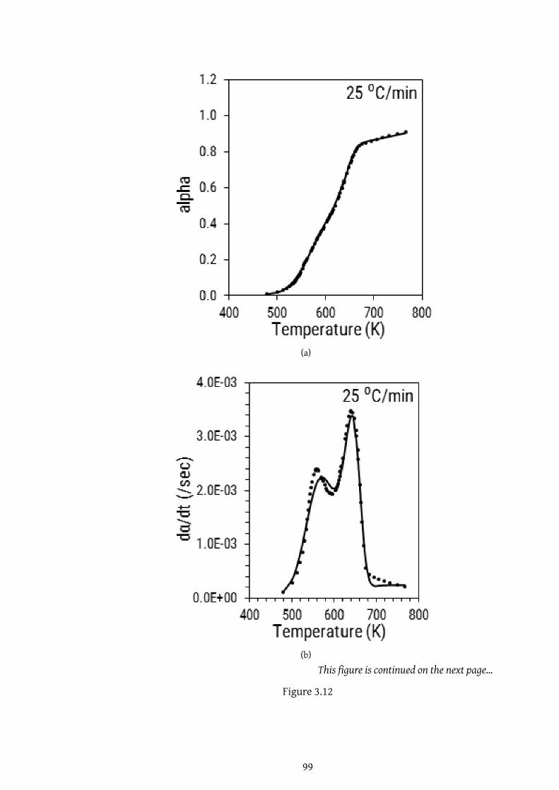
(a)

(b)

This figure is continued on the next page...

Figure 3.12

99

(c)

(d)

This figure is continued on the next page...

Figure 3.12

100

(e)

(f)

This figure is continued on the next page...

Figure 3.12

101

(g)

(h)

This figure is continued on the next page...

Figure 3.12

102

(i)

Figure 3.12: Comparison of experimental and predicted plots for α, dα/dt andd2α/dt2 using objective function in (a) to (c) case 1, (d) to (f) case 2, and (g) to (i)case 3

There is a significant difference between the value of m between option 2 and

option 3 as shown in Table 3.10. An average value of J1, J2 and J3 are used for

DAEM parameter optimization.

3.6.4.3 Effect of reaction model

The infinite reactions of each pseudo-component were assumed to follow either

a first order, random scission, or Avrami-Erofeev reaction model. To visualize the

effect of reaction model, plots of α vs time were compared at a constant temper-

ature of 673 K for same values of DAEM parameters (Figure 3.13). Three set of

parameters were used to compare the effect of reaction model. The parameters

in Table 3.11 were obtained by minimizing the objective function, J in Eq. (3.32)

for heating rates varying from 5 to 250 ◦C/min. The parameter calculation was

performed considering one reaction model at a time.

103

Table 3.10: Optimized DAEM parameters for a same initial guess value for Option1: J1 is objective function, Option 2: mean of J1 and J2 is objective function, Option3: mean of J1, J2 and J3 is objective function

Set no. wc2-Gaussian modelweight fractions

E0(kJ/mol)

σ(kJ/mol)

log(A0)(sec−1) m obj func

initial guess 0.2262 189.229 39.883 10.511 0.29430.2383 226.236 8.216 19.2830.5355 0.4473 163.038 7.110 11.857

0.5527 173.812 3.838

Option 1 0.2121 190.451 39.354 6.204 1.7732 J1=0.01140.4039 227.155 12.848 14.414 J2=0.05660.3840 0.0214 163.588 9.292 7.935 J3=1162

0.9786 179.569 2.178

Option 2 0.2195 189.871 38.988 7.403 1.4532 J1=0.01440.2123 226.270 8.227 15.617 J2=0.04280.5682 0.3208 163.165 9.300 8.876 J3=0.0843

0.6792 179.571 2.484

Option 3 0.2227 189.245 39.715 10.606 0.2876 J1=0.01780.2268 226.244 7.150 18.917 J2=0.04810.5505 0.3443 163.057 7.429 11.718 J3=0.0753

0.6557 174.681 0.996

Table 3.11: DAEM parameters derived using three different reaction models forpyrolysis of biomass having particle size ≤45 µm. Parameters in set number, (1)derived for DP, (2) derived for F1, (3) derived for A2

Set no. wc2-Gaussain modelweight fractions

E0(kJ/mol)

σ(kJ/mol)

log(A0)(sec−1) m obj func (J)

1 0.2768 180.139 3.582 13.062 0.0682 0.10370.3418 226.840 9.758 19.7760.3813 0.3317 153.219 3.075 11.643

0.6683 198.555 44.258

2 0.2441 189.278 40.289 10.158 0.2103 0.10680.2452 226.614 7.182 19.2970.5107 0.356 164.128 5.883 12.274

0.644 177.291 2.970

3 0.2105 171.258 20.200 8.736 0.1575 0.11270.2766 227.505 9.300 19.8770.5128 0.4784 161.544 7.445 12.333

0.5216 173.232 4.690

Differences between the conversion values are prominent only in Figure 3.13 (a),

while other two plots do not show considerable difference between the behavior

of different reaction models. However, it was not possible to determine a priori

which set of DAEM parameters would be insensitive to the reaction model used.

104

Therefore, all three reaction models were used to describe the volatilization be-

havior of biomass. The DAEM parameters calculated for reactionmodel, DP, were

selected amongst different configurations listed in Table 3.9 and tabulated in Ta-

ble 3.13.

Both random scission (DP) and Avrami-erofeev (A2) reaction models are used for

description of sigmoidal reaction rates. The DPmodel suggests that the polymers

in lignocellulosic biomass undergo homolytic scission and lead to formation of

two active species which further degrade until a point where volatile species are

formed. It may also involve end chain scission resulting in formation of volatile

species directly. On the other hand the A2 model assumes that reactions occur

at particular locations, called nuclei, in the solid. Nuclei are reactive sites in the

solid and their number density depends on temperature. Thus, as the heating rate

increases nuclei number density increases. These nuclei undergo different reac-

tions and result in the formation of volatile species. Molecular modelling studies

show that there is formation of active cellulose, hemicellulose, and lignin which

undergo degradation to volatile species and char. These active species can either

be oligomers or molecular intermediate. It is difficult to select the model based

on regression coefficient because all the reaction models have physical relevance

to pyrolysis reaction chemistry and have fairly close regression coefficients.

3.6.4.4 Effect of particle size and heating rate on DAEM parameters

The effect of heating rate and particle size on DAEM parameters is discussed to-

gether as the dependence on two varibales is interlinked with each other. The

three different particle sizes in this study take into consideration different scales

of intra-particle pore structure of biomass as discussed in section 3.6.2.3. Figure

3.14 shows the value of peakmaximum increases linearlywith the heating rate for

all particle sizes. The slope for each line is different, which can be attributed to

difference in composition of biomass particle size ≤45 µm and 75 to 106 and 300

to 425 µm. But, as the ash and elemental content of biomass with particle size 75

to 106 and 300 to 425 µm is quiet similar, the difference in the slope and high val-

ues of (dα/dt)max for 300 to 425 µm can be attributed to intra-particle secondary

reactions.

105

(a)

(b)

This figure is continued on the next page...

Figure 3.13

106

(c)

Figure 3.13: Conversion plots for three reaction models calculated using threedifferent set of DAEM parameters in Table 3.11, (a) For set no. 1, (b) For set no. 2,(c) For set no. 3.

Figure 3.14: Profile of (dα/dt)max with respect to heating rate for three particlesizes.

107

Table 3.12: Optimized DAEM parameters for three particle sizes for Case 1, 1A and1B

Particle size≤45 µm

Set no. wc2-Gaussain modelweight fractions

E0(kJ/mol) σ(kJ/mol)

log(A0)(sec−1) m obj func

Case 1 0.2441 189.278 40.289 10.158 0.2103 0.10680.2452 226.614 7.182 19.2970.5107 0.356 164.128 5.883 12.274

0.644 177.291 2.970

Case 1A 0.2704 189.200 40.318 10.131 0.1469 0.05050.2682 226.188 8.728 19.1950.4614 0.3316 162.347 6.881 12.092

0.6684 174.206 0.850

Case 1B 0.1724 190.157 37.616 3.915 2.0853 0.03940.2602 225.691 9.793 14.2920.5673 0.5509 166.397 10.592 7.344

0.4491 179.851 2.349

Particle size 75 to 106 µm

Case 1 0.1744 189.209 40.283 10.203 0.2509 0.13110.2539 226.323 7.737 19.2980.5717 0.3554 162.517 6.278 11.950

0.6446 174.773 2.689

Case 1A 0.2227 189.245 39.715 10.606 0.2876 0.04640.2268 226.244 7.150 18.9170.5505 0.3443 163.057 7.429 11.718

0.6557 174.681 0.996

Case 1B 0.1283 189.616 39.162 6.852 0.9859 0.04020.2655 226.308 8.631 17.4550.6062 0.4075 162.963 7.526 10.131

0.5925 175.007 2.211

Particle size 300 to 425 µm

Case 1 0.1700 189.538 39.151 8.732 1.3973 0.12730.1472 226.733 5.175 15.9990.6828 0.322 163.983 11.140 9.285

0.678 181.712 2.622

Case 1A 0.1309 189.660 39.508 6.520 0.7666 0.05190.2193 226.114 7.873 17.2520.6498 0.2204 162.343 10.008 11.020

0.7796 182.848 0.658

Case 1B 0.1090 189.956 38.744 3.775 2.0387 0.06520.1794 226.612 6.155 14.5090.7116 0.3372 162.324 6.643 7.476

0.6628 179.372 2.074

108

Table 3.13: Optimized DAEM parameters for three particle sizes for Case 2, 2A and2B

Particle Size≤45 µm

Set no. wc2-Gaussain modelweight fractions

E0(kJ/mol)

σ(kJ/mol)log(A0)(sec−1) m obj func

Case 2 0.2369 189.484 40.473 10.240 0.3006 0.10510.2952 227.277 8.929 19.3180.4679 0.3013 166.075 4.723 12.391

0.6987 179.388 4.590

Case 2A 0.2838 189.147 40.338 10.738 0.2288 0.05540.2682 226.274 9.380 19.2890.4481 0.4459 162.414 6.553 11.963

0.5541 173.925 2.694

Case 2B 0.1829 189.226 40.422 9.367 0.4013 0.02540.3563 225.777 10.826 19.0670.4608 0.5519 163.815 7.379 11.671

0.4481 173.031 3.205

Particle Size 75 to 106 µm

Case 2 0.1812 189.224 39.893 10.590 0.3620 0.13150.2685 226.250 8.839 19.2360.5503 0.4847 162.904 7.114 11.733

0.5153 174.229 3.651

Case 2A 0.1994 189.225 39.894 10.503 0.2774 0.05820.2547 226.236 8.427 19.2320.5459 0.4420 162.939 7.111 11.816

0.5580 173.991 2.878

Case 2B 0.1230 189.458 38.812 8.581 0.4460 0.04980.2988 226.274 9.613 19.1620.5782 0.5690 164.663 7.975 11.721

0.4310 174.267 3.153

Particle Size 300 to 425 µm

Case 2 0.1773 189.261 40.022 9.960 1.2237 0.13110.1693 226.614 6.019 16.7790.6534 0.3796 163.067 7.952 9.514

0.6204 176.808 3.900

Case 2A 0.2128 189.231 39.403 11.198 0.4679 0.05040.1362 227.130 5.745 18.7210.6510 0.4674 164.912 9.143 11.666

0.5326 179.116 1.603

Case 2B 0.1044 189.599 39.533 6.013 1.2344 0.03010.2493 226.280 7.956 16.8360.6463 0.4867 164.714 7.734 9.578

0.5133 175.866 2.756

109

Table 3.14: Optimized DAEM parameters for three particle sizes for Case 3, 3A and3B

Particle size≤45 µm

Set no. wc2-Gaussain modelweight fractions

E0(kJ/mol) σ(kJ/mol)

log(A0)(sec−1) m obj func

Case 3 0.2869 189.199 40.255 10.748 0.3493 0.11220.2727 226.139 9.414 19.1910.4405 0.4324 162.846 6.811 11.871

0.5676 173.947 4.655

Case 3A 0.3130 189.163 40.304 10.792 0.313 0.06000.2534 226.191 9.078 19.1500.4336 0.4561 162.651 6.662 11.805

0.5439 173.630 3.762

Case 3B 0.1821 177.615 26.297 9.122 0.1941 0.05030.3198 225.915 10.164 19.8110.4980 0.5894 161.092 8.073 12.184

0.4106 170.884 4.235

Particle size 75 to 106 µm

Case 3 0.2002 189.142 40.319 10.819 0.3241 0.13490.2776 226.205 9.185 19.4000.5223 0.4546 162.839 6.629 11.871

0.5454 173.461 4.643

Case 3A 0.2262 189.229 39.883 10.511 0.294 0.05790.2383 226.236 8.216 19.2830.5355 0.4473 163.038 7.110 11.857

0.5527 173.812 3.838

Case 3B 0.1903 189.322 37.092 11.065 0.3882 0.06800.2445 226.848 8.859 19.5040.5652 0.5676 164.505 8.677 12.079

0.4324 175.112 4.166

Particle size 300 to 425 µm

Case 3 0.1670 189.327 39.556 9.284 0.7914 0.13880.2007 226.415 6.642 18.0450.6323 0.4390 164.158 7.711 10.611

0.5610 174.276 4.403

Case 3A 0.2079 189.323 39.568 9.287 0.6150 0.05930.1880 226.368 6.347 18.3280.6041 0.4652 163.794 7.573 10.948

0.5348 174.354 2.735

Case 3B 0.1481 189.293 39.560 8.105 0.7896 0.07180.2305 226.242 7.386 18.1270.6213 0.4776 163.289 7.440 10.792

0.5224 174.073 3.679

110

As particle size increases, the amount of time spent by vapors inside the particle

increases. Vapor molecules may undergo secondary cracking reactions [29] gen-

erating gases or lower molecular weight volatiles which can escape the particle

without condensation. The height of the second peak is maximum for heating

rate of 5 ◦C/min for both particle sizes as the time spent by the vapor molecules

at elevated temperatures ismaximum. Dufour et al. [35] used the concept of char-

acteristic time to compare variousmass transfer steps occurring during pyrolysis.

As mentioned in section 3.6.2.3 and referring to Table 3.5, the time required for

volatile products to come out of a particle with length of approximately 1200 µm

is 1.44 sec. The time scale of vapor diffusion is comparable to the characteristic

reaction times required for 90% conversion of pseudo-components 3 and 4 (Figure

3.15). Between 600 to 680K the reaction times are comparable to the vapor diffu-

sion time scale. This is the temperature range where the second peak appears for

all the heating rates and for all the particle sizes. The increased rate of conversion

also explains the low solid residue left after pyrolysis of 300 to 425 µm particle as

shown in Table 3.7. Further, when the ratio of (dα/dt)max for 75 to 106 to 300 to

425µm is calculated at any heating rate upto 200◦C/min, the value is 0.766±0.020.

But, the ratio increases to 0.85 for 250◦C/min, where the bubble formation den-

sity on the biomass surface is highest. Thus, the increase in peak height at high

heating rate can also be attributed to formation of open pore structure.

As shown in Table 3.13 the value ofm for case 2B is higher as compared to 2A for all

particle sizes. The increased dependence of frequency factor on temperature can

be attributed to formation of large bubbles on the surface of biomass particle only

after 300 ◦C and beyond a heating rate of 75 ◦C/min. Also as the particle size in-

creases the pseudo component mass fraction for reactions corresponding to low

activation energy increases which accounts for the increasing height of second

peak (Figure 3.14). Different particle length scales and heating rates affect the

apparent biomass conversion time during pyrolysis reactions through changes in

morphology of biomass particle. Thus, the DAEM parameters, optimized for dif-

ferent particle sizes andheating rates account for the different resistances present

in biomass pyrolysis process.

The predictive ability of DAEM changes depending on the heating rates used for

111

parameter optimization. Predicted curves obtained for 250 ◦C/min using DAEM

parameters, optimized for case 2 and case 2A, showed a poor fit to the experimen-

tal data (Figure 3.16 (a) and (b)). The simulated curves for 25 and 75 ◦C/min in

Figure 3.16 (c) did not match the experimental data as good as it did when DAEM

parameters from case 2 and case 2A were used. DAEM parameters, optimized for

low heating rates (5 to 75 ◦C/min), are unable to fairly predict the curves for high

heating rates because of the uneven shift in the TGA curves with increase in heat-

ing rates.

112

(a)

(b)

This figure is continued on the next page...

Figure 3.15

113

(c)

(d)

This figure is continued on the next page...

Figure 3.15

114

(e)

(f)

Figure 3.15: Characteristic time values corresponding to 90% conversion for threeparticle sizes calculated using the DAEMparameters obtained for (a) to (c) Case 2Aand (d) to (f) Case 2B

115

The predictive ability of DAEM changes depending on the heating rates used for

parameter optimization. Predicted curves obtained for 250 ◦C/min using DAEM

parameters, optimized for case 2 and case 2A, showed a poor fit to the experimen-

tal data (Figure 3.16 (a) and (b)). The simulated curves for 25 and 75 ◦C/min in

Figure 3.16 (c) did not match the experimental data as good as it did when DAEM

parameters from case 2 and case 2A were used. DAEM parameters, optimized for

low heating rates (5 to 75 ◦C/min), are unable to fairly predict the curves for high

heating rates because of the uneven shift in the TGA curves with increase in heat-

ing rates. The uneven shift TGA curvewith temperature at high heating rates (150

to 250 ◦C/min) was a result of significant change in morphology of the biomass

particle. Formation of intermediate liquid phase, large bubbles, and subsequent

formation of openpore structure alters the volatile evolutionprofile. Therefore, it

is essential to optimize the DAEM parameters separately for heating rates beyond

which there are significant morphological changes in biomass particle undergo-

ing pyrolysis.

116

(a)

(b)

This figure is continued on the next page...

Figure 3.16

117

(c)

(d)

This figure is continued on the next page...

Figure 3.16

118

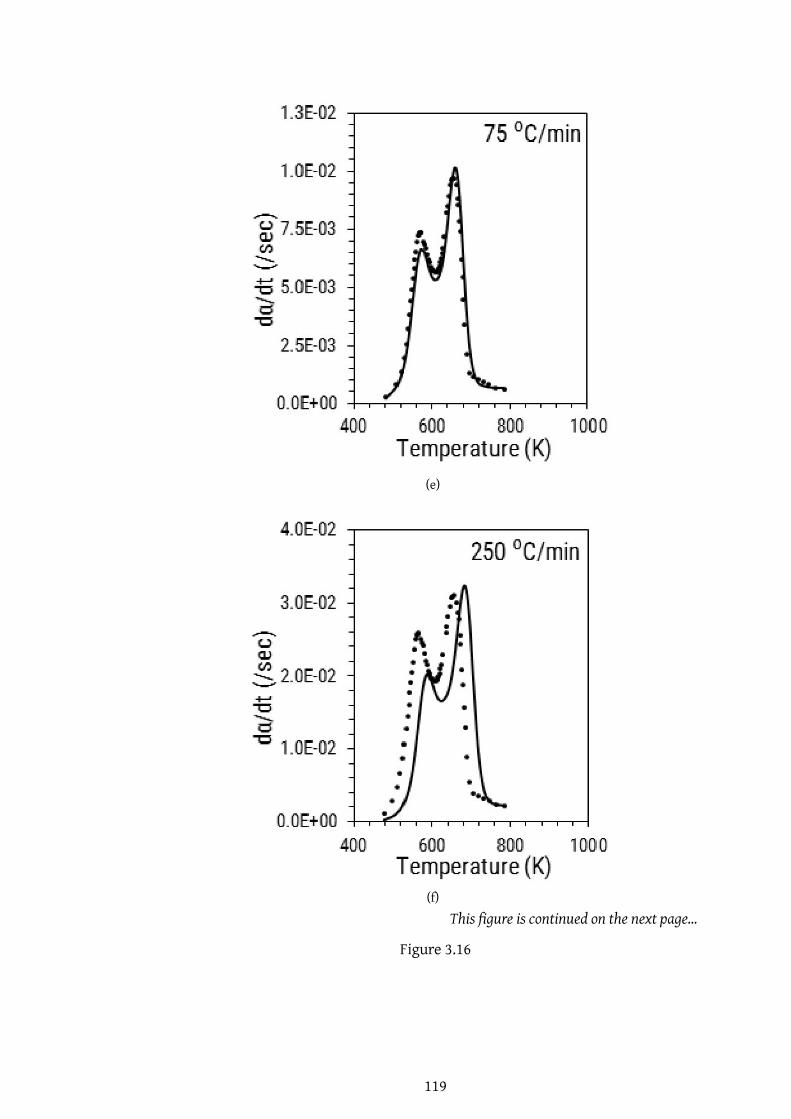
(e)

(f)

This figure is continued on the next page...

Figure 3.16

119

(g)

(h)

This figure is continued on the next page...

Figure 3.16

120

(i)

Figure 3.16: Comparison of experimental and predicted curves for different heat-ing rates. Predicted curves are obtained by using optimized DAEM parameters for(a) Case 2 (b) Case 2A and (c) Case 2B

3.6.4.5 Prediction of TGA curve at 1000 ◦C/s

DAEM equations and optimized parameters obtained here describe various mass

transfer processes that occur during biomass volatilization. As discussed in sec-

tions 3.6.2.3 and 3.6.4.4 heating rate has a profound effect on the morphology of

biomass particle and hence affects the volatilization rate. Biomass pore struc-

ture changes at high heating rates, and thus, similar changes might occur under

fast pyrolysis conditions. The DAEMparameterswere optimized under conditions

where morphological changes significantly affect mass loss rate. Thus, these pa-

rameters were used to predict biomass pyrolysis profile under 1000 ◦C/s or fast

pyrolysis conditions. Three different reaction models were used to predict the

volatilization curves obtained for pine, pine nut shell, rice husk, and rice straw

at 1000 ◦C/s using a wire mesh reactor [23]. The mass loss data was converted to

conversion (α) based on the final residue remaining at the end of pyrolysis. The

DAEMparameters used for predicting the curves are as shown in Table 3.15. These

121

parameters were optimized using biomass of particle size between 75 to 106 µm

and heating rates of 150 to 250 ◦C/min. An important observation from Figure

3.17 is that while the parameters were obtained for mallee wood, the predicted

curves for pine, and pine nut shell are in fair agreement with the experimental

data. One possible reason for such an agreement is similar ash content for pine,

pine nut shell, and the mallee biomass used. On the other hand, the mass loss

prediction for rice straw and husk is poor because the ash content for these raw

materials is around 15 wt.% [23] while that for the mallee biomass is around 1.3

wt.%. This demonstrates that the DAEM parameters derived using TGA at low

heating rates can predict volatile evolution profile under high heating rate condi-

tions if the model parameters take into consideration the effect of morphological

changes occurring during pyrolysis reaction.

Table 3.15: DAEM parameters optimized for three reactionmodels using pyrolysiscurves obtained for biomass particle size between 75 to 106 µm at heating ratesbetween 150 to 250 ◦C/min

ReactionModel

wc2-Gaussain modelweight fractions

E0(kJ/mol)

σ(kJ/mol)

log(A0)(sec−1) m obj func (J)

F1 0.1283 189.616 39.162 6.852 0.9859 0.04020.2655 226.308 8.632 17.4550.6062 0.4075 162.963 10.131 11.928

0.5925 175.007 2.212

DP 0.1230 189.458 39.812 8.581 0.4460 0.04980.2988 226.274 9.613 19.1620.5782 0.5690 164.663 7.975 11.721

0.4310 174.267 3.153

A2 0.1903 189.322 37.092 11.065 0.3883 0.06800.2445 226.848 8.860 19.5040.5652 0.5677 164.505 8.678 12.080

0.4323 175.113 4.166

122

(a)

(b)

This figure is continued on the next page...

Figure 3.17

123

(c)

(d)

This figure is continued on the next page...

Figure 3.17

124

(e)

(f)

This figure is continued on the next page...

Figure 3.17

125

(g)

(h)

This figure is continued on the next page...

Figure 3.17

126

(i)

(j)

This figure is continued on the next page...

Figure 3.17

127

(k)

(l)

Figure 3.17: Prediction of TGA curves using F1, DP and A2 reaction models for (a)to (c) pine, (d) to (f) pine nut shell, (g) to (i) rice husk and (j) to (l) straw pyrolysisunder 1000 ◦C/s

128

3.7 Summary

DAEMwasused as a lumpedmodel to describe the effect ofmorphological changes,

which occur during pyrolysis, on apparent volatilization rate of biomass. The ef-

fect of three particle sizes (≤45µm, 75 to 106 and 300 to 425µm) and seven heating

rates (5 to 250◦C/min) on biomass pyrolysis profile was studied using TGA, SEM

and optical microscope images. SEM images showed that heating rates chosen in

this study lead to significant physical changes in structure of biomass particles

which in turn affect the biomass volatilization profile. Formation of large bubbles

was observed on the surface of the biomass at heating rates beyond 75 ◦C/min

indicating presence of an intermediated molten phase. As the heating rates were

increased from 5-250 ◦C/min, an uneven temperature shift in TGA profile was ob-

served due to changes in pore structure of biomass. DAEM parameters - E0, A0,

m and σ for three pseudo-components were optimized for three reaction models

(first order, random scission and Avrami-Erofeev) to describe biomass pyrolysis

behavior. The parameter estimation procedure showed that it was essential to

separately optimize DAEM parameters to model the TGA profile at heating rates

greater than 150 ◦C/min because of significantmorphological changes in biomass.

Temperature dependence of frequency factor increased beyond heating rate of

150 ◦C/min because changes in pore structure became prominent after 300 ◦C

and 150 ◦C/min. The optimized DAEM parameters resulted in a fair prediction

of biomass volatilization under 1000 ◦C/s. This showed that the parameters can

be directly extrapolated to predict the behavior of biomass under fast pyrolysis

conditions in fluidized bed reactors where biomass particle size does not exceed

1 or 2 mm. Themodel can be improved further to include prediction of liquid, gas

and char yields is included.

129

Chapter 4

DAEM coupled detailed pyrolysis

kinetics

4.1 Introduction

Chapter 2 describes various biomass pyrolysis lumped kinetic models to predict

the gas, tar, and char yields. The distributed activation energy model was used

in Chapter 3 to predict the evolution rate of total pyrolysis volatiles and predict

char yield. However, to predict pyrolysis oil and gas composition, a detailed ki-

netic model is required. Kinetic model proposed by Ranzi et.al. [10] is capable

of predicting yields of major components present in pyrolysis gas and oil for any

biomass. The qualitative and quantitative predictions of any kinetic model de-

pend on the reaction steps considered in the model and value of kinetic param-

eters. Variables like biomass composition, temperature, and heating rate signifi-

cantly affect the nature of pyrolysis reactions. It is essential for the kinetic model

equations and parameters to be valid over a wide range of these variables. This

chapter therefore, compares the Ranzi model predictions for biomass pyrolysis of

different biomass types under wide range of heating rates (5 to 1000◦C/s). The

model is modified and coupled with distributed activation energy model (DAEM)

to improve predictability of gas, tar, and char yield along with the composition of

major gaseous and bio-oil components for biomass pyrolysis carried out different

heating rates.

Chapter 3 concludes that the morphological changes in mallee biomass become

130

prominent after heating rate of 150◦C/min and affect the evolution profile con-

siderably. Increase in heating rate of pyrolysis reaction reduces char yield and

increases gas and liquid yields. Heating rate also affects the bubble formation and

eruption during pyrolysis. At low heating rates, cross-linking reactions are dom-

inant, hence, intermediate liquid hardens and traps volatiles within the particle.

On the other hand at high heating rate the viscoelastic character of biomass par-

ticle is maintained which leads to volatile release via bubble eruption or aerosol

ejection due to pressure build-up. Viscoelastic or rigid nature of biomass particle

under pyrolysis conditions is dictated by the biomass type and heating rate [194].

Rigidity/elasticity of biomass particle affects the mobility of polymer chains, rad-

ical species, and other reactive intermediates which in turn affects the rate of

formation of tar, gas, and char species. To incorporate the effect of morphologi-

cal changes on rate of formation of different pyrolysis species, the detailed kinetic

scheme is coupled with the DAEM approach in this chapter.

4.2 Mathematical model

4.2.1 Detailed lumped kinetic model: Ranzi model

Ranzi model is a detailed lumped kinetic model, which is more mechanistic than

conventional lumped kinetic models. The main features of the model are (i) char-

acterization of the biomass structure, (ii) biomass devolatilization process, which

forms pyrolysis gas, liquid and char (29 reactions and 50 species), (iii) secondary

gas phase reactions of evolved volatile and gas species (20,239 reactions and 507

species). To simplify the model, pyrolysis reactions of cellulose, hemicellulose,

and lignin are assumed to proceed independently of one another other. Pyrolysis

is assumed to be a linear combination of the three pseudo components accord-

ing to their molar proportion. The reactions considered in this chapter are the

primary pyrolysis reactions, where solid biomass is converted to gas, liquid, and

char. Gas/vapor phase reactions occurring outside the biomass particle are not

considered, because the literature data for devolatilization used here is such that

secondary gas phase reactions are minimized. The secondary gas phase reactions

become important in reactor modeling.

131

4.2.1.1 Biomass chemistry

Chapter 2 describes the different components of lignocellulosic biomass. Chemi-

cal structure and relative content of cellulose, heimcellulose, lignin, and ash dif-

fers form one another and also with biomass type. Ranzi model [10] character-

izes biomass as a mixture of seven pseudo components. Structure of the pseudo-

components is shown in Figure 4.1. Cellulose is themost dominant polysaccharide

in plant cell wall and constitutes 15 to 50 wt% of dry plant material. It is a linear

polymer made up of β-1,4 linked glucopyranose units. Degree of polymerization

(DP) of cellulose is between 10 to 15 thousand glucopyranose units. Hemicellu-

lose is a amorphous branched hetero-polysaccharide that constitutes 25-30 wt%

of dry plantmaterial. Hexose and pentose units such as xylose, arabinose, glucose,

mannose, and galactose make up the hemicellulose polymer. Xylans are linear

homoxylan polysaccharides have β-1,3 and β-1,4 linkages, and L-arabinose side

chains are present in cell wall of cereal grains. Second class of hemicellulose com-

prises ofmannans- galactomannan, glucomannan, andgalacto-glucomannan. Glu-

comannan is a major component of softwood hemicellulose and less abundant in

hardwood and grasses. Hemicellulose has a DP of 70-200 units, with high molecu-

lar weight in hardwoods as compared to that in softwoods. Structure of cellulose,

xylan, and glucomannan repeating units is shown in Figure 4.1.

Lignin is a complex phenolic polymer with p-hydroxyphenyl (H), guaiacyl (G),

and syringyl (S) propanoid units as the main building blocks. Hardwood lignin

is pre-dominantly made up of guaiacyl and syringyl units with trace amount of p-

hydroxyphenyl units. Softwoods are mainly composed of guaiacyl units and low

amounts of p-hydroxyphenyl units. H-units content is slightly higher in grasses.

Characteristic inter-unit linkages in lignin are shown in Figure 4.2. The β-O-4

linkage makes up 46 to 60% of all the linkages [195]. As discussed in section 2.3.2,

LIG-H, LIG-O, and LIG-C (Figure 4.1) represent different repeating units with char-

acteristic linkages of lignin. The proportion of each repeating moiety changes

based on the type of biomass subjected to pyrolysis.

Extractiveswere not considered to characterize biomass in the Ranzimodel. How-

ever, complete characterization of several biomass species is not possible if only

cellulose, hemicellulose, and lignin are considered. Distribution of the extractives

132

Figure 4.1: Pseudo components used to model biomass pyrolysis kinetics

in plant material is different in various plant organs, most abundant in leaves and

bark. There are a wide range of extractives in plants, thus, Dibiagi et.al. [196]

broadly classified them into hydrophilic and hydrophobic type. Softwood species

contain upto 15 wt.% and hardwood samples contain <2 wt.% of hydrophobic

extractives. The most common hydrophobic extractive in plants is triglyceride

compound with high presence of linoleic acid [196]. Therefore, triglyceride (TGL:

C57H100O7) is used as a reference specie in the model. Hydrophilic extractives can

be further classified into flavonoids and non-falvonoids, latter being abundant

in plant material and include phenolic acids and tannins. Tannins are polyphe-

nolic compounds and condensed tannins (TANN: C15H12O7) is used to represent

hydrophilic extractives. As shown in Figure 4.3 (a) consideration of extractives as

a part of RM-2 and RM-3 mixture species allows the Ranzi model to characterize a

wider range of biomass species (hardwood, softwood, and grass type) as compared

to a case in which extractives are not used as pseudo-components.

133

Figure 4.2: Representative chemical structure of lignin with different bond link-ages [22]

The pyrolysis chemistry of cellulose, hemicellulose, lignin, and extractives is dif-

ferent, hence the first step in biomass pyrolysis modeling is specifying reference

species which can represent different biomass components. If information on

biochemical composition is unavailable, the reference specie composition can be

determined using elemental analysis of biomass. H/C/O atomic balances allow

to evaluate a suitable combination of three reference species (RM-1, RM-2, and

RM-3). These three mixture species are further composed of Cell, Hcell, LIG-O,

LIG-C, LIG-H, TGL, and TANN using mole fractions/splitting parameters nα, nβ ,

nγ , nδ, and nε. RM-1 is representative of hollocellulose, whereas RM-2 and RM-3

are mixture of lignin and extractives (Figure 4.3). The value of splitting param-

eters are defined from experimental findings and can be modified to establish

elemental balance.

Calculation ofmixture species and internal composition ofmixture species for dif-

ferent biomass samples is shown in Table 4.1. Themole fractions RM-1, RM-2, and

RM-3 are estimated based on the H/C/O balance of the rice straw, rice husk, and

pine nutshell reported in [23] and of pine wood reported in [122]. In this study,

if the biochemical composition of a biomass specie is not reported, initial guess

134

(a) (b)

Figure 4.3: Combining biomass pseudo components into three mixtures- RM-1,RM-2, and RM-3 [10]. The scatter points in figure (a) shows composition of differ-ent softwood, hardwood, and grass biomass species.

of splitting parameters is based on the database published by Debiagi et.al. [196],

where biochemical, elemental, and ash analysis of more than 600 lignocellulosic

biomass species is published along with estimates of splitting parameters. Us-

ing the value of splitting parameters, the H/C/O composition of mixture species

RM-1, RM-2, and RM-3 is determined. The value of splitting parameters and com-

position of mixture species is adjusted to establish elemental balance.

135

Table4.1:Estimatedvaluesofbiomasspseudo-componentsoffourbiomassspeciesusingRanzimodelcharacterization.Thepseudo-component

compositionisreportedinmolefraction

Components

Rice

Straw[23]

Rice

husk[23]

Pine

nutshell[23]

Pine[122]Spruce[24]

Oak[24]

Pine[24]

Cell

0.4304

0.4451

0.4444

0.4462

0.5712

0.5060

0.5456

XYHW/GMSW

0.3788

0.3642

0.2945

0.3697

0.2704

0.3148

0.2871

LIGC

0.0176

0.0377

0.1029

0.0297

0.0527

0.0338

0.0220

LIGH

0.0004

0.0007

0.1122

0.0416

0.0144

0.0934

0.0220

LIGO

0.1215

0.1503

0.0313

0.0773

0.0889

0.0419

0.0869

TGL

0.0024

0.0020

0.0128

0.0016

0.0024

0.0000

0.0000

TANN

0.0487

0.0000

0.0019

0.0340

0.0000

0.0100

0.0363

RM-1

0.8092

0.7992

0.7389

0.8158

0.8417

0.8208

0.8327

RM-2

0.0029

0.0023

0.1329

0.0535

0.0172

0.1168

0.0275

RM-3

0.1879

0.1985

0.1282

0.1306

0.1411

0.0624

0.1398

alpha

0.5319

0.5500

0.6014

0.5469

0.6787

0.6165

0.6552

beta

0.9100

0.8000

0.9343

0.8000

0.9700

0.8000

0.8000

gamma

0.8736

0.8000

0.2475

0.8000

0.6300

0.8000

0.8400

delta

0.1700

0.2900

0.9038

0.9700

0.8600

1.0000

1.0000

136

Table4.1continuedfrom

previouspage

Components

Rice

Straw[23]

Rice

husk[23]

Pine

nutshell[23]

Pine[122]Spruce[24]

Oak[24]

Pine[24]

epsilon

0.7405

1.0000

0.9851

0.7400

1.0000

0.8400

0.7400

Experiment

C(dafwt%)

0.4966

0.5050

0.5320

H(dafwt%)

0.0583

0.0537

0.0601

O(dafwt%)

0.4451

0.4412

0.4079

Cellulose

(drywt%)

3547.1

±0.4

43.2

±0.3

45.6

±0.1

Hemicellulose

(drywt%)

2922.3

±0.4

21.9

±0.7

24.0

±0.7

Lignin

(drywt%)

2829.2

±0.6

35.4

±0.4

26.8

±0.3

Extractives

(drywt%)

1.1±0.4

35.4

±0.5

26.8

±0.4

137

Table4.1continuedfrom

previouspage

Components

Rice

Straw[23]

Rice

husk[23]

Pine

nutshell[23]

Pine[122]Spruce[24]

Oak[24]

Pine[24]

Prediction

C(dafwt%)

0.5012

0.5047

0.5285

H(dafwt%)

0.0580

0.0586

0.0639

O(dafwt%)

0.4409

0.4367

0.4076

Cellulose

(drywt%)

35.71

47.24

42.31

44.66

Hemicellulose

(drywt%)

29.59

22.37

21.45

23.51

Lignin

(drywt%)

28.87

29.29

34.67

26.25

Extractives

(drywt%)

5.80

1.1

1.57

5.58

138

4.2.1.2 Reaction chemistry

The reactions of pseudo-components are tabulated in Table 4.2. Polymeric cel-

lulose, hemicellulose, and lignin species undergo end and mid chain depolymer-

ization to form non-volatile oligomeric/polymeric active species along with the

release of smallmolecules likewater, and other pyrolysis gases. The active species,

CellA, HCE-1, HCE-2, LIGCC, LIG, and LIGOH further depolymerize and cross-link to

form gas, tar and char. Cellulose pyrolysis is assumed to follow a simple reaction

pathwith focus on formation of typical products like levoglucosan (LVG), hydroxy

acetaldehyde (HAA), and hydroxy methyl-furfural (HMFU). Active cellulose and

char are formed from through two competing cellulose pyrolysis reactions. Active

cellulose further evolves through two competitive pathways: end-chain scission

to yield LVG and β-scission reactions inside polymer chain with subsequent dehy-

dration, isomerization, retro Diels-Alder, and tautomerization reactions to form

glyoxal, acetaldehyde, formic acid, HMFU, CO, CO2 and other light products. The

stoichiometric coefficients are based on mechanistic, experimental, and theoret-

ical works reported in [123, 107, 197].

139

Table4.2:Ranzimodelforbiomasspyrolysis[27]

Sr.

no.

Reactant

Product

E,kJ/mol;

A,s−

1

Cellulose

R1Cell

→CellA

1.5x10

14xexp(-196.648/RT)

R2CellA

→0.4HAA

+0.05GLYOX+0.15CH

3CHO+0.25HMFU+0.35ALD3

+0.15CH

3OH+0.3CH

2O+0.61CO+0.36CO

2+0.05H

2

+0.93H

2O+0.02HCOOH

+0.05C 3H

6O2+0.05T(CH

4)

2.5x10

6xexp(-79.914/RT)

R3CellA

→LVG

3.3xTxexp(-41.840/RT)

R4Cell

→5H

2O+6CHAR

6x10

7xexp(-129.704/RT)

Hemicellulose

R5GM

SW→

0.70HCE1+0.30HCE2

1x10

10xexp(-129.704/RT)

R6XYHW

→0.35HCE1+0.65HCE2

1x10

10xexp(-119.244/RT)

R7HCE1

→0.60XYLAN

+0.20C 3H

6O2+0.12GLYOX+0.20FURF+0.40H

2O

+0.08T(H

2)+0.16CO

3xTxexp(-46.024/RT)

140

Table4.2continuedfrom

previouspage

Sr.

no.

Reactant

Product

E,kJ/mol;

A,s−

1

R8HCE1

→0.4H

2O+0.79CO

2+0.05HCOOH

+0.69CO+0.01T(CO)+0.01T(CO

2)

+0.35T(H

2)+0.3CH

2O+0.9T(COH

2)+0.625T(CH

4)+0.375T(C 2H

4)

+0.875CHAR

1.8x10

−3xTxexp(-12.552/RT)

R9HCE2

→0.2H

2O+0.275CO+0.275CO

2+0.4CH

2O+0.1C 2H

5OH+0.05HAA

+0.35ACAC+0.025HCOOH

+0.25T(CH

4)+0.3T(CH

3OH)

+0.225T(C 2H

4)+0.4T(CO

2)+0.725T(COH

2)

5x10

9xexp(-131.796/RT)

Lignin

R10

LIGC

→0.35LIGCC+0.10COUMARYL+0.08PHENOL+0.41C 2H

4+H

2O

+0.70T(COH

2)+0.30CH

2O+0.32CO+0.495T(CH

4)

1x10

11xexp(-155.644/RT)

R11

LIGH

→LIGOH+0.50ALD3+0.50C 2H

4+0.20HAA

+0.10CO+0.10T(H

2)6.7x10

12xexp(-156.900/RT)

R12

LIGO

→LIGOH+CO

23.3x10

8xexp(-106.692/RT)

R13

LIGCC

→0.30COUMARYL+0.20PHENOL+0.35HAA

+0.70H

2O+0.65CH

4

+0.60C 2H

4+H

2+1.40CO+0.4T(CO)+6.75CHAR

1x10

4xexp(-103.763/RT)

141

Table4.2continuedfrom

previouspage

Sr.

no.

Reactant

Product

E,kJ/mol;

A,s−

1

R14

LIGOH

→0.90LIG+H

2O+0.1CH

4+0.60CH

3OH+0.05T(H

2)+0.3T(CH

3OH)

+0.05CO

2+0.65CO+0.6T(CO)+0.05HCOOH

+0.85T(COH

2)

+0.35T(CH

4)+0.20T(C 2H

4)+4.25CHAR

1x10

8xexp(-125.520/RT)

R15

LIG

→0.70FE2MACR+0.30ANISOLE+0.30CO+0.30T(CO)

+0.30CH

3OH

4xTxexp(-50.208/RT)

R16

LIG

→0.60H

2O+0.40CO+0.20CH

4+0.4CH

2O+0.20T(CO)+0.40T(CH

4)

+0.50T(C 2H

4)+0.40T(CH

3OH)+2T(COH

2)+6CHAR

8.3x10

−2xTxexp(-33.472/RT)

R17

LIG

→0.60H

2O+2.6CO+1.1CH

4+0.40CH

2O+C 2H

4

+0.40CH

3OH

1x10

7xexp(-101.671/RT)

Extractives

R18

TGL

→ACROL+3FFA

7x10

12xexp(-191.208/RT)

R19

TANN

→0.85PHENOL+0.15T(PHENOL)+T(CO)+H

2O+ITANN

2x10

1xexp(-41.840/RT)

R20

ITANN

→5CHAR

+2CO+H

2O+T(COH

2)1x10

3xexp(-104.600/RT)

142

Table4.2continuedfrom

previouspage

Sr.

no.

Reactant

Product

E,kJ/mol;

A,s−

1

Metaplastreactions

R21

T(CO

2)→

CO2

1x10

6xexp(-100.416/RT)

R22

T(CO)

→CO

5x10

12xexp(-209.200/RT)

R23

T(COH

2)→

COH

21.5x10

12xexp(-297.064/RT)

R24

T(H

2)→

H2

5x10

11xexp(-313.800/RT)

R25

T(CH

4)→

CH4

5x10

12xexp(-299.156/RT)

R26

T(CH

3OH}

→CH

3OH

2x10

12xexp(-209.200/RT)

R27

T(C 2H

4)→

C 2H

45x10

12xexp(-299.156/RT)

R28

T(PHENOL)

→PHENOL

1.5x10

12xexp(-297.064/RT)

Moisturevaporization

R29

ACQUA

→H

2O1xTxexp(-33.472/RT)

143

Hemicellulose is a branched polymer and has a more complicated structure than

cellulose with hexose and pentose sugars as backbonewith o-acetyl groups as side

groups. Two different pseudo-components for hemicellulose are considered in

the Ranzimodel for hardwood (xylose based, XYHW) and softwood (glucomannan

based, GMSW). The two intermediate species HCE-1 andHCE-2 represent different

composition of hardwood and softwood hemicellulose. Hardwood hemicellulose

typically yields more char as compared to softwood hemicellulose, which is con-

sidered in HCE1 decomposition. Typical hemicellulose pyrolysis products include

furfural, acetol, formic acid, acetic acid, furfuryl alcohol, acetone, and permanent

gases. The nature of hemicellulose pyrolysis reactions is similar to that of cellu-

lose.

Lignin structure is more complicated than cellulose and hemicellulose. The reac-

tion chemistry of ether (β-O-4) and C-C bond (Cα-Cβ) in the syringol and guaiacyl

units (Figure 4.2) plays important role during lignin pyrolysis. The multistep ki-

netic scheme of lignin is a simplification of detailed lignin pyrolysis scheme pro-

posed by Faravelli et al. [92]. Beyond 200◦C, lignin pyrolysis is amolten phase rad-

ical process with competing initiation, propagation, and termination reactions of

different propagating radicals. LIG-O and LIG-H have methoxy groups on phenyl

ring adjacent to the ether linkage which decreases the bond dissociation energy

of β-O-4 in comparison to LIG-C that does not have any substituent on the phenyl

ring. Therefore, the lignin constituents are differentiated from one another as

they undergo reactions with different energetics during pyrolysis. Lignin pyrol-

ysis reactions used by Faravelli et al.[92] are represented in Figure 4.4. Faravelli

model uses 100 radical and molecular species and 500 elementary and lumped re-

actions to describe lignin pyrolysis. In the Ranzi model the reactions are further

lumped to 8 reactions as shown in Table 4.2. Condensible products for lignin py-

rolysis model are coumaryl alcohol, sinapyl aldehyde (FE2MACR), phenol, anisole,

hydroxyacetaldehyde, formic acid, methanol, formaldehyde, and propenal.

Pyrolysis of the extractives is explained using three lumped reactions. Tannins

undergo pyrolysis in two steps, first one is a volatilization reaction occurring

between 125 to 300◦C and the second one being a condensation/charring reac-

tion with less release of volatile species [198–200]. Ranzi model therefore, con-

144

Figure 4.4: Different free radical reactions for lignin

145

siders a two-step decomposition of TANN, with maxmimum mass loss between

280-310◦C, producing phenolic specie and an intermediatemetaplast/solid specie

ITANN (3,5- dihydroxy benzofuranone: C9H6O6). ITANN then degrades to gas and

predominantly char via slow decarbonylation, dehydration and charring reaction

[196]. TGL pyrolysis is based on the studies of soyabean and corn oil, which when

used as mixture better represent real biomass. Acrolein (C2H3CHO) and fatty acid

(FFA, C18H32O2) are the pyrolysis products of TGL, with negligible char [201]. Thus,

the Ranzi model uses one reaction that produces acrolein and FFA at about 350◦C.

Ranzi model also includes reactions for the release of gases/volatiles trapped in-

side the intermediate liquid formed during pyrolysis. The resistance for the re-

lease of gases is expressed in the form of Arrhenius type equation. These reac-

tions are included to account for the effect of intermediate melting on the release

of volatile species formed during pyrolysis.

Ash (salt ions like K, Na, Ca, and Mg) acts as a catalyst in the pyrolysis processes

and reduces the yield of organics from pyrolysis liquid with increase in water and

char content [28, 202, 203]. Metal cations favour the formation of light oxygenates

like aldehydes and carboxylic acids from sugars over depolymerization of polysac-

charide chains [204]. Metal cations like Ca promote the formation of primary and

secondary char, and light oxygenates from sugars like levoglucosan. The effect

of ash on the nature of pyrolysis reactions is complete approximately beyond 5

wt.%. In other words, ash content greater than 5 wt.% (of biomass) does not have

additional effect on the yield of pyrolysis char and liquid [10]. To consider the

effect of ash a global dimensionless ash factor (AF, Eq.(4.1)) with values between

0 (no ash) and 1 (≥5 wt.%). Ranzi model considers the effect of ash on the activa-

tion energy of R2, R4, and R8 (Table 4.2) as shown in Eq.(4.2) to Eq.(4.4). If the ash

content of biomass is≤1 wt.%, value of AF becomes 0.5. Thus, the activation en-

ergies tabulated in Table 4.2 are valid for ash content≤1 wt.%. If the ash content

exceeds 5 wt.%, value of x in the Eq.(4.2) to Eq.(4.4) is substituted as 5.

146

AF = tanh

(ash

2

)(4.1)

E2 = 19100 − 600x(AF − 0.5) (4.2)

E4 = 31000 − 1000x(AF − 0.5) (4.3)

E8 = 3000 − 1000x(AF − 0.5) (4.4)

4.2.2 DAEM coupled modified Ranzi model

Although the Ranzi model is capable of predicting the composition of gas andma-

jor liquid species, it still has some limitations. The model does not predict the

formation of cresols, guaiacol/methyl guaiacol, dimethoxy phenol, vinyl phenol,

and eugenol, which are major constituents of bio-oil (Table 2.4). The model uses

a relatively simple scheme for cellulose pyrolysis and considers only mid-chain

cleavage of cellulose, because formation of active cellulose is not accompanied

with levoglucosan formation. In the mechanistic model proposed by Zhou et. al.

[107], end chain cleavage of cellulose yields both active cellulose and levoglucosan.

As discussed in Chapter 3, using a unique value of activation energy may not be a

good description of solid decomposition rate. Also, chemical and physical struc-

ture of biomass particle changes continuously during pyrolysis, which strongly

depends on the heating rate. The next section gives a theoretical background of

the modifications made to the Ranzi model (Mo-Ranzi) and the justification for

coupling it with DAEM.

4.2.2.1 Model modification: Theoretical background

Heating rate affects the plasticization of biomass particle as shown in chapter 3.

The plasticization is stronger at high heating rates as compared to that at low

heating rates [194]. Cellulose and hemicellulose, with weak hemi-acetal bonds,

147

and lignin are known to undergo partial melting at high heating rates [205, 73,

112]. Heating rates affect the melting and expansion of biomass particle, which

in turn affect the bond-scission, cross-linking, and intra-particle mass transfer of

volatiles. Under slow heating rates, cross-linking hinders the melting of biomass

particle thereby decreasing its plasticity. On the other hand at high heating rate,

bond-breaking reactions dominatewhile cross-linking isminimized, thus, impart-

ing fluidity to biomass particle. Extent of fluidity also depends on the oxygen and

ash content of biomass. For example, herbaceous biomass have high oxygen con-

tent, which can lead to low temperature cross-linking reactions and reduce the

fluidity at high heating rates when compared to woody biomass. Minerals like K

and Ca can also promote polymerization reactions thereby generating char and

reducing plasticity [194].

Plasticity of particle imparts additional mobility to polymer chains, intermediate

radicals, and small non-volatilemolecules formed during pyrolysis. The increased

mobility can increase the collision frequency of reacting molecules with one an-

other, thus, increasing the probability of conversion. Electron spin resonance

spectroscopy analysis results of char obtained under same pyrolysis conditions

show presence of free radicals in solidified char of wheat straw and rice husk,

but there are no free radicals remaining in wood and ash leached wheat straw

chars [194]. Since the wood and ash leached wheat straw are deprived of ash,

biomass particle have sufficient fluidity to allow recombination of radicals and

formation of polyaromatic structure. On the other hand presence of ash in wheat

straw and rice husk increases cross-linking reactions and hinders the mobility of

free radicals to recombine to form char or propagate to form tar molecules and

intermediates. Effect of such a phenomenon on biomass conversion rate can be

accounted for bymodifying the frequency factor of a reaction by adding a correc-

tion factor (Table 4.3) that depends on heating rate of pyrolysis reaction. Change

in the correction factor with respect to heating rate is shown in Figure 4.5. Effect

of biomass fluidity on conversion would reach a limit because biomass particle

does not melt completely. Different coefficients are assigned to cellulose, hemi-

cellulose, and lignin. Char yield decreases in the order: lignin > hemicellulose >

cellulose. Lignin pyrolysis proceeds through radical formation which further de-

148

compose to tar molecule or recombine to form char. Therefore, in most of the re-

actions describing lignin pyrolysis char and tar are co-produced. Hemicellulose is

amorphous and more reactive than cellulose. Further effect of ash on hemicellu-

lose pyrolysis ismore profound because inorganic species are associatedwith glu-

curonic acid units [206]. Hence, different coefficients are assigned to char forming

and volatilization reactions.

Figure 4.5: Correction factor profile with respect to heating rate

Activation energy of each reaction in Table 4.3 is assumed to followGaussian prob-

ability distribution. The model assumes that biomass pyrolysis is a linear com-

bination of pseudo-components described in section 4.2.1. The composition of

biomass particle at molecular level also changes spatially. So, change in molecu-

lar environment leads to change in the activation energy of a given reaction. Fur-

ther, lignin pyrolysismodels have been formulated based on lignin extracted from

biomass. The degree of polymerization and structure of extracted lignin is differ-

ent than native lignin. Also, as described in Chapter 3, DAEM can be used to de-

scribe the effect of morphological changes on the resistance of biomass volatiliza-

tion process. Although Ranzi model considers separate reactions for release of

trapped gases, but evolution of other tar/liquid species can also be affected by

149

physical changes in pore structure of biomass. Therefore, DAEM coupling with

each reaction accounts for the effect of changing morphology and molecular en-

vironment of biomass particle during pyrolysis.

Finally, reactionsMR5,MR13, andMR17 are added to the original Ranzimodel. Re-

action MR5 accounts for end chain cleavage of cellulose polymer based on mech-

anistic model proposed by Zhou et.al.[107]. Also, furfural is added as one of the

product in reaction MR2, because furfural forms through triple dehydration of

fructose, where the latter is an isomerization product of glucose. The activation

energy and frequency factor of MR1 and MR5 is also adopted from the cellulose

mechanistic model. Experimental data show that along with dianhydro xylopy-

ranose (DAXP), xylose is also one of the pyrolysis products of hemicellulose [62].

Therefore, along with DAXP, (considered int he Ranzi model) xylose is also incor-

porated as one of the hemicellulose pyrolysis products in MR8. MR13 and MR17

are added based on the detailed ligninmodel proposed by Faravelli et.al.[92] to in-

corporate major monomeric pyrolysis products of lignin (High molecular weight

lignin, KETM2, methyl guaiacol, sinapyl alcohol, propionic acid). A list of species

used in the Ranzi and modified Ranzi model are reported in Table 4.4.

150

Table4.3:ModifiedRanzimodelcoupledwithDAEM

forbiomasspyrolysis

Sr.

no.

Reactant

Product

E,kJ/mol;

A,s−

1σ

Correction

Factor

Cellulose

MR1

Cell

→CellA

1.5x10

14xexp(-223.844/RT)

σM

R1

1/(v

log(H

R)

Cel

l)

MR2

CellA

→0.4HAA

+0.05GLYOX+0.15CH

3CHO+0.25HMFU+0.35ALD3+

0.0805FURF+0.15CH

3OH+0.3CH

2O+0.61CO+0.36CO

2+

0.05H

2+0.93H

2O+0.02HCOOH

+0.05C 3H

6O2+0.05T(CH

4)

2.5x10

6xexp(-79.914/RT)

σM

R2

1/(v

log(H

R)

Cel

l)

MR3

CellA

→LVG

3.3xTxexp(-41.840/RT)

σM

R3

1/(v

log(H

R)

Cel

l)

MR4

Cell

→5H

2O+6CHAR

6x10

7xexp(-129.704/RT)

σM

R4

1/(c

log(H

R)

Cel

l)

MR5

Cell

→0.5CellA+0.5LVG

3x10

15xexp(-215.476/RT)

σM

R5

1/(v

log(H

R)

Cel

l)

Hemicellulose

MR6

GMSW

→0.70HCE1+0.30HCE2

1x10

10xexp(-129.704/RT)

σM

R6

1/(v

log(H

R)

HC

ell)

MR7

XYHW

→0.35HCE1+0.65HCE2

1x10

10xexp(-119.244/RT)

σM

R7

1/(v

log(H

R)

HC

ell)

MR8

HCE1

→0.30XYLAN

+0.347DAXP+0.20C 3H

6O2+0.12GLYOX+

0.20FURF+0.40H

2O+0.08T(H

2)+0.16CO

3xTxexp(-46.024/RT)

σM

R8

1/(v

log(H

R)

HC

ell)

151

Table4.3continuedfrom

previouspage

Sr.

no.

Reactant

Product

E,kJ/mol;

A,s−

1σ

Correction

Factor

MR9

HCE1

→0.4H

2O+0.79CO

2+0.05HCOOH

+0.69CO+0.01T(CO)+

0.01T(CO

2)+0.35T(H

2)+0.3CH

2O+0.9T(COH

2)+

0.625T(CH

4)+0.375T(C 2H

4)+0.875CHAR

1.8x10

−3xTxexp(-12.552/RT)

σM

R9

1/(c

log(H

R)

HC

ell)

MR10

HCE2

→0.2H

2O+0.275CO+0.275CO

2+0.4CH

2O+

0.1C 2H

5OH+0.05HAA

+0.35ACAC+0.025HCOOH

+

0.25T(CH

4)+0.3T(CH

3OH)+0.225T(C 2H

4)+

0.4T(CO

2)+0.725T(COH

2)+0.6336CHAR

5x10

9xexp(-131.796/RT)

σM

R10

1/(c

log(H

R)

HC

ell)

Lignin

MR11

LIGC

→0.35LIGCC+0.201COUMARYL+0.16PHENOL+0.41C 2H

4+

H2O+0.70T(COH

2)+0.30CH

2O+0.32CO+0.496T(CH

4)+

3.844CHAR

1x10

11xexp(-155.644/RT)

σM

R11

1/(v

log(H

R)

Lig

nin)

MR12

LIGH

→LIGOH+0.50ALD3+0.50C 2H

4+0.20HAA

+

0.10CO+0.10T(H

2)

6.7x10

12xexp(-156.900/RT)

σM

R12

1/(v

log(H

R)

Lig

nin)

152

Table4.3continuedfrom

previouspage

Sr.

no.

Reactant

Product

E,kJ/mol;

A,s−

1σ

Correction

Factor

MR13

LIGH

→0.24HMWL+0.28KETM2+0.39MGUAIA+0.35PHENOL+

1.2H

2O+0.4CO

2+0.25CO+0.2CH

2O+0.3CH

3OH+

0.5ALD3+0.306HAA

+0.2T(CH

3OH)+0.2T(CO)+

0.1T(CO

2)+5.251CHAR

1x10

9xTxexp(-166.73/RT)

σM

R13

1/(v

log(H

R)

Lig

nin)

MR14

LIGO

→LIGOH+CO

23.3x10

8xexp(-106.692/RT)

σM

R14

1/(v

log(H

R)

Lig

nin)

MR15

LIGCC

→0.30COUMARYL+0.20PHENOL+0.35HAA

+0.70H

2O+

0.65CH

4+0.60C 2H

4+H

2+1.40CO+0.4T(CO)+

6.75CHAR

1x10

4xexp(-103.763/RT)

σM

R15

1/(v

log(H

R)

Lig

nin)

MR16

LIGOH

→0.796LIG+H

2O+0.1CH

4+0.60CH

3OH+0.05T(H

2)+

0.3T(CH

3OH)+0.05CO

2+0.55CO+0.6T(CO)+0.054HCOOH

+

0.85T(COH

2)+0.35T(CH

4)+0.20T(C 2H

4)+4.15CHAR

1x10

8xexp(-125.520/RT)

σM

R16

1/(c

log(H

R)

Lig

nin)

MR17

LIGOH

→0.45SINAPYLALC+0.55MGUAIA+0.3PROPAC+0.978CH

3OH+

0.444H

2+0.4CO+11.1CHAR

1x10

9xTxexp(-163.176/RT)

σM

R17

1/(c

log(H

R)

Lig

nin)

MR18

LIG

→0.60FE2MACR+0.20ANISOLE+0.28MGUAIA+0.1CRESOL+

0.135DIMEPHENOL+0.582CO+0.30T(CO)+0.30CH

3CHO

4xTxexp(-50.208/RT)

σM

R18

1/(v

log(H

R)

Lig

nin)

153

Table4.3continuedfrom

previouspage

Sr.

no.

Reactant

Product

E,kJ/mol;

A,s−

1σ

Correction

Factor

MR19

LIG

→0.701H2O+0.467CO+0.234CH4+0.467CH

2O+0.234T(CO)+

0.467T(CH

4)+0.584T(C 2H

4)+0.467T(CH

3OH)+

2.336T(COH

2)+7.009CHAR

+0.234ALD3+0.054HCOOH

8.3x10

−2xTxexp(-33.472/RT)

σM

R19

1/(c

log(H

R)

Lig

nin)

MR20

LIG

→0.876H2O+3.795CO+1.606CH4+0.584CH

2O+

1.46C2H4+0.584CH

3OH+2.853CHAR

1x10

7xexp(-101.671/RT)

σM

R20

1/(c

log(H

R)

Lig

nin)

Extractives

MR21

TGL

→ACROL+3FFA

7x10

12xexp(-191.208/RT)

σM

R21

1/(v

log(H

R)

extr

act

ive)

MR22

TANN

→0.85PHENOL+0.15T(PHENOL)+T(CO)+H

2O+ITANN

2x10

1xexp(-41.840/RT)

σM

R22

1/(v

log(H

R)

extr

act

ive)

MR23

ITANN

→5CHAR

+2CO+H

2O+T(COH

2)1x10

3xexp(-104.600/RT)

σM

R23

1/(c

log(H

R)

extr

act

ive)

Metaplastreactions

MR24

T(CO

2)→

CO2

1x10

6xexp(-100.416/RT)

σM

R24

1/(v

log(H

R)

tra

p)

MR25

T(CO)

→CO

5x10

12xexp(-209.200/RT)

σM

R25

1/(v

log(H

R)

tra

p)

MR26

T(COH

2)→

CO+H

21.5x10

12xexp(-297.064/RT)

σM

R26

1/(v

log(H

R)

tra

p)

MR27

T(H

2)→

H2

5x10

11xexp(-313.800/RT)

σM

R27

1/(v

log(H

R)

tra

p)

154

Table4.3continuedfrom

previouspage

Sr.

no.

Reactant

Product

E,kJ/mol;

A,s−

1σ

Correction

Factor

MR28

T(CH

4)→

CH4

5x10

12xexp(-299.156/RT)

σM

R28

1/(v

log(H

R)

tra

p)

MR29

T(CH

3OH)

→CH

3OH

2x10

12xexp(-209.200/RT)

σM

R29

1/(v

log(H

R)

tra

p)

MR30

T(C 2H

4)→

C 2H

45x10

12xexp(-299.156/RT)

σM

R30

1/(v

log(H

R)

tra

p)

MR31

T(PHENOL)

→PHENOL

1.5x10

12xexp(-297.064/RT)

σM

R31

1/(v

log(H

R)

tra

p)

Moistureevaporation

MR32

ACQUA

→H

2O1xTxexp(-33.472/RT)

σM

R32

1/(v

log(H

R)

tra

p)

155

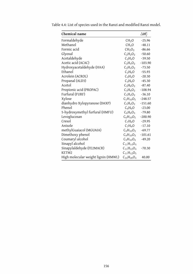
Table 4.4: List of species used in the Ranzi and modified Ranzi model.

Chemical name ∆H0f

Formaldehyde CH2O -25.96Methanol CH4O -48.11Formic acid CH2O2 -86.66Glyoxal C2H2O2 -50.60Acetaldehyde C2H4O -39.50Acetic acid (ACAC) C2H4O2 -103.90Hydroxyacetaldehyde (HAA) C2H4O2 -73.50Ethanol C2H6O -55.93Acrolein (ACROL) C3H4O -20.30Propanal (ALD3) C3H6O -45.30Acetol C3H6O2 -87.40Propionic acid (PROPAC) C3H6O2 -108.94Furfural (FURF) C5H4O2 -36.10Xylose C5H10O5 -248.57dianhydro Xylopyranose (DAXP) C5H4O2 -151.60Phenol C6H6O -23.005-hydroxymethyl furfural (HMFU) C6H6O3 -79.80Levoglucosan C6H10O5 -200.90Cresol C7H8O -29.95Anisole C7H8O -17.10methylGuaiacol (MGUAIA) C8H10O2 -69.77Dimethoxy phenol C8H10O3 -101.61Coumaryl alcohol C9H10O2 -49.20Sinapyl alcohol C11H14O4Sinapylaldehyde (FE2MACR) C11H12O4 -70.30KETM2 C11H12O5High molecular weight lignin (HMWL) C24H28O4 40.00

156

4.2.2.2 Model equations

All the reactions are assumed to followfirst order reaction kinetics. Each equation

is coupled with DAEM as shown below, The model equations for the coupling of

DAEM and Ranzi model are as

dxi

dt=

rxn∑j=1

∫ ∞

0

1CF

log(HR)comp

A0,jTmj exp

(−Ej

RT

)f(E)dE

spc∏i=1

Yi,jxνi,j (4.5)

f(E) = 1σj

√2π

exp

(−(Ej − E0,j)2

2σ2j

)(4.6)

Where, i and j specie and reaction number while rxn and spc are total number

of reactions and species; CF stands for correction factor (either v or c as given in

Table 4.3) comp signifies cellulose, hemicellulose, lignin, extractives, or trapped

species. xi is themass fraction of any species i. Yi,j is the coefficient for any specie

i and reaction j, and ν is the species order in any j reaction. f(E) is the Gaussian

function describing the probablistic distribution of activation energy for each re-

actionmentioned in Table 4.3. The values of frequency factor (A0,j), mean activa-

tion energy (E0,j), and temperature exponent (mj) are used as input parameters

(Table 4.3). The values of σj , vcomp, and ccomp are optimized using fmicon function

in MATLAB and the set of differential equations are solved using ode45 solver of

MATLAB.

4.3 Optimization of DAEM parameters and correc-

tion factor

Values of mean activation energy of each reaction assumed are stated in Table 4.3.

The activation energy of reactions R2, R4, and R9 were calculated based on the

ash content of biomass. The variance of Gaussian distribution and coefficients for

correction factors, totaling 40 parameters, were optimized using pattern search

algorithm (MATLAB2016). As the number of parameters was large, pattern search

algorithmwas chosen because it is faster than gradient specified fmincon (used in

157

Chapter 3). The literature data of rice straw, rice husk, and pine nutshell weight

loss under pyrolysis conditions with heating rates of 5 and 1000◦C/s [23] was used

for optimization. The optimized parameters are reported in Table 4.5. The pa-

rameters were optimized by minimizing the error between predicted and experi-

mental values simultaneously for 5 and 1000◦C/s. As, the number of variables for

optimization was large, the parameters were tested and adjusted so as to accu-

rately predict the oil, gas, and char yield of other biomass samples (spruce, oak,

and pine [24]) at different temperatures.

Table 4.5: Optimized DAEM parameters and correction factor coefficients

DAEM parameters Correction factor

σ ash≤1 wt.% ash≥5 wt.% Coefficients ash≤1 wt.% ash≥5 wt.%σMR1 10.10 10.10 vcell 0.5 0.20σMR2 6.09 6.09 ccell 2.8 1.10σMR3 2.19 2.19 vhcell 0.3 0.30σMR4 4.12 4.12 chcell 1.8 0.60σMR5 8.97 8.97 vlignin 0.15 0.15σMR6 6.42 6.42 clignin 0.1 0.15σMR7 7.35 7.35 vextractive 0.4 0.2σMR8 2.35 2.35 cextractive 0.3 2.3σMR9 0.59 0.59 vtrap 0.5 1.8σMR10 6.58 6.58σMR11 6.29 6.29σMR12 6.98 6.98σMR13 8.41 8.41σMR14 5.22 5.22σMR15 4.61 4.61σMR16 4.79 4.79σMR17 3.00 3.00σMR18 1.53 1.53σMR19 1.25 1.25σMR20 5.03 5.03σMR21 9.57 9.57σMR22 0.93 0.93σMR23 4.87 4.87σMR24 29.03 29.03σMR25 46.64 21.64σMR26 36.79 20.79σMR27 37.97 21.97σMR28 4.94 20.94σMR29 62.64 62.64σMR30 4.94 20.94σMR31 20.79 28.79

158

4.4 Results and discussion

Along with the Ranzi model and modified-Ranzi-DAEM coupled-correction factor

included (Model 1, M1) model, two more cases of model variations were consid-

ered to test the model applicability over a wide range of heating rates. In one

instance correction factor is ignored modified-Ranzi-DAEM shall be denoted by

Model 2 (M2); and in another, correction factor and DAEM approach were ignored

i.e. only modified Ranzi model- Model 3 (M3). Total volatile evolution profile,

global yields for oil, gas, and char, and yields of major oil and gas species were

compared for these four cases.

4.4.1 Model comparison: Total volatile evolution profile

The parameterswere optimized using total volatile evolution profiles of rice straw

(ash: 14.64 wt.%), rice husk (ash: 15.15 wt.%), and pine nutshell (ash: 1.74 wt.%).

Zhang et. al. [23] employed a wire mesh reactor for biomass pyrolysis. Figure 4.6

shows the comparison of different model systems. Ranzi and M3 model systems

predict the volatile release at higher temperature as compared to experimental

data obtained at 5◦C/s; whileM2 andM1 show close predictions. The difference in

the prediction of different model systems becomes evident for the experimental

data acquired at 1000◦C/s. The effect of correction factor becomes significant at

high heating rates, which may indicate the effect of plasticity on the conversion

rate of biomass to volatiles.

Conversion of intermediate species is not complete for Ranzi, M3, and M2 model

systems under a heating rate of 1000◦C/s (Figure 4.7). However, Krumm et.al.

[207] have reported that yield of furans from cellulose flattens out in 500 ms at

500◦C. Furans are triple dehydration products of mono-sugars, which are inter-

mediate products of cellulose pyrolysis. Thus, cellulose conversion time at 500◦C

is less than 500ms. The time required toheat the biomass to 700◦C fromroomtem-

perature is 675 ms and the particle spends 200 ms as the temperature rises from

500 to 700◦C. Both Ranzi and M1 model systems correctly predict the complete

conversion of cellulose, hemicellulose, and lignin but the conversion of interme-

diates is not complete for the Ranzi model. On the other hand, under heating rate

159

(a)

(b)

This figure is continued on the next page...

Figure 4.6

160

(a)

(b)

This figure is continued on the next page...

Figure 4.6

161

(c)

(d)

Figure 4.6: Comparison of experimental [23] and predicted values of total volatileevolution profile of rice straw, rice husk, and pine nutshell for fourmodel systems

162

of 5◦C/s Ranzi model shows good predictions, because the time spent by the par-

ticle at any given temperature is long enough to allow the reaction to proceed to

completion. Therefore, it is necessary to compare the steady-state yield of oil,

gas, and char at 1000◦C/s for different model systems.

163

(e)

(f)

This figure is continued on the next page...

Figure 4.7

164

(a)

(b)

Figure 4.7: Predicted profiles of reactants and intermediates for Ranzi and M1model systems for rice husk

165

4.4.2 Model comparison: Global oil, gas, and char yield

Figure 4.8 shows the comparison of four model systems predictions for oil, gas,

and char yield of three biomass samples. The pyrolysis data generated under

1000◦C/s for spruce, oak, and pine is adopted from [24]. The pyrolysis is carried

out at 325, 450, and 525◦C using a wire mesh reactor, with 15 s as holding time.

There is no significant difference between the predictions of steady state oil, gas,

and char yield for all model systems and for all biomass samples. However, the

reaction times vary for the different model systems (Figure 4.9).

166

(a)

(b)

This figure is continued on the next page...

Figure 4.8

167

(c)

(d)

This figure is continued on the next page...

Figure 4.8

168

(e)

(f)

This figure is continued on the next page...

Figure 4.8

169

(g)

(h)

This figure is continued on the next page...

Figure 4.8

170

(i)

Figure 4.8: Comparison of experimental [24] and predicted values of tar, gas, andsolid yield for spruce, oak and pine under 1000◦C/s and 598, 723, and 798 K. Theash content of all biomass samples is≤1

Accurate rate measurements for different biomass pyrolysis products [208] show

that yields of the products becomes stable between 1000 to 1500 ms at 450◦C. The

predicted value of total volatiles does not reach a constant value until 3000 ms

for Ranzi and M3model systems; while that for M1 reaches a steady state value at

1600 ms. The final predicted values of oil, gas, and tar yield are in agreement to

the experimental values, because secondary gas phase reactions were eliminated

by the experimental apparatus used in [24]. However, in case of industrial/pilot

scale reactors, the secondary gas phase reactions become important and the fi-

nal yield of pyrolysis liquid/organics depends on the vapor residence time. It is

therefore, important to accurately predict the rate of product formation. At the

same time, the pyrolysis behavior in the non- isothermal region can become sig-

nificant even for heating rates of 1000◦C/s [207]. The heating rates in bubbling

fluidized bed reactors vary between an order of 102 to 103C/s depending on the

temperature difference between biomass particle and reactor. Thus, the extent of

171

cross-linking and depolymerization reactions that occur in the non- isothermal

region, which govern the plasticity of biomass particle, can play a significant role

in decomposition of biomass particle at steady state reactor temperature. There-

fore, reaction kinetics should be valid over a wide range of heating rates.

Figure 4.9: Comparison of conversion time for M1, M2, M3, and Ranzi model sys-tems for spruce at 450◦C

TheDAEMparameters and correction factor coefficients (Table 4.4) for non- isother-

mal (section 4.4.1) and isothermal (section 4.4.2) pyrolysis data are thus validated

for different heating rates, temperatures and biomass samples. For bio-mass hav-

ing ash content close to 1 wt.% and≥5 wt.% the DAEM parameters for metaplast

reactions and correction factors are different. Cellulose does not form significant

char in the absence of mineral content. With increase in ash content, char yield

increases but the yield of levoglucosan decreases at the expense of formic acid,

glyoxal, and glycoldehyde yields [28]. The value of vcell,ash≤1 > vcell,ash≥ but also,

ccell,ash≤1 > ccell,ash≥5, therefore, char yield increases at the expense of volatile con-

tent with increase in ash content for cellulose for M1 model. The effect on char

formation andmorphology is profound for hemicellulose as it is closely associated

with mineral matter through side units like glucuronic acid [206]. However, as

172

compared to cellulose, hemicellulose pyrolysis in the presence of ash significantly

increases the char yield but the yield of volatiles (except furfural) decreases with

increase in ash content [28]. As the value of vhcell,ash≤1 = vhcell,ash≥5 and chcell,ash≤1

> chcell,ash≥5, the yield of char increases at the expense of volatiles. Finally, the cor-

rection factors for lignin do not change significantly with ash content signifying

that char and volatile yield from lignin is not affected by presence of ash. A simi-

lar observation is reported in [28]. Lignin pyrolysis proceeds through free radical

formation. As the biomass particle undergoes plasticization during pyrolysis, the

free radicals can recombine to char or can equally like form volatile compounds

and vaporize [194]. For extractives, the values of correction factors show that an

increase inash content increases the rate of volatilization reaction and decreases

the char formation. However, experimental evidence for this observation is not

available and the observation is only a speculation. The release of trapped gases

is hindered with increase in the ash content of biomass, because ash promotes

formation of char and reduces the plasticity of biomass particle during pyrolysis.

Thus, the liquid film on the surface of the bubble can undergo cross-linking re-

action, hardening the bubble wall and trapping volatiles within biomass particle.

Therefore, not only is vtrap,ash≤1 < ctrap,ash≥5, but value of σtrap,ash≤1 > > σtrap,ash≥5

(except σ28 to σ31). The same value of DAEM parameters (σ1 to σ23) give good re-

sults for both cases of ash content, because the effect of ash is already considered

by altering the activation energies as stated in section 4.2.1.2.

4.4.3 Model comparison: Gas and liquid product profile

Product profiles for pyrolysis of cellulose, hemicellulose, and lignin under heating

rate of 162◦C/s [209] at 500◦C using micropyrolyzer are reported by Patwardhan

[28]. The samples were held for 10 s at 500◦C. Yield of products are expressed as

wt% of initial sample weight. Thus, predictions of M1, M2, M3, and Ranzi models

were compared with the experimental results of Patwardhan for ash-free and 5

wt% switchgrass ash induced cellulose, hemicellulose, and lignin.

Table 4.6 shows the comparison of product profile for ash-free cellulose pyrolysis

for M1, M2, M3, and Ranzi models. Levoglucosan is significantly under predicted

by Ranzi model as compared to the experimental data. M1, M2, and M3 closely

173

predict the levoglucosan yield. Except formic acid and char, all the models over-

predict the yield of acetol, furfural, and 5-hydroxymethyl furfural. Ranzi model

does not consider furfural as a cellulose product which is not true according to

the experimental data. Formic acid and char is substantially under-predicted by

all the models. Thus, the models require re-evaluation in terms of reaction chem-

istry or kinetic parameters to accurately account for the yield predictions of char

and formic acid from cellulose pyrolysis. Table 4.7 tabulates the product profile

for cellulosewith 5wt% switchgrass ash. Levoglucosan yield drastically decreases

in the presence of ash, while that of formic acid and acetol increases. The M1 and

Ranzi model overall poorly predict the product profile in presence of ash. Ex-

perimental data shows that in the presence of ash, yield of smaller oxygenates,

[28] especially acetol and formic acid at the expense of levoglucosan. Cellulose in

the presence of Ca+2 ions undergoes homolytic fission and is converted to lighter

oxygenates like formic acid, acetol, and furfurals [28]. This competitive reaction

needs to be considered to account for effect of ash on cellulose pyrolysis.

174

Table 4.6: Comparison of experimental [28] and predicted values of ash-free cel-lulose pyrolysis products for M1, M2, M3, and Ranzi models

Cellulose

Compound Expt yield (wt%) M1 M2 M3 RanziFormic Acid 6.6±0.23 0.20 0.22 0.20 0.39Furan/Acetone 0.7±0.01Glycolaldehyde 6.7±0.72Acetic acid 0±02-Methyl furan 0.4±0.01Acetol 0.3±0.02 0.81 0.88 0.81 1.592-Furaldehyde 1.3±0.05 1.69 1.84 1.68 0.002-Furan methanol 0.5±0.033-Furan methanol 0.3±05-Methyl furfural 0.2±0.022-Hydroxy-3-methylcyclopenten-1-one

0.2±0.01

Levoglucosenone 0.4±0.035-Hydroxymethylfurfural

2.8±0.18 6.87 7.51 6.86 13.50

Anhydroxylopyranose

3±0.66

Levoglucosanpyranose

58.8±0.27 62.62 60.20 62.84 28.66

Levoglucosanfuranose

4.1±0.09

OtherAnhydro Sugars

1.4±0.04

Char 5.4±1.21 1.08 0.72 1.02 1.18

175

Table 4.7: Comparison of experimental [28] and predicted values of cellulose (with5 wt% switchgrass ash) pyrolysis products for M1, M2, M3, and Ranzi models.*Char yield is for 1 wt% switchgrass ash

Cellulose

Compound Expt yield (wt%) M1 RanziFormic Acid 19.31 0.25 0.44Acetol 5.28 0.99 1.782-Furaldehyde 0.92 2.07 0.005-Hydroxymethylfurfural

2.3 8.44 15.16

Levoglucosanpyranose

8.73 55.92 12.27

Char* 14.33 0.51 4.73

Table 4.8 shows the comparison of product profile for ash-free hemicellulose py-

rolysis for M1, M2, M3, and Ranzi models.

M1 accurately predicts the char yield for hemicellulose, on the other hand Ranzi

model substantially under predicts char. Ranzi model does not consider the for-

mation of DAXP, but M1, M2, and

M3 over predicts the sugar yield. As models considers hemicellulose of softwood

and hardwood origins, acetic acid prediction is dominant over formic acid. Since,

Patwardhan extracted hemicellulose from switchgrass, xylose is a major repeat-

ing unit. The extraction of hemicellulose generally leads to loss of acetylated side

chains. These acetylated side chains are responsible for the producing acetic acid

during hemicellulose pyrolysis. However, it is important to understand the origin

formic acid from hemicellulose. Ranzi model closely predicts the yield of carbon

dioxide and carbon monoxide against M1. In presence of 5 wt% switchgrass ash,

M1 better predicts the char yield as compared to Ranzi model (Table 4.9). Sugar

yield decreases in the presence of ash for both the models. It is vital to note that

ash profoundly affects the char yield of hemicellulose pyrolysis but does not affect

the product profile of light volatiles substantially [28]. Similar trend is observed

for both Ranzi and M1 models.

176

Table 4.8: Comparison of experimental [28] and predicted values of ash-free hemi-cellulose pyrolysis products for M1, M2, M3, and Ranzi models. *Water contentwas not determined experimentally but is a theoretical prediction [28]

Hemicellulose

Compound Expt yield (wt%) M1 M2 M3 RanziCO 2.8±0.1 13.18 14.27 5.47 5.47CO2 18.8±0.2 14.64 15.79 14.10 14.10Acetaldehyde 0.7±0.1 0.00 0.00 0.00 0.00Formic Acid 11±0.3 0.57 0.64 0.64 0.642-methyl furan 1.5±0.1Acetic acid 1.1±0.1 10.34 10.34 10.34 10.34Acetol 3±0.1 3.91 3.43 3.44 3.442-furaldehyde 2.2±0.1 5.08 4.45 4.46 4.46DAXP 1 1.6±0.1DAXP 2 7±0.1 10.47 9.18 9.20Other DAXP 0.6±0.1AXP 2±0.1Other AXP 1.4±0.2 0.00 0.00 0.00 0.00Xylose 4.9±1.1 10.47 9.18 9.20 23.50Water* 15.1 3.68 3.68 3.68 18.41Char 10.7±0.5 10.83 12.10 27.24 3.68

Table 4.9: Comparison of experimental [28] and predicted values of hemicellu-lose (with 5 wt% switchgrass ash) pyrolysis products for M1, M2, M3, and Ranzimodels. *Water content was not determined experimentally but is a theoreticalprediction [28]

Hemicellulose

Compound Expt yield (wt%) M1 RanziCO 3.1 6.80 6.83CO2 20.4 18.86 17.32Acetaldehyde 0.7 0.00 0.00Formic Acid 11.3 0.84 0.85Acetic acid 1.5 10.34 10.34Acetol 3.3 2.14 2.082-furaldehyde 1.5 2.77 2.70DAXP 2 4.5 5.72Xylose 3 5.72 11.15Char 21.1 26.65 33.96

177

Table 4.10 and Table 4.11 show the comparison of product profile for ash-free and

5wt% ash induced lignin pyrolysis forM1, M2, M3, and Ranzimodels respectively.

In absence of ash, M1 accurately predicts yield of sinapyl alcohol, 2-methoxy-4-

methyl phenol (methyl guaiacol) which are modification made to Ranzi model’s

lignin pyrolysis scheme. M1 also accurately predicts the char yield as compared

to that of other models. Gas composition and yield both are inaccurately pre-

dicted by all the model systems. Except for carbon monoxide, carbon dioxide,

and methyl guaiacol predictions, M1 performs better than Ranzi model for ash

induced lignin. Overall, the predictions of M1 are better than other model cases

for both ash-free and ash induced samples.

178

Table 4.10: Comparison of experimental [28] and predicted values of ash-freelignin pyrolysis products for M1, M2, M3, and Ranzi models. *Water content wasnot determined experimentally but is a theoretical prediction [28]

Lignin

Compound Expt yield (wt%) M1 M2 M3 Ranzi

CO 1.8±0.1 24.44 19.49 11.48 11.53

CO2 15.2±0.37 0.91 0.86 0.85 0.91

Acetaldehyde 0.9±0 0.04 0.62 0.68 0.91

Formic acid 0.7±0.03 0.69 0.43 0.41 0.42

2-methyl furan 0.1±0.03Acetic acid 11.5±0.872-furaldehyde 0.2±0.01Phenol 1.9±0.08 1.25 1.06 1.06 0.53

2-methoxy phenol 0.9±0.022-methyl phenol 0.1±04-methyl phenol 0.6±0.04 0.04 0.51 0.55

2-methoxy-4-methyl phenol 0.7±0.02 0.74 4.46 5.01

3,5-dimethyl phenol 0.1±03-ethy phenol 0.6±0.034-ethyl-2-methoxy phenol 0.4±0.024-vinyl phenol 3.5±0.152-methoxy-4-vinyl phenol 1.8±0.03Unidentified (Mol. Wt. 114) 1.4±0.322,6-dimethoxy phenol 1±0.05 0.07 0.97 1.07

2-methoxy-4-(1-propenyl)-phenol

(Euginol)0.2±0

4-methyl-2,6-dimethoxyphenol 0.8±0.033,5-dimethoxy-4-hydroxy

benzaldehyde0.4±0.02

3,4-dimethoxy acetophenone 0.8±0.034-allyl-2,6-dimethoxyphenol 0.2±04-allyl-2,5-dimethoxyphenol2 0.3±03,5-dimethoxy-4-hydroxy

acetophenone0.3±0.01

Sinapyl alcohol 0.7±0.03 0.66 2.72 3.12

Unidentified (Mol. Wt. 280) 0.4±0Water* 6.57 5.32 5.05 5.55

Char 37±0.22 36.94 34.04 43.41 44.10

179

Table 4.11: Comparison of experimental [28] and predicted values of lignin (with 5wt% switchgrass ash) pyrolysis products for M1, M2, M3, and Ranzi models. *Wa-ter contentwas not determined experimentally but is a theoretical prediction [28]

Lignin

Compound Expt yield (wt%) M1 RanziCO 1.8±0.1 13.94 11.53CO2 15.2±0.37 0.89 0.91Acetaldehyde 0.9±0 0.88 0.91Formic acid 0.7±0.03 0.49 0.42Phenol 1.9±0.08 1.07 0.534-methyl phenol 0.6±0.04 0.722-methoxy-4-methyl phenol 0.7±0.02 4.112,6-dimethoxy phenol 1±0.05 1.39Sinapyl alcohol 0.7±0.03 1.38Water* 5.44 5.55Char 37±0.22 39.24 44.10

180

4.5 Summary

Reactions in the Ranzi model for biomass pyrolysis were first modified by adding

three reactions and eight species to account for the formation of seven different

lignin monomers and dianhydro xylopyranose. Modified detailed lumped Ranzi

model was coupled with DAEmodeling approach and a correction factor with log-

arithmic dependence on heating rate was added. Necessity of DAEM coupling and

correction factor were attributed to the effect of plasticization andmorphological

changes on rate of biomass conversion under pyrolysis conditions. The DAEM pa-

rameters and coefficient for correction factorswere optimized using non- isother-

mal pyrolysis data of rice husk, rice straw, and pine nut shell from literature. The

modified model (M1) substantially improved the prediction of biomass pyroly-

sis behavior under non- isothermal conditions for heating rate of 1000◦C/s. Two

more variation,M2 (no correction factor) andM3 (noDAEMand correction factor)

were also tested to justify the use of DAEM and correction factor for close predic-

tion of non- isothermal biomass pyrolysis behavior. Fairly accurate predictions

of biomass pyrolysis reaction times as compared to Ranzi model, further justified

the use of DAEM coupling and heating rate dependent correction factor. However,

M1, M2, M3 and Ranzi model accurately predicted the steady state global yields

of oil, gas, and char for spruce, oak, and pine biomass for pyrolysis carried out

at 325, 450, and 525◦C under a heating rate of 1000◦C/s and negligible gas phase

secondary reactions. This observation suggests that DAEM coupling and correc-

tion factor incorporation would play important role when secondary gas phase

reactions are significant; which is the case in industrial/pilot scale reactors. The

predictability of the models was also tested for liquid and gas composition of ash-

free and ash induced cellulose, hemicellulose and lignin pyrolysis. M1 fairly ac-

curately predicts the liquid composition of ash-free cellulose, hemicellulose and

lignin (except carboxylic acid yields) when compared to the Ranzi model. How-

ever, additional reactions and kinetic constants are required to account for the

effect of ash on biomass pyrolysis.

181

Chapter 5

Biomass fast pyrolysis: Bubbling

fluidized bed reactor modeling

5.1 Introduction

Hydrodynamic characteristics of the reactor affect thephysico-chemical processes

of pyrolysis. The gas, liquid, and solid yields, and rate of primary pyrolysis re-

actions (biomass devolatilization) are affected by biomass composition, particle

heating rate, temperature, and solid residence time. Secondary gas/vapor phase

reactions that occur outside biomass particle are affected by gas temperature, va-

por concentration, and gas residence time. Vigorous mixing in BFB promotes

rapid heat transfer to biomass particle thus, increasing the selectivity for pri-

mary volatilization reactions over charring reactions. Under fast pyrolysis tem-

peratures (400 to 600◦C), vapors released from biomass immediately undergo sec-

ondary gas phase reactions and significantly reduce the liquid yield of organics

if the vapor residence time is of the order of 2 to 5 s. It is therefore essential to

accurately model the primary devolatilization reaction time, because time spent

by primary pyrolysis vapors governs the extent of secondary gas phase reactions.

Chapter 4 shows that Ranzi model underpredicts primary pyrolysis reaction rate,

which can affect the extent of secondary pyrolysis reaction inside the reactor and

in turn over predict the oil yield [210]. The DAEM coupled Ranzi model proposed

in chapter 4 improves the prediction of pyrolysis reaction rates. The objective of

this chapter is to develop an engineering model for BFB to simulate fast pyrolysis

182

process and compare the performance of DAEM coupled Ranzi model and Ranzi

model. The extent of secondary gas phase reactions for these two reaction kinetic

schemes is also studied.

The objective of the present work is to test the effect of primary reaction chem-

istry on yield and composition of liquid, gas, and solid products, while maintain-

ing the same secondary gas phase reaction chemistry.

5.2 Mathematical model

Figure 5.1 shows schematic of fast pyrolysis BFB modeling framework developed

in the present study. The framework consists of three interconnected modules,

(a) pyrolysis reaction kinetics, (b) reaction engineering model, and (c) hydrody-

namics. The kinetics module defines primary and secondary pyrolysis reaction

chemistry. Two cases are considered for defining the primary pyrolysis reaction

chemistry, Ranzi model [10] and DAEM coupled modified Ranzi model with in-

corporation of correction factor (Chapter 4). The gas phase secondary reaction

chemistry is adopted from Ranzi model [10]. A total of 507 vapor/gaseous species

undergo 20,239 secondary reactions in the gas phase. Theparticle size andproper-

ties specific hydrodynamic correlations are provided through the hydrodynamics

module. The reaction engineering model defines the transient mass and energy

balance equations for the gas and solid phases.

5.3 Pyrolysis kinetics

Pyrolysis chemistry is classified in two categories- primary and secondary reac-

tions (Chapter 2 Figure 2.3). The primary reactions are described using Ranzi

model and DAEM coupled modified Ranzi model as tabulated in Chapter 4 Table

4.2 and 4.3. The application of primary pyrolysis reaction chemistry is divided

into two cases, Case 1: Ranzi model and Case 2: DAEM coupled Ranzi model with

considering correction factor. Secondary reactions comprise of homogeneous gas

phase reactions as well as char devolatilization reactions. However, the char de-

volatilization reactions are not considered in this study. The gas phase reactions

used in this study are reported in [10, 210]. The total number of reactant, inter-

183

Figure 5.1: Schematic of Pyrolysis BFB Model

mediate, and product species is 534, of which 507 gaseous species undergo 20,239

reactions.

5.4 Fluidized bed reaction engineering model

A fluidized bed reactor can be assumed to be in the bubbling regime under gas

velocities 3 to 8 times umf [211]. Models of varying complexity, describing the

mixing behavior of bubbling fluidized bed reactors (BFB) are reported in the lit-

erature [212]. The hydrodynamics of the BFB is usually represented using two

phases namely bubble and emulsion phase [213, 211]. An additional third phase,

referred as cloud phase can also be included depending on the operating gas ve-

locity[214]. The gas velocity in the cloud phase is significantly high as compared

to that in the emulsion phase [212]. If the cloud fraction is significant, the overall

gas residence time in the reactor decreases.

Mixing in BFB is complex, especially for the case of binary solids [170, 215]. In the

literature, all the phases (emulsion, cloud, and bubble) are modeled either as a

perfectly mixed or plug flow. The actual behavior of the bed is between these two

ideal cases. Representing each phase as a series of perfectly mixed tanks provides

flexibility to vary the degree of mixing in each phase [214]. Thus, a mixing cell

framework is used in this study to model the hydrodynamics of a BFB. The resi-

184

dence time of gas and solid phases can be easily adjusted by changing the number

of tanks. The effect of biomass feed location on the overall yield of products can

also be easily evaluated using the mixing cell model.

The emulsion, bubble, and cloud phases are modeled as interacting sets of mixing

cells. Solid circulation and inter-phase heat and mass transfer connect the three

phases. The number of mixing cells can be adjusted for the emulsion, bubble,

cloud phase such that the bubble and cloud phase have the same number of tanks

and the ratio of bubble/cloud tanks to emulsion tanks is an integer. Figure 5.3

(a) shows the flow patterns in a BFB [212], and Figure 5.1 (b) shows a mixing cell

modeling framework of BFB developed in the present study.

For initially estimating the hydrodynamic parameters of reactor model, density

and viscosity of nitrogen are used. The bubble and cloud cells are assumed to be

in plug flow, while the emulsion cell is assumed to be perfectly mixed [212, 215].

Additionally, the following assumptions aremade in developing equations for flu-

idized bed reaction engineering model.

1. Bubble phase and free-board region do not contain any solids. Thus, primary

pyrolysis reactions occur only in the emulsion and cloud phase.

2. Biomass is fed at the bottom most emulsion and cloud cells.

3. Intra-particle heat and mass transfer for biomass particle is negligible [53, 13].

4. Solids are not elutriated from the bed but recirculate within the emulsion and

cloud phases.

5. Solids move upward in the cloud phase in the form of wake, while those in the

emulsion phase move downwards.

6. Biomass particle size remains same, hence volume fraction in a give tank re-

mains same. The density decreases with increase in char fraction.

7. Circulation velocities for sand and biomass particles are same. Thus, biomass

and sand phase do not segregate.

8. Emulsion and cloud phase are assumed to be underminimumfluidization state.

185

9. Excess gas in addition to that required for the fluidization of solid particles

passes through the bed in the form of bubbles and thus represent the bubble

phase.

10. The number of bubble and cloud phase cells is the same.

11. The ratio of number to bubble or cloud phase cells to number of emulsion cells

is an integer.

Using the above assumptions transient mass and energy conservation equations

for the emulsion, bubble, and cloud phase are written.

Figure 5.2: Flow regime diagram for gas-solid contacting

5.4.1 Emulsion phase balance

The emulsion cells contains both solid and gas species. Species and heat transport

between the emulsion and corresponding cloud cells is also included in the con-

servation equations. Mass conservation of ith emulsion cell for all biomass, sand,

and gas species and overall enthalpy balance for the emulsion cell is written as

follows.

186

Figure 5.3: (a) Flow patterns in bubbling fluidized bed reactor, (b) Tank is seriesengineering model for bubbling fluidized bed reactor

187

5.4.1.1 Emulsion phase mass balance

Mass balance for solid species j in biomass involved in primary devolatilization

reactions,

d

dt

(ρi

mix,eXiBY i

B,j

)= 1

V ie (1 − εmf )

(us,dai+1

e (1 − εmf )ρi+1mix,eX

i+1B Y i+1

B,j

+ umfai−1e (1 − εmf )ρi−1

mix,eXi−1B Y i−1

B,j

− (us,d + umf )aie(1 − εmf )ρi

mix,eXiBY i

B,j + RiYB,j

)(5.1)

ρimix,e = X i

BρB + X iBY i

B,CρC + (1 − X iB)ρsand (5.2)

Overall mass balance for biomass in emulsion cell,

d

dt

(ρi

mix,eXiB

)= 1

V ie (1 − εmf )

(us,dai+1

e (1 − εmf )ρi+1mix,eX

i+1B

+ umfai−1e (1 − εmf )ρi−1

mix,eXi−1B

− (us,d + umf )aie(1 − εmf )ρi

mix,eXiB

+nB,s∑j=1

RiYB,j

)(5.3)

Overall mass balance for sand in emulsion cell,

d

dt

(ρi

mix,e(1 − X iB))

= 1V i

e (1 − εmf )

(us,dai+1

e (1 − εmf )ρi+1mix,e(1 − X i+1

B )

+ umfai−1e (1 − εmf )ρi−1

mix,e(1 − X i−1B )

− (us,d + umf )aie(1 − εmf )ρi

mix,e(1 − X iB))

(5.4)

The upward velocity of solids in the emulsion cell (umf ) is set to zero, so that solids

move in the downward direction only. For the topmost emulsion cell, solids come

in from the topmost cloud cell, while solids leaving the bottommost emulsion cell

recirculate to the bottom most cloud cell. The primary pyrolysis reaction rate is

based on the mass fraction of reactant species.

Mass balance for vapor/gas phase species released from primary devolatilization

188

reactions,

d

dt

(Y i

G,j

)= RT i

e

PV ie εmfMW i

G,avg

(PMW i−1

G,avg

RT i−1e

ueai−1e εmfY i−1

G,j

−PMW i

G,avg

RT ie

ueaieεmfY i

G,j + RiCG,j

+ V ie εmfRi

YG,j

+NceR∑i=1

kceVi

cw

[PMW i

G,avg

RT icw

Y cw,iG,j

MWG,j

−PMW i

G,avg

RT ie

Y e,iG,j

MWG,j

])(5.5)

Gas velocity (ue) in the emulsion cell is relative velocity between upward moving

gas and downwardmoving solids. The gasmoves only in the upward direction be-

cause Geldart B type particles are considered in this study. For Geldart A and AB

type particles, the gas velocity through the emulsion phase can be in the down-

ward direction [212].

5.4.1.2 Emulsion phase energy balance

Energy balance equation for emulsion cell,

dT ie

dt=

RT ie

RT ie(Cpi

B,mixX iB + CpS(1 − X i

B))V ie (1 − εmf )ρi

mix,e

+ PV ie MW i

G,avgεmf∑nG

j=1 Y iG,jCpG,j

us,dai+1

e (1 − εmf )ρi+1mix,e(X i+1

B Cpi+1B,mix + (1 − X i+1

B )CpS)(T i+1e − Tref )

+ umfai−1e (1 − εmf )ρi−1

mix,e(X i+1B Cpi−1

B,mix + (1 − X i−1B )CpS)(T i−1

e − Tref )

− (us,d + umf )aie(1 − εmf )ρi

mix,e(X iBCpi

B,mix + (1 − X iB)CpS)(T i

e − Tref )

+ ueai−1e εmf

PMW i−1G,avg

RT i−1e

nG∑j=1

Y i−1G,j CpG,j(T i−1

e − Tref )

− ueaieεmf

PMW iG,avg

RT ie

nG∑j=1

Y iG,jCpG,jCpG,j(T i

e − Tref )

+{ nB,s∑

j=1Ri

YB,j∆Hrj

)}

+ V ie εmfRi

YG,j∆Hr,j −

NceR∑m=1

hceVm

cw(T ie − T m

cw) (5.6)

189

CpiB,mix =

NB,s∑j=1

CiB,jCpBMWj + Ci

G,CCpCMWC + CiG,MCpMMWM (5.7)

5.4.2 Cloud phase balance

5.4.2.1 Cloud phase mass balance

The present model implements integral number of cloud cells corresponding to

each emulsion cell. The volume fraction of cloud phase is related to the bubble

volume fraction. Bubble diameter changes along the length of the reactor and so

does its volume fraction. The presentmodel assumes that the bubble size remains

the same along the length of the reactor. Thus, the volume of a bubble cell is

simply the total volume fraction of bubble phase in the fluidized bed divided by

the total number of bubble cells. The number of bubble and cloud cells is assumed

to be the same in the present model. As a result, the volume of each cloud cell is

calculated using the bubble cell volume.

Mass balance for solid species in biomass involved in primary devolatilization re-

actions,

d

dt

(ρi

mix,cwX iBY i

B,j

)= 1

V icw(1 − εmf )

(us,dai+1

c (1 − εmf )ρi+1mix,cwX i+1

B Y i+1B,j

+ ubai−1w (1 − εmf )ρi−1

mix,cwX i−1B Y i−1

B,j

− (us,daic + uba

iw)(1 − εmf )ρi

mix,cwX iBY i

B,j + RiYB,j

)(5.8)

The volume of each cloud cell is calculated as:

Vcw = abedHbedδib(fc + fw)

NBEratio

(5.9)

Where fc and fw are the ratios of cloud and wake volume to bubble volume respec-

190

tively. Overall mass balance for biomass in cloud cell,

d

dt

(ρi

mix,cwX iB

)= 1

V icw(1 − εmf )

(us,dai+1

c (1 − εmf )ρi+1mix,cwX i+1

B

+ ubai−1w (1 − εmf )ρi−1

mix,cwX i−1B

− (us,daic + uba

iw)(1 − εmf )ρi

mix,cwX iB +

nB,s∑j=1

RiYB,j

)(5.10)

Overall mass balance for sand in cloud cell,

d

dt

(ρi

mix,cw(1 − X iB))

= 1V i

cw(1 − εmf )

(us,dai+1

c (1 − εmf )ρi+1mix,cw(1 − X i+1

B )

+ ubai−1w (1 − εmf )ρi−1

mix,cw(1 − X i−1B )

− (us,daic + uba

iw)(1 − εmf )ρi

mix,cw(1 − X iB))

(5.11)

The downwardflowof solids described by velocity, us,d, is set to zero. Mass balance

for vapor/gas phase species released from primary devolatilization reactions,

d

dt

(Y i

G,j

)= RT i

cw

PV icwεmfMW i

G,avg

(PMW i−1

G,avg

RT i−1cw

ubai−1cw εmfY i−1

G,j

−PMW i

G,avg

RT icw

ubaicwεmfY i

G,j + RiCG,j

+ V icwεmfRi

YG,j

− V icwkce

[PMW cw,i

G,avg

RT icw

Y cw,iG,j

MWG,j

−PMW e,i

G,avg

RT ie

Y e,iG,j

MWG,j

]

+ V ib kbc

[PMW b,i

G,avg

RT ib

Y b,iG,j

MWG,j

−PMW cw,i

G,avg

RT icw

Y cw,iG,j

MWG,j

])(5.12)

The gas moves only in the upward direction with a velocity equal to the bubble

rise velocity, ub.

191

5.4.2.2 Cloud phase energy balance

Energy balance equation for cloud cell,

dT icw

dt=

RT icw

RT icw(Cpi

B,mixX iB + CpS(1 − X i

B))V icw(1 − εmf )ρi

mix,cw

+ PV icwMW i

G,avgεmf∑nG

j=1 Y iG,jCpG,j

us,dai+1

c (1 − εmf )ρi+1mix,cw(X i+1

B Cpi+1B,mix + (1 − X i+1

B )CpS)(T i+1cw − Tref )

+ ubai−1w (1 − εmf )ρi−1

mix,cw(X i+1B Cpi−1

B,mix + (1 − X i−1B )CpS)(T i−1

cw − Tref )

− (us,daic + uba

iw)(1 − εmf )ρi

mix,cw(X iBCpi

B,mix + (1 − X iB)CpS)(T i

cw − Tref )

+ ubai−1cw εmf

PMW i−1G,avg

RT i−1cw

nG∑j=1

Y i−1G,j CpG,j(T i−1

cw − Tref )

− ubaicwεmf

PMW iG,avg

RT icw

nG∑j=1

Y iG,jCpG,j(T i

cw − Tref )

+{ nB,s∑

j=1Ri

YB,j∆Hrj

)}

+ V icwεmfRi

YG,j∆Hr,j + hceV

icw(T i

e − T icw) + hbcV

ib (T i

b − T icw) (5.13)

5.4.3 Bubble phase balance

Bubble cells do not contain any solid and the gas flows only in the upward direc-

tion. Therefore, only secondary gas phase reactions occur in the bubble phase.

5.4.3.1 Bubble phase mass balance

Mass balance for vapor/gas phase species released from primary devolatilization

reactions,

d

dt

(Y i

G,j

)= RT i

b

PV ib MW i

G,avg

(PMW i−1

G,avg

RT i−1b

ubai−1b Y i−1

G,j

−PMW i

G,avg

RT ib

ubaibY

iG,j + V i

b RiYG,j

− V ib kbc

[PMW b,i

G,avg

RT ib

Y b,iG,j

MWG,j

−PMW cw,i

G,avg

RT icw

Y cw,iG,j

MWG,j

])(5.14)

192

5.4.3.2 Bubble phase energy balance

Energy balance equation for bubble cell,

dT ib

dt= RT i

b

PV ib MW i

G,avg

∑nGj=1 Y i

G,jCpG,j

uba

i−1b

PMW i−1G,avg

RT i−1b

nG∑j=1

Y i−1G,j CpG,j(T i−1

b − Tref )

− ubaib

PMW iG,avg

RT ib

nG∑j=1

Y iG,jCpG,j(T i

b − Tref )

+ V ib Ri

YG,j∆Hr,j − hi

bcVi

b (T ib − T i

cw) (5.15)

5.4.4 Free board region balance

The volume of the reactor above the fluidized bed is referred to as the free-board

region. The mixing behavior of this region is close to plug flow. Like the bubble

cells, free-board region does not have solid fraction and therefore, only gas phase

reactions occur in this region as well.

5.4.4.1 Free-board mass balance

Mass balance for vapor/gas phase species released from primary devolatilization

reactions,

d

dt

(Y i

G,j

)=

RT ifb

PV ifbMW i

G,avg

(PMW i−1

G,avg

RT i−1fb

ufbAcYi−1

G,j

−PMW i

G,avg

RT ifb

ufbAcYi

G,j + V ifbR

iYG,j

)(5.16)

193

5.4.4.2 Free-board region energy balance

Energy balance equation for gas phase in free board cell,

dT ifb

dt= RT i

fb

PV ifbMW i

G,avg

∑nGj=1 Y i

G,jCpG,j

ufbAc

PMW i−1G,avg

RT i−1fb

nG∑j=1

Y i−1G,j CpG,j(T i−1

fb − Tref )

− ufbAc

PMW iG,avg

RT ifb

nG∑j=1

Y iG,jCpG,j(T i

fb − Tref )

+ V ifbR

iYG,j

∆Hr,j + Qi

(5.17)

5.4.5 Estimation of hydrodynamic parameters

The mixing behavior of a bubbling bed can be characterized using hydrodynamic

parameters like minimum fluidization velocity, bubble volume fraction, bubble

size, bubble rise velocity, solid rise and circulation velocity, inter phase mass and

heat transfer coefficients. These parameters have been correlated to the design

and operating parameters using several empirical correlations. Accurate estima-

tion of the hydrodynamic parameters is essential because they govern the res-

idence time of each phase in the reactor. The present model uses well known

correlations as stated here.

Minimumfluidization voidage (εmf ) and velocity (umf ) for effective diameter (dpe)

and density (ρpe) of sand and biomass, with mass fractions xb and xs respectively,

1ρpe

= xb

ρb

+ xs

ρs

(5.18)

dpe = dbds

(xbρs + xsρb

xbρsds + xsρbdb

)(5.19)

Ar = dpeρg(ρpe − ρg)gµ2 (5.20)

Remf =√

30.282 + [0.046(1 − xb) + 0.108√xb]Ar (5.21)

umf = Remfµg

ρgdpe

(5.22)

εmf = 0.586(φ)−0.72(

µ2

ρg(ρpe − ρg)d3pe

)0.029(ρg

ρpe

)0.021

(5.23)

194

Bubble diameter (db) and bubble velocity (ub),

db0 = 0.00376(ug − umf )2 (5.24)

db,max = 0.652[Abed(ug − umf )]0.4 (5.25)

db = db,max −[(db,max − db0) exp

(−0.15H

Dr

)](5.26)

ub = ug − umf + 0.711√

gdb (5.27)

Bubble volume fraction (δb) in bed,

δb = ug − umf

ub + umf

ub ' umf/εmf (5.28)

δb = ug − umf

ub

ub ' 5umf/εmf (5.29)

Cloud and wake volume to bubble volume (fc, fw), and emulsion fraction (fe) in

bed,

fb = 30.711

√gdb

εmf

umf− 1 (5.30)

fw = 0.24 (5.31)

fe = 1 − δb − fwδb (5.32)

Ratio of volume of solid in b, c, w, and e phase to volume of bubble,

γe = (1 − εmf )(1 − δb)δb

− γb − γc (5.33)

γb = 0 (5.34)

γc = (1 − εmf )fc (5.35)

γw = (1 − εmf )fw (5.36)

Emulsion solid velocity (us,d) and emulsion gas rise velocity (ue),

us,d = fwδbub

1 − δb − fwδb

(5.37)

ue = umf

εmf

− us,d (5.38)

195

Bubble-emulsion mass transfer coeffcients (kbe),

kbc = 4.5umf

db

+ 5.85

√Dgg1/4

d5/4b

(5.39)

kce = 6.78

√√√√(εmfDgub

d3b

)(5.40)

1kbe

= 1kbc

+ 1kce

(5.41)

Bubble-emulsion heat transfer coeffcients (hbe),

hbc = 4.5umfρgCPg

db

+ 5.85λgρg

√CPgg1/4

d5/4b

(5.42)

hce = 6.78

√√√√(εmfubλgρgCPg

d3b

)(5.43)

1hbe

= 1hbc

+ 1hce

(5.44)

Biomass volume fraction in bed,

εbio = mbio

rhobioAbedumf

(5.45)

5.5 1-D single particle heat conduction

To solve the BFB reaction engineering model for case 2, heating rate of biomass

particle is required for calculating correction factor of theDAEMcoupledmodified

Ranzi model. The heating rate depends on heat transfer coefficient in fluidized

bed, which in turn governs time required for biomass particle to reach the reac-

tor temperature. The heat transfer coefficient is a function of particle Reynold’s

number (Rep). Volume and surface area of the biomass particle is calculated from

realistic 3-D biomass particle geometry reported in [53, 13]. The value of Rep is cal-

culated using effective diameter (DSV ) (calculated using Eq. (5.46)) [13]. Prandtl

number for the presetn study is calculated assuming nitrogen as the fluidizing

medium. The heat transfer coefficient is estimated using the Ranz-Marshall cor-

relation [216]. To estimate the time required for the biomass particle to reach

the reactor temperature a generalized 1-D form of heat conduction equation (Eq.

196

(5.49)), applied to spheres, slabs, and cylinder [217], is used in the present study.

Numerical solution of Eq. (5.49) gives transient values of volume averaged tem-

peratures for a reactor temperature.

DSV = D3V

D2S

(5.46)

DS =(

S

π

)0.5

(5.47)

DV =(

6V

π

)(1/3)

(5.48)

DSV is the sphere diameter with the same external surface area to volume ratio

as that of the particle.

1rq

∂

∂r

(λrq ∂T

∂r

)= ρCp

∂T

∂t(5.49)

where r is the spatial co-ordinate, q is the shape factor (0 for slab, 1 for cylin-

der, and 2 for sphere), T is the temperature (K), λ is the thermal conductivity

(W/m/K), ρ is the solid density (kg/m3), Cp is the solid specific heat capacity

(J/kg/K), and t is time (s). The diameter of the particle is assumed to be constant

for simulations. Boundary conditions used for solving the conduction equation

are as follows,

∂T

∂r= 0 at r = 0 (5.50)

λ∂T

∂r= h(T∞ − TR) at r = R (5.51)

The boundary conditions define the symmetry condition at the center of the par-

ticle and convective heat transfer the the outer surface of the particle. The 1-D

heat conduction equation is solved in MATLAB 2017b using the pdepe solver.

5.6 Solution methodology

The reactor code was written in MATLAB 2017b and the differential equations

were solved using CVODES solver from Sundials. Cantera’s MATALB toolbox [218]

was used to determine the physical properties of the mixture gases and heat of

197

reaction for secondary gas phase reactions. The heat of reaction for primary py-

rolysis reactions was evaluated using heat of formation of species tabulated in

Chapter 4 Table 4.4. The solution methodology of the BFB reaction engineering

Figure 5.4: Solution methodology for BFB reaction engineering model

model is given in Figure 5.4. Initially input is read from the input module. Hydro-

dynamic parameters are calculated based on the gas velocity, guess of bio-char

hold-up, and physical properties of sand and bio-char. The mass and energy bal-

ance equations are solved simultaneously for the given input. Output is written

for every time step to analyze the dynamic behavior of the system. When the

bio-char hold up is within the error limits, steady is reached. The reaction en-

gineering model gives the mass fractions of all 511 gaseous and 23 solid species.

The mass fractions are used to calculate the overall yield of gas, liquid, and solid

products. The engineering model also provides composition of major liquid and

gaseous pyrolysis species.

198

5.7 Results and discussion

The present BFB reaction engineering model is used to simulate biomass pyrol-

ysis reaction to evaluate the performance of primary pyrolysis reaction models

(a)detailed lumped kinetic model proposed by Ranzi [10] (Case 1) and (b) DAEM

coupledmodified Ranzi model proposed in present work (Chapter 4) (Case 2). The

secondary gas phase reaction chemistry is the same for both cases. The input

parameters used for evaluating the primary pyrolysis reaction models are stated

in Table 5.1. The density and viscosity of gas phase are calculated using mixture

property of Cantera. The number of emulsion cells chosen in the present study is

one [170] and bubble and cloud phase aremodeled using three cells each. The per-

formance of the reactor remained same for three and five bubble and cloud cells.

The free-board region is divided into five cells to emulate plug flow. Preliminary

numerical simulations were carried out to finalize the tolerances and adjustable

model parameters. A relative tolerance of 10−9 was chosen for the CVODES solver

and a error tolerance of 0.001% was set to as the steady state criteria. Depending

on the operating temperature a reactor simulation of 100 s required 12 to 28 real

time hours on a Intel Xenon 3.7 GHz processor computer. The run time for oper-

ating temperature between 598 to 773 K is between 12 to 14 hours, while that for

798 to 873 K is between 24 to 28 hours. The rate of secondary reactions becomes

significant at high temperatures and more iterations are required at each time

step to achieve convergence.

Table 5.1: Simulation parameters formodel validation. Nitrogen is used as fluidiz-ing gas for all the simulations. The reactor geometry and operating conditionsused in the present study are adopted form [25]

Reactor parameters Physical parameters Biomass Composition

D (m): 0.1 Cpsand (J/kg/K) : 830 Cellulose (wt.%): 35Hbed (m) : 0.25 Cpbio (J/kg/K) : 1500 + T Hemi-Cellulose (wt.%): 29

Hrecator (m): 0.42 Cpchar(J/kg/K): 420 + 2.09T + 6.85−4T2 Lignin (wt.%): 28LIGC/LIGH/LIGO : 0.133/0.0049/0.143

msand (kg): 2.1 ρsand (kg/m3): 2560 Ash (wt.%): 0.26

mbio,in (kg/hr): 1 ρbio (kg/m3) : 500Extractives (wt.%): 7.74 (calc.)TGL/TANN: 0.0083/0.0691

Treactor (K) : 598 to 873 ρchar (kg/m3) : 350Tbio,in (K) : 298 dp,sand (µm): 250ug (m/s): 0.14 dp,bio (µm): 1000

199

5.7.1 Model Validation

The BFB reaction engineering model is used in the present study to analyze the

effect of primary pyrolysis reaction models. Numerical simulations were carried

out at eight initial reactor temperatures 598, 623, 673, 723, 773, 798, 848, and 873

K for both case 1 and case 2. Heating rate values required for case 2 are estimated

by numerically solving the 1-D heat conduction equation. Steady state gas, liquid,

and solid yields for all the reactor temperatures are comparedwith literature data

[25].

5.7.2 Heating rate estimation for biomass particle

To calculate the correction factor for case 2 heating rate of biomass particle is re-

quired. The Rep value is of the order of 0.5 for biomass particle for DSV = 3.37 x

10−4 (particle size = 1 mm, particle volume = 5.276 x 10−11, particle surface area

= 9.388 x 10−7), moving with velocity equal to the us,d velocity, for temperatures

between 598 to 873 K. The convective heat transfer coefficient is between 676 to

653 for reactor temperature between 598 to 873 K. Figure 5.5 Transient values of

volume averaged temperature of biomass particle under different operating tem-

peratures. The heating rate (K/s) values estimated from 1-D simulations are 170

Figure 5.5: Volume averaged temperature profile of biomass particle for eight dif-ferent reactor temperatures. Physical properties for pine wood used for the sim-ulations are, density (ρ): 500 kg/m3; thermal conductivity (k): 0.134 W/m/K

200

and 205 K/s for reactor temperature between 598 to 723K and 773 to 873 K re-

spectively. The estimated heating rate values for pine wood are fairly close to the

values predicted in [13, 219] where the authors have used realistic biomass mor-

phology to estimate internal temperature profiles of biomass particle.

5.7.3 Estimation of pyrolysis product yields

Performance of the BFB reaction engineering model for Case 1 and Case 2 is eval-

uated by comparing overall gas, liquid, and solid yields reported in [25]. Steady

statemass fraction values of gas and solid species are used to evaluate theflowrate

of species, which are in turn used to estimate the overall product yields. Figure 5.6

Figure 5.6: Dynamic response of BFB reaction engineering model for bio-charmass fraction in emulsion and cloud cells.

shows the dynamic response of the char mass fraction within biomass particle for

a temperature of 774 K. The char fraction is stabilized for the bottom most cloud

cell at 155 to 160 s. Biomass is fed in the bottom most cell and thus, more time is

required for the cell to reach a steady state. Product yields are computed using 60

to 90 s of data after reaching steady.

Figure 5.7 shows the comparison between overall gas, liquid, and solid yield of

pine wood pyrolysis process for experimental data, case 1, and case 2. The mate-

rial balance of the experimental data is between 90 to 101%. The error in estima-

tion of water content is maximum. Therefore, it is difficult ascertain a qualitative

201

trend water produced during pyrolysis reaction. For Case 1 and Case 2 the dis-

crepancy for yield of organic and solid components at low reactor temperatures

is significant. However, for Case 2 the predictions are better than Case 1. Better

prediction ability in Case 2 is a consequence of using distributed activation energy

(DAE) approach, which activates the reaction at lower temperature. Solid product

of the pyrolysis process is assumed to comprise unreacted biomass, intermediate

solids (or non-volatile solids), char, and trapped species. Figure 5.8 shows that

there is a significant difference in the reactivity of intermediate solids for Case 1

and Case 2. The difference is attributed to the incorporation of the DAE approach

as well as the correction factor which accounts for the effect of heating rate on

pyrolysis reaction rate. At heating rates of the order of 100 K/s, biomass particles

attain plasticity, which enhances the chances of collisions and therefore, reac-

tion rate increases (Chapter 4, section 4.2.2.1). Thus, prediction of gas, liquid, and

solid yield at low temperatures is better for Case 2 than Case 1. At temperatures

greater than 623 K, Case 1 significantly over predicts the solid yield, mainly due

to unreacted intermediates solids (especially LIGCC) and trapped species (mainly

T[COH2]). On the other hand, for Case 2, with increase in temperature from 673

to 873 K, reaction of intermediate solids is almost complete. Solid and gas yield

predictions for Case 2 are is close agreement with the experimental results for

temperatures beyond 673 K. This shows that not only DAE approach but also in-

corporation of the correction factor is significant to accurately predict the py-

rolysis product yields over a wide range of operating temperatures. Case 2 over

predicts the organics yield and marginally under predicts the gas yield. This is-

sue can be over come by adjusting the stoichiometric coefficients in the primary

pyrolysis reactions. For Case 1, the organics yield is in close agreement with the

experiments. But if unreacted intermediate solid is allowed to react completely

then Case 1 would also over-predict the organics yield.

202

(a)

(b)

Figure 5.7: Comparison between experimental and BFB reaction engineeringmodel results for (a) Organics and water, (b) Gas and char products. The experi-mental data is taken from [25].

203

(a)

(b)

This figure is continued on the next page...

Figure 5.8

204

(c)

(d)

Figure 5.8: Comparison between yields of different solid product for Case 1 andCase 2.

205

Case 1 and Case 2 both qualitatively agree with the profiles of gas, organics, and

solid yield. However, just adjusting the activation energy of few reactions in Case

1 may not suffice, and a DAE approach might be essential. In the present study

the heating rate of biomass particle does not change significantly because it is a

function of gas flow rate and reactor geometry. As the numerical simulations are

carried out at a single gas flow rate, the effect of correction factor on the reaction

kinetics can not be explored further.

206

(a)

(b)

This figure is continued on the next page...

Figure 5.9

207

(c)

(d)

This figure is continued on the next page...

Figure 5.9

208

(e)

(f)

Figure 5.9: Comparison between mole fractions of different pyrolysis gaseousspecies for experiment, Case 1 and Case 2.

209

Mole fraction of gas species for Case 1 and Case 2 are compared with the experi-

mental data in Figure 5.9. Predictions for CO for both Cases is fairly close to the

experimental data. However, Case 1 performs better both qualitatively as well as

quantitatively than Case 2 for CO2 predictions. Stoichiometric coefficients of pri-

mary reactions for Case 2 need further adjustment to address this discrepancy. For

other gaseous species, qualitative and quantitative predictions for Case 1 and Case

2 are in poor agreement with experiments. Case 1 under predicts the mole frac-

tion again because of the unreacted intermediate species. At higher temperatures

(> 750 K), where secondary gas phase reactions become prominent, light gases are

produced. Thus, fewmodifications to the secondary gas phase reactions might be

essential to account for the formation of methane and hydrogen.

The predictions of different liquid components for Case 1 and Case 2 is reported

in Table 5.2. In the literature the liquid composition of a pilot scale facility is usu-

ally reported on the basis of GC-MS area%, the data can not be used to compare

with the simulations. However, to estimate if the reaction model require further

modifications, lumped component yields can be compared with literature data.

Figure 5.10 shows the lumped yields of sugars, phenolics and C1-C3 oxygenates

(aldehydes, ketones, acids, and other oxygenates). The yields of sugars, pheno-

lics and C1-C3 oxygenates for pine wood reported in [141] are 38, 18, and 24 wt.%

of moisture free bio-oil respectively. The reactor used is a solid circulating reac-

tor with a gas residence time of approximately 1 s which is similar to that used

in the present study. The reactor temperature is 700 K. Sugar yield for Case 2 is

substantially over predicted as compared to Case 1. This suggests that additional

sugar degradation reactions might have to be included as suggested in [94]. Yield

of C1-C3 oxygenates so good agreement at 700 K with the experimental data. This

may suggest that secondary reactions for C1-C3 oxygenates are triggered at low

temperature for Case 2. As the primary reaction rates are high for Case 2, the

concentration of C1-C3 oxygenates in the gas phase is high as compared to Case

1. Thus, secondary reactions become dominant even in low temperatures. Both

Case 1 and Case 2 under predict phenolics because the models are a condensed

version of a detailed lignin pyrolysis mechanism (Chapter 4).

210

(a)

(b)

This figure is continued on the next page...

Figure 5.10

211

(c)

Figure 5.10: Lumped yields of liquid components for Case 1 and Case 2.

212

Table 5.2: Predicted yields of pyrolysis liquid components for Case 1 and Case 2 using BFB reaction engineering model. *Thecolumns correspond to Case 2.

Yield (dry biomass wt.%) at different reactor temperatures (K).607* 605 632* 633 678* 676 724* 726 778* 777 804* 803 879* 880

Formaldehyde 1.32 0.90 1.62 1.62 2.03 2.15 2.17 2.75 2.32 2.92 2.49 3.14 3.09 3.16Acetaldehyde 0.02 0.05 0.05 0.05 0.13 0.65 0.19 1.07 0.36 1.24 0.59 1.46 1.30 1.66Glyoxal 1.05 0.63 1.03 1.03 1.17 1.00 1.14 1.26 1.17 1.34 1.18 1.39 1.53 1.26Acrolein 0.05 0.00 0.04 0.04 0.05 0.01 0.05 0.04 0.05 0.13 0.06 0.06 0.17 0.22Propanal 0.36 0.15 0.40 0.40 0.59 1.66 0.63 2.65 0.71 2.93 0.75 3.06 0.70 2.25Hydroxy acetaldehyde 0.30 0.25 0.60 0.60 1.08 2.11 1.20 3.30 1.35 3.67 1.41 3.90 1.62 3.70Acetol 2.24 1.32 2.18 2.18 2.45 1.93 2.35 2.33 2.20 2.29 1.88 2.03 0.46 0.44Furfural 2.91 1.68 2.85 2.85 3.23 2.12 3.15 2.43 3.20 2.55 3.17 2.62 3.09 2.775-HMF 0.06 0.19 0.21 0.21 0.58 2.52 0.76 4.06 0.97 4.52 1.07 4.80 1.76 4.33Methanol 2.09 0.08 2.13 2.13 2.39 0.78 2.33 1.47 2.37 1.89 2.36 2.57 2.84 2.80Ethanol 0.25 0.14 0.29 0.29 0.32 0.27 0.31 0.29 0.31 0.29 0.30 0.29 0.34 0.28Formic acid 0.23 0.14 0.22 0.22 0.23 0.25 0.21 0.32 0.21 0.32 0.22 0.33 0.56 0.39Acetic acid 1.14 0.66 1.34 1.34 1.48 1.21 1.41 1.32 1.41 1.34 1.39 1.33 1.65 1.37Propionic acid 0.01 0.00 0.01 0.01 0.01 0.00 0.02 0.00 0.03 0.00 0.02 0.00 0.01 0.00Phenol 1.93 0.42 2.29 2.29 2.88 1.07 2.78 1.42 2.82 1.61 2.88 1.80 3.68 2.17Cresol 0.01 0.00 0.01 0.01 0.01 0.00 0.01 0.00 0.00 0.00 0.00 0.00 0.03 0.01Anisole 0.02 0.04 0.02 0.02 0.02 0.30 0.01 0.50 0.01 0.44 0.01 0.39 0.01 0.18methyl Guaiacol 0.05 0.00 0.06 0.06 0.08 0.00 0.10 0.00 0.14 0.00 0.17 0.00 0.31 0.00dimethoxy Phenol 0.02 0.00 0.02 0.02 0.02 0.00 0.01 0.00 0.01 0.00 0.01 0.00 0.01 0.04Coumaryl alcohol 0.72 0.13 1.62 1.62 2.59 0.64 2.53 0.79 2.51 0.78 2.47 0.85 2.31 0.84Synalpyl alcool 0.02 0.00 0.03 0.03 0.06 0.00 0.10 0.00 0.16 0.00 0.20 0.00 0.37 0.00Sinapylaldehyde 0.11 0.16 0.11 0.11 0.10 1.36 0.07 2.24 0.05 1.97 0.04 1.80 0.03 1.23KETM2 0.001 0.000 0.001 0.001 0.002 0.000 0.002 0.000 0.002 0.000 0.002 0.000 0.003 0.000HMWL 0.002 0.000 0.002 0.002 0.003 0.000 0.003 0.000 0.003 0.000 0.003 0.000 0.002 0.000Levoglucosan 5.11 1.52 16.19 16.19 32.44 11.60 31.24 11.61 30.31 9.79 29.36 8.17 27.02 4.71Xylan 2.99 0.00 2.89 0.00 3.18 0.00 3.05 0.00 3.06 0.00 3.02 0.00 3.09 0.00DAXP 2.99 6.92 2.89 5.77 3.18 8.73 3.05 10.03 3.06 10.48 3.02 10.66 3.09 9.56Free fatty acid 0.68 0.01 0.65 0.65 0.72 0.19 0.68 0.62 0.68 1.83 0.68 0.65 0.80 0.67Water 3.84 1.90 4.72 2.65 5.45 4.97 8.27 6.16 8.28 6.28 8.54 6.50 8.95 7.07

213

5.8 Summary

The present work describes a comprehensive mathematical model for simulating

biomass pyrolysis in a bubbling fluidized bed reactor. A generalized framework

of a dynamic model based on mixing cell approach and rigorous biomass pyrol-

ysis kinetics was developed. The coupled model was used to understand the ef-

fect of primary pyrolysis reaction model on the pyrolysis product profiles over a

wide range of operating temperatures. Considerable difference of product yield

was observed for Ranzi model and DAEM-coupled Ranzi model (with correction

factor) developed in previous chapter. The severe drawbacks observed for Ranzi

model were, (a) pyrolysis reactions did not activate substantially at temperatures

between 600 to 650 K, and (b) intermediate solid products remain unreacted. Both

these issues were addressed by the DAEM-coupled Ranzi model. However, the

model still requires further improvement to accurately predict sugar yield and

gas composition.

The presented model is shown to reasonably predict bio-oil composition . The

composition can then be used to design appropriate downstream unit operations

to fractionally condense bio-oil into distinct chemical families, which is described

in the next chapter.

214

Chapter 6

Fractional condensation of biomass

pyrolysis vapors

6.1 Introduction

Lignocellulosic biomass components - cellulose, hemicellulose, and ligninundergo

depolymerization followed by secondary reactions of volatile products that leads

to the formation of bio-oil, which is a complex mixture of several hundred com-

pounds [29–31]. Thewide spectrumof chemical functionalities namely, carboxylic

acid, aldehyde, ketone, furan, carbohydrate and phenol in bio-oil make it unsta-

ble. These chemical families undergo condensation reactions with one another to

form polymerized byproducts during storage or when exposed to heat [36]. Han-

dling and storage of bio-oil as a mixture is therefore, tedious. Stage-wise conden-

sation strategies have been proposed (Chapter 2 section 2.5), but for maximizing

recovery of bio-oil as well as isolating organic and aqueous fractions. However,

the separation processes reported till date are unable to fractionate the chemi-

cal families from one another. Therefore, this paper uses Aspen Plus to simulate

different configurations of multi-stage unit operations for condensing a mixture

of model compounds, representing pyrolysis vapors, into fractions of individual

chemical families. The condensation behavior of themodel compounds is also an-

alyzed by changing the operating conditions of condensation schemes and initial

feed composition.

Design and operation of the condenser train, for accommodating variable nature

215

of bio-oil, to achieve the desirable fractionation of bio-oil is not a simple task.

Prior knowledge of condensation behavior of different chemical families/ com-

pounds is vital for the consistent and efficient operation of pyrolysis plant. The

condensation behavior is goverend by the chemical functionalities present in bio-

oil. As bio-oil is amixture of several hundred compounds, it is not possible to con-

sider all the chemical compounds for simulation studies. Therefore, a set ofmodel

compounds are used to represent bio-oil mixture. This chapter investigates the

effect on operating conditions on condensation behavior of bio-oil model com-

pounds.

Appropriate choice ofmodel compounds is crucial to reduce the ambiguity in pre-

dicting the distribution of bio-oil chemical families into various fractions. Repre-

senting whole bio-oil using a set of model compounds reduces the computational

effortswhile simulating condensation. The set ofmodel compounds should repre-

sent, as close as possible, all chemical families present in bio-oil to account for the

interaction between different chemical families. Qualitative and quantitative GC-

MS characterization of bio-oil fromvarious biomass sources have been reported in

several research articles [151, 220, 149, 221]. Model compounds are selected based

on characterization of bio-oil fractionated using water and different organic sol-

vents [48].

Stage-wise condensation of the bio-oil model compounds is simulated using As-

penPlus process simulator for separating the chemical families. Model compounds

and phase equilibrium model are selected based on validation of AspenPlus sim-

ulation using literature data for fractional condensation of pyrolysis vapors. Two

condensation schemes are compared in terms of separation of chemical families

under different operating conditions. The effect of feed composition and the ratio

of condensible to non-condensible components on the predicted yield and sepa-

rability of chemical families are also investigated. Figure 6.1 shows the approach

to simulate and optimize fractional condensation of bio-oil.

216

Figure 6.1: Approach to fractional condensation of bio-oil

6.2 Modeling fractional condensation

ASPENPlus was used to simulate steady state multistage condensation of pyrol-

ysis vapors. The pyrolysis vapors were represented using 28 model compounds

which represent different chemical families in bio-oil. Nitrogen was used to rep-

resent the non-condensible gas component in pyrolysis vapors. Thermodynamic

model used to simulate the condensation schemes were validated using fractional

condensation data available in the literature. After selection of appropriate ther-

modynamic model, two condensation schemes were simulated over a wide range

of operating conditions. The schemes were compared based on fractionation of

chemical families.

6.2.1 Multistage condensation

The multi-stage condensation system reported by Prof. Brown’s group [18, 26]

was simulated in AspenPlus process simulator. The experimental data for frac-

tional condensation of pyrolysis vapors [26] was obtained using three shell and

tube heat exchangers (STHE) and two ESP’s as shown in Figure 6.2(a). The func-

tion of the ESP in the condenser train was to capture aerosols and did not serve

as a condenser. Therefore, in the AspenPlus simulation environment, one STHE

217

followed by an ESP was assumed to be a single stage operation and simulated as a

STHE only with no liquid entrainment(Figure 6.2(b)). The heat exchange surface

area was adjusted to match the outlet temperature of each heat exchanger.

Figure 6.2: (a) Multi-stage condensation scheme in [26] (b) Modified scheme forvalidation of AspenPlus simulations

Bio-oil was represented using a set of twenty-eight model compounds. Themodel

compounds represent different chemical families in bio-oil as shown in Figure 6.3.

As ketoneswere not quantified in [26], model compounds representing the ketone

family were selected using data available in [18]. Table 6.1 shows the concentra-

tion of model compounds based on the mass balance of various bio-oil fractions

reported in [26]. Iso-eugenol andmodel compounds representing pyrolytic lignin

(HMWL-1 and HMWL-2) were user-defined components. The structure and prop-

erties of model compounds representing highmolecular weight lignin were taken

from [222]. The bio-oil mass flow rate used in the simulations was 800 kg/hr.

Themodel compounds were grouped into chemical families as shown in Table 6.2.

Sugars andwater-insoluble fraction of lignin were grouped together because they

have similar boiling points but can be easily separated from one other using wa-

ter as an extraction solvent for sugars. Pyrolysis vapors comprise of carrier and

218

Figure 6.3: Quantitative distribution of fractions and chemical families in bio-oilobtained at 400◦C in [26]

non-condensible gases alongwith bio-oil components. Nitrogenwas the onlyNCG

component considered for the simulations. The mass ratio of non-condensible

gases (NCG) to that of condensible vapors was 2.87 as calculated from the experi-

mental procedure used in [18]. Non-random two-liquid (NRTL) and UNIQUAC ac-

tivity coefficient models were coupled with Nothnagel (NTH) equation of state to

calculate equilibrium concentrations of liquid and vapor phase. Most of the bi-

nary interaction parameters for phase equilibrium model were predicted using

the UNIFAC model as shown in Figure 6.4.

6.2.2 Pyrolysis vapor fractionation

Pyrolysis vapor fractional condensation into respective groups was also evaluated

for two multi-stage condensation schemes under different operating conditions

(Figure 6.5). The ratio of non-condensible gases to condensible vapors changes

depending on the reactor type and geometry used for pyrolysis reactions. For

instance, in a bubbling fluidized bed reactor [223] or conical spouted bed reactor

[224] the mass ratio of NCG to condensible vapors can be as high as 3 while that

for an auger reactor can be as low as 1 [225]. Operating conditions used for the

219

Table 6.1: Composition of representative model compounds of bio-oil for Aspen-Plus validation study and simulations. Bio-oil mass flow rate of

Components MW bp (◦C)Mass Concentration(wt% of bio-oil)

Water 18.02 100 29.02Formic Acid 46.02 101 0.25

AcidsAcetic Acid 60.05 118 8.09Propionic acid 74.08 141 1.57

Acetol 74.08 145 1.35

KetonesGlyoxal 58.04 51 1.09Glycol aldehyde 60.05 131 1.09Gamma Butyrolactone 86.09 204 3.90

Furfural 96.08 161 0.33Furans

Furfuryl alcohol 98.10 171 0.33

o-Cresol 108.14 191 1.78Other phenolsp-Cresol 108.14 202 1.78

2,4-Xylenol 122.16 210 2.64

Guaiacol 124.14 205 1.62

Monomethoxy phenol4-methyl Guaiacol 138.16 221 0.43iso-Eugenol 164.20 266 0.69Vanillin 152.15 285 0.35

Syringol 154.16 261 1.87 Dimethoxyphenol

1,2-Benzenediol 110.10 245 0.93trans-3,5-dimethoxystilbene 240.30 375 4.13

Low molecular weightlignin (Water insolubles)

1,2-diphenyl ethane 182.26 284 6.99diBenzofuran 168.19 285 6.56

High Molecular weight lignin-2 406.43 634 2.86 High Molecular weightlignin (Water insolubles)High Molecular weight lignin-1 394.42 648 2.86

Xylose 150.13 2.94Total Water Soluble

sugarsLevoglucosan 162.14 6.79Cellobiose 342.30 6.35

Dehydroabietic acid 300.44 1.40Acids/Extractive (Water

insoluble)

Table 6.2: Classification of model compounds into groups

Chemical Family (CF) Model Compounds

CF 1-1High molecular weight lignin,Low molecular weight lignin,Dehydroabetic acid

CF 1-2 Water soluble sugars

CF 2o-cresol, p-cresol, Guaiacol,γ-butyrolactone, 2,4-Xylenol, 4-methyl-Guaiacol,1,2-Benzenediol, I-eugenol

CF 3Acetol, Glyoxal, Glycolaldehyde,Furfural, Furfuryl alcohol

CF 4Water, Formic acid, Acetic acidand Propionic acid

220

Figure 6.4: Experimental and predicted binary interaction parameters for set ofmodel compounds used in this study. Serial numbers in this figure sequentiallyrepresent components in Table 6.1

simulation schemes are shown in Table 6.3. To compare the configurations for

Table 6.3: Operating conditions for multi-stage condensation schemes

IDHE1-1(◦C)

IDHE1-2(◦C)

IDHE1-3(◦C)

IDHE1-4(◦C)

NCG:CV(wt:wt)

Scheme1 110 to 260 50 to 140 20 to 90 5 to 251.5,2,2.5,2.87

IDHE2-1(◦C)

DCHEwater flow(kg/hr)

IDHE2-2(◦C)

DCHEwater flow(kg/hr)

IDHE2-3(◦C)

IDHE2-4(◦C)

NCG:CV(wt:wt)

Scheme2 20 to 50 150 to 500 20 to 50 100 to 400 10 to 70 5 1.5,2,2.87

fractional condensation of pyrolysis vapors, a separation factor (SF) was defined

as shown in Eq.6.1

SFk−j =∑m

i=1 M i,kstage,j∑n

j=1∑m

i=1 M i,kstage,j

(6.1)

where, i is a component in a k chemical family condensed in any of the stage j.

Total number of components in any chemical family and total number of stages

is denoted by n and m respectively. To achieve complete separation of chemical

221

(a)

(b)

Figure 6.5: Condensation schemes for simulation of multi-stage condensation ofbio-oil model compounds. IDHE stands for indirect contact heat exchanger. SEPstands for flash separators. Spray tower uses water as a direct contact heat ex-change medium.

families, the separation factor for each chemical family should be unity.

6.3 Results and discussion

6.3.1 AspenPlus simulation validation

As evident from Figure 6.4 most of the binary interaction parameters for a pair of

components are predicted using UNIFAC group contribution method. Thus, val-

idation of simulation results is essential. One way to validate the simulation is

222

to compare the yield of each fraction shown in Figure 6.3 to that predicted using

AspenPlus. Both the phase equilibrium models, NRTL-NTH and UNIQUAC-NTH,

were in good agreement with the experimental data (Figure 6.6). The average ab-

solute error for NRTL-NTH and UNIQUAC-NTH was 8.86± 11.05, and 9.90± 12.38

respectively. Chemical families like sugars and dimethoxy phenols are present in

SF3-4 and SF5 because of liquid droplet entrainment. Partly, the mean error be-

tweenmodel and experimental data could occur because carry over of liquid from

upstream condensers was not considered in the simulation. While both the mod-

els exhibit good agreement with experiments, combination of UNIQUAC and NTH

is used for further analysis as UNIQUAC can predict the liquid-liquid phase split-

ting. UNIQUAC determines the activity coefficient for two components based on

their experimental vapor-liquid and liquid-liquid equilibrium data. However, for

the compounds used in this study, experimental data for all possible pairs of com-

ponents is not available in the AspenPlus database. Therefore, UNIFAC’s group

contribution method is used to determine the unknown binary interaction pa-

rameters. While UNIFAC’s group contributionmethod is reliable, the model accu-

racy may be hampered due to large number and polar nature of the components

used in thiswork [? ]. Accurate prediction of bubble/dewpoints, and liquid/vapor

phase concentrations of a component depends on the value of binary interaction

parameter. Thus, a sensitivity analysis of experimental and predicted binary in-

teraction parameters was carried out. The binary interaction parameters were

varied within a range of± 40% of actual value.

223

(a)

(b)

Figure 6.6: Comparison of experimental and predicted values of bio-oil fractionscollected in SF1-2, SF3-4 and SF5 stages of condensation train using (a) NRTL-NTHand (b) UNIQUAC-NTH phase equilibrium models.

224

(a)

(b)

This figure is continued on the next page...

Figure 6.7

225

(c)

Figure 6.7: Error between experimental and predicted value when UNIQUAC pa-rameters are varied within a range of ±40% of the parameter’s original value.(Acids: Carboxylic acid, DMP: dimethoxyphenol, Fur: Furans, LVG: Levglucosan,MMP:monomethoxyphenol, ToP: total phenols, ToS: total sugars, Wtr: Water,WtrIns: Water insolubles)

Box plots in Figure 6.7 show that binary interaction parameter sensitivity depends

on the liquid composition and chemical families under consideration. Prediction

of dimethoxy and monomethoxy phenol concentration in any fraction is most

sensitive as compared to other chemical families. However, though the binary

interactions parameters were varied over± 40%, the square root ofmean squared

error between experimental and predicted values is 8.68 ± 10.75. Therefore, the

interaction parameters used for the set of bio-oil model components can be used

to fairly predict the liquid phase concentrations of bio-oil model compounds.

The composition of bio-oil depends onbiomass source and operating conditions of

pyrolysis reactor. Therefore, the concentration of the chemical families was var-

ied and percent change in their yield in each condenser with respect to the base

case (composition in Table 6.1) was plotted in Figure 6.8. Except sugars, yields of

all the other chemical families changed even if their respective concentrationwas

226

not altered. Thus, co-condensation of compounds occurs due to complex inter-

action between various bio-oil components. This can explain why certain com-

pounds condense at temperatures above their boiling points. Further the average

change in yield of any chemical family is linear with respect to its change in feed

composition.

227

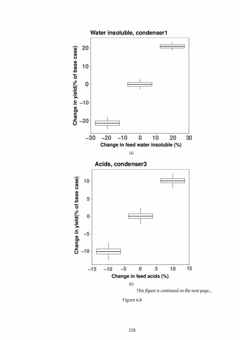
(a)

(b)

This figure is continued on the next page...

Figure 6.8

228

(c)

(d)

This figure is continued on the next page...

Figure 6.8

229

(e)

(f)

This figure is continued on the next page...

Figure 6.8

230

(g)

Figure 6.8: Sensitivity study of concentration of model compounds used to repre-sent bio-oil.

6.3.2 Pyrolysis vapor fractionation

6.3.2.1 Fractional condensation of pyrolysis vapors: Scheme 1

A train of indirect contact heat exchangers is the most simple and widely used

configuration for stage-wise condensation of pyrolysis vapors. The separation of

chemical families is governed by the boiling point and mole fractions of compo-

nents in the vapor mixture. The simulations predict that phase separation occurs

at temperatures below 160◦C, 70◦C and 60◦C for first, second and third stage re-

spectively. For the third stage proportion of one of the phase (signified as Liq1-3-1)

is very less and can be ignored. Figure 6.9 shows the degree of separation achieved

between chemical families for the operating conditions shown in Table 6.3.

231

(a)

(b)

This figure is continued on the next page...

Figure 6.9

232

(c)

(d)

This figure is continued on the next page...

Figure 6.9

233

(e)

(f)

This figure is continued on the next page...

Figure 6.9

234

(g)

(h)

This figure is continued on the next page...

Figure 6.9

235

(i)

Figure 6.9: Separation factors of chemical families in different liquid streams ob-tained for scheme 1

Figure 6.9 illustrates the separation factor for liquid 1-2-1. Chemical families (CF)

1-1, 1-2 and 2 are condensed together in the first condenser. The separation factor

SF(1−2)−1 is close to 0.99 in the first stage below 200◦C but SF(1−1)−1 and SF2−1

is also 0.43 and 0.37 respectively. The phase separation does not result in any sig-

nificant fractionation between CF1-1 and CF1-2, despite their chemically different

nature. The absence of water, due to high condenser temperature, from Liq1-1-1

prevents the phase separation of CF1-1 from CF1-2. A temperature of 170 ◦C was

optimized for stage one to maximize separation between CF1-1 and CF-2 as they

have similar nature and can pose difficulty in downstream purification. At 170◦C,

values of SF(1−1)−1 and SF(1−2)−1 reached a maximum, while separation factors

for all other chemical families were atminimum. The optimal temperature condi-

tion for stage 2 is 90◦C, where remaining CF1-1 is recovered completely while CF3

and CF4 yields areminimized. The temperature of third and fourth condenser are

optimized to 50 and -5◦C respectively to maximize the separation between CF3

and CF4, and maximize the overall recovery of bio-oil.

236

Table 6.4: Liquid yield and purity of components for scheme 1 under optimizedoperating conditions for NCG: condensible ratio of 2.87

Liquid Yield (Purity), wt.%

Components MW bp (◦C) Cond 1 Cond 2 Cond 3 Cond 4

Water 18.02 100 0.15 (0.14) 2.88 (3.02) 71.38 (67.4) 23.07 (79.94)

Formic Acid 46.02 101 0.4 (0) 3.17 (0.03) 73.17 (0.59) 21.58 (0.64)

Acetic Acid 60.05 118 0.67 (0.17) 13.94 (4.07) 71.18 (18.73) 13.43 (12.97)

Propionic acid 74.08 141 0.98 (0.05) 20.61 (1.17) 64.57 (3.29) 13.01 (2.43)

Acetol 74.08 145 0.91 (0.04) 42.51 (2.07) 53 (2.32) 3.51 (0.57)

Glyoxal 58.04 51 0.07 (0) 0.82 (0.03) 6.92 (0.25) 9.35 (1.22)

Glycol aldehyde 60.05 131 1.15 (0.04) 61.78 (2.44) 36.2 (1.29) 0.86 (0.11)

Gamma Butyrolactone 86.09 204 3.34 (0.41) 73.71 (10.38) 20.1 (2.55) 2.67 (1.24)

Furfural 96.08 161 0.87 (0.01) 38.52 (0.46) 40.86 (0.44) 18.24 (0.72)

Furfuryl alcohol 98.10 171 1.02 (0.01) 57.53 (0.69) 38.24 (0.41) 3.15 (0.12)

o-Cresol 108.14 191 63.04 (3.58) 35.94 (2.32) 1.02 (0.06) 0 (0)

p-Cresol 108.14 202 70.83 (4.02) 27.68 (1.78) 1.47 (0.09) 0.02 (0)

2,4-Xylenol 122.16 210 61.31 (5.14) 37.5 (3.57) 1.19 (0.1) 0.01 (0)

Guaiacol 124.14 205 2.46 (0.13) 81.31 (4.76) 16.2 (0.86) 0.03 (0.01)

4-methyl Guaiacol 138.16 221 2.66 (0.04) 90.42 (1.41) 6.92 (0.1) 0.01 (0)

iso-Eugenol 164.20 266 9.26 (0.2) 90.14 (2.24) 0.59 (0.01) 0 (0)

Vanillin 152.15 285 25.41 (0.28) 74.45 (0.93) 0.14 (0) 0 (0)

Syringol 154.16 261 7.09 (0.42) 92 (6.23) 0.91 (0.06) 0 (0)

1,2-Benzenediol 110.10 245 36.61 (1.09) 61.66 (2.08) 1.73 (0.05) 0 (0)

trans-3,5-dimethoxystilbene 240.30 375 81.11 (10.66) 18.89 (2.82) 0 (0) 0 (0)

1,2-diphenyl ethane 182.26 284 2.49 (0.55) 92.71 (23.39) 4.51 (1.02) 0.02 (0.01)

diBenzofuran 168.19 285 11.3 (2.36) 86.88 (20.59) 1.8 (0.38) 0.01 (0.01)

High

molecular weight lignin-2406.43 634 100 (9.09) 0 (0) 0 (0) 0 (0)

High

molecular weight lignin-1394.42 648 100 (9.09) 0 (0) 0 (0) 0 (0)

Xylose 150.13 96.77 (9.05) 3.23 (0.34) 0 (0) 0 (0)

Levoglucosan 162.14 99.45 (21.47) 0.55 (0.13) 0 (0) 0 (0)

Cellobiose 342.30 100 (20.18) 0 (0) 0 (0) 0 (0)

Dehydroabietic acid 300.44 39.89 (1.78) 60.1 (3.05) 0.01 (0) 0 (0)

237

Table 6.4 shows yield and purity of each compound obtained under optimal oper-

ating conditions for scheme1. Compounds like guaiacol, syringol and 1,2- diphenyl

ethane that havemole fractions andboilingpoints similar to or greater than cresols

and xylenol did not condense significantly in stage 1. When stage 1 condenser

is simulated at 260◦C, 14 wt.% (based on feed) of o- and p-cresol, and 10 wt.%

of 2,4-xylenol condense despite condenser temperature being higher than their

respective boiling points. Such a anomalous behavior is corroborated by GC-MS

profile of fractionally condensed bio-oil reported in [19]. To analyze which com-

pounds strongly interact with cresols and xylenol and cause them to condense at

high temperature, the flow rate of eachmodel component is equaled to zero one at

a time, while keeping the flow rate of other components constant. For example,

in one instance the water flow rate is equaled to zero and flow rate of all other

components is calculated based on mass fractions from Table 6.1. The mass ra-

tio of non-condensible to condensible components is maintained at 2.87 for each

case and optimal temperature conditions are used for the condensers. As mole

fraction in liquid or vapor phase is an actual measure of driving force for mass

transfer, the ratio of volatility of a component under altered feed conditions to

its volatility for the base case (where feed conditions are as stated in Table 6.1)

is plotted as points in Figure 6.10. On the other hand the percent change in the

mass yield of each component is shown as bar chart for an easier comprehension

of co-condensation effect.

238

(a)

(b)

This figure is continued on the next page...

Figure 6.10

239

(c)

Figure 6.10: Relative volatility dependence of model components

Compounds that have significantly condensed at each stage are plotted in Figure

6.10. Effect of water on condensation is also tested because, following nitrogen,

water has the highest mole fraction in the pyrolysis vapor stream and thus, pro-

foundly affects the dew point of the vapor mixture. Condensation of the com-

pounds represented by marker shape (group 1) is affected by absence of com-

pounds indicated by color (group 2) in the figure legend. Though high and low

molecular weight phenols are present in stage 1, they do not affect the conden-

sation or co-condensation of other components significantly. The mass yield and

volatility of cresols and xylenol in stage 1 is significantly affected by levoglucosan

and cellobiose as compared to xylose and water (Figure 6.10 (a)). The yield of

cresols and xylenol decreases to an average value of 69±3 wt.% (on the basis of

mass yield for base case) when levoglucosan and cellobiose are absent in the feed,

since the bubble point of the mixture decreases in the absence of sugars. On the

other hand relative volatility of benzenediol does not change but the yield de-

creases to 81±4 wt.% in the absence of sugars and increases to 131 wt.% in the

absence of water. Yield of iso-eugenol (mole fraction comparable to benzenediol)

240

and diphenylethane (mole fraction 10 times of benzenediol) increases in the ab-

sence of sugars. To generalize, points that lie in the second quadrant indicate

that yield decreases as a result of decrease in the bubble point of the mixture as

a consequence of absence of high boiling compounds. On the other hand, points

in the fourth quadrant imply a weak interaction amongst group 1 and group 2

compounds.

For condenser 2, most of the points are clustered around the origin which show

that, at operating condition of 70◦C, the composition of the condensate is not con-

siderably sensitive to feed composition. Points lying in the third quadrant, where

relative volatility and yield both decrease, suggest the effect of upstream con-

denser. The points correspond to o- and p-cresol when xylenol is not present in

the feed. The absence of xylenol causes an increase in the yield of cresols (122

wt.%) and a decrease in relative volatility ( 0.45). Similarly if any point lies in

the first quadrant, the yield and relative volatility of corresponding group 1 com-

pound(s) would have decreased and increased respectively under the influence of

group 2 component. Similar behavior is observed for components condensing in

stage 3.

Thus, to sumup, condensation of phenols is strongly affected by sugars in the first

condenser. The effect of components on the each other’s condensation becomes

less prominent after the first stage because the operating temperatures are well

below the boiling point of most of the components. The amount of inert/carrier

gas used in the fast pyrolysis reaction depends on the reactor configuration. For

example the amount of carrier gas used in a bubbling fluidized bed reactor ismore

as compared to that used in an auger reactor. Thus, the effect of amount of non-

condensible gas on the operating conditions and bio-oil condensation is studied.

As the NCG: condensible ratio decreases, higher condenser temperatures are re-

quired to achieve a similar extent of separation between chemical families. The

optimal conditions of condensers, yield, and purity of chemical families are pre-

sented in Figure 6.11. Also, there is no significant difference between the yield of

individual chemical compounds obtained under optimal operating conditions for

each of the case in Figure 6.11.

241

Figure6.11:Scheme1yieldandpurityofchemicalfamiliesunderoptimaloperatingconditionsfordifferentmassratiosofNCG:condensible

components

242

On the other hand, when the operating conditions are kept constant and the NCG

ratio is varied (Table 6.5), yields of components having boiling points less than

132◦C (acetol) are affected significantly. The saturation temperature vs. satura-

tion pressure curves are exponential in nature [18] and if the saturation pressure

falls below a limit, a small change in saturation pressure, the saturation tempera-

ture decreases drastically. Therefore, the yield ofwater, acids and acetol decreases

in condenser 3 for NCG: condensible ratio of 2.87. However, yield of compounds

like cresols in the first condenser is not significantly different, again proving that

there is a strong interaction between cresols and chemical family 1-1 and 1-2.

6.3.2.2 Fractional condensation of pyrolysis vapors: Scheme 2

Increase in the non-condensible gas content improves the separation ability be-

tween chemical families. However, increasing the non-condesible gas content

would increase the cooling duty. Therefore, for scheme2, indirect contact heat ex-

changers were replaced with spray towers using water as a cooling medium. The

flow rate and temperature of cooling water was maintained so that water evap-

orated completely, cooling the pyrolysis vapors in the two spray towers. Evap-

orated water decreases the bubble point of the vapor exiting the spray towers.

The vapor and liquid streams exiting the spray towers have different tempera-

tures. The different liquid and vapor temperatures, along with the increase in

mole fraction of water in the vapor phase improves the separation ability of the

chemical families.

The conditions for scheme 2were optimized using the separation factors of chem-

ical families as done for scheme1. Figure 6.12 shows the effect ofNCG: condensible

ratio on the separability of bio-oil components along with the optimal conditions

for each case. The yield and purity of the chemical families represented in the

figure is on water-free basis. Direct contact counter-current cooling in the tower

resembled a stripping section of distillation column, where, downward moving

liquid, formed at the top of the spray tower, was reheated by the pyrolysis gas

traveling upwards. The reheating led to evaporation of some low boiling compo-

nents and condensation of high boiling components from the vapor.

243

Table 6.5: Effect of NCG: Condensible mass ratio on yield of each bio-oil modelcomponent

Scheme 1

Component Yield (wt.%) for NCG: Condensibles mass ratio 1.5 Yield (wt.%) for NCG: Condensibles mass ratio 2.87

Cond 1

(190◦C)

Cond 2

(110◦C)

Cond 3

(60◦C)

Cond 4

(-5◦C)

Cond 1

(190◦C)

Cond 2

(110◦C)

Cond 3

(60◦C)

Cond 4

(-5◦C)

Water 0.15 0.42 29.21 0.08 68.83 0.09 0.23 2.44 3.91 90.87

Formic Acid 0.43 0.71 33.06 0.22 64.73 0.25 0.37 3.48 2.30 91.95

Acetic Acid 0.64 2.77 52.07 1.05 43.05 0.37 1.53 13.46 5.65 77.88

Propionic acid 0.89 4.37 52.41 1.88 40.03 0.51 2.42 19.38 5.23 71.40

Acetol 0.83 8.25 71.51 0.86 18.49 0.45 4.18 44.95 8.69 41.57

Glyoxal 0.08 0.23 2.98 0.07 38.86 0.04 0.12 0.67 0.36 32.89

Glycol aldehyde 0.97 11.52 76.85 0.99 9.66 0.52 6.11 45.37 25.93 22.05

Gamma

Butyrolactone3.00 34.72 39.25 10.54 12.37 1.63 21.40 52.79 4.87 19.11

Furfural 0.82 9.12 37.22 6.73 45.51 0.44 4.74 35.56 5.35 53.07

Furfuryl alcohol 0.94 15.84 55.86 9.00 18.30 0.51 8.63 48.52 7.31 34.89

o-Cresol 58.71 17.06 24.23 0.00 0.00 52.42 14.63 1.32 31.63 0.00

p-Cresol 66.17 18.79 13.72 1.04 0.29 59.98 17.40 21.20 0.80 0.60

2,4-Xylenol 56.46 27.02 14.54 1.71 0.27 48.59 24.95 25.69 0.45 0.32

Guaiacol 2.26 27.42 68.04 1.17 1.11 1.24 15.68 62.98 13.03 7.07

4-methyl Guaiacol 2.24 47.57 48.17 1.60 0.41 1.16 30.97 57.89 7.54 2.43

iso-Eugenol 7.29 83.08 8.62 0.99 0.02 3.84 76.93 17.94 1.23 0.07

Vanillin 18.93 76.00 5.05 0.02 0.00 11.24 77.62 8.22 2.91 0.01

Syringol 5.47 76.64 17.74 0.14 0.01 2.90 64.46 24.62 7.91 0.10

1,2-Benzenediol 32.11 46.51 21.33 0.04 0.01 22.08 41.21 27.69 8.69 0.33

trans-3,5-

dimethoxystilbene70.02 29.97 0.00 0.01 0.00 53.65 46.29 0.05 0.00 0.00

1,2-diphenyl ethane 1.95 71.44 0.43 24.49 0.52 0.97 56.75 39.05 0.18 1.28

diBenzofuran 9.72 74.83 10.28 4.96 0.22 5.46 66.29 26.48 1.25 0.52

High molecular

weight lignin-2100.00 0.00 0.00 0.00 0.00 100.00 0.00 0.00 0.00 0.00

High molecular

weight lignin-1100.00 0.00 0.00 0.00 0.00 100.00 0.00 0.00 0.00 0.00

Xylose 93.19 6.81 0.00 0.00 0.00 87.38 12.61 0.00 0.01 0.00

Levoglucosan 98.58 1.42 0.00 0.00 0.00 97.19 2.81 0.00 0.00 0.00

Cellobiose 100.00 0.00 0.00 0.00 0.00 100.00 0.00 0.00 0.00 0.00

Dehydroabietic acid 27.85 71.95 0.00 0.19 0.00 15.79 83.72 0.49 0.00 0.00

244

Figure6.12:Scheme2yieldandpurityofchemicalfamiliesunderoptimaloperatingconditions

245

For an NCG: condensible ratio of 2.87, the liquid stream from the first condenser

exited at 250◦C and the vapor stream at 144◦C. The low temperature at the top of

the tower was a result of water evaporation which caused condensation of chem-

ical family 1-1 and 1-2 components. As the liquid descended along the column,

it was stripped of chemical family 2 components (except alkyl phenols). For con-

denser 2, liquid stream exited at 96◦C and vapor at 74◦C. The liquid in second con-

denser was stripped of chemical family 3, which was present in significant quan-

tities in condenser 2 for scheme 1. Figure 6.13 shows the distribution of chemical

functionalities in different condensers for scheme 1 and scheme 2. Thus, the use

of direct contact heat exchanger improves the separation amongst the chemical

families as compared to indirect contact heat exchangers.

246

(a)

(b)

Figure 6.13: Comparison of scheme 1 and scheme 2 for chemical family yields ineach condenser.

247

To test if coolingmediumhas any effect on the selective condensation of any com-

ponent, water was replaced by toluene. Toluene flow rate and temperature were

adjusted so that temperature of the liquid and vapor stream exiting the column

were same when water was used as a cooling medium. Toluene did not have any

effect on the selective condensation of any component in condenser 1. However,

in condenser 2, the yield of propionic acid, butyrolactone, furfural, furfuryl al-

cohol and 1,2-diphenylethane increased approximately 2.2±0.7 folds while that

of acetol and glycoldehyde decreased by 0.6±0.05 fold. Compared to pyrolysis

oil components, significant amount of toluene was condensed in stage 2 which

therefore, affected condensation selectivity of several compounds. Thus, in case

of a direct contact heat exchanger, the liquid and vapor composition is affected by

their respective exit temperatures. If the coolingmedium condenses, it can affect

the distribution of compounds in the vapor and liquid phase.

The energy required to condense 1 kg of bio-oil (onwater free basis), using scheme

1, for NCG: condensible ratio of 2.87, 2.5 and 1.5 was 5.91, 5.59, and 4.65MJ/kg-bio-

oil respectively. Using scheme 2 the energy requirement for NCG: condensible ra-

tio of 2.87, 2 and 1.5 was 5.93, 5.15, and 4.71 MJ/kg-bio-oil respectively. Energy

required to cool the liquid to 25◦C was also considered for calculation. The en-

ergy consumption increases linearly with respect to non-condensible gas content

but there is no significant difference between energy requirement between two

schemes. Though scheme 2 improves the separability between chemical families,

but, the water content in the third and fourth stage increases, which can make

recovery of acids and carbonyl compounds energy intensive.

248

Table 6.6: Liquid yield and purity of components for scheme 2 under optimizedoperating conditions for NCG: condensible ratio of 2.87

Liquid Yield (Purity), wt.%

Components Cond 1 Cond 2 Cond 3 Cond 4

Formic Acid 0.09(0) 0.96(0.01) 54.09(1.45) 0.02(0) 44.25(2.08)

Acetic Acid 0.1(0.03) 4.5(1.54) 63.45(55.69) 0.18(0.75) 31.54(48.44)

Propionic acid 0.13(0.01) 6.84(0.45) 56.59(9.62) 0.41(0.34) 35.71(10.62)

Acetol 0.11(0) 28.37(1.62) 56.58(8.28) 0.08(0.06) 14.81(3.79)

Glyoxal 0.02(0) 0.31(0.01) 3.99(0.47) 0.01(0.01) 37.4(7.76)

Glycol aldehyde 0.12(0) 45.85(2.12) 48.04(5.7) 0.07(0.04) 5.91(1.23)

Gamma Butyrolactone 0.55(0.07) 52.42(8.65) 23.64(10.01) 4.92(10.12) 18.2(13.48)

Furfural 0.14(0) 12.75(0.18) 19.22(0.69) 2.28(0.4) 64.47(4.06)

Furfuryl alcohol 0.17(0) 25.68(0.36) 47.81(1.72) 3.32(0.58) 22.93(1.45)

o-Cresol 41.06(2.43) 58.9(4.45) 0.03(0.01) 0(0) 0(0)

p-Cresol 54.82(3.24) 39.3(2.97) 4.25(0.82) 0.49(0.46) 1.14(0.39)

2,4-Xylenol 48.63(4.25) 45.53(5.08) 3.92(1.12) 0.75(1.04) 1.16(0.58)

Guaiacol 0.49(0.03) 80.88(5.55) 17.59(3.1) 0.11(0.09) 0.93(0.29)

4-methyl Guaiacol 0.59(0.01) 93.17(1.7) 5.76(0.27) 0.15(0.03) 0.33(0.03)

iso-Eugenol 4.72(0.11) 95.08(2.76) 0.14(0.01) 0.02(0.01) 0(0)

Vanillin 9.07(0.1) 90.9(1.33) 0(0) 0(0) 0(0)

Syringol 1.76(0.11) 98.18(7.79) 0.05(0.01) 0(0) 0(0)

1,2-Benzenediol 11.77(0.36) 88.11(3.48) 0.11(0.01) 0(0) 0(0)

trans-3,5-dimethoxystilbene 94.82(12.98) 3.89(0.68) 0(0) 0(0) 0(0)

1,2-diphenyl ethane 0.58(0.13) 72.53(21.45) 0.01(0) 22.6(83.36) 4.26(5.65)

diBenzofuran 5.04(1.1) 92.59(25.72) 1.44(1.02) 0.78(2.69) 0.13(0.16)

High

molecular weight lignin-299.16(9.39) 0(0) 0(0) 0(0) 0(0)

High

molecular weight lignin-199.9(9.46) 0(0) 0(0) 0(0) 0(0)

Xylose 98.76(9.63) 1.19(0.15) 0(0) 0(0) 0(0)

Levoglucosan 99.93(22.48) 0.05(0.01) 0(0) 0(0) 0(0)

Cellobiose 100(21.02) 0(0) 0(0) 0(0) 0(0)

Dehydroabietic acid 65.83(3.06) 32.23(1.92) 0(0) 0.02(0.01) 0(0)

249

6.4 Summary

Biomass pyrolysis oil is a complex mixture of hundreds of chemical compounds,

that pose a difficulty in simulating bio-oil separation processes. Therefore, bio-

oil composition was represented using twenty-eight model compounds based on

their abundance in bio-oil. The model compounds were classified into five chem-

ical families. As the compounds are polar in nature it was important to test the

accuracy of the phase equilibrium model used in simulations. Therefore, a liter-

ature reported multistage bio-oil collection system was simulated initially. The

error between the experimental and predicted values for liquid phase composi-

tion of various chemical families in different liquid streams using NRTL-NTH and

UNIQUAC-NTH phase equilibrium models was 8.86±11.05% and 9.90±12.38% re-

spectively. Further, variation of binary interaction parameters within a range of

±40% did not have a significant effect on the prediction ability of liquid compo-

sition. Thus, UNIQUAC and NRTL activity coefficient models coupled with NTH

equation of state can be used to design bio-oil fractionation or collection systems

with a fair degree of accuracy.

To address the bio-oil stability issue, two different condensation schemes were

simulated to separate constituent chemical families from one another. A train

of four indirect contact heat exchangers was simulated over a wide range of op-

erating conditions with an objective to separate the chemical families from one

another. Such a simplified and widely used bio-oil recovery approach was found

unsuitable for fractionation of chemical families. Therefore, first two heat ex-

changers were replaced by direct contact cooling towers, where water was used

as the cooling medium. The direct contact heat exchangers were similar to the

stripping section of a distillation column. This led to increase in the recovery of

phenols in the first two condensers while acids, aldehydes, ketones and furfurals

condensed in stage 3 and stage 4. Moreover, the energy requirement for both the

schemes is the same. However, water content significantly increases in the liquid

streams obtained from third and fourth stage, which canmake recovery of organic

components energy intensive. Also the modified condensation scheme could not

effectively separate chemical family 3 and 4 from one another.

250

Chapter 7

Closure and future work

7.1 Closure

The present research focused onmodeling and simulation of different biomass py-

rolysis phenomena that occur over a wide range of length and time scales. Reac-

tion kinetics and first principle bubbling fluidized bed reactor (BBR)models along

with simulation strategies for pyrolysis vapor condensation were developed to

understand various aspects of upstream and downstream operations in biomass

pyrolysis process. Experiments were carried out to understand andmodel weight

loss kinetics of biomass under a wide range of pyrolysis conditions.

Yield and composition of pyrolysis products exiting a BBR depend on rate of py-

rolysis reaction which in turn depends on operating temperature, heat and mass

transfer rates, and residence time of solid and vapor phases. Further, bio-oil sta-

bility depends on liquid collection system succeeding the pyrolysis reactor. To un-

derstand the multi-scale nature and complex interaction between different pro-

cesses in biomass pyrolysis a multi-layered approach was adopted.

Based on experimental findings of presentwork amulti-reaction single step kinet-

ics was developed using distributed activation energy (DAE) approach. Literature

studies limit themselves to using a narrow range of heating rate and particle sizes

to determine kinetic parameters. Therefore, a systematic study was performed to

study the effect of heating rate and particle size on the rate of pyrolysis reaction.

Further, the findings of these experiments along with other literature reports

were used to develop a detailed lumped kinetic model using DAE approach. The

251

detailed lumped model is capable of predicting the composition of major bio-oil

and gas components as against a lumpedmodel which gives global vapor and solid

yields. At reactor scale different hydrodynamic parameters affect the reactor’s

performance (gas, liquid, and solid yield and composition). Mixing characteris-

tics of a reactor influence the gas-solid heat andmass transfer coefficients, which

affect the selectivity of devolatilization and char forming reactions in biomass

particle. Also, long gas residence time leads to secondary reactions reducing the

liquid yield. An extensible 1-D BBR reactor model was developed to assess the

performance of kinetics developed in the present study. The reactor model uses

a rigorous secondary reaction mechanism to simulate gas the phase reactions of

biomass pyrolysis. The reactor scale model gives global yields of gas, liquid, and

solid products along with composition of liquid and gas products. Based on the

major components of bio-oil, liquid collection schemes were simulated to frac-

tionally condense bio-oil into distinct chemical families. The simulations were

carried out over a wide range of operating conditions. Sensitivity analysis of feed

composition was conducted to understand its effect on condensation behavior of

different chemical families. Following paragraphs describe the outcomes of the

present work in these three areas of biomass pyrolysis.

1. Experimental findings of biomass (Mallee wood and bark) pyrolysis

(a) Studied the effect of heating rate on changes inmorphologyof biomass

particle.

(b) Increase in heating rate caused the biomass particle to soften and led

to formation of bubbles on the particle surface.

(c) Thepartialmelting is attributed to increase in selectivity for deploymer-

ization reactions over char forming reactions.

(d) Morphological changes that occur beyond heating rate of 75◦C/min,

affect the rate of biomass volatilization.

(e) The uneven shift in the mass loss profile of biomass is attributed to

changes in the pores structure of biomass particle.

(f) The study demonstrates that the choice of heating rate to determine

biomass pyrolysis reaction kinetics is vital.

252

2. Kinetic modeling of biomass pyrolysis

(a) Developed a multi-reaction single step and detailed lumped kinetic

model based on the DAE approach.

(b) For heating rates where softening or partial melting of biomass par-

ticle was dominant, an increase in the frequency factor was observed

for the single step lumped model.

(c) This finding led to incorporation of correction factor dependent on

heating rate for the detailed lumped model.

(d) The effect of qualitatively observedmorphological changeswere trans-

lated quantitatively in the reaction kinetics using the correction fac-

tor.

(e) Coupling of detailed lumped kinetic model and DAE approach caused

substantial improvement in prediction of biomass pyrolysis reaction

rate.

(f) DAE coupled detailed lumped model also incorporates prediction of

additional monomeric lignin components.

Chapter 3 outlines the impact of heating rate and particle size on biomass

morphology, pyrolysis kinetics, and highlights the importance of selection

of experimental conditions on kinetic model parameters. The results show

that extrapolation of TGA derived kinetics to large scale fast pyrolysis re-

actors is feasible if TGA experiments are carried out such that biomass par-

ticles (correctly representing length scale of pore structure) experiences

similar conditions as those within the reactor. Compared to slow pyroly-

sis the reaction selectivity and physical changes in biomass particles are

completely different under fast pyrolysis conditions. The plasticity elicited

in biomass particles undergoing pyrolysis can be used as an indicator for

increased selectivity of depolymerization and volatilization reactions over

cross-linking/ char forming reactions. Moreover, partial melting or soften-

ing of biomass particle, observed under fast pyrolysis conditions, increases

molecularmobility and also causes bubble formation, which results in open

pore structure. Significant plasticity was induced in biomass particles at

253

heating rates of 200 and 250 ◦C/min. It implies that kinetic parameters de-

rived using the mass loss data obtained at these heating rates could be ex-

trapolated to fast pyrolysis. The DAEM is valid over a wide range of heating

rates and it is also capable of quantifying the effect of molecular hetero-

geneity in solids and in-situ physical changes on pyrolysis reaction kinetics

using a probabilistic distribution of activation energy.

Chapter 4 couples the DAE modeling strategy with literature reported de-

tailed pyrolysis kinetics. The coupling extends the applicability of model

to wide range of heating rates and takes into account the effect of biomass

plasticity on reaction rates. As ash has a significant effect on biomass plas-

ticity and reaction selectivity, themodel parameters are derived for biomass

with ash content < 1 and > 1 wt.%. The model additionally highlights that

biomass undergoes considerablemass loss as its temperature rises to the re-

actor temperature. Thus, the consideration ofmass loss in dynamic temper-

ature is important to determine accurate kinetic parameters. This justifies

the employment of TGA for determining the pyrolysis kinetic parameters.

3. Reaction engineering model of bubbling fluidized bed reactor for biomass

pyrolysis

(a) Developed an extensible reaction engineering model of bubbling flu-

idized bed reactor using a mixing cell framework.

(b) The BBR model was used to simulate biomass pyrolysis using rigor-

ous primary (developed in the present study) and secondary reaction

kinetics.

(c) TheDAE coupleddetailed lumpedmodel performsbetter than themodel

reported in literature when global yields of gas, liquid, and solid prod-

ucts were compared.

Chapter 5 tests the primary reaction kinetic model developed in Chapter 4

and compares its performance with that reported in the literature at the

reactor scale. The improved kinetic model performs better than the one in

the literature at all, especially low, temperatures. Thus, considering pyrol-

ysis behavior of biomass particles while they experience temperature rise

254

in the reactor is vital for determining kinetic model parameters. Also, the

results show that consideration of DAEM to account for the effect of plastic-

ity on reaction rate is vital for accurate prediction of yield and composition

of pyrolysis liquid, gas, and solid. The reactor model, with certain mod-

ifications, can be used to design large scale pyrolysis reactors capable of

handling different kinds of biomass.

4. Fractional condensation of biomass pyrolysis vapors

(a) Simulated pyrolysis vapor condensation schemes over a wide range of

operating conditions using representative model compounds.

(b) A literature reportedmultistage bio-oil collection systemwas initially

simulated to test the accuracy of the phase equilibriummodel used in

simulations. Predictions using UNIQUAC-NTH and NRTL-NTH models

showed good agreement with the literature experiments.

(c) The simulation strategy can be used to design collection systems for

biomass pyrolysis vapors.

(d) A train of standard indirect contact heat exchangers was found un-

suitable for fractionation of chemical families.

(e) Use of water spray towers instead of indirect contact heat exchangers

resulted in effective separation of phenols fromaldehydes andketones

(most reactive components of bio-oil) without substantial increment

in the energy requirement.

Chapter 6 proposes simulation strategy to design downstream unit opera-

tions for pyrolysis plants and a scheme to fractionally condense pyrolysis

vapors into distinct chemical families. The simulation strategy can be ex-

tended to pyrolysis vapors of different composition and the condensation

scheme can be designed accordingly.

Commercial success of biomass fast pyrolysis process is hinderedbyvariable biomass

composition, the complex nature of pyrolysis chemistry, and bio-oil instability.

Accurate modeling of reaction kinetics and determination of parameters is vital

for reactor design. The thesis reports models for reaction kinetics, reactor, and

255

condensation systems. These multi-scale models can be coupled to design fast

pyrolysis plants that use completely different biomass varieties to get bio-oil.

This research has helped understand various complex phenomena, which span

over a wide range of length and time scales, of biomass pyrolysis process. How-

ever, there still persist many issues.

7.2 Future work

The effect of heating rate on biomass pyrolysis needs further exploration. Only

one biomass type was used in this study. Morphological changes in biomass par-

ticle not only depend on heating rate but also on the biomass composition - cel-

lulose, hemicellulose, lignin, and ash content. It will be interesting to determine

the range of heating rate where morphological changes become significant for

different biomass species. This may serve as a guide to define a new, composi-

tion dependent, variable to account for the effect of morphological changes on

pyrolysis reaction kinetics. The effect of various ash constituents on distribution

of biomass pyrolysis products needs to be incorporated in the reaction kinetics.

Further, the detailed lumped kinetic model needs to be validated using detailed

bio-oil composition. Adding more reactions to the detailed kinetic model using

results frommolecular simulations of cellulose, hemicellulose, and lignin pyroly-

sis may improve the prediction ability of bio-oil components.

The reactor model has been applied to a small pilot scale reactor. To improve its

predictability computational fluid dynamics (CFD) can be used to accurately esti-

mate the velocity profiles and volume fractions of different phases in the reactor.

As biomass reacts, its physical properties change and so does its mixing behavior.

Itwill be interesting to developnewcorrelations for estimating thehydrodynamic

parameters for biomass pyrolysis reactors by simulating several reactor geome-

tries using Lagrangian approach. Further, the reactor model can be coupled with

a single particle model to extend the range of biomass particle size the model can

handle.

Fractional condensation of pyrolysis vapors into distinct chemical families has po-

tential to add value to bio-oil. Bio-oil is a complex liquid with organic and aque-

256

ous phases, which undergo separation depending on the composition of bio-oil.

Moreover, high molecular weight tar compounds form a large fraction of bio-oil

whose structure is not defined accurately. Thermodynamics of phase equilibrium

for bio-oil is complex. Accurate experimentation to study the condensation be-

havior of bio-oil model compounds in the presence of one another is essential.

Rigorous experimental validation of simulations will thus, help establish a robust

strategy for designing downstream operations for commercial pyrolysis plants.

257

Appendix A

A.1 Appendix: Chapter 3

A.1.1 Experimental data

258

(a)

(b)

This figure is continued on the next page...

Figure A.1

259

(a)

(b)

This figure is continued on the next page...

Figure A.1

260

(c)

(d)

This figure is continued on the next page...

Figure A.1

261

(e)

Figure A.1: Experimental values of α for biomass particle size less than 45 µm

262

(f)

(g)

This figure is continued on the next page...

Figure A.2

263

(a)

(b)

This figure is continued on the next page...

Figure A.2

264

(c)

(d)

This figure is continued on the next page...

Figure A.2

265

(e)

Figure A.2: Experimental values of dα/dt for biomass particle size less than 45 µm

266

(f)

(g)

This figure is continued on the next page...

Figure A.3

267

(a)

(b)

This figure is continued on the next page...

Figure A.3

268

(c)

(d)

This figure is continued on the next page...

Figure A.3

269

(e)

Figure A.3: Experimental values of α for biomass particle size between 75 to 106µm

270

(f)

(g)

This figure is continued on the next page...

Figure A.4

271

(a)

(b)

This figure is continued on the next page...

Figure A.4

272

(c)

(d)

This figure is continued on the next page...

Figure A.4

273

(e)

Figure A.4: Experimental values of dα/dt for biomass particle size between 75 to106 µm

274

(f)

(g)

This figure is continued on the next page...

Figure A.5

275

(a)

(b)

This figure is continued on the next page...

Figure A.5

276

(c)

(d)

This figure is continued on the next page...

Figure A.5

277

(e)

Figure A.5: Experimental values of α for biomass particle size between 300 to 425µm

278

(f)

(g)

This figure is continued on the next page...

Figure A.6

279

(a)

(b)

This figure is continued on the next page...

Figure A.6

280

(c)

(d)

This figure is continued on the next page...

Figure A.6

281

(e)

Figure A.6: Experimental values of dα/dt for biomass particle size between 300 to425 µm

282

Appendix B

B.1 Appendix: Chapter 6

283

TableB.1:Yieldandpurityofbio-oilmodelcomponentsforscheme1fordifferentNCG:condensiblemassratio.

NCG:Condensiblemassratio1.5

Liquidyield(purity),wt.%

NCG:Condensiblemassratio2

Liquidyield(purity),wt.%

Components

Cond1

Cond2

Cond3

Cond4

Cond1

Cond2

Cond3

Cond4

FormicAcid

0.15

(0.15)

0.42

(0.63)

29.21

(40.46)

0.08

(0.85)

68.83

(77.42)

0.13

(0.13)

0.41

(0.59)

0.09

(0.96)

32.81

(43.34)

64.39

(78.13)

AceticAcid

0.43 (0)

0.71

(0.01)

33.06

(0.39)

0.22

(0.02)

64.73

(0.62)

0.35 (0)

0.63

(0.01)

0.21

(0.02)

35.44

(0.4)

61.9

(0.64)

Propionicacid

0.64

(0.17)

2.77

(1.17)

52.07

(20.1)

1.05

(3.08)

43.05

(13.49)

0.56

(0.15)

2.77

(1.13)

1.06

(3.29)

55.08

(20.27)

39.83

(13.47)

Acetol

0.89

(0.05)

4.37

(0.36)

52.41

(3.92)

1.88

(1.06)

40.03

(2.43)

0.79

(0.04)

4.45

(0.35)

1.94

(1.16)

55

(3.92)

37.12

(2.43)

Glyoxal

0.83

(0.04)

8.25

(0.58)

71.51

(4.6)

0.86

(0.42)

18.49

(0.97)

0.73

(0.03)

8.82

(0.6)

1.08

(0.56)

72.8

(4.47)

16.48

(0.93)

Glycolaldehyde

0.08 (0)

0.23

(0.01)

2.98

(0.16)

0.07

(0.03)

38.86

(1.65)

0.06 (0)

0.21

(0.01)

0.07

(0.03)

2.87

(0.14)

26.28

(1.2)

284

TableB.1continuedfrom

previouspage

NCG:Condensiblemassratio1.5

Liquidyield(purity),wt.%

NCG:Condensiblemassratio2

Liquidyield(purity),wt.%

Components

Cond1

Cond2

Cond3

Cond4

Cond1

Cond2

Cond3

Cond4

Gamma-Butyrolactone

0.97

(0.04)

11.52

(0.65)

76.85

(4.01)

0.99

(0.39)

9.66

(0.41)

0.88

(0.03)

13.22

(0.73)

1.22

(0.51)

77.13

(3.84)

7.53

(0.34)

Furfural

3

(0.39)

34.72

(7.04)

39.25

(7.31)

10.54

(14.87)

12.37

(1.87)

2.66

(0.34)

36.39

(7.17)

10.98

(16.37)

38.5

(6.83)

11.26

(1.84)

Furfurylalcohol

0.82

(0.01)

9.12

(0.16)

37.22

(0.59)

6.73

(0.81)

45.51

(0.59)

0.7

(0.01)

9.27

(0.16)

7.17

(0.91)

38.6

(0.58)

43.22

(0.6)

o-Cresol

0.94

(0.01)

15.84

(0.27)

55.86

(0.88)

9

(1.08)

18.3

(0.24)

0.82

(0.01)

16.85

(0.28)

9.12

(1.16)

57.3

(0.87)

15.81

(0.22)

p-Cresol

58.71

(3.48)

17.06

(1.58)

24.23

(2.06)

0 (0)

0 (0)

59.14

(3.5)

18.01

(1.62)

0 (0)

22.86

(1.86)

0 (0)

2,4-Xylenol

66.17

(3.92)

18.79

(1.74)

13.72

(1.17)

1.04

(0.67)

0.29

(0.02)

66.84

(3.96)

19.37

(1.75)

1.25

(0.85)

12.32

(1)

0.23

(0.02)

285

TableB.1continuedfrom

previouspage

NCG:Condensiblemassratio1.5

Liquidyield(purity),wt.%

NCG:Condensiblemassratio2

Liquidyield(purity),wt.%

Components

Cond1

Cond2

Cond3

Cond4

Cond1

Cond2

Cond3

Cond4

Guaiacol

56.46

(4.94)

27.02

(3.7)

14.54

(1.83)

1.71

(1.63)

0.27

(0.03)

56.68

(4.96)

28.12

(3.75)

2.06

(2.08)

12.95

(1.55)

0.19

(0.02)

4-methylGuaiacol

2.26

(0.12)

27.42

(2.31)

68.04

(5.27)

1.17

(0.68)

1.11

(0.07)

1.98

(0.11)

29.73

(2.44)

1.22

(0.76)

66.32

(4.9)

0.75

(0.05)

iso-Eugenol

2.24

(0.03)

47.57

(1.07)

48.17

(0.99)

1.6

(0.25)

0.41

(0.01)

2.02

(0.03)

50.99

(1.11)

1.68

(0.28)

45.03

(0.88)

0.28 (0)

Vanillin

7.29

(0.17)

83.08

(2.96)

8.62

(0.28)

0.99

(0.25)

0.02 (0)

6.84

(0.16)

85.11

(2.95)

1.05

(0.28)

6.98

(0.22)

0.01 (0)

Syringol

18.93

(0.22)

76

(1.37)

5.05

(0.08)

0.02 (0)

0 (0)

19.02

(0.22)

77.18

(1.35)

0.02 (0)

3.78

(0.06)

0 (0)

1,2-Benzenediol

5.47

(0.34)

76.64

(7.46)

17.74

(1.59)

0.14

(0.09)

0.01 (0)

5.19

(0.32)

79.93

(7.57)

0.13

(0.09)

14.75

(1.26)

0 (0)

286

TableB.1continuedfrom

previouspage

NCG:Condensiblemassratio1.5

Liquidyield(purity),wt.%

NCG:Condensiblemassratio2

Liquidyield(purity),wt.%

Components

Cond1

Cond2

Cond3

Cond4

Cond1

Cond2

Cond3

Cond4

trans-3,5-dimethoxy

stilbene

32.11

(1)

46.51

(2.26)

21.33

(0.95)

0.04

(0.01)

0.01 (0)

31.06

(0.96)

48.95

(2.31)

0.04

(0.01)

19.94

(0.85)

0.01 (0)

1,2-diphenylethane

70.02

(9.62)

29.97

(6.44)

0 (0)

0.01

(0.02)

0 (0)

71.95

(9.86)

28.04

(5.86)

0.01

(0.01)

0 (0)

0 (0)

diBenzofuran

1.95

(0.45)

71.44

(25.94)

0.43

(0.14)

24.49

(61.91)

0.52

(0.14)

1.8

(0.42)

74.69

(26.37)

22.05

(58.91)

0.28

(0.09)

0.22

(0.06)

Highmolecular

weightlignin-2

9.72

(2.12)

74.83

(25.51)

10.28

(3.22)

4.96

(11.77)

0.22

(0.06)

8.89

(1.93)

77.33

(25.64)

4.66

(11.69)

8.96

(2.68)

0.16

(0.04)

Highmolecular

weightlignin-1

100

(9.5)

0 (0)

0 (0)

0 (0)

0 (0)

100

(9.48)

0 (0)

0 (0)

0 (0)

0 (0)

Xylose

100

(9.5)

0 (0)

0 (0)

0 (0)

0 (0)

100

(9.48)

0 (0)

0 (0)

0 (0)

0 (0)

287

TableB.1continuedfrom

previouspage

NCG:Condensiblemassratio1.5

Liquidyield(purity),wt.%

NCG:Condensiblemassratio2

Liquidyield(purity),wt.%

Components

Cond1

Cond2

Cond3

Cond4

Cond1

Cond2

Cond3

Cond4

Levoglucosan

93.19

(9.11)

6.81

(1.04)

0 (0)

0 (0)

0 (0)

94.26

(9.2)

5.74

(0.85)

0 (0)

0 (0)

0 (0)

Cellobiose

98.58

(22.24)

1.42

(0.5)

0 (0)

0 (0)

0 (0)

98.91

(22.28)

1.09

(0.37)

0 (0)

0 (0)

0 (0)

Dehydroabieticacid

100

(21.08)

0 (0)

0 (0)

0 (0)

0 (0)

100

(21.05)

0 (0)

0 (0)

0 (0)

0 (0)

288

TableB.2:Yieldandpurityofbio-oilmodelcomponentsforscheme2fordifferentNCG:condensiblemassratio.

NCG:Condensiblemassratio1.5

Liquidyield(purity),wt.%

NCG:Condensiblemassratio2

Liquidyield(purity),wt.%

Components

Cond1

Cond2

Cond3

Cond4

Cond1

Cond2

Cond3

Cond4

FormicAcid

0.17 (0)

0.5

(0.01)

47.35

(1.16)

0.02 (0)

51.59

(2.01)

0.09 (0)

0.76

(0.01)

36.16

(1.31)

0.02 (0)

62.51

(1.9)

AceticAcid

0.21

(0.05)

1.91

(0.76)

58.44

(46.93)

0.12

(1.03)

39.17

(50.03)

0.1

(0.03)

3.36

(1.07)

45.38

(53.81)

0.19

(0.9)

50.75

(50.37)

Propionicacid

0.26

(0.01)

3.1

(0.24)

52.92

(8.23)

0.26

(0.44)

43.25

(10.7)

0.12

(0.01)

5.37

(0.33)

39.15

(8.99)

0.42

(0.37)

54.65

(10.5)

Acetol

0.24

(0.01)

13.54

(0.9)

64.64

(8.65)

0.07

(0.1)

21.46

(4.57)

0.1

(0)

25.08

(1.33)

47.48

(9.38)

0.08

(0.06)

27.21

(4.5)

Glyoxal

0.04 (0)

0.2

(0.01)

3.62

(0.39)

0.01

(0.01)

52.73

(9.1)

0.02 (0)

0.27

(0.01)

2.19

(0.35)

0.01

(0.01)

53.03

(7.11)

Glycolaldehyde

0.28

(0.01)

20.15

(1.09)

67.62

(7.34)

0.08

(0.09)

11.86

(2.05)

0.12 (0)

39.96

(1.72)

45.91

(7.36)

0.08

(0.05)

13.93

(1.87)

289

TableB.2continuedfrom

previouspage

NCG:Condensiblemassratio1.5

Liquidyield(purity),wt.%

NCG:Condensiblemassratio2

Liquidyield(purity),wt.%

Components

Cond1

Cond2

Cond3

Cond4

Cond1

Cond2

Cond3

Cond4

Gamma-Butyrolactone

1.48

(0.18)

48.32

(9.3)

25.56

(9.9)

2.79

(11.76)

21.65

(13.34)

0.44

(0.06)

54.54

(8.38)

15.95

(9.12)

4.25

(9.46)

24.64

(11.79)

Furfural

0.31 (0)

8.18

(0.13)

18.61

(0.61)

1.33

(0.48)

70.94

(3.72)

0.13 (0)

11.6

(0.15)

10.62

(0.52)

1.86

(0.35)

75.1

(3.06)

Furfurylalcohol

0.38 (0)

14.65

(0.24)

51.4

(1.69)

2.15

(0.77)

31.34

(1.64)

0.15 (0)

22.53

(0.29)

35.54

(1.73)

3.54

(0.67)

38.16

(1.55)

o-Cresol

46.04

(2.57)

34.88

(3.07)

19.03

(3.37)

0 (0)

0 (0)

39.59

(2.49)

59.56

(4.19)

0.84

(0.22)

0 (0)

0 (0)

p-Cresol

59.98

(3.35)

31.54

(2.78)

6.62

(1.17)

0.33

(0.64)

1.46

(0.41)

51.98

(3.27)

43.62

(3.07)

2.81

(0.74)

0.3

(0.31)

1.27

(0.28)

2,4-Xylenol

56.14

(4.63)

38.59

(5.02)

3.77

(0.99)

0.37

(1.07)

1.05

(0.44)

43.08

(4.01)

53.2

(5.52)

2.09

(0.81)

0.43

(0.64)

1.19

(0.38)

290

TableB.2continuedfrom

previouspage

NCG:Condensiblemassratio1.5

Liquidyield(purity),wt.%

NCG:Condensiblemassratio2

Liquidyield(purity),wt.%

Components

Cond1

Cond2

Cond3

Cond4

Cond1

Cond2

Cond3

Cond4

Guaiacol

1.15

(0.06)

48.55

(3.89)

47.03

(7.58)

0.2

(0.34)

3.06

(0.78)

0.43

(0.02)

78.35

(5.01)

18.77

(4.47)

0.15

(0.14)

2.3

(0.46)

4-methylGuaiacol

1.57

(0.02)

80.18

(1.71)

16.91

(0.72)

0.25

(0.12)

1.04

(0.07)

0.41

(0.01)

93.71

(1.59)

5.1

(0.32)

0.15

(0.04)

0.63

(0.03)

iso-Eugenol

15.86

(0.34)

83.24

(2.82)

0.22

(0.02)

0.01

(0.01)

0 (0)

2.08

(0.05)

97.81

(2.65)

0.09

(0.01)

0.01 (0)

0 (0)

Vanillin

30.43

(0.33)

69.11

(1.18)

0.02 (0)

0 (0)

0 (0)

4.46

(0.05)

95.54

(1.3)

0 (0)

0 (0)

0 (0)

Syringol

5.97

(0.35)

93.41

(8.64)

0.47

(0.09)

0 (0)

0 (0)

1.01

(0.07)

98.92

(7.3)

0.07

(0.02)

0 (0)

0 (0)

1,2-Benzenediol

25.33

(0.74)

72.38

(3.34)

2.16

(0.2)

0 (0)

0 (0)

9.34

(0.31)

90.39

(3.33)

0.27

(0.04)

0 (0)

0 (0)

291

TableB.2continuedfrom

previouspage

NCG:Condensiblemassratio1.5

Liquidyield(purity),wt.%

NCG:Condensiblemassratio2

Liquidyield(purity),wt.%

Components

Cond1

Cond2

Cond3

Cond4

Cond1

Cond2

Cond3

Cond4

trans-3,5-dimethoxy

stilbene

99.52

(12.11)

0.48

(0.1)

0 (0)

0 (0)

0 (0)

79.57

(11.6)

20.43

(3.33)

0 (0)

0 (0)

0 (0)

1,2-diphenylethane

2.21

(0.48)

81.91

(28.26)

0.01

(0.01)

10.64

(80.22)

0.89

(0.98)

0.29

(0.07)

71.38

(19.65)

0.01

(0.01)

21.26

(84.74)

7.05

(6.05)

diBenzofuran

16.98

(3.48)

80.52

(26.08)

1.46

(0.95)

0.41

(2.92)

0.15

(0.16)

2.51

(0.58)

95.88

(24.79)

0.84

(0.81)

0.6

(2.25)

0.17

(0.14)

Highmolecular

weightlignin-2

100

(8.55)

0 (0)

0 (0)

0 (0)

0 (0)

100

(10.08)

0 (0)

0 (0)

0 (0)

0 (0)

Highmolecular

weightlignin-1

99.51

(8.89)

0 (0)

0 (0)

0 (0)

0 (0)

100

(10.08)

0 (0)

0 (0)

0 (0)

0 (0)

Xylose

99.6

(9.16)

0.16

(0.02)

0 (0)

0 (0)

0 (0)

95.46

(9.91)

4.54

(0.53)

0 (0)

0 (0)

0 (0)

292

TableB.2continuedfrom

previouspage

NCG:Condensiblemassratio1.5

Liquidyield(purity),wt.%

NCG:Condensiblemassratio2

Liquidyield(purity),wt.%

Components

Cond1

Cond2

Cond3

Cond4

Cond1

Cond2

Cond3

Cond4

Levoglucosan

99.87

(21.21)

0.01 (0)

0 (0)

0 (0)

0 (0)

99.78

(23.9)

0.22

(0.06)

0 (0)

0 (0)

0 (0)

Cellobiose

99.99

(19.84)

0 (0)

0 (0)

0 (0)

0 (0)

100

(22.38)

0 (0)

0 (0)

0 (0)

0 (0)

Dehydroabieticacid

94.16

(3.62)

5.84

(0.4)

0 (0)

0 (0)

0 (0)

20.55

(1.02)

79.44

(4.39)

0 (0)

0 (0)

0 (0)

293

References

[1] Fred Shafizadeh and Peter PS Chin. Thermal deterioration of wood. In ACSSymposium Series American Chemical Society, 1977.

[2] Colomba Di Blasi and Carmen Branca. Kinetics of primary product forma-tion from wood pyrolysis. Industrial & engineering chemistry research, 40(23):5547–5556, 2001.

[3] Fred Shafizadeh. Introduction to pyrolysis of biomass. Journal of Analyticaland Applied Pyrolysis, 3(4):283–305, 1982.

[4] CA Koufopanos, N Papayannakos, G Maschio, and A Lucchesi. Modellingof the pyrolysis of biomass particles. studies on kinetics, thermal and heattransfer effects. The Canadian journal of chemical engineering, 69(4):907–915, 1991.

[5] Abhishek Sharma, Vishnu Pareek, Shaobin Wang, Zhezi Zhang, Hong Yang,and Dongke Zhang. A phenomenological model of themechanisms of ligno-cellulosic biomass pyrolysis processes. Computers & Chemical Engineering,60:231–241, 2014.

[6] A Broido and Maxine A Nelson. Char yield on pyrolysis of cellulose.Combustion and Flame, 24:263–268, 1975.

[7] Fred Shafizadeh and AGWBradbury. Thermal degradation of cellulose in airand nitrogen at low temperatures. Journal of applied polymer science, 23(5):1431–1442, 1979.

[8] Jan Piskorz, Desmond StAGRadlein, Donald S Scott, and Stefan Czernik. Pre-treatment of wood and cellulose for production of sugars by fast pyrolysis.Journal of Analytical and Applied Pyrolysis, 16(2):127–142, 1989.

[9] JL Banyasz, San Li, J Lyons-Hart, and KH Shafer. Gas evolution and themech-anism of cellulose pyrolysis. Fuel, 80(12):1757–1763, 2001.

[10] Eliseo Ranzi, Paulo Eduardo Amaral Debiagi, and Alessio Frassoldati. Math-ematical modeling of fast biomass pyrolysis and bio-oil formation. notei: Kinetic mechanism of biomass pyrolysis. ACS Sustainable Chemistry &Engineering, 5(4):2867–2881, 2017.

[11] QingluanXue, TJ Heindel, andRO Fox. A cfdmodel for biomass fast pyrolysisin fluidized-bed reactors. Chemical Engineering Science, 66(11):2440–2452,2011.

294

[12] Thomas H Fletcher, Harland R Pond, Jarom Webster, Judson Wooters, andLarry L Baxter. Prediction of tar and light gas during pyrolysis of blackliquor and biomass. Energy & Fuels, 26(6):3381–3387, 2012.

[13] Gavin MWiggins, Peter N Ciesielski, and C Stuart Daw. Low-order modelingof internal heat transfer in biomass particle pyrolysis. Energy & Fuels, 30(6):4960–4969, 2016.

[14] Eoin Butler, Ger Devlin, Dietrich Meier, and Kevin McDonnell. A review ofrecent laboratory research and commercial developments in fast pyrolysisand upgrading. Renewable and Sustainable Energy Reviews, 15(8):4171–4186, 2011.

[15] Greg Perkins, Thallada Bhaskar, and Muxina Konarova. Process develop-ment status of fast pyrolysis technologies for themanufacture of renewabletransport fuels from biomass. Renewable and Sustainable Energy Reviews,90:292–315, 2018.

[16] Shurong Wang, Yueling Gu, Qian Liu, Yan Yao, Zuogang Guo, ZhongyangLuo, and Kefa Cen. Separation of bio-oil by molecular distillation. FuelProcessing Technology, 90(5):738–745, 2009.

[17] Zuogang Guo, Shurong Wang, Yueling Gu, Guohui Xu, Xin Li, andZhongyang Luo. Separation characteristics of biomass pyrolysis oil inmolecular distillation. Separation and Purification Technology, 76(1):52–57, 2010.

[18] Anthony S Pollard, Marge R Rover, and Robert C Brown. Characterizationof bio-oil recovered as stage fractions with unique chemical and physicalproperties. Journal of Analytical and Applied Pyrolysis, 93:129–138, 2012.

[19] Haiqing Sui, Haiping Yang, Jingai Shao, Xianhua Wang, Yunchao Li, andHanping Chen. Fractional condensation of multicomponent vapors frompyrolysis of cotton stalk. Energy & Fuels, 28(8):5095–5102, 2014.

[20] Christian Lindfors, Eeva Kuoppala, Anja Oasmaa, Yrjo Solantausta, and VesaArpiainen. Fractionation of bio-oil. Energy & Fuels, 28(9):5785–5791, 2014.

[21] K Papadikis, S Gu, and AV Bridgwater. Cfd modelling of the fast pyroly-sis of biomass in fluidised bed reactors. part b: Heat, momentum and masstransport in bubbling fluidised beds. Chemical Engineering Science, 64(5):1036–1045, 2009.

[22] Daniel J McClelland, Ali Hussain Motagamwala, Yanding Li, Marjorie RRover, Ashley M Wittrig, Chunping Wu, J Scott Buchanan, Robert C Brown,John Ralph, James A Dumesic, et al. Functionality and molecular weightdistribution of red oak lignin before and after pyrolysis and hydrogenation.Green Chemistry, 19(5):1378–1389, 2017.

[23] Yanru Zhang, Yanqing Niu, Hao Zou, Yu Lei, Jiang Zheng, Huiyong Zhuang,and Shien Hui. Characteristics of biomass fast pyrolysis in a wire-mesh re-actor. Fuel, 200:225–235, 2017.

295

[24] Jie Yu, Nigel Paterson, John Blamey, and Marcos Millan. Cellulose, xylanand lignin interactions during pyrolysis of lignocellulosic biomass. Fuel,191:140–149, 2017.

[25] Roel Johannes Maria Westerhof. Refining fast pyrolysis of biomass. PhDthesis, University of Twente, Netherlands, 12 2011.

[26] Marjorie R Rover, Patrick A Johnston, Lysle E Whitmer, Ryan G Smith, andRobert C Brown. The effect of pyrolysis temperature on recovery of bio-oilas distinctive stage fractions. Journal of Analytical and Applied Pyrolysis,105:262–268, 2014.

[27] R.L. Howard. Lignocellulose biotechnology: Bioconversion and cultivationof edible mushrooms. In Microbial Biotechnology in Horticulture, Vol. 3,pages 181–230. CRC Press, 2008.

[28] Pushkaraj Ramchandra Patwardhan. Understanding the productdistribution from biomass fast pyrolysis. PhD thesis, 2010.

[29] Dinesh Mohan, Charles U Pittman, and Philip H Steele. Pyrolysis ofwood/biomass for bio-oil: a critical review. Energy & fuels, 20(3):848–889,2006.

[30] George W Huber, Sara Iborra, and Avelino Corma. Synthesis of transporta-tion fuels from biomass: chemistry, catalysts, and engineering. Chemicalreviews, 106(9):4044–4098, 2006.

[31] Tushar Vispute. Pyrolysis oils: characterization, stability analysis, and cat-alytic upgrading to fuels and chemicals, 2011.

[32] Abhishek Sharma, Vishnu Pareek, and Dongke Zhang. Biomass pyrolysisareview of modelling, process parameters and catalytic studies. Renewableand Sustainable Energy Reviews, 50:1081–1096, 2015.

[33] Eliseo Ranzi, Alberto Cuoci, Tiziano Faravelli, Alessio Frassoldati, GabrieleMigliavacca, Sauro Pierucci, and Samuele Sommariva. Chemical kinetics ofbiomass pyrolysis. Energy & Fuels, 22(6):4292–4300, 2008.

[34] Thomas J Haas, Mark R Nimlos, and Bryon S Donohoe. Real-time and post-reaction microscopic structural analysis of biomass undergoing pyrolysis.Energy & fuels, 23(7):3810–3817, 2009.

[35] Anthony Dufour, Bajil Ouartassi, Roda Bounaceur, and André Zoulalian.Modelling intra-particle phenomena of biomass pyrolysis. ChemicalEngineering Research and Design, 89(10):2136–2146, 2011.

[36] Xun Hu, Yi Wang, Daniel Mourant, Richard Gunawan, Caroline Lievens,Weerawut Chaiwat, Mortaza Gholizadeh, Liping Wu, Xiang Li, and Chun-Zhu Li. Polymerization on heating up of bio-oil: A model compound study.AIChE Journal, 59(3):888–900, 2013.

296

[37] Ana Primo, Patricia Concepción, and Avelino Corma. Synergy between themetal nanoparticles and the support for the hydrogenation of functional-ized carboxylic acids to diols on ru/tio 2. Chemical Communications, 47(12):3613–3615, 2011.

[38] Wenqin Shen, Geoffrey A Tompsett, Karl D Hammond, Rong Xing, Fulya Do-gan, Clare P Grey, W Curtis Conner Jr, Scott M Auerbach, and George W Hu-ber. Liquid phase aldol condensation reactions with mgo–zro2 and shape-selective nitrogen-substituted nay. Applied Catalysis A: General, 392(1-2):57–68, 2011.

[39] Huamin Wang, Jonathan Male, and Yong Wang. Recent advances in hy-drotreating of pyrolysis bio-oil and its oxygen-containing model com-pounds. Acs Catalysis, 3(5):1047–1070, 2013.

[40] Huamin Wang, Suh-Jane Lee, Mariefel V Olarte, and Alan H Zacher. Bio-oilstabilization by hydrogenation over reducedmetal catalysts at low temper-atures. ACS Sustainable Chemistry & Engineering, 4(10):5533–5545, 2016.

[41] Xiujuan Guo, Shurong Wang, Zuogang Guo, Qian Liu, Zhongyang Luo, andKefa Cen. Pyrolysis characteristics of bio-oil fractions separated by molec-ular distillation. Applied Energy, 87(9):2892–2898, 2010.

[42] Yaseen Elkasabi, Charles A Mullen, Michael A Jackson, and Akwasi ABoateng. Characterization of fast-pyrolysis bio-oil distillation residues andtheir potential applications. Journal of Analytical and Applied Pyrolysis,114:179–186, 2015.

[43] Xiang Li, Richard Gunawan, Caroline Lievens, Yi Wang, Daniel Mourant,Shan Wang, Hongwei Wu, Manuel Garcia-Perez, and Chun-Zhu Li. Simulta-neous catalytic esterification of carboxylic acids and acetalisation of alde-hydes in a fast pyrolysis bio-oil frommallee biomass. Fuel, 90(7):2530–2537,2011.

[44] Mingming Zhang and Hongwei Wu. Phase behavior and fuel properties ofbio-oil/glycerol/methanol blends. Energy & Fuels, 28(7):4650–4656, 2014.

[45] Liang Zhu, Kai Li, Yiming Zhang, and Xifeng Zhu. Upgrading the storageproperties of bio-oil by adding a compound additive. Energy & Fuels, 31(6):6221–6227, 2017.

[46] Laibao Zhang, Yan Luo, Rangana Wijayapala, and Keisha B Walters. Alco-hol stabilization of lowwater content pyrolysis oil during high temperaturetreatment. Energy & Fuels, 31(12):13666–13674, 2017.

[47] Daniel E Resasco and StevenPCrossley. Implementation of concepts derivedfrom model compound studies in the separation and conversion of bio-oilto fuel. Catalysis Today, 257:185–199, 2015.

[48] Anja Oasmaa and Stefan Czernik. Fuel oil quality of biomass pyrolysis oilsstate of the art for the end users. Energy & Fuels, 13(4):914–921, 1999.

297

[49] Yu-Loong Loow, Ta Yeong Wu, Khang Aik Tan, Yung Shen Lim, Lee FongSiow, Jamaliah Md. Jahim, Abdul Wahab Mohammad, and Wen Hui Teoh.Recent advances in the application of inorganic salt pretreatment fortransforming lignocellulosic biomass into reducing sugars. Journal ofagricultural and food chemistry, 63(38):8349–8363, 2015.

[50] Pratima Bajpai. Structure of lignocellulosic biomass. In Pretreatment ofLignocellulosic Biomass for Biofuel Production, pages 7–12. Springer, 2016.

[51] Tamilvendan Manavalan, Arulmani Manavalan, and Klaus Heese. Char-acterization of lignocellulolytic enzymes from white-rot fungi. Currentmicrobiology, 70(4):485–498, 2015.

[52] Matthew S Mettler, Dionisios G Vlachos, and Paul J Dauenhauer. Topten fundamental challenges of biomass pyrolysis for biofuels. Energy &Environmental Science, 5(7):7797–7809, 2012.

[53] Peter N Ciesielski, Michael F Crowley, Mark R Nimlos, Aric W Sanders,Gavin M Wiggins, Dave Robichaud, Bryon S Donohoe, and Thomas DFoust. Biomass particle models with realistic morphology and resolved mi-crostructure for simulations of intraparticle transport phenomena. Energy& Fuels, 29(1):242–254, 2014.

[54] Sunil K Maity. Opportunities, recent trends and challenges of integratedbiorefinery: Part i. Renewable and Sustainable Energy Reviews, 43:1427–1445, 2015.

[55] S N Naik, Vaibhav V Goud, Prasant K Rout, and Ajay K Dalai. Production offirst and second generation biofuels: a comprehensive review. Renewableand sustainable energy reviews, 14(2):578–597, 2010.

[56] Robert P Anex, Andy Aden, Feroz Kabir Kazi, Joshua Fortman, Ryan MSwanson, Mark M Wright, Justinus A Satrio, Robert C Brown, Daren E Dau-gaard, Alex Platon, et al. Techno-economic comparison of biomass-to-transportation fuels via pyrolysis, gasification, and biochemical pathways.Fuel, 89:S29–S35, 2010.

[57] Haiping Yang, Rong Yan, Hanping Chen, DongHo Lee, and Chuguang Zheng.Characteristics of hemicellulose, cellulose and lignin pyrolysis. Fuel, 86(12):1781–1788, 2007.

[58] Donald F Arseneau. Competitive reactions in the thermal decomposition ofcellulose. Canadian Journal of Chemistry, 49(4):632–638, 1971.

[59] Ivan Milosavljevic, Vahur Oja, and Eric M Suuberg. Thermal effects in cel-lulose pyrolysis: relationship to char formation processes. Industrial &Engineering Chemistry Research, 35(3):653–662, 1996.

[60] Johannes Rath, MG Wolfinger, Gerhard Steiner, Gernot Krammer, FedericaBarontini, and Valerio Cozzani. Heat of wood pyrolysis. Fuel, 82(1):81–91,2003.

298

[61] Andres Anca-Couce. Reactionmechanisms andmulti-scalemodelling of lig-nocellulosic biomass pyrolysis. Progress in Energy and Combustion Science,53:41–79, 2016.

[62] Pushkaraj R Patwardhan, Robert C Brown, and Brent H Shanks. Productdistribution from the fast pyrolysis of hemicellulose. ChemSusChem, 4(5):636–643, 2011.

[63] F Shafizadeh, GD McGinnis, and CW Philpot. Thermal degradation of xylanand related model compounds. Carbohydrate Research, 25(1):23–33, 1972.

[64] Yunyun Peng and Shubin Wu. The structural and thermal characteristicsof wheat straw hemicellulose. Journal of Analytical and Applied Pyrolysis,88(2):134–139, 2010.

[65] Shuai Zhou, Brennan Pecha, Michiel van Kuppevelt, Armando G McDonald,and Manuel Garcia-Perez. Slow and fast pyrolysis of douglas-fir lignin: Im-portance of liquid-intermediate formation on the distribution of products.biomass and bioenergy, 66:398–409, 2014.

[66] William S-L Mok and Michael J Antal Jr. Effects of pressure on biomass py-rolysis. ii. heats of reaction of cellulose pyrolysis. Thermochimica Acta, 68(2-3):165–186, 1983.

[67] Colomba Di Blasi. Modeling chemical and physical processes of wood andbiomass pyrolysis. Progress in Energy and Combustion Science, 34(1):47–90,2008.

[68] Anthony V Bridgwater. Upgrading fast pyrolysis liquids. Thermochemicalprocessing of biomass: conversion into fuels, chemicals and power, pages157–199, 2011.

[69] Takashi Hosoya, Haruo Kawamoto, and Shiro Saka. Secondary reactions oflignin-derived primary tar components. Journal of Analytical and AppliedPyrolysis, 83(1):78–87, 2008.

[70] Takashi Hosoya, Haruo Kawamoto, and Shiro Saka. Pyrolysis gasificationreactivities of primary tar and char fractions from cellulose and lignin asstudied with a closed ampoule reactor. Journal of Analytical and AppliedPyrolysis, 83(1):71–77, 2008.

[71] Travis Fisher, Mohammad Hajaligol, Bruce Waymack, and Diane Kellogg.Pyrolysis behavior and kinetics of biomass derived materials. Journal ofanalytical and applied pyrolysis, 62(2):331–349, 2002.

[72] Jacques Lédé, Fabrice Blanchard, and Olivier Boutin. Radiant flash pyroly-sis of cellulose pellets: products and mechanisms involved in transient andsteady state conditions. Fuel, 81(10):1269–1279, 2002.

[73] Paul J Dauenhauer, Joshua L Colby, Christine M Balonek, Wieslaw J Suszyn-ski, and Lanny D Schmidt. Reactive boiling of cellulose for integrated catal-ysis through an intermediate liquid. Green Chemistry, 11(10):1555–1561,2009.

299

[74] Andrew R Teixeira, Kyle G Mooney, Jacob S Kruger, C Luke Williams, Wies-law J Suszynski, Lanny D Schmidt, David P Schmidt, and Paul J Dauenhauer.Aerosol generation by reactive boiling ejection of molten cellulose. Energy& Environmental Science, 4(10):4306–4321, 2011.

[75] Mohd Asmadi, Haruo Kawamoto, and Shiro Saka. Gas-and solid/liquid-phase reactions during pyrolysis of softwood and hardwood lignins. Journalof analytical and applied pyrolysis, 92(2):417–425, 2011.

[76] Anthony Dufour, Miguel Castro-Díaz, Philippe Marchal, Nicolas Brosse,Roberto Olcese, Mohamed Bouroukba, and Colin Snape. In situ analysis ofbiomass pyrolysis by high temperature rheology in relations with 1h nmr.Energy & Fuels, 26(10):6432–6441, 2012.

[77] Andrew R Teixeira, Richard J Hermann, Jacob S Kruger, Wieslaw J Suszynski,Lanny D Schmidt, David P Schmidt, and Paul J Dauenhauer. Microexplosionsin the upgrading of biomass-derived pyrolysis oils and the effects of simplefuel processing. ACS Sustainable Chemistry & Engineering, 1(3):341–348,2013.

[78] Alan K Burnham, Xiaowei Zhou, and Linda J Broadbelt. Critical review ofthe global chemical kinetics of cellulose thermal decomposition. Energy &Fuels, 29(5):2906–2918, 2015.

[79] Ozlem Onay. Influence of pyrolysis temperature and heating rate on theproduction of bio-oil and char fromsafflower seed bypyrolysis, using awell-swept fixed-bed reactor. Fuel Processing Technology, 88(5):523–531, 2007.

[80] Colomba Di Blasi. Physico-chemical processes occurring inside a degradingtwo-dimensional anisotropic porous medium. International journal of heatand mass transfer, 41(24):4139–4150, 1998.

[81] Jorge Montoya, Brennan Pecha, Farid Chejne Janna, and Manuel Garcia-Perez. Micro-explosion of liquid intermediates during the fast pyrolysis ofsucrose and organosolv lignin. Journal of Analytical and Applied Pyrolysis,122:106–121, 2016.

[82] Jun Shen, Xiao-Shan Wang, Manuel Garcia-Perez, Daniel Mourant, Martin JRhodes, and Chun-Zhu Li. Effects of particle size on the fast pyrolysis of oilmallee woody biomass. Fuel, 88(10):1810–1817, 2009.

[83] Roel Johannes Maria Westerhof, HS Nygard, Willibrordus Petrus Maria vanSwaaij, Sascha RA Kersten, and DerkWillem Frederik Brilman. Effect of par-ticle geometry and microstructure on fast pyrolysis of beech wood. Energy& fuels, 26(4):2274–2280, 2012.

[84] Eric M Suuberg, Ivan Milosavljevic, and Vahur Oja. Two-regime global ki-netics of cellulose pyrolysis: the role of tar evaporation. In Symposium(International) on Combustion, volume 26, pages 1515–1521. Elsevier, 1996.

[85] CA Koufopanos, A Lucchesi, and GMaschio. Kineticmodelling of the pyroly-sis of biomass and biomass components. The Canadian Journal of ChemicalEngineering, 67(1):75–84, 1989.

300

[86] Theodore R Nunn, Jack B Howard, John P Longwell, and William A Pe-ters. Product compositions and kinetics in the rapid pyrolysis of sweetgum hardwood. Industrial & Engineering Chemistry Process Design andDevelopment, 24(3):836–844, 1985.

[87] MC Samolada and IA Vasalos. A kinetic approach to the flash pyrolysis ofbiomass in a fluidized bed reactor. Fuel, 70(7):883–889, 1991.

[88] BM Wagenaar, W Prins, and Willibrordus Petrus Maria van Swaaij. Flashpyrolysis kinetics of pine wood. Fuel processing technology, 36(1-3):291–298, 1993.

[89] Morten Gunnar Grønli, Gábor Várhegyi, and Colomba Di Blasi. Thermo-gravimetric analysis and devolatilization kinetics of wood. Industrial &Engineering Chemistry Research, 41(17):4201–4208, 2002.

[90] John EWhite, W James Catallo, and Benjamin L Legendre. Biomass pyrolysiskinetics: a comparative critical review with relevant agricultural residuecase studies. Journal of analytical and applied pyrolysis, 91(1):1–33, 2011.

[91] Sadegh Papari and Kelly Hawboldt. A review on the pyrolysis of woodybiomass to bio-oil: Focus on kinetic models. Renewable and SustainableEnergy Reviews, 52:1580–1595, 2015.

[92] T Faravelli, A Frassoldati, G Migliavacca, and E Ranzi. Detailed kinetic mod-eling of the thermal degradation of lignins. Biomass and Bioenergy, 34(3):290–301, 2010.

[93] Andres Anca-Couce, Ramin Mehrabian, Robert Scharler, and IngwaldObernberger. Kinetic scheme of biomass pyrolysis considering secondarycharring reactions. Energy conversion and management, 87:687–696, 2014.

[94] Heather B Mayes and Linda J Broadbelt. Unraveling the reactions that un-ravel cellulose. The Journal of Physical Chemistry A, 116(26):7098–7106,2012.

[95] R Vinu and Linda J Broadbelt. A mechanistic model of fast pyrolysis ofglucose-based carbohydrates to predict bio-oil composition. Energy &Environmental Science, 5(12):9808–9826, 2012.

[96] James P Diebold. A unified, global model for the pyrolysis of cellulose.Biomass and Bioenergy, 7(1-6):75–85, 1994.

[97] Franz Thurner and Uzi Mann. Kinetic investigation of wood pyrolysis.Industrial & Engineering Chemistry Process Design and Development, 20(3):482–488, 1981.

[98] BV Babu and AS Chaurasia. Modeling for pyrolysis of solid particle: kineticsandheat transfer effects. Energy conversion andManagement, 44(14):2251–2275, 2003.

301

[99] Abhishek Sharma, Shaobin Wang, Vishnu Pareek, Hong Yang, and DongkeZhang. Multi-fluid reactive modeling of fluidized bed pyrolysis process.Chemical Engineering Science, 123:311–321, 2015.

[100] Wai-Chun R Chan, Marcia Kelbon, and Barbara B Krieger. Modelling and ex-perimental verification of physical and chemical processes during pyrolysisof a large biomass particle. Fuel, 64(11):1505–1513, 1985.

[101] Matteo Calonaci, Roberto Grana, Emma Barker Hemings, Giulia Bozzano,Mario Dente, and Eliseo Ranzi. Comprehensive kinetic modeling study ofbio-oil formation from fast pyrolysis of biomass. Energy & Fuels, 24(10):5727–5734, 2010.

[102] Eliseo Ranzi, Sauro Pierucci, Pier Carlo Aliprandi, and Silvano Stringa. Com-prehensive and detailed kinetic model of a traveling grate combustor ofbiomass. Energy & Fuels, 25(9):4195–4205, 2011.

[103] Eliseo Ranzi, Michele Corbetta, Flavio Manenti, and Sauro Pierucci. Kineticmodeling of the thermal degradation and combustion of biomass. ChemicalEngineering Science, 110:2–12, 2014.

[104] Alessio Frassoldati, G Migliavacca, T Crippa, F Velata, Tiziano Faravelli,and ELISEO Ranzi. Detailed kinetic modeling of thermal degradation ofbiomasses. In Proceeding of the 29th Meeting on Combustion, 2006.

[105] Alberto Cuoci, Tiziano Faravelli, Alessio Frassoldati, Silvia Granata, GabrieleMigliavacca, Eliseo Ranzi, and Samuele Sommariva. A general mathemati-cal model of biomass devolatilization note 1. lumped kinetic models of cel-lulose, hemicellulose and lignin. In 30th Meeting of the Italian section ofthe Combustion Institute. Citeseer, 2007.

[106] Carmen Branca, Paola Giudicianni, and Colomba Di Blasi. Gc/ms charac-terization of liquids generated from low-temperature pyrolysis of wood.Industrial & Engineering Chemistry Research, 42(14):3190–3202, 2003.

[107] Xiaowei Zhou, Michael W Nolte, Heather B Mayes, Brent H Shanks, andLinda J Broadbelt. Experimental andmechanistic modeling of fast pyrolysisof neat glucose-based carbohydrates. 1. experiments and development of adetailed mechanistic model. Industrial & Engineering Chemistry Research,53(34):13274–13289, 2014.

[108] Hyoe Hatakeyama and Tatsuko Hatakeyama. Lignin structure, properties,and applications. In Biopolymers, pages 1–63. Springer, 2009.

[109] Pooya Azadi, Oliver R Inderwildi, Ramin Farnood, and David A King. Liquidfuels, hydrogen and chemicals from lignin: A critical review. Renewableand Sustainable Energy Reviews, 21:506–523, 2013.

[110] W De Jong, A Pirone, and MAWojtowicz. Pyrolysis of miscanthus giganteusand wood pellets: Tg-ftir analysis and reaction kinetics. Fuel, 82(9):1139–1147, 2003.

302

[111] Yonggang Chen, Sylvie Charpenay, Anker Jensen, Marek A Wójtowicz, andMichael A Serio. Modeling of biomass pyrolysis kinetics. In Symposium(international) on combustion, volume 27, pages 1327–1334. Elsevier, 1998.

[112] Stephen Niksa. Predicting the rapid devolatilization of diverse forms ofbiomass with bio-flashchain. Proceedings of the Combustion Institute, 28(2):2727–2733, 2000.

[113] David M Grant, Ronald J Pugmire, Thomas H Fletcher, and Alan R Kerstein.Chemical model of coal devolatilization using percolation lattice statistics.Energy & Fuels, 3(2):175–186, 1989.

[114] Chandong Sheng and JLT Azevedo. Modeling biomass devolatilization usingthe chemical percolation devolatilization model for the main components.Proceedings of the Combustion Institute, 29(1):407–414, 2002.

[115] Aaron D Lewis and Thomas H Fletcher. Prediction of sawdust pyrolysisyields from a flat-flame burner using the cpd model. Energy & Fuels, 27(2):942–953, 2013.

[116] P R Solomon, D G Hamblen, RM Carangelo, MA Serio, and GV Deshpande.General model of coal devolatilization. Energy & Fuels, 2(4):405–422, 1988.

[117] Vladimir Vand. A theory of the irreversible electrical resistance changes ofmetallic films evaporated in vacuum. Proceedings of the Physical Society,55(3):222, 1943.

[118] Gábor Várhegyi, Balázs Bobály, Emma Jakab, and Honggang Chen. Ther-mogravimetric study of biomass pyrolysis kinetics. a distributed activationenergy model with prediction tests. Energy & Fuels, 25(1):24–32, 2010.

[119] ShurongWang, Haizhou Lin, Bin Ru, Gongxin Dai, Xiaoliu Wang, Gang Xiao,and Zhongyang Luo. Kinetic modeling of biomass components pyrolysisusing a sequential and coupling method. Fuel, 185:763–771, 2016.

[120] Qingang Xiong, Jingchao Zhang, Fei Xu, Gavin Wiggins, and C Stuart Daw.Coupling daem and cfd for simulating biomass fast pyrolysis in fluidizedbeds. Journal of Analytical and Applied Pyrolysis, 117:176–181, 2016.

[121] Anthony Dufour, Miguel Castro-Diaz, Nicolas Brosse, Mohamed Bouroukba,and Colin Snape. The origin of molecularmobility during biomass pyrolysisas revealed by in situ 1h nmr spectroscopy. ChemSusChem, 5(7):1258–1265,2012.

[122] Elly Hoekstra, Wim PM Van Swaaij, Sascha RA Kersten, and Kees JA Hogen-doorn. Fast pyrolysis in a novel wire-mesh reactor: Decomposition of pinewood and model compounds. Chemical engineering journal, 187:172–184,2012.

[123] Alex D Paulsen, Matthew SMettler, and Paul J Dauenhauer. The role of sam-ple dimension and temperature in cellulose pyrolysis. Energy & Fuels, 27(4):2126–2134, 2013.

303

[124] Yu-Chuan Lin, Joungmo Cho, Geoffrey A Tompsett, Phillip RWestmoreland,and George W Huber. Kinetics and mechanism of cellulose pyrolysis. TheJournal of Physical Chemistry C, 113(46):20097–20107, 2009.

[125] K Papadikis, S Gu, and Anthony V Bridgwater. Computational modelling ofthe impact of particle size to the heat transfer coefficient between biomassparticles and a fluidised bed. Fuel Processing Technology, 91(1):68–79, 2010.

[126] Anthony V Bridgwater. Review of fast pyrolysis of biomass and productupgrading. Biomass and bioenergy, 38:68–94, 2012.

[127] AMC Janse, XA De Jong, W Prins, and Willibrordus Petrus Maria van Swaaij.Heat transfer coefficients in the rotating cone reactor. Powder technology,106(3):168–175, 1999.

[128] G Muggen. Looking back at the first half year of commercial scale pyrolysisoil production at empyro. In tcbiomass2015 (4th International Conferenceon Thermochemical Conversion Science), 2015.

[129] RH Venderbosch andWolter Prins. Fast pyrolysis technology development.Biofuels, bioproducts and biorefining, 4(2):178–208, 2010.

[130] George VC Peacocke. Ablative pyrolysis of biomass. PhD thesis, Aston Uni-versity, 1994.

[131] JA Garcia-Nunez, MR Pelaez-Samaniego, ME Garcia-Perez, I Fonts, J Abrego,RJM Westerhof, and M Garcia-Perez. Historical developments of pyrolysisreactors: a review. Energy & fuels, 31(6):5751–5775, 2017.

[132] AV Bridgwater and DGB Boocock. Developments in ThermochemicalBiomass Conversion: Volume 1, volume 2. Springer Science & Business Me-dia, 2013.

[133] JN Brown and RC Brown. Process optimization of an auger pyrolyzer withheat carrier using response surface methodology. Bioresource technology,103(1):405–414, 2012.

[134] Sonil Nanda, Javeed Mohammad, Sivamohan N Reddy, Janusz A Kozinski,and Ajay K Dalai. Pathways of lignocellulosic biomass conversion to renew-able fuels. Biomass Conversion and Biorefinery, 4(2):157–191, 2014.

[135] RH Venderbosch. A critical view on catalytic pyrolysis of biomass.ChemSusChem, 8(8):1306–1316, 2015.

[136] D Vamvuka. Bio-oil, solid and gaseous biofuels from biomass pyrolysis pro-cessesan overview. International Journal of Energy Research, 35(10):835–862, 2011.

[137] LK Mok, RG Graham, BA Freel, MA Bergougnou, and RP Overend. Fastpyrolysis (ultrapyrolysis) of cellulose and wood components. Journal ofAnalytical and Applied Pyrolysis, 8:391–400, 1985.

304

[138] Anthony V Bridgwater. Pyrolysis of solid biomass: Basics, processes andproducts. Energy from Organic Materials (Biomass) A Volume in theEncyclopedia of Sustainability Science and Technology, Second Edition,pages 1221–1250, 2019.

[139] Dmitry Yu Murzin. Chemical engineering for renewables conversion, vol-ume 42. Academic Press, 2012.

[140] A Oasmaa and E Kuoppala. Fast pyrolysis of forestry residue. 3. storage sta-bility of liquid fuel. Energy & Fuels, 17(4):1075–1084, 2003.

[141] Anja Oasmaa, Yrjo Solantausta, Vesa Arpiainen, Eeva Kuoppala, and Kai Sip-ila. Fast pyrolysis bio-oils from wood and agricultural residues. Energy &Fuels, 24(2):1380–1388, 2009.

[142] James P Diebold. A review of the chemical and physical mechanisms of thestorage stability of fast pyrolysis bio-oils. Technical report, National Re-newable Energy Lab., Golden, CO (US), 1999.

[143] Anja Oasmaa, Eeva Kuoppala, and Yrjö Solantausta. Fast pyrolysis offorestry residue. 2. physicochemical composition of product liquid. Energy& fuels, 17(2):433–443, 2003.

[144] A Oasmaa and E Kuoppala. Fast pyrolysis of forestry residue. 3. storage sta-bility of liquid fuel. Energy & Fuels, 17(4):1075–1084, 2003.

[145] Emiliano Fratini, Massimo Bonini, Anja Oasmaa, Yrjo Solantausta, José Teix-eira, and Piero Baglioni. Sans analysis of themicrostructural evolution dur-ing the aging of pyrolysis oils from biomass. Langmuir, 22(1):306–312, 2006.

[146] JiajiaMeng, AndrewMoore, David Tilotta, Stephen Kelley, and Sunkyu Park.Toward understanding of bio-oil aging: accelerated aging of bio-oil frac-tions. ACS Sustainable Chemistry & Engineering, 2(8):2011–2018, 2014.

[147] Anja Oasmaa, Isabel Fonts, Manuel Raul Pelaez-Samaniego, Martha EstrellaGarcia-Perez, and Manuel Garcia-Perez. Pyrolysis oil multiphase behaviorand phase stability: A review. Energy & Fuels, 30(8):6179–6200, 2016.

[148] Xun Hu, Caroline Lievens, Alfons Larcher, and Chun-Zhu Li. Reaction path-ways of glucose during esterification: Effects of reaction parameters on theformation of humin type polymers. Bioresource technology, 102(21):10104–10113, 2011.

[149] Jon Alvarez, Gartzen Lopez, Maider Amutio, Javier Bilbao, and MartinOlazar. Bio-oil production from rice husk fast pyrolysis in a conical spoutedbed reactor. Fuel, 128:162–169, 2014.

[150] Manuel Garcia-Perez, Shan Wang, Jun Shen, Martin Rhodes, Woo Jin Lee,and Chun-Zhu Li. Effects of temperature on the formation of lignin-derivedoligomers during the fast pyrolysis of mallee woody biomass. Energy &Fuels, 22(3):2022–2032, 2008.

305

[151] Leonard Ingram, Dinesh Mohan, Mark Bricka, Philip Steele, David Stro-bel, David Crocker, Brian Mitchell, Javeed Mohammad, Kelly Cantrell, andCharles U Pittman Jr. Pyrolysis of wood and bark in an auger reactor: phys-ical properties and chemical analysis of the produced bio-oils. Energy &Fuels, 22(1):614–625, 2007.

[152] Peter Mølgaard Mortensen, J-D Grunwaldt, Peter Arendt Jensen, KG Knud-sen, and Anker Degn Jensen. A review of catalytic upgrading of bio-oil toengine fuels. Applied Catalysis A: General, 407(1-2):1–19, 2011.

[153] Yu-Hwa E Sheu, Rayford G Anthony, and Ed J Soltes. Kinetic studies of up-grading pine pyrolytic oil by hydrotreatment. Fuel processing technology,19(1):31–50, 1988.

[154] A Gutierrez, RK Kaila, ML Honkela, R Slioor, and AOI Krause. Hydrodeoxy-genation of guaiacol on noble metal catalysts. Catalysis Today, 147(3-4):239–246, 2009.

[155] Edward Furimsky and Franklin EMassoth. Deactivation of hydroprocessingcatalysts. Catalysis Today, 52(4):381–495, 1999.

[156] Roel JM Westerhof, D Wim F Brilman, Manuel Garcia-Perez, ZhouhongWang, Stijn RG Oudenhoven, Wim PM van Swaaij, and Sascha RA Kersten.Fractional condensation of biomass pyrolysis vapors. Energy & fuels, 25(4):1817–1829, 2011.

[157] Chih-Chiang Chang, Seng-Rung Wu, Chi-Cheng Lin, Hou-Peng Wan, andHom-Ti Lee. Fast pyrolysis of biomass in pyrolysis gas: Fractionation ofpyrolysis vapors using a spray of bio-oil. Energy & Fuels, 26(5):2962–2967,2012.

[158] Tim Schulzke, Stefan Conrad, and Jan Westermeyer. Fractionation of flashpyrolysis condensates by staged condensation. Biomass and Bioenergy, 95:287–295, 2016.

[159] Ann-Christine Johansson, Kristiina Iisa, Linda Sandström, Haoxi Ben, HeidiPilath, Steve Deutch, Henrik Wiinikka, and Olov GW Öhrman. Fractionalcondensation of pyrolysis vapors produced from nordic feedstocks in cy-clone pyrolysis. Journal of Analytical and Applied Pyrolysis, 123:244–254,2017.

[160] PyoungchungKim, SamuelWeaver, andNicole Labbé. Effect of sweeping gasflow rates on temperature-controlled multistage condensation of pyrolysisvapors in an auger intermediate pyrolysis system. Journal of analytical andapplied pyrolysis, 118:325–334, 2016.

[161] Naoufel Jendoubi, François Broust, Jean-Michel Commandre, Guillain Mau-viel, Michel Sardin, and Jacques Lede. Inorganics distribution in bio oils andchar produced by biomass fast pyrolysis: The key role of aerosols. Journalof Analytical and Applied Pyrolysis, 92(1):59–67, 2011.

306

[162] Akhil Tumbalam Gooty, Dongbing Li, Cedric Briens, and Franco Berruti.Fractional condensation of bio-oil vapors produced from birch bark pyrol-ysis. Separation and Purification Technology, 124:81–88, 2014.

[163] Tianju Chen, Chunjian Deng, and Ronghou Liu. Effect of selective conden-sation on the characterization of bio-oil from pine sawdust fast pyrolysisusing a fluidized-bed reactor. Energy & Fuels, 24(12):6616–6623, 2010.

[164] Paul TWilliams and Serpil Besler. The influence of temperature and heatingrate on the slowpyrolysis of biomass. Renewable energy, 7(3):233–250, 1996.

[165] Michael Jerry Antal and Morten Grønli. The art, science, and technology ofcharcoal production. Industrial & Engineering Chemistry Research, 42(8):1619–1640, 2003.

[166] Colomba Di Blasi. Heat, momentum and mass transport through a shrink-ing biomass particle exposed to thermal radiation. Chemical engineeringscience, 51(7):1121–1132, 1996.

[167] Won Chan Park, Arvind Atreya, and Howard R Baum. Experimental andtheoretical investigation of heat and mass transfer processes during woodpyrolysis. Combustion and Flame, 157(3):481–494, 2010.

[168] BV Babu and AS Chaurasia. Heat transfer and kinetics in the pyrolysis ofshrinking biomass particle. Chemical Engineering Science, 59(10):1999–2012, 2004.

[169] Mathew J Hagge and Kenneth M Bryden. Modeling the impact of shrinkageon thepyrolysis of dry biomass. Chemical Engineering Science, 57(14):2811–2823, 2002.

[170] Addison Killean Stark. Multi-scale chemistry modeling of thethermochemical conversion of biomass in a fluidized bed gasifier. PhDthesis, Massachusetts Institute of Technology, 2015.

[171] AV Bridgwater, D Meier, and D Radlein. An overview of fast pyrolysis ofbiomass. Organic geochemistry, 30(12):1479–1493, 1999.

[172] Olivier Boutin, M Ferrer, and Jacques Lédé. Radiant flash pyrolysis ofcelluloseevidence for the formation of short life time intermediate liquidspecies. Journal of Analytical and Applied Pyrolysis, 47(1):13–31, 1998.

[173] Ramesh K Sharma, Jan B Wooten, Vicki L Baliga, Xuehao Lin, W GeoffreyChan, andMohammad RHajaligol. Characterization of chars from pyrolysisof lignin. Fuel, 83(11):1469–1482, 2004.

[174] Pedro E Sánchez-Jiménez, Luis A Pérez-Maqueda, Antonio Perejón, andJosé M Criado. A newmodel for the kinetic analysis of thermal degradationof polymers driven by random scission. Polymer Degradation and Stability,95(5):733–739, 2010.

[175] Sudhir V Golikeri and Dan Luss. Analysis of activation energy of groupedparallel reactions. AIChE Journal, 18(2):277–282, 1972.

307

[176] Sergey Vyazovkin. A unified approach to kinetic processing of nonisother-mal data. International Journal of Chemical Kinetics, 28(2):95–101, 1996.

[177] Sergey Vyazovkin. Modification of the integral isoconversional method toaccount for variation in the activation energy. Journal of ComputationalChemistry, 22(2):178–183, 2001.

[178] JH Flynn. A general differential technique for the determination of param-eters for d (α)/dt= f (α) a exp (- e/rt) energy of activation, preexponentialfactor and order of reaction (when applicable). Journal of Thermal Analysisand Calorimetry, 37(2):293–305, 1991.

[179] Seyed Hadi Shahcheraghi, Gholam Reza Khayati, and Mohammad Ran-jbar. An advanced reaction model determination methodology in solid-state kinetics based on arrhenius parameters variation. Journal of ThermalAnalysis and Calorimetry, 126(2):981–993, 2016.

[180] Andrew K Galwey and Michael E Brown. A theoretical justification for theapplication of the arrhenius equation to kinetics of solid state reactions(mainly ionic crystals). In Proceedings of the Royal Society of London A:Mathematical, Physical and Engineering Sciences, volume 450, pages 501–512. The Royal Society, 1995.

[181] Andrew K Galwey and Michael E Brown. Application of the arrhenius equa-tion to solid state kinetics: can this be justified? Thermochimica Acta, 386(1):91–98, 2002.

[182] FH Constable. The mechanism of catalytic decomposition. Proceedings ofthe Royal Society of London. Series A, Containing Papers of a Mathematicaland Physical Character, 108(746):355–378, 1925.

[183] Sergey Vyazovkin. On the phenomenon of variable activation energy forcondensed phase reactions. New Journal of Chemistry, 24(11):913–917,2000.

[184] Donald B Anthony and Jack B Howard. Coal devolatilization and hydrogas-tification. AIChE Journal, 22(4):625–656, 1976.

[185] José A Caballero and Juan A Conesa. Mathematical considerations for non-isothermal kinetics in thermal decomposition. Journal of analytical andapplied pyrolysis, 73(1):85–100, 2005.

[186] Kongvui Yip, Fujun Tian, Jun-ichiro Hayashi, and Hongwei Wu. Effect ofalkali and alkaline earth metallic species on biochar reactivity and syn-gas compositions during steam gasification. Energy & Fuels, 24(1):173–181,2009.

[187] Hanisom Abdullah and Hongwei Wu. Biochar as a fuel: 1. properties andgrindability of biochars produced from the pyrolysis of mallee wood underslow-heating conditions. Energy & Fuels, 23(8):4174–4181, 2009.

308

[188] Hanisom Abdullah, Kun Aussieanita Mediaswanti, and Hongwei Wu.Biochar as a fuel: 2. significant differences in fuel quality and ash proper-ties of biochars from various biomass components of mallee trees. Energy& Fuels, 24(3):1972–1979, 2010.

[189] Karuppiah Raveendran, Anuradda Ganesh, and Kartic C Khilar. Influenceof mineral matter on biomass pyrolysis characteristics. Fuel, 74(12):1812–1822, 1995.

[190] Daniel Mourant, Caroline Lievens, Richard Gunawan, Yi Wang, Xun Hu, Lip-ingWu, Syed Shatir A Syed-Hassan, and Chun-Zhu Li. Effects of temperatureon the yields and properties of bio-oil from the fast pyrolysis ofmallee bark.Fuel, 108:400–408, 2013.

[191] Mi-Kyung Bahng, Bryon S Donohoe, and Mark R Nimlos. Application of anfourier transform-infrared imaging tool for measuring temperature or re-action profiles in pyrolyzed wood. Energy & Fuels, 25(1):370–378, 2010.

[192] RaviNarayan andMichael JerryAntal. Thermal lag, fusion, and the compen-sation effect during biomass pyrolysis. Industrial & engineering chemistryresearch, 35(5):1711–1721, 1996.

[193] Michael E Brown and Andrew K Galwey. The significance of compensa-tion effects appearing in data published in computational aspects of kineticanalysis: Ictac project, 2000. Thermochimica acta, 387(2):173–183, 2002.

[194] Anna Trubetskaya, Peter Glarborg, Peter Arendt Jensen, Anker Degn Jensen,and Alexander Shapiro. Fast pyrolysis of biomass at high temperatures. PhDthesis, 2016.

[195] Madhav Prasad Pandey and Chang Soo Kim. Lignin depolymerization andconversion: a review of thermochemical methods. Chemical Engineering &Technology, 34(1):29–41, 2011.

[196] Paulo Eduardo Amaral Debiagi, Chiara Pecchi, Giancarlo Gentile, AlessioFrassoldati, Alberto Cuoci, Tiziano Faravelli, and Eliseo Ranzi. Extractivesextend the applicability of multistep kinetic scheme of biomass pyrolysis.Energy & Fuels, 29(10):6544–6555, 2015.

[197] Dekui Shen, Wei Jin, Jun Hu, Rui Xiao, and Kaihong Luo. An overview onfast pyrolysis of the main constituents in lignocellulosic biomass to valued-added chemicals: structures, pathways and interactions. Renewable andSustainable Energy Reviews, 51:761–774, 2015.

[198] Marc Gaugler and Warren J Grigsby. Thermal degradation of condensedtannins from radiata pine bark. Journal of wood chemistry and technology,29(4):305–321, 2009.

[199] Chunhua Luo, Warren Grigsby, Neil Edmonds, Allan Easteal, and Jafar Al-Hakkak. Synthesis, characterization, and thermal behaviors of tanninstearates prepared from quebracho and pine bark extracts. Journal ofapplied polymer science, 117(1):352–360, 2010.

309

[200] Houda Saad, Abdelouahed Khoukh, Naceur Ayed, Bertrand Charrier, and Fa-tima Charrier-El Bouhtoury. Characterization of tunisian aleppo pine tan-nins for a potential use in wood adhesive formulation. Industrial Crops andProducts, 61:517–525, 2014.

[201] HF Meier, VR Wiggers, GR Zonta, DR Scharf, EL Simionatto, and L Ender. Akinetic model for thermal cracking of waste cooking oil based on chemicallumps. Fuel, 144:50–59, 2015.

[202] Stylianos D Stefanidis, Eleni Heracleous, Despina ThPatiaka, Konstantinos GKalogiannis, Chrysoula M Michailof, and Angelos A Lappas. Optimizationof bio-oil yields by demineralization of low quality biomass. Biomass andBioenergy, 83:105–115, 2015.

[203] Anja Oasmaa, Tom Sundqvist, Eeva Kuoppala, Manuel Garcia-Perez, YrjoSolantausta, Christian Lindfors, and Ville Paasikallio. Controlling the phasestability of biomass fast pyrolysis bio-oils. Energy & Fuels, 29(7):4373–4381,2015.

[204] Fan Lin, Christopher L Waters, Richard G Mallinson, Lance L Lobban, andLaura E Bartley. Relationships between biomass composition and liquidproducts formed via pyrolysis. Frontiers in Energy Research, 3:45, 2015.

[205] Yonggang Chen. Modeling biomass pyrolysis kinetics and mechanisms. InFuel and Energy Abstracts, volume 4, page 241, 1997.

[206] William F DeGroot and Fred Shafizadeh. The influence of exchangeablecations on the carbonization of biomass. Journal of analytical and appliedpyrolysis, 6(3):217–232, 1984.

[207] Christoph Krumm, Jim Pfaendtner, and Paul J Dauenhauer. Millisecondpulsed films unify the mechanisms of cellulose fragmentation. Chemistryof Materials, 28(9):3108–3114, 2016.

[208] Saurabh Maduskar, Gregory G Facas, Costas Papageorgiou, C Luke Williams,and Paul J Dauenhauer. Five rules for measuring biomass pyrolysis rates:Pulse-heated analysis of solid reaction kinetics of lignocellulosic biomass.ACS Sustainable Chemistry & Engineering, 6(1):1387–1399, 2017.

[209] Juan Proano-Aviles, Jake K Lindstrom, Patrick A Johnston, and Robert CBrown. Heat and mass transfer effects in a furnace-based micropyrolyzer.Energy Technology, 5(1):189–195, 2017.

[210] Eliseo Ranzi, Paulo Eduardo Amaral Debiagi, and Alessio Frassoldati. Math-ematical modeling of fast biomass pyrolysis and bio-oil formation. noteii: secondary gas-phase reactions and bio-oil formation. ACS SustainableChemistry & Engineering, 5(4):2882–2896, 2017.

[211] H Hatzantonis, H Yiannoulakis, A Yiagopoulos, and C Kiparissides. Re-cent developments in modeling gas-phase catalyzed olefin polymerizationfluidized-bed reactors: The effect of bubble size variation on the reactor’sperformance. Chemical Engineering Science, 55(16):3237–3259, 2000.

310

[212] D Kunni and O Levenspiel. Fluidization engineering., edit, 1969.

[213] KB McAuley, JP Talbot, and TJ Harris. A comparison of two-phase andwell-mixed models for fluidized-bed polyethylene reactors. ChemicalEngineering Science, 49(13):2035–2045, 1994.

[214] Ju Yong Kim and Kyu Yong Choi. Polymer particle mixing and segregationin a gas phase olefin polymerization reactor. In AIChE Symposium Series,volume 95, pages 77–82. New York, NY: American Institute of Chemical En-gineers, 1971-c2002., 1999.

[215] JohnnyMatta. Biomass Fast Pyrolysis Fluidized Bed Reactor: Modelling andExperimental Validation. PhD thesis, Université d’Ottawa/University of Ot-tawa, 2016.

[216] WE Ranz, W R_ Marshall, et al. Evaporation from drops. Chem. Eng. Prog,48(3):141–146, 1952.

[217] James R Welty, Charles E Wicks, Gregory Rorrer, and Robert E Wilson.Fundamentals of momentum, heat, and mass transfer. John Wiley & Sons,2009.

[218] Cantera. Cantera matlab toolbox. URL https://cantera.org/#.

[219] M Brennan Pecha, Manuel Garcia-Perez, Thomas D Foust, and Peter NCiesielski. Estimation of heat transfer coefficients for biomass particles bydirect numerical simulation using microstructured particle models in thelaminar regime. ACS Sustainable Chemistry & Engineering, 5(1):1046–1053,2016.

[220] Charles U Pittman Jr, Dinesh Mohan, Anthonia Eseyin, Qi Li, Leonard In-gram, El-Barbary M Hassan, Brian Mitchell, Hua Guo, and Philip H Steele.Characterization of bio-oils produced from fast pyrolysis of corn stalks inan auger reactor. Energy & Fuels, 26(6):3816–3825, 2012.

[221] Maider Amutio, Gartzen Lopez, Jon Alvarez, Martin Olazar, and Javier Bil-bao. Fast pyrolysis of eucalyptus waste in a conical spouted bed reactor.Bioresource technology, 194:225–232, 2015.

[222] Susanne B Jones, Pimphan A Meyer, Lesley J Snowden-Swan, Asanga BPadmaperuma, Eric Tan, Abhijit Dutta, Jacob Jacobson, and Kara Cafferty.Process design and economics for the conversion of lignocellulosic biomassto hydrocarbon fuels: fast pyrolysis and hydrotreating bio-oil pathway.Technical report, Pacific Northwest National Laboratory (PNNL), Richland,WA (US), 2013.

[223] Hyun Ju Park, Young-Kwon Park, and Joo Sik Kim. Influence of reactionconditions and the char separation systemon the production of bio-oil fromradiata pine sawdust by fast pyrolysis. Fuel Processing Technology, 89(8):797–802, 2008.

311

[224] A Ruth Fernandez-Akarregi, Jon Makibar, Gartzen Lopez, Maider Amutio,and Martin Olazar. Design and operation of a conical spouted bed reactorpilot plant (25 kg/h) for biomass fast pyrolysis. Fuel processing technology,112:48–56, 2013.

[225] Güray Yildiz, Marty Pronk, Marko Djokic, Kevin M van Geem, Frederik Ron-sse, Ruben van Duren, and Wolter Prins. Validation of a new set-up forcontinuous catalytic fast pyrolysis of biomass coupled with vapour phaseupgrading. Journal of analytical and applied pyrolysis, 103:343–351, 2013.

312