
Modelling additive transport in metal halide lamps - Pure
176
Modelling additive transport in metal halide lamps Citation for published version (APA): Beks, M. L. (2008). Modelling additive transport in metal halide lamps. Technische Universiteit Eindhoven. https://doi.org/10.6100/IR633632 DOI: 10.6100/IR633632 Document status and date: Published: 01/01/2008 Document Version: Publisher’s PDF, also known as Version of Record (includes final page, issue and volume numbers) Please check the document version of this publication: • A submitted manuscript is the version of the article upon submission and before peer-review. There can be important differences between the submitted version and the official published version of record. People interested in the research are advised to contact the author for the final version of the publication, or visit the DOI to the publisher's website. • The final author version and the galley proof are versions of the publication after peer review. • The final published version features the final layout of the paper including the volume, issue and page numbers. Link to publication General rights Copyright and moral rights for the publications made accessible in the public portal are retained by the authors and/or other copyright owners and it is a condition of accessing publications that users recognise and abide by the legal requirements associated with these rights. • Users may download and print one copy of any publication from the public portal for the purpose of private study or research. • You may not further distribute the material or use it for any profit-making activity or commercial gain • You may freely distribute the URL identifying the publication in the public portal. If the publication is distributed under the terms of Article 25fa of the Dutch Copyright Act, indicated by the “Taverne” license above, please follow below link for the End User Agreement: www.tue.nl/taverne Take down policy If you believe that this document breaches copyright please contact us at: [email protected] providing details and we will investigate your claim. Download date: 10. Jan. 2022
-
Upload
khangminh22 -
Category
Documents
-
view
0 -
download
0
Transcript of Modelling additive transport in metal halide lamps - Pure

Modelling additive transport in metal halide lamps
Citation for published version (APA):Beks, M. L. (2008). Modelling additive transport in metal halide lamps. Technische Universiteit Eindhoven.https://doi.org/10.6100/IR633632
DOI:10.6100/IR633632
Document status and date:Published: 01/01/2008
Document Version:Publisher’s PDF, also known as Version of Record (includes final page, issue and volume numbers)
Please check the document version of this publication:
• A submitted manuscript is the version of the article upon submission and before peer-review. There can beimportant differences between the submitted version and the official published version of record. Peopleinterested in the research are advised to contact the author for the final version of the publication, or visit theDOI to the publisher's website.• The final author version and the galley proof are versions of the publication after peer review.• The final published version features the final layout of the paper including the volume, issue and pagenumbers.Link to publication
General rightsCopyright and moral rights for the publications made accessible in the public portal are retained by the authors and/or other copyright ownersand it is a condition of accessing publications that users recognise and abide by the legal requirements associated with these rights.
• Users may download and print one copy of any publication from the public portal for the purpose of private study or research. • You may not further distribute the material or use it for any profit-making activity or commercial gain • You may freely distribute the URL identifying the publication in the public portal.
If the publication is distributed under the terms of Article 25fa of the Dutch Copyright Act, indicated by the “Taverne” license above, pleasefollow below link for the End User Agreement:www.tue.nl/taverne
Take down policyIf you believe that this document breaches copyright please contact us at:[email protected] details and we will investigate your claim.
Download date: 10. Jan. 2022

Modelling Additive Transport in
Metal Halide Lamps
PROEFSCHRIFT
ter verkrijging van de graad van doctor
aan de Technische Universiteit Eindhoven,
op gezag van de Rector Magnificus, prof.dr.ir. C.J. van Duijn,
voor een commissie aangewezen door het College voor Promoties
in het openbaar te verdedigen
op woensdag 2 april 2008 om 16.00 uur
door
Mark Louwrens Beks
geboren te Bellingwedde

Dit proefschrift is goedgekeurd door de promotoren:
prof.dr. J.J.A.M. van der Mullenenprof.dr.ir. M. Haverlag
Copromotor:prof.dr.ir. G.W.M. Kroesen
This research is supported by the Dutch Technology Foundation STW, appliedscience division of NWO and the Technology Program of the Ministry of Eco-nomic Affairs (project ETF. 6093)
CIP-DATA LIBRARY TECHNISCHE UNIVERSITEIT EINDHOVEN
Beks, Mark Louwrens
Modelling Additive Transport in Metal Halide Lamps/ door Beks, M.L. -Eindhoven : Technische Universiteit Eindhoven, 2008. Proefschrift.ISBN: 978-90-386-1230-0NUR 924Trefwoorden: plasmamodellering / gasontladingslampen / stralingstransport /lichtbronnenSubject headings: plasma simulation / plasma transport processes / radiative
transfer / metal halide lamps
Printed by PrintPartners Ipskamp, Enschede, The NetherlandsCover photograph by A. H. F. M. Baede

Modelling Additive Transport in Metal Halide Lamps
Summary
In 1912 Charles Steinmetz was granted a patent for a new light source. Byadding small amounts of sodium, lithium, rubidium and potassium to a mercurylamp he was able to modify the light output from “an extremely disagreeablecolour” to “a soft, brilliant, white light”. Much later, at the New York worldtrade fair in 1964 General Electric was the first to introduced a commerciallamp based on the same principle. The light emitting metallic elements areintroduced as components of halide salts. Hence, they are called metal halidelamps.
The physics behind discharge lamps of this type, however, is still a matterof active investigation. One well-known phenomenon is that, when operatedvertically, the metal halides in the lamp tend to demix; the concentration ofmetal halides in the gas phase is much greater at the bottom of the lamp.
Demixing, or segregation as it is also called, has a negative impact on thelamp’s efficacy. It is currently avoided by using lamp designs with very smallor very large aspect ratios. Gaining more insight into the process of demixingwould allow a broader range of lamp designs with still better luminous efficacies.
The demixing is caused by a competition between convection and diffusion.The centre of the lamp must be hot to produce as much light as possible.The walls must stay relatively cool to avoid them weakening and releasing themercury vapour. Thus, large temperature gradients are present in the lamp,driving convective flows. In the hot centre the molecules are dissociated intoatoms. The atoms are smaller and more mobile than the molecules. The atomsare dragged up by the convective currents while diffusing outward. Because oftheir larger mobility, however, the atoms do not reach the top of the lamp. Theresult is a larger concentration of metal additives at the walls and at the bottomof the lamp than at the centre and the top of the lamp.
This thesis describes the process of demixing in a self consistent and quanti-tative manner using state-of-the-art computational methods. The competitionbetween convection and diffusion is studied using a variety of models built withthe plasma modelling toolkit Plasimo. Using Plasimo allows for the constructionof models in a modular fashion. Partial models are used to study the convec-

iv
tive flow as a result of the temperature gradients, the chemical compositionas a function of temperature and pressure, and the radiation transport on thelamp. A grand model is formed by combining modules for ray tracing, elemen-tal diffusion, convective flow and the temperature equation. The model resultis validated against experiments done by colleagues: Experiments which havebeen carried out in Eindhoven, at the Argonne National Laboratories in theUSA, and in the International Space Station. Cross validation with theoreticalwork has also been performed.
Axial demixing is shown to be the result of the competition between axialconvection and radial diffusion. This competition is best expressed by the di-mensionless Peclet number. When the Peclet number is approximately equalto unity, axial segregation is strongest. The degree of axial segregation is bestexpressed by the dimensionless segregation depth τ . The largest value of τ de-pends on the element under study and on the position in the discharge wherethe molecules dissociate to form ions.

Contents
1 Introduction 1
1.1 The Cost 529 reference lamp . . . . . . . . . . . . . . . . . . . . 21.2 Segregation . . . . . . . . . . . . . . . . . . . . . . . . . . . . . . 3
1.2.1 Radial segregation . . . . . . . . . . . . . . . . . . . . . . 41.2.2 Axial segregation . . . . . . . . . . . . . . . . . . . . . . . 4
1.3 Numerical models . . . . . . . . . . . . . . . . . . . . . . . . . . . 51.4 Thesis outline . . . . . . . . . . . . . . . . . . . . . . . . . . . . . 7
2 Theoretical framework 9
2.1 Introduction . . . . . . . . . . . . . . . . . . . . . . . . . . . . . . 102.2 The segregation curve . . . . . . . . . . . . . . . . . . . . . . . . 112.3 Theory . . . . . . . . . . . . . . . . . . . . . . . . . . . . . . . . . 12
2.3.1 Particle Balance . . . . . . . . . . . . . . . . . . . . . . . 152.3.2 Force Balance . . . . . . . . . . . . . . . . . . . . . . . . . 162.3.3 Elemental Diffusion . . . . . . . . . . . . . . . . . . . . . 182.3.4 Energy Balance . . . . . . . . . . . . . . . . . . . . . . . . 202.3.5 Temperature Balance . . . . . . . . . . . . . . . . . . . . 20
2.4 Model Description . . . . . . . . . . . . . . . . . . . . . . . . . . 212.4.1 Transport coefficients . . . . . . . . . . . . . . . . . . . . 222.4.2 Lamp Chemistry . . . . . . . . . . . . . . . . . . . . . . . 232.4.3 Temperature source terms . . . . . . . . . . . . . . . . . . 232.4.4 Solution procedure . . . . . . . . . . . . . . . . . . . . . . 232.4.5 Geometry and grid . . . . . . . . . . . . . . . . . . . . . . 242.4.6 Boundary conditions . . . . . . . . . . . . . . . . . . . . . 24
2.5 Results . . . . . . . . . . . . . . . . . . . . . . . . . . . . . . . . . 252.5.1 Axial velocity . . . . . . . . . . . . . . . . . . . . . . . . . 262.5.2 Temperature . . . . . . . . . . . . . . . . . . . . . . . . . 29

vi CONTENTS
2.5.3 Diffusion . . . . . . . . . . . . . . . . . . . . . . . . . . . 292.6 Conclusion . . . . . . . . . . . . . . . . . . . . . . . . . . . . . . 292.A Addendum . . . . . . . . . . . . . . . . . . . . . . . . . . . . . . 33
2.A.1 Laminar flow . . . . . . . . . . . . . . . . . . . . . . . . . 332.A.2 Time dependent behaviour . . . . . . . . . . . . . . . . . 342.A.3 Arc bending . . . . . . . . . . . . . . . . . . . . . . . . . . 342.A.4 The choice of grid . . . . . . . . . . . . . . . . . . . . . . 34
3 Protruding electrodes 35
3.1 Introduction . . . . . . . . . . . . . . . . . . . . . . . . . . . . . . 363.2 Demixing . . . . . . . . . . . . . . . . . . . . . . . . . . . . . . . 373.3 Geometry of the problem . . . . . . . . . . . . . . . . . . . . . . 373.4 Structured Meshes . . . . . . . . . . . . . . . . . . . . . . . . . . 383.5 Basic equations . . . . . . . . . . . . . . . . . . . . . . . . . . . . 39
3.5.1 Energy balance . . . . . . . . . . . . . . . . . . . . . . . . 393.5.2 Particle transport . . . . . . . . . . . . . . . . . . . . . . 403.5.3 Ohmic heating . . . . . . . . . . . . . . . . . . . . . . . . 423.5.4 Transport properties . . . . . . . . . . . . . . . . . . . . . 423.5.5 Bulk flow . . . . . . . . . . . . . . . . . . . . . . . . . . . 43
3.6 Results . . . . . . . . . . . . . . . . . . . . . . . . . . . . . . . . . 433.6.1 Temperature . . . . . . . . . . . . . . . . . . . . . . . . . 433.6.2 Bulk Flow . . . . . . . . . . . . . . . . . . . . . . . . . . . 443.6.3 Demixing . . . . . . . . . . . . . . . . . . . . . . . . . . . 453.6.4 Iodine . . . . . . . . . . . . . . . . . . . . . . . . . . . . . 46
3.7 Discussion . . . . . . . . . . . . . . . . . . . . . . . . . . . . . . . 46
4 Extending the model, DyI3 chemistry 51
4.1 Introduction . . . . . . . . . . . . . . . . . . . . . . . . . . . . . . 524.2 Chemistry . . . . . . . . . . . . . . . . . . . . . . . . . . . . . . . 534.3 Particle transport . . . . . . . . . . . . . . . . . . . . . . . . . . . 55
4.3.1 Radial segregation . . . . . . . . . . . . . . . . . . . . . . 554.3.2 Axial segregation . . . . . . . . . . . . . . . . . . . . . . . 594.3.3 Elemental pressure . . . . . . . . . . . . . . . . . . . . . . 59
4.4 Model . . . . . . . . . . . . . . . . . . . . . . . . . . . . . . . . . 604.4.1 Ohmic heating . . . . . . . . . . . . . . . . . . . . . . . . 60
4.5 Results . . . . . . . . . . . . . . . . . . . . . . . . . . . . . . . . . 624.5.1 Additive distribution . . . . . . . . . . . . . . . . . . . . . 624.5.2 Convection . . . . . . . . . . . . . . . . . . . . . . . . . . 654.5.3 Temperature . . . . . . . . . . . . . . . . . . . . . . . . . 73

CONTENTS vii
4.6 Conclusions . . . . . . . . . . . . . . . . . . . . . . . . . . . . . . 74
5 Radiation 75
5.1 Introduction . . . . . . . . . . . . . . . . . . . . . . . . . . . . . . 765.2 Model description . . . . . . . . . . . . . . . . . . . . . . . . . . . 77
5.2.1 Energy balance . . . . . . . . . . . . . . . . . . . . . . . . 775.3 Radiation transport . . . . . . . . . . . . . . . . . . . . . . . . . 78
5.3.1 Ray tracing on a structured mesh . . . . . . . . . . . . . . 795.3.2 The choice of probe lines . . . . . . . . . . . . . . . . . . 805.3.3 Integration along the probe lines . . . . . . . . . . . . . . 805.3.4 Radiative fluxes . . . . . . . . . . . . . . . . . . . . . . . . 82
5.4 Ohmic heating . . . . . . . . . . . . . . . . . . . . . . . . . . . . 845.5 Effective transitions . . . . . . . . . . . . . . . . . . . . . . . . . 84
5.5.1 Radiated power per particle . . . . . . . . . . . . . . . . . 865.5.2 Sphere filled with dysprosium . . . . . . . . . . . . . . . . 885.5.3 Sphere with dysprosium and mercury . . . . . . . . . . . 885.5.4 Cylinder with dysprosium and mercury . . . . . . . . . . 885.5.5 Sensitivity analysis . . . . . . . . . . . . . . . . . . . . . . 915.5.6 Choice of data set . . . . . . . . . . . . . . . . . . . . . . 92
5.6 Results with a self consistent model . . . . . . . . . . . . . . . . 945.6.1 Temperature profile . . . . . . . . . . . . . . . . . . . . . 955.6.2 Additive distribution . . . . . . . . . . . . . . . . . . . . . 96
5.7 Conclusion . . . . . . . . . . . . . . . . . . . . . . . . . . . . . . 97
6 Comparison with microgravity experiments 99
6.1 Introduction . . . . . . . . . . . . . . . . . . . . . . . . . . . . . . 1006.2 Demixing . . . . . . . . . . . . . . . . . . . . . . . . . . . . . . . 1026.3 The experiment . . . . . . . . . . . . . . . . . . . . . . . . . . . . 1036.4 The model . . . . . . . . . . . . . . . . . . . . . . . . . . . . . . . 106
6.4.1 Particle transport . . . . . . . . . . . . . . . . . . . . . . 1066.4.2 The selection of cross-sections . . . . . . . . . . . . . . . . 107
6.5 Results and discussion . . . . . . . . . . . . . . . . . . . . . . . . 1096.5.1 Departure from LTE . . . . . . . . . . . . . . . . . . . . . 115
6.6 Conclusions . . . . . . . . . . . . . . . . . . . . . . . . . . . . . . 117
7 Comparison with centrifuge experiments 119
7.1 Introduction . . . . . . . . . . . . . . . . . . . . . . . . . . . . . . 1207.2 Experiment . . . . . . . . . . . . . . . . . . . . . . . . . . . . . . 120
7.2.1 Measurement technique . . . . . . . . . . . . . . . . . . . 121

viii CONTENTS
7.2.2 The lamp . . . . . . . . . . . . . . . . . . . . . . . . . . . 1217.3 Results . . . . . . . . . . . . . . . . . . . . . . . . . . . . . . . . . 123
7.3.1 Elemental pressure . . . . . . . . . . . . . . . . . . . . . . 1237.3.2 Atomic dysprosium density . . . . . . . . . . . . . . . . . 125
7.4 Cold spot vapour pressure . . . . . . . . . . . . . . . . . . . . . . 1347.4.1 Demixing . . . . . . . . . . . . . . . . . . . . . . . . . . . 1367.4.2 Discretization errors . . . . . . . . . . . . . . . . . . . . . 139
7.5 Conclusions . . . . . . . . . . . . . . . . . . . . . . . . . . . . . . 142
8 Convection in MH Lamps 143
8.1 Introduction . . . . . . . . . . . . . . . . . . . . . . . . . . . . . . 1438.2 A simple flow model . . . . . . . . . . . . . . . . . . . . . . . . . 143
8.2.1 The temperature profile . . . . . . . . . . . . . . . . . . . 1458.2.2 Velocity . . . . . . . . . . . . . . . . . . . . . . . . . . . . 1458.2.3 Comparison with grand numerical model results . . . . . 147
8.3 Mercury lamp . . . . . . . . . . . . . . . . . . . . . . . . . . . . . 1508.4 Metal halide lamp . . . . . . . . . . . . . . . . . . . . . . . . . . 1528.5 Conclusion and discussion . . . . . . . . . . . . . . . . . . . . . . 153
9 General conclusion 155
9.1 Axial segregation . . . . . . . . . . . . . . . . . . . . . . . . . . . 1569.2 Temperature profile . . . . . . . . . . . . . . . . . . . . . . . . . 1569.3 Comparison with experiments . . . . . . . . . . . . . . . . . . . . 1579.4 Outlook . . . . . . . . . . . . . . . . . . . . . . . . . . . . . . . . 158
Bibliography 159
Dankwoord 165

Chapter 1
Introduction
High Intensity Discharge (HID) lamps are very efficient light sources in widespreaduse today. They are used when a high luminous flux is required from a compact,point-like, source. Examples are street lighting, greenhouse lighting, automo-tive headlights and light sources for projection systems. The first HID lamp wascreated in 1860 by J. T. Way. He enclosed a carbon arc lamp in an atmospherecontaining mercury vapour [1]. Many modern HID lamps still contain smallamounts of mercury, with the exception of high pressure sodium and xenonlamps.
Lamps with a mercury pressure of several bars are used in street lighting.The high pressure causes self absorption of the resonance radiation. This willsuppress the UV radiation of the famous 253.7 nm line corresponding to the63P1 → 61S0 transition resulting in more radiation in the visible range. At veryhigh pressures bremsstrahlung and molecular radiation from Hg2 molecules giveradiation across a broad spectrum. High pressure mercury lamps containingsaturated mercury vapour at a pressure of 200 bar are used in data projectionsystems, for example [2, page 37-41].
HID mercury lamps operated at lower pressures than the aforementioned200 bar emit light with a bluish tint. In 1912 Charles Steinmetz was granteda patent [3] for a new light source base. By adding small amounts of sodium,lithium, rubidium and potassium he was able to modify the light output from“an extremely disagreeable colour” to “a soft, brilliant, white light”. It wasnot until much later that a commercially viable lamp was produced along thesame principles. General Electric first introduced a commercial Metal Halide(MH) lamp at the New York trade fair in 1964. Modern lamps of this type are

2 Introduction
still produced today. The light emitting metallic elements are introduced ascomponents of halide salts. Hence, they are called metal halide lamps. Thesesalts have a higher vapour pressure than the pure metal form. At the wallthe metal-halides molecules are present in bound form, limiting corrosion ofthe walls. The pure metal would attack the quartz or ceramic walls, therebyreducing the lifetime of the lamps. In the centre of the plasma the moleculesare dissociated. The atoms are partially ionised. Collisions of free electrons andatoms excite the atoms to higher levels. The subsequent decay gives the desiredradiation.
Modern metal halide lamps contain a rich cocktail of metals to producethe desired colour output. The MasterColor R© ceramic metal halide lamp pro-duced by Philips, for example, contains sodium, thallium, calcium, dysprosium,holmium, and thulium iodides [4] The CHM-T R© lamps produced by GE, con-tain a similar mixture.
The physics behind discharge lamps of this type is still a matter of activeinvestigation. One well known phenomenon [5, 6, 7] is that, when operatedvertically, the metal halides in the lamp tend to demix; the concentration ofmetal halides in the gas phase is much greater at the bottom of the lamp.This effect is not present under all conditions, and some lamp designs are moreseverely affected than others. The demixing can be observed directly from thelight output; a demixed lamp shows a blue white mercury discharge at the topof the lamp and a much brighter and whiter discharge from the additives at thebottom of the lamp [8]. An example of this is shown in figure 1.1c. Demixing, orsegregation as it is also called, has a negative impact on the lamp’s efficacy andbeam uniformity. It is currently avoided by using lamp designs with very smallor very large aspect ratios. Gaining more insight into the process of demixingcould possibly allow a broader range of lamp designs with still better luminousefficacies.
1.1 The Cost 529 reference lamp
Commercial MH lamps come in a wide variety of shapes and sizes. To betterfacilitate the comparison of experiments and models from different researchers areference lamp has been defined [9]. This lamp is called the cost 529 referencelamp, after the European Union project which led to its development. It has arelatively simple geometry. The inner burner is a straight cylinder 21 mm highand 8 mm in diameter. The electrodes are 18 mm apart. The models in thisthesis are all based on the cost lamp. Experiments on lamps of this type have

1.2 Segregation 3
been performed by Kaning et al to study molecular continuum radiation [10].The atomic line radiation and the atomic state distribution structure has beenstudied by Nimalasuriya et al [11]. Lamps of this type have also been studiedunder microgravity conditions in the international space station [12] and undersimulated hypergravity in a centrifuge [13] by Nimalasuriya and Flikweert et al.A photograph and a schematic drawing are shown in figure 1.1.
getter
burner
electrode
leads
Outer balloon
tips
electrode
(a) (b) (c)
100 m
m
124 m
m
20 m
m
Figure 1.1: a. Reference lamp schematic drawing from the design paper specifi-cations [9]. b. Photo of the lamp turned off. c. Photo of the inner burner withthe lamp turned on. Segregation is clearly visible as discharge is fainter andtinted bluish towards the top of the burner. Photos by L. Baede. The purposeof the getter is to remove impurities.
1.2 Segregation
The additives in metal halide lamps are dosed in the form of iodide salts. Underoperating conditions these salts melt and form a salt pool in the bottom cornerof the lamp. Above the salt pool the additives form a saturated molecularvapour. The molecules spread throughout the lamp from the vapour near thesalt pool by diffusion and convection. As they move away from the walls towardthe hotter inner regions of the discharge they dissociate to form atoms. Theseatoms are the prime radiating species and responsible for most of the light

4 Introduction
output. As will be shown in this thesis, the uneven distribution of additives inthe lamp is determined by the competition between the processes of convectionand diffusion. It is useful to differentiate between axial and radial segregationas the former is present only in conjunction with convection, whereas the latteris enhanced in the absence of convection.
1.2.1 Radial segregation
Radial segregation occurs under the influence of diffusion. It is most pronouncedin the absence of convection, as shown by experiments in the international spacestation [12, 14]. In the absence of convection, the flux of molecules towards thecentre of the discharge must be equal to the flux of atoms in the opposite direc-tion. The atoms, however, diffuse much more readily through the backgroundgas of mercury atoms than the molecules. In order to maintain the same fluxin both directions the gradient in the partial pressure of the molecules must belarger than that of the atoms. The result is that the partial pressure of theatoms at the walls is lower than that of the molecules. The partial pressure ofthe ions in the very centre of the discharge is even lower than that of the atoms,due to the effect of ambipolar diffusion.
1.2.2 Axial segregation
Axial segregation only occurs in the presence of convection. Convection occursdue to the large temperature gradients in the lamp. These large temperaturegradients are present because of design restrictions. The walls must stay coolenough to avoid damage to the walls whilst the centre must be hot enoughto partially ionise the additives and excite the radiative species. In practice,this means temperatures of 1200 K to 1500 K for the walls, and 5000 K to7000 K in the centre. The applications often require small lamps, the PhilipsCDMR-i 25W R© lamp, for example, has an inner diameter of only 4 mm. Thelarge temperature gradients result in large density gradients. By virtue of thelaw of Archimedes, the heavy cooler plasma near the walls pushes up the hotterlighter plasma in the centre. By taking the lamps to the international spacestation the convective flow is stopped and the axial segregation disappears [12,14]. By placing the lamps in a centrifuge the convective flows are enhanced[13]. Enhancing the convective flows does not necessarily increase the amountof axial segregation. If the convective flows are high enough the lamps becomehomogeneously mixed. High convective flows reduce both the axial and radialconvection.

1.3 Numerical models 5
There is an optimum degree of convection at which axial segregation is mostpronounced [5]. Axial segregation also occurs because of the difference in diffu-sion coefficients between the atoms and molecules. The atoms diffuse outwardtowards the walls while being dragged up by the background mercury gas. Themolecules diffuse towards the centre while being dragged down. The moleculesdiffuse inward at a slower rate than the atoms diffuse outward. The net result isthat the additives are concentrated at the bottom of the lamp and never reachthe top of the lamp. If the convective fluxes are of the same magnitude as thediffusive fluxes axial segregation is most pronounced. If the convective fluxesare much smaller in magnitude than the diffusive fluxes only radial segregationis observed. If they are much faster the atoms will not have enough time todiffuse outward while dragged up by the hot mercury atoms in the centre of thedischarge and thus the atoms will reach the top of the lamp.
In this thesis it will be shown that the conditions under which axial segrega-tion is most pronounced can be predicted by a simple scaling law. In particular,the Peclet number, when defined as the ratio between axial convection andradial diffusion, is shown to give a accurate prediction of the degree of axialsegregation.
In the field of fluid dynamics the ratio of the rate of convection to the rate ofdiffusion of a quantity is described by the dimensionless Peclet number[15, page85]. In the case of axial segregation of additives the defining rates are the ratesof axial convection and radial diffusion. Typical time scales for convection areL/Vz, with L the length of the inner burner and Vz the axial bulk velocity onthe axis halfway between the two electrodes. The typical time scale for radialdiffusion is given by R2/D, with R the inside radius of the inner burner, Dthe effective diffusion coefficient of the additive. Taking the inverse of the timescales to obtain typical rates and dividing the two yields a Peclet number:
Pe =VzR
2
DL. (1.1)
It is this Peclet number that is indicative of the conditions for axial segregation.In the context of this thesis it is referred to as ”the” Peclet number.
1.3 Numerical models
The distribution of additives is studied by the use of numerical models built withthe modelling platform plasimo [16]. The primary objective of these models isto gain understanding of the processes leading to axial and radial segregation.

6 Introduction
The focus on the distribution of additives differentiates this work from the workof, for example Flesch[2, chapter 4] or Benilov [17, 18] where the focus lies onplasma electrode interaction.
The additives are spread over the lamp by convection and diffusion. Thediffusion coefficients in turn depend on the temperature and on the density ofother species. The convection flow depends on the density gradients and thevolume forces acting on these density gradients. To calculate the distribution ofadditives over the lamp one needs to calculate the temperature distribution andthe chemical composition of the lamp. To calculate the chemical compositionit is assumed that the species present are in local chemical equilibrium. This,together with the assumption that all species may be described with a singletemperature, forms the assumption of local thermal equilibrium. The temper-ature follows from a simple energy balance equation, with electrical power putinto the lamp through ohmic dissipation and lost through radiation and theconduction of heat.
The models are formed by a set of coupled differential equations; one forthe temperature, one for each element other than mercury, one for the potentialdistribution and, except in the microgravity simulations, a partial differentialequation for each velocity component and the pressure. Additionally, the chem-ical composition is calculated by a non-linear set of equations and the radiationsource term is calculated by the method of ray tracing. The differential equa-tions are discretized using the finite volume method. This method is well suitedto conservation equations, and all differential equations in the model are cast inthis form. The resulting coupled set of equations are solved with the method ofsuccessive substitution starting with an educated guess for the initial conditions.The model is said to have converged if the maximum of the relative differencebetween two successive solutions for each equation and for each position on thegrid is below a threshold value, usually 1 × 10⁻⁸.
The numerical models are used to answer one central question: Under whichcircumstances and to what extent do the additives in a model-lamp segregate?To this end calculations are done for many different conditions. By varying theacceleration, the pressure, the composition and the cold spot vapour pressurethe influence of different aspects of the plasma in creating the right conditionsfor segregation are studied. The results are classified by examining the out-put. Besides the distribution of additives, this also includes the temperature,the velocity and the density of the radiative species. The following processeswill be studied to examine their role in creating the conditions for segregation:convection, diffusion, chemical composition and radiation.

1.4 Thesis outline 7
1.4 Thesis outline
In this thesis the process of demixing is studied through numerical modelling.Starting as much as possible from first principles a basic set of equations isderived in chapter 2 to describe the lamp. These equations are discretized on acontrol volume grid and solved with the plasma modelling toolkit plasimo.
Some early results of this model, describing the pressure dependent additivedistribution in a lamp containing sodium iodide and mercury are also givenin this chapter. In chapter 3 the model is extended to cover the effect of theelectrodes protruding into the plasma. In chapters 4 and 5 the model is mod-ified to allow for the modelling of a lamp with dysprosium tri-iodide additiveinstead of sodium additive. Chapter 4 discusses the changes made to cover themore complex chemistry of the dysprosium tri-iodide containing lamp and alsocompares results with the earlier sodium containing lamp and a pure mercurylamp. In so doing, the effect of the lamp chemistry on the segregation of ad-ditives is studied. This chapter also introduces the Peclet number to compareresults with different additives. Chapter 5 discusses the changes made to coverthe spectral ”grass-fields” of dysprosium atoms and ions and discusses the effectof the choice of data set on the degree of contraction predicted by the model.These changes were necessary to compare with experiments carried out by T.Nimalasuriya [19, 11, 12, 20, 21] and A. J. Flikweert [22, 13]. This chapteralso focuses on the effect of radiation on the other properties of the discharge.Chapters 6 and 7, compare the results of the model with dysprosium additiveswith experiments carried out in the international space station (chapter 6) andin a centrifuge (chapter 7). Finally, in chapter 8 simple analytical expressionsare derived to allow predictions to be made without the complicated numericalmodels which predominate in most of this thesis. In the final chapter generalconclusions are drawn based on the conclusions at the end of each chapter.

8 Introduction

Chapter 2
Theoretical framework
Abstract. Convection and diffusion in the discharge region of a metal halidelamp are studied using a computer model built with the plasma modellingpackage Plasimo. A model-lamp containing mercury and sodium iodide isstudied. The effect of the total lamp pressure on the degree of segregation ofthe light emitting species is examined and compared to a simpler model witha fixed temperature profile. Significant differences are observed, justifying theuse of the more complete approach.
This chapter is based on the publication: ”Demixing in a metal halidelamp, results from modelling”, M L Beks, A Hartgers and J J A M van derMullen in J. Phys. D: Appl. Phys. 39 4407-4416. This publication’s primaryfocus is on the underlying theory. Additionally, results are also given for alamp filled with a mixture of sodium iodide and mercury. An appendix hasbeen added to discuss underlying assumptions in the model which were leftunder-examined in the original publication.

10 Theoretical framework
2.1 Introduction
Metal Halide (MH) lamps are small high pressure discharge devices providinghigh luminous output across a broad spectrum of the visible range. They typ-ically consist of an inner burner the size of a cigarette filter, surrounded by alarger protective outer wall. The inner burner is made from polycrystalline alu-mina or quartz and is filled with noble gasses, mercury (about 10 mg) and saltadditives (several mg). Under operating conditions the mercury in the innerburner evaporates raising the pressure to several tens of bars. The salt addi-tives, such as sodium, scandium and dysprosium iodide, are present in very lowconcentrations in the gas phase, yet it is these minority species that providemost of the light output. To gain a better understanding of the physics of theselamps one needs, therefore, to consider the lamp chemistry and the transportof the minority species throughout the discharge.
Commercially viable MH lamps were first demonstrated in 1963 [23]. Adrawing of a lamp from the patent GE filed in 1961 is given in figure 2.1. Areview on metal halide development is given by Sugiara [24]. The physics ofdischarge lamps is discussed in a more recent review by Lister et al [25].
A well known [5, 6, 7] phenomenon in MH lamps is that, when operatedvertically, the metal halides in the lamp tend to demix; the concentration ofmetal halides in the gas phase is much greater at the bottom of the lamp.This effect is not present under all conditions, and some lamp designs are moreseverely affected than others. The demixing can be observed directly from thelight output; a demixed lamp shows a blue white mercury discharge at the topof the lamp and a much brighter and whiter discharge from the additives at thebottom of the lamp [8]. Demixing, or axial segregation as it is also called, hasa negative impact on the lamp’s efficacy.
Demixing is the result of a competition between convection and diffusion [5].One may manipulate the convection by means of controlling the lamp pressure,lamp geometry, or the gravity conditions under which the lamp is operated.The operating pressure may be increased by increasing the amount of mercuryin the lamp, changing the gravity conditions was done by taking the lamp onparabolic flights [22], and in the international space station [12].
We seek to examine demixing in the lamp through the use of a computermodel of the discharge in the inner burner of an MH lamp. In particular, we wishto examine the competition between convection and diffusion by adjusting thetotal lamp pressure. Increasing the lamp pressure will increase the convectionspeed and effect the convection pattern, as will be shown by our model.

2.2 The segregation curve 11
Figure 2.1: 1966 patent on the Metal Halide lamp.
2.2 The segregation curve
In 1975 Fischer [5] proposed a model based on the interaction between diffusiveand convective fluxes to give a quantitative description of the axial segregationin the lamp. Fischer examined the limiting cases of zero and infinite convectionvelocity and came to the conclusion that, in both cases, the segregation vanishes.The segregation is at a maximum when radial diffusive fluxes are equal to the

12 Theoretical framework
axial convective fluxes. The segregation parameter λ 1
λ =1
p0
dp
dz(2.1)
as a function of the total lamp pressure is minimal at low pressures, highest atintermediate pressures and decreases again at high pressures. A simple modelbased on an assumed parabolic temperature profile and long aspect ratios waspublished in [5]. More advanced models have since been made [7, 26].
We seek to build a numerical model that uses less assumptions on the natureof the discharge, calculating more of the lamp properties from first principalsthan earlier models. This model should calculate all essential properties selfconsistently. This involves, amongst others, calculating the convection and dif-fusion of species throughout the discharge region, calculating the emission andabsorption of light, and accurately describing the energy balance in the lamp. Tobuild this model we have at our disposal the plasma simulation package Plasimo[27, 28] developed at the Eindhoven University of Technology by a succession ofgraduate students and researchers over the past 15 years.
2.3 Theory
The question of demixing is basically one of particle transport. What is theconcentration of each species at each position in the lamp? MH lamps contain acomplex mixture of ions, atoms and molecules. The discharge can be regardedas a multi-fluid mixture. Each fluid of this multi-fluid mixture is described bythe well known Boltzmann Transport Equation (BTE).
∂fi(~x,~v)
∂t+ ~vi · ∇fi(~x,~v) + ~Fi/mi · ∇vfi(~x,~v) =
(
∂fi(~x,~v)
∂t
)
coll
, (2.2)
with fi(~x,~v) the density of species i with velocity ~v at position ~x. The density isdefined such that the number of particles of type i in a volume element d3xd3v inphase space centred around the point (~x,~v) is given by fi(~x,~v)d3xd3v. The right
hand term(
∂fi(~x,~v)∂t
)
collis a source term for interactions with all other species.
In this context a species is an electron, or a particular state of a molecule, atom
1In later chapters, the dimensionless quantity τ is introduced to characterise the degree ofsegregation.

2.3 Theory 13
Figure 2.2: The segregation curve from Fischer’s 1975 article [5] showing the seg-regation parameter as defined by (2.1) as a function of the total lamp pressure.Note that Fischer uses λ for the segregation parameter.
or ion. In principle, each excited state of each molecule needs to be treated asa separate species.
The notation ∇v is used for the derivatives of f with respect to the velocity.Volumetric external forces are represented by ~F . In principle, (2.2) togetherwith Maxwell’s equations for the elector-magnetic fields and a modified form of(2.2) for photons, forms a complete description of the plasma. In practice, agreat number of simplifications are possible.
In the collision term in equation (2.2) great complexity is hidden. Collisionsare assumed to be instantaneous, hence collisions cause particles to be instan-taneously transported to remote parts of phase space. One usually separates

14 Theoretical framework
collisions into elastic and inelastic processes. See the classical texts [29] for adiscussion on the elastic collision term and [30] for the general formulation ofthe inelastic collision term.
For the purpose of examining transport processes in MH lamps a descriptionin terms of quantities averaged over velocity space suffices. Additionally, we donot need to treat all species independently. Many species are short lived. It willbe shown that we may infer the local density of species from the local elementalcomposition and temperature.
We examine the first three velocity moments of the distribution function:The particle density
ni(~r, t) =
∫
fid~v,
particle flux
~Γi(~r, t) = ni~ui =
∫
fi~vd~v
and the internal energy density
3
2kBniTi(~r, t) =
1
2mi
∫
(~v − ~ui)2fid~v.
Integrating (2.2) over velocity space one obtains the continuity equation:
∂ni
∂t+ ∇ · ~Γi = Si, (2.3)
with Si a source term from all inelastic collisions.Integrating (2.2) multiplied with the velocity results in the force balance:
∂
∂t(ρi~ui) + ∇ · (ρi~ui~ui) = −∇ · Pi + ni
~Fi +∑
j
~Rij + Smi , (2.4)
with ρi the mass density mini, Smi a momentum source term from inelastic
collisions, ~Rij the friction force from other particle fluxes:
~Rij =
∫
mi~ui
(
∂fi
∂t
)j
coll
d~vi
and Pi the pressure tensor
Pi = ρi 〈(~v − ~ui)(~v − ~ui)〉 .

2.3 Theory 15
Likewise, multiplication with the square of the velocity and integration yieldsthe energy balance equation:
∂ρiei
∂t+
1
2
∂ρiu2i
∂t+∇·(ρiei~ui)+
1
2∇·(
ρiu2i ~ui
)
+(∇~ui) : Pi+∇·~qi−ni~Fi ·~ui = SE ,
(2.5)with ei the thermal energy per unit mass, ~q the heat flux and SE the source termfrom of all inelastic collisions. This source term contains ionisation, excitationand, in the case of charged particles, Ohmic dissipation.
The resulting equations from the expansion in terms of the velocity momentscannot be solved because the equations are coupled and each equation dependson the next moment. In order to solve the system we truncate it with the energyequation and assume a Maxwellian energy distribution function. Equations(2.3), (2.4) and (2.5) can be further developed by looking at particle transportin MH lamps on three different levels:
1. plasma component species,
2. elemental fluxes and
3. bulk flow.
We will use the moments of the BTE as building blocks to describe transporton each of these levels. As will be shown shortly, different approximations andapproaches may be used for each level. We will follow the approach in [31] and[32]. An overview is given in table 2.1.
2.3.1 Particle Balance
On the species level, the continuity equation is given by (2.3). Elements areneither created nor destroyed in a low temperature plasma. We introduce theconcept of elemental densities nα to make use of this property. The elementaldensity is defined as the abundance of a particular element regardless of itsstate. Thus the density of a particular element is given by the density of thespecies multiplied with the number of atoms of the element in each species.
In general, we will use Greek subscripts for elements and Latin subscriptsfor species. To distinguish the elemental density of a specific element from thedensity of free atoms we will use braces. The elemental density of hydrogen inwater, for example, is given by:
nH = 2nH2O + nOH− + 2nH2+ nH + 2nH2O2
+ · · ·

16 Theoretical framework
In general the elemental density is given by:
nα = Riαni,
with Riα the stoichiometric coefficient of element α and species i.The elemental fluxes Γα, are similarly defined in terms of the species fluxes:
~Γα =∑
i
Riαni~ui. (2.6)
Since elements are neither created nor destroyed, the continuity equation forelements is sourceless:
∇ · Γα = 0.
Similarly, for the bulk density ρ =∑
i ρi we have,
∇ · ρ~u = 0,
where the bulk velocity has been defined as
~u = ρ−1∑
i
ρi~ui,
and the average density ρ as ρ =∑
i ρi.
2.3.2 Force Balance
The large temperature gradients in the plasma give rise to large density gra-dients. Together with gravitational forces, these density gradients result inconvection on the bulk level. Additionally, dissociation and ionisation result instrong gradients on the species level. Separate force balances will be derived foreach level, starting with the species level, then proceeding to the element level,and finally returning to the bulk flow. As we seek a quasi steady state solutionthe time derivative will be ignored.
Species
We now return to equation (2.4). On the species level the dominating force isthe friction with other species, and, in the case of charged particles, the forceexerted by the electric field. These forces are balanced by the partial pressuregradient. Viscous and gravitational forces may be disregarded. This in contrastto the bulk flow, where the electric and friction forces cancel out. The electric

2.3 Theory 17
force due to quasi-neutrality and the friction forces due to Newton’s Third Law.This leaves gravitational and viscous forces as dominating forces.
We further approximate the friction forces by disregarding thermophoreticforces and assuming a dominant background species, so that
∑
j
~Rij ≈pi
Di(~u − ~ui) ,
with Di an effective diffusion coefficient.
We define the deviation from the bulk velocity as
~u′i = ~ui − ~u (2.7)
.
With use of the continuity equation, and some rearranging we obtain:
(ρi~ui · ∇) ~ui = −∇pi +ρi
Mi
~Fi +pi
Di(~u − ~ui) .
We use the ideal gas law and neglect the inertial term to obtain:
~u − ~ui = −Di∇pi
pi+
Diqi
kT~E. (2.8)
The electric field in the lamp is the result of an externally applied field and theambipolar field generated by charged species in the plasma. Using the currentdensity ~j =
∑
i niqi~ui and equation (2.8)
~j = −∑
i
µi∇pi + σ ~E,
with µi = Diqi
kT the mobility, and σ the electrical conductivity σ =∑
i µiniqi.To describe the electric field generated by the charged particles in the plasmawe introduce the ambipolar field σ ~Eamb =
∑
i µi∇pi. Under the assumptionthat the conductivity is determined by the electrons. Substitution into (2.8)results in
~ui − ~u = Di
(
−∇pi
pi+
qi∇pe
qepe+
qi~j
σkT
)
. (2.9)

18 Theoretical framework
2.3.3 Elemental Diffusion
If local thermal equilibrium (LTE) in the discharge may be assumed, the prob-lem of particle diffusion may be greatly simplified. The assumption of LTE inthe plasma yields a particle density which is dependent only on the local tem-perature, pressure and elemental composition. Therefore, one need only solvetransport equations for the elemental composition, instead of solving the trans-port for each component species. This greatly reduces the number of differentialequations that need to be solved.
Essentially, we will treat the transport of elements by examining the flux ofcomponents species in each cell and their contribution to the net flux of elements.We then retrieve information on the local concentrations of component speciesby calculating the local equilibrium composition. We define the elemental partialpressure pα as
pα = nαkT
Substitution of equation (2.9) and rearranging the terms results in:
~Γα =pα
kT~u −
∑
i
RiαDi
kT
(
pi
pα∇pα + pα∇
(
pi
pα
))
+∑
i
Riαµi
σ
pi
kT·∑
j
µj
(
pj
pα∇pα + pα∇
(
pj
pα
))
. (2.10)
A complete derivation may be found in [32].We introduce the elemental mobility
µα =
∑
i Riαµipi
pα, (2.11)
and define an elemental pseudo diffusion coefficient
Dα =
∑
i RiαDipi
pα− µα
∑
i µipi
σ(2.12)
and a pseudo convective velocity
~cα = ~u +µαpα
σ
∑
i
µi∇
(
pi
pα
)
−∑
i
RiαDi∇
(
pi
pα
)
. (2.13)
Using these definitions, it is possible to express the elemental flux as given byequation ((2.6)) as a conservation equation equation for the elemental pressure:
∇ · ~Γα = ∇ ·
(
Dα
kT∇pα +
pα
kT~cα
)
= 0. (2.14)

2.3 Theory 19
Bulk flow
The bulk flow follows from substituting (2.4) into the definition of the bulk flowin equation (2.7). The result is:
∂
∂t(ρ~u) +
∑
i
∇ · ρi (~u′i~u
′i + 2~u′
i~u + ~u~u) =∑
i
(
−∇ · Pi +ρi
mi
~Fi
)
After some rearranging one may obtain the Navier Stokes equation:
∂
∂t(ρ~u) + ∇ · (ρ~u~u) = −∇ · P +
∑
i
ρi
mi
~Fi, (2.15)
with P the pressure tensor∑
i (Pi + ρi~u′i~u
′i). As stated before, all forces other
than gravity on the right hand side of (2.15) cancel out.
The pressure tensor may be split into a scalar pressure multiplied with theunity tensor and a viscosity tensor. We follow the approach found in numeroustextbooks, see for example [33, p. 183]. The pressure p is defined as
p =1
3
∑
i
ρi
⟨
(~vi − ~ui)2⟩
. (2.16)
The viscosity tensor Π follows from the relation
Π = P − pI, (2.17)
with I the unity tensor. In the case of a Newtonian fluid Π is related to thedynamic viscosity µ by :
Πjk = µ(Γjk −2
3(∇ · ~u)δjk) (2.18)
Γkj = (∂uj
∂xk+
∂uk
∂xj), (2.19)
with the subscripts j and k denoting the tensor and vector components. In thecase of an incompressible flow (2.15) can be further simplified to
∂
∂t(ρ~u) + ∇ · (ρ~u~u) = −∇p + ∇ · (µ∇~u) +
∑
i
ρi
mi
~Fi. (2.20)

20 Theoretical framework
2.3.4 Energy Balance
In principle, one could derive energy balances for species, elements and the bulkseparately as in the previous sections. However, frequent collisions betweenparticles in a high pressure plasma ensure that all heavy species have the sametemperature. The only species that could possibly need to be described by a sep-arate temperature are the electrons. We now give a simple order-of-magnitudeestimation of the possible deviation between the electron and heavy particletemperature.
Local Thermal Equilibrium
Metal halide lamps are typically operated at high pressure. Under operatingconditions the atomic mercury density is on the order of 1025m−3 and the elec-tron electron density reaches 1022m−3 in the centre of the discharge. The crosssection for elastic momentum transfer between electrons and mercury is on theorder of 10−19m2. The resulting collision frequency νeh is 1012s−1. From Mitch-ner and Kruger[33]. The power density required to sustain a difference betweenthe electron and heavy particle temperature of ∆T is given by:
P = 2ne(me/mh)νeh(3/2)k∆T. (2.21)
Estimating the power density to be 108W m−3 one arrives at an estimate∆T ≈ 100 K. Additional processes serve only to further limit the maximumsustainable temperature difference. Thus, we may conclude that an LTE ap-proach is justified and we need only consider one temperature balance for allspecies.
2.3.5 Temperature Balance
In the LTE approach all species have the same temperature. Summation of(2.5) and subtraction of the force balance results in [33]
∂ρe
∂t+ ~u∇ (ρe~u) (ρe + p)∇ · ~u = −∇ · ~q + P : ∇~u + ~J · ~E − Qrad, (2.22)
with Qrad the net radiated power and ~q the total heat flux. The summationis over all species in the plasma. This includes excited states of atoms andro-vibrationally excited states of molecules.
Equation (2.22) may be rewritten in terms of the temperature by subtractingthe mass conservation equation multiplied by 1
2ρv2 and using the ideal gas law.

2.4 Model Description 21
Table 2.1: Overview of the conservation equations on the three different levelsof species, elements and bulk.balance species element bulk
densitychemicalequilibrium
∇ · Γ = 0 (2.14) ∇ · ρv = 0
momentum -drift diffusionequation
Navier Stokes (2.15)
energy - - temperature balance (2.23)
The result is:
∇ · (cV ~u∇T ) + P : ∇~u + ∇ · ~q + p · ∇~u = σE2 − Qrad, (2.23)
with cV the volumetric heat capacity. The heat capacity is given by summationof the internal energy per species over all species in the plasma cV =
∑
i niEi/T .Obtaining the equation for the heat flux from the BTE would require an
additional moment. Instead, we close the system of equations by describing theheat flux as
~q = −λi∇T +∑
i
ρi~uihi,
with hi the enthalpy of species i.To summarise, we may now form a complete description of the discharge
region by solving force balance equations (2.14) and (2.15) on, respectively theelemental and bulk levels, together with the energy balance (2.23). From theresulting temperature and elemental pressures the species densities may be ob-tained by assuming local chemical equilibrium. Thus, the number of coupleddifferential equations is greatly reduced. An overview of the equations that needto be solved in our model is also given in table 2.1.
2.4 Model Description
We build our model using the plasma simulation platform Plasimo. Plasimouses a finite volume method to discretise partial differential equations. Suchmethods are well suited to conservation equations. One of the basic buildingblocks in Plasimo is the generalised conservation equation or Φ equation in theform
∇ · (fφρ~uφ) −∇ · (λφ∇φ) = Sφ, (2.24)

22 Theoretical framework
with fφ a convection coefficient, λφ a diffusion coefficient and Sφ the sourceterm for the conserved quantity φ.
We solve the conservation equations (2.14) , (2.15) and (2.23) cast into theform of (2.24) on a two dimensional cylindrical grid. Plasimo allows one tobuild many different models depending on the modules selected. We describethe choices made for the transport coefficients and energy source terms.
2.4.1 Transport coefficients
For the electrical conductivity we use [33]
σe =nee
2
meνeh,
with νeh the average momentum transfer collision frequency for electrons col-liding with heavy particles.
The diffusion coefficient is calculated from the binary diffusion coefficientsDij
Di =
∑
j 6=i
(pi/p) /Dij
−1
. (2.25)
The binary diffusion coefficients, in turn, are given by [30] (page 486)
Dij =3
16
(kT )2
pmijΩ(1,1)ij
, (2.26)
with mij the reduced mass of the system of the two interacting particles (i, j)
and Ω(1,1)ij the corresponding binary collision integral. The definition of the colli-
sion integrals is also given in [30] on page 482. We use the Langevin polarisabilitymodel for collisions between charged and neutral species, shielded Coulomb in-teractions for collisions between charged particles and the hard sphere model forcollisions between neutral particles. See also [34, chapter 9] for the descriptionof the use of collision integrals in Plasimo.
The thermal conductivity is the result of energy transport by the particlesand enthalpy transport by reactions in the plasma. These are commonly referredto as, respectively the frozen and reactive contributions.
λ = λf + λr. (2.27)

2.4 Model Description 23
The frozen contribution is given by [33]
λf =∑
i
(
ns∑
j njMij
)
λi, (2.28)
where Mij is related to the reduced mass of the species mij and their energyaveraged cross sections σij by:
Mij =
(
2mij
mi
)
σij
σii.
The term λi represents the thermal conductivity for the pure gas. The reactivecontribution is given by the approach of Butler and Brokaw[35].
2.4.2 Lamp Chemistry
We calculate local species densities by assuming local chemical equilibrium.This is done by solving a system of particle balances and constraints. A fulldescription is found in [31, chapter 2].
2.4.3 Temperature source terms
The Ohmic dissipation in the plasma is calculated by assuming that the electricfield has a component in the axial direction only. The current through theplasma is fixed at 0.8 Ampere.
Ray tracing is used to calculate the energy emitted and absorbed by radiationat a number of discrete points in the plasma. For a complete description see[31]. We make use of the cylindrical symmetry to reduce the complexity of theproblem.
2.4.4 Solution procedure
The non-linear equations are solved by successive substitution using under-relaxation. The order of the solution procedure is as follows:
1. Calculate the Ohmic dissipation,
2. Update bulk flow using the SIMPLER algorithm,
3. Calculate elemental diffusion coefficients and pseudo-convection vectors,

24 Theoretical framework
4. Update the elemental density.
5. Calculate the species densities,
6. Calculate the net radiated power Qrad in equation (2.23),
7. Calculate other source terms and coefficients in (2.23),
8. Update the temperature.
The solution is considered converged if the residue is below 10−8, where theresidue ξ is defined as
ξ = maxi,j,N
∣
∣
∣
∣
∣
∆ΦNi,j
ΦNi,j
∣
∣
∣
∣
∣
, (2.29)
with ΦNi,j the solution of equation N at grid point (i, j).
2.4.5 Geometry and grid
We construct a model of a lamp using a straight cylinder with flat ends measur-ing 20 mm in length and 8 mm in diameter. The diameter is identical to thatof the COST-529 reference lamp [9]. The length is chosen to be the distancebetween the electrodes of that same lamp. We use a structured two dimensionalcylindrically symmetric grid and the finite volume method to discretise all equa-tions. The grid has 34 grid lines in the axial direction and 18 lines in the radialdirection. The grid cells are more closely spaced near the walls to accommodatethe high temperature gradients there. A cold spot is defined to be on the lower4 mm of the cylinder wall. Electrode regions 2 mm in diameter are defined onthe cylinder ends (see figure (2.3)).
2.4.6 Boundary conditions
The temperature equation 2.23 is solved with homogeneous Neumann conditionson the axis and Dirichlet conditions on the wall. The wall is held to 1500 Keverywhere except for the cold spot where it is held at 1200 K and the electroderegions, where a temperature of 2900 K is imposed. For the elemental pressurewe impose the condition that the flux through the wall is zero, with the exceptionof the cold spot where the pressure is fixed at 1016 Pa. For the velocity weimpose no-slip conditions on the walls. The radial velocity through the axis iszero for reasons of symmetry. Similarly, a homogeneous Neumann condition isimposed on the axis for the axial velocity.

2.5 Results 25
Figure 2.3: Schematic view of the grid and geometry used in the model. Theactual model is not as coarse as the depicted grid with 34 axial and 18 radialpositions.
2.5 Results
We ran the model with a number of pressures ranging from 9 to 40 bar. Themodel output consists among others, of the elemental pressures, the temperatureand the bulk velocity. An example of the elemental pressure distribution isshown in figure 2.4.
As a measure for segregation we looked at the elemental pressure along theaxis. This was fitted to an exponential decay with a least squares approach.The fit function is
pα(z) = p0e−λz. (2.30)
The fit parameter λ is the average segregation along the axis and is taken torepresent the segregation in the entire lamp. The model results do not, ofcourse, fit equation (2.30) exactly. It is used to quantitatively compare resultsfor different pressures. An example illustrating this procedure is shown in figure2.5.
We compared the results thus obtained with a model based on the modelby Fischer [5]. That is, we constructed a model with the same underlyingassumptions as [5], with the geometry of the more advanced model. For thetemperature a parabolic profile is used with a maximum of 5800 K and a wall

26 Theoretical framework
100
1000
Ele
me
nta
l p
ressu
re (
Pa
)
Axial position (m)
rad
ial p
ositio
n (
m)
0 0.01 0.02
0
0.001
0.002
0.003
0.004
Figure 2.4: The elemental pressure of sodium at a total lamp pressure of 14bar. The pressure is greatest at the cold spot, where a pressure of 1016 Pa isimposed, and falls of rapidly in radial and axial directions. Note that the axialdirection is along the abscissa.
temperature of 1000 K. Furthermore, equation (2.14) is also solved, with thesame boundary conditions as the more advanced model. The result of thiscomparison is shown in figure 2.6.
The results from the more advanced model are strikingly similar to themodel with the fixed temperature profile, considering the differences betweenthem. The maximum segregation is reached at a slightly larger pressure withthe advanced model and the segregation recedes less quickly in the advancedmodel though. These difference are significant, however, justifying the addi-tional computational expense of the more advanced model.
2.5.1 Axial velocity
We now return to the results of the more advanced model to study the convectiveflow. One of the driving forces behind the segregation is the bulk flow. The bulkflow exhibits a typical convective cell as show in figure 2.7. To get a pictureof the magnitude of the velocity we present the axial velocity along the axisfor several pressures in figure 2.8. From these results it is clear that while thevelocity continues to increase with increasing pressures the relationship is notlinear, the increase saturates at higher pressures.
The location where the convection speeds are greatest also moves from the

2.5 Results 27
10
100
1000
0 0.005 0.01 0.015 0.02
Ele
me
nta
l p
ressu
re (
Pa
)’
Axial position (m)
model resultsfit function
Figure 2.5: The elemental pressure at 14 bar along the axis of the discharge.Also shown is a fit to a constant segregation parameter as defined by (2.30), inthe axial direction, used to calculate the average segregation.
20
40
60
80
100
120
140
160
0 5 10 15 20 25 30
se
gre
ga
tio
n p
ara
me
ter
(1/m
)
pressure (bar)
Complete modelFischer model
Figure 2.6: Segregation parameters for different pressures for both the Fischermodel and the more advanced model.

28 Theoretical framework
0 0.01 0.02
0.0
2.0
4.0
Velocity
z [m]
r [m
m]
Figure 2.7: Convective flow in the lamp at a total pressure of 20 bar. Notethat the axial direction is along the abscissa, with gravity toward the left of thefigure.
0
0.05
0.1
0.15
0.2
0.25
0 0.005 0.01 0.015 0.02
Sp
ee
d [
m/s
]
Axial position[m]
Axial speed on the axis
10 bar20 bar30 bar40 bar
Figure 2.8: The velocity in the axial direction, on the axis of the discharge. Thevelocity first increases with increasing pressure but reaches a saturation pointfor higher pressures. Also noticeable is the change in the shape of the profile.
top of the lamp at low pressures to the bottom of the lamp at high pressures.

2.6 Conclusion 29
2.5.2 Temperature
The bulk flow is driven by the temperature gradients in the lamp. This is to beexpected as the denser plasma descents, pushing hotter plasma along the axis upagainst the top of the lamp. Figure 2.9 shows the temperature for three differentpressures. In general, the top of the lamp is hotter than the bottom, as can beexpected as a result of convection in the lamp. Additionally, the centre of thearc is somewhat cooler lower down in the arc, while the maximum temperatureis constant. The arc is also more constricted near the top electrode, as is show infigure 2.10. At higher pressures this difference is more pronounced. Increasingthe lamp pressure decreases the arc constriction, as can be seen in figure 2.11.This may be expected as increasing the pressure increases the heat transportedto the walls by convection, thus flattening the temperature profiles.
2.5.3 Diffusion
Segregation in the lamp is also driven by radial diffusion. Figure 2.12 showsthe total elemental diffusive flux for sodium near the wall in the direction of thewall for different pressures. From this figure it becomes clear that the diffusiveflux decreases for increasing pressure, thereby also contributing to decreasedsegregation at higher pressures.
2.6 Conclusion
A model has been built of the arc discharge in a vertically burning metal halidelamp. The model can be used for parameter studies to study discharge char-acteristics such as the temperature, convection speed and transport of lightproducing species in the lamp. A study has been made on the influence of thetotal lamp pressure on the degree of segregation of sodium. Results from thisnumerical experiment are along the lines of earlier work [5].
Comparison of model results with experimental results is needed to furtherverify the model. To this end, a model using Dysprosium Iodide (DyI3) isneeded. Additionally, metal halide lamps typically have electrodes protrudinginto the discharge region. The model will be expanded to include the effects ofthese protruding electrodes on the discharge region.

30 Theoretical framework
2000 4000 6000
Tem
pera
ture
/ K
axial position / mm
radia
l positio
n / m
m
0 5 10 15 20
0
1
2
3
4
(a) 10 bar
2000 4000 6000
Tem
pera
ture
/ K
axial position / mm
radia
l positio
n / m
m
0 5 10 15 20
0
1
2
3
4
(b) 20 bar
2000 4000 6000
Tem
pera
ture
/ K
axial position / mm
radia
l positio
n / m
m
0 5 10 15 20
0
1
2
3
4
(c) 30 bar
Figure 2.9: The temperature at different total lamp pressures. Note that theareas with the highest temperatures are near the top and bottom of the lamp.

2.6 Conclusion 31
1000
1500
2000
2500
3000
3500
4000
4500
5000
5500
6000
6500
0 0.0005 0.001 0.0015 0.002 0.0025 0.003 0.0035 0.004
Te
mp
era
ture
[K
]
Radial position [m]
1mm11 mm19 mm
Figure 2.10: Radial temperature profiles at 10 bar for three different axial po-sitions; at 1mm, 11mm and 19mm above the bottom electrode.
1000
1500
2000
2500
3000
3500
4000
4500
5000
5500
0 0.0005 0.001 0.0015 0.002 0.0025 0.003 0.0035 0.004
Te
mp
era
ture
[K
]
Radial position [m]
10 bar20 bar16 bar30 bar
Figure 2.11: Temperature profiles at different pressures 5 mm above the bottomelectrode.

32 Theoretical framework
0
2e+20
4e+20
6e+20
8e+20
1e+21
1.2e+21
1.4e+21
0 0.005 0.01 0.015 0.02
Diffu
sio
n [
pa
rtic
les/
(m3 s
)]
Axial position [m]
10 bar15 bar20 bar
Figure 2.12: Total sodium elemental diffusive flux 1 mm from the wall in thedirection toward the wall for three different pressures.

2.A Addendum 33
2.A Addendum
In constructing the model a number of assumptions have been made that requirecloser examination. This addendum to the original publication will discuss theseassumptions. In addition to the assumption of LTE, discussed in section 2.3.4the following assumptions are made in the model:
1. the flow is laminar,
2. a steady state solution exists and
3. the solution is rotationally symmetric.
2.A.1 Laminar flow
The flow in the model lamp remains laminar due to its small dimensions and thehigh viscosity of the plasma. To study the laminarity of the flow a full fledgedstability analysis is required to look for instabilities and possible bifurcationsin the convection pattern. As the flow is strongly non-Boussinesq such a studyis non-trivial and beyond the scope of this work. A rough estimate of thelaminarity of the flow can be obtained by looking at the dimensionless Reynoldsand Grashof numbers and compare these with studies on differentially heatedconvective cells.
The well-known Reynolds number Re = ρV L/µ gives the ratio of inertialto viscous forces. If the Reynolds number is large the flow becomes turbulent.Typical values for the dynamic viscosity, as calculated by the Wilke [36] formula,vary from 5 × 10⁻⁴Pa s in the centre to 2 × 10⁻⁴Pa s near the walls. The lamphas a radius of 4 mm and a height of 20 mm. The density depends on thepressure and the temperature. In a lamp with a pressure of 40 bar the densityis between 16 kg/m3 and 20 kg/m3 along the centre. The velocity is greatestalong the centre, with the velocity reaching 0.2 m/s. Taking 1 cm as a typicallength scale, a viscosity of 5× 10⁻⁴Pa s, a density of 20 kg/m3 and a velocity of0.2 m/s one obtains Re = 80. This value is well below the values required for atransition to turbulence. For turbulent flow a Reynolds number in the order of103 would be required.
For comparison with results from literature, the Grashof number Gr =ρag∆T
µ2T is more useful. The Grashof number gives the ratio of buoyancy to vis-
cous forces. With the previous estimates for the density and using ∆T/T = 0.8one arrives at Gr = 600. Comparing this with studies on differentially heated

34 Theoretical framework
cavities by Paolucci [37] suggests that the Grashof number is at least an orderof magnitude too low for turbulent and unsteady convective flow.
2.A.2 Time dependent behaviour
Turbulence is not the only possible reason that the solution may not be steady-state. The model-lamp is operated by providing a square wave voltage acrossthe electrodes at 400 Hz. The amplitude is adjusted to provide a constantpower input. The frequency of 400 Hz has been chosen precisely to provide astable light output[9]. Helical instabilities can be induced in MH lamps however[38, 39]. The subject of helical stabilities is also beyond the scope of this work.When comparing with experiments care should be taken not to compare withlamps which show helical instabilities.
2.A.3 Arc bending
The subject of helical instabilities is closely related to arc bending. Both of theselead to deviations from rotational symmetry. X-ray fluorescence measurementson cost lamps do not show significant arc bending or deviations from rotationalsymmetry [21]. Experiments under hypergravity conditions discussed in chapter7 do show deviations from rotational symmetry when the centrifuge is operatedat high speeds. Consequently, the model has not been compared with resultswhich show deviations from rotational symmetry.
2.A.4 The choice of grid
To solve the differential equations a coarse two dimensional grid is used. Thegrid has 34 axial and 18 radial positions. The use of such a coarse grid ispossible because the flow is laminar and the size of the features studied arelarge in comparison with the size of the lamp. Grid stretching is used to reducethe size of the cells near the walls where the gradients in the temperature andthe elemental pressure are larger. Plasimo uses a hybrid scheme as described byPatankar [15, page 88]. Using this scheme allows reasonable results even withcoarse grids. Chapter 7 further examines the discretisation errors in the model.

Chapter 3
Protruding electrodes
Abstract. Convection and diffusion in the discharge region of a metal halidelamp are studied using a computer model built with the plasma modellingpackage Plasimo. A model lamp containing mercury and sodium iodide isstudied. Recently, the underlying program architecture in Plasimo has beenoverhauled to allow non-rectangular computational domains. We used thisnew feature to model the effects of the electrodes protruding into the plasma.The effects of the total lamp pressure on the degree of segregation of the lightemitting species are examined and compared to the earlier model with flatelectrodes. Significant differences are observed, justifying the use of the morecomplete approach.
This chapter has been previously published as ”A study on the effects ofgeometry on demixing in metal halide lamps” M L Beks, J van Dijk, A Hart-gers and J J A M van der Mullen IEEE Transactions on Plasma ScienceVolume 35, Issue 5, Oct. 2007 Page(s):1335 - 1340

36 Protruding electrodes
3.1 Introduction
In 1912 Charles Steinmetz was granted a patent [3] for a new light source. Byadding small amounts of sodium, lithium, rubidium and potassium he was ableto modify the light output from “an extremely disagreeable colour” to “a soft,brilliant, white light”. It was not until much later, however, that a commerciallyviable lamp was produced along the same principles. In 1964 General Electricintroduced a metal halide lamp at the world trade fair in New York.
Modern Metal Halide (MH) lamps today operate under the same principles.They typically consist of a small inner burner about a centimetre in diameterand a centimetre or more in length surrounded by a larger protective outer wall.The inner burner is made from polycrystalline alumina or quartz and is filledwith noble gasses, mercury (about 10 mg) and salt additives (a few mg). Underoperating conditions the mercury in the inner burner evaporates raising thepressure to several tens of bar. The advantages of metal halide lamps remainmuch the same as in Steinmetz’ original patent; they combine high luminousoutput across a broad spectrum of the visible range with good efficacies ascompared with other light sources.
The physics behind discharge lamps of this type, however, is still a matterof active investigation. One well known [5, 6, 7, 26] phenomenon still underinvestigation is that, when operated vertically, the metal halides in the lamptend to demix; the concentration of metal halides in the gas phase is muchgreater at the bottom of the lamp. This effect is not present under all conditions,and some lamp designs are more severely affected than others. The demixingcan be observed directly from the light output; a demixed lamp shows a bluewhite mercury discharge at the top of the lamp and a much brighter and whiterdischarge from the additives at the bottom of the lamp [8]. Demixing, or axialsegregation as it is also called, has a negative impact on the lamp’s efficacy.
Previously [40] we published a description of a model to examine demixingas a function of lamp pressure. In this model the lamp geometry was simplifiedto a straight cylinder with flat ends. Recently, the simulation platform usedto construct this model, Plasimo, has been modified to allow computation onpolygonal domains with orthogonal sides. This architecture change allows forthe simulation of more complicated geometries, such that the effects of theelectrodes protruding into the plasma can be included in the model. Using amore advanced model, we re-examine the results from the previous model, inparticular the effect of the total lamp pressure on segregation. For the sake ofsimplicity this study is limited to a lamp containing mercury and sodium iodide.Input data for these species is readily available from public sources. Adding

3.2 Demixing 37
more elements, such as scandium or dysprosium would add to the complexityof the model without adding much to our understanding of the basic processesinvolved. Ultimately, though the authors believe it will be possible to use thesame approach for commercial lamps such as a NaI-ScI-Hg lamp.
3.2 Demixing
By design, metal halide lamps have high temperature gradients. The get suffi-cient ionisation, the central axis temperature must be high (at least 5000 K),and the material of which the walls are made cannot sustain temperatures higherthan 1500 K, (about 1200 K for quartz lamps). These high temperature gradi-ents give rise to natural convection. Also by design, the metals in the dischargeare bound by iodide atoms into molecules near the walls. This protects the wallsfrom excessive corrosion [3]. Towards the centre of the lamp these molecules dis-sociate. Thus, strong density gradients are found in both molecules and atoms.The density gradients give rise to diffusion. The molecules, however, have largercollisional cross sections with the background mercury vapour than the atoms.Thereby, diffusion results in a greater concentration of additives near the wall.The convection of the background gas redistributes the additives in verticaldirection. At moderate convection speeds the effect is axial segregation; theadditives are trapped in a convection cell at the bottom of the lamp. At higherconvection speeds the additives are more uniformly distributed throughout thelamp. Therefore, there is an optimum convection speed at which the axial seg-regation is greatest [5]. The convection speeds can be influenced by the totallamp pressure. Higher lamp pressures result in higher convection speeds. Thegeometry also effects convection patterns. This article will look further intothese effects.
3.3 Geometry of the problem
Metal Halide lamps come in various shapes and sizes. To be able to compareresults of experiments done on metal halide lamps and to compare the resultsfrom models to the experiments a reference lamp has been defined within theframework of the European project cost-529[9]. We base our models on thislamp geometry.
The model has a distance between the electrodes of 2 cm. The length of theinner burner is 3 cm. The diameter is 0.8 cm. We assume that the discharge is

38 Protruding electrodes
axially symmetric. The models thus use a two dimensional rotationally symmet-ric grid. In the previous publication [40] we modelled the area of the dischargebetween the electrodes, along the full radius of the lamp. New improvementsto the code allows us to model the influence of the electrodes protruding intothe plasma. Figure 3.1 gives a schematic view of the relation between the gridsand the discharge.
Electrodes
4 mm
32
mm
20
mm
Figure 3.1: Schematic of the grid with respect to the inner burner.
3.4 Structured Meshes
Structured finite volume meshes have the advantage of allowing one to solvepartial differential equations on relatively coarse grids, as compared with finitedifference or finite element methods. Additionally, they are well suited to thesolving of equations representing conserved quantities as the discretisation doesnot violate the conservation of these conserved quantities. Plasimo [28] usesstructured finite volume methods to discretise equations, which are usually for-mulated as a conservation equation. More complicated geometries are handledby using ortho-curvilinear grids. The ortho-curvilinear grid generation cannot,however, handle sharp corners. Using slightly blunt corners is also not an optionas the grid generated will be detriment to the numerical stability of the solution.

3.5 Basic equations 39
For the sake of a stable solution adjacent finite volume cells may not vary greatlyin size and aspect ratio. For this reason, the underlying program architectureof the grid has been modified to allow computation on polygonal domains withorthogonal sides. Additionally, the new program architecture makes calculationon one and three dimensional grids possible in the future. This is done by usingmodern programming techniques to abstract out such concepts as the compu-tational domain. In this article we will focus on the underlying physics and theresults of the model.
3.5 Basic equations
Besides the geometry little has been changed with respect to the model pre-sented in [40]. We still assume local thermal equilibrium (LTE). The lamp isoperated at a DC power of 100 W using a mixture of mercury and sodium io-dide. Contrary to the previous model, the lamp is controlled by adjusting thevoltage to achieve a power input of 100W, whereas the previous model imposeda current. The sodium iodide content is controlled by a cold spot temperatureof 1200 K. The mercury content is varied to achieve total pressures ranging from8 to 22 bar. In this section a short overview of the basic equations is given.
3.5.1 Energy balance
All modules come together in the energy balance to calculate the plasma temper-ature. The temperature, in turn, strongly influences the transport coefficients,composition, flow and radiation. The temperature is given by
∇ · (Cp~u∇T ) −∇ · (λc∇T ) = P − Qrad, (3.1)
where Cp is the heat capacity at constant pressure, ~v the bulk velocity, λc thethermal conductivity, Qrad the net radiated power and P the Ohmic dissipation.Viscous source terms are neglected.
To obtain boundary conditions, a cold spot temperature of 1200 K is as-sumed, with the cold spot located in the bottom corner of the lamp. Theelectrodes are assumed to have a surface temperature of 2900 K and the rest ofthe wall a temperature of 1500 K.
The term Qrad is the result of 2D ray-tracing. We solve the equation for theradiation intensity [41]
dIν
ds= jν − κIν , (3.2)

40 Protruding electrodes
with jν the local emission coefficient and κ the local coefficient for absorptionalong rays passing through the discharge as depicted in figure 3.2.
The net radiated power is given by [41]:
Qrad =
∫
ν
(
4πjν −
∫
4π
κIνdΩ
)
dν, (3.3)
with ν the frequency. We discretise 3.3 by regarding the difference between theradiative flux at the surfaces of each finite volume cell along the path of eachprobe line. The radiative flux Φε
ν per frequency point through a surface witharea A and normal direction n is given by
Φεν = AIν~n · d~Ω, (3.4)
where d~Ω is the solid angle around the ray. The net radiated power per frequencypoint Qrad,ν for a grid cell where the ray enters at position s and leaves atposition s + ds is given by [41]:
Qrad,ν =1
V(Φε
ν(s + ds) − Φεν(s)) , (3.5)
where V is the volume of the cell. The net radiated power is given by summationof Qrad,ν over all rays and frequency points in each cell.
3.5.2 Particle transport
Since we assume LTE, the particle densities may be described by the localtemperature, pressure and elemental composition.
To describe the local elemental composition we introduce the elemental pres-sure pα for the element α:
pα =∑
i
Riαpi, (3.6)
with pi the partial pressure of the species i, and Riα the stoichiometric coefficient[40].
We solve a conservation equation for the elemental pressure
∇ ·
(
Dα
kT∇pα +
pα
kT~cα
)
= 0,
with an effective diffusion coefficient
Dα = p−1α
∑
i
RiαDipi

3.5 Basic equations 41
α
top−viewside−on view
b ca
dr
ds
Figure 3.2: Ray tracing through a cylinder making use of radial symmetry. Raysintersect the cylinders at different angles with the horizontal plane. Seen fromthe top the symmetry can be used to arrange the rays in a set of parallel lines,but seen from the side rays with different angles to the horizontal plane arerequired.
and a pseudo convective velocity
~cα = ~u +∑
i
RiαDiqi
qe
∇pe
pe−∑
i
RiαDi∇
(
pi
pα
)
. (3.7)
The diffusion coefficient of species i through the dominant background mer-cury vapour is denoted as Di. The ion charge is given by qi and the charge ofthe electrons by qe = −e.
To fix the boundary conditions we assume the existence of a cold spot atthe bottom corner of the lamp, where the elemental pressure is given to be 1016Pa. Everywhere else the flux through the wall is zero.

42 Protruding electrodes
3.5.3 Ohmic heating
The power to the plasma is supplied by Ohmic heating. In the model with theold grid using flat electrodes ohmic heating was simulated by assuming an axialelectric field E(z) and a negligible radial field. The electric field in the axialdirection E(z) is related to the current by:
I = 2π
∫ R
0
σ(z, r)E(z)rdr, (3.8)
with σ(z, r) the electrical conductivity. The electric field is thus given by
E(z) = I
(
2π
∫ R
0
σ(z, r)rdr
)−1
.
The position dependent volumetric power dissipated by Ohmic heating is givenby σ(z, r)E2.
In the current model we solve the Poisson equation in the form:
∇ · (σ∇Φ) = 0, (3.9)
with Φ the potential. The boundary conditions are formed by constant Dirichletconditions on the electrodes and homogeneous Neumann conditions on the walls.An initial guess of 100 V is used for the potential difference across the electrodes.This potential difference is adjusted to obtain a net input power of 100 W.
In an area of 0.5 mm around the electrodes the conductivity is adjusted tocompensate for non-LTE effects. This is necessary since the electron density nearthe electrodes will deviate significantly from the values expected from chemicalequilibrium. Not correcting for these effects would effectively couple all theelectrical energy in the first layer of cells near the electrodes, overestimating thetemperature in these cells, while underestimating temperature elsewhere.
3.5.4 Transport properties
The transport properties are calculated from collision integrals and using theconcentration of the relevant species and the temperature. For more details see[42] and chapter 6.

3.6 Results 43
3.5.5 Bulk flow
The bulk flow follows from the Navier Stokes equation:
∇ · (ρ~u~u) = −∇p + ∇ · (µ∇u) + ρ~ag, (3.10)
with p the pressure, ~u the velocity, ~ag the acceleration due to gravity, µ thedynamic viscosity and ρ the density of the plasma.
3.6 Results
To compare the results with the previous model with flat electrodes the newmodel with protruding electrodes was tried with a number of different lamppressures. The calculated temperatures and temperature gradients do not differmuch in magnitude between the old and the new grids. The profiles, howeverdo differ. This influences the convection patterns in the lamp and, thereby,influences axial segregation.
The convection speed also depends on the lamp pressure. We ran the modelfor a variety of lamp pressures ranging from 9 to 22 bar. We will now discuss theoutcome of the model in terms of the temperature, flow patterns and sodiumdemixing.
3.6.1 Temperature
Two examples of the resulting temperature from a calculation are given in figure3.3. As expected, the temperature is much higher at the axis (6000 K) thanalong the wall. The temperature is highest near the top and bottom electrodeswhere the ohmic dissipation is greatest. Additionally, the temperature is higherat the top of the lamp, due to the transport of heat by natural convection.This is more clearly evident in figure 3.4 showing the temperature along theaxis between the electrodes. Increasing the lamp pressure increases convection,thereby increasing the asymmetry between the top and the bottom of the lamp.This also becomes apparent by comparing results at 22 bar (also shown infigure 3.3) with results at 9 bar. Comparing the result with the model withflat electrodes shows that the new model produces more realistic results nearthe electrodes. The model with the older grid showed artifacts near the bottomelectrode, and to a lesser degree near the top electrode.

44 Protruding electrodes
3000
5000
Te
mp
era
ture
/K
Axial position /m
Ra
dia
l p
ositio
n /
m
Temperature
0 0.005 0.01 0.015 0.02 0.025 0.03
0
0.001
0.002
0.003
0.004
(a) 9 bar
3000
5000
Te
mp
era
ture
/K
Axial position /m
Ra
dia
l p
ositio
n /
m
Temperature
0 0.005 0.01 0.015 0.02 0.025 0.03
0
0.001
0.002
0.003
0.004
(b) 22 bar
~g
Figure 3.3: Temperature distribution at 9 bar and 22 bar lamp pressure. Theaxis temperature is much greater than the wall temperature. The area nearthe electrodes is hottest. Comparison the two figures shows that increasing thepressure makes the discharge more asymmetric in the axial direction.
3.6.2 Bulk Flow
The protruding electrodes also effect the flow pattern. This is shown in figure3.6. In particular, the flow velocity towards the top of the lamp is lower in themodel with protruding electrodes. Possibly, the electrodes hinder convection inthe lamp.

3.6 Results 45
2500
3000
3500
4000
4500
5000
5500
6000
6500
0 0.005 0.01 0.015 0.02 0.025 0.03
Te
mp
era
ture
/K
Axial position /m
9 bar15bar
20 bar
Figure 3.4: Temperature along the axis, for different pressures.
3.6.3 Demixing
Given the results shown previously, it is not surprising that the demixing ofsodium is also effected by the protruding electrodes. The axial segregation tendsto be greater in the model with protruding electrodes. This can be deduced fromfigure 3.7.
Aside from a small area around the electrodes, the elemental pressure alongthe axis decays exponentially as a function of the axial position. This is alsoshown in figure 3.7.
Fitting an exponential curve through the results results in a measure forthe degree of axial segregation. Plotting this decay constant, or segregationparameter, as a function of the lamp pressure results in figure 3.8. As lamppressure is also related to convection, this curve shows the effect of convectionon the degree of segregation. As is evident from this curve, increasing theconvection beyond a certain point leads to better mixing, as does decreasingit. The optimal middle is what lamp designers should avoid. The flat electrodemodels shows a small but significant shift in the pressure for which segregationis greatest. Additionally, the degree of segregation is larger in the model withthe protruding electrodes than in the model with the flat electrodes.

46 Protruding electrodes
2500
3000
3500
4000
4500
5000
5500
6000
6500
0 0.005 0.01 0.015 0.02 0.025 0.03
Te
mp
era
ture
/K
Axial position /m
flat electrodesprotruding electrodes
Figure 3.5: Temperature along the axis compared to the model with flat elec-trodes previously published in [40] at 15 bar lamp pressure.
3.6.4 Iodine
The demixing of iodine is much less pronounced than that of sodium. Figure3.9 shows how iodine is spread throughout the lamp. Iodine ionises less easilythan sodium. Additionally, the iodine atoms are larger, leading to larger elasticcross sections.
3.7 Discussion
The model presented in chapter 2 has been extended to model protruding elec-trodes. Having the electrodes protrude into the plasma creates a ”dead zone”outside of the discharge with relatively low temperatures. The hottest zonesare to be found close to the electrodes and on the axis between the electrodes.For this first study with protruding electrodes, fairly thick electrodes were usedwhich extend far (3 mm) into the plasma. The actual geometry described in [9]calls for electrodes extending only 1 mm into the lamp. This geometry is usedin the later chapters of this thesis. Measurements by Baede [43] on a sample of29 reference lamps, however, indicate that the actual electrode distance variesfrom 14.7 mm to 16.5 mm. The average of the sample was 15.7 mm with a

3.7 Discussion 47
0
0.02
0.04
0.06
0.08
0.1
0.12
0.14
0.16
0 0.005 0.01 0.015 0.02 0.025 0.03
Axia
l ve
locity /
m/s
Axial position /m
flat electrodesprotruding electrodes
Figure 3.6: Axial velocity along the axis at 15 bar total lamp pressure with theflat electrode model [40] and the model with protruding electrodes compared.The model with protruding electrodes shows a much flatter profile. The con-vection velocities near the electrodes are higher, and the axial velocity at thecentre is lower.
variance of 0.2 mm.The additive distributions do not differ greatly from those calculated in
chapter 2, but the difference is significant enough to justify the extra effort.The electric field calculation was also improved in this chapter. In chapter2 the electric field was assumed to be axially directed. This one-dimensionalelectric field was then calculated by imposing the current that flows between theelectrodes. This publication calculated the potential distribution from Poisson’sequation. As with the ballasts used in experiments, a certain power dissipationis imposed. In this publication a value of 100 W was used. The voltage acrossthe electrodes is iteratively adjusted to match this power dissipation. Thischange in the model also facilitates comparison with experiments.

48 Protruding electrodes
10
100
1000
0 0.01 0.02 0.03
Ele
me
nta
l p
ressu
re /
Pa
"
Axial position /m
protruding electrodes, Naprotruding electrodes, I
flat electrodes, Naflat electrodes, I
Figure 3.7: Elemental pressure along the axis at 15 bar total lamp pressure.The iodine shows almost no axial segregation.
50
100
150
200
250
5 10 15 20 25 30
Segre
gation p
ara
mete
r [1
/m]
Pressure [bar]
extended electrodesflat electrodes
Figure 3.8: The segregation parameter as a function of total lamp pressure.

3.7 Discussion 49
0
500
1000
1500
Ele
me
nta
l D
en
sity
Axial position [m]
rad
ial p
ositio
n [
m]
Iodine elemental pressure
0 0.005 0.01 0.015 0.02 0.025 0.03
0
0.001
0.002
0.003
0.004
0
500
1000
1500
Ele
me
nta
l D
en
sity
Axial position [m]
rad
ial p
ositio
n [
m]
Sodium elemental pressure
0 0.005 0.01 0.015 0.02 0.025 0.03
0
0.001
0.002
0.003
0.004
~g
Figure 3.9: Sodium and iodine elemental pressures at 15 bar pressure.

50 Protruding electrodes

Chapter 4
Extending the model, DyI3chemistry
Abstract.
The distribution of additives in a metal halide lamp is examined throughnumerical modelling. A model for a lamp containing sodium iodide additiveshas been modified to study a discharge containing dysprosium tri-iodide salts.To study the complex chemistry the method of Gibbs minimisation is usedto decide which species have to be taken into account. The results from themodel with dysprosium additives are compared with earlier results from thelamp containing sodium additives and a simulation of a pure mercury lamp.Under the right conditions convection currents in the lamp can cause axialdemixing. These conditions depend on the ratio of axial convection and radialdiffusion as expressed by the Peclet number. At a Peclet number of unity axialsegregation is most pronounced. At low Peclet numbers radial segregation isat its strongest, while axial segregation is not present. At large Peclet numbersthe discharge becomes homogeneously mixed. The degree of axial segregationat a Peclet number of unity depends on the temperature at which the additiveunder consideration fully dissociates. If the molecules dissociate very close tothe walls no molecules are transported by the convective currents in the lamp,and hence axial segregation is limited. If they dissociate further away fromthe walls, in the area where the downward convective currents are strongest,more axial segregation is observed.
This chapter has been submitted to J. Phys D. as ”A model for additivetransport in metal halide lamps containing mercury and dysprosium tri-iodide”with the co-authors M. Haverlag and J. J. A. M. van der Mullen

52 Extending the model, DyI3 chemistry
4.1 Introduction
In chapter 2 we presented a study that describes how segregation results fromthe competition between convection and diffusion. For this we used a modelthat was constructed by means of the modelling platform Plasimo[16]. Thismodel gives a self-consistent calculation of the competition between convection,diffusion, the LTE chemistry, the electric field and the radiation transport. Itwas found in chapter 2 that increasing the pressure increases convective flowsin the lamp. With high enough pressure, segregation disappears since the highconvective flows lead to better mixing of the species over the discharge. Atlow pressures axial segregation is not present, though radial segregation willstill be present, since this is driven by diffusion. The model can be used topredict the range of pressures that should be avoided when designing a lamp. Adisadvantage of this model was that the electrodes were approximated by twoflat planes.
In chapter 3 we improved the model by taking the shape of the electrodesinto account. This model with electrodes protruding into the lamp was runfor a series of conditions and it was found that the electrodes influence convec-tion patterns in the lamp. The changes in the convection also has effects onthe distribution of additives and the pressure at which the demixing is mostpronounced.
Both chapters 2 and 3 were based on MH lamps consisting of a mixture ofHg and NaI. To compare the model results with experiments the authors haveextended the model to work with dysprosium iodide. The primary reason forthis is that we wish to compare results with the measurements in [21], which usesthe technique of X-Ray Fluorescence (XRF) to measure the elemental densities.This technique works with heavy elements such as mercury and dysprosium butnot with sodium.
The chemical composition of a plasma containing DyI3 is more complexthan a similar discharge containing NaI. The reason is that more intermediatespecies such as DyI2 and DyI are present in the former. Although it wouldbe possible to expand the approach used in chapters 2 and 3, adding morespecies, and thus more relations, would drastically slow down the calculation.Additionally, the molecules are more complex, resulting in increased complexitywhen calculating the partition functions. The method used in chapters 2 and3 is based on the equations of Guldberg-Waage and Saha, as outlined in [31,chapter 2]. Applying this method for more complex molecular mixtures leadsto the demand to calculate complicated partition functions. To circumvent thisdemand we applied the Gibbs Minimisation (GM) method, which allows for

4.2 Chemistry 53
the use of databases of thermodynamical properties of species to calculate thechemical composition of the plasma. We used an external commercial programto generate lookup tables filled with species densities for different combinationsof the total pressure, elemental abundancy and temperature. Fortunately, itwas found that the number of species that have to be dealt with is limited.Besides the electrons, whose density is calculated from charge neutrality, onlyeight species are present in significant concentrations in the discharge.
Another difference between an MH lamp with dysprosium iodide additiveswith an MH lamp with sodium iodide as additive is that the spectrum of dys-prosium is much more complex. The spectra of dysprosium contains a ”grassfield” of lines, with [44] listing 900 lines. In the case of sodium a mere 19 linesare sufficiently prominent. This issue is discussed in chapter 5.
This chapter will focus on the differences in the lamp chemistry and presentresults comparing a lamp containing sodium with the same lamp containingdysprosium.
4.2 Chemistry
Assuming local chemical equilibrium means that the plasma composition is de-termined by the local temperature, pressure and relative abundance of elements.In the case of a vapour consisting of dysprosium, iodide and mercury a numberof molecules can be formed. Additionally, the neutral atoms may ionise. Incontrast to the previous studies in chapters 2 and 3 the LTE chemistry in thepresent study is described by Gibbs Minimisation (GM) rather than by the pre-vious method using the Guldberg-Waage law of mass action and Saha balances(GWS). For an ideal gas mixture the two approaches are equivalent [45, chapter3,4] as the former may be derived from the latter. The GM approach is moregeneral as it can also be used for non-ideal gases, liquids and multi-phase mix-tures. More importantly, for the GM approach one does not need to calculatepartition functions but one may use derived thermodynamic properties. Tab-ulated data for the thermodynamic properties of species are widely available,along with software (both commercial and open source) to use such data withthe GM approach. Using such (semi-) empirical data rather than calculating thepartition function for each species reduces the complexity of the problem. Thisis of special interest since the dysprosium containing species have a large num-ber of possible states, which makes calculating the partition function complexand time consuming.
Tabulated data for the relevant thermochemical properties of particular

54 Extending the model, DyI3 chemistry
species can come from a wide variety of sources. For example, the heat capacityat constant pressure can be used to determine the chemical potential [46]. Thisis because the heat capacity at constant pressure Cp is given by Cp =
(
∂H∂T
)
p.
The entropy is also related to the heat capacity as Cp=T(
∂S∂T
)
p. Hence, the
Gibbs energy G can be found by integrating Cp and adding a reference value ata given reference temperature. We will give a short sketch of the GM approachwithout going into great detail. More details on specific algorithms and sourcesof data are given in [47].
The principle of GM follows from the principle of maximum entropy dS ≥ 0under the constraint of constant pressure and temperature. For the transfer ofheat at constant pressure the inequality :
dH − TdS ≤ 0,
holds, with H the enthalpy and S the entropy of the system. It is convenientto introduce the Gibbs energy G such that
G = H − TS. (4.1)
The criteria for spontaneous reactions at constant pressure and temperature isgiven by
dGT,p ≤ 0. (4.2)
The local species densities can be found by determining the minimum value forG under the constraints
ni ≥ 0 ∀i, (4.3)∑
i
RiαkTni = pα ∀α (elemental abundance), (4.4)
∑
i
kTni = p (Daltons′ law), (4.5)
∑
i
niqi = 0 (charge neutrality). (4.6)
The total Gibbs function of the system is calculated from the individualspecies as
G(T, p, n) =∑
i
niµi, (4.7)
with µi the chemical potential. By solving equation (4.2) under the constraintsof (4.3) to (4.6) we find the local densities of all species in the plasma.

4.3 Particle transport 55
The chemical potential could be calculated from the partition function ofthe species but the usual approach is to parametrise the chemical potentialas a function of temperature. We use ChemappTM to solve (4.7) under thegiven constraints to generate a lookup-table of densities for different combina-tions of the temperature, pressures and elemental compositions. ChemappTM
parametrises the chemical potential using the fit function [48, 49]
µ(T ) =
3∑
i=−1
ciTi + aT log T +
6∑
i=1
biTdi (4.8)
with a, bi, ci and di species dependent and range dependent parameters.
An example of the result for an elemental Dysprosium pressure of 100 Pa, anelemental Iodine Pressure of 300 Pa and a total pressure of 2 MPa is shown infigures 4.1, 4.2 and 4.3 respectively showing the species containing dysprosium,mercury and iodine. Based on this data the choice was made to limit the modelto the following species: Hg, Hg+, Hg2, Dy, Dy+, DyI2, DyI3, I2 and electrons.
4.3 Particle transport
Since we assume the presence of LTE, the particle densities may be described bythe local temperature, pressure and local elemental composition with the GMmethod described in the previous section. The local elemental composition isdetermined by the vapour pressure at the cold spot and the competing processesof convection and diffusion which distribute the salt components throughout thelamp.
4.3.1 Radial segregation
To understand the process driving axial segregation one first needs to examineradial segregation. The additive molecules in the plasma diffuse from the wallinto the centre of the plasma where they dissociate to form free atoms. Theseare partially ionised. The lighter and smaller atoms diffuse back toward the wallmore readily through the background mercury gas than the molecules diffuse inthe opposite direction.
We assume, for the purpose of this discussion, that the diffusion is given by

56 Extending the model, DyI3 chemistry
1e+19
1e+20
1e+21
1e+22
1000 2000 3000 4000 5000 6000 7000
De
nsity/
m-3
T / K
DyI
DyI3
Dy+
DyI2Dy
Figure 4.1: Selected species densities containing dysprosium calculated for amixture containing mercury, dysprosium and iodine elements. Species densitiesfor species containing mercury and iodine are shown in figures 4.2 and 4.3 re-spectively to avoid clutter. The elemental dysprosium pressure is 100 Pa, theelemental iodine pressure 300 Pa and the total pressure 2 MPa. The temperatureis between 1000 K and 7000 K. The density of DyI is very low compared to otherdysprosium containing species, so this species is not taken into consideration inthe model.
Fick’s law1 Thus the flux of species i ~Γi is given by
~Γi = −Di∇pi, (4.9)
with Di the diffusion coefficient and pi the partial pressure of species i. In theabsence of convection, the flux of atoms towards the walls must equal the flux
1Note that, in general, the diffusion of species in the plasma does not obey Fick’s law andthe numerical model does not assume this as discussed in chapter 2.

4.3 Particle transport 57
1e+17
1e+18
1e+19
1e+20
1e+21
1e+22
1e+23
1e+24
1e+25
1e+26
1e+27
1000 2000 3000 4000 5000 6000 7000
De
nsity/
m-3
T / K
Hg
Hg+Hg2
HgI
HgI2
Figure 4.2: Selected species densities containing mercury, calculated for a mix-ture containing mercury, dysprosium and iodine elements. Species densitiesfor species containing dysprosium and iodine are shown in figures 4.1 and 4.3respectively to avoid clutter. Just as in figure 4.1 the elemental dysprosiumpressure is 100 Pa, the elemental iodine pressure 300 Pa and the total pressure2 MPa. The temperature is between 1000 K and 7000 K. The density of HgIand HgI2 is very low compared to other mercury species. These species havenot been taken into account in the model.
of molecules away from the walls multiplied with the stoichiometric coefficient.Substitution of this equality into (4.9) results in
Rmol,elementDmol∇pmol = −Datom∇patom, (4.10)
with Rmol,element the stoichiometric coefficient. Rearranging the above leads to
∇patom = −
(
RDmol
Datom
)
∇pmol. (4.11)

58 Extending the model, DyI3 chemistry
1e+17
1e+18
1e+19
1e+20
1e+21
1e+22
1000 2000 3000 4000 5000 6000 7000
De
nsity/
m-3
Temperature /K
I
I-
I+I2
Figure 4.3: Selected species densities containing iodide only, calculated for amixture containing mercury, dysprosium and iodine elements. Species densitiesfor species containing dysprosium and mercury are shown in figures 4.1 and 4.2respectively to avoid clutter. Just as in figures 4.1 and 4.2 the elemental dys-prosium pressure is 100 Pa, the elemental iodine pressure 300 Pa and the totalpressure 2 MPa. The temperature is between 1000 K and 7000 K. The densityof I2 is very low compared to other iodine species in this example since there isno excess iodine. These species not been neglected in the model, however, sincethe model does have a large amount of excess iodine. Iodine ions are not takeninto account in the model since their densities are much lower than the otherion densities.
Since Datom > Dmol a larger gradient of the molecular partial pressure canbe supported (∇patom < ∇pmol). Thus, radial segregation occurs, with moreof the additive in the form of molecules near the walls than in the form ofatoms in the centre of the discharge. The stoichiometric coefficient is also ofimportance, however, as each DyI3 molecule transports three iodine atoms as it

4.3 Particle transport 59
diffuses towards the wall. Thus the radial iodine segregation is limited.
4.3.2 Axial segregation
The large temperature gradients in the lamp drive natural convection. Theconvection of the buffer gas drags the additives down along the walls and upagain through the centre of the discharge. Because the atoms diffuse outwardmore readily than the molecules diffuse inward the additives stay at the bottomof the discharge. This effect is known as axial segregation.
However, if the convection currents are large enough homogeneous mixing isachieved. At intermediate convection speeds axial segregation is observed butradial segregation is decreased.
4.3.3 Elemental pressure
A convenient quantity to describe the elemental composition is the elementalpressure pα . The elemental pressure pα contains the contribution of the par-tial pressures of all molecular, atomic and ionic species containing a particularelement α. It is defined as follows:
pα =∑
i
Riαpi. (4.12)
This quantity is convenient because the total pressure is nearly constant overthe lamp. Therefore, the elemental pressure is also constant if the lamp ishomogeneously mixed. Additionally, a conservation equation can derived forthe elemental pressure [32, 40].
The conservation equation for the elemental pressure is as follows:
∇ ·
(
Dα
kT∇pα +
pα
kT~cα
)
= 0, (4.13)
with an effective diffusion coefficient Dα [40]
Dα = p−1α
∑
i
RiαDipi (4.14)
and a pseudo convective velocity cα [40].To fix the boundary conditions of (4.13) we assume the existence of a cold
spot at the bottom corner of the lamp. The elemental pressure in the cold spot

60 Extending the model, DyI3 chemistry
is fixed. For all other boundaries, we assume that the flux of elements throughthe wall is zero.
For the lamp containing DyI3 the elemental pressure is derived from thex-ray induced fluorescence measurements[21]. This technique can be used todetermine the elemental density of mercury, dysprosium and iodide. We use themeasured density near the cold spot combined with the cold spot temperature of1100 K to arrive at a cold spot pressure of 517 Pa for dysprosium and 4268 Pa foriodine. Note that there is a lot of excess iodine, with iodine not three times butmore than eight times as abundant. This is because the dysprosium migratesinto the quartz walls.
For the lamp containing sodium iodide a cold spot vapour pressure of 1216Pa has been assumed for both sodium and iodide. X-ray induced fluorescencemeasurements cannot be used to determine the elemental sodium pressures be-cause the setup used in [21] is not suitable for the relatively low energy photonsemitted from sodium.
Accurate determination of the vapour pressures presents a challenge in study-ing metal halide lamps. This is because in situ measurements are difficult toperform. Additionally, the vapour pressure is very sensitive to the temperatureof the cold spot. Another hindrance is that the relative abundance of metalsand halides varies over the life time of the lamp as the metals are absorbed bythe walls leading to excess iodide.
4.4 Model
The distribution of elements is calculated by the model described in chapters2 and 3. This model solves conservation equations to obtain the temperature,velocity and additive distribution in the lamp. A schematic view of the geometryand grid used is given in figure 4.4.
4.4.1 Ohmic heating
The power to the plasma is supplied by Ohmic heating. We solve the Poissonequation in the form:
∇ · (σel∇Φ) = 0, (4.15)
with Φ the potential. From the potential Φ we can derive the electric field ~E =−∇Φ and the current density ~J = σel
~E = −σel∇Φ. The following boundaryconditions are employed:

4.4 Model 61
Electrodes
4 mm
20
mm
18
mm
Figure 4.4: Schematic view of the geometry of the problem (not to scale) andthe finite volume grid used. The actual grid used is less coarse than suggestedin this figure. The computation grid has 66 cells in the axial and 28 cells in theradial direction.
1. There is no current through the walls, resulting in a homogeneous Neu-mann boundary condition (∂Φ
∂n = 0).
2. One electrode is kept at zero potential, which leads to a Dirichlet conditionΦ = 0 at that electrode.
3. The potential of the other electrode is initially put at 100 V. This valueis adjusted during the iteration process and determined by the fact thatthe power dissipated in the discharge equals 135 W. This is equivalent tothe actual lamp power of 150 W of which 15 W is consumed by electrodelosses and 135 W by ohmic dissipation of the discharge.

62 Extending the model, DyI3 chemistry
4.5 Results
With this model dedicated to mixtures containing dysprosium iodide, we are nowcapable of calculating the properties of a discharge with a dysprosium chemistryas well as comparing these calculations with experiments. The comparison withexperiments is the focus of chapters 6 and 7 In the following we will comparewith the results of a lamp containing sodium iodide and a lamp containing puremercury without additives. We will refer to the lamp containing sodium iodideand the lamp containing dysprosium iodide as the sodium and the dysprosiumMH lamp, respectively.
We ran the dysprosium MH model with a total mercury filling of 20 mg,and a power input of 135 W using effective transitions calculated from data in[44] as described in chapter 5 and a dysprosium cold spot vapour pressure from[21]. The results from this model were compared with the sodium MH modelwith the same mercury filling and power input but with 19 sodium transitionsand a cold spot vapour pressure of 1016 Pa for both sodium and iodide. Themodel run was also repeated with the same mercury filling and input powerbut without additives to simulate a pure mercury lamp. To further comparethe model results with previous results with a sodium lamp in chapter 3 thedysprosium MH model was run at various mercury fillings ranging from 3 mg to20 mg to find the pressure at which the axial segregation is most pronounced.
4.5.1 Additive distribution
The prime quantity of interest in this study is the distribution of additives overthe lamp. In previous publications we examined axial demixing as a functionof pressure. It was found in chapter 3 that lamps containing sodium iodideshows the most demixing at pressures between 15 and 20 bar, corresponding toa mercury of filling of approximately 20 mg. Under these conditions dysprosiumMH lamps show less axial demixing, as is shown in figure 4.5. The elementalpressure of dysprosium drops steeply near the electrodes and is constant for mostof the length of the discharge, whereas the sodium elemental pressure decreasesalong the length of the discharge. The radial elemental pressure profiles areshown in 4.6. Note that the elemental dysprosium pressure shows a strong dipnear the axis, as was also reported in measurements [21]. The sodium dischargedoes not show this central dip.
To quantify the degree of axial demixing we introduce the dimensionless

4.5 Results 63
1
10
100
1000
0 5 10 15 20
Ele
menta
l pre
ssure
/P
a
Axial position /mm
NaIDyI3
Figure 4.5: Elemental pressure of the metal additive along the axis of a sodiumMH lamp, compared to a dysprosium MH lamp. Both lamps have a totalmercury filling of 20 mg and are driven with 135 W of power. From theseresults it is also apparent that the elemental pressure does not always decreaseexponentially along the axis.
segregation depth τ :
τ =1
V
∫
V
τLdV, (4.16)
with τL given by
τL =L
pα
(
∂pα
∂z
)
, (4.17)
and L the total length of the discharge. This quantity is called the segregationdepth in analogy with the optical depth. If the segregation depth is much smallerthan unity (τ << 1) the plasma is homogeneously mixed. The situation withτ >> 1 corresponds to a situation with large axial segregation.
Figure 4.7 shows τ as a function of the total lamp pressure for both thedysprosium and the sodium models. Dysprosium MH lamps show the largestτ value at approximately 7 bar, a lower pressure than the sodium containingdischarges. Additionally, the maximum τ value of the dysprosium MH lamp issmaller than that of the sodium MH lamp. This difference in the location ofthe maximum τ value is due to diffusion coefficients shown in figure 4.8. The
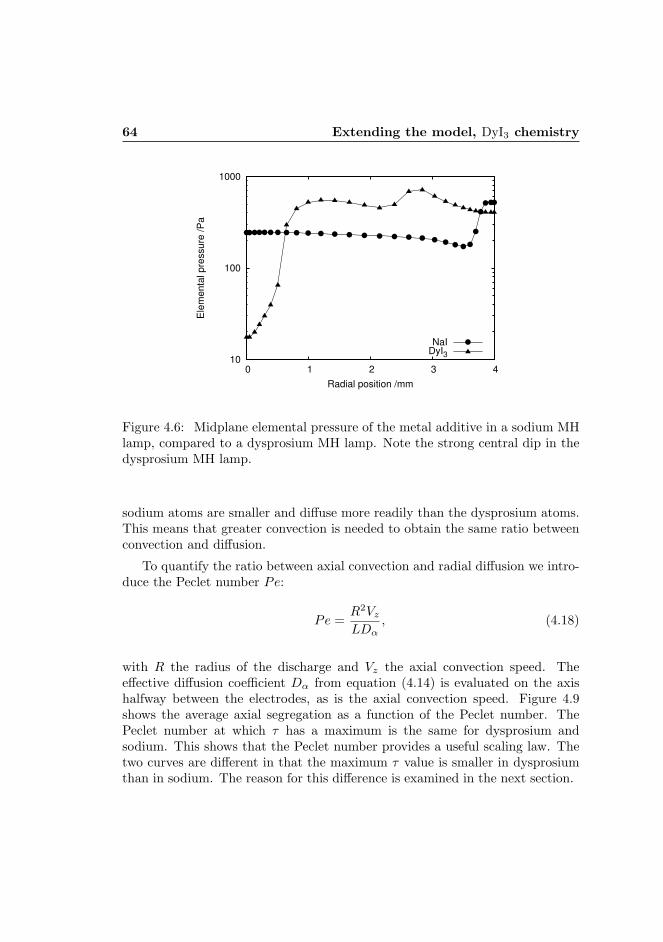
64 Extending the model, DyI3 chemistry
10
100
1000
0 1 2 3 4
Ele
menta
l pre
ssure
/P
a
Radial position /mm
NaIDyI3
Figure 4.6: Midplane elemental pressure of the metal additive in a sodium MHlamp, compared to a dysprosium MH lamp. Note the strong central dip in thedysprosium MH lamp.
sodium atoms are smaller and diffuse more readily than the dysprosium atoms.This means that greater convection is needed to obtain the same ratio betweenconvection and diffusion.
To quantify the ratio between axial convection and radial diffusion we intro-duce the Peclet number Pe:
Pe =R2Vz
LDα, (4.18)
with R the radius of the discharge and Vz the axial convection speed. Theeffective diffusion coefficient Dα from equation (4.14) is evaluated on the axishalfway between the electrodes, as is the axial convection speed. Figure 4.9shows the average axial segregation as a function of the Peclet number. ThePeclet number at which τ has a maximum is the same for dysprosium andsodium. This shows that the Peclet number provides a useful scaling law. Thetwo curves are different in that the maximum τ value is smaller in dysprosiumthan in sodium. The reason for this difference is examined in the next section.

4.5 Results 65
0
1
2
3
4
5
6
0 5 10 15 20 25 30
Segre
gation d
epth
Pressure / bar
NaIDyI3
Figure 4.7: Dimensionless segregation depth as a function of lamp pressure fora dysprosium MH lamp compared with sodium MH lamp results from chapter3.
4.5.2 Convection
The convection patterns in the lamps studied are also altered by the additives.This is demonstrated in figure 4.10 which shows the axial convection throughthe midplane 4.10. The mercury lamp shows a slightly larger convection speedthan the sodium lamp due to the hotter centre. The reason for this hotter centreis the less effective radiative cooling of the mercury plasma due to the absence ofstrong radiators. The dysprosium causes the arc to contract, leading to an evenhotter centre, and thus even stronger convection. Figure 4.11 shows the axialconvection compared to the location of the molecules, atoms, and ions in thedysprosium MH lamp. Note that the area with downward convection containsmostly molecules. The transition to atoms occurs in a position where the netflow is towards the top of the lamp. The point of transition is also the pointwhere the gradients of the partial pressures of atoms and molecules are largest.In a sodium lamp, as shown in figure 4.12, the transition from molecules toatoms is much closer to the walls. This means that the downward flow nearthe walls contains more atoms than in the dysprosium discharge. Molecules arenot present in the upward flow. Thus, axial segregation is more pronounced inthe sodium containing discharges than in the dysprosium containing discharges.

66 Extending the model, DyI3 chemistry
0
5e-05
0.0001
0.00015
0.0002
2 4 6 8 10 12 14 16 18 20 22
Diffu
sio
n c
oeffic
ient / (m
/s2)
Pressure / bar
NaIDyI3
Figure 4.8: Diffusion coefficient on the axis halfway between the two electrodesfor dysprosium and sodium atoms compared.
This difference explains the difference in the segregation depth at the samePeclet number found in figure 4.9.

4.5 Results 67
0
1
2
3
4
5
6
0 0.5 1 1.5 2 2.5 3 3.5 4 4.5 5 5.5
Se
gre
ga
tio
n d
ep
th
Peclet number
NaIDyI3
Figure 4.9: Dimensionless segregation depth as a function of the Peclet numberfor a dysprosium MH lamp compared with sodium MH lamp results in chapter3.

68 Extending the model, DyI3 chemistry
-0.1
-0.05
0
0.05
0.1
0.15
0.2
0.25
0.3
0 1 2 3 4
Axia
l velo
city / (
m/s
)
Radial position /mm
pure HgNaI
DyI3
Figure 4.10: Axial convection through the plane halfway between the twoelectrodes. The difference between the lamps containing dysprosium and thelamp containing sodium is substantial. The lamp containing pure mercury hasa slightly higher convection speed than the sodium lamp due to the hotter centre.

4.5 Results 69
1e+20
1e+21
1e+22
1e+23
0 1 2 3 4-0.1
0
0.1
0.2
0.3
density / m
-3
velo
city / (
m/s
)
radial position /m
DyI3DyI2
Dy
Dy+
vz
Figure 4.11: The transition from molecules to atoms and from atoms to ions in adysprosium MH lamp compared with the axial velocity. The relevant transitionsare indicated with the dotted vertical lines. Note that transition from moleculesto atoms occurs in the upward directed flow.

70 Extending the model, DyI3 chemistry
1e+21
1e+22
1e+23
0 0.001 0.002 0.003 0.004-0.05
0
0.05
0.1
0.15
density / m
-3
velo
city / (
m/s
)
radial position /m
Na+
Na
NaIVz
Figure 4.12: The transition from molecules to atoms and from atoms to ionsin a sodium MH lamp compared with the axial velocity. The transitions areindicated with the dotted vertical lines. Note that the transition from moleculesto atoms is closer to the wall than in the dysprosium MH lamp.

4.5 Results 71
1000
2000
3000
4000
5000
6000
7000
Tem
pera
ture
/K
Radial position /mm
Axia
l positio
n /m
m
NaI DyI3
-4-3-2-1 0 1 2 3 4
0
5
10
15
20
Figure 4.13: The temperature of a dysprosium MH lamp compared with asodium MH lamp. Both lamps have a total mercury filling of 20 mg and aredriven with a power of 135 W.

72 Extending the model, DyI3 chemistry
2000
3000
4000
5000
6000
7000
0 5 10 15 20
Tem
pera
ture
/K
Axial position / mm
pure HgNaI
DyI3
Figure 4.14: Temperature on the axis of a pure mercury lamp, a sodium MHlamp and a dysprosium MH lamp compared. All lamps have a total mercuryfilling of 20 mg and are driven with a power of 135 W.

4.5 Results 73
1000
2000
3000
4000
5000
6000
7000
0 1 2 3 4
Tem
pera
ture
/K
Radial position /mm
pure HgNaI
DyI3
Figure 4.15: Comparison of the temperature midplane between the two elec-trodes for a pure mercury lamp, a sodium MH lamp and a dysprosium MHlamp. All lamps have a total mercury filling of 20 mg and are driven with apower of 135 W.
4.5.3 Temperature
All quantities in the LTE model are connected to the temperature distribution.The convection speed, in particular is driven by the large temperature differencebetween the wall and the hot centre. The dysprosium lamp shows less axialsegregation than the sodium lamp. This has an effect on the axial temperatureprofile shown in 4.14. The temperature of the dysprosium MH lamp varies littlealong the axis while the sodium containing discharge is much hotter at the topthan at the bottom. This is because little to no sodium is present near thetop electrode. Thus, in the sodium containing discharge, the temperature nearthe top electrode approaches that of a pure mercury discharge. Additionally,the presence of dysprosium causes the arc to contract. This is because a lot ofradiation is released just off-centre where most excited atoms are present. Thecentre contains few atoms and the mercury ions push the dysprosium ions outof the centre, leading to the strong central dip shown in figure 4.6. The centraltemperature must be higher than in a pure mercury lamp to still allow sufficientcurrent to pass through the plasma. For comparison, the temperature of a puremercury discharge is also shown in figure 4.14.The midplane radial temperature profiles in figure 4.15 show the contractionmost clearly. The pure mercury lamp has a parabolic temperature profile. Thesodium MH lamp is slightly flattened, and the dysprosium MH lamp showsstrong contraction. The dysprosium MH lamp shows the hottest central tem-perature, followed by the pure mercury lamp and the sodium MH lamp has thelowest central temperature.

74 Extending the model, DyI3 chemistry
4.6 Conclusions
Using plasimo a model of an MH lamp based on a mixture of dysprosium iodideand mercury has been built. The chemical composition has been calculatedusing the Gibbs minimisation approach. From this chemical composition thedominant species have been determined. Comparison with earlier results showsthat the pressure for which the axial demixing is most pronounced is lowerin lamps containing dysprosium than in lamps containing sodium additives.This is because the dysprosium atoms move less easily through the backgroundmercury gas and have lower diffusion coefficients than the sodium atoms. Themaximal axial segregation of the dysprosium lamps is slightly smaller than theof the sodium containing discharges. The reason for this is that the temperaturerequired to fully dissociate the dysprosium tri-iodide molecules is higher thanthe temperature to dissociate the sodium iodide molecules. Additionally, thedysprosium additives cause strong contraction in the arc. Thus, the moleculesdissociate further away from the walls with molecules not only dragged downby convective flows near the walls, but also pushed upwards.
The temperature profiles of a lamp containing dysprosium additives differmuch from the temperature profiles of a lamp containing sodium. This is be-cause of radiative cooling of atomic dysprosium, just off-centre. The centralpart of the discharge contains little to no dysprosium and is thus less effectivelycooled. To allow enough current through the lamp the central temperature mustbe greater than in a pure mercury lamp. Another difference occurs from thedepletion of additives near the top of the sodium containing lamp. The part ofthe discharge devoid of additives approaches the temperature of a pure mercurydischarge.
The Peclet number, defined as the ratio of axial convection to radial diffusionmay be used to predict the conditions under which axial segregation is greatest.Radial segregation plays a central role in the development of axial segregation.The position at which the molecules dissociate to form atoms has an importantinfluence on the degree of segregation. When molecules dissociate in the part ofthe lamp where the convection current moves downward the axial segregationis more pronounced than when they dissociate further from the walls, into theradial position where the convective flows are towards the top of the lamp.

Chapter 5
Radiation
Abstract. The radiation emitted by a lamp containing mercury and dys-prosium additives is studied. Dysprosium has a spectral ”grass field” withhundreds of lines, which are mostly optically open under the conditions stud-ied. Mercury emits radiation on a small number of lines which may be op-tically open, closed or in between, depending on the exact conditions. Weintroduce effective transitions for the radiation emitted by the dysprosiumadditive. These effective transitions are used in combination with ray tracingto model the radiation transport of resonant and partially absorbed mercurylines. The errors introduced by using effective transitions instead of simulat-ing all known transitions is studied through a number of simple case studies.The effective dysprosium transitions are then used in a self consistent modelof a metal halide lamp. The choice of data set has a significant impact on theresult. Using the data from Gorschkov et al leads to stronger arc contractionthan using the more recent data from Wickliffe et al. The distribution ofadditives is also effected by the choice of input data.

76 Radiation
5.1 Introduction
In chapter 2 we presented a study that describes axial segregation in MetalHalide lamps. One of the findings was that increasing the pressure increasesconvective flows in the lamp. When the convective flows are strong enoughthe elements become homogeneously mixed, both radially and axially. At lowpressures axial demixing is avoided, but radial demixing is still present. Themodel can be used to predict the range of pressures that should be avoided whendesigning a lamp. A disadvantage of the model presented in chapter 2 was thatthe electrodes are approximated by two flat planes.
In chapter 3 we improved the model by taking the shape of the electrodeinto account. This model with penetrating electrodes was run for a series ofconditions and it was found that the electrodes influence convection patternsin the lamp. By changing the convection patterns the competition betweenconvection and diffusion is also changed, and thus also the degree of segregationin the lamp. Not only the competition between convection and diffusion isdeterminative for the segregation in the lamp. The temperature profile also hassome influence. However, this temperature profile is not only determined bythe fluid transport processes, the radiation also has a large effect on this profile.Especially the correct treatment of radiation transport deserves attention.
For a part of the spectrum the plasma will be optically thick so that thegenerated emission is locally re-absorbed whereas for another part radiationcan easily escape. For a correct description of both the optical thin and thickradiation we used the method of ray spacing [41].
The models in chapters 2 and 3 were based on MH lamps consisting ona mixture of Hg and NaI. The number of atomic lines in this plasma type islimited. This implies that the ray-trace method can be restricted to a limitednumber of frequency points.
To compare with experiments the authors have changed the model so that itwill work with dysprosium iodide. The primary reason for this is that we wishto compare results with the measurements in [21], which uses, amongst others,the technique of X-Ray Fluorescence (XRF) to measure the elemental densities.This technique works with heavy elements such as mercury and dysprosium butnot with sodium. A plasma containing dysprosium additives, however, is moredifficult to model than one containing sodium for two reasons:
• A plasma with dysprosium additives has more intermediate molecularspecies, and these molecules are more complex. To overcome this diffi-culty we used lookup tables in conjunction with external chemical equi-

5.2 Model description 77
librium calculations to calculate the chemical composition of the plasmaas described in chapter 4.
• Dysprosium atoms and ions have a large number of radiative transitions.The data set of Wickliffe, Lawler and Nave [44] lists over 900 lines andthese represent only the most prominent transitions.
In this chapter we will focus on this last issue. Fortunately, the myriad ofspectral lines from dysprosium atoms and ions are, for the relevant conditions,optically open. As will be shown, effective transitions can be used to model theradiative energy emitted by the plasma. This method allows a great reductionin the complexity of the calculation. Before further discussing the use of effec-tive transitions we will first give a general overview of treatment of radiationtransport in the model. Then we will investigate the validity of the use of ef-fective transitions via simple test models. We will conclude with results from afull calculation employing these effective transitions for two different sources ofdata.
5.2 Model description
In this section we give a short overview of the treatment of radiation transport inthe model and its interaction with the calculation of fluid properties. The modelsolves conservation equations to obtain the temperature, velocity and additivedistribution in the lamp. More details are found in chapter 2. A schematic viewof the geometry and grid used is given in figure 5.1.
5.2.1 Energy balance
All modules come together in the energy balance to calculate the plasma temper-ature. The temperature, in turn, strongly influences the transport coefficients,composition, flow and radiation. The temperature is given by
∇ · (Cp~u∇T ) −∇ · (λc∇T ) = P − Qrad, (5.1)
where Cp is the heat capacity at constant pressure, λc the thermal conductivity,Qrad the net radiated power 1 and P the Ohmic dissipation. To obtain boundaryconditions for equation 5.1 a cold spot temperature of 1100 K is assumed, with
1Note that in this work Qrad is defined such that it is positive if more radiation is emittedthan absorbed, contrary to the convention employed in [41].

78 Radiation
Electrodes
4 mm
20
mm
18
mm
Figure 5.1: Schematic view of the geometry of the problem (not to scale) andthe finite volume grid used. The actual grid used is less coarse than suggestedin this figure. The computation grid has 66 cells in the axial and 28 cells in theradial direction.
the cold spot located in the bottom corner of the lamp. The electrodes areassumed to have a surface temperature of 2900 K and the rest of the wall atemperature of 1200 K.
5.3 Radiation transport
The term represented by Qrad in (5.1) is the primary focus of this chapter. Itis the net result of local emission and absorption at every point in the plasma.To calculate the net radiated power we need to consider the energy gainedby absorption of light emitted elsewhere and the energy lost by light emittedlocally at each point in the plasma. Since emission and absorption are stronglyfrequency dependent we also need to do this for a large number of differentfrequencies and integrate over frequency space.

5.3 Radiation transport 79
The net radiated power is related to the radiation intensity Iν by [41]:
Qrad =
∫
ν
(
4πjν(ν, ~r) −
∫
4π
κ(ν, ~r)Iν(ν, ~r)dΩ
)
dν, (5.2)
with ν the frequency, jν(ν, ~r) the local emission coefficient and κ(ν, ~r) the localcoefficient for absorption along rays passing through the discharge. Note thatthe subscript ν is used to denote a quantity per unit of frequency.
The radiation intensity Iν is determined by [41]
dIν
ds= jν − κIν . (5.3)
5.3.1 Ray tracing on a structured mesh
To solve equation (5.3) we use the method of ray tracing, as outlined in [41].This method was originally implemented for discharges with two degrees ofsymmetry. The code has since then been modified to describe two dimensionalplasmas with only rotational symmetry. We will briefly outline our ray tracingmethod following [41] and discussing the modifications implemented.
Radiation transport in plasmas is essentially non-local: every point in theplasma may absorb photons from any other point in the plasma. This standsin contrast with other fluid properties of which the transport can be handledlocally. That is, these properties, such as the density or the temperature, de-pend only on the local value and the local gradients. The finite control volumemethod works well for such local properties: the temperature in a control vol-ume, for example, is assumed to be influenced only by the control volumes in thedirect neighbourhood. The plasma properties are defined on the nodal points.Transport, or fluxes, of conserved properties, take place through the surfaces ofthe cells.
The Ray Tracing Control Volume rtcv method describes the interplay be-tween the local properties of the fluid and the non-local radiation by combiningray tracing for the radiation transport with finite control volumes on structuredmeshes for the fluid properties.
Ray tracing describes the intensity of the radiation by calculating this inten-sity along a series of probe lines through the plasma. This is done by integrating(5.3) along the probe lines. By clever use of the presence of symmetry the num-ber of probe lines may be limited. The local emission and absorption along eachsegment of the ray is determined from the fluid property in the control volumesthrough which the ray passes. The rtcv method consists of a number of steps.

80 Radiation
1. The choice of probe lines which follows from the symmetry of the prob-lem. This step does not need to be repeated during the iterative solutionprocedure as long as the grid remains the same.
2. The integration of (5.3) along each probe line. The coefficients jν and κalong each segment of the probe line are given by the fluid properties inthe control volume through which the probe line passes.
3. The calculation of the radiative fluxes through the boundaries of eachcontrol volume given the intensity and the solid angle carried by the rays.The net radiated power Qrad follows from the difference in the radiativefluxes through the boundaries.
4. The calculation of fluid properties on the CV mesh given Qrad. From thisstep new values of jν and κ follow.
5. Test for convergence, if convergence is not reached go back to step 2.
5.3.2 The choice of probe lines
The MH lamps under study are assumed to be rotationally symmetric. Thisrotational symmetry may be exploited in the choice of probe lines. In particular,the set of probe lines originating from a point may be re-arranged into a set ofparallel lines, or chords, as shown in figure 5.2. The one dimensional code useda single parallel set of chords as the coefficients jν and κ are independent of theaxial coordinate in the one dimensional case. To account for the dependence onthe axial coordinate the code has been modified by using sets of parallel raysat multiple angles to the axis (21 different angles are used in practice) for eachaxial position in the grid. We chose an uneven number of angles with the axisso that we do not have rays parallel to the axis. A schematic representation isgiven in figure 5.4.
5.3.3 Integration along the probe lines
After choosing a suitable set of rays through the plasma the intensity is calcu-lated by integrating (5.3) along these rays: [50, page 10]
Iν(~r, ~Ω) =
∫ ∞
0
jν(~r − s~Ω) exp
(
−
∫ s
0
κ(~r − s′Ω)ds′)
s. (5.4)
The cylindrically symmetric control volume grid discretizes the plasma intoconcentric cylinders. The coefficients jν and κ depend on plasma parameters
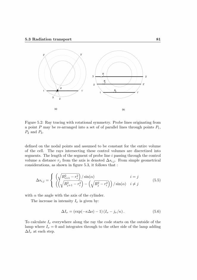
5.3 Radiation transport 81
1
23
3’
1’
2’
P
P
P
1
2
31
2
P31’
2’
3’
(a) (b)
Figure 5.2: Ray tracing with rotational symmetry. Probe lines originating froma point P may be re-arranged into a set of of parallel lines through points P1,P2 and P3.
defined on the nodal points and assumed to be constant for the entire volumeof the cell. The rays intersecting these control volumes are discretized intosegments. The length of the segment of probe line i passing through the controlvolume a distance rj from the axis is denoted ∆si,j . From simple geometricalconsiderations, as shown in figure 5.3, it follows that :
∆si,j =
(√
R2i+1 − r2
i
)
/ sin(α) i = j((√
R2j+1 − r2
i
)
−(√
R2j − r2
i
))
/ sin(α) i 6= j(5.5)
with α the angle with the axis of the cylinder.
The increase in intensity Iν is given by:
∆Iν = (exp(−κ∆s) − 1) (Iν − jν/κ) . (5.6)
To calculate Iν everywhere along the ray the code starts on the outside of thelamp where Iν = 0 and integrates through to the other side of the lamp adding∆Iν at each step.

82 Radiation
α
∆ s i,i
ri
iR
∆ si,j
Ri−1
(b)(a)
Figure 5.3: The length of the line segment through a control volume cell. Figure(a) shows a three dimensional view of a single ray at an angle α to the axis.Figure (b) shows two rays, one passing through a control volume only once, andone crossing the same control volume twice.
5.3.4 Radiative fluxes
After integrating along each probe line the intensity Iν along the probe lines isknown. From this intensity the radiative fluxes through the walls of the controlvolume boundaries can be calculated. The radiative flux through the boundariesis given by the intensity and the surface area of the cell.
In general terms, the radiative flux through a surface with area A and normal~n by a beam with solid angle d~Ω is given by [41]:
Φεν = A~n · d~ΩIν . (5.7)
In the case of our cylindrical control volume grid the discretized form of theabove equation becomes:
Φεν = 2Iν
dy
rdrsin2 αdα, (5.8)
with dy the distance between chords in the plane, as shown in figure 5.4.The term Qrad follows from the difference in the flux of radiation on the cell
boundary points:
Qrad,ν =1
V(Φε
ν(s + ds) − Φεν(s)) , (5.9)

5.3 Radiation transport 83
with Φεν the radiative flux and V the volume of the cell.
The current design of the RTCV code is a direct evolution from the originalspherically symmetric ray tracing code by Van der Heijden [41]. In this, originaldesign, the decision was made to calculate the radiative fluxes through the wallsof the control volumes instead of directly calculating Qrad on the nodal pointsfrom the intensity. In the case of point symmetry the approach of calculatingthe fluxes first and then the net radiated power is more accurate for reasonsoutlined in [41]. In principle, it is also possible to calculate Qrad directly on thenodal points of the grid, as also outlined in [41]. This latter approach would,in some ways, be more flexible than the current method. Future plans includerefactoring the current code to be more general in terms of the geometry of theproblem.
α
top−viewside−on view
b ca
dr
ds
Figure 5.4: Schematic representation of ray tracing on the two dimensionalcylindrically symmetric grid. Viewed from the top (c), the projections of therays follow chords through the cylinder interspaced with distance dy. Thesechords are repeated at each axial grid position for a number of different angleswith respect to the axis, as shown in the schematic of the side-view (a). Theside view shows just two sets of rays for the central chord to minimise clutter.Also shown is a single ray passing through the concentric cylinders which makeup the finite volume grid (b).

84 Radiation
5.4 Ohmic heating
The power to the plasma is supplied by Ohmic heating P = σE2. We solve thePoisson equation in the form:
∇ · (σ∇Φ) = 0, (5.10)
with Φ the potential (∇Φ = − ~E). The boundary conditions are formed byconstant Dirichlet conditions of 100 V on one electrode and 0 V on the otherelectrode. The upper value of 100 V is adjusted in an iterative manner to arriveat an integrated power dissipation of 130 W. The current through the walls iszero. Thus on these boundaries a homogeneous Neumann boundary conditionis used.
~J · ~n = σ∇Φ · ~n = 0. (5.11)
In an area a distance of 0.5 mm around the electrodes the conductivity isadjusted to compensate for non-LTE effects. This is necessary since the electrondensity near the electrodes will deviate significantly from the values expectedfrom chemical equilibrium. High temperature electrons travel to the electrodes,leading to electron temperatures and densities approaching those of the hot spotjust in front of the electrode. Thus, the actual electrical conductivity will beclose to the electron conductivity in the hot plasma near the cathodes, and notequal to the conductivity calculated by the assumption of LTE. Not correctingfor the increased conductivity at the electrodes would effectively couple all theelectrical energy in the first layer of cells near the electrodes, overestimatingthe temperature in these cells, while underestimating temperature elsewhere. Acorrection is made by imposing a minimal conductivity in a small area aroundthe electrode of 40 Ohm/m. This value corresponds to the electrical conductivityat 4000 K.
5.5 Effective transitions
Adding dysprosium to a plasma results in a spectral ”grass-field”. We willinvestigate to what extent this myriad of lines can be approximated by a singleformula describing the net radiated power how this will effect the temperaturedistribution and how this will lead to different temperature profiles and thus todifferent convection patterns and additive distributions. From previous studieswe know that for dysprosium containing MH lamps a large part of the radiationis generated by dysprosium atoms (Dy I) and dysprosium ions (Dy II) lines and

5.5 Effective transitions 85
that most of this radiation can freely escape from the plasma. Throughout thispaper we will assume that within an atomic (or ionic) system the levels arepopulated according to Boltzmann. We will at first consider Dy I and Dy II asseparate systems, and then study the result of the two combined. In particular,we will study the radiated power per particle (RPP) in each system. First wecalculate the RPP using transition probability data from literature. This is doneusing two different literature sources: [44] and [51] and for the systems DyI andDy II separately. We will show that the effect of literature source-selection onthe plasma shape is substantial. To enable a more systematic study of the effectof the RPP and the impact of the different sets of transition probability sourcesanalytical fit functions of these RPP will be presented.
To this end we examine the error made by approximating Qrad by a limitednumber of optically thin transitions. This is done through three case studies:
1. a sphere at a uniform temperature containing dysprosium vapour,
2. a sphere containing both mercury and dysprosium at a uniform tempera-ture and
3. a cylinder with a radially dependent temperature profile and an axiallyvarying dysprosium concentration.
In the case of optically thin transitions, radiation presents a simple localenergy loss term to the energy balance of the plasma. This is the case for afrequency ν if the optical depth at that frequency τ(ν) =
∫
κ(ν)ds is muchsmaller than unity. In this case, we may ignore absorption so (5.3) becomes
dIν
ds= jν = (hν/4π)nuAulφul,ν(ν), (5.12)
with nu the density of the upper state, Aul the transition probability and φul,ν
a normalised line broadening profile∫∞
0φul,νdν = 1.
In the following the ion and atoms systems are treated separately. If theemitting system has an internal Boltzmann energy distribution with tempera-ture T , the density of the upper level is given by the Boltzmann balance forexcitation [31]
nu =nSgu
QSexp
(
−Eu
kT
)
, (5.13)
with nS the density and QS the partition function of the atomic or ionic system.The partition function is given by
QS =∑
p
gp exp
(
−Ep
kT
)
(5.14)

86 Radiation
with gp the degeneracy of level p. The summation runs over all levels in thesystem. In theory, the number of levels is infinite. To calculate the partitionfunction a cutoff is required. We simply limit the sum to the highest upper levelfrom which a radiative transition is in the dataset.
5.5.1 Radiated power per particle
We will now examine the RPP in each system. The energy radiated is given byintegrating over the frequency spectrum for all transitions.
Qrad =
∫
∑
u
∑
l
(hνulnuAulφul,ν(ν)) dν. (5.15)
If no radiation is absorbed this is equivalent to the summation over all transitionswithout line broadening. Making use of (5.13) we obtain
Qrad
nS=∑
u
gu
QSexp
(
−Eu
kT
)
∑
l
Aulhνul. (5.16)
This quantity is the RPP, which we will seek to replace with a simple approxi-mation. We replace (5.16) with an effective transition, as given by
Qrad(T )
nS= Aeff∆Eeff exp
(
−∆Eeff
kT
)
. (5.17)
The parameters ∆Eeff and Aeff are free fit parameters. We calculate the RPPfor fixed system densities and temperatures between 1000 K and 7000 K usingequation (5.16). The parameters ∆Eeff and Aeff are then determined by aleast squares fit through the results. Results of using the double sum in (5.16)on data from [44] are shown in figure 5.5. The best fit of the single expression(5.17) for ∆Eeff and Aeff is also shown in the same figure. The correspondingvalues thus obtained are Aeff = 1.21× 10⁸ Hz for the atoms and 1.43× 10⁸ Hzfor the ions. The resulting effective energies are 2.279 eV for the atoms and2.292 eV for the ions.
In the following subsections the case studies mentioned earlier will be stud-ied. In the case studies the radiated power is determined by use of the effectivetransitions just derived and compared with results from the full set of data. Allthe case studies assume that the plasma is in LTE. Thus, the radiation emit-ted is fully determined by the elemental composition and temperature in the

5.5 Effective transitions 87
0
2e-13
4e-13
6e-13
8e-13
1e-12
1.2e-12
1000 2000 3000 4000 5000 6000 7000
Ra
dia
ted
po
we
r p
er
pa
rtic
le in
th
e s
yste
m /
W
Temperature / K
Dy+ with data from Wickliffe et alEffective transition Dy+
Dy with data from Wickliffe et alEffective transition Dy
Figure 5.5: Radiated power per particle for both the dysprosium atom (Dy I)and dysprosium ion (Dy II) systems. To calculate the energy loss the densitiesof the ground state where fixed and a Boltzmann distribution of the excitedstates was assumed. The free parameters from equation (5.17) are determinedby fitting this equation through the results. The result of this fit is also shownin figure 5.5. The resulting fit yields an effective transition probability of 1.21×10⁸ Hz for the atoms and 1.43 × 10⁸ Hz for the ions. The resulting effectiveenergies are 2.279 eV for the atoms and 2.292 eV for the ions.
plasma. The distribution of dysprosium over the two systems is determined bythe Saha balance,
nenDy+
2nDy=
QDy+
QDy
(
2πmekT
h2
)3
2
exp
(
−Ei
kT
)
, (5.18)

88 Radiation
5.5.2 Sphere filled with dysprosium
The first case study is formed by regarding the radiation emitted by a sphereof dysprosium vapour at a uniform temperature, where the plasma may beregarded as optically thin. The total dysprosium pressure is fixed at 1000 Pa.The distribution over the ion and atom systems is determined by the Sahabalance, with the partition function calculated from the atomic levels from [44].The electron density is determined by assuming quasi-neutrality ne = nDyII .Only dysprosium atoms, singly ionised atoms, and electrons are considered. Thedensities thus obtained are shown in figure 5.6.
Figure 5.7 shows the radiation emitted in the first case study. This figureshows the RPP calculate two ways, by use of (5.16) and with (5.17). As ex-pected, the agreement between the two approaches is excellent. Effectively, thiscase study is the inverse of the procedure which determines the coefficients forthe effective transitions.
5.5.3 Sphere with dysprosium and mercury
Using these results in a plasma containing other radiative species is, however,slightly more problematic. Other species, such as mercury, may absorb radia-tion emitted by dysprosium. To examine the possible error, results are comparedagain in a second case study for a sphere containing mercury as well as dyspro-sium. We again look at a sphere of uniform temperature with a volume of 1cm3
containing dysprosium and mercury. The elemental abundance of mercury is1,000 times that of a dysprosium . The total pressure is chosen at 10 bar. Onedimensional ray tracing is used to calculate the energy loss term for tempera-tures from 1000 K to 7000 K. Full ray tracing is done on all lines, but for theoptically open lines only three frequency points are chosen. The ion densitiesare given by the Saha balance. The resulting net radiated power is shown infigure 5.8. The match between the effective transition approach and the fulldata set is again very good at higher temperatures.
5.5.4 Cylinder with dysprosium and mercury
In metal halide lamps the temperature is far from constant. To examine a situ-ation closer to that of a metal halide lamp a third case study will be performed.A parabolic temperature profile
T (r) = Twall + TA
(
1 − (r/R)2)
. (5.19)

5.5 Effective transitions 89
10000
1e+06
1e+08
1e+10
1e+12
1e+14
1e+16
1e+18
1e+20
1e+22
1e+24
1000 2000 3000 4000 5000 6000 7000
De
nsity /
m-3
Temperature /K
Density according to the Saha balance
DyDy+
Figure 5.6: Densities from the Saha balance as a function of temperature, usingthe data from [44] to calculate the partition functions. The total dysprosiumpressure is 1000 Pa.
is imposed on a cylinder with a radius R = 5 mm and a length of 10 mm. Thecoefficients are Twall = 1200 K, TA = 4800 K, The cylinder has an exponentiallydecaying dysprosium pressure in the vertical direction given by
p = p0 exp(−z/Λ), (5.20)
with p0 = 150 Pa and Λ = 9.0 cm.The net radiated power is then calculated using two effective transitions,
and the complete set of data from [44]. In all cases full two dimensional ray-tracing is used, with three frequency points for the open lines and one hundredfrequency points for each mercury line. On a standard desktop computer thecalculation with the full data set takes close to one hour. As part of an iterativemethod this is unacceptable as full calculations would take years to complete.
The results with the full data set and the effective transitions are shown

90 Radiation
0
1e-13
2e-13
3e-13
4e-13
5e-13
6e-13
7e-13
1000 2000 3000 4000 5000 6000 7000
Ra
dia
ted
po
we
r p
er
pa
rtic
le /
W
Temperature /K
Effective transitionscomplete set
Figure 5.7: Radiated power per particle as a function of temperature for twosystems, Dy I and Dy II. The distribution of dysprosium over the two systems isdetermined by the Saha balance using ne = nDyII . The radiation emitted wasthen calculated using the full set of data from [44] and by effective transitionsfor the atoms and ions. The energy radiated away has been divided by the totalnumber of particles in the system.
in figure 5.9. As may be expected, agreement, though still reasonable, is notas good as in the previous more artificial examples. The mercury vapour mayabsorb radiation emitted by the dysprosium atoms or ions, and this has notbeen taken into account. The differences are small enough, however, to allow theuse of the effective transitions to speed up calculations and generate a properstarting point for more accurate calculations if so desired. Alternatively, anumber of transitions with frequencies that can be absorbed by the mercuryvapour could be added.

5.5 Effective transitions 91
0
2e+10
4e+10
6e+10
8e+10
1e+11
1.2e+11
1.4e+11
1.6e+11
1.8e+11
2e+11
1000 2000 3000 4000 5000 6000 7000 0.001
0.01
0.1
1
10
Ra
dia
ted
po
we
r p
er
un
it o
f vo
lum
e /
(W
/m-3
)
rela
tive
err
or
Temperature / K
effective transitionscomplete set
error
Figure 5.8: Net radiated power by a sphere containing 10 bar mercury and 10mbar dysprosium in LTE. The solid line shows the result with the radiationemitted by dysprosium calculated through (5.17). The dashed line shows theresult using 1 dimensional ray tracing with the data from [44]. As these twolines difficult to distinguish the relative error is also plotted with a dotted line.The relative error is very small at the higher temperatures.
5.5.5 Sensitivity analysis
The last test case was repeated with the values for the effective transition fre-quencies lowered and raised by fifty percent. As can be seen in the graph, theresult is not particularly sensitive to the effective transition probabilities. Rais-ing the transition probabilities for the ion system leads to more emission fromthe centre of the plasma.
Changing the effective energies has more effect. Figure 5.11 shows the effectof changing the effective transition energies by five percent. Fortunately, thetransition energies for the complete system can be measured to an excellent

92 Radiation
-1e+08
0
1e+08
2e+08
3e+08
4e+08
5e+08
6e+08
7e+08
0.0005 0.001 0.0015 0.002 0.0025 0.003 0.0035 0.004
Ra
dia
ted
en
erg
y /
(W
/m-3
)
Radial position /m
Radiation loss mid-plane
effective transitionscomplete set
Figure 5.9: Radiative power Qrad mid-plane as a function of the radial positionfor a cylinder filled with mercury and dysprosium. A radial parabolic tempera-ture profile has been imposed as well as an exponentially decaying dysprosiumabundance in the axial direction. Near the axis the match between the effectivetransitions and the complete calculations is good, but towards the walls wherethe temperature is lower a mismatch due to absorption becomes apparent.
degree of accuracy.
5.5.6 Choice of data set
As mentioned earlier, other data sets are also available. One of the most widelyused, due to its easy availability online is the set from Gorschkov [51] availableonline via the Kurucz database. This set is much older than the set fromWickliffe et al [44]. We repeated the fitting procedure with the set from [51]. Ascan be seen in figure 5.12 the choice of data set has a large effect on the estimateof the radiation emitted. The set of lines in [51] is also larger than the set in

5.5 Effective transitions 93
-2e+08
0
2e+08
4e+08
6e+08
8e+08
1e+09
1.2e+09
1 2 3 4
Qra
d /
W m
-3
radial position / mm
effective transitionsDyI increased 50%DyII increased 50%
Figure 5.10: Radiative power Qrad mid-plane for a cylinder filled with mercuryand dysprosium. Three cases are shown: The straight line shows the result witheffective transition probabilities determined earlier, the dashed line shows theresult with the effective transition probability for the dysprosium atom systemincreased fifty percent, and the dotted line shows the result with the effectivetransition probability for the dysprosium ion system increased by fifty percent.
[44]. To test if the radiation in the latter is underestimated by not includingmany lines with smaller transition probabilities we selected the lines from [51]with a transition probability larger than 1 × 10⁷s−1. As can be seen in figure5.12 the influence of neglecting these lines is marginal. The difference betweenthe two can only be attributed to differences in the transition probability of themost prominent lines.

94 Radiation
-2e+08
0
2e+08
4e+08
6e+08
8e+08
1e+09
1 2 3 4
Qra
d /
W m
-3
radial position / mm
effective transitionsEnergy transition DyI increased 5%
Energy transition DyII increased 50%
Figure 5.11: Radiative power Qrad mid-plane for a cylinder filled with mercuryand dysprosium. Three cases are shown: The straight line shows the resultwith effective transition probabilities determined earlier, the dashed line showsthe result with the effective transition energy for the dysprosium atom systemincreased five percent, and the dotted line shows the result with the effectivetransition energy for the dysprosium ion system increased by five percent.
5.6 Results with a self consistent model
Now that we can estimate the RPP of DyI and DyII with a simple analyticalexpression we will use this expression in a complete self consistent model of theplasma. This allows us to examine the influence of the emitted radiation on thetemperature profile, the convective flow and finally on the additive distribution.
The model was run with a total mercury filling of 10 mg, and a power inputof 135 W using the effective transitions of [44] and [51].

5.6 Results with a self consistent model 95
0
2e-13
4e-13
6e-13
8e-13
1e-12
1.2e-12
1.4e-12
1.6e-12
1.8e-12
1000 2000 3000 4000 5000 6000 7000
Ra
dia
ted
po
we
r p
er
pa
rtic
le /
W
Temperature /K
Gorschkov et al, major linesGorschkov et al
Wickliffe et al
Figure 5.12: The influence of the choice of data set on the RPP. As the figureshows, the influence of the choice of data set is large. Selecting only transitionswith a transition probability greater than 1×10⁷ s−1. does not greatly influencethe result.
5.6.1 Temperature profile
Radial temperature profiles for two different axial positions can be seen in figure5.13. The choice of data set has a significant impact on the contraction ofthe discharge. The contraction is caused by radiative cooling of the flanks,where the largest concentration of excited atoms is found. The ions radiateless energy than the atoms. Additionally, mercury ions in the centre push thedysprosium ions aside, leaving the central region with very low concentrationsof dysprosium. The mercury emits less radiation than the dysprosium leadingto higher temperatures in the centre. The model fixes, as a real lamp ballastwould, the electrical power input into the plasma. A strong arc contraction,therefore requires a higher central temperature to still allow the same current

96 Radiation
to flow through the lamp. The difference in the degree of contraction is mostpronounced near the bottom of the lamp where the concentration of dysprosiumis greater. This is because there is very little dysprosium in the top of the lamp.The reason that the difference is not even greater lies in the strong temperaturedependence of the radiated emission. A larger transition probability results inmore emission, leading to stronger cooling of the centre of the discharge. Thisstronger cooling results in a lower temperature to reach a steady state. Becausethe emission depends exponentially on the temperature, the temperature needsto be only slightly lower to reach a new balance.
1000
2000
3000
4000
5000
6000
7000
8000
0 0.001 0.002 0.003 0.004
Te
mp
era
ture
/ K
radial position /m
Wickliffe et al, 5 mmWickliffe et al, 10 mm
Gorschkov et al, 5 mmGorschkov et al, 10 mm
Figure 5.13: Radial temperature profiles for two axial positions in the lamp:5 mm from the bottom electrode and midplane. Note the strong contraction.
5.6.2 Additive distribution
The radiation emitted by the lamp primarily effects the temperature distribu-tion. The temperature distribution, in turn, drives the convection in the lamp.

5.7 Conclusion 97
This convection affects the distribution of additives. As is shown in figure 5.14,the effect of the choice of data set on the additive distribution is significant.The use of the data by Gorschkov et al leads to less axial segregation. The ra-dial segregation is also effected, where the model result based on the Gorschkovdata shows a local maximum, a local minimum is predicted with the data byWickliffe et al.
5.7 Conclusion
By using effective transitions for the radiation emitted by dysprosium the modelof an MH lamp containing a mixture of sodium and mercury has been modifiedto simulate a lamp containing dysprosium additives. The effective transitionsgive an estimation of the radiated power per particle. The accuracy of thisestimation is primarily determined by the accuracy of the input data. Errorsintroduced by this approach are much smaller than the accuracy of the inputdata. The choice of data set from different literature sources has a large effecton the emission at a fixed temperature. The effect on the predicted temperatureis smaller but still significant. Using the more recent data from [44] leads tolower predicted contraction than the older data from [51]. There is an importantsecondary effect on the distribution of additives; the smaller contraction leadsto larger axial segregation with the data from [44] than with the data from [51].

98 Radiation
1
10
100
1000
0 0.005 0.01 0.015 0.02
Ele
menta
l pre
ssure
/ P
a
Axial position / m
Elemental pressure along the axis
Wickliffe et alGorschkov et al
(a)
10
100
1000
0 0.001 0.002 0.003 0.004
Ele
menta
l pre
ssure
/ P
a
radial position /m
Elemental pressure midplane
Wickliffe et alGorschkov et al
(b)
Figure 5.14: Elementary dysprosium pressure along the axis (a) and midplane(b) for the two data sets of [44] and [51].

Chapter 6
Comparison with
microgravity experiments
Abstract.
The results from optical emission spectroscopy experiments of metal halidelamps under the microgravity conditions on board the international spacestation are compared with the results of a numerical LTE model constructedwith the platform Plasimo. At microgravity there is no convection whichallows for easier modelling and for a separate study of the diffusion-inducedradial segregation effect, undisturbed by convection. The plasma parametersthat were experimentally determined and compared to the model were the Dyatom and ion density, the Hg ion density and the temperature.
The model and experiments applied to a reference lamp burning on aplasma mixture of DyI3 and Hg were found to be in reasonable agreement witheach other. The cross-section for electron-Hg collisions was studied, it wasfound that the Rockwood values give the correct results. Experimental resultsguided a sensitivity analysis of the model for the Langevin cross-sections. Theratio of the ion densities n(Hg+)/n(Dy+) was found to be extremely sensitivefor the cross section of the elastic interaction σ(Hg, Dy+) between the Dy ionand the Hg atom. The sensitivity analysis suggests that equating σ(Hg, Dy+)to a value that is 10% higher than the Langevin cross section is the best choice.We also found deviations from LTE in the outer regions of the plasmas forrelative radial positions of r/R > 50%.
This chapter is based on a publication submitted on invitation to a JPhys. D. Special issue as ”Metal-halide lamps in microgravity, experimentand model” with co-authors T. Nimalasuriya, W. W. Stoffels and J. J. A. M.van der Mullen.

100 Comparison with microgravity experiments
Figure 6.1: (a) Colour separation in an MH lamp burner. (b) Schematic viewof an MH lamp; diffusion and convection of atoms (A) and molecules (M) areindicated by arrows.
6.1 Introduction
The metal halide (MH) lamp [25, 52, 53] combines the high luminous efficacy andgood colour rendering of the fluorescent lamp with the compact and high-powercharacteristics of the high-pressure Hg lamps. The lamp contains a rare gasfor starting and a Hg buffer gas plus a small amount of metal-halide additivessuch as DyI3, TlI, or NaI. Even though the additive density is much less thanthe mercury density, most light is emitted by the metals in the visible region,which results in a very high power efficiency (up to 40%). However, despite theclear advantages, the growth of the MH lamp has been hampered by a numberof limitations. One of these is the segregation of colours [5] caused by thenon-uniform distribution of the additives over the lamp due to the competitionbetween diffusive and convective processes, see figure 6.1.
To be able to unravel the complex interaction between convection and dif-fusion, experiments under microgravity conditions have been performed at theinternational space station. In absence of gravity, convection is eliminated, sothat the effect of diffusion can be studied exclusively and the problem is greatlysimplified. The MH lamp in microgravity is therefore easier to model. By com-paring the model results to the experiments we can gain insight into the complextransport phenomena in the MH lamp. The experiments verify the model re-sults, whereas the model aids the interpretation of the experimental results.The experiments are part of a poly-diagnostic study [54, 55, 11, 12, 21, 21] of

6.1 Introduction 101
the MH lamp.
In this paper we present the comparison between the experiments performedon MH lamps under microgravity conditions and a numerical model. The ex-periments were performed in the microgravity environment of the internationalspace station (ISS). The lamp was investigated by means of optical emissionspectroscopy, which yields line intensities of the species Hg, Dy and Dy+. Fromthe calibrated Hg line intensity measurements we constructed radial temper-ature profiles. By combining the temperature profile with the calibrated lineintensities for Dy we obtained absolute radial density distributions of the Dyand Dy+ systems. All measurements were done for different powers rangingfrom 70 to 150 W. The results were reported in [12].
Metal halide lamps come in various shapes and sizes. To be able to compareresults of experiments done on MH lamps and to compare the results from mod-els to the experiments a reference lamp has been defined within the frameworkof the European project COST-529 [9]. The lamp was filled with an Hg buffergas and one salt, i.e. DyI3. This lamp has a relatively simple salt system andtherefore the results are easier to compare with the results of the numericalmodel. We base our models on this lamp geometry. The simulation platformused to construct this model is called Plasimo and is described in previous chap-ters. The model simulated the lamp operating with the following conditions:an electrode distance of 18 mm, a power of 130 W and a Hg pressure of 12 bar.
There are a number of input-parameters that are not well known, such as thevapour pressure of the metal-halide salt at the cold-spot position, the transitionprobabilities and the cross-sections for the elastic collisions between charged andneutral particles. The latter is found to be determinative for the segregationphenomenon. The sensitivity of the model results for the elastic collisional cross-section for the Dy ion and Hg atom were tested. Because the cross-sectionsfor the elastic collisions between the Dy ion and the Hg atom are unknown,the Langevin cross-section was used. The sensitivity of this approximation isinvestigated.
This article is organised as follows. Section 6.2 describes the segregationphenomenon. Section 6.3 gives an account of the experiment. Section 6.4 il-lustrates the model. Results from both experiment and model are presentedand discussed in section 6.5. These results include the comparison betweenmodel and experiment of the radial profiles of the arc temperature and abso-lute atomic and ionic densities of Dy. Finally, section 6.6 offers conclusions andrecommendations for future work.

102 Comparison with microgravity experiments
1000 2000 3000 4000 5000 6000 70001019
1020
1021
1022
D
ensi
ty (m
-3)
Temperature (K)
Dy Dy+ DyI3 Hg+
wall mantlecore
Figure 6.2: Theoretical density distribution of Dy atoms, ions and molecules,and Hg ions as a function of temperature at the midplane of a MH lamp. Forclarity, DyI2 and DyI have been omitted.
6.2 Demixing
When the MH lamp is operated, the Hg is entirely vapourised forming thebuffer-gas, whereas the few milligrammes of DyI3 additive do not evaporatecompletely, leaving a liquid salt pool at the coldest spot at the burner wall. Theadditive molecules diffuse from the relatively cool wall (∼ 1200 K) toward thehot region (∼ 6000 K) of the arc where they dissociate. At the centre the atomsare ionised and excited. As Dy atoms diffuse back to the wall they encounter Iatoms in the cooler gas near the walls and recombine back to molecules [52].
Three principal regions can therefore be identified within the radial densitydistribution of elemental Dy [21] (see Figure 6.2). These are 1) the region nearthe wall where DyI3 molecules are predominant, 2) the mantle region betweenthe wall and the arc core where Dy atoms predominate, and 3) the core wherethe Dy is almost completely ionised in the form of Dy+. The molecule DyI is

6.3 The experiment 103
relatively unstable and does not have a dominant presence in any region of thedischarge.
When burned vertically, the discharge emits light that is non-uniform incolour along its axis. This colour segregation, is caused by the interplay betweenconvection and diffusion which ultimately determines the distribution of theplasma species. Let’s first consider the radial distribution. The temperatureprofile, which is high in the centre and rapidly decreases towards the wall, leadsto a hollow profile for the mass density distribution due to the ideal gas law.Another mechanism that influences the radial distribution of elemental Dy isdiffusion. The atoms and molecules have different diffusion velocities. Thesmaller and lighter Dy atoms diffuse faster outward than the larger and heaviermolecules (DyI, DyI2, DyI3) diffuse inward. This difference in diffusion velocityresults, in steady-state, in an even more hollow profile of the elemental densityof Dy; this effect is called radial segregation [5]. Ambipolar diffusion [33], inparticular, causes the ions to diffuse out of the core faster than neutral atomsor molecules diffuse inwards.
The axial distribution of the species is dominated by convection, whichcauses the hot gas to move upwards in the hot centre of the arc and down-wards along the cool wall of the lamp. This movement of the bulk gas drags thehigh concentration of elemental Dy near the wall downwards, whereas the lowerconcentration of Dy in the centre, caused by the radial segregation, is draggedupwards. As a consequence, a high density of elemental Dy accumulates atthe bottom of the arc, a phenomenon which is known as axial segregation [5].The combination of radial and axial segregation is shown in figure 6.1(b). Thelatter obviously only occurs in presence of convection. Since there is no convec-tion under microgravity conditions axial segregation does not occur, but radialsegregation does.
6.3 The experiment
In the ISS experiment, emission spectroscopy was performed on a MH lamp [9],which is as mentioned above a reference lamp. The lamp consists of a quartzburner of 20 mm in length and 8 mm in inner diameter and a transparent quartzouter bulb. The space between the outer and inner bulbs is vacuum. The burneris made of quartz in order to make the arc optically accessible. The distancebetween the electrodes is approximately 18 mm. The lamp is driven by a 150 WPhilips Dynavision DALI ballast with a 83 Hz square wave current profile, andoperated at different input powers ranging from 70 to 150 W in steps of 20 W. In

104 Comparison with microgravity experiments
Figure 6.3: Setup used for the ISS measurements. It is an Echelle type spectrom-eter in Littrow configuration, the imaging lens (III) is used for the collimationof both the undispersed beam of light as well as the reflected dispersed beam oflight.
a commercial lamp, the burner is often made of PCA (poly-crystalline alumina).PCA can withstand much higher temperatures, allowing the temperature of thedischarge, wall and salt pool to be higher than for a discharge contained by aquartz burner. Therefore, more Dy is expected to be in the discharge in a PCAburner than is the case for burners made of quartz.
An Echelle-type spectrometer was used as there is need for a robust andcompact setup with no moving parts for the experiments at microgravity. Thedownside is that only a few lines could be analysed. A schematic of the Echelle-type spectrometer is shown in figure 6.3 [12]. Its main components are an Echellegrating with a high blaze angle (74), an interference filter for the selection ofthe desired wavelength interval and a CCD camera for imaging. This spectrom-eter was used to measure the absolute intensity of three lines of three differentsystems. These are the 579.07 nm line of the atomic Hg system, and the 642.19nm and the 402.44 nm line of the atomic and ionic Dy system respectively;shortly denoted by the Dy and Dy+ system. The Hg line is used for the deter-mination of the radial temperature distribution, and combined with the lines ofDy and Dy+ the densities of the Dy and Dy+ systems can be determined.
The procedure is as follows, first the transition-integrated intensity of theline emitting species is determined as a function of lateral position. After Abel

6.3 The experiment 105
inversion this gives the radiant power of the transition
Upq(r) = np(r)Apqhνpq (6.1)
from which, np(r), the radial distribution of the radiating level can be deter-mined since the transition probability Apq and the photon energy hνpq of thetransition are known. The density of the system to which the radiating levelbelongs can now be determined using the Boltzmann relation
nS(r) =Upq(r)Q(T (r))
gpA(p, q)hνpqexp
(
Ep
kT (r)
)
, (6.2)
where nS is the system density of an emitting atom or ion, gp the statisticalweight of upper level p, A(p, q) is the transition probability of the transition,hνpq the energy of the emitted photon, Ep the excitation energy of the radiatinglevel, k the Boltzmann constant and T is the temperature. Q(T ) is the partitionfunction of the considered atomic or ionic system. Upq is the radiant power andis determined experimentally, while Q(T ), gp and A can be found in literature[44, 51].
In case of the 579 nm transition of Hg this expression can be used to findthe radial distribution of the temperature T (r). This is done by replacing theleft-hand-side of equation 6.2 by p/kT (r) which is justified since the atomicHg system delivers by far the most particles in the lamp so that Dalton’s’ law,p =
∑
nkT , reduces to p = nHg(r)kT (r). This bulk pressure can be assumedconstant over the lamp. Since Upq(r) is known as function of radial positionwe can use equation 6.2 to determine the temperature as a function of radialposition provided the pressure is known. Since this is not known we follow aniterative procedure. First a guessed value of p is inserted which gives, using themeasured Upq(r), a radial T (r) distribution. In the second step we determinenHg(r) = p/kT (r) which, integrated over the whole volume, gives the totalnumber of mercury atoms NHg in the discharge. In the last step this number,multiplied with the mass of a Hg atom, thus NHgmHg, is compared to the fillingmass MHg. The mismatch MHg/NHgmHg is used to correct the pressure. Withthis new pressure-value we can repeat steps 1 till 3 again. This is done untilconvergence is reached.
Calculation of the radial density profiles is as follows. First the emission ofthe line of interest is measured as a function of lateral position. This profile isthen Abel inverted into a radial intensity profile. The next step depends on thespecies of which the emission line is measured.
In case of the 579 nm line of Hg, the intensity is calibrated and then theabsolute radial intensity profile is used to numerically determine the temperature

106 Comparison with microgravity experiments
profile. In case the atomic or ionic lines of Dy are measured, the temperatureprofile is combined with the calibrated radial intensity profile of the additiveinto an absolute radial system density profile using equation 6.2.
6.4 The model
A description of the model has been published in [40] and [56], reprinted inchapters 2 and 3 where it has been applied to a MH lamp based on a mixtureof Hg and NaI. This model was modified to a simulation of a mixture of Hg andDyI3, as discussed in chapters 4 and 5. One aspect of the model not discussedso far is the calculation of transport coefficients. This section will repeat thetransport equation for the elements and discuss the calculation of the transportcoefficients in the model.
6.4.1 Particle transport
Since we assume LTE, the particle densities may be described by the localtemperature, pressure and elemental composition. Elemental pressure is definedas the pressure that contains all molecular, atomic and ionic contributions of aparticular element. The elemental pressure pα for the element α can be writtenas
pα =∑
i
Riαpi, (6.3)
with pi the partial pressure of the species i, and Riα the stoichiometric coefficient[32]. We solve a conservation equation for the elemental pressure
∇ ·
(
Dα
kT∇pα +
pα
kT~cα
)
= 0, (6.4)
with an effective diffusion coefficient Dα [32]
Dα = p−1α
∑
i
RiαDipi (6.5)
and a pseudo convective velocity cα [32].The diffusion coefficient Di is calculated from the binary diffusion coefficients
Dij by
Di =
∑
j 6=i
(pi/p) /Dij
−1
. (6.6)

6.4 The model 107
The binary diffusion coefficient for the diffusion of species i through species j isgiven by [30, page 486] and depends on the differential cross-section.
In-situ measurements of the elemental pressure at the walls under micrograv-ity conditions are not possible, therefore we assume a Dy elemental pressure atthe wall of 517 Pa and an I elemental pressure of 4268 Pa. These vapour pres-sures were determined with x-ray induced fluorescence measurements at 1g [21].These are assumed to give a good estimation of the vapour pressure at the wallsand are used to fix the boundary conditions.
6.4.2 The selection of cross-sections
In the conservation equations which form the model, important roles are playedby various transport coefficients, such as the diffusion coefficients Di, the ther-mal conductivity λc and the electrical conductivity σel. These transport prop-erties are calculated from collision integrals that are based on differential crosssections [42].
Ideally, one would like differential cross-sections for every possible collisionbetween particles in the plasma. In practice such data is difficult to gatheror calculate since for only a few interactions energy-dependent integral cross-sections σij are available. When available these are used in the model. Forcollisions for which such data cannot be found approximations have to be used.The collisions can be classified along the following categories:
1. Charged - charged collisions; in this case the shielded Coulomb cross-sections is a good and generally applicable approach [33, page 55],
2. Neutral - neutral collisions; there where dedicated cross-section values arenot available these interactions are described as hard sphere collisions,
3. Charged - neutral collisions; this category is the most complicated since, inprinciple, a full quantum mechanical (QM) treatment is needed in which,for instance, the effect of the Ramsauer minimum has to be taken into ac-count. For each pair of interacting particles the QM aspects are different.If results of experiments or QM calculation are not available the use of theLangevin cross-section is the only option. The formula for the Langevincross section reads
σij =
√
παpq2
µijǫ0 (|~vi − ~vj |), (6.7)

108 Comparison with microgravity experiments
with αp the dipole polarisability of the neutral species, q the charge of thecharged species, ǫ0 the permittivity of free space and µij the reduced massµij = mimj/(mi + mj) of the system of colliding particles.
When considering the influence of the cross-section on the values of thetransport coefficients Di, λc and σel it is important to note that Hg atoms formthe most dominant species in the discharge; all other species are present in smallconcentrations.
We begin with the electrical conductivity σel that is mainly determined bythe elastic interactions between electrons with Hg atoms. This electron-Hg in-teraction is of the third category but fortunately the corresponding cross-sectionis well known and it is generally expected that the values from Rockwood [57]are correct within a few percent. We studied whether this is indeed the caseby comparing the results using Rockwood values and Langevin cross-sections.As the value of this cross-section determines the lamp resistance and the ohmicdissipation we calculated the voltage drop over the lamp when the ohmic dissi-pation equals 110 W. This was done for two cases, one based on the Rockwoodvalues and the other on the Langevin cross-section. Using the Rockwood valuesthe model predicts a voltage drop of 99 V, which is consistent with the mea-sured value. The calculations done with the Langevin cross-section, however,produces a voltage drop of 71 V, which is much too low. We may therefore con-clude that the model gives a good description of the potential distribution overthe lamp and the corresponding ohmic heating by using the Rockwood values.
Next we study the influence of the choice of cross-section for the thermal heatconductivity λc. Due to the low elemental concentration of Dy and I we canneglect the heat generation that is liberated in the formation of DyIx molecules.The reactive part of heat conductivity can therefore be neglected and only thefrozen part remains (see [42]) which is determined by the collisions of Hg atomsmutually. These Hg-Hg collisions are of the second category and experimentalresults given in [30] confirm that the hard sphere approach is valid here.
The diffusion of Dy containing species is determined by the collisions withHg atoms. In case of the neutral species we deal with the second category forwhich the hard sphere approach can be used. Much less clear are the collisionsbetween Hg atoms and Dy ions. These are of the third category and since thereare no QM or experimental results available we have to use the expression ofthe Langevin cross-section. However, it is known from literature that this isnot always a good approximation and errors in the order of 30% or more [58]are frequently reported. To study the impact of the σ(Hg,Dy+)-value on themodel results we performed two sets of calculations, one with the Langevin
6.5 Results and discussion 109
cross-section σLV and one with a value that is 20% larger, i.e. 1.2 * σLV . Inthis way we can determine the importance of this Hg-Dy+ cross section and testthe possible errors introduced by the approximation.
6.5 Results and discussion
The experiment and the model results are compared in this section. Both modeland experiments were done for a lamp in microgravity, so without convection,operating at 130 W (of which 110 W dissipated in the discharge and 20 Wspend on electrode losses) and containing 10 mg Hg and 4 mg DyI3. Thesensitivity of the model result for the choice of σ(Hg,Dy+) is examined. To thatend two different cross-sections were used for the model, namely the Langevincross-section σLV and 1.2 σLV . This discussion will follow the line of thetheory presented in section 6.3 where the three atomic systems were introduced,namely the Hg atom, the Dy ion and Dy atom. The Hg-system is used for thedetermination of the temperature, and the atomic and ionic Dy system for thespatial distribution of Dy atoms and ions and the radial Dy segregation.
The temperature profile as deduced from the Hg line is given in figure 6.4and shows that the model based on the Langevin cross-section is in good agree-ment with the experiment. Both profiles have an axis temperature of 6000 Kand nearly the same shape. If we take σ(Hg,Dy+) = 1.2 σLV this results ina broader temperature profile with a lower axis temperature. The reason whythe higher σ(Hg,Dy+) value influences the temperature profile is the following.By increasing σ(Hg,Dy+) the ambipolar diffusion in the central region is beinghampered which causes the Dy particles to be accumulated in the centre. Thetemperature then decreases slightly as Dy has a lower ionisation potential thanHg (5.93 eV versus 10.43 eV). However, the change in the temperature distri-bution remains in the error margin of 10% [12] so that no conclusions can bedrawn about the optimum value for σ(Hg,Dy+) from the temperature value.
Figure 6.5 shows the total absolute density of atomic Dy for both the experi-ment and two model results: one for with the original cross section σ(Hg,Dy+)and one with σ(Hg,Dy+) increased by a factor 1.2. Both numerical and ex-perimental curves have a steep slope at nearly the same radial position (about3.3 mm) where the Dy atom associates into the DyI3 molecule, see figure 6.2.The experimental curve has a steep slope, partially because in order for theAbel fit to yield physical results, the fit was forced to zero near the edges ofthe lateral profile [12]. It shows that the experimental and theoretical valuesof the maximum of the atomic Dy system agree with each other within 20%.

110 Comparison with microgravity experiments
0.000 0.001 0.002 0.003 0.004
2000
3000
4000
5000
6000
Tem
pera
ture
(K)
Radial position (m)
1.2 1.0 Exp
Figure 6.4: Radial temperature profile for a lamp containing 10 mg Hg and 4mg DyI3 at the midplane of the lamp. The numbers 1.0 and 1.2 refer to the twoLangevin cross-sections that were used, the normal Langevin cross-section σLV
and 1.2 σLV . Exp denotes the experimental results.
This is in fairly good agreement in view of the fact that the uncertainty of thetransition probability from which the density is determined is in the order 20%.Also important is the uncertainty related to the cold spot temperature. A smallchange in this temperature will lead to a significant variation of the elementalDy density.
By dividing the Dy atom density by the Hg atom density distribution (whichis the bulk species) the atomic Dy concentration is found, see figure 6.6. Theatom concentration gives an indication of the radial segregation. The concen-tration profile clearly shows radial segregation for both experiment and model.Compared to the experiment, the model predicts more profound radial segre-gation. However, by increasing the cross-section from σLV to 1.2 σLV we seethat the theoretical central Dy concentration increases drastically; with morethan a factor of 8. This implies that the amount of radial segregation is di-minished and becomes much smaller than what is found experimentally. Byincreasing the cross-section, the diffusion is reduced, resulting in a decreased

6.5 Results and discussion 111
0.000 0.001 0.002 0.003 0.004
5.0x10²⁰
1.0x10²¹
1.5x10²¹
2.0x10²¹
2.5x10²¹
3.0x10²¹
3.5x10²¹
4.0x10²¹
D
y at
om d
ensi
ty (m
-3)
Radial position (m)
1.2 1.0 exp
Figure 6.5: Total radial Dy atom density profile for a lamp containing 10 mgHg and 4 mg DyI3 at the midplane of the lamp. The numbers 1.0 and 1.2 referto the two Langevin cross-sections that were used, the normal Langevin cross-section σLV and a value that is 20% larger:1.2 ·σLV . Exp refers the experimentalresults.
radial segregation.
The above clearly shows that the atom concentration at the centre is verysensitive to the choice of the cross-section; an increase of the cross section by20% leads to an increase of the central atomic density of a factor of 8.2 andthe figure suggests that σ(Hg,Dy+) will have a value somewhat larger thanσLV but smaller than 1.2 · σLV . However, care should be taken with thistheory-experiment comparison since the experimental values result from an Abelinversion which is quite sensitive for errors at the centre of a hollow profile.
The comparison of the model and experiment with respect to the Dy iondensity is given in figure 6.7. We first focus on the central region where we findthat, just as the Dy atom density, the theoretical value of central ion density isvery sensitive to the value of σ(Hg,Dy+). The change from σLV to 1.2 · σLV
leads to an increase of the central density with a factor 5.4. This is smaller thanin the atomic case where a ratio of 8.2 is found.
The reason that both the Dy atom and ion density increase is that, as a

112 Comparison with microgravity experiments
0.000 0.001 0.002 0.003 0.004
2.0x10⁻⁵
4.0x10⁻⁵
6.0x10⁻⁵
8.0x10⁻⁵
1.0x10⁻⁴
1.2x10⁻⁴
1.4x10⁻⁴
Dy
atom
con
cent
ratio
n (m
-3)
Radial position (m)
1.2 1.0 exp
Figure 6.6: The atomic Dy concentration obtained by dividing the Dy atomdensity by the Hg density. The lamp contains 10 mg Hg and 4 mg DyI3 atthe midplane of the lamp. The numbers 1.0 and 1.2 refer to the two Langevincross-sections that were used, the normal Langevin cross-section σLV and 1.2·σLV . Exp denotes the experimental results.
consequence of the decrease in the ambipolar diffusion coefficient, the amountof Dy is more easily ’trapped’ in the centre. This causes the temperature in thecentre of the discharge to become lowered (as shown in figure 6.4) which as aresult will cause the Saha balance between the atomic and ionic system to shiftwith respect to the atomic system. This is why the atomic Dy increases morestrongly than the Dy ion as σ(Hg,Dy+) is being increased.
Leaving the central region and moving outwards we see that the experimen-tal Dy ion density in figure 6.7 has a much steeper slope than what the modelpredicts. In part this is caused by the Abel fitting as mentioned before. How-ever, a more important aspect is the validity of LTE away from the centre. Theexperimental Dy ion density as shown in figure 6.7, denoted by ”exp Boltz-mann”, is based on the application of the Boltzmann balance (equation 6.2) inthe ionic system; this gives the Dy ion system density using the emission of aDy ion line. However, since the charge of the core of the ion system (Z = 2) istwice as large as that of the atom system (Z=1), we can expect that the transi-

6.5 Results and discussion 113
0.000 0.001 0.002 0.0031019
1020
1021
D
y io
n de
nsity
(m-3)
Radial position (m)
1.2 1.0 exp Boltzmann exp Saha
Figure 6.7: Radial Dy ion density profile for a lamp containing 10 mg Hg and4 mg DyI3 at the midplane of the lamp. The numbers 1.0 and 1.2 refer to thetwo Langevin cross-sections that were used, the normal Langevin cross-sectionσLV and 1.2 ·σLV . Exp denotes the experimental results. The experimentalvalue for the Dy ion density was determined by either Boltzmann, denoted asexp Boltzmann; or by Saha, then denoted by exp Saha.
tion frequency induced by electron collisions will be smaller (this scales as Z−2)[59] whereas the radiative decay transition (scaling as Z4)[59] will be higherthan in a comparable atomic system. This means that as ne decreases (in thedirection toward the wall) the electron-ruled Boltzmann balance of excitationand de-excitation will no longer be in equilibrium. The spontaneous emissionwill then become the most dominant depopulation process and the level is inthe so-called Corona balance [59]. This causes the density of radiating states todecline. This implies that the ionic system density as deduced from these levelswill decline as well.
We first investigate a possible departure from equilibrium by calculating theion density using the Saha relation between the atomic and ionic system. Thisdensity is in fact based on the atomic radiation and thus the atomic system.For this system we can expect that, due to the lower Z value (Z=1), it will not

114 Comparison with microgravity experiments
easily be effected by a drop in ne. The Saha relation between ni, the systemdensity ion stage, and n, the density of Dy atoms, reads
ne ni
n= 2
Qi
Q
(
2πmekT
h2
)3/2
e −I/kT (6.8)
where Q is the partition function for the neutral species and Qi the partitionfunction for the ion, me the electron mass, T the temperature, I the ionisa-tion potential of the atomic ground state, k the Boltzmann and h the Planckconstant. The density of the Dy ion system can be found by inserting in thisequation for ne the sum of the Hg ion and the Dy ion density. For the atomdensity n the measured Dy atoms as shown in figure 6.5 are used.
The result of this equation, given in figure 6.7 denoted with ”exp Saha”,show a much better agreement between the calculated ion density using Saha’sequation and the model results in the outer region. In contrast to the curvefound by employing the Boltzmann relation (equation 6.2), the Saha value ofthe ion system density declines more gradually in the outer region. There is afactor of 2 difference between the Saha calculation and the model results. Thismay be caused by a number of factors. First, there is more atomic Dy in themodel than in the real lamp as was shown in figure 6.5. Second, there may bean error in the transition probability, leading to an error in the atom densitycalculated with equation 6.2. Finally, an error may be introduced by the Abelinversion.
As stated above in dealing with the Saha equation, we have to take ne equalto the sum of the Hg ion and the Dy ion density. In contrast to commerciallamps with PCA tubes for which the Dy vapour pressure is higher than in ourmodel lamp used in the experiments we can not neglect the contribution of theHg ions. In fact it was found experimentally from the Hg/Dy ion ratio [12] thatthe Hg ions dominate in the centre, see figure 6.8 where the experimental valuesof the n(Hg+)/n(Dy+) ratio are given. Two ratios are shown, one of which theDy ion calculation is based on Boltzmann (cf. equation 6.2) the other of whichthe calculation is based on Saha (cf. equation 6.8). These are compared to twomodel results based on σ(Hg,Dy+) = σLV and σ(Hg,Dy+) = 1.2 · σLV .
It is clear the model predicts the ratio n(Hg+)/n(Dy+) to be high for anormal Langevin cross-section. At higher cross-section (1.2 · σLV ) this ratio ismuch lower, as there are more Dy ions in the centre (cf. figure 6.7). A highercross-section causes Dy ions to be accumulated in the centre so that the centraltemperature will decrease. This will radically reduce the number of Hg ions, asthey have a much higher ionisation potential.

6.5 Results and discussion 115
0.000 0.001 0.0020
10
20
30
40
R
atio
Hg/
Dy
ions
Radial position (m)
1.2 1.0 exp Boltzmann exp Saha
Figure 6.8: The Hg ion and Dy ion ratio for a lamp containing 10 mg Hg and 4mg DyI3 at the midplane of the lamp. The numbers 1.0 and 1.2 refer to the twoLangevin cross-sections that were used, the normal Langevin cross-section σLV
and 1.2 ·σLV . Exp denotes the experimental results. The ratio is calculatedfrom either the measured Dy ion density (calculated from Boltzmann) or fromthe measured Dy atom density (calculated from Saha).
It can be concluded from the above that the Hg/Dy ion ratio is the mosteffective parameter for finding the optimum value of σ(Hg,Dy+) when compar-ing the results of the model with that of the experiment. An advantage of usingthe ion ratio is that the Abel inversion is more reliable for the Dy ion than forthe atom as the latter contains a hollow structure. Figure 6.8 suggests that thebest value of the σ(Hg,Dy+) will in the order of 1.1 · σLV .
6.5.1 Departure from LTE
We now return to the topic of the rapid decay in the Dy+ density at r=0.002m as shown in figure 6.7, which was found using Boltzmann’s law. The Dy ionsystem density is determined by that of an excited Dy ion state which decreasesrapidly due to the sudden decrease of the electron density. This underpopulation

116 Comparison with microgravity experiments
0.000 0.001 0.002 0.003
106
107
108
109
n eK (s
-1)
Radius (m)
A neK
Figure 6.9: The collision frequency neK compared to the radiative frequencywhich is represented by the transition probability A.
of the excited Dy ions has been previously reported [11] and is, as mentionedbefore, expected near the wall where the number of electrons is dramaticallyreduced. This causes the Boltzmann balance to shift to a Corona balance andthis leads to a departure from LTE. A deviation from LTE in the outer regionof the discharge has already been observed for the high pressure sodium lamp[60].
The transition from the Boltzmann-Saha balance to the Corona balance,happens when the collision frequency neKp is about equal to the radiative fre-quency (i.e. transition probability) Ap.
neKp ≃ Ap (6.9)
where Ap and neKp are the rates for total radiative and collisional destruction.We estimate the collision frequency by treating the Dy ion as hydrogen-like.The collision rate can then be written as [59]
Kp = 4πa20(p/Z)4
(
3kT
me
)1/2
(6.10)

6.6 Conclusions 117
where a0 is the Bohr radius, Z the charge number of the core (which is 2 for theion) and me the electron mass. The effective principal quantum number p ofthe level in question is calculated from Z
√
Ry/Ep with Ry the Rydberg energyand Ep the ionisation potential of the level in question (thus in this case theenergy needed for Dy2+ formation) [59]. For Ap we use the radiative transitionprobability of Ap = 8.4·106 s−1 as used in the experiment.
The results are depicted in figure 6.9. It shows that the assumption ofa Boltzmann distribution for the excited ion state is no longer valid afterr= /approx2 mm corresponding to half of the radius of the inner bulb. Thisresults in the excited Dy ions to be underpopulated. An underpopulation ofthe excited states with respect to Boltzmann means that equation 6.2 will un-derestimate the density of the ions. Thus we have found deviations from LTE.However, this departure from LTE only has a limited effect on the main plasmaparameters such as the temperature and the electron density. It will also notchange the spectrum emitted by the plasma substantially. This means that us-ing an LTE model is justified to describe the phenomena in this type of lamp.When we calculate the threshold in equation 6.9 for the Dy atom we find thatthe Boltzmann balance still holds.
It should be realized that in the way we employ equation 6.9 a hydrogen-like system is assumed and we thus ignore the fact that the Dy ion has muchmore lower lying levels that will facilitate step-wise excitation instead of directexcitation from the ground level. For a proper description of the experimentalresults a full collisional radiative model would be needed which is beyond thescope of this work.
6.6 Conclusions
There is a reasonable agreement between model and experiment. The modelis, however, very sensitive to the elastic scattering cross sections between mi-nority species and the background Hg gas. The following cross sections areused: the electrical conductivity is based on the electron-Hg cross-section fromRockwood, the thermal conductivity is determined from hard-sphere collisionsand the Hg-Dy+ collisions are determined from the Langevin cross-sections.The temperature profiles are in good agreement but sensitive to the Langevincross-section used for the Hg-Dy+ collisions. The comparison between the ex-periment and model results for the Dy atom concentration shows that the modelpredicts more profound radial segregation. Both the atomic and ionic densitydistribution are very sensitive to the choice of cross-section.

118 Comparison with microgravity experiments
The ratio Hg+/Dy+ was found to be extremely sensitive for the cross-sectionof the elastic interaction σ(Hg,Dy+) between Dy+ and Hg atom. The sensi-tivity analysis reveals that equating σ(Hg,Dy+) to a value that is 10% higherthan the Langevin cross section is the best choice. There is a clear discrepancybetween experiment and the LTE-based model for the Dy ion density profiles.The experiment shows the Dy ion density to decrease much more rapidly. Fur-ther analysis showed deviations from LTE in the outer regions of the plasmasfor relative radial positions of r/R > 50%. These deviations are manifest in theexcited part of the Dy+ system that for relatively low ne is ruled by the Coronarather than by the Boltzmann balance. However, this departure of LTE onlyhas a limited effect on the main plasma parameters which means that using anLTE model is justified.

Chapter 7
Comparison with centrifuge
experiments
Abstract.
The effect of the competition between convection and diffusion on the distri-bution of metal halide additives in a high pressure mercury lamp has beenexamined by placing COST reference lamps with mercury fillings of 5 mgand 10 mg in a centrifuge. The resulting distribution of the additives, in thiscase dysprosium iodide, has been studied by numerical simulations and bymeasurements of the density of dysprosium atoms in the ground state usingimaging laser spectroscopy. The competition between axial convection andradial diffusion determines the degree of axial segregation of the dysprosiumadditives. By subjecting lamps to different accelerational conditions the con-vection speed of the mercury buffer gas is altered while the diffusion speedsremain constant. The competition between axial convection and radial diffu-sion is best characterised by the dimensionless Peclet number. The degree ofdemixing is quantitatively characterised by the segregation depth.
This chapter is based on a publication submitted on invitation to a JPhys. D. Special issue as ”Competition between convection and diffusion ina metal halide lamp, investigated by numerical simulations and imaging laserabsorption spectroscopy” with co-authors A. J. Flikweert, T. Nimalasuriya,W. W. Stoffels and J. J. A. M. van der Mullen.

120 Comparison with centrifuge experiments
7.1 Introduction
In previous chapters a numerical model was developed to study the the distri-bution of additives in a Metal Halide (MH) lamp. In chapter 2 the basic the-oretical framework was derived from kinetic theory. Chapter 3 then extendedthis model to cover the case of electrodes protruding into the plasma. Subse-quently, in chapters 4 and 5 the model was overhauled to allow for comparisonwith experiments done on lamps containing dysprosium tri-iodide. This modelwas compared with results under microgravity conditions in chapter 6. In thischapter we will further compare the model with experiments as well as focusingon the influence of convection on the distribution of additives in the lamp.
In chapters 2 and 3 it was found that increasing the pressure increases theconvection in the lamp. Results from the model showed that there is an optimumpressure at which the axial segregation is most pronounced. In chapter 4 it wasfound that this occurs when the convective and diffusive processes are in thesame order of magnitude. In the two limiting cases, when there is no convection,or when there is extremely high convection, little to no axial segregation ispresent. Increasing the pressure increases the rate of convection while decreasingthe rate of diffusion.
The rate of convection can also be influenced by placing the lamps under dif-ferent accelerational conditions. In the previous chapter we compared the resultsfrom the model with experiments done under microgravity, where convection isabsent. This enabled us to study the effect of diffusion on the phenomenon ofradial segregation in isolation. In this chapter we will compare results from thenumerical model with experiments under hypergravity conditions to enhanceconvection. To create these hypergravity conditions the lamps were placed ina centrifuge. The design of these experiments are outlined in previous publi-cations [61, 62, 22, 13, 12, 63]. The metal-halide lamp that is investigated inthe centrifuge is again a cost lamp [9]. It contains 4 mg DyI3 as salt additive,which is partially evaporated when the lamp is burning. In the centrifuge setup,the ground state Dy density distribution is measured by means of Imaging LaserAbsorption Spectroscopy (ilas) [13]. These experimental results are comparedwith the model.
7.2 Experiment
A centrifuge was built as a tool to investigate MH lamps [9] under hypergravityconditions up to 10g and vary the convection speed in this way. In the next

7.2 Experiment 121
section the results will be compared with the results from the model.
7.2.1 Measurement technique
The experiment has been described before [13]; a summary will be given forclarity. The centrifuge shown in figure 7.2 consists of a pivot, an arm connectedto the pivot and at the end of the arm a gondola that contains the lamp anddiagnostic equipment. The total diameter at maximum swing-out of the gondolais close to 3 m. The total acceleration vector is always parallel to the lamp axis.
The measurement technique that is used in the centrifuge is Imaging LaserAbsorption Spectroscopy (ilas). By using this technique, the 2D density dis-tribution of the ground state Dy atom can be obtained. The principle is asfollows. A laser beam is expanded so that it illuminates the full lamp burner.When the lamp is switched on, part of the laser light is absorbed by Dy atomsin the ground state. Behind the lamp, the light that is transmitted by the lampburner is detected. By comparing the detected laser intensity with and withoutabsorption, the line-of-sight ground state atomic dysprosium density is obtainedfor each position in the lamp burner.
Figure 7.1: Schematic picture of the lamp, (1) outer bulb; (2) burner with height20 mm and diameter 8 mm; (3) electrodes, distance between both electrodes∼18 mm [9].
7.2.2 The lamp
The investigated lamps are COST lamps [9], see figure 7.1. The lamps are20 mm in height (18 mm electrode distance) and 8 mm in diameter. Theycontain either 5 mg Hg or 10 mg Hg. Furthermore they contain 4 mg DyI3 assalt additive and 300 mbar Ar/Kr85 as a starting gas. The input power is 148W; the acceleration a is varied from 1 g to 10 g.

122 Comparison with centrifuge experiments
Figure 7.2: Schematic representation of the centrifuge. The coordinate systemshown is that of the lamp in the gondola; this is a co-moving system such that~z is always parallel to the lamp axis [13].

7.3 Results 123
7.3 Results
The model described in chapters 4 and 5 was run for a set power PS of 135 Wand compared with experimental results using a 148 W ballast. The differenceof 13 W is an estimation of the electrode losses which are not accounted for inthe model. Experiments were done with lamp fillings of 5 mg and 10 mg Hg.The model was run with lamp fillings ranging from 3 mg to 20 mg Hg. To fixthe boundary conditions for the elemental pressure we assume the existence ofa cold spot at the bottom corner of the lamp, where the elemental pressure isderived from the x-ray induced fluorescence measurements at 1 g of the elementaldensity of Dy and I at the cold spot [21]. Everywhere else the flux through thewall is zero.
Direct measurements of the elemental pressure at the walls are not possiblefor the lamps in the centrifuge, therefore we assume a Dy elemental pressureat the wall of 517 Pa and an I elemental pressure of 4268 Pa. These vapourpressures were determined with x-ray induced fluorescence measurements at 1 g[21]. These are assumed to give a good estimation of the vapour pressure at thewalls and are used to fix the boundary conditions. Note that there is an excessof iodine in the cold spot. This excess occurs because dysprosium is absorbedby the walls of the lamp.
The density of dysprosium atoms was measured with the ilas technique de-scribed in the previous section. The lamp underwent centripetal acceleration inthe centrifuge from 1 g to 10 g. The measurement technique yields the columndensity of dysprosium atoms in the ground state along the line of sight. Themodel yields many more results, of which only a minor part can be directly cor-related to the experiment. We will present some of the model results separatelyto further insight into the mechanisms behind what is observed experimentally.
The model solves differential equations for the total pressure, the velocity,the temperature, the electric potential and the elemental pressures. From thesea number of derived quantities are obtained, notably the species densities andthe radiation intensity. We will first present the elemental pressures at differentlamp pressures and under different accelerational conditions.
7.3.1 Elemental pressure
The elemental dysprosium pressure at 1 g and 2 g with 10 mg of mercury isgiven in figure 7.3 clearly shows both axial and radial segregation. The amountof dysprosium in the top of the lamp increases with increasing centripetal ac-celeration.

124 Comparison with centrifuge experiments
10
100
1000
ele
me
nta
l p
ressu
re /
Pa
radial position / mm
axia
l p
ositio
n /
mm
1 g 2 g
-4 -2 0 2 4
0
5
10
15
20
Figure 7.3: Simulated elemental dysprosium pressure for a lamp with a 10 mgmercury filling at 1 g (left) and 2 g (right).
When one examines figure 7.3 carefully, local minima and maxima can beseen in the elemental dysprosium pressure. These are shown more clearly in theprofiles for a total mercury content of 5 mg shown in figure 7.4. These localminima and maxima are not present if convection is switched off in the model, asis shown in figure 7.5. For more results comparing this model with microgravityexperiments we refer to [14]. In figure 7.6 the axial convection speed is plotted.The axial speed is greater in the centre of the lamp than at the edges, due to thelower density and the smaller cross sectional area in the centre. Consequently,the elemental dysprosium concentration in the center rises as the accelerationincreases. The radial position where the axial velocity crosses through zero doesnot show the same increase in elemental dysprosium. The result is that withthe increase in convection more dysprosium enters the discharge and that the

7.3 Results 125
step like radial profile is disturbed.
1
10
100
1000
0 1 2 3 4
ele
me
nta
l p
ressu
re /
Pa
radial position /mm
Midplane elemental pressure profiles
1 g
2 g
3 g
7 g
Figure 7.4: Simulated midplane elemental dysprosium pressure profiles for ac-celerational conditions ranging from 1 g to 7 g for a lamp with 5 mg of mercuryfilling. At low convection speeds the radial profiles have a shape comparablewith the microgravity situation.
7.3.2 Atomic dysprosium density
The experiment measures the column density of dysprosium atoms in the groundstate. The model calculates the dysprosium atom density from the elementalpressure, total pressure and temperature. An example of the calculated dyspro-sium density is shown in figure 7.7. As is evident in this figure, the dysprosiumatom density decreases towards the top of the lamp. Increasing the convectionspeed by increasing the acceleration causes better mixing.
To compare with the experiments column densities have been calculated.These are shown in figure 7.8. For comparison, figure 7.9 shows the measured

126 Comparison with centrifuge experiments
10
100
1000
0 1 2 3 4 1e+17
1e+19
1e+21
ele
me
nta
l p
ressu
re /
Pa
de
nsity /
m-3
radial position /mm
[Dy]
[Dy+]
Dy
[DyI3]
Figure 7.5: Simulated elemental dysprosium pressure (Dy in the figure) withconvection switched off (corresponding to microgravity). The discharge showsno axial segregation in this case. For comparison, the densities of the dysprosiumions, atoms and DyI3 molecules are plotted (denoted with square brackets).
column densities of dysprosium atoms in the ground state. A qualitative com-parison of these graphs shows a number of features present in both model andexperiment. Most notable are the heart shaped regions near the bottom of thelamp, where the dysprosium atoms are concentrated. Under higher accelera-tional conditions these regions move up slightly and become more elongated,this feature is present in both the model and the experiment.
For a more quantitative comparison, cross sections of the results from boththe model and the experiment at an axial position of 5 mm from the bottomof the lamp are show in figure 7.10. As before, the results are for a lamp con-taining 10 mg of mercury under 1 g and 2 g acceleration in the centrifuge. Theposition of the maximum atom density in the simulations correspond well withthe maximum absorption in the experiment. The absolute values, however, do

7.3 Results 127
-0.2
-0.1
0
0.1
0.2
0.3
0.4
0.5
0 1 2 3 4
ve
locity /
(m
/s)
radial position /mm
Axial velocity through the midplane
1 g
2 g
3 g
7 g
Figure 7.6: Simulated axial velocity through the midplane for accelerationalconditions ranging from 1 g to 7 g in a lamp with 5 mg of mercury filling.
not agree. Figure 7.11 compares the measured atomic ground state density withthe simulated atomic densities along the axis, and 2 mm off-axis. These resultsshow good qualitative agreement between the simulation and the experiment.In particular, the position of the maximum density shows good agreement. Thedensities in the simulation are generally much larger. A possible reason mightbe the assumed cold spot vapour pressure. The cold spot vapour pressure de-pends exponentially on the temperature, as shown in figure 7.12. During thelifetime of the lamp, however, dysprosium migrates into the quartz walls. Theindividual lamps also differ. A change in the temperature of just 10 K leads toa 30 % increase in the vapour pressure just above the cold spot.

128 Comparison with centrifuge experiments
1e+20
1e+21
1e+22
1e+23
De
nsity /
m-3
radial position / mm
axia
l p
ositio
n /
mm
1 g 2 g
-4 -2 0 2 4
0
5
10
15
20
Figure 7.7: Simulated atomic dysprosium density for a lamp containing 10 mgof mercury at 1 g and 2 g simulated accelerational conditions. The 1 g result isshown mirrored (negative radial positions) and the 2 g result is shown on theright half of the graph.

7.3 Results 129
1e+17
1e+18
1e+19
1e+20
Lin
e o
f sig
ht
inte
gra
ted
de
nsity /
m-2
lateral position / mm
axia
l p
ositio
n /
mm
1 g 2 g
-4 -2 0 2 4
0
5
10
15
20
Figure 7.8: Simulated column densities of dysprosium atoms for a lamp con-taining 10 mg of mercury at 1 g and 2 g simulated accelerational conditions. Asin the previous graphs the 1 g results are shown mirrored with negative lateralpositions.

130 Comparison with centrifuge experiments
-2 0 20
5
10
15
20
x (mm)
y (m
m)
1E17
3E17
7E17
2E18
5E18
1E19
3E19
(a) 1 g
-2 0 20
5
10
15
20
x (mm)
y (m
m)
1E17
2E17
5E17
1E18
2E18
4E18
8E18
(b) 2 g
Figure 7.9: Experimental results for the ground state column densities of dys-prosium atoms at 1 g and 2 g for a lamp containing 10 mg of mercury. Notethat negative and positive lateral positions correspond to the left and the rightside of the lamp respectively.

7.3 Results 131
0
1e+19
2e+19
3e+19
4e+19
5e+19
-4 -3 -2 -1 0 1 2 3 4
Lin
e o
f sig
ht
inte
gra
ted
de
nsity /
m-2
Axial position / mm
simulationexperiment
(a) 1 g
0
1e+19
2e+19
3e+19
4e+19
5e+19
-4 -3 -2 -1 0 1 2 3 4
Lin
e o
f sig
ht
inte
gra
ted
de
nsity /
m-2
Axial position / mm
simulationexperiment
(b) 2 g
Figure 7.10: Experimental results for the ground state column densities of dys-prosium atoms at 1 g and 2 g for a lamp containing 10 mg of mercury comparedwith the simulations. Results shown are at an axial position of 5 mm from thebottom of the lamp.

132 Comparison with centrifuge experiments
0
1e+19
2e+19
3e+19
4e+19
5e+19
0 5 10 15 20
Lin
e o
f sig
ht
inte
gra
ted
de
nsity /
m-2
Axial position / mm
SimulationExperiment
(a) along the axis
0
5e+18
1e+19
1.5e+19
2e+19
2.5e+19
3e+19
3.5e+19
0 5 10 15 20
Lin
e o
f sig
ht
inte
gra
ted
de
nsity /
m-2
Axial position / mm
SimulationExperiment
(b) 2 mm off-axis
Figure 7.11: Experimental results for the ground state column densities of dys-prosium atoms at 1 g for a lamp containing 10 mg of mercury compared withthe simulations. Results shown are along the axis, and 2 mm off-axis.

7.3 Results 133
100
1000
10000
1100 1120 1140 1160 1180 1200
Ele
me
nta
l p
ressu
re /
Pa
Temperature / K
I
Dy
Figure 7.12: Elemental vapour pressure of dysprosium and iodide, as calculatedby Gibbs minimisation for temperatures between 1100 K and 1200 K.

134 Comparison with centrifuge experiments
7.4 Cold spot vapour pressure
To further investigate the dependence on the cold spot vapour pressure differentthe model was rerun with dysprosium vapour pressures of 100 Pa to 400 Pain steps of 50 Pa. This study revealed that a dysprosium vapour pressure of150 Pa, corresponding with a temperature of 1100 K gave the closest match withexperimental results. Figure 7.13 shows the ground state line-of-sight-integrateddensities of the dysprosium atoms at 5 mm from the bottom electrode for vapourpressures between 100 Pa and 250 Pa compared with experimental results. Theresults with the 150 Pa vapour pressure also match well at other distances fromthe electrodes as shown in 7.14 which compares lateral ground state densitiesas predicted by the model with a cold spot vapour pressure of 150 Pa withexperiments along a line 2 mm off-axis. A line 2 mm off-axis is chosen as itoffers the largest signal, and hence the best signal-to-noise ratio.
0
2e+18
4e+18
6e+18
8e+18
1e+19
1.2e+19
1.4e+19
-4 -3 -2 -1 0 1 2 3 4
Lin
e o
f sig
ht
inte
gra
ted
de
nsity /
m-2
Axial position / mm
100 Pa
150 Pa
200 Pa
250 Pa
experiment
Figure 7.13: Experimental results for the ground state column densities of dys-prosium atoms at 1 g for a lamp containing 10 mg of mercury compared withthe simulations at vapour pressures from 100 Pa to 250 Pa. Results shown areat an axial position of 5 mm from the bottom of the lamp.
Varying the cold spot vapour pressure also allows us to study the effect ofthe radiation emitted by the additive. In the limit that the cold spot vapour

7.4 Cold spot vapour pressure 135
0
2e+18
4e+18
6e+18
8e+18
1e+19
1.2e+19
0 5 10 15 20
Lin
e o
f sig
ht
inte
gra
ted
de
nsity / m
-2
Axial position / mm
simulation 150 Paexperiment
Figure 7.14: Experimental results for the ground state column densities of dys-prosium atoms at 1 g for a lamp containing 10 mg of mercury compared withthe simulations at a vapour pressure of 150 Pa.
pressure of dysprosium approaches zero the lamp becomes a pure mercury lampagain. Figure 7.15 shows the resulting temperature profiles in the midplanebetween the electrodes. From this figure it becomes evident that increasing thedysprosium elemental vapour pressure increases the contraction of the arc. Thisfinding is in line with earlier findings in chapter 5 and is due to the radiationemitted by dysprosium. In chapter 5 the radiation emitted was increased inthe model by increasing the transition probabilities of the radiation emittedby dysprosium atoms and ions. Here it is increased by simply adding moredysprosium to the discharge. The net effect is very similar and due to radiativecooling. The greatest concentration of emitting species is found just off-centre.The radiation emitted by dysprosium is optically open and not reabsorbed nearthe walls. Thus the radiation cools down the plasma on the flanks. To still allowsufficient current to pass through the plasma the centre has to become hotter.Hence, the observed contraction of the arc.
The hotter centre also results in increased convection, as is shown in figure7.16. This is simply due to the larger temperature difference. The larger tem-perature difference translates directly into larger density gradients, which drive

136 Comparison with centrifuge experiments
1000
2000
3000
4000
5000
6000
7000
0 1 2 3 4
tem
pe
ratu
re /
K
radial position / mm
517 Pa
350 Pa
100 Pa
Figure 7.15: Midplane temperature profiles for three different cold spot vapourpressures: 517 Pa, 350 Pa and 150 Pa. Adding more dysprosium clearly increasesthe contraction of the arc.
the convective flow.
7.4.1 Demixing
We studied the demixing by defining the average segregation depth τα of elementα as
τ =1
V
∫
V
τLdV, (7.1)
with τL given by
τL =L
pα
(
∂pα
∂z
)
, (7.2)
If τ is much smaller than unity the element is homogeneously distributed.Axial demixing occurs if τ is greater than unity.
To compare results with different lamp fillings we examine the segregationas a function of the Peclet number as defined in (1.1). We use the velocityon the axis halfway between the electrodes. The elemental diffusion coefficientis taken from the same spot. The model was run with a number of different

7.4 Cold spot vapour pressure 137
-0.04
-0.02
0
0.02
0.04
0.06
0.08
0.1
0.12
0.14
0 1 2 3 4
axia
l ve
locity /
(m
/s)
radial position / mm
100 Pa
350 Pa
517 Pa
Figure 7.16: Midplane axial velocity profiles for three different cold spot vapourpressures: 517 Pa, 350 Pa and 150 Pa. Adding more dysprosium increasesthe contraction of the arc and thereby increases the axial velocity through themidplane.
pressures and simulated accelerational conditions. If we plot τ as a function ofPeclet number a single curve emerges along which all results lie. The maximumpoint on this curve lies at Pe = 1.

138 Comparison with centrifuge experiments
0.01
0.1
1
10
0.1 1 10 100
Se
gre
ga
tio
n d
ep
th
Pe
DyI
Figure 7.17: Segregation depth as a function of the Peclet number as definedby 1.1 obtained from the model. Lamp fillings between 3 mg and 20 mg andaccelerational conditions between 1 g and 10 g are shown. Each lamp fillingleads to a line in the figure. Note that τ has a maximum at Pe = 1. Iodineshows much less demixing than dysprosium.

7.4 Cold spot vapour pressure 139
10
100
1000
0 2 4 6 8 10 12 14 16 18 20
Ele
menta
l pre
ssure
/ P
a
Axial position / mm
1 x2 x
Figure 7.18: Dysprosium elemental pressure along the axis for the original grid(marked ”1 ×”) and a grid with double the number of cells in each direction(marked ”2 ×”).
7.4.2 Discretization errors
In the numerical models described in this chapter a coarse finite volume gridwas used with 66 by 28 cells in the the axial and radial directions, respectively.The use of such a coarse grid is possible because the flow is laminar and thesize of the features studied are large in comparison with the size of the lamp.Grid stretching is used to reduce the size of the cells near the walls where thegradients in the temperature and the elemental pressure are larger. The hybridscheme [15, page 88] used by Plasimo should work well with relatively coarsegrids. To get an idea of the influence of discretization errors on the results oneof the calculations was repeated with a grid with double the number of cells ineach direction. The result is shown in figures 7.18 through 7.21. The conditionsshown are with a cold spot vapour pressure of 350 Pa, 1 g acceleration and alamp filling of 10 mg. As with the other models in this chapter the lamp poweris 135 W.
The largest differences are observed in the elemental dysprosium pressures.These are shown in figure 7.18 and 7.19 which show the elemental pressurealong the axis and midplane, respectively. The coarser grid does not sufficiently
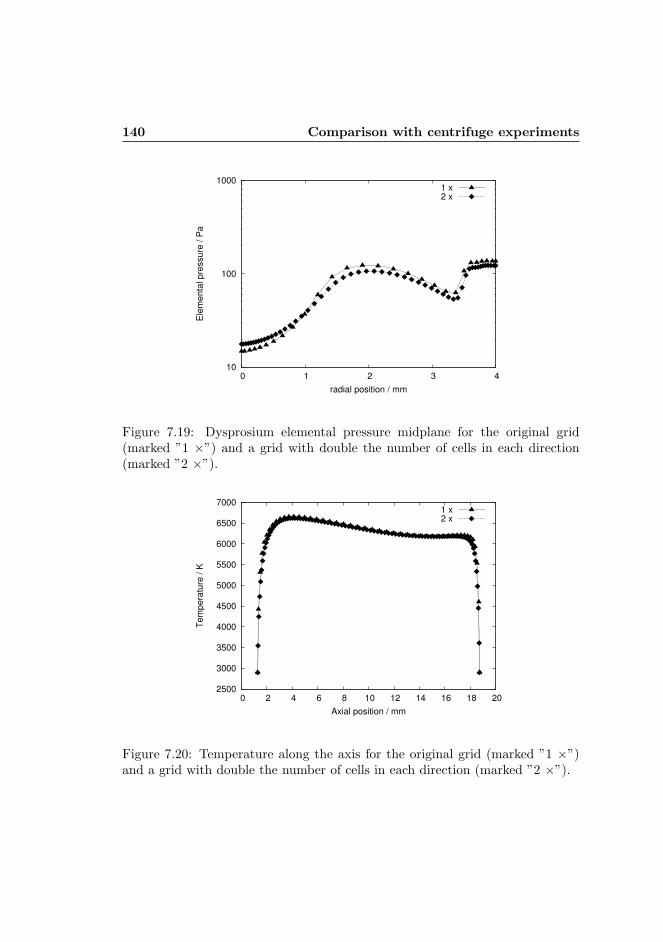
140 Comparison with centrifuge experiments
10
100
1000
0 1 2 3 4
Ele
menta
l pre
ssure
/ P
a
radial position / mm
1 x2 x
Figure 7.19: Dysprosium elemental pressure midplane for the original grid(marked ”1 ×”) and a grid with double the number of cells in each direction(marked ”2 ×”).
2500
3000
3500
4000
4500
5000
5500
6000
6500
7000
0 2 4 6 8 10 12 14 16 18 20
Tem
pera
ture
/ K
Axial position / mm
1 x2 x
Figure 7.20: Temperature along the axis for the original grid (marked ”1 ×”)and a grid with double the number of cells in each direction (marked ”2 ×”).

7.4 Cold spot vapour pressure 141
1000
2000
3000
4000
5000
6000
7000
0 1 2 3 4
Tem
pera
ture
/ K
radial position / mm
1 x2 x
Figure 7.21: Temperature midplane for the original grid (marked ”1 ×”) and agrid with double the number of cells in each direction (marked ”2 ×”).
resolve the large gradients near the bottom electrode resulting in overshoot andslightly lower values between 4 mm and 10 mm from the bottom electrode.A similar overshoot is witnessed in figure 7.19 where the coarse grid does notresolve the steep transition between atoms and molecules as well as the finergrid. The differences are small, however and do not alter the conclusions drawnin this chapter. The effect on the temperature is smaller yet, as shown in figures7.20 and 7.21 which show the temperature along the axis and midplane betweenthe electrodes, respectively.

142 Comparison with centrifuge experiments
7.5 Conclusions
A metal halide lamp with the COST geometry has been placed in a centrifugeto study the effect of the competition between convection and diffusion on thedistribution of additives in the lamp. Using the plasma modelling platformPlasimo, we have simulated the same lamp under different accelerational condi-tions. The density of dysprosium atoms in the ground state has been measuredusing the ilas technique for different lamp fillings and accelerational condi-tions. These ground state densities show good qualitative agreement with thedysprosium atom densities predicted by the model.
The quantitative agreement between the model and experiments are not asgood. One possible reason is the cold spot vapour pressure of the elements. Thiscold spot vapour pressure depends exponentially on the cold spot temperature.Increasing the temperature by 10 K is enough to raise the vapour pressure 30%.Using a vapour pressure of 150 Pa rather than the value of 517 Pa measured byX-Ray Fluorescence (XRF) by Nimalasuriya et al [21] on similar lamps yields abetter quantitative match between model and experiment.
The study with different vapour pressures also gives insight into the effectsof the radiation emitted by the dysprosium additives. Increasing the partialpressure of dysprosium atoms and ions increases the radiation emitted by thesespecies. Most of this radiation is emitted just off-centre from the axis. The ra-diative cooling by dysprosium causes the arc to contract. Increasing the amountof dysprosium in the discharge increases arc contraction.
The competition between convection and diffusion can be understood quan-titatively by introducing a Peclet number defined as the ratio between the rateof radial diffusion and axial convection. A Peclet number of unity leads to thegreatest axial segregation. Increasing the convection speed by increasing theacceleration changes the radial profiles from a step like profile to a more erraticprofile with local minima and maxima. Obtaining a homogeneous distributionof additives in the lamp can be achieved by designing a lamp such that thePeclet number is much greater or much smaller than unity.

Chapter 8
Convection in MH Lamps
8.1 Introduction
In earlier chapters the competition between convection and diffusion in metalhalide lamps was studied through numerical modelling. In chapter 4 a simplescaling law was found that can predict the conditions for which the lamp is moststrongly demixed. This simple scaling law relates the average segregation depthτ with the Peclet Pe number. The Peclet number is given by the ratio of theaxial convection and radial diffusion rates. In terms of the effective diffusioncoefficient of the element Dα and the axial convection speed Vz it is equal to:
Pe =R2Vz
LDα, (8.1)
with L the length and R the radius of the lamp. In this chapter a simplemodel will be derived to estimate Vz. This simple model will be compared withthe results of the more self-consistent numerical models presented in previouschapters.
8.2 A simple flow model
In this section a basic scaling law for the convection of metal halide lamps will bederived from the Navier Stokes equation and a greatly simplified energy balance.The approach is similar to Elenbaas [64], but with the emphasis on deriving an

144 Convection in MH Lamps
analytical expression. Elenbaas used a graphical method to get a more accurateestimation of the convection speed in high pressure mercury lamps.
Let us examine a cylinder with a large aspect ratio filled with an inert gas.The walls of the cylinder are held at a fixed temperature Tw. The effect of ohmicheating is modelled with a uniform heat source S. A schematic representationof the lamp is given in figure 8.1.
agρ
dp
dz
agρ
dp
dz
L
R
g
Figure 8.1: The simplified geometry used to examine convection in the lamp.The forces due to gravity and the pressure gradient on a volume element on theaxis and close to the walls are shown with arrows. Close to the walls the densityis greater and the net force is directed towards the bottom of the lamp. In thecentre the pressure gradient is identical but the density is much lower and thenet force is directed toward the top of the lamp.
The walls of MH lamps need to be relatively cool to avoid damage. For MHlamps with quartz walls this means a temperature of approximately 1200 K, ce-

8.2 A simple flow model 145
ramic MH lamps can sustain temperatures of 1500 K. The centre of the dischargemust be hot enough to excite the light emitting species and partially ionise thegas. In practice the temperature in the centre is approximately 6000 K.
The temperature difference between the hot centre and colder walls willcause a density difference, with the centre of the discharge being less dens thanthe gas near the wall. This density difference gives rise, under the influenceof gravity, to a buoyancy force. This buoyancy force, in turn, is balanced byviscous forces and drives the convection flow.
8.2.1 The temperature profile
In this subsection a simple approximation for the temperature profile is sought.The effects of radiation, chemistry and non uniform power input will be ig-nored in order to arrive at an analytical expression. Neglecting the influence ofconvection on the temperature balance one may write:
−1
r
∂
∂r
(
rλ∂T
∂r
)
= S,
where λ is the heat conductivity. As stated before, we assume the heat sourceS is uniform and independent of the temperature. Solving the equation underthe boundary conditions that T (R) = Tw and using r dT
dr
∣
∣
r=0= 0 yields:
T = Tw + T
(
1 −( r
R
)2)
, (8.2)
with T = SR2/4λ.
8.2.2 Velocity
The Navier Stokes equation for the gas in the cylinder is given by:
∂ρ~u
∂t+ (ρ~u · ∇) ~u = −∇p + ∇ · (µ∇~u) + ρ~ag, (8.3)
with ρ the density, ~u the velocity, t the time, p the pressure, µ the dynamicviscosity and ~ag the gravitational acceleration.
As the aspect ratio of the cylinder is large, a number of simplifications arepossible. Away from the ends, the temperature depends solely on the radialposition (T = T (r)). The velocity through the midplane is axially directed andalso solely radially dependent ( ~u = u(r)~ez). The time dependency is ignored

146 Convection in MH Lamps
as we are looking for a stationary solution. It is also assumed that the viscousforces are much larger than the inertial forces (the Reynolds number is low). Tofurther simplify the equations constant viscosity is assumed.
Using the above simplifications the Navier Stokes equation reduces to:
∂p
∂z=
1
r
∂
∂r
(
µr∂u
∂r
)
− ρag, (8.4)
∂p
∂r= 0 and (8.5)
∂p
∂φ= 0. (8.6)
The equation above shows that the pressure is independent of the radial andazimuthal position. If the aspect ratio is large enough, the pressure gradientwill also be independent of the axial position.
The equation above is made dimensionless by introducing a dimensionlessposition x = r/R, the dimensionless density ρ∗ = ρ/ρ0, with ρ0 the density inthe centre, and the dimensionless velocity u∗ given by
u∗ =µ
ρ0agR2u. (8.7)
Equation (8.4) then becomes
1
x
d
dx
(
xdu∗
dx
)
= ρ∗ + A, (8.8)
with A the dimensionless pressure gradient,
A =1
ρ0ag
dp
dz. (8.9)
By integration we obtain:
xdu∗
dx=
∫ x
0
ρ∗x′dx′ +1
2Ax2 + C1,
with C1 = 0 since xdu∗
dx = 0 for x = 0. Integrating a second time yields:
u∗(x) =
∫ x
0
1
x′
(
∫ x′
0
x′′ρ∗dx′′
)
dx′ +1
4Ax2 + u0, (8.10)
with u0 the convection speed on the axis to be determined by the boundaryconditions. As the lamp is closed the net flux through the midplane must be
zero (∫ R
0ρ(r)u(r)rdr = 0). This condition will be used to find the parameter A.

8.2 A simple flow model 147
Substitution of the temperature profile
With the temperature profile found in the previous section one can now evaluatethe integral in equation (8.10). With the use of the ideal gas law and 8.2 onemay obtain:
ρ∗ =(
1 − x2T /T0
)−1
, (8.11)
with T0 the temperature on the axis. Substitution into (8.10) results in:
u∗(x) = u0 +1
4Ax2 + Li2
(
(T /T0)x2)
, (8.12)
with Li2(x) the dilogarithm:
Li2(x) =
∫ 0
x
ln(1 − y)
ydy. (8.13)
Using the no-slip condition on the wall (u∗(1) = 0) one may derive:
u∗(x) =1
4A(x2 − 1) + Li2
(
(T /T0)x2)
− Li2
(
T /T0
)
. (8.14)
To obtain the value of A that satisfies∫ R
0ρ(r)u(r)rdr = 0 a numerical technique
is required. Using the Levenberg-Marquand algorithm the value for A has beencalculated for different ratios of T /T0. The result is shown in figure 8.2. Atypical MH lamp has a ratio T /T0 between 0.7 and 0.8 resulting in a value ofA ≈ −20. From this result the dimensionless velocity u∗(x) may be calculated.An example is shown in figure 8.3. Note that this dimensionless velocity dependsonly on the ratio T /T0.
8.2.3 Comparison with grand numerical model results
The velocity predicted by the simple flow model with a near analytical resultmay now be compared with the more complex, two dimensional model with anon-constant viscosity. Such a comparison is shown in figure 8.4, for a lampwith a mercury pressure of 10 bar, a central temperature of 6000 K, and a walltemperature of 1200 K. In the numerical model the viscosity has been calculatedby Wilke’s formula [36]. For comparison, a viscosity of 4 × 10⁻⁴Pas has beenchosen in the analytical expression. The velocity predicted by the analyticalexpression is greater in magnitude than that predicted by the more complexnumerical model. The profile is remarkably similar, however.

148 Convection in MH Lamps
-25
-20
-15
-10
-5
0
0 0.1 0.2 0.3 0.4 0.5 0.6 0.7 0.8 0.9
A
T /T0
Figure 8.2: Value of A so that the equation∫ R
0ρ(r)u(r)rdr = 0 is satisfied.
Typical MH lamps have a ratio T /T0 between 0.7 and 0.8.
To obtain an analytical expression a constant viscosity has been assumed.The viscosity is, however, anything but constant, as is shown in figure 8.5.Furthermore, an infinite aspect ratio has been assumed. In reality the aspectratio of the lamp under study is only 5. To get a better estimate the non-constant viscosity needs to be taken into account. To correct for the smalleraspect ratios a two dimensional model is required. In either case, the convectionflow can only be solved numerically.
We may, however, use the scaling parameter in (8.7) to find a scaling lawfor discharges with a similar temperature profile. The dimensionless velocityu∗ only depends on the ratio T /T0. For discharges with the same temperatureprofile we have:
u ∝ρ0agR
2
µ. (8.15)
Thus the velocity is
• proportional to the square of the radius,

8.2 A simple flow model 149
-0.04
-0.02
0
0.02
0.04
0.06
0.08
0.1
0.12
0.14
0.16
0 0.2 0.4 0.6 0.8 1
u*
x
Figure 8.3: The dimensionless velocity u∗ for T /T0 = 0.8.
• proportional to the density at the centre,
• proportional to the gravitational acceleration and
• inversely proportional to the viscosity.
Using the ideal gas law one may rewrite this as
u ∝mHgpagR
2
µkT0, (8.16)
with mHg the mass of the mercury atom. Thus the velocity also increases lin-early with the total pressure. In the next two sections the validity of thesescaling laws will be examined using the results from more complex numericalmodels. In particular the dependance an the pressure, the radius and the grav-itational acceleration are examined.

150 Convection in MH Lamps
-0.1
-0.05
0
0.05
0.1
0.15
0.2
0.25
0 1 2 3 4
ve
locity /
(m
/s)
radial position / mm
analytical resultnumerical model result
Figure 8.4: Axial velocity as calculated from (8.10) compared with results fromthe MH lamp model. To get the velocity from the analytical model a value of4 × 10−4Pas has been chosen for the viscosity.
8.3 Mercury lamp
The additives in MH lamps significantly improve the colour rendering of thesedevices as compared with lamps containing pure mercury. The impact on theconvection patterns is much smaller and indirect. We examine the convectionwith numerical experiments of a lamp containing pure mercury. The model ofthis lamp is identical to the model for the mercury lamp described in chapter4. The total pressure is varied by increasing the lamp filling.
Equation (8.16) predicts a linear relationship between the velocity and thepressure. The assumptions of a uniform power input is not valid in lamps ofthis type as most of the power is deposited on the axis close to the electrodes.The viscosity and thermal conductivity are also temperature dependent. Thetemperature profiles are also effected by the pressure. Nevertheless, as figure

8.3 Mercury lamp 151
0.0002
0.0003
0.0004
0.0005
0 0.001 0.002 0.003 0.004
vis
co
sity
/ (P
a s
)
radial position / m
Figure 8.5: Viscosity from the MH lamp model calculated by the Wilke formula[36].
8.6 shows, the velocity does show a linear dependence on the pressure.
The dependence on the square of the radius has also been investigated byexamining two lamps with the same volume and input power but with twodifferent radii: 2 mm and 4 mm respectively (with lengths of 80 mm and 20 mm).According to (8.16) the velocity should increase with the square of the radius.The dimensionless velocity u∗ should be independent of the radius and the totallamp pressure. Figure 8.7 shows the dimensionless velocity midplane on theaxis as a function of the pressure for models of lamps with a radius of 2 mmand 4 mm compared. The lamp with the longer aspect ratio has a greaterdimensionless velocity. There is also a weak dependence on the pressure.

152 Convection in MH Lamps
0
0.05
0.1
0.15
0.2
0.25
0.3
0.35
0.4
0.45
0.5
0 1 2 3 4 5 6
ve
locity /
(m
/s)
Pressure /MPa
Figure 8.6: The axial velocity on the axis halfway between the electrodes in apure mercury lamp for different pressures corresponding to lamp fillings between3 mg and 60 mg.
8.4 Metal halide lamp
We examined the velocity on the axis halfway between the electrodes as calcu-lated by the metal halide lamp model in chapter 7. To compare with results ofexperiments in a centrifuge we used different values for ag ranging from 1 g to10 g. The model was also run with different lamp fillings from 3 mg to 20 mg.The simple flow model derived earlier predicts a linear dependence on the prod-uct of the pressure and the acceleration ag. Figure 8.8 shows that such a lineardependence is a good approximation. This in spite of the non-constant powerinput, changing temperature profiles for different pressures and the dependenceof the viscosity and thermal conductivity on the temperature.

8.5 Conclusion and discussion 153
0.04
0.05
0.06
0.07
0.08
0.09
0 1 2 3 4 5 6
u*
pressure / MPa
2 mm
4 mm
Figure 8.7: The dimensionless axial velocity in a pure mercury lamp. Resultsare shown for different pressures corresponding to lamp fillings between 3 mgand 60 mg and lamp radius of 2 mm and 4 mm compared. According to (8.16)one would expect a single horizontal line in this graph.
8.5 Conclusion and discussion
A simple semi-analytical expression has been derived for the axial velocity ina metal halide lamp. The derivation is not completely analytical as one ofthe parameters needs to be determined numerically. This numerical procedurehowever, is much less time-consuming than the full numerical models consistingof many coupled non-linear differential equations, ray-tracing and the determi-nation of the chemical equilibrium via Gibbs minimisation. Furthermore, thisparameter A, representing the dimensionless pressure gradient, depends onlyon the temperature difference between the centre and the wall of the discharge.Comparing the velocity with full numerical model results shows, however, thatit gives only a rough approximation of the axial velocity.

154 Convection in MH Lamps
0
0.1
0.2
0.3
0.4
0.5
0.6
0.7
0.8
0.9
1
0 1 2 3 4 5 6 7 8 9 10
ve
locity /
(m
/s)
pressure*acceleration / (MPa*g)
Axial velocity midplane, on the axis
3 mg 5 mg 7 mg 10 mg
Figure 8.8: The axial velocity on the axis halfway between the electrodes fordifferent lamp fillings under different accelerational conditions.
The scaling law derived is more useful, it shows a linear dependence of theaxial velocity on the pressure. Looking at the results from numerical modelsof a pure high pressure mercury lamp and a metal halide lamp shows thatthis is indeed a good approximation. The dependence on the gravitationalacceleration has also been examined. This is of interest for the estimation ofthe axial velocity in experiments conducted in a centrifuge, such as those inchapter 7. Results from the metal halide lamp modelled in this chapter showthat the predicted linear relationship between the gravitational acceleration andthe axial convection holds to good approximation. The scaling law also predictsthat the velocity is proportional to the square of the radius of the discharge. Thisscaling law does not hold if the aspect ratio is also changed, as demonstratedby a numerical model of a pure mercury discharge.

Chapter 9
General conclusion
The plasma simulation platform plasimo has been used to develop a numericalmodel of the additive distribution in vertically burning metal halide lamps. Themodel assumes axial symmetry, a steady laminar flow and the presence of LTE.Two different transport modes were used. The balances of mass, momentumand energy and the conservation of elements were solved using the control vol-ume approach, the radiation transport is treated by means of ray tracing. Theinput of this model is the set of control parameters, such as the fill chemistry,driving power and vessel shape. The output is formed by plasma properties;such as the voltage over the lamp electrodes, the production of heat and theemission of radiation. Along the way many more plasma properties are cal-culated: the distribution of the elements over the lamp and the fields of thetemperature, the velocities and the pressure. The model attempts to calculatethese parameters in a self consistent manner from first principles. There is noplace for fudge parameters. At the same time the model must be as simple aspossible; approximations that can be made should be made.
Using this model numerical simulations have been performed of lamps con-taining mercury with sodium iodide and dysprosium iodide (Na and Dy lamps).Initial studies were carried with Na as the simulation of the Na lamps is rel-atively easy. The chemistry is rather simple and only a few Na lines have tobe taken into account in the ray tracing procedure. The modelling of the Dylamp is more complicated; a proper chemical description needs to include morespecies and an enormous number of radiative transitions have to be dealt with.There was no choice, however; we had to construct a model for the Dy lampsince the experimental validation of a Na lamp is not easy.

156 General conclusion
The central aim of the numerical studies was to come to a basic understand-ing of the transport of additives in MH lamps. To this end model calculationswere done for many different conditions, that is to say, for different pressures,accelerations and chemical compositions. Additionally, the studies were carriedout on the influence of the cold spot vapour pressure, the elastic scatteringcross section between dysprosium ions and mercury atoms and the choice ofdata set for the transition probabilities of dysprosium atoms and ions. Resultsfrom these calculations were classified by looking at the output; in particular atthe distribution of additives, the temperature, the velocity and the density ofthe radiative species. The main results can be classified by the introduction oftwo dimensionless parameters: the segregation depth of the lamp τ and the Penumber. Together these describe the axial segregation in the lamp.
9.1 Axial segregation
Axial segregation was shown to be the result of the competition between ax-ial convection and radial diffusion. This competition is best expressed by thedimensionless Peclet number. When the Peclet number is approximately equalto unity axial segregation is strongest. The degree of axial segregation is bestexpressed by the dimensionless segregation depth τ . The largest value of τ de-pends on the element under study and on the position in the discharge wherethe molecules dissociate to form ions. This position, in turn, depends on thetemperature profile and on the dissociation energy of the molecule.
The Peclet number depends on the diffusion coefficient, the lamp geometryand the axial convection speed. The diffusion coefficient can be estimated fromthe total lamp pressure and the elastic cross sections of the additives with thebackground mercury gas. In chapter 8 a scaling law was derived for the depen-dence of the convection on the pressure and (in the case of a centrifuge) on theaccelerational conditions. It was shown that the convection depends linearly onthe pressure and the acceleration. The convection speed also depends on thedensity gradients, and is thereby related to the temperature profile.
9.2 Temperature profile
In chapter 4 it was found that adding dysprosium to the discharge causes thetemperature profile to contract. The temperature along the flanks is decreased,when compared to a pure mercury discharge, by radiation from dysprosium

9.3 Comparison with experiments 157
atoms. To still allow the same ohmic dissipation the temperature along theaxis has to increase. This arc contraction is in agreement with experimentalresults found in X-Ray absorption measurements [65]. In chapter 5 it was foundthat the degree of contraction predicted by the model depends on the choiceof data set for the transition probabilities. In chapter 7 it was also found thatthe cold spot vapour pressure directly influences the degree of contraction. Thesodium discharges have a lower temperature along the axis due to the lowerionisation potential. Additionally, sodium has a number of optically thick lineswhich heat up the edges of the discharge. Dysprosium has a spectral grass fieldof lines, most of which are optically open. In chapter 5 it was found that, forthe purpose of calculating the temperature profile, the spectral grass field canbe approximated by two effective transitions.
9.3 Comparison with experiments
The results of the model for the Dy lamp were compared to that of experi-ments. In chapter 6 we dealt with microgravity conditions whereas chapter 7was devoted to lamps in a centrifuge. Both studies show that the model iscapable to predict main trends. However, precise quantitative agreement canonly be obtained if experimental techniques are available that make it possibleto determine the cold spot temperature with high precision. This temperatureis very important in the determination of the vapour pressure of the Dy con-taining molecules above the salt pool and thus for the number of Dy containingcomponents that enter the plasma phase.
Better input data is also needed for the elastic scattering cross sections be-tween the Dy containing species and the mercury atoms which vastly outnumberall other species. In chapter 6 the influence of the choice of elastic scatteringcross sections between dysprosium ions and the background mercury gas wasstudied. The ratios of dysprosium to mercury ions in the centre of the dischargeappeared particularly sensitive to the choice of cross section. Thus, measuringthis ratio could help to validate elastic scattering cross section data. The mea-surements would have to be performed in lamps with low convection speeds. Alow cost alternative to taking lamps to the international space station wouldbe to use lamps with a long aspect ratio and relatively small mercury dosings(approximately 5 mg for a lamp equal in volume to the cost reference lamp).As is shown in chapter 8 such conditions would also lead to low Peclet numbers.

158 General conclusion
9.4 Outlook
To keep both the model and the experiments as simple as possible only lampswith a single salt additive have been considered. Commercial lamps typicallyhave more additives. The model that has been developed alows for more thanone salt additive, however. The number of additives is limited only by theamount of computer memory required for the look-up table with the speciesdensities as a function of the elemental abundance, temperature and pressure.Currently, these lookup tables are around 28 MiB in size. Adding one or twomore additives lies well within the possibilities. Adding as many as six differentadditives to fully simulate the mixture in a commercial lamp would require anoverhaul of the look-up tables from the current linear interpolation scheme toa smarter interpolation scheme. Studying mixtures with two or three additiveswould also be of interest to study the effect of additives on each other.
A related topic that is of utmost interest is how the combination of radia-tive cooling and the association/dissociation position will facilitates instabilities.Due to radiative contraction the wall stabilisation will be lost. Moreover self-generated magnetic fields might be able to excite helical instabilities. The he-lical instabilities would require a full three-dimensional time dependent model.Other types of instabilities that can be present are those initiated by acousticresonances. These also require a time dependent model. There are certainlyplenty of challenges left in the study of metal halide lamps.

Bibliography
[1] M. Gendre. Two centuries of electric light source innovations. availableonline: http://www.einlightred.tue.nl/lightsources/history/.
[2] P. Flesch, editor. Light and Light Sources, High-Intensity Discharge Lamps.Springer, Berlin, 2006.
[3] C. P. Steinmetz. Us patent no. 1025932 means for producing light, 1902.
[4] A. D. Jackson, III R. G. Gibson, S. A. Carleton, S. Wu, L. N. Kowalczyk,T. Steere J. J. Palmer, J. C. Alderman, Sr. J. E. Conrad, and K. L. Collins.United states patent 6833677 150w-1000w mastercolor ceramic metal halidelamp series with color, 2004.
[5] E. Fisher. Axial segregation of additives in mercury-metal-halide arcs. J.Appl. Phys., 47:2954, 1975.
[6] D. E. Work. Chemistry of metal halide lamps: a review. Light. Res. Tech.,13:143, 1987.
[7] J. T. Dakin, Jr. T. H. Rautenberg, and E. M. Goldfield. Anatomy of avertical metal halide discharge. J. Appl. Phys., 66:4074–4088, 1989.
[8] R. J. Zollweg. Reducing additive segregation in metal halide high-intensitydischarge lamps. J.I.E.S, 4:12–18, 1975.
[9] W. W. Stoffels, A. H. F. M. Baede, J. J. A. M. van der Mullen, M. Haverlag,and G. Zissis. Definition of a high intensity metal halide discharge referencelamp. Meas. Sci. Technol., 17:N67–N70, 2006.
[10] M. Kaning, B. Schalk, and H. Schneidenbach. Experimental determinationof parameters for molecular continuum radiation of rare-earth iodides. J.Phys. D: Appl. Phys.”, 40:3815–3822, 2007.

160 BIBLIOGRAPHY
[11] T. Nimalasuriya, N. B. M. Pupat, A. J. Flikweert, W. W. Stoffels,M. Haverlag, and J. J. A. M. van der Mullen. Optical emission spec-troscopy of metal-halide lamps: Radially resolved atomic state distributionfunctions of dy and hg. Journal of Applied Physics, 99:053302, 2006.
[12] T. Nimalasuriya, A. J. Flikweert, M. Haverlag, P. C. M. Kemps, G. M. W.Kroesen, W. W. Stoffels, and J. J. A. M. van der Mullen. Metal halidelamps in the international space station ISS. J. Phys. D, 39:2993–3001,2006.
[13] A. J. Flikweert, T. Nimalasuriya, G. M. W. Kroesen, and W. W. Stof-fels. Imaging laser absorption spectroscopy of the metal-halide lamp in acentrifuge (1-10g). Plasma Sources Sci. Technol., 16:606–613, 2007.
[14] T. Nimalasuriya, M. L. Beks, A. J. Flikweert, W. W. Stoffels, M. Haverlag,and J. J. A. M. van der Mullen. Metal-halide lamps in micro-gravity,experiment and model. J. Phys. D: Appl. Phys.”, 2007. submitted.
[15] S. V. Patankar, editor. Numerical Heat Transfer and Fluid Flow. NewYork: McGraw-Hill, 1980.
[16] http://plasimo.phys.tue.nl/.
[17] M. S. Benilov and M. D. Cunha. Bifurcation points in the theory of axiallysymmetric arc cathodes. Phys. Rev. E., 68(5):056407, Nov 2003.
[18] M. S. Benilov, M. D. Cunha, and G. V. Naidis. Modelling current transferto cathodes in metal halide plasmas. J. Phys. D: Appl. Phys.”, 38:3155–3162, 2005.
[19] T. Nimalasuriya, J. J. Curry, C. J. Sansonetti, E. J. Ridderhof, A. J. Flik-weert, W. W. Stoffels, M. Haverlag, and J. J. A. M. van der Mullen. X-rayinduced fluorescence measurement of the density distribution of Dy and Hgin a metal-halide lamp. XXVIIth International Conference on Phenomenain Ionized Gases, 2005.
[20] T. Nimalasuriya, G. M. Thube, A. J. Flikweert, M. Haverlag, G. M. W.Kroesen, W. W. Stoffels, and J. J. A. M. van der Mullen. Axial segregationin metal-halide lamps under varying gravity conditions ranging from 1 to10 g. J. Phys. D, 40:2839–2846, 2007.

BIBLIOGRAPHY 161
[21] T. Nimalasuriya, J. J. Curry, C. J .Sansonetti, E. J. Ridderhof, S. D. Shas-tri, A. J. Flikweert, W. W. Stoffels, M. Haverlag, and J. J. A. M. van derMullen. X-ray induced fluorescence measurement of segregation in a dyi3-hg metal-halide lamp. J. Phys. D, 40:2831, 2007.
[22] A. J. Flikweert, M. van Kemenade, T. Nimalasuriya, M. Haverlag, G. M. W.Kroesen, and W. W. Stoffels. Axial segregation in metal halide lampsunder varying conditions during parabolic flights. J. Phys. D: Appl. Phys.”,39:1599–1605, 2006.
[23] D. A. Larson, H. D. Fraser, W. V. Cushing, and M. C. Unglert. Higherefficiency light source through use of additives to mercury discharge. Illu-minating Engineering, 58:434, 1963.
[24] M. Sugiura. Review of metal-halide discharge-lamp development 1980-1992.Science, Measurement and Technology, IEE Proceedings A, 140:443–449,1993.
[25] G. G. Lister, J. E. Lawler, W. P. Lapatovich, and V. A. Godyak. Thephysics of discharge lamps. Rev. Mod. Physics, 76:542–598, 2004.
[26] S. Hashiguchi, K. Hatase, S. Mori, and Tachibana. Numerical simulationof metal-halide lamp using a time-dependent two-dimensional model. J.Appl. Phys., 92:45–53, 2002.
[27] D.A. Benoy. Modelling of thermal argon plasmas. PhD thesis, EindhovenUniversity of Technology, The Netherlands, 1993.
[28] J. van Dijk. Modelling of Plasma Light Sources — an object-oriented ap-proach. PhD thesis, Eindhoven University of Technology, The Netherlands,2001.
[29] S. Chapman and T. G. Cowling, editors. The Mathematical Theory ofNon-Uniform Gases, 3rd ed. Cambridge University Press, 1974.
[30] J. O. Hirschfelder, C. F. Curtiss, and R. B. Bird, editors. Molecular Theoryof Gases and Liquids. (New York: Wiley & Sons), 1964.
[31] H. van der Heijden. Modelling of Radiative Transfer in Light Sources. PhDthesis, Eindhoven University of Technology, The Netherlands, 2003.

162 BIBLIOGRAPHY
[32] A. Hartgers, H. W. P. van der Heijden, M. L. Beks, J. van Dijk, and J. A. M.van der Mullen. An elemental diffusion description for LTE plasma models.J. Phys. D: Appl. Phys., 38(18):3422–3429, 2005.
[33] M. Mitchner and C. H. Kruger, editors. Partially Ionized Gases. (NewYork: Wiley & Sons), 1973.
[34] C. W. Johnston. Transport and equilibrium in molecular plasmas - thesulfur lamp. PhD thesis, Eindhoven University of Technology, The Nether-lands, 2003.
[35] J. N. Butler and R. S. Brokaw. Thermal conductivity of gas mixtures inchemical equilibrium. J. Chem. Phys., 26(6):1636, 1956.
[36] C. R. Wilke. A viscosity equation for gas mixtures. J. Chem. Phys., 18:517–519, 1950.
[37] S. Paolucci. The differentially heated cavity. Sadhana, 19:619–647, 1994.
[38] H. G. Hulsman and J. Mentel. The helical magnetic instability of arcs inan axial magnetic field treated by a linear time dependent theory. Phys.Fluids, 30:2266–2273, 1987.
[39] W. W. Stoffels, F. van den Hout, G. M. W. Kroesen, M. Haverlag, andR. Keiser. Helical instabilities in metal halide lamps under micro andhyper-gravity conditions. App. Phys. Lett., 88:091502, 2006.
[40] M. L. Beks, A. Hartgers, and J. J. A. M. van der Mullen. Demixing ina metal halide lamp, results from modelling. J. Phys. D: Appl. Phys.,39:4407, 2006.
[41] H. van der Heijden and J. J. A. M. van der Mullen. General treatment of theinterplay between fluid and radiative transport phenomena in symmetricplasmas: the sulfur lamp as a case study. J. Phys. D: Appl. Phys.”, 35:2112–2125, 2002.
[42] C. W. Johnston, H. van der Heijden, G. Janssen, J. van Dijk, and J.A.M.van der Mullen. A self consistent lte model of microwave driven high pres-sure sulfur lamp. J. Phys. D: Appl. Phys.”, 35:342–351, 2002.
[43] Private communications a.h.f.m. baede.

BIBLIOGRAPHY 163
[44] M. E. Wickliffe, J. E. Lawler, and G. Nave. Atomic transition probabilitiesfor dy i and dy ii. J. Quant. Spectrosc. Radiat. Trans., 66:363–404, 2000.
[45] W. G. Vincenti and C. H. Kruger Jr. Introduction to Physical Gas Dynam-ics. John Wiley and Sons, Inc., 1965.
[46] M. Censkya, L. Hnedkovskya, and V. Majerb. Heat capacities of aqueouspolar aromatic compounds over a wide range of conditions. part i: phe-nol, cresols, aniline, and toluidines. Journal of Chemical Thermodynamics,37:205–219, 2005.
[47] W. R. Smith and R. W. Missen. Chemical Reaction Equilibrium Analysis:Theory and Algorithms. Krieger publishing company, 1991.
[48] C. W. Bale, P. Chartrand, S. A. Degterov, G. Eriksson, K. Hack, R. BenMahfoud, J. Meloncon, A. D.Pelton, and S. Peterson. calphad, 26:189–228, 2002.
[49] http://gttserv.lth.rwth-aachen.de/ cg/software/chemapp/cal-doc/cal84.html.
[50] S. Chandrasekhar. Radiative transfer. Dover Publications Inc. New York,1960. Revised edition.
[51] N. V. Gorschkov, V. A. Komarovski, A. L. Osherovich, N. P.Penkin, and R. Khefferlin. Opt. Spectrosc., 48:362–4, 1980.data availabe online from the Harvard Smithsonian Centerfor Astrophysics Kurucz Atomic Line Database http://cfa-www.harvard.edu/amdata/ampdata/kurucz23/sekur.html.
[52] J. Waymouth. Electric discharge lamps. MIT press, Cambridge, 1971.
[53] J. R. Coaton and A. M. Marsden. Lamps and Lighting 4th edition. Arnold,London, 1997.
[54] X. Zhu. Active spectroscopy on HID lamps, Exploration of various methods.PhD thesis, Eindhoven University of Technology, The Netherlands, 2005.
[55] A. J. Flikweert, T. Nimalasuriya, C. H. J. M. Groothuis, G. M. W. Kroesen,and W. W. Stoffels. Axial segregation in high intensity discharge lampsmeasured by laser absorption spectroscopy. Journal of Applied Physics,98:073301, 2005.

164 BIBLIOGRAPHY
[56] M. L. Beks, J. van Dijk, A. Hartgers, and J. J. A. M. van der Mullen. Astudy on the effects of geometry on demixing in metal halide lamps. IEEETransactions on Plasma Science, Volume: 35:1335–1340, 2007.
[57] S. D. Rockwood. Phys. Rev. A, 8:2348–58, 1973.
[58] C. L. Chen and M. Raether. Phys. Rev., 128:2679, 1962.
[59] J. J. A. M. van der Mullen. Phys. Rep., 191:109, 1990.
[60] J. de Groot and J. van Vliet, editors. The high pressure sodium lamp.Philips technical library, kluwer technische boeken, Deventer, Antwerpen,1986.
[61] W. W. Stoffels, P. C. M. Kemps, J. Beckers, G. M. W. Kroesen, andM. Haverlag. Light emission of metal halide lamps under micro- and hy-pergravity conditions. Appl. Phys. Lett., 87:241501, 2005.
[62] W. W. Stoffels, A. J. Flikweert, T. Nimalasuriya, J. J. A. M. van derMullen, G. M. W. Kroesen, and M. Haverlag. Metal Halide Lamps: grav-itational influence on color separation. Pure Appl. Chem., 78:1239–1252,2006.
[63] M. van Kemenade. Axial segregation in high intensity discharge lamps.Master’s thesis, Eindhoven University of Technology, 2004.
[64] W. Elenbaas, editor. The High Presure Mercury Vapour Discharge. NorthHolland Publishing Company, Amsterdam, 1951.
[65] T. Nimalasuriya et al. to be submitted. J. Phys. D: Appl. Phys.”, 2008.

Dankwoord
Bijna zes jaar geleden kwam ik bij Eddie van Veldhuizen op de kamer op zoeknaar een afstudeeropdracht. Deze bracht mij in contact met Joost van derMullen die mij verder introduceerde bij de groep EPG (Elementaire Processenin Gasontladingen) en het Plasimo team. Tijdens mijn afstuderen vroeg Joostvan der Mullen of ik wou blijven om te promoveren. Dit wou ik, en na mijnafstuderen ging ik gelijk aan de slag. Niet aan lage druk extreem ultravioletbronnen zoals tijdens mijn afstudeeronderzoek maar aan een lampje dat gewoonzichtbaar licht uitstraalt. Dat met een lampje interessante wetenschap valt tebedrijven heb ik de afgelopen vier jaar wel ondervonden. Ik dank dan ook mijnpromotor en begeleider Joost van der Mullen van harte voor de ondersteuningen de inspiratie die nodig waren om tot dit proefschrift te komen.
Dat lampjes een interessant onderwerp voor wetenschappelijk onderzoek zijnwas natuurlijk al langer bekent bij mijn tweede promotor: Marco Haverlag. Ikben dan ook dankbaar voor zijn hulp en de discussies die ik met hem gevoerdheb. Ook wil ik mijn overige commissieleden bedanken voor hun nuttige bijdra-gen en correcties aan het proefschrift.
De numerieke modellen in dit proefschrift maken gebruik van het Plasimoplatform, oorspronkelijk geschreven door Dany Benoy. Door vele bijdragen vanafstudeerders en promovendi is deze code van een plasma simulatie model mettwee toepassingen geevolueerd in een simulatie platform met vele mogelijke toe-passingen op plasma gebied. Ik ben daarbij in het bijzonder Jan van Dijk, Harmvan der Heijden en Bart Hartgers dank verschuldigd. Jan van Dijk voor de alge-mene ondersteuning en ontwikkeling van Plasimo en Harm van der Heijden enBart Hartgers voor de stralingscode. Bart Hartgers is ook in het begin stadiumvan mijn onderzoek zeer behulpzaam geweest in het aan de praat krijgen vanmodellen. Verder dank ik mijn voormalige kamer-genoot Bart Broks voor denuttige discussies en Tanya Nimalasuriya en Arjan Flikweert voor de prettigesamenwerking, met name in het tot stand komen van hoofdstukken 6 en 7. Ten-

166 BIBLIOGRAPHY
slotte wil bedank ik mijn vriendin Kim Peerenboom voor het nakijken van mijnproefschrift en het geduld met mij in de weken voor mijn promotie.

Curriculum VitaeBorn October 2nd 1975 in Bellingwolde
Education
1992-1994 International Baccalaureate. First year at the International School of Kenyain Nairobi, Kenya second year at Rijnland’s Lyceum in Oegstgeest, The Nether-lands.
1994-2003 Master of Applied Physics at the Eindhoven University of Technology.
2004-2008 Ph.D. research in numerical plasma physics at the Eindhoven University ofTechnology.
Traineeships
April 1996 - December 1996 Internship with the Low Temperature Physics group ofthe faculty of applied physics under supervision of prof. dr. A. T. A. M. de Waeleand ir. R.M.S. Knops. Title of the report: ”Turbulentie bij een diameterovergangin de resonator van een thermo-akoestische koeler.”
September 1999 - May 2000 Trainee with Fymaz and FEV in Aken (Germany). Un-der supervision of dr. ir. A.P.J. Voncken and dr. H.J.H. Clercx. Title of the report”Modeling Dynamically Loaded Cylindrical Bearings”
September 2002 - December 2003 Masters thesis at the group EPG of the facultyof applied physics (TUE). Supervisors: Dr. J.J.A.M. van der Mullen, ir. B.H.P.Broks and ir. W.J.M. Brok . Title of the report ”Towards a Hybrid Fluid-MonteCarlo Model for Pulsed Hollow Cathode Discharges”.
Experience
December 1996 - March 1998 Student tutor assisting with a practical class for me-chanical engineering.
July 2000-July 2002 Modelling of the dynamic behaviour of electro magnetic valvesfor Fymaz in Stolberg (Germany).