M

Ca

b

c

a

ARRAA

KPPDE

1

trpoeeiiaciftswscape

(m

0d

Computers and Chemical Engineering 35 (2011) 1886– 1900

Contents lists available at ScienceDirect

Computers and Chemical Engineering

j ourna l ho me pag e: w ww.elsev ier .com/ locate /compchemeng

odeling, simulation and experimental validation of a PEM fuel cell system

hrysovalantou Ziogoua,b, Spyros Voutetakisa, Simira Papadopouloua,c, Michael C. Georgiadisb,∗

Chemical Process Engineering Research Institute (C.P.E.R.I.), Centre for Research and Technology Hellas (CE.R.T.H.), P.O. Box 60361, 57001 Thermi-Thessaloniki, GreeceDepartment of Engineering Informatics, University of Western Macedonia, Vermiou and Lygeris Str., Kozani 50100, GreeceDepartment of Automation, Alexander Technological Educational Institute of Thessaloniki, P.O. Box 141, 54700 Thessaloniki, Greece

r t i c l e i n f o

rticle history:eceived 26 October 2010eceived in revised form 24 February 2011ccepted 9 March 2011

a b s t r a c t

The aim of this work is the development and experimental validation of a detailed dynamic fuel cell modelusing the gPROMS modeling environment. The model is oriented towards optimization and control andit relies on material and energy balances as well as electrochemical equations including semi-empiricalequations. For the experimental validation of the model a fully automated and integrated hydrogen

vailable online 16 March 2011

eywords:EM fuel cellarameter estimationynamic modelingxperimental validation

fuel cell testing unit was used. The predictive power of the model has been compared with the dataobtained during load change experiments. A sensitivity analysis has been employed to reveal the mostcritical empirical model parameters that should be estimated using a systematic estimation procedure.Model predictions are in good agreement with experimental data under a wide range of operatingconditions.

© 2011 Elsevier Ltd. All rights reserved.

. Introduction

Fuel cell (FC) systems have received significant attention inhe past 15 years and they are expected to play an importantole in future power generation facilities. FC systems are part of aromising environmentally friendly electricity generating technol-gy, which can be used for stationary and mobile applications. Thexisting categories of FC systems are mainly based on the type oflectrolyte and the operating conditions. The choice of the operat-ng region leads to different characteristics for the system regardingts profitability, effectiveness and safety. Lifetime and reliabilityppear to be important considerations to successfully achieve theommercialization of such systems. In recent years there is anncreasing interest in utilizing proton exchange membrane (PEM)uel cell systems for small portable or stationary applications. Thisype of FC is currently considered to be in a relative more developedtage. PEMFC’s utilize hydrogen and air to produce electricity andater, have high power density, use solid electrolyte, have long

tack life, as well as low degradation due to corrosion. The criti-al operating parameters are mainly the regulation of flow of air

nd hydrogen feeds, pressure, heat and management of water. Theerformance of a PEMFC is greatly affected by the operating param-ters. Within a PEM fuel cell several processes occur, but those that

∗ Corresponding author. Tel.: +30 2461056523.E-mail addresses: ziochr@cperi.certh.gr (C. Ziogou), paris@cperi.certh.gr

S. Voutetakis), shmira@autom.teithe.gr (S. Papadopoulou), mgeorg@otenet.gr,georg@uowm.gr (M.C. Georgiadis).

098-1354/$ – see front matter © 2011 Elsevier Ltd. All rights reserved.oi:10.1016/j.compchemeng.2011.03.013

have the dominant influence on the performance are: (a) the elec-trochemical reactions in the catalyst layers, (b) the proton transferin the electrolyte membrane layer and (c) mass transport withinall regions. From these processes some management issues ariserelated to water, heat and gas. To achieve stable and good perfor-mance these management issues need to be carefully handled. Thiscan be achieved by optimizing the corresponding operating param-eters, such as the reactant humidity, the temperature, the gas flowrate and the pressure.

The development of a dynamic model incorporating the abovecritical parameters should be able to describe the dynamicresponse of the system to the variation of the values of theinput variables. The optimal operation of such a system, which isdescribed by both measured and unmeasured variables, demandsfor the use of a model based approach of the control prob-lem. The objective of this work is to derive a validated controloriented dynamic mathematical model of the fuel cell, whichcan be used to predict the system voltage as a function ofcurrent demand, taking into consideration operating parame-ters like temperature, humidity, pressure and reactant massflows.

This paper is organized as follows: Section 1 presents a literaturereview of FC modeling following by a description of the systemsetup. In Section 2 the modeling of the fuel cell is presented, whilethe subsequent section presents the activation procedure of the

system and the response of the system under different operatingconditions. Section 4 introduces a parameter estimation procedurefollowed by an extensive model validation. Concluding remarks aredrawn in Section 5.

C. Ziogou et al. / Computers and Chemical Engineering 35 (2011) 1886– 1900 1887

Nomenclature

a species activityA area (m2)c mole concentration (mol m−3)Cp specific heat capacity (J (kg K)−1)D diffusion coefficient (m2 s−1)F Faraday constant (C mol−1)h mass specific enthalpy (J kg−1) or heat coefficient

(J kg−1)Hr reaction enthalpy (J kg−1)I current (A)k condensation rate (s−1)K valve coefficient (kg (Pa s)−1)m mass (kg)m mass flow rate (kg s−1)M molar mass (kg mol−1)N molar flow (mol s−1 m−2)nd electro-osmotic drag coefficientp pressure (Pa)Q heat flow rate (W)R ideal gas constant (J (mol K)−1)T temperature (K)t time (s)V volume (m3) or voltage (V)x mass fractiony molar fractionz model predictions

Greek letters˛w conductivity correction coefficientı thickness (m)ε porosity or emmisivity or measurement error� estimation variables� water contentv valve opening (%)� parametric coefficients in voltage losses� mass density (kg m−3)� Stefan–Boltzmann constant (W m−2 K−4) or vari-

ance� relative humidityω humidity ratio or variance model parameter

Subscripts and superscriptsa dry airact activationamb ambientan anodeca cathodech channelchem chemicalcl coolingconc concentrationcond condensationconv convectiondry dryeff effectiveelec electricalem emissivityevap evaporationfc fuel cellforc forcedgen generationGDL gas diffusion layers

H2 hydrogenH2O waterin inputl liquidmem membraneN2 nitrogenohm ohmicosm osmoticout outputO2 oxygenP powerpor porosityR resistancerad radiationref referencesat saturated

v vapor

1.1. Literature review

Many theoretical works for PEM fuel cell models and reviewstudies can be found in the literature. Cheddie and Munroe (2005)presents a comprehensive review of PEM fuel cell models. An anal-ysis of fuel cell modeling is presented in Haraldsson and Wipke(2004) where the focus is on the evaluation of models. The reviewby Sousa and Gonzalez (2005) is concerned with modeling at thecell level. More recently, a detailed review of PEM modeling andSOFC modeling is presented in Bavarian et al. (2010). In general,mechanistic modeling has many advantages regarding the thor-ough investigation of the fuel cell’s insight and increased accuracyon phenomena analysis, but in some cases a model that responds inreal time without many internal details is adequate enough. On thecontrary, the semi-empirical approach can produce rapidly modelsable to describe the fuel cell response without the need of insightprocess details. Therefore they can be used to accurately predict thefuel cell system performance for engineering applications, such assmall distributed electrical generation systems, portable electron-ics and vehicles (Moreira & da Silva, 2009). All of these models arereduced in terms of dimensionality and comprehensiveness.

A pioneering work on PEM fuel cell modeling is presented byAmphlett et al. (1995a, 1995b), where a steady-state model for theBallard Mark IV fuel cell has been proposed that combines per-formance losses into parametric equations based on cell operatingconditions, such as pressure and operating temperature. Mann et al.(2000) extended that model and presented a generalized steady-state electrochemical model, based also on Springer et al. (1991)and on the experimental data of Buchi and Scherer (1996) for theresistance of the membrane. Amphlett et al. (1996) proposed a tran-sient model to predict efficiency in terms of voltage output and heatlosses and includes heat transfer coefficients for the stack and anenergy balance.

Golbert and Lewin (2004) developed a transient along-the-channel model for control purposes, which includes mass balancesof liquid water and water vapor and heat transfer between thesolid, the channels and the cooling water. Pukrushpan et al.(2004) presented a transient dynamic model, which includes thein-compressor flow and inertia dynamics, the manifold fillingdynamics, the reactant partial pressures and the membrane humid-ity. Yerramalla et al. (2003) considered the humidifier and stack

pressure. A linear and a nonlinear model were developed and theresults showed the risk involved with linearizing the model.

A common simplification in contributions (Khan & Iqbal, 2005;Pukrushpan et al., 2004; Yerramalla et al., 2003) is that the tempera-

1 mical Engineering 35 (2011) 1886– 1900

tttgcailttt

saeebGrRm(c

eiaCcaaces

wt

sutotptvitcon

ieartcTv

2

t

Table 1Semi-empirical models.

Author Description and focus

1 Fowler et al.(2002)

Study of the voltage degradation and the end of lifeissue

2 Ceraolo et al.(2003)

Identification of numeric values for parameters,assumption of uniform pressure, procedure forevaluation of the parameters

3 Elsharkh et al.(2004)

Stand alone PEM fuel cell power plant forresidential applications, gas reformer and powerconditioning

4 Al-Baghdadi(2005)

Investigate the impact of operating conditions toperformance, not extensive calculations

5 Caux et al.(2005)

Modeling of control auxiliaries, control, boostconv, quasi static, use in vehicular applications

6 Pathapati et al.(2004)

Effects of charge double layer and behavior onsudden load changes, transient phenomena

7 Wishart et al.(2006)

Develop a methodology to obtain optimaloperating conditions, include BOP. Twoperformance objectives: maximize net systempower and maximize the system exergeticefficiency

8 Zong et al.(2006)

Analyze water transport across the membrane andshift change effect, pressure variation along thechannel

9 del Real et al.(2007)

Development and experimental validation of adynamic model. Suitable for control studies

10 Hou et al.(2007)

Simplified model applied for vehicle applications.Effect of temperature and pressure intoperformance

11 Litster andDjilali (2007)

Ambient air breathing fuel cell for portabledevices. Effects of coupling between ambient airtemperature and humidity

12 Wingelaar et al.(2007)

Electric circuit representation with small signaland large signal characteristics. Useelectrochemical impedance spectroscopy

13 Andujar et al.(2008)

Linearized state space approach andrepresentation electrical circuit. Model a DC/DCand boost converter to control duty cycle

14 Huisseuneet al. (2008)

Along-the-channel FC behavior. Develop twomodels: thermodynamic and electrochemical

15 Outeiro et al.(2008)

A parameter optimized model as an electricalequivalent circuit. Optimization method:simulating annealing. Including temperatureeffects

16 Al-Dabbaghet al. (2009)

Use of conditioning circuits and controllers. DC/DCconverter and AC inverter

17 Caux et al.(2010)

Model suitable for energy optimization purposeswith electrochemical and electrical characteristics

18 Lazarou et al.(2009)

Electric circuit model, use of simple lumpedelectric circuit elements. Use of two saturablenonlinear induction components. Case study:connection or disconnection of load

19 Li et al. (2009) Fast approach to predict the performance. Analysisthrough a series of experiments

20 Miansari et al.(2009)

Thermodynamic approach with study of channeldimension. Effect of temperature, pressure and airstoichiometry on the exergy efficiencies andirreversibilities

21 Moreira and daSilva (2009)

Practical model for performance evaluation withfew calculations and sum up into one equation

888 C. Ziogou et al. / Computers and Che

ure transient behavior was neglected. Xue et al. (2004) consideredhe effect of temperature transient behavior and used a three con-rol volume approach to develop a set of dynamic equations thatovern the system dynamics. Pathapati et al. (2004) developed aomplete fuel cell system-level that include mass and energy bal-nce equations for the gases and the dynamics of flow and pressuren the channels, along with the capacitor effect of charge doubleayer. Muller and Stefanopoulou (2006) presented a model for thehermal dynamics containing a power section and a humidifica-ion section and have compared experimental and theoretical datao validate it.

Lee and Lalk (1998) used an object-oriented approach based ontationary equations and they analyzed the temperature variationnd thermal efficiency under regular load fluctuation. The influ-nce of flooding on the dynamic behavior was modeled by McKayt al. (2005). Both gas diffusion layers (GDLs) and gas flow fields haseen modeled, considering lumped parameters, by dividing eachDL into three control volumes and each flow field into one. More

ecently, a simple empirical equation has been introduced by deleal et al. (2007), to model the fuel cell voltage with variations inain variables. The fluid dynamics part of their model is based on

McKay et al., 2005) but the GDL has simpler structure reducing theomputational cost.

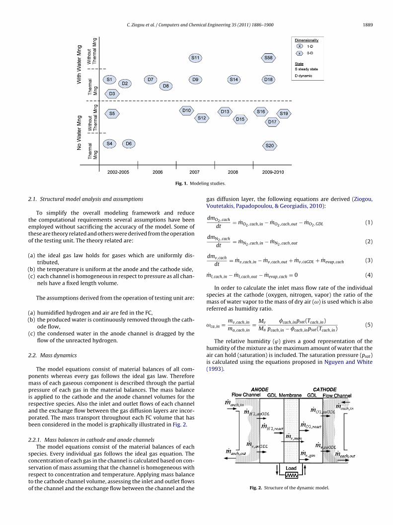
The aforementioned models describe the evolution of the semi-mpirical modeling approach. Although these models do notnclude many details of the system and they focus on specific oper-ting conditions, in contrast with the analytical and mechanisticFD models, they are very useful for application to real systems andontrol studies. A significant modeling effort has been done recentlyiming to achieve the proper tradeoff between the usability and theccuracy of the semi-empirical based models. A summary of keyontributions from the open literature is presented in Table 1. Thenumeration is based on the year of publication. For each work aummary is presented along with the dimensionality and the state.

Fig. 1 illustrates the dimensionality and the system state, alongith the existence of temperature and water management subsys-

ems.The presented models can be steady state or dynamic and they

tudy the response of the system to changes and its performancender various conditions. Each work has a specific purpose orientedowards fast development and considers only the required amountf detail needed for the scope of the project involved. It is impor-ant to note that these models are either one dimensional or lumpedarametric models. When the dimensionality is ignored, usually theemperature variation and the water handling are also ignored andise versa. The former focuses on simulating the fuel cell polar-zation curve while the latter generally pays more attention tohermodynamic aspects. These models are used in practical appli-ations and it has been recognized that although a large numberf theoretical models have been developed recently, an analogousumber of semi-empirical models has been developed too.

Compared to all these models, the model presented in this works developed for the purpose of on-line control in a power gen-ration unit. As such, it needs to have reduced execution timesnd enough accuracy for control. It is important to include detailsegarding the thermal behavior of the system as the regulation ofhe flow and the temperature are considered. Thus an approach thatombines both empirical and mechanistic equations is employed.he proposed model has the potential to couple both the theoreticalalidity and the inherent simplicity of the empirical application.

. Dynamic model of the PEM FC

The proposed model relies on mass and energy conserva-ion equations combined with equations having experimentally

defined parametric coefficients thus resulting in a semi-empiricaldynamic model. To model mass transport phenomena a five volumeapproach was adopted. The model accounts for mass dynamics inthe gas flow channels, the gas diffusion layers (GDL) and the mem-brane. The equation of the voltage as a function of the current andthe relationship between the current drawn from the fuel cell andthe consumption of the reactants describe the operation of the FC.Finally in this scheme the energy balance equation of the fuel cellwas also integrated.

C. Ziogou et al. / Computers and Chemical Engineering 35 (2011) 1886– 1900 1889

delin

2

teto

(

((

((

(

2

pmpirapb

2

scsrto

air can hold (saturation) is included. The saturation pressure (psat)is calculated using the equations proposed in Nguyen and White(1993).

Fig. 1. Mo

.1. Structural model analysis and assumptions

To simplify the overall modeling framework and reducehe computational requirements several assumptions have beenmployed without sacrificing the accuracy of the model. Some ofhese are theory related and others were derived from the operationf the testing unit. The theory related are:

a) the ideal gas law holds for gases which are uniformly dis-tributed,

b) the temperature is uniform at the anode and the cathode side,c) each channel is homogeneous in respect to pressure as all chan-

nels have a fixed length volume.

The assumptions derived from the operation of testing unit are:

a) humidified hydrogen and air are fed in the FC,b) the produced water is continuously removed through the cath-

ode flow,c) the condensed water in the anode channel is dragged by the

flow of the unreacted hydrogen.

.2. Mass dynamics

The model equations consist of material balances of all com-onents whereas every gas follows the ideal gas law. Thereforeass of each gaseous component is described through the partial

ressure of each gas in the material balances. The mass balances applied to the cathode and the anode channel volumes for theespective species. Also the inlet and outlet flows of each channelnd the exchange flow between the gas diffusion layers are incor-orated. The mass transport throughout each FC volume that haseen considered in the model is graphically illustrated in Fig. 2.

.2.1. Mass balances in cathode and anode channelsThe model equations consist of the material balances of each

pecies. Every individual gas follows the ideal gas equation. Theoncentration of each gas in the channel is calculated based on con-

ervation of mass assuming that the channel is homogeneous withespect to concentration and temperature. Applying mass balanceo the cathode channel volume, assessing the inlet and outlet flowsf the channel and the exchange flow between the channel and the

g studies.

gas diffusion layer, the following equations are derived (Ziogou,Voutetakis, Papadopoulou, & Georgiadis, 2010):

dmO2,cach

dt= mO2,cach,in − mO2,cach,out − mO2,GDL (1)

dmN2,cach

dt= mN2,cach,in − mN2,cach,out (2)

dmv,cach

dt= mv,cach,in − mv,cach,out + mv,caGDL + mevap,cach (3)

ml,cach,in − ml,cach,out − mevap,cach = 0 (4)

In order to calculate the inlet mass flow rate of the individualspecies at the cathode (oxygen, nitrogen, vapor) the ratio of themass of water vapor to the mass of dry air (ω) is used which is alsoreferred as humidity ratio.

ωca,in = mv,cach,in

ma,cach,in= Mv

Ma

�cach,inpsat(Tcach,in)pcach,in − �cach,inpsat(Tcach,in)

(5)

The relative humidity (ϕ) gives a good representation of thehumidity of the mixture as the maximum amount of water that the

Fig. 2. Structure of the dynamic model.

1 mical Engineering 35 (2011) 1886– 1900

e

m

m

m

c

m

a

x

x

mm

M

todttddod

m

m

t

m

s

m

um

p

p

ap

Table 2Flow parameter set.

Parameter Value

mfc 1.378 kgCpfc 772.57 J (kg K)−1

Afc 25 cm2

Vanch , Vcach 0.136 × 10−4 m3

ıanch , ıcach 1.25 mm

890 C. Ziogou et al. / Computers and Che

The mass flow rate of dry air (ma,cach,in) and vapor (mv,cach,in)ntering the cathode is

˙ cach,in = ma,cach,in + mv,cach,in (6)

˙ a,cach,in = 11 + ωca,in

mcach,in (7)

˙ v,cach,in = ωca,in

1 + ωca,inmcach,in (8)

The mass flow rates of the oxygen and nitrogen to the cathodehannel are calculated as follows:

˙ i,cach,in = xima,cach,in = xi1

1 + ωca,inmcach,in, i = [O2, N2] (9)

The mass fraction of oxygen (xO2 ) and nitrogen (xN2 ) in the dryir are defined as:

O2 = yO2 MO2 M−1˛ (10)

N2 = (1 − yO2 )MN2 M−1˛ (11)

The molar mass of dry air (M˛) is expressed by the sum of theass fraction of oxygen and nitrogen and the respective molarasses:

˛ = yO2 MO2 + (1 − yO2 )MN2 (12)

The above Eqs. (1)–(12) describe the dependence of masses fromhe inlet mass flows in the channel and the dynamics in the cath-de’s GDL. The outlet mass flows are also required to conclude theescription of the dynamics evolving at the cathode. We assumedhat no liquid water enters the cathode or the anode channel. Alsohe membrane allows only the transport of water in vapor state,ue to its waterproof nature. Therefore the liquid water is pro-uced by the reaction inside the cathode and part of it is evaporatedr condensed inside the channel. The evaporation/condensationynamics inside the cathode is expressed by:

˙ evap,cach = (psat(Tfc) − pv,cach)VcachkcondMv

RTfc(13)

The overall mass balance of the water in liquid phase is:

˙ l,cach,out = ml,caGDL − mevap,ca (14)

The outlet mass flow rate of the oxygen, nitrogen and vapor inhe cathode channel can be determined by:

˙ k,cach,out = mk,cach

ma,cach + mv,cachmcach,out, k = [O2, N2, v] (15)

At the cathode the condensed liquid water is dragged by the air,o the outlet flow is:

˙ cach,out = Kcach,out(pcach − pout) (16)

The partial pressures of the gases in the channel are calculatedsing the ideal gas law and the overall cathode pressure is deter-ined by the summation of the partial pressure of each species:

k,cach = RTfc

VcachMkmk,cach, k=[O2,N2,v] (17)

cach = pO2,cach + pN2,cach + pv,cach (18)

The equations that describe the anode part of the fuel cell arenalogous to the ones describing the cathode part. The values of allarameters used for channel dynamics are summarized in Table 2.

Kanch,out 0.001 kg/(bar s)Kcach,out 0.001 kg/(bar s)kcond 100 s−1

2.2.2. Gas diffusion layer (GDL) dynamicsEach gas diffusion layer is considered as a volume with homo-

geneous properties. A mixture of hydrogen and water vapor flowsthrough the anode GDL, while a mixture of oxygen, nitrogen, andwater vapor flows through the cathode GDL. The above gases mustdiffuse throughout the GDL to reach the membrane. Nitrogen dif-fusion is neglected since it is an inert gas. The oxygen and hydrogenmass flow rates between the GDL and the cathode and the anodechannel respectively are described by:

mk,GDL = AfcMkNk,GDL, k = [O2, H2] (19)

The molar flux of the vapor that is generated via the elec-trochemical reaction and the molar fluxes of the reactants arecalculated from the electric current and the stoichiometry of thereaction as follows:

Nv,gen = I

2FAfc(20)

NO2,GDL = I

4FAfc(21)

NH2,GDL = I

2FAfc(22)

The water vapor mass flow rate depends on the membraneactive area, the vapor molar mass and the vapor diffusion molarflux flow between GDL and anode and cathode:

mv,kGDL = AfcMH2ONv,k, k = [an, ca] (23)

where Nv,k is the molar flow rate per unit area (flux) of the vapordiffusion which is calculated by the effective diffusivity (Deff) thethickness of the diffusion channels (ıGDL) and the concentrationgradients (cv,anGDL,cv,caGDL):

Nv,k = −Deff,H2O(cv,kch − cv,kGDL)

ıGDL, k = [an, ca] (24)

As the oxygen is assumed to be in the same pressure with thechannel, diffusion will be imposed by the electrochemical reaction.The effective diffusion coefficient that will be used for the calcula-tion of the pressure is a function of the porosity (εpor) of the layeras described in Nam and Kaviany (2003):

Deff = Dref εpor

(εpor − εp

1 − εp

)da

(25)

where εp is a percolation threshold which for porous media iscomposed of two-dimensional, long and overlapping, random fiberlayers, εp is equal to 0.11 and da is an empirical constant which is0.785 for cross-plane diffusion (Dutta et al., 2001).

The partial pressure of water vapor in each GDL is calculatedthrough the respective mass balance equation:

dp(

N + N − N)

v,caGDL

dt= RTfc

v,gen v,mem v,ca

ıGDL(26)

dpv,anGDL

dt= RTfc

(Nv,an − Nv,mem

ıGDL

)(27)

mical Engineering 35 (2011) 1886– 1900 1891

o

p

p

2

rbwwfev

m

pitp

N

N

witc(

N

csa

c

v

�

tr

�

fi

n

b

D

Table 3Parameter set.

Parameter Value

Mmem,dry 1.1 kg mol−1

�mem,dry 1.98 × 103 kg m−3

−5

)

C. Ziogou et al. / Computers and Che

Since a uniform diffusion is assumed, the partial pressures ofxygen and hydrogen inside the respective GDL are expressed by:

O2,GDL = pO2,cach − RTfcıGDL

Deff,O2

NO2,GDL (28)

H2,GDL = pH2,anch − RTfcıGDL

Deff,H2

NH2,GDL (29)

.2.3. Membrane modelThe membrane hydration model calculates the water mass flow

ate that crosses the membrane and the water content in the mem-rane. Given that the membrane only allows the transport of vapourater, the following equations are only considering gaseous water,hich is also assumed to be uniformly distributed over the sur-

ace area of the membrane. A set of semi-empirical equations aremployed from Dutta et al. (2001). The overall mass flow rate ofapour that crosses the membrane is given by:

˙ v,memb = MH2OAfcNv,mem (30)

The flow of vapour water through membrane is affected by twohenomena, the electro-osmotic drag (Nv,osm), caused by hydrogen

on drag, and the back diffusion (Nv,diff), caused by water concen-ration gradient between the cathode and the anode. These twohenomena are mathematically expressed by:

v,osm = ndI

AfcF(31)

v,diff = awDwcv,cach − cv,anch

ımem(32)

here nd is the drag coefficient, Dw is the diffusion coefficient, ımem

s the membrane thickness and cv,anch, cv,cach are the water concen-ration in anode and cathode channel respectively. Based on theombination of those phenomena the net overall vapor molar flowNv,mem) across the membrane is expressed by:

v,mem = Nv,osm − Nv,diff (33)

The vapor concentration at anode and cathode surfaces (cv,anch,v,cach) of the membrane is a function of the water content at theseurfaces and it is calculated by the membrane dry density �mem,drynd the membrane dry equivalent weight Mmem,dry:

v,k = �mem,dry

Mmem,dry�k, k = [anch, cach] (34)

To calculate the water content at the membrane surfaces theapor activity inside each GDL is (Springer et al., 1991):

kch = 0.043 + 17.81˛k − 39.85˛2k + 36˛3

k, k = [an, ca] (35)

The vapor activity (˛k) is the ratio of the water vapor pressureo the saturation pressure which in case of gas it is equivalent toelative humidity (�k) of each GDL channel.

kGDL = pv,kGDL

psat(Tfc), k = [an, ca] (36)

The relationship between the water content at the anode sur-ace of the membrane and the electro-osmotic drag coefficient nds given by Dutta et al. (2001):

d = 0.0029�2anch + 0.05�anch − 3.4 × 10−19 (37)

The water diffusion coefficient (Dw) is expressed by the mem-rane water content at the anode surface:

w = D�anchexp

(2416

(1

303− 1

Tst

))(38)

ımem 8.89 × 10 mıGDL 1.9 × 10−5 mεpor 78%

where D�anchis modified based on the relative humidity level that

affects the water content at the anode surface (�anch):

D�anch=

⎧⎪⎨⎪⎩

10−10 �anch < 210−10(1 + 2(�anch − 2)) 2 ≤ �anch ≤ 310−10(3 − 1.67(�anch − 3)) 3 < �anch < 4.51.25 × 10−10 �anch ≥ 4.5

(39)

The physical parameters in the membrane model and the GDLdynamics are taken from the fuel cell specifications used on theactual unit. These parameters are summarized in Table 3.

2.3. Energy balance

A dynamic thermal model describes the dynamic behavior of thefuel cell temperature based on the overall energy balance equationof the fuel cell. The amount of energy which is not converted toelectrical power is expressed by a set of various energy terms, thatare associated with the fuel cell operation:

mfcCpfcdTfc

dt= Han + Hca + Hchem + QR − Qrad − Qconv − Pelec(40

The above equation takes into account the enthalpy flow rates asso-ciated with input and output streams at the anode and the cathode,the rate of energy produced by the chemical reaction, the rate ofenergy which is released to the environment through radiation, therate of heat transferred to the cooling system and finally the electricpower. The changes of the anode and cathode energy flow rates aregiven by the changes of enthalpy as follows:

Han = HH2 + HH2O,an (41)

Hca = HAir + HH2O,ca (42)

Only a part of the oxygen and hydrogen fed in the inlet chan-nels participate in the reaction. Therefore the remaining amountof energy pass through the system to the outlet. For each gas theenthalpy change is calculated as follows:

HH2 = mH2,anch,inhH2,an,in − mH2,anch,outhH2 (43)

HAir = (mO2,cach,inhO2,ca,in + mN2,cach,inhN2,ca,in)

− (mO2,cach,outhO2,ca + mN2,cach,outhN2,ca) (44)

HH2O,k = mv,kch,inhH2O,v,k,in

− (mv,kch,outHH2O,v + ml,kch,outhH2O,l), k = [an, ca]

(45)

It is assumed that the required energy for the change of waterphase is negligible therefore it is not incorporated in the aboveequations. In order to calculate the enthalpy differences at theanode and the cathode, the changes of mass specific enthalpies

with respect to a reference state of the participated gases are used,assuming constant specific heat.

hi,an,in = Cpi(Tan,in − Tref ), i = [H2, H2O, v] (46)

1 mical Engineering 35 (2011) 1886– 1900

w

ietc

ww

t

Q

wSf

gtipemc

Q

i

Q

w

ar

Q

h

wihd

b

Q

wus

2

orci

Table 4Thermal model parameters.

Parameter Value

Atot 355.27 × 10−4 m2

Acl 311.84 × 10−4 m2

hamb 1.73 × 10−3 W m−2 K−1

Kc1l 1.24Kcl2 1.38

892 C. Ziogou et al. / Computers and Che

hi,ca,in = Cpi(Tca,in − Tref ), i = [O2, N2, H2O, v] (47)

hi = Cpi(Tfc − Tref ), i = [H2, O2, N2, H2O, l, H2O, v] (48)

here Tref is the reference temperature.The reaction that converts the chemical energy into electric-

ty and forms liquid water is always exothermic and the producednthalpy is calculated as the difference between the enthalpy ofhe produced water and that of the reactants at the anode and theathode GDL.

Hchem = mH2,GDLhH2,an,in + mO2,GDLhO2,ca,in

− mH2O,gen

(Hr(Tref )

MH2O+ hH2O,v

)(49)

here H◦r is the mass specific enthalpy of formation of liquid

ater.A part of the produced heat is released to the environment

hrough radiation:

˙rad = εem� Atot(T4

fc − T4ref ) (50)

here εem is the emissivity of the fuel cell body, the � is thetefan–Boltzmann constant and Atot denotes the overall outer sur-ace of the fuel cell.

As stated earlier due to the reaction an excess amount of heat isenerated during the operation of the fuel cell since only a part ofhe produced enthalpy is converted to electrical energy and the rests converted to thermal energy, resulting in an increase of the tem-erature. Also as the fuel cell has a different temperature than itsnvironment, heat is lost through convection (Qconv) to its environ-ent. The amount of heat which is transferred to the surroundings

onsists of a natural convection term and a forced convection term.

˙ conv = Qamb + Qcl (51)

The heat loss to the environment caused by natural convections expressed by:

˙amb = hambAtot(Tfc − Tref ) (52)

here hamb is the natural convection heat transfer coefficient.A cooling system is used for the removal of the excess heat

nd to maintain the desired fuel cell temperature. The heat energyemoved by the cooling system is expressed by:

˙cl = hforcAcl(Tfc − Tcl) (53)

forc = Kcl1PKcl2cl (54)

here hforc is the forced convective heat transfer coefficient and Acls the effective surface for the cooling system. The forced convectioneat transfer coefficient is calculated based on two experimentallyefined parameters (Kcl1,Kcl2) and the power (Pcl) of the fans.

The heat supply for the initial heat up of the fuel cell is expressedy:

˙ R = PRxR (55)

here PR is the power of the heater and xR is the fraction of powersed for heating. The parameters used in the energy balance areummarized in Table 4.

.4. Electrochemical equations

Typical characteristics of FC are normally expressed in the form

f a polarization curve, which is a plot of cell voltage versus cell cur-ent density. To determine the voltage–current relationship of theell, the cell voltage has to be defined as the difference between andeal Nernst voltage and a number of voltage losses as it is described

PR 55.8 WPcl 25 W

in the current section. The main losses are categorized as activa-tion, ohmic and concentration losses. The equation that takes intoconsideration the above losses expresses the actual cell voltage:

Vcell = Enernst − Vact − Vohm − Vconc (56)

The above equation is able to predict the voltage output of PEMfuel cells of various configurations. Depending on the amount ofcurrent drawn the fuel cell generates the output voltage. The elec-tric power produced by the system equals the product of the stackvoltage Vcell and the current drawn I:

P = I · Vcell (57)

The Nernst voltage or open circuit voltage (OCV) falls as thecurrent supplied by the stack increases. The reversible thermody-namic potential is calculated using the Nerst equation and can beexpressed:

Enerst = E0 + RT

2Fln(pH2 p1/2

O2p−1

H2O) (58)

The activation losses are caused by the slowness of the reactionstaking place on the surface of the electrodes. A portion of the voltagegenerated is lost because of the chemical reaction that transfersthe electrons to or from the electrodes. The activation losses aredescribed by the Tafel equation (Mann et al., 2000), which can becalculated as:

Vact = �1 + �2T + �3Tst ln(I) + �4Tst ln(cO2) (59)

This description for the activation overvoltage takes intoaccount the concentration of oxygen at the catalyst layer and vari-ous experimentally defined parametric coefficients.

At a later stage of the fuel cell operation, as current densityrises, ohmic losses (Vohm) prevail. They are derived from the mem-brane resistance to the flow of electrons through the material ofthe electrodes and the various interconnections, as well as by theresistance to the flow of protons through the electrolyte (Pathapatiet al., 2004):

Vohm = (�5 + �6T + �7I)I (60)

Finally the mass transport or concentration losses result fromthe change in concentration of the reactants at the surface of theelectrodes as the fuel is used. To calculate the diffusion losses asemi-empirical equation by (Kim et al., 1995) was used:

Vconc = �8 exp(�9I) (61)

The empirical parameters are related to the conductivity of theelectrolyte (�8) and to the porosity of the gas diffusion layer (�9). Inthe above equations �k (k = 1..9) represent experimentally definedparametric coefficients the value which can vary from stack to

stack. The values of these parameters are presented in Table 5.Some of these parameters are defined by the estimation procedureas described in the subsequent Section 4.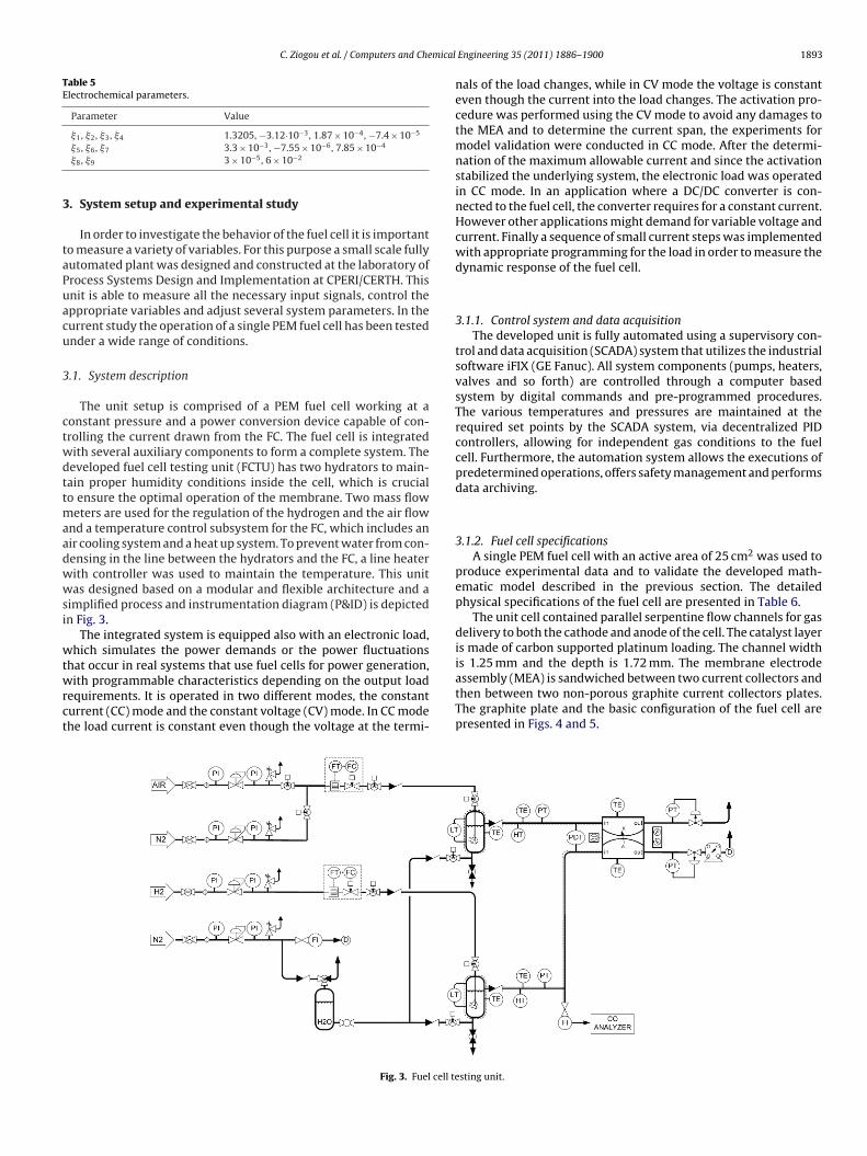

C. Ziogou et al. / Computers and Chemical

Table 5Electrochemical parameters.

Parameter Value

�1, �2, �3, �4 1.3205, −3.12·10−3, 1.87 × 10−4, −7.4 × 10−5

3

taPuacu

3

ctwdttmaadwwsi

wtwrct

�5, �6, �7 3.3 × 10−3, −7.55 × 10−6, 7.85 × 10−4

�8, �9 3 × 10−5, 6 × 10−2

. System setup and experimental study

In order to investigate the behavior of the fuel cell it is importanto measure a variety of variables. For this purpose a small scale fullyutomated plant was designed and constructed at the laboratory ofrocess Systems Design and Implementation at CPERI/CERTH. Thisnit is able to measure all the necessary input signals, control theppropriate variables and adjust several system parameters. In theurrent study the operation of a single PEM fuel cell has been testednder a wide range of conditions.

.1. System description

The unit setup is comprised of a PEM fuel cell working at aonstant pressure and a power conversion device capable of con-rolling the current drawn from the FC. The fuel cell is integratedith several auxiliary components to form a complete system. Theeveloped fuel cell testing unit (FCTU) has two hydrators to main-ain proper humidity conditions inside the cell, which is crucialo ensure the optimal operation of the membrane. Two mass flow

eters are used for the regulation of the hydrogen and the air flownd a temperature control subsystem for the FC, which includes anir cooling system and a heat up system. To prevent water from con-ensing in the line between the hydrators and the FC, a line heaterith controller was used to maintain the temperature. This unitas designed based on a modular and flexible architecture and a

implified process and instrumentation diagram (P&ID) is depictedn Fig. 3.

The integrated system is equipped also with an electronic load,hich simulates the power demands or the power fluctuations

hat occur in real systems that use fuel cells for power generation,

ith programmable characteristics depending on the output load

equirements. It is operated in two different modes, the constanturrent (CC) mode and the constant voltage (CV) mode. In CC modehe load current is constant even though the voltage at the termi-

Fig. 3. Fuel cell te

Engineering 35 (2011) 1886– 1900 1893

nals of the load changes, while in CV mode the voltage is constanteven though the current into the load changes. The activation pro-cedure was performed using the CV mode to avoid any damages tothe MEA and to determine the current span, the experiments formodel validation were conducted in CC mode. After the determi-nation of the maximum allowable current and since the activationstabilized the underlying system, the electronic load was operatedin CC mode. In an application where a DC/DC converter is con-nected to the fuel cell, the converter requires for a constant current.However other applications might demand for variable voltage andcurrent. Finally a sequence of small current steps was implementedwith appropriate programming for the load in order to measure thedynamic response of the fuel cell.

3.1.1. Control system and data acquisitionThe developed unit is fully automated using a supervisory con-

trol and data acquisition (SCADA) system that utilizes the industrialsoftware iFIX (GE Fanuc). All system components (pumps, heaters,valves and so forth) are controlled through a computer basedsystem by digital commands and pre-programmed procedures.The various temperatures and pressures are maintained at therequired set points by the SCADA system, via decentralized PIDcontrollers, allowing for independent gas conditions to the fuelcell. Furthermore, the automation system allows the executions ofpredetermined operations, offers safety management and performsdata archiving.

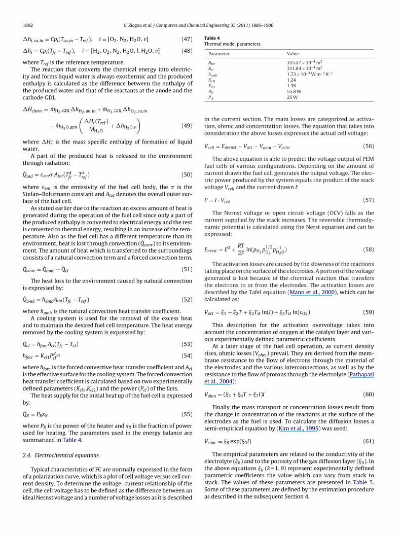
3.1.2. Fuel cell specificationsA single PEM fuel cell with an active area of 25 cm2 was used to

produce experimental data and to validate the developed math-ematic model described in the previous section. The detailedphysical specifications of the fuel cell are presented in Table 6.

The unit cell contained parallel serpentine flow channels for gasdelivery to both the cathode and anode of the cell. The catalyst layeris made of carbon supported platinum loading. The channel widthis 1.25 mm and the depth is 1.72 mm. The membrane electrode

assembly (MEA) is sandwiched between two current collectors andthen between two non-porous graphite current collectors plates.The graphite plate and the basic configuration of the fuel cell arepresented in Figs. 4 and 5.

sting unit.

1894 C. Ziogou et al. / Computers and Chemical Engineering 35 (2011) 1886– 1900

Table 6System physical parameters.

Description Value

Nominal cell voltage 0.6 ± 0.05 VNominal current density 400 ± 50 mA/cm2

Operating temperature 60–75 ◦CTotal mass 1.378 kgSpecific heat capacity 772.57 J (kg K)−1

Active area 25 cm2 (5 cm × 5 cm)Channel volume (anode, cathode) 0.136 × 10−4 m3

Membrane type Nafion 1135Backing layer catalyst loading 20 wt.% Pt/CGDL type Carbon paperBulk density 0.44 g cm−3

Heater resistance 0.867 k� (55.8 W)

3

esaMtbsiwiva

0.4

0.5

0.6

0.7

0.8

0.9

1

0

1

2

3

4

5

6

7

0 0.1 0.2 0.3 0.4 0.5 0.6 0.7 0.8

V (1st act A)V (1st act B)V (1st act C)V (1st act D)

P (1st act A)P (1st act B)P (1st act C)P (1st act D)

Volta

ge (V

) Pow

er (W)

Nominal Poin t

Fig. 4. Flow plate.

.2. Experimental study

Various experimental studies can be found in the literaturexploring the dynamic behavior of a PEM fuel cell system. Eachtudy focuses on a different aspect of the fuel ell operation suchs step changes in current with operating temperature (Kim andin, 2008), start-up behavior (Chen and Zhou, 2008), characteriza-

ion of the electrical behavior (Kunusch et al., 2010), individual cellehavior (Jang et al., 2008; Sun et al., 2009). In this study the steadytate and the dynamic behavior of the single PEM fuel cell system isnvestigated under various operating conditions. The single cell that

as tested during our study was not conditioned, therefore after

nitial stabilization, the membrane had to be activated. The acti-ation procedure was divided into two stages, the initial activationnd the full activation of the membrane. The distinguishing charac-

Fig. 5. Single PEM FC.

Current Density (A/cm^2)

Fig. 6. Initial activation stage (1.0. . .0.45 V).

teristic between these stages was the minimum allowable voltage.Afterwards the performance of the system was tested against var-ious conditions.

3.2.1. Activation procedureThe activation procedure consisted of reading the dynamic

response of the cell voltage after the occurrence of small changesin the current load. A series of small fixed length step changes incurrent load with a specific range were applied, which constitute acycle. A reference voltage point was set (Vref = 0.45 V) and used asan indicative point of comparison between each cycle in order tomeasure the evolution of the membrane activation. The nominalpoint of operation provided by the manufacturer was 0.40 A/cm2

at 0.6 V and it constitutes an indication the membrane is ready foruse. During the initial activation the voltage demand was regulatedthrough a ramp procedure and gradually decreased from 1.0 V to0.45 V and conversely with a step change of 100 mV every 10 s. OnFig. 8 the evolution of the current and power density are presented.

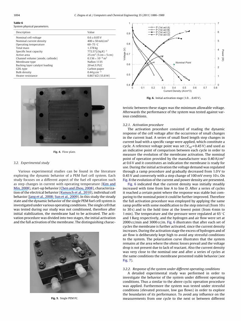
Fig. 6 indicated that the current density was initially steadilyincreased with time from line A to line D. After a series of cyclesit reached a certain point where the response was stable but com-paring to the nominal point it could be further improved. Thereforethe full activation procedure was employed by applying the sameramp profile with some modification to the step interval (from 10 sto 30 s) and to the hold time at the lowest point (from 4 min to1 min). The temperature and the pressure were regulated at 65 ◦Cand 1 Barg respectively, and the hydrogen and air flow were set at2000 cc/min and 3000 cc/m. Fig. 6 illustrates that after each set ofcycles the membrane is further activated, since the current densityincreases. During the activation stage the excess of hydrogen and ofair flow is deliberately kept high to avoid any stressful conditionsto the system. The polarization curve illustrates that the systemremains at the area where the ohmic losses prevail and the voltagedrop is not present due to lack of reactant. Also the current densitywas very close to the nominal one and after a series of cycles atthe same conditions the membrane presented stable behavior (seeFig. 7).

3.2.2. Response of the system under different operating conditionsA detailed experimental study was performed in order to

investigate the behavior of the system under different operatingconditions. Thus a similar to the above cyclic operation procedure

was applied. Furthermore the system was tested under stressfulconditions (elevated pressure, low gas flows) in order to explorethe boundaries of its performance. To avoid any influence on themeasurements from one cycle to the next or between different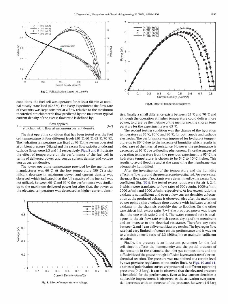

C. Ziogou et al. / Computers and Chemical Engineering 35 (2011) 1886– 1900 1895

0

0.2

0.4

0.6

0.8

1

0

1

2

3

4

5

6

7

0 0.2 0.4 0.6 0.8

V (2nd act A)V (2nd act B)V (2nd act C)V (2nd act D)

P (2nd act A)P (2nd act B)P (2nd act C)P (2nd act D)

Vol

tage

(V) P

ower (W

)

Nominal Point

cnotc

�

cTacttv

mnonut

0

1

2

3

4

5

6

7

0 0.1 0.2 0.3 0.4 0.5 0.6 0.7 0.8

P (TE: 50°C)P (TE: 60°C)P (TE: 65°C)P (TE: 70°C)

Pow

er (W

)

Current Density (A/cm^2)

Current Density (A/cm^2 )

Fig. 7. Full activation stage (1.0. . .0.0 V).

onditions, the fuel cell was operated for at least 60 min at nomi-al steady-state load (0.45 V). For every experiment the flow ratef reactants was kept constant at a flow relative to the maximumheoretical stoichiometric flow predicted by the maximum typicalurrent density of the excess flow ratio is defined by:

= flow appliedstoichiometric flow at maximum current density

(62)

The first operating condition that has been tested was the fuelell temperature at four different levels (50 ◦C, 60 ◦C, 65 ◦C, 70 ◦C).he hydration temperature was fixed at 70 ◦C, the system operatedt ambient pressure (0 Barg) and the excess flow ratio for anode andathode flows were 2.3 and 1.5 respectively. Figs. 8 and 9 illustratehe effect of temperature on the performance of the fuel cell inerms of delivered power and versus current density and voltageersus current density.

The lower operating temperature provided by the membraneanufacturer was 60 ◦C. At the low temperature (50 ◦C) a sig-

ificant decrease in maximum power and current density wasbserved, which indicated that the full capacity of the fuel cell was

ot utilized. Between 60 ◦C and 65 ◦C the performance was similarp to the maximum delivered power but after that, the power athe elevated temperature was decreased at higher current densi-

0

0.2

0.4

0.6

0.8

1

0 0.1 0.2 0.3 0.4 0.5 0.6 0.7 0.8

V (TE: 50 °C)V (TE: 60 °C)V (TE: 65 °C)V (TE: 70 °C)

Vol

tage

(V)

Current Density (A/cm^2)

Fig. 8. Effect of temperature to voltage.

Fig. 9. Effect of temperature to power.

ties. Finally a small difference exists between 65 ◦C and 70 ◦C andalthough the operation at higher temperature could deliver morepower, to preserve the lifetime of the membrane, the chosen tem-perature for the experiments was 65 ◦C.

The second testing condition was the change of the hydrationtemperature at 65 ◦C, 80 ◦C and 90 ◦C, for both anode and cathodeelectrodes. The performance was improved for hydrators temper-ature up to 80 ◦C due to the increase of humidity which results ina decrease of the internal resistance. However the performance isdecreased at 90 ◦C due to flooding phenomena. Since the suggestedoperating temperature from the previous experiment is 65 ◦C thehydrators temperature is chosen to be 5 ◦C to 10 ◦C higher. Thisresults to avoid flooding and at the same time the membrane wasadequately humidified.

After the investigation of the temperature and the humidityeffect the flow rate and the pressure are investigated. For every case,the mass flow rates of reactants were determined by the excess flowcoefficient (Eq. (62)). The tested excess ratios were for air 1, 2, 4,6 which were translated to flow rates of 500 cc/min, 1000 cc/min,2000 cc/min and 3000 cc/min respectively. At low excess ratio theoxidant is not sufficient and even at low current densities a fluctu-ation at the produced voltage is observed. Also after the maximumpower point a sharp voltage drop appears with indicates a lack ofoxidants in the channels probably due to flooding. On the othercase side at high excess ratio (� = 6) the produced power was lowerthan the one with ratio 2 and 4. The water removal rate is anal-ogous to the air flow rate which causes drying of the membraneand an increase to the electrical resistance. Therefore any ratiobetween 2 and 4 can deliver satisfactory results. The hydrogen flowrate had very limited influence on the performance and it was setto a stoichiometric ratio of 2.3 (500 cc/m) to maintain sufficientreaction.

Finally, the pressure is an important parameter for the fuelcell, since it affects the homogeneity and the partial pressure ofthe reactants in the channels, the inlet gas compositions and thediffusivities of the gases through diffusion layers and rate of electro-chemical reaction. The pressure was maintained at a certain levelby two pressure regulators at the outlet lines. At Figs. 10 and 11,a series of polarization curves are presented at different operating

pressures (0–2 Barg). It can be observed that the elevated pressureis beneficial for the performance. Even at low current densities anoticeable improvement is observed as the activation overpoten-tial decreases with an increase of the pressure. Between 1.5 Barg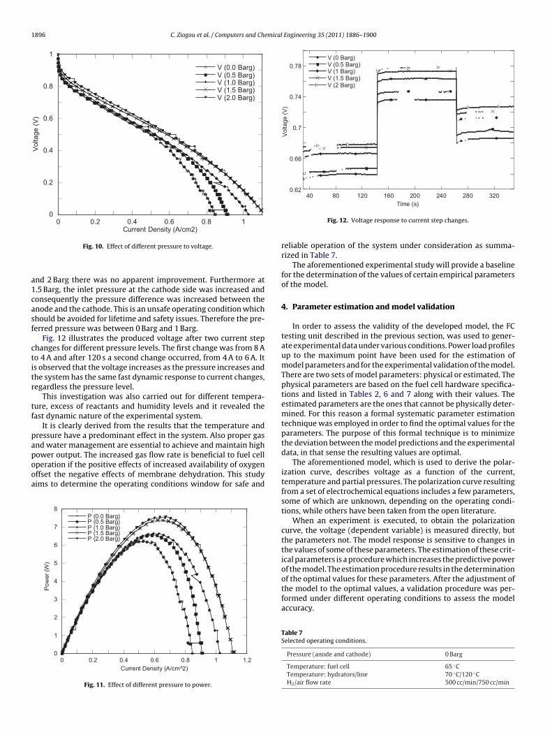

1896 C. Ziogou et al. / Computers and Chemical Engineering 35 (2011) 1886– 1900

0

0.2

0.4

0.6

0.8

1

0 0.2 0.4 0.6 0.8 1

V (0.0 Barg)V (0.5 Barg)V (1.0 Barg)V (1.5 Barg)V (2.0 Barg)

Vol

tage

(V)

Current Density (A/cm2)

a1casf

ctitr

tf

papooa

0.62

0.66

0.7

0.74

0.78

40 80 120 16 0 200 240 280 320

V (0 Barg )V (0.5 Bar g)V (1 Barg )V (1.5 Bar g)V (2 Barg )

Vol

tage

(V)

Time (s)

Fig. 10. Effect of different pressure to voltage.

nd 2 Barg there was no apparent improvement. Furthermore at.5 Barg, the inlet pressure at the cathode side was increased andonsequently the pressure difference was increased between thenode and the cathode. This is an unsafe operating condition whichhould be avoided for lifetime and safety issues. Therefore the pre-erred pressure was between 0 Barg and 1 Barg.

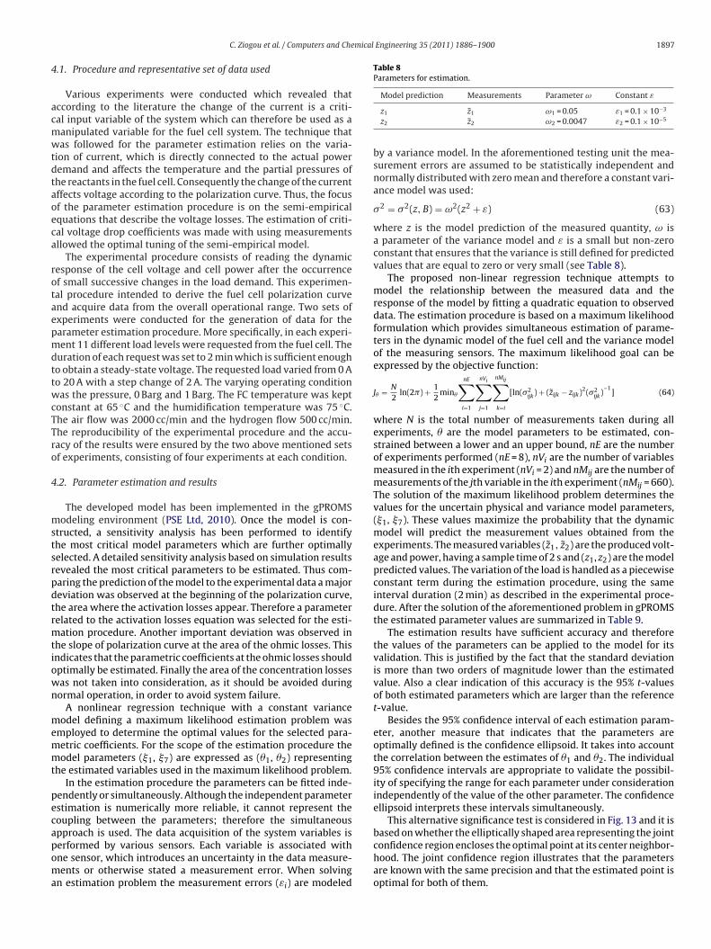
Fig. 12 illustrates the produced voltage after two current stephanges for different pressure levels. The first change was from 8 Ao 4 A and after 120 s a second change occurred, from 4 A to 6 A. Its observed that the voltage increases as the pressure increases andhe system has the same fast dynamic response to current changes,egardless the pressure level.

This investigation was also carried out for different tempera-ure, excess of reactants and humidity levels and it revealed theast dynamic nature of the experimental system.

It is clearly derived from the results that the temperature andressure have a predominant effect in the system. Also proper gasnd water management are essential to achieve and maintain highower output. The increased gas flow rate is beneficial to fuel cell

peration if the positive effects of increased availability of oxygenffset the negative effects of membrane dehydration. This studyims to determine the operating conditions window for safe and

0

1

2

3

4

5

6

7

8

0 0.2 0.4 0.6 0.8 1 1.2

P (0.0 Barg)P (0.5 Barg)P (1.0 Barg)P (1.5 Barg)P (2.0 Barg)

Pow

er (W

)

Current Density (A/cm^2)

Fig. 11. Effect of different pressure to power.

Fig. 12. Voltage response to current step changes.

reliable operation of the system under consideration as summa-rized in Table 7.

The aforementioned experimental study will provide a baselinefor the determination of the values of certain empirical parametersof the model.

4. Parameter estimation and model validation

In order to assess the validity of the developed model, the FCtesting unit described in the previous section, was used to gener-ate experimental data under various conditions. Power load profilesup to the maximum point have been used for the estimation ofmodel parameters and for the experimental validation of the model.There are two sets of model parameters: physical or estimated. Thephysical parameters are based on the fuel cell hardware specifica-tions and listed in Tables 2, 6 and 7 along with their values. Theestimated parameters are the ones that cannot be physically deter-mined. For this reason a formal systematic parameter estimationtechnique was employed in order to find the optimal values for theparameters. The purpose of this formal technique is to minimizethe deviation between the model predictions and the experimentaldata, in that sense the resulting values are optimal.

The aforementioned model, which is used to derive the polar-ization curve, describes voltage as a function of the current,temperature and partial pressures. The polarization curve resultingfrom a set of electrochemical equations includes a few parameters,some of which are unknown, depending on the operating condi-tions, while others have been taken from the open literature.

When an experiment is executed, to obtain the polarizationcurve, the voltage (dependent variable) is measured directly, butthe parameters not. The model response is sensitive to changes inthe values of some of these parameters. The estimation of these crit-ical parameters is a procedure which increases the predictive powerof the model. The estimation procedure results in the determinationof the optimal values for these parameters. After the adjustment of

the model to the optimal values, a validation procedure was per-formed under different operating conditions to assess the modelaccuracy.

Table 7Selected operating conditions.

Pressure (anode and cathode) 0 Barg

Temperature: fuel cell 65 ◦CTemperature: hydrators/line 70 ◦C/120 ◦CH2/air flow rate 500 cc/min/750 cc/min

mical Engineering 35 (2011) 1886– 1900 1897

4

acmwtdtaoeca

rotaepmdttwcTTro

4

mstsrpdtrmtiown

memmt

pecapoma

Table 8Parameters for estimation.

Model prediction Measurements Parameter ω Constant ε

C. Ziogou et al. / Computers and Che

.1. Procedure and representative set of data used

Various experiments were conducted which revealed thatccording to the literature the change of the current is a criti-al input variable of the system which can therefore be used as aanipulated variable for the fuel cell system. The technique thatas followed for the parameter estimation relies on the varia-

ion of current, which is directly connected to the actual poweremand and affects the temperature and the partial pressures ofhe reactants in the fuel cell. Consequently the change of the currentffects voltage according to the polarization curve. Thus, the focusf the parameter estimation procedure is on the semi-empiricalquations that describe the voltage losses. The estimation of criti-al voltage drop coefficients was made with using measurementsllowed the optimal tuning of the semi-empirical model.

The experimental procedure consists of reading the dynamicesponse of the cell voltage and cell power after the occurrencef small successive changes in the load demand. This experimen-al procedure intended to derive the fuel cell polarization curvend acquire data from the overall operational range. Two sets ofxperiments were conducted for the generation of data for thearameter estimation procedure. More specifically, in each experi-ent 11 different load levels were requested from the fuel cell. The

uration of each request was set to 2 min which is sufficient enougho obtain a steady-state voltage. The requested load varied from 0 Ao 20 A with a step change of 2 A. The varying operating conditionas the pressure, 0 Barg and 1 Barg. The FC temperature was kept

onstant at 65 ◦C and the humidification temperature was 75 ◦C.he air flow was 2000 cc/min and the hydrogen flow 500 cc/min.he reproducibility of the experimental procedure and the accu-acy of the results were ensured by the two above mentioned setsf experiments, consisting of four experiments at each condition.

.2. Parameter estimation and results

The developed model has been implemented in the gPROMSodeling environment (PSE Ltd, 2010). Once the model is con-

tructed, a sensitivity analysis has been performed to identifyhe most critical model parameters which are further optimallyelected. A detailed sensitivity analysis based on simulation resultsevealed the most critical parameters to be estimated. Thus com-aring the prediction of the model to the experimental data a majoreviation was observed at the beginning of the polarization curve,he area where the activation losses appear. Therefore a parameterelated to the activation losses equation was selected for the esti-ation procedure. Another important deviation was observed in

he slope of polarization curve at the area of the ohmic losses. Thisndicates that the parametric coefficients at the ohmic losses shouldptimally be estimated. Finally the area of the concentration lossesas not taken into consideration, as it should be avoided duringormal operation, in order to avoid system failure.

A nonlinear regression technique with a constant varianceodel defining a maximum likelihood estimation problem was

mployed to determine the optimal values for the selected para-etric coefficients. For the scope of the estimation procedure theodel parameters (�1, �7) are expressed as (�1, �2) representing

he estimated variables used in the maximum likelihood problem.In the estimation procedure the parameters can be fitted inde-

endently or simultaneously. Although the independent parameterstimation is numerically more reliable, it cannot represent theoupling between the parameters; therefore the simultaneouspproach is used. The data acquisition of the system variables is

erformed by various sensors. Each variable is associated withne sensor, which introduces an uncertainty in the data measure-ents or otherwise stated a measurement error. When solving

n estimation problem the measurement errors (εi) are modeled

z1 z1 ω1 = 0.05 ε1 = 0.1 × 10−3

z2 z2 ω2 = 0.0047 ε2 = 0.1 × 10−5

by a variance model. In the aforementioned testing unit the mea-surement errors are assumed to be statistically independent andnormally distributed with zero mean and therefore a constant vari-ance model was used:

�2 = �2(z, B) = ω2(z2 + ε) (63)

where z is the model prediction of the measured quantity, ω isa parameter of the variance model and ε is a small but non-zeroconstant that ensures that the variance is still defined for predictedvalues that are equal to zero or very small (see Table 8).

The proposed non-linear regression technique attempts tomodel the relationship between the measured data and theresponse of the model by fitting a quadratic equation to observeddata. The estimation procedure is based on a maximum likelihoodformulation which provides simultaneous estimation of parame-ters in the dynamic model of the fuel cell and the variance modelof the measuring sensors. The maximum likelihood goal can beexpressed by the objective function:

J� = N

2ln(2 ) + 1

2min�

nE∑i=1

nVi∑j=1

nMij∑k=i

[ln(�2ijk

) + (zijk − zijk)2(�2ijk

)−1

] (64)

where N is the total number of measurements taken during allexperiments, � are the model parameters to be estimated, con-strained between a lower and an upper bound, nE are the numberof experiments performed (nE = 8), nVi are the number of variablesmeasured in the ith experiment (nVi = 2) and nMij are the number ofmeasurements of the jth variable in the ith experiment (nMij = 660).The solution of the maximum likelihood problem determines thevalues for the uncertain physical and variance model parameters,(�1, �7). These values maximize the probability that the dynamicmodel will predict the measurement values obtained from theexperiments. The measured variables (z1, z2) are the produced volt-age and power, having a sample time of 2 s and (z1, z2) are the modelpredicted values. The variation of the load is handled as a piecewiseconstant term during the estimation procedure, using the sameinterval duration (2 min) as described in the experimental proce-dure. After the solution of the aforementioned problem in gPROMSthe estimated parameter values are summarized in Table 9.

The estimation results have sufficient accuracy and thereforethe values of the parameters can be applied to the model for itsvalidation. This is justified by the fact that the standard deviationis more than two orders of magnitude lower than the estimatedvalue. Also a clear indication of this accuracy is the 95% t-valuesof both estimated parameters which are larger than the referencet-value.

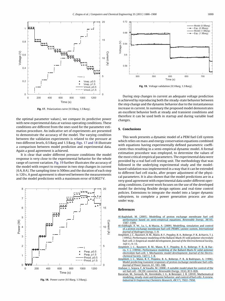
Besides the 95% confidence interval of each estimation param-eter, another measure that indicates that the parameters areoptimally defined is the confidence ellipsoid. It takes into accountthe correlation between the estimates of �1 and �2. The individual95% confidence intervals are appropriate to validate the possibil-ity of specifying the range for each parameter under considerationindependently of the value of the other parameter. The confidenceellipsoid interprets these intervals simultaneously.

This alternative significance test is considered in Fig. 13 and it isbased on whether the elliptically shaped area representing the joint

confidence region encloses the optimal point at its center neighbor-hood. The joint confidence region illustrates that the parametersare known with the same precision and that the estimated point isoptimal for both of them.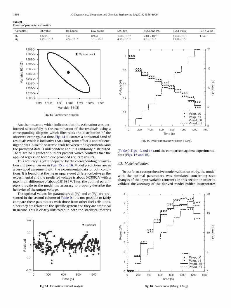

1898 C. Ziogou et al. / Computers and Chemical Engineering 35 (2011) 1886– 1900

Table 9Results of parameter estimation.

Variables Est. value Up bound Low bound Std. dev. 95% Conf. Int. 95% t-value Ref. t-value

�1 1.3205 1.4 0.954 1.04 × 10−3 2.04 × 10−3 6.464 × 102 1.645�2 7.85 × 10−4 4.3 × 10−3 1.1 × 10−6 4.12 × 10−6 8.1 × 10−6 0.969 × 102

7.80 E-04

7.81 E-04

7.82 E-04

7.83 E-04

7.84 E-04

7.85 E-04

7.86 E-04

7.87 E-04

7.88 E-04

7.89 E-04

7.90 E-04

1.319 1.319 5 1.32 1.320 5 1.321 1.321 5 1.322

Var

iabl

e θ2

(ξ7)

Optimal point

fcoritTa

tatemeb

scsi

0

0.2

0.4

0.6

0.8

1

0

5

10

15

20

0 200 400 600 800 1000 1200 1400

Vexp, p0Vexp, p1Vmod, p0Vmod, p1

I

Vol

tage

(V) C

urrent (A)

To perform a comprehensive model validation study, the modelwith the optimal parameters was simulated concerning stepchanges of the input variable (current). In this section in order tovalidate the accuracy of the derived model (which incorporates

8 20

Variable θ1 (ξ1)

Fig. 13. Confidence ellipsoid.

Another measure which indicates that the estimation was per-ormed successfully is the examination of the residuals using aorresponding diagram which illustrates the distribution of thebserved error against time. Fig. 14 illustrates a horizontal band ofesiduals which is indicative that a long-term effect is not influenc-ng the data. Also the observed error between the experimental andhe predicted data is independent and it is randomly distributed.here are no significant outliers present which confirms that thepplied regression technique provided accurate results.

This accuracy is better depicted by the corresponding polariza-ion and power curves in Figs. 15 and 16. Model predictions are in

very good agreement with the experimental data for both condi-ions. It is found that the mean square-root difference between thexperimental and the predicted voltage is about 0.03892 V with aaximum difference of about 0.01987 V. Thus, the optimal param-

ters provide to the model the accuracy to properly describe theehavior of the output voltage.

The optimal values for parameters �1(�1) and �7(�2) are pre-

ented in the second column of Table 9. It is not possible to fairlyompare these parameters with those from other fuel cells units,ince they are related to the specific system and they are empiricaln nature. This is clearly illustrated in both the statistical metrics

-0.02

-0.01

0

0.01

0.02

0 30 0 60 0 90 0 120 0Time (s)

Res

idua

l

Residual

Fig. 14. Estimation residual analysis.

Time (s)

Fig. 15. Polarization curve (0 Barg, 1 Barg).

(Table 9, Figs. 13 and 14) and the comparison against experimentaldata (Figs. 15 and 16).

4.3. Model validation

0

1

2

3

4

5

6

7

0

5

10

15

0 200 400 600 800 1000 1200 1400

Pexp, p0Pexp, p1Pmod, p0Pmod, p1

I

Pow

er (W

) Current (A

)

Time (s)

Fig. 16. Power curve (0 Barg, 1 Barg).

C. Ziogou et al. / Computers and Chemical Engineering 35 (2011) 1886– 1900 1899

0

0.2

0.4

0.6

0.8

1

0

5

10

15

20

0 200 400 600 800 1000 1200

Vexp, p0.5Vexp, p1.5Vmod, p0.5Vmod, p1.5

I

Vol

tage

(V) C

urrent (A)

Time (s)

twcmtbtaA

rrt(ia

0.56

0.6

0.64

0.68

0.72

500 550 600 650 700

Model (0.5 Barg)Exp. (0.5Barg)Model (1.5 Barg)Exp. (1.5Barg)

Volta

ge (V

)

Fig. 17. Polarization curve (0.5 Barg, 1.5 Barg).

he optimal parameter values), we compare its predictive powerith new experimental data at various operating conditions. These

onditions are different from the ones used for the parameter esti-ation procedure. An indicative set of experiments are presented

o demonstrate the accuracy of the model. The varying conditionetween the validation experiments is related to the pressure atwo different levels, 0.5 Barg and 1.5 Barg. Figs. 17 and 18 illustrate

comparison between model prediction and experimental data.gain a good agreement is achieved.

It is clear that under different pressure conditions the modelesponse is very close to the experimental behavior for the wholeange of current variation. Fig. 19 further illustrates the accuracy ofhe model with respect to response in two step changes in current

6 A, 8 A). The sampling time is 500ms and the duration of each steps 120 s. A good agreement is observed between the measurementsnd the model predictions with a maximum error of 0.0027 V.

0

1

2

3

4

5

6

7

8

0

5

10

15

20

0 200 400 600 800 1000 1200

Pexp, p0.5Pexp, p1.5Pmod , p0.5Pmod , p1.5

I

Pow

er (W

) Current (A

)

Time (s)

Fig. 18. Power curve (0.5 Barg, 1.5 Barg).

Time (s)

Fig. 19. Voltage validation (0.5 Barg, 1.5 Barg).

During step changes in current an adequate voltage predictionis achieved by reproducing both the steady-state behavior betweenthe step change and the dynamic behavior due to the instantaneousincrease in current. In summary the proposed model demonstratesan excellent behavior both at steady and transient conditions andtherefore it can be used both in startup and during variable loadchanges.

5. Conclusions

This work presents a dynamic model of a PEM fuel Cell systemwhich relies on mass and energy conservation equations combinedwith equations having experimentally defined parametric coeffi-cients thus resulting in a semi-empirical dynamic model. A formalestimation procedure was employed, to determine the values ofthe most critical empirical parameters. The experimental data wereprovided by a real fuel cell testing unit. The methodology that wasfollowed in the underlying experimental study and the model-based validation was implemented in a way that it can be extendedto different fuel cell stacks, after proper adjustment of the physi-cal parameters. It is also shown that the model predictions are in avery good agreement with experimental data under different oper-ating conditions. Current work focuses on the use of the developedmodel for deriving flexible design options and real-time controlpolicies. Extensions to integrate the model into a larger dynamicsubsystem, to complete a power generation process are alsounder way.

References

Al-Baghdadi, M. (2005). Modelling of proton exchange membrane fuel cellperformance based on semi-empirical equations. Renewable Energy, 30(10),1587–1599.

Al-Dabbagh, A. W., Lu, L., & Mazza, A. (2009). Modelling, simulation and controlof a proton exchange membrane fuel cell (PEMFC) power system. InternationalJournal of Hydrogen Energy, 1–9.

Amphlett, J. C., Baumert, R. M., Mann, R. F., Peppley, B. A., Roberge, P. R., & Harris, T. J.(1995a). Performance modeling of the Ballard-Mark-IV sold polymer electrolytefuel-cell. 2. Empirical-model development. Journal of the Electrochemical Society,142(1), 9–15.

Amphlett, J. C., Baumert, R. M., Mann, R. F., Peppley, B. A., Roberge, P. R., & Har-ris, T. J. (1995b). Performance modeling of the Ballard-Mark-IV solid polymerelectrolyte fuel-cell. 1. Mechanistic model development. Journal of the Electro-chemical Society, 142(1), 1–8.

Amphlett, J. C., Mann, R. F., Peppley, B. A., Roberge, P. R., & Rodrigues, A. (1996).Model predicting transient responses of proton exchange membrane fuel cells.Journal of Power Sources, 61, 183–188.

Andujar, J., Segura, F., & Vasallo, M. (2008). A suitable model plant for control of theset fuel cell – DC/DC converter. Renewable Energy, 33(4), 813–826.

Bavarian, M., Soroush, M., Kevrekidis, I. G., & Benziger, J. B. (2010). Mathematicalmodeling, steady-state and dynamic behavior, and control of fuel cells: A review.Industrial & Engineering Chemistry Research, 49(17), 7922–7950.

1 mical

B

C

C

C

C

C

d

D

E

F

G

H

H

H

J

K

K

K

K

L

L

L

900 C. Ziogou et al. / Computers and Che

uchi, F. N., & Scherer, G. G. (1996). In-situ resistance measurements of Nafion(R)117 membranes in polymer electrolyte fuel cells. Journal of ElectroanalyticalChemistry, 404(1), 37–43.

aux, S., Hankache, W., Fadel, M., & Hissel, D. (2010). PEM fuel cell model suitablefor energy optimization purposes. Energy Conversion and Management, 51(2),320–328.

aux, S., Lachaize, J., Fadel, M., Shott, P., & Nicod, L. (2005). Modelling and controlof a fuel cell system and storage elements in transport applications. Journal ofProcess Control, 15(4), 481–491.

eraolo, M., Miulli, C., & Pozio, A. (2003). Modelling static and dynamic behaviour ofproton exchange membrane fuel cells on the basis of electro-chemical descrip-tion. Journal of Power Sources, 113(1), 131–144.

heddie, D., & Munroe, N. (2005). Review and comparison of approaches to pro-ton exchange membrane fuel cell modeling. Journal of Power Sources, 147(1–2),72–84.

hen, J., & Zhou, B. (2008). Diagnosis of PEM fuel cell stack dynamic behaviors. Journalof Power Sources, 177(1), 83–95.

el Real Alejandro, J., Arce, A., & Bordons, C. (2007). Development and experimentalvalidation of a PEM fuel cell dynamic model. Journal of Power Sources, 173(1),310–324.

utta, S., Shimpalee, S., & Van Zee, J. W. (2001). Numerical prediction of mass-exchange between cathode and anode channels in a PEM fuel cell. InternationalJournal of Heat and Mass Transfer, 44(11), 2029–2042.

l-Sharkh, M. Y., Rahman, A., Alam, M. S., Byrne, P. C., Sakla, A. A., & Thomas, T. (2004).A dynamic model for a stand-alone PEM fuel cell power plant for residentialapplications. Journal of Power Sources, 138(1–2), 199–204.

owler, M. W., Mann, R. F., Amphlett, J. C., Peppley, B. A., & Roberge, P. R. (2002). Incor-poration of voltage degradation into a generalised steady state electrochemicalmodel for a PEM fuel cell. Journal of Power Sources, 106(1–2), 274–283.

olbert, J., & Lewin, D. R. (2004). Model-based control of fuel cells: (1) Regulatorycontrol. Journal of Power Sources, 135(1–2), 135–151.

araldsson, K., & Wipke, K. (2004). Evaluating PEM fuel cell system models. Journalof Power Sources, 126(1–2), 88–97.

ou, Y., Zhuang, M., & Wan, G. (2007). A transient semi-empirical voltage model ofa fuel cell stack �. International Journal of Hydrogen Energy, 32(7), 857–862.

uisseune, H., Willockx, A., & Depaepe, M. (2008). Semi-empirical along-the-channel model for a proton exchange membrane fuel cell. International Journalof Hydrogen Energy, 33(21), 6270–6280.

ang, J. H., Chiu, H. C., Yan, W. M., & Sun, W. L. (2008). Effects of operating conditionson the performances of individual cell and stack of PEM fuel cell. Journal of PowerSources, 180(1), 476–483.

han, M. J., & Iqbal, M. T. (2005). Dynamic modelling and simulation of a fuel cellgenerator. Fuel Cells, 5(1), 97–104.

im, H. S., & Min, K. (2008). Experimental investigation of dynamic responses of atransparent PEM fuel cell to step changes in cell current density with operatingtemperature. Journal of Mechanical Science and Technology, 22(11), 2274–2285.

im, J., Lee, S. M., Srinivasan, S., & Chamberlin, C. E. (1995). Modeling of proton-exchange membrane fuel-cell performance with an empirical-equation. Journalof the Electrochemical Society, 142(8), 2670–2674.

unusch, C., Puleston, P. F., Mayosky, M. A., & More, J. J. (2010). Characterization andexperimental results in PEM fuel cell electrical behaviour. International Journalof Hydrogen Energy, 35(11), 5876–5881, 5932.

azarou, S., Pyrgioti, E., & Alexandridis, A. T. (2009). A simple electric circuit model for

proton exchange membrane fuel cells. Journal of Power Sources, 190(2), 380–386.

ee, J. H., & Lalk, T. R. (1998). Modeling fuel cell stack systems. Journal of PowerSources, 73(2), 229–241.

i, X., Cao, L., Liu, Z., & Wang, C. (2009). Development of a fast empirical design modelfor PEM stacks. International Journal of Hydrogen Energy, 1–5.

Engineering 35 (2011) 1886– 1900

Litster, S., & Djilali, N. (2007). Mathematical modelling of ambient air-breathing fuelcells for portable devices. Electrochimica Acta, 52(11), 3849–3862.

Mann, R., Amphlett, J. C., Hooper, M. A. I., Jensen, H. M., Peppley, B. A., & Roberge,P. R. (2000). Development and application of a generalised steady-state electro-chemical model for a PEM fuel cell. Journal of Power Sources, 86(1–2), 173–180.

McKay, D., Ott, W. T., & Stefanopoulou, A. (2005). Modeling, parameter identification,and validation of reactant and water dynamics for a fuel cell stack. DynamicSystems and Control, Parts A and B, 1177–1186.

Miansari, M., Sedighi, K., Amidpour, M., Alizadeh, E., & Miansari, M. (2009). Experi-mental and thermodynamic approach on proton exchange membrane fuel cellperformance. Journal of Power Sources, 190(2), 356–361.

Moreira, M. V., & da Silva, G. E. (2009). A practical model for evaluating the per-formance of proton exchange membrane fuel cells. Renewable Energy, 34(7),1734–1741.

Muller, E. A., & Stefanopoulou, A. G. (2006). Analysis, modeling, and validation for thethermal dynamics of a polymer electrolyte membrane fuel cell system. Journalof Fuel Cell Science and Technology, 3(2), 99–110.

Nam, J. H., & Kaviany, M. (2003). Effective diffusivity and water-saturation distribu-tion in single- and two-layer PEMFC diffusion medium. International Journal ofHeat and Mass Transfer, 46(24), 4595–4611.

Nguyen, T. V., & White, R. E. (1993). A water and heat management model for proton-exchange-membrane fuel-cells. Journal of the Electrochemical Society, 140(8),2178–2186.

Outeiro, M., Chibante, R., Carvalho, A., & Dealmeida, A. (2008). A parameter optimizedmodel of a proton exchange membrane fuel cell including temperature effects.Journal of Power Sources, 185(2), 952–960.

Pathapati, P. R., Xue, X., & Tang, J. (2004). A new dynamic model for predictingtransient phenomena in a PEM fuel cell system. Renewable Energy, 30(1), 1–22.

PSE Ltd. (2010). gPROMS model developer guide. Process Systems Enterprise Ltd.Pukrushpan, J. T., Peng, H., & Stefanopoulou, A. G. (2004). Control-oriented model-

ing and analysis for automotive fuel cell systems. Journal of Dynamic SystemsMeasurement and Control – Transactions of the ASME, 126(1), 14–25.

Sousa, R., & Gonzalez, E. R. (2005). Mathematical modeling of polymer electrolytefuel cells. Journal of Power Sources, 147(1–2), 32–45.

Springer, T. E., Zawodzinski, T. A., & Gottesfeld, S. (1991). Polymer electrolyte fuel-cellmodel. Journal of the Electrochemical Society, 138(8), 2334–2342.

Sun, H., Zhang, G. S., Guo, L. J., & Liu, H. T. (2009). A Study of dynamic characteristicsof PEM fuel cells by measuring local currents. International Journal of HydrogenEnergy, 34(13), 5529–5536.

Wingelaar, P. J. H., Duarte, J. L., & Hendrix, M. aM. (2007). PEM fuel cell model rep-resenting steady-state, small-signal and large-signal characteristics. Journal ofPower Sources, 171(2), 754–762.

Wishart, J., Dong, Z., & Secanell, A. (2006). Optimization of a PEM fuel cell sys-tem based on empirical data and a generalized electrochemical semi-empiricalmodel. Journal of Power Sources, 161(2), 1041–1055.

Xue, X., Tang, J., Smirnova, A., England, R., & Sammes, N. (2004). System level lumped-parameter dynamic modeling of PEM fuel cell. Journal of Power Sources, 133(2),188–204.

Yerramalla, S., Davari, A., Feliachi, A., & Biswas, T. (2003). Modeling and simulationof the dynamic behavior of a polymer electrolyte membrane fuel cell. Journal ofPower Sources, 124(1), 104–113.

Zong, Y., Zhou, B., & Sobiesiak, A. (2006). Water and thermal management in a singlePEM fuel cell with non-uniform stack temperature. Journal of Power Sources,

161(1), 143–159.

Ziogou, C., Voutetakis, S., Papadopoulou, S., & Georgiadis, M. C. (2010). Modeling andvalidation of a PEM fuel cell system, 20th European symposium on computeraided process engineering (ESCAPE20). Computer Aided Chemical Engineering,28, 721–726.