Modeling Guide for SAP HANA Web-based Development ...
354
PUBLIC SAP HANA Smart Data Integration and SAP HANA Smart Data Quality 2.0 SP03 Document Version: 1.0 – 2021-12-15 Modeling Guide for SAP HANA Web-based Development Workbench © 2021 SAP SE or an SAP affiliate company. All rights reserved. THE BEST RUN
-
Upload
khangminh22 -
Category
Documents
-
view
5 -
download
0
Transcript of Modeling Guide for SAP HANA Web-based Development ...

PUBLICSAP HANA Smart Data Integration and SAP HANA Smart Data Quality 2.0 SP03Document Version: 1.0 – 2021-12-15
Modeling Guide for SAP HANA Web-based Development Workbench
© 2
021 S
AP S
E or
an
SAP affi
liate
com
pany
. All r
ight
s re
serv
ed.
THE BEST RUN
Content
1 Available Modeling Applications. . . . . . . . . . . . . . . . . . . . . . . . . . . . . . . . . . . . . . . . . . . . . . . . . 7
2 Overview of Developer Tasks. . . . . . . . . . . . . . . . . . . . . . . . . . . . . . . . . . . . . . . . . . . . . . . . . . . 8
3 Remote and Virtual Objects. . . . . . . . . . . . . . . . . . . . . . . . . . . . . . . . . . . . . . . . . . . . . . . . . . . . 93.1 Search for an Object in a Remote Source. . . . . . . . . . . . . . . . . . . . . . . . . . . . . . . . . . . . . . . . . . . . 93.2 Creating Virtual Tables. . . . . . . . . . . . . . . . . . . . . . . . . . . . . . . . . . . . . . . . . . . . . . . . . . . . . . . . .103.3 Create a Virtual Function. . . . . . . . . . . . . . . . . . . . . . . . . . . . . . . . . . . . . . . . . . . . . . . . . . . . . . . 113.4 Virtual Procedures. . . . . . . . . . . . . . . . . . . . . . . . . . . . . . . . . . . . . . . . . . . . . . . . . . . . . . . . . . . .13
Create a Virtual Procedure. . . . . . . . . . . . . . . . . . . . . . . . . . . . . . . . . . . . . . . . . . . . . . . . . . . 13
4 Replicating Data Using a Replication Task. . . . . . . . . . . . . . . . . . . . . . . . . . . . . . . . . . . . . . . . .154.1 Create a Replication Task. . . . . . . . . . . . . . . . . . . . . . . . . . . . . . . . . . . . . . . . . . . . . . . . . . . . . . . 16
Propagation of Source Schema Changes. . . . . . . . . . . . . . . . . . . . . . . . . . . . . . . . . . . . . . . . . 194.2 Add a Target Column. . . . . . . . . . . . . . . . . . . . . . . . . . . . . . . . . . . . . . . . . . . . . . . . . . . . . . . . . .224.3 Edit a Target Column. . . . . . . . . . . . . . . . . . . . . . . . . . . . . . . . . . . . . . . . . . . . . . . . . . . . . . . . . . 234.4 Delete a Target Column. . . . . . . . . . . . . . . . . . . . . . . . . . . . . . . . . . . . . . . . . . . . . . . . . . . . . . . . 234.5 Replication Behavior Options for Objects in Replication Tasks. . . . . . . . . . . . . . . . . . . . . . . . . . . . . 24
SAP HANA DDL Propagation. . . . . . . . . . . . . . . . . . . . . . . . . . . . . . . . . . . . . . . . . . . . . . . . . .254.6 Load Behavior Options for Targets in Replication Tasks . . . . . . . . . . . . . . . . . . . . . . . . . . . . . . . . . 26
Propagating Source Truncate Table Operations . . . . . . . . . . . . . . . . . . . . . . . . . . . . . . . . . . . . 294.7 Partition Data in a Replication Task. . . . . . . . . . . . . . . . . . . . . . . . . . . . . . . . . . . . . . . . . . . . . . . . 294.8 Use Changed-Data Capture and Custom Parameters. . . . . . . . . . . . . . . . . . . . . . . . . . . . . . . . . . . 334.9 Save and Execute a Replication Task. . . . . . . . . . . . . . . . . . . . . . . . . . . . . . . . . . . . . . . . . . . . . . .344.10 Force Reactivate Design Time Object. . . . . . . . . . . . . . . . . . . . . . . . . . . . . . . . . . . . . . . . . . . . . . 36
5 Transforming Data. . . . . . . . . . . . . . . . . . . . . . . . . . . . . . . . . . . . . . . . . . . . . . . . . . . . . . . . . . 385.1 Planning for Data Transformation. . . . . . . . . . . . . . . . . . . . . . . . . . . . . . . . . . . . . . . . . . . . . . . . . 385.2 Defining Flowgraph Behavior . . . . . . . . . . . . . . . . . . . . . . . . . . . . . . . . . . . . . . . . . . . . . . . . . . . .39
Add a Variable to the Flowgraph. . . . . . . . . . . . . . . . . . . . . . . . . . . . . . . . . . . . . . . . . . . . . . . 40Partitioning Data in the Flowgraph. . . . . . . . . . . . . . . . . . . . . . . . . . . . . . . . . . . . . . . . . . . . . . 42Choosing the Run-time Behavior. . . . . . . . . . . . . . . . . . . . . . . . . . . . . . . . . . . . . . . . . . . . . . .50Importing an Agile Data Preparation Flowgraph. . . . . . . . . . . . . . . . . . . . . . . . . . . . . . . . . . . . 52Use the Expression Editor. . . . . . . . . . . . . . . . . . . . . . . . . . . . . . . . . . . . . . . . . . . . . . . . . . . . 54Reserved Words. . . . . . . . . . . . . . . . . . . . . . . . . . . . . . . . . . . . . . . . . . . . . . . . . . . . . . . . . . 54Nodes Available for Real-time Processing. . . . . . . . . . . . . . . . . . . . . . . . . . . . . . . . . . . . . . . . .54
5.3 Transforming Data Using SAP HANA Web-based Development Workbench. . . . . . . . . . . . . . . . . . . 55Configure the Flowgraph in SAP HANA Web-based Development Workbench. . . . . . . . . . . . . . . .57
2 PUBLICModeling Guide for SAP HANA Web-based Development Workbench
Content
Configure Nodes in SAP HANA Web-based Development Workbench. . . . . . . . . . . . . . . . . . . . . 58AFL Function. . . . . . . . . . . . . . . . . . . . . . . . . . . . . . . . . . . . . . . . . . . . . . . . . . . . . . . . . . . . . 59Aggregation. . . . . . . . . . . . . . . . . . . . . . . . . . . . . . . . . . . . . . . . . . . . . . . . . . . . . . . . . . . . . 60Case. . . . . . . . . . . . . . . . . . . . . . . . . . . . . . . . . . . . . . . . . . . . . . . . . . . . . . . . . . . . . . . . . . . 61Cleanse. . . . . . . . . . . . . . . . . . . . . . . . . . . . . . . . . . . . . . . . . . . . . . . . . . . . . . . . . . . . . . . . 63Data Mask. . . . . . . . . . . . . . . . . . . . . . . . . . . . . . . . . . . . . . . . . . . . . . . . . . . . . . . . . . . . . . 131Data Sink. . . . . . . . . . . . . . . . . . . . . . . . . . . . . . . . . . . . . . . . . . . . . . . . . . . . . . . . . . . . . . .155Data Source. . . . . . . . . . . . . . . . . . . . . . . . . . . . . . . . . . . . . . . . . . . . . . . . . . . . . . . . . . . . .159Date Generator. . . . . . . . . . . . . . . . . . . . . . . . . . . . . . . . . . . . . . . . . . . . . . . . . . . . . . . . . . 165Filter. . . . . . . . . . . . . . . . . . . . . . . . . . . . . . . . . . . . . . . . . . . . . . . . . . . . . . . . . . . . . . . . . . 166Geocode. . . . . . . . . . . . . . . . . . . . . . . . . . . . . . . . . . . . . . . . . . . . . . . . . . . . . . . . . . . . . . . 167Hierarchical. . . . . . . . . . . . . . . . . . . . . . . . . . . . . . . . . . . . . . . . . . . . . . . . . . . . . . . . . . . . . 179History Preserving. . . . . . . . . . . . . . . . . . . . . . . . . . . . . . . . . . . . . . . . . . . . . . . . . . . . . . . . 181Input Type. . . . . . . . . . . . . . . . . . . . . . . . . . . . . . . . . . . . . . . . . . . . . . . . . . . . . . . . . . . . . . 183Join. . . . . . . . . . . . . . . . . . . . . . . . . . . . . . . . . . . . . . . . . . . . . . . . . . . . . . . . . . . . . . . . . . 184Lookup. . . . . . . . . . . . . . . . . . . . . . . . . . . . . . . . . . . . . . . . . . . . . . . . . . . . . . . . . . . . . . . . 185Map Operation. . . . . . . . . . . . . . . . . . . . . . . . . . . . . . . . . . . . . . . . . . . . . . . . . . . . . . . . . . . 186Match. . . . . . . . . . . . . . . . . . . . . . . . . . . . . . . . . . . . . . . . . . . . . . . . . . . . . . . . . . . . . . . . . 187Output Type. . . . . . . . . . . . . . . . . . . . . . . . . . . . . . . . . . . . . . . . . . . . . . . . . . . . . . . . . . . . .199Pivot. . . . . . . . . . . . . . . . . . . . . . . . . . . . . . . . . . . . . . . . . . . . . . . . . . . . . . . . . . . . . . . . . 200Procedure. . . . . . . . . . . . . . . . . . . . . . . . . . . . . . . . . . . . . . . . . . . . . . . . . . . . . . . . . . . . . . 202R-Script. . . . . . . . . . . . . . . . . . . . . . . . . . . . . . . . . . . . . . . . . . . . . . . . . . . . . . . . . . . . . . . 204Row Generator. . . . . . . . . . . . . . . . . . . . . . . . . . . . . . . . . . . . . . . . . . . . . . . . . . . . . . . . . . 205Sort. . . . . . . . . . . . . . . . . . . . . . . . . . . . . . . . . . . . . . . . . . . . . . . . . . . . . . . . . . . . . . . . . . 206Table Comparison. . . . . . . . . . . . . . . . . . . . . . . . . . . . . . . . . . . . . . . . . . . . . . . . . . . . . . . . 207Template File. . . . . . . . . . . . . . . . . . . . . . . . . . . . . . . . . . . . . . . . . . . . . . . . . . . . . . . . . . . .208Template Table. . . . . . . . . . . . . . . . . . . . . . . . . . . . . . . . . . . . . . . . . . . . . . . . . . . . . . . . . . .212Union. . . . . . . . . . . . . . . . . . . . . . . . . . . . . . . . . . . . . . . . . . . . . . . . . . . . . . . . . . . . . . . . . 213UnPivot. . . . . . . . . . . . . . . . . . . . . . . . . . . . . . . . . . . . . . . . . . . . . . . . . . . . . . . . . . . . . . . . 214
5.4 Save and Execute a Flowgraph. . . . . . . . . . . . . . . . . . . . . . . . . . . . . . . . . . . . . . . . . . . . . . . . . . 2155.5 Force Reactivate Design Time Object. . . . . . . . . . . . . . . . . . . . . . . . . . . . . . . . . . . . . . . . . . . . . .216
6 Profiling Data. . . . . . . . . . . . . . . . . . . . . . . . . . . . . . . . . . . . . . . . . . . . . . . . . . . . . . . . . . . . . 2196.1 Semantic Profiling. . . . . . . . . . . . . . . . . . . . . . . . . . . . . . . . . . . . . . . . . . . . . . . . . . . . . . . . . . 2206.2 Distribution Profiling. . . . . . . . . . . . . . . . . . . . . . . . . . . . . . . . . . . . . . . . . . . . . . . . . . . . . . . . . 2266.3 Metadata Profiling. . . . . . . . . . . . . . . . . . . . . . . . . . . . . . . . . . . . . . . . . . . . . . . . . . . . . . . . . . . 231
7 Adapter Functionality. . . . . . . . . . . . . . . . . . . . . . . . . . . . . . . . . . . . . . . . . . . . . . . . . . . . . . . 2357.1 Apache Camel Facebook. . . . . . . . . . . . . . . . . . . . . . . . . . . . . . . . . . . . . . . . . . . . . . . . . . . . . . 236
Facebook Tables and Other Features. . . . . . . . . . . . . . . . . . . . . . . . . . . . . . . . . . . . . . . . . . . 2367.2 Apache Camel Informix. . . . . . . . . . . . . . . . . . . . . . . . . . . . . . . . . . . . . . . . . . . . . . . . . . . . . . . 238
Camel Informix to SAP HANA Data Type Mapping. . . . . . . . . . . . . . . . . . . . . . . . . . . . . . . . . . 238
Modeling Guide for SAP HANA Web-based Development WorkbenchContent PUBLIC 3
SQL Conversion. . . . . . . . . . . . . . . . . . . . . . . . . . . . . . . . . . . . . . . . . . . . . . . . . . . . . . . . . .2407.3 Apache Camel JDBC. . . . . . . . . . . . . . . . . . . . . . . . . . . . . . . . . . . . . . . . . . . . . . . . . . . . . . . . . 240
Camel JDBC to SAP HANA Data Type Mapping. . . . . . . . . . . . . . . . . . . . . . . . . . . . . . . . . . . . 241Database SQL Conversion. . . . . . . . . . . . . . . . . . . . . . . . . . . . . . . . . . . . . . . . . . . . . . . . . . 243
7.4 Apache Camel Microsoft Access. . . . . . . . . . . . . . . . . . . . . . . . . . . . . . . . . . . . . . . . . . . . . . . . .243MS Access to SAP HANA Data Type Mapping. . . . . . . . . . . . . . . . . . . . . . . . . . . . . . . . . . . . . 244
7.5 Apache Cassandra. . . . . . . . . . . . . . . . . . . . . . . . . . . . . . . . . . . . . . . . . . . . . . . . . . . . . . . . . . 245Cassandra to SAP HANA Data Type Mapping. . . . . . . . . . . . . . . . . . . . . . . . . . . . . . . . . . . . . 245
7.6 Apache Impala. . . . . . . . . . . . . . . . . . . . . . . . . . . . . . . . . . . . . . . . . . . . . . . . . . . . . . . . . . . . . 246Apache Impala to SAP HANA Data Type Mapping. . . . . . . . . . . . . . . . . . . . . . . . . . . . . . . . . . 247
7.7 Cloud Data Integration. . . . . . . . . . . . . . . . . . . . . . . . . . . . . . . . . . . . . . . . . . . . . . . . . . . . . . . 249Cloud Data Integration to SAP HANA Data Type Mapping. . . . . . . . . . . . . . . . . . . . . . . . . . . . 250
7.8 Data Assurance. . . . . . . . . . . . . . . . . . . . . . . . . . . . . . . . . . . . . . . . . . . . . . . . . . . . . . . . . . . . .251SAP HANA (Remote) to SAP HANA (Target) Data Type Mapping With Data Assurance Adapter. . . . . . . . . . . . . . . . . . . . . . . . . . . . . . . . . . . . . . . . . . . . . . . . . . . . . . . . . . . . . . . . . . . . . 253
7.9 File. . . . . . . . . . . . . . . . . . . . . . . . . . . . . . . . . . . . . . . . . . . . . . . . . . . . . . . . . . . . . . . . . . . . . 254HDFS Target Files. . . . . . . . . . . . . . . . . . . . . . . . . . . . . . . . . . . . . . . . . . . . . . . . . . . . . . . . .255Use the SFTP Virtual Procedure to Transfer Files. . . . . . . . . . . . . . . . . . . . . . . . . . . . . . . . . . .256Call a BAT or SH File Using the EXEC Virtual Procedure. . . . . . . . . . . . . . . . . . . . . . . . . . . . . . 257Determine the Existence of a File. . . . . . . . . . . . . . . . . . . . . . . . . . . . . . . . . . . . . . . . . . . . . .260Generate a Dynamic Target File Name. . . . . . . . . . . . . . . . . . . . . . . . . . . . . . . . . . . . . . . . . . 261Writing to Multiple Files at Once. . . . . . . . . . . . . . . . . . . . . . . . . . . . . . . . . . . . . . . . . . . . . . .261
7.10 File Datastore Adapters. . . . . . . . . . . . . . . . . . . . . . . . . . . . . . . . . . . . . . . . . . . . . . . . . . . . . . . 2627.11 Hive. . . . . . . . . . . . . . . . . . . . . . . . . . . . . . . . . . . . . . . . . . . . . . . . . . . . . . . . . . . . . . . . . . . . .262
Hive to SAP HANA Data Type Mapping. . . . . . . . . . . . . . . . . . . . . . . . . . . . . . . . . . . . . . . . . .2647.12 IBM DB2 Log Reader. . . . . . . . . . . . . . . . . . . . . . . . . . . . . . . . . . . . . . . . . . . . . . . . . . . . . . . . . 265
DB2 to SAP HANA Data Type Mapping. . . . . . . . . . . . . . . . . . . . . . . . . . . . . . . . . . . . . . . . . . 267Virtual Procedure Support with IBM DB2. . . . . . . . . . . . . . . . . . . . . . . . . . . . . . . . . . . . . . . . 269
7.13 IBM DB2 Mainframe. . . . . . . . . . . . . . . . . . . . . . . . . . . . . . . . . . . . . . . . . . . . . . . . . . . . . . . . . 269IBM DB2 Mainframe to SAP HANA Data Type Mapping. . . . . . . . . . . . . . . . . . . . . . . . . . . . . . 270
7.14 Microsoft Excel. . . . . . . . . . . . . . . . . . . . . . . . . . . . . . . . . . . . . . . . . . . . . . . . . . . . . . . . . . . . . 271MS Excel to SAP HANA Data Type Mapping. . . . . . . . . . . . . . . . . . . . . . . . . . . . . . . . . . . . . . 272Reading Multiple Excel Files or Sheets. . . . . . . . . . . . . . . . . . . . . . . . . . . . . . . . . . . . . . . . . . 273
7.15 Microsoft Outlook. . . . . . . . . . . . . . . . . . . . . . . . . . . . . . . . . . . . . . . . . . . . . . . . . . . . . . . . . . . 274PST File Tables. . . . . . . . . . . . . . . . . . . . . . . . . . . . . . . . . . . . . . . . . . . . . . . . . . . . . . . . . . . 274
7.16 Microsoft SQL Server Log Reader. . . . . . . . . . . . . . . . . . . . . . . . . . . . . . . . . . . . . . . . . . . . . . . . 276Microsoft SQL Server to SAP HANA Data Type Mapping. . . . . . . . . . . . . . . . . . . . . . . . . . . . . .278Virtual Procedure Support with Microsoft SQL Server. . . . . . . . . . . . . . . . . . . . . . . . . . . . . . . 279
7.17 OData. . . . . . . . . . . . . . . . . . . . . . . . . . . . . . . . . . . . . . . . . . . . . . . . . . . . . . . . . . . . . . . . . . . 281OData to SAP HANA Data Type Mapping. . . . . . . . . . . . . . . . . . . . . . . . . . . . . . . . . . . . . . . . 282Retrieve SAP SuccessFactors Historical Data. . . . . . . . . . . . . . . . . . . . . . . . . . . . . . . . . . . . . 283
4 PUBLICModeling Guide for SAP HANA Web-based Development Workbench
Content
Enabling Pagination in SuccessFactors. . . . . . . . . . . . . . . . . . . . . . . . . . . . . . . . . . . . . . . . . 284Connecting to SAP SuccessFactors with OAuth 2.0 Authentication. . . . . . . . . . . . . . . . . . . . . .284
7.18 Oracle Log Reader. . . . . . . . . . . . . . . . . . . . . . . . . . . . . . . . . . . . . . . . . . . . . . . . . . . . . . . . . . 285Oracle to SAP HANA Data Type Mapping. . . . . . . . . . . . . . . . . . . . . . . . . . . . . . . . . . . . . . . . 287Virtual Procedure Support with Oracle. . . . . . . . . . . . . . . . . . . . . . . . . . . . . . . . . . . . . . . . . . 290
7.19 PostgreSQL Log Reader. . . . . . . . . . . . . . . . . . . . . . . . . . . . . . . . . . . . . . . . . . . . . . . . . . . . . . . 291PostgreSQL to SAP HANA Data Type Mapping. . . . . . . . . . . . . . . . . . . . . . . . . . . . . . . . . . . . 292
7.20 SAP ABAP. . . . . . . . . . . . . . . . . . . . . . . . . . . . . . . . . . . . . . . . . . . . . . . . . . . . . . . . . . . . . . . . 293Full Load. . . . . . . . . . . . . . . . . . . . . . . . . . . . . . . . . . . . . . . . . . . . . . . . . . . . . . . . . . . . . . . 295Delta Load. . . . . . . . . . . . . . . . . . . . . . . . . . . . . . . . . . . . . . . . . . . . . . . . . . . . . . . . . . . . . .297Field Delimited Extraction. . . . . . . . . . . . . . . . . . . . . . . . . . . . . . . . . . . . . . . . . . . . . . . . . . .300Using BAPI Functions. . . . . . . . . . . . . . . . . . . . . . . . . . . . . . . . . . . . . . . . . . . . . . . . . . . . . . 301Data Type Mapping. . . . . . . . . . . . . . . . . . . . . . . . . . . . . . . . . . . . . . . . . . . . . . . . . . . . . . . .301
7.21 SAP ASE. . . . . . . . . . . . . . . . . . . . . . . . . . . . . . . . . . . . . . . . . . . . . . . . . . . . . . . . . . . . . . . . . 303SAP ASE to SAP HANA Data Type Mapping. . . . . . . . . . . . . . . . . . . . . . . . . . . . . . . . . . . . . . 304
7.22 SAP ASE LTL. . . . . . . . . . . . . . . . . . . . . . . . . . . . . . . . . . . . . . . . . . . . . . . . . . . . . . . . . . . . . . 306SAP ASE LTL to SAP HANA Data Type Mapping. . . . . . . . . . . . . . . . . . . . . . . . . . . . . . . . . . . 307
7.23 SAP ECC. . . . . . . . . . . . . . . . . . . . . . . . . . . . . . . . . . . . . . . . . . . . . . . . . . . . . . . . . . . . . . . . . 309Data Type Mapping. . . . . . . . . . . . . . . . . . . . . . . . . . . . . . . . . . . . . . . . . . . . . . . . . . . . . . . .310
7.24 SAP HANA. . . . . . . . . . . . . . . . . . . . . . . . . . . . . . . . . . . . . . . . . . . . . . . . . . . . . . . . . . . . . . . . 312SAP HANA (Remote) to SAP HANA (Target) Data Type Mapping. . . . . . . . . . . . . . . . . . . . . . . . 313
7.25 SDI DB2 Mainframe. . . . . . . . . . . . . . . . . . . . . . . . . . . . . . . . . . . . . . . . . . . . . . . . . . . . . . . . . . 314IBM DB2 Mainframe to SAP HANA Data Type Mapping. . . . . . . . . . . . . . . . . . . . . . . . . . . . . . 316
7.26 SOAP. . . . . . . . . . . . . . . . . . . . . . . . . . . . . . . . . . . . . . . . . . . . . . . . . . . . . . . . . . . . . . . . . . . . 318SOAP Operations as Virtual Function. . . . . . . . . . . . . . . . . . . . . . . . . . . . . . . . . . . . . . . . . . . 318Process the Response. . . . . . . . . . . . . . . . . . . . . . . . . . . . . . . . . . . . . . . . . . . . . . . . . . . . . .319
7.27 Teradata. . . . . . . . . . . . . . . . . . . . . . . . . . . . . . . . . . . . . . . . . . . . . . . . . . . . . . . . . . . . . . . . . .319Teradata to SAP HANA Data Type Mapping. . . . . . . . . . . . . . . . . . . . . . . . . . . . . . . . . . . . . . . 321Data Types and Writing to Teradata Virtual Tables. . . . . . . . . . . . . . . . . . . . . . . . . . . . . . . . . . 323
7.28 Twitter. . . . . . . . . . . . . . . . . . . . . . . . . . . . . . . . . . . . . . . . . . . . . . . . . . . . . . . . . . . . . . . . . . . 324Twitter Terminology. . . . . . . . . . . . . . . . . . . . . . . . . . . . . . . . . . . . . . . . . . . . . . . . . . . . . . . 326Creating Twitter Virtual Tables and Functions. . . . . . . . . . . . . . . . . . . . . . . . . . . . . . . . . . . . . 327Restrictions and Limitations. . . . . . . . . . . . . . . . . . . . . . . . . . . . . . . . . . . . . . . . . . . . . . . . . 336
8 About SAP HANA Enterprise Semantic Services. . . . . . . . . . . . . . . . . . . . . . . . . . . . . . . . . . .3388.1 Enterprise Semantic Services Knowledge Graph and Publication Requests. . . . . . . . . . . . . . . . . . .3398.2 Search. . . . . . . . . . . . . . . . . . . . . . . . . . . . . . . . . . . . . . . . . . . . . . . . . . . . . . . . . . . . . . . . . . .340
Basic Search Query Syntax. . . . . . . . . . . . . . . . . . . . . . . . . . . . . . . . . . . . . . . . . . . . . . . . . .340Search String Examples. . . . . . . . . . . . . . . . . . . . . . . . . . . . . . . . . . . . . . . . . . . . . . . . . . . . 341Search String Attribute Type and Content Type Names. . . . . . . . . . . . . . . . . . . . . . . . . . . . . . 343Define Term Mappings for Search. . . . . . . . . . . . . . . . . . . . . . . . . . . . . . . . . . . . . . . . . . . . . 344Attribute Filter Expressions. . . . . . . . . . . . . . . . . . . . . . . . . . . . . . . . . . . . . . . . . . . . . . . . . .345
Modeling Guide for SAP HANA Web-based Development WorkbenchContent PUBLIC 5

8.3 Browsing Remote Objects in the Knowlege Graph Using a SQL View. . . . . . . . . . . . . . . . . . . . . . . 3488.4 Getting Data Lineage for Specific SAP HANA Catalog Objects. . . . . . . . . . . . . . . . . . . . . . . . . . . . 349
GET_IMPACTED_TABLES functions. . . . . . . . . . . . . . . . . . . . . . . . . . . . . . . . . . . . . . . . . . . .350GET_LINEAGE functions. . . . . . . . . . . . . . . . . . . . . . . . . . . . . . . . . . . . . . . . . . . . . . . . . . . .350GET_ACCESSIBLE_LINEAGE Functions. . . . . . . . . . . . . . . . . . . . . . . . . . . . . . . . . . . . . . . . . 351
6 PUBLICModeling Guide for SAP HANA Web-based Development Workbench
Content

1 Available Modeling Applications
SAP HANA smart data integration and smart data quality replication and transformation editors are available in several SAP applications.
Application For more information, see...
SAP Web IDE (Full-Stack) SAP HANA Smart Data Integration Modeling Guide for SAP Web IDE and SAP Business Application Studio
NoteTo use the flowgraph and replication task editors in SAP Web IDE (Full-Stack), you must first enable the SAP EIM Smart Data Integration Editors extension. For more information, see Enable SAP Web IDE Extensions.
NoteSAP HANA smart data quality functionality, including the Cleanse, Geocode, and Match nodes, is not available in the SAP Smart Data Integration Editors extension in SAP Web IDE (Full-Stack).
SAP Web IDE for SAP HANA SAP HANA Smart Data Integration Modeling Guide for SAP Web IDE and SAP Business Application Studio
NoteThe replication editor is available only in SAP Web IDE for SAP HANA with XS Advanced Feature Revision 1.
SAP Business Application Studio Enable Smart Data Integration Editors in SAP Business Application Studio
SAP HANA Cloud Developer Guide for Cloud Foundry Multitarget Applications (SAP Business App Studio)
SAP Business Application Studio
SAP HANA Web-based Development Workbench
SAP HANA Smart Data Integration Modeling Guide for SAP HANA Web-based Development Workbench
Modeling Guide for SAP HANA Web-based Development WorkbenchAvailable Modeling Applications PUBLIC 7

2 Overview of Developer Tasks
Developer tasks described in this guide consist of designing processes that replicate data and processes that transform, cleanse, and enrich data.
The administrator should have already installed the Data Provisioning Agents, deployed and registered the adapters, and created the remote sources. See the Installation and Configuration Guide for SAP HANA Smart Data Integration and SAP HANA Smart Data Quality.
Tasks typically performed by a developer include:
● Design data replication processes● Design data transformation processes, which can include cleansing and enrichment
8 PUBLICModeling Guide for SAP HANA Web-based Development Workbench
Overview of Developer Tasks

3 Remote and Virtual Objects
This section provides an overview of how to use Data Provisioning adapters with remote sources, virtual tables, virtual functions, and virtual procedures with SAP HANA.
Administrators add remote sources to the SAP HANA interface to make a connection to the data. Then developers access the data by creating a virtual table from a table in the remote source. A virtual table is an object that is registered with an open SAP HANA database connection with data that exists on the external source. In SAP HANA, a virtual table looks like any other table.
You can also create virtual functions, which allow access to remote sources like web services, for example.
Virtual procedures expand on virtual functions by letting you have large objects and tables as input arguments and can also return multiple tables.
Related Information
Search for an Object in a Remote Source [page 9]Creating Virtual Tables [page 10]Create a Virtual Function [page 11]Virtual Procedures [page 13]
3.1 Search for an Object in a Remote Source
You can search remote sources to find objects in the SAP HANA Web-based Development Workbench Catalog and create virtual tables.
Prerequisites
Searching a remote source requires the following privilege on the remote source: GRANT ALTER ON REMOTE SOURCE <remote_source_name> TO <user>. Granting this privilege allows the creation of a dictionary, which can then be searched.
Additionally, if you are using an SAP ECC adapter, be sure that you have a SELECT privilege on the following tables:
● DM41S● DM26L● DD02VV
Modeling Guide for SAP HANA Web-based Development WorkbenchRemote and Virtual Objects PUBLIC 9
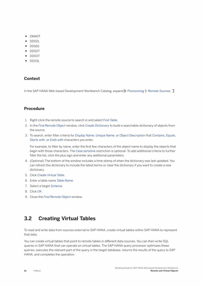
● DM40T● DD02L● DD16S● DD02T● DD03T● DD03L
Context
In the SAP HANA Web-based Development Workbench Catalog, expand Provisioning Remote Sources.
Procedure
1. Right-click the remote source to search in and select Find Table.2. In the Find Remote Object window, click Create Dictionary to build a searchable dictionary of objects from
the source.3. To search, enter filter criteria for Display Name, Unique Name, or Object Description that Contains, Equals,
Starts with, or Ends with characters you enter.
For example, to filter by name, enter the first few characters of the object name to display the objects that begin with those characters. The Case sensitive restriction is optional. To add additional criteria to further filter the list, click the plus sign and enter any additional parameters.
4. (Optional) The bottom of the window includes a time stamp of when the dictionary was last updated. You can refresh the dictionary to include the latest terms or clear the dictionary if you want to create a new dictionary.
5. Click Create Virtual Table.6. Enter a table name Table Name.7. Select a target Schema.8. Click OK.9. Close the Find Remote Object window.
3.2 Creating Virtual Tables
To read and write data from sources external to SAP HANA, create virtual tables within SAP HANA to represent that data.
You can create virtual tables that point to remote tables in different data sources. You can then write SQL queries in SAP HANA that can operate on virtual tables. The SAP HANA query processor optimizes these queries, executes the relevant part of the query in the target database, returns the results of the query to SAP HANA, and completes the operation.
10 PUBLICModeling Guide for SAP HANA Web-based Development Workbench
Remote and Virtual Objects
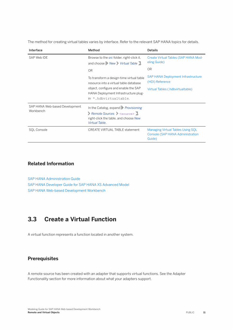
The method for creating virtual tables varies by interface. Refer to the relevant SAP HANA topics for details.
Interface Method Details
SAP Web IDE Browse to the src folder, right-click it,
and choose New Virtual Table .
OR
To transform a design-time virtual table resource into a virtual table database object, configure and enable the SAP HANA Deployment Infrastructure plug-in *.hdbvirtualtable.
Create Virtual Tables (SAP HANA Modeling Guide)
OR
SAP HANA Deployment Infrastructure (HDI) Reference
Virtual Tables (.hdbvirtualtable)
SAP HANA Web-based Development Workbench
In the Catalog, expand Provisioning
Remote Sources <source> , right-click the table, and choose New Virtual Table.
SQL Console CREATE VIRTUAL TABLE statement Managing Virtual Tables Using SQL Console (SAP HANA Administration Guide)
Related Information
SAP HANA Administration GuideSAP HANA Developer Guide for SAP HANA XS Advanced ModelSAP HANA Web-based Development Workbench
3.3 Create a Virtual Function
A virtual function represents a function located in another system.
Prerequisites
A remote source has been created with an adapter that supports virtual functions. See the Adapter Functionality section for more information about what your adapters support.
Modeling Guide for SAP HANA Web-based Development WorkbenchRemote and Virtual Objects PUBLIC 11
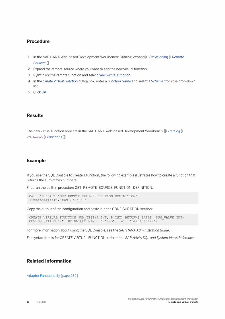
Procedure
1. In the SAP HANA Web-based Development Workbench: Catalog, expand Provisioning Remote Sources .
2. Expand the remote source where you want to add the new virtual function.3. Right-click the remote function and select New Virtual Function.4. In the Create Virtual Function dialog box, enter a Function Name and select a Schema from the drop-down
list.5. Click OK.
Results
The new virtual function appears in the SAP HANA Web-based Development Workbench: Catalog<Schema> Functions .
Example
If you use the SQL Console to create a function, the following example illustrates how to create a function that returns the sum of two numbers:
First run the built-in procedure GET_REMOTE_SOURCE_FUNCTION_DEFINITION:
CALL "PUBLIC"."GET_REMOTE_SOURCE_FUNCTION_DEFINITION" ('testAdapter','sum',?,?,?);
Copy the output of the configuration and paste it in the CONFIGURATION section:
CREATE VIRTUAL FUNCTION SUM_TEST(A INT, B INT) RETURNS TABLE (SUM_VALUE INT) CONFIGURATION '{"__DP_UNIQUE_NAME__":"sum"}' AT "testAdapter";
For more information about using the SQL Console, see the SAP HANA Administration Guide.
For syntax details for CREATE VIRTUAL FUNCTION, refer to the SAP HANA SQL and System Views Reference.
Related Information
Adapter Functionality [page 235]
12 PUBLICModeling Guide for SAP HANA Web-based Development Workbench
Remote and Virtual Objects

3.4 Virtual Procedures
For remote sources using SAP HANA smart data integration adapters, use a virtual procedure to execute a stored procedure in a remote system.
A virtual procedure in SAP HANA represents a stored procedure in a remote system. A virtual procedure can be invoked in SAP HANA like any other local procedure, but the execution of the stored procedure occurs in the remote system.
NoteNot all adapters support virtual procedures. See the "Adapter Functionality" section for more information about what your adapters support.
When you browse a remote source that was created with an adapter that supports virtual procedures, the adapter retrieves the list of stored procedures from the remote system. When you create a virtual procedure, the adapter imports the definition of the stored procedure from the remote system.
When you invoke the corresponding virtual procedure in SAP HANA, that invokes the stored procedure in the remote system. Invoke virtual procedures using the CALL SQL statement. You can also invoke a virtual procedure using a Procedure node in a flowgraph.
Related Information
Create a Virtual Procedure [page 13]
Procedure [page 202]CALL Statement (Procedural) (SAP HANA SQL and System Views Reference)Virtual Procedure Support with IBM DB2 [page 269]Virtual Procedure Support with Oracle [page 290]Virtual Procedure Support with Microsoft SQL Server [page 279]Adapter Functionality [page 235]
3.4.1 Create a Virtual Procedure
This task describes how to use the SAP HANA Web-based Development Workbench to create a virtual procedure.
Prerequisites
A remote source has been created with an adapter that supports virtual procedures. See the "Adapter Functionality" section for more information about what your adapters support.
Modeling Guide for SAP HANA Web-based Development WorkbenchRemote and Virtual Objects PUBLIC 13
Context
A virtual procedure represents a procedure or stored procedure located in another system. To invoke a stored procedure from another system in SAP HANA, you create a virtual procedure for that stored procedure, then invoke it either using the CALL SQL statement or in a flowgraph using the Procedure node.
For an example of creating a virtual procedure using the SQL console, see the topic "CREATE VIRTUAL PROCEDURE [Smart Data Integration]" in the SAP HANA SQL and System Views Reference. That guide also has the complete syntax details for the SAP HANA CREATE VIRTUAL PROCEDURE statement (Procedural). For more information about using the SQL console, see the SAP HANA Administration Guide.
Procedure
1. In the SAP HANA Web-based Development Workbench: Catalog, expand Provisioning Remote Sources .
2. Expand the remote source where you want to add the new virtual procedure.3. Right-click the remote procedure and select New Virtual Procedure.4. In the Create Virtual Procedure dialog box, enter a Procedure Name and select a Schema from the drop-
down list.5. Click OK.
Results
The new virtual procedure appears in the SAP HANA Web-based Development Workbench: Catalog ><Schema> > Procedures.
Related Information
Virtual Procedures [page 13]CREATE VIRTUAL PROCEDURE Statement (Procedural) (SAP HANA SQL and System Views Reference)CREATE VIRTUAL PROCEDURE Statement [Smart Data Integration]CALL Statement (Procedural) (SAP HANA SQL and System Views Reference)SAP HANA Administration Guide
14 PUBLICModeling Guide for SAP HANA Web-based Development Workbench
Remote and Virtual Objects
4 Replicating Data Using a Replication Task
Replicate data from several objects in a remote source to tables in SAP HANA using the Replication Editor in SAP HANA Web-based Development Workbench.
To replicate data from objects in a remote source into tables in SAP HANA, you must configure the replication process by creating an .hdbreptask file, which opens a file specific to the Replication Editor.
Before using the Replication Editor, you must have the proper rights to use the editor. See your system administrator to assign appropriate permissions. You must also have the run-time objects set up as described in the "SAP HANA Web-based Development Workbench: Catalog" chapter of the SAP HANA Developer Guide.
NoteThe Web-based Editor tool is available on the SAP HANA XS web server at the following URL: http://<WebServerHost>:80<SAPHANAInstance>/sap/hana/ide/editor.
After the .hdbreptask has been configured, activate it to generate a stored procedure, a remote subscription, one or more virtual tables for objects that you want to replicate, and target tables. Be sure to clear the Initial load only option to create the remote subscription. When the stored procedure is called, an initial load runs. When real time is enabled, the system automatically distributes subsequent changes.
DDL changes to source tables that are associated with a replication task propagate to SAP HANA so that the same changes apply to the SAP HANA target tables.
See the SAP HANA Smart Data Integration and SAP HANA Smart Data Quality Administration Guide for information about monitoring and processing remote subscriptions for real-time replication tasks.
Related Information
Create a Replication Task [page 16]Add a Target Column [page 22]Edit a Target Column [page 23]Delete a Target Column [page 23]Replication Behavior Options for Objects in Replication Tasks [page 24]Load Behavior Options for Targets in Replication Tasks [page 26]Partition Data in a Replication Task [page 29]Use Changed-Data Capture and Custom Parameters [page 33]Save and Execute a Replication Task [page 34]Force Reactivate Design Time Object [page 36]
Modeling Guide for SAP HANA Web-based Development WorkbenchReplicating Data Using a Replication Task PUBLIC 15
4.1 Create a Replication Task
A replication task retrieves data from one or more objects in a single remote source and populates one or more tables in SAP HANA.
Prerequisites
Before using the Replication Editor, you must have the proper rights to use the editor. For example, you must have the ALTER Object privilege on the remote source where you'll be searching. See your system administrator to be assigned appropriate permissions.
Context
Columns that you do not map as inputs to a replication task or flowgraph are not sent over the network for processing by SAP HANA. Excluding columns as inputs can improve performance, for example if they contain large object types. You can enhance security by excluding columns that, for example, include sensitive data such as passwords.
Procedure
1. In SAP HANA Web-based Development Workbench, highlight a package from the content pane and right-click. Choose New Replication Task .
2. Enter a file name and then click Create.3. In Remote Source, select the source data location from the dropdown list.
NoteIf the list is empty, verify that you have the correct permissions to the remote source.
4. In Target Schema, select the schema for the target table.5. In Virtual Table Schema, select the schema for the virtual table.6. Select whether to use the package prefix for the virtual and/or target tables. For example, if your virtual
table name is customer_demo, and you enable the Virtual Table option, the output would be "VT_customer_demo". The prefix is defined in the Source Virtual Table Prefix. You must set this option when the virtual table and the target table are the same.
7. (Optional) In the Source Virtual Table Prefix option, enter some identifying letters or numbers to help you label the virtual table. You might want a prefix to identify where the data came from or the type of information that it contains.
8. To include one or more tables in the replication task, click Add Objects.9. In the Select Remote Objects window, you can browse to or search for the objects. You can use Shift-click
or Ctrl-click to select multiple objects.
16 PUBLICModeling Guide for SAP HANA Web-based Development Workbench
Replicating Data Using a Replication Task
○ To browse for the object, expand the nodes as necessary and select the objects.○ To search for an object, click Create Dictionary to build a searchable dictionary of objects from the
source.
NoteYou need to create the dictionary only the first time you search for an object. It is automatically available after the first search.
Enter the Filter By criteria for Display Name, Unique Name, or Object Description that Contains, Equals, Starts with, or Ends with characters you enter.For example, to filter by name, enter the first few characters of the object name to display the objects that begin with those characters. The Case sensitive restriction is optional. To add additional criteria to further filter the list, click the plus sign and enter the additional parameters.The bottom of this interface includes a time stamp for when the dictionary was last updated. You can refresh or clear the dictionary here.
10. (Optional) Enter a prefix in the Target Name Prefix option. For example, you might want the prefix to be ADDR_ if the output table contains address data. The rest of the table name is the same as the remote object name. You can change the entire name on the main editing page, if necessary.
11. (Optional) Configure the Replication Behavior for the table. You can choose to perform a combination of initial load, real-time replication, and table-level structure replication depending on whether changed-data capture (CDC) is supported and whether you are using a table or virtual table.
Option Description
Initial load only Performs a one-time data load without any real-time replication. Always available.
Initial + Realtime Performs the initial data load and enables real-time replication. Available when CDC is supported. For tables and virtual tables.
Realtime Enables real-time replication without performing an initial data load. Available when CDC is supported. For tables and virtual tables.
No data transfer Replicates only the object structure without transferring any data. Always available.
Initial + realtime with structure Performs the initial data load, enables real-time replication, and tracks object-level changes. Available when CDC is supported and for tables.
Realtime only with structure Enables real-time replication and tracks object-level changes without performing an initial data load. Available when CDC is supported and for tables.
12. Click OK to close the Select Remote Objects dialog. The following information is included in the table.
Column Name Description
Source Remote Object Shows the name of the remote source and the table selected within the remote source.
Source Virtual Table Shows the name of the table to be created in SAP HANA after Save and Activation.
Target Name (Remote Source, Remote Object)
Shows the name of the target created in SAP HANA. You can choose whether to create a new or use an existing table or virtual table. See the next step.
Modeling Guide for SAP HANA Web-based Development WorkbenchReplicating Data Using a Replication Task PUBLIC 17
Column Name Description
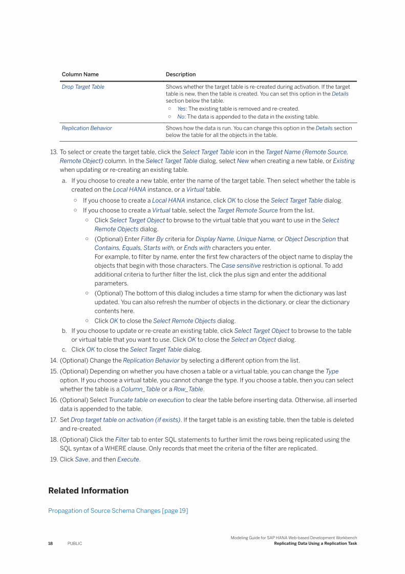
Drop Target Table Shows whether the target table is re-created during activation. If the target table is new, then the table is created. You can set this option in the Details section below the table.○ Yes: The existing table is removed and re-created.○ No: The data is appended to the data in the existing table.
Replication Behavior Shows how the data is run. You can change this option in the Details section below the table for all the objects in the table.
13. To select or create the target table, click the Select Target Table icon in the Target Name (Remote Source, Remote Object) column. In the Select Target Table dialog, select New when creating a new table, or Existing when updating or re-creating an existing table.a. If you choose to create a new table, enter the name of the target table. Then select whether the table is
created on the Local HANA instance, or a Virtual table.○ If you choose to create a Local HANA instance, click OK to close the Select Target Table dialog.○ If you choose to create a Virtual table, select the Target Remote Source from the list.
○ Click Select Target Object to browse to the virtual table that you want to use in the Select Remote Objects dialog.
○ (Optional) Enter Filter By criteria for Display Name, Unique Name, or Object Description that Contains, Equals, Starts with, or Ends with characters you enter.For example, to filter by name, enter the first few characters of the object name to display the objects that begin with those characters. The Case sensitive restriction is optional. To add additional criteria to further filter the list, click the plus sign and enter the additional parameters.
○ (Optional) The bottom of this dialog includes a time stamp for when the dictionary was last updated. You can also refresh the number of objects in the dictionary, or clear the dictionary contents here.
○ Click OK to close the Select Remote Objects dialog.b. If you choose to update or re-create an existing table, click Select Target Object to browse to the table
or virtual table that you want to use. Click OK to close the Select an Object dialog.c. Click OK to close the Select Target Table dialog.
14. (Optional) Change the Replication Behavior by selecting a different option from the list.15. (Optional) Depending on whether you have chosen a table or a virtual table, you can change the Type
option. If you choose a virtual table, you cannot change the type. If you choose a table, then you can select whether the table is a Column_Table or a Row_Table.
16. (Optional) Select Truncate table on execution to clear the table before inserting data. Otherwise, all inserted data is appended to the table.
17. Set Drop target table on activation (if exists). If the target table is an existing table, then the table is deleted and re-created.
18. (Optional) Click the Filter tab to enter SQL statements to further limit the rows being replicated using the SQL syntax of a WHERE clause. Only records that meet the criteria of the filter are replicated.
19. Click Save, and then Execute.
Related Information
Propagation of Source Schema Changes [page 19]
18 PUBLICModeling Guide for SAP HANA Web-based Development Workbench
Replicating Data Using a Replication Task
Add a Target Column [page 22]Edit a Target Column [page 23]Delete a Target Column [page 23]Replication Behavior Options for Objects in Replication Tasks [page 24]Load Behavior Options for Target Tables [page 26]Activate and Execute a Replication Task [page 34]
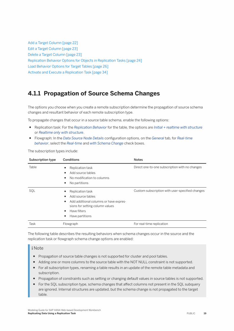
4.1.1 Propagation of Source Schema Changes
The options you choose when you create a remote subscription determine the propagation of source schema changes and resultant behavior of each remote subscription type.
To propagate changes that occur in a source table schema, enable the following options:
● Replication task: For the Replication Behavior for the table, the options are Initial + realtime with structure or Realtime only with structure.
● Flowgraph: In the Data Source Node Details configuration options, on the General tab, for Real-time behavior, select the Real-time and with Schema Change check boxes.
The subscription types include:
Subscription type Conditions Notes
Table ● Replication task● Add source tables● No modification to columns● No partitions
Direct one-to-one subscription with no changes
SQL ● Replication task● Add source tables● Add additional columns or have expres
sions for setting column values● Have filters● Have partitions
Custom subscription with user-specified changes
Task Flowgraph For real-time replication
The following table describes the resulting behaviors when schema changes occur in the source and the replication task or flowgraph schema change options are enabled:
Note● Propagation of source table changes is not supported for cluster and pool tables.● Adding one or more columns to the source table with the NOT NULL constraint is not supported.● For all subscription types, renaming a table results in an update of the remote table metadata and
subscription.● Propagation of constraints such as setting or changing default values in source tables is not supported.● For the SQL subscription type, schema changes that affect columns not present in the SQL subquery
are ignored. Internal structures are updated, but the schema change is not propagated to the target table.
Modeling Guide for SAP HANA Web-based Development WorkbenchReplicating Data Using a Replication Task PUBLIC 19

● If you specify the optional WITH RESTRICTED SCHEMA CHANGES clause instead of WITH SCHEMA CHANGES, schema changes are propagated only to the SAP HANA virtual table and not the remote subscription target table.
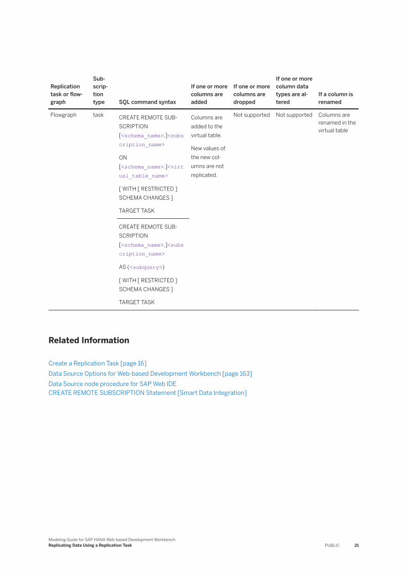
Replication task or flowgraph
Subscription type SQL command syntax
If one or more columns are added
If one or more columns are dropped
If one or more column data types are altered
If a column is renamed
Replication Task
Table CREATE REMOTE SUBSCRIPTION [<schema_name>.]<subscription_name>
ON [<schema_name>.]<virtual_table_name>
[ WITH [ RESTRICTED ] SCHEMA CHANGES ]
TARGET TABLE
Columns are added to the target and virtual tables.
New values are replicated in the new column(s) in the target table.
Columns are dropped from the target and virtual tables.
Data types are altered in the target and virtual tables.
Columns are renamed in the target and virtual tables.
Replication Task
SQL CREATE REMOTE SUBSCRIPTION [<schema_name>.]<subscription_name>
AS (<subquery>)
[ WITH [ RESTRICTED ] SCHEMA CHANGES ]
TARGET TABLE
Columns are added to the target and virtual tables
If a single-level subquery is specified, the values in the new columns replicate.
If a multilevel subquery is specified, a NULL value is assigned to the data for the new columns.
Not supported Data types are altered in the target and virtual tables.
Columns are renamed in the target and virtual tables.
20 PUBLICModeling Guide for SAP HANA Web-based Development Workbench
Replicating Data Using a Replication Task
Replication task or flowgraph
Subscription type SQL command syntax
If one or more columns are added
If one or more columns are dropped
If one or more column data types are altered
If a column is renamed
Flowgraph task CREATE REMOTE SUBSCRIPTION [<schema_name>.]<subscription_name>
ON [<schema_name>.]<virtual_table_name>
[ WITH [ RESTRICTED ] SCHEMA CHANGES ]
TARGET TASK
Columns are added to the virtual table.
New values of the new columns are not replicated.
Not supported Not supported Columns are renamed in the virtual table
CREATE REMOTE SUBSCRIPTION [<schema_name>.]<subscription_name>
AS (<subquery>)
[ WITH [ RESTRICTED ] SCHEMA CHANGES ]
TARGET TASK
Related Information
Create a Replication Task [page 16]Data Source Options for Web-based Development Workbench [page 163]Data Source node procedure for SAP Web IDECREATE REMOTE SUBSCRIPTION Statement [Smart Data Integration]
Modeling Guide for SAP HANA Web-based Development WorkbenchReplicating Data Using a Replication Task PUBLIC 21

4.2 Add a Target Column
Using the Replication Editor, you can add a new column or an existing column (from a remote object) to the target table.
Procedure
1. From the Replication Editor, on the Target Columns tab, click Add.2. Choose whether to create a column or to include a column from a remote object.
○ From remote object: Browse to a source and table and choose the column you replicated in the virtual table:1. Select the column name.2. Indicate if this column is part of the primary key.3. Click OK.4. Rename the column.5. Enter the projection.
○ From scratch: Complete the following steps to create a column. Then, you can enter SQL statements in the Filter tab to set the value of the target column during replication. You can use any of the SAP HANA SQL functions. See the SAP Hana SQL and System Views Reference.1. Enter the name of the column.2. Select the data type. For example varchar, decimal and so on.3. Enter the number of characters allowed in the column.4. Enter the projection, which is the mapped name, of the column.
NoteThe projection can be any one of the following:○ Column: Enter the name of the source column in double quotes, for example "APJ_SALES".○ String literal: Enter the string as a value in single quotes, for example 'ERPCLNT800'.○ SQL expression: For example "firstname" + "lastname"
5. Select is nullable if the value can be empty.6. Select is part of the primary key if the data in the column uniquely identifies each record in a table.7. Select OK.
Related Information
Create a replication task [page 16]
22 PUBLICModeling Guide for SAP HANA Web-based Development Workbench
Replicating Data Using a Replication Task
4.3 Edit a Target Column
Modify the column to correct the data or to make it more accurate or useful.
Context
For example, if you are using a Social Security number as a part of a primary key, and you need to stop using it for the primary key, you can edit the column to unselect the option. To edit a column:
Procedure
1. Select the column.2. Click Edit.3. Change the data type, length, projection, nullable, or primary key options as needed.4. Click OK.
4.4 Delete a Target Column
Remove a column to no longer use it in a flowgraph.
Procedure
1. Select the column.2. Click Delete.3. Confirm your deletion, and then click OK.
Modeling Guide for SAP HANA Web-based Development WorkbenchReplicating Data Using a Replication Task PUBLIC 23
4.5 Replication Behavior Options for Objects in Replication Tasks
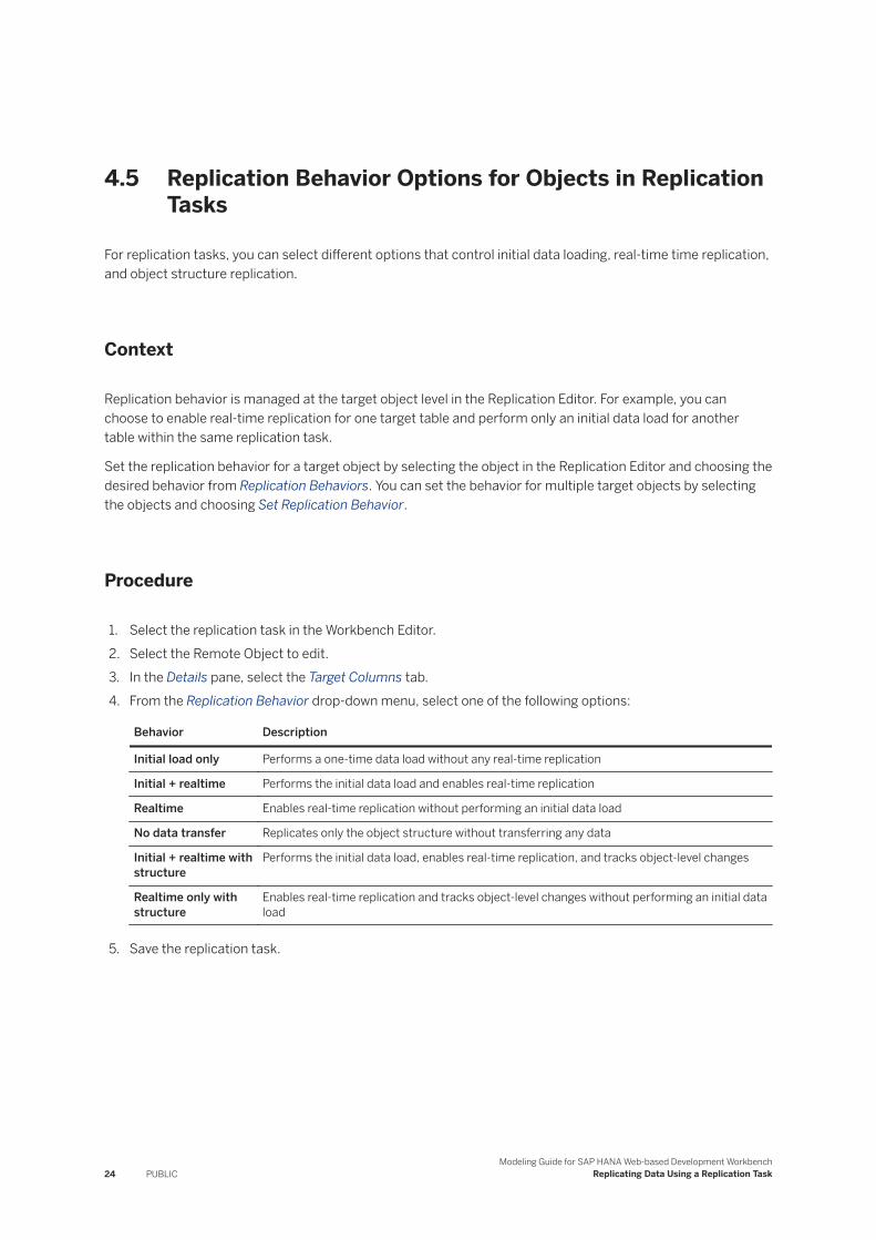
For replication tasks, you can select different options that control initial data loading, real-time time replication, and object structure replication.
Context
Replication behavior is managed at the target object level in the Replication Editor. For example, you can choose to enable real-time replication for one target table and perform only an initial data load for another table within the same replication task.
Set the replication behavior for a target object by selecting the object in the Replication Editor and choosing the desired behavior from Replication Behaviors. You can set the behavior for multiple target objects by selecting the objects and choosing Set Replication Behavior.
Procedure
1. Select the replication task in the Workbench Editor.2. Select the Remote Object to edit.3. In the Details pane, select the Target Columns tab.4. From the Replication Behavior drop-down menu, select one of the following options:
Behavior Description
Initial load only Performs a one-time data load without any real-time replication
Initial + realtime Performs the initial data load and enables real-time replication
Realtime Enables real-time replication without performing an initial data load
No data transfer Replicates only the object structure without transferring any data
Initial + realtime with structure
Performs the initial data load, enables real-time replication, and tracks object-level changes
Realtime only with structure
Enables real-time replication and tracks object-level changes without performing an initial data load
5. Save the replication task.
24 PUBLICModeling Guide for SAP HANA Web-based Development Workbench
Replicating Data Using a Replication Task
4.5.1 Support for Schema Change Replication
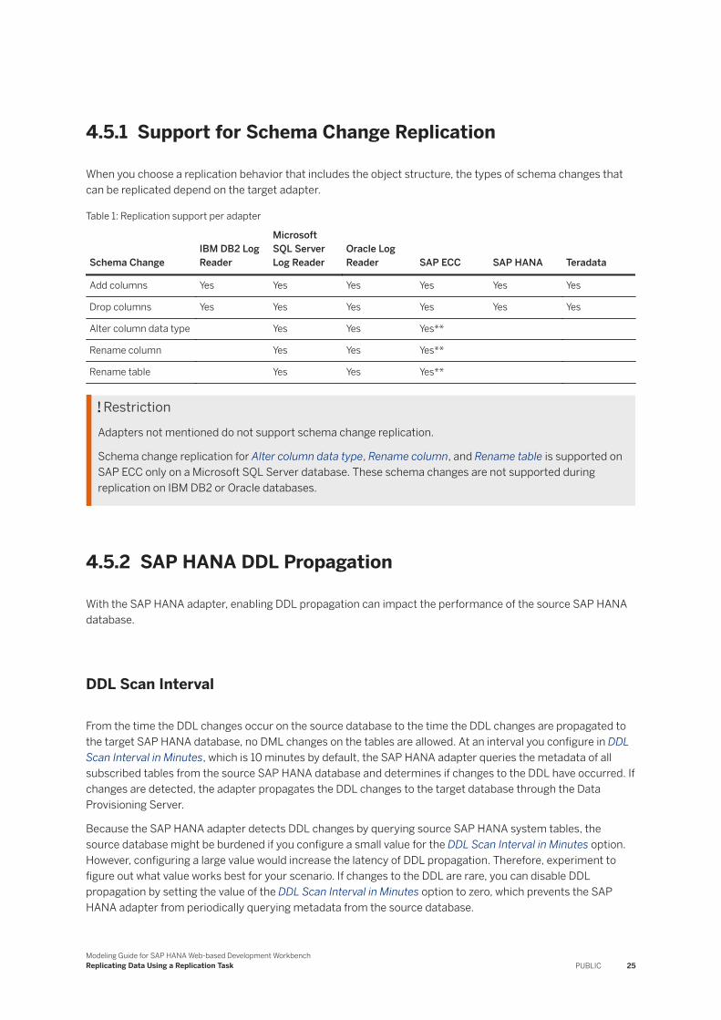
When you choose a replication behavior that includes the object structure, the types of schema changes that can be replicated depend on the target adapter.
Table 1: Replication support per adapter
Schema ChangeIBM DB2 Log Reader
Microsoft SQL Server Log Reader
Oracle Log Reader SAP ECC SAP HANA Teradata
Add columns Yes Yes Yes Yes Yes Yes
Drop columns Yes Yes Yes Yes Yes Yes
Alter column data type Yes Yes Yes**
Rename column Yes Yes Yes**
Rename table Yes Yes Yes**
RestrictionAdapters not mentioned do not support schema change replication.
Schema change replication for Alter column data type, Rename column, and Rename table is supported on SAP ECC only on a Microsoft SQL Server database. These schema changes are not supported during replication on IBM DB2 or Oracle databases.
4.5.2 SAP HANA DDL Propagation
With the SAP HANA adapter, enabling DDL propagation can impact the performance of the source SAP HANA database.
DDL Scan Interval
From the time the DDL changes occur on the source database to the time the DDL changes are propagated to the target SAP HANA database, no DML changes on the tables are allowed. At an interval you configure in DDL Scan Interval in Minutes, which is 10 minutes by default, the SAP HANA adapter queries the metadata of all subscribed tables from the source SAP HANA database and determines if changes to the DDL have occurred. If changes are detected, the adapter propagates the DDL changes to the target database through the Data Provisioning Server.
Because the SAP HANA adapter detects DDL changes by querying source SAP HANA system tables, the source database might be burdened if you configure a small value for the DDL Scan Interval in Minutes option. However, configuring a large value would increase the latency of DDL propagation. Therefore, experiment to figure out what value works best for your scenario. If changes to the DDL are rare, you can disable DDL propagation by setting the value of the DDL Scan Interval in Minutes option to zero, which prevents the SAP HANA adapter from periodically querying metadata from the source database.
Modeling Guide for SAP HANA Web-based Development WorkbenchReplicating Data Using a Replication Task PUBLIC 25
Limitation
Remember that during the time period between when DDL changes occur on the source database and when they are replicated to the target SAP HANA database, there must be no DML changes on the subscribed source tables. Replicating DDL changes triggers the SAP HANA adapter to update triggers and shadow tables on the changed source tables by dropping and then re-creating them. Errors might result if any data is inserted, updated, or deleted on the source tables during this time period.
Related Information
SAP HANA Remote Source Configuration
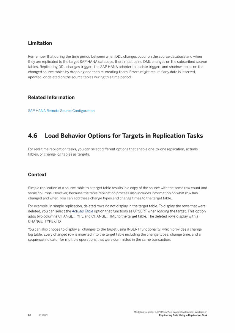
4.6 Load Behavior Options for Targets in Replication Tasks
For real-time replication tasks, you can select different options that enable one-to-one replication, actuals tables, or change log tables as targets.
Context
Simple replication of a source table to a target table results in a copy of the source with the same row count and same columns. However, because the table replication process also includes information on what row has changed and when, you can add these change types and change times to the target table.
For example, in simple replication, deleted rows do not display in the target table. To display the rows that were deleted, you can select the Actuals Table option that functions as UPSERT when loading the target. This option adds two columns CHANGE_TYPE and CHANGE_TIME to the target table. The deleted rows display with a CHANGE_TYPE of D.
You can also choose to display all changes to the target using INSERT functionality, which provides a change log table. Every changed row is inserted into the target table including the change types, change time, and a sequence indicator for multiple operations that were committed in the same transaction.
26 PUBLICModeling Guide for SAP HANA Web-based Development Workbench
Replicating Data Using a Replication Task
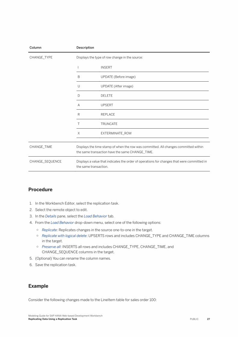
Column Description
CHANGE_TYPE Displays the type of row change in the source:
I INSERT
B UPDATE (Before image)
U UPDATE (After image)
D DELETE
A UPSERT
R REPLACE
T TRUNCATE
X EXTERMINATE_ROW
CHANGE_TIME Displays the time stamp of when the row was committed. All changes committed within the same transaction have the same CHANGE_TIME.
CHANGE_SEQUENCE Displays a value that indicates the order of operations for changes that were committed in the same transaction.
Procedure
1. In the Workbench Editor, select the replication task.2. Select the remote object to edit.3. In the Details pane, select the Load Behavior tab.4. From the Load Behavior drop-down menu, select one of the following options:
○ Replicate: Replicates changes in the source one-to-one in the target.○ Replicate with logical delete: UPSERTS rows and includes CHANGE_TYPE and CHANGE_TIME columns
in the target.○ Preserve all: INSERTS all rows and includes CHANGE_TYPE, CHANGE_TIME, and
CHANGE_SEQUENCE columns in the target.5. (Optional) You can rename the column names.6. Save the replication task.
Example
Consider the following changes made to the LineItem table for sales order 100:
Modeling Guide for SAP HANA Web-based Development WorkbenchReplicating Data Using a Replication Task PUBLIC 27
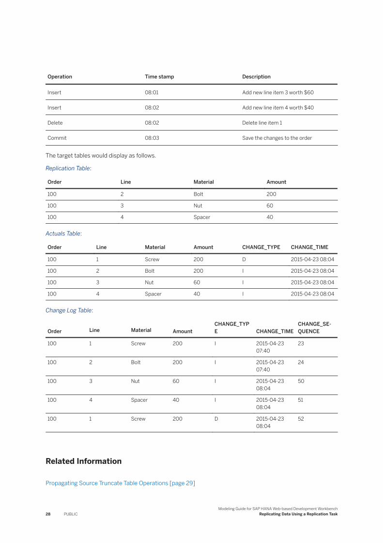
Operation Time stamp Description
Insert 08:01 Add new line item 3 worth $60
Insert 08:02 Add new line item 4 worth $40
Delete 08:02 Delete line item 1
Commit 08:03 Save the changes to the order
The target tables would display as follows.
Replication Table:
Order Line Material Amount
100 2 Bolt 200
100 3 Nut 60
100 4 Spacer 40
Actuals Table:
Order Line Material Amount CHANGE_TYPE CHANGE_TIME
100 1 Screw 200 D 2015-04-23 08:04
100 2 Bolt 200 I 2015-04-23 08:04
100 3 Nut 60 I 2015-04-23 08:04
100 4 Spacer 40 I 2015-04-23 08:04
Change Log Table:
Order Line Material AmountCHANGE_TYPE CHANGE_TIME
CHANGE_SEQUENCE
100 1 Screw 200 I 2015-04-23 07:40
23
100 2 Bolt 200 I 2015-04-23 07:40
24
100 3 Nut 60 I 2015-04-23 08:04
50
100 4 Spacer 40 I 2015-04-23 08:04
51
100 1 Screw 200 D 2015-04-23 08:04
52
Related Information
Propagating Source Truncate Table Operations [page 29]
28 PUBLICModeling Guide for SAP HANA Web-based Development Workbench
Replicating Data Using a Replication Task
Load Behavior Options for Targets in the Flowgraph [page 157]
4.6.1 Propagating Source Truncate Table Operations
Under some circumstances, you can propagate your source table truncation operations to the target table.
By default, if SAP HANA receives a truncated row, we log an exception stating that truncation isn’t supported and that you should ignore the exception. The solution to this issue is to enable a dpserver.ini file parameter by setting dataprovisioning > enable_propagate_truncate_table = 'true'.
The truncate table propagation operation is supported for the following target types (reptask or SQL-based):
● Target Table: All rows are deleted.● Target Table with logical delete: The change type column for all of the not-deleted rows are set to D, and the
change time is set to the latest timestamp.● Target Table with history preserving: A new row is inserted into the target table with a change type column
value of P, indicating a pruning of the table data. The change time and change sequence is set to the latest values. None of the existing rows are modified.
NoteThis operation isn’t supported for task (flowgraph) or procedure target types. Also, this operation is supported on most adapters except for those using trigger-based replication such as SAP HANA, Oracle, or Microsoft SQL Server.
4.7 Partition Data in a Replication Task
Partitioning data can be helpful when you are initially loading a large data set, because it can improve performance and assist in managing memory usage.
Context
NotePartitioning data in a replication task applies to SAP HANA Web-based Development Workbench only.
Data partitioning separates large data sets into smaller sets based on defined criteria. Some common reasons for partitioning include:
● You receive “out of memory” errors when you load the data.● You have reached the limit for the maximum number of rows within a column store.● You want the performance to be faster.
You can partition data for virtual tables in two ways: at the Input level, or at the Task level. Input partitioning only affects the process of reading the remote source data. Task level partitioning partitions the entire replication
Modeling Guide for SAP HANA Web-based Development WorkbenchReplicating Data Using a Replication Task PUBLIC 29
task, from reading the data from the remote source to loading the data in the target object and everything in between. These partitions can run in serial or in parallel.
Currently, SAP HANA has a limitation where it does not process data sets of two billion or more rows. If your data contains more than two billion or more rows, then you must partition the data so that each partition contains less than two billion rows.
Typically, you see a benefit of using task level partitioning only with extremely large data sets. You can set the number of parallel partitions that are processed simultaneously. The transformation and loading to the target is done per partition, whereas input partitioning is done only for the remote source, and you cannot set the number of parallel partitions.
Procedure
1. Create the replication task and add an object.2. In the Details section, click the Partitions tab.3. Choose one of the following options:
○ Extract Only: Partitioning is done when loading the remote source data only. You cannot choose the number of parallel partitions.
○ Extract, Transform & Load: Partitioning is done for the entire flow, from loading the remote source to writing to the output table.
4. If you chose Task partitioning, set the Number of Parallel Partitions. For example, if you have five partitions, and you set the number of parallel partitions to 2, then partitions 1 and 2 are run together. When partition 1 or 2 completes processing, then partition 3 starts running, and so on. In general, the more partitions that you run in parallel, the faster the data loads. However, if there are memory issues, then data may not load because there are too many parallel partitions set. When this option is set to 1, then partitioning is run in a series beginning with the first partition. When that partition is finished, the second partition is started, and so on.
5. In the Attributes option, select the column whose data value you want to use for partitioning. For example, if you have a country column with European data, you might choose to partition data based on the values of Germany, France, Spain, and so on.
NoteWe recommend that when you partition the data, make sure that each partition contains approximately the same number of records.
6. Select the partition type that you want to use.
Option Description
List The data is divided into sets based on a list of values in a column. For example, if you want to partition France, Germany, and the United Kingdom, you enter ‘FR’, ‘DE’, ‘GB’ with single quotes around each value.
Range The data is divided into sets based on a range of data in the column. You need to enter only the ending value in the range. For example, the range of values can be 300. If this is an integer value, it includes all records from 0-299. (For a non-integer value, it includes values less than 300.) You could have a second partition that has the ending value of 900, which includes all records from 300-899.
30 PUBLICModeling Guide for SAP HANA Web-based Development Workbench
Replicating Data Using a Replication Task
Option Description
String value results are in alphabetical order. When using string values, make sure the data is surrounded by single quotation marks, for example, ‘NM’ for the state of New Mexico in the United States. Note that in the string value, the partition would not include the value 'NM'. In this example, it would include all US states from AK (Alaska) through NJ (New Jersey).
Custom Range The data is divided into sets based on a range of data in the column. You can enter the beginning and ending values in the range, or only the beginning or ending value. You can also set whether the minimum and maximum values are inclusive in the range. For example, if you are grouping the social media presense of 18-24 year olds inclusively, then those who are 18 and 24 (and all ages between 18 and 24) are included in the data. Whereas 18-24 exclusive means all those who are aged 19, 20, 21, 22, and 23 are counted.
Like the Range option, string values are in alphabetical order.
7. Click Add.8. Enter a partition name. For example, if you are partitioning on the country names, you might enter the
location of the country, such as Western Europe.9. Enter the Values that you want included in the partition. For example, you might enter ‘FR’, ‘PT’, ‘ES’, and
‘GB’ for the countries of France, Portugal, Spain, and United Kingdom. Click OK. Repeat the previous three steps to add more partitions. You must define a minimum of two partitions.
NoteIf you have additional values that do not apply to the partitions you created, the data will not be lost. The data will be replicated. For example, if you have the value 'DE' for Germany, those records are replicated even though they are not specified in a partition.
10. Click Save and continue setting up your replication task.
Example
List Partitioning Example
Let’s say that you have a table with European customers. You have hundreds of thousands of customers in Spain, France, and Germany, and tens of thousands of customers in Belgium, the Netherlands, and Denmark. You might set your partitions like this:
Partitioning: Task Number of parallel partitions: 2
Input Source: Euro_Data Partition type: List
Attribute: Country
Partition Name Value
Spain 'ES'
France 'FR'
Modeling Guide for SAP HANA Web-based Development WorkbenchReplicating Data Using a Replication Task PUBLIC 31
Partition Name Value
Germany 'DE'
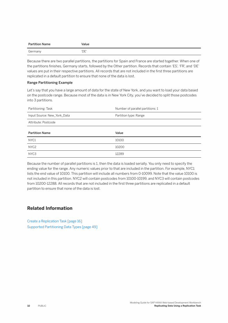
Because there are two parallel partitions, the partitions for Spain and France are started together. When one of the partitions finishes, Germany starts, followed by the Other partition. Records that contain ‘ES’, ‘FR’, and ‘DE’ values are put in their respective partitions. All records that are not included in the first three partitions are replicated in a default partition to ensure that none of the data is lost.
Range Partitioning Example
Let’s say that you have a large amount of data for the state of New York, and you want to load your data based on the postcode range. Because most of the data is in New York City, you’ve decided to split those postcodes into 3 partitions.
Partitioning: Task Number of parallel partitions: 1
Input Source: New_York_Data Partition type: Range
Attribute: Postcode
Partition Name Value
NYC1 10100
NYC2 10200
NYC3 12289
Because the number of parallel partitions is 1, then the data is loaded serially. You only need to specify the ending value for the range. Any numeric values prior to that are included in the partition. For example, NYC1 lists the end value of 10100. This partition will include all numbers from 0-10099. Note that the value 10100 is not included in this partition. NYC2 will contain postcodes from 10100-10199, and NYC3 will contain postcodes from 10200-12288. All records that are not included in the first three partitions are replicated in a default partition to ensure that none of the data is lost.
Related Information
Create a Replication Task [page 16]Supported Partitioning Data Types [page 49]
32 PUBLICModeling Guide for SAP HANA Web-based Development Workbench
Replicating Data Using a Replication Task
4.8 Use Changed-Data Capture and Custom Parameters
Use changed-data capture and custom parameters to track the data that has changed.
Context
You might want to perform actions on data that has changed.
Typically, changed-data capture (CDC) is used when running in real-time mode. Custom parameters are used when running in batch mode. The available options and parameters are defined in the virtual object such as a calculation view; therefore, if you do not see changed-data capture or custom parameter options in your replication task or in the Input Type node, the virtual object does not have the options defined.
Let's say that you are streaming Twitter public data in real-time mode to learn the latest trends regarding a popular gadget named Gizmo. You want to gather all tweets about Gizmo and learn whether the product launch was a success in the eye of the attendees. Therefore, your administrator has set up a virtual table with the parameters Product and User. If you want data about the product only, you would enter a product value of Gizmo. If you specifically want data about Gizmo from an industry expert with the Twitter handle of TechEx3000, you would enter a Product value of Gizmo and a User value of TechEx3000.
Procedure
1. Access the CDC and custom parameters in the following ways:
○ In a replication task, select the remote source object, and select Custom Parameters or CDC Parameters.
○ In a flowgraph, click the Input Type node, and select the Parameters tab.2. For the available parameters, select or enter a value. When entering values for multiple parameters, note
that all of the value conditions must be met to output the data. If you have entered the values Gizmo and TechEx3000, the software outputs only those occurrences that have both values.
3. Click Save.
Modeling Guide for SAP HANA Web-based Development WorkbenchReplicating Data Using a Replication Task PUBLIC 33
4.9 Save and Execute a Replication Task
Activation generates the run-time objects necessary for data movement from one or many source tables to one or more target tables.
Context
The replication task creates the following run-time objects:
● Virtual tables: Generated in the specified virtual table schema.● Remote subscriptions: Generated in the schema selected for the virtual table.● Tasks: Generated in the same schema as the target table.● Views: Generated in the same schema as the virtual table.● Target tables: Populated with the content after execution.● Procedure: Generated in the schema of the target table, the procedure performs three functions:
1. Sets the remote subscription to the Queue status.2. Calls Start Task to perform the initial load of the data.3. Sets the remote subscription to the Distribute status. Any changes, additions, and deletions made to
the source data during the initial load update in the target system. Any changes to the source data thereafter update in real time to the target.
NoteThe remote subscription is only created when Initial load only is cleared.
Procedure
1. After the replication task is configured, click Save to activate it.
NoteA replication task should not be in the MAT_START_BEG_MARKER state for a long period of time; for example, if QUEUE finishes but DISTRIBUTE never runs. As soon as the initial load finishes, the DISTRIBUTE command should execute as soon as possible. Otherwise, replicated data continues to be queued against the replication and causes unnecessary data volume usage. This scenario slows down the overall replication when the subscription is eventually distributed. If such a replication is QUEUED but not needed later, RESET it as soon as possible.
2. Go to the Catalog view and navigate to the stored procedure you just created.
NoteYou can access the Catalog view on the SAP HANA XS Web server at the following URL http://<WebServerHost>:80<SAPHanaInstance>/sap/hana/xs/ide/catalog. Choose one of the following options to activate the replication task.
34 PUBLICModeling Guide for SAP HANA Web-based Development Workbench
Replicating Data Using a Replication Task
○ Right-click the stored procedure, and then select Invoke Procedure.○ To call the stored procedure, use the following SQL script:
CALL "<schema_name>"."<package_name>::<target_table_name>".START_REPLICATION
.
The replication begins. You can right-click and select Open Contents to view the data in the target table in the Catalog view.
NoteIf the replication task takes longer than 300 seconds to process, you might receive an error about the XMLHttpRequest failing. You can correct this issue by increasing the maximum run time option in the xsengin.ini file. Follow these steps:1. Log in to SAP HANA studio as a SYSTEM user.2. In the Systems view, right-click the name of your SAP HANA server and then choose
Configuration and Monitoring Open Administration .3. Click the Configuration tab.4. Select xsengine.ini.5. Expand httpserver.6. Click Add parameter.7. In the Assign Values to option, select System, and then select Next.8. In the Key option, enter max_request_runtime and then enter a value. For example, you might
enter 1200. The value is in seconds.9. Click Finish and then close the Configuration tab and execute the replication task again.
Results
You can use monitors available from the SAP HANA cockpit to monitor the results.
Related Information
Monitoring Data Provisioning in the SAP HANA Web-based Development WorkbenchSAP HANA SQL and System Views Reference
Modeling Guide for SAP HANA Web-based Development WorkbenchReplicating Data Using a Replication Task PUBLIC 35
4.10 Force Reactivate Design Time Object
Reactivate tasks when dependent task objects are deleted or deactivated.
Context
NoteThis topic applies to SAP HANA Web-based Development Workbench only.
There might be times when an object such as a table that is used by or was generated by a flowgraph or replication task is deleted or becomes deactivated. This object might be used by more than one flowgraph or replication task. Therefore, multiple tasks might be invalid. Follow the steps below to force the reactivation of design time objects and make them active again. During force reactivation, the selected flowgraphs, replication tasks, and supporting objects are removed and recreated with the same names.
NoteYou can reactivate multiple flowgraphs and replication tasks by multi-selecting those objects that need to be reactivated. The tasks can be inside separate project containers. Only previously activated design time objects can be reactivated. If you have multi-selected several objects and don't see the Force Reactivate option, you may have included a task or object that cannot be reactivated.
Before beginning, make sure that you have the appropriate permissions to view the dependent objects using _SYS_REPO_ACTIVE_OBJECTCROSSREF. You also need permission to process the force reactivation. These are the same permissions for executing a task. See your system administrator to be assigned the appropriate permissions.
Procedure
1. From the file explorer in Web-based Development Workbench Editor, expand the Content folder. Expand your packages and select one or more flowgraph or replication tasks.
2. Right-click and select Force Reactivate.A Confirmation window shows the list of objects associated with the tasks. During processing, these objects are dropped and recreated.
NoteYou can filter on the Name, Type, or File by clicking in the column header and entering text.
3. In the Confirmation window, click Proceed.The tasks are reactivated one at a time starting from the top of the list. Tasks that are successfully reactivated are shown in the status area. Any tasks that were scheduled to reactivate after an error are not reactivated. For example, if you have four tasks to reactivate and the reactivation fails on the third task,
36 PUBLICModeling Guide for SAP HANA Web-based Development Workbench
Replicating Data Using a Replication Task

then the third and fourth tasks are not reactivated. If the reactivation fails, an error message is shown in the status area.
If the reactivation fails, do the following:1. Refresh the file explorer. A backup file named <objectname>_<timestamp>_Backup.txt is shown
next to the original task.2. Delete the original task.3. Rename the Backup.txt file to the original flowgraph or replication task name.4. Follow the force reactivation steps again.
If nothing is displayed in the status after force reactivate has started, check the log files. Log out of Web-based Development Workbench, close the browser, and log in again to continue working.
Related Information
AuthorizationsActivating and Executing Task Flowgraphs and Replication Tasks
Modeling Guide for SAP HANA Web-based Development WorkbenchReplicating Data Using a Replication Task PUBLIC 37
5 Transforming Data
To transform data, create a flowgraph in the flowgraph editor using a variety of available transformation nodes, for example Join, Filter, Cleanse, and Aggregation.
Perform the following tasks when creating flowgraphs:
1. Planning for Data Transformation [page 38]Before you begin transforming data, ensure that you have the proper permissions, have created the virtual objects, and know which flowgraph editor to use.
2. Defining Flowgraph Behavior [page 39]Some flowgraph concepts and objects are set outside of the nodes.
3. Transforming Data Using SAP HANA Web-based Development Workbench [page 55]Use the flowgraph editor in SAP HANA Web-based Development Workbench to create flowgraphs to transform and virtualize data.
4. Save and Execute a Flowgraph [page 215]After your flowgraph is created and configured, activate it to create the run-time objects.
5. Force Reactivate Design Time Object [page 216]Reactivate tasks when dependent task objects are deleted or deactivated.
Related Information
5.1 Planning for Data Transformation
Before you begin transforming data, ensure that you have the proper permissions, have created the virtual objects, and know which flowgraph editor to use.
Permissions and Privileges
Work with your system administrator to ensure you have rights to perform the following functions. These are the minimum rights; you might need more.
● Create a task● Stop a task● Create a remote source● Add a virtual table
38 PUBLICModeling Guide for SAP HANA Web-based Development Workbench
Transforming Data
● Create a remote subscription● Create a flowgraph● Create a flowgraph of the type task● Create a replication task● Activate replication task● Activate flowgraph● Execute a stored procedure● Execute a task
NoteIn addition to these permissions, your system administrator must configure a grantor for your HDI container. For more information, see Configure a Grantor for the HDI Container.
For more information about permissions, see the Installation and Configuration Guide for SAP HANA Smart Data Integration and Smart Data Quality.
Virtual Objects
Typically a system administrator will create remote sources for you to use. After you have a remote source created, you can create virtual tables, functions, and procedures you can use when creating the flowgraph.
For more information about virtual objects, see Remote and Virtual Objects [page 9].
Parent topic: Transforming Data [page 38]
Next: Defining Flowgraph Behavior [page 39]
Related Information
Assign Roles and Privileges
5.2 Defining Flowgraph Behavior
Some flowgraph concepts and objects are set outside of the nodes.
For example, you can create variables that can be used throughout the flowgraph, and you can partition the data so that it will read, transform and load the data quicker. In addition, there is a common expression editor used in several of the nodes.
Add a Variable to the Flowgraph [page 40]Create variables to have more flexibility when activating a flowgraph.
Modeling Guide for SAP HANA Web-based Development WorkbenchTransforming Data PUBLIC 39

Partitioning Data in the Flowgraph [page 42]Partitioning data can be helpful when you are initially loading a large data set because it can improve performance. There are several ways to achieve partitioning.
Choosing the Run-time Behavior [page 50]When creating a flowgraph, you need to consider how you want it to be processed.
Importing an Agile Data Preparation Flowgraph [page 52]Import and configure a flowgraph originally created in SAP Agile Data Preparation.
Use the Expression Editor [page 54]The Expression Editor is available in the Aggregation, Case, Join, Lookup, Map Operation, Projection, and Table Comparison nodes.
Reserved Words [page 54]The following words have special meaning for Data Provisioning nodes.
Nodes Available for Real-time Processing [page 54]A list showing which nodes can be used in a real-time enabled flowgraph.
Parent topic: Transforming Data [page 38]
Previous: Planning for Data Transformation [page 38]
Next: Transforming Data Using SAP HANA Web-based Development Workbench [page 55]
Related Information
5.2.1 Add a Variable to the Flowgraph
Create variables to have more flexibility when activating a flowgraph.
Context
When you create variables, you can use them in nodes that accept them such as the Filter node and Aggregation nodes. For example, in a Filter node, you might want to process only those records for a certain country, such as Spain. You can create a variable for the country in the flowgraph properties. Then you can use the variable in the filter by surrounding the variable name with $$. For example,
"Filter1_Input"."COUNTRY" = $$COUNTRY_PARAM$$
The variables are provided at the time of execution, so you don't need to edit the flowgraph when you want to output data for Spain in one run and then Germany in another run, for example. Just change the variable for each run.
40 PUBLICModeling Guide for SAP HANA Web-based Development Workbench
Transforming Data
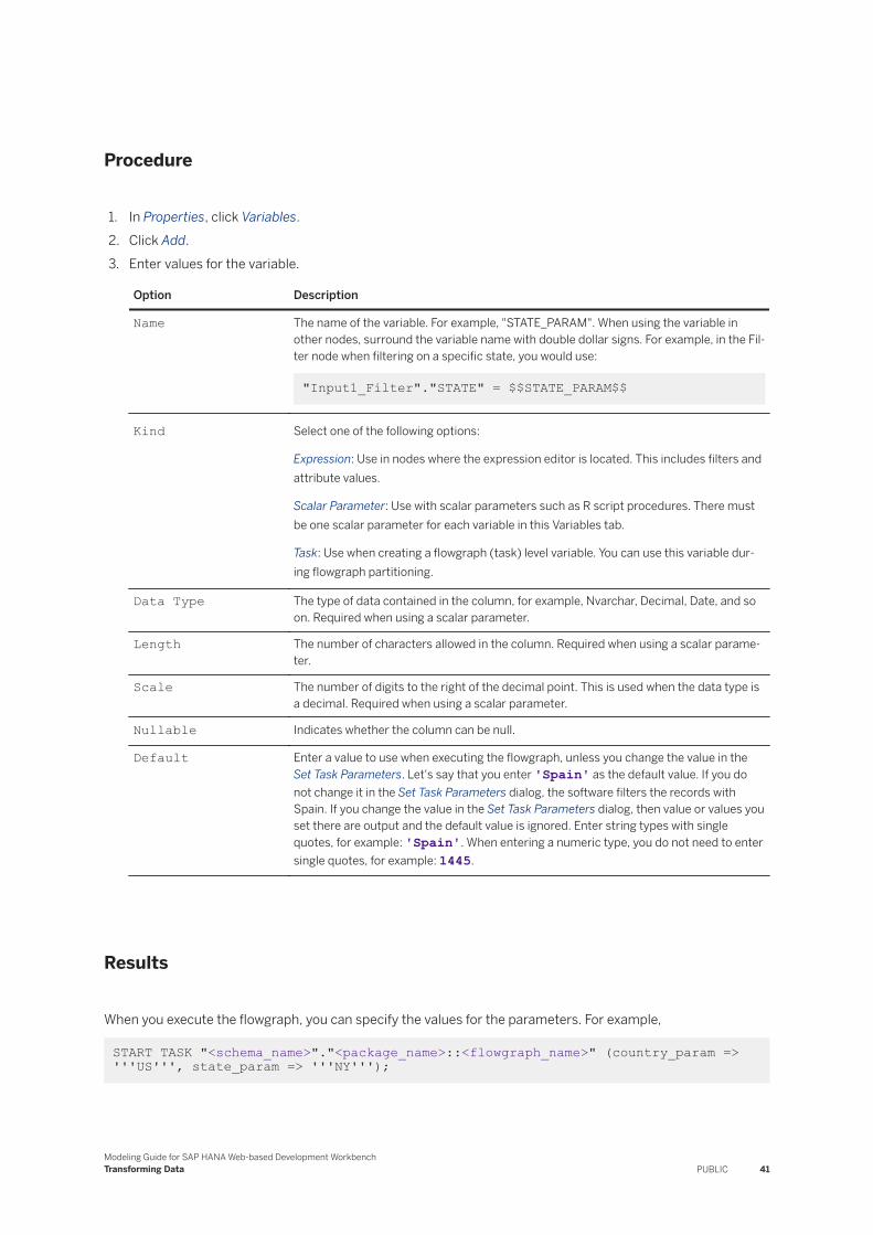
Procedure
1. In Properties, click Variables.2. Click Add.3. Enter values for the variable.
Option Description
Name The name of the variable. For example, "STATE_PARAM". When using the variable in other nodes, surround the variable name with double dollar signs. For example, in the Filter node when filtering on a specific state, you would use:
"Input1_Filter"."STATE" = $$STATE_PARAM$$
Kind Select one of the following options:
Expression: Use in nodes where the expression editor is located. This includes filters and attribute values.
Scalar Parameter: Use with scalar parameters such as R script procedures. There must be one scalar parameter for each variable in this Variables tab.
Task: Use when creating a flowgraph (task) level variable. You can use this variable during flowgraph partitioning.
Data Type The type of data contained in the column, for example, Nvarchar, Decimal, Date, and so on. Required when using a scalar parameter.
Length The number of characters allowed in the column. Required when using a scalar parameter.
Scale The number of digits to the right of the decimal point. This is used when the data type is a decimal. Required when using a scalar parameter.
Nullable Indicates whether the column can be null.
Default Enter a value to use when executing the flowgraph, unless you change the value in the Set Task Parameters. Let's say that you enter 'Spain' as the default value. If you do not change it in the Set Task Parameters dialog, the software filters the records with Spain. If you change the value in the Set Task Parameters dialog, then value or values you set there are output and the default value is ignored. Enter string types with single quotes, for example: 'Spain'. When entering a numeric type, you do not need to enter single quotes, for example: 1445.
Results
When you execute the flowgraph, you can specify the values for the parameters. For example,
START TASK "<schema_name>"."<package_name>::<flowgraph_name>" (country_param => '''US''', state_param => '''NY''');
Modeling Guide for SAP HANA Web-based Development WorkbenchTransforming Data PUBLIC 41
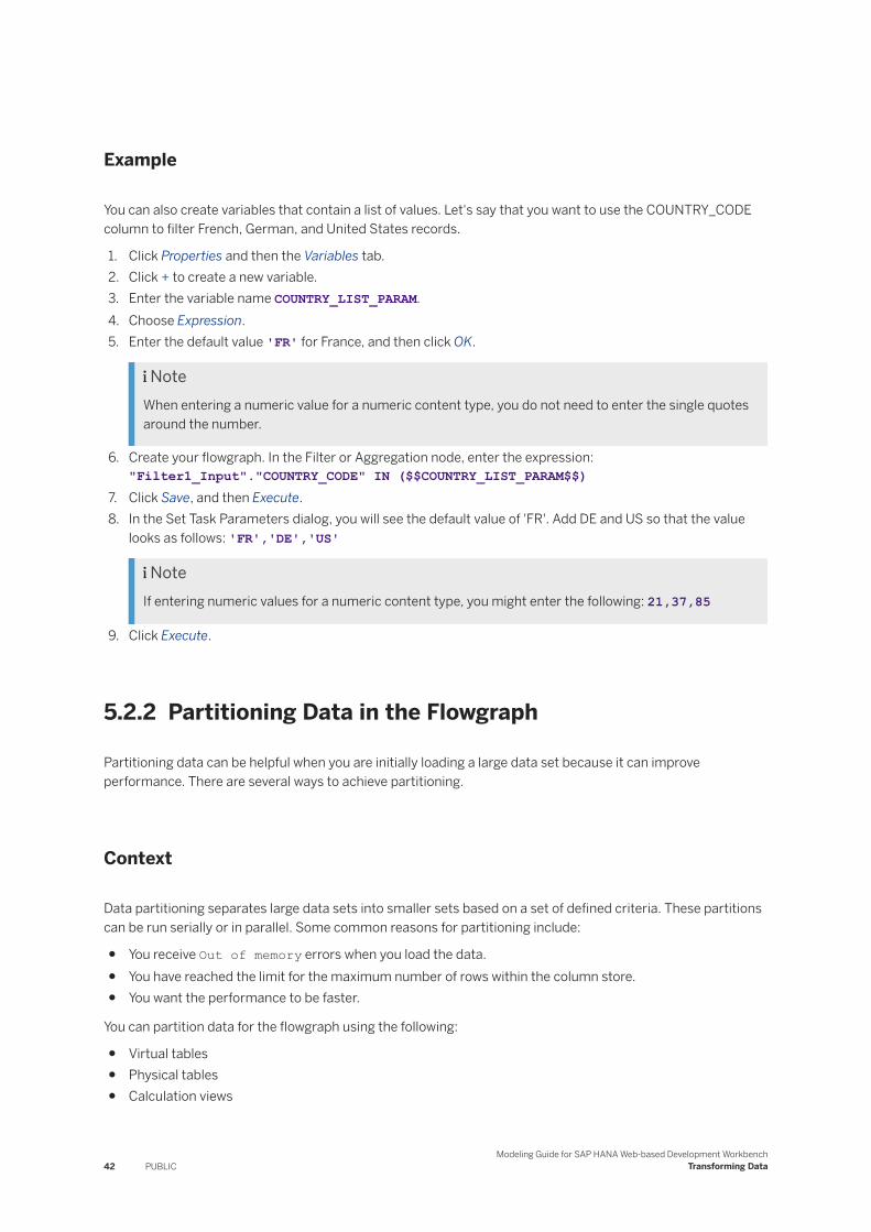
Example
You can also create variables that contain a list of values. Let's say that you want to use the COUNTRY_CODE column to filter French, German, and United States records.
1. Click Properties and then the Variables tab.2. Click + to create a new variable.3. Enter the variable name COUNTRY_LIST_PARAM.4. Choose Expression.5. Enter the default value 'FR' for France, and then click OK.
NoteWhen entering a numeric value for a numeric content type, you do not need to enter the single quotes around the number.
6. Create your flowgraph. In the Filter or Aggregation node, enter the expression: "Filter1_Input"."COUNTRY_CODE" IN ($$COUNTRY_LIST_PARAM$$)
7. Click Save, and then Execute.8. In the Set Task Parameters dialog, you will see the default value of 'FR'. Add DE and US so that the value
looks as follows: 'FR','DE','US'
NoteIf entering numeric values for a numeric content type, you might enter the following: 21,37,85
9. Click Execute.
5.2.2 Partitioning Data in the Flowgraph
Partitioning data can be helpful when you are initially loading a large data set because it can improve performance. There are several ways to achieve partitioning.
Context
Data partitioning separates large data sets into smaller sets based on a set of defined criteria. These partitions can be run serially or in parallel. Some common reasons for partitioning include:
● You receive Out of memory errors when you load the data.● You have reached the limit for the maximum number of rows within the column store.● You want the performance to be faster.
You can partition data for the flowgraph using the following:
● Virtual tables● Physical tables● Calculation views
42 PUBLICModeling Guide for SAP HANA Web-based Development Workbench
Transforming Data

● SQL views
You can partition data in two areas: at the task (flowgraph) level and at the Data Source node level. Partitioning at the task level is useful when your input data has several million rows or more. Currently, SAP HANA has a limitation where you cannot process more than two billion rows. Partitioning your data at the task level will likely reduce the load to less than two billion rows per partition. Typically, you see the benefit of using task level partitioning only with extremely large data sets. You can set the number of parallel partitions that are processed simultaneously. The transformation and loading to the target is done per partition. When you partition at the task level, you must select one data source in the flowgraph.
At the task level, you have several options for partitioning the data.
Task Partitioning Options Description
Automatic The application chooses the columns or you select some columns to use for partitioning. The result can be single-level or multi-level partitioning.
Manual: Single-level Choose the columns you want to use and whether to perform list, range, custom range, or column partitioning. The result is single-level partitioning.
Manual: Multi-level Advanced users can choose the columns and the type of partitioning and can create partitions within partitions.
If you have a small input data set, then using the partitioning options in the Data Source node might be better. There are some limitations however:
● Partitioning can be done only on virtual tables.● Only the input data is partitioned.● All of the partitions run in parallel; you cannot change the number of parallel partitions.
If you partition data in both the Data Source node and at the task level, the task-level partition settings take precedence and the specified Data Source node settings are ignored. If you have multiple Data Source nodes defined with partitioning, only the data source selected in the task partitioning is impacted during run time. All other Data Source nodes that are partitioned within the task are processed with their individual partitioning settings.
Partitioning can have an impact on your data results. When you partition at the task level, you must select one data source in the flowgraph. Because you can have multiple data sources within a flowgraph and only one can be partitioned at the task level, there may be slower performance when using a Join node or different data results when using the Match node.
NoteThe Match node may not be available to you depending on your application version or license agreement.
When using the Join node, one data source is partitioned and the other Data Source nodes are used in their entirety. If those sources have a significant amount of data, the Join node may act as a bottleneck because it has to wait for the other Data Source node data to load before being able to join the content with the task level partitioned data source.
Regarding the Match node results, the Match node finds duplicates only from within a single partition of data. However, if the partitioning is set on data that makes good break keys, then the Match node results are not an issue.
Modeling Guide for SAP HANA Web-based Development WorkbenchTransforming Data PUBLIC 43

Related Information
Manually Select Columns for Partitioning [page 44]Multi-level Partitioning [page 48]Supported Partitioning Data Types [page 49]
5.2.2.1 Manually Select Columns for Partitioning
Choose the columns and the type of partitioning you want to use to partition your data.
Context
When you are certain of the columns you want to use for partitioning, manually select columns and then and choose whether to perform list, range, or column partitioning. This topic describes single-level partitioning.
Procedure
1. Click the Properties icon. 2. In the Settings tab, set the Run-time Behavior Type to Batch Task or Real-time Task.3. (Optional) In the Variables tab, define any task variables that you want to use in the flowgraph. See Add a
Variable to the Flowgraph.4. Choose Extract, Transform & Load.5. In the Input Source list, view the supported data sources in your flowgraph. You can set partitions for one of
these sources only. Typically, this is the source with the largest set of data.6. In the Column option, choose the column that you want to use as the base of your partitioning. Set your
partitions based on the data in this column. If you use the Column partition type, then you do not need to set this option.
7. Set the Number of Parallel Partitions. For example, if you have five partitions, and you set the number of parallel partitions to 2, then partitions 1 and 2 run together. If partition 2 completes before partition 1, then partition 3 starts running, and so on. In general, the more partitions that you run in parallel, the faster the data is loaded. However, if there are memory issues, then data may not load because there are too many parallel partitions set. When this option is set to 1, partitioning runs in a series beginning with the first partition. When that partition finishes, the second partition starts, and so on.
You can set this option with a number or a variable. If you have defined a task variable in the Variables tab, you can enter it here with two dollar signs surrounding it, for example, $$variable_name$$. Use a task variable with a positive integer value only. To add task variables, see Add a Variable to the Flowgraph.
8. Select the Partition Type that you want to use.
44 PUBLICModeling Guide for SAP HANA Web-based Development Workbench
Transforming Data
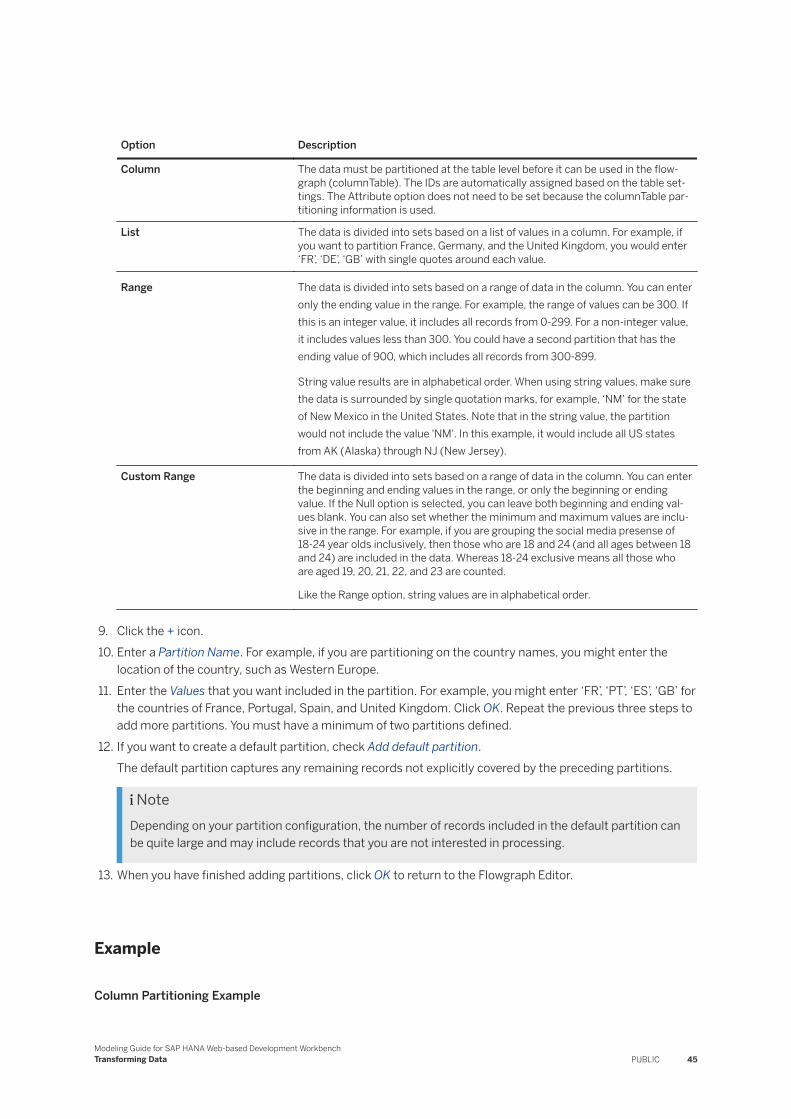
Option Description
Column The data must be partitioned at the table level before it can be used in the flow-graph (columnTable). The IDs are automatically assigned based on the table settings. The Attribute option does not need to be set because the columnTable partitioning information is used.
List The data is divided into sets based on a list of values in a column. For example, if you want to partition France, Germany, and the United Kingdom, you would enter ‘FR’, ‘DE’, ‘GB’ with single quotes around each value.
Range The data is divided into sets based on a range of data in the column. You can enter only the ending value in the range. For example, the range of values can be 300. If this is an integer value, it includes all records from 0-299. For a non-integer value, it includes values less than 300. You could have a second partition that has the ending value of 900, which includes all records from 300-899.
String value results are in alphabetical order. When using string values, make sure the data is surrounded by single quotation marks, for example, ‘NM’ for the state of New Mexico in the United States. Note that in the string value, the partition would not include the value 'NM'. In this example, it would include all US states from AK (Alaska) through NJ (New Jersey).
Custom Range The data is divided into sets based on a range of data in the column. You can enter the beginning and ending values in the range, or only the beginning or ending value. If the Null option is selected, you can leave both beginning and ending values blank. You can also set whether the minimum and maximum values are inclusive in the range. For example, if you are grouping the social media presense of 18-24 year olds inclusively, then those who are 18 and 24 (and all ages between 18 and 24) are included in the data. Whereas 18-24 exclusive means all those who are aged 19, 20, 21, 22, and 23 are counted.
Like the Range option, string values are in alphabetical order.
9. Click the + icon.10. Enter a Partition Name. For example, if you are partitioning on the country names, you might enter the
location of the country, such as Western Europe.11. Enter the Values that you want included in the partition. For example, you might enter ‘FR’, ‘PT’, ‘ES’, ‘GB’ for
the countries of France, Portugal, Spain, and United Kingdom. Click OK. Repeat the previous three steps to add more partitions. You must have a minimum of two partitions defined.
12. If you want to create a default partition, check Add default partition.The default partition captures any remaining records not explicitly covered by the preceding partitions.
NoteDepending on your partition configuration, the number of records included in the default partition can be quite large and may include records that you are not interested in processing.
13. When you have finished adding partitions, click OK to return to the Flowgraph Editor.
Example
Column Partitioning Example
Modeling Guide for SAP HANA Web-based Development WorkbenchTransforming Data PUBLIC 45
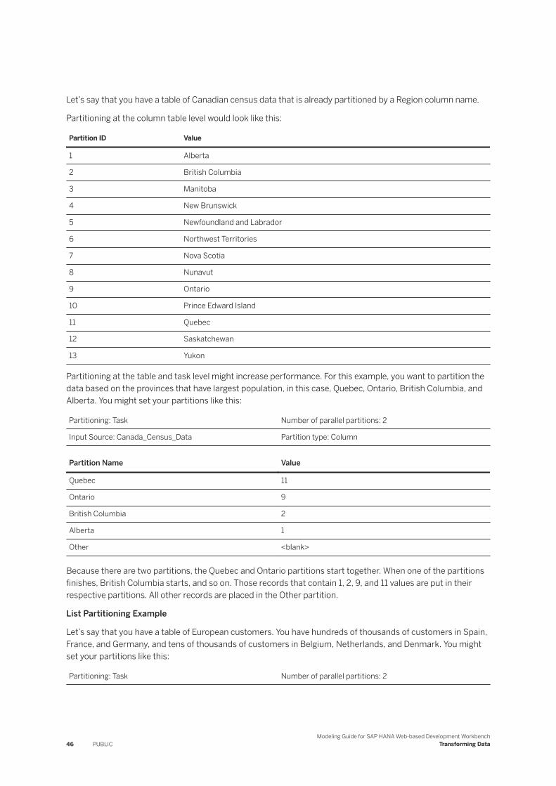
Let’s say that you have a table of Canadian census data that is already partitioned by a Region column name.
Partitioning at the column table level would look like this:
Partition ID Value
1 Alberta
2 British Columbia
3 Manitoba
4 New Brunswick
5 Newfoundland and Labrador
6 Northwest Territories
7 Nova Scotia
8 Nunavut
9 Ontario
10 Prince Edward Island
11 Quebec
12 Saskatchewan
13 Yukon
Partitioning at the table and task level might increase performance. For this example, you want to partition the data based on the provinces that have largest population, in this case, Quebec, Ontario, British Columbia, and Alberta. You might set your partitions like this:
Partitioning: Task Number of parallel partitions: 2
Input Source: Canada_Census_Data Partition type: Column
Partition Name Value
Quebec 11
Ontario 9
British Columbia 2
Alberta 1
Other <blank>
Because there are two partitions, the Quebec and Ontario partitions start together. When one of the partitions finishes, British Columbia starts, and so on. Those records that contain 1, 2, 9, and 11 values are put in their respective partitions. All other records are placed in the Other partition.
List Partitioning Example
Let’s say that you have a table of European customers. You have hundreds of thousands of customers in Spain, France, and Germany, and tens of thousands of customers in Belgium, Netherlands, and Denmark. You might set your partitions like this:
Partitioning: Task Number of parallel partitions: 2
46 PUBLICModeling Guide for SAP HANA Web-based Development Workbench
Transforming Data
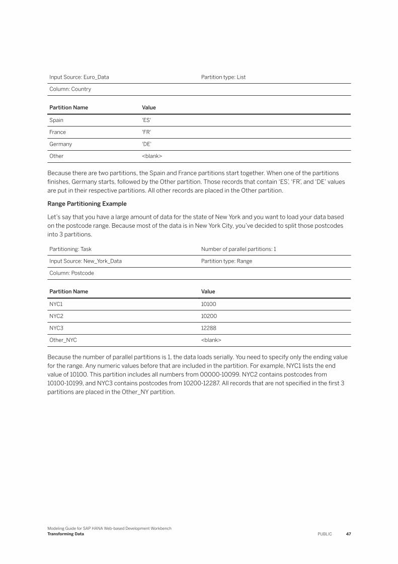
Input Source: Euro_Data Partition type: List
Column: Country
Partition Name Value
Spain 'ES'
France 'FR'
Germany 'DE'
Other <blank>
Because there are two partitions, the Spain and France partitions start together. When one of the partitions finishes, Germany starts, followed by the Other partition. Those records that contain ‘ES’, ‘FR’, and ‘DE’ values are put in their respective partitions. All other records are placed in the Other partition.
Range Partitioning Example
Let’s say that you have a large amount of data for the state of New York and you want to load your data based on the postcode range. Because most of the data is in New York City, you’ve decided to split those postcodes into 3 partitions.
Partitioning: Task Number of parallel partitions: 1
Input Source: New_York_Data Partition type: Range
Column: Postcode
Partition Name Value
NYC1 10100
NYC2 10200
NYC3 12288
Other_NYC <blank>
Because the number of parallel partitions is 1, the data loads serially. You need to specify only the ending value for the range. Any numeric values before that are included in the partition. For example, NYC1 lists the end value of 10100. This partition includes all numbers from 00000-10099. NYC2 contains postcodes from 10100-10199, and NYC3 contains postcodes from 10200-12287. All records that are not specified in the first 3 partitions are placed in the Other_NY partition.
Modeling Guide for SAP HANA Web-based Development WorkbenchTransforming Data PUBLIC 47
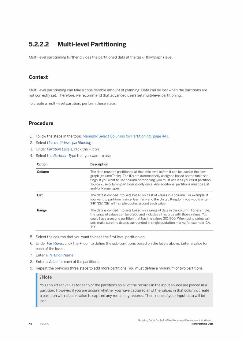
5.2.2.2 Multi-level Partitioning
Multi-level partitioning further divides the partitioned data at the task (flowgraph) level.
Context
Multi-level partitioning can take a considerable amount of planning. Data can be lost when the partitions are not correctly set. Therefore, we recommend that advanced users set multi-level partitioning.
To create a multi-level partition, perform these steps:
Procedure
1. Follow the steps in the topic Manually Select Columns for Partitioning [page 44].2. Select Use multi-level partitioning.3. Under Partition Levels, click the + icon.4. Select the Partition Type that you want to use.
Option Description
Column The data must be partitioned at the table level before it can be used in the flow-graph (columnTable). The IDs are automatically assigned based on the table settings. If you want to use column partitioning, you must use it as your first partition. You can use column partitioning only once. Any additional partitions must be List and/or Range types.
List The data is divided into sets based on a list of values in a column. For example, if you want to partition France, Germany and the United Kingdom, you would enter ‘FR’, ‘DE’, ‘GB’ with single quotes around each value.
Range The data is divided into sets based on a range of data in the column. For example, the range of values can be 0,300 and includes all records with those values. You could have a second partition that has the values 301,900. When using string values, make sure the data is surrounded in single quotation marks, for example ‘CA’, ‘NY’.
5. Select the column that you want to base the first level partition on.6. Under Partitions, click the + icon to define the sub-partitions based on the levels above. Enter a value for
each of the levels.7. Enter a Partition Name.8. Enter a Value for each of the partitions.9. Repeat the previous three steps to add more partitions. You must define a minimum of two partitions.
NoteYou should set values for each of the partitions so all of the records in the input source are placed in a partition. However, if you are unsure whether you have captured all of the values in that column, create a partition with a blank value to capture any remaining records. Then, none of your input data will be lost.
48 PUBLICModeling Guide for SAP HANA Web-based Development Workbench
Transforming Data
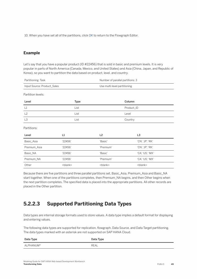
10. When you have set all of the partitions, click OK to return to the Flowgraph Editor.
Example
Let’s say that you have a popular product (ID #22456) that is sold in basic and premium levels. It is very popular in parts of North America (Canada, Mexico, and United States) and Asia (China, Japan, and Republic of Korea), so you want to partition the data based on product, level, and country.
Partitioning: Task Number of parallel partitions: 3
Input Source: Product_Sales Use multi-level partitioning
Partition levels:
Level Type Column
L1 List Product_ID
L2 List Level
L3 List Country
Partitions:
Level L1 L2 L3
Basic_Asia ‘22456’ ‘Basic’ ‘CN’, ‘JP’, ‘RK’
Premium_Asia ‘22456’ ‘Premium’ ‘CN’, ‘JP’, ‘RK’
Basic_NA ‘22456’ ‘Basic’ ‘CA’, ‘US’, ‘MX’
Premium_NA ‘22456’ ‘Premium’ ‘CA’, ‘US’, ‘MX’
Other <blank> <blank> <blank>
Because there are five partitions and three parallel partitions set, Basic_Asia, Premium_Asia and Basic_NA start together. When one of the partitions completes, then Premium_NA begins, and then Other begins when the next partition completes. The specified data is placed into the appropriate partitions. All other records are placed in the Other partition.
5.2.2.3 Supported Partitioning Data Types
Data types are internal storage formats used to store values. A data type implies a default format for displaying and entering values.
The following data types are supported for replication, flowgraph, Data Source, and Data Target partitioning. The data types marked with an asterisk are not supported on SAP HANA Cloud.
Data Type Data Type
ALPHANUM* REAL
Modeling Guide for SAP HANA Web-based Development WorkbenchTransforming Data PUBLIC 49
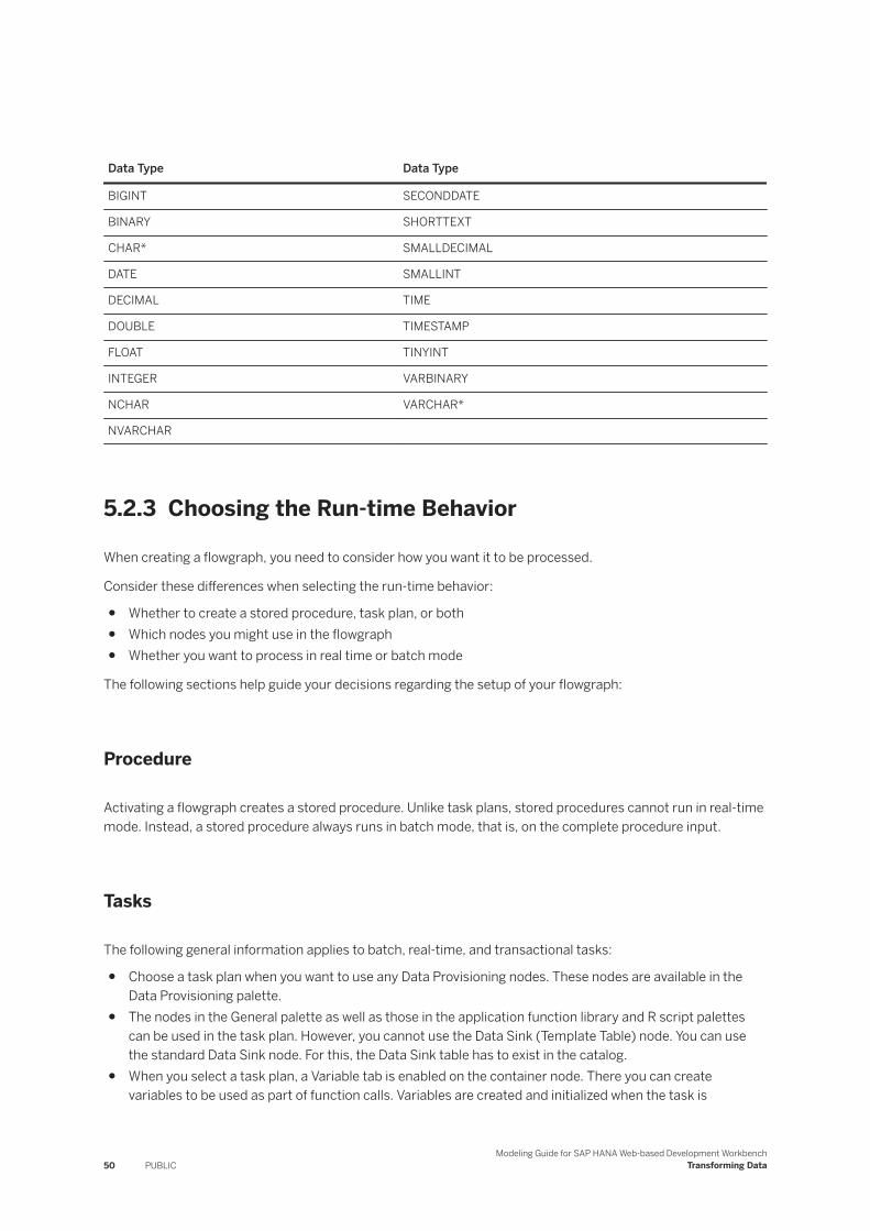
Data Type Data Type
BIGINT SECONDDATE
BINARY SHORTTEXT
CHAR* SMALLDECIMAL
DATE SMALLINT
DECIMAL TIME
DOUBLE TIMESTAMP
FLOAT TINYINT
INTEGER VARBINARY
NCHAR VARCHAR*
NVARCHAR
5.2.3 Choosing the Run-time Behavior
When creating a flowgraph, you need to consider how you want it to be processed.
Consider these differences when selecting the run-time behavior:
● Whether to create a stored procedure, task plan, or both● Which nodes you might use in the flowgraph● Whether you want to process in real time or batch mode
The following sections help guide your decisions regarding the setup of your flowgraph:
Procedure
Activating a flowgraph creates a stored procedure. Unlike task plans, stored procedures cannot run in real-time mode. Instead, a stored procedure always runs in batch mode, that is, on the complete procedure input.
Tasks
The following general information applies to batch, real-time, and transactional tasks:
● Choose a task plan when you want to use any Data Provisioning nodes. These nodes are available in the Data Provisioning palette.
● The nodes in the General palette as well as those in the application function library and R script palettes can be used in the task plan. However, you cannot use the Data Sink (Template Table) node. You can use the standard Data Sink node. For this, the Data Sink table has to exist in the catalog.
● When you select a task plan, a Variable tab is enabled on the container node. There you can create variables to be used as part of function calls. Variables are created and initialized when the task is
50 PUBLICModeling Guide for SAP HANA Web-based Development Workbench
Transforming Data
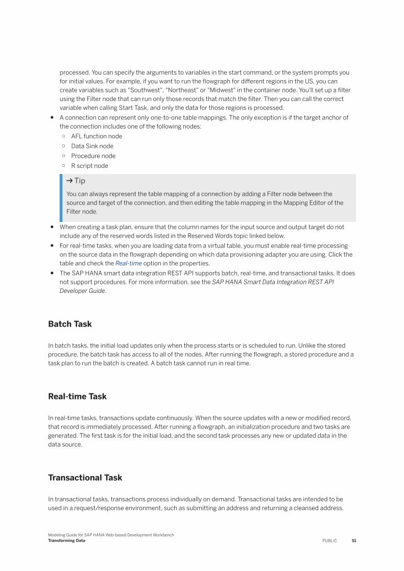
processed. You can specify the arguments to variables in the start command, or the system prompts you for initial values. For example, if you want to run the flowgraph for different regions in the US, you can create variables such as "Southwest", "Northeast" or "Midwest" in the container node. You'll set up a filter using the Filter node that can run only those records that match the filter. Then you can call the correct variable when calling Start Task, and only the data for those regions is processed.
● A connection can represent only one-to-one table mappings. The only exception is if the target anchor of the connection includes one of the following nodes:○ AFL function node○ Data Sink node○ Procedure node○ R script node
TipYou can always represent the table mapping of a connection by adding a Filter node between the source and target of the connection, and then editing the table mapping in the Mapping Editor of the Filter node.
● When creating a task plan, ensure that the column names for the input source and output target do not include any of the reserved words listed in the Reserved Words topic linked below.
● For real-time tasks, when you are loading data from a virtual table, you must enable real-time processing on the source data in the flowgraph depending on which data provisioning adapter you are using. Click the table and check the Real-time option in the properties.
● The SAP HANA smart data integration REST API supports batch, real-time, and transactional tasks. It does not support procedures. For more information, see the SAP HANA Smart Data Integration REST API Developer Guide.
Batch Task
In batch tasks, the initial load updates only when the process starts or is scheduled to run. Unlike the stored procedure, the batch task has access to all of the nodes. After running the flowgraph, a stored procedure and a task plan to run the batch is created. A batch task cannot run in real time.
Real-time Task
In real-time tasks, transactions update continuously. When the source updates with a new or modified record, that record is immediately processed. After running a flowgraph, an initialization procedure and two tasks are generated. The first task is for the initial load, and the second task processes any new or updated data in the data source.
Transactional Task
In transactional tasks, transactions process individually on demand. Transactional tasks are intended to be used in a request/response environment, such as submitting an address and returning a cleansed address.
Modeling Guide for SAP HANA Web-based Development WorkbenchTransforming Data PUBLIC 51
Unlike the real-time task, only a single task generates to process any new or updated data in the data source. You cannot use a virtual table for transactional tasks. Use Table-Type as the input source.
Related Information
Reserved Words [page 54]Add a Variable to the FlowgraphSave and Execute a Flowgraph [page 215]Administration Guide for SAP HANA smart data integration and SAP HANA Smart Data Quality (HTML)
5.2.4 Importing an Agile Data Preparation Flowgraph
Import and configure a flowgraph originally created in SAP Agile Data Preparation.
Context
After you've configured a small set of data in SAP Agile Data Preparation (ADP), you can import what was called a worksheet, now called a flowgraph, into SAP HANA Web-based Development Workbench to process a larger set of data. Because ADP and Web-based Development Workbench do not utilize identical technology, there are some processing differences. You can import and process the flowgraph, but the output will be different because the Web-based Development Workbench automatically outputs duplicate records. You can follow the steps at the bottom of this topic to make the output similar to that of ADP.
Export the worksheet from ADP and import it as a flowgraph into Web-based Development Workbench.
Procedure
1. In ADP, after configuring the worksheet, click Action History, and then click the download icon.
The worksheet is saved to your downloads area.2. In Web-based Development Workbench, right-click on the package name in the catalog panel. Choose
Import File .3. Browse to the location where the worksheet was exported from ADP. Click Import and then click the x to
close the window.4. Right-click on the package name, and then choose Refresh.5. If you see an error, open the Template Table node, which is the last node in the flowgraph. In the Authoring
Schema option, select the correct schema, and click Back to return to the flowgraph.
52 PUBLICModeling Guide for SAP HANA Web-based Development Workbench
Transforming Data
Next Steps
Now that the flowgraph is open, let's show the differences. Notice that the Input Type area has a node called OUTPUT. This label means that the source was output from ADP. Rest assured that this is a representation of the source table. When you execute the flowgraph, you will be asked to select an input source.
Another difference you may notice is that there isn't a Best Record node. ADP has this technology, but it is not implemented in Web-based Development Workbench.
Before running the flowgraph, there are a few things to do so the output in Web-based Development Workbench provides the same results as in ADP.
1. Add a Filter node to the flowgraph. Disconnect the pipe between the Union node and the Writer. Connect the pipe from the Union node to the Filter node.
2. Double-click to open the Filter node. You may notice many output columns that begin with MATCH_ that were not shown in the ADP worksheet. You can manually delete each one of these, if you want to reduce the number of columns, but this is not required. Click the Filter Node tab. Enter the following expression into the Filter node so that only unique and master records are output.
Sample Code
("Filter1_Input"."GROUP_ID_1" is null) OR ("Filter1_Input"."GROUP_ID_1" is not null and "Filter1_Input"."GROUP_MASTER_1" = 'M')
3. Connect the output from the Filter node to the Writer node.4. (Optional) Open the Writer node. The output name is automatically generated. You might want to change
the name to something more understandable in the Node Name option.5. Click Save and then Execute. You are prompted to select an input source. Select the table and then click OK
to run the flowgraph.
Best Practices
● Do not delete the Input Type node, which is labeled OUTPUT. This invalidates the flowgraph, and you will have to start over.
● With the exception of the Filter node, do not add or delete any nodes, especially before the Cleanse and Match nodes.
● You can change some options and settings within the nodes. However, the output will no longer match what was output in ADP.
● You cannot export a flowgraph from Web-based Development Workbench and open it in ADP.
Related Information
Filter [page 166]CleanseMatch [page 187]Save and Execute a Flowgraph [page 215]
Modeling Guide for SAP HANA Web-based Development WorkbenchTransforming Data PUBLIC 53
5.2.5 Use the Expression Editor
The Expression Editor is available in the Aggregation, Case, Join, Lookup, Map Operation, Projection, and Table Comparison nodes.
The Expression Editor is available in the Filter tab, Having tab, Mapping, and others. An expression is either a mathematical calculation, for example obtaining the sum of column1 and column5, or a way of selecting data that meets the criteria of a value, for example the product is less than $50.
To use the Expression Editor, perform these steps:
1. Click the Filters tab to view the columns and the available functions.2. Select the columns to use in your expression. You can drag and drop column names from the list and place
them in the text box above.3. Select one of the available functions from the categories in the Functions pane. See the SAP HANA SQL and
System Views Reference for more information about each function.4. Click or type any operators to complete the expression.
Related Information
Alphabetical List of Functions (SAP HANA SQL and System Views Reference)
5.2.6 Reserved Words
The following words have special meaning for Data Provisioning nodes.
Therefore, these words should not be used as column names or attribute names in your input source or output target when you choose to create a task plan flowgraph or a replication task. They are reserved with any combination of upper- and lower-case letters.
● _BEFORE_*● _COMMIT_TIMESTAMP● _OP_CODE
5.2.7 Nodes Available for Real-time Processing
A list showing which nodes can be used in a real-time enabled flowgraph.
Node Available for real-time processing
Application Function Library (AFL) No
Aggregation Yes
54 PUBLICModeling Guide for SAP HANA Web-based Development Workbench
Transforming Data

Node Available for real-time processing
Case Yes
Cleanse Yes
Data Mask Yes
Date Generation No
Filter Yes
Geocode Yes
Hierarchical No
History Preserving Yes
Join No
Lookup Yes
Map Operation Yes
Match No
Pivot No
Procedure No
R-Script No
Row Generation No
Sort Yes
Table Comparison Yes
Union Yes
Unpivot No
5.3 Transforming Data Using SAP HANA Web-based Development Workbench
Use the flowgraph editor in SAP HANA Web-based Development Workbench to create flowgraphs to transform and virtualize data.
Use this tool to develop applications in a Web browser without having to install any development tools. This is a quick alternative to using SAP HANA studio's application function modeler.
In SAP HANA Web-based Development Workbench, the data flows are stored as flowgraph objects with an extension of .hdbflowgraph. When activated, the data flows generate a stored procedure. They can consume:
● database tables, views, and links to external resources● relational operators such as filter, join, and union● custom procedures written in SQL script● functions from optional components such as the Application Function Library (AFL) or Business Function
Library (BFL)
Modeling Guide for SAP HANA Web-based Development WorkbenchTransforming Data PUBLIC 55
As your data moves from its source to its target, it passes through a sequence of one or more transforms. You can map input to output columns in the node settings. Columns that you do not map as inputs to a replication task or flowgraph will not be sent over the network to be processed by SAP HANA. Excluding columns as inputs can improve performance, for example if they contain large object types. You can also choose to enhance security by excluding columns that, for example, include sensitive data such as passwords.
See the SAP HANA Developer Guide for SAP HANA Web Workbench for more information about SAP HANA Web-based Development Workbench.
NoteSAP HANA smart data integration and SAP HANA smart data quality add much more functionality to flowgraph design, such as data cleansing, geocoding, masking, date and row generation, and so on, as well as many capabilities outside of flowgraphs. For information about the capabilities available for your license and installation scenario, refer to the Feature Scope Description (FSD) for your specific SAP HANA version on the SAP HANA Platform page.
Parent topic: Transforming Data [page 38]
Previous: Defining Flowgraph Behavior [page 39]
Next task: Save and Execute a Flowgraph [page 215]
Related Information
Configure the Flowgraph in SAP HANA Web-based Development Workbench [page 57]Configure Nodes in SAP HANA Web-based Development Workbench [page 58]AFL Function [page 59]Aggregation [page 60]Case [page 61]Cleanse [page 63]Data Mask [page 131]Data Sink [page 155]Data Source [page 159]Date Generator [page 165]Filter [page 166]Geocode [page 167]Hierarchical [page 179]History Preserving [page 181]Input Type [page 183]Join [page 184]Lookup [page 185]Map Operation [page 186]Match [page 187]
56 PUBLICModeling Guide for SAP HANA Web-based Development Workbench
Transforming Data
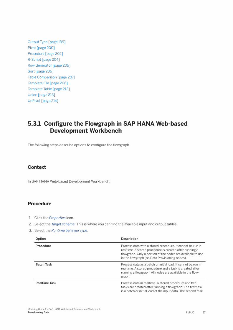
Output Type [page 199]Pivot [page 200]Procedure [page 202]R-Script [page 204]Row Generator [page 205]Sort [page 206]Table Comparison [page 207]Template File [page 208]Template Table [page 212]Union [page 213]UnPivot [page 214]
5.3.1 Configure the Flowgraph in SAP HANA Web-based Development Workbench
The following steps describe options to configure the flowgraph.
Context
In SAP HANA Web-based Development Workbench:
Procedure
1. Click the Properties icon.2. Select the Target schema. This is where you can find the available input and output tables.3. Select the Runtime behavior type.
Option Description
Procedure Process data with a stored procedure. It cannot be run in realtime. A stored procedure is created after running a flowgraph. Only a portion of the nodes are available to use in the flowgraph (no Data Provisioning nodes).
Batch Task Process data as a batch or initial load. It cannot be run in realtime. A stored procedure and a task is created after running a flowgraph. All nodes are available in the flow-graph.
Realtime Task Process data in realtime. A stored procedure and two tasks are created after running a flowgraph. The first task is a batch or initial load of the input data. The second task
Modeling Guide for SAP HANA Web-based Development WorkbenchTransforming Data PUBLIC 57
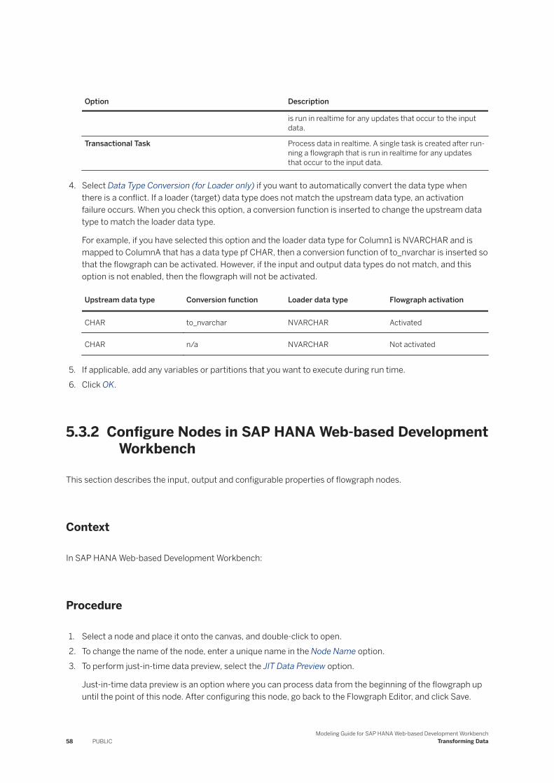
Option Description
is run in realtime for any updates that occur to the input data.
Transactional Task Process data in realtime. A single task is created after running a flowgraph that is run in realtime for any updates that occur to the input data.
4. Select Data Type Conversion (for Loader only) if you want to automatically convert the data type when there is a conflict. If a loader (target) data type does not match the upstream data type, an activation failure occurs. When you check this option, a conversion function is inserted to change the upstream data type to match the loader data type.
For example, if you have selected this option and the loader data type for Column1 is NVARCHAR and is mapped to ColumnA that has a data type pf CHAR, then a conversion function of to_nvarchar is inserted so that the flowgraph can be activated. However, if the input and output data types do not match, and this option is not enabled, then the flowgraph will not be activated.
Upstream data type Conversion function Loader data type Flowgraph activation
CHAR to_nvarchar NVARCHAR Activated
CHAR n/a NVARCHAR Not activated
5. If applicable, add any variables or partitions that you want to execute during run time.6. Click OK.
5.3.2 Configure Nodes in SAP HANA Web-based Development Workbench
This section describes the input, output and configurable properties of flowgraph nodes.
Context
In SAP HANA Web-based Development Workbench:
Procedure
1. Select a node and place it onto the canvas, and double-click to open.2. To change the name of the node, enter a unique name in the Node Name option.3. To perform just-in-time data preview, select the JIT Data Preview option.
Just-in-time data preview is an option where you can process data from the beginning of the flowgraph up until the point of this node. After configuring this node, go back to the Flowgraph Editor, and click Save.
58 PUBLICModeling Guide for SAP HANA Web-based Development Workbench
Transforming Data
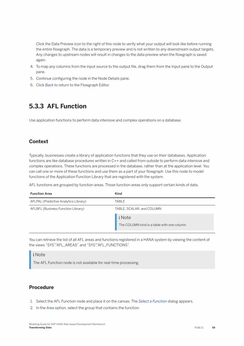
Click the Data Preview icon to the right of this node to verify what your output will look like before running the entire flowgraph. The data is a temporary preview and is not written to any downstream output targets. Any changes to upstream nodes will result in changes to the data preview when the flowgraph is saved again.
4. To map any columns from the input source to the output file, drag them from the Input pane to the Output pane.
5. Continue configuring the node in the Node Details pane.6. Click Back to return to the Flowgraph Editor.
5.3.3 AFL Function
Use application functions to perform data intensive and complex operations on a database.
Context
Typically, businesses create a library of application functions that they use on their databases. Application functions are like database procedures written in C++ and called from outside to perform data intensive and complex operations. These functions are processed in the database, rather than at the application level. You can call one or more of these functions and use them as a part of your flowgraph. Use this node to model functions of the Application Function Library that are registered with the system.
AFL functions are grouped by function areas. Those function areas only support certain kinds of data.
Function Area Kind
AFLPAL (Predictive Analytics Library) TABLE
AFLBFL (Business Function Library) TABLE, SCALAR, and COLUMN
NoteThe COLUMN kind is a table with one column.
You can retrieve the list of all AFL areas and functions registered in a HANA system by viewing the content of the views “SYS”.”AFL_AREAS” and “SYS”.”AFL_FUNCTIONS”.
NoteThe AFL Function node is not available for real-time processing.
Procedure
1. Select the AFL Function node and place it on the canvas. The Select a Function dialog appears.2. In the Area option, select the group that contains the function.
Modeling Guide for SAP HANA Web-based Development WorkbenchTransforming Data PUBLIC 59
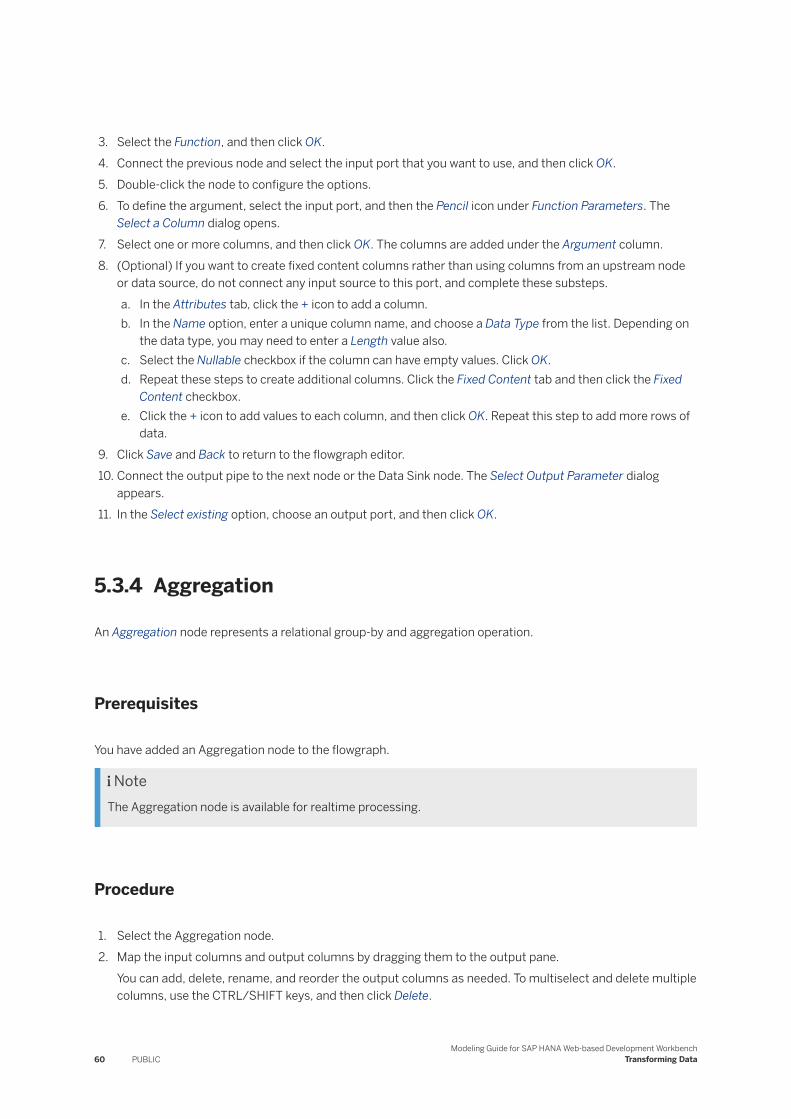
3. Select the Function, and then click OK.4. Connect the previous node and select the input port that you want to use, and then click OK.5. Double-click the node to configure the options.6. To define the argument, select the input port, and then the Pencil icon under Function Parameters. The
Select a Column dialog opens.7. Select one or more columns, and then click OK. The columns are added under the Argument column.8. (Optional) If you want to create fixed content columns rather than using columns from an upstream node
or data source, do not connect any input source to this port, and complete these substeps.a. In the Attributes tab, click the + icon to add a column.b. In the Name option, enter a unique column name, and choose a Data Type from the list. Depending on
the data type, you may need to enter a Length value also.c. Select the Nullable checkbox if the column can have empty values. Click OK.d. Repeat these steps to create additional columns. Click the Fixed Content tab and then click the Fixed
Content checkbox.e. Click the + icon to add values to each column, and then click OK. Repeat this step to add more rows of
data.9. Click Save and Back to return to the flowgraph editor.10. Connect the output pipe to the next node or the Data Sink node. The Select Output Parameter dialog
appears.11. In the Select existing option, choose an output port, and then click OK.
5.3.4 Aggregation
An Aggregation node represents a relational group-by and aggregation operation.
Prerequisites
You have added an Aggregation node to the flowgraph.
NoteThe Aggregation node is available for realtime processing.
Procedure
1. Select the Aggregation node.2. Map the input columns and output columns by dragging them to the output pane.
You can add, delete, rename, and reorder the output columns as needed. To multiselect and delete multiple columns, use the CTRL/SHIFT keys, and then click Delete.
60 PUBLICModeling Guide for SAP HANA Web-based Development Workbench
Transforming Data
3. In the Aggregations tab, specify the columns that you want to have the aggregate or group-by actions taken upon. Drag the input fields and then select the action from the drop-down list.
4. (Optional) Select the Having tab to run a filter on an aggregation function. Enter the expression. To view the options in the expression editor, click Load Elements & Functions. You can drag and drop the input and output columns from the Elements pane, then drag an aggregation function from the Functions pane. Click or type the appropriate operators. For example, if you want to find the transactions that are over $75,000 based on the average sales in the 1st quarter, your expression might look like this: AVG("Aggregation1_Input"."SALES") > 75000.
Option Description
Avg Calculates the average of a given set of column values
Count Returns the number of values in a table column
Group-by Use for specifying a list of columns for which you want to combine output. For example, you might want to group sales orders by date to find the total sales ordered on a particular date.
Max Returns the maximum value from a list
Min Returns the minimum value from a list
Sum Calculates the sum of a given set of values
5. (Optional) Select the Filter Node tab to compare the column name against a constant value. Click Load Elements & Functions to populate the Expression Editor. Enter the expression by dragging the column names, the function, and entering the operators from the pane at the bottom of the node. For example, if you want to the number of sales that are greater than 10000, your expression might look like this: "Aggregation1_input"."SALES" > 10000. See the SAP HANA SQL and System Views Reference for more information about each function.
6. Click Save to return to the Flowgraph Editor.
Related Information
Using the Mapping Editor (SAP HANA Developer Guide)Alphabetical List of Functions (SAP HANA SQL and System Views Reference)
5.3.5 Case
Specifies multiple paths in a single node; the rows are separated and processed in different ways.
Context
Route input records from a single source to one or more output paths. You can simplify branch logic in data flows by consolidating case or decision-making logic in one node. Paths are defined in an expression table.
Modeling Guide for SAP HANA Web-based Development WorkbenchTransforming Data PUBLIC 61
NoteThe Case node is available for real-time processing.
Procedure
1. (Optional) Select JIT Data Preview to create a preview of the data as it would be output up to this point in the flowgraph. All transformations from previous nodes, including the changes set in this node are shown in the preview by clicking the Data Preview icon on the canvas next to this node.
2. In the Output pane, click + to add one or more case expressions.3. (Optional) In the General tab, select Produce default output to add a default output target, such as a table.
There can be one default output target only. If the record does not match any of the other output cases, it goes to the default output table.
4. (Optional) Select Row can be true for one case only to specify whether a row can be included in only one or many output targets. For example, you might have a partial address that does not include a country name such as 455 Rue de la Marine. It is possible that this row could be output to the tables named Canada_Customer, France_Customer, and Other_Customer. Select this option to output the record into the first output table whose expression returns TRUE. Not selecting this option would put the record in all three tables.
5. Click the Case Label Detail tab.6. Select the case from the Output pane. You can change the name. For example, you might have an
expression for "Marketing," "Finance," and "Development," and the default expression might be for "Others." The default expression is used when all other Case expressions evaluate to false.
7. Enter the expression for each of the cases.
Related Information
Use the Expression Editor [page 54]Alphabetical List of Functions (SAP HANA SQL and System Views Reference)
62 PUBLICModeling Guide for SAP HANA Web-based Development Workbench
Transforming Data
5.3.6 Cleanse
Identifies, parses, validates, and formats the following data: address, person name, organization name, occupational title, phone number, and email address.
Context
Address reference data comes in the form of country-specific directories. For information about downloading and deploying directories, see “Directories” in the Installation and Configuration Guide for SAP HANA Smart Data Integration and SAP HANA Smart Data Quality.
Only one input source is allowed.
NoteThe Cleanse node is available for real-time processing.
Procedure
1. Click the Cleanse node, place it on the canvas, and connect the source data or the previous node. The Cleanse Configuration window appears.
2. Select any additional columns to output. The default columns are automatically mapped based on the input data.
3. (Optional) Add or remove entire input categories by selecting or de-selecting the checkbox next to the component name, such as Person, Firm and Address.
NoteThe categories shown are based on the input data. You will only see those categories if your data contains that type of information. For example, if your input data does not contain email data, then the email component is not shown.
4. (Optional) To add or remove specific columns, click the pencil icon next to the category name. For example, if you want to remove Address2 and Address3 from the Address category, de-select those columns in the Edit Component window, and then click OK.
5. (Optional) To edit the content types, click Edit Defaults Edit Content Types . Review the column names and content types making changes as necessary by clicking the down arrow next to the content type and selecting a different content type. Click Apply.
6. (Optional) To change the format and settings for this flowgraph, click Edit Defaults Edit Settings . For more information about the options available on the Cleanse Settings window, see Change Default Cleanse Settings [page 64]
7. Click Next.8. Based on the input data provided, information is shown about the output columns either with sample data
or with the column names. Click the right and left arrows to make any final formatting changes and additions to the output columns. You can also make these changes on the Cleanse Settings window.
Modeling Guide for SAP HANA Web-based Development WorkbenchTransforming Data PUBLIC 63
NoteBased on the input data provided, information is shown about the output columns either with sample data or with the column names.. Click the right and left arrows to make any final formatting changes and additions to the output columns. You can also make these changes on the Cleanse Settings window.
9. Review the suggested actions. To implement the suggested action, click Apply and then OK for each action you want included.
10. (Optional) To include additional output fields such as address assignment levels or information codes, click Customize Manually. For each category, select the type of additional information that you want to add. Click the checkbox next to each output field, then click Apply.
11. Click Finish.12. On the flowgraph editor, select an output table. If you have enabled suggestion lists, select two output
tables. Select the output type for each table. "Output" is for valid, cleansed addresses. "Suggestion List" is for the list of possible valid addresses for those records that are invalid.
Related Information
Change Cleanse Settings [page 64]About Cleansing [page 69]About Suggestion Lists [page 96]Cleanse Input Columns [page 98]Cleanse Output Columns [page 102]
5.3.6.1 Change Cleanse Settings
Set the cleanse preferences.
Context
The Cleanse settings are used as a template for all future projects using the Cleanse node. These settings can be overridden for each project.
Procedure
1. To open the Cleanse Settings window, click Edit Defaults Edit Settings .2. Select the component, and set the preferred options.
64 PUBLICModeling Guide for SAP HANA Web-based Development Workbench
Transforming Data

Option Description Component
Casing Specifies the casing format.
Mixed case: Converts data to initial capitals. For example, if the input data is JOHN MCKAY, then it is output as John McKay.
NoteThis option is not available for Email.
Upper case: Converts the casing to upper case. For example, JOHN MCKAY.
Person, Firm, Person or Firm, Address, Email
Cleanse Domain When a country field is input to the Cleanse node, then the person, title, firm, and person-or-firm data is cleansed according to linguistic norms in the input country. Use this setting to select which language/region domain you want to use by default when cleansing data for records that have a blank country, or for all records when a country field is not available.
The Global domain is a special content domain which contains all variations and their associated properties. If a variation is not associated with domain-specific information, the Global domain serves as the default domain.
Person, Firm, Person or Firm
Diacritics Specifies whether to retain diacritical characters on output.
Include: Retains the standardized diacritical characters.
Remove: Replaces diacritical characters such as accent marks, umlauts, and so on with the ASCII-equivalent letters.
Person, Firm, Person or Firm, Address
Enable suggestion list Creates a list of possible valid addresses and is presented to the user for selection of the correct address. When this option is enabled and an address is invalid after running Cleanse, a list of possible address options is output to a separate file. Select a reply column where you can choose the row for the address that you think is correct. The reply column must be a string value with an Unknown content type assignment.
Address
Format Specifies the format for North American phone numbers.
Hyphens: Use hyphens to separate the segments of the phone number. For example, 800-987-6543.
Parenthesis and hyphen: Surround the area code with parenthesis and use a hyphen in the rest of the segments. For example, (800) 987-6543.
Periods: Use periods to separate the segments of the phone number. For example, 800.987.6543.
Phone
Modeling Guide for SAP HANA Web-based Development WorkbenchTransforming Data PUBLIC 65
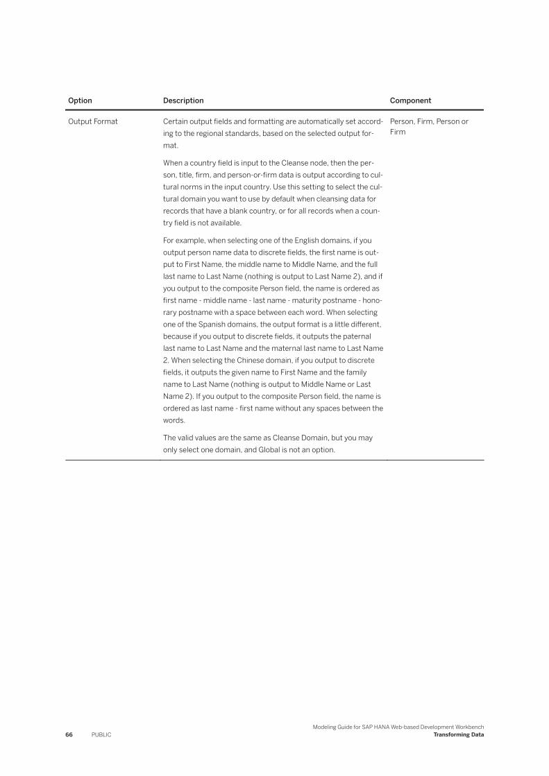
Option Description Component
Output Format Certain output fields and formatting are automatically set according to the regional standards, based on the selected output format.
When a country field is input to the Cleanse node, then the person, title, firm, and person-or-firm data is output according to cultural norms in the input country. Use this setting to select the cultural domain you want to use by default when cleansing data for records that have a blank country, or for all records when a country field is not available.
For example, when selecting one of the English domains, if you output person name data to discrete fields, the first name is output to First Name, the middle name to Middle Name, and the full last name to Last Name (nothing is output to Last Name 2), and if you output to the composite Person field, the name is ordered as first name - middle name - last name - maturity postname - honorary postname with a space between each word. When selecting one of the Spanish domains, the output format is a little different, because if you output to discrete fields, it outputs the paternal last name to Last Name and the maternal last name to Last Name 2. When selecting the Chinese domain, if you output to discrete fields, it outputs the given name to First Name and the family name to Last Name (nothing is output to Middle Name or Last Name 2). If you output to the composite Person field, the name is ordered as last name - first name without any spaces between the words.
The valid values are the same as Cleanse Domain, but you may only select one domain, and Global is not an option.
Person, Firm, Person or Firm
66 PUBLICModeling Guide for SAP HANA Web-based Development Workbench
Transforming Data

Option Description Component
Postal Format Specifies how to format postal box addresses.
NoteIn some countries it is not acceptable to fully spell out the form of the postal address. In other countries, it is not acceptable to include periods in the abbreviated form. In these cases, the cleansed addresses meet the country-specific requirements, even when you select a different option.
Abbreviate No Punctuation: Uses a shortened form of the postal address without punctuation. For example, PO Box 101.
Abbreviate With Punctuation: Uses a shortened form of the postal address with punctuation. For example, P.O. Box 101.
Expand: Uses the full form of the postal address. For example, Post Office Box 101.
Most common for each country: Uses the most common format of the country where the address is located. For example, in the USA, the preferred format is short without punctuation.
Address
Region Format Specifies how to format the region name (for example, state or province).
Abbreviate: Abbreviate the region name. For example, SC.
NoteIn some countries it is not acceptable to abbreviate region names. In those cases, the cleansed region is fully spelled out, even when you set the option to abbreviate.
Expand: Fully spell out the region name. For example, South Carolina.
Most common for each country: Uses the most common format of the country where the address is located. For example, in the UK, the preferred format is to fully spell out the name of the town in capital letters.
Address
Script Conversion Specifies the script to output addresses in China, Taiwan, Republic of Korea, and Russian Federation.
Convert to Latin: Converts non-Latin scripts so that all of the output data is in Latin script.
Preserve Input: Retains all scripts as they were input. If you have input data in a variety of scripts, then the original script for those records are output in the same script.
Address
Modeling Guide for SAP HANA Web-based Development WorkbenchTransforming Data PUBLIC 67
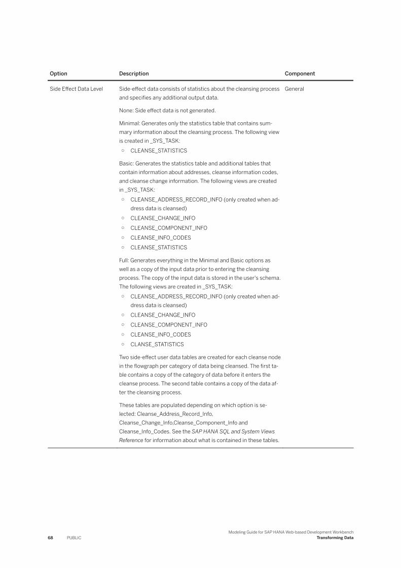
Option Description Component
Side Effect Data Level Side-effect data consists of statistics about the cleansing process and specifies any additional output data.
None: Side effect data is not generated.
Minimal: Generates only the statistics table that contains summary information about the cleansing process. The following view is created in _SYS_TASK:○ CLEANSE_STATISTICS
Basic: Generates the statistics table and additional tables that contain information about addresses, cleanse information codes, and cleanse change information. The following views are created in _SYS_TASK:○ CLEANSE_ADDRESS_RECORD_INFO (only created when ad
dress data is cleansed)○ CLEANSE_CHANGE_INFO○ CLEANSE_COMPONENT_INFO○ CLEANSE_INFO_CODES○ CLEANSE_STATISTICS
Full: Generates everything in the Minimal and Basic options as well as a copy of the input data prior to entering the cleansing process. The copy of the input data is stored in the user's schema. The following views are created in _SYS_TASK:○ CLEANSE_ADDRESS_RECORD_INFO (only created when ad
dress data is cleansed)○ CLEANSE_CHANGE_INFO○ CLEANSE_COMPONENT_INFO○ CLEANSE_INFO_CODES○ CLANSE_STATISTICS
Two side-effect user data tables are created for each cleanse node in the flowgraph per category of data being cleansed. The first table contains a copy of the category of data before it enters the cleanse process. The second table contains a copy of the data after the cleansing process.
These tables are populated depending on which option is selected: Cleanse_Address_Record_Info, Cleanse_Change_Info,Cleanse_Component_Info and Cleanse_Info_Codes. See the SAP HANA SQL and System Views Reference for information about what is contained in these tables.
General
68 PUBLICModeling Guide for SAP HANA Web-based Development Workbench
Transforming Data
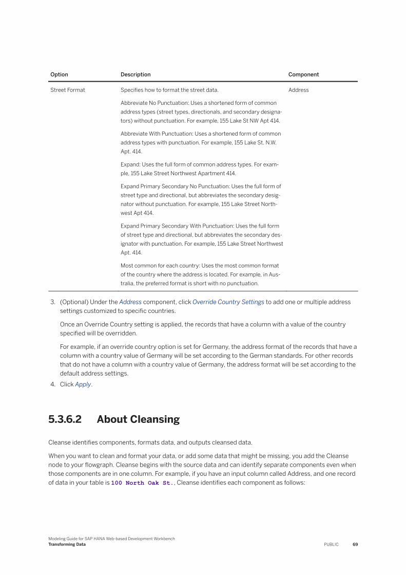
Option Description Component
Street Format Specifies how to format the street data.
Abbreviate No Punctuation: Uses a shortened form of common address types (street types, directionals, and secondary designators) without punctuation. For example, 155 Lake St NW Apt 414.
Abbreviate With Punctuation: Uses a shortened form of common address types with punctuation. For example, 155 Lake St. N.W. Apt. 414.
Expand: Uses the full form of common address types. For example, 155 Lake Street Northwest Apartment 414.
Expand Primary Secondary No Punctuation: Uses the full form of street type and directional, but abbreviates the secondary designator without punctuation. For example, 155 Lake Street Northwest Apt 414.
Expand Primary Secondary With Punctuation: Uses the full form of street type and directional, but abbreviates the secondary designator with punctuation. For example, 155 Lake Street Northwest Apt. 414.
Most common for each country: Uses the most common format of the country where the address is located. For example, in Australia, the preferred format is short with no punctuation.
Address
3. (Optional) Under the Address component, click Override Country Settings to add one or multiple address settings customized to specific countries.
Once an Override Country setting is applied, the records that have a column with a value of the country specified will be overridden.
For example, if an override country option is set for Germany, the address format of the records that have a column with a country value of Germany will be set according to the German standards. For other records that do not have a column with a country value of Germany, the address format will be set according to the default address settings.
4. Click Apply.
5.3.6.2 About Cleansing
Cleanse identifies components, formats data, and outputs cleansed data.
When you want to clean and format your data, or add some data that might be missing, you add the Cleanse node to your flowgraph. Cleanse begins with the source data and can identify separate components even when those components are in one column. For example, if you have an input column called Address, and one record of data in your table is 100 North Oak St., Cleanse identifies each component as follows:
Modeling Guide for SAP HANA Web-based Development WorkbenchTransforming Data PUBLIC 69
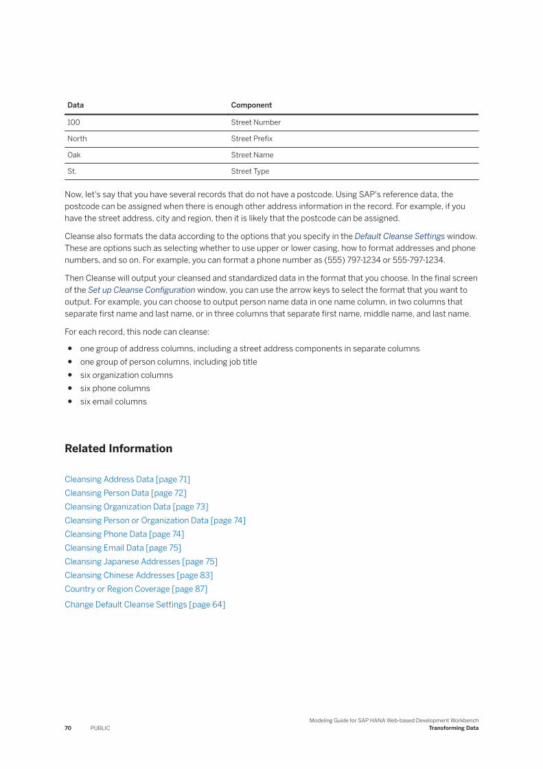
Data Component
100 Street Number
North Street Prefix
Oak Street Name
St. Street Type
Now, let's say that you have several records that do not have a postcode. Using SAP's reference data, the postcode can be assigned when there is enough other address information in the record. For example, if you have the street address, city and region, then it is likely that the postcode can be assigned.
Cleanse also formats the data according to the options that you specify in the Default Cleanse Settings window. These are options such as selecting whether to use upper or lower casing, how to format addresses and phone numbers, and so on. For example, you can format a phone number as (555) 797-1234 or 555-797-1234.
Then Cleanse will output your cleansed and standardized data in the format that you choose. In the final screen of the Set up Cleanse Configuration window, you can use the arrow keys to select the format that you want to output. For example, you can choose to output person name data in one name column, in two columns that separate first name and last name, or in three columns that separate first name, middle name, and last name.
For each record, this node can cleanse:
● one group of address columns, including a street address components in separate columns● one group of person columns, including job title● six organization columns● six phone columns● six email columns
Related Information
Cleansing Address Data [page 71]Cleansing Person Data [page 72]Cleansing Organization Data [page 73]Cleansing Person or Organization Data [page 74]Cleansing Phone Data [page 74]Cleansing Email Data [page 75]Cleansing Japanese Addresses [page 75]Cleansing Chinese Addresses [page 83]Country or Region Coverage [page 87]
Change Default Cleanse Settings [page 64]
70 PUBLICModeling Guide for SAP HANA Web-based Development Workbench
Transforming Data
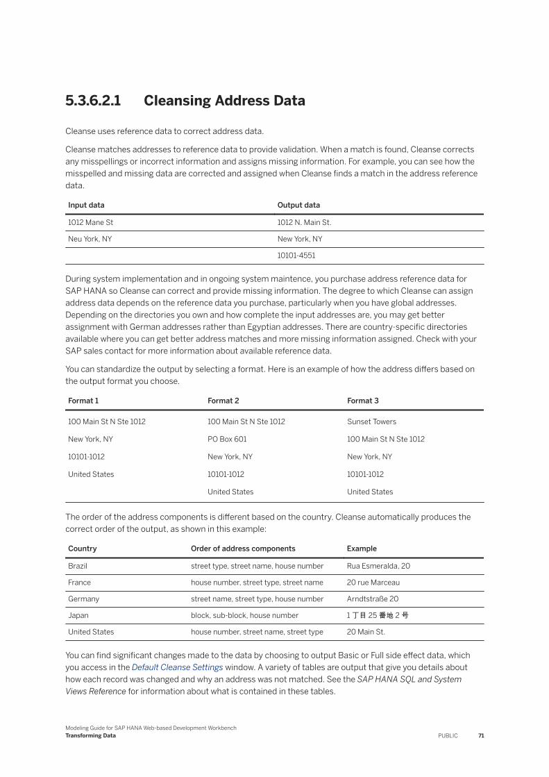
5.3.6.2.1 Cleansing Address Data
Cleanse uses reference data to correct address data.
Cleanse matches addresses to reference data to provide validation. When a match is found, Cleanse corrects any misspellings or incorrect information and assigns missing information. For example, you can see how the misspelled and missing data are corrected and assigned when Cleanse finds a match in the address reference data.
Input data Output data
1012 Mane St 1012 N. Main St.
Neu York, NY New York, NY
10101-4551
During system implementation and in ongoing system maintence, you purchase address reference data for SAP HANA so Cleanse can correct and provide missing information. The degree to which Cleanse can assign address data depends on the reference data you purchase, particularly when you have global addresses. Depending on the directories you own and how complete the input addresses are, you may get better assignment with German addresses rather than Egyptian addresses. There are country-specific directories available where you can get better address matches and more missing information assigned. Check with your SAP sales contact for more information about available reference data.
You can standardize the output by selecting a format. Here is an example of how the address differs based on the output format you choose.
Format 1 Format 2 Format 3
100 Main St N Ste 1012
New York, NY
10101-1012
United States
100 Main St N Ste 1012
PO Box 601
New York, NY
10101-1012
United States
Sunset Towers
100 Main St N Ste 1012
New York, NY
10101-1012
United States
The order of the address components is different based on the country. Cleanse automatically produces the correct order of the output, as shown in this example:
Country Order of address components Example
Brazil street type, street name, house number Rua Esmeralda, 20
France house number, street type, street name 20 rue Marceau
Germany street name, street type, house number Arndtstraße 20
Japan block, sub-block, house number 1 丁目 25 番地 2 号
United States house number, street name, street type 20 Main St.
You can find significant changes made to the data by choosing to output Basic or Full side effect data, which you access in the Default Cleanse Settings window. A variety of tables are output that give you details about how each record was changed and why an address was not matched. See the SAP HANA SQL and System Views Reference for information about what is contained in these tables.
Modeling Guide for SAP HANA Web-based Development WorkbenchTransforming Data PUBLIC 71
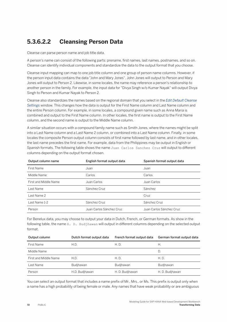
5.3.6.2.2 Cleansing Person DataCleanse can parse person name and job title data.
A person's name can consist of the following parts: prename, first names, last names, postnames, and so on. Cleanse can identify individual components and standardize the data to the output format that you choose.
Cleanse input mapping can map to one job title column and one group of person name columns. However, if the person input data contains the data "John and Mary Jones", John Jones will output to Person and Mary Jones will output to Person 2. Likewise, in some locales, the name may reference a person's relationship to another person in the family. For example, the input data for "Divya Singh w/o Kumar Nayak" will output Divya Singh to Person and Kumar Nayak to Person 2.
Cleanse also standardizes the names based on the regional domain that you select in the Edit Default Cleanse Settings window. This changes how the data is output for the First Name column and Last Name column and the entire Person column. For example, in some locales, a compound given name such as Anna Maria is combined and output to the First Name column. In other locales, the first name is output to the First Name column, and the second name is output to the Middle Name column.
A similar situation occurs with a compound family name such as Smith Jones, where the names might be split into a Last Name column and a Last Name 2 column, or combined into a Last Name column. Finally, in some locales the composite Person output column consists of first name followed by last name, and in other locales, the last name precedes the first name. For example, data from the Philippines may be output in English or Spanish formats. The following table shows the name Juan Carlos Sanchez Cruz will output to different columns depending on the output format chosen.
Output column name English format output data Spanish format output data
First Name Juan Juan
Middle Name Carlos Carlos
First and Middle Name Juan Carlos Juan Carlos
Last Name Sánchez Cruz Sánchez
Last Name 2 Cruz
Last Name 1-2 Sánchez Cruz Sánchez Cruz
Person Juan Carlos Sánchez Cruz Juan Carlos Sánchez Cruz
For Benelux data, you may choose to output your data in Dutch, French, or German formats. As show in the following table, the name H. D. Budjhawan will output in different columns depending on the selected output format.
Output column Dutch format output data French format output data German format output data
First Name H.D. H. D. H.
Middle Name D.
First and Middle Name H.D. H. D. H. D.
Last Name Budjhawan Budjhawan Budjhawan
Person H.D. Budjhawan H. D. Budjhawan H. D. Budjhawan
You can select an output format that includes a name prefix of Mr., Mrs., or Ms. This prefix is output only when a name has a high probability of being female or male. Any names that have weak probability or are ambiguous
72 PUBLICModeling Guide for SAP HANA Web-based Development Workbench
Transforming Data
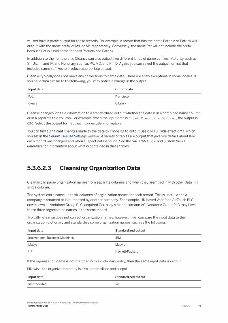
will not have a prefix output for those records. For example, a record that has the name Patricia or Patrick will output with the name prefix of Ms. or Mr. respectively. Conversely, the name Pat will not include the prefix because Pat is a nickname for both Patricia and Patrick.
In addition to the name prefix, Cleanse can also output two different kinds of name suffixes: Maturity such as Sr., Jr., III, and IV, and Honorary such as PA, MD, and Ph. D. Again, you can select the output format that includes name suffixes to produce appropriate output.
Cleanse typically does not make any corrections to name data. There are a few exceptions in some locales. If you have data similar to the following, you may notice a change in the output:
Input data Output data
Fco. Francisco
Oleary O'Leary
Cleanse changes job title information to a standardized output whether the data is in a combined name column or in a separate title column. For example, when the input data is Chief Executive Officer, the output is CEO. Select the output format that includes title information.
You can find significant changes made to the data by choosing to output Basic or Full side effect data, which you set in the Default Cleanse Settings window. A variety of tables are output that give you details about how each record was changed and when suspect data is found. See the SAP HANA SQL and System Views Reference for information about what is contained in these tables.
5.3.6.2.3 Cleansing Organization Data
Cleanse can parse organization names from separate columns and when they aremixed in with other data in a single column.
The system can cleanse up to six columns of organization names for each record. This is useful when a company is renamed or is purchased by another company. For example, UK-based Vodafone AirTouch PLC, now known as Vodafone Group PLC, acquired Germany's Mannesamann AG. Vodafone Group PLC may have those three organization names in the same record.
Typically, Cleanse does not correct organization names, however, it will compare the input data to the organization dictionary and standardize some organization names, such as the following:
Input data Standardized output
International Business Machines IBM
Macys Macy's
HP Hewlett-Packard
If the organization name is not matched with a dictionary entry, then the same input data is output.
Likewise, the organization entity is also standardized and output.
Input data Standardized output
Incorporated Inc.
Modeling Guide for SAP HANA Web-based Development WorkbenchTransforming Data PUBLIC 73
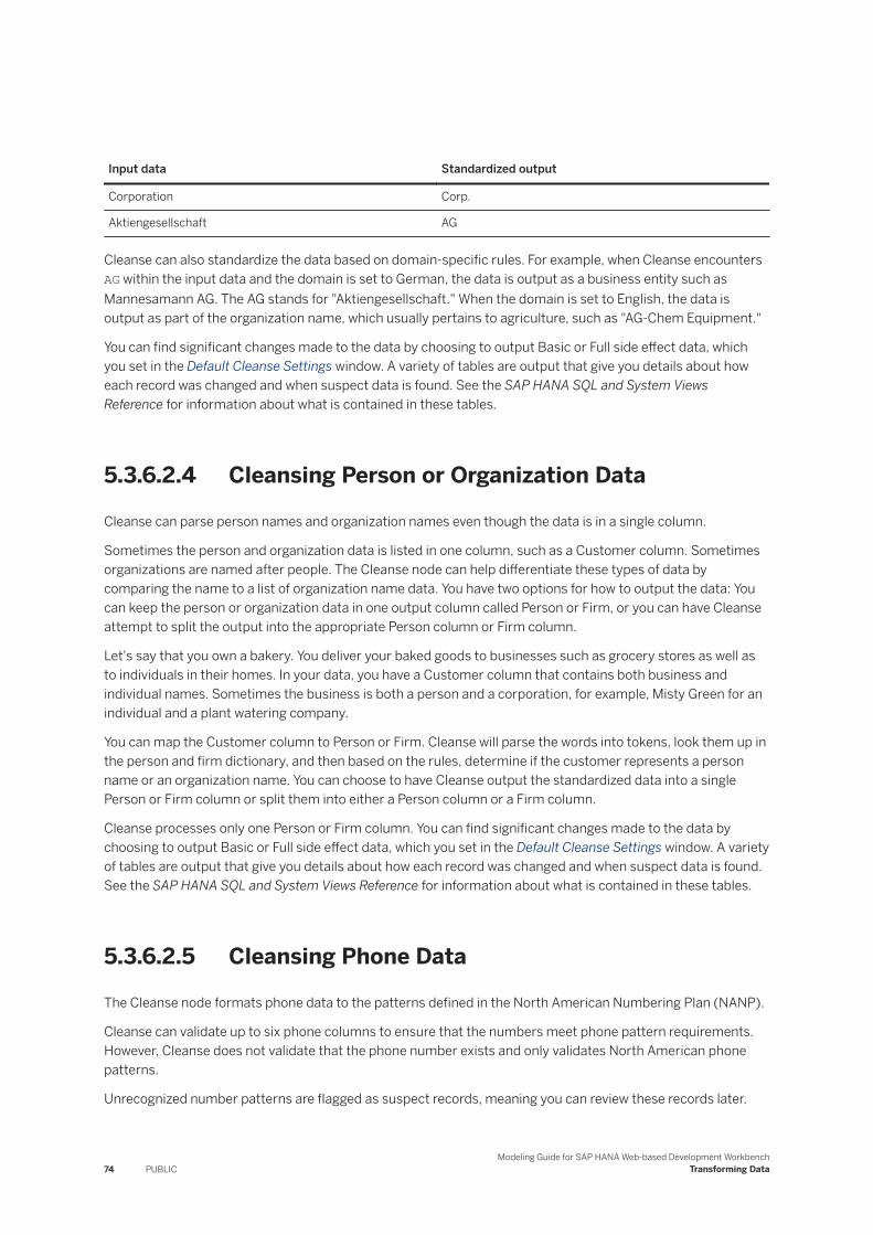
Input data Standardized output
Corporation Corp.
Aktiengesellschaft AG
Cleanse can also standardize the data based on domain-specific rules. For example, when Cleanse encounters AG within the input data and the domain is set to German, the data is output as a business entity such as Mannesamann AG. The AG stands for "Aktiengesellschaft." When the domain is set to English, the data is output as part of the organization name, which usually pertains to agriculture, such as "AG-Chem Equipment."
You can find significant changes made to the data by choosing to output Basic or Full side effect data, which you set in the Default Cleanse Settings window. A variety of tables are output that give you details about how each record was changed and when suspect data is found. See the SAP HANA SQL and System Views Reference for information about what is contained in these tables.
5.3.6.2.4 Cleansing Person or Organization Data
Cleanse can parse person names and organization names even though the data is in a single column.
Sometimes the person and organization data is listed in one column, such as a Customer column. Sometimes organizations are named after people. The Cleanse node can help differentiate these types of data by comparing the name to a list of organization name data. You have two options for how to output the data: You can keep the person or organization data in one output column called Person or Firm, or you can have Cleanse attempt to split the output into the appropriate Person column or Firm column.
Let's say that you own a bakery. You deliver your baked goods to businesses such as grocery stores as well as to individuals in their homes. In your data, you have a Customer column that contains both business and individual names. Sometimes the business is both a person and a corporation, for example, Misty Green for an individual and a plant watering company.
You can map the Customer column to Person or Firm. Cleanse will parse the words into tokens, look them up in the person and firm dictionary, and then based on the rules, determine if the customer represents a person name or an organization name. You can choose to have Cleanse output the standardized data into a single Person or Firm column or split them into either a Person column or a Firm column.
Cleanse processes only one Person or Firm column. You can find significant changes made to the data by choosing to output Basic or Full side effect data, which you set in the Default Cleanse Settings window. A variety of tables are output that give you details about how each record was changed and when suspect data is found. See the SAP HANA SQL and System Views Reference for information about what is contained in these tables.
5.3.6.2.5 Cleansing Phone Data
The Cleanse node formats phone data to the patterns defined in the North American Numbering Plan (NANP).
Cleanse can validate up to six phone columns to ensure that the numbers meet phone pattern requirements. However, Cleanse does not validate that the phone number exists and only validates North American phone patterns.
Unrecognized number patterns are flagged as suspect records, meaning you can review these records later.
74 PUBLICModeling Guide for SAP HANA Web-based Development Workbench
Transforming Data
You can find significant changes made to the data by choosing to output Basic or Full side effect data, which you set in the Default Cleanse Settings window. A variety of tables are output that give you details about how each record was changed and when suspect data is found. See the SAP HANA SQL and System Views Reference for information about what is contained in these tables.
5.3.6.2.6 Cleansing Email Data
The Cleanse node formats email addresses according to email settings.
Use Cleanse to validate up to six email columns to ensure that they meet email pattern requirements and to verify that the email address is properly formatted.
Cleanse does not verify the following:
● whether the domain name, which isthe portion after the @ sign, is registered● whether an email server is active at that address● whether the user name, which isthe portion before the @ sign, is registered on that email server● whether the person's name in the record can be reached at this email address
You can find significant changes made to the data by choosing to output Basic or Full side effect data, which you set in the Default Cleanse Settings window. A variety of tables are output that give you details about how each record was changed and when suspect data is found. See the SAP HANA SQL and System Views Reference for information about what is contained in these tables.
5.3.6.2.7 Cleansing Japanese Addresses
Using the Japanese directories, you can cleanse and normalize person and address data for matching.
A significant portion of the address parsing capability relies on the Japanese address database. The software has data from the Ministry of Public Management, Home Affairs, Posts and Telecommunications (MPT) and additional data sources. The enhanced address database consists of a regularly updated government database that includes regional postal codes mapped to localities.
NoteThe Japan engine supports only kanji and katakana data. The engine does not support Latin data.
To use the Japan engine and directories:
1. Click Edit Cleanse Settings.
2. Choose Edit Defaults Edit Settings .3. Set the Cleanse Domain and Output Format to JA (Japanese).
Related Information
Standard Japanese Address Format [page 76]
Modeling Guide for SAP HANA Web-based Development WorkbenchTransforming Data PUBLIC 75

Additional Japanese Address Formats [page 80]Special Hokkaido Regional Formats [page 81]Japanese Address Example [page 81]
5.3.6.2.7.1 Standard Japanese Address Format
A typical Japanese address includes these components.
Address component Japanese example English example Output column
Postcode 〒 654-0153 654-0153 Postcode
Prefecture 兵庫県 Hyogo-ken Region (Expanded)
City 神戸市 Kobe-shi City (Expanded)
Ward 須磨区 Suma-ku Subcity (Expanded)
District 南落合 Minami Ochiai Subcity 2-3 (Expanded)
Block number 1 丁目 1 chome Street Name 1-2
Sub-block number 25 番地 25 banchi Street Name 3-4
House number 2 号 2 go Street Number (Expanded)
An address may also include a building name, floor number, or room number.
Related Information
Japanese Address Components [page 76]Common Building Name Suffixes [page 79]Japanese Building Number Examples [page 80]
5.3.6.2.7.1.1 Japanese Address Components
Descriptions of each component in a Japanese address.
Japanese address component Description
Postcode Japanese postal codes are in the nnn-nnnn format. The first three digits represent the area. The last four digits represent a location in the area. The possible locations are district, sub-district, block, sub-block, building, floor, and company. Postal codes must be written with Arabic numbers. The post office symbol 〒 is optional.
Before 1998, the postal code consisted of 3 or 5 digits. Some older databases may still reflect the old format.
76 PUBLICModeling Guide for SAP HANA Web-based Development Workbench
Transforming Data
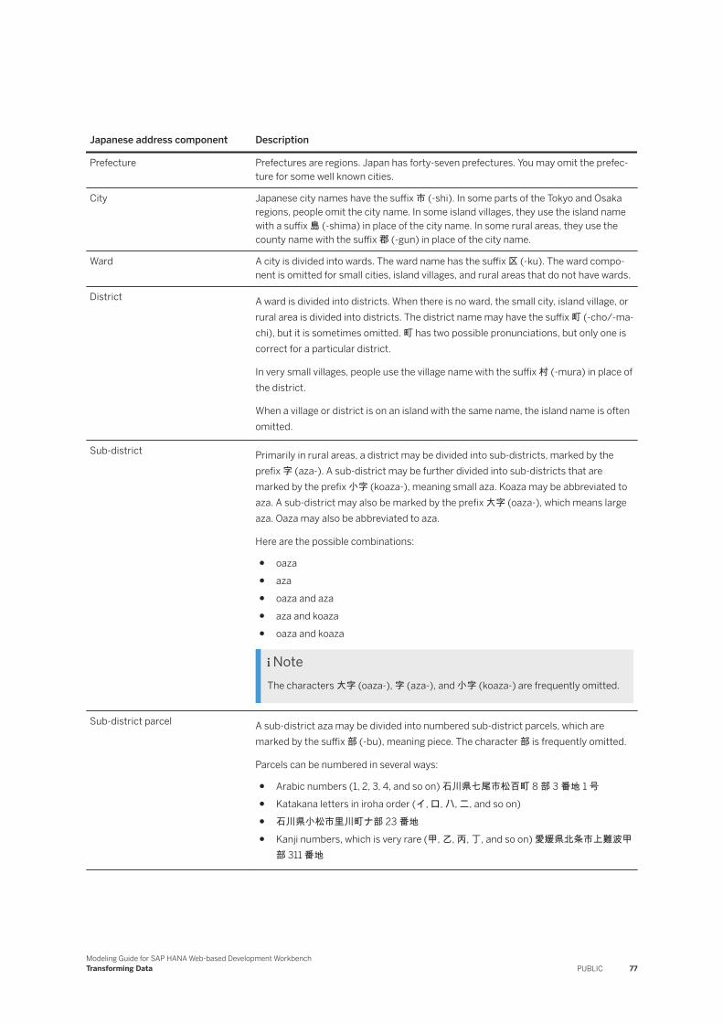
Japanese address component Description
Prefecture Prefectures are regions. Japan has forty-seven prefectures. You may omit the prefecture for some well known cities.
City Japanese city names have the suffix 市 (-shi). In some parts of the Tokyo and Osaka regions, people omit the city name. In some island villages, they use the island name with a suffix 島 (-shima) in place of the city name. In some rural areas, they use the county name with the suffix 郡 (-gun) in place of the city name.
Ward A city is divided into wards. The ward name has the suffix 区 (-ku). The ward component is omitted for small cities, island villages, and rural areas that do not have wards.
District A ward is divided into districts. When there is no ward, the small city, island village, or rural area is divided into districts. The district name may have the suffix 町 (-cho/-machi), but it is sometimes omitted. 町 has two possible pronunciations, but only one is correct for a particular district.
In very small villages, people use the village name with the suffix 村 (-mura) in place of the district.
When a village or district is on an island with the same name, the island name is often omitted.
Sub-district Primarily in rural areas, a district may be divided into sub-districts, marked by the prefix 字 (aza-). A sub-district may be further divided into sub-districts that are marked by the prefix 小字 (koaza-), meaning small aza. Koaza may be abbreviated to aza. A sub-district may also be marked by the prefix 大字 (oaza-), which means large aza. Oaza may also be abbreviated to aza.
Here are the possible combinations:
● oaza● aza● oaza and aza● aza and koaza● oaza and koaza
NoteThe characters 大字 (oaza-), 字 (aza-), and 小字 (koaza-) are frequently omitted.
Sub-district parcel A sub-district aza may be divided into numbered sub-district parcels, which are marked by the suffix 部 (-bu), meaning piece. The character 部 is frequently omitted.
Parcels can be numbered in several ways:
● Arabic numbers (1, 2, 3, 4, and so on) 石川県七尾市松百町 8 部 3 番地 1 号
● Katakana letters in iroha order (イ, ロ, ハ, ニ, and so on)● 石川県小松市里川町ナ部 23 番地
● Kanji numbers, which is very rare (甲, 乙, 丙, 丁, and so on) 愛媛県北条市上難波甲部 311 番地
Modeling Guide for SAP HANA Web-based Development WorkbenchTransforming Data PUBLIC 77
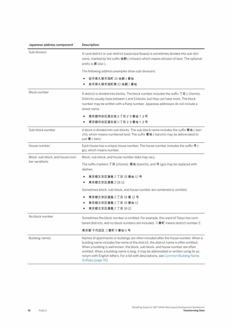
Japanese address component Description
Sub-division A rural district or sub-district (oaza/aza/koaza) is sometimes divided into sub-divisions, marked by the suffix 地割 (-chiwari) which means division of land. The optional prefix is 第 (dai-).
The following address examples show sub-divisions:
● 岩手県久慈市旭町 10 地割 1 番地
● 岩手県久慈市旭町第 10 地割 1 番地
Block number A district is divided into blocks. The block number includes the suffix 丁目 (-chome). Districts usually have between 1 and 5 blocks, but they can have more. The block number may be written with a Kanji number. Japanese addresses do not include a street name.
● 東京都渋谷区道玄坂2丁目25番地12号
● 東京都渋谷区道玄坂二丁目25番地12号
Sub-block number A block is divided into sub-blocks. The sub-block name includes the suffix 番地 (-banchi), which means numbered land. The suffix 番地 (-banchi) may be abbreviated to just 番 (-ban).
House number Each house has a unique house number. The house number includes the suffix 号 (-go), which means number.
Block, sub-block, and house number variations
Block, sub-block, and house number data may vary.
The suffix markers 丁目 (chome), 番地 (banchi), and 号 (go) may be replaced with dashes.
● 東京都文京区湯島 2 丁目 18 番地 12 号
● 東京都文京区湯島 2-18-12
Sometimes block, sub-block, and house number are combined or omitted.
● 東京都文京区湯島 2 丁目 18 番 12 号
● 東京都文京区湯島 2 丁目 18 番地 12● 東京都文京区湯島 2 丁目 18-12
No block number Sometimes the block number is omitted. For example, this ward of Tokyo has numbered districts, and no block numbers are included. 二番町 means district number 2.
東京都 千代田区 二番町 9 番地 6 号
Building names Names of apartments or buildings are often included after the house number. When a building name includes the name of the district, the district name is often omitted. When a building is well known, the block, sub-block, and house number are often omitted. When a building name is long, it may be abbreviated or written using its acronym with English letters. For a list with descriptions, see Common Building Name Suffixes [page 79].
78 PUBLICModeling Guide for SAP HANA Web-based Development Workbench
Transforming Data
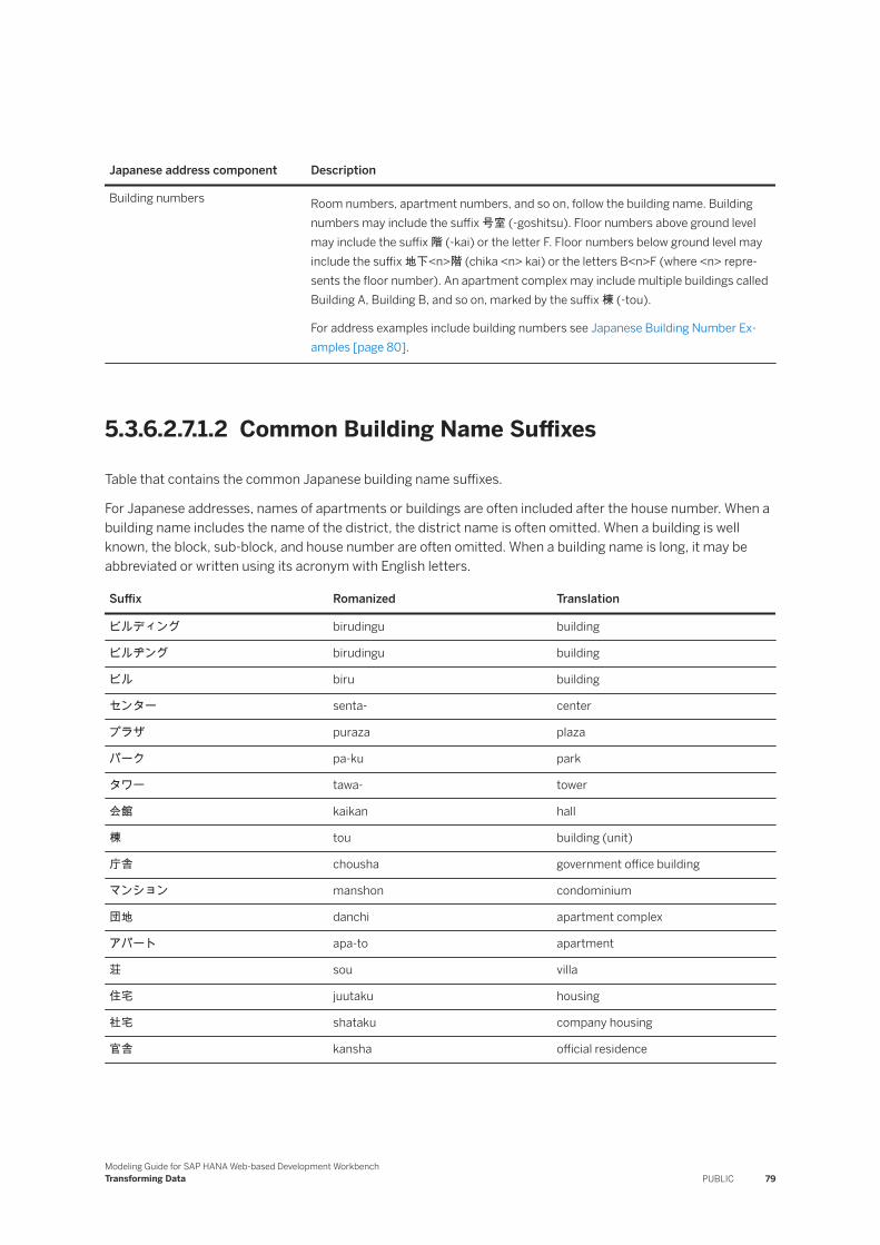
Japanese address component Description
Building numbers Room numbers, apartment numbers, and so on, follow the building name. Building numbers may include the suffix 号室 (-goshitsu). Floor numbers above ground level may include the suffix 階 (-kai) or the letter F. Floor numbers below ground level may include the suffix 地下<n>階 (chika <n> kai) or the letters B<n>F (where <n> represents the floor number). An apartment complex may include multiple buildings called Building A, Building B, and so on, marked by the suffix 棟 (-tou).
For address examples include building numbers see Japanese Building Number Examples [page 80].
5.3.6.2.7.1.2 Common Building Name Suffixes
Table that contains the common Japanese building name suffixes.
For Japanese addresses, names of apartments or buildings are often included after the house number. When a building name includes the name of the district, the district name is often omitted. When a building is well known, the block, sub-block, and house number are often omitted. When a building name is long, it may be abbreviated or written using its acronym with English letters.
Suffix Romanized Translation
ビルディング birudingu building
ビルヂング birudingu building
ビル biru building
センター senta- center
プラザ puraza plaza
パーク pa-ku park
タワー tawa- tower
会館 kaikan hall
棟 tou building (unit)
庁舎 chousha government office building
マンション manshon condominium
団地 danchi apartment complex
アパート apa-to apartment
荘 sou villa
住宅 juutaku housing
社宅 shataku company housing
官舎 kansha official residence
Modeling Guide for SAP HANA Web-based Development WorkbenchTransforming Data PUBLIC 79
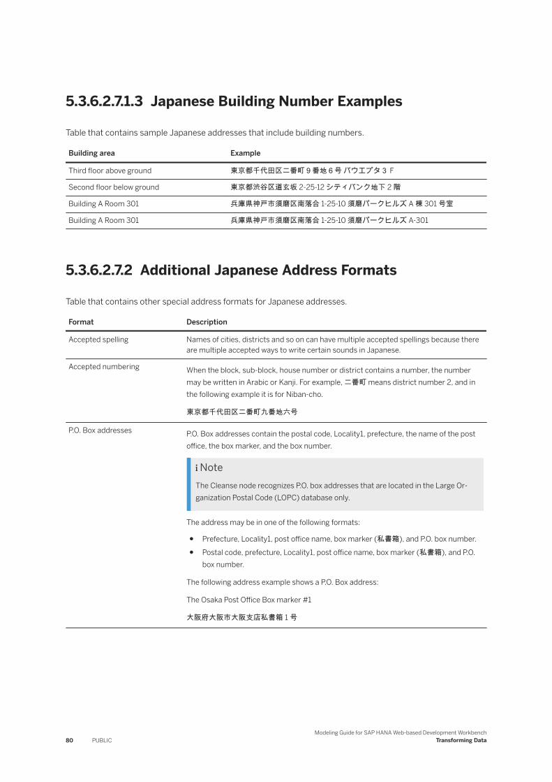
5.3.6.2.7.1.3 Japanese Building Number Examples
Table that contains sample Japanese addresses that include building numbers.
Building area Example
Third floor above ground 東京都千代田区二番町9番地6号 バウエプタ3 F
Second floor below ground 東京都渋谷区道玄坂 2-25-12 シティバンク地下 2 階
Building A Room 301 兵庫県神戸市須磨区南落合 1-25-10 須磨パークヒルズ A 棟 301 号室
Building A Room 301 兵庫県神戸市須磨区南落合 1-25-10 須磨パークヒルズ A-301
5.3.6.2.7.2 Additional Japanese Address Formats
Table that contains other special address formats for Japanese addresses.
Format Description
Accepted spelling Names of cities, districts and so on can have multiple accepted spellings because there are multiple accepted ways to write certain sounds in Japanese.
Accepted numbering When the block, sub-block, house number or district contains a number, the number may be written in Arabic or Kanji. For example, 二番町 means district number 2, and in the following example it is for Niban-cho.
東京都千代田区二番町九番地六号
P.O. Box addresses P.O. Box addresses contain the postal code, Locality1, prefecture, the name of the post office, the box marker, and the box number.
NoteThe Cleanse node recognizes P.O. box addresses that are located in the Large Organization Postal Code (LOPC) database only.
The address may be in one of the following formats:
● Prefecture, Locality1, post office name, box marker (私書箱), and P.O. box number.● Postal code, prefecture, Locality1, post office name, box marker (私書箱), and P.O.
box number.
The following address example shows a P.O. Box address:
The Osaka Post Office Box marker #1
大阪府大阪市大阪支店私書箱 1 号
80 PUBLICModeling Guide for SAP HANA Web-based Development Workbench
Transforming Data
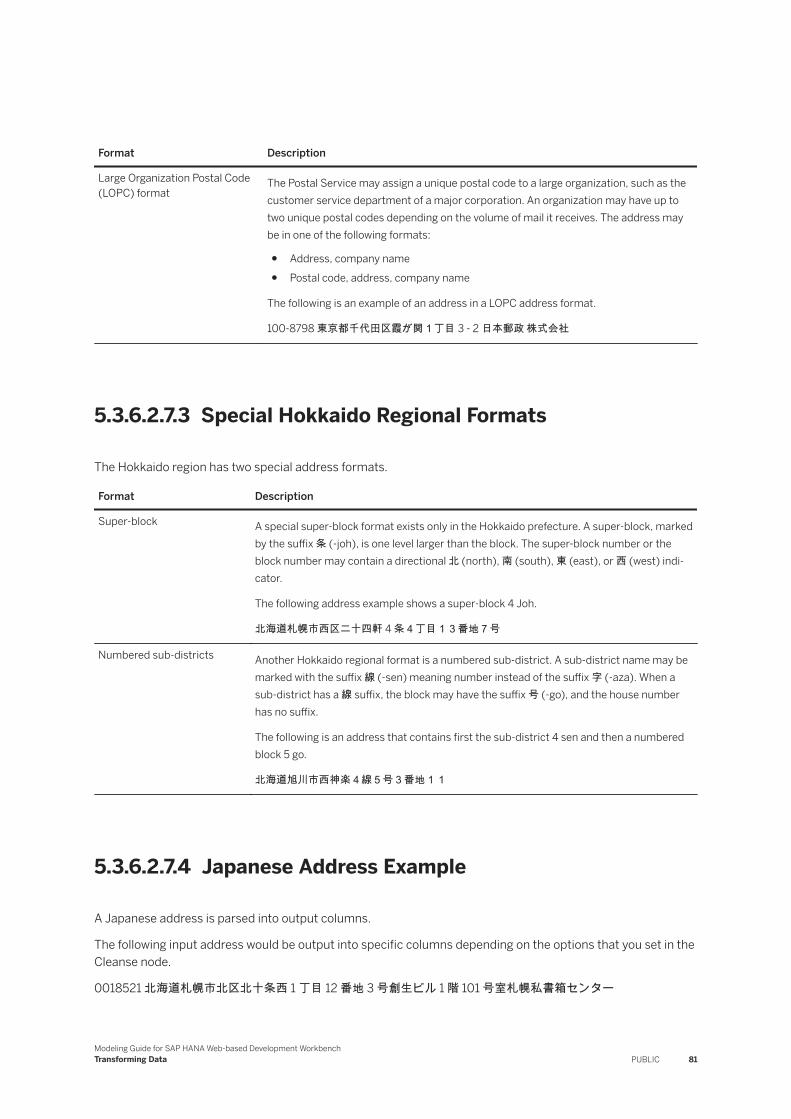
Format Description
Large Organization Postal Code (LOPC) format
The Postal Service may assign a unique postal code to a large organization, such as the customer service department of a major corporation. An organization may have up to two unique postal codes depending on the volume of mail it receives. The address may be in one of the following formats:
● Address, company name● Postal code, address, company name
The following is an example of an address in a LOPC address format.
100-8798 東京都千代田区霞が関1丁目 3 - 2 日本郵政 株式会社
5.3.6.2.7.3 Special Hokkaido Regional Formats
The Hokkaido region has two special address formats.
Format Description
Super-block A special super-block format exists only in the Hokkaido prefecture. A super-block, marked by the suffix 条 (-joh), is one level larger than the block. The super-block number or the block number may contain a directional 北 (north), 南 (south), 東 (east), or 西 (west) indicator.
The following address example shows a super-block 4 Joh.
北海道札幌市西区二十四軒 4 条4丁目13番地7号
Numbered sub-districts Another Hokkaido regional format is a numbered sub-district. A sub-district name may be marked with the suffix 線 (-sen) meaning number instead of the suffix 字 (-aza). When a sub-district has a 線 suffix, the block may have the suffix 号 (-go), and the house number has no suffix.
The following is an address that contains first the sub-district 4 sen and then a numbered block 5 go.
北海道旭川市西神楽4線5号3番地11
5.3.6.2.7.4 Japanese Address Example
A Japanese address is parsed into output columns.
The following input address would be output into specific columns depending on the options that you set in the Cleanse node.
0018521 北海道札幌市北区北十条西 1 丁目 12 番地 3 号創生ビル 1 階 101 号室札幌私書箱センター
Modeling Guide for SAP HANA Web-based Development WorkbenchTransforming Data PUBLIC 81
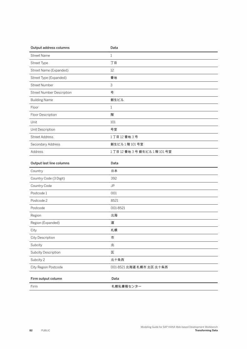
Output address columns Data
Street Name 1
Street Type 丁目
Street Name (Expanded) 12
Street Type (Expanded) 番地
Street Number 3
Street Number Description 号
Building Name 創生ビル
Floor 1
Floor Description 階
Unit 101
Unit Description 号室
Street Address 1 丁目 12 番地 3 号
Secondary Address 創生ビル 1 階 101 号室
Address 1 丁目 12 番地 3 号 創生ビル 1 階 101 号室
Output last line columns Data
Country 日本
Country Code (3 Digit) 392
Country Code JP
Postcode 1 001
Postcode 2 8521
Postcode 001-8521
Region 北海
Region (Expanded) 道
City 札幌
City Description 市
Subcity 北
Subcity Description 区
Subcity 2 北十条西
City Region Postcode 001-8521 北海道 札幌市 北区 北十条西
Firm output column Data
Firm 札幌私書箱センター
82 PUBLICModeling Guide for SAP HANA Web-based Development Workbench
Transforming Data
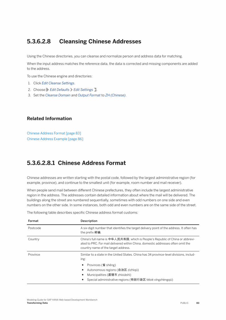
5.3.6.2.8 Cleansing Chinese Addresses
Using the Chinese directories, you can cleanse and normalize person and address data for matching.
When the input address matches the reference data, the data is corrected and missing components are added to the address.
To use the Chinese engine and directories:
1. Click Edit Cleanse Settings.
2. Choose Edit Defaults Edit Settings .3. Set the Cleanse Domain and Output Format to ZH (Chinese).
Related Information
Chinese Address Format [page 83]Chinese Address Example [page 86]
5.3.6.2.8.1 Chinese Address Format
Chinese addresses are written starting with the postal code, followed by the largest administrative region (for example, province), and continue to the smallest unit (for example, room number and mail receiver).
When people send mail between different Chinese prefectures, they often include the largest administrative region in the address. The addresses contain detailed information about where the mail will be delivered. The buildings along the street are numbered sequentially, sometimes with odd numbers on one side and even numbers on the other side. In some instances, both odd and even numbers are on the same side of the street.
The following table describes specific Chinese address format customs:
Format Description
Postcode A six-digit number that identifies the target delivery point of the address. It often has the prefix 邮编.
Country China's full name is 中华人民共和国, which is People's Republic of China or abbreviated to PRC. For mail delivered within China, domestic addresses often omit the country name of the target address.
Province Similar to a state in the United States. China has 34 province-level divisions, including:
● Provinces (省 shěng)● Autonomous regions (自治区 zìzhìqū)● Municipalities (直辖市 zhíxiáshì)● Special administrative regions (特别行政区 tèbié xíngzhèngqū)
Modeling Guide for SAP HANA Web-based Development WorkbenchTransforming Data PUBLIC 83

Format Description
Prefecture Prefecture-level divisions are the second level of the administrative structure, including:
● Prefectures (地区 dìqū)● Autonomous prefectures (自治州 zìzhìzhōu)● Prefecture-level cities (地级市 dìjíshì)● Leagues (盟 méng)
County A sub-division of Prefecture that includes:
● Counties (县 xiàn)● Autonomous counties (自治县 zìzhìxiàn)● County-level cities (县级市 xiànjíshì)● Districts (市辖区 shìxiáqū)● Banners (旗 qí)● Autonomous banners (自治旗 zìzhìqí)● Forestry areas (林区 línqū)● Special districts (特区 tèqū)
Township A Township level division that includes:
● Townships (乡 xiāng)● Ethnic townships (民族乡 mínzúxiāng)● Towns (镇 zhèn)● Subdistricts (街道办事处 jiēdàobànshìchù)● District public offices (区公所 qūgōngsuǒ)● Sumu (苏木 sūmù)● Ethnic sumu (民族苏木 mínzúsūmù)
Village Villages include:
● Neighborhood committees (社区居民委员会 jūmínwěiyuánhùi)● Neighborhoods or communities (社区)● Village committees (村民委员会 cūnmínwěiyuánhùi) or Village groups (村民小组
cūnmínxiǎozǔ)● Administrative villages (行政村 xíngzhèngcūn)
Street information Specifies the delivery point within which the mail receiver can be found. In China, the street information often has the form of street (road) name -> House number. For example, 上海市浦东新区晨晖路 1001 号
● Street name: The street name is usually followed by one of these suffixes 路, 大道, 街, 大街, and so on.
● House number: The house number is followed by the suffix 号; the house number is a unique number on the street/road.
Residential community May be used for mail delivery, especially for some famous residential communities in major cities. The street name and house number might be omitted. The residential community does not have a naming standard and it is not strictly required to be followed by a typical marker. However, it is often followed by typical suffixes such as 新村, 小区, and so on.
Building name Building name is often followed by a building marker such as 大厦, 大楼, though it is not strictly required (for example, 中华大厦). Building name in the residential communities is often represented by a number with a suffix of 号,幢. For example: 上海市浦东新区晨晖路 100 弄 10 号 101 室.
84 PUBLICModeling Guide for SAP HANA Web-based Development Workbench
Transforming Data

Format Description
Common metro address Includes the district name, which is common for metropolitan areas in major cities.
Rural address Includes the village name, which is common for rural addresses.
Related Information
Chinese Metro and Rural Address Components [page 85]
5.3.6.2.8.1.1 Chinese Metro and Rural Address Components
Shows common metro and rural address components.
Common Chinese metro address components
Address component Chinese example English example
Postcode 510030 510030
Country 中国 China
Province 广东省 Guangdong Province
City name 广州市 Guangzhou City
District name 越秀区 Yuexiu District
Street name 西湖路 Xihu Road
House number 99 号 No. 99
Common Chinese rural address components
Address component Chinese example English example
Postcode 5111316 5111316
Country 中国 China
Province 广东省 Guangdong Province
City name 广州市 Guangzhou City
County-level City name 增城市 Zengcheng City
Town name 荔城镇 Licheng Town
Village name 联益村 Lianyi Village
Street name 光大路 Guangda Road
House number 99 号 No. 99
Modeling Guide for SAP HANA Web-based Development WorkbenchTransforming Data PUBLIC 85
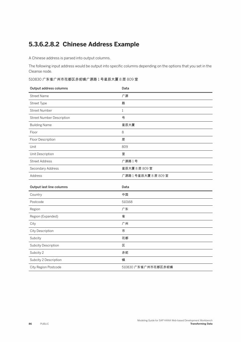
5.3.6.2.8.2 Chinese Address Example
A Chinese address is parsed into output columns.
The following input address would be output into specific columns depending on the options that you set in the Cleanse node.
510830 广东省广州市花都区赤坭镇广源路 1 号星辰大厦 8 层 809 室
Output address columns Data
Street Name 广源
Street Type 路
Street Number 1
Street Number Description 号
Building Name 星辰大厦
Floor 8
Floor Description 层
Unit 809
Unit Description 室
Street Address 广源路 1 号
Secondary Address 星辰大厦 8 层 809 室
Address 广源路 1 号星辰大厦 8 层 809 室
Output last line columns Data
Country 中国
Postcode 510168
Region 广东
Region (Expanded) 省
City 广州
City Description 市
Subcity 花都
Subcity Description 区
Subcity 2 赤坭
Subcity 2 Description 镇
City Region Postcode 510830 广东省广州市花都区赤坭镇
86 PUBLICModeling Guide for SAP HANA Web-based Development Workbench
Transforming Data
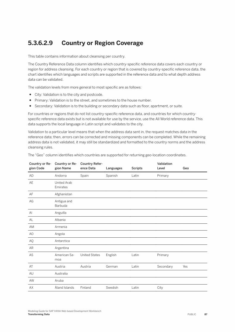
5.3.6.2.9 Country or Region Coverage
This table contains information about cleansing per country.
The Country Reference Data column identifies which country-specific reference data covers each country or region for address cleansing. For each country or region that is covered by country-specific reference data, the chart identifies which languages and scripts are supported in the reference data and to what depth address data can be validated.
The validation levels from more general to most specific are as follows:
● City: Validation is to the city and postcode.● Primary: Validation is to the street, and sometimes to the house number.● Secondary: Validation is to the building or secondary data such as floor, apartment, or suite.
For countries or regions that do not list country-specific reference data, and countries for which country-specific reference data exists but is not available for use by the service, use the All World reference data. This data supports the local language in Latin script and validates to the city.
Validation to a particular level means that when the address data sent in, the request matches data in the reference data; then, errors can be corrected and missing components can be completed. While the remaining address data is not validated, it may still be standardized and formatted to the country norms and the address cleansing rules.
The “Geo” column identifies which countries are supported for returning geo-location coordinates.
Country or Region Code
Country or Region Name
Country Reference Data Languages Scripts
Validation Level Geo
AD Andorra Spain Spanish Latin Primary
AE United Arab Emirates
AF Afghanistan
AG Antigua and Barbuda
AI Anguilla
AL Albania
AM Armenia
AO Angola
AQ Antarctica
AR Argentina
AS American Samoa
United States English Latin Primary
AT Austria Austria German Latin Secondary Yes
AU Australia
AW Aruba
AX Åland Islands Finland Swedish Latin City
Modeling Guide for SAP HANA Web-based Development WorkbenchTransforming Data PUBLIC 87

Country or Region Code
Country or Region Name
Country Reference Data Languages Scripts
Validation Level Geo
AZ Azerbaijan
BA Bosnia and Herzegovina
BB Barbados
BD Bangladesh
BE Belgium Belgium Dutch, French, German
Latin Primary Yes
BF Burkina Faso
BG Bulgaria
BH Bahrain
BI Burundi
BJ Benin
BM Bermuda
BL Saint Barthélemy
France French Latin Primary
BN Brunei Darussalam
BO Plurinational State of Bolivia
BQ Bonaire, Sint Eustatius, and Saba
BR Brazil Brazil Portuguese Latin Primary Yes
BS Bahamas (the)
BT Bhutan
BV Bouvet Island
BW Botswana
BY Belarus
BZ Belize
CA Canada Canada English, French Latin Secondary Yes
CC Cocos (Keeling) Islands
CD Congo (Democratic Republic of the)
CF Central African Republic (the)
88 PUBLICModeling Guide for SAP HANA Web-based Development Workbench
Transforming Data
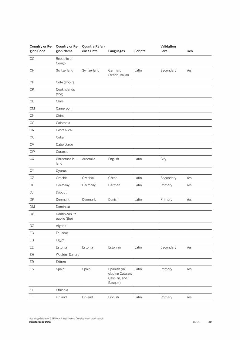
Country or Region Code
Country or Region Name
Country Reference Data Languages Scripts
Validation Level Geo
CG Republic of Congo
CH Switzerland Switzerland German, French, Italian
Latin Secondary Yes
CI Côte d'Ivoire
CK Cook Islands (the)
CL Chile
CM Cameroon
CN China
CO Colombia
CR Costa Rica
CU Cuba
CV Cabo Verde
CW Curaçao
CX Christmas Island
Australia English Latin City
CY Cyprus
CZ Czechia Czechia Czech Latin Secondary Yes
DE Germany Germany German Latin Primary Yes
DJ Djibouti
DK Denmark Denmark Danish Latin Primary Yes
DM Dominica
DO Dominican Republic (the)
DZ Algeria
EC Ecuador
EG Egypt
EE Estonia Estonia Estonian Latin Secondary Yes
EH Western Sahara
ER Eritrea
ES Spain Spain Spanish (including Catalan, Galician, and Basque)
Latin Primary Yes
ET Ethiopia
FI Finland Finland Finnish Latin Primary Yes
Modeling Guide for SAP HANA Web-based Development WorkbenchTransforming Data PUBLIC 89
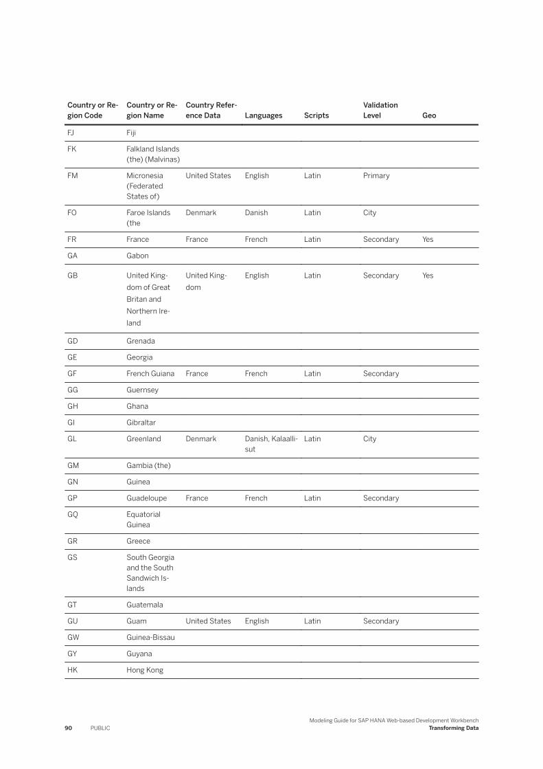
Country or Region Code
Country or Region Name
Country Reference Data Languages Scripts
Validation Level Geo
FJ Fiji
FK Falkland Islands (the) (Malvinas)
FM Micronesia (Federated States of)
United States English Latin Primary
FO Faroe Islands (the
Denmark Danish Latin City
FR France France French Latin Secondary Yes
GA Gabon
GB United Kingdom of Great Britan and Northern Ireland
United Kingdom
English Latin Secondary Yes
GD Grenada
GE Georgia
GF French Guiana France French Latin Secondary
GG Guernsey
GH Ghana
GI Gibraltar
GL Greenland Denmark Danish, Kalaallisut
Latin City
GM Gambia (the)
GN Guinea
GP Guadeloupe France French Latin Secondary
GQ Equatorial Guinea
GR Greece
GS South Georgia and the South Sandwich Islands
GT Guatemala
GU Guam United States English Latin Secondary
GW Guinea-Bissau
GY Guyana
HK Hong Kong
90 PUBLICModeling Guide for SAP HANA Web-based Development Workbench
Transforming Data
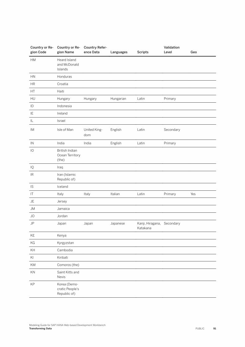
Country or Region Code
Country or Region Name
Country Reference Data Languages Scripts
Validation Level Geo
HM Heard Island and McDonald Islands
HN Honduras
HR Croatia
HT Haiti
HU Hungary Hungary Hungarian Latin Primary
ID Indonesia
IE Ireland
IL Israel
IM Isle of Man United Kingdom
English Latin Secondary
IN India India English Latin Primary
IO British Indian Ocean Territory (the)
IQ Iraq
IR Iran (Islamic Republic of)
IS Iceland
IT Italy Italy Italian Latin Primary Yes
JE Jersey
JM Jamaica
JO Jordan
JP Japan Japan Japanese Kanji, Hiragana, Katakana
Secondary
KE Kenya
KG Kyrgyzstan
KH Cambodia
KI Kiribati
KM Comoros (the)
KN Saint Kitts and Nevis
KP Korea (Democratic People's Republic of)
Modeling Guide for SAP HANA Web-based Development WorkbenchTransforming Data PUBLIC 91
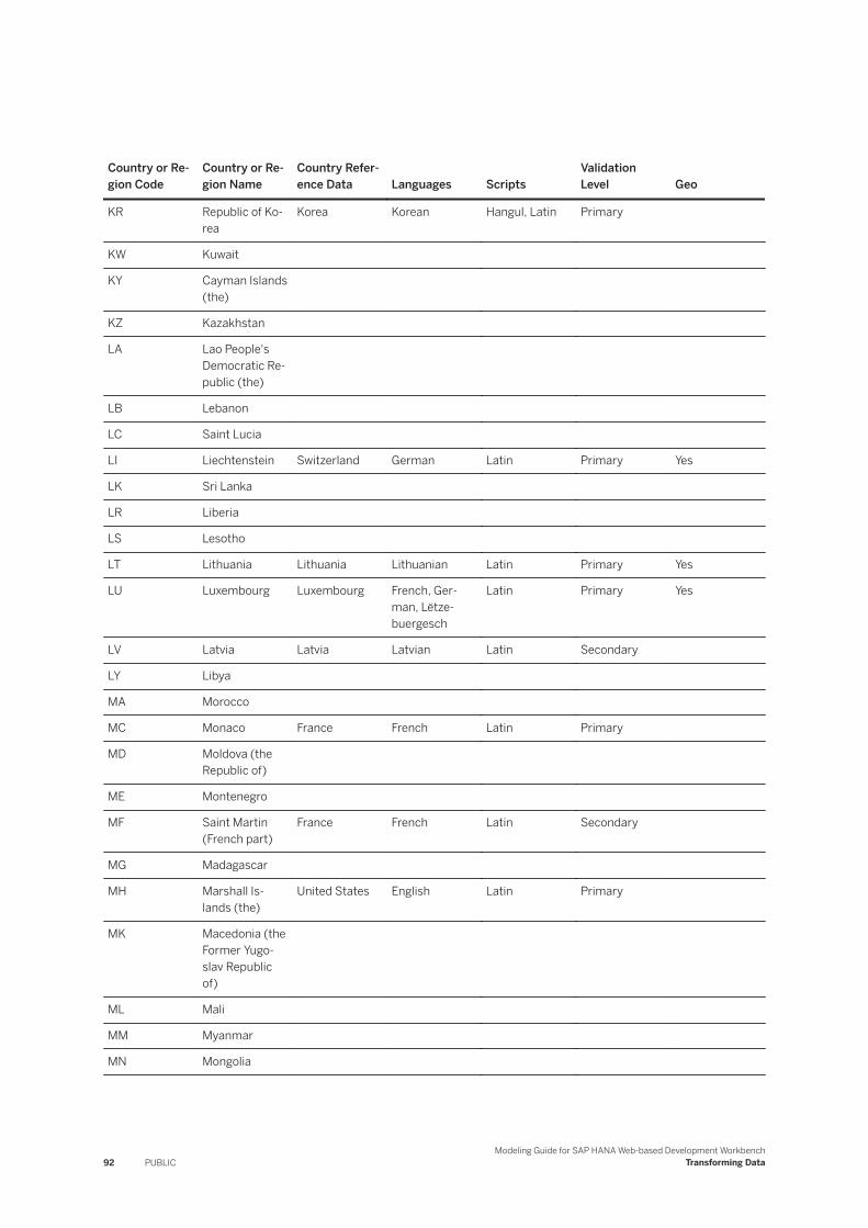
Country or Region Code
Country or Region Name
Country Reference Data Languages Scripts
Validation Level Geo
KR Republic of Korea
Korea Korean Hangul, Latin Primary
KW Kuwait
KY Cayman Islands (the)
KZ Kazakhstan
LA Lao People's Democratic Republic (the)
LB Lebanon
LC Saint Lucia
LI Liechtenstein Switzerland German Latin Primary Yes
LK Sri Lanka
LR Liberia
LS Lesotho
LT Lithuania Lithuania Lithuanian Latin Primary Yes
LU Luxembourg Luxembourg French, German, Lëtzebuergesch
Latin Primary Yes
LV Latvia Latvia Latvian Latin Secondary
LY Libya
MA Morocco
MC Monaco France French Latin Primary
MD Moldova (the Republic of)
ME Montenegro
MF Saint Martin (French part)
France French Latin Secondary
MG Madagascar
MH Marshall Islands (the)
United States English Latin Primary
MK Macedonia (the Former Yugoslav Republic of)
ML Mali
MM Myanmar
MN Mongolia
92 PUBLICModeling Guide for SAP HANA Web-based Development Workbench
Transforming Data
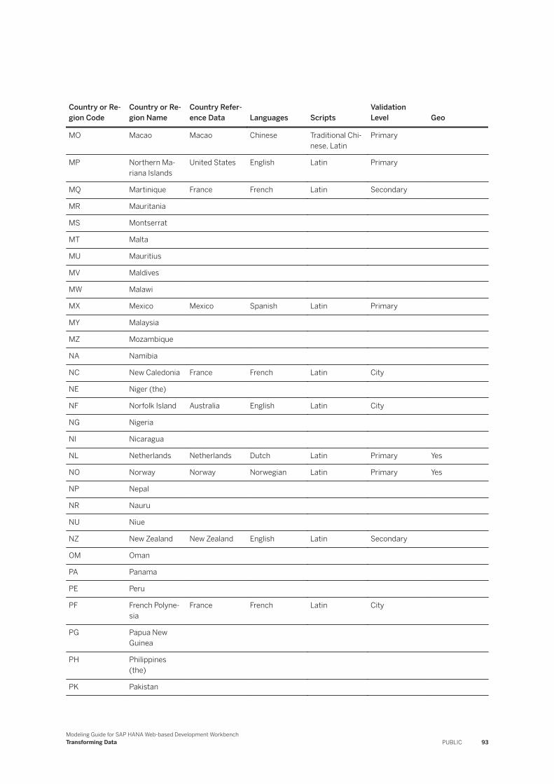
Country or Region Code
Country or Region Name
Country Reference Data Languages Scripts
Validation Level Geo
MO Macao Macao Chinese Traditional Chinese, Latin
Primary
MP Northern Mariana Islands
United States English Latin Primary
MQ Martinique France French Latin Secondary
MR Mauritania
MS Montserrat
MT Malta
MU Mauritius
MV Maldives
MW Malawi
MX Mexico Mexico Spanish Latin Primary
MY Malaysia
MZ Mozambique
NA Namibia
NC New Caledonia France French Latin City
NE Niger (the)
NF Norfolk Island Australia English Latin City
NG Nigeria
NI Nicaragua
NL Netherlands Netherlands Dutch Latin Primary Yes
NO Norway Norway Norwegian Latin Primary Yes
NP Nepal
NR Nauru
NU Niue
NZ New Zealand New Zealand English Latin Secondary
OM Oman
PA Panama
PE Peru
PF French Polynesia
France French Latin City
PG Papua New Guinea
PH Philippines (the)
PK Pakistan
Modeling Guide for SAP HANA Web-based Development WorkbenchTransforming Data PUBLIC 93

Country or Region Code
Country or Region Name
Country Reference Data Languages Scripts
Validation Level Geo
PL Poland Poland Polish Latin Primary Yes
PM Saint Pierre and Miquelon
France French Latin City
PN Pitcairn
PR Puerto Rico United States Spanish Latin Secondary
PS Palestine (State of)
PT Portugal Portugal Portuguese Latin Secondary Yes
PW Palau United States English Latin Primary
PY Paraguay
QA Qatar
RE Réunion France French Latin Secondary
RO Romania
RS Serbia
RU Russia Russia Russian Cyrillic, Latin Primary
RW Rwanda
SA Saudi Arabia
SB Solomon Islands
SC Seychelles
SD Sudan (The)
SE Sweden Sweden Swedish Latin Primary Yes
SG Singapore Singapore English Latin Primary
SH Saint Helena, Ascension, and Tristan da Cunha
SI Slovenia
SJ Svalbard and Jan Mayen
Norway Norwegian Latin Primary
SK Slovakia Slovakia Slovakian Latin Primary
SL Sierra Leone
SM San Marino Italy Italian Latin Primary
SN Senegal
SO Somalia
SR Suriname
94 PUBLICModeling Guide for SAP HANA Web-based Development Workbench
Transforming Data
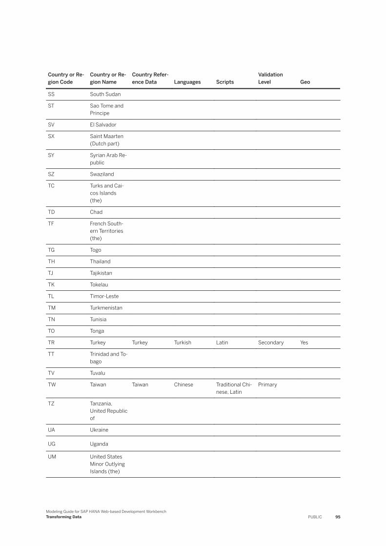
Country or Region Code
Country or Region Name
Country Reference Data Languages Scripts
Validation Level Geo
SS South Sudan
ST Sao Tome and Principe
SV El Salvador
SX Saint Maarten (Dutch part)
SY Syrian Arab Republic
SZ Swaziland
TC Turks and Caicos Islands (the)
TD Chad
TF French Southern Territories (the)
TG Togo
TH Thailand
TJ Tajikistan
TK Tokelau
TL Timor-Leste
TM Turkmenistan
TN Tunisia
TO Tonga
TR Turkey Turkey Turkish Latin Secondary Yes
TT Trinidad and Tobago
TV Tuvalu
TW Taiwan Taiwan Chinese Traditional Chinese, Latin
Primary
TZ Tanzania, United Republic of
UA Ukraine
UG Uganda
UM United States Minor Outlying Islands (the)
Modeling Guide for SAP HANA Web-based Development WorkbenchTransforming Data PUBLIC 95
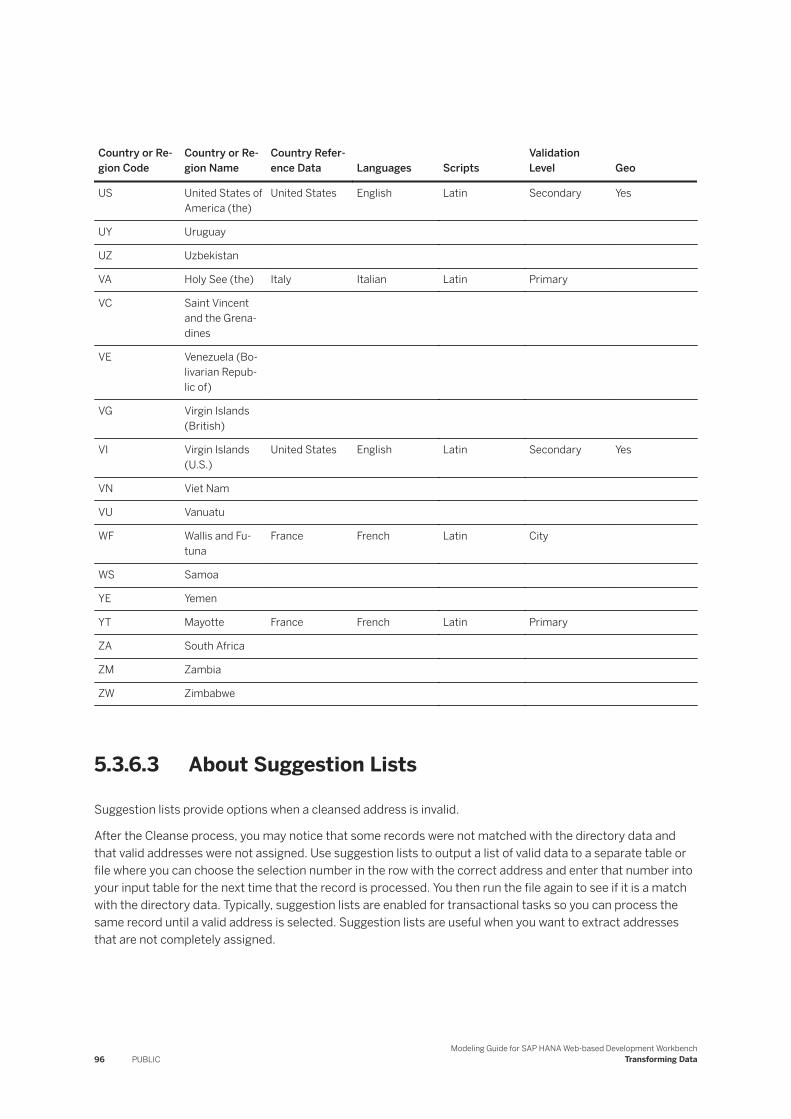
Country or Region Code
Country or Region Name
Country Reference Data Languages Scripts
Validation Level Geo
US United States of America (the)
United States English Latin Secondary Yes
UY Uruguay
UZ Uzbekistan
VA Holy See (the) Italy Italian Latin Primary
VC Saint Vincent and the Grenadines
VE Venezuela (Bolivarian Republic of)
VG Virgin Islands (British)
VI Virgin Islands (U.S.)
United States English Latin Secondary Yes
VN Viet Nam
VU Vanuatu
WF Wallis and Futuna
France French Latin City
WS Samoa
YE Yemen
YT Mayotte France French Latin Primary
ZA South Africa
ZM Zambia
ZW Zimbabwe
5.3.6.3 About Suggestion Lists
Suggestion lists provide options when a cleansed address is invalid.
After the Cleanse process, you may notice that some records were not matched with the directory data and that valid addresses were not assigned. Use suggestion lists to output a list of valid data to a separate table or file where you can choose the selection number in the row with the correct address and enter that number into your input table for the next time that the record is processed. You then run the file again to see if it is a match with the directory data. Typically, suggestion lists are enabled for transactional tasks so you can process the same record until a valid address is selected. Suggestion lists are useful when you want to extract addresses that are not completely assigned.
96 PUBLICModeling Guide for SAP HANA Web-based Development Workbench
Transforming Data

How Suggestion Lists Work
Your input file or table must contain a column, for example REPLY, so the application can identify your choice for the correct address. Then you select Enable suggestion list in the Default Cleanse Settings dialog in the Cleanse node. You need to select the column that contains the selection number of your choice, for example, the REPLY column. After configuring the Cleanse node, you route the valid addresses to one table using the Output pipe and the list of suggested addresses for those address that are invalid to a separate output table using the Suggestion_List output pipe. After reviewing the list of suggestions in the output table, you choose the associated selection number in the row with the data that you want to use to get a valid address, and then enter that number in the REPLY column in the input file record. You then run the record through Cleanse again, which uses the address you selected to see if it is valid. If it is not, the application outputs another suggestion list with a more specific location for you to choose another option.
NoteThe reply column must be a string value with an Unknown content type assignment.
The information in the suggestion list table is dependent on where the ambiguity lies in the data. The first time a suggestion list is output, it includes the broadest ambiguous data that occurs in the record. For example, if the region is ambiguous, you see region data in the suggestion list. After the record runs again, the system outputs suggestions for the next level of ambiguity. For example, if the region and locality are valid, you see address line data in the suggestion list. The application continues to output more specific suggestions each time the record is processed until a valid address is output.
For example, let's say that you have the following data in a record:
Sample Code
Raiffeisenring St. Leon-RotGermany
The first time the record is run, the application might look for the correct street for the address. You'll see a status of "A" for address.
Selection Number Option Error Status
1 RAIFFEISENRING 1-999 3 A
2 RAIFFEISENSTR 1-999 3 A
In your input table under the REPLY column for this record, you enter the selection number for the valid street. If perhaps you are looking for an address in the business district, then you would enter 1 in the REPLY column to select Raiffeisenring 1-999. Let's say that you run the address a second time, but it is still not a valid address. Because you already know the street, the address number is the next set of options to choose from the suggestion list table. You will see a status of R for range. Enter a value between 1 and 999 as indicated in the previous table.
Alternatively, because the initial suggestion included the range in the output, you could enter the address number in the previous step by using a pipe in your selection. The first number is the selection number, then you enter the pipe ( | ), followed by the number of the address. For example, you would type 1|45 in the REPLY column if the valid address is Raiffeisenring 45, 68789 St. Leon-Rot, Germany.
Modeling Guide for SAP HANA Web-based Development WorkbenchTransforming Data PUBLIC 97
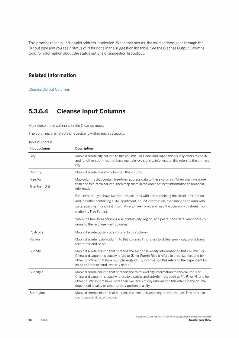
This process repeats until a valid address is selected. When that occurs, the valid address goes through the Output pipe and you see a status of N for none in the suggestion list table. See the Cleanse Output Columns topic for information about the status options of suggestion list output.
Related Information
Cleanse Output Columns
5.3.6.4 Cleanse Input Columns
Map these input columns in the Cleanse node.
The columns are listed alphabetically within each category.
Table 2: Address
Input column Description
City Map a discrete city column to this column. For China and Japan this usually refers to the 市, and for other countries that have multiple levels of city information this refers to the primary city.
Country Map a discrete country column to this column.
Free Form
Free Form 2-6
Map columns that contain free-form address data to these columns. When you have more than one free-form column, then map them in the order of finest information to broadest information.
For example, if you have two address columns with one containing the street information and the other containing suite, apartment, or unit information, then map the column with suite, apartment, and unit information to Free Form, and map the column with street information to Free Form 2.
When the free-form columns also contain city, region, and postal code data, map these columns to the last Free Form columns.
Postcode Map a discrete postal code column to this column.
Region Map a discrete region column to this column. This refers to states, provinces, prefectures, territories, and so on.
Subcity Map a discrete column that contains the second level city information to this column. For China and Japan this usually refers to 区, for Puerto Rico it refers to urbanization, and for other countries that have multiple levels of city information this refers to the dependent locality or other second level city name.
Subcity2 Map a discrete column that contains the third level city information to this column. For China and Japan this usually refers to districts and sub-districts such as 町, 镇, or 村, and for other countries that have more than two levels of city information this refers to the double dependent locality or other tertiary portion of a city.
Subregion Map a discrete column that contains the second level of region information. This refers to counties, districts, and so on.
98 PUBLICModeling Guide for SAP HANA Web-based Development Workbench
Transforming Data
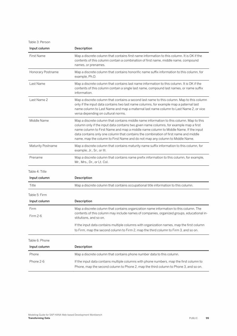
Table 3: Person
Input column Description
First Name Map a discrete column that contains first name information to this column. It is OK if the contents of this column contain a combination of first name, middle name, compound names, or prenames.
Honorary Postname Map a discrete column that contains honorific name suffix information to this column, for example, Ph.D.
Last Name Map a discrete column that contains last name information to this column. It is OK if the contents of this column contain a single last name, compound last names, or name suffix information.
Last Name 2 Map a discrete column that contains a second last name to this column. Map to this column only if the input data contains two last name columns, for example map a paternal last name column to Last Name and map a maternal last name column to Last Name 2, or vice versa depending on cultural norms.
Middle Name Map a discrete column that contains middle name information to this column. Map to this column only if the input data contains two given name columns, for example map a first name column to First Name and map a middle name column to Middle Name. If the input data contains only one column that contains the combination of first name and middle name, map the column to First Name and do not map any column to Middle Name.
Maturity Postname Map a discrete column that contains maturity name suffix information to this column, for example, Jr., Sr., or III.
Prename Map a discrete column that contains name prefix information to this column, for example, Mr., Mrs., Dr., or Lt. Col.
Table 4: Title
Input column Description
Title Map a discrete column that contains occupational title information to this column.
Table 5: Firm
Input column Description
Firm
Firm 2-6
Map a discrete column that contains organization name information to this column. The contents of this column may include names of companies, organized groups, educational institutions, and so on.
If the input data contains multiple columns with organization names, map the first column to Firm, map the second column to Firm 2, map the third column to Firm 3, and so on.
Table 6: Phone
Input column Description
Phone
Phone 2-6
Map a discrete column that contains phone number data to this column.
If the input data contains multiple columns with phone numbers, map the first column to Phone, map the second column to Phone 2, map the third column to Phone 3, and so on.
Modeling Guide for SAP HANA Web-based Development WorkbenchTransforming Data PUBLIC 99
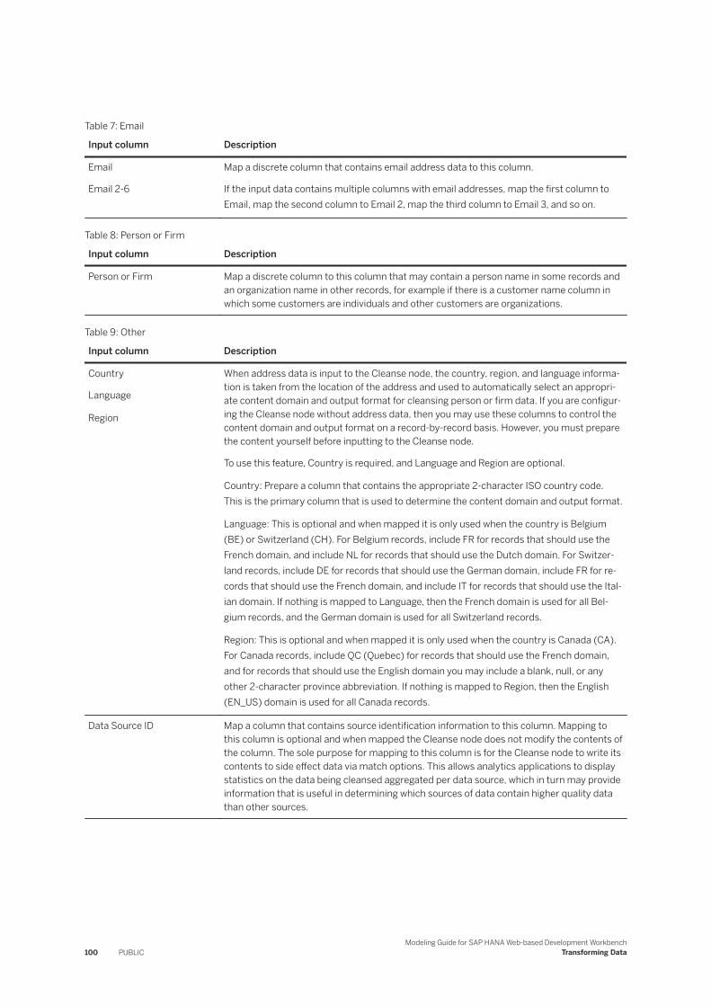
Table 7: Email
Input column Description
Email 2-6
Map a discrete column that contains email address data to this column.
If the input data contains multiple columns with email addresses, map the first column to Email, map the second column to Email 2, map the third column to Email 3, and so on.
Table 8: Person or Firm
Input column Description
Person or Firm Map a discrete column to this column that may contain a person name in some records and an organization name in other records, for example if there is a customer name column in which some customers are individuals and other customers are organizations.
Table 9: Other
Input column Description
Country
Language
Region
When address data is input to the Cleanse node, the country, region, and language information is taken from the location of the address and used to automatically select an appropriate content domain and output format for cleansing person or firm data. If you are configur-ing the Cleanse node without address data, then you may use these columns to control the content domain and output format on a record-by-record basis. However, you must prepare the content yourself before inputting to the Cleanse node.
To use this feature, Country is required, and Language and Region are optional.
Country: Prepare a column that contains the appropriate 2-character ISO country code. This is the primary column that is used to determine the content domain and output format.
Language: This is optional and when mapped it is only used when the country is Belgium (BE) or Switzerland (CH). For Belgium records, include FR for records that should use the French domain, and include NL for records that should use the Dutch domain. For Switzerland records, include DE for records that should use the German domain, include FR for records that should use the French domain, and include IT for records that should use the Italian domain. If nothing is mapped to Language, then the French domain is used for all Belgium records, and the German domain is used for all Switzerland records.
Region: This is optional and when mapped it is only used when the country is Canada (CA). For Canada records, include QC (Quebec) for records that should use the French domain, and for records that should use the English domain you may include a blank, null, or any other 2-character province abbreviation. If nothing is mapped to Region, then the English (EN_US) domain is used for all Canada records.
Data Source ID Map a column that contains source identification information to this column. Mapping to this column is optional and when mapped the Cleanse node does not modify the contents of the column. The sole purpose for mapping to this column is for the Cleanse node to write its contents to side effect data via match options. This allows analytics applications to display statistics on the data being cleansed aggregated per data source, which in turn may provide information that is useful in determining which sources of data contain higher quality data than other sources.
100 PUBLICModeling Guide for SAP HANA Web-based Development Workbench
Transforming Data
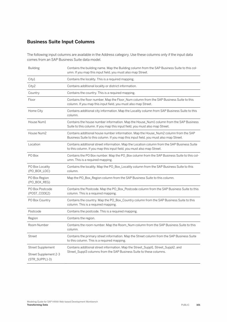
Business Suite Input Columns
The following input columns are available in the Address category. Use these columns only if the input data comes from an SAP Business Suite data model.
Building Contains the building name. Map the Building column from the SAP Business Suite to this column. If you map this input field, you must also map Street.
City1 Contains the locality. This is a required mapping.
City2 Contains additional locality or district information.
Country Contains the country. This is a required mapping.
Floor Contains the floor number. Map the Floor_Num column from the SAP Business Suite to this column. If you map this input field, you must also map Street.
Home City Contains additional city information. Map the Locality column from SAP Business Suite to this column.
House Num1 Contains the house number information. Map the House_Num1 column from the SAP Business Suite to this column. If you map this input field, you must also map Street.
House Num2 Contains additional house number information. Map the House_Num2 column from the SAP Business Suite to this column. If you map this input field, you must also map Street.
Location Contains additional street information. Map the Location column from the SAP Business Suite to this column. If you map this input field, you must also map Street.
PO Box Contains the PO Box number. Map the PO_Box column from the SAP Business Suite to this column. This is a required mapping.
PO Box Locality (PO_BOX_LOC)
Contains the locality. Map the PO_Box_Locality column from the SAP Business Suite to this column.
PO Box Region (PO_BOX_REG)
Map the PO_Box_Region column from the SAP Business Suite to this column.
PO Box Postcode (POST_CODE2)
Contains the Postcode. Map the PO_Box_Postcode column from the SAP Business Suite to this column. This is a required mapping.
PO Box Country Contains the country. Map the PO_Box_Country column from the SAP Business Suite to this column. This is a required mapping.
Postcode Contains the postcode. This is a required mapping.
Region Contains the region.
Room Number Contains the room number. Map the Room_Num column from the SAP Business Suite to this column.
Street Contains the primary street information. Map the Street column from the SAP Business Suite to this column. This is a required mapping.
Street Supplement
Street Supplement 2-3 (STR_SUPPL1-3)
Contains additional street information. Map the Street_Suppl1, Street_Suppl2, and Street_Suppl3 columns from the SAP Business Suite to these columns.
Modeling Guide for SAP HANA Web-based Development WorkbenchTransforming Data PUBLIC 101

Suggestion List Input Columns
The following input column is available in the Address category.
Input column Description
Suggestion Reply Contains the reply when more information is needed to complete the query. Each of these columns also contains the reply if a selection from a list needs to be made. Possible types of generated suggestion lists are:
● Lastline● Primary Address● Follow-up Primary Address● Secondary Address● Follow-up Secondary Address
Related Information
Match Options
5.3.6.5 Cleanse Output Columns
List of the output columns available in the Cleanse node.
The following are output columns that contain cleansed data. The columns are listed alphabetically within each category. The information codes related to these output columns are also listed.
NoteThe Output Column Name is the one you select when mapping columns. The Generated Output Column Name is the name of the column shown in the target table.
Table 10: Address Basic
Output and Generated Output Column Name Description
Address
STD_ADDR_ADDRESS_DELIVERY
The combination of Street Address and Secondary Address, for example in “100 Main St Apt 201, PO Box 500, Chicago IL 60612-8157” the Address is “100 Main St Apt 201”.
Building Name
STD_ADDR_BUILDING_NAME
The name of the building, for example “Opera House” or “Empire Tower”.
City
STD_ADDR_LOCALITY
The city name, for example “Paris” or “上海”. If you wish the city name to include the qualifier or descriptor then you should select City (Expanded) instead.
102 PUBLICModeling Guide for SAP HANA Web-based Development Workbench
Transforming Data

Output and Generated Output Column Name Description
City (Expanded)
STD_ADDR_LOCALITY_FULL
Includes City, City Code, City Description, and City Qualifier, for example in Germany the City is "Frankfurt". City (Expanded) is "Frankfurt am Main". In Japan City is "墨田". City (Expanded) is "墨田区".
Country
STD_ADDR_COUNTRY_NAME
The country name fully spelled out in English, for example “Germany”.
Country Code
STD_ADDR_COUNTRY_2CHAR
The 2-character ISO country code, for example “DE” for Germany.
Dual Address
STD_ADDR_ADDRESS_DUAL
The second address when the input address contains two addresses sharing the same city, region, and postcode. For example, in “100 Main St Apt 201, PO Box 500, Chicago IL 60612-8157”, the dual address is “PO Box 500”.
Postcode
STD_ADDR_POSTCODE_FULL
The full postal code, for example “60612-8157” in the United States, “102-8539” in Japan, and “RG17 1JF” in the United Kingdom.
Postcode 1
STD_ADDR_POSTCODE1
For countries that have two parts to their postal codes, Postcode 1 contains the first part. For example, for the United States postal code “60612-8157” the Postcode 1 is “60612”. For all other countries, Postcode 1 contains the full postal code. For example, for the Germany postal code “12610” the Postcode 1 is “12610”.
Postcode 2
STD_ADDR_POSTCODE2
For countries that have two parts to their postal codes, Postcode 2 contains the second part. For example, for the United States postal code “60612-8157” the Postcode 2 is “8157”. For all other countries, Postcode 2 is empty. For example, for the Germany postal code “12610” the Postcode 2 is empty.
Region
STD_ADDR_REGION
The region name, either abbreviated or fully spelled out based on the Region Formatting setting, for example “California” or “上海”. If you want the region name to include the descriptor, then you should select Region (Expanded) instead.
Region (Expanded)
STD_ADDR_REGION_FULL
The region name with the descriptor, for example “上海市” instead of “上海”.
Secondary Address
STD_ADDR_SEC_ADDRESS
The interior portion of the address. For example, in “100 Main St Apt 201, PO Box 500, Chicago IL 60612-8157” the Secondary Address is “Apt 201”.
Street Address
STD_ADDR_PRIM_ADDRESS
The exterior portion of the address. For example, in “100 Main St Apt 201, PO Box 500, Chicago IL 60612-8157” the Street Address is “100 Main St”.
Subcity
STD_ADDR_LOCALITY2
Name of the second level of city information, for example in “中央区” the Subcity is “中央”. For China and Japan this usually refers to 区, for Puerto Rico it refers to urbanization, and for other countries that have multiple levels of city information this refers to the dependent locality or other secondary portion of a city. If you want the subcity name to include the descriptor, then you should select Subcity (Expanded) instead.
Subcity (Expanded)
STD_ADDR_LOCALITY2_FULL
Second level of city information with the descriptor, for example “中央区” instead of “中央”. For China and Japan this usually refers to 区, for Puerto Rico it refers to urbanization, and for other countries that have multiple levels of city information this refers to the dependent locality or other secondary portion of a city.
Modeling Guide for SAP HANA Web-based Development WorkbenchTransforming Data PUBLIC 103
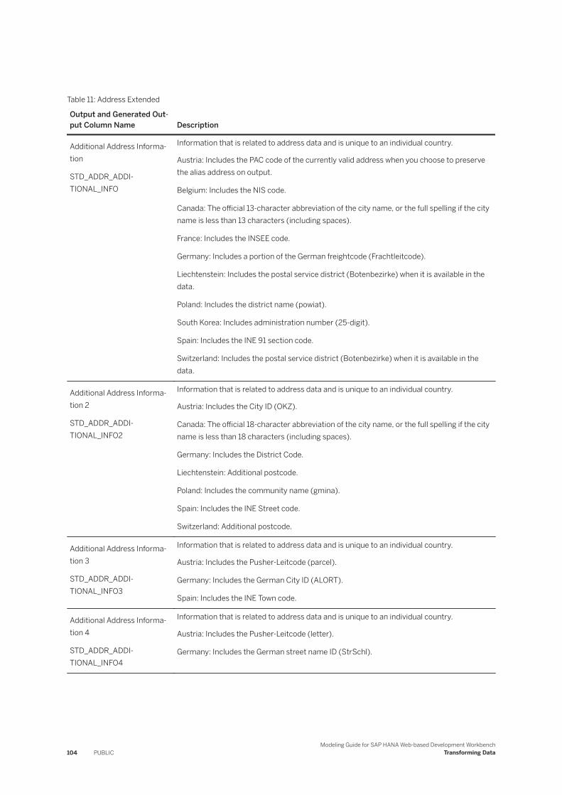
Table 11: Address Extended
Output and Generated Output Column Name Description
Additional Address Information
STD_ADDR_ADDITIONAL_INFO
Information that is related to address data and is unique to an individual country.
Austria: Includes the PAC code of the currently valid address when you choose to preserve the alias address on output.
Belgium: Includes the NIS code.
Canada: The official 13-character abbreviation of the city name, or the full spelling if the city name is less than 13 characters (including spaces).
France: Includes the INSEE code.
Germany: Includes a portion of the German freightcode (Frachtleitcode).
Liechtenstein: Includes the postal service district (Botenbezirke) when it is available in the data.
Poland: Includes the district name (powiat).
South Korea: Includes administration number (25-digit).
Spain: Includes the INE 91 section code.
Switzerland: Includes the postal service district (Botenbezirke) when it is available in the data.
Additional Address Information 2
STD_ADDR_ADDITIONAL_INFO2
Information that is related to address data and is unique to an individual country.
Austria: Includes the City ID (OKZ).
Canada: The official 18-character abbreviation of the city name, or the full spelling if the city name is less than 18 characters (including spaces).
Germany: Includes the District Code.
Liechtenstein: Additional postcode.
Poland: Includes the community name (gmina).
Spain: Includes the INE Street code.
Switzerland: Additional postcode.
Additional Address Information 3
STD_ADDR_ADDITIONAL_INFO3
Information that is related to address data and is unique to an individual country.
Austria: Includes the Pusher-Leitcode (parcel).
Germany: Includes the German City ID (ALORT).
Spain: Includes the INE Town code.
Additional Address Information 4
STD_ADDR_ADDITIONAL_INFO4
Information that is related to address data and is unique to an individual country.
Austria: Includes the Pusher-Leitcode (letter).
Germany: Includes the German street name ID (StrSchl).
104 PUBLICModeling Guide for SAP HANA Web-based Development Workbench
Transforming Data
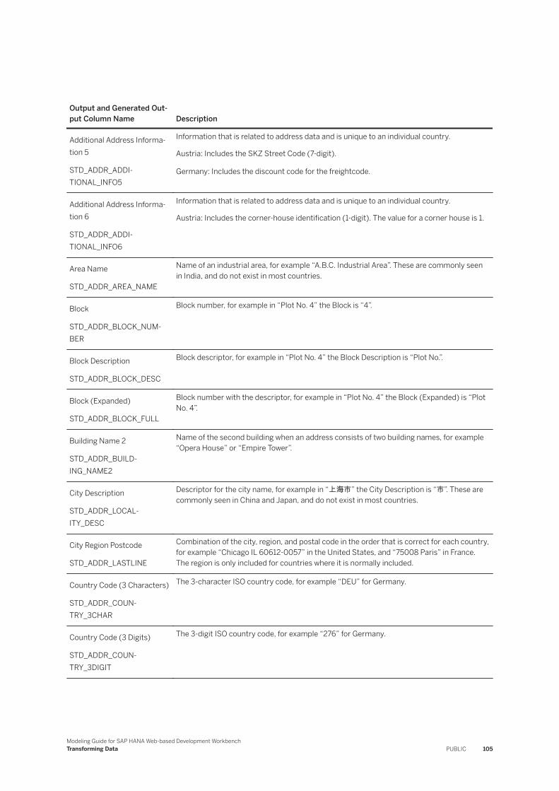
Output and Generated Output Column Name Description
Additional Address Information 5
STD_ADDR_ADDITIONAL_INFO5
Information that is related to address data and is unique to an individual country.
Austria: Includes the SKZ Street Code (7-digit).
Germany: Includes the discount code for the freightcode.
Additional Address Information 6
STD_ADDR_ADDITIONAL_INFO6
Information that is related to address data and is unique to an individual country.
Austria: Includes the corner-house identification (1-digit). The value for a corner house is 1.
Area Name
STD_ADDR_AREA_NAME
Name of an industrial area, for example “A.B.C. Industrial Area”. These are commonly seen in India, and do not exist in most countries.
Block
STD_ADDR_BLOCK_NUMBER
Block number, for example in “Plot No. 4” the Block is “4”.
Block Description
STD_ADDR_BLOCK_DESC
Block descriptor, for example in “Plot No. 4” the Block Description is “Plot No.”.
Block (Expanded)
STD_ADDR_BLOCK_FULL
Block number with the descriptor, for example in “Plot No. 4” the Block (Expanded) is “Plot No. 4”.
Building Name 2
STD_ADDR_BUILDING_NAME2
Name of the second building when an address consists of two building names, for example “Opera House” or “Empire Tower”.
City Description
STD_ADDR_LOCALITY_DESC
Descriptor for the city name, for example in “上海市” the City Description is “市”. These are commonly seen in China and Japan, and do not exist in most countries.
City Region Postcode
STD_ADDR_LASTLINE
Combination of the city, region, and postal code in the order that is correct for each country, for example “Chicago IL 60612-0057” in the United States, and “75008 Paris” in France. The region is only included for countries where it is normally included.
Country Code (3 Characters)
STD_ADDR_COUNTRY_3CHAR
The 3-character ISO country code, for example “DEU” for Germany.
Country Code (3 Digits)
STD_ADDR_COUNTRY_3DIGIT
The 3-digit ISO country code, for example “276” for Germany.
Modeling Guide for SAP HANA Web-based Development WorkbenchTransforming Data PUBLIC 105
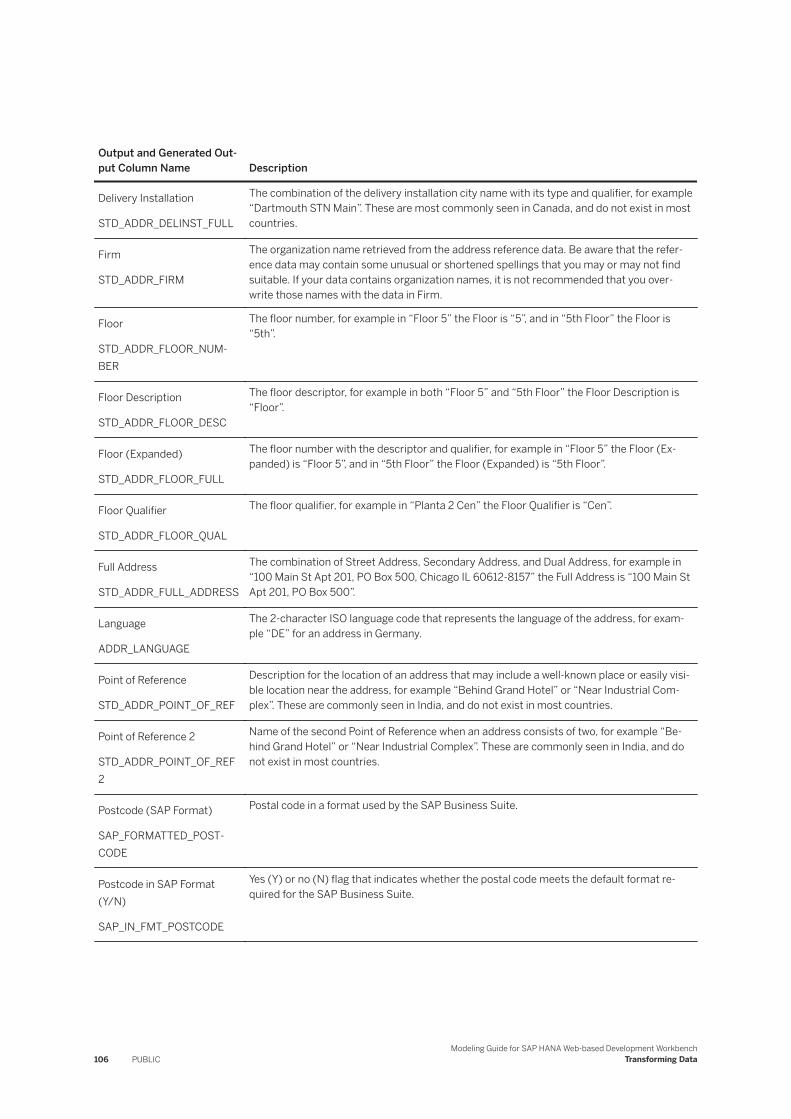
Output and Generated Output Column Name Description
Delivery Installation
STD_ADDR_DELINST_FULL
The combination of the delivery installation city name with its type and qualifier, for example “Dartmouth STN Main”. These are most commonly seen in Canada, and do not exist in most countries.
Firm
STD_ADDR_FIRM
The organization name retrieved from the address reference data. Be aware that the reference data may contain some unusual or shortened spellings that you may or may not find suitable. If your data contains organization names, it is not recommended that you overwrite those names with the data in Firm.
Floor
STD_ADDR_FLOOR_NUMBER
The floor number, for example in “Floor 5” the Floor is “5”, and in “5th Floor” the Floor is “5th”.
Floor Description
STD_ADDR_FLOOR_DESC
The floor descriptor, for example in both “Floor 5” and “5th Floor” the Floor Description is “Floor”.
Floor (Expanded)
STD_ADDR_FLOOR_FULL
The floor number with the descriptor and qualifier, for example in “Floor 5” the Floor (Expanded) is “Floor 5”, and in “5th Floor” the Floor (Expanded) is “5th Floor”.
Floor Qualifier
STD_ADDR_FLOOR_QUAL
The floor qualifier, for example in “Planta 2 Cen” the Floor Qualifier is “Cen”.
Full Address
STD_ADDR_FULL_ADDRESS
The combination of Street Address, Secondary Address, and Dual Address, for example in “100 Main St Apt 201, PO Box 500, Chicago IL 60612-8157” the Full Address is “100 Main St Apt 201, PO Box 500”.
Language
ADDR_LANGUAGE
The 2-character ISO language code that represents the language of the address, for example “DE” for an address in Germany.
Point of Reference
STD_ADDR_POINT_OF_REF
Description for the location of an address that may include a well-known place or easily visible location near the address, for example “Behind Grand Hotel” or “Near Industrial Complex”. These are commonly seen in India, and do not exist in most countries.
Point of Reference 2
STD_ADDR_POINT_OF_REF2
Name of the second Point of Reference when an address consists of two, for example “Behind Grand Hotel” or “Near Industrial Complex”. These are commonly seen in India, and do not exist in most countries.
Postcode (SAP Format)
SAP_FORMATTED_POSTCODE
Postal code in a format used by the SAP Business Suite.
Postcode in SAP Format (Y/N)
SAP_IN_FMT_POSTCODE
Yes (Y) or no (N) flag that indicates whether the postal code meets the default format required for the SAP Business Suite.
106 PUBLICModeling Guide for SAP HANA Web-based Development Workbench
Transforming Data
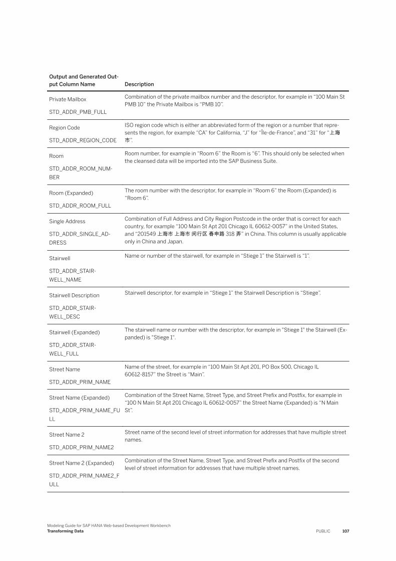
Output and Generated Output Column Name Description
Private Mailbox
STD_ADDR_PMB_FULL
Combination of the private mailbox number and the descriptor, for example in “100 Main St PMB 10” the Private Mailbox is “PMB 10”.
Region Code
STD_ADDR_REGION_CODE
ISO region code which is either an abbreviated form of the region or a number that represents the region, for example “CA” for California, “J” for “Île-de-France”, and “31” for “上海市”.
Room
STD_ADDR_ROOM_NUMBER
Room number, for example in “Room 6” the Room is “6”. This should only be selected when the cleansed data will be imported into the SAP Business Suite.
Room (Expanded)
STD_ADDR_ROOM_FULL
The room number with the descriptor, for example in “Room 6” the Room (Expanded) is “Room 6”.
Single Address
STD_ADDR_SINGLE_ADDRESS
Combination of Full Address and City Region Postcode in the order that is correct for each country, for example “100 Main St Apt 201 Chicago IL 60612-0057” in the United States, and “201549 上海市 上海市 闵行区 春申路 318 弄” in China. This column is usually applicable only in China and Japan.
Stairwell
STD_ADDR_STAIRWELL_NAME
Name or number of the stairwell, for example in “Stiege 1” the Stairwell is “1”.
Stairwell Description
STD_ADDR_STAIRWELL_DESC
Stairwell descriptor, for example in “Stiege 1” the Stairwell Description is “Stiege”.
Stairwell (Expanded)
STD_ADDR_STAIRWELL_FULL
The stairwell name or number with the descriptor, for example in "Stiege 1" the Stairwell (Expanded) is "Stiege 1".
Street Name
STD_ADDR_PRIM_NAME
Name of the street, for example in “100 Main St Apt 201, PO Box 500, Chicago IL 60612-8157” the Street is “Main”.
Street Name (Expanded)
STD_ADDR_PRIM_NAME_FULL
Combination of the Street Name, Street Type, and Street Prefix and Postfix, for example in “100 N Main St Apt 201 Chicago IL 60612-0057” the Street Name (Expanded) is “N Main St”.
Street Name 2
STD_ADDR_PRIM_NAME2
Street name of the second level of street information for addresses that have multiple street names.
Street Name 2 (Expanded)
STD_ADDR_PRIM_NAME2_FULL
Combination of the Street Name, Street Type, and Street Prefix and Postfix of the second level of street information for addresses that have multiple street names.
Modeling Guide for SAP HANA Web-based Development WorkbenchTransforming Data PUBLIC 107
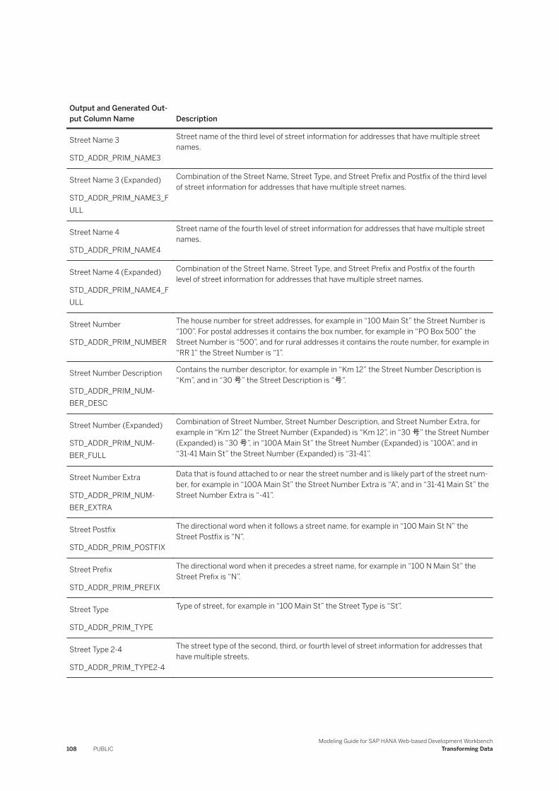
Output and Generated Output Column Name Description
Street Name 3
STD_ADDR_PRIM_NAME3
Street name of the third level of street information for addresses that have multiple street names.
Street Name 3 (Expanded)
STD_ADDR_PRIM_NAME3_FULL
Combination of the Street Name, Street Type, and Street Prefix and Postfix of the third level of street information for addresses that have multiple street names.
Street Name 4
STD_ADDR_PRIM_NAME4
Street name of the fourth level of street information for addresses that have multiple street names.
Street Name 4 (Expanded)
STD_ADDR_PRIM_NAME4_FULL
Combination of the Street Name, Street Type, and Street Prefix and Postfix of the fourth level of street information for addresses that have multiple street names.
Street Number
STD_ADDR_PRIM_NUMBER
The house number for street addresses, for example in “100 Main St” the Street Number is “100”. For postal addresses it contains the box number, for example in “PO Box 500” the Street Number is “500”, and for rural addresses it contains the route number, for example in “RR 1” the Street Number is “1”.
Street Number Description
STD_ADDR_PRIM_NUMBER_DESC
Contains the number descriptor, for example in “Km 12” the Street Number Description is “Km”, and in “30 号” the Street Description is “号”.
Street Number (Expanded)
STD_ADDR_PRIM_NUMBER_FULL
Combination of Street Number, Street Number Description, and Street Number Extra, for example in “Km 12” the Street Number (Expanded) is “Km 12”, in “30 号” the Street Number (Expanded) is “30 号”, in “100A Main St” the Street Number (Expanded) is “100A”, and in “31-41 Main St” the Street Number (Expanded) is “31-41”.
Street Number Extra
STD_ADDR_PRIM_NUMBER_EXTRA
Data that is found attached to or near the street number and is likely part of the street number, for example in “100A Main St” the Street Number Extra is “A”, and in “31-41 Main St” the Street Number Extra is “-41”.
Street Postfix
STD_ADDR_PRIM_POSTFIX
The directional word when it follows a street name, for example in “100 Main St N” the Street Postfix is “N”.
Street Prefix
STD_ADDR_PRIM_PREFIX
The directional word when it precedes a street name, for example in “100 N Main St” the Street Prefix is “N”.
Street Type
STD_ADDR_PRIM_TYPE
Type of street, for example in “100 Main St” the Street Type is “St”.
Street Type 2-4
STD_ADDR_PRIM_TYPE2-4
The street type of the second, third, or fourth level of street information for addresses that have multiple streets.
108 PUBLICModeling Guide for SAP HANA Web-based Development Workbench
Transforming Data

Output and Generated Output Column Name Description
Subcity Description
STD_ADDR_LOCALITY2_DESC
The descriptor for the second level of city information, for example in “中央区” the City Description is “区”, and in “Col Federal” the Subcity Description is “Col”.
Subcity 2
STD_ADDR_LOCALITY3
Name of the third level of city information, for example, in “岡町” the Subcity 2 is “岡”.. For China and Japan this usually refers to districts and sub-districts such as 町, 镇, or 村, and in most other countries this level of city information does not exist.
Subcity 2 Description
STD_ADDR_LOCALITY3_DESC
Descriptor for the third level of city information, for example in “岡町” the Subcity 2 Description is “町”.
Subcity 2 (Expanded)
STD_ADDR_LOCALITY3_FULL
Third level of city information with the descriptor, for example “岡町” instead of “岡”.
Subcity 3
STD_ADDR_LOCALITY4
Name of the fourth level of city information, for example in “赤岗村” the Subcity 3 is “赤岗”. Some addresses in China and Japan have this fourth level of city information, and in most other countries it does not exist.
Subcity 3 Description
STD_ADDR_LOCALITY4_DESC
Descriptor for the fourth level of city information, for example in “赤岗村” the Subcity 3 Description is “村”.
Subcity 3 (Expanded)
STD_ADDR_LOCALITY4_FULL
Fourth level of city information with the descriptor, for example “赤岗村” instead of “赤岗”.
Subregion
STD_ADDR_REGION2
Second level of region information such as county or district.
Subregion Code
STD_ADDR_REGION_CODE
Code that represents the subregion.
Unit
STD_ADDR_UNIT_NUMBER
Unit number, for example in “100 Main St Apt 201” the Unit is “201”.
Unit Description
STD_ADDR_UNIT_DESC
Unit descriptor, for example in “100 Main St Apt 201” the Unit Description is “Apt”.
Unit (Expanded)
STD_ADDR_UNIT_FULL
Unit number with the descriptor and qualifier, for example in “100 Main St Apt 201” the Unit (Expanded) is “Apt 201”.
Modeling Guide for SAP HANA Web-based Development WorkbenchTransforming Data PUBLIC 109

Output and Generated Output Column Name Description
Unit Qualifier
STD_ADDR_UNIT_QUAL
Unit qualifier, for example in “Oficina 2 D” the Unit Qualifier is “D”
Wing
STD_ADDR_WING_NAME
Wing name, for example in “Wing A” the Wing is “A”.
Wing Description
STD_ADDR_WING_DESC
Wing descriptor, for example in “Wing A” the Wing Description is “Wing”.
Wing (Expanded)
STD_ADDR_WING_FULL
Wing name with the descriptor, for example in “Wing A” the Wing (Expanded) is “Wing A”.
Table 12: Address Composite
Output and Generated Output Column Name Description
Address and Dual Address
STD_ADDR_ADDR_DELDUAL
Combination of the contents of the Address column and the contents of the Dual Address column, with the combined information in the order that is appropriate for the country, for example in “100 Main St Apt 201, PO Box 500, Chicago IL 60612-8157” the Address and Dual Address is “100 Main St Apt 201 PO Box 500”.
Address and Dual Address with Building Name
STD_ADDR_PRIMADDR_DELDUAL_BLDG
Combination of the contents of the Address column, the contents of the Dual Address column, and the contents of the Building Name column, with the combined information in the order that is appropriate for the country, for example in “Opera House, 100 Main St Apt 201, PO Box 500, Chicago IL 60612-8157” the Address and Dual Address with Building Name is “Opera House 100 Main St Apt 201 PO Box 500”.
Building Name 1-2
STD_ADDR_BUILDING_NAME1_2
Combination of the contents of the Building Name column and the contents of the Building Name 2 column.
City and Subcity
STD_ADDR_LOCALITY1_2
Combination of the contents of the City column and the contents of the Subcity column, with the two levels of city information in the order that is appropriate for the country.
City and Subcity (Expanded)
STD_ADDR_LOCALITY1_2_FULL
Combination of the contents of the City (Expanded) column and the contents of the Subcity (Expanded) column, with the two levels of city information in the order that is appropriate for the country.
City and Subcity 1-3
STD_ADDR_LOCALITY1_4
Combination of the contents of the City column, the contents of the Subcity column, the contents of the Subcity 2 column, and the contents of the Subcity 3 column, with the four levels of city information in the order that is appropriate for the country.
City and Subcity 1-3 (Expanded)
STD_ADDR_LOCALITY1_4_FULL
Combination of the contents of the City (Expanded) column, the contents of the Subcity (Expanded) column, the contents of the Subcity 2 (Expanded) column, and the contents of the Subcity 3 (Expanded) column, with the four levels of city information in the order that is appropriate for the country.
110 PUBLICModeling Guide for SAP HANA Web-based Development Workbench
Transforming Data

Output and Generated Output Column Name Description
Point of Reference 1-2
STD_ADDR_POINT_OF_REF1_2
Combination of the contents of the Point of Reference column and the contents of the Point of Reference 2 column.
Region and Subregion
STD_ADDR_REGION1_2
Combination of the contents of the Region column and the contents of the Subregion column, with the two levels of region information in the order that is appropriate for the country
Region and Subregion (Expanded)
STD_ADDR_REGION1_2_FULL
Combination of the contents of the Region (Expanded) column and the contents of the Subregion (Expanded) column, with the two levels of region information in the order that is appropriate for the country.
Secondary Address without Floor
STD_ADDR_SECADDR_NO_FLOOR
Contents of the Secondary Address column without floor information, for example in “Wing A Floor 5 Room 501” the Secondary Address without Floor is “Wing A Room 501”.
Secondary Address without Floor or Room
STD_ADDR_SECADDR_NO_FLOOR_ROOM
Contents of the Secondary Address column without floor or room information, for example in “Wing A Floor 5 Room 501” the Secondary Address without Floor or Room is “Wing A”.
Secondary Address without Room
STD_ADDR_SECADDR_NO_ROOM
Contents of the Secondary Address column without room information, for example in “Wing A Floor 5 Room 501” the Secondary Address without Room is “Wing A Floor 5”.
Street Address and Dual Address
STD_ADDR_PRIMADDR_DELDUAL
Combination of the contents of the Street Address column and the contents of the Dual Address column, with the combined information in the order that is appropriate for the country, for example in “100 Main St Apt 201, PO Box 500, Chicago IL 60612-8157” the Street Address and Dual Address is “100 Main St PO Box 500”.
Street Address and Dual Address with Building Name
STD_ADDR_ADDR_DELDUAL_BLDG
Combination of the contents of the Street Address column, the contents of the Dual Address column, and the contents of the Building Name column, with the combined information in the order that is appropriate for the country, for example in “Opera House, 100 Main St Apt 201, PO Box 500, Chicago IL 60612-8157” the Street Address and Dual Address with Building Name is “Opera House 100 Main St PO Box 500”.
Street Name 1-2
STD_ADDR_PRIM_NAME1_2
Combination of the contents of the Street Name (Expanded) column and the contents of the Street Name 2 (Expanded) column, with the two levels of street information in the order that is appropriate for the country.
Street Name 3-4
STD_ADDR_PRIM_NAME3_4
Combination of the contents of the Street Name 3 (Expanded) column and the contents of the Street Name 4 (Expanded) column, with the two levels of street information in the order that is appropriate for the country
Modeling Guide for SAP HANA Web-based Development WorkbenchTransforming Data PUBLIC 111
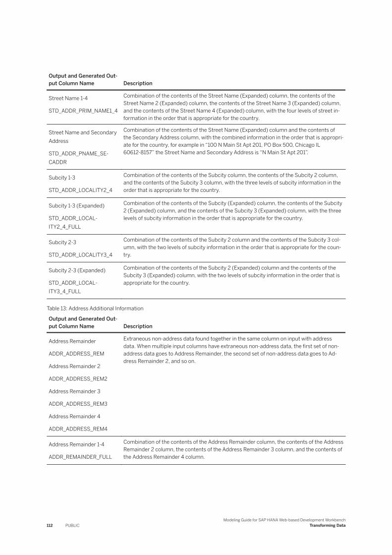
Output and Generated Output Column Name Description
Street Name 1-4
STD_ADDR_PRIM_NAME1_4
Combination of the contents of the Street Name (Expanded) column, the contents of the Street Name 2 (Expanded) column, the contents of the Street Name 3 (Expanded) column, and the contents of the Street Name 4 (Expanded) column, with the four levels of street information in the order that is appropriate for the country.
Street Name and Secondary Address
STD_ADDR_PNAME_SECADDR
Combination of the contents of the Street Name (Expanded) column and the contents of the Secondary Address column, with the combined information in the order that is appropriate for the country, for example in “100 N Main St Apt 201, PO Box 500, Chicago IL 60612-8157” the Street Name and Secondary Address is “N Main St Apt 201”.
Subcity 1-3
STD_ADDR_LOCALITY2_4
Combination of the contents of the Subcity column, the contents of the Subcity 2 column, and the contents of the Subcity 3 column, with the three levels of subcity information in the order that is appropriate for the country.
Subcity 1-3 (Expanded)
STD_ADDR_LOCALITY2_4_FULL
Combination of the contents of the Subcity (Expanded) column, the contents of the Subcity 2 (Expanded) column, and the contents of the Subcity 3 (Expanded) column, with the three levels of subcity information in the order that is appropriate for the country.
Subcity 2-3
STD_ADDR_LOCALITY3_4
Combination of the contents of the Subcity 2 column and the contents of the Subcity 3 column, with the two levels of subcity information in the order that is appropriate for the country.
Subcity 2-3 (Expanded)
STD_ADDR_LOCALITY3_4_FULL
Combination of the contents of the Subcity 2 (Expanded) column and the contents of the Subcity 3 (Expanded) column, with the two levels of subcity information in the order that is appropriate for the country.
Table 13: Address Additional Information
Output and Generated Output Column Name Description
Address Remainder
ADDR_ADDRESS_REM
Address Remainder 2
ADDR_ADDRESS_REM2
Address Remainder 3
ADDR_ADDRESS_REM3
Address Remainder 4
ADDR_ADDRESS_REM4
Extraneous non-address data found together in the same column on input with address data. When multiple input columns have extraneous non-address data, the first set of non-address data goes to Address Remainder, the second set of non-address data goes to Address Remainder 2, and so on.
Address Remainder 1-4
ADDR_REMAINDER_FULL
Combination of the contents of the Address Remainder column, the contents of the Address Remainder 2 column, the contents of the Address Remainder 3 column, and the contents of the Address Remainder 4 column.
112 PUBLICModeling Guide for SAP HANA Web-based Development Workbench
Transforming Data

Output and Generated Output Column Name Description
Address Extra
ADDR_EXTRA
Address Extra 2
ADDR_EXTRA2
Address Extra 3
ADDR_EXTRA3
Address Extra 4
ADDR_EXTRA4
Extraneous non-address data found in a column that does not have any address data. When there are multiple input columns that consist exclusively of non-address data goes to Address Extra, the second set of non-address data goes to Address Extra 2, and so on.
Address Remainder 1-4 and Address Extra 1-4
ADDR_REMAINDER_EXTRA_PMB_FULL
The combination of the contents of the Address Remainder 1-4 column, the contents of the Address Extra column, the contents of the Address Extra 2 column, the contents of the Address Extra 3 column, the contents of the Address Extra 4 column, and the contents of the Private Mail Box column.
Table 14: Address Cleanse Information
Output and Generated Output Column Name Description
Address Assignment Information
ADDR_ASMT_INFO
Information about the validity of the address. This code is also written to the ASSIGNMENT_INFORMATION column of the CLEANSE_ADDRESS_RECORD_INFO_ table in the side effect data.
C (Corrected): The input address was corrected by the Cleanse node. The cleansed address may be considered to be valid.
I (Invalid): The input address could not be validated by the Cleanse node. The cleansed address should be considered to be invalid.
V (Valid): The input address was valid and no changes or only minor changes were made by the Cleanse node. The cleansed address may be considered to be valid.
Modeling Guide for SAP HANA Web-based Development WorkbenchTransforming Data PUBLIC 113
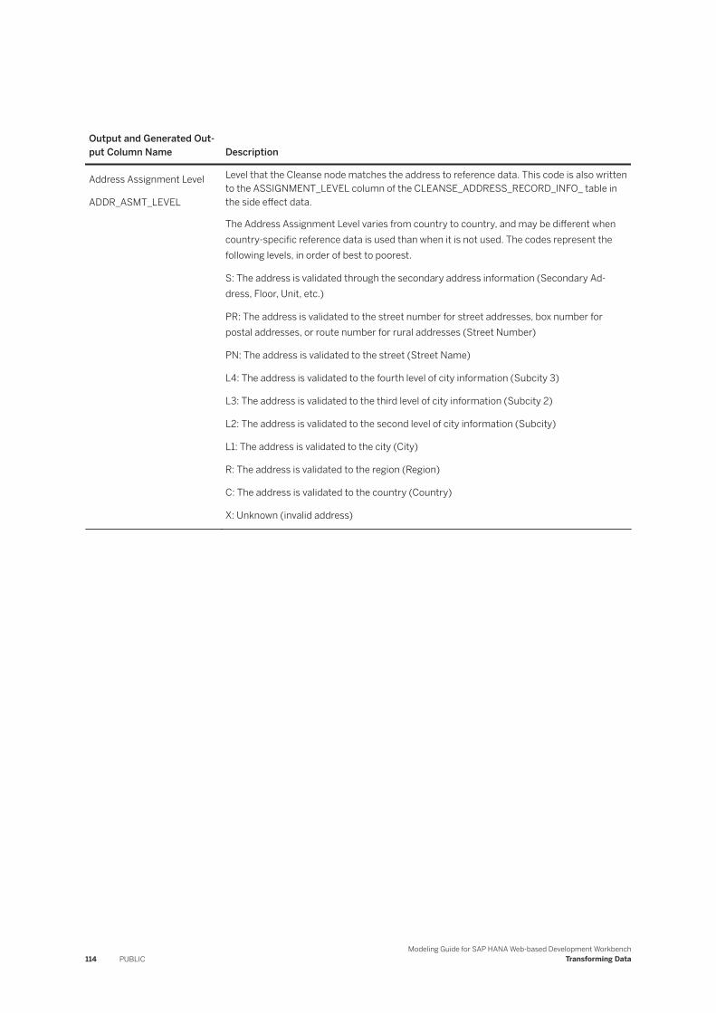
Output and Generated Output Column Name Description
Address Assignment Level
ADDR_ASMT_LEVEL
Level that the Cleanse node matches the address to reference data. This code is also written to the ASSIGNMENT_LEVEL column of the CLEANSE_ADDRESS_RECORD_INFO_ table in the side effect data.
The Address Assignment Level varies from country to country, and may be different when country-specific reference data is used than when it is not used. The codes represent the following levels, in order of best to poorest.
S: The address is validated through the secondary address information (Secondary Address, Floor, Unit, etc.)
PR: The address is validated to the street number for street addresses, box number for postal addresses, or route number for rural addresses (Street Number)
PN: The address is validated to the street (Street Name)
L4: The address is validated to the fourth level of city information (Subcity 3)
L3: The address is validated to the third level of city information (Subcity 2)
L2: The address is validated to the second level of city information (Subcity)
L1: The address is validated to the city (City)
R: The address is validated to the region (Region)
C: The address is validated to the country (Country)
X: Unknown (invalid address)
114 PUBLICModeling Guide for SAP HANA Web-based Development Workbench
Transforming Data

Output and Generated Output Column Name Description
Address Assignment Type
ADDR_ASMT_TYPE
Type of address. This code is also written to the ASSIGNMENT_TYPE column of the CLEANSE_ADDRESS_RECORD_INFO_ table in the side effect data.
BN: Building name
F: Firm
G: General delivery
H: High-rise building
HB: House boat
L: Lot
M: Military
R: Rural
P: Postal
PI: Point of reference
PS: Packstation or Paketbox
RP: Postal served by route
S: Street
SR: Street served by route
U: Uninhabited
W: Caravan
X: Unknown (invalid address)
Address Information Code
ADDR_INFO_CODE
Code that the Cleanse node generates only for addresses that are either invalid or have data that appears to be suspect. This code is also written to the INFO_CODE column of the CLEANSE_INFO_CODES_ table in the side effect data.
Modeling Guide for SAP HANA Web-based Development WorkbenchTransforming Data PUBLIC 115
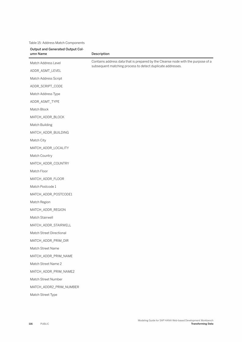
Table 15: Address Match Components
Output and Generated Output Column Name Description
Match Address Level
ADDR_ASMT_LEVEL
Match Address Script
ADDR_SCRIPT_CODE
Match Address Type
ADDR_ASMT_TYPE
Match Block
MATCH_ADDR_BLOCK
Match Building
MATCH_ADDR_BUILDING
Match City
MATCH_ADDR_LOCALITY
Match Country
MATCH_ADDR_COUNTRY
Match Floor
MATCH_ADDR_FLOOR
Match Postcode 1
MATCH_ADDR_POSTCODE1
Match Region
MATCH_ADDR_REGION
Match Stairwell
MATCH_ADDR_STAIRWELL
Match Street Directional
MATCH_ADDR_PRIM_DIR
Match Street Name
MATCH_ADDR_PRIM_NAME
Match Street Name 2
MATCH_ADDR_PRIM_NAME2
Match Street Number
MATCH_ADDR2_PRIM_NUMBER
Match Street Type
Contains address data that is prepared by the Cleanse node with the purpose of a subsequent matching process to detect duplicate addresses.
116 PUBLICModeling Guide for SAP HANA Web-based Development Workbench
Transforming Data
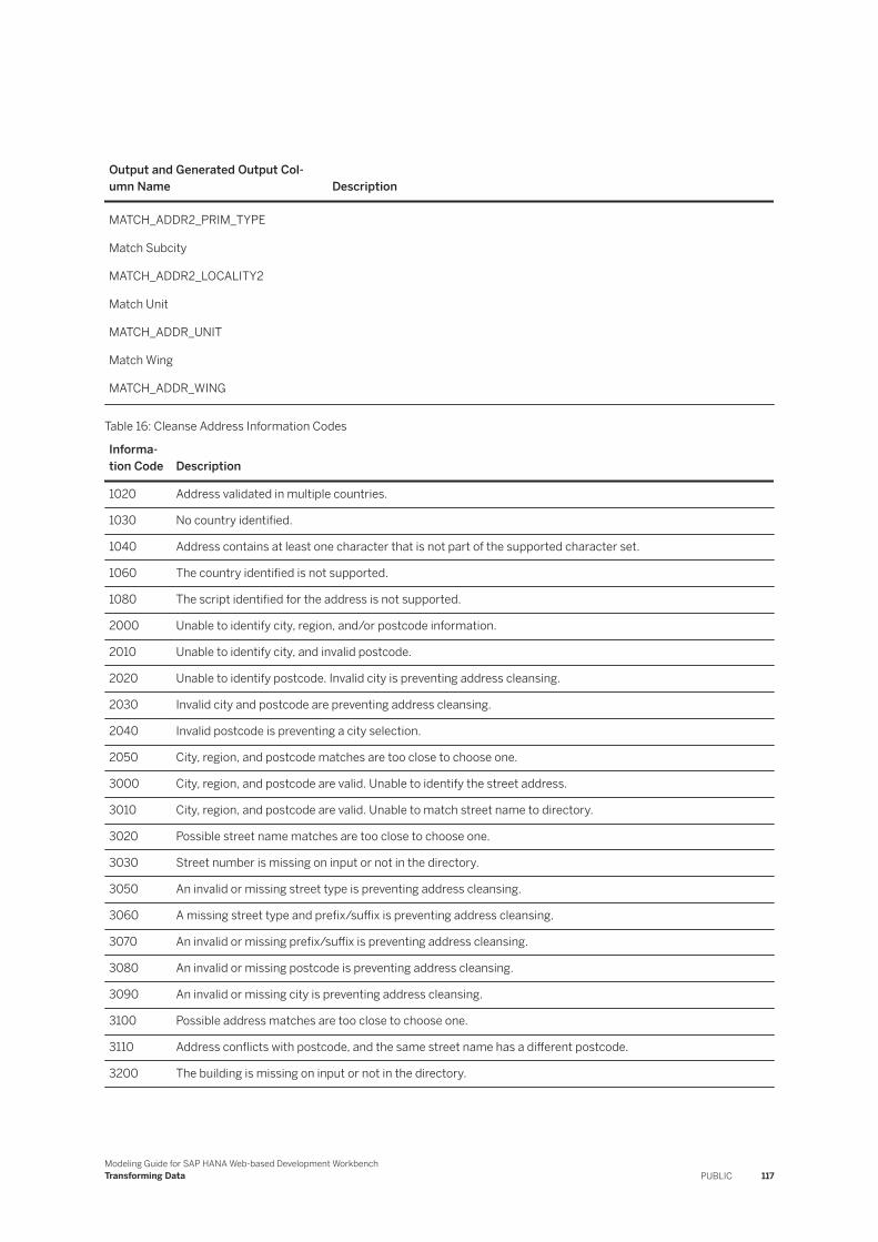
Output and Generated Output Column Name Description
MATCH_ADDR2_PRIM_TYPE
Match Subcity
MATCH_ADDR2_LOCALITY2
Match Unit
MATCH_ADDR_UNIT
Match Wing
MATCH_ADDR_WING
Table 16: Cleanse Address Information Codes
Information Code Description
1020 Address validated in multiple countries.
1030 No country identified.
1040 Address contains at least one character that is not part of the supported character set.
1060 The country identified is not supported.
1080 The script identified for the address is not supported.
2000 Unable to identify city, region, and/or postcode information.
2010 Unable to identify city, and invalid postcode.
2020 Unable to identify postcode. Invalid city is preventing address cleansing.
2030 Invalid city and postcode are preventing address cleansing.
2040 Invalid postcode is preventing a city selection.
2050 City, region, and postcode matches are too close to choose one.
3000 City, region, and postcode are valid. Unable to identify the street address.
3010 City, region, and postcode are valid. Unable to match street name to directory.
3020 Possible street name matches are too close to choose one.
3030 Street number is missing on input or not in the directory.
3050 An invalid or missing street type is preventing address cleansing.
3060 A missing street type and prefix/suffix is preventing address cleansing.
3070 An invalid or missing prefix/suffix is preventing address cleansing.
3080 An invalid or missing postcode is preventing address cleansing.
3090 An invalid or missing city is preventing address cleansing.
3100 Possible address matches are too close to choose one.
3110 Address conflicts with postcode, and the same street name has a different postcode.
3200 The building is missing on input or not in the directory.
Modeling Guide for SAP HANA Web-based Development WorkbenchTransforming Data PUBLIC 117
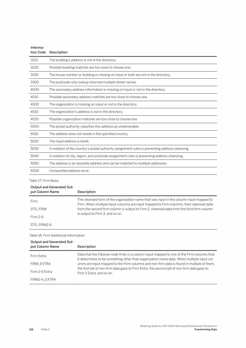
Information Code Description
3210 The building’s address is not in the directory.
3220 Possible building matches are too close to choose one.
3250 The house number or building is missing on input or both are not in the directory.
3300 The postcode-only lookup returned multiple street names.
4000 The secondary address information is missing on input or not in the directory.
4010 Possible secondary address matches are too close to choose one.
4500 The organization is missing on input or not in the directory.
4510 The organization’s address is not in the directory.
4520 Possible organization matches are too close to choose one.
5000 The postal authority classifies this address as undeliverable.
5010 The address does not reside in the specified country.
5020 The input address is blank.
5030 A violation of the country’s postal authority assignment rules is preventing address cleansing.
5040 A violation of city, region, and postcode assignment rules is preventing address cleansing.
5050 The address is an obsolete address and can be matched to multiple addresses.
6000 Unclassified address error.
Table 17: Firm Basic
Output and Generated Output Column Name Description
Firm
STD_FIRM
Firm 2-6
STD_FIRM2-6
The cleansed form of the organization name that was input in the column input mapped to Firm. When multiple input columns are input mapped to Firm columns, then cleansed data from the second firm column is output to Firm 2, cleansed data from the third firm column is output to Firm 3, and so on.
Table 18: Firm Additional Information
Output and Generated Output Column Name Description
Firm Extra
FIRM_EXTRA
Firm 2-6 Extra
FIRM2-6_EXTRA
Data that the Cleanse node finds in a column input mapped to one of the Firm columns that it determines to be something other than organization name data. When multiple input columns are input mapped to the Firm columns and non-firm data is found in multiple of them, the first set of non-firm data goes to Firm Extra, the second set of non-firm data goes to Firm 2 Extra, and so on.
118 PUBLICModeling Guide for SAP HANA Web-based Development Workbench
Transforming Data
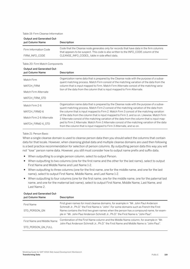
Table 19: Firm Cleanse Information
Output and Generated Output Column Name Description
Firm Information Code
FIRM_INFO_CODE
Code that the Cleanse node generates only for records that have data in the firm columns that appears to be suspect. This code is also written to the INFO_CODE column of the CLEANSE_INFO_CODES_ table in side effect data.
Table 20: Firm Match Components
Output and Generated Output Column Name Description
Match Firm
MATCH_FIRM
Match Firm Alternate
MATCH_FIRM_STD
Organization name data that is prepared by the Cleanse node with the purpose of a subsequent matching process. Match Firm consist of the matching variation of the data from the column that is input mapped to Firm. Match Firm Alternate consist of the matching variation of the data from the column that is input mapped to Firm Alternate.
Match Firm 2-6
MATCH_FIRM2-6
Match Firm 2-6 Alternate
MATCH_FIRM2-6_STD
Organization name data that is prepared by the Cleanse node with the purpose of a subsequent matching process. Match Firm 2 consist of the matching variation of the data from the column that is input mapped to Firm 2. Match Firm 3 consist of the matching variation of the data from the column that is input mapped to Firm 3, and so on. Likewise, Match Firm 2 Alternate consist of the matching variation of the data from the column that is input mapped to Firm 2 Alternate. Match Firm 3 Alternate consist of the matching variation of the data from the column that is input mapped to Firm 3 Alternate, and so on.
Table 21: Person BasicWhen a single cleanse domain is used to cleanse person data then you should select the columns that contain data for that locale. However, when cleansing global data and multiple cleanse domains are used then following is a best practice recommendation for selection of person columns. By outputting person data this way you will not “lose” person name data. However, you still must consider how to output name prefix and suffix data.
● When outputting to a single person column, select to output Person.● When outputting to two columns (one for the first name and the other for the last name), select to output
First Name and Middle Name and Last Name 1-2.● When outputting to three columns (one for the first name, one for the middle name, and one for the last
name), select to output First Name, Middle Name, and Last Name 1-2.● When outputting to four columns (one for the first name, one for the middle name, one for the paternal last
name, and one for the maternal last name), select to output First Name, Middle Name, Last Name, and Last Name 2.
Output and Generated Output Column Name Description
First Name
STD_PERSON_GN
First given names for most cleanse domains, for example in “Mr. John Paul Anderson Schmidt Jr., Ph.D.” the First Name is “John”. For some domains such as French the First Name contains the first two given names when the person has a compound name, for example in “Mr. John Paul Anderson Schmidt Jr., Ph.D.” the First Name is “John Paul”.
First Name and Middle Name
STD_PERSON_GN_FULL
Combination of the First Name column and the Middle Name column, for example in “Mr. John Paul Anderson Schmidt Jr., Ph.D.” the First Name and Middle Name is “John Paul”.
Modeling Guide for SAP HANA Web-based Development WorkbenchTransforming Data PUBLIC 119
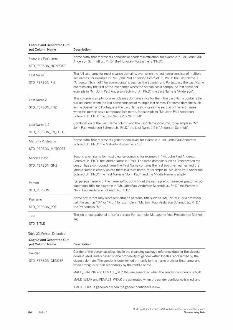
Output and Generated Output Column Name Description
Honorary Postname
STD_PERSON_HONPOST
Name suffix that represents honorific or academic affiliation, for example in “Mr. John Paul Anderson Schmidt Jr., Ph.D.” the Honorary Postname is “Ph.D.”.
Last Name
STD_PERSON_FN
The full last name for most cleanse domains, even when the last name consists of multiple last names, for example in “Mr. John Paul Anderson Schmidt Jr., Ph.D.” the Last Name is “Anderson Schmidt”. For some domains such as the Spanish and Portuguese the Last Name contains only the first of the last names when the person has a compound last name, for example in “Mr. John Paul Anderson Schmidt Jr., Ph.D.” the Last Name is “Anderson”.
Last Name 2
STD_PERSON_FN2
This column is empty for most cleanse domains since for them the Last Name contains the full last name when the last name consists of multiple last names. For some domains such as the Spanish and Portuguese the Last Name 2 contains the second of the last names when the person has a compound last name, for example in “Mr. John Paul Anderson Schmidt Jr., Ph.D.” the Last Name 2 is “Schmidt”.
Last Name 1-2
STD_PERSON_FN_FULL
Combination of the Last Name column and the Last Name 2 column, for example in “Mr. John Paul Anderson Schmidt Jr., Ph.D.” the Last Name 1-2 is “Anderson Schmidt”.
Maturity Postname
STD_PERSON_MATPOST
Name suffix that represents generational level, for example in “Mr. John Paul Anderson Schmidt Jr., Ph.D.” the Maturity Postname is “Jr.”.
Middle Name
STD_PERSON_GN2
Second given name for most cleanse domains, for example in “Mr. John Paul Anderson Schmidt Jr., Ph.D” the Middle Name is “Paul”. For some domains such as French when the person has a compound name the First Name contains the first two given names and the Middle Name is empty unless there is a third name, for example in “Mr. John Paul Anderson Schmidt Jr., Ph.D.” the First Name is “John Paul” and the Middle Name is empty.
Person
STD_PERSON
Full person name with the name suffix, but without the name prefix, name designator, or occupational title, for example in “Mr. John Paul Anderson Schmidt Jr., Ph.D.” the Person is “John Paul Anderson Schmidt Jr., Ph.D.”.
Prename
STD_PERSON_PRE
Name prefix that may represent either a personal title such as “Mr.” or “Ms.” or a professional title such as “Dr.” or “Prof.”, for example in “Mr. John Paul Anderson Schmidt Jr., Ph.D.” the Prename is “Mr.”.
Title
STD_TITLE
The job or occupational title of a person. For example, Manager or Vice President of Marketing.
Table 22: Person Extended
Output and Generated Output Column Name Description
Gender
STD_PERSON_GENDER
Gender of the person as classified in the cleansing package reference data for the cleanse domain used, and is based on the probability of gender within locales represented by the cleanse domain. The gender is determined primarily by the name prefix or first name, and when ambiguous then secondarily by the middle name.
MALE_STRONG and FEMALE_STRONG are generated when the gender confidence is high.
MALE_WEAK and FEMALE_WEAK are generated when the gender confidence is medium.
AMBIGUOUS is generated when the gender confidence is low.
120 PUBLICModeling Guide for SAP HANA Web-based Development Workbench
Transforming Data

Output and Generated Output Column Name Description
Name Designator
STD_PERSON_NDES
Designator that may be input with the person name, for example in “Attn: John Anderson” the Name Designator is “Attn:”.
Person 2
STD_PERSON2
Name of the second person when data is input with two person names, for example in “John and Mary Anderson” the Person is “John Anderson” and the Person 2 is “Mary Anderson”, and in “Gurvinder Singh s/o Sh. Tejveer Singh” the Person is “Gurvinder Singh” and the Person 2 is “Tejveer Singh”.
Title
STD_TITLE
Occupational title that may be input with the person name or instead of the person name, for example in “John Anderson, Director” the Title is “Director”.
Table 23: Person Additional Information
Output and Generated Output Column Name Description
Person Extra
PERSON_EXTRA
Data that the Cleanse node finds in a column input mapped to Person that it determines to be something other than person name data.
Table 24: Person Cleanse Information
Output and Generated Output Column Name Description
Person Information Code
PERSON_INFO_CODE
Code that the Cleanse node generates only for records that have data in the person columns that appears to be suspect. This code is also written to the INFO_CODE column of the CLEANSE_INFO_CODES_ table in the side effect data.
Modeling Guide for SAP HANA Web-based Development WorkbenchTransforming Data PUBLIC 121
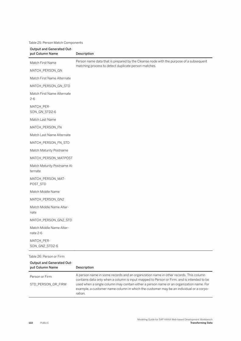
Table 25: Person Match Components
Output and Generated Output Column Name Description
Match First Name
MATCH_PERSON_GN
Match First Name Alternate
MATCH_PERSON_GN_STD
Match First Name Alternate 2-6
MATCH_PERSON_GN_STD2-6
Match Last Name
MATCH_PERSON_FN
Match Last Name Alternate
MATCH_PERSON_FN_STD
Match Maturity Postname
MATCH_PERSON_MATPOST
Match Maturity Postname Alternate
MATCH_PERSON_MATPOST_STD
Match Middle Name
MATCH_PERSON_GN2
Match Middle Name Alternate
MATCH_PERSON_GN2_STD
Match Middle Name Alternate 2-6
MATCH_PERSON_GN2_STD2-6
Person name data that is prepared by the Cleanse node with the purpose of a subsequent matching process to detect duplicate person matches.
Table 26: Person or Firm
Output and Generated Output Column Name Description
Person or Firm
STD_PERSON_OR_FIRM
A person name in some records and an organization name in other records. This column contains data only when a column is input mapped to Person or Firm, and is intended to be used when a single column may contain either a person name or an organization name. For example, a customer name column in which the customer may be an individual or a corporation.
122 PUBLICModeling Guide for SAP HANA Web-based Development Workbench
Transforming Data

Output and Generated Output Column Name Description
Person or Firm Extra
PERSON_OR_FIRM_EXTRA
Includes extraneous information such as Inc., Esq., and so on.
Table 27: Person or Firm Match Components
Output and Generated Output Column Name Description
Match Person
MATCH_PERSON
Person or firm name data that is prepared by the Cleanse node with the purpose of a subsequent matching process to detect duplicate person matches.
Table 28: Cleanse Person or Firm Information Codes
Information Code Description
P101 The person name contains data not in the dictionary.
P102 The person name contains data similar to organization name data.
P103 The person name is not typical of person name data.
P104 The first name is missing, initialized, or questionable.
P105 The last name is missing, initialized, or questionable.
P151 The job title contains data not in the dictionary.
P201 The person name contains data not in the dictionary.
P202 The person name contains data similar to organization name data.
P203 The person name is not typical of person name data.
P204 The first name is missing, initialized, or questionable.
P205 The last name is missing, initialized, or questionable.
P251 The job title contains data not in the dictionary.
F101 The organization name contains data not in the dictionary.
F102 The organization name contains data similar to person name data.
F103 The organization name is not typical of organization name data.
F201 The organization name contains data not in the dictionary.
F202 The organization name contains data similar to person name data.
F203 The organization name is not typical of firm name data.
F301 The organization name contains data not in the dictionary.
F302 The organization name contains data similar to person name data.
F303 The organization name is not typical of organization name data.
F401 The organization name contains data not in the dictionary.
F402 The organization name contains data similar to person name data.
Modeling Guide for SAP HANA Web-based Development WorkbenchTransforming Data PUBLIC 123
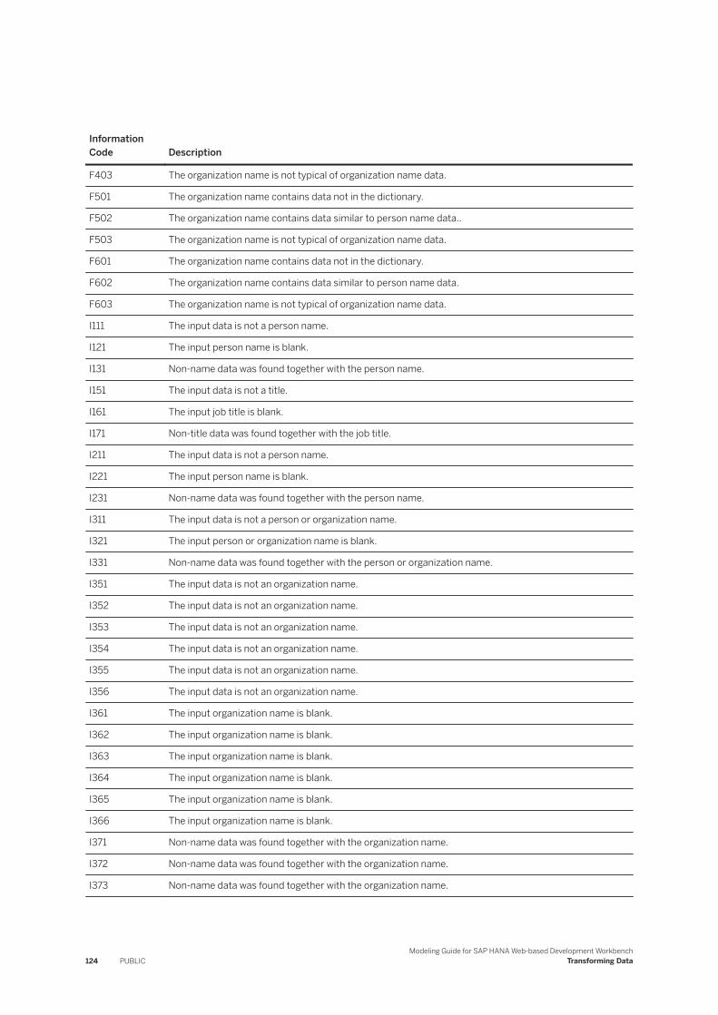
Information Code Description
F403 The organization name is not typical of organization name data.
F501 The organization name contains data not in the dictionary.
F502 The organization name contains data similar to person name data..
F503 The organization name is not typical of organization name data.
F601 The organization name contains data not in the dictionary.
F602 The organization name contains data similar to person name data.
F603 The organization name is not typical of organization name data.
I111 The input data is not a person name.
I121 The input person name is blank.
I131 Non-name data was found together with the person name.
I151 The input data is not a title.
I161 The input job title is blank.
I171 Non-title data was found together with the job title.
I211 The input data is not a person name.
I221 The input person name is blank.
I231 Non-name data was found together with the person name.
I311 The input data is not a person or organization name.
I321 The input person or organization name is blank.
I331 Non-name data was found together with the person or organization name.
I351 The input data is not an organization name.
I352 The input data is not an organization name.
I353 The input data is not an organization name.
I354 The input data is not an organization name.
I355 The input data is not an organization name.
I356 The input data is not an organization name.
I361 The input organization name is blank.
I362 The input organization name is blank.
I363 The input organization name is blank.
I364 The input organization name is blank.
I365 The input organization name is blank.
I366 The input organization name is blank.
I371 Non-name data was found together with the organization name.
I372 Non-name data was found together with the organization name.
I373 Non-name data was found together with the organization name.
124 PUBLICModeling Guide for SAP HANA Web-based Development Workbench
Transforming Data

Information Code Description
I374 Non-name data was found together with the organization name.
I375 Non-name data was found together with the organization name.
I376 Non-name data was found together with the organization name.
Table 29: Phone
Output and Generated Output Column Name Description
Phone
STD_PHONE
Phone 2-6
STD_PHONE2-6
The cleansed form of the phone number found mapped to the corresponding Phone output column.
Table 30: Phone Additional
Output and Generated Output Column Name Description
Phone Extra
PHONE_EXTRA
Phone 2-6 Extra
PHONE2-6_EXTRA
Data the Cleanse node finds in a column input mapped to one of the phone columns that is determined to be something other than phone number data. When multiple input columns are mapped to the Phone columns, and non-phone data is found in multiple columns, the first set of non-phone data goes to Phone Extra, the second set of non-phone data goes to Phone 2 Extra, and so on.
Table 31: Phone Cleanse Information
Output and Generated Output Column Name Description
Phone Information Code
PHONE_INFO_CODE
The code that the Cleanse node generates only for records that have data in the phone columns that appear to be suspect. This code is written in the INFO_CODE column of the CLEANSE_INFO_CODES table in side effect data. It identifies the rows that may require manual review because the data is suspect.
Table 32: Phone Match Components
Output and Generated Output Column Name Description
Match Phone
MATCH_PHONE
Match Phone 2-6
MATCH_PHONE2-6
Phone number data that is prepared by the Cleanse node with the purpose of being input to the Match node in order to detect duplicate phone numbers. Match Phone consists of the matching variation of the data from the column that is input mapped to Phone. Match Phone 2 consists of the matching variation of the data from the column that is input mapped to Phone 2, and so on.
Modeling Guide for SAP HANA Web-based Development WorkbenchTransforming Data PUBLIC 125
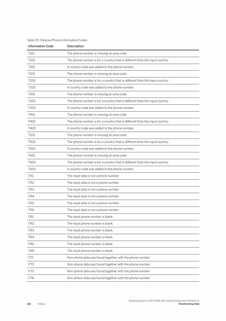
Table 33: Cleanse Phone Information Codes
Information Code Description
T101 The phone number is missing an area code.
T102 The phone number is for a country that is different than the input country.
T103 A country code was added to the phone number.
T201 The phone number is missing an area code.
T202 The phone number is for a country that is different than the input country.
T203 A country code was added to the phone number.
T301 The phone number is missing an area code.
T302 The phone number is for a country that is different than the input country.
T303 A country code was added to the phone number.
T401 The phone number is missing an area code.
T402 The phone number is for a country that is different than the input country.
T403 A country code was added to the phone number.
T501 The phone number is missing an area code.
T502 The phone number is for a country that is different than the input country.
T503 A country code was added to the phone number.
T601 The phone number is missing an area code.
T602 The phone number is for a country that is different than the input country.
T603 A country code was added to the phone number.
I751 The input data is not a phone number.
I752 The input data is not a phone number.
I753 The input data is not a phone number.
I754 The input data is not a phone number.
I755 The input data is not a phone number.
I756 The input data is not a phone number.
I761 The input phone number is blank.
I762 The input phone number is blank.
I763 The input phone number is blank.
I764 The input phone number is blank.
I765 The input phone number is blank.
I766 The input phone number is blank.
I771 Non-phone data was found together with the phone number.
I772 Non-phone data was found together with the phone number.
I773 Non-phone data was found together with the phone number.
I774 Non-phone data was found together with the phone number.
126 PUBLICModeling Guide for SAP HANA Web-based Development Workbench
Transforming Data
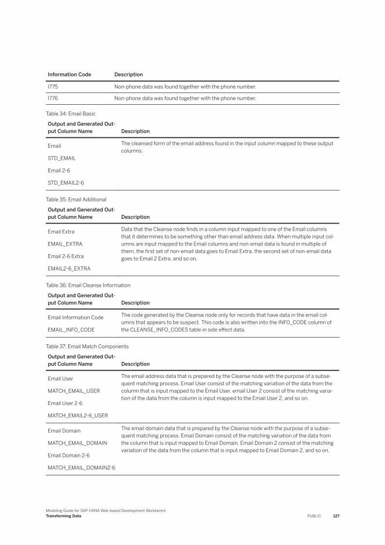
Information Code Description
I775 Non-phone data was found together with the phone number.
I776 Non-phone data was found together with the phone number.
Table 34: Email Basic
Output and Generated Output Column Name Description
STD_EMAIL
Email 2-6
STD_EMAIL2-6
The cleansed form of the email address found in the input column mapped to these output columns.
Table 35: Email Additional
Output and Generated Output Column Name Description
Email Extra
EMAIL_EXTRA
Email 2-6 Extra
EMAIL2-6_EXTRA
Data that the Cleanse node finds in a column input mapped to one of the Email columns that it determines to be something other than email address data. When multiple input columns are input mapped to the Email columns and non-email data is found in multiple of them, the first set of non-email data goes to Email Extra, the second set of non-email data goes to Email 2 Extra, and so on.
Table 36: Email Cleanse Information
Output and Generated Output Column Name Description
Email Information Code
EMAIL_INFO_CODE
The code generated by the Cleanse node only for records that have data in the email columns that appears to be suspect. This code is also written into the INFO_CODE column of the CLEANSE_INFO_CODES table in side effect data.
Table 37: Email Match Components
Output and Generated Output Column Name Description
Email User
MATCH_EMAIL_USER
Email User 2-6
MATCH_EMAIL2-6_USER
The email address data that is prepared by the Cleanse node with the purpose of a subsequent matching process. Email User consist of the matching variation of the data from the column that is input mapped to the Email User. email User 2 consist of the matching variation of the data from the column is input mapped to the Email User 2, and so on.
Email Domain
MATCH_EMAIL_DOMAIN
Email Domain 2-6
MATCH_EMAIL_DOMAIN2-6
The email domain data that is prepared by the Cleanse node with the purpose of a subsequent matching process. Email Domain consist of the matching variation of the data from the column that is input mapped to Email Domain. Email Domain 2 consist of the matching variation of the data from the column that is input mapped to Email Domain 2, and so on.
Modeling Guide for SAP HANA Web-based Development WorkbenchTransforming Data PUBLIC 127
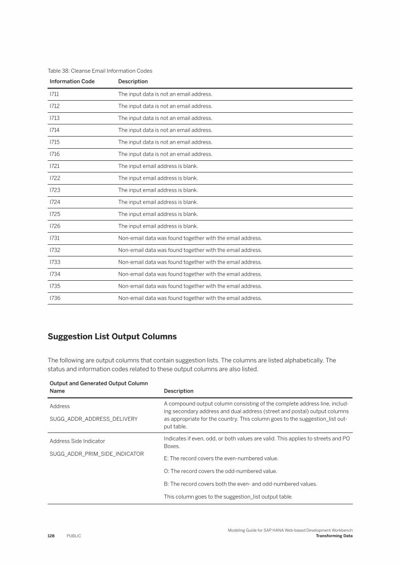
Table 38: Cleanse Email Information Codes
Information Code Description
I711 The input data is not an email address.
I712 The input data is not an email address.
I713 The input data is not an email address.
I714 The input data is not an email address.
I715 The input data is not an email address.
I716 The input data is not an email address.
I721 The input email address is blank.
I722 The input email address is blank.
I723 The input email address is blank.
I724 The input email address is blank.
I725 The input email address is blank.
I726 The input email address is blank.
I731 Non-email data was found together with the email address.
I732 Non-email data was found together with the email address.
I733 Non-email data was found together with the email address.
I734 Non-email data was found together with the email address.
I735 Non-email data was found together with the email address.
I736 Non-email data was found together with the email address.
Suggestion List Output Columns
The following are output columns that contain suggestion lists. The columns are listed alphabetically. The status and information codes related to these output columns are also listed.
Output and Generated Output Column Name Description
Address
SUGG_ADDR_ADDRESS_DELIVERY
A compound output column consisting of the complete address line, including secondary address and dual address (street and postal) output columns as appropriate for the country. This column goes to the suggestion_list output table.
Address Side Indicator
SUGG_ADDR_PRIM_SIDE_INDICATOR
Indicates if even, odd, or both values are valid. This applies to streets and PO Boxes.
E: The record covers the even-numbered value.
O: The record covers the odd-numbered value.
B: The record covers both the even- and odd-numbered values.
This column goes to the suggestion_list output table.
128 PUBLICModeling Guide for SAP HANA Web-based Development Workbench
Transforming Data
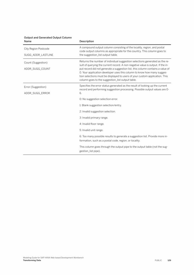
Output and Generated Output Column Name Description
City Region Postcode
SUGG_ADDR_LASTLINE
A compound output column consisting of the locality, region, and postal code output columns as appropriate for the country. This column goes to the suggestion_list output table.
Count (Suggestion)
ADDR_SUGG_COUNT
Returns the number of individual suggestion selections generated as the result of querying the current record. A non-negative value is output. If the input record did not generate a suggestion list, this column contains a value of 0. Your application developer uses this column to know how many suggestion selections must be displayed to users of your custom application. This column goes to the suggestion_list output table.
Error (Suggestion)
ADDR_SUGG_ERROR
Specifies the error status generated as the result of looking up the current record and performing suggestion processing. Possible output values are 0- 6.
0: No suggestion selection error.
1: Blank suggestion selection/entry.
2: Invalid suggestion selection.
3: Invalid primary range.
4: Invalid floor range.
5: Invalid unit range.
6: Too many possible results to generate a suggestion list. Provide more information, such as a postal code, region, or locality.
This column goes through the output pipe to the output table (not the suggestion_list pipe).
Modeling Guide for SAP HANA Web-based Development WorkbenchTransforming Data PUBLIC 129
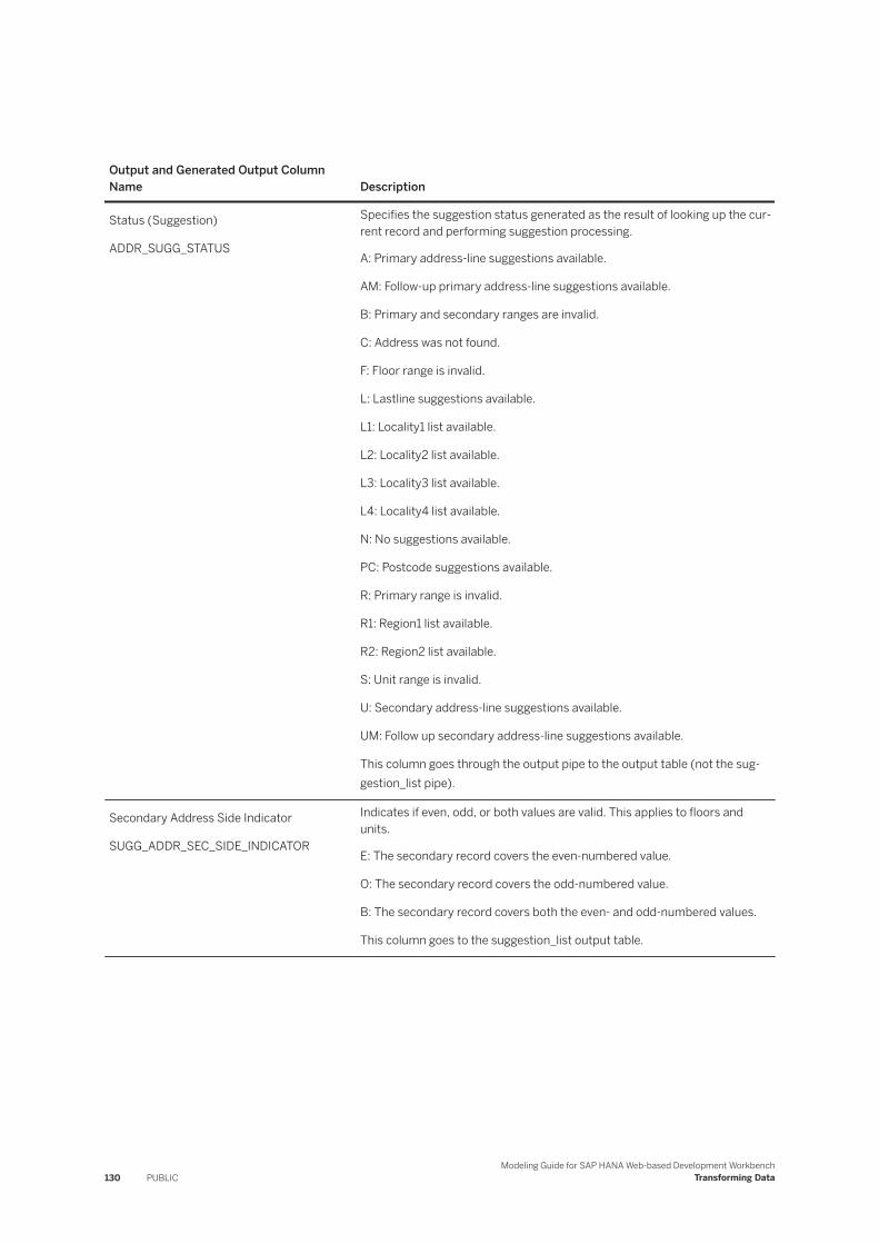
Output and Generated Output Column Name Description
Status (Suggestion)
ADDR_SUGG_STATUS
Specifies the suggestion status generated as the result of looking up the current record and performing suggestion processing.
A: Primary address-line suggestions available.
AM: Follow-up primary address-line suggestions available.
B: Primary and secondary ranges are invalid.
C: Address was not found.
F: Floor range is invalid.
L: Lastline suggestions available.
L1: Locality1 list available.
L2: Locality2 list available.
L3: Locality3 list available.
L4: Locality4 list available.
N: No suggestions available.
PC: Postcode suggestions available.
R: Primary range is invalid.
R1: Region1 list available.
R2: Region2 list available.
S: Unit range is invalid.
U: Secondary address-line suggestions available.
UM: Follow up secondary address-line suggestions available.
This column goes through the output pipe to the output table (not the suggestion_list pipe).
Secondary Address Side Indicator
SUGG_ADDR_SEC_SIDE_INDICATOR
Indicates if even, odd, or both values are valid. This applies to floors and units.
E: The secondary record covers the even-numbered value.
O: The secondary record covers the odd-numbered value.
B: The secondary record covers both the even- and odd-numbered values.
This column goes to the suggestion_list output table.
130 PUBLICModeling Guide for SAP HANA Web-based Development Workbench
Transforming Data
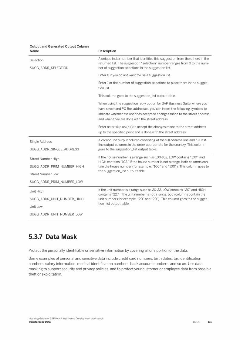
Output and Generated Output Column Name Description
Selection
SUGG_ADDR_SELECTION
A unique index number that identifies this suggestion from the others in the returned list. The suggestion “selection” number ranges from 0 to the number of suggestion selections in the suggestion list.
Enter 0 if you do not want to use a suggestion list.
Enter 1 or the number of suggestion selections to place them in the suggestion list.
This column goes to the suggestion_list output table.
When using the suggestion reply option for SAP Business Suite, where you have street and PO Box addresses, you can insert the following symbols to indicate whether the user has accepted changes made to the street address, and when they are done with the street address.
Enter asterisk plus (*+) to accept the changes made to the street address up to the specified point and is done with the street address.
Single Address
SUGG_ADDR_SINGLE_ADDRESS
A compound output column consisting of the full address-line and full last-line output columns in the order appropriate for the country. This column goes to the suggestion_list output table.
Street Number High
SUGG_ADDR_PRIM_NUMBER_HIGH
Street Number Low
SUGG_ADDR_PRIM_NUMBER_LOW
If the house number is a range such as 100-102, LOW contains “100” and HIGH contains “102.” If the house number is not a range, both columns contain the house number (for example, “100” and “100”). This column goes to the suggestion_list output table.
Unit High
SUGG_ADDR_UNIT_NUMBER_HIGH
Unit Low
SUGG_ADDR_UNIT_NUMBER_LOW
If the unit number is a range such as 20-22, LOW contains “20” and HIGH contains “22.” If the unit number is not a range, both columns contain the unit number (for example, “20” and “20”). This column goes to the suggestion_list output table.
5.3.7 Data Mask
Protect the personally identifiable or sensitive information by covering all or a portion of the data.
Some examples of personal and sensitive data include credit card numbers, birth dates, tax identification numbers, salary information, medical identification numbers, bank account numbers, and so on. Use data masking to support security and privacy policies, and to protect your customer or employee data from possible theft or exploitation.
Modeling Guide for SAP HANA Web-based Development WorkbenchTransforming Data PUBLIC 131
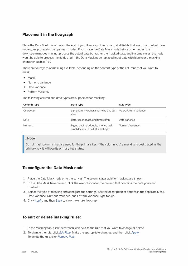
Placement in the flowgraph
Place the Data Mask node toward the end of your flowgraph to ensure that all fields that are to be masked have undergone processing by upstream nodes. If you place the Data Mask node before other nodes, the downstream nodes may not process the actual data but rather the masked data, and in some cases, the node won’t be able to process the fields at all if the Data Mask node replaced input data with blanks or a masking character such as “#”.
There are four types of masking available, depending on the content type of the columns that you want to mask.
● Mask● Numeric Variance● Date Variance● Pattern Variance
The following column and data types are supported for masking.
Column Type Data Type Rule Type
Character alphanum, nvarchar, shorttext, and varchar
Mask, Pattern Variance
Date date, seconddate, and timestamp Date Variance
Numeric bigint, decimal, double, integer, real, smalldecimal, smallint, and tinyint
Numeric Variance
NoteDo not mask columns that are used for the primary key. If the column you're masking is designated as the primary key, it will lose its primary key status.
To configure the Data Mask node:
1. Place the Data Mask node onto the canvas. The columns available for masking are shown.2. In the Data Mask Rule column, click the wrench icon for the column that contains the data you want
masked.3. Select the type of masking and configure the settings. See the description of options in the separate Mask,
Date Variance, Numeric Variance, and Pattern Variance Type topics.4. Click Apply, and then Back to view the entire flowgraph.
To edit or delete masking rules:
1. In the Masking tab, click the wrench icon next to the rule that you want to change or delete.2. To change the rule, click Edit Rule. Make the appropriate changes, and then click Apply.
To delete the rule, click Remove Rule.
132 PUBLICModeling Guide for SAP HANA Web-based Development Workbench
Transforming Data

Related Information
Change Default Data Mask Settings [page 133]Mask Type [page 137]Date Variance Type [page 138]Numeric Variance Type [page 141]Pattern Variance Type [page 143]
5.3.7.1 Change Default Data Mask Settings
Set the default format and language when the data is ambiguous, and set the seed value to ensure referential integrity.
Context
When the input date data is vague or ambiguous, the Data Mask node outputs the format and language you specify here. For example, if your Last_Updated column has the date "2016-04-12", depending on the date format for the country, the date could be April 12, 2016, or it could be December 4, 2016. Setting the default Date format to Year Day Month ensures that the output data refers to December 4, 2016.
When you want to maintain referential integrity, set the Seed option. This still masks the data, but in a way that ensures consistent values each time the data is output. Let's say that you mask the Customer_ID value and you want to ensure each ID is randomized on output. You can use any combination of numbers and characters to create an identifiable value such as Region9_Cust. This value is not output; it simply ensures that the output data is consistent each time the flowgraph runs. For example, you might run a Numeric Variance with a Fixed Number and have set the Variance option to 5.
Input data Valid output range
2550 2545-2555
3000 2995-3005
5500 4595-5505
After the first run, let's say the output data is:
Output data after initial processing
2552
3001
5505
With the seed value set, the subsequent processing keeps the same output for each record. Without setting the seed value, the output continues to be randomized.
Modeling Guide for SAP HANA Web-based Development WorkbenchTransforming Data PUBLIC 133
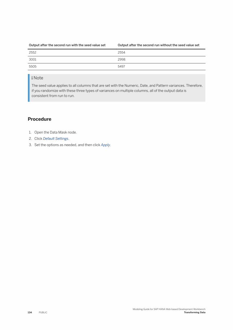
Output after the second run with the seed value set Output after the second run without the seed value set
2552 2554
3001 2998
5505 5497
NoteThe seed value applies to all columns that are set with the Numeric, Date, and Pattern variances. Therefore, if you randomize with these three types of variances on multiple columns, all of the output data is consistent from run to run.
Procedure
1. Open the Data Mask node.2. Click Default Settings.3. Set the options as needed, and then click Apply.
134 PUBLICModeling Guide for SAP HANA Web-based Development Workbench
Transforming Data
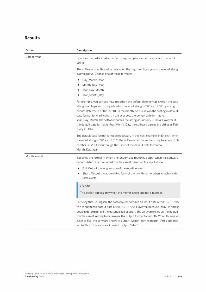
Results
Option Description
Date format Specifies the order in which month, day, and year elements appear in the input string.
The software uses this value only when the day, month, or year in the input string is ambiguous. Choose one of these formats:
● Day_Month_Year● Month_Day_Year● Year_Day_Month● Year_Month_Day
For example, you can see how important the default date format is when the date string is ambiguous. In English, when an input string is 2014/02/01, parsing cannot determine if “02” or “01” is the month, so it relies on the setting in default date format for clarification. If the user sets the default date format to Year_Day_Month, the software parses the string as January 2, 2014. However, if the default date format is Year_Month_Day, the software parses the string as February 1, 2014.
The default date format is not be necessary in this next example. In English, when the input string is 2014/31/12, the software can parse the string to a date of December 31, 2014 even though the user set the default date format to Month_Day_Year.
Month format Specifies the format in which the randomized month is output when the software cannot determine the output month format based on the input alone:
● Full: Output the long version of the month name.● Short: Output the abbreviated form of the month name, when an abbreviated
form exists.
NoteThis option applies only when the month is text and not a number.
Let's say that, in English, the software randomizes an input date of 2015/05/05 to a randomized output date of 2015/03/22. However, because “May” is ambiguous in determining if the output is full or short, the software relies on the default month format setting to determine the output format for month. When this option is set to Full, the software knows to output “March” for the month. If this option is set to Short, the software knows to output “Mar”.
Modeling Guide for SAP HANA Web-based Development WorkbenchTransforming Data PUBLIC 135
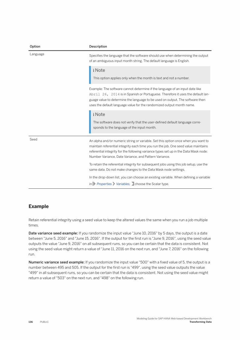
Option Description
Language Specifies the language that the software should use when determining the output of an ambiguous input month string. The default language is English.
NoteThis option applies only when the month is text and not a number.
Example: The software cannot determine if the language of an input date like Abril 26, 2014 is in Spanish or Portuguese. Therefore it uses the default language value to determine the language to be used on output. The software then uses the default language value for the randomized output month name.
NoteThe software does not verify that the user-defined default language corresponds to the language of the input month.
Seed An alpha and/or numeric string or variable. Set this option once when you want to maintain referential integrity each time you run the job. One seed value maintains referential integrity for the following variance types set up in the Data Mask node: Number Variance, Date Variance, and Pattern Variance.
To retain the referential integrity for subsequent jobs using this job setup, use the same data. Do not make changes to the Data Mask node settings.
In the drop-down list, you can choose an existing variable. When defining a variable
in Properties Variables, choose the Scalar type.
Example
Retain referential integrity using a seed value to keep the altered values the same when you run a job multiple times.
Date variance seed example: If you randomize the input value "June 10, 2016" by 5 days, the output is a date between "June 5, 2016" and "June 15, 2016". If the output for the first run is "June 9, 2016", using the seed value outputs the value "June 9, 2016" on all subsequent runs, so you can be certain that the data is consistent. Not using the seed value might return a value of "June 11, 2016 on the next run, and "June 7, 2016" on the following run.
Numeric variance seed example: If you randomize the input value "500" with a fixed value of 5, the output is a number between 495 and 505. If the output for the first run is "499", using the seed value outputs the value "499" in all subsequent runs, so you can be certain that the data is consistent. Not using the seed value might return a value of "503" on the next run, and "498" on the following run.
136 PUBLICModeling Guide for SAP HANA Web-based Development Workbench
Transforming Data
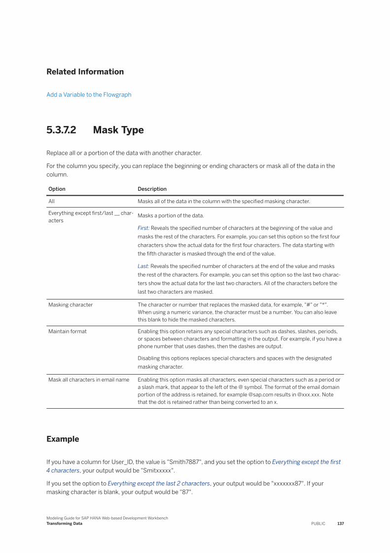
Related Information
Add a Variable to the Flowgraph
5.3.7.2 Mask Type
Replace all or a portion of the data with another character.
For the column you specify, you can replace the beginning or ending characters or mask all of the data in the column.
Option Description
All Masks all of the data in the column with the specified masking character.
Everything except first/last __ characters
Masks a portion of the data.
First: Reveals the specified number of characters at the beginning of the value and masks the rest of the characters. For example, you can set this option so the first four characters show the actual data for the first four characters. The data starting with the fifth character is masked through the end of the value.
Last: Reveals the specified number of characters at the end of the value and masks the rest of the characters. For example, you can set this option so the last two characters show the actual data for the last two characters. All of the characters before the last two characters are masked.
Masking character The character or number that replaces the masked data, for example, "#" or "*". When using a numeric variance, the character must be a number. You can also leave this blank to hide the masked characters.
Maintain format Enabling this option retains any special characters such as dashes, slashes, periods, or spaces between characters and formatting in the output. For example, if you have a phone number that uses dashes, then the dashes are output.
Disabling this options replaces special characters and spaces with the designated masking character.
Mask all characters in email name Enabling this option masks all characters, even special characters such as a period or a slash mark, that appear to the left of the @ symbol. The format of the email domain portion of the address is retained, for example @sap.com results in @xxx.xxx. Note that the dot is retained rather than being converted to an x.
Example
If you have a column for User_ID, the value is "Smith7887", and you set the option to Everything except the first 4 characters, your output would be "Smitxxxxx".
If you set the option to Everything except the last 2 characters, your output would be "xxxxxxx87". If your masking character is blank, your output would be "87".
Modeling Guide for SAP HANA Web-based Development WorkbenchTransforming Data PUBLIC 137

Example
If you have a column for Phone1, the value is "800-555-1234", and you select Maintain format, your output would be "xxx-xxx-xxxx". Not selecting this option would output "xxxxxxxxxxxx".
Example
If you have a column for Email1, the value is "[email protected]", and you enable Maintain format and Mask all characters in email name, your output would be "[email protected]".
If you enable Maintain format and disable Mask all characters in email name, your output would be "[email protected]".
If you disable both Maintain format and Mask all characters in email name, your output would be "xxxxxxxxxxxxxxxxxx".
5.3.7.3 Date Variance Type
Use Date Variance to output randomized dates.
Set the options to alter input dates based on a date variance type, such as the number of days, months, years, or within a set range.
When using the fixed days, months, and years options, the application generates an internal calculation based on the variance number. For example, if you have an input value of "May 27, 2005" and select Fixed Months and a variance of three, then the calculated minimum and maximum dates are Feb 27, 2005 and Aug 27, 2005. If you have set a user-defined minimum date of Apr 1, 2005 (within the calculated minimum value), and a user-defined maximum date of Dec 31, 2005 (outside the calculated maximum value), then the new valid range is April 1, 2005 (the user-defined minimum) through Aug 27, 2005 (the internally calculated maximum value).
138 PUBLICModeling Guide for SAP HANA Web-based Development Workbench
Transforming Data
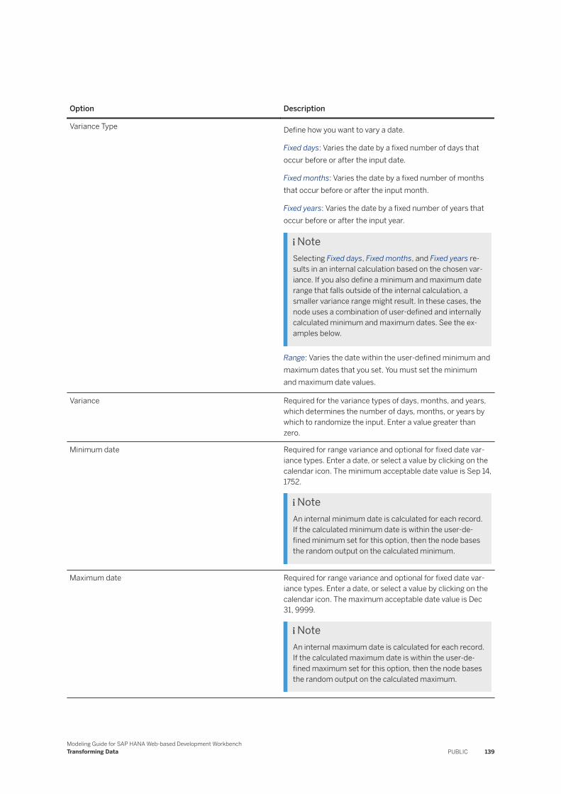
Option Description
Variance Type Define how you want to vary a date.
Fixed days: Varies the date by a fixed number of days that occur before or after the input date.
Fixed months: Varies the date by a fixed number of months that occur before or after the input month.
Fixed years: Varies the date by a fixed number of years that occur before or after the input year.
NoteSelecting Fixed days, Fixed months, and Fixed years results in an internal calculation based on the chosen variance. If you also define a minimum and maximum date range that falls outside of the internal calculation, a smaller variance range might result. In these cases, the node uses a combination of user-defined and internally calculated minimum and maximum dates. See the examples below.
Range: Varies the date within the user-defined minimum and maximum dates that you set. You must set the minimum and maximum date values.
Variance Required for the variance types of days, months, and years, which determines the number of days, months, or years by which to randomize the input. Enter a value greater than zero.
Minimum date Required for range variance and optional for fixed date variance types. Enter a date, or select a value by clicking on the calendar icon. The minimum acceptable date value is Sep 14, 1752.
NoteAn internal minimum date is calculated for each record. If the calculated minimum date is within the user-defined minimum set for this option, then the node bases the random output on the calculated minimum.
Maximum date Required for range variance and optional for fixed date variance types. Enter a date, or select a value by clicking on the calendar icon. The maximum acceptable date value is Dec 31, 9999.
NoteAn internal maximum date is calculated for each record. If the calculated maximum date is within the user-defined maximum set for this option, then the node bases the random output on the calculated maximum.
Modeling Guide for SAP HANA Web-based Development WorkbenchTransforming Data PUBLIC 139
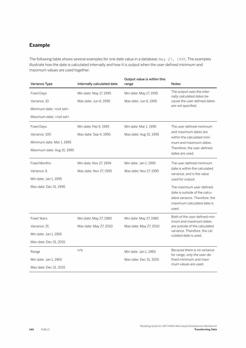
Example
The following table shows several examples for one date value in a database: May 27, 1995. The examples illustrate how the date is calculated internally and how it is output when the user-defined minimum and maximum values are used together.
Variance Type Internally calculated dateOutput value is within this range Notes
Fixed Days
Variance: 10
Minimum date: <not set>
Maximum date: <not set>
Min date: May 17, 1995
Max date: Jun 6, 1995
Min date: May 17, 1995
Max date: Jun 6, 1995
The output uses the internally calculated dates because the user-defined dates are not specified.
Fixed Days
Variance: 100
Minimum date: Mar 1, 1995
Maximum date: Aug 31, 1995
Min date: Feb 9, 1995
Max date: Sep 4, 1995
Min date: Mar 1, 1995
Max date: Aug 31, 1995
The user-defined minimum and maximum dates are within the calculated minimum and maximum dates. Therefore, the user-defined dates are used.
Fixed Months
Variance: 6
Min date: Jan 1, 1995
Max date: Dec 31, 1995
Min date: Nov 27, 1994
Max date: Nov 27, 1995
Min date: Jan 1, 1995
Max date: Nov 27, 1995
The user-defined minimum date is within the calculated variance, and is the value used for output.
The maximum user-defined date is outside of the calculated variance. Therefore, the maximum calculated date is used.
Fixed Years
Variance: 15
Min date: Jan 1, 1965
Max date: Dec 31, 2015
Min date: May 27, 1980
Max date: May 27, 2010
Min date: May 27, 1980
Max date: May 27, 2010
Both of the user-defined minimum and maximum dates are outside of the calculated variance. Therefore, the calculated date is used.
Range
Min date: Jan 1, 1965
Max date: Dec 31, 2015
n/a Min date: Jan 1, 1965
Max date: Dec 31, 2015
Because there is no variance for range, only the user-defined minimum and maximum values are used.
140 PUBLICModeling Guide for SAP HANA Web-based Development Workbench
Transforming Data
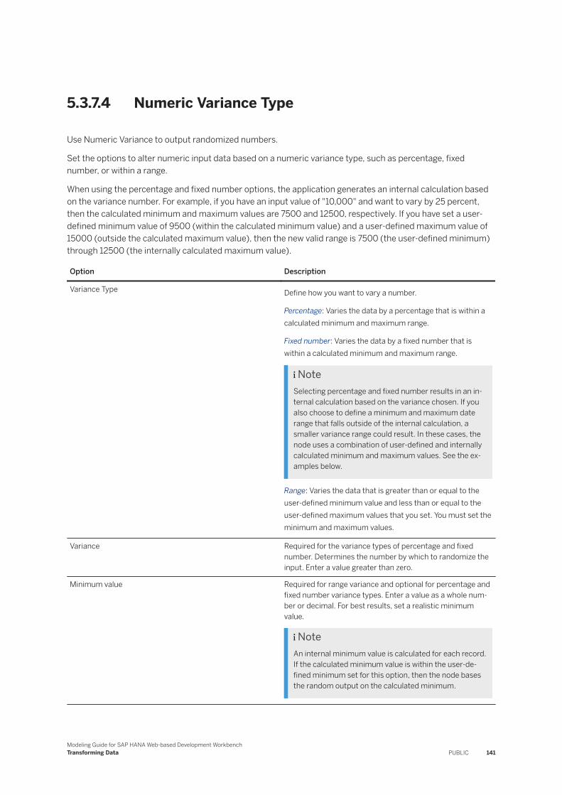
5.3.7.4 Numeric Variance Type
Use Numeric Variance to output randomized numbers.
Set the options to alter numeric input data based on a numeric variance type, such as percentage, fixed number, or within a range.
When using the percentage and fixed number options, the application generates an internal calculation based on the variance number. For example, if you have an input value of "10,000" and want to vary by 25 percent, then the calculated minimum and maximum values are 7500 and 12500, respectively. If you have set a user-defined minimum value of 9500 (within the calculated minimum value) and a user-defined maximum value of 15000 (outside the calculated maximum value), then the new valid range is 7500 (the user-defined minimum) through 12500 (the internally calculated maximum value).
Option Description
Variance Type Define how you want to vary a number.
Percentage: Varies the data by a percentage that is within a calculated minimum and maximum range.
Fixed number: Varies the data by a fixed number that is within a calculated minimum and maximum range.
NoteSelecting percentage and fixed number results in an internal calculation based on the variance chosen. If you also choose to define a minimum and maximum date range that falls outside of the internal calculation, a smaller variance range could result. In these cases, the node uses a combination of user-defined and internally calculated minimum and maximum values. See the examples below.
Range: Varies the data that is greater than or equal to the user-defined minimum value and less than or equal to the user-defined maximum values that you set. You must set the minimum and maximum values.
Variance Required for the variance types of percentage and fixed number. Determines the number by which to randomize the input. Enter a value greater than zero.
Minimum value Required for range variance and optional for percentage and fixed number variance types. Enter a value as a whole number or decimal. For best results, set a realistic minimum value.
NoteAn internal minimum value is calculated for each record. If the calculated minimum value is within the user-defined minimum set for this option, then the node bases the random output on the calculated minimum.
Modeling Guide for SAP HANA Web-based Development WorkbenchTransforming Data PUBLIC 141
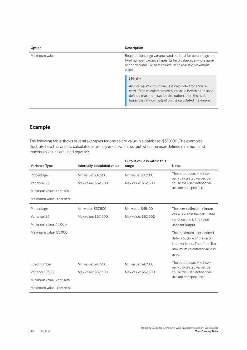
Option Description
Maximum value Required for range variance and optional for percentage and fixed number variance types. Enter a value as a whole number or decimal. For best results, set a realistic maximum value.
NoteAn internal maximum value is calculated for each record. If the calculated maximum value is within the user-defined maximum set for this option, then the node bases the random output on the calculated maximum.
Example
The following table shows several examples for one salary value in a database: $50,000. The examples illustrate how the value is calculated internally and how it is output when the user-defined minimum and maximum values are used together.
Variance Type Internally calculated valueOutput value is within this range Notes
Percentage
Variance: 25
Minimum value: <not set>
Maximum value: <not set>
Min value: $37,500
Max value: $62,500
Min value: $37,500
Max value: $62,500
The output uses the internally calculated values because the user-defined values are not specified.
Percentage
Variance: 25
Minimum value: 45,000
Maximum value: 85,000
Min value: $37,500
Max value: $62,500
Min value: $45, 00
Max value: $62,500
The user-defined minimum value is within the calculated variance and is the value used for output.
The maximum user-defined date is outside of the calculated variance. Therefore, the maximum calculated value is used.
Fixed number
Variance: 2500
Minimum value: <not set>
Maximum value: <not set>
Min value: $47,500
Max value: $52,500
Min value: $47,500
Max value: $52,500
The output uses the internally calculated values because the user-defined values are not specified.
142 PUBLICModeling Guide for SAP HANA Web-based Development Workbench
Transforming Data

Variance Type Internally calculated valueOutput value is within this range Notes
Fixed number
Variance: 2500
Minimum value: 45,000
Maximum value: 85,000
Min value: $47,500
Max value: $52,500
Min value: $47,500
Max value: $52,500
Both the user-defined minimum and maximum values are outside of the calculated variance. Therefore, the calculated minimum and maximum values are used.
Range
Minimum value: 55,000
Maximum value: 95,000
n/a Minimum value: 55,000
Maximum value: 95,000
Because there is no variance for range, only the user-defined minimum and maximum values are used.
5.3.7.5 Pattern Variance Type
Use Pattern Variance to mask an input substring with a specific pattern.
Set the options to alter input data based on a pattern variance type, such as preserve, character, string, or default.
Option Description
Substring definitions Choose the type of pattern variance.
Character: Masks the defined substring by randomly replacing each of its characters with values that you specify in the Value field. Retains spaces and special input characters in the output field.
Preserve: Outputs the defined substring the same as it is input.
String: Masks the defined substring by randomly replacing the entire substring with values that you specify in the Value field. Does not retain spaces or special input characters in the output field.
Default: Masks each applicable character with like characters for alpha and numeric content. Retains any special input characters and spaces in the output field.
Modeling Guide for SAP HANA Web-based Development WorkbenchTransforming Data PUBLIC 143

Option Description
Starting position Specify the starting position for the substring by using the beginning slider. The application includes each alpha, numeric, space, and other printable character, which includes special characters such as @, #, _, and & in the position count. For example, if you have the phone number value 555-123-4567 ext. 1212, then the entire string has 22 characters because it includes the 2 hyphens, 2 spaces, 3 letters, 14 numbers, and one period.
The default starting position is 1.
Ending position Specify the number of positions in characters to include in the substring by moving the ending slider.
Leave the slider all the way to the right to randomize the mapped input field from the set starting position to the end of the string. For example, set the Length to 2 for a two-character substring. If the starting position is set to 5, the substring consists of position 5 and 6 of the specified input field. Leave the slider all the way to the right in this example to mask all positions starting at position 5 through the end of the string.
Value Available on Character and String definitions. Specify alpha and numeric characters, spaces, and special characters for masking the substring. The values you enter must comply with the pattern variance type you choose. For example, when you choose the string pattern variance type, enter alpha or numeric strings or numeric ranges. String pattern variance does not accept alphabetic ranges.
You may include more than one value.
Single value: Varies the output based on the value specified.
Value range: Varies the output based on the minimum and maximum values specified.
Example
Default variance type
The following table describes how the default pattern variance masks input characters with like characters.
144 PUBLICModeling Guide for SAP HANA Web-based Development Workbench
Transforming Data
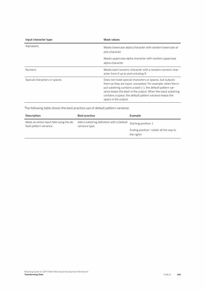
Input character type Mask values
Alphabetic Masks lowercase alpha character with random lowercase alpha character
Masks uppercase alpha character with random uppercase alpha character
Numeric Masks each numeric character with a random numeric character from 0 up to and including 9.
Special characters or spaces Does not mask special characters or spaces, but outputs them as they are input, unmasked. For example, when the input substring contains a dash (-), the default pattern variance keeps the dash in the output. When the input substring contains a space, the default pattern variance keeps the space in the output.
The following table shows the best practice use of default pattern variance:
Description Best practice Example
Mask an entire input field using the default pattern variance.
Add a substring definition with a Default variance type.
Starting position: 1
Ending position: <slider all the way to the right>
Modeling Guide for SAP HANA Web-based Development WorkbenchTransforming Data PUBLIC 145
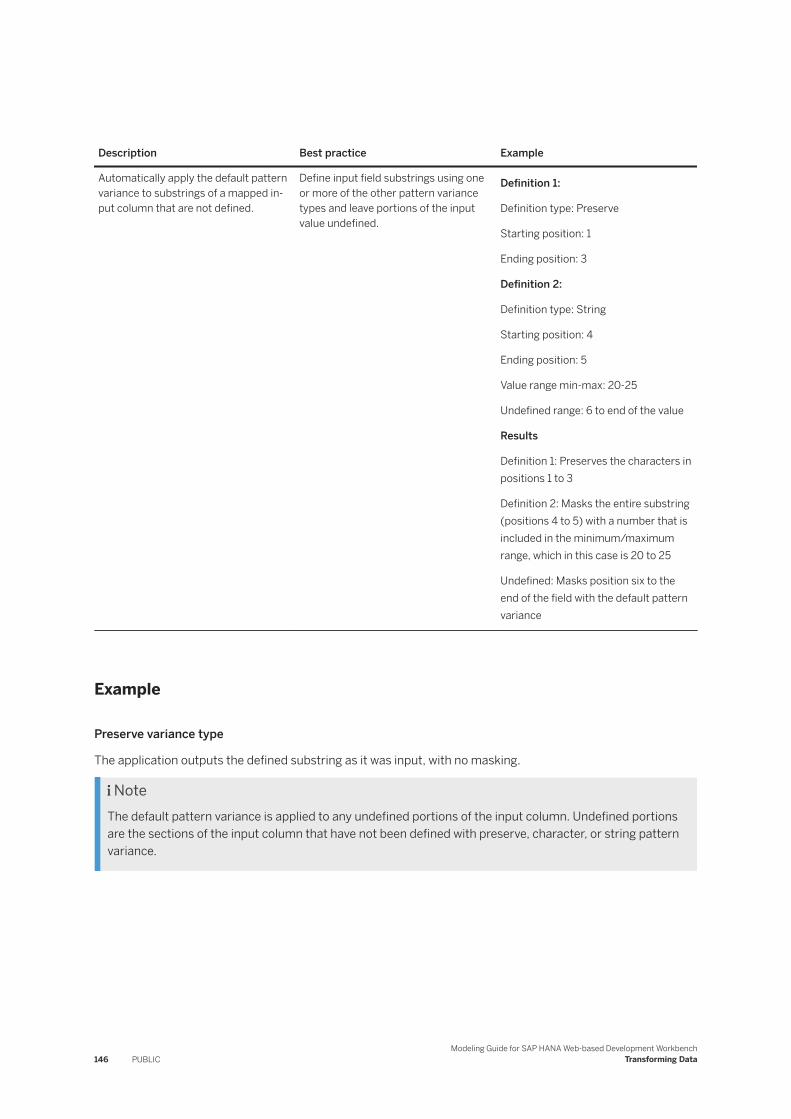
Description Best practice Example
Automatically apply the default pattern variance to substrings of a mapped input column that are not defined.
Define input field substrings using one or more of the other pattern variance types and leave portions of the input value undefined.
Definition 1:
Definition type: Preserve
Starting position: 1
Ending position: 3
Definition 2:
Definition type: String
Starting position: 4
Ending position: 5
Value range min-max: 20-25
Undefined range: 6 to end of the value
Results
Definition 1: Preserves the characters in positions 1 to 3
Definition 2: Masks the entire substring (positions 4 to 5) with a number that is included in the minimum/maximum range, which in this case is 20 to 25
Undefined: Masks position six to the end of the field with the default pattern variance
Example
Preserve variance type
The application outputs the defined substring as it was input, with no masking.
NoteThe default pattern variance is applied to any undefined portions of the input column. Undefined portions are the sections of the input column that have not been defined with preserve, character, or string pattern variance.
146 PUBLICModeling Guide for SAP HANA Web-based Development Workbench
Transforming Data
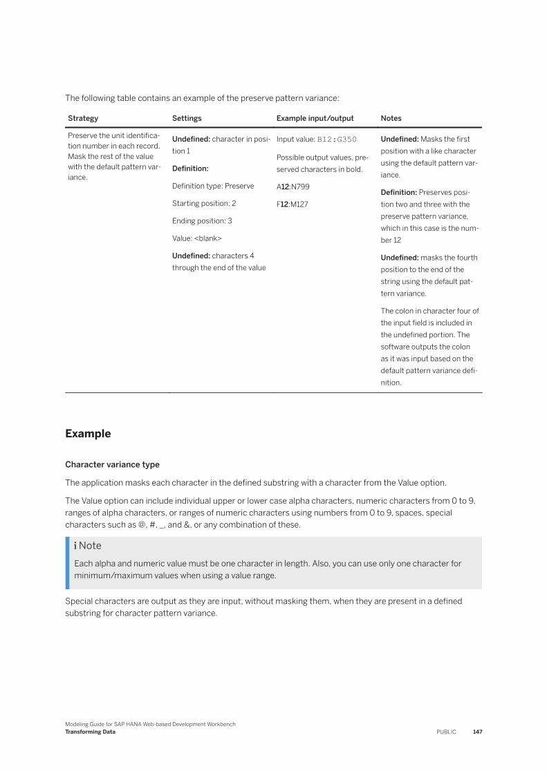
The following table contains an example of the preserve pattern variance:
Strategy Settings Example input/output Notes
Preserve the unit identifica-tion number in each record. Mask the rest of the value with the default pattern variance.
Undefined: character in position 1
Definition:
Definition type: Preserve
Starting position: 2
Ending position: 3
Value: <blank>
Undefined: characters 4 through the end of the value
Input value: B12:G350
Possible output values, preserved characters in bold.
A12:N799
F12:M127
Undefined: Masks the first position with a like character using the default pattern variance.
Definition: Preserves position two and three with the preserve pattern variance, which in this case is the number 12
Undefined: masks the fourth position to the end of the string using the default pattern variance.
The colon in character four of the input field is included in the undefined portion. The software outputs the colon as it was input based on the default pattern variance defi-nition.
Example
Character variance type
The application masks each character in the defined substring with a character from the Value option.
The Value option can include individual upper or lower case alpha characters, numeric characters from 0 to 9, ranges of alpha characters, or ranges of numeric characters using numbers from 0 to 9, spaces, special characters such as @, #, _, and &, or any combination of these.
NoteEach alpha and numeric value must be one character in length. Also, you can use only one character for minimum/maximum values when using a value range.
Special characters are output as they are input, without masking them, when they are present in a defined substring for character pattern variance.
Modeling Guide for SAP HANA Web-based Development WorkbenchTransforming Data PUBLIC 147
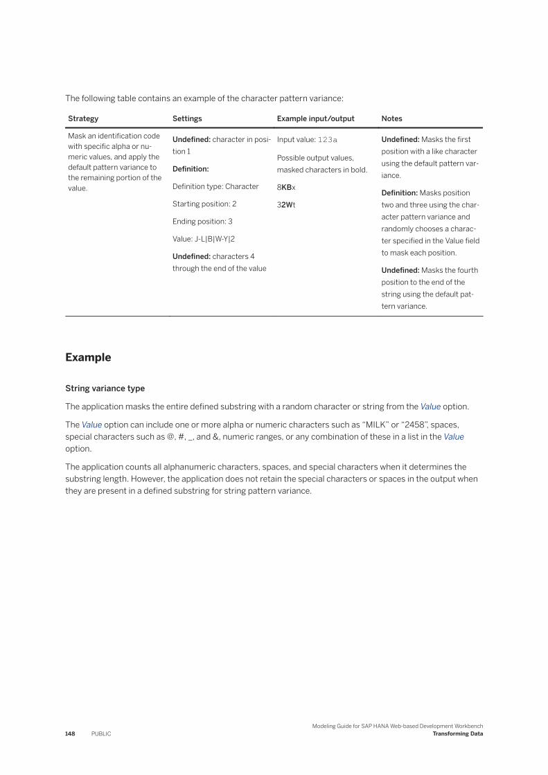
The following table contains an example of the character pattern variance:
Strategy Settings Example input/output Notes
Mask an identification code with specific alpha or numeric values, and apply the default pattern variance to the remaining portion of the value.
Undefined: character in position 1
Definition:
Definition type: Character
Starting position: 2
Ending position: 3
Value: J-L|B|W-Y|2
Undefined: characters 4 through the end of the value
Input value: 123a
Possible output values, masked characters in bold.
8KBx
32Wt
Undefined: Masks the first position with a like character using the default pattern variance.
Definition: Masks position two and three using the character pattern variance and randomly chooses a character specified in the Value field to mask each position.
Undefined: Masks the fourth position to the end of the string using the default pattern variance.
Example
String variance type
The application masks the entire defined substring with a random character or string from the Value option.
The Value option can include one or more alpha or numeric characters such as “MILK” or “2458”, spaces, special characters such as @, #, _, and &, numeric ranges, or any combination of these in a list in the Value option.
The application counts all alphanumeric characters, spaces, and special characters when it determines the substring length. However, the application does not retain the special characters or spaces in the output when they are present in a defined substring for string pattern variance.
148 PUBLICModeling Guide for SAP HANA Web-based Development Workbench
Transforming Data
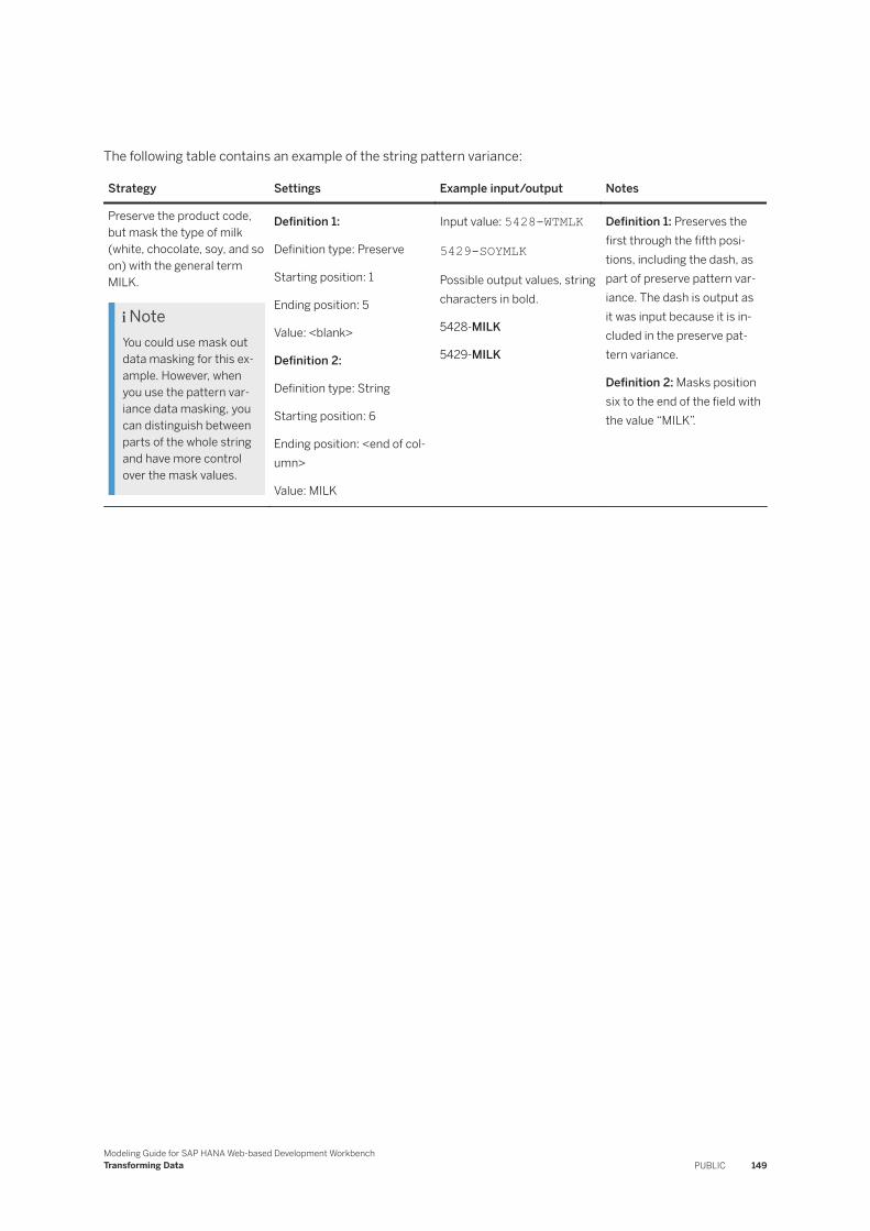
The following table contains an example of the string pattern variance:
Strategy Settings Example input/output Notes
Preserve the product code, but mask the type of milk (white, chocolate, soy, and so on) with the general term MILK.
NoteYou could use mask out data masking for this example. However, when you use the pattern variance data masking, you can distinguish between parts of the whole string and have more control over the mask values.
Definition 1:
Definition type: Preserve
Starting position: 1
Ending position: 5
Value: <blank>
Definition 2:
Definition type: String
Starting position: 6
Ending position: <end of column>
Value: MILK
Input value: 5428-WTMLK
5429-SOYMLK
Possible output values, string characters in bold.
5428-MILK
5429-MILK
Definition 1: Preserves the first through the fifth positions, including the dash, as part of preserve pattern variance. The dash is output as it was input because it is included in the preserve pattern variance.
Definition 2: Masks position six to the end of the field with the value “MILK”.
Modeling Guide for SAP HANA Web-based Development WorkbenchTransforming Data PUBLIC 149
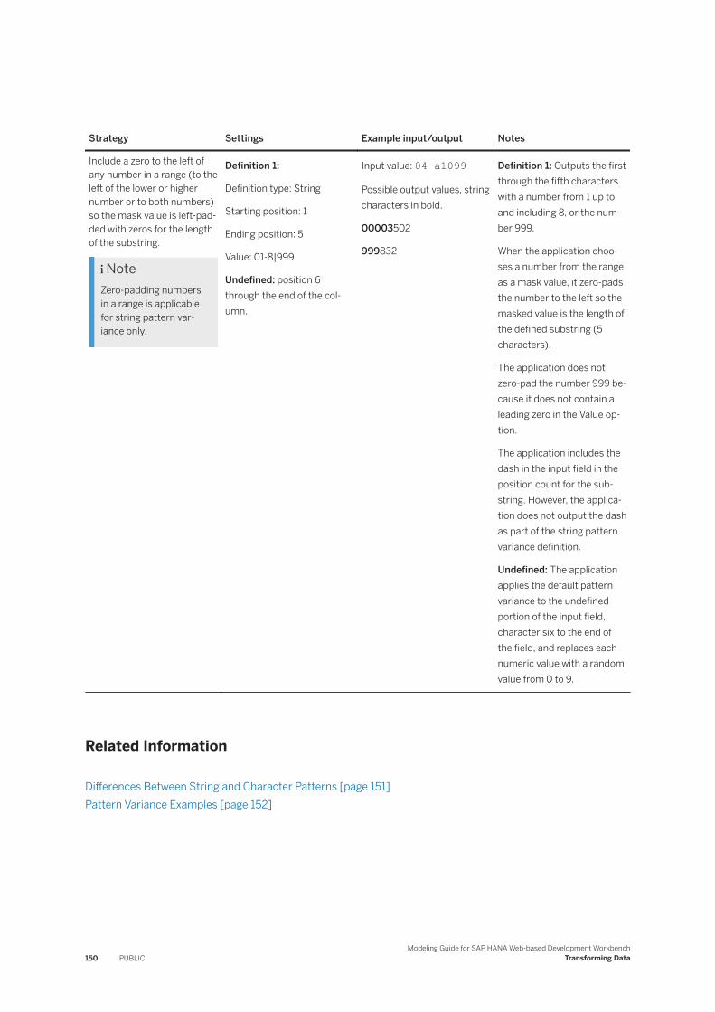
Strategy Settings Example input/output Notes
Include a zero to the left of any number in a range (to the left of the lower or higher number or to both numbers) so the mask value is left-padded with zeros for the length of the substring.
NoteZero-padding numbers in a range is applicable for string pattern variance only.
Definition 1:
Definition type: String
Starting position: 1
Ending position: 5
Value: 01-8|999
Undefined: position 6 through the end of the column.
Input value: 04-a1099
Possible output values, string characters in bold.
00003502
999832
Definition 1: Outputs the first through the fifth characters with a number from 1 up to and including 8, or the number 999.
When the application chooses a number from the range as a mask value, it zero-pads the number to the left so the masked value is the length of the defined substring (5 characters).
The application does not zero-pad the number 999 because it does not contain a leading zero in the Value option.
The application includes the dash in the input field in the position count for the substring. However, the application does not output the dash as part of the string pattern variance definition.
Undefined: The application applies the default pattern variance to the undefined portion of the input field, character six to the end of the field, and replaces each numeric value with a random value from 0 to 9.
Related Information
Differences Between String and Character Patterns [page 151]Pattern Variance Examples [page 152]
150 PUBLICModeling Guide for SAP HANA Web-based Development Workbench
Transforming Data
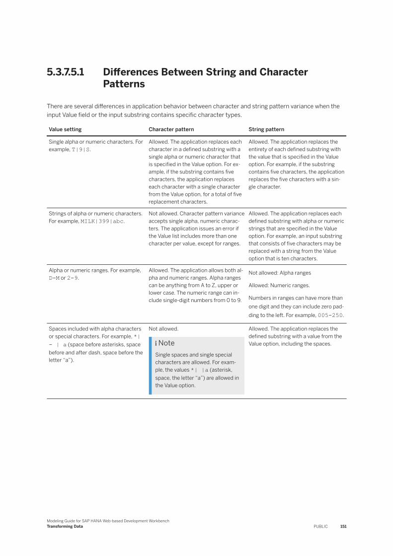
5.3.7.5.1 Differences Between String and Character Patterns
There are several differences in application behavior between character and string pattern variance when the input Value field or the input substring contains specific character types.
Value setting Character pattern String pattern
Single alpha or numeric characters. For example, T|9|S.
Allowed. The application replaces each character in a defined substring with a single alpha or numeric character that is specified in the Value option. For example, if the substring contains five characters, the application replaces each character with a single character from the Value option, for a total of five replacement characters.
Allowed. The application replaces the entirety of each defined substring with the value that is specified in the Value option. For example, if the substring contains five characters, the application replaces the five characters with a single character.
Strings of alpha or numeric characters. For example, MILK|399|abc.
Not allowed. Character pattern variance accepts single alpha, numeric characters. The application issues an error if the Value list includes more than one character per value, except for ranges.
Allowed. The application replaces each defined substring with alpha or numeric strings that are specified in the Value option. For example, an input substring that consists of five characters may be replaced with a string from the Value option that is ten characters.
Alpha or numeric ranges. For example, D-M or 2-9.
Allowed. The application allows both alpha and numeric ranges. Alpha ranges can be anything from A to Z, upper or lower case. The numeric range can include single-digit numbers from 0 to 9.
Not allowed: Alpha ranges
Allowed: Numeric ranges.
Numbers in ranges can have more than one digit and they can include zero padding to the left. For example, 005-250.
Spaces included with alpha characters or special characters. For example, *| - | a (space before asterisks, space before and after dash, space before the letter “a”).
Not allowed.
NoteSingle spaces and single special characters are allowed. For example, the values *| |a (asterisk, space, the letter “a”) are allowed in the Value option.
Allowed. The application replaces the defined substring with a value from the Value option, including the spaces.
Modeling Guide for SAP HANA Web-based Development WorkbenchTransforming Data PUBLIC 151
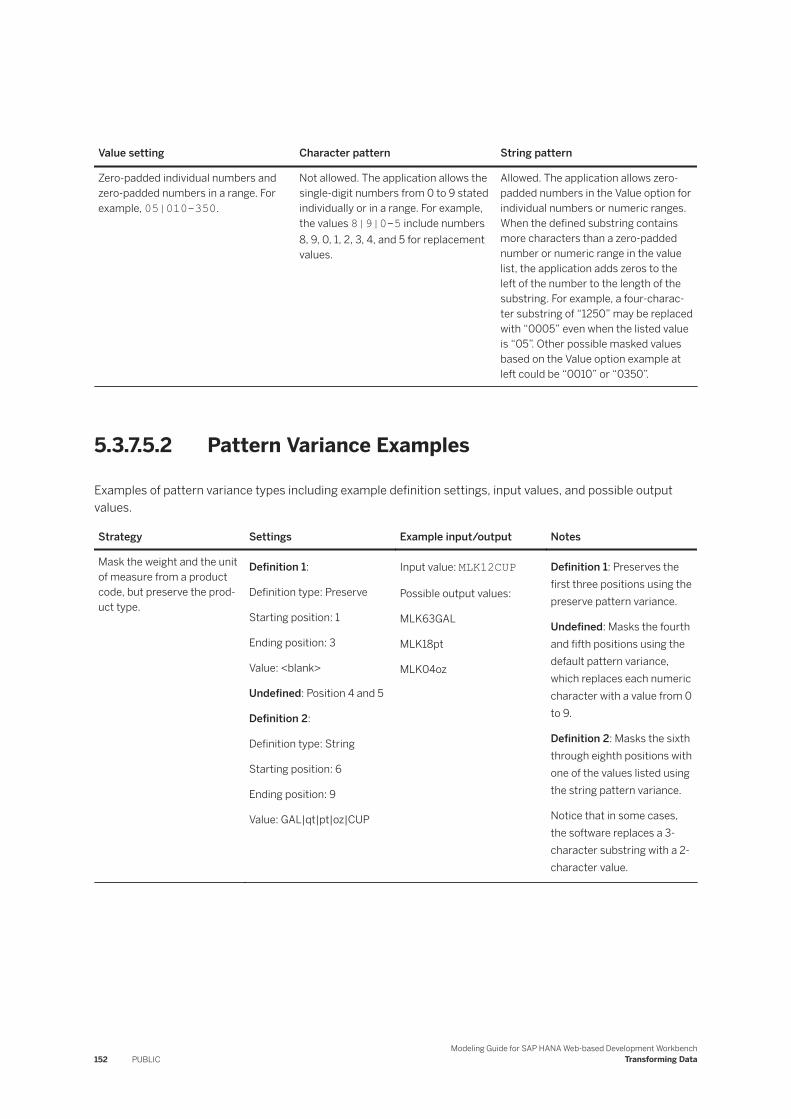
Value setting Character pattern String pattern
Zero-padded individual numbers and zero-padded numbers in a range. For example, 05|010-350.
Not allowed. The application allows the single-digit numbers from 0 to 9 stated individually or in a range. For example, the values 8|9|0-5 include numbers 8, 9, 0, 1, 2, 3, 4, and 5 for replacement values.
Allowed. The application allows zero-padded numbers in the Value option for individual numbers or numeric ranges. When the defined substring contains more characters than a zero-padded number or numeric range in the value list, the application adds zeros to the left of the number to the length of the substring. For example, a four-character substring of “1250” may be replaced with “0005” even when the listed value is “05”. Other possible masked values based on the Value option example at left could be “0010” or “0350”.
5.3.7.5.2 Pattern Variance Examples
Examples of pattern variance types including example definition settings, input values, and possible output values.
Strategy Settings Example input/output Notes
Mask the weight and the unit of measure from a product code, but preserve the product type.
Definition 1:
Definition type: Preserve
Starting position: 1
Ending position: 3
Value: <blank>
Undefined: Position 4 and 5
Definition 2:
Definition type: String
Starting position: 6
Ending position: 9
Value: GAL|qt|pt|oz|CUP
Input value: MLK12CUP
Possible output values:
MLK63GAL
MLK18pt
MLK04oz
Definition 1: Preserves the first three positions using the preserve pattern variance.
Undefined: Masks the fourth and fifth positions using the default pattern variance, which replaces each numeric character with a value from 0 to 9.
Definition 2: Masks the sixth through eighth positions with one of the values listed using the string pattern variance.
Notice that in some cases, the software replaces a 3-character substring with a 2-character value.
152 PUBLICModeling Guide for SAP HANA Web-based Development Workbench
Transforming Data
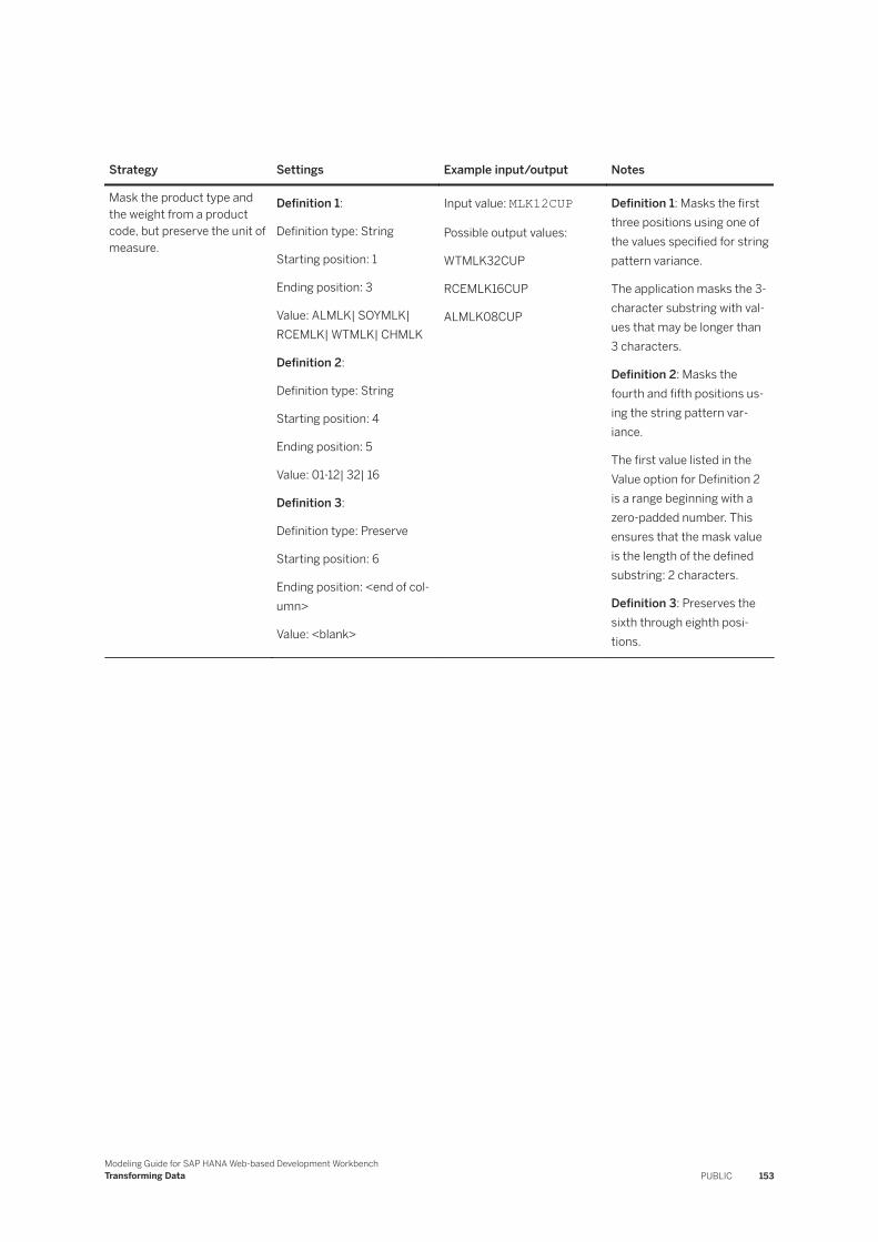
Strategy Settings Example input/output Notes
Mask the product type and the weight from a product code, but preserve the unit of measure.
Definition 1:
Definition type: String
Starting position: 1
Ending position: 3
Value: ALMLK| SOYMLK| RCEMLK| WTMLK| CHMLK
Definition 2:
Definition type: String
Starting position: 4
Ending position: 5
Value: 01-12| 32| 16
Definition 3:
Definition type: Preserve
Starting position: 6
Ending position: <end of column>
Value: <blank>
Input value: MLK12CUP
Possible output values:
WTMLK32CUP
RCEMLK16CUP
ALMLK08CUP
Definition 1: Masks the first three positions using one of the values specified for string pattern variance.
The application masks the 3-character substring with values that may be longer than 3 characters.
Definition 2: Masks the fourth and fifth positions using the string pattern variance.
The first value listed in the Value option for Definition 2 is a range beginning with a zero-padded number. This ensures that the mask value is the length of the defined substring: 2 characters.
Definition 3: Preserves the sixth through eighth positions.
Modeling Guide for SAP HANA Web-based Development WorkbenchTransforming Data PUBLIC 153

Strategy Settings Example input/output Notes
Mask the number of paper sheets per package, and the type of packaging from the product description column.
Definition 1:
Definition type: Character
Starting position: 1
Ending position: 4
Value: 0-9
Undefined: Position 5
Definition 2:
Definition type: String
Starting position: 6
Ending position: <end of column>
Value: Ream| Case| Pack| Box
Input value: 1500/Ream
Possible output values:
0950/Case
8945/Box
2639/Pack
Definition 1: Masks the first through fourth positions with a number from 0 to 9.
The user could leave the first through fifth positions undefined so the application masks the substring using the default pattern variance to get similar output values. The forward slash would be output as part of the substring in this case.
Undefined: Outputs the forward slash (/) character in the fifth position using the default pattern variance, which maintains special characters on output.
Definition 2: Mask the sixth position to the end of the column with one of the character strings listed in the Value option.
154 PUBLICModeling Guide for SAP HANA Web-based Development Workbench
Transforming Data
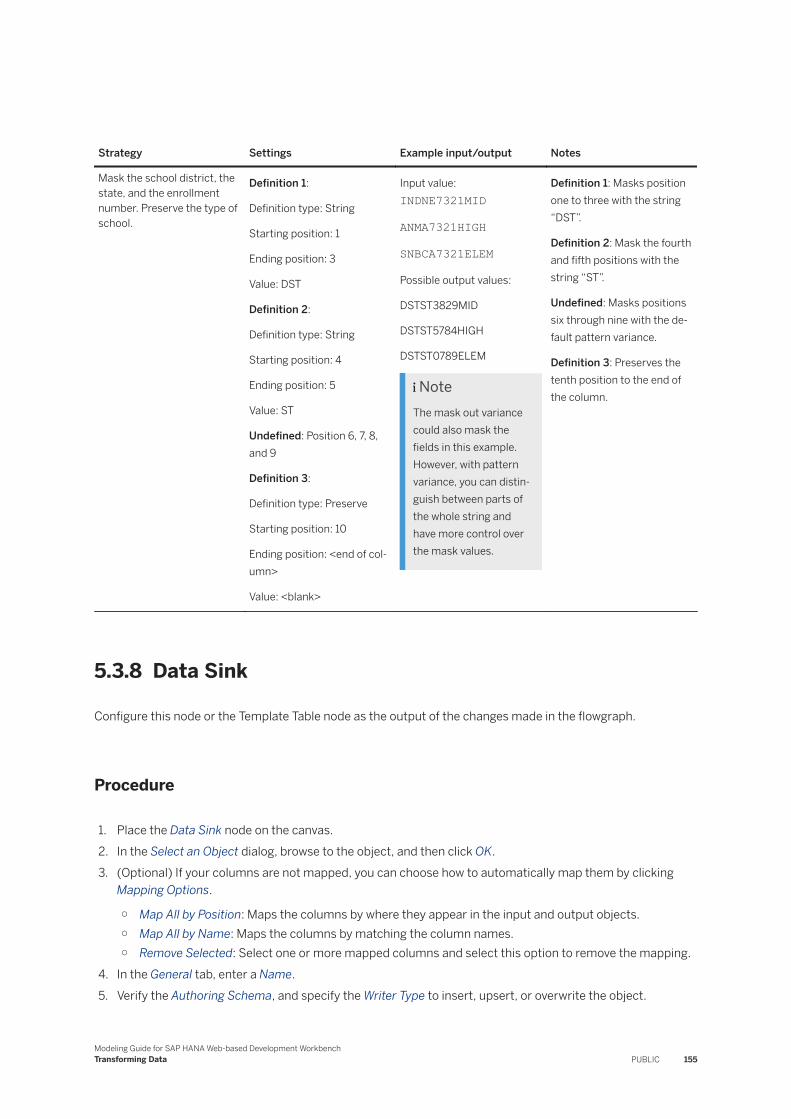
Strategy Settings Example input/output Notes
Mask the school district, the state, and the enrollment number. Preserve the type of school.
Definition 1:
Definition type: String
Starting position: 1
Ending position: 3
Value: DST
Definition 2:
Definition type: String
Starting position: 4
Ending position: 5
Value: ST
Undefined: Position 6, 7, 8, and 9
Definition 3:
Definition type: Preserve
Starting position: 10
Ending position: <end of column>
Value: <blank>
Input value: INDNE7321MID
ANMA7321HIGH
SNBCA7321ELEM
Possible output values:
DSTST3829MID
DSTST5784HIGH
DSTST0789ELEM
NoteThe mask out variance could also mask the fields in this example. However, with pattern variance, you can distinguish between parts of the whole string and have more control over the mask values.
Definition 1: Masks position one to three with the string “DST”.
Definition 2: Mask the fourth and fifth positions with the string “ST”.
Undefined: Masks positions six through nine with the default pattern variance.
Definition 3: Preserves the tenth position to the end of the column.
5.3.8 Data Sink
Configure this node or the Template Table node as the output of the changes made in the flowgraph.
Procedure
1. Place the Data Sink node on the canvas.2. In the Select an Object dialog, browse to the object, and then click OK.3. (Optional) If your columns are not mapped, you can choose how to automatically map them by clicking
Mapping Options.
○ Map All by Position: Maps the columns by where they appear in the input and output objects.○ Map All by Name: Maps the columns by matching the column names.○ Remove Selected: Select one or more mapped columns and select this option to remove the mapping.
4. In the General tab, enter a Name.5. Verify the Authoring Schema, and specify the Writer Type to insert, upsert, or overwrite the object.
Modeling Guide for SAP HANA Web-based Development WorkbenchTransforming Data PUBLIC 155
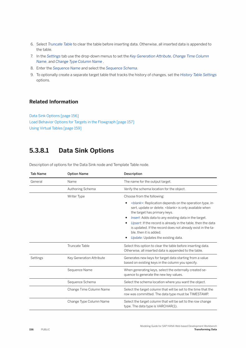
6. Select Truncate Table to clear the table before inserting data. Otherwise, all inserted data is appended to the table.
7. In the Settings tab use the drop-down menus to set the Key Generation Attribute, Change Time Column Name, and Change Type Column Name .
8. Enter the Sequence Name and select the Sequence Schema.9. To optionally create a separate target table that tracks the history of changes, set the History Table Settings
options.
Related Information
Data Sink Options [page 156]Load Behavior Options for Targets in the Flowgraph [page 157]Using Virtual Tables [page 159]
5.3.8.1 Data Sink Options
Description of options for the Data Sink node and Template Table node.
Tab Name Option Name Description
General Name The name for the output target.
Authoring Schema Verify the schema location for the object.
Writer Type Choose from the following:
● <blank>: Replication depends on the operation type, insert, update or delete. <blank> is only available when the target has primary keys.
● Insert: Adds data to any existing data in the target.● Upsert: If the record is already in the table, then the data
is updated. If the record does not already exist in the table, then it is added.
● Update: Updates the existing data.
Truncate Table Select this option to clear the table before inserting data. Otherwise, all inserted data is appended to the table.
Settings Key Generation Attribute Generates new keys for target data starting from a value based on existing keys in the column you specify.
Sequence Name When generating keys, select the externally created sequence to generate the new key values.
Sequence Schema Select the schema location where you want the object.
Change Time Column Name Select the target column that will be set to the time that the row was committed. The data type must be TIMESTAMP.
Change Type Column Name Select the target column that will be set to the row change type. The data type is VARCHAR(1).
156 PUBLICModeling Guide for SAP HANA Web-based Development Workbench
Transforming Data

Tab Name Option Name Description
History Table Settings Schema Name (Optional) Select the schema location where you want the history table.
Name Enter a name for the history table.
Type Select whether the target is a database table or a template table.
Data Layout Specify whether to load the output data in columns or rows.
5.3.8.2 Load Behavior Options for Targets in the Flowgraph
For flowgraphs, you can select options that enable different target-loading behaviors and include columns that display the time and type of change made in the source.
Context
Simple replication of a source table to a target table results in a copy of the source with the same row count and columns. However, because this process also includes information on what row has changed and when, you can add these change types and change times to the target table.
For example, in simple replication, deleted rows do not display in the target table. To display the rows that were deleted, you can select UPSERT when loading the target. The deleted rows display with a change type of D.
You could also choose to display all changes to the target using INSERT functionality, which provides a change log table. Every changed row would be inserted into the target table and you can include columns that display the change types and change times.
Modeling Guide for SAP HANA Web-based Development WorkbenchTransforming Data PUBLIC 157
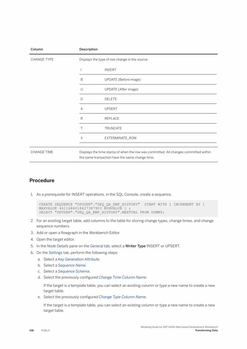
Column Description
CHANGE TYPE Displays the type of row change in the source:
I INSERT
B UPDATE (Before image)
U UPDATE (After image)
D DELETE
A UPSERT
R REPLACE
T TRUNCATE
X EXTERMINATE_ROW
CHANGE TIME Displays the time stamp of when the row was committed. All changes committed within the same transaction have the same change time.
Procedure
1. As a prerequisite for INSERT operations, in the SQL Console, create a sequence.
CREATE SEQUENCE "DPUSER"."SEQ_QA_EMP_HISTORY" START WITH 1 INCREMENT BY 1 MAXVALUE 4611686018427387903 MINVALUE 1 ; SELECT "DPUSER"."SEQ_QA_EMP_HISTORY".NEXTVAL FROM DUMMY;
2. For an existing target table, add columns to the table for storing change types, change times, and change sequence numbers.
3. Add or open a flowgraph in the Workbench Editor.4. Open the target editor.5. In the Node Details pane on the General tab, select a Writer Type INSERT or UPSERT.6. On the Settings tab, perform the following steps:
a. Select a Key Generation Attribute.b. Select a Sequence Name.c. Select a Sequence Schema.d. Select the previously configured Change Time Column Name.
If the target is a template table, you can select an existing column or type a new name to create a new target table.
e. Select the previously configured Change Type Column Name.
If the target is a template table, you can select an existing column or type a new name to create a new target table.
158 PUBLICModeling Guide for SAP HANA Web-based Development Workbench
Transforming Data
7. Save the flowgraph.8. Activate the flowgraph.
Related Information
Load Behavior Options for Targets in Replication Tasks [page 26]
5.3.8.3 Using Virtual Tables
You can write to virtual tables within a data sink for some adapters.
The following adapters support writing to virtual tables:
● Log Reader● File● SAP HANA● SAP ASE● Teradata● IBM DB2 for z/OS Adapter
The process of writing to virtual tables is generally the same as writing to SAP HANA tables. For example, in the configuration of the Data Sink node, you can choose in the Writer Type option to insert, upsert, or update the new records in the target table.
5.3.9 Data Source
Edit nodes that represent data sources.
Procedure
1. Place the Data Source node onto the canvas.
To preview the existing data in the table or view, click the magnifying glass icon.2. In the Select an Object dialog, type the name of the object to add, or browse the object tree to select one or
more objects, and click OK.3. In the General tab, verify the object Type (database or template table) and Catalog Object schema and
name.4. (Optional) Select Real-time behavior to run the flowgraph whenever the source object is updated. You can
also select with Schema Change to track the addition and deletion of columns in the primary database tables. These options are available when the data source object is a virtual table.
Modeling Guide for SAP HANA Web-based Development WorkbenchTransforming Data PUBLIC 159

NoteIf a column is added or deleted in the source, selecting with Schema Change does not add or delete that column in the target.
5. (Optional) Select the Partitions tab to partition the object. Partitioned objects can enhance the performance and can make the large data sets more manageable.a. Choose Range or List.b. In the Attribute option, choose the column that you want to use as the base of your partitioning. You
will set your partitions based on the data in this column.c. Click the + icon and enter the partition Name and Value.
You must create a minimum of two partitions. The Value of the last partition should always be blank so that it captures any records that do not meet the partition criteria.
d. When you have finished adding partitions, click Back.6. Click Save to return to the flowgraph.
Related Information
Reconcile Changes in the Source [page 160]Propagation of Source Schema Changes [page 161]Data Source Options [page 163]Reading from Virtual Tables [page 164]
5.3.9.1 Reconcile Changes in the Source
In the Data Source node in a flowgraph, you reconcile differences that have occurred between the source table and its current structure in the node.
Context
When the structure of an underlying object such as a SAP HANA table, virtual table, and so on, for a Data Source changes, you can view and update what has changed in the structure since adding the Data Source to the flowgraph.
Procedure
1. View the flowgraph containing the Data Source node.2. Select the Compare Tables icon next to the data source.
160 PUBLICModeling Guide for SAP HANA Web-based Development Workbench
Transforming Data
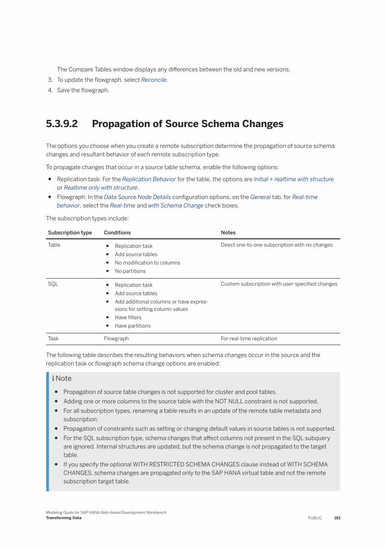
The Compare Tables window displays any differences between the old and new versions.3. To update the flowgraph, select Reconcile.4. Save the flowgraph.
5.3.9.2 Propagation of Source Schema Changes
The options you choose when you create a remote subscription determine the propagation of source schema changes and resultant behavior of each remote subscription type.
To propagate changes that occur in a source table schema, enable the following options:
● Replication task: For the Replication Behavior for the table, the options are Initial + realtime with structure or Realtime only with structure.
● Flowgraph: In the Data Source Node Details configuration options, on the General tab, for Real-time behavior, select the Real-time and with Schema Change check boxes.
The subscription types include:
Subscription type Conditions Notes
Table ● Replication task● Add source tables● No modification to columns● No partitions
Direct one-to-one subscription with no changes
SQL ● Replication task● Add source tables● Add additional columns or have expres
sions for setting column values● Have filters● Have partitions
Custom subscription with user-specified changes
Task Flowgraph For real-time replication
The following table describes the resulting behaviors when schema changes occur in the source and the replication task or flowgraph schema change options are enabled:
Note● Propagation of source table changes is not supported for cluster and pool tables.● Adding one or more columns to the source table with the NOT NULL constraint is not supported.● For all subscription types, renaming a table results in an update of the remote table metadata and
subscription.● Propagation of constraints such as setting or changing default values in source tables is not supported.● For the SQL subscription type, schema changes that affect columns not present in the SQL subquery
are ignored. Internal structures are updated, but the schema change is not propagated to the target table.
● If you specify the optional WITH RESTRICTED SCHEMA CHANGES clause instead of WITH SCHEMA CHANGES, schema changes are propagated only to the SAP HANA virtual table and not the remote subscription target table.
Modeling Guide for SAP HANA Web-based Development WorkbenchTransforming Data PUBLIC 161
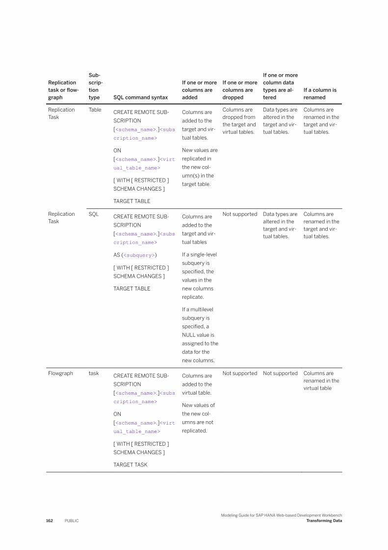
Replication task or flowgraph
Subscription type SQL command syntax
If one or more columns are added
If one or more columns are dropped
If one or more column data types are altered
If a column is renamed
Replication Task
Table CREATE REMOTE SUBSCRIPTION [<schema_name>.]<subscription_name>
ON [<schema_name>.]<virtual_table_name>
[ WITH [ RESTRICTED ] SCHEMA CHANGES ]
TARGET TABLE
Columns are added to the target and virtual tables.
New values are replicated in the new column(s) in the target table.
Columns are dropped from the target and virtual tables.
Data types are altered in the target and virtual tables.
Columns are renamed in the target and virtual tables.
Replication Task
SQL CREATE REMOTE SUBSCRIPTION [<schema_name>.]<subscription_name>
AS (<subquery>)
[ WITH [ RESTRICTED ] SCHEMA CHANGES ]
TARGET TABLE
Columns are added to the target and virtual tables
If a single-level subquery is specified, the values in the new columns replicate.
If a multilevel subquery is specified, a NULL value is assigned to the data for the new columns.
Not supported Data types are altered in the target and virtual tables.
Columns are renamed in the target and virtual tables.
Flowgraph task CREATE REMOTE SUBSCRIPTION [<schema_name>.]<subscription_name>
ON [<schema_name>.]<virtual_table_name>
[ WITH [ RESTRICTED ] SCHEMA CHANGES ]
TARGET TASK
Columns are added to the virtual table.
New values of the new columns are not replicated.
Not supported Not supported Columns are renamed in the virtual table
162 PUBLICModeling Guide for SAP HANA Web-based Development Workbench
Transforming Data
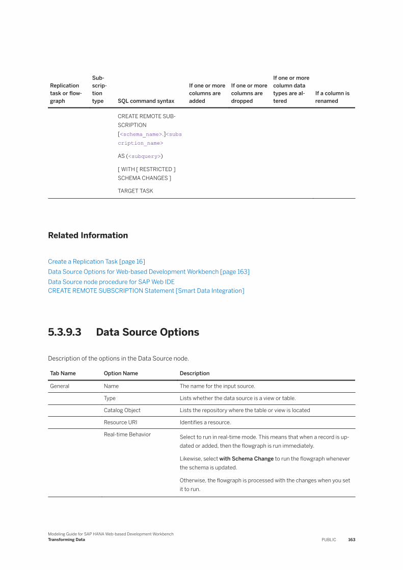
Replication task or flowgraph
Subscription type SQL command syntax
If one or more columns are added
If one or more columns are dropped
If one or more column data types are altered
If a column is renamed
CREATE REMOTE SUBSCRIPTION [<schema_name>.]<subscription_name>
AS (<subquery>)
[ WITH [ RESTRICTED ] SCHEMA CHANGES ]
TARGET TASK
Related Information
Create a Replication Task [page 16]Data Source Options for Web-based Development Workbench [page 163]Data Source node procedure for SAP Web IDECREATE REMOTE SUBSCRIPTION Statement [Smart Data Integration]
5.3.9.3 Data Source Options
Description of the options in the Data Source node.
Tab Name Option Name Description
General Name The name for the input source.
Type Lists whether the data source is a view or table.
Catalog Object Lists the repository where the table or view is located
Resource URI Identifies a resource.
Real-time Behavior Select to run in real-time mode. This means that when a record is updated or added, then the flowgraph is run immediately.
Likewise, select with Schema Change to run the flowgraph whenever the schema is updated.
Otherwise, the flowgraph is processed with the changes when you set it to run.
Modeling Guide for SAP HANA Web-based Development WorkbenchTransforming Data PUBLIC 163
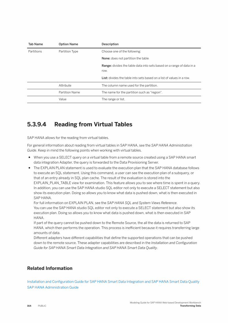
Tab Name Option Name Description
Partitions Partition Type Choose one of the following:
None: does not partition the table
Range: divides the table data into sets based on a range of data in a row.
List: divides the table into sets based on a list of values in a row.
Attribute The column name used for the partition.
Partition Name The name for the partition such as "region".
Value The range or list.
5.3.9.4 Reading from Virtual Tables
SAP HANA allows for the reading from virtual tables.
For general information about reading from virtual tables in SAP HANA, see the SAP HANA Administration Guide. Keep in mind the following points when working with virtual tables.
● When you use a SELECT query on a virtual table from a remote source created using a SAP HANA smart data integration Adapter, the query is forwarded to the Data Provisioning Server.
● The EXPLAIN PLAN statement is used to evaluate the execution plan that the SAP HANA database follows to execute an SQL statement. Using this command, a user can see the execution plan of a subquery, or that of an entry already in SQL plan cache. The result of the evaluation is stored into the EXPLAIN_PLAN_TABLE view for examination. This feature allows you to see where time is spent in a query.In addition, you can use the SAP HANA studio SQL editor not only to execute a SELECT statement but also show its execution plan. Doing so allows you to know what data is pushed down, what is then executed in SAP HANA.For full information on EXPLAIN PLAN, see the SAP HANA SQL and System Views Reference.You can use the SAP HANA studio SQL editor not only to execute a SELECT statement but also show its execution plan. Doing so allows you to know what data is pushed down, what is then executed in SAP HANA.If part of the query cannot be pushed down to the Remote Source, the all the data is returned to SAP HANA, which then performs the operation. This process is inefficient because it requires transferring large amounts of data.Different adapters have different capabilities that define the supported operations that can be pushed down to the remote source. These adapter capabilities are described in the Installation and Configuration Guide for SAP HANA Smart Data Integration and SAP HANA Smart Data Quality.
Related Information
Installation and Configuration Guide for SAP HANA Smart Data Integration and SAP HANA Smart Data QualitySAP HANA Administration Guide
164 PUBLICModeling Guide for SAP HANA Web-based Development Workbench
Transforming Data

SAP HANA SQL and System Views Reference
5.3.10 Date Generator
Creates one column that contains a generated date.
Context
NoteThe Date Generation node is not available for real-time processing.
After the node is placed on the canvas, you can see the Inspect icon. This icon opens a quick view that provides a summary of the node. The information available in the quick view depends on whether the node is connected to other nodes and how the node is configured.
After the node is connected and configured, you can see this information in the quick view when available.
Icon Description
Output Columns Shows the number of output columns.
Set the following options.
Procedure
1. Enter a Name for the node.2. In the Start Date option, enter the first date to be generated.3. In the End Date option, enter the last date to be generated.4. In the Date Increment option, select an interval for which the dates should be generated, then click OK.
Modeling Guide for SAP HANA Web-based Development WorkbenchTransforming Data PUBLIC 165
5.3.11 Filter
A Filter node represents a relational selection combined with a projection operation. It also allows calculated attributes to be added to the output.
Procedure
1. Drag the Filter node onto the canvas, and connect the source data or the previous node to the Filter node. Double-click the node to view the settings.
2. (Optional) Select JIT Data Preview to create a preview of the data as it would be output up to this point in the flowgraph. All transformations from previous nodes, including the changes set in this node are shown in the preview by clicking the Data Preview icon on the canvas next to this node.
3. (Optional) Select Distinct to output only unique records.4. (Optional) To copy any columns that are not already mapped to the output target, drag them from the
Input pane to the Output pane. You may also remove any output columns by clicking the pencil icon or the trash icon, respectively. You can multi-select the columns that you do not want output by using the CTRL or Shift key, and then Delete.
5. (Optional) Click Load Elements & Functions to populate the Expression Editor. Drag input columns into the Mapping tab to define the output mapping and perform some sort of calculation. Choose the functions and the operators. For example, you might want to calculate the workdays in a quarter, so you would use the Workdays_Between function in an expression like this: WORKDAYS_BETWEEN (<factory_calendar_id>, <start_date>, <end_date> [, <source_schema>]). Click Validate Syntax to ensure that the expression is valid.
6. Click the Filter node tab and then click Load Elements & Functions to populate the Expression Editor. You can use the Expression Editor or type an expression to filter the data from the input to the output. Drag the input columns, select a function and the operators. For example, if you want to move all the records that are in Canada for the year 2017, your filter might look like this: "Filter1_input"."COUNTRY" = "Canada" AND "Filter1_input"."DATE"="2017". See the "SQL Functions" topic in the SAP HANA SQL and System Views Reference for more information about each function.
7. Click Back to return to the flowgraph.
Related Information
Filter Options [page 167]
166 PUBLICModeling Guide for SAP HANA Web-based Development Workbench
Transforming Data
5.3.11.1 Filter Options
Description of options for the Filter node.
Tab Option Description
Mapping and Filter Node
JIT Data Preview Creates a preview of the data as it would be output up to this point in the flowgraph. All transformations from previous nodes, including the changes set in this node are shown in the preview by clicking the Data Preview icon on the canvas next to this node
Mapping and Filter Node
Distinct (Optional). Select to output only unique records. The records must match exactly. If you know that you have duplicates, but have a ROW_ID column, or another column that has a unique identifier for each record, then you will want to suppress that column in the Filter node.
Mapping and Filter Node
Load Elements & Functions Populates the options in the Expression Editor.
Mapping Validate Syntax Checks that the expression is valid.
5.3.12 Geocode
Generates latitude and longitude coordinates for an address, and generates addresses from latitude and longitude coordinates.
The Geocode node assigns geographic location data.
Only one input source is allowed.
NoteThe Geocode node is available for real-time processing.
NoteYou can use the SAP HANA smart data quality Geocode technology in SAP HANA spatial to assign geographic coordinates without having to create a workflow or use a third party geocoding provider. For details, see the SAP HANA Spatial Reference.
Types of Geocoding
There are two types of geocoding you can select, depending on the type of information available in your input data. The first type is based on address data. When the Geocode Configuration window opens, select Address. This option takes the address and assigns latitude and longitude coordinates to the output data.
The second type occurs when your input data already contains the latitude and longitude coordinates, and assigns an address based on those coordinates. When the Geocode Configuration window opens, select Coordinates.
Modeling Guide for SAP HANA Web-based Development WorkbenchTransforming Data PUBLIC 167
NoteIf your input data does not contain latitude and longitude coordinates, then only the Address option is available. Likewise, if your input data does not contain address data, then only the Coordinates option is available.
To Configure the Geocode Node
1. Drag the Geocode node onto the canvas, and connect the source data or the previous node. The Geocode Configuration window appears.
2. If your input data contains both address data and latitude and longitude coordinates, choose Address to output additional latitude and longitude assignments, or choose Coordinates to output additional address assignments based on the input latitude and longitude coordinates.
3. Select any additional columns to change the input configuration by clicking the pencil icon next to the category name. The default columns are automatically mapped based on the input data.For example, if you want to remove Locality2 and Locality3 from the Address category, de-select those columns in the Edit Component window, and then click OK.
NoteAny changes to the input configuration must result in a valid address configuration. For example, removing the postcode column would result in an invalid configuration.
4. (Optional) To edit the content types, click Edit Defaults Edit Content Types . Review the column names and content types making changes as necessary by clicking the down arrow next to the content type and selecting a different content type. Click Apply.
5. (Optional) To change some default settings such as including census and other geographic data in the output and returning information codes, click Edit Defaults Edit Settings . See Change Default Geocode Settings [page 169] for more information about those options.
6. (Optional) Geocode can process one address per record only. If you have records that contain multiple addresses, then you must select one address to process by clicking on the light bulb icon to select the group of columns that represent the address data that you want to process.For example, if your input data contains both a street address and a postbox address, you may configure two Geocode nodes where each node processes one of the address types.
7. Click Finish.8. If you selected Include nearby addresses in the Default Geocode Settings window, then you will need to set
an additional output pipe. When you drag the first output pipe to the next node or output target, the Select Output window opens. Select the primary output type. This output includes information codes and any input columns that you selected to pass through the Geocode node. Then connect the second output pipe to the search result output. The search result output information includes latitude and longitude data, address data, additional geographic and census data (if selected), distance, assignment information and pass-through input columns.
NoteInclude nearby addresses is available when you have geographic coordinates as input data.
Click OK.
168 PUBLICModeling Guide for SAP HANA Web-based Development Workbench
Transforming Data
Related Information
Change Geocode Settings [page 169]About Geocoding [page 171]Geocode Input Columns [page 173]Geocode Output Columns [page 174]
Change Default Geocode Settings [page 169]Geocode Input Columns [page 173]Geocode Output Columns [page 174]
5.3.12.1 Change Geocode Settings
Set the Geocode preferences.
Context
The Geocode settings are used as a template for all future projects using Geocode. These settings can be overridden for each project.
Procedure
1. To open the Default Geocode Settings window, click Edit Defaults Edit Settings .2. Select a component, and then set the preferred options.
Option Description Component
Include additional geographic and census data
Includes census data and population class. Geocode
Modeling Guide for SAP HANA Web-based Development WorkbenchTransforming Data PUBLIC 169
Option Description Component
Include nearby addresses
Returns multiple addresses close to a specific point. This option is available when you have geographic coordinates as input data.
NoteSelecting this option results in two output pipes from the Geocode node: primary output and search results.
Output type Description
Output Output the information codes and pass-through input columns.
Search Results Output latitude and longitude data, address data, additional geographic and census data (if selected), distance, assignment information, and pass-through input columns.
Geocode
Distance unit Sets the radius unit of measure in either Kilometers or Miles. Geocode
Radius Specifies the range from the center point to include in the results. Geocode
Side Effect Data Level Side-effect data consists of statistics about the geocoding process and specifies any additional output data.
None: Side-effect data is not generated.
Minimal: Generates only the statistics table that contains summary information about the geocoding process. The following view is created in _SYS_TASK:○ GEOCODE_STATISTICS
Basic: Generates the statistics table and an additional table that contains Geocode information codes that may be useful in detecting potential problems. The following views are created in _SYS_TASK:○ GEOCODE_STATISTICS○ GEOCODE_INFO_CODES
Full: Generates everything in the Minimal and Basic options as well as a copy of the input data prior to entering the geocoding process. The copy of the input data is stored in the user's schema. The following views are created in _SYS_TASK:○ GEOCODE_STATISTICS○ GEOCODE_INFO_CODES
General
3. Click Apply.
170 PUBLICModeling Guide for SAP HANA Web-based Development Workbench
Transforming Data

5.3.12.2 About Geocoding
Geocoding uses geographic coordinates expressed as latitude and longitude and addresses.
You can use geocoding to append addresses, latitude and longitude, census data, and other information to your data.
Related Information
Address Geocoding [page 171]Coordinate Geocoding [page 171]Understanding Your Output [page 172]
5.3.12.2.1 Address Geocoding
In address geocoding mode, the Geocode node assigns geographic data.
The accuracy of the point represented by the latitude and longitude coordinates generated by the Geocode node is based on the completeness of the address being input and how well the address matches to the geocode reference data. The Geocode node always selects the most accurate point available and falls back to a lower-level point only when the finer level cannot be obtained. The value in the GEO_ASMT_LEVEL output column identifies the level that the point represents. The codes represent levels, in order of most specific, namely, the address property, to more general, meaning the point could be a central location within a city.
Related Information
Geocode Output Columns [page 174]
5.3.12.2.2 Coordinate Geocoding
In coordinate geocoding mode, the Geocode node assigns address data.
The Geocode node begins with the latitude and longitude coordinates to output the closest address. The Geocode node accuracy is based on the accuracy of the input coordinates. The input can be listed as two separate columns, meaning one column for latitude and one column for longitude, or as a single point of data in a combined latitude and longitude column with a data type of ST_POINT.
When you process based on the coordinates and choose the Include nearby addresses option from the Edit Settings window, you have two output pipes. The primary output type includes information codes and any input columns that you selected to pass through the Geocode node. The second output pipe goes to the search
Modeling Guide for SAP HANA Web-based Development WorkbenchTransforming Data PUBLIC 171
results and includes latitude and longitude data, address data, additional geographic and census data if selected, distance, assignment information, and pass-through input columns.
5.3.12.2.3 Understanding Your Output
Here are some expectations of the output of the Geocode node.
Latitude and Longitude
On output from the Geocode node, you will have latitude and longitude data. Latitude and longitude are denoted on output by decimal degrees; for example, 12.12345. Latitude, defined as 0-90 degrees north or south of the equator, shows a negative sign in front of the output number when the location is south of the equator. Longitude, defined as 0-180 degrees east or west of the Greenwich Meridian near London, England, shows a negative sign in front of the output number when the location is within 180 degrees west of Greenwich.
Assignment Level
You can understand the accuracy of the assignment based on the Geo Asmt Level output column. The return code of PRE means that you have the finest depth of assignment available to the exact location. The second finest depth of assignment is a return code of PRI, which is the primary address range, or house number. The most general output level is either P1 for Postcode level or L1 for Locality level.
Standardized Address Information
The geocoding data provided by vendors is not standardized. To standardize the address data that is output by the Geocode node, you can insert a Cleanse node after the Geocode node.
Multiple Results
When you select the Include nearby addresses option in the Default Geocode Settings window, you have two output pipes: primary output, which includes information codes and pass through columns, and search results, which includes information about latitude and longitude data, address data, additional geographic and census data if selected, distance, assignment information, and pass-through input columns.
172 PUBLICModeling Guide for SAP HANA Web-based Development Workbench
Transforming Data
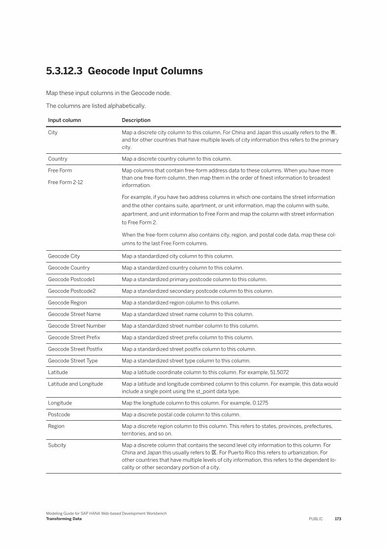
5.3.12.3 Geocode Input Columns
Map these input columns in the Geocode node.
The columns are listed alphabetically.
Input column Description
City Map a discrete city column to this column. For China and Japan this usually refers to the 市, and for other countries that have multiple levels of city information this refers to the primary city.
Country Map a discrete country column to this column.
Free Form
Free Form 2-12
Map columns that contain free-form address data to these columns. When you have more than one free-form column, then map them in the order of finest information to broadest information.
For example, if you have two address columns in which one contains the street information and the other contains suite, apartment, or unit information, map the column with suite, apartment, and unit information to Free Form and map the column with street information to Free Form 2.
When the free-form column also contains city, region, and postal code data, map these columns to the last Free Form columns.
Geocode City Map a standardized city column to this column.
Geocode Country Map a standardized country column to this column.
Geocode Postcode1 Map a standardized primary postcode column to this column.
Geocode Postcode2 Map a standardized secondary postcode column to this column.
Geocode Region Map a standardized region column to this column.
Geocode Street Name Map a standardized street name column to this column.
Geocode Street Number Map a standardized street number column to this column.
Geocode Street Prefix Map a standardized street prefix column to this column.
Geocode Street Postfix Map a standardized street postfix column to this column.
Geocode Street Type Map a standardized street type column to this column.
Latitude Map a latitude coordinate column to this column. For example, 51.5072
Latitude and Longitude Map a latitude and longitude combined column to this column. For example, this data would include a single point using the st_point data type.
Longitude Map the longitude column to this column. For example, 0.1275
Postcode Map a discrete postal code column to this column.
Region Map a discrete region column to this column. This refers to states, provinces, prefectures, territories, and so on.
Subcity Map a discrete column that contains the second level city information to this column. For China and Japan this usually refers to 区. For Puerto Rico this refers to urbanization. For other countries that have multiple levels of city information, this refers to the dependent locality or other secondary portion of a city.
Modeling Guide for SAP HANA Web-based Development WorkbenchTransforming Data PUBLIC 173
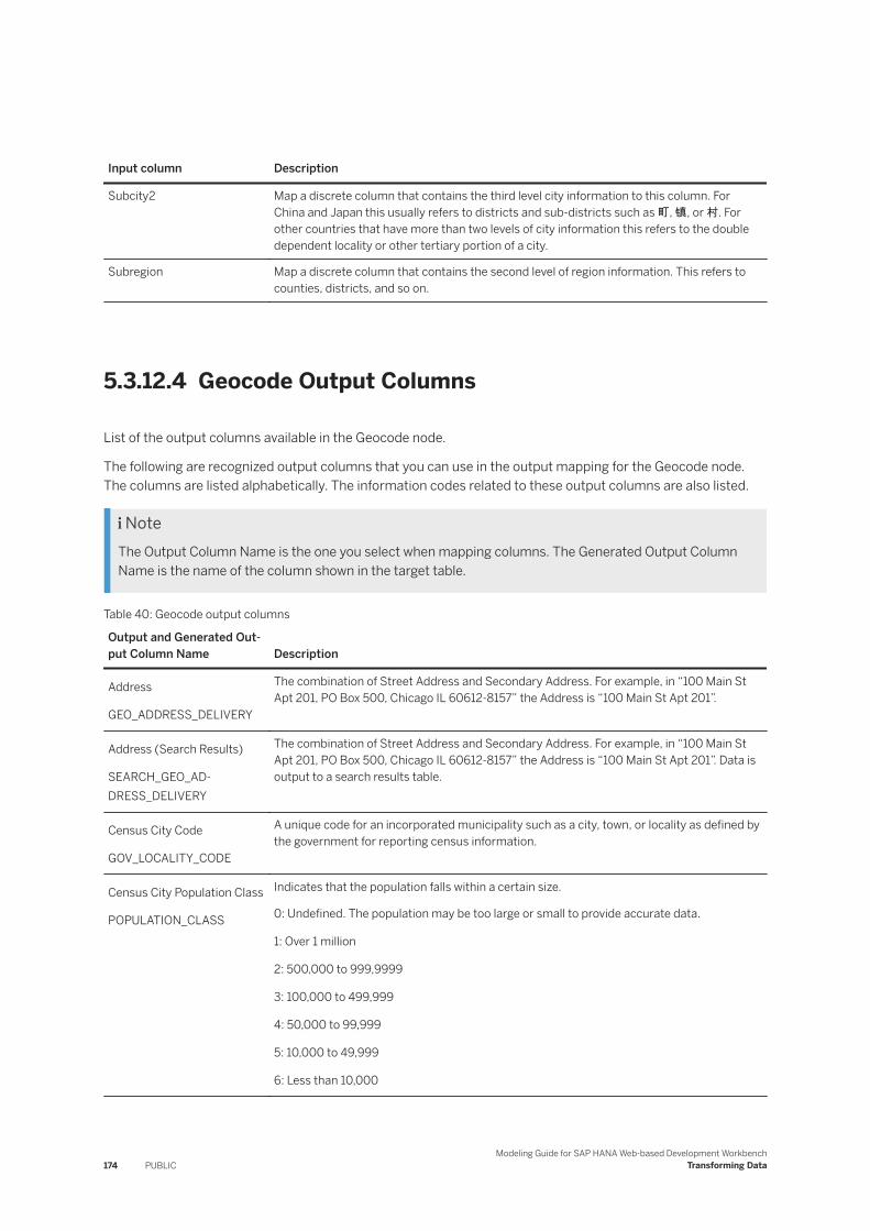
Input column Description
Subcity2 Map a discrete column that contains the third level city information to this column. For China and Japan this usually refers to districts and sub-districts such as 町, 镇, or 村. For other countries that have more than two levels of city information this refers to the double dependent locality or other tertiary portion of a city.
Subregion Map a discrete column that contains the second level of region information. This refers to counties, districts, and so on.
5.3.12.4 Geocode Output Columns
List of the output columns available in the Geocode node.
The following are recognized output columns that you can use in the output mapping for the Geocode node. The columns are listed alphabetically. The information codes related to these output columns are also listed.
NoteThe Output Column Name is the one you select when mapping columns. The Generated Output Column Name is the name of the column shown in the target table.
Table 40: Geocode output columns
Output and Generated Output Column Name Description
Address
GEO_ADDRESS_DELIVERY
The combination of Street Address and Secondary Address. For example, in “100 Main St Apt 201, PO Box 500, Chicago IL 60612-8157” the Address is “100 Main St Apt 201”.
Address (Search Results)
SEARCH_GEO_ADDRESS_DELIVERY
The combination of Street Address and Secondary Address. For example, in “100 Main St Apt 201, PO Box 500, Chicago IL 60612-8157” the Address is “100 Main St Apt 201”. Data is output to a search results table.
Census City Code
GOV_LOCALITY_CODE
A unique code for an incorporated municipality such as a city, town, or locality as defined by the government for reporting census information.
Census City Population Class
POPULATION_CLASS
Indicates that the population falls within a certain size.
0: Undefined. The population may be too large or small to provide accurate data.
1: Over 1 million
2: 500,000 to 999,9999
3: 100,000 to 499,999
4: 50,000 to 99,999
5: 10,000 to 49,999
6: Less than 10,000
174 PUBLICModeling Guide for SAP HANA Web-based Development Workbench
Transforming Data
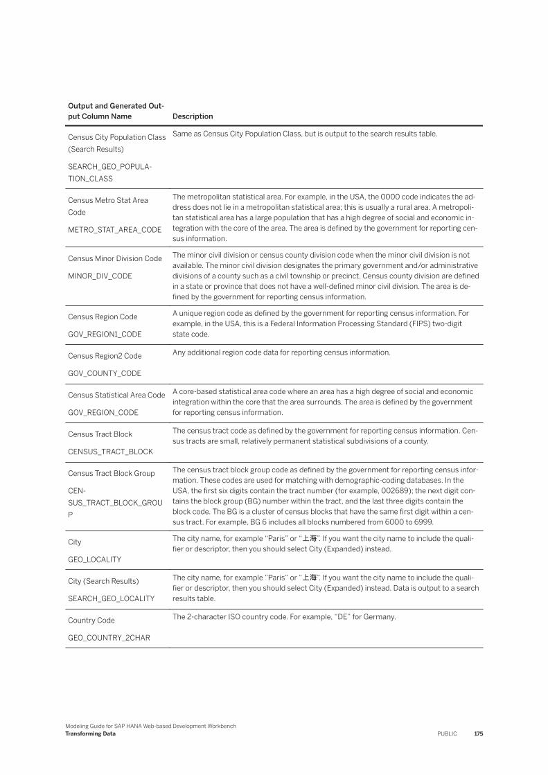
Output and Generated Output Column Name Description
Census City Population Class (Search Results)
SEARCH_GEO_POPULATION_CLASS
Same as Census City Population Class, but is output to the search results table.
Census Metro Stat Area Code
METRO_STAT_AREA_CODE
The metropolitan statistical area. For example, in the USA, the 0000 code indicates the address does not lie in a metropolitan statistical area; this is usually a rural area. A metropolitan statistical area has a large population that has a high degree of social and economic integration with the core of the area. The area is defined by the government for reporting census information.
Census Minor Division Code
MINOR_DIV_CODE
The minor civil division or census county division code when the minor civil division is not available. The minor civil division designates the primary government and/or administrative divisions of a county such as a civil township or precinct. Census county division are defined in a state or province that does not have a well-defined minor civil division. The area is defined by the government for reporting census information.
Census Region Code
GOV_REGION1_CODE
A unique region code as defined by the government for reporting census information. For example, in the USA, this is a Federal Information Processing Standard (FIPS) two-digit state code.
Census Region2 Code
GOV_COUNTY_CODE
Any additional region code data for reporting census information.
Census Statistical Area Code
GOV_REGION_CODE
A core-based statistical area code where an area has a high degree of social and economic integration within the core that the area surrounds. The area is defined by the government for reporting census information.
Census Tract Block
CENSUS_TRACT_BLOCK
The census tract code as defined by the government for reporting census information. Census tracts are small, relatively permanent statistical subdivisions of a county.
Census Tract Block Group
CENSUS_TRACT_BLOCK_GROUP
The census tract block group code as defined by the government for reporting census information. These codes are used for matching with demographic-coding databases. In the USA, the first six digits contain the tract number (for example, 002689); the next digit contains the block group (BG) number within the tract, and the last three digits contain the block code. The BG is a cluster of census blocks that have the same first digit within a census tract. For example, BG 6 includes all blocks numbered from 6000 to 6999.
City
GEO_LOCALITY
The city name, for example “Paris” or “上海”. If you want the city name to include the qualifier or descriptor, then you should select City (Expanded) instead.
City (Search Results)
SEARCH_GEO_LOCALITY
The city name, for example “Paris” or “上海”. If you want the city name to include the qualifier or descriptor, then you should select City (Expanded) instead. Data is output to a search results table.
Country Code
GEO_COUNTRY_2CHAR
The 2-character ISO country code. For example, “DE” for Germany.
Modeling Guide for SAP HANA Web-based Development WorkbenchTransforming Data PUBLIC 175
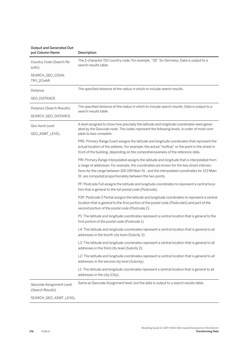
Output and Generated Output Column Name Description
Country Code (Search Results)
SEARCH_GEO_COUNTRY_2CHAR
The 2-character ISO country code. For example, “DE” for Germany. Data is output to a search results table.
Distance
GEO_DISTANCE
The specified distance of the radius in which to include search results.
Distance (Search Results)
SEARCH_GEO_DISTANCE
The specified distance of the radius in which to include search results. Data is output to a search results table.
Geo Asmt Level
GEO_ASMT_LEVEL
A level assigned to show how precisely the latitude and longitude coordinates were generated by the Geocode node. The codes represent the following levels, in order of most complete to less complete:
PRE: Primary Range Exact assigns the latitude and longitude coordinates that represent the actual location of the address. For example, the actual "rooftop" or the point in the street in front of the building, depending on the comprehensiveness of the reference data.
PRI: Primary Range Interpolated assigns the latitude and longitude that is interpolated from a range of addresses. For example, the coordinates are known for the two street intersections for the range between 100-199 Main St., and the interpolated coordinates for 123 Main St. are computed proportionately between the two points.
PF: Postcode Full assigns the latitude and longitude coordinates to represent a central location that is general to the full postal code (Postcode).
P2P: Postcode 2 Partial assigns the latitude and longitude coordinates to represent a central location that is general to the first portion of the postal code (Postcode1) and part of the second portion of the postal code (Postcode 2).
P1: The latitude and longitude coordinates represent a central location that is general to the first portion of the postal code (Postcode 1).
L4: The latitude and longitude coordinates represent a central location that is general to all addresses in the fourth city level (Subcity 3).
L3: The latitude and longitude coordinates represent a central location that is general to all addresses in the third city level (Subcity 2).
L2: The latitude and longitude coordinates represent a central location that is general to all addresses in the second city level (Subcity).
L1: The latitude and longitude coordinates represent a central location that is general to all addresses in the city (City).
Geocode Assignment Level (Search Results)
SEARCH_GEO_ASMT_LEVEL
Same as Geocode Assignment level, but the data is output to a search results table.
176 PUBLICModeling Guide for SAP HANA Web-based Development Workbench
Transforming Data
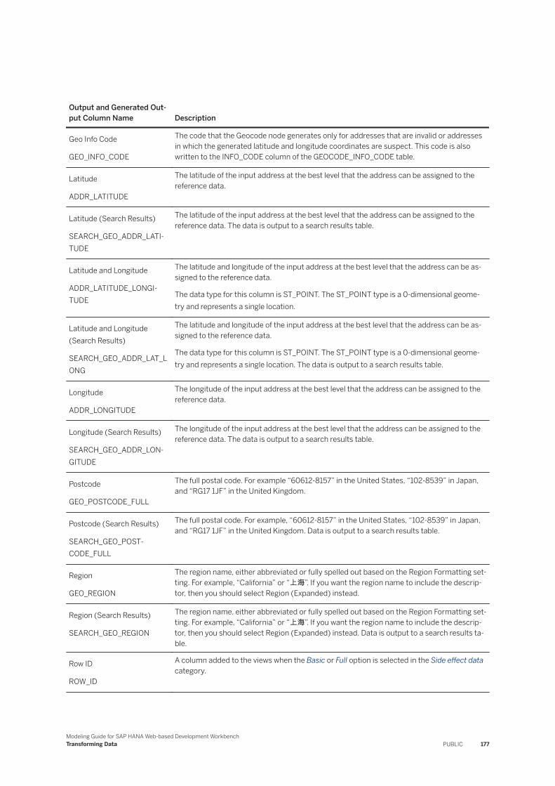
Output and Generated Output Column Name Description
Geo Info Code
GEO_INFO_CODE
The code that the Geocode node generates only for addresses that are invalid or addresses in which the generated latitude and longitude coordinates are suspect. This code is also written to the INFO_CODE column of the GEOCODE_INFO_CODE table.
Latitude
ADDR_LATITUDE
The latitude of the input address at the best level that the address can be assigned to the reference data.
Latitude (Search Results)
SEARCH_GEO_ADDR_LATITUDE
The latitude of the input address at the best level that the address can be assigned to the reference data. The data is output to a search results table.
Latitude and Longitude
ADDR_LATITUDE_LONGITUDE
The latitude and longitude of the input address at the best level that the address can be assigned to the reference data.
The data type for this column is ST_POINT. The ST_POINT type is a 0-dimensional geometry and represents a single location.
Latitude and Longitude (Search Results)
SEARCH_GEO_ADDR_LAT_LONG
The latitude and longitude of the input address at the best level that the address can be assigned to the reference data.
The data type for this column is ST_POINT. The ST_POINT type is a 0-dimensional geometry and represents a single location. The data is output to a search results table.
Longitude
ADDR_LONGITUDE
The longitude of the input address at the best level that the address can be assigned to the reference data.
Longitude (Search Results)
SEARCH_GEO_ADDR_LONGITUDE
The longitude of the input address at the best level that the address can be assigned to the reference data. The data is output to a search results table.
Postcode
GEO_POSTCODE_FULL
The full postal code. For example “60612-8157” in the United States, “102-8539” in Japan, and “RG17 1JF” in the United Kingdom.
Postcode (Search Results)
SEARCH_GEO_POSTCODE_FULL
The full postal code. For example, “60612-8157” in the United States, “102-8539” in Japan, and “RG17 1JF” in the United Kingdom. Data is output to a search results table.
Region
GEO_REGION
The region name, either abbreviated or fully spelled out based on the Region Formatting setting. For example, “California” or “上海”. If you want the region name to include the descriptor, then you should select Region (Expanded) instead.
Region (Search Results)
SEARCH_GEO_REGION
The region name, either abbreviated or fully spelled out based on the Region Formatting setting. For example, “California” or “上海”. If you want the region name to include the descriptor, then you should select Region (Expanded) instead. Data is output to a search results table.
Row ID
ROW_ID
A column added to the views when the Basic or Full option is selected in the Side effect data category.
Modeling Guide for SAP HANA Web-based Development WorkbenchTransforming Data PUBLIC 177
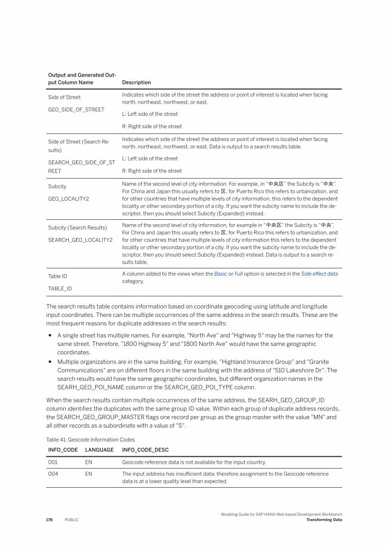
Output and Generated Output Column Name Description
Side of Street
GEO_SIDE_OF_STREET
Indicates which side of the street the address or point of interest is located when facing north, northeast, northwest, or east.
L: Left side of the street
R: Right side of the street
Side of Street (Search Results)
SEARCH_GEO_SIDE_OF_STREET
Indicates which side of the street the address or point of interest is located when facing north, northeast, northwest, or east. Data is output to a search results table.
L: Left side of the street
R: Right side of the street
Subcity
GEO_LOCALITY2
Name of the second level of city information. For example, in “中央区” the Subcity is “中央”. For China and Japan this usually refers to 区, for Puerto Rico this refers to urbanization, and for other countries that have multiple levels of city information, this refers to the dependent locality or other secondary portion of a city. If you want the subcity name to include the descriptor, then you should select Subcity (Expanded) instead.
Subcity (Search Results)
SEARCH_GEO_LOCALITY2
Name of the second level of city information, for example in “中央区” the Subcity is “中央”. For China and Japan this usually refers to 区, for Puerto Rico this refers to urbanization, and for other countries that have multiple levels of city information this refers to the dependent locality or other secondary portion of a city. If you want the subcity name to include the descriptor, then you should select Subcity (Expanded) instead. Data is output to a search results table.
Table ID
TABLE_ID
A column added to the views when the Basic or Full option is selected in the Side effect data category.
The search results table contains information based on coordinate geocoding using latitude and longitude input coordinates. There can be multiple occurrences of the same address in the search results. These are the most frequent reasons for duplicate addresses in the search results:
● A single street has multiple names. For example, "North Ave" and "Highway 5" may be the names for the same street. Therefore, "1800 Highway 5" and "1800 North Ave" would have the same geographic coordinates.
● Multiple organizations are in the same building. For example, "Highland Insurance Group" and "Granite Communications" are on different floors in the same building with the address of "510 Lakeshore Dr". The search results would have the same geographic coordinates, but different organization names in the SEARH_GEO_POI_NAME column or the SEARCH_GEO_POI_TYPE column.
When the search results contain multiple occurrences of the same address, the SEARH_GEO_GROUP_ID column identifies the duplicates with the same group ID value. Within each group of duplicate address records, the SEARCH_GEO_GROUP_MASTER flags one record per group as the group master with the value "MN" and all other records as a subordinate with a value of "S".
Table 41: Geocode Information Codes
INFO_CODE LANGUAGE INFO_CODE_DESC
001 EN Geocode reference data is not available for the input country.
004 EN The input address has insufficient data; therefore assignment to the Geocode reference data is at a lower quality level than expected.
178 PUBLICModeling Guide for SAP HANA Web-based Development Workbench
Transforming Data
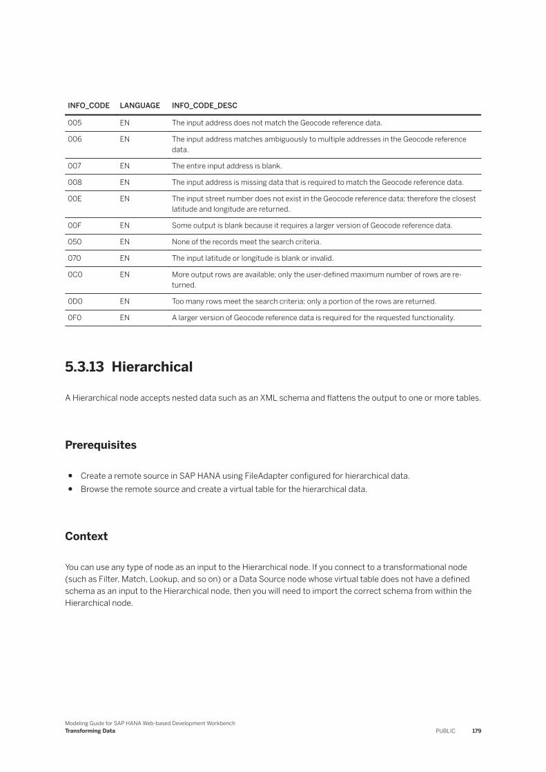
INFO_CODE LANGUAGE INFO_CODE_DESC
005 EN The input address does not match the Geocode reference data.
006 EN The input address matches ambiguously to multiple addresses in the Geocode reference data.
007 EN The entire input address is blank.
008 EN The input address is missing data that is required to match the Geocode reference data.
00E EN The input street number does not exist in the Geocode reference data; therefore the closest latitude and longitude are returned.
00F EN Some output is blank because it requires a larger version of Geocode reference data.
050 EN None of the records meet the search criteria.
070 EN The input latitude or longitude is blank or invalid.
0C0 EN More output rows are available; only the user-defined maximum number of rows are returned.
0D0 EN Too many rows meet the search criteria; only a portion of the rows are returned.
0F0 EN A larger version of Geocode reference data is required for the requested functionality.
5.3.13 Hierarchical
A Hierarchical node accepts nested data such as an XML schema and flattens the output to one or more tables.
Prerequisites
● Create a remote source in SAP HANA using FileAdapter configured for hierarchical data.● Browse the remote source and create a virtual table for the hierarchical data.
Context
You can use any type of node as an input to the Hierarchical node. If you connect to a transformational node (such as Filter, Match, Lookup, and so on) or a Data Source node whose virtual table does not have a defined schema as an input to the Hierarchical node, then you will need to import the correct schema from within the Hierarchical node.
Modeling Guide for SAP HANA Web-based Development WorkbenchTransforming Data PUBLIC 179
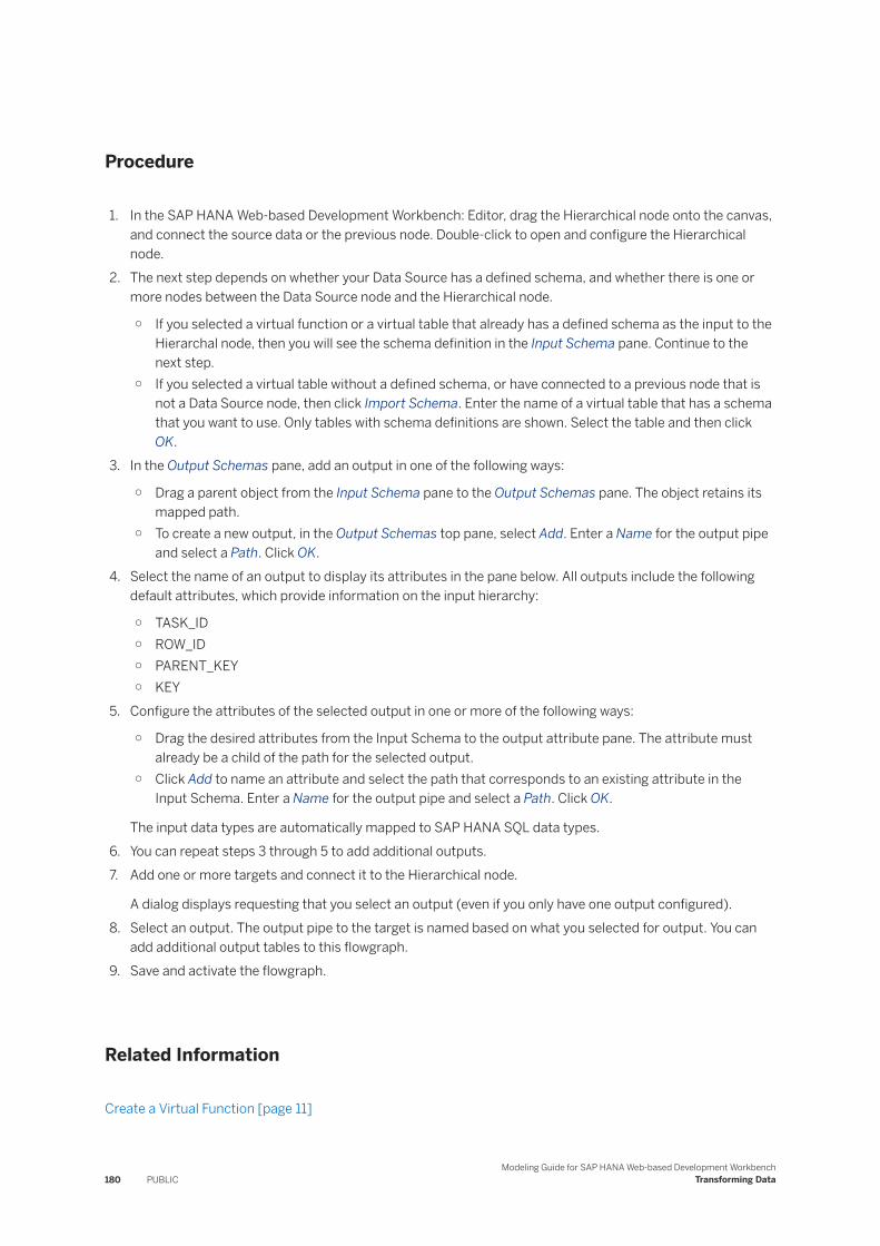
Procedure
1. In the SAP HANA Web-based Development Workbench: Editor, drag the Hierarchical node onto the canvas, and connect the source data or the previous node. Double-click to open and configure the Hierarchical node.
2. The next step depends on whether your Data Source has a defined schema, and whether there is one or more nodes between the Data Source node and the Hierarchical node.
○ If you selected a virtual function or a virtual table that already has a defined schema as the input to the Hierarchal node, then you will see the schema definition in the Input Schema pane. Continue to the next step.
○ If you selected a virtual table without a defined schema, or have connected to a previous node that is not a Data Source node, then click Import Schema. Enter the name of a virtual table that has a schema that you want to use. Only tables with schema definitions are shown. Select the table and then click OK.
3. In the Output Schemas pane, add an output in one of the following ways:
○ Drag a parent object from the Input Schema pane to the Output Schemas pane. The object retains its mapped path.
○ To create a new output, in the Output Schemas top pane, select Add. Enter a Name for the output pipe and select a Path. Click OK.
4. Select the name of an output to display its attributes in the pane below. All outputs include the following default attributes, which provide information on the input hierarchy:
○ TASK_ID○ ROW_ID○ PARENT_KEY○ KEY
5. Configure the attributes of the selected output in one or more of the following ways:
○ Drag the desired attributes from the Input Schema to the output attribute pane. The attribute must already be a child of the path for the selected output.
○ Click Add to name an attribute and select the path that corresponds to an existing attribute in the Input Schema. Enter a Name for the output pipe and select a Path. Click OK.
The input data types are automatically mapped to SAP HANA SQL data types.6. You can repeat steps 3 through 5 to add additional outputs.7. Add one or more targets and connect it to the Hierarchical node.
A dialog displays requesting that you select an output (even if you only have one output configured).8. Select an output. The output pipe to the target is named based on what you selected for output. You can
add additional output tables to this flowgraph.9. Save and activate the flowgraph.
Related Information
Create a Virtual Function [page 11]
180 PUBLICModeling Guide for SAP HANA Web-based Development Workbench
Transforming Data
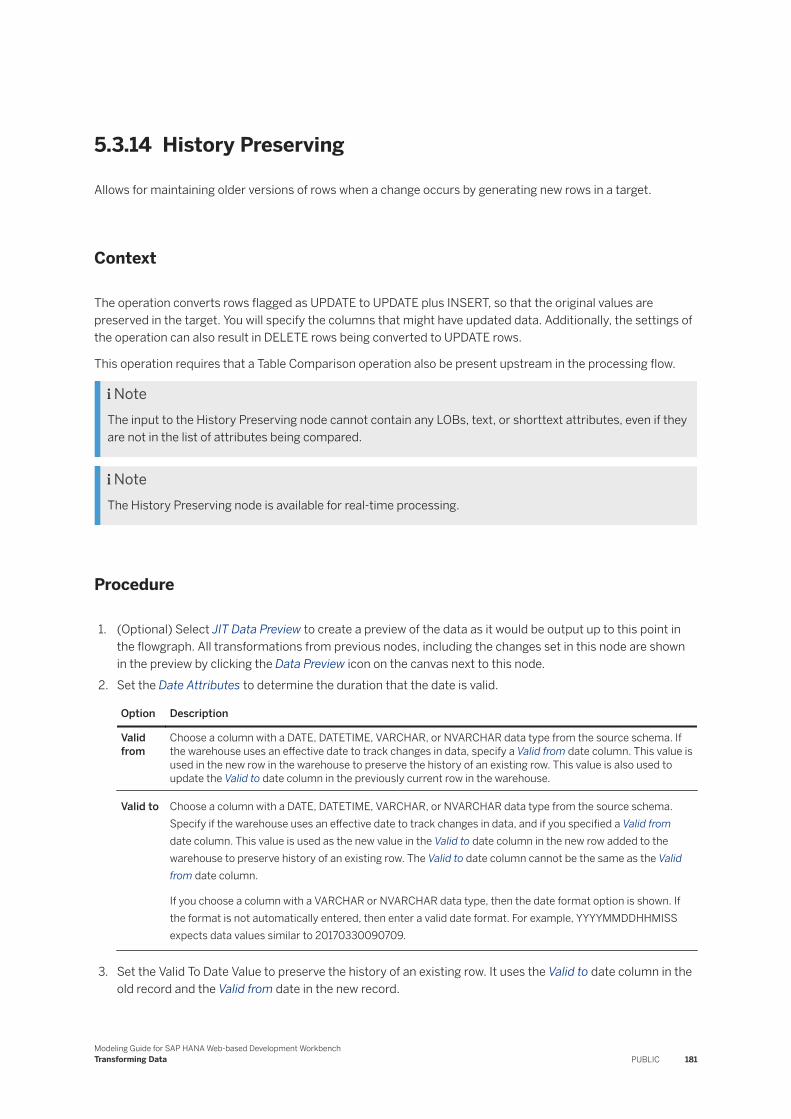
5.3.14 History Preserving
Allows for maintaining older versions of rows when a change occurs by generating new rows in a target.
Context
The operation converts rows flagged as UPDATE to UPDATE plus INSERT, so that the original values are preserved in the target. You will specify the columns that might have updated data. Additionally, the settings of the operation can also result in DELETE rows being converted to UPDATE rows.
This operation requires that a Table Comparison operation also be present upstream in the processing flow.
NoteThe input to the History Preserving node cannot contain any LOBs, text, or shorttext attributes, even if they are not in the list of attributes being compared.
NoteThe History Preserving node is available for real-time processing.
Procedure
1. (Optional) Select JIT Data Preview to create a preview of the data as it would be output up to this point in the flowgraph. All transformations from previous nodes, including the changes set in this node are shown in the preview by clicking the Data Preview icon on the canvas next to this node.
2. Set the Date Attributes to determine the duration that the date is valid.
Option Description
Valid from
Choose a column with a DATE, DATETIME, VARCHAR, or NVARCHAR data type from the source schema. If the warehouse uses an effective date to track changes in data, specify a Valid from date column. This value is used in the new row in the warehouse to preserve the history of an existing row. This value is also used to update the Valid to date column in the previously current row in the warehouse.
Valid to Choose a column with a DATE, DATETIME, VARCHAR, or NVARCHAR data type from the source schema. Specify if the warehouse uses an effective date to track changes in data, and if you specified a Valid from date column. This value is used as the new value in the Valid to date column in the new row added to the warehouse to preserve history of an existing row. The Valid to date column cannot be the same as the Valid from date column.
If you choose a column with a VARCHAR or NVARCHAR data type, then the date format option is shown. If the format is not automatically entered, then enter a valid date format. For example, YYYYMMDDHHMISS expects data values similar to 20170330090709.
3. Set the Valid To Date Value to preserve the history of an existing row. It uses the Valid to date column in the old record and the Valid from date in the new record.
Modeling Guide for SAP HANA Web-based Development WorkbenchTransforming Data PUBLIC 181

Option Description
New record
Specify a date value
Old record
○ Use "Valid From" date of the new record: The following example shows that the new record (Key 2) column From_Date contains the date 2016.03.20 and the old record (Key 1) To_Date column contains the same value.
Key Empl_ID Name Salary From_Date To_Date
1 567 Kramer 1000 2015.03.25 2016.03.20
2 567 Kramer 1200 2016.03.20 9000.12.31
○ Use one day before "Valid From" date of new record: The following example shows that the new record (Key 2) From_Date column contains 2016.03.19 and the old record (Key 1) To_Date column contains a date that is one day before that value, 2016.03.20.
Key Empl_ID Name Salary From_Date To_Date
1 567 Kramer 1000 2015.03.25 2016.03.20
2 567 Kramer 1200 2016.03.19 9000.12.31
NoteIf you choose a column with a VARCHAR or NVARCHAR data type and select Use one day before "Valid From" date of new record, enter the date format in the Valid from Attribute.
4. Click the + icon to select the column or columns that you want to compare. The column or columns in the input data set for which this transform compares the before- and after-images to determine whether there are changes.○ If the values in each image of the data match, the row is flagged to Update. The result updates the
warehouse row with values from the new row. The row from the before-image is included in the output as Update to effectively update the date and flag information.
○ If the values in each image do not match, the row from the after-image is flagged as Insert, and included in the output. The result adds a new row to the warehouse with the values from the new row.
5. Under Current Flag, select the Attribute value to select the source column that identifies the current valid row from a set of rows with the same primary key. This indicates whether a row is the most current data in the warehouse for a given primary key.
6. Enter the Set value. This value evaluates the column data in the Attribute option. This value is used to update the current flag Attribute in the new row in the warehouse added to preserve the history of an existing row.
7. Enter the Reset value. This value evaluates the column data in the Attribute option. This value is used to update the current flag Attribute in the existing row in warehouse that included changes in one or more of the compare columns.
8. (Optional) Select whether you want to Update attribute on deletion. Selecting this option converts Delete rows to Update rows in the target. If you set the Date Attributes options (Valid from and Valid to), the Valid to option becomes the processing date. Use this option to maintain slowly changing dimensions by feeding a complete data set first through the Table Comparison node with its Detect deleted row(s) from
182 PUBLICModeling Guide for SAP HANA Web-based Development Workbench
Transforming Data
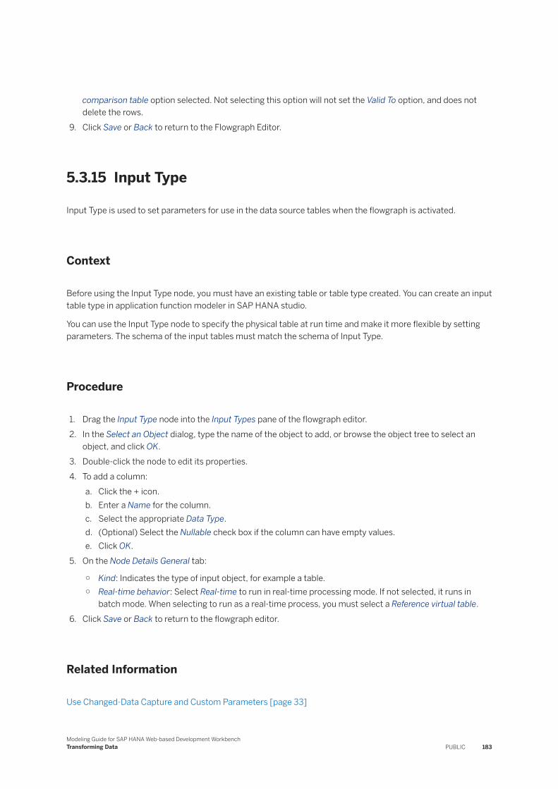
comparison table option selected. Not selecting this option will not set the Valid To option, and does not delete the rows.
9. Click Save or Back to return to the Flowgraph Editor.
5.3.15 Input Type
Input Type is used to set parameters for use in the data source tables when the flowgraph is activated.
Context
Before using the Input Type node, you must have an existing table or table type created. You can create an input table type in application function modeler in SAP HANA studio.
You can use the Input Type node to specify the physical table at run time and make it more flexible by setting parameters. The schema of the input tables must match the schema of Input Type.
Procedure
1. Drag the Input Type node into the Input Types pane of the flowgraph editor.2. In the Select an Object dialog, type the name of the object to add, or browse the object tree to select an
object, and click OK.3. Double-click the node to edit its properties.4. To add a column:
a. Click the + icon.b. Enter a Name for the column.c. Select the appropriate Data Type.d. (Optional) Select the Nullable check box if the column can have empty values.e. Click OK.
5. On the Node Details General tab:
○ Kind: Indicates the type of input object, for example a table.○ Real-time behavior: Select Real-time to run in real-time processing mode. If not selected, it runs in
batch mode. When selecting to run as a real-time process, you must select a Reference virtual table.6. Click Save or Back to return to the flowgraph editor.
Related Information
Use Changed-Data Capture and Custom Parameters [page 33]
Modeling Guide for SAP HANA Web-based Development WorkbenchTransforming Data PUBLIC 183
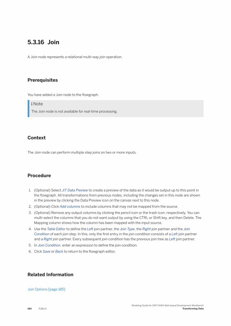
5.3.16 Join
A Join node represents a relational multi-way join operation.
Prerequisites
You have added a Join node to the flowgraph.
NoteThe Join node is not available for real-time processing.
Context
The Join node can perform multiple step joins on two or more inputs.
Procedure
1. (Optional) Select JIT Data Preview to create a preview of the data as it would be output up to this point in the flowgraph. All transformations from previous nodes, including the changes set in this node are shown in the preview by clicking the Data Preview icon on the canvas next to this node.
2. (Optional) Click Add columns to include columns that may not be mapped from the source.3. (Optional) Remove any output columns by clicking the pencil icon or the trash icon, respectively. You can
multi-select the columns that you do not want output by using the CTRL or Shift key, and then Delete. The Mapping column shows how the column has been mapped with the input source.
4. Use the Table Editor to define the Left join partner, the Join Type, the Right join partner and the Join Condition of each join step. In this, only the first entry in the join condition consists of a Left join partner and a Right join partner. Every subsequent join condition has the previous join tree as Left join partner.
5. In Join Condition, enter an expression to define the join condition.6. Click Save or Back to return to the flowgraph editor.
Related Information
Join Options [page 185]
184 PUBLICModeling Guide for SAP HANA Web-based Development Workbench
Transforming Data
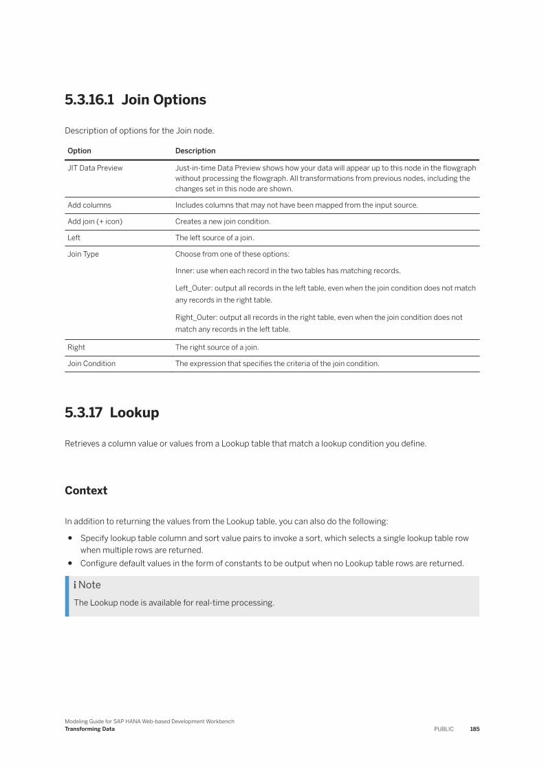
5.3.16.1 Join Options
Description of options for the Join node.
Option Description
JIT Data Preview Just-in-time Data Preview shows how your data will appear up to this node in the flowgraph without processing the flowgraph. All transformations from previous nodes, including the changes set in this node are shown.
Add columns Includes columns that may not have been mapped from the input source.
Add join (+ icon) Creates a new join condition.
Left The left source of a join.
Join Type Choose from one of these options:
Inner: use when each record in the two tables has matching records.
Left_Outer: output all records in the left table, even when the join condition does not match any records in the right table.
Right_Outer: output all records in the right table, even when the join condition does not match any records in the left table.
Right The right source of a join.
Join Condition The expression that specifies the criteria of the join condition.
5.3.17 Lookup
Retrieves a column value or values from a Lookup table that match a lookup condition you define.
Context
In addition to returning the values from the Lookup table, you can also do the following:
● Specify lookup table column and sort value pairs to invoke a sort, which selects a single lookup table row when multiple rows are returned.
● Configure default values in the form of constants to be output when no Lookup table rows are returned.
NoteThe Lookup node is available for real-time processing.
Modeling Guide for SAP HANA Web-based Development WorkbenchTransforming Data PUBLIC 185
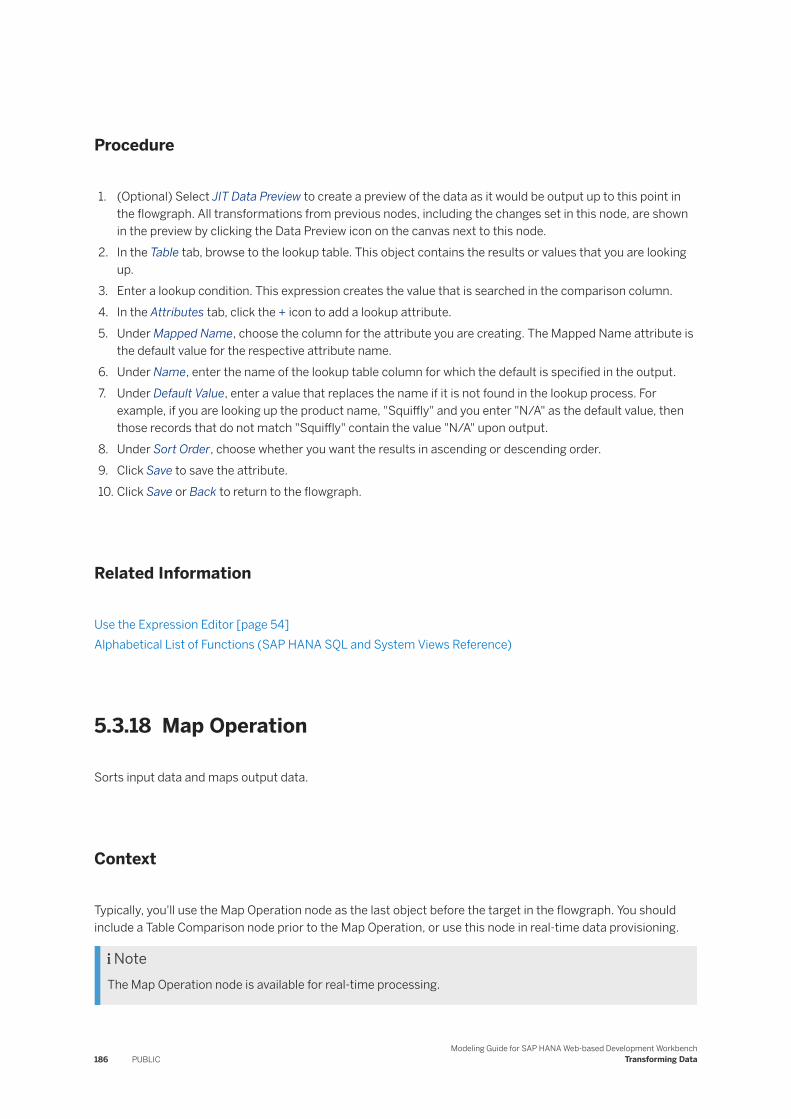
Procedure
1. (Optional) Select JIT Data Preview to create a preview of the data as it would be output up to this point in the flowgraph. All transformations from previous nodes, including the changes set in this node, are shown in the preview by clicking the Data Preview icon on the canvas next to this node.
2. In the Table tab, browse to the lookup table. This object contains the results or values that you are looking up.
3. Enter a lookup condition. This expression creates the value that is searched in the comparison column.4. In the Attributes tab, click the + icon to add a lookup attribute.5. Under Mapped Name, choose the column for the attribute you are creating. The Mapped Name attribute is
the default value for the respective attribute name.6. Under Name, enter the name of the lookup table column for which the default is specified in the output.7. Under Default Value, enter a value that replaces the name if it is not found in the lookup process. For
example, if you are looking up the product name, "Squiffly" and you enter "N/A" as the default value, then those records that do not match "Squiffly" contain the value "N/A" upon output.
8. Under Sort Order, choose whether you want the results in ascending or descending order.9. Click Save to save the attribute.10. Click Save or Back to return to the flowgraph.
Related Information
Use the Expression Editor [page 54]Alphabetical List of Functions (SAP HANA SQL and System Views Reference)
5.3.18 Map Operation
Sorts input data and maps output data.
Context
Typically, you'll use the Map Operation node as the last object before the target in the flowgraph. You should include a Table Comparison node prior to the Map Operation, or use this node in real-time data provisioning.
NoteThe Map Operation node is available for real-time processing.
186 PUBLICModeling Guide for SAP HANA Web-based Development Workbench
Transforming Data
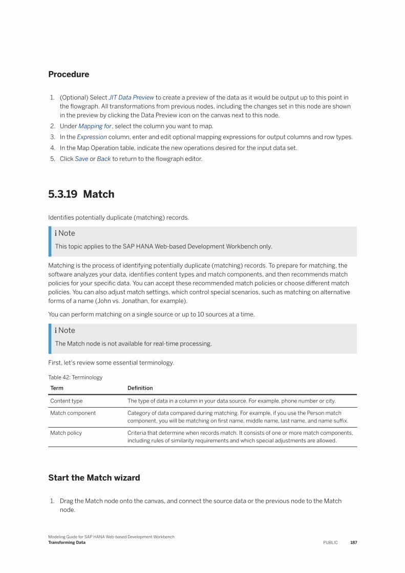
Procedure
1. (Optional) Select JIT Data Preview to create a preview of the data as it would be output up to this point in the flowgraph. All transformations from previous nodes, including the changes set in this node are shown in the preview by clicking the Data Preview icon on the canvas next to this node.
2. Under Mapping for, select the column you want to map.3. In the Expression column, enter and edit optional mapping expressions for output columns and row types.4. In the Map Operation table, indicate the new operations desired for the input data set.5. Click Save or Back to return to the flowgraph editor.
5.3.19 Match
Identifies potentially duplicate (matching) records.
NoteThis topic applies to the SAP HANA Web-based Development Workbench only.
Matching is the process of identifying potentially duplicate (matching) records. To prepare for matching, the software analyzes your data, identifies content types and match components, and then recommends match policies for your specific data. You can accept these recommended match policies or choose different match policies. You can also adjust match settings, which control special scenarios, such as matching on alternative forms of a name (John vs. Jonathan, for example).
You can perform matching on a single source or up to 10 sources at a time.
NoteThe Match node is not available for real-time processing.
First, let's review some essential terminology.
Table 42: Terminology
Term Definition
Content type The type of data in a column in your data source. For example, phone number or city.
Match component Category of data compared during matching. For example, if you use the Person match component, you will be matching on first name, middle name, last name, and name suffix.
Match policy Criteria that determine when records match. It consists of one or more match components, including rules of similarity requirements and which special adjustments are allowed.
Start the Match wizard
1. Drag the Match node onto the canvas, and connect the source data or the previous node to the Match node.
Modeling Guide for SAP HANA Web-based Development WorkbenchTransforming Data PUBLIC 187
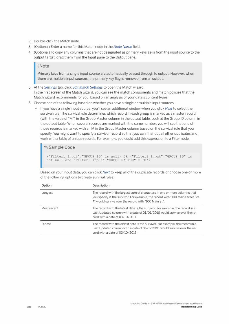
2. Double-click the Match node.3. (Optional) Enter a name for this Match node in the Node Name field.4. (Optional) To copy any columns that are not designated as primary keys as-is from the input source to the
output target, drag them from the Input pane to the Output pane.
NotePrimary keys from a single input source are automatically passed through to output. However, when there are multiple input sources, the primary key flag is removed from all output.
5. At the Settings tab, click Edit Match Settings to open the Match wizard.In the first screen of the Match wizard, you can see the match components and match policies that the Match wizard recommends for you, based on an analysis of your data's content types.
6. Choose one of the following based on whether you have a single or multiple input sources.○ If you have a single input source, you'll see an additional window when you click Next to select the
survival rule. The survival rule determines which record in each group is marked as a master record (with the value of "M") in the Group Master column in the output table. Look at the Group ID column in the output table. When several records are marked with the same number, you will see that one of those records is marked with an M in the Group Master column based on the survival rule that you specify. You might want to specify a survivor record so that you can filter out all other duplicates and work with a table of unique records. For example, you could add this expression to a Filter node:
Sample Code
("Filter1_Input"."GROUP_ID" is null) OR ("Filter1_Input"."GROUP_ID" is not null and "Filter1_Input"."GROUP_MASTER" = 'M')
Based on your input data, you can click Next to keep all of the duplicate records or choose one or more of the following options to create survival rules:
Option Description
Longest The record with the largest sum of characters in one or more columns that you specify is the survivor. For example, the record with "100 Main Street Ste A" would survive over the record with "100 Main St".
Most recent The record with the latest date is the survivor. For example, the record in a Last Updated column with a date of 01/01/2016 would survive over the record with a date of 03/10/2011.
Oldest The record with the oldest date is the survivor. For example, the record in a Last Updated column with a date of 06/12/2011 would survive over the record with a date of 03/10/2016.
188 PUBLICModeling Guide for SAP HANA Web-based Development Workbench
Transforming Data
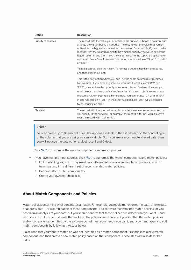
Option Description
Priority of sources The record with the value you prioritize is the survivor. Choose a column, and arrange the values based on priority. The record with the value that you prioritized as the highest is marked as the survivor. For example, if you consider records from the western region to be a higher priority, you would select the Region column, and then move the value "West" to the top. Any duplicate records with "West" would survive over records with a value of "South", "North" or "East".
To add a source, click the + icon. To remove a source, highlight the source, and then click the X icon.
This is the only option where you can use the same column multiple times. For example, if you have a System column with the values of "CRM" and "ERP", you can have two priority of sources rules on System. However, you must delete the other used values from the list in each rule. You cannot use the same value in both rules. For example, you cannot use "CRM" and "ERP" in one rule and only "ERP" in the other rule because "ERP" would be used twice, causing an error.
Shortest The record with the shortest sum of characters in one or more columns that you specify is the survivor. For example, the record with "CA" would survive over the record with "California".
NoteYou can create up to 10 survival rules. The options available in the list is based on the content type of the column that you are using as a survival rule. So, if you are using character-based data, then you will not see the date options, Most recent and Oldest.
Click Next to customize the match components and match policies.
○ If you have multiple input sources, click Next to customize the match components and match policies:○ Edit content types, which may result in a different list of available match components, which in
turn may result in a different set of recommended match policies.○ Define custom match components.○ Create your own match policies.
About Match Components and Policies
Match policies determine what constitutes a match. For example, you could match on name data, or firm data, or address data -- or a combination of these components. The software recommends match policies for you, based on an analysis of your data, but you should confirm that these polices are indeed what you want -- and also confirm that the components that make up the policies are accurate. If you find that the match policies and/or components identified by the software do not meet your needs, you can identify content types and edit match components by following the steps below.
If a column that you want to match on was not identified as a match component, first add it as a new match component, and then create a new match policy based on that component. These steps are also described below.
Modeling Guide for SAP HANA Web-based Development WorkbenchTransforming Data PUBLIC 189
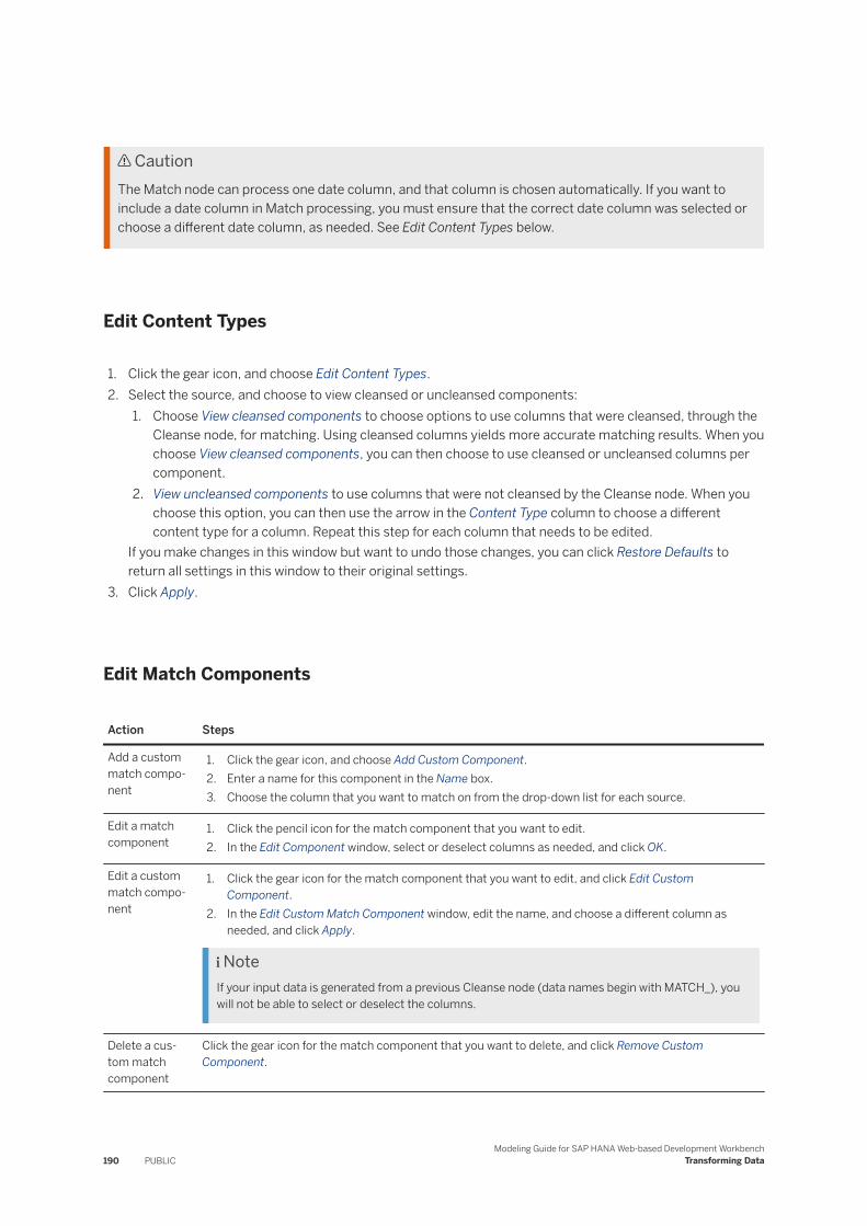
CautionThe Match node can process one date column, and that column is chosen automatically. If you want to include a date column in Match processing, you must ensure that the correct date column was selected or choose a different date column, as needed. See Edit Content Types below.
Edit Content Types
1. Click the gear icon, and choose Edit Content Types.2. Select the source, and choose to view cleansed or uncleansed components:
1. Choose View cleansed components to choose options to use columns that were cleansed, through the Cleanse node, for matching. Using cleansed columns yields more accurate matching results. When you choose View cleansed components, you can then choose to use cleansed or uncleansed columns per component.
2. View uncleansed components to use columns that were not cleansed by the Cleanse node. When you choose this option, you can then use the arrow in the Content Type column to choose a different content type for a column. Repeat this step for each column that needs to be edited.
If you make changes in this window but want to undo those changes, you can click Restore Defaults to return all settings in this window to their original settings.
3. Click Apply.
Edit Match Components
Action Steps
Add a custom match component
1. Click the gear icon, and choose Add Custom Component.2. Enter a name for this component in the Name box.3. Choose the column that you want to match on from the drop-down list for each source.
Edit a match component
1. Click the pencil icon for the match component that you want to edit.2. In the Edit Component window, select or deselect columns as needed, and click OK.
Edit a custom match component
1. Click the gear icon for the match component that you want to edit, and click Edit Custom Component.
2. In the Edit Custom Match Component window, edit the name, and choose a different column as needed, and click Apply.
NoteIf your input data is generated from a previous Cleanse node (data names begin with MATCH_), you will not be able to select or deselect the columns.
Delete a custom match component
Click the gear icon for the match component that you want to delete, and click Remove Custom Component.
190 PUBLICModeling Guide for SAP HANA Web-based Development Workbench
Transforming Data
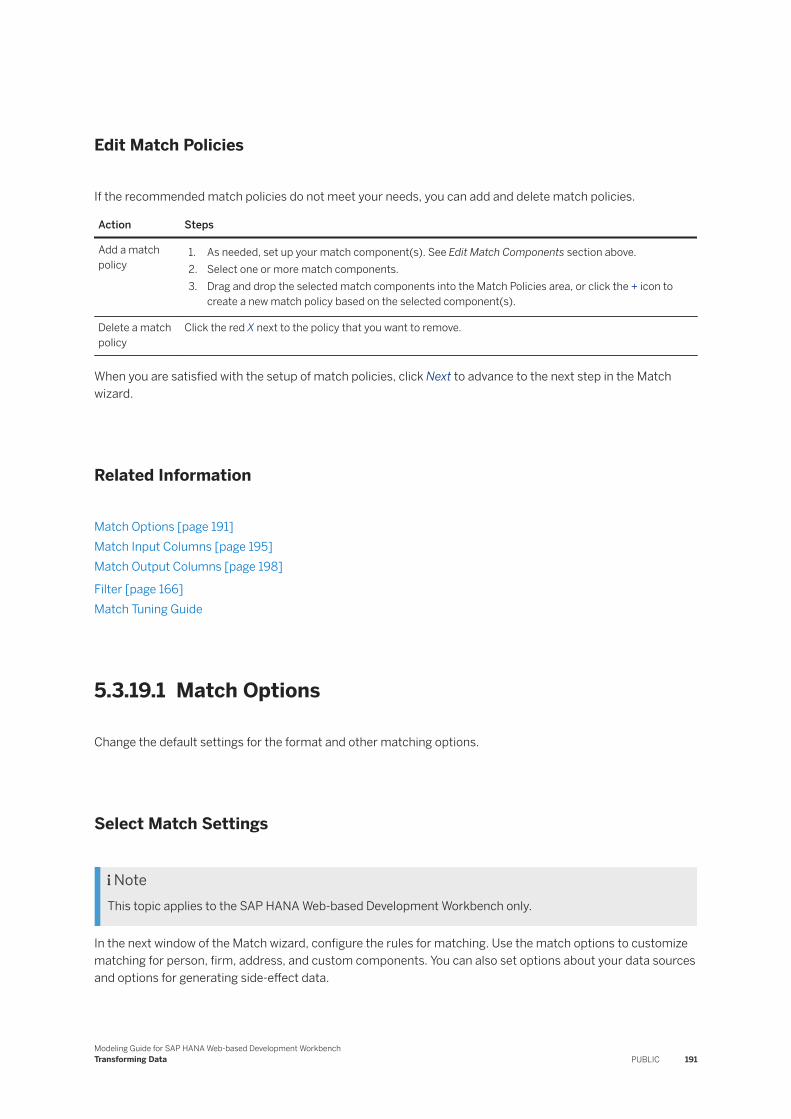
Edit Match Policies
If the recommended match policies do not meet your needs, you can add and delete match policies.
Action Steps
Add a match policy
1. As needed, set up your match component(s). See Edit Match Components section above.2. Select one or more match components.3. Drag and drop the selected match components into the Match Policies area, or click the + icon to
create a new match policy based on the selected component(s).
Delete a match policy
Click the red X next to the policy that you want to remove.
When you are satisfied with the setup of match policies, click Next to advance to the next step in the Match wizard.
Related Information
Match Options [page 191]Match Input Columns [page 195]Match Output Columns [page 198]
Filter [page 166]Match Tuning Guide
5.3.19.1 Match Options
Change the default settings for the format and other matching options.
Select Match Settings
NoteThis topic applies to the SAP HANA Web-based Development Workbench only.
In the next window of the Match wizard, configure the rules for matching. Use the match options to customize matching for person, firm, address, and custom components. You can also set options about your data sources and options for generating side-effect data.
Modeling Guide for SAP HANA Web-based Development WorkbenchTransforming Data PUBLIC 191
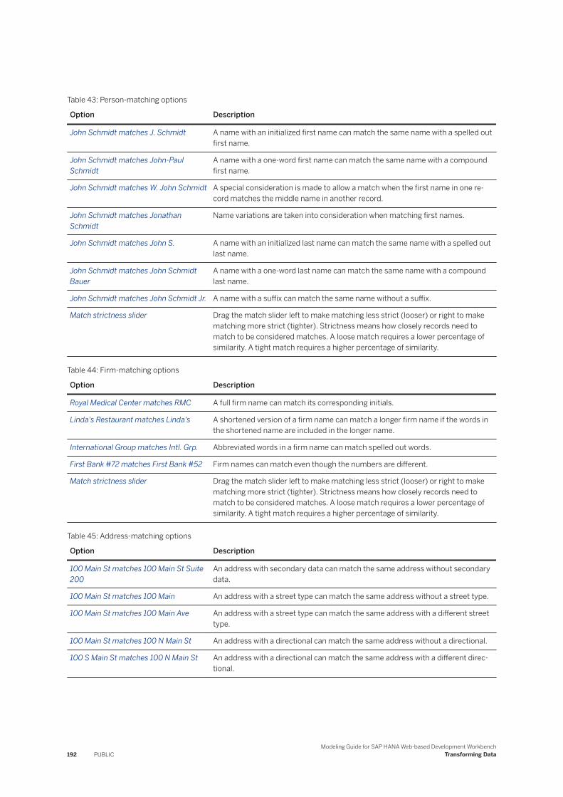
Table 43: Person-matching options
Option Description
John Schmidt matches J. Schmidt A name with an initialized first name can match the same name with a spelled out first name.
John Schmidt matches John-Paul Schmidt
A name with a one-word first name can match the same name with a compound first name.
John Schmidt matches W. John Schmidt A special consideration is made to allow a match when the first name in one record matches the middle name in another record.
John Schmidt matches Jonathan Schmidt
Name variations are taken into consideration when matching first names.
John Schmidt matches John S. A name with an initialized last name can match the same name with a spelled out last name.
John Schmidt matches John Schmidt Bauer
A name with a one-word last name can match the same name with a compound last name.
John Schmidt matches John Schmidt Jr. A name with a suffix can match the same name without a suffix.
Match strictness slider Drag the match slider left to make matching less strict (looser) or right to make matching more strict (tighter). Strictness means how closely records need to match to be considered matches. A loose match requires a lower percentage of similarity. A tight match requires a higher percentage of similarity.
Table 44: Firm-matching options
Option Description
Royal Medical Center matches RMC A full firm name can match its corresponding initials.
Linda's Restaurant matches Linda's A shortened version of a firm name can match a longer firm name if the words in the shortened name are included in the longer name.
International Group matches Intl. Grp. Abbreviated words in a firm name can match spelled out words.
First Bank #72 matches First Bank #52 Firm names can match even though the numbers are different.
Match strictness slider Drag the match slider left to make matching less strict (looser) or right to make matching more strict (tighter). Strictness means how closely records need to match to be considered matches. A loose match requires a lower percentage of similarity. A tight match requires a higher percentage of similarity.
Table 45: Address-matching options
Option Description
100 Main St matches 100 Main St Suite 200
An address with secondary data can match the same address without secondary data.
100 Main St matches 100 Main An address with a street type can match the same address without a street type.
100 Main St matches 100 Main Ave An address with a street type can match the same address with a different street type.
100 Main St matches 100 N Main St An address with a directional can match the same address without a directional.
100 S Main St matches 100 N Main St An address with a directional can match the same address with a different directional.
192 PUBLICModeling Guide for SAP HANA Web-based Development Workbench
Transforming Data
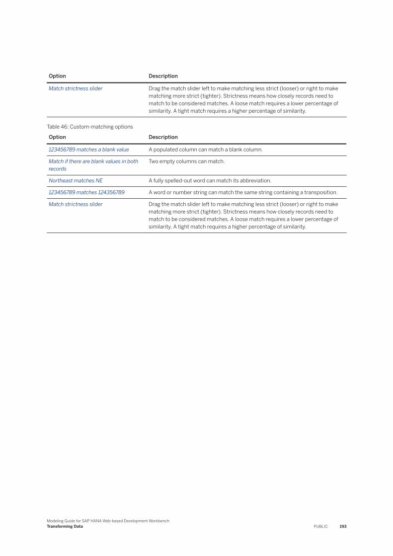
Option Description
Match strictness slider Drag the match slider left to make matching less strict (looser) or right to make matching more strict (tighter). Strictness means how closely records need to match to be considered matches. A loose match requires a lower percentage of similarity. A tight match requires a higher percentage of similarity.
Table 46: Custom-matching options
Option Description
123456789 matches a blank value A populated column can match a blank column.
Match if there are blank values in both records
Two empty columns can match.
Northeast matches NE A fully spelled-out word can match its abbreviation.
123456789 matches 124356789 A word or number string can match the same string containing a transposition.
Match strictness slider Drag the match slider left to make matching less strict (looser) or right to make matching more strict (tighter). Strictness means how closely records need to match to be considered matches. A loose match requires a lower percentage of similarity. A tight match requires a higher percentage of similarity.
Modeling Guide for SAP HANA Web-based Development WorkbenchTransforming Data PUBLIC 193

Table 47: General matching options
Option Description
Side Effect Data Level Side-effect data consists of statistics about the matching process and information about match groups and matching record pairs.
None: Side effect data is not generated.
Minimal: Generates only the statistics table that contains summary information about the matching process. The following view is created in _SYS_TASK:
● MATCH_STATISTICS
Basic: Generates the statistics table and additional views that contain information about match groups and matching record pairs. The following views are created in _SYS_TASK:
● MATCH_GROUP_INFO● MATCH_RECORD_INFO● MATCH_SOURCE_STATISTICS● MATCH_STATISTICS● MATCH_TRACING
Full: Generates the same as Basic, plus another table that contains a copy of the data in the state that it is input to the matching process. This additional view is located in the user's schema. The following views are created in _SYS_TASK:
● MATCH_GROUP_INFO● MATCH_RECORD_INFO● MATCH_SOURCE_STATISTICS● MATCH_STATISTICS● MATCH_TRACING● One side-effect user data view per Match node, containing a copy of the data
in the form that it exists as it enters the Match node
See the SAP HANA SQL and System Views Reference for information about what is contained in the side-effect views.
Source Settings Defining sources is optional and not all matching scenarios need to define sources. The two reasons for potentially wanting to define sources are to obtain statistical data per source in side effect, and to optimize performance by turning off comparisons within a source that is already free of duplicates. There are two options for defining sources.
Specify a constant source ID: All records in the input source are identified as the same source. Optionally, use a meaningful name, such as MASTER, CRM, or DELTA. If you know that a particular source is already duplicate-free, then select Do not compare within this source to prevent the unnecessary work of looking for matches that do not exist. Note that this option is available only if multiple sources are used.
Get source ID from a column: Records in the input source are a merged combination of data from different systems. A column in the data identifies which system each record originated from. Select the column that contains the identifying value.
When Match setup is complete, click Finish to close the wizard.
194 PUBLICModeling Guide for SAP HANA Web-based Development Workbench
Transforming Data

Related Information
Match Tuning Guide
5.3.19.2 Match Input Columns
Depending on the content of your data source and the columns you've chosen to output from Cleanse, these columns are automatically mapped into the Match node.
The Cleanse node generates columns containing data that is standardized and formatted to produce optimal matching results. Match input columns are automatically mapped into the Match node when all of the following conditions are met:
● Your flowgraph includes a Cleanse node.● You choose to output the Match columns from Cleanse.● You choose to use the cleansed columns in Match.
If your flowgraph does not include a Cleanse node, or if you choose not to generate those Match columns, then the Match node internally prepares the columns and uses them for finding matches.
The columns are listed alphabetically within each category.
Table 48: Person
Input column Description
MATCH_PERSON_GN Contains person name data that is prepared by the Cleanse node with the purpose of a subsequent matching process.
MATCH_PERSON_GN_STD
MATCH_PERSON_GN_STD2
MATCH_PERSON_GN_STD3
MATCH_PERSON_GN_STD4
MATCH_PERSON_GN_STD5
MATCH_PERSON_GN_STD6
MATCH_PERSON_GN2
MATCH_PERSON_GN2_STD
MATCH_PERSON_GN2_STD2
MATCH_PERSON_GN2_STD3
MATCH_PERSON_GN2_STD4
MATCH_PERSON_GN2_STD5
MATCH_PERSON_GN2_STD6
MATCH_PERSON_FN
MATCH_PERSON_FN_STD
MATCH_PERSON_MATPOST
Modeling Guide for SAP HANA Web-based Development WorkbenchTransforming Data PUBLIC 195
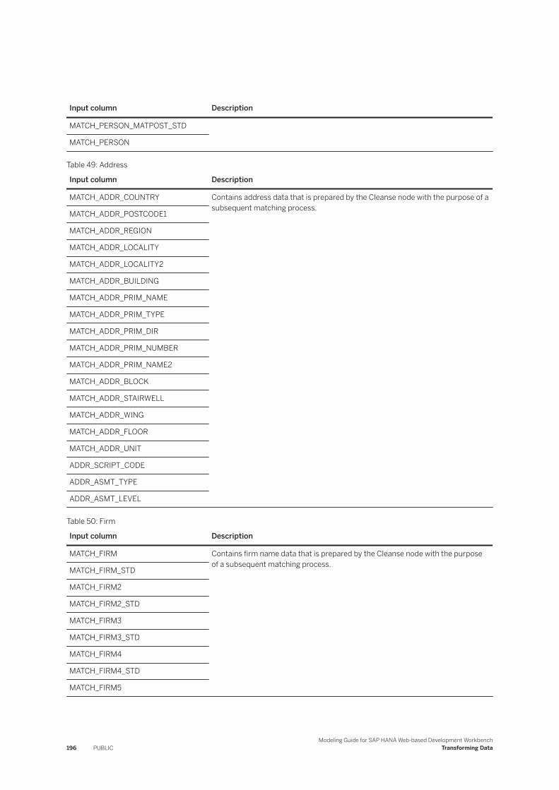
Input column Description
MATCH_PERSON_MATPOST_STD
MATCH_PERSON
Table 49: Address
Input column Description
MATCH_ADDR_COUNTRY Contains address data that is prepared by the Cleanse node with the purpose of a subsequent matching process.
MATCH_ADDR_POSTCODE1
MATCH_ADDR_REGION
MATCH_ADDR_LOCALITY
MATCH_ADDR_LOCALITY2
MATCH_ADDR_BUILDING
MATCH_ADDR_PRIM_NAME
MATCH_ADDR_PRIM_TYPE
MATCH_ADDR_PRIM_DIR
MATCH_ADDR_PRIM_NUMBER
MATCH_ADDR_PRIM_NAME2
MATCH_ADDR_BLOCK
MATCH_ADDR_STAIRWELL
MATCH_ADDR_WING
MATCH_ADDR_FLOOR
MATCH_ADDR_UNIT
ADDR_SCRIPT_CODE
ADDR_ASMT_TYPE
ADDR_ASMT_LEVEL
Table 50: Firm
Input column Description
MATCH_FIRM Contains firm name data that is prepared by the Cleanse node with the purpose of a subsequent matching process.
MATCH_FIRM_STD
MATCH_FIRM2
MATCH_FIRM2_STD
MATCH_FIRM3
MATCH_FIRM3_STD
MATCH_FIRM4
MATCH_FIRM4_STD
MATCH_FIRM5
196 PUBLICModeling Guide for SAP HANA Web-based Development Workbench
Transforming Data
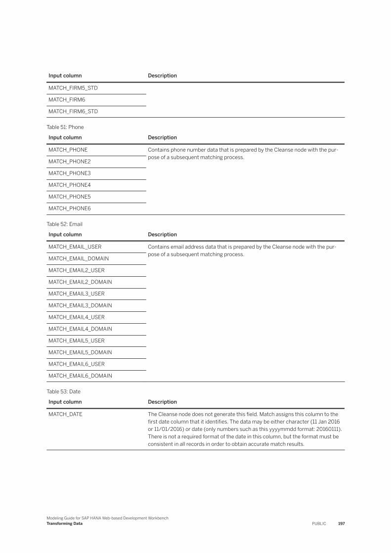
Input column Description
MATCH_FIRM5_STD
MATCH_FIRM6
MATCH_FIRM6_STD
Table 51: Phone
Input column Description
MATCH_PHONE Contains phone number data that is prepared by the Cleanse node with the purpose of a subsequent matching process.
MATCH_PHONE2
MATCH_PHONE3
MATCH_PHONE4
MATCH_PHONE5
MATCH_PHONE6
Table 52: Email
Input column Description
MATCH_EMAIL_USER Contains email address data that is prepared by the Cleanse node with the purpose of a subsequent matching process.
MATCH_EMAIL_DOMAIN
MATCH_EMAIL2_USER
MATCH_EMAIL2_DOMAIN
MATCH_EMAIL3_USER
MATCH_EMAIL3_DOMAIN
MATCH_EMAIL4_USER
MATCH_EMAIL4_DOMAIN
MATCH_EMAIL5_USER
MATCH_EMAIL5_DOMAIN
MATCH_EMAIL6_USER
MATCH_EMAIL6_DOMAIN
Table 53: Date
Input column Description
MATCH_DATE The Cleanse node does not generate this field. Match assigns this column to the first date column that it identifies. The data may be either character (11 Jan 2016 or 11/01/2016) or date (only numbers such as this yyyymmdd format: 20160111). There is not a required format of the date in this column, but the format must be consistent in all records in order to obtain accurate match results.
Modeling Guide for SAP HANA Web-based Development WorkbenchTransforming Data PUBLIC 197
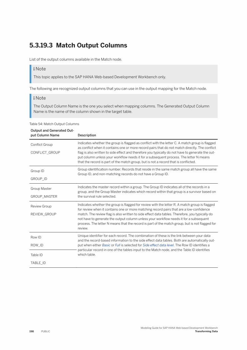
5.3.19.3 Match Output Columns
List of the output columns available in the Match node.
NoteThis topic applies to the SAP HANA Web-based Development Workbench only.
The following are recognized output columns that you can use in the output mapping for the Match node.
NoteThe Output Column Name is the one you select when mapping columns. The Generated Output Column Name is the name of the column shown in the target table.
Table 54: Match Output Columns
Output and Generated Output Column Name Description
Conflict Group
CONFLICT_GROUP
Indicates whether the group is flagged as conflict with the letter C. A match group is flagged as conflict when it contains one or more record pairs that do not match directly. The conflict flag is also written to side effect and therefore you typically do not have to generate the output column unless your workflow needs it for a subsequent process. The letter N means that the record is part of the match group, but is not a record that is conflicted.
Group ID
GROUP_ID
Group identification number. Records that reside in the same match group all have the same Group ID, and non-matching records do not have a Group ID.
Group Master
GROUP_MASTER
Indicates the master record within a group. The Group ID indicates all of the records in a group, and the Group Master indicates which record within that group is a survivor based on the survival rule selected.
Review Group
REVIEW_GROUP
Indicates whether the group is flagged for review with the letter R. A match group is flagged for review when it contains one or more matching record pairs that are a low-confidence match. The review flag is also written to side effect data tables. Therefore, you typically do not have to generate the output column unless your workflow needs it for a subsequent process. The letter N means that the record is part of the match group, but is not flagged for review.
Row ID
ROW_ID
Unique identifier for each record. The combination of these is the link between your data and the record-based information to the side effect data tables. Both are automatically output when either Basic or Full is selected for Side effect data level. The Row ID identifies a particular record in one of the tables input to the Match node, and the Table ID identifies which table.Table ID
TABLE_ID
198 PUBLICModeling Guide for SAP HANA Web-based Development Workbench
Transforming Data
5.3.20 Output Type
Output Type is used to set parameters for use in the output tables when the flowgraph is activated.
Context
Before using the Output Type node, you must have an existing table or table type created.
NoteIf you use an Input Type node and select real-time processing, you must also use the Output Type node.
Procedure
1. Drag the Output Type node into the Output Types pane of the flowgraph editor.2. In the Select an Object dialog, type the name of the object to add, or browse the object tree to select an
object, and click OK.3. Double-click the node to edit the properties.4. (Optional) Select JIT Data Preview to create a preview of the data as it would be output up to this point in
the flowgraph. All transformations from previous nodes, including the changes set in this node are shown in the preview by clicking the Data Preview icon on the canvas next to this node.
5. (Optional) You can delete one or more output columns from the output pane.6. On the Node Details General tab:
○ Kind: Indicates the type of input object, for example a table.
○ For Writer Type:○ Insert: Adds data to any existing data in the target○ Upsert: If the record is already in the table, then the data is updated. If the record does not already
exist in the table, then it is added.○ Update: Updates the existing data
7. Click Back to return to the flowgraph editor.
Modeling Guide for SAP HANA Web-based Development WorkbenchTransforming Data PUBLIC 199
5.3.21 Pivot
Creates a row of data from existing rows.
Context
NoteThis topic applies to the SAP HANA Web-based Development Workbench only.
Use this node to combine data from several rows into one row by creating new columns. A pivot table can help summarize the data by placing it in an output data set. For each unique value in a pivot axis column, it produces a column in the output data set.
NoteThe Pivot node is not available for real-time processing.
Procedure
1. (Optional) Select JIT Data Preview to create a preview of the data as it would be output up to this point in the flowgraph. All transformations from previous nodes, including the changes set in this node are shown in the preview by clicking the Data Preview icon on the canvas next to this node.
2. In the Axis tab, select the column that you want to use for the Axis attribute. This column determines which new columns are needed in the output table. At run time, a new column is created for each Pivoted Attribute and each unique axis value in the Axis Attribute.
3. In the Duplicate Value option, select First Row when you want to store the value in the first row when a duplicate is encountered. Select Abort when you want to cancel the transform process.
4. Select the + icon to enter the Axis Value and Attribute Prefix. The value of the Axis Attribute column that represents a particular set of output columns. A set of pivoted columns is generated for each Axis value. There should be one Axis value for each unique value in the Pivot Attribute. Under the Attribute Prefix, specify the text to be add to the front of the Pivot Attributes when creating new column names for the rotated data. An underscore is added automatically to separate the prefix name from the pivoted column name.
5. Click the Attributes tab to specify both pivot and non-pivot attributes.6. Under Non-Pivot Attributes, drag the input column names that will appear in the target table without
modification.7. Under Pivoted Attributes, drag the input column names whose values will be pivoted from rows into
columns. In the Default Value, enter the value stored when a rotated column has no corresponding data. The default is "null" if you do not enter a value. Do not enter a blank.
8. Click Save or Back to return to the flowgraph.
200 PUBLICModeling Guide for SAP HANA Web-based Development Workbench
Transforming Data

Example
Suppose that you have employee contact information, and you need to identify those records with missing data.
Employee_ID Contact_Type Contact_Name Contact_Address Phone
2178 emergency Shane McMillian 404 Walnut St. 555-1212
2178 home Bradly Smith 2168 Park Ave. S. 555-8168
2178 work Janet Garcia 801 Wall St. 555-7287
7532 emergency Adam Ellis 7518 Windmill Rd. 555-2165
7532 home Sarah La Fonde 2265 28th St. SW 555-1010
1298 work Ravi Rahim 801 Wall St. 555-7293
Because there are several rows for each employee, finding missing information may be difficult. Use the Pivot node to rearrange the data into a more searchable form without losing any category information. Set the properties as follows.
Option Value Notes
Non-pivot attributes Employee_ID Choose Employee_ID as a column that will not be pivoted. In this case, this ensures that this field is output in a single row.
Pivoted attributes Contact_Name
Contact_Phone
Select these two fields so the names and numbers of the contacts are output into a single row for each employee.
Default value Null Enter "Null" so that you can identify those areas that are empty.
Axis attribute Contact_Type Shows the order of the pivot.
Duplicate value First Row If a duplicate is found during processing, only the first record will be output, and processing continues. Choosing Abort causes the processing to fail.
Axis value emergency
home
work
This moves that data into additional columns. These are the values in the Contact_Type column in the source table.
Column prefix Emergency
Home
Work
This enters a prefix to the column headings. In this case, the column names will be:
● Emergency_Contact_Name● Emergency_Phone● Home_Contact_Name● Home_Phone● Work_Contact_Name● Work_Phone
The output data set includes the Employee_ID (not pivoted) and the Contact_Name and Phone fields for each pivot Axis Value (emergency, home, and work). In cases where the data is empty in the source, the Pivot node stores a null value.
The result is a single row for each employee, which you can use to search for missing contact information.
Modeling Guide for SAP HANA Web-based Development WorkbenchTransforming Data PUBLIC 201
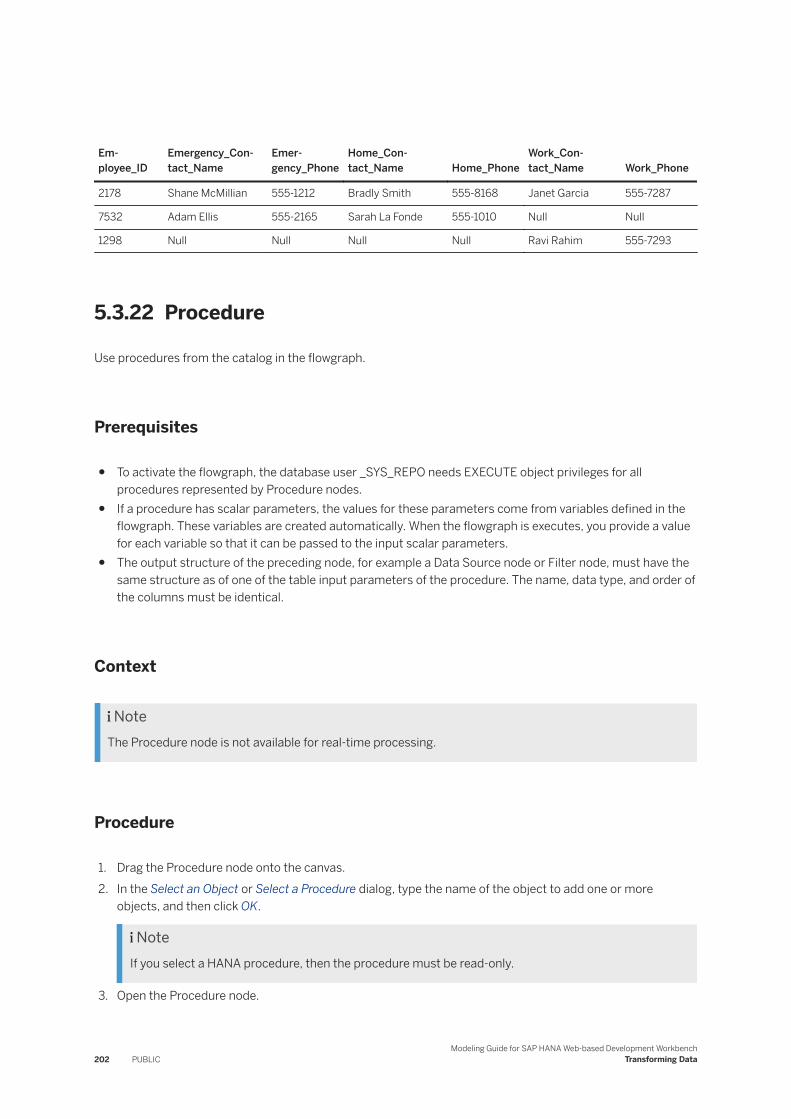
Employee_ID
Emergency_Contact_Name
Emergency_Phone
Home_Contact_Name Home_Phone
Work_Contact_Name Work_Phone
2178 Shane McMillian 555-1212 Bradly Smith 555-8168 Janet Garcia 555-7287
7532 Adam Ellis 555-2165 Sarah La Fonde 555-1010 Null Null
1298 Null Null Null Null Ravi Rahim 555-7293
5.3.22 Procedure
Use procedures from the catalog in the flowgraph.
Prerequisites
● To activate the flowgraph, the database user _SYS_REPO needs EXECUTE object privileges for all procedures represented by Procedure nodes.
● If a procedure has scalar parameters, the values for these parameters come from variables defined in the flowgraph. These variables are created automatically. When the flowgraph is executes, you provide a value for each variable so that it can be passed to the input scalar parameters.
● The output structure of the preceding node, for example a Data Source node or Filter node, must have the same structure as of one of the table input parameters of the procedure. The name, data type, and order of the columns must be identical.
Context
NoteThe Procedure node is not available for real-time processing.
Procedure
1. Drag the Procedure node onto the canvas.2. In the Select an Object or Select a Procedure dialog, type the name of the object to add one or more
objects, and then click OK.
NoteIf you select a HANA procedure, then the procedure must be read-only.
3. Open the Procedure node.
202 PUBLICModeling Guide for SAP HANA Web-based Development Workbench
Transforming Data

4. Select a Schema Name and the Procedure Name that you want to run in the flowgraphs. The schema name specifies the location and definition of the procedure.
5. Add one or more inputs to the node.6. Open the Procedure node and map the input parameters:
a. Select the parameter name in the top pane.b. On the Schema tab in the bottom pane, map each column to an Input Mapping Port Column using the
drop-down list for each column.c. Save the flowgraph.
Related Information
Using a Procedure with Scalar Output Parameters [page 203]
5.3.22.1 Using a Procedure with Scalar Output Parameters
SAP HANA procedures or virtual procedures with an output parameter as a scalar type cannot be used directly in the Procedure node.
Context
Consider the following procedure in Oracle that simply returns as output what is passed in as input:
CREATE or REPLACE PROCEDURE OUTPUT_SAME_AS_INPUT(SCALAR_IN IN VARCHAR2, SCALAR_OUT OUT VARCHAR2) IS BEGIN SCALAR_OUT := SCALAR_IN; END;
To invoke this procedure using the Procedure node, perform these steps:
Procedure
1. Create a virtual procedure that represents the procedure shown above in Oracle.
In this example, let’s assume the name of the virtual procedure is VP_OUTPUT_SAME_AS_INPUT.2. Create a procedure in SAP HANA that performs the following actions:
a. Invokes the SAP HANA procedure or virtual procedure with the scalar output.b. Puts the contents of the scalar output into the output table.
Modeling Guide for SAP HANA Web-based Development WorkbenchTransforming Data PUBLIC 203
Example
Sample Code
CREATE PROCEDURE "EXAMPLE"."SCALAR_IN_TABLE_OUT"(IN SCALAR_IN NVARCHAR(1024), OUT TABLE_OUT TABLE(SCALAR_OUT VARCHAR(1024)) AS BEGIN DECLARE SCALAR_OUT NVARCHAR(1024); CALL "VP_OUTPUT_SAME_AS_INPUT"(:SCALAR_IN, SCALAR_OUT); TABLE_OUT = SELECT :SCALAR_OUT AS SCALAR_OUT FROM DUMMY;END;
Related Information
Create a Virtual Procedure [page 13]
5.3.23 R-Script
Use the R-Script node for developing and analyzing statistical data.
R is an open-source programming language and software environment for statistical computing and graphics. The R code is embedded in SAP HANA SQL code in the form of a RLANG procedure. You can embed R-function definitions and calls within SQL Script and submit the code as part of a query to the database. You can also use R-Script to define the dataflow and schedule flowgraph processing.
NoteThe R-Script node is not available for real-time processing.
Only table types are supported in the R-Script node.
1. Place the R-Script node onto the canvas and connect the previous node. The Select Input Parameter dialog appears.
2. Choose one of the options, and then click OK.○ Select existing: select the input port name that you want to use. These inputs are predefined in the
node.○ Create new: creates an additional input port where you can enter fixed content or connect another
input port.3. Double-click the node to configure the options. The Script tab shows a predefined template where you can
enter your R-script code.4. Click the Parameters tab. The defined IN/OUT ports and whether they are connected are shown. If you
have connected this node to an upstream node, click the connected IN port to see the column information in the Attributes table.
5. (Optional) To create additional input or output ports, click Add in the Parameters table. Enter a unique name and choose whether it is an input or output port. Click OK.
204 PUBLICModeling Guide for SAP HANA Web-based Development Workbench
Transforming Data
6. (Optional) To create fixed content columns rather than using the columns from an upstream node or data source, do not connect any input source to this port, and complete these substeps.1. In the Attributes table, click Add.2. In the Name option, enter a unique column name, and choose a Data Type from the list. Depending on
the data type, you may need to enter a Length value also.3. Select the Nullable checkbox if the column can have empty values. Click OK.4. Repeat these substeps to create additional columns.5. Select the Fixed Content checkbox.6. Click the + icon to add values to each column. Repeat this step to add more rows of data.
7. After you have finished configuring the input and output ports, click Save and Back to return to the flowgraph editor.
8. Connect the output port to the next node. The Select Output Parameter dialog appears.9. In the Select existing option, choose an output port, and then click OK.
Related Information
SAP HANA R Integration Guide
5.3.24 Row Generator
Creates a table column that contains a row ID.
Context
The Row Generation operation by itself creates only one column that contains a row ID. You would typically follow it with a Query operation, with which you can add other columns or join with other tables. Then you can follow it with other operations such as join.
NoteThe Row Generation node is not available for real-time processing.
After the node is placed on the canvas, you can see the Inspect icon. This icon opens a quick view that provides a summary of the node. The information available in the quick view depends on whether the node is connected to other nodes and how the node is configured.
After the node is connected and configured, you can see this information in the quick view when available.
Icon Description
Output Columns Shows the number of output columns.
Set the following options.
Modeling Guide for SAP HANA Web-based Development WorkbenchTransforming Data PUBLIC 205
Procedure
1. Enter the row number where you want to enter the new row.2. Specify the number of the new rows to add.3. Click Close to return to the flowgraph.
5.3.25 Sort
A Sort node represents a relational sort operation.
Context
The Sort node performs a sort by one or more attributes of the input.
NoteThe Sort node is available for real-time processing.
Procedure
1. (Optional) Select JIT Data Preview to create a preview of the data as it would be output up to this point in the flowgraph. All transformations from previous nodes, including the changes set in this node are shown in the preview by clicking the Data Preview icon on the canvas next to this node.
2. In the General tab, use the Table Editor to specify the column name.3. Under Sort Order, choose Ascending when you want the smallest number first in numerical data, or when
sorting alphabetically, start with the first letter. Choose Descending when you want the largest number first in numerical data, or when sorting alphabetically, start with the last letter. It is possible to specify several columns with descending priority.
4. (Optional) Use the up and down arrows to prioritize the columns that are sorted. The higher the column in the list, the higher the priority for sorting.
5. Click Save or Back to return to the flowgraph.
206 PUBLICModeling Guide for SAP HANA Web-based Development Workbench
Transforming Data
5.3.26 Table Comparison
Compares two tables and produces the difference between them as a dataset with rows flagged as INSERT, UPDATE, or DELETE.
Context
The table comparison operation compares two datasets and produces the difference between them as a data set with rows flagged as INSERT, UPDATE, or DELETE. The operation generates an Op_Code to identify records to be inserted, deleted, or updated to synchronize the comparison table with the input table.
NoteThe input to the Table Comparison node cannot contain any LOBs, text, or shorttext attributes, even if they are not in the list of attributes being compared.
NoteThe Table Comparison node is available for real-time processing.
Procedure
1. (Optional) Select JIT Data Preview to create a preview of the data as it would be output up to this point in the flowgraph. All transformations from previous nodes, including the changes set in this node, are shown in the preview by clicking the Data Preview icon on the canvas next to this node.
2. In the Table Comparison tab, use the Comparison table option to browse to the table that you want to compare with the input table.
3. In the Generated key attribute, select a column from the comparison table where the compare attributes and primary key are placed.
4. (Optional) Create an expression in the Filter Condition option. Specifying a filter can limit the number of records that are output based on the criteria in your expression.
5. (Optional) Select Detect Deleted Rows from Comparison Table to indicate that the input table is considered a complete dataset and records in the compare table are tagged for deletion if they do not exist in the input.
6. In the Attributes tab, drag the input column names into the Compare Attributes table. If the column you are comparing contains a primary key, select True in the Primary Key column.
7. Click Save or Back to return to the flowgraph.
Related Information
Alphabetical List of Functions (SAP HANA SQL and System Views Reference)
Modeling Guide for SAP HANA Web-based Development WorkbenchTransforming Data PUBLIC 207

5.3.27 Template File
The Template File is similar to a Data Sink node and is used when you have a file that was converted using the SAP HANA smart data integration file adapter.
Context
The smart data integration File adapter is preinstalled with the Data Provisioning Agent. The File adapter converts files to the formats available for use in SAP HANA as a virtual table.
Procedure
1. Drag the Template File node onto the canvas and connect the previous node to it. You can click the magnifying glass icon to preview the existing data in the table (if any).
2. In the General tab, specify the options.3. In the Parameters tab, choose the format of the virtual table.4. Set the options for the selected format. See the "Template File Options" topic for descriptions of the
options.5. When you have finished configuring the node, select Save or Back to return to the flowgraph.
Related Information
Template File Options [page 208]
5.3.27.1 Template File Options
Description of options for the Template File node.
General
Option Description
Remote source name Name of the remote source containing the remote object.
Remote object name The name of the remote object.
208 PUBLICModeling Guide for SAP HANA Web-based Development Workbench
Transforming Data
Option Description
Name The name of the object. This could be a virtual table name.
Authoring schema Lists the system or folder where the view or table is located.
Data layout Choose from the following options.
Column: select when the file is organized based on the column name with the data values that show up under a column heading.
Row: select when the file is organized based on the data values that show up in a row. For example, if there are column headers, those will appear in a row, and the data typically under those values are listed by row.
Writer type Choose from the following options.
insert: adds new records to the output
upsert: if a record doesn't currently exist, it is inserted into a table. If the records exists, then it is updated.
update: includes additional or more current information in an existing record.
Parameters
Option Description
Format Choose from the following options.
CSV: The file uses commas (or another delimiter) to separate the data.
FIXED: The file has a specified number of characters per column.
XML: The file is in XML format.
JSON: The file is in JSON format.
Codepage (Optional) Specify the Codepage. The codepage returns a list of all supported values for codepages by querying the adapter's JVM installation, such as UTF-8.
Force Filename Pattern (Optional) Enter a prefix or postfix for the file name. For example, us_county_census_%.txt.
SecondDateFormat (Optional) Choose the default SecondDateFormat. The options use different delimiters between the year, month, and day. The hours, minutes, and sections are consistent. You can type in your own value if you prefer the day, month, year format.
TimeStampFormat (Optional) Enter the default TimeStampFormat such as hh:mm:ss.
DateFormat (Optional) Specify the default date format such as YYYY/MM/DD.
Locale (Optional) Specify the locale of the data so that it can be interpreted correctly. Query the virtual table to see the locales supported by JVM, such as de_DE. For example, the value 3,150 in the United States is a large number, whereas in Germany, the comma might indicate a decimal value.
Skip Header Lines Enter the number of header rows you have in the input data.
Modeling Guide for SAP HANA Web-based Development WorkbenchTransforming Data PUBLIC 209

Option Description
Force Directory Pattern (Optional) Enter the directory from which files and subfiles are read.
Row Delimiter Specify the Row Delimiter by choosing or entering one of the following character sequences that indicates the end of the rows in the file.
\r\n: Value for standard Microsoft Windows
\n: Value for standard UNIX
\d13\d10: Value for Microsoft Windows that provides characters as a decimal number
\x0D\x0A: Value for Microsoft Windows that provides characters as a hex number
TimeFormat (Optional) Enter the default TimeFormat.
NoteOnly one format of each type (DateFormat, TimeFormat, SecondDateFormat) is allowed per file. If you have two columns containing different formatted dates, only the first one will be recognized. The second will be VARCHAR.
Fixed format only
Option Description
RowLength The length of the entire row of data.
ColumnStartEndPosition Enter the column character start and end positions. Separate the columns with a semicolon. For example, 0-5;6-21;22-42
CSV format only
Option Description
Column Delimiter The character sequence that separates the columns in the file. You can enter an alternate character.
| (pipe)
, (comma)
; (semicolon)
210 PUBLICModeling Guide for SAP HANA Web-based Development Workbench
Transforming Data
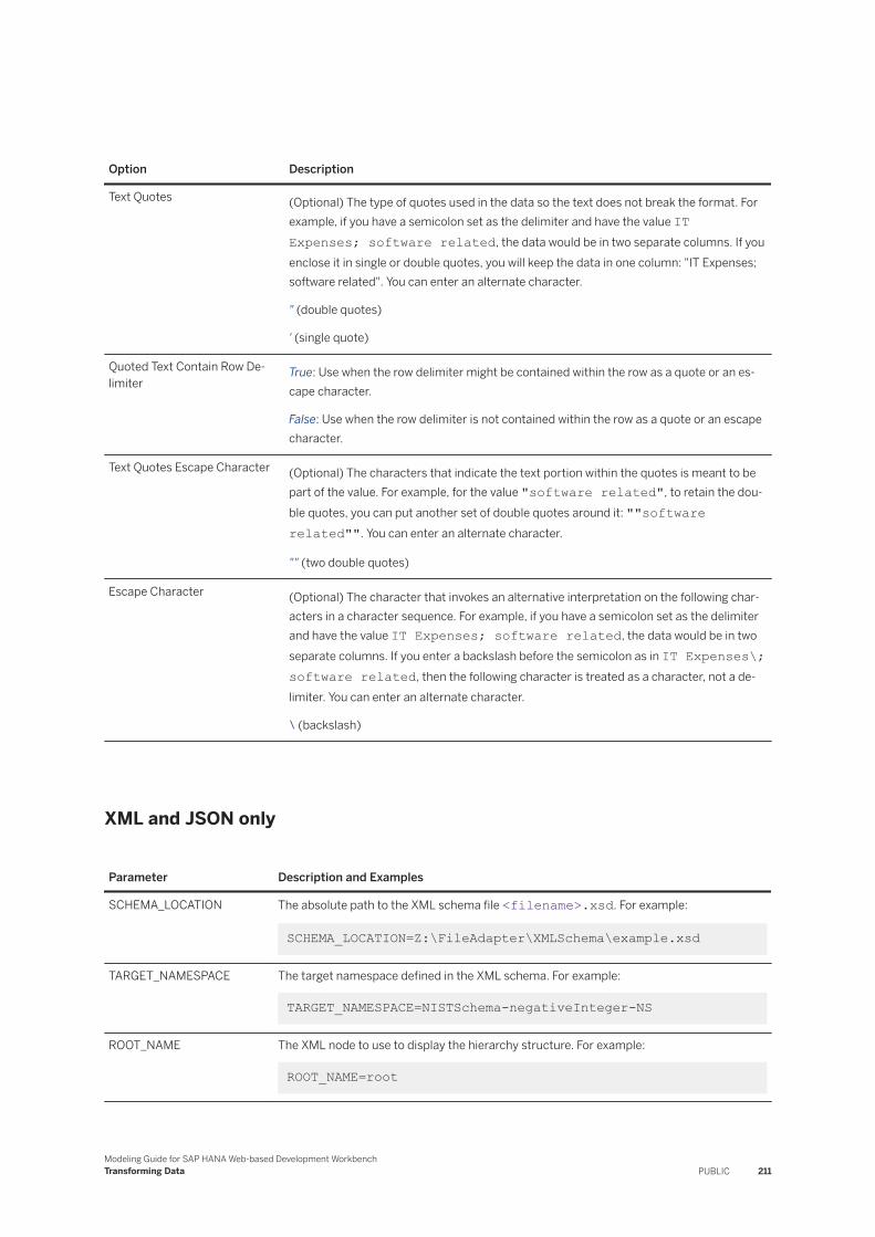
Option Description
Text Quotes (Optional) The type of quotes used in the data so the text does not break the format. For example, if you have a semicolon set as the delimiter and have the value IT Expenses; software related, the data would be in two separate columns. If you enclose it in single or double quotes, you will keep the data in one column: "IT Expenses; software related". You can enter an alternate character.
" (double quotes)
' (single quote)
Quoted Text Contain Row Delimiter
True: Use when the row delimiter might be contained within the row as a quote or an escape character.
False: Use when the row delimiter is not contained within the row as a quote or an escape character.
Text Quotes Escape Character (Optional) The characters that indicate the text portion within the quotes is meant to be part of the value. For example, for the value "software related", to retain the double quotes, you can put another set of double quotes around it: ""software related"". You can enter an alternate character.
"" (two double quotes)
Escape Character (Optional) The character that invokes an alternative interpretation on the following characters in a character sequence. For example, if you have a semicolon set as the delimiter and have the value IT Expenses; software related, the data would be in two separate columns. If you enter a backslash before the semicolon as in IT Expenses\; software related, then the following character is treated as a character, not a delimiter. You can enter an alternate character.
\ (backslash)
XML and JSON only
Parameter Description and Examples
SCHEMA_LOCATION The absolute path to the XML schema file <filename>.xsd. For example:
SCHEMA_LOCATION=Z:\FileAdapter\XMLSchema\example.xsd
TARGET_NAMESPACE The target namespace defined in the XML schema. For example:
TARGET_NAMESPACE=NISTSchema-negativeInteger-NS
ROOT_NAME The XML node to use to display the hierarchy structure. For example:
ROOT_NAME=root
Modeling Guide for SAP HANA Web-based Development WorkbenchTransforming Data PUBLIC 211

Parameter Description and Examples
CIRCULAR_LEVEL The maximum recursive level in the XML schema to display. For example:
CIRCULAR_LEVEL=3
5.3.28 Template Table
The Template Table is a generated SAP HANA table that can be used as a data target.
Context
Template tables are new tables you want to add to a database. A template table provides a quick way to generate a new target table to a flowgraph. When you use a template table, you do not have to specify the table structure or import the table metadata. Instead, during job activation, the database management system creates the table with the schema defined by the flowgraph. You can use a generated template table in a replication task.
Use template tables in the design and testing phases of your projects. You can modify the schema of the template table in the flowgraph where the table is used as a target. Any changes to the metadata require that all instances of the template table be dropped and re-added to the table.
When running a job where a template table is used as a target, use care if the table already exists because you might overwrite or change existing data. Be sure to select the correct option to insert, upsert, or update.
Procedure
1. Place the Template Table node on the canvas, and double-click to view the settings.2. (Optional) By default, your columns are mapped by name. You can change the option to map by position,
or individually remove the column mappings.
○ Map All by Position: Maps the columns by where they appear in the input and output objects.○ Map All by Name: (Default) Maps the columns by matching the column names.○ Remove Selected: Removes the column mapping of the selected column. Then, you can manually map
the input column by selecting it and dragging it on top of an unmapped output column.3. Set the following options. The History Table Settings are optional.
Tab Option Description
General Name Enter the name for the output target.
Authoring Schema Verify the schema location for the object.
212 PUBLICModeling Guide for SAP HANA Web-based Development Workbench
Transforming Data

Tab Option Description
Data Layout Specify whether to load the output data into columns or rows.
Writer Type Choose from the following:○ <blank>: Replication depends on the operation type: in
sert, update, or delete. <blank> is only available when the target has primary keys.
○ Insert: Adds data to any existing data in the target.○ Upsert: If the record is already in the table, then the
data is updated. If the record does not exist in the table, then it is added.
○ Update: Updates the existing data.
Truncate Table When enabled, the table is cleared before inserting the data during execution. When disabled, the inserted data is appended to the table during execution.
Settings Key Generation Attribute Generates new keys for target data starting from a value based on existing keys in the column you specify.
Sequence Name When generating keys, select the externally created sequence to generate the new key values.
Sequence Schema Select the schema location where you want the object.
Change Time Column Name Select the target column that is set to the time that the row was committed. The data type must be TIMESTAMP.
Change Type Column Name Select the target column that is set to the row change type. The data type is VARCHAR(1).
History Table Settings Schema Name (Optional) Select the schema location where you want the history table.
Name Enter the name for the history table.
Kind Select whether the target is a database table or a template table.
Data Layout Specify whether to load the output data in columns or rows.
4. Click Back to return to the flowgraph editor.
5.3.29 Union
A Union node represents a relational union operation.
Context
The union operator forms the union from two or more inputs with the same signature. This operator can either select all values including duplicates (UNION ALL) or only distinct values (UNION).
Modeling Guide for SAP HANA Web-based Development WorkbenchTransforming Data PUBLIC 213
NoteThe Union node is available for real-time processing.
After the node is placed on the canvas, you can see the Inspect icon. This icon opens a quick view that provides a summary of the node. The information available in the quick view depends on whether the node is connected to other nodes and how the node is configured.
After the node is connected and configured, you can see this information in the quick view when available.
Icon Description
Input Columns Shows the number of input columns.
Output Columns Shows the number of output columns.
Procedure
1. (Optional) Connect additional input sources.2. (Optional) Select Union all to merge all of the input data, including duplicate entries, into one output.3. Click Save or Back to return to the flowgraph.
5.3.30 UnPivot
Creates a new row for each value in a column identified as a pivot column.
Context
NoteThis topic applies to SAP HANA Web-based Development Workbench only.
Use this node to change how the relationship between rows is displayed. For each value in a pivot column, it produces a row in the output data set. You can create pivot sets to specify more than one pivot column.
NoteThe UnPivot node is not available for real-time processing.
214 PUBLICModeling Guide for SAP HANA Web-based Development Workbench
Transforming Data
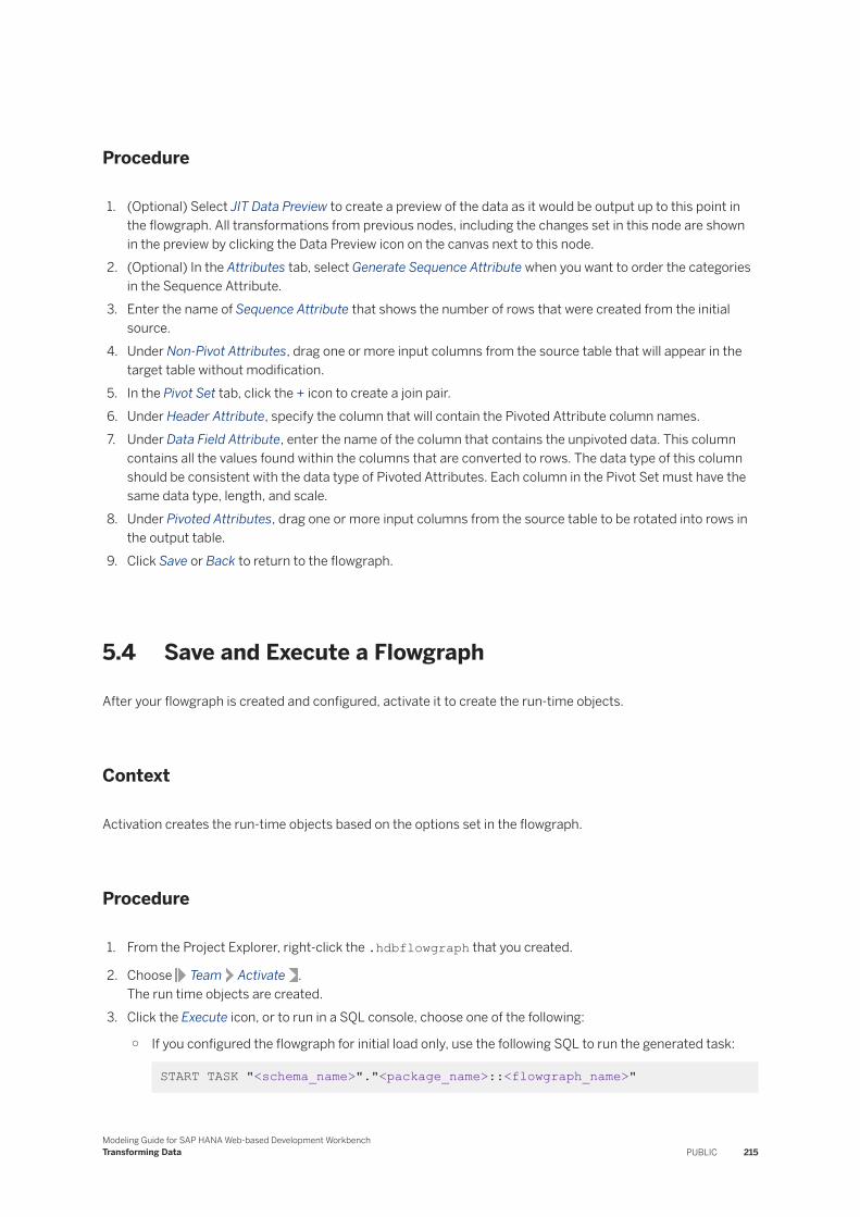
Procedure
1. (Optional) Select JIT Data Preview to create a preview of the data as it would be output up to this point in the flowgraph. All transformations from previous nodes, including the changes set in this node are shown in the preview by clicking the Data Preview icon on the canvas next to this node.
2. (Optional) In the Attributes tab, select Generate Sequence Attribute when you want to order the categories in the Sequence Attribute.
3. Enter the name of Sequence Attribute that shows the number of rows that were created from the initial source.
4. Under Non-Pivot Attributes, drag one or more input columns from the source table that will appear in the target table without modification.
5. In the Pivot Set tab, click the + icon to create a join pair.6. Under Header Attribute, specify the column that will contain the Pivoted Attribute column names.7. Under Data Field Attribute, enter the name of the column that contains the unpivoted data. This column
contains all the values found within the columns that are converted to rows. The data type of this column should be consistent with the data type of Pivoted Attributes. Each column in the Pivot Set must have the same data type, length, and scale.
8. Under Pivoted Attributes, drag one or more input columns from the source table to be rotated into rows in the output table.
9. Click Save or Back to return to the flowgraph.
5.4 Save and Execute a Flowgraph
After your flowgraph is created and configured, activate it to create the run-time objects.
Context
Activation creates the run-time objects based on the options set in the flowgraph.
Procedure
1. From the Project Explorer, right-click the .hdbflowgraph that you created.
2. Choose Team Activate .The run time objects are created.
3. Click the Execute icon, or to run in a SQL console, choose one of the following:
○ If you configured the flowgraph for initial load only, use the following SQL to run the generated task:
START TASK "<schema_name>"."<package_name>::<flowgraph_name>"
Modeling Guide for SAP HANA Web-based Development WorkbenchTransforming Data PUBLIC 215
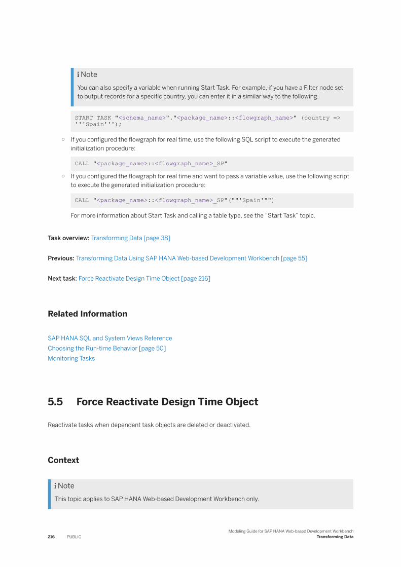
NoteYou can also specify a variable when running Start Task. For example, if you have a Filter node set to output records for a specific country, you can enter it in a similar way to the following.
START TASK "<schema_name>"."<package_name>::<flowgraph_name>" (country => '''Spain''');
○ If you configured the flowgraph for real time, use the following SQL script to execute the generated initialization procedure:
CALL "<package_name>::<flowgraph_name>_SP"
○ If you configured the flowgraph for real time and want to pass a variable value, use the following script to execute the generated initialization procedure:
CALL "<package_name>::<flowgraph_name>_SP"(""'Spain'"")
For more information about Start Task and calling a table type, see the “Start Task” topic.
Task overview: Transforming Data [page 38]
Previous: Transforming Data Using SAP HANA Web-based Development Workbench [page 55]
Next task: Force Reactivate Design Time Object [page 216]
Related Information
SAP HANA SQL and System Views ReferenceChoosing the Run-time Behavior [page 50]Monitoring Tasks
5.5 Force Reactivate Design Time Object
Reactivate tasks when dependent task objects are deleted or deactivated.
Context
NoteThis topic applies to SAP HANA Web-based Development Workbench only.
216 PUBLICModeling Guide for SAP HANA Web-based Development Workbench
Transforming Data
There might be times when an object such as a table that is used by or was generated by a flowgraph or replication task is deleted or becomes deactivated. This object might be used by more than one flowgraph or replication task. Therefore, multiple tasks might be invalid. Follow the steps below to force the reactivation of design time objects and make them active again. During force reactivation, the selected flowgraphs, replication tasks, and supporting objects are removed and recreated with the same names.
NoteYou can reactivate multiple flowgraphs and replication tasks by multi-selecting those objects that need to be reactivated. The tasks can be inside separate project containers. Only previously activated design time objects can be reactivated. If you have multi-selected several objects and don't see the Force Reactivate option, you may have included a task or object that cannot be reactivated.
Before beginning, make sure that you have the appropriate permissions to view the dependent objects using _SYS_REPO_ACTIVE_OBJECTCROSSREF. You also need permission to process the force reactivation. These are the same permissions for executing a task. See your system administrator to be assigned the appropriate permissions.
Procedure
1. From the file explorer in Web-based Development Workbench Editor, expand the Content folder. Expand your packages and select one or more flowgraph or replication tasks.
2. Right-click and select Force Reactivate.A Confirmation window shows the list of objects associated with the tasks. During processing, these objects are dropped and recreated.
NoteYou can filter on the Name, Type, or File by clicking in the column header and entering text.
3. In the Confirmation window, click Proceed.The tasks are reactivated one at a time starting from the top of the list. Tasks that are successfully reactivated are shown in the status area. Any tasks that were scheduled to reactivate after an error are not reactivated. For example, if you have four tasks to reactivate and the reactivation fails on the third task, then the third and fourth tasks are not reactivated. If the reactivation fails, an error message is shown in the status area.
If the reactivation fails, do the following:1. Refresh the file explorer. A backup file named <objectname>_<timestamp>_Backup.txt is shown
next to the original task.2. Delete the original task.3. Rename the Backup.txt file to the original flowgraph or replication task name.4. Follow the force reactivation steps again.
If nothing is displayed in the status after force reactivate has started, check the log files. Log out of Web-based Development Workbench, close the browser, and log in again to continue working.
Task overview: Transforming Data [page 38]
Modeling Guide for SAP HANA Web-based Development WorkbenchTransforming Data PUBLIC 217

Previous task: Save and Execute a Flowgraph [page 215]
Related Information
AuthorizationsActivating and Executing Task Flowgraphs and Replication Tasks
218 PUBLICModeling Guide for SAP HANA Web-based Development Workbench
Transforming Data
6 Profiling Data
You can use data profiling to examine existing data to obtain information that can improve your understanding of the makeup and type of data. The profiling capabilities in SAP HANA are semantic profiling, distribution profiling, and metadata profiling.
You access data profiling capabilities by running built-in stored procedures. These profiling stored procedures are found in the _SYS_TASK schema and are named:
● PROFILE_FREQUENCY_DISTRIBUTION● PROFILE_SEMANTIC● PROFILE_METADATA
No PUBLIC synonyms exist for the procedures, so you need to include the schema when calling the procedures.
Each profiling procedure has the following two table types associated with it that are located in the Procedures\Table Types area of the _SYS_TASK schema:
● An input table type that specifies the format for the object that includes the columns to be profiled and, in the case of distribution profiling, profiling options
● An output table type that defines the format of the stored procedure result set
Because these are built-in stored procedures, output is available only as a result set and cannot be persisted to a table even when the ‘WITH OVERVIEW’ syntax is present. The stored procedures support profiling the following types of objects:
● Column Tables● Row Tables● SQL Views● Analytic Views
NoteThis object is not supported when sampling is enabled for Semantic Profiling.
● Attribute Views● Calculation Views● Global Temporary Tables● Local Temporary Tables● Virtual Tables● Synonyms
NoteThis object is not supported when the synonym is created off of an analytic view.
Modeling Guide for SAP HANA Web-based Development WorkbenchProfiling Data PUBLIC 219
Related Information
Semantic Profiling [page 220]Distribution Profiling [page 226]Metadata Profiling [page 231]
6.1 Semantic Profiling
Semantic profiling attempts to identify the type of data in a column.
This process provides suggestions for content types based on internal evaluation of the data and metadata.
Semantic Profiling Interface
This stored procedure profiles the values of columns and returns content types that describe the possible contents of these columns.
The syntax for calling the semantic profiling stored procedure is:
CALL "_SYS_TASK"."PROFILE_SEMANTIC"('SAMPLE_SERVICES', 'PROFILE', 0, "SAMPLE_SERVICES"."SEMANTIC_PROFILING_001_COLUMNS", ?)
Or
CALL "_SYS_TASK"."PROFILE_SEMANTIC"(schema_name=>'SAMPLE_SERVICES', object_name=>'PROFILE', profile_sample=>0, columns=>"SAMPLE_SERVICES"."SEMANTIC_PROFILING_001_COLUMNS", result=>?)
Calling the stored procedure requires passing in the following parameters:
1. Schema of the object containing the data that is to be semantically profiled. For example, SAMPLE_SERVICES in the following call:
CALL "_SYS_TASK"."PROFILE_SEMANTIC"('SAMPLE_SERVICES', 'PROFILE', 0, "SAMPLE_SERVICES"."SEMANTIC_PROFILING_001_COLUMNS", ?)
2. Object that contains the data to be profiled. For example, 'PROFILE', in the following:
CALL "_SYS_TASK"."PROFILE_SEMANTIC"('SAMPLE_SERVICES', 'PROFILE', 0, "SAMPLE_SERVICES"."SEMANTIC_PROFILING_001_COLUMNS", ?)
3. Numeric value that enables (1) or disables (0) sampling functionality. Enabling sampling causes semantic profiling to occur on 1,000 random rows that are selected from the first 10,000 rows of the object to be profiled. Disabling sampling results in the semantic profiling of all rows in the object to be profiled.
NoteSampling is not supported when using semantic profiling analytic views.
220 PUBLICModeling Guide for SAP HANA Web-based Development Workbench
Profiling Data
For example, 0, in the following:
CALL "_SYS_TASK"."PROFILE_SEMANTIC"('SAMPLE_SERVICES', 'PROFILE', 0, "SAMPLE_SERVICES"."SEMANTIC_PROFILING_001_COLUMNS", ?)
4. Schema and object combination that contains the following:○ The list of columns on which semantic profiling will occur.○ Predetermined or Known Content type values, if applicable, to be considered part of the semantic
profilingFor example, "SAMPLE_SERVICES"."SEMANTIC_PROFILING_001_COLUMNS", in the following:
CALL "_SYS_TASK"."PROFILE_SEMANTIC"('SAMPLE_SERVICES', 'PROFILE', 0, "SAMPLE_SERVICES"."SEMANTIC_PROFILING_001_COLUMNS", ?)
The object passed in for this parameter must match the format of the _SYS_TASK.PROFILE_SEMANTIC_COLUMNS table type:
Column Name Data Type (Length)
COLUMN_NAME NVARCHAR (256)
SPECIFICATION_TYPE NVARCHAR(16)
SPECIFICATION_VALUE NVARCHAR(256)
The COLUMN_NAME column includes the list of column names that semantic profiling will occur on.Valid values for the SPECIFICATION_TYPE column include:
Type Description
PREDETERMINED Used when logic outside of the semantic profiling procedure has identified a potential content type that should be considered part of the semantic profiling processing.
The only supported PREDETERMINED content type is UNIQUE_ID. Passing in a PREDETERMINED UNIQUE_ID content type returns UNIQUE_ID as the winning content type when semantic profiling does not identify a more likely content type.
KNOWN_TYPE Used when the content type of a column has previously been identified and profiling of the column is not desired. Specifying this value results in the associated SPECIFICATION_VALUE content type value being:○ Used where applicable to assist in the identification of
other content types○ Presented in the profiling results
NULL
Valid values for the SPECIFICATION_VALUE column include:○ UNIQUE_ID when the SPECIFICATION_TYPE column is set to PREDETERMINED.
Modeling Guide for SAP HANA Web-based Development WorkbenchProfiling Data PUBLIC 221

○ Valid content type values when the SPECIFICATION_TYPE column is set to KNOWN_TYPE.○ NULL
The presence of a SPECIFICATION_VALUE requires a corresponding SPECIFICATION_TYPE value and vice versa.
NoteIf this object is completely empty, all columns of the object are profiled.
NoteOnly columns with the following data types return content types. Columns with data types not included below return a content type value of UNKNOWN:○ VARCHAR○ NVARCHAR○ SHORTTEXT○ ALPHANUM○ CHAR○ NCHAR○ CLOB○ NCLOB○ DATE○ TIMESTAMP○ SECONDATE
The following data types are supported only for the noted content types:○ DECIMAL (LATITUDE, LONGITUDE)○ SMALLDECIMAL (LATITUDE, LONGITUDE)○ DOUBLE (LATITUDE, LONGITUDE)○ ST_POINT (GEO_LOCATION)
5. The parameter to be used for the output result set. For example, ?, in the following:
CALL "_SYS_TASK"."PROFILE_SEMANTIC"('SAMPLE_SERVICES', 'PROFILE', 0, "SAMPLE_SERVICES"."SEMANTIC_PROFILING_001_COLUMNS", ?)
The format of the profiled output reflects the _SYS_TASK. PROFILE_SEMANTIC_RESULT table type:
Column Name Data Type (Length)
COLUMN_NAME NVARCHAR (256)
CONTENT_TYPE VARCHAR (64)
FORMAT VARCHAR (64)
SCORE DOUBLE
QUALIFIER VARCHAR (10)
222 PUBLICModeling Guide for SAP HANA Web-based Development Workbench
Profiling Data

Column Name Data Type (Length)
CONFIDENCE_RATING VARCHAR (10)
Table 55: Column name definitions
Column name Definition
COLUMN_NAME Contains from one to many instances of each column that was selected to be profiled.
CONTENT_TYPE Potential content type descriptors that can be used to describe the data.
FORMAT Provides information pertaining to the identified format of the data as it pertains to the respective content type. This is not applicable to all content types.
SCORE Internally used value to rank content types associated with a column. Scores can be normalized depending on other content type scores associated with the column, so it’s possible that two different columns that have an identical score for the same content type may return different confidence ratings.
QUALIFIER A column that is null, 'W', or 'K'.
If populated with a 'W', the semantic profiling has determined that the respective content type is the highest scoring content type, that is, the “Winning” content type.
If populated with a ‘K’, the associated content type was passed into the semantic profiling procedure as a known type.
CONFIDENCE_RATING A column that includes a text value (POOR, GOOD, VERY GOOD, EXCELLENT) that describes the confidence the noted column is of the respective content type.
Content types passed into the semantic procedure as known types have CONFIDENCE_RATING value of null.
Example
For example, we could perform semantic profiling on the following sample data, represented in the following tables:
Modeling Guide for SAP HANA Web-based Development WorkbenchProfiling Data PUBLIC 223

Table 56: SAMPLE_SERVICES.CUSTOMER_CONTACTS
COLUMN01COLUMN02
COLUMN03
COLUMN04
COLUMN05
COLUMN06
COLUMN07
COLUMN08
COLUMN09
2794387 SARAH JONES
SOFTWARE ENGINEER
ABC TECHNOLOGY INC
100 MAIN ST
MINNEAPOLIS
MN 55401 sara.jones@abctech.com
8394732 MOMOCHA KSHITRIMAYAM
RESEARCH ANALYST
ACME LIMITED
7-C BHOPAL ? ? momochak@acmelimited.com
1234890 MARY MOLITOR
PROJECT MANAGER
UNLIMITED INC
5001 FANN ST #200
CHICAGO IL 60290 mary.molitor@unlimited.org
9432872 JUAN MARTINEZ
MANAGER M&A INCORPORATED
45601 4TH AVE #5009
HENDERSON
NV 89015 pgatner.manda.org
8019759 LIZZETE SANCHEZ
PROFESSOR
MUSEO DE EL CARMEN
AV. REVOLUCION #4 Y 6
MEXICO D.F. C.P. 01000 ?
304753 MICHAEL BECKER
EDITOR STAR PUBLISHING CO
PO BOX 101 ALMONT MI 48003 [email protected]
0972398 BRIAN JACKSON
MANAGER JACKSON BUILDING SUPPLY
1001 ELM DRIVE
MARIETTA GA 30008 ?
Table 57: SAMPLE_SERVICES.CUSTOMER_CONTACTS_COLUMNS
COLUMN_NAME SPECIFICATION_TYPE SPECIFICATION_VALUE
COLUMN01 PREDETERMINED UNIQUE_ID
COLUMN02 KNOWN_TYPE NAME
COLUMN03
COLUMN04
COLUMN05
COLUMN06
COLUMN07
COLUMN08
224 PUBLICModeling Guide for SAP HANA Web-based Development Workbench
Profiling Data
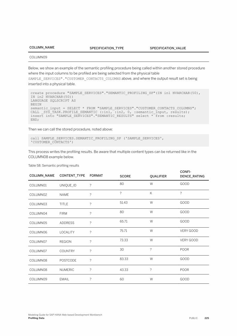
COLUMN_NAME SPECIFICATION_TYPE SPECIFICATION_VALUE
COLUMN09
Below, we show an example of the semantic profiling procedure being called within another stored procedure where the input columns to be profiled are being selected from the physical table SAMPLE_SERVICES"."CUSTOMER_CONTACTS_COLUMNS above, and where the output result set is being inserted into a physical table.
create procedure "SAMPLE_SERVICES"."SEMANTIC_PROFILING_SP"(IN in1 NVARCHAR(50), IN in2 NVARCHAR(50)) LANGUAGE SQLSCRIPT ASBEGINsemantic_input = SELECT * FROM "SAMPLE_SERVICES"."CUSTOMER_CONTACTS_COLUMNS";CALL _SYS_TASK.PROFILE_SEMANTIC (:in1, :in2, 0, :semantic_input, results);insert into "SAMPLE_SERVICES"."SEMANTIC_RESULTS" select * from :results;END;
Then we can call the stored procedure, noted above:
call SAMPLE_SERVICES.SEMANTIC_PROFILING_SP ('SAMPLE_SERVICES', 'CUSTOMER_CONTACTS')
This process writes the profiling results. Be aware that multiple content types can be returned like in the COLUMN08 example below.
Table 58: Semantic profiling results
COLUMN_NAME CONTENT_TYPE FORMAT SCORE QUALIFIERCONFIDENCE_RATING
COLUMN01 UNIQUE_ID ? 80 W GOOD
COLUMN02 NAME ? ? K ?
COLUMN03 TITLE ? 51.43 W GOOD
COLUMN04 FIRM ? 80 W GOOD
COLUMN05 ADDRESS ? 65.71 W GOOD
COLUMN06 LOCALITY ? 75.71 W VERY GOOD
COLUMN07 REGION ? 73.33 W VERY GOOD
COLUMN07 COUNTRY ? 30 ? POOR
COLUMN08 POSTCODE ? 83.33 W GOOD
COLUMN08 NUMERIC ? 43.33 ? POOR
COLUMN09 EMAIL ? 60 W GOOD
Modeling Guide for SAP HANA Web-based Development WorkbenchProfiling Data PUBLIC 225

6.2 Distribution Profiling
Distribution profiling identifies patterns, words, and values within fields.
You can perform distribution profiling on columns of data to understand the frequency of different values, words, and patterns.
The PROFILE_FREQUENCY_DISTRIBUTION procedure supports three types of distribution profiling:
Type of Distribution Profiling Description
Pattern profiling Examines string columns and normalizes the string by replacing uppercase characters, lowercase characters, and numeric characters with representative placeholders. This function keeps count of the unique computed normalized strings found for the input column.
● Uppercase characters are replaced with X.● Lowercase characters are replaced with x.● Numeric characters are replaced with 9.
After the character replacement, the function keeps count of the patterns found for the input column.
Word profiling Examines the input string and extracts words based on blank space characters as delimiters and keeps a count of unique words found in the column
Field profiling Keeps count of the all the unique column values found in the input column
The results of all three profiling types are output to a single result set.
Distribution Profiling Interface
The syntax for calling the distribution profiling procedure is:
CALL _SYS_TASK.PROFILE_FREQUENCY_DISTRIBUTION('SAMPLE_SERVICES','PROFILE',"SAMPLE_SERVICES"."PROFILE_DIST_COLUMNS",?)
Or:
CALL _SYS_TASK.PROFILE_FREQUENCY_DISTRIBUTION(schema_name=>'SAMPLE_SERVICES',object_name=>'PROFILE',columns=>"SAMPLE_SERVICES"."PROFILE_DIST_COLUMNS",result=>?)
Calling the stored procedure requires passing in four parameters:
226 PUBLICModeling Guide for SAP HANA Web-based Development Workbench
Profiling Data
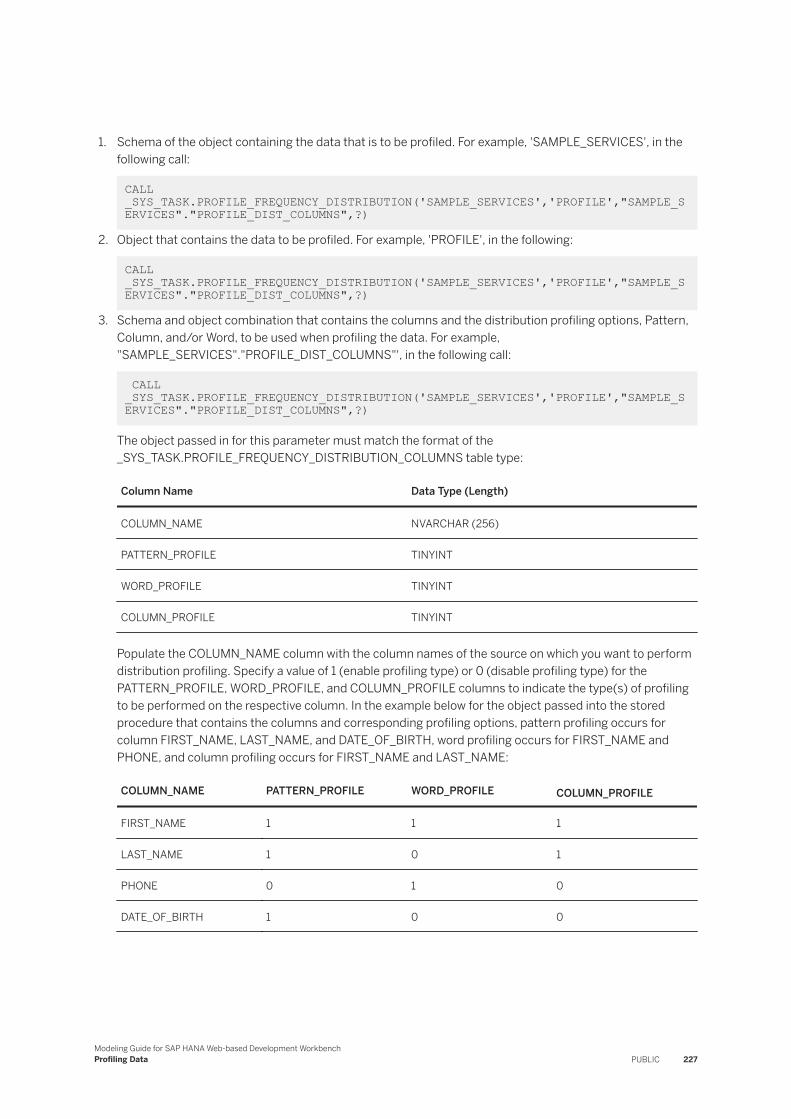
1. Schema of the object containing the data that is to be profiled. For example, 'SAMPLE_SERVICES', in the following call:
CALL _SYS_TASK.PROFILE_FREQUENCY_DISTRIBUTION('SAMPLE_SERVICES','PROFILE',"SAMPLE_SERVICES"."PROFILE_DIST_COLUMNS",?)
2. Object that contains the data to be profiled. For example, 'PROFILE', in the following:
CALL _SYS_TASK.PROFILE_FREQUENCY_DISTRIBUTION('SAMPLE_SERVICES','PROFILE',"SAMPLE_SERVICES"."PROFILE_DIST_COLUMNS",?)
3. Schema and object combination that contains the columns and the distribution profiling options, Pattern, Column, and/or Word, to be used when profiling the data. For example, "SAMPLE_SERVICES"."PROFILE_DIST_COLUMNS"', in the following call:
CALL _SYS_TASK.PROFILE_FREQUENCY_DISTRIBUTION('SAMPLE_SERVICES','PROFILE',"SAMPLE_SERVICES"."PROFILE_DIST_COLUMNS",?)
The object passed in for this parameter must match the format of the _SYS_TASK.PROFILE_FREQUENCY_DISTRIBUTION_COLUMNS table type:
Column Name Data Type (Length)
COLUMN_NAME NVARCHAR (256)
PATTERN_PROFILE TINYINT
WORD_PROFILE TINYINT
COLUMN_PROFILE TINYINT
Populate the COLUMN_NAME column with the column names of the source on which you want to perform distribution profiling. Specify a value of 1 (enable profiling type) or 0 (disable profiling type) for the PATTERN_PROFILE, WORD_PROFILE, and COLUMN_PROFILE columns to indicate the type(s) of profiling to be performed on the respective column. In the example below for the object passed into the stored procedure that contains the columns and corresponding profiling options, pattern profiling occurs for column FIRST_NAME, LAST_NAME, and DATE_OF_BIRTH, word profiling occurs for FIRST_NAME and PHONE, and column profiling occurs for FIRST_NAME and LAST_NAME:
COLUMN_NAME PATTERN_PROFILE WORD_PROFILE COLUMN_PROFILE
FIRST_NAME 1 1 1
LAST_NAME 1 0 1
PHONE 0 1 0
DATE_OF_BIRTH 1 0 0
Modeling Guide for SAP HANA Web-based Development WorkbenchProfiling Data PUBLIC 227
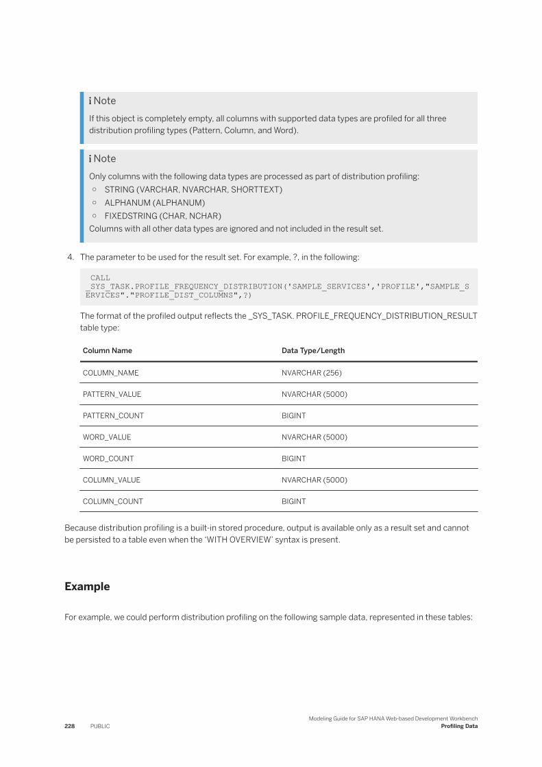
NoteIf this object is completely empty, all columns with supported data types are profiled for all three distribution profiling types (Pattern, Column, and Word).
NoteOnly columns with the following data types are processed as part of distribution profiling:○ STRING (VARCHAR, NVARCHAR, SHORTTEXT)○ ALPHANUM (ALPHANUM)○ FIXEDSTRING (CHAR, NCHAR)
Columns with all other data types are ignored and not included in the result set.
4. The parameter to be used for the result set. For example, ?, in the following:
CALL _SYS_TASK.PROFILE_FREQUENCY_DISTRIBUTION('SAMPLE_SERVICES','PROFILE',"SAMPLE_SERVICES"."PROFILE_DIST_COLUMNS",?)
The format of the profiled output reflects the _SYS_TASK. PROFILE_FREQUENCY_DISTRIBUTION_RESULT table type:
Column Name Data Type/Length
COLUMN_NAME NVARCHAR (256)
PATTERN_VALUE NVARCHAR (5000)
PATTERN_COUNT BIGINT
WORD_VALUE NVARCHAR (5000)
WORD_COUNT BIGINT
COLUMN_VALUE NVARCHAR (5000)
COLUMN_COUNT BIGINT
Because distribution profiling is a built-in stored procedure, output is available only as a result set and cannot be persisted to a table even when the ‘WITH OVERVIEW’ syntax is present.
Example
For example, we could perform distribution profiling on the following sample data, represented in these tables:
228 PUBLICModeling Guide for SAP HANA Web-based Development Workbench
Profiling Data
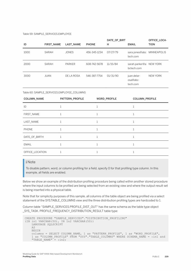
Table 59: SAMPLE_SERVICES.EMPLOYEE
ID FIRST_NAME LAST_NAME PHONEDATE_OF_BIRTH EMAIL
OFFICE_LOCATION
1000 SARAH JONES 456-345-1234 07/27/79 [email protected]
MINNEAPOLIS
2000 SARAH PARKER 608-742-5678 11/15/84 [email protected]
NEW YORK
3000 JUAN DE LA ROSA 546-387-7754 01/31/90 juan.delarosa@abctech.com
NEW YORK
Table 60: SAMPLE_SERVICES.EMPLOYEE_COLUMNS
COLUMN_NAME PATTERN_PROFILE WORD_PROFILE COLUMN_PROFILE
ID 1 1 1
FIRST_NAME 1 1 1
LAST_NAME 1 1 1
PHONE 1 1 1
DATE_OF_BIRTH 1 1 1
EMAIL 1 1 1
OFFICE_LOCATION 1 1 1
NoteTo disable pattern, word, or column profiling for a field, specify 0 for that profiling type column. In this example, all fields are enabled.
Below we show an example of the distribution profiling procedure being called within another stored procedure where the input columns to be profiled are being selected from an existing view and where the output result set is being inserted into a physical table.
Note that for simplicity purposes of this sample, all columns of the table object are being profiled via a select statement of the SYS.TABLE_COLUMNS view and the three distribution profiling types are hardcoded to 1.
Column table “SAMPLE_SERVICES.PROFILE_DIST_OUT" has the same schema as the table type object _SYS_TASK. PROFILE_FREQUENCY_DISTRIBUTION_RESULT table type:
CREATE PROCEDURE "SAMPLE_SERVICES"."DISTRIBUTION_PROFILING" (IN in1 VARCHAR(50), IN in2 VARCHAR(50)) LANGUAGE SQLSCRIPT AS BEGIN columns = SELECT COLUMN_NAME, 1 as "PATTERN_PROFILE", 1 as "WORD_PROFILE", 1 as "COLUMN_PROFILE" FROM "SYS"."TABLE_COLUMNS" WHERE SCHEMA_NAME = :in1 and "TABLE_NAME" = :in2;
Modeling Guide for SAP HANA Web-based Development WorkbenchProfiling Data PUBLIC 229
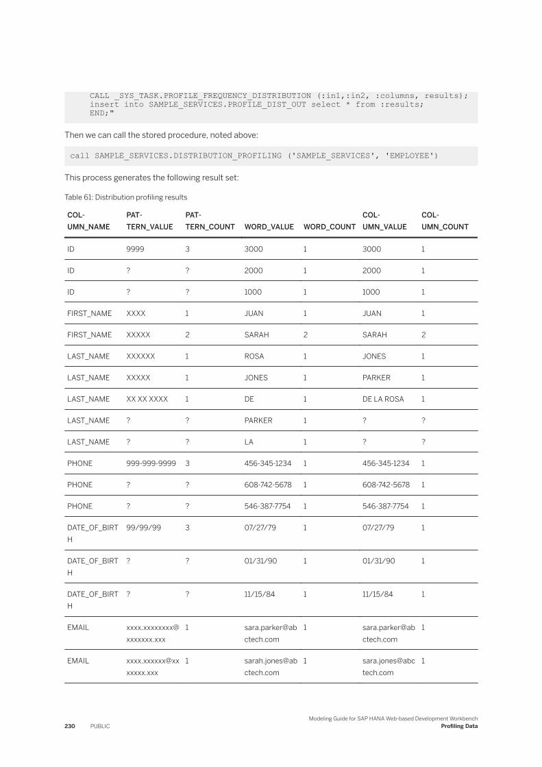
CALL _SYS_TASK.PROFILE_FREQUENCY_DISTRIBUTION (:in1,:in2, :columns, results); insert into SAMPLE_SERVICES.PROFILE_DIST_OUT select * from :results; END;"
Then we can call the stored procedure, noted above:
call SAMPLE_SERVICES.DISTRIBUTION_PROFILING ('SAMPLE_SERVICES', 'EMPLOYEE')
This process generates the following result set:
Table 61: Distribution profiling results
COLUMN_NAME
PATTERN_VALUE
PATTERN_COUNT WORD_VALUE WORD_COUNT
COLUMN_VALUE
COLUMN_COUNT
ID 9999 3 3000 1 3000 1
ID ? ? 2000 1 2000 1
ID ? ? 1000 1 1000 1
FIRST_NAME XXXX 1 JUAN 1 JUAN 1
FIRST_NAME XXXXX 2 SARAH 2 SARAH 2
LAST_NAME XXXXXX 1 ROSA 1 JONES 1
LAST_NAME XXXXX 1 JONES 1 PARKER 1
LAST_NAME XX XX XXXX 1 DE 1 DE LA ROSA 1
LAST_NAME ? ? PARKER 1 ? ?
LAST_NAME ? ? LA 1 ? ?
PHONE 999-999-9999 3 456-345-1234 1 456-345-1234 1
PHONE ? ? 608-742-5678 1 608-742-5678 1
PHONE ? ? 546-387-7754 1 546-387-7754 1
DATE_OF_BIRTH
99/99/99 3 07/27/79 1 07/27/79 1
DATE_OF_BIRTH
? ? 01/31/90 1 01/31/90 1
DATE_OF_BIRTH
? ? 11/15/84 1 11/15/84 1
EMAIL [email protected]
1
EMAIL [email protected]
1
230 PUBLICModeling Guide for SAP HANA Web-based Development Workbench
Profiling Data

COLUMN_NAME
PATTERN_VALUE
PATTERN_COUNT WORD_VALUE WORD_COUNT
COLUMN_VALUE
COLUMN_COUNT
EMAIL [email protected]
1 juan.delarosa@abctech.com
1 juan.delarosa@abctech.com
1
OFFICE_LOCATION
XXX XXXX 2 NEW 2 NEW YORK 2
OFFICE_LOCATION
XXXXXXXXXXXX
1 YORK 2 MINNEAPOLIS 1
OFFICE_LOCATION
? ? MINNEAPOLIS 1 ? ?
6.3 Metadata Profiling
Metadata profiling looks at column names, lengths, and data types to determine the content.
Metadata profiling returns content types based on the metadata. Content types are returned based on the column name and sometimes the column data types.
Metadata Profiling Interface
This stored procedure returns content types based only on the metadata information that is provided. No data is profiled and content types are returned based on column names and, in some cases, column data types.
The syntax for calling the metadata profiling procedure is:
CALL _SYS_TASK.PROFILE_METADATA('SAMPLE_SERVICES','PROFILE',"SAMPLE_SERVICES"."PROFILE_METADATA_COLUMNS",?)
Or
CALL _SYS_TASK.PROFILE_METADATA(schema_name=>'SAMPLE_SERVICES',object_name=>'PROFILE',columns=>"SAMPLE_SERVICES"."PROFILE_METADATA_COLUMNS",result=>?)
Calling the stored procedure requires passing in four parameters:
1. Schema of the object whose columns are being used for metadata profiling. For example, 'SAMPLE_SERVICES', in the following:
CALL _SYS_TASK.PROFILE_METADATA('SAMPLE_SERVICES','PROFILE',"SAMPLE_SERVICES"."PROFILE_METADATA_COLUMNS",?)
Modeling Guide for SAP HANA Web-based Development WorkbenchProfiling Data PUBLIC 231

NoteBecause column name and/or data type information is all that is necessary to return a content type and this information is contained in the object passed in as parameter three, this first parameter value can be null or empty.
2. Object whose columns are being used for metadata profiling. For example, 'PROFILE', in the following:
CALL _SYS_TASK.PROFILE_METADATA('SAMPLE_SERVICES','PROFILE',"SAMPLE_SERVICES"."PROFILE_METADATA_COLUMNS",?)
NoteBecause column name and/or data type information is all that is necessary to return a content type and this information is contained in the object passed in as parameter three, this second parameter value can be null or empty.
Reference data that includes object name and column name combinations mapped to a content type is checked as part of processing to determine a known content type, so specifying the object name if it is available could result in enhanced content type identification.
3. Schema and object combination that contains the list of columns on which semantic profiling will occur. For example, "SAMPLE_SERVICES"."PROFILE_METADATA_COLUMNS", in the following:
CALL _SYS_TASK.PROFILE_METADATA('SAMPLE_SERVICES','PROFILE',"SAMPLE_SERVICES"."PROFILE_METADATA_COLUMNS",?)
The object passed in for this parameter must match the format of the _SYS_TASK.PROFILE_METADATA_COLUMNS table type:
Column Name Data Type/Length
COLUMN_NAME NVARCHAR (256)
DATA_TYPE_NAME VARCHAR (16)
LENGTH INTEGER
NoteThe ‘DATA_TYPE_NAME’ and ‘LENGTH’ column values can be empty or null, but the columns must be preset in the object.
4. The parameter to be used for the output result set. For example, ?, in the following:
CALL _SYS_TASK.PROFILE_METADATA('SAMPLE_SERVICES','PROFILE',"SAMPLE_SERVICES"."PROFILE_METADATA_COLUMNS",?)
The format of the profiled output reflects the _SYS_TASK. PROFILE_METADATA_RESULT table type:
232 PUBLICModeling Guide for SAP HANA Web-based Development Workbench
Profiling Data
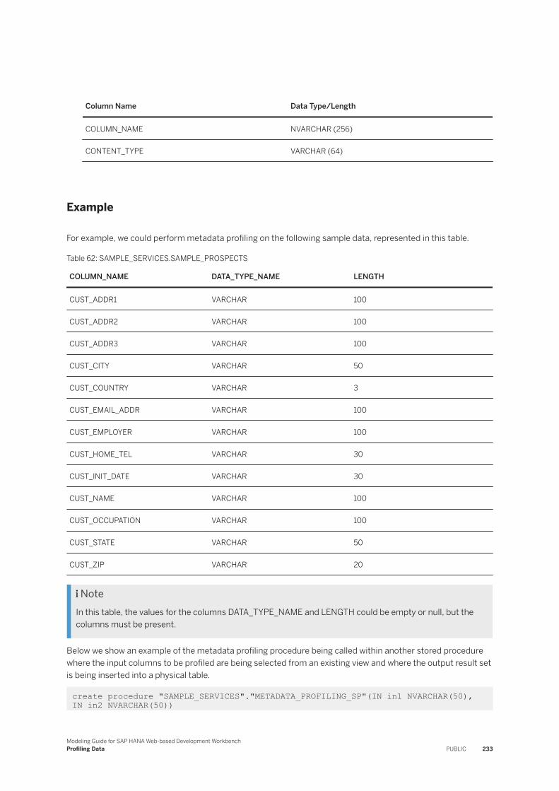
Column Name Data Type/Length
COLUMN_NAME NVARCHAR (256)
CONTENT_TYPE VARCHAR (64)
Example
For example, we could perform metadata profiling on the following sample data, represented in this table.
Table 62: SAMPLE_SERVICES.SAMPLE_PROSPECTS
COLUMN_NAME DATA_TYPE_NAME LENGTH
CUST_ADDR1 VARCHAR 100
CUST_ADDR2 VARCHAR 100
CUST_ADDR3 VARCHAR 100
CUST_CITY VARCHAR 50
CUST_COUNTRY VARCHAR 3
CUST_EMAIL_ADDR VARCHAR 100
CUST_EMPLOYER VARCHAR 100
CUST_HOME_TEL VARCHAR 30
CUST_INIT_DATE VARCHAR 30
CUST_NAME VARCHAR 100
CUST_OCCUPATION VARCHAR 100
CUST_STATE VARCHAR 50
CUST_ZIP VARCHAR 20
NoteIn this table, the values for the columns DATA_TYPE_NAME and LENGTH could be empty or null, but the columns must be present.
Below we show an example of the metadata profiling procedure being called within another stored procedure where the input columns to be profiled are being selected from an existing view and where the output result set is being inserted into a physical table.
create procedure "SAMPLE_SERVICES"."METADATA_PROFILING_SP"(IN in1 NVARCHAR(50), IN in2 NVARCHAR(50))
Modeling Guide for SAP HANA Web-based Development WorkbenchProfiling Data PUBLIC 233

LANGUAGE SQLSCRIPT ASBEGIN -- table type variable used to dynamically capture column names to be profiled metadata_input = SELECT COLUMN_NAME as "COLUMN_NAME", DATA_TYPE_NAME as "DATA_TYPE_NAME", LENGTH as "LENGTH" FROM SYS.TABLE_COLUMNS WHERE SCHEMA_NAME = :in1 and TABLE_NAME = :in2; CALL _SYS_TASK.PROFILE_METADATA (:in1, :in2, :metadata_input, results); insert into "SAMPLE_SERVICES"."METADATA_RESULTS" select * from :results; END;
Then we can call that stored procedure and pass in the object to be profiled (SAMPLE_PROSPECTS) as well as the schema in which the profiled object is contained (‘SAMPLE_SERVICES’) as follows:
call "SAMPLE_SERVICES"."METADATA_PROFILING_SP"('SAMPLE_SERVICES', 'SAMPLE_PROSPECTS')
This process writes the output result set to the table “SAMPLE_SERVICES”.”METADATA_RESULTS”.
Table 63: Metadata profiling sample results
COLUMN_NAME CONTENT_TYPE
CUST_ADDR1 ADDRESS
CUST_ADDR2 ADDRESS
CUST_ADDR3 ADDRESS
CUST_CITY LOCALITY
CUST_COUNTRY COUNTRY
CUST_EMAIL_ADDR EMAIL
CUST_EMPLOYER FIRM
CUST_HOME_TEL PHONE
CUST_INIT_DATE DATE
CUST_NAME UNKNOWN
CUST_OCCUPATION TITLE
CUST_STATE REGION
CUST_ZIP POSTCODE
234 PUBLICModeling Guide for SAP HANA Web-based Development Workbench
Profiling Data
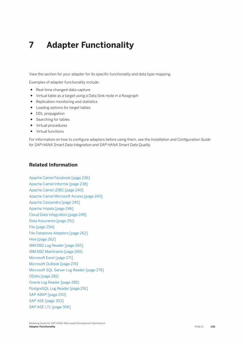
7 Adapter Functionality
View the section for your adapter for its specific functionality and data type mapping.
Examples of adapter functionality include:
● Real-time changed-data capture● Virtual table as a target using a Data Sink node in a flowgraph● Replication monitoring and statistics● Loading options for target tables● DDL propagation● Searching for tables● Virtual procedures● Virtual functions
For information on how to configure adapters before using them, see the Installation and Configuration Guide for SAP HANA Smart Data Integration and SAP HANA Smart Data Quality
Related Information
Apache Camel Facebook [page 236]Apache Camel Informix [page 238]Apache Camel JDBC [page 240]Apache Camel Microsoft Access [page 243]Apache Cassandra [page 245]Apache Impala [page 246]Cloud Data Integration [page 249]Data Assurance [page 251]File [page 254]File Datastore Adapters [page 262]Hive [page 262]IBM DB2 Log Reader [page 265]IBM DB2 Mainframe [page 269]Microsoft Excel [page 271]Microsoft Outlook [page 274]Microsoft SQL Server Log Reader [page 276]OData [page 281]Oracle Log Reader [page 285]PostgreSQL Log Reader [page 291]SAP ABAP [page 293]SAP ASE [page 303]SAP ASE LTL [page 306]
Modeling Guide for SAP HANA Web-based Development WorkbenchAdapter Functionality PUBLIC 235

SAP ECC [page 309]SAP HANA [page 312]SDI DB2 Mainframe [page 314]SOAP [page 318]Teradata [page 319]Twitter [page 324]Installation and Configuration Guide for SAP HANA Smart Data Integration and SAP HANA Smart Data QualityConfigure Data Provisioning Adapters
7.1 Apache Camel Facebook
Overview of this SAP HANA Smart Data Integration adapter’s features and functionality
The Apache Camel Facebook adapter is created based on Camel Adapter. The adapter uses the Facebook component (http://camel.apache.org/facebook.html) to access Facebook APIs. Facebook data of the configured Facebook user such as friends, families, and movies, are exposed to SAP HANA server by virtual tables by the Camel Facebook Adapter.
This adapter supports the following functionality:
● Virtual table as a source● CAP_SELECT
Related Information
Facebook Tables and Other Features [page 236]
7.1.1 Facebook Tables and Other Features
Facebook data for the configured Facebook user, such as movies, news, and so on, are exposed in SAP HANA server via virtual tables by the Camel Facebook adapter. The exposed table names and their definitions are below.
Table 64: BOOK
Column Name SQL Data Type
id VARCHAR
name VARCHAR
category VARCHAR
236 PUBLICModeling Guide for SAP HANA Web-based Development Workbench
Adapter Functionality
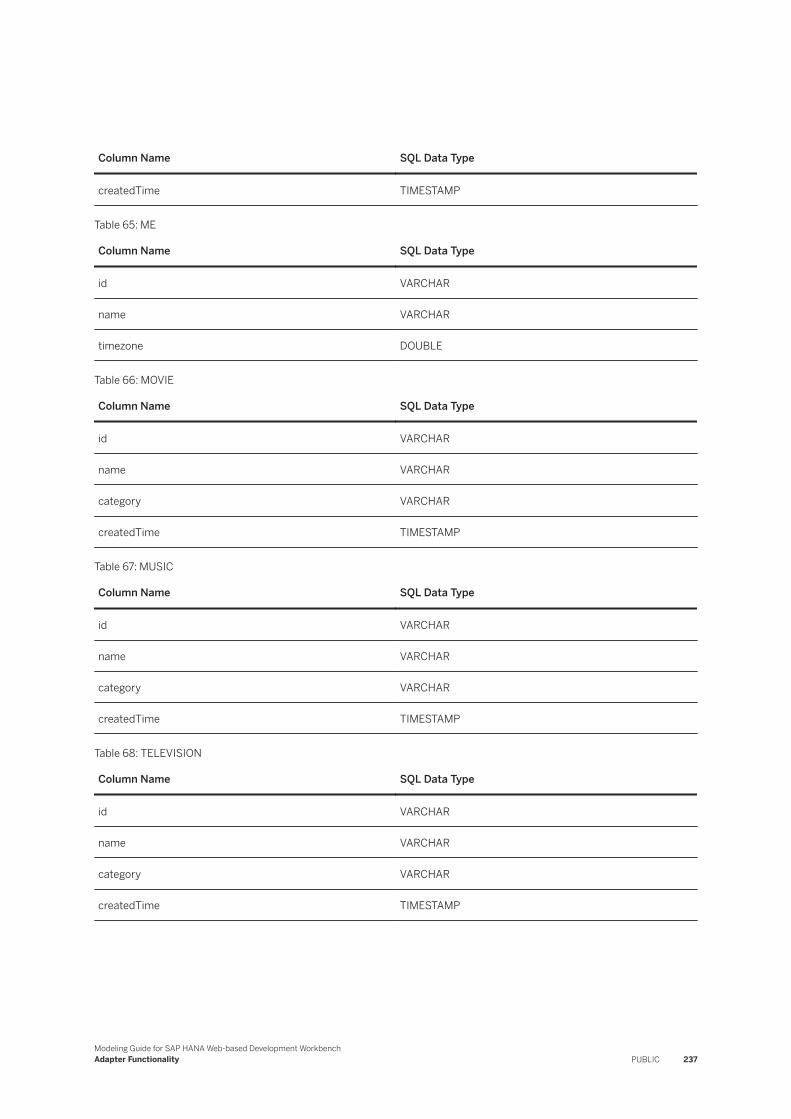
Column Name SQL Data Type
createdTime TIMESTAMP
Table 65: ME
Column Name SQL Data Type
id VARCHAR
name VARCHAR
timezone DOUBLE
Table 66: MOVIE
Column Name SQL Data Type
id VARCHAR
name VARCHAR
category VARCHAR
createdTime TIMESTAMP
Table 67: MUSIC
Column Name SQL Data Type
id VARCHAR
name VARCHAR
category VARCHAR
createdTime TIMESTAMP
Table 68: TELEVISION
Column Name SQL Data Type
id VARCHAR
name VARCHAR
category VARCHAR
createdTime TIMESTAMP
Modeling Guide for SAP HANA Web-based Development WorkbenchAdapter Functionality PUBLIC 237
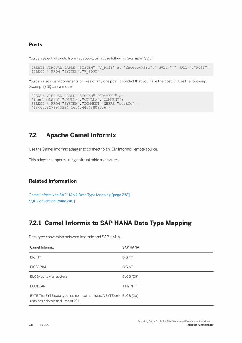
Posts
You can select all posts from Facebook, using the following (example) SQL:
CREATE VIRTUAL TABLE "SYSTEM"."V_POST" at "facebookSrc"."<NULL>"."<NULL>"."POST"; SELECT * FROM "SYSTEM"."V_POST";
You can also query comments or likes of any one post, provided that you have the post ID. Use the following (example) SQL as a model:
CREATE VIRTUAL TABLE "SYSTEM"."COMMENT" at "facebookSrc"."<NULL>"."<NULL>"."COMMENT"; SELECT * FROM "SYSTEM"."COMMENT" WHERE "postId" = '1846538278943324_1614544648809356';
7.2 Apache Camel Informix
Use the Camel Informix adapter to connect to an IBM Informix remote source.
This adapter supports using a virtual table as a source.
Related Information
Camel Informix to SAP HANA Data Type Mapping [page 238]SQL Conversion [page 240]
7.2.1 Camel Informix to SAP HANA Data Type Mapping
Data type conversion between Informix and SAP HANA.
Camel Informix SAP HANA
BIGINT BIGINT
BIGSERIAL BIGINT
BLOB (up to 4 terabytes) BLOB (2G)
BOOLEAN TINYINT
BYTE The BYTE data type has no maximum size. A BYTE column has a theoretical limit of 231
BLOB (2G)
238 PUBLICModeling Guide for SAP HANA Web-based Development Workbench
Adapter Functionality
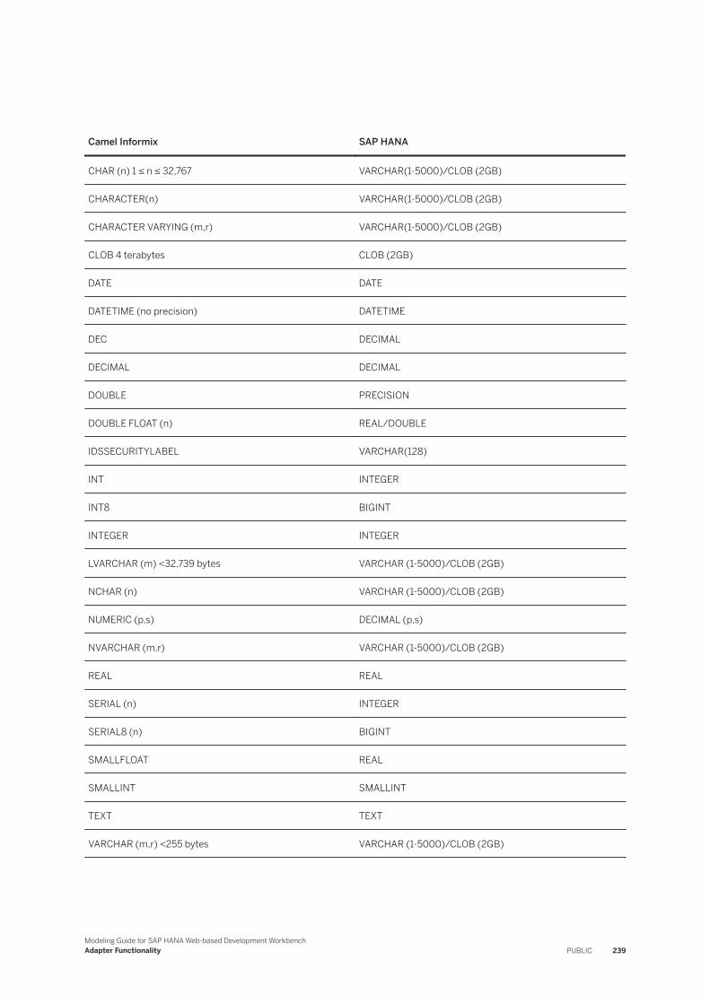
Camel Informix SAP HANA
CHAR (n) 1 ≤ n ≤ 32,767 VARCHAR(1-5000)/CLOB (2GB)
CHARACTER(n) VARCHAR(1-5000)/CLOB (2GB)
CHARACTER VARYING (m,r) VARCHAR(1-5000)/CLOB (2GB)
CLOB 4 terabytes CLOB (2GB)
DATE DATE
DATETIME (no precision) DATETIME
DEC DECIMAL
DECIMAL DECIMAL
DOUBLE PRECISION
DOUBLE FLOAT (n) REAL/DOUBLE
IDSSECURITYLABEL VARCHAR(128)
INT INTEGER
INT8 BIGINT
INTEGER INTEGER
LVARCHAR (m) <32,739 bytes VARCHAR (1-5000)/CLOB (2GB)
NCHAR (n) VARCHAR (1-5000)/CLOB (2GB)
NUMERIC (p,s) DECIMAL (p,s)
NVARCHAR (m,r) VARCHAR (1-5000)/CLOB (2GB)
REAL REAL
SERIAL (n) INTEGER
SERIAL8 (n) BIGINT
SMALLFLOAT REAL
SMALLINT SMALLINT
TEXT TEXT
VARCHAR (m,r) <255 bytes VARCHAR (1-5000)/CLOB (2GB)
Modeling Guide for SAP HANA Web-based Development WorkbenchAdapter Functionality PUBLIC 239
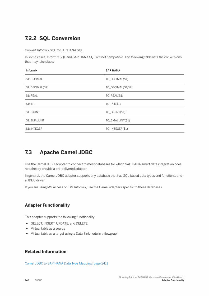
7.2.2 SQL Conversion
Convert Informix SQL to SAP HANA SQL
In some cases, Informix SQL and SAP HANA SQL are not compatible. The following table lists the conversions that may take place:
Informix SAP HANA
$1::DECIMAL TO_DECIMAL($1)
$1::DECIMAL($2) TO_DECIMAL($1,$2)
$1::REAL TO_REAL($1)
$1::INT TO_INT($1)
$1::BIGINT TO_BIGINT($1)
$1::SMALLINT TO_SMALLINT($1)
$1::INTEGER TO_INTEGER($1)
7.3 Apache Camel JDBC
Use the Camel JDBC adapter to connect to most databases for which SAP HANA smart data integration does not already provide a pre-delivered adapter.
In general, the Camel JDBC adapter supports any database that has SQL-based data types and functions, and a JDBC driver.
If you are using MS Access or IBM Informix, use the Camel adapters specific to those databases.
Adapter Functionality
This adapter supports the following functionality:
● SELECT, INSERT, UPDATE, and DELETE● Virtual table as a source● Virtual table as a target using a Data Sink node in a flowgraph
Related Information
Camel JDBC to SAP HANA Data Type Mapping [page 241]
240 PUBLICModeling Guide for SAP HANA Web-based Development Workbench
Adapter Functionality
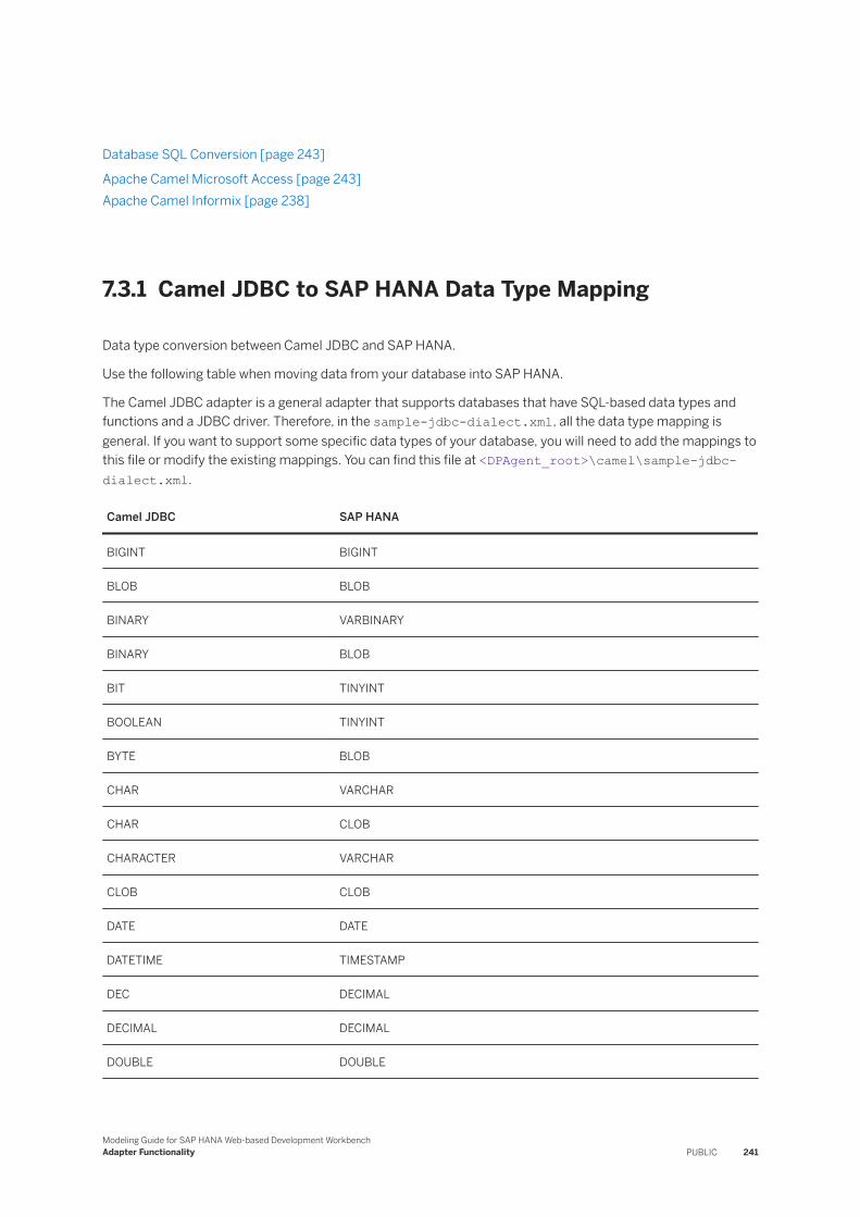
Database SQL Conversion [page 243]
Apache Camel Microsoft Access [page 243]Apache Camel Informix [page 238]
7.3.1 Camel JDBC to SAP HANA Data Type Mapping
Data type conversion between Camel JDBC and SAP HANA.
Use the following table when moving data from your database into SAP HANA.
The Camel JDBC adapter is a general adapter that supports databases that have SQL-based data types and functions and a JDBC driver. Therefore, in the sample-jdbc-dialect.xml, all the data type mapping is general. If you want to support some specific data types of your database, you will need to add the mappings to this file or modify the existing mappings. You can find this file at <DPAgent_root>\camel\sample-jdbc-dialect.xml.
Camel JDBC SAP HANA
BIGINT BIGINT
BLOB BLOB
BINARY VARBINARY
BINARY BLOB
BIT TINYINT
BOOLEAN TINYINT
BYTE BLOB
CHAR VARCHAR
CHAR CLOB
CHARACTER VARCHAR
CLOB CLOB
DATE DATE
DATETIME TIMESTAMP
DEC DECIMAL
DECIMAL DECIMAL
DOUBLE DOUBLE
Modeling Guide for SAP HANA Web-based Development WorkbenchAdapter Functionality PUBLIC 241
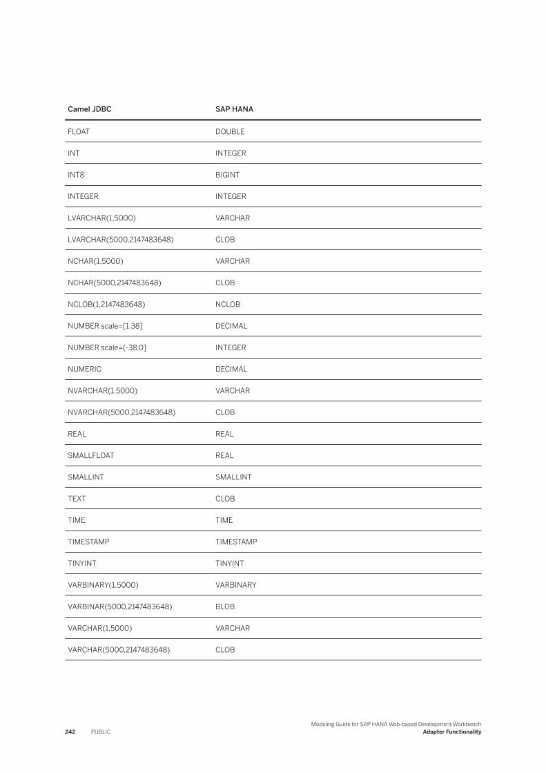
Camel JDBC SAP HANA
FLOAT DOUBLE
INT INTEGER
INT8 BIGINT
INTEGER INTEGER
LVARCHAR(1,5000) VARCHAR
LVARCHAR(5000,2147483648) CLOB
NCHAR(1,5000) VARCHAR
NCHAR(5000,2147483648) CLOB
NCLOB(1,2147483648) NCLOB
NUMBER scale=[1,38] DECIMAL
NUMBER scale=(-38,0] INTEGER
NUMERIC DECIMAL
NVARCHAR(1,5000) VARCHAR
NVARCHAR(5000,2147483648) CLOB
REAL REAL
SMALLFLOAT REAL
SMALLINT SMALLINT
TEXT CLOB
TIME TIME
TIMESTAMP TIMESTAMP
TINYINT TINYINT
VARBINARY(1,5000) VARBINARY
VARBINAR(5000,2147483648) BLOB
VARCHAR(1,5000) VARCHAR
VARCHAR(5000,2147483648) CLOB
242 PUBLICModeling Guide for SAP HANA Web-based Development Workbench
Adapter Functionality
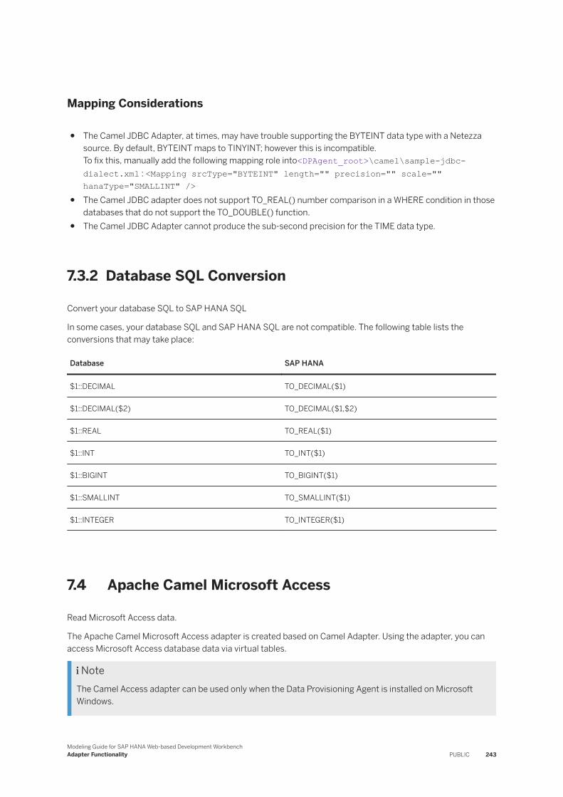
Mapping Considerations
● The Camel JDBC Adapter, at times, may have trouble supporting the BYTEINT data type with a Netezza source. By default, BYTEINT maps to TINYINT; however this is incompatible.To fix this, manually add the following mapping role into<DPAgent_root>\camel\sample-jdbc-dialect.xml : <Mapping srcType="BYTEINT" length="" precision="" scale="" hanaType="SMALLINT" />
● The Camel JDBC adapter does not support TO_REAL() number comparison in a WHERE condition in those databases that do not support the TO_DOUBLE() function.
● The Camel JDBC Adapter cannot produce the sub-second precision for the TIME data type.
7.3.2 Database SQL Conversion
Convert your database SQL to SAP HANA SQL
In some cases, your database SQL and SAP HANA SQL are not compatible. The following table lists the conversions that may take place:
Database SAP HANA
$1::DECIMAL TO_DECIMAL($1)
$1::DECIMAL($2) TO_DECIMAL($1,$2)
$1::REAL TO_REAL($1)
$1::INT TO_INT($1)
$1::BIGINT TO_BIGINT($1)
$1::SMALLINT TO_SMALLINT($1)
$1::INTEGER TO_INTEGER($1)
7.4 Apache Camel Microsoft Access
Read Microsoft Access data.
The Apache Camel Microsoft Access adapter is created based on Camel Adapter. Using the adapter, you can access Microsoft Access database data via virtual tables.
NoteThe Camel Access adapter can be used only when the Data Provisioning Agent is installed on Microsoft Windows.
Modeling Guide for SAP HANA Web-based Development WorkbenchAdapter Functionality PUBLIC 243
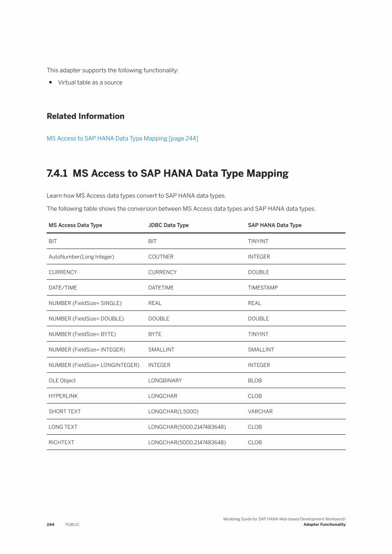
This adapter supports the following functionality:
● Virtual table as a source
Related Information
MS Access to SAP HANA Data Type Mapping [page 244]
7.4.1 MS Access to SAP HANA Data Type Mapping
Learn how MS Access data types convert to SAP HANA data types.
The following table shows the conversion between MS Access data types and SAP HANA data types.
MS Access Data Type JDBC Data Type SAP HANA Data Type
BIT BIT TINYINT
AutoNumber(Long Integer) COUTNER INTEGER
CURRENCY CURRENCY DOUBLE
DATE/TIME DATETIME TIMESTAMP
NUMBER (FieldSize= SINGLE) REAL REAL
NUMBER (FieldSize= DOUBLE) DOUBLE DOUBLE
NUMBER (FieldSize= BYTE) BYTE TINYINT
NUMBER (FieldSize= INTEGER) SMALLINT SMALLINT
NUMBER (FieldSize= LONGINTEGER) INTEGER INTEGER
OLE Object LONGBINARY BLOB
HYPERLINK LONGCHAR CLOB
SHORT TEXT LONGCHAR(1,5000) VARCHAR
LONG TEXT LONGCHAR(5000,2147483648) CLOB
RICHTEXT LONGCHAR(5000,2147483648) CLOB
244 PUBLICModeling Guide for SAP HANA Web-based Development Workbench
Adapter Functionality
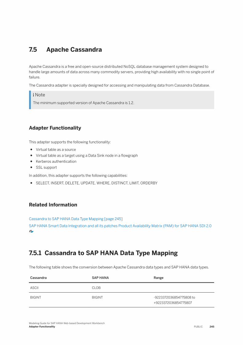
7.5 Apache Cassandra
Apache Cassandra is a free and open-source distributed NoSQL database management system designed to handle large amounts of data across many commodity servers, providing high availability with no single point of failure.
The Cassandra adapter is specially designed for accessing and manipulating data from Cassandra Database.
NoteThe minimum supported version of Apache Cassandra is 1.2.
Adapter Functionality
This adapter supports the following functionality:
● Virtual table as a source● Virtual table as a target using a Data Sink node in a flowgraph● Kerberos authentication● SSL support
In addition, this adapter supports the following capabilities:
● SELECT, INSERT, DELETE, UPDATE, WHERE, DISTINCT, LIMIT, ORDERBY
Related Information
Cassandra to SAP HANA Data Type Mapping [page 245]
SAP HANA Smart Data Integration and all its patches Product Availability Matrix (PAM) for SAP HANA SDI 2.0
7.5.1 Cassandra to SAP HANA Data Type Mapping
The following table shows the conversion between Apache Cassandra data types and SAP HANA data types.
Cassandra SAP HANA Range
ASCII CLOB
BIGINT BIGINT -9223372036854775808 to +9223372036854775807
Modeling Guide for SAP HANA Web-based Development WorkbenchAdapter Functionality PUBLIC 245
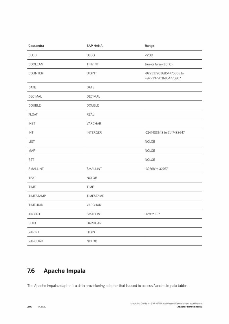
Cassandra SAP HANA Range
BLOB BLOB <2GB
BOOLEAN TINYINT true or false (1 or 0)
COUNTER BIGINT -9223372036854775808 to +9223372036854775807
DATE DATE
DECIMAL DECIMAL
DOUBLE DOUBLE
FLOAT REAL
INET VARCHAR
INT INTERGER -2147483648 to 2147483647
LIST NCLOB
MAP NCLOB
SET NCLOB
SMALLINT SMALLINT -32768 to 32767
TEXT NCLOB
TIME TIME
TIMESTAMP TIMESTAMP
TIMEUUID VARCHAR
TINYINT SMALLINT -128 to 127
UUID BARCHAR
VARINT BIGINT
VARCHAR NCLOB
7.6 Apache Impala
The Apache Impala adapter is a data provisioning adapter that is used to access Apache Impala tables.
246 PUBLICModeling Guide for SAP HANA Web-based Development Workbench
Adapter Functionality
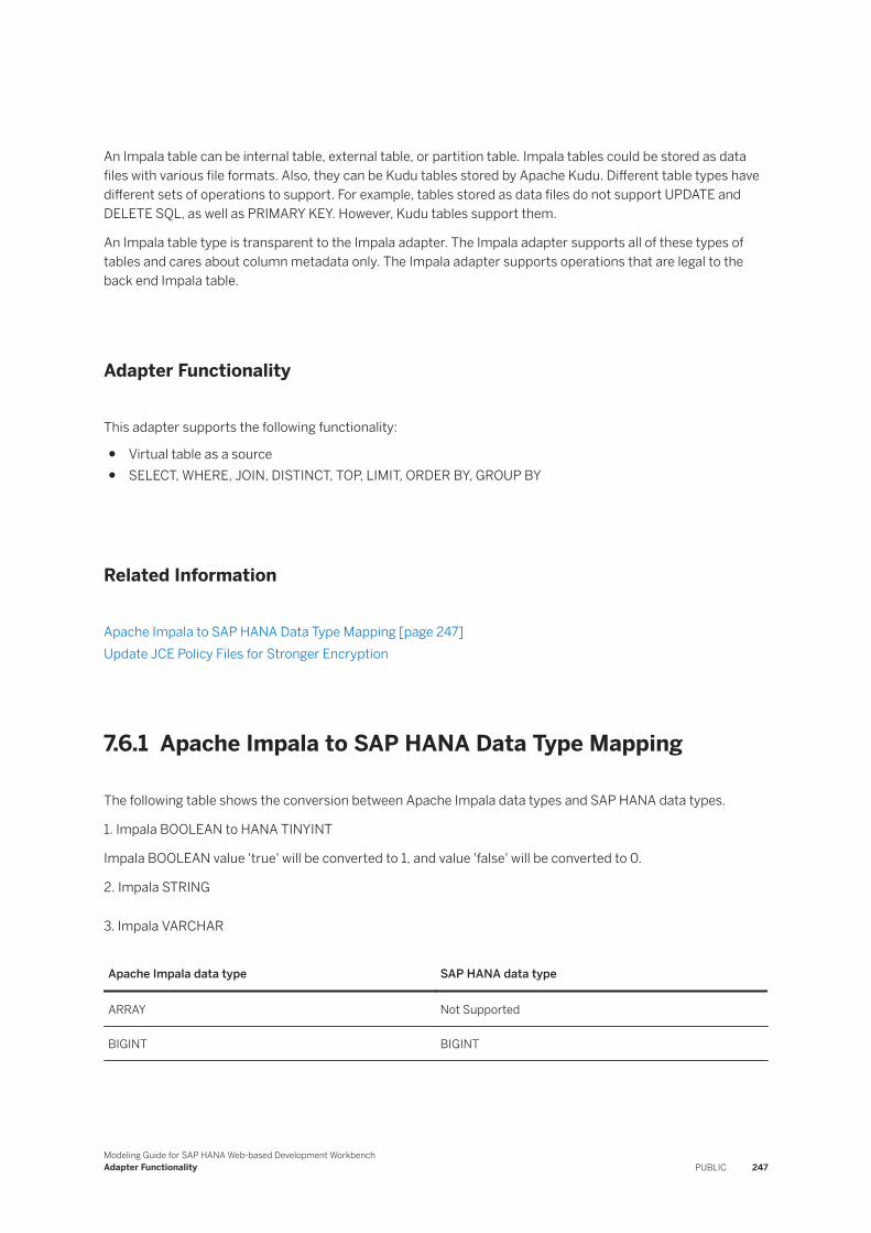
An Impala table can be internal table, external table, or partition table. Impala tables could be stored as data files with various file formats. Also, they can be Kudu tables stored by Apache Kudu. Different table types have different sets of operations to support. For example, tables stored as data files do not support UPDATE and DELETE SQL, as well as PRIMARY KEY. However, Kudu tables support them.
An Impala table type is transparent to the Impala adapter. The Impala adapter supports all of these types of tables and cares about column metadata only. The Impala adapter supports operations that are legal to the back end Impala table.
Adapter Functionality
This adapter supports the following functionality:
● Virtual table as a source● SELECT, WHERE, JOIN, DISTINCT, TOP, LIMIT, ORDER BY, GROUP BY
Related Information
Apache Impala to SAP HANA Data Type Mapping [page 247]Update JCE Policy Files for Stronger Encryption
7.6.1 Apache Impala to SAP HANA Data Type Mapping
The following table shows the conversion between Apache Impala data types and SAP HANA data types.
1. Impala BOOLEAN to HANA TINYINT
Impala BOOLEAN value 'true' will be converted to 1, and value 'false' will be converted to 0.
2. Impala STRING
3. Impala VARCHAR
Apache Impala data type SAP HANA data type
ARRAY Not Supported
BIGINT BIGINT
Modeling Guide for SAP HANA Web-based Development WorkbenchAdapter Functionality PUBLIC 247

Apache Impala data type SAP HANA data type
BOOLEAN TINYINT
NoteImpala BOOLEAN value “true” will be converted to 1, and value “false” will be converted to 0.
CHAR(n) NVARCHAR(n)
DECIMAL DECIMAL(9)
DECIMAL(p) DECIMAL(p)
DECIMAL(p,s) DECIMAL(p,s)
DOUBLE DOUBLE
FLOAT REAL
INT INTEGER
MAP Not Supported
REAL DOUBLE
SMALLINT SMALLINT
STRING CLOB
NoteImpala STRING is converted to HANA CLOB by default. Alternatively, it can be converted to HANA VARCHAR(5000), if the remote source parameter Map Impala STRING to is “VARCHAR(5000)”. In this case, exceeding trailing characters over 5000 will be stripped off.
STRUCT Not Supported
TIMESTAMP TIMESTAMP
TINYINT TINYINT
248 PUBLICModeling Guide for SAP HANA Web-based Development Workbench
Adapter Functionality
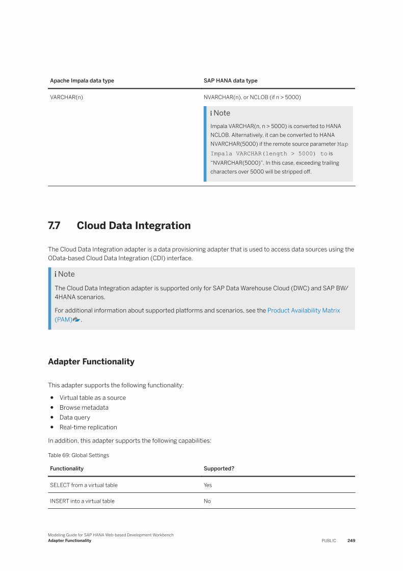
Apache Impala data type SAP HANA data type
VARCHAR(n) NVARCHAR(n), or NCLOB (if n > 5000)
NoteImpala VARCHAR(n, n > 5000) is converted to HANA NCLOB. Alternatively, it can be converted to HANA NVARCHAR(5000) if the remote source parameter Map Impala VARCHAR(length > 5000) to is “NVARCHAR(5000)”. In this case, exceeding trailing characters over 5000 will be stripped off.
7.7 Cloud Data Integration
The Cloud Data Integration adapter is a data provisioning adapter that is used to access data sources using the OData-based Cloud Data Integration (CDI) interface.
NoteThe Cloud Data Integration adapter is supported only for SAP Data Warehouse Cloud (DWC) and SAP BW/4HANA scenarios.
For additional information about supported platforms and scenarios, see the Product Availability Matrix (PAM) .
Adapter Functionality
This adapter supports the following functionality:
● Virtual table as a source● Browse metadata● Data query● Real-time replication
In addition, this adapter supports the following capabilities:
Table 69: Global Settings
Functionality Supported?
SELECT from a virtual table Yes
INSERT into a virtual table No
Modeling Guide for SAP HANA Web-based Development WorkbenchAdapter Functionality PUBLIC 249

Functionality Supported?
Execute UPDATE statements on a virtual table No
Execute DELETE statements on a virtual table No
Different capabilities per table Yes
Different capabilities per table column No
Real-time Yes, determined by the deltaEnabled annotation in the entitySet metadata
Table 70: Select Options
Functionality Supported?
Select individual columns Yes
Add a WHERE clause Yes
JOIN multiple tables No
Aggregate data via a GROUP BY clause Yes
Support a DISTINCT clause in the select No
Support a TOP or LIMIT clause in the select Yes
ORDER BY Yes
GROUP BY Yes
Related Information
Cloud Data Integration to SAP HANA Data Type Mapping [page 250]
7.7.1 Cloud Data Integration to SAP HANA Data Type Mapping
The following table shows the mapping of data types between Cloud Data Integration and SAP HANA.
OData Data Type SAP HANA Data Type
Edm.String For size <= 5000: NVARCHAR(<size>)
For size > 5000: NCLOB
250 PUBLICModeling Guide for SAP HANA Web-based Development Workbench
Adapter Functionality
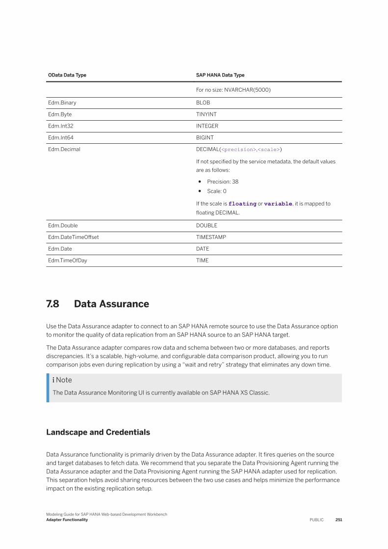
OData Data Type SAP HANA Data Type
For no size: NVARCHAR(5000)
Edm.Binary BLOB
Edm.Byte TINYINT
Edm.Int32 INTEGER
Edm.Int64 BIGINT
Edm.Decimal DECIMAL(<precision>,<scale>)
If not specified by the service metadata, the default values are as follows:
● Precision: 38● Scale: 0
If the scale is floating or variable, it is mapped to floating DECIMAL.
Edm.Double DOUBLE
Edm.DateTimeOffset TIMESTAMP
Edm.Date DATE
Edm.TimeOfDay TIME
7.8 Data Assurance
Use the Data Assurance adapter to connect to an SAP HANA remote source to use the Data Assurance option to monitor the quality of data replication from an SAP HANA source to an SAP HANA target.
The Data Assurance adapter compares row data and schema between two or more databases, and reports discrepancies. It’s a scalable, high-volume, and configurable data comparison product, allowing you to run comparison jobs even during replication by using a “wait and retry” strategy that eliminates any down time.
NoteThe Data Assurance Monitoring UI is currently available on SAP HANA XS Classic.
Landscape and Credentials
Data Assurance functionality is primarily driven by the Data Assurance adapter. It fires queries on the source and target databases to fetch data. We recommend that you separate the Data Provisioning Agent running the Data Assurance adapter and the Data Provisioning Agent running the SAP HANA adapter used for replication. This separation helps avoid sharing resources between the two use cases and helps minimize the performance impact on the existing replication setup.
Modeling Guide for SAP HANA Web-based Development WorkbenchAdapter Functionality PUBLIC 251

However, running Data Assurance on a separate Data Provisioning Agent means that the agent can’t get the credentials for the remote source from the SAP HANA database. Therefore, the remote source credentials need to be added to the Data Provisioning Agent's local secure storage, so that Data Assurance can load it as needed. You can use the agent command-line configuration tool (agentcli) to store credentials, and you can set the credentials when you configure your remote source.
Privileges for Creating a Data Assurance Adapter
If you create an adapter as a user other than SYSTEM, you need additional privileges. Run the following SQL commands for the DA_REPO1 example user:
-- Create virtual procedure and tables permission needed for data assurance adapter to create virtual objects GRANT CREATE VIRTUAL TABLE ON REMOTE SOURCE "da_repo_1" to DA_REPO1;GRANT CREATE VIRTUAL PROCEDURE ON REMOTE SOURCE "da_repo_1" to DA_REPO1; -- To create a job integrated with a subscription and fetch subscriptions and virtual tables, -- grant select for your subscription to DA user.GRANT CREATE VIRTUAL TABLE ON REMOTE SOURCE "hanaadapter1" to DA_REPO1;GRANT CREATE REMOTE SUBSCRIPTION ON REMOTE SOURCE "hanaadapter1" to DA_REPO1; -- Fetch the underlying physical tables related to subscriptions and virtual tables, -- by granting select for those tables to DA user. Grant select on the schema.GRANT SELECT ON "SYSTEM" to DA_REPO1GRANT SELECT ON "HANA_ALL_TYPE_TEST_TAB" to DA_REPO1;GRANT SELECT ON "T_HANA_ALL_TYPE_TEST_TAB_MO" to DA_REPO1;
Adapter Functionality
This adapter supports the comparison of source and target HANA tables.
NoteOnly remote subscriptions with a replication behavior of Initial + realtime or Realtime only are supported. If you use a remote subscription with other replication behaviors, the Data Assurance Monitor UI generates an error.
NoteTo ensure optimum speed and efficiency, assign Data Assurance to its own specific Data Provisioning Agent. Don’t use agent groups with Data Assurance.
Related Information
SAP HANA (Remote) to SAP HANA (Target) Data Type Mapping With Data Assurance Adapter [page 253]
252 PUBLICModeling Guide for SAP HANA Web-based Development Workbench
Adapter Functionality
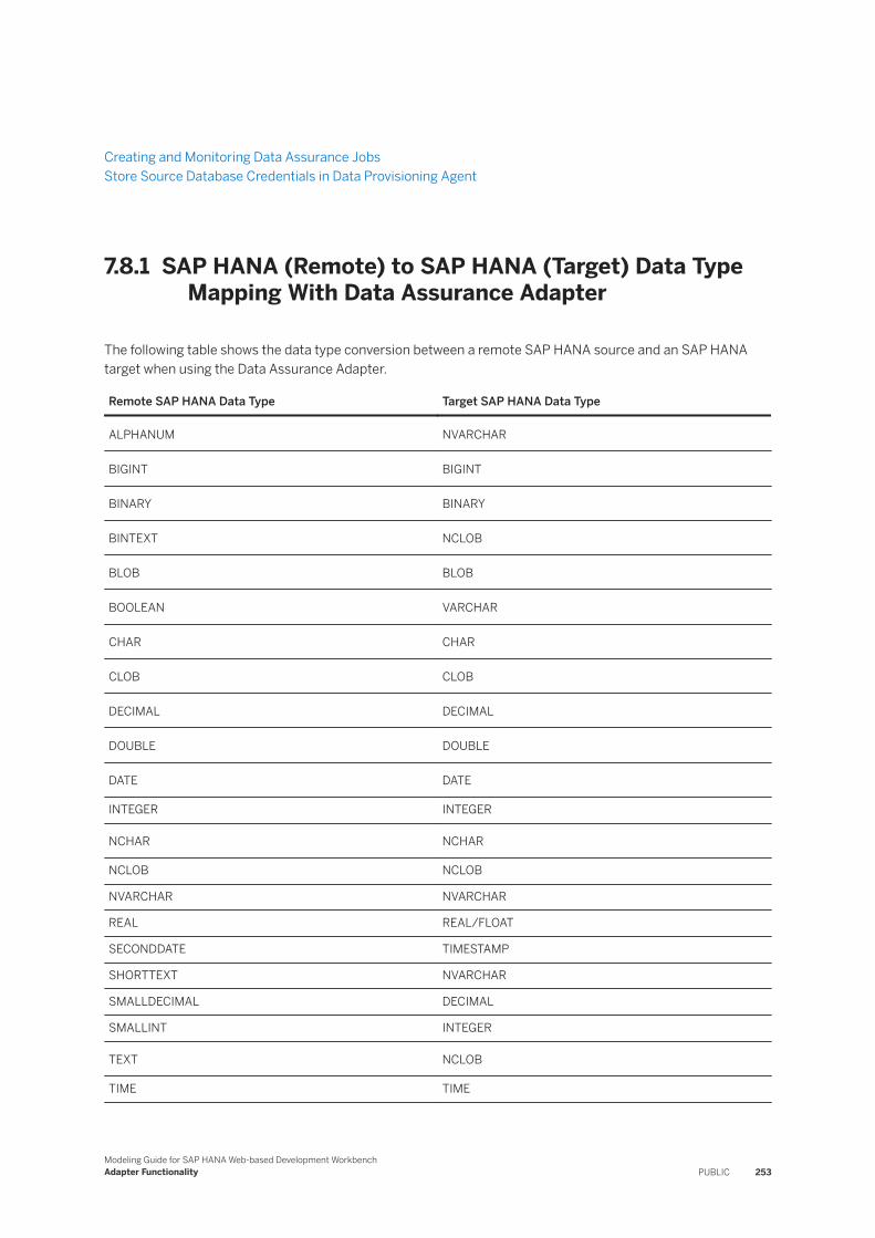
Creating and Monitoring Data Assurance JobsStore Source Database Credentials in Data Provisioning Agent
7.8.1 SAP HANA (Remote) to SAP HANA (Target) Data Type Mapping With Data Assurance Adapter
The following table shows the data type conversion between a remote SAP HANA source and an SAP HANA target when using the Data Assurance Adapter.
Remote SAP HANA Data Type Target SAP HANA Data Type
ALPHANUM NVARCHAR
BIGINT BIGINT
BINARY BINARY
BINTEXT NCLOB
BLOB BLOB
BOOLEAN VARCHAR
CHAR CHAR
CLOB CLOB
DECIMAL DECIMAL
DOUBLE DOUBLE
DATE DATE
INTEGER INTEGER
NCHAR NCHAR
NCLOB NCLOB
NVARCHAR NVARCHAR
REAL REAL/FLOAT
SECONDDATE TIMESTAMP
SHORTTEXT NVARCHAR
SMALLDECIMAL DECIMAL
SMALLINT INTEGER
TEXT NCLOB
TIME TIME
Modeling Guide for SAP HANA Web-based Development WorkbenchAdapter Functionality PUBLIC 253
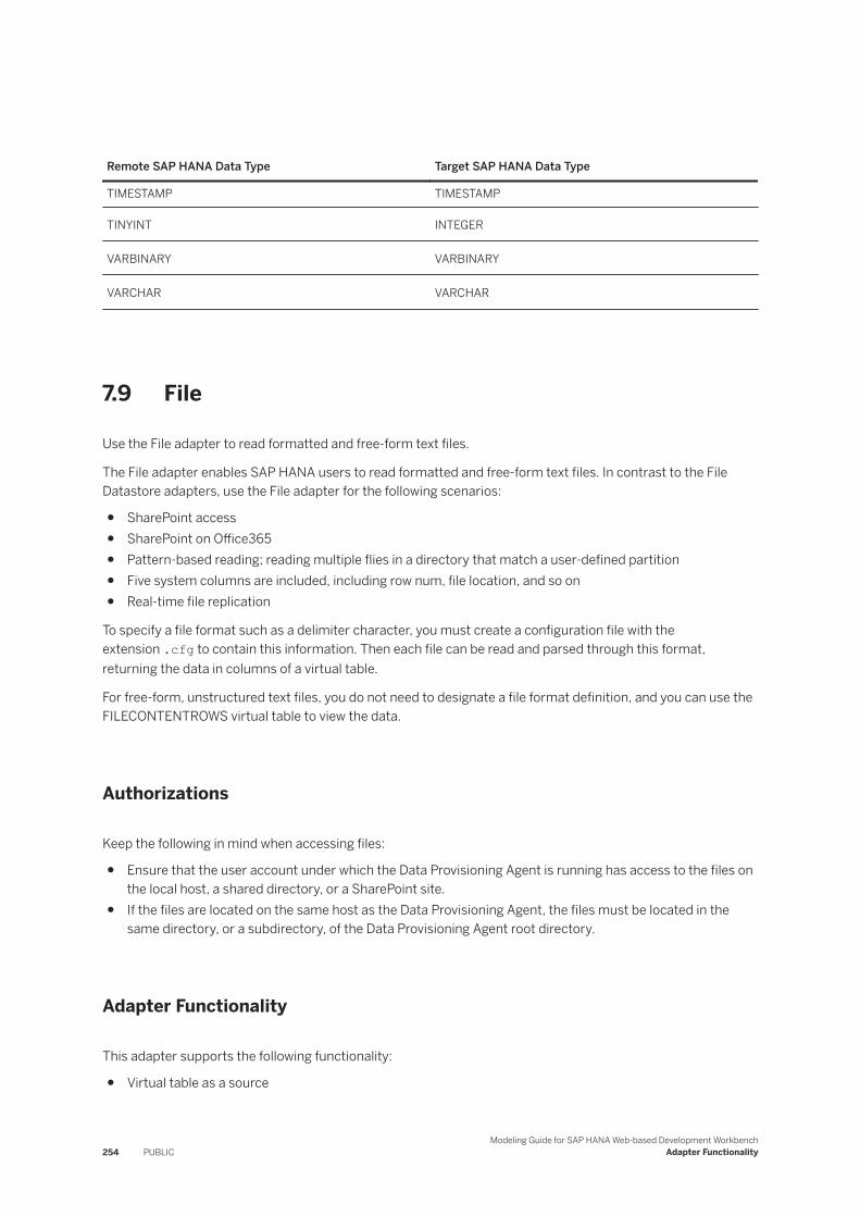
Remote SAP HANA Data Type Target SAP HANA Data Type
TIMESTAMP TIMESTAMP
TINYINT INTEGER
VARBINARY VARBINARY
VARCHAR VARCHAR
7.9 File
Use the File adapter to read formatted and free-form text files.
The File adapter enables SAP HANA users to read formatted and free-form text files. In contrast to the File Datastore adapters, use the File adapter for the following scenarios:
● SharePoint access● SharePoint on Office365● Pattern-based reading; reading multiple flies in a directory that match a user-defined partition● Five system columns are included, including row num, file location, and so on● Real-time file replication
To specify a file format such as a delimiter character, you must create a configuration file with the extension .cfg to contain this information. Then each file can be read and parsed through this format, returning the data in columns of a virtual table.
For free-form, unstructured text files, you do not need to designate a file format definition, and you can use the FILECONTENTROWS virtual table to view the data.
Authorizations
Keep the following in mind when accessing files:
● Ensure that the user account under which the Data Provisioning Agent is running has access to the files on the local host, a shared directory, or a SharePoint site.
● If the files are located on the same host as the Data Provisioning Agent, the files must be located in the same directory, or a subdirectory, of the Data Provisioning Agent root directory.
Adapter Functionality
This adapter supports the following functionality:
● Virtual table as a source
254 PUBLICModeling Guide for SAP HANA Web-based Development Workbench
Adapter Functionality

● Virtual table as a target using a Data Sink in a flowgraph; only INSERT is supported.
NoteWriting to SharePoint is not supported.
● SharePoint source support● HDFS target file support, except from SharePoint● Kerberos authentication for HDFS target files● Real-time change data capture
NoteOnly rows appended to a file initiate the capture. Only APPEND is supported. Using any other command, such as DELETE, UPDATE, and so on, may shut down replication altogether.
Also, the addition of a file to the virtual table's directory initiates the capture. This functionality is not supported for HDFS source files.
In addition, this adapter supports the following capabilities:
● SELECT, INSERT
Related Information
HDFS Target Files [page 255]Use the SFTP Virtual Procedure to Transfer Files [page 256]Call a BAT or SH File Using the EXEC Virtual Procedure [page 257]Determine the Existence of a File [page 260]Generate a Dynamic Target File Name [page 261]Writing to Multiple Files at Once [page 261]
File Datastore Adapters [page 262]
7.9.1 HDFS Target Files
You can write to an HDFS target file using the File adapter.
The File adapter supports target files copied from a local machine to a remote HDFS when processing commit changes after finishing an insert operation. You must configure your HDFS target file using the File adapter remote source configuration parameters.
An HDFS target accepts all file formats that are already supported in the File adapter.
Modeling Guide for SAP HANA Web-based Development WorkbenchAdapter Functionality PUBLIC 255
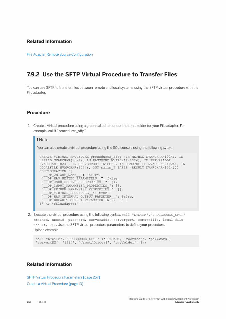
Related Information
File Adapter Remote Source Configuration
7.9.2 Use the SFTP Virtual Procedure to Transfer Files
You can use SFTP to transfer files between remote and local systems using the SFTP virtual procedure with the File adapter.
Procedure
1. Create a virtual procedure using a graphical editor, under the SFTP folder for your File adapter. For example, call it “procedures_sftp”.
NoteYou can also create a virtual procedure using the SQL console using the following sytax:
CREATE VIRTUAL PROCEDURE procedures_sftp (IN METHOD NVARCHAR(1024), IN USERID NVARCHAR(1024), IN PASSWORD NVARCHAR(1024), IN SERVERADDR NVARCHAR(1024), IN SERVERPORT INTEGER, IN REMOTEFILE NVARCHAR(1024), IN LOCALFILE NVARCHAR(1024), OUT param_7 TABLE (RESULT NVARCHAR(1024)))CONFIGURATION '{ "__DP_UNIQUE_NAME__": "SFTP", "__DP_HAS_NESTED_PARAMETERS__": false, "__DP_USER_DEFINED_PROPERTIES__": {}, "__DP_INPUT_PARAMETER_PROPERTIES_": [], "__DP_RETURN_PARAMETER_PROPERTIES_": [], "__DP_VIRTUAL_PROCEDURE__": true, "__DP_HAS_INTERNAL_OUTPUT_PARMETER__": false, "__DP_DEFAULT_OUTPUT_PARAMETER_INDEX__": 0}' AT "fileAdapter"
2. Execute the virtual procedure using the following syntax: call "SYSTEM"."PROCEDURES_SFTP" (method, userid, password, serveraddr, serverport, remotefile, local file, result, ?);. Use the SFTP virtual procedure parameters to define your procedure.Upload example
call "SYSTEM"."PROCEDURES_SFTP" ('UPLOAD', 'rootuser', 'pa$$word', "serverONE', '1234', '/root/folder1', 'c:/folder', ?);
Related Information
SFTP Virtual Procedure Parameters [page 257]
Create a Virtual Procedure [page 13]
256 PUBLICModeling Guide for SAP HANA Web-based Development Workbench
Adapter Functionality
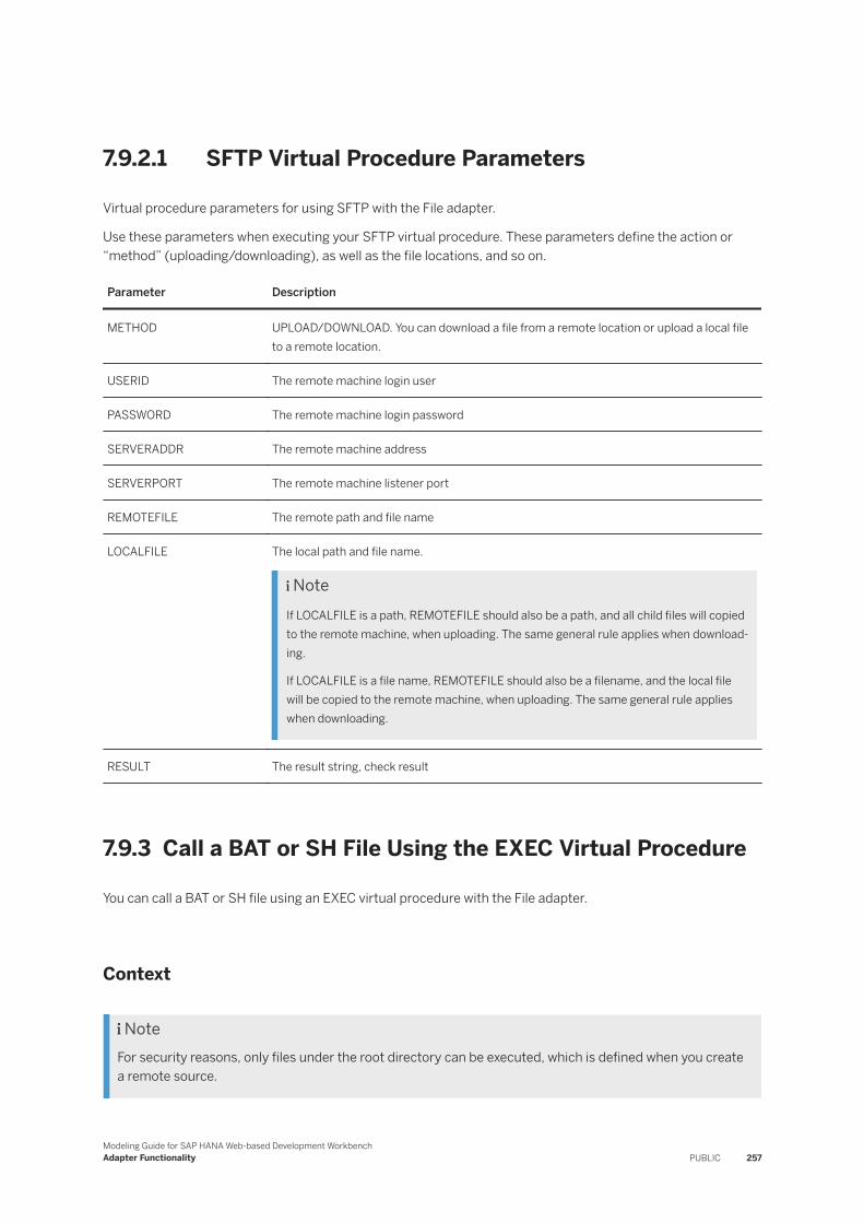
7.9.2.1 SFTP Virtual Procedure Parameters
Virtual procedure parameters for using SFTP with the File adapter.
Use these parameters when executing your SFTP virtual procedure. These parameters define the action or “method” (uploading/downloading), as well as the file locations, and so on.
Parameter Description
METHOD UPLOAD/DOWNLOAD. You can download a file from a remote location or upload a local file to a remote location.
USERID The remote machine login user
PASSWORD The remote machine login password
SERVERADDR The remote machine address
SERVERPORT The remote machine listener port
REMOTEFILE The remote path and file name
LOCALFILE The local path and file name.
NoteIf LOCALFILE is a path, REMOTEFILE should also be a path, and all child files will copied to the remote machine, when uploading. The same general rule applies when downloading.
If LOCALFILE is a file name, REMOTEFILE should also be a filename, and the local file will be copied to the remote machine, when uploading. The same general rule applies when downloading.
RESULT The result string, check result
7.9.3 Call a BAT or SH File Using the EXEC Virtual Procedure
You can call a BAT or SH file using an EXEC virtual procedure with the File adapter.
Context
NoteFor security reasons, only files under the root directory can be executed, which is defined when you create a remote source.
Modeling Guide for SAP HANA Web-based Development WorkbenchAdapter Functionality PUBLIC 257
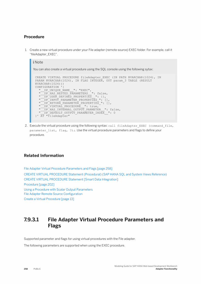
Procedure
1. Create a new virtual procedure under your File adapter (remote source) EXEC folder. For example, call it “fileAdapter_EXEC”.
NoteYou can also create a virtual procedure using the SQL console using the following sytax:
CREATE VIRTUAL PROCEDURE fileAdapter_EXEC (IN PATH NVARCHAR(1024), IN PARAM NVARCHAR(1024), IN FLAG INTEGER, OUT param_3 TABLE (RESULT NVARCHAR(1024))) CONFIGURATION '{ "__DP_UNIQUE_NAME__": "EXEC", "__DP_HAS_NESTED_PARAMETERS__": false, "__DP_USER_DEFINED_PROPERTIES__": {}, "__DP_INPUT_PARAMETER_PROPERTIES_": [], "__DP_RETURN_PARAMETER_PROPERTIES_": [], "__DP_VIRTUAL_PROCEDURE__": true, "__DP_HAS_INTERNAL_OUTPUT_PARMETER__": false, "__DP_DEFAULT_OUTPUT_PARAMETER_INDEX__": 0}' AT "fileAdapter"
2. Execute the virtual procedure using the following syntax: call fileAdapter_EXEC (command_file, parameter_list, flag, ?);. Use the virtual procedure parameters and flags to define your procedure.
Related Information
File Adapter Virtual Procedure Parameters and Flags [page 258]
CREATE VIRTUAL PROCEDURE Statement (Procedural) (SAP HANA SQL and System Views Reference)CREATE VIRTUAL PROCEDURE Statement [Smart Data Integration]Procedure [page 202]Using a Procedure with Scalar Output ParametersFile Adapter Remote Source ConfigurationCreate a Virtual Procedure [page 13]
7.9.3.1 File Adapter Virtual Procedure Parameters and Flags
Supported parameter and flags for using virtual procedures with the File adapter.
The following parameters are supported when using the EXEC procedure.
258 PUBLICModeling Guide for SAP HANA Web-based Development Workbench
Adapter Functionality
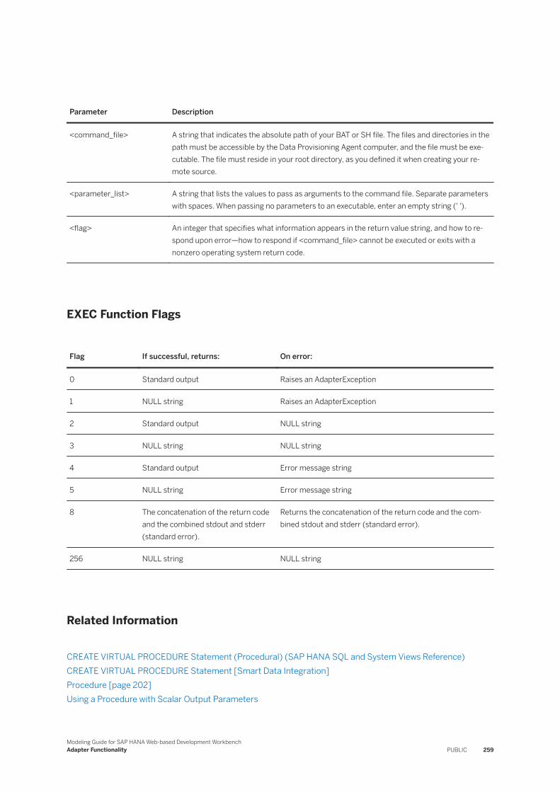
Parameter Description
<command_file> A string that indicates the absolute path of your BAT or SH file. The files and directories in the path must be accessible by the Data Provisioning Agent computer, and the file must be executable. The file must reside in your root directory, as you defined it when creating your remote source.
<parameter_list> A string that lists the values to pass as arguments to the command file. Separate parameters with spaces. When passing no parameters to an executable, enter an empty string (' ').
<flag> An integer that specifies what information appears in the return value string, and how to respond upon error—how to respond if <command_file> cannot be executed or exits with a nonzero operating system return code.
EXEC Function Flags
Flag If successful, returns: On error:
0 Standard output Raises an AdapterException
1 NULL string Raises an AdapterException
2 Standard output NULL string
3 NULL string NULL string
4 Standard output Error message string
5 NULL string Error message string
8 The concatenation of the return code and the combined stdout and stderr (standard error).
Returns the concatenation of the return code and the combined stdout and stderr (standard error).
256 NULL string NULL string
Related Information
CREATE VIRTUAL PROCEDURE Statement (Procedural) (SAP HANA SQL and System Views Reference)CREATE VIRTUAL PROCEDURE Statement [Smart Data Integration]Procedure [page 202]Using a Procedure with Scalar Output Parameters
Modeling Guide for SAP HANA Web-based Development WorkbenchAdapter Functionality PUBLIC 259

7.9.4 Determine the Existence of a File
You can use the FileExist() to determine whether a file exists in a particular directory.
Context
You may want to determine if a file exists before you perform an operation on it (read, write, and so on). To do that, use the FileExist() virtual procedure, through the File adapter.
Procedure
1. Create a virtual procedure using a graphical editor, under the FileExist folder for your File adapter. For example, call it “VP_fileAdapter_FileExist”.
2. Specify the schema, and click OK.3. Using SQL, call the virtual procedure, making sure to specify the path to location where the file may exist.
CALL "SYSTEM"."VP_fileAdapter_FileExist" (PATH => 'C:\Users\Documents\text.txt'/<VARCHAR(1023)>/,PARAM_1 => ?);
Results
A return of “1” means that the file exists in that location. A return of “0” means that the file does not exist in that location.
Related Information
Create a Virtual Procedure [page 13]
260 PUBLICModeling Guide for SAP HANA Web-based Development Workbench
Adapter Functionality
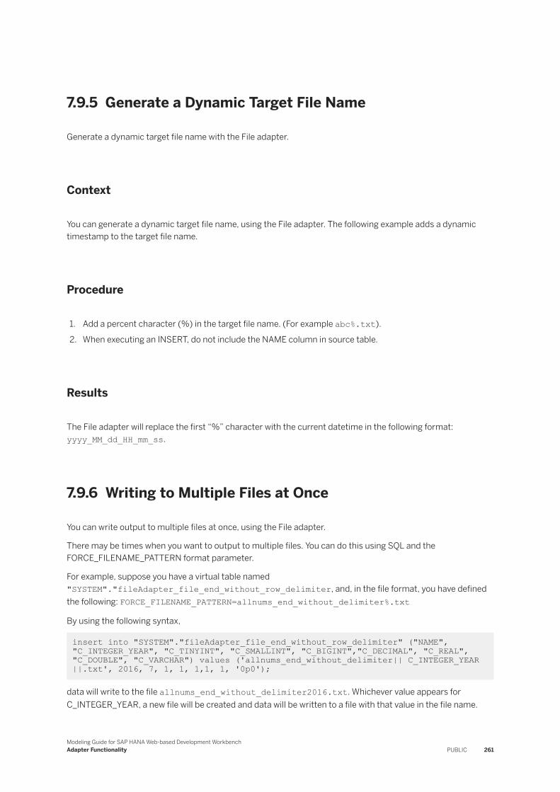
7.9.5 Generate a Dynamic Target File Name
Generate a dynamic target file name with the File adapter.
Context
You can generate a dynamic target file name, using the File adapter. The following example adds a dynamic timestamp to the target file name.
Procedure
1. Add a percent character (%) in the target file name. (For example abc%.txt).
2. When executing an INSERT, do not include the NAME column in source table.
Results
The File adapter will replace the first “%” character with the current datetime in the following format: yyyy_MM_dd_HH_mm_ss.
7.9.6 Writing to Multiple Files at Once
You can write output to multiple files at once, using the File adapter.
There may be times when you want to output to multiple files. You can do this using SQL and the FORCE_FILENAME_PATTERN format parameter.
For example, suppose you have a virtual table named "SYSTEM"."fileAdapter_file_end_without_row_delimiter, and, in the file format, you have defined the following: FORCE_FILENAME_PATTERN=allnums_end_without_delimiter%.txt
By using the following syntax,
insert into "SYSTEM"."fileAdapter_file_end_without_row_delimiter" ("NAME", "C_INTEGER_YEAR", "C_TINYINT", "C_SMALLINT", "C_BIGINT","C_DECIMAL", "C_REAL", "C_DOUBLE", "C_VARCHAR") values ('allnums_end_without_delimiter|| C_INTEGER_YEAR ||.txt', 2016, 7, 1, 1, 1,1, 1, '0p0');
data will write to the file allnums_end_without_delimiter2016.txt. Whichever value appears for C_INTEGER_YEAR, a new file will be created and data will be written to a file with that value in the file name.
Modeling Guide for SAP HANA Web-based Development WorkbenchAdapter Functionality PUBLIC 261
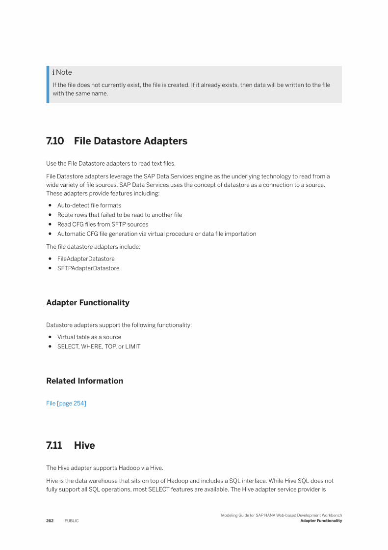
NoteIf the file does not currently exist, the file is created. If it already exists, then data will be written to the file with the same name.
7.10 File Datastore Adapters
Use the File Datastore adapters to read text files.
File Datastore adapters leverage the SAP Data Services engine as the underlying technology to read from a wide variety of file sources. SAP Data Services uses the concept of datastore as a connection to a source. These adapters provide features including:
● Auto-detect file formats● Route rows that failed to be read to another file● Read CFG files from SFTP sources● Automatic CFG file generation via virtual procedure or data file importation
The file datastore adapters include:
● FileAdapterDatastore● SFTPAdapterDatastore
Adapter Functionality
Datastore adapters support the following functionality:
● Virtual table as a source● SELECT, WHERE, TOP, or LIMIT
Related Information
File [page 254]
7.11 Hive
The Hive adapter supports Hadoop via Hive.
Hive is the data warehouse that sits on top of Hadoop and includes a SQL interface. While Hive SQL does not fully support all SQL operations, most SELECT features are available. The Hive adapter service provider is
262 PUBLICModeling Guide for SAP HANA Web-based Development Workbench
Adapter Functionality

created as a remote source, and requires the support of artifacts like virtual table and remote subscription for each source table to perform replication.
NoteBefore registering the adapter with the SAP HANA system, ensure that you have downloaded and installed the correct JDBC libraries. See the SAP HANA smart data integration Product Availability Matrix (PAM) for details. Place the files in the <DPAgent_root>/lib/hive folder.
Adapter Functionality
This adapter supports the following functionality:
● SELECT, INSERT, UPDATE, and DELETE● Virtual table as a source● Virtual table as a target using a Data Sink node in a flowgraph
RestrictionWrite-back operations including INSERT, UPDATE, and DELETE are supported only with SAP Data Provisioning Agent 2.3.3 and newer, and the source table must support ACID transactions.
When writing to a Hive virtual table, the following data type size limitations apply:
● BLOB: 65,536 bytes● CLOB: 43,690 bytes
In addition, this adapter supports the following capabilities:
Table 71: Global Settings
Functionality Supported?
SELECT from a virtual table Yes
INSERT into a virtual table Yes
Execute UPDATE statements on a virtual table Yes
Execute DELETE statements on a virtual table Yes
Different capabilities per table No
Different capabilities per table column No
Real-time No
Modeling Guide for SAP HANA Web-based Development WorkbenchAdapter Functionality PUBLIC 263
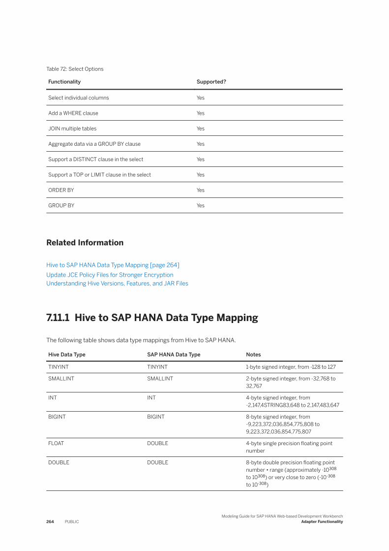
Table 72: Select Options
Functionality Supported?
Select individual columns Yes
Add a WHERE clause Yes
JOIN multiple tables Yes
Aggregate data via a GROUP BY clause Yes
Support a DISTINCT clause in the select Yes
Support a TOP or LIMIT clause in the select Yes
ORDER BY Yes
GROUP BY Yes
Related Information
Hive to SAP HANA Data Type Mapping [page 264]Update JCE Policy Files for Stronger EncryptionUnderstanding Hive Versions, Features, and JAR Files
7.11.1 Hive to SAP HANA Data Type Mapping
The following table shows data type mappings from Hive to SAP HANA.
Hive Data Type SAP HANA Data Type Notes
TINYINT TINYINT 1-byte signed integer, from -128 to 127
SMALLINT SMALLINT 2-byte signed integer, from -32,768 to 32,767
INT INT 4-byte signed integer, from -2,147,4STRING83,648 to 2,147,483,647
BIGINT BIGINT 8-byte signed integer, from -9,223,372,036,854,775,808 to 9,223,372,036,854,775,807
FLOAT DOUBLE 4-byte single precision floating point number
DOUBLE DOUBLE 8-byte double precision floating point number • range (approximately -10308
to 10308) or very close to zero (-10-308
to 10-308)
264 PUBLICModeling Guide for SAP HANA Web-based Development Workbench
Adapter Functionality
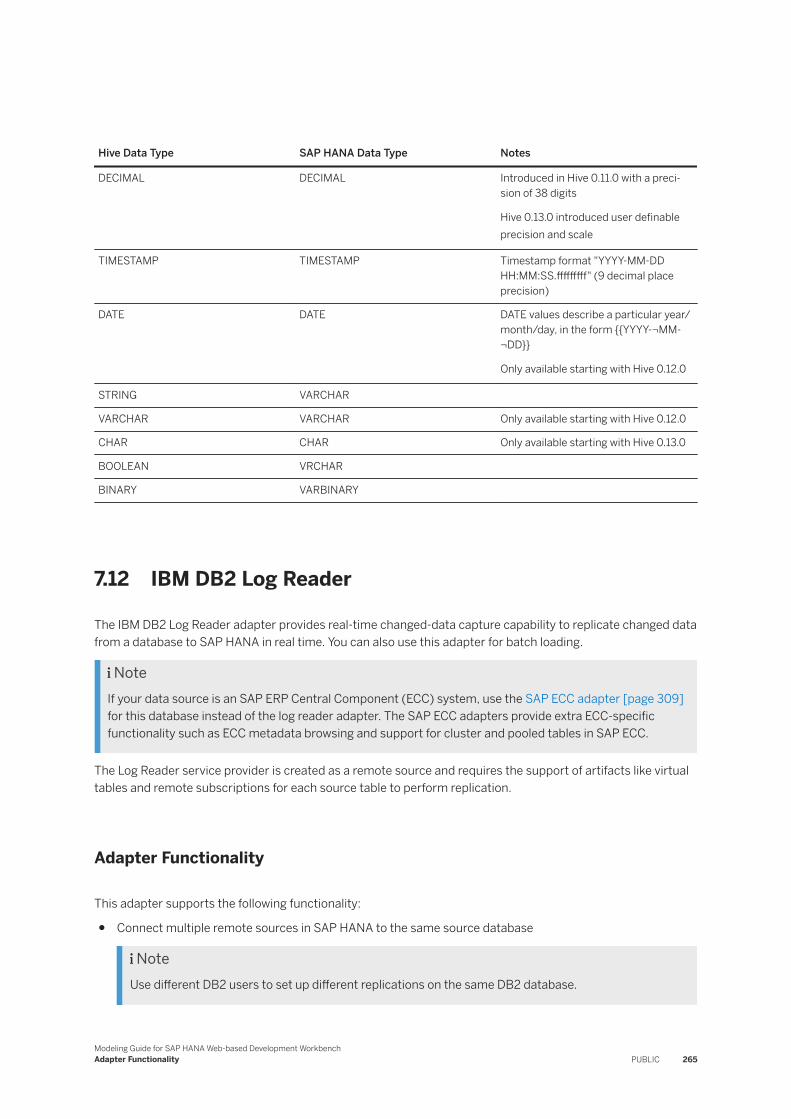
Hive Data Type SAP HANA Data Type Notes
DECIMAL DECIMAL Introduced in Hive 0.11.0 with a precision of 38 digits
Hive 0.13.0 introduced user definable precision and scale
TIMESTAMP TIMESTAMP Timestamp format "YYYY-MM-DD HH:MM:SS.fffffffff" (9 decimal place precision)
DATE DATE DATE values describe a particular year/month/day, in the form {{YYYY-¬MM-¬DD}}
Only available starting with Hive 0.12.0
STRING VARCHAR
VARCHAR VARCHAR Only available starting with Hive 0.12.0
CHAR CHAR Only available starting with Hive 0.13.0
BOOLEAN VRCHAR
BINARY VARBINARY
7.12 IBM DB2 Log Reader
The IBM DB2 Log Reader adapter provides real-time changed-data capture capability to replicate changed data from a database to SAP HANA in real time. You can also use this adapter for batch loading.
NoteIf your data source is an SAP ERP Central Component (ECC) system, use the SAP ECC adapter [page 309] for this database instead of the log reader adapter. The SAP ECC adapters provide extra ECC-specific functionality such as ECC metadata browsing and support for cluster and pooled tables in SAP ECC.
The Log Reader service provider is created as a remote source and requires the support of artifacts like virtual tables and remote subscriptions for each source table to perform replication.
Adapter Functionality
This adapter supports the following functionality:
● Connect multiple remote sources in SAP HANA to the same source database
NoteUse different DB2 users to set up different replications on the same DB2 database.
Modeling Guide for SAP HANA Web-based Development WorkbenchAdapter Functionality PUBLIC 265
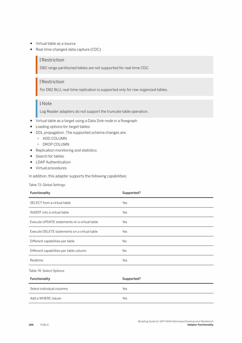
● Virtual table as a source● Real-time changed-data capture (CDC)
RestrictionDB2 range partitioned tables are not supported for real-time CDC.
RestrictionFor DB2 BLU, real-time replication is supported only for row-organized tables.
NoteLog Reader adapters do not support the truncate table operation.
● Virtual table as a target using a Data Sink node in a flowgraph● Loading options for target tables● DDL propagation. The supported schema changes are:
○ ADD COLUMN○ DROP COLUMN
● Replication monitoring and statistics● Search for tables● LDAP Authentication● Virtual procedures
In addition, this adapter supports the following capabilities:
Table 73: Global Settings
Functionality Supported?
SELECT from a virtual table Yes
INSERT into a virtual table Yes
Execute UPDATE statements on a virtual table Yes
Execute DELETE statements on a virtual table Yes
Different capabilities per table No
Different capabilities per table column No
Realtime Yes
Table 74: Select Options
Functionality Supported?
Select individual columns Yes
Add a WHERE clause Yes
266 PUBLICModeling Guide for SAP HANA Web-based Development Workbench
Adapter Functionality
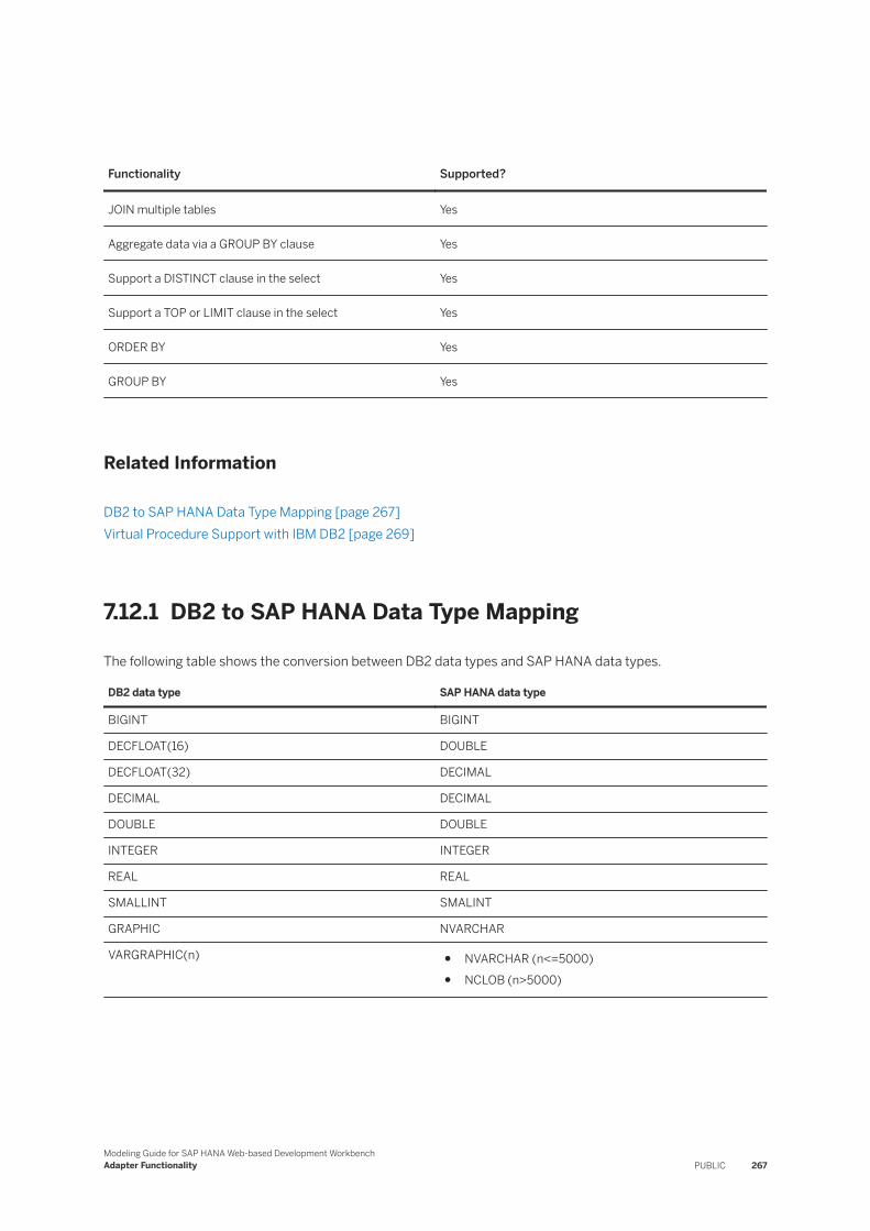
Functionality Supported?
JOIN multiple tables Yes
Aggregate data via a GROUP BY clause Yes
Support a DISTINCT clause in the select Yes
Support a TOP or LIMIT clause in the select Yes
ORDER BY Yes
GROUP BY Yes
Related Information
DB2 to SAP HANA Data Type Mapping [page 267]Virtual Procedure Support with IBM DB2 [page 269]
7.12.1 DB2 to SAP HANA Data Type Mapping
The following table shows the conversion between DB2 data types and SAP HANA data types.
DB2 data type SAP HANA data type
BIGINT BIGINT
DECFLOAT(16) DOUBLE
DECFLOAT(32) DECIMAL
DECIMAL DECIMAL
DOUBLE DOUBLE
INTEGER INTEGER
REAL REAL
SMALLINT SMALINT
GRAPHIC NVARCHAR
VARGRAPHIC(n) ● NVARCHAR (n<=5000)● NCLOB (n>5000)
Modeling Guide for SAP HANA Web-based Development WorkbenchAdapter Functionality PUBLIC 267

DB2 data type SAP HANA data type
NoteWhen the source table contains a VARGRAPHIC(n) column, the tablespace pagesize on this table should be set to 32k.
LONGVARGRAPHIC NCLOB
CHAR VARCHAR
CHARACTER VARCHAR
VARCHAR(n) ● VARCHAR (n<=5000)● CLOB (n>5000)
NoteWhen the source table contains a VARCHAR(n) column ,the tablespace pagesize on this table should be set to 32k.
LONG VARCHAR CLOB
CHAR FOR BIT DATA VARBINARY
VARCHAR(n) FOR BIT DATA VARBINARY(n)
NoteWhen the source table contains a VARCHAR(n) FOR BIT DATA column, the tablespace pagesize on this table should be set to 32k.
LONG VARCHAR FOR BIT DATA BLOB
DATE DATE
TIME TIME
TIMESTAMP TIMESTAMP
BLOB BLOB
CLOB CLOB
DBCLOB NCLOB
ROWID Unsupported
XML Unsupported
User-defined data types Unsupported
268 PUBLICModeling Guide for SAP HANA Web-based Development Workbench
Adapter Functionality
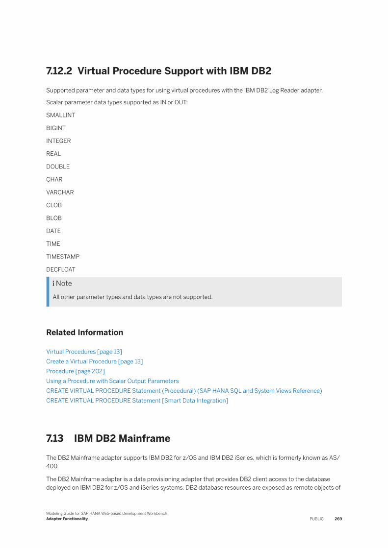
7.12.2 Virtual Procedure Support with IBM DB2Supported parameter and data types for using virtual procedures with the IBM DB2 Log Reader adapter.
Scalar parameter data types supported as IN or OUT:
SMALLINT
BIGINT
INTEGER
REAL
DOUBLE
CHAR
VARCHAR
CLOB
BLOB
DATE
TIME
TIMESTAMP
DECFLOAT
NoteAll other parameter types and data types are not supported.
Related Information
Virtual Procedures [page 13]Create a Virtual Procedure [page 13]Procedure [page 202]Using a Procedure with Scalar Output ParametersCREATE VIRTUAL PROCEDURE Statement (Procedural) (SAP HANA SQL and System Views Reference)CREATE VIRTUAL PROCEDURE Statement [Smart Data Integration]
7.13 IBM DB2 MainframeThe DB2 Mainframe adapter supports IBM DB2 for z/OS and IBM DB2 iSeries, which is formerly known as AS/400.
The DB2 Mainframe adapter is a data provisioning adapter that provides DB2 client access to the database deployed on IBM DB2 for z/OS and iSeries systems. DB2 database resources are exposed as remote objects of
Modeling Guide for SAP HANA Web-based Development WorkbenchAdapter Functionality PUBLIC 269
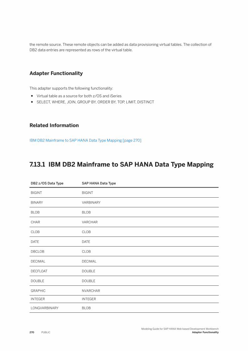
the remote source. These remote objects can be added as data provisioning virtual tables. The collection of DB2 data entries are represented as rows of the virtual table.
Adapter Functionality
This adapter supports the following functionality:
● Virtual table as a source for both z/OS and iSeries● SELECT, WHERE, JOIN, GROUP BY, ORDER BY, TOP, LIMIT, DISTINCT
Related Information
IBM DB2 Mainframe to SAP HANA Data Type Mapping [page 270]
7.13.1 IBM DB2 Mainframe to SAP HANA Data Type Mapping
DB2 z/OS Data Type SAP HANA Data Type
BIGINT BIGINT
BINARY VARBINARY
BLOB BLOB
CHAR VARCHAR
CLOB CLOB
DATE DATE
DBCLOB CLOB
DECIMAL DECIMAL
DECFLOAT DOUBLE
DOUBLE DOUBLE
GRAPHIC NVARCHAR
INTEGER INTEGER
LONGVARBINARY BLOB
270 PUBLICModeling Guide for SAP HANA Web-based Development Workbench
Adapter Functionality

DB2 z/OS Data Type SAP HANA Data Type
LONGVARCHAR CLOB
LONGVARGRAPHIC NCLOB
NCLOB NCLOB
REAL REAL
ROWID INTEGER
SMALLINT SMALLINT
TIME TIME
TIMESTAMP TIMESTAMP
VARBINARY VARBINARY
VARCHAR VARCHAR
VARGRAPHIC NVARCHAR
7.14 Microsoft Excel
This adapter lets SAP HANA users access Microsoft Excel files.
Adapter Functionality
This adapter supports the following functionality:
● Virtual table as a source● Search for tables● SharePoint as a source● SharePoint on Office365● SELECT from a virtual table
Related Information
MS Excel to SAP HANA Data Type Mapping [page 272]Reading Multiple Excel Files or Sheets [page 273]
Modeling Guide for SAP HANA Web-based Development WorkbenchAdapter Functionality PUBLIC 271
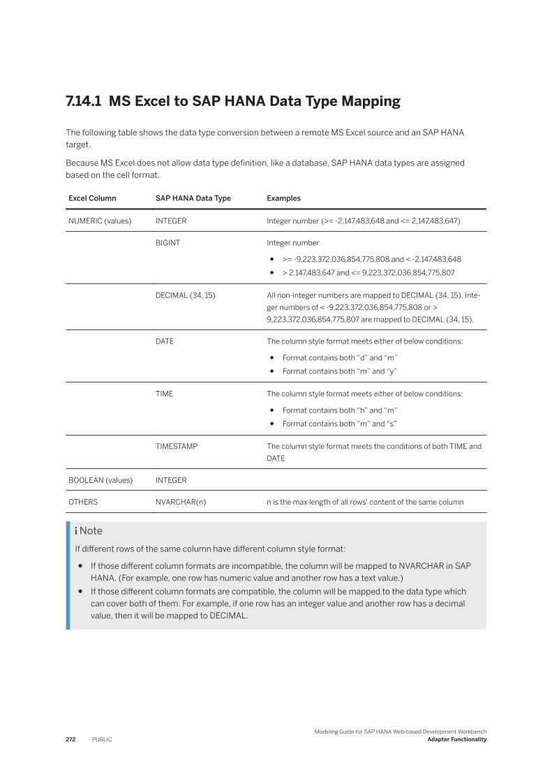
7.14.1 MS Excel to SAP HANA Data Type Mapping
The following table shows the data type conversion between a remote MS Excel source and an SAP HANA target.
Because MS Excel does not allow data type definition, like a database, SAP HANA data types are assigned based on the cell format.
Excel Column SAP HANA Data Type Examples
NUMERIC (values) INTEGER Integer number (>= -2,147,483,648 and <= 2,147,483,647)
BIGINT Integer number
● >= -9,223,372,036,854,775,808 and < -2,147,483,648● > 2,147,483,647 and <= 9,223,372,036,854,775,807
DECIMAL (34, 15) All non-integer numbers are mapped to DECIMAL (34, 15). Integer numbers of < -9,223,372,036,854,775,808 or > 9,223,372,036,854,775,807 are mapped to DECIMAL (34, 15).
DATE The column style format meets either of below conditions:
● Format contains both “d” and “m”● Format contains both “m” and “y”
TIME The column style format meets either of below conditions:
● Format contains both “h” and “m”● Format contains both “m” and “s”
TIMESTAMP The column style format meets the conditions of both TIME and DATE
BOOLEAN (values) INTEGER
OTHERS NVARCHAR(n) n is the max length of all rows' content of the same column
NoteIf different rows of the same column have different column style format:
● If those different column formats are incompatible, the column will be mapped to NVARCHAR in SAP HANA. (For example, one row has numeric value and another row has a text value.)
● If those different column formats are compatible, the column will be mapped to the data type which can cover both of them. For example, if one row has an integer value and another row has a decimal value, then it will be mapped to DECIMAL.
272 PUBLICModeling Guide for SAP HANA Web-based Development Workbench
Adapter Functionality

7.14.2 Reading Multiple Excel Files or Sheets
You can read multiple Excel files or sheets, or even a combination of both, using the Excel adapter.
If you have data that exists in multiple Excel files or sheets, you can use SQL to create a virtual table (SQL is the only means to do this). Before creating your virtual tables, make sure that your files and sheets have met the following requirements:
● All Excel files and sheets must have the same format.● The name of your Excel files or sheets must have same prefix.
You can get those files or sheets data by selecting the virtual table:
SELECT * FROM "SYSTEM"."VT_MYTABLE_XLSX";
NoteIf the path of those multiple Excel files is, for example, C:\usr\sap\dataprovagent\excel\demo\folders_xlsx, but the value of the Folder remote source configuration parameter is “demo”, you must provide a complete file path when creating virtual tables, otherwise the Excel adapter will throw an exception such as "SAP DBTech JDBC: [476]: invalid remote object name: Can't match any file whose name is like 'test*.xlsx'!". For example:
CREATE VIRTUAL TABLE "SYSTEM"."VT_MYTABLE_XLSX" at "ExcelSource"."<NULL>"."<NULL>"."folders_xlsx/test*.xlsx/abc_*";
Read multiple Excel files
CREATE VIRTUAL TABLE "SYSTEM"."VT_MYTABLE_XLSX" at "ExcelSource"."<NULL>"."<NULL>"."test*.xlsx/abc_sheet";
Read multiple Excel sheets
CREATE VIRTUAL TABLE "SYSTEM"."VT_MYTABLE_XLSX" at "ExcelSource"."<NULL>"."<NULL>"."test(1).xlsx/abc_*";
Read multiple Excel files and sheets
CREATE VIRTUAL TABLE "SYSTEM"."VT_MYTABLE_XLSX" at "ExcelSource"."<NULL>"."<NULL>"."test*.xlsx/abc_*";
Modeling Guide for SAP HANA Web-based Development WorkbenchAdapter Functionality PUBLIC 273

7.15 Microsoft Outlook
Access Microsoft Outlook data by using the Outlook adapter.
You can access Microsoft Outlook data stored in a PST file using the Outlook adapter.
This adapter supports the following functionality:
● Virtual table as a source
Related Information
PST File Tables [page 274]
7.15.1 PST File Tables
You can access the mail message and mail attachment tables.
The only tables that the adapter can access are the mail message table and the mail attachment table.
Mail Message Table
This table will store all the mail messages in this folder. Mails in sub-folders will not be replicated.
Column Name Data Type
MSG_ID VARCHAR(256)
SUBJECT NVARCHAR(4096)
SENDER_NAME NVARCHAR(4096)
CREATION_TIME TIMESTAMP
LAST_MDF_TIME TIMESTAMP
COMMENT NCLOB
DESC_NODE_ID VARCHAR(1024)
SENDER_MAIL_ADDR VARCHAR(256)
RECIPIENTS CLOB
274 PUBLICModeling Guide for SAP HANA Web-based Development Workbench
Adapter Functionality
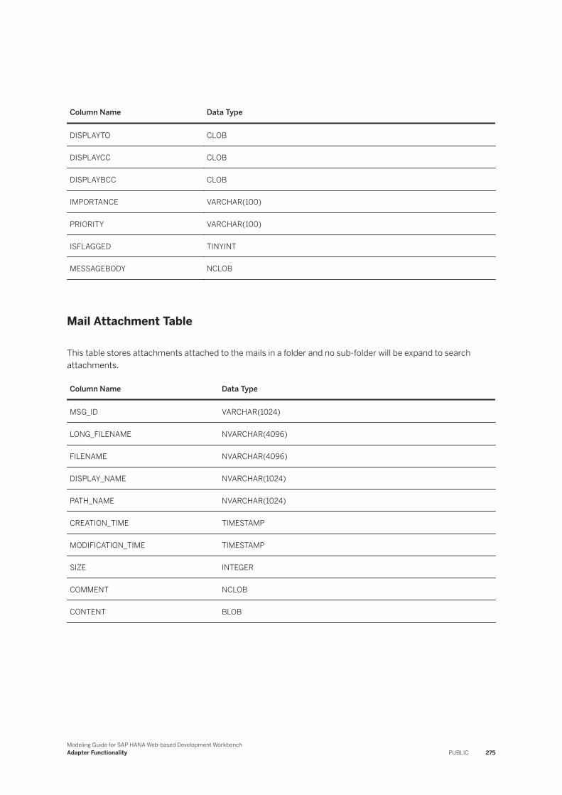
Column Name Data Type
DISPLAYTO CLOB
DISPLAYCC CLOB
DISPLAYBCC CLOB
IMPORTANCE VARCHAR(100)
PRIORITY VARCHAR(100)
ISFLAGGED TINYINT
MESSAGEBODY NCLOB
Mail Attachment Table
This table stores attachments attached to the mails in a folder and no sub-folder will be expand to search attachments.
Column Name Data Type
MSG_ID VARCHAR(1024)
LONG_FILENAME NVARCHAR(4096)
FILENAME NVARCHAR(4096)
DISPLAY_NAME NVARCHAR(1024)
PATH_NAME NVARCHAR(1024)
CREATION_TIME TIMESTAMP
MODIFICATION_TIME TIMESTAMP
SIZE INTEGER
COMMENT NCLOB
CONTENT BLOB
Modeling Guide for SAP HANA Web-based Development WorkbenchAdapter Functionality PUBLIC 275
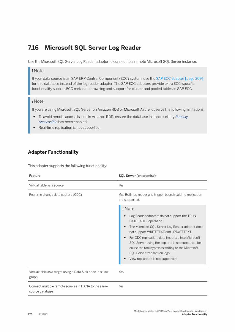
7.16 Microsoft SQL Server Log Reader
Use the Microsoft SQL Server Log Reader adapter to connect to a remote Microsoft SQL Server instance.
NoteIf your data source is an SAP ERP Central Component (ECC) system, use the SAP ECC adapter [page 309] for this database instead of the log reader adapter. The SAP ECC adapters provide extra ECC-specific functionality such as ECC metadata browsing and support for cluster and pooled tables in SAP ECC.
NoteIf you are using Microsoft SQL Server on Amazon RDS or Microsoft Azure, observe the following limitations:
● To avoid remote access issues in Amazon RDS, ensure the database instance setting Publicly Acccessible has been enabled.
● Real-time replication is not supported.
Adapter Functionality
This adapter supports the following functionality:
Feature SQL Server (on premise)
Virtual table as a source Yes
Realtime change data capture (CDC) Yes. Both log reader and trigger-based realtime replication are supported.
Note● Log Reader adapters do not support the TRUN
CATE TABLE operation.● The Microsoft SQL Server Log Reader adapter does
not support WRITETEXT and UPDATETEXT.● For CDC replication, data imported into Microsoft
SQL Server using the bcp tool is not supported because the tool bypasses writing to the Microsoft SQL Server transaction logs.
● View replication is not supported.
Virtual table as a target using a Data Sink node in a flow-graph
Yes
Connect multiple remote sources in HANA to the same source database
Yes
276 PUBLICModeling Guide for SAP HANA Web-based Development Workbench
Adapter Functionality
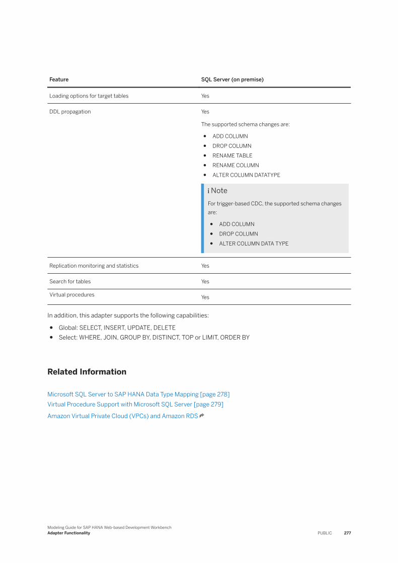
Feature SQL Server (on premise)
Loading options for target tables Yes
DDL propagation Yes
The supported schema changes are:
● ADD COLUMN● DROP COLUMN● RENAME TABLE● RENAME COLUMN● ALTER COLUMN DATATYPE
NoteFor trigger-based CDC, the supported schema changes are:
● ADD COLUMN● DROP COLUMN● ALTER COLUMN DATA TYPE
Replication monitoring and statistics Yes
Search for tables Yes
Virtual procedures Yes
In addition, this adapter supports the following capabilities:
● Global: SELECT, INSERT, UPDATE, DELETE● Select: WHERE, JOIN, GROUP BY, DISTINCT, TOP or LIMIT, ORDER BY
Related Information
Microsoft SQL Server to SAP HANA Data Type Mapping [page 278]Virtual Procedure Support with Microsoft SQL Server [page 279]
Amazon Virtual Private Cloud (VPCs) and Amazon RDS
Modeling Guide for SAP HANA Web-based Development WorkbenchAdapter Functionality PUBLIC 277
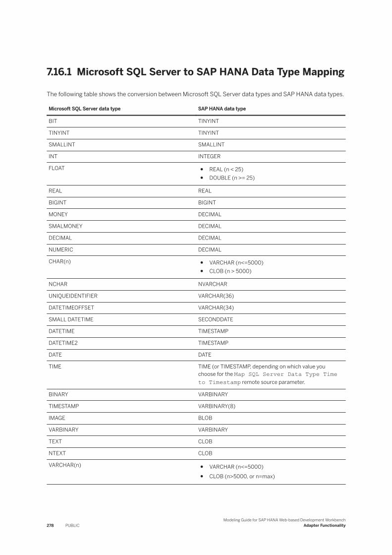
7.16.1 Microsoft SQL Server to SAP HANA Data Type Mapping
The following table shows the conversion between Microsoft SQL Server data types and SAP HANA data types.
Microsoft SQL Server data type SAP HANA data type
BIT TINYINT
TINYINT TINYINT
SMALLINT SMALLINT
INT INTEGER
FLOAT ● REAL (n < 25)● DOUBLE (n >= 25)
REAL REAL
BIGINT BIGINT
MONEY DECIMAL
SMALMONEY DECIMAL
DECIMAL DECIMAL
NUMERIC DECIMAL
CHAR(n) ● VARCHAR (n<=5000)● CLOB (n > 5000)
NCHAR NVARCHAR
UNIQUEIDENTIFIER VARCHAR(36)
DATETIMEOFFSET VARCHAR(34)
SMALL DATETIME SECONDDATE
DATETIME TIMESTAMP
DATETIME2 TIMESTAMP
DATE DATE
TIME TIME (or TIMESTAMP, depending on which value you choose for the Map SQL Server Data Type Time to Timestamp remote source parameter.
BINARY VARBINARY
TIMESTAMP VARBINARY(8)
IMAGE BLOB
VARBINARY VARBINARY
TEXT CLOB
NTEXT CLOB
VARCHAR(n) ● VARCHAR (n<=5000)● CLOB (n>5000, or n=max)
278 PUBLICModeling Guide for SAP HANA Web-based Development Workbench
Adapter Functionality
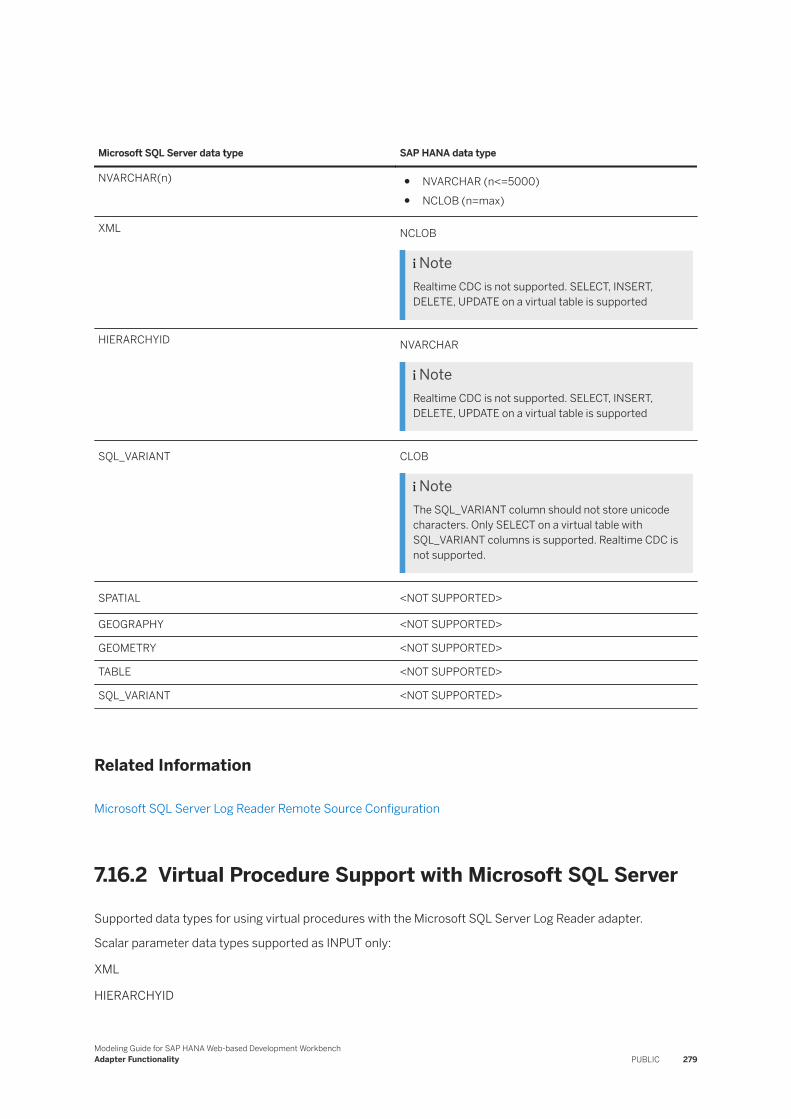
Microsoft SQL Server data type SAP HANA data type
NVARCHAR(n) ● NVARCHAR (n<=5000)● NCLOB (n=max)
XML NCLOB
NoteRealtime CDC is not supported. SELECT, INSERT, DELETE, UPDATE on a virtual table is supported
HIERARCHYID NVARCHAR
NoteRealtime CDC is not supported. SELECT, INSERT, DELETE, UPDATE on a virtual table is supported
SQL_VARIANT CLOB
NoteThe SQL_VARIANT column should not store unicode characters. Only SELECT on a virtual table with SQL_VARIANT columns is supported. Realtime CDC is not supported.
SPATIAL <NOT SUPPORTED>
GEOGRAPHY <NOT SUPPORTED>
GEOMETRY <NOT SUPPORTED>
TABLE <NOT SUPPORTED>
SQL_VARIANT <NOT SUPPORTED>
Related Information
Microsoft SQL Server Log Reader Remote Source Configuration
7.16.2 Virtual Procedure Support with Microsoft SQL Server
Supported data types for using virtual procedures with the Microsoft SQL Server Log Reader adapter.
Scalar parameter data types supported as INPUT only:
XML
HIERARCHYID
Modeling Guide for SAP HANA Web-based Development WorkbenchAdapter Functionality PUBLIC 279
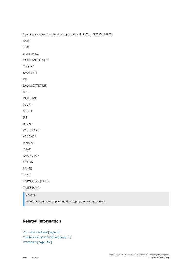
Scalar parameter data types supported as INPUT or OUT/OUTPUT:
DATE
TIME
DATETIME2
DATETIMEOFFSET
TINYINT
SMALLINT
INT
SMALLDATETIME
REAL
DATETIME
FLOAT
NTEXT
BIT
BIGINT
VARBINARY
VARCHAR
BINARY
CHAR
NVARCHAR
NCHAR
IMAGE
TEXT
UNIQUEIDENTIFIER
TIMESTAMP
NoteAll other parameter types and data types are not supported.
Related Information
Virtual Procedures [page 13]Create a Virtual Procedure [page 13]Procedure [page 202]
280 PUBLICModeling Guide for SAP HANA Web-based Development Workbench
Adapter Functionality
Using a Procedure with Scalar Output ParametersCREATE VIRTUAL PROCEDURE Statement (Procedural) (SAP HANA SQL and System Views Reference)CREATE VIRTUAL PROCEDURE Statement [Smart Data Integration]
7.17 OData
Set up access to the OData service provider and its data and metadata.
Open Data Protocol (OData) is a standardized protocol for exposing and accessing information from various sources, based on core protocols including HTTP, AtomPub (Atom Publishing Protocol), XML, and JSON (Java Script Object Notation). OData provides a standard API on service data and metadata presentation, and data operations.
The SAP OData adapter provides OData client access to the OData service provider and its data and metadata. The OData service provider is created as a remote source. OData resources are exposed as metadata tables of the remote source. These metadata tables can be added as virtual tables. An SAP HANA SQL query can then access the OData data. Collections of OData data entries are represented as rows of the virtual table.
The OData adapter supports the following functionality:
● Virtual table as a source● Virtual table as a target using a Data Sink in a flowgraph
The data of the main navigation entities can be accessed via SQL with the following restrictions:
● Without a join, selected projection columns appear in the OData system query “$select”.● With a join, columns of the joined table, which is the associated OData entity, can occur in the projection.
Selected projection columns appear in the OData system query “$select”. All joined tables appear in the OData system query “$expand”.
● Due to a restriction of the OData system queries “$select” and “$orderby”, no expressions can occur in the Projection and the Order By clause.
● The Where clause supports logical, arithmetic, and ISNULL operators, string functions, and date functions. The expression is translated into the OData system query “$filter”.
Refer to OData documentation for the OData URI conventions.
Related Information
OData to SAP HANA Data Type Mapping [page 282]Retrieve SAP SuccessFactors Historical Data [page 283]Enabling Pagination in SuccessFactors [page 284]Connecting to SAP SuccessFactors with OAuth 2.0 Authentication [page 284]
URI Conventions
Modeling Guide for SAP HANA Web-based Development WorkbenchAdapter Functionality PUBLIC 281
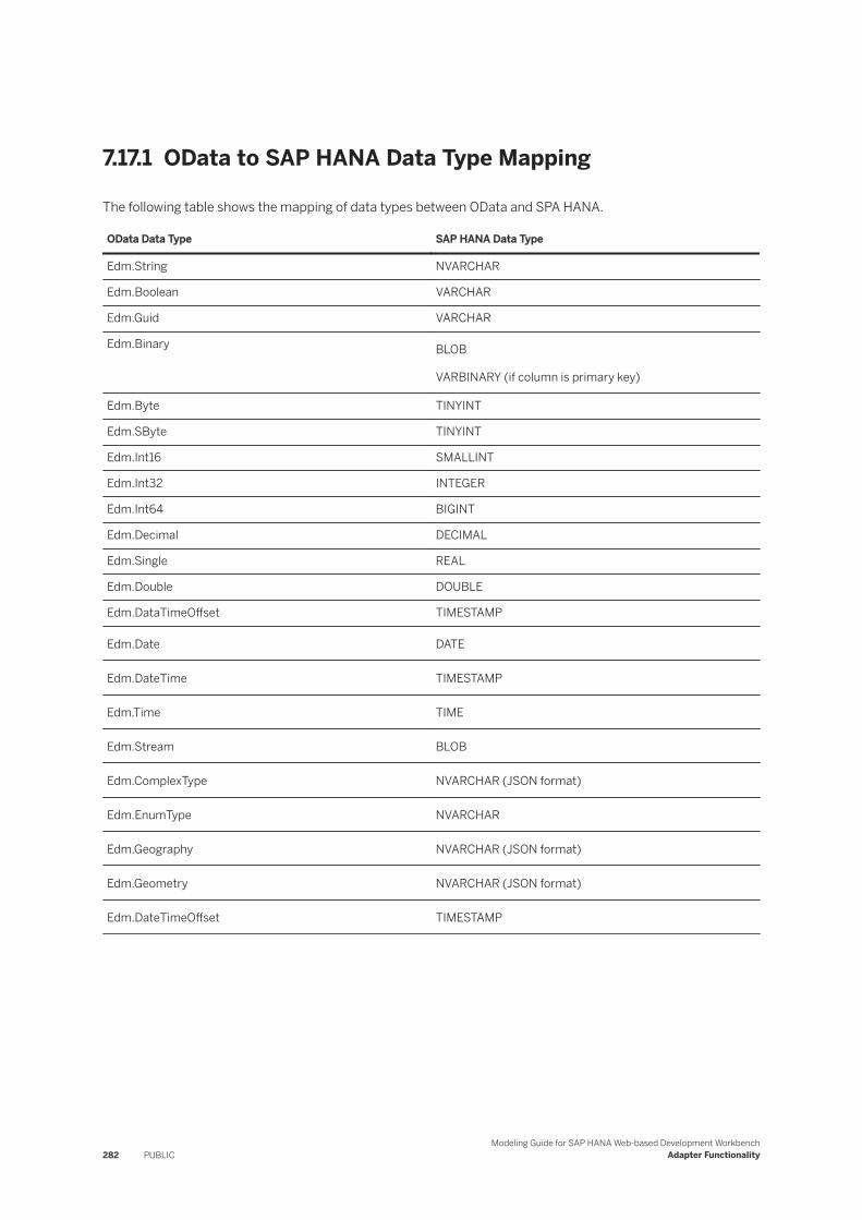
7.17.1 OData to SAP HANA Data Type Mapping
The following table shows the mapping of data types between OData and SPA HANA.
OData Data Type SAP HANA Data Type
Edm.String NVARCHAR
Edm.Boolean VARCHAR
Edm.Guid VARCHAR
Edm.Binary BLOB
VARBINARY (if column is primary key)
Edm.Byte TINYINT
Edm.SByte TINYINT
Edm.Int16 SMALLINT
Edm.Int32 INTEGER
Edm.Int64 BIGINT
Edm.Decimal DECIMAL
Edm.Single REAL
Edm.Double DOUBLE
Edm.DataTimeOffset TIMESTAMP
Edm.Date DATE
Edm.DateTime TIMESTAMP
Edm.Time TIME
Edm.Stream BLOB
Edm.ComplexType NVARCHAR (JSON format)
Edm.EnumType NVARCHAR
Edm.Geography NVARCHAR (JSON format)
Edm.Geometry NVARCHAR (JSON format)
Edm.DateTimeOffset TIMESTAMP
282 PUBLICModeling Guide for SAP HANA Web-based Development Workbench
Adapter Functionality

7.17.2 Retrieve SAP SuccessFactors Historical Data
You can use SAP SuccessFactors fromDate/toDate/asOfDate keywords to retrieve historical data (effective-dated entities), using the OData adapter.
Context
You can use data provisioning parameters when creating a virtual table to configure fromDate/toDate/asOfDate values.
NoteYou need to refresh the OData adapter after upgrading to access these capabilities. Also, if you have existing virtual tables accessed by the OData adapter, you must drop and recreate the tables to gain access the data provisioning parameters.
Procedure
1. Use the following query to check whether the data provisioning properties exist in the created virtual table: SELECT PROPERTY, VALUE FROM PUBLIC.VIRTUAL_TABLE_PROPERTIES WHERE SCHEMA_NAME = '<virtual table schema>' AND TABLE_NAME = '<virtual table name>'
2. If the data provisioning properties exist, use data provisioning parameters in your SELECT query.
For example:
SELECT * FROM "SYSTEM"."odata_sfsf_EmpJob" WHERE "userId" = 'spappar1' WITH DATAPROVISIONING PARAMETERS('<PropertyGroup name="__DP_READER_OPTIONS__"><PropertyGroup displayName="EmpJob" id="0" isRepeatable="false" name="EmpJob"><PropertyEntry name="asOfDate"></PropertyEntry><PropertyEntry name="fromDate">2010-01-01</PropertyEntry><PropertyEntry name="toDate"></PropertyEntry></PropertyGroup></PropertyGroup>')
Results
The underlying OData HTTP request will now have extra fromDate/toDate/asOfDate keyword(s) to extract SAP SuccessFactors historical data.
Modeling Guide for SAP HANA Web-based Development WorkbenchAdapter Functionality PUBLIC 283

Related Information
Querying Effective-Dated EntitiesHow can I query effective dated queries?
7.17.3 Enabling Pagination in SuccessFactors
You can use data provisioning parameters with the OData adapter to enable pagination when extracting data from SuccessFactors.
You can use the “paging” parameter in your SELECT statement.
SELECT * FROM "odata_sfsf_User" WITH DATAPROVISIONING PARAMETERS ('<PropertyGroup name="__DP_READER_OPTIONS__"><PropertyGroup displayName="User" id="0" isRepeatable="false" name="User"><PropertyEntry name="asOfDate"></PropertyEntry><PropertyEntry name="fromDate"></PropertyEntry><PropertyEntry name="toDate"></PropertyEntry><PropertyEntry name="paging">cursor</PropertyEntry></PropertyGroup> </PropertyGroup>');
The paging property value is appended to the HTTP request URL. For example:
https://apisalesdemo2.successfactors.eu/odata/v2/User?$select=businessPhone,city,country,department,division,email,empId,firstName,jobTitle,lastName,state,userId,username,zipCode&$format=json&paging=cursor
Related Information
SAP SuccessFactors HCM Suite OData API: Developer Guide - Server Pagination
7.17.4 Connecting to SAP SuccessFactors with OAuth 2.0 Authentication
When you are using SAP HANA Cloud, you can create an OData remote source that connects to an SAP SuccessFactors OData Endpoint using OAuth 2.0 authentication.
For example:
CREATE REMOTE SOURCE "odata_sfsfoauth2" ADAPTER "ODataAdapter" AT LOCATION DPSERVER CONFIGURATION '<?xml version="1.0" encoding="UTF-8" standalone="yes"?> <ConnectionProperties name="connection_properties"> <PropertyEntry name="URL"><MY_SFSF_INSTANCE>/odata/v2/</PropertyEntry> ... <PropertyEntry name="authenticationType">OAuth2Saml</PropertyEntry>
284 PUBLICModeling Guide for SAP HANA Web-based Development Workbench
Adapter Functionality
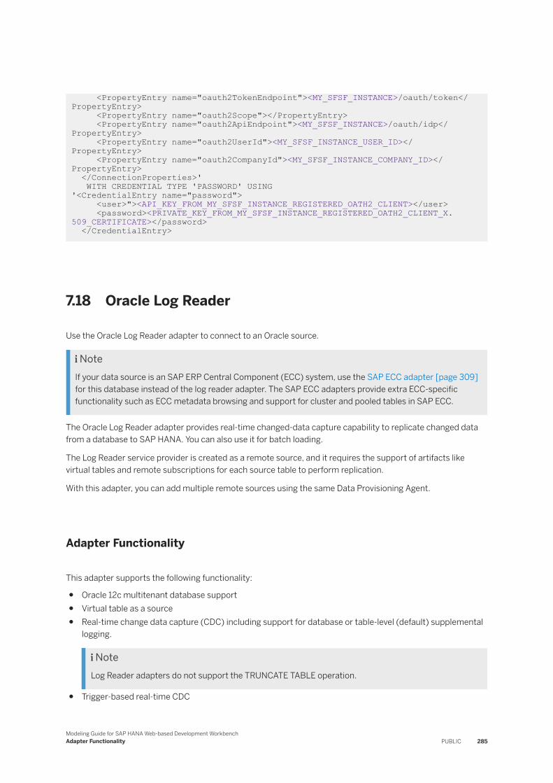
<PropertyEntry name="oauth2TokenEndpoint"><MY_SFSF_INSTANCE>/oauth/token</PropertyEntry> <PropertyEntry name="oauth2Scope"></PropertyEntry> <PropertyEntry name="oauth2ApiEndpoint"><MY_SFSF_INSTANCE>/oauth/idp</PropertyEntry> <PropertyEntry name="oauth2UserId"><MY_SFSF_INSTANCE_USER_ID></PropertyEntry> <PropertyEntry name="oauth2CompanyId"><MY_SFSF_INSTANCE_COMPANY_ID></PropertyEntry> </ConnectionProperties>' WITH CREDENTIAL TYPE 'PASSWORD' USING '<CredentialEntry name="password"> <user>"><API_KEY_FROM_MY_SFSF_INSTANCE_REGISTERED_OATH2_CLIENT></user> <password><PRIVATE_KEY_FROM_MY_SFSF_INSTANCE_REGISTERED_OATH2_CLIENT_X.509_CERTIFICATE></password> </CredentialEntry>
7.18 Oracle Log Reader
Use the Oracle Log Reader adapter to connect to an Oracle source.
NoteIf your data source is an SAP ERP Central Component (ECC) system, use the SAP ECC adapter [page 309] for this database instead of the log reader adapter. The SAP ECC adapters provide extra ECC-specific functionality such as ECC metadata browsing and support for cluster and pooled tables in SAP ECC.
The Oracle Log Reader adapter provides real-time changed-data capture capability to replicate changed data from a database to SAP HANA. You can also use it for batch loading.
The Log Reader service provider is created as a remote source, and it requires the support of artifacts like virtual tables and remote subscriptions for each source table to perform replication.
With this adapter, you can add multiple remote sources using the same Data Provisioning Agent.
Adapter Functionality
This adapter supports the following functionality:
● Oracle 12c multitenant database support● Virtual table as a source● Real-time change data capture (CDC) including support for database or table-level (default) supplemental
logging.
NoteLog Reader adapters do not support the TRUNCATE TABLE operation.
● Trigger-based real-time CDC
Modeling Guide for SAP HANA Web-based Development WorkbenchAdapter Functionality PUBLIC 285
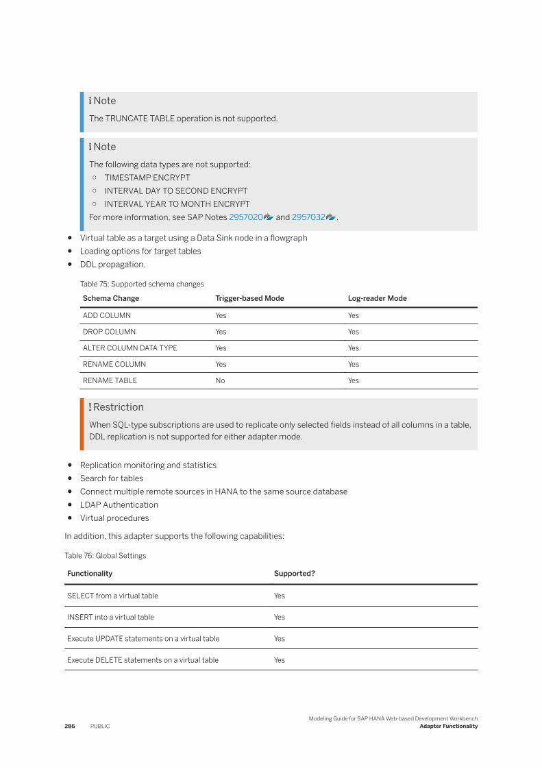
NoteThe TRUNCATE TABLE operation is not supported.
NoteThe following data types are not supported:○ TIMESTAMP ENCRYPT○ INTERVAL DAY TO SECOND ENCRYPT○ INTERVAL YEAR TO MONTH ENCRYPT
For more information, see SAP Notes 2957020 and 2957032 .
● Virtual table as a target using a Data Sink node in a flowgraph● Loading options for target tables● DDL propagation.
Table 75: Supported schema changes
Schema Change Trigger-based Mode Log-reader Mode
ADD COLUMN Yes Yes
DROP COLUMN Yes Yes
ALTER COLUMN DATA TYPE Yes Yes
RENAME COLUMN Yes Yes
RENAME TABLE No Yes
RestrictionWhen SQL-type subscriptions are used to replicate only selected fields instead of all columns in a table, DDL replication is not supported for either adapter mode.
● Replication monitoring and statistics● Search for tables● Connect multiple remote sources in HANA to the same source database● LDAP Authentication● Virtual procedures
In addition, this adapter supports the following capabilities:
Table 76: Global Settings
Functionality Supported?
SELECT from a virtual table Yes
INSERT into a virtual table Yes
Execute UPDATE statements on a virtual table Yes
Execute DELETE statements on a virtual table Yes
286 PUBLICModeling Guide for SAP HANA Web-based Development Workbench
Adapter Functionality
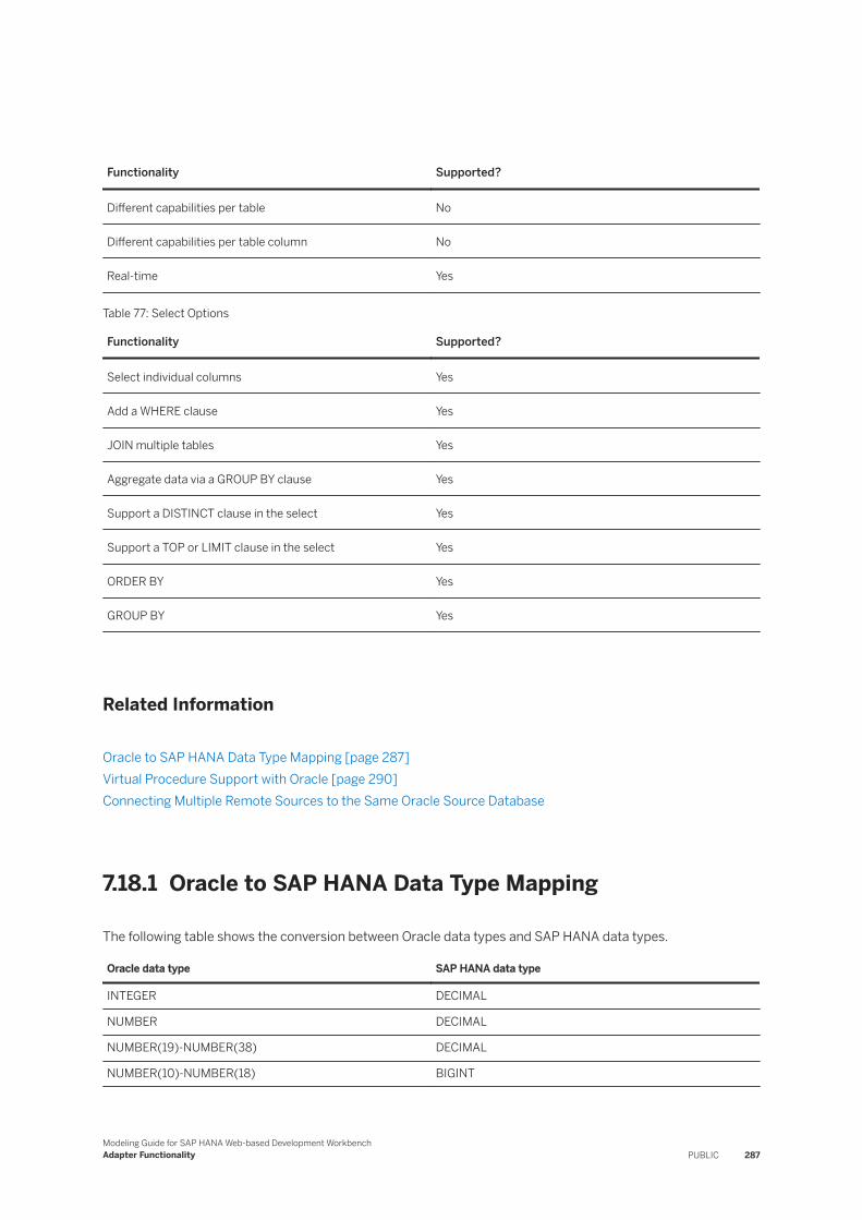
Functionality Supported?
Different capabilities per table No
Different capabilities per table column No
Real-time Yes
Table 77: Select Options
Functionality Supported?
Select individual columns Yes
Add a WHERE clause Yes
JOIN multiple tables Yes
Aggregate data via a GROUP BY clause Yes
Support a DISTINCT clause in the select Yes
Support a TOP or LIMIT clause in the select Yes
ORDER BY Yes
GROUP BY Yes
Related Information
Oracle to SAP HANA Data Type Mapping [page 287]Virtual Procedure Support with Oracle [page 290]Connecting Multiple Remote Sources to the Same Oracle Source Database
7.18.1 Oracle to SAP HANA Data Type Mapping
The following table shows the conversion between Oracle data types and SAP HANA data types.
Oracle data type SAP HANA data type
INTEGER DECIMAL
NUMBER DECIMAL
NUMBER(19)-NUMBER(38) DECIMAL
NUMBER(10)-NUMBER(18) BIGINT
Modeling Guide for SAP HANA Web-based Development WorkbenchAdapter Functionality PUBLIC 287

Oracle data type SAP HANA data type
NUMBER(5)-NUMBER(9) INTEGER
NUMBER(2)-NUMBER(4) SMALLINT
NUMBER(1) TINYINT
NUMBER(p,s) ● DOUBLE (if s > p)● DECIMAL (if 0 < s <= P)● SMALLINT (if s < 0 and p-s <= 4)● INTEGER (if s < 0 and 4 < p-s <= 9)● BIGINT (if s < 0 and 9 < p-s <= 18)● DECIMAL (if s< 0 and p-s > 18)
FLOAT DOUBLE
FLOAT(1)-FLOAT(24) REAL
FLOAT(25)-FLOAT(126) DOUBLE
BINARY_FLOAT REAL
BINARY_DOUBLE DOUBLE
DATE
Note“BC” dates are not supported.
TIMESTAMP
TIMESTAMP(n)
Note“BC” dates are not supported.
TIMESTAMP
CHAR VARCHAR
NCHAR NVARCHAR
VARCHAR2 VARCHAR
NVARCHAR2 NVARCHAR
BLOB BLOB
BFILE BLOB
RAW VARBINARY
LONG CLOB
LONG RAW BLOB
CLOB CLOB/NCLOB
NCLOB NCLOB
INTERVAL VARCHAR
TIMESTAMP WITH TIME ZONE VARCHAR
288 PUBLICModeling Guide for SAP HANA Web-based Development Workbench
Adapter Functionality
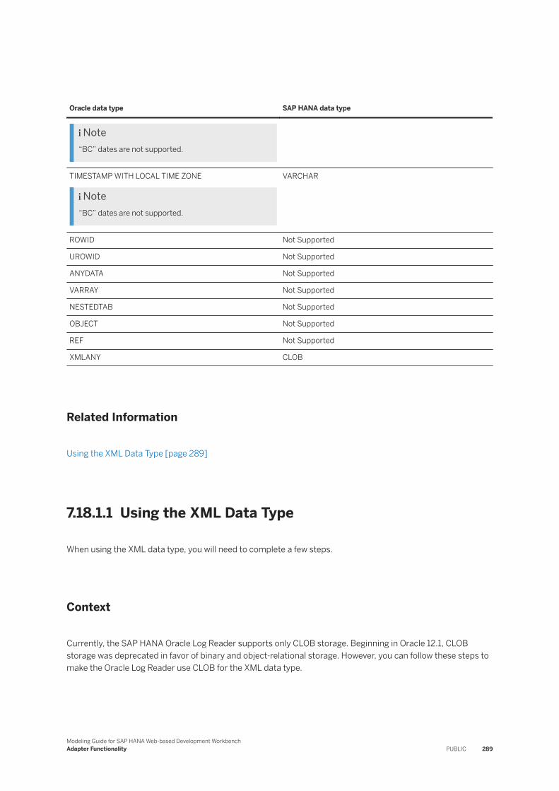
Oracle data type SAP HANA data type
Note“BC” dates are not supported.
TIMESTAMP WITH LOCAL TIME ZONE
Note“BC” dates are not supported.
VARCHAR
ROWID Not Supported
UROWID Not Supported
ANYDATA Not Supported
VARRAY Not Supported
NESTEDTAB Not Supported
OBJECT Not Supported
REF Not Supported
XMLANY CLOB
Related Information
Using the XML Data Type [page 289]
7.18.1.1 Using the XML Data Type
When using the XML data type, you will need to complete a few steps.
Context
Currently, the SAP HANA Oracle Log Reader supports only CLOB storage. Beginning in Oracle 12.1, CLOB storage was deprecated in favor of binary and object-relational storage. However, you can follow these steps to make the Oracle Log Reader use CLOB for the XML data type.
Modeling Guide for SAP HANA Web-based Development WorkbenchAdapter Functionality PUBLIC 289
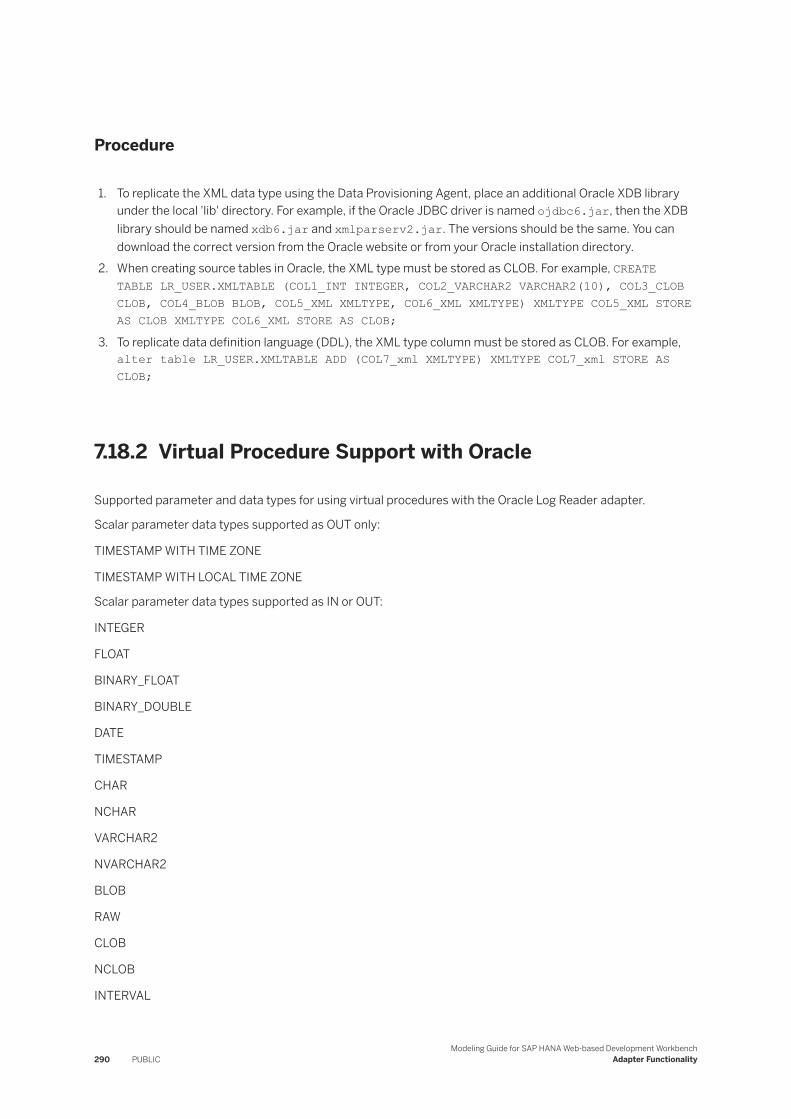
Procedure
1. To replicate the XML data type using the Data Provisioning Agent, place an additional Oracle XDB library under the local 'lib' directory. For example, if the Oracle JDBC driver is named ojdbc6.jar, then the XDB library should be named xdb6.jar and xmlparserv2.jar. The versions should be the same. You can download the correct version from the Oracle website or from your Oracle installation directory.
2. When creating source tables in Oracle, the XML type must be stored as CLOB. For example, CREATE TABLE LR_USER.XMLTABLE (COL1_INT INTEGER, COL2_VARCHAR2 VARCHAR2(10), COL3_CLOB CLOB, COL4_BLOB BLOB, COL5_XML XMLTYPE, COL6_XML XMLTYPE) XMLTYPE COL5_XML STORE AS CLOB XMLTYPE COL6_XML STORE AS CLOB;
3. To replicate data definition language (DDL), the XML type column must be stored as CLOB. For example, alter table LR_USER.XMLTABLE ADD (COL7_xml XMLTYPE) XMLTYPE COL7_xml STORE AS CLOB;
7.18.2 Virtual Procedure Support with Oracle
Supported parameter and data types for using virtual procedures with the Oracle Log Reader adapter.
Scalar parameter data types supported as OUT only:
TIMESTAMP WITH TIME ZONE
TIMESTAMP WITH LOCAL TIME ZONE
Scalar parameter data types supported as IN or OUT:
INTEGER
FLOAT
BINARY_FLOAT
BINARY_DOUBLE
DATE
TIMESTAMP
CHAR
NCHAR
VARCHAR2
NVARCHAR2
BLOB
RAW
CLOB
NCLOB
INTERVAL
290 PUBLICModeling Guide for SAP HANA Web-based Development Workbench
Adapter Functionality
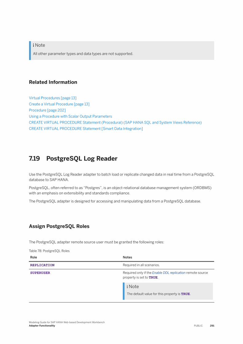
NoteAll other parameter types and data types are not supported.
Related Information
Virtual Procedures [page 13]Create a Virtual Procedure [page 13]Procedure [page 202]Using a Procedure with Scalar Output ParametersCREATE VIRTUAL PROCEDURE Statement (Procedural) (SAP HANA SQL and System Views Reference)CREATE VIRTUAL PROCEDURE Statement [Smart Data Integration]
7.19 PostgreSQL Log Reader
Use the PostgreSQL Log Reader adapter to batch load or replicate changed data in real time from a PostgreSQL database to SAP HANA.
PostgreSQL, often referred to as “Postgres”, is an object-relational database management system (ORDBMS) with an emphasis on extensibility and standards compliance.
The PostgreSQL adapter is designed for accessing and manipulating data from a PostgreSQL database.
Assign PostgreSQL Roles
The PostgreSQL adapter remote source user must be granted the following roles:
Table 78: PostgreSQL Roles
Role Notes
REPLICATION Required in all scenarios.
SUPERUSER Required only if the Enable DDL replication remote source property is set to TRUE.
NoteThe default value for this property is TRUE.
Modeling Guide for SAP HANA Web-based Development WorkbenchAdapter Functionality PUBLIC 291
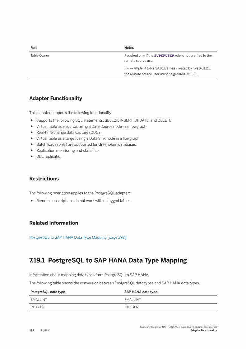
Role Notes
Table Owner Required only if the SUPERUSER role is not granted to the remote source user.
For example, if table TABLE1 was created by role ROLE1, the remote source user must be granted ROLE1.
Adapter Functionality
This adapter supports the following functionality:
● Supports the following SQL statements: SELECT, INSERT, UPDATE, and DELETE● Virtual table as a source, using a Data Source node in a flowgraph● Real-time change data capture (CDC)● Virtual table as a target using a Data Sink node in a flowgraph● Batch loads (only) are supported for Greenplum databases.● Replication monitoring and statistics● DDL replication
Restrictions
The following restriction applies to the PostgreSQL adapter:
● Remote subscriptions do not work with unlogged tables.
Related Information
PostgreSQL to SAP HANA Data Type Mapping [page 292]
7.19.1 PostgreSQL to SAP HANA Data Type Mapping
Information about mapping data types from PostgreSQL to SAP HANA.
The following table shows the conversion between PostgreSQL data types and SAP HANA data types.
PostgreSQL data type SAP HANA data type
SMALLINT SMALLINT
INTEGER INTEGER
292 PUBLICModeling Guide for SAP HANA Web-based Development Workbench
Adapter Functionality
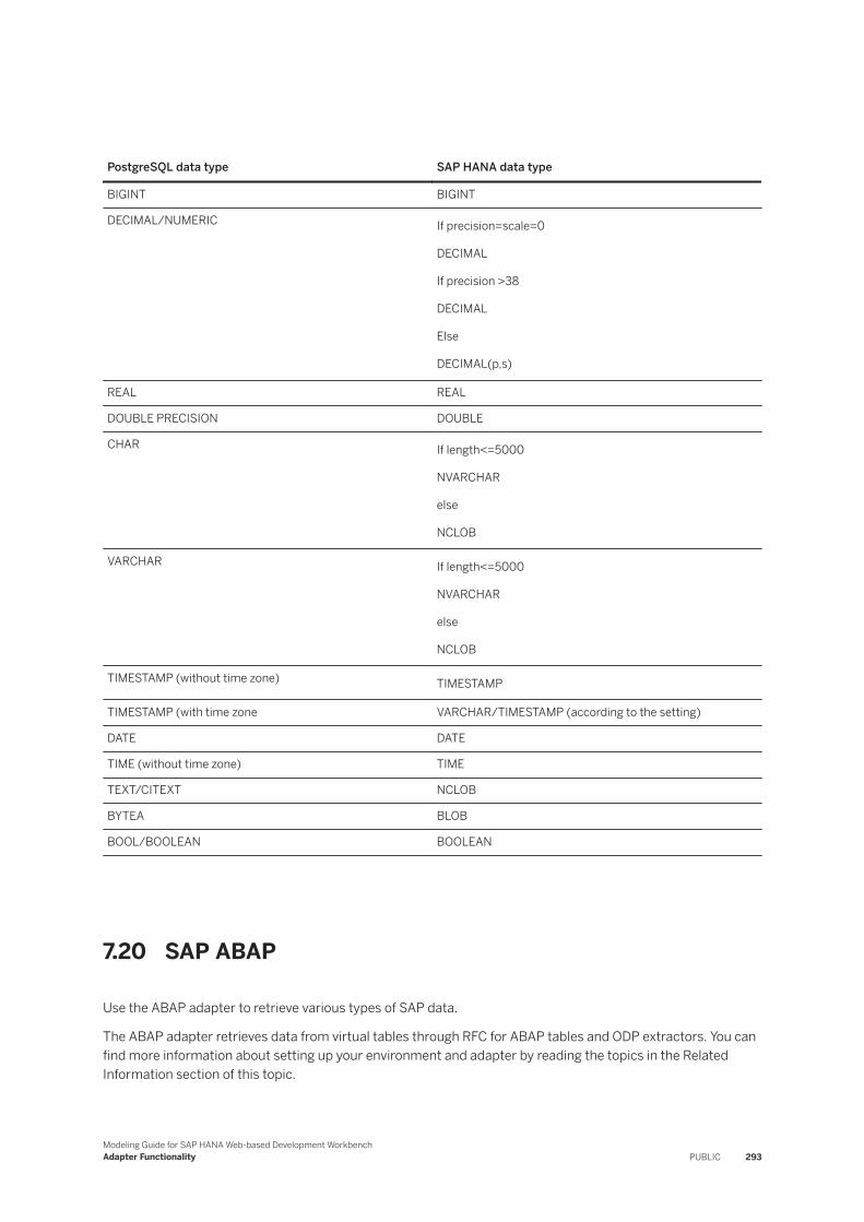
PostgreSQL data type SAP HANA data type
BIGINT BIGINT
DECIMAL/NUMERIC If precision=scale=0
DECIMAL
If precision >38
DECIMAL
Else
DECIMAL(p,s)
REAL REAL
DOUBLE PRECISION DOUBLE
CHAR If length<=5000
NVARCHAR
else
NCLOB
VARCHAR If length<=5000
NVARCHAR
else
NCLOB
TIMESTAMP (without time zone) TIMESTAMP
TIMESTAMP (with time zone VARCHAR/TIMESTAMP (according to the setting)
DATE DATE
TIME (without time zone) TIME
TEXT/CITEXT NCLOB
BYTEA BLOB
BOOL/BOOLEAN BOOLEAN
7.20 SAP ABAP
Use the ABAP adapter to retrieve various types of SAP data.
The ABAP adapter retrieves data from virtual tables through RFC for ABAP tables and ODP extractors. You can find more information about setting up your environment and adapter by reading the topics in the Related Information section of this topic.
Modeling Guide for SAP HANA Web-based Development WorkbenchAdapter Functionality PUBLIC 293
ABAP Adapter Functions
The SAP ABAP Adapter is a client to functions delivered via modules that are delivered via PI_BASIS.
Extra coding was required in order for these functions to support RAW and/or STRING data types.
NoteThe valid PI_BASIS releases are listed in the Support Packages and Patches section of SAP Note 2166986
.
Please note that these functions were originally developed for SAP Data Services. Ignore references to the SAP Data Services version; all references in this SAP Note relevant to PI_BASIS apply to all SAP HANA smart data integration versions.
Prerequisites
You may need to perform extra tasks to access the data you need. For example:
● To access the M_MTVMA, M_MVERA, KONV, and NWECMD_PRPTDVS tables, via /SAPDS/RFC_READ_TABLES, you must apply SAP Note 2166986 .
● To use hierarchy extraction, you must first enable flattened hierarchy loading for the ODP API. For more information, see SAP Note 2841883 .
Adapter Functionality
This adapter supports the following functionality:
● Virtual table as a source● Change data capture for ODP extractors● Calling BAPI functions as virtual procedures● Virtual procedures
In addition, this adapter supports the following capabilities:
● SELECT, WHERE, TOP, or LIMIT
Related Information
Full Load [page 295]Delta Load [page 297]Field Delimited Extraction [page 300]Using BAPI Functions [page 301]Data Type Mapping [page 301]
294 PUBLICModeling Guide for SAP HANA Web-based Development Workbench
Adapter Functionality
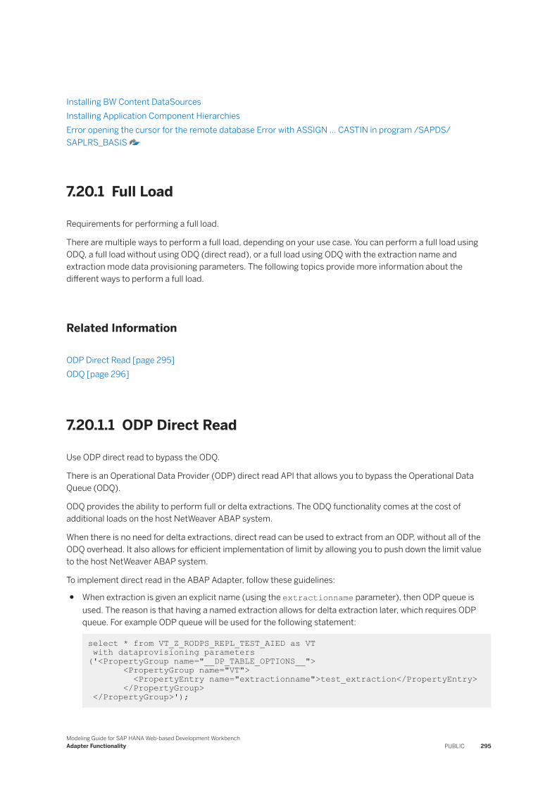
Installing BW Content DataSourcesInstalling Application Component HierarchiesError opening the cursor for the remote database Error with ASSIGN ... CASTIN in program /SAPDS/SAPLRS_BASIS
7.20.1 Full Load
Requirements for performing a full load.
There are multiple ways to perform a full load, depending on your use case. You can perform a full load using ODQ, a full load without using ODQ (direct read), or a full load using ODQ with the extraction name and extraction mode data provisioning parameters. The following topics provide more information about the different ways to perform a full load.
Related Information
ODP Direct Read [page 295]ODQ [page 296]
7.20.1.1 ODP Direct Read
Use ODP direct read to bypass the ODQ.
There is an Operational Data Provider (ODP) direct read API that allows you to bypass the Operational Data Queue (ODQ).
ODQ provides the ability to perform full or delta extractions. The ODQ functionality comes at the cost of additional loads on the host NetWeaver ABAP system.
When there is no need for delta extractions, direct read can be used to extract from an ODP, without all of the ODQ overhead. It also allows for efficient implementation of limit by allowing you to push down the limit value to the host NetWeaver ABAP system.
To implement direct read in the ABAP Adapter, follow these guidelines:
● When extraction is given an explicit name (using the extractionname parameter), then ODP queue is used. The reason is that having a named extraction allows for delta extraction later, which requires ODP queue. For example ODP queue will be used for the following statement:
select * from VT_Z_RODPS_REPL_TEST_AIED as VT with dataprovisioning parameters('<PropertyGroup name="__DP_TABLE_OPTIONS__"> <PropertyGroup name="VT"> <PropertyEntry name="extractionname">test_extraction</PropertyEntry> </PropertyGroup> </PropertyGroup>');
Modeling Guide for SAP HANA Web-based Development WorkbenchAdapter Functionality PUBLIC 295
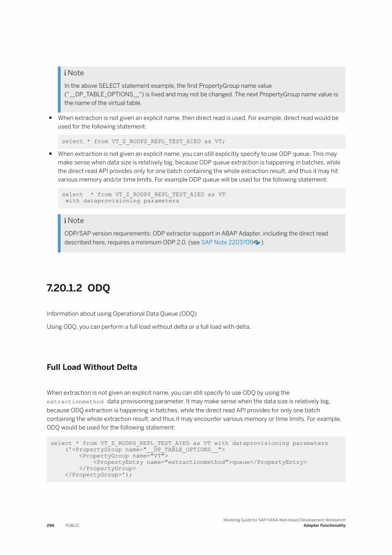
NoteIn the above SELECT statement example, the first PropertyGroup name value ("__DP_TABLE_OPTIONS__") is fixed and may not be changed. The next PropertyGroup name value is the name of the virtual table.
● When extraction is not given an explicit name, then direct read is used. For example, direct read would be used for the following statement:
select * from VT_Z_RODPS_REPL_TEST_AIED as VT;
● When extraction is not given an explicit name, you can still explicitly specify to use ODP queue. This may make sense when data size is relatively big, because ODP queue extraction is happening in batches, while the direct read API provides only for one batch containing the whole extraction result, and thus it may hit various memory and/or time limits. For example ODP queue will be used for the following statement:
select * from VT_Z_RODPS_REPL_TEST_AIED as VT with dataprovisioning parameters
NoteODP/SAP version requirements: ODP extractor support in ABAP Adapter, including the direct read described here, requires a minimum ODP 2.0. (see SAP Note 2203709 )
7.20.1.2 ODQ
Information about using Operational Data Queue (ODQ)
Using ODQ, you can perform a full load without delta or a full load with delta.
Full Load Without Delta
When extraction is not given an explicit name, you can still specify to use ODQ by using the extractionmethod data provisioning parameter. It may make sense when the data size is relatively big, because ODQ extraction is happening in batches, while the direct read API provides for only one batch containing the whole extraction result, and thus it may encounter various memory or time limits. For example, ODQ would be used for the following statement:
select * from VT_Z_RODPS_REPL_TEST_AIED as VT with dataprovisioning parameters ('<PropertyGroup name="__DP_TABLE_OPTIONS__"> <PropertyGroup name="VT"> <PropertyEntry name="extractionmethod">queue</PropertyEntry> </PropertyGroup> </PropertyGroup>');
296 PUBLICModeling Guide for SAP HANA Web-based Development Workbench
Adapter Functionality
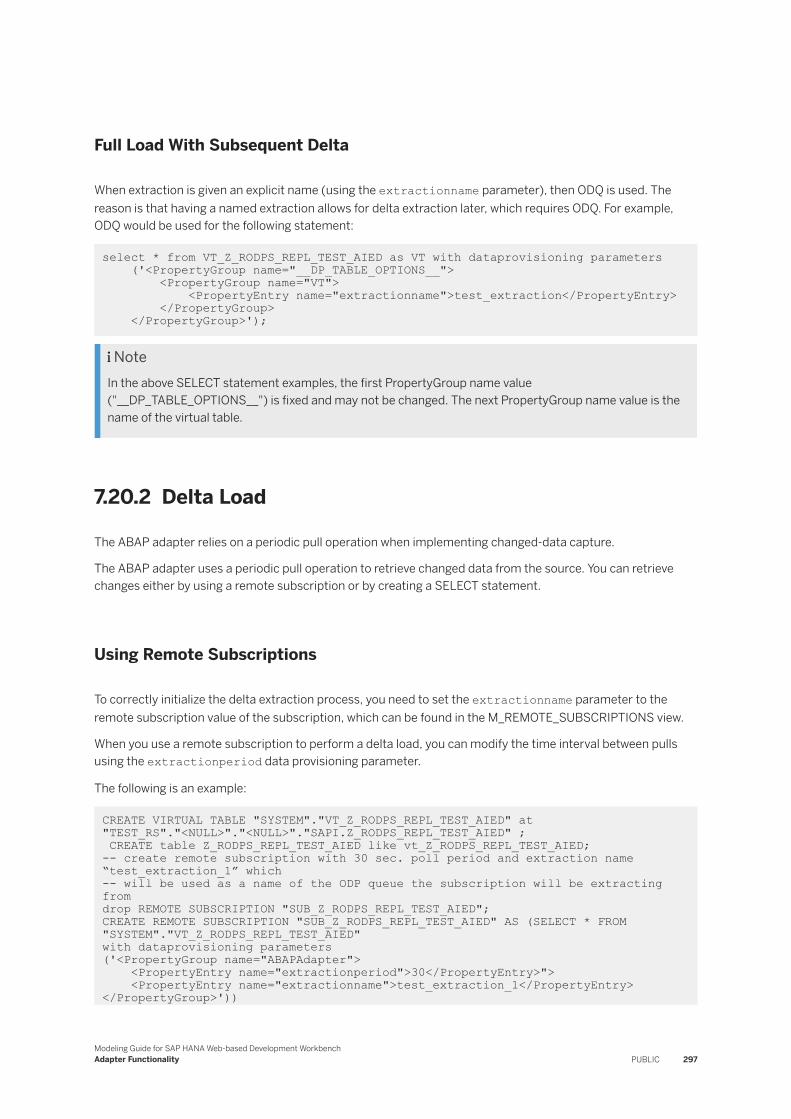
Full Load With Subsequent Delta
When extraction is given an explicit name (using the extractionname parameter), then ODQ is used. The reason is that having a named extraction allows for delta extraction later, which requires ODQ. For example, ODQ would be used for the following statement:
select * from VT_Z_RODPS_REPL_TEST_AIED as VT with dataprovisioning parameters ('<PropertyGroup name="__DP_TABLE_OPTIONS__"> <PropertyGroup name="VT"> <PropertyEntry name="extractionname">test_extraction</PropertyEntry> </PropertyGroup> </PropertyGroup>');
NoteIn the above SELECT statement examples, the first PropertyGroup name value ("__DP_TABLE_OPTIONS__") is fixed and may not be changed. The next PropertyGroup name value is the name of the virtual table.
7.20.2 Delta Load
The ABAP adapter relies on a periodic pull operation when implementing changed-data capture.
The ABAP adapter uses a periodic pull operation to retrieve changed data from the source. You can retrieve changes either by using a remote subscription or by creating a SELECT statement.
Using Remote Subscriptions
To correctly initialize the delta extraction process, you need to set the extractionname parameter to the remote subscription value of the subscription, which can be found in the M_REMOTE_SUBSCRIPTIONS view.
When you use a remote subscription to perform a delta load, you can modify the time interval between pulls using the extractionperiod data provisioning parameter.
The following is an example:
CREATE VIRTUAL TABLE "SYSTEM"."VT_Z_RODPS_REPL_TEST_AIED" at "TEST_RS"."<NULL>"."<NULL>"."SAPI.Z_RODPS_REPL_TEST_AIED" ; CREATE table Z_RODPS_REPL_TEST_AIED like vt_Z_RODPS_REPL_TEST_AIED; -- create remote subscription with 30 sec. poll period and extraction name “test_extraction_1” which-- will be used as a name of the ODP queue the subscription will be extracting fromdrop REMOTE SUBSCRIPTION "SUB_Z_RODPS_REPL_TEST_AIED";CREATE REMOTE SUBSCRIPTION "SUB_Z_RODPS_REPL_TEST_AIED" AS (SELECT * FROM "SYSTEM"."VT_Z_RODPS_REPL_TEST_AIED" with dataprovisioning parameters ('<PropertyGroup name="ABAPAdapter"> <PropertyEntry name="extractionperiod">30</PropertyEntry>"> <PropertyEntry name="extractionname">test_extraction_1</PropertyEntry></PropertyGroup>'))
Modeling Guide for SAP HANA Web-based Development WorkbenchAdapter Functionality PUBLIC 297
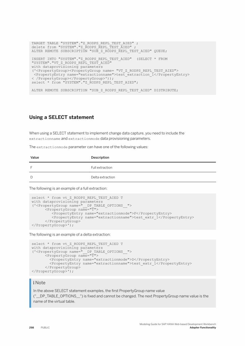
TARGET TABLE "SYSTEM"."Z_RODPS_REPL_TEST_AIED" ;delete from "SYSTEM"."Z_RODPS_REPL_TEST_AIED" ;ALTER REMOTE SUBSCRIPTION "SUB_Z_RODPS_REPL_TEST_AIED" QUEUE; INSERT INTO "SYSTEM"."Z_RODPS_REPL_TEST_AIED" (SELECT * FROM "SYSTEM"."VT_Z_RODPS_REPL_TEST_AIED" with dataprovisioning parameters ('<PropertyGroup><PropertyGroup name= "VT_Z_RODPS_REPL_TEST_AIED"> <PropertyEntry name="extractionname">test_extraction_1</PropertyEntry>< /PropertyGroup></PropertyGroup>'));select * from "SYSTEM"."Z_RODPS_REPL_TEST_AIED"; ALTER REMOTE SUBSCRIPTION "SUB_Z_RODPS_REPL_TEST_AIED" DISTRIBUTE;
Using a SELECT statement
When using a SELECT statement to implement change data capture, you need to include the extractionname and extractionmode data provisioning parameters.
The extractionmode parameter can have one of the following values:
Value Description
F Full extraction
D Delta extraction
The following is an example of a full extraction:
select * from vt_Z_RODPS_REPL_TEST_AIED T with dataprovisioning parameters ('<PropertyGroup name="__DP_TABLE_OPTIONS__"> <PropertyGroup name="T"> <PropertyEntry name="extractionmode">F</PropertyEntry> <PropertyEntry name="extractionname">test_extr_1</PropertyEntry> </PropertyGroup></PropertyGroup>');
The following is an example of a delta extraction:
select * from vt_Z_RODPS_REPL_TEST_AIED T with dataprovisioning parameters ('<PropertyGroup name="__DP_TABLE_OPTIONS__"> <PropertyGroup name="T"> <PropertyEntry name="extractionmode">D</PropertyEntry> <PropertyEntry name="extractionname">test_extr_1</PropertyEntry> </PropertyGroup></PropertyGroup>');
NoteIn the above SELECT statement examples, the first PropertyGroup name value ("__DP_TABLE_OPTIONS__") is fixed and cannot be changed. The next PropertyGroup name value is the name of the virtual table.
298 PUBLICModeling Guide for SAP HANA Web-based Development Workbench
Adapter Functionality
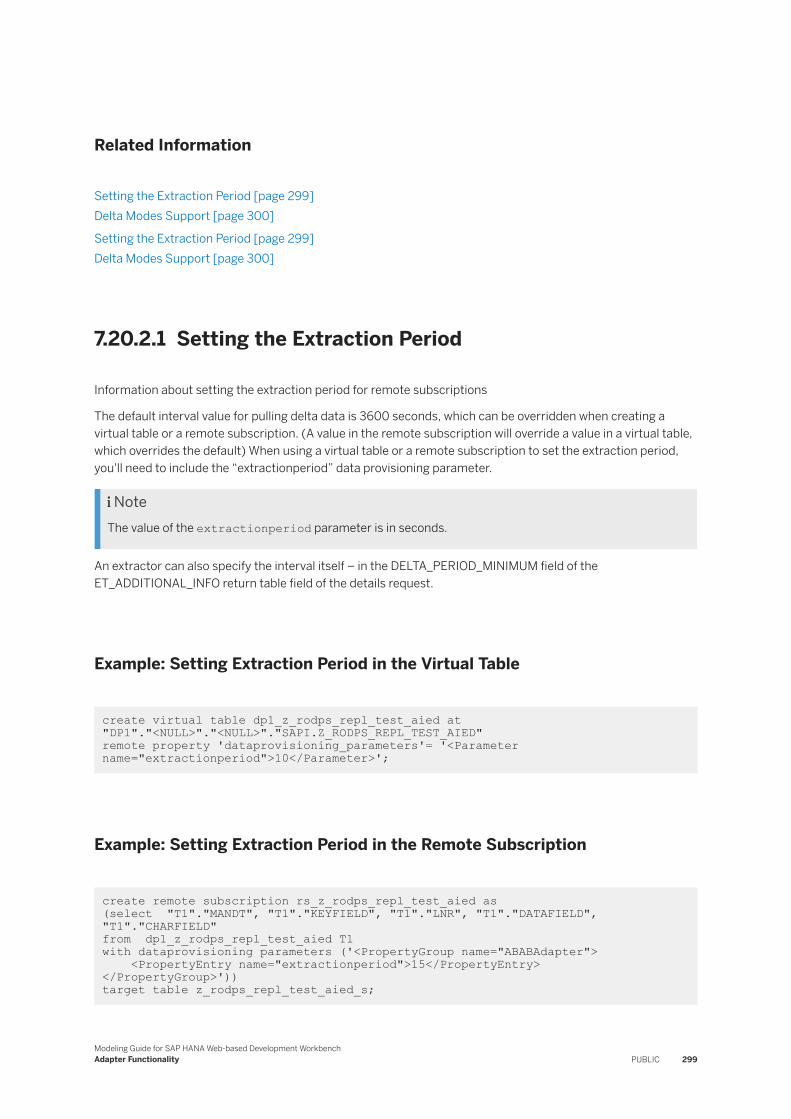
Related Information
Setting the Extraction Period [page 299]Delta Modes Support [page 300]
Setting the Extraction Period [page 299]Delta Modes Support [page 300]
7.20.2.1 Setting the Extraction Period
Information about setting the extraction period for remote subscriptions
The default interval value for pulling delta data is 3600 seconds, which can be overridden when creating a virtual table or a remote subscription. (A value in the remote subscription will override a value in a virtual table, which overrides the default) When using a virtual table or a remote subscription to set the extraction period, you'll need to include the “extractionperiod” data provisioning parameter.
NoteThe value of the extractionperiod parameter is in seconds.
An extractor can also specify the interval itself – in the DELTA_PERIOD_MINIMUM field of the ET_ADDITIONAL_INFO return table field of the details request.
Example: Setting Extraction Period in the Virtual Table
create virtual table dp1_z_rodps_repl_test_aied at "DP1"."<NULL>"."<NULL>"."SAPI.Z_RODPS_REPL_TEST_AIED" remote property 'dataprovisioning_parameters'= '<Parameter name="extractionperiod">10</Parameter>';
Example: Setting Extraction Period in the Remote Subscription
create remote subscription rs_z_rodps_repl_test_aied as (select "T1"."MANDT", "T1"."KEYFIELD", "T1"."LNR", "T1"."DATAFIELD", "T1"."CHARFIELD" from dp1_z_rodps_repl_test_aied T1with dataprovisioning parameters ('<PropertyGroup name="ABABAdapter"> <PropertyEntry name="extractionperiod">15</PropertyEntry></PropertyGroup>')) target table z_rodps_repl_test_aied_s;
Modeling Guide for SAP HANA Web-based Development WorkbenchAdapter Functionality PUBLIC 299
7.20.2.2 Delta Modes Support
The RODPS supports the following delta modes:
● A: ALE Update Pointer (Master Data)● ABR: Complete Delta with Deletion Flag Via Delta Queue (Cube-Compatible)● ABR1: Like Method ABR But Serialization Only by Requests● AIE: After-Images Via Extractor (FI-GL/AP/AR)● AIED: After-Images with Deletion Flag Via Extractor (FI-GL/AP/AR)● AIM: After-Images Via Delta Queue (for example, FI-AP/AR)● AIMD: After-Images with Deletion Flag Via Delta Queue (for example, BtB)● E: Unspecific Delta Via Extractor (Not ODS-Compatible) |● FIL0: Delta Via File Import with After-Images● NEWD: Only New Records (Inserts) Via Delta Queue (Cube-Compatible)● NEWE: Only New Records (Inserts) Via Extractor (Cube-Compatible)● ODS: ODS Extraction
7.20.3 Field Delimited Extraction
Use field delimited extraction for when your tables' fields are of type STRING.
Field delimited extraction will always be used when one or more fields being extracted is a non fixed-length field (that is, defined in the ABAP dictionary as of STRING datatype with 0 length.
Field delimited extraction will not be used, even when the field delimiter is explicitly specified by the user, when all fields are fixed-length fields.
You can explicity specify the delimiter to be used by using the fielddelimiter data provisioning property.
The field delimiter must be exactly one character; the value that you specify will be validated for that, and an error will be thrown upon failure of the validation. If you do not explicitly specify a field delimiter, the default field delimiter (ASCII code 127) will be used when necessary.
The field delimiter can be specified on a virtual table as well as in a select query. The latter takes precedence over the former. Examples:
Virtual table:
create virtual table vt_ODQSSNQUE at "DP8"."<NULL>"."<NULL>"."ABAPTABLES.ODQSSNQUE" remote property 'dataprovisioning_parameters'= '<Parameter name="fielddelimiter">|</Parameter>';
SELECT statement:
select * from vt_ODQSSNQUE T with dataprovisioning parameters ('<PropertyGroup><PropertyGroup name="T"> <PropertyEntry name="fielddelimiter">|</PropertyEntry></PropertyGroup></PropertyGroup>');
300 PUBLICModeling Guide for SAP HANA Web-based Development Workbench
Adapter Functionality
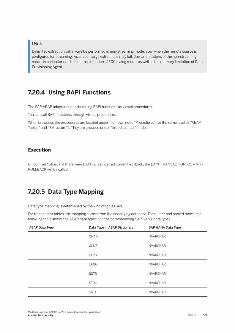
NoteDelimited extraction will always be performed in non-streaming mode, even when the remote source is configured for streaming. As a result large extractions may fail, due to limitations of the non-streaming mode, in particular due to the time limitation of ECC dialog mode, as well as the memory limitation of Data Provisioning Agent.
7.20.4 Using BAPI Functions
The SAP ABAP adapter supports calling BAPI functions as virtual procedures.
You can call BAPI functions through virtual procedures.
When browsing, the procedures are located under their own node "Procedures" (at the same level as “ABAP Tables” and “Extractors”). They are grouped under “first character” nodes.
Execution
On commit/rollback, if there were BAPI calls since last commit/rollback, the BAPI_TRANSACTION_COMMIT/ROLLBACK will be called.
7.20.5 Data Type Mapping
Data type mapping is determined by the kind of table used.
For transparent tables, the mapping comes from the underlying database. For cluster and pooled tables, the following table shows the ABAP data types and the corresponding SAP HANA data types.
ABAP Data Type Data Type in ABAP Dictionary SAP HANA Data Type
CHAR NVARCHAR
CLNT NVARCHAR
CUKY NVARCHAR
LANG NVARCHAR
SSTR NVARCHAR
STRG NVARCHAR
UNIT NVARCHAR
Modeling Guide for SAP HANA Web-based Development WorkbenchAdapter Functionality PUBLIC 301
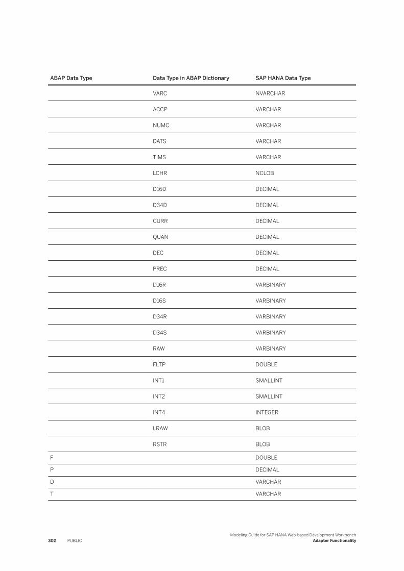
ABAP Data Type Data Type in ABAP Dictionary SAP HANA Data Type
VARC NVARCHAR
ACCP VARCHAR
NUMC VARCHAR
DATS VARCHAR
TIMS VARCHAR
LCHR NCLOB
D16D DECIMAL
D34D DECIMAL
CURR DECIMAL
QUAN DECIMAL
DEC DECIMAL
PREC DECIMAL
D16R VARBINARY
D16S VARBINARY
D34R VARBINARY
D34S VARBINARY
RAW VARBINARY
FLTP DOUBLE
INT1 SMALLINT
INT2 SMALLINT
INT4 INTEGER
LRAW BLOB
RSTR BLOB
F DOUBLE
P DECIMAL
D VARCHAR
T VARCHAR
302 PUBLICModeling Guide for SAP HANA Web-based Development Workbench
Adapter Functionality
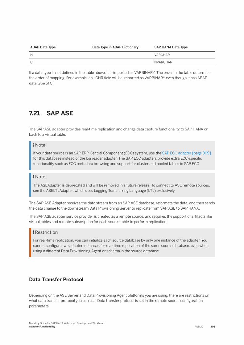
ABAP Data Type Data Type in ABAP Dictionary SAP HANA Data Type
N VARCHAR
C NVARCHAR
If a data type is not defined in the table above, it is imported as VARBINARY. The order in the table determines the order of mapping. For example, an LCHR field will be imported as VARBINARY even though it has ABAP data type of C.
7.21 SAP ASE
The SAP ASE adapter provides real-time replication and change data capture functionality to SAP HANA or back to a virtual table.
NoteIf your data source is an SAP ERP Central Component (ECC) system, use the SAP ECC adapter [page 309] for this database instead of the log reader adapter. The SAP ECC adapters provide extra ECC-specific functionality such as ECC metadata browsing and support for cluster and pooled tables in SAP ECC.
NoteThe ASEAdapter is deprecated and will be removed in a future release. To connect to ASE remote sources, see the ASELTLAdapter, which uses Logging Transferring Language (LTL) exclusively.
The SAP ASE Adapter receives the data stream from an SAP ASE database, reformats the data, and then sends the data change to the downstream Data Provisioning Server to replicate from SAP ASE to SAP HANA.
The SAP ASE adapter service provider is created as a remote source, and requires the support of artifacts like virtual tables and remote subscription for each source table to perform replication.
RestrictionFor real-time replication, you can initialize each source database by only one instance of the adapter. You cannot configure two adapter instances for real-time replication of the same source database, even when using a different Data Provisioning Agent or schema in the source database.
Data Transfer Protocol
Depending on the ASE Server and Data Provisioning Agent platforms you are using, there are restrictions on what data transfer protocol you can use. Data transfer protocol is set in the remote source configuration parameters.
Modeling Guide for SAP HANA Web-based Development WorkbenchAdapter Functionality PUBLIC 303

ASE Server Platform DP Agent Platform Allowed Data Transfer Protocol
Linux Linux CI and LTL
Linux Linux PPCLE CI and LTL
Linux Windows LTL
Adapter Functionality
The SAP ASE adapter supports the following functionality:
● Virtual table as a source● Real-time change data capture● Virtual table as a target using a Data Sink node in a flowgraph● Loading options for target tables● Search for a table● Replication monitoring and statistics
Real-time Replication Limitations
The following limitations exist when performing real-time replication:
● Unsupported table types:○ Table with all LOB columns○ Table with LOB column and no primary key or unique index○ Table with duplicated rows and no primary key○ Table with minimal logging option
Related Information
SAP ASE to SAP HANA Data Type Mapping [page 304]
Load Behavior Options for Targets in Replication Tasks [page 26]
7.21.1 SAP ASE to SAP HANA Data Type Mapping
The following table shows data type mappings from SAP ASE to SAP HANA.
The SAP ASE adapter supports compressed LOB.
304 PUBLICModeling Guide for SAP HANA Web-based Development Workbench
Adapter Functionality

SAP ASE Data Type SAP HANA Data Type
BIGDATETIME TIMESTAMP
BIGINT BIGINT
BIGTIME TIMESTAMP
BINARY VARBINARY
BIT TINYINT
CHAR VARCHAR
DATE DATE
DATETIME TIMESTAMP
DECIMAL DECIMAL
DOUBLE PRECISION DOUBLE
FLOAT DOUBLE
IDENTITY DOUBLE
INT INTEGER
IMAGE BLOB
LONGSYSNAME VARCHAR (255)
MONEY DECIMAL (19,4)
NCHAR NVARCHAR
NUMERIC DECIMAL
NVARCHAR NVARCHAR
REAL REAL
SMALLDATETIME TIMESTAMP
SMALLINT SMALLINT
SMALLMONEY DECIMAL (10,4)
SYSNAME VARCHAR (3)
TEXT CLOB
TIMESTAMP VARBINARY (8)
Modeling Guide for SAP HANA Web-based Development WorkbenchAdapter Functionality PUBLIC 305
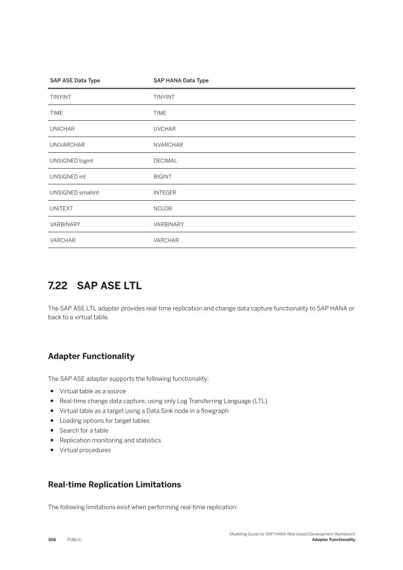
SAP ASE Data Type SAP HANA Data Type
TINYINT TINYINT
TIME TIME
UNICHAR UVCHAR
UNIVARCHAR NVARCHAR
UNSIGNED bigint DECIMAL
UNSIGNED int BIGINT
UNSIGNED smallint INTEGER
UNITEXT NCLOB
VARBINARY VARBINARY
VARCHAR VARCHAR
7.22 SAP ASE LTL
The SAP ASE LTL adapter provides real-time replication and change data capture functionality to SAP HANA or back to a virtual table.
Adapter Functionality
The SAP ASE adapter supports the following functionality:
● Virtual table as a source● Real-time change data capture, using only Log Transferring Language (LTL)● Virtual table as a target using a Data Sink node in a flowgraph● Loading options for target tables● Search for a table● Replication monitoring and statistics● Virtual procedures
Real-time Replication Limitations
The following limitations exist when performing real-time replication:
306 PUBLICModeling Guide for SAP HANA Web-based Development Workbench
Adapter Functionality
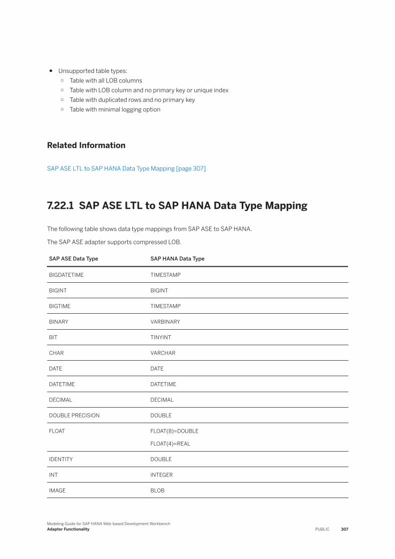
● Unsupported table types:○ Table with all LOB columns○ Table with LOB column and no primary key or unique index○ Table with duplicated rows and no primary key○ Table with minimal logging option
Related Information
SAP ASE LTL to SAP HANA Data Type Mapping [page 307]
7.22.1 SAP ASE LTL to SAP HANA Data Type Mapping
The following table shows data type mappings from SAP ASE to SAP HANA.
The SAP ASE adapter supports compressed LOB.
SAP ASE Data Type SAP HANA Data Type
BIGDATETIME TIMESTAMP
BIGINT BIGINT
BIGTIME TIMESTAMP
BINARY VARBINARY
BIT TINYINT
CHAR VARCHAR
DATE DATE
DATETIME DATETIME
DECIMAL DECIMAL
DOUBLE PRECISION DOUBLE
FLOAT FLOAT(8)=DOUBLE
FLOAT(4)=REAL
IDENTITY DOUBLE
INT INTEGER
IMAGE BLOB
Modeling Guide for SAP HANA Web-based Development WorkbenchAdapter Functionality PUBLIC 307

SAP ASE Data Type SAP HANA Data Type
LONGSYSNAME VARCHAR (255)
MONEY DECIMAL
NCHAR NVARCHAR
NUMERIC NUMERIC
NVARCHAR NVARCHAR
REAL REAL
SMALLDATETIME SECONDDATE
SMALLINT SMALLINT
SMALLMONEY REAL
SYSNAME VARCHAR (3)
TEXT CLOB
TIMESTAMP VARBINARY (8)
TINYINT TINYINT
TIME TIME
UNICHAR NVARCHAR
UNIVARCHAR NVARCHAR
UNSIGNED bigint DECIMAL
UNSIGNED int BIGINT
UNSIGNED smallint INTEGER
UNITEXT NCLOB
VARBINARY VARBINARY
VARCHAR VARCHAR
308 PUBLICModeling Guide for SAP HANA Web-based Development Workbench
Adapter Functionality
7.23 SAP ECC
SAP ERP Central Component (ECC) adapters are a set of data provisioning adapters to provide access to and interaction with SAP ECC data and metadata.
All adapters designed to work with SAP ECC are built on top of Data Provisioning log reader adapters for the same database. Currently supported are the following:
● IBM DB2● Oracle
NoteThe Oracle Log Miner maximum throughput is approximately 1 TB per day; therefore, for replication volumes greater than 1 TB per day, expect delays in replication.
● Microsoft SQL Server● SAP ASE● SAP ASE LTL
These adapters provide extra ECC-specific functionality: ECC metadata browsing and support for cluster tables and pooled tables in SAP ECC. Please see the description of Log Reader adapters for the common functionality.
NoteFor IBM DB2, Oracle, and Microsoft SQL Server (does not apply to SAP ASE), before registering the adapter with the SAP HANA system, download and install the correct JDBC libraries. See the SAP HANA smart data integration Product Availability Matrix (PAM). In the <DPAgent_root> folder, create a /lib
Adapter Functionality
The ECC adapters support the following functionality:
● Real-time change-data capture
RestrictionFor real-time replication, you can initialize each source database by only one remote source. You cannot configure two remote sources for real-time replication of the same source database, even when using a different Data Provisioning Agent or schema in the source database.
● DDL propagation (transparent tables only, not supported for SAP ASE ECC)● Search for tables● Agent-stored credentials (not supported for SAP ASE ECC)● SELECT, WHERE, JOIN, GROUP BY, DISTINCT, TOP, LIMIT
Modeling Guide for SAP HANA Web-based Development WorkbenchAdapter Functionality PUBLIC 309
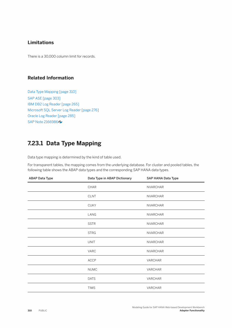
Limitations
There is a 30,000 column limit for records.
Related Information
Data Type Mapping [page 310]
SAP ASE [page 303]IBM DB2 Log Reader [page 265]Microsoft SQL Server Log Reader [page 276]Oracle Log Reader [page 285]SAP Note 2166986
7.23.1 Data Type Mapping
Data type mapping is determined by the kind of table used.
For transparent tables, the mapping comes from the underlying database. For cluster and pooled tables, the following table shows the ABAP data types and the corresponding SAP HANA data types.
ABAP Data Type Data Type in ABAP Dictionary SAP HANA Data Type
CHAR NVARCHAR
CLNT NVARCHAR
CUKY NVARCHAR
LANG NVARCHAR
SSTR NVARCHAR
STRG NVARCHAR
UNIT NVARCHAR
VARC NVARCHAR
ACCP VARCHAR
NUMC VARCHAR
DATS VARCHAR
TIMS VARCHAR
310 PUBLICModeling Guide for SAP HANA Web-based Development Workbench
Adapter Functionality
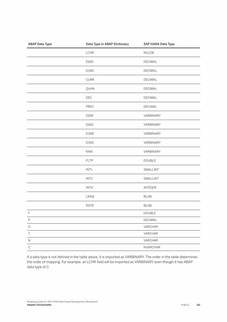
ABAP Data Type Data Type in ABAP Dictionary SAP HANA Data Type
LCHR NCLOB
D16D DECIMAL
D34D DECIMAL
CURR DECIMAL
QUAN DECIMAL
DEC DECIMAL
PREC DECIMAL
D16R VARBINARY
D16S VARBINARY
D34R VARBINARY
D34S VARBINARY
RAW VARBINARY
FLTP DOUBLE
INT1 SMALLINT
INT2 SMALLINT
INT4 INTEGER
LRAW BLOB
RSTR BLOB
F DOUBLE
P DECIMAL
D VARCHAR
T VARCHAR
N VARCHAR
C NVARCHAR
If a data type is not defined in the table above, it is imported as VARBINARY. The order in the table determines the order of mapping. For example, an LCHR field will be imported as VARBINARY even though it has ABAP data type of C.
Modeling Guide for SAP HANA Web-based Development WorkbenchAdapter Functionality PUBLIC 311
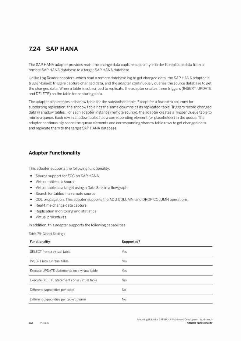
7.24 SAP HANA
The SAP HANA adapter provides real-time change data capture capability in order to replicate data from a remote SAP HANA database to a target SAP HANA database.
Unlike Log Reader adapters, which read a remote database log to get changed data, the SAP HANA adapter is trigger-based: triggers capture changed data, and the adapter continuously queries the source database to get the changed data. When a table is subscribed to replicate, the adapter creates three triggers (INSERT, UPDATE, and DELETE) on the table for capturing data.
The adapter also creates a shadow table for the subscribed table. Except for a few extra columns for supporting replication, the shadow table has the same columns as its replicated table. Triggers record changed data in shadow tables. For each adapter instance (remote source), the adapter creates a Trigger Queue table to mimic a queue. Each row in shadow tables has a corresponding element (or placeholder) in the queue. The adapter continuously scans the queue elements and corresponding shadow table rows to get changed data and replicate them to the target SAP HANA database.
Adapter Functionality
This adapter supports the following functionality:
● Source support for ECC on SAP HANA● Virtual table as a source● Virtual table as a target using a Data Sink in a flowgraph● Search for tables in a remote source● DDL propagation. This adapter supports the ADD COLUMN, and DROP COLUMN operations.● Real-time change data capture● Replication monitoring and statistics● Virtual procedures
In addition, this adapter supports the following capabilities:
Table 79: Global Settings
Functionality Supported?
SELECT from a virtual table Yes
INSERT into a virtual table Yes
Execute UPDATE statements on a virtual table Yes
Execute DELETE statements on a virtual table Yes
Different capabilities per table No
Different capabilities per table column No
312 PUBLICModeling Guide for SAP HANA Web-based Development Workbench
Adapter Functionality
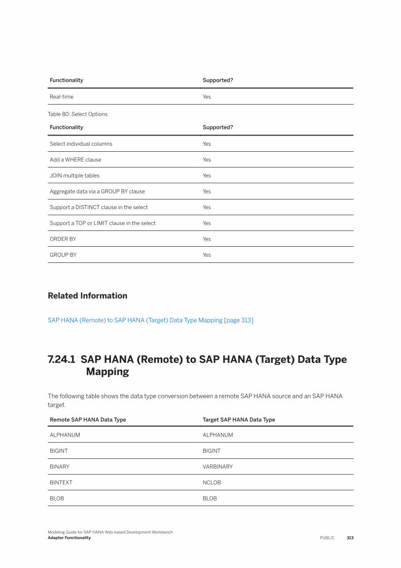
Functionality Supported?
Real-time Yes
Table 80: Select Options
Functionality Supported?
Select individual columns Yes
Add a WHERE clause Yes
JOIN multiple tables Yes
Aggregate data via a GROUP BY clause Yes
Support a DISTINCT clause in the select Yes
Support a TOP or LIMIT clause in the select Yes
ORDER BY Yes
GROUP BY Yes
Related Information
SAP HANA (Remote) to SAP HANA (Target) Data Type Mapping [page 313]
7.24.1 SAP HANA (Remote) to SAP HANA (Target) Data Type Mapping
The following table shows the data type conversion between a remote SAP HANA source and an SAP HANA target.
Remote SAP HANA Data Type Target SAP HANA Data Type
ALPHANUM ALPHANUM
BIGINT BIGINT
BINARY VARBINARY
BINTEXT NCLOB
BLOB BLOB
Modeling Guide for SAP HANA Web-based Development WorkbenchAdapter Functionality PUBLIC 313
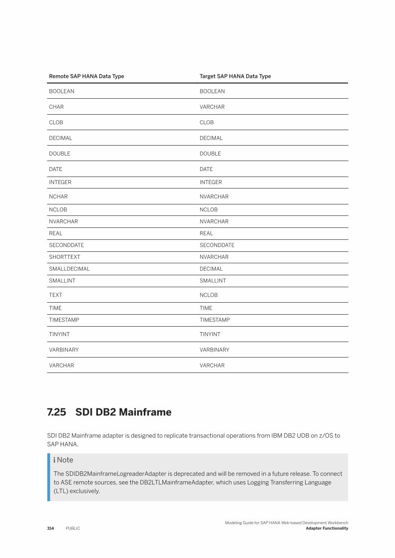
Remote SAP HANA Data Type Target SAP HANA Data Type
BOOLEAN BOOLEAN
CHAR VARCHAR
CLOB CLOB
DECIMAL DECIMAL
DOUBLE DOUBLE
DATE DATE
INTEGER INTEGER
NCHAR NVARCHAR
NCLOB NCLOB
NVARCHAR NVARCHAR
REAL REAL
SECONDDATE SECONDDATE
SHORTTEXT NVARCHAR
SMALLDECIMAL DECIMAL
SMALLINT SMALLINT
TEXT NCLOB
TIME TIME
TIMESTAMP TIMESTAMP
TINYINT TINYINT
VARBINARY VARBINARY
VARCHAR VARCHAR
7.25 SDI DB2 Mainframe
SDI DB2 Mainframe adapter is designed to replicate transactional operations from IBM DB2 UDB on z/OS to SAP HANA.
NoteThe SDIDB2MainframeLogreaderAdapter is deprecated and will be removed in a future release. To connect to ASE remote sources, see the DB2LTLMainframeAdapter, which uses Logging Transferring Language (LTL) exclusively.
314 PUBLICModeling Guide for SAP HANA Web-based Development Workbench
Adapter Functionality
The adapter extracts data from IBM DB2 UDB on z/OS databases as initial load and real-time change data capture.
NoteThe SDI DB2 Mainframe adapter does not come pre-installed with the Data Provisioning Agent; you must install it separately. Before installing the SDI DB2 Mainframe adapter, you must install the Data Provisioning Agent.
This adapter is supported on Linux only.
Adapter Functionality
This adapter supports the following functionality:
● Virtual table as a source
NoteINSERT, UPDATE, and DELETE on a virtual table are not supported.
● Initial load● Real-time change data capture
NoteDDLs are not supported. Also, transactional operations include only INSERT, UPDATE, and DELETE
Encoding schemes supported on the source system: ASCII, EBCDIC, and Unicode
● Replication Monitoring and Statistics● Search for Tables
In addition, this adapter supports the following capabilities:
● SELECT (WHERE, JOIN, GROUP BY, DISTINCT, TOP or LIMIT, ORDER BY)
Related Information
IBM DB2 Mainframe to SAP HANA Data Type Mapping [page 316]
SAP HANA Smart Data Integration and Smart Data Quality Product Availability MatrixReplication Agent OverviewSDI DB2 LTL Mainframe
Modeling Guide for SAP HANA Web-based Development WorkbenchAdapter Functionality PUBLIC 315

7.25.1 IBM DB2 Mainframe to SAP HANA Data Type Mapping
The following table shows the conversion between DB2 Mainframe data types and SAP HANA data types.
DB2 z/OS Data Type SAP HANA Data Type
BIGINT BIGINT
BINARY VARBINARY
BLOB
NoteNot supported for CDC
BLOB
CHAR VARCHAR
CLOB
NoteNot supported for CDC
CLOB
DATE DATE
DBCLOB
NoteNot supported for CDC
CLOB
DECIMAL DECIMAL
DECFLOAT DOUBLE
DOUBLE DOUBLE
GRAPHIC NVARCHAR
INTEGER INTEGER
LONGVARBINARY
NoteNot supported for CDC
BLOB
316 PUBLICModeling Guide for SAP HANA Web-based Development Workbench
Adapter Functionality
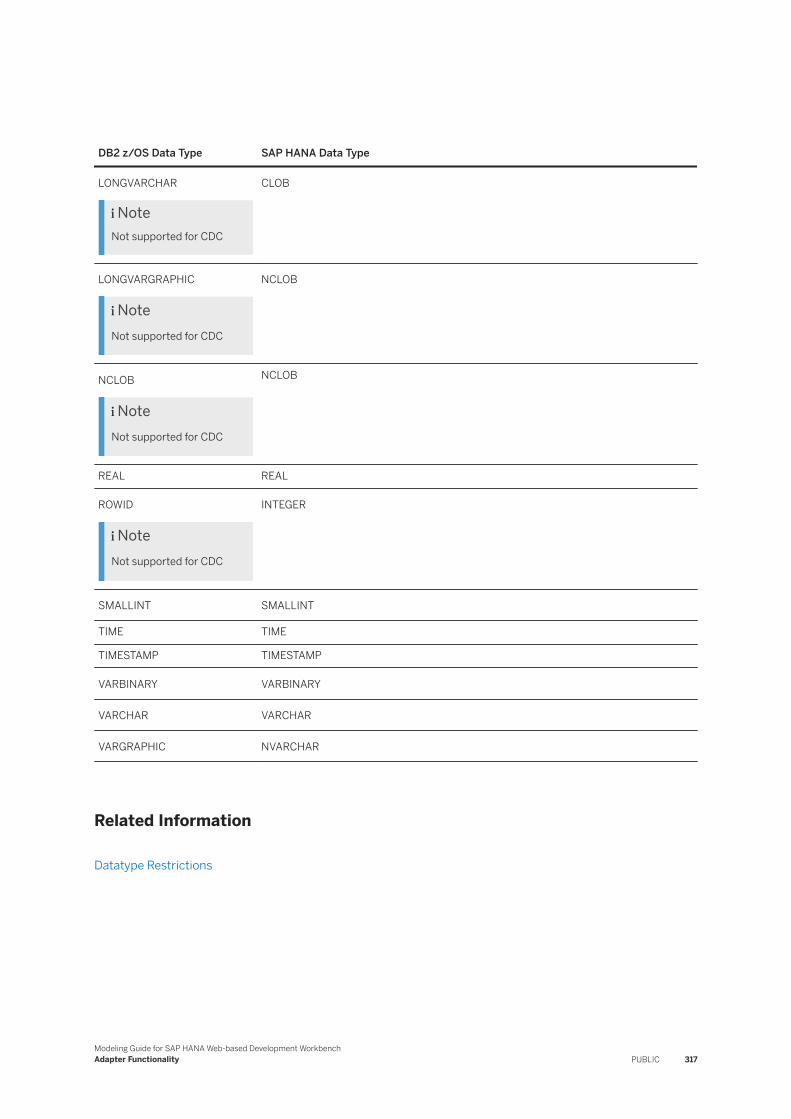
DB2 z/OS Data Type SAP HANA Data Type
LONGVARCHAR
NoteNot supported for CDC
CLOB
LONGVARGRAPHIC
NoteNot supported for CDC
NCLOB
NCLOB
NoteNot supported for CDC
NCLOB
REAL REAL
ROWID
NoteNot supported for CDC
INTEGER
SMALLINT SMALLINT
TIME TIME
TIMESTAMP TIMESTAMP
VARBINARY VARBINARY
VARCHAR VARCHAR
VARGRAPHIC NVARCHAR
Related Information
Datatype Restrictions
Modeling Guide for SAP HANA Web-based Development WorkbenchAdapter Functionality PUBLIC 317
7.26 SOAP
The SOAP adapter provides access to SOAP Web Services via HANA SQL.
The SOAP adapter is a SOAP web services client that can talk to a web service using the HTTP protocol to download the data. The SOAP adapter uses virtual functions instead of virtual tables to expose server-side operations.
The SOAP adapter supports the following functionality:
● Virtual function as a source
Related Information
SOAP Operations as Virtual Function [page 318]Process the Response [page 319]
CREATE VIRTUAL FUNCTION
7.26.1 SOAP Operations as Virtual Function
Create a virtual function to retrieve data.
SOAP web service browsing will display all of the operations as a leaf node. Because SOAP requests and responses are both XML messages, you will use the Hierarchical node in a flowgraph, with the virtual function as your source. You will use Virtual Function Configuration to keep the root schemas and referenced schemas from the WSDL file. Use the GET_REMOTE_SOURCE_FUNCTION_DEFINITION procedure, and as part of this call, the SOAP adapter will provide the following information to SAP HANA.
NoteYou can only create virtual function using SQL or the Web-based Development Workbench. We provide sample SQL code here. For more information about creating a virtual function using the Web-based Development Workbench, see the Modeling Guide for SAP HANA Smart Data Integration and SAP HANA Smart Data Quality.
318 PUBLICModeling Guide for SAP HANA Web-based Development Workbench
Adapter Functionality
7.26.2 Process the Response
Process the SOAP response using the Hierarchical node.
Context
You have created a virtual function, and now you can process the response using the Hierarchical node in the Web-based Development Workbench.
Procedure
1. Open the Catalog editor and import the virtual function you want to execute.2. Configure the remote source to use the imported virtual function.3. Add a Hierarchical node to the flowgraph, connect it to the data source, and configure the node.4. Add a target table to the flowgraph, connect it upstream, and name it.5. Save the flowgraph, and execute it.6. Click the Data Preview button on the target table to confirm that the data is saved correctly.
Related Information
Hierarchical [page 179]
7.27 Teradata
The Teradata adapter can be used to connect to a Teradata remote source and create a virtual table to read from and write to.
Adapter Functionality
This adapter supports the following functionality:
● Virtual table as a source● Real-time change data capture● Search for tables
Modeling Guide for SAP HANA Web-based Development WorkbenchAdapter Functionality PUBLIC 319
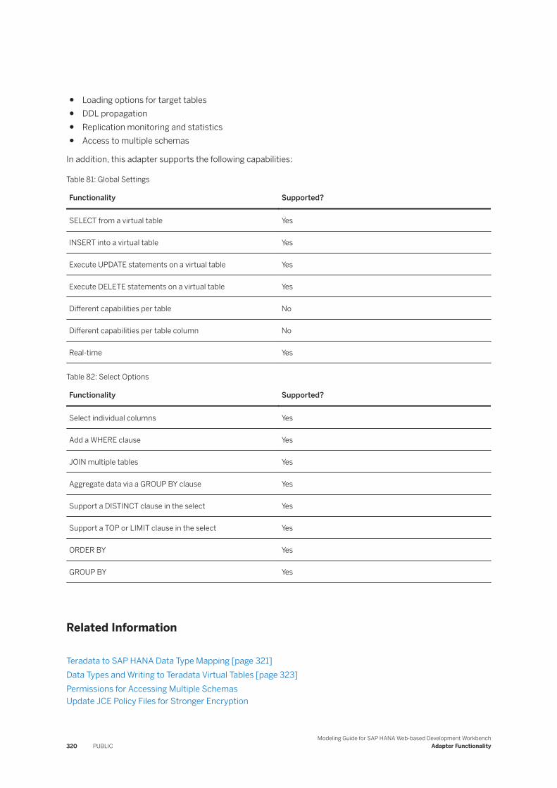
● Loading options for target tables● DDL propagation● Replication monitoring and statistics● Access to multiple schemas
In addition, this adapter supports the following capabilities:
Table 81: Global Settings
Functionality Supported?
SELECT from a virtual table Yes
INSERT into a virtual table Yes
Execute UPDATE statements on a virtual table Yes
Execute DELETE statements on a virtual table Yes
Different capabilities per table No
Different capabilities per table column No
Real-time Yes
Table 82: Select Options
Functionality Supported?
Select individual columns Yes
Add a WHERE clause Yes
JOIN multiple tables Yes
Aggregate data via a GROUP BY clause Yes
Support a DISTINCT clause in the select Yes
Support a TOP or LIMIT clause in the select Yes
ORDER BY Yes
GROUP BY Yes
Related Information
Teradata to SAP HANA Data Type Mapping [page 321]Data Types and Writing to Teradata Virtual Tables [page 323]Permissions for Accessing Multiple SchemasUpdate JCE Policy Files for Stronger Encryption
320 PUBLICModeling Guide for SAP HANA Web-based Development Workbench
Adapter Functionality
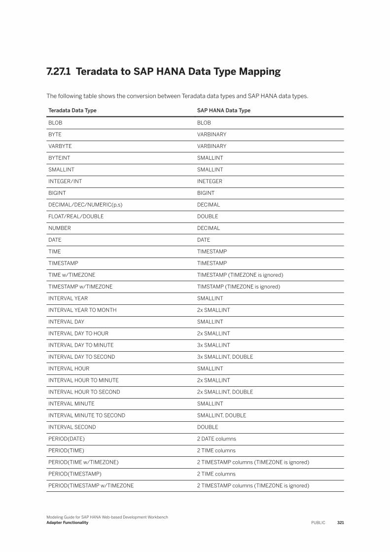
7.27.1 Teradata to SAP HANA Data Type Mapping
The following table shows the conversion between Teradata data types and SAP HANA data types.
Teradata Data Type SAP HANA Data Type
BLOB BLOB
BYTE VARBINARY
VARBYTE VARBINARY
BYTEINT SMALLINT
SMALLINT SMALLINT
INTEGER/INT INETEGER
BIGINT BIGINT
DECIMAL/DEC/NUMERIC(p,s) DECIMAL
FLOAT/REAL/DOUBLE DOUBLE
NUMBER DECIMAL
DATE DATE
TIME TIMESTAMP
TIMESTAMP TIMESTAMP
TIME w/TIMEZONE TIMESTAMP (TIMEZONE is ignored)
TIMESTAMP w/TIMEZONE TIMSTAMP (TIMEZONE is ignored)
INTERVAL YEAR SMALLINT
INTERVAL YEAR TO MONTH 2x SMALLINT
INTERVAL DAY SMALLINT
INTERVAL DAY TO HOUR 2x SMALLINT
INTERVAL DAY TO MINUTE 3x SMALLINT
INTERVAL DAY TO SECOND 3x SMALLINT, DOUBLE
INTERVAL HOUR SMALLINT
INTERVAL HOUR TO MINUTE 2x SMALLINT
INTERVAL HOUR TO SECOND 2x SMALLINT, DOUBLE
INTERVAL MINUTE SMALLINT
INTERVAL MINUTE TO SECOND SMALLINT, DOUBLE
INTERVAL SECOND DOUBLE
PERIOD(DATE) 2 DATE columns
PERIOD(TIME) 2 TIME columns
PERIOD(TIME w/TIMEZONE) 2 TIMESTAMP columns (TIMEZONE is ignored)
PERIOD(TIMESTAMP) 2 TIME columns
PERIOD(TIMESTAMP w/TIMEZONE 2 TIMESTAMP columns (TIMEZONE is ignored)
Modeling Guide for SAP HANA Web-based Development WorkbenchAdapter Functionality PUBLIC 321
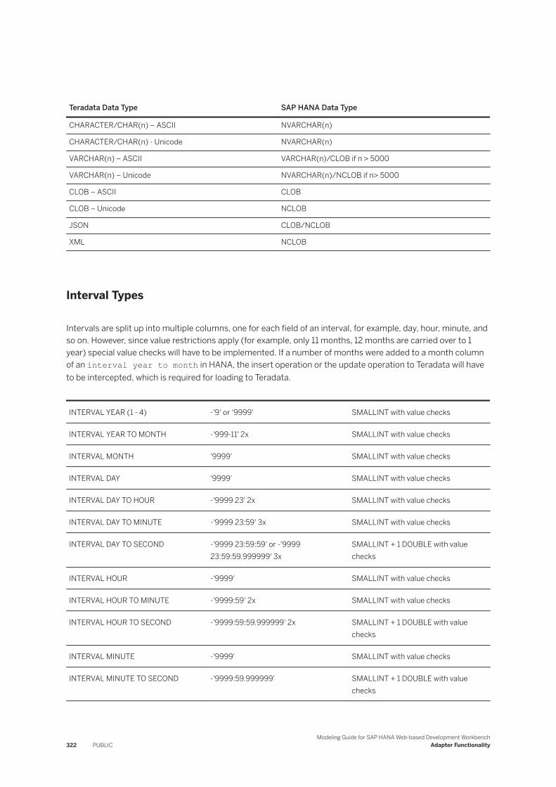
Teradata Data Type SAP HANA Data Type
CHARACTER/CHAR(n) – ASCII NVARCHAR(n)
CHARACTER/CHAR(n) - Unicode NVARCHAR(n)
VARCHAR(n) – ASCII VARCHAR(n)/CLOB if n > 5000
VARCHAR(n) – Unicode NVARCHAR(n)/NCLOB if n> 5000
CLOB – ASCII CLOB
CLOB – Unicode NCLOB
JSON CLOB/NCLOB
XML NCLOB
Interval Types
Intervals are split up into multiple columns, one for each field of an interval, for example, day, hour, minute, and so on. However, since value restrictions apply (for example, only 11 months, 12 months are carried over to 1 year) special value checks will have to be implemented. If a number of months were added to a month column of an interval year to month in HANA, the insert operation or the update operation to Teradata will have to be intercepted, which is required for loading to Teradata.
INTERVAL YEAR (1 - 4) -'9' or '9999' SMALLINT with value checks
INTERVAL YEAR TO MONTH -'999-11' 2x SMALLINT with value checks
INTERVAL MONTH '9999' SMALLINT with value checks
INTERVAL DAY '9999' SMALLINT with value checks
INTERVAL DAY TO HOUR -'9999 23' 2x SMALLINT with value checks
INTERVAL DAY TO MINUTE -'9999 23:59' 3x SMALLINT with value checks
INTERVAL DAY TO SECOND -'9999 23:59:59' or -'9999 23:59:59.999999' 3x
SMALLINT + 1 DOUBLE with value checks
INTERVAL HOUR -'9999' SMALLINT with value checks
INTERVAL HOUR TO MINUTE -'9999:59' 2x SMALLINT with value checks
INTERVAL HOUR TO SECOND -'9999:59:59.999999' 2x SMALLINT + 1 DOUBLE with value checks
INTERVAL MINUTE -'9999' SMALLINT with value checks
INTERVAL MINUTE TO SECOND -'9999:59.999999' SMALLINT + 1 DOUBLE with value checks
322 PUBLICModeling Guide for SAP HANA Web-based Development Workbench
Adapter Functionality

INTERVAL SECOND -'9999.999999' DOUBLE with value checks
Related Information
Data Types and Writing to Teradata Virtual Tables [page 323]
7.27.2 Data Types and Writing to Teradata Virtual Tables
When writing to a virtual table, keep in mind that there are special considerations related to data types, depending on the operation you use.
INSERT
Inserting values into a Teradata backed virtual table comes with some restrictions:
Column data type Notes
Period Period columns are split into two columns in SAP HANA (begin and ending bound of the time period). Because the adapter will reconstruct a Teradata period under the hood from these values, Teradata restrictions on periods apply for these columns in SAP HANA, as well. Otherwise, the insert will fail. For example:
● The ending bound value has to be greater than the beginning value.● Null values in the ending bound are not allowed for time periods.
Interval ● All columns have to be included in the insert statement and assigned values.● If the resulting interval should be negative, all values of the interval have to be nega
tive; no mixing of signs is allowed. This mirrors the behavior of selecting values from negative periods; think additive behavior of the values.
● If the resulting interval should be null, all values have to be null.● Some values have restricted ranges. For example, the minute column (in SAPA HANA)
of a minute to second interval (in Teradata) can only have values in the range of -59 <= x <= 59, even though the minute part may be represented by a smallint column in SAP HANA. See the Teradata documentations for allowed values.
Modeling Guide for SAP HANA Web-based Development WorkbenchAdapter Functionality PUBLIC 323
UPDATE
When updating interval columns, all columns and values have to be specified (see below), because Teradata does not allow partial updates of intervals.
Sample Code
update "SYSTEM"."local_a_target_interval" set "i_day_minute_DAY"=5, "i_day_minute_HOUR"=6, "i_day_minute_MINUTE"=8;
The same value restrictions as for insert apply:
● To make the overall interval null, all interval values have to be set to null● To make the interval negative, all values have to be negative
Related Information
Teradata to SAP HANA Data Type Mapping [page 321]
7.28 Twitter
The Twitter adapter provides access to Twitter data via the Data Provisioning Agent.
Twitter is a social media Web site that hosts millions of tweets every day. The Twitter platform provides access to this corpus of data. Twitter has exposed all its data via RESTful API so that it can be consumed with any HTTP client. Twitter APIs allow you to consume tweets in different ways, from getting tweets from a specific user, to performing a public search, or subscribing to real-time feeds for specific users or the entire Twitter community.
Adapter Functionality
The Twitter adapter supports the following functionality:
● Virtual table or function as a source● Real-time change data capture (flowgraph and replication task)
In addition, this adapter supports the following capabilities:
● SELECT, WHERE
324 PUBLICModeling Guide for SAP HANA Web-based Development Workbench
Adapter Functionality
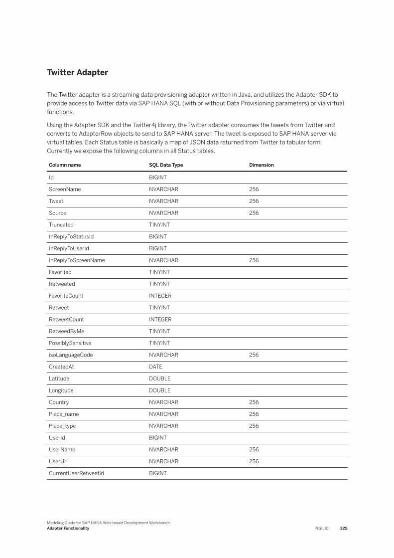
Twitter Adapter
The Twitter adapter is a streaming data provisioning adapter written in Java, and utilizes the Adapter SDK to provide access to Twitter data via SAP HANA SQL (with or without Data Provisioning parameters) or via virtual functions.
Using the Adapter SDK and the Twitter4j library, the Twitter adapter consumes the tweets from Twitter and converts to AdapterRow objects to send to SAP HANA server. The tweet is exposed to SAP HANA server via virtual tables. Each Status table is basically a map of JSON data returned from Twitter to tabular form. Currently we expose the following columns in all Status tables.
Column name SQL Data Type Dimension
Id BIGINT
ScreenName NVARCHAR 256
Tweet NVARCHAR 256
Source NVARCHAR 256
Truncated TINYINT
InReplyToStatusId BIGINT
InReplyToUserId BIGINT
InReplyToScreenName NVARCHAR 256
Favorited TINYINT
Retweeted TINYINT
FavoriteCount INTEGER
Retweet TINYINT
RetweetCount INTEGER
RetweedByMe TINYINT
PossiblySensitive TINYINT
isoLanguageCode NVARCHAR 256
CreatedAt DATE
Latitude DOUBLE
Longitude DOUBLE
Country NVARCHAR 256
Place_name NVARCHAR 256
Place_type NVARCHAR 256
UserId BIGINT
UserName NVARCHAR 256
UserUrl NVARCHAR 256
CurrentUserRetweetId BIGINT
Modeling Guide for SAP HANA Web-based Development WorkbenchAdapter Functionality PUBLIC 325

Related Information
Twitter Terminology [page 326]Creating Twitter Virtual Tables and Functions [page 327]Restrictions and Limitations [page 336]
7.28.1 Twitter Terminology
Understanding Twitter terminology helps you get the most out of Twitter data.
The following is a brief list of relevant Twitter terms:
Term Definition
Home timeline The home timeline is the tweets that appear in your home page when you log in. It returns a collection of the most recent tweets and retweets posted by the authenticating user and the users they follow. It will contain tweets that you follow, or those that you have tweeted, retweeted, replied to, favorited, mentioned, and so on.
User timeline User timeline returns a collection of the most recent tweets posted by the user indicated by the screen name. The timeline returned is the equivalent of the one seen when you view a user’s profile on twitter.com.
When you specify a different user (other than authenticating user), the user timeline returns the tweets that are posted by that user. This is similar to that user’s profile on Twitter.com. Each user has a user name or in Twitter it is known as screen name. This is the same name that appears after @, used to refer/mention a user.
Search tweets Searching tweets (formerly known as Public Timeline) allows you to query for all tweets posted by all the users of Twitter. It returns a collection of relevant tweets matching a specified query.
User stream User streams provide a way for a single user to be streamed the equivalent of their home timeline (the tweets authored by the users they follow) and mentions timeline (the tweets authored by users @mentioning that user).
Public stream This stream returns public statuses (public data flowing through Twitter) that match one or more filter predicates.
For more information, see the Twitter documentation.
326 PUBLICModeling Guide for SAP HANA Web-based Development Workbench
Adapter Functionality

Related Information
https://developer.twitter.com/en
7.28.2 Creating Twitter Virtual Tables and Functions
Depending on your needs, you need to create either a virtual table or virtual function to access Twitter data.
For batch data queries, create a virtual function. For real-time data queries, create a virtual table. You then need to connect to the virtual table or function in the Data Source node in a flowgraph.
We provide SQL commands for creating these virtual tables and functions. You can, however, also create them using the Web-based Development Workbench user interface. For information about creating remote and virtual objects in the Workbench user interface, see the Modeling Guide, Web-based Development Workbench.
Related Information
Batch Twitter Queries [page 327]Real Time Twitter Queries [page 333]
Remote and Virtual Objects [page 9]
7.28.2.1 Batch Twitter Queries
Use virtual functions to perform batch Twitter queries.
After you create a Twitter remote source, you can create a virtual function (or virtual table) to retrieve data from the following Twitter components:
● Home Timeline● User Timeline● Search: Tweets● Application: Rate_Limit_Status (Virtual table only)
In addition, the Twitter adapter supports additional input parameters supported on the above components in a Data Source node for a flowgraph.
Related Information
Statuses: Home Timeline [page 328]Statuses: User Timeline [page 329]Search: Tweets [page 330]
Modeling Guide for SAP HANA Web-based Development WorkbenchAdapter Functionality PUBLIC 327
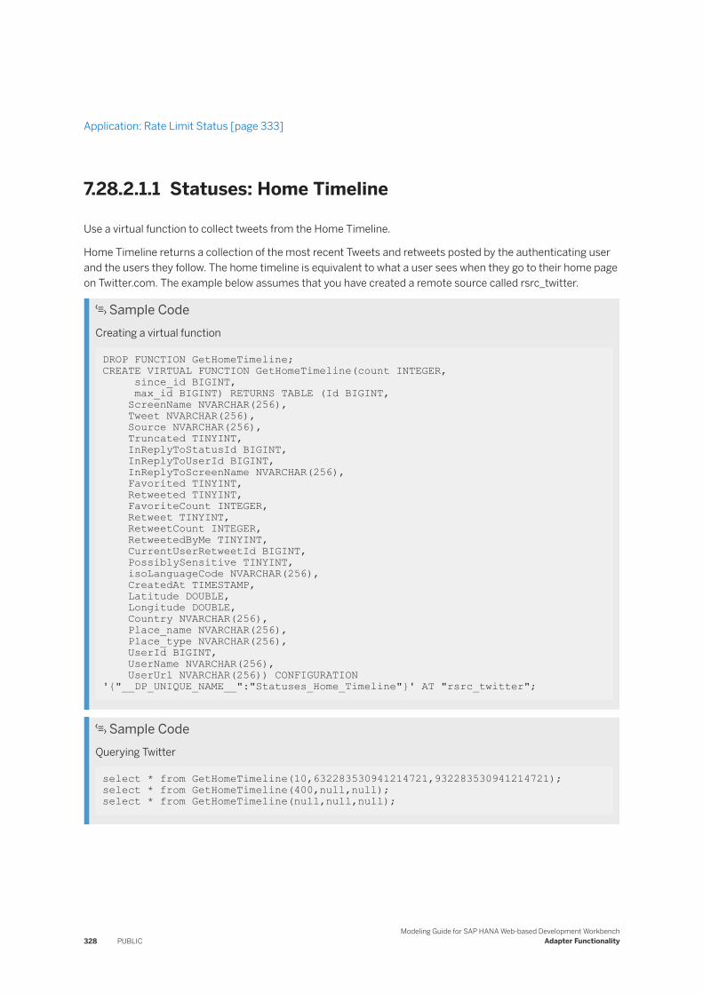
Application: Rate Limit Status [page 333]
7.28.2.1.1 Statuses: Home Timeline
Use a virtual function to collect tweets from the Home Timeline.
Home Timeline returns a collection of the most recent Tweets and retweets posted by the authenticating user and the users they follow. The home timeline is equivalent to what a user sees when they go to their home page on Twitter.com. The example below assumes that you have created a remote source called rsrc_twitter.
Sample CodeCreating a virtual function
DROP FUNCTION GetHomeTimeline; CREATE VIRTUAL FUNCTION GetHomeTimeline(count INTEGER, since_id BIGINT, max_id BIGINT) RETURNS TABLE (Id BIGINT, ScreenName NVARCHAR(256), Tweet NVARCHAR(256), Source NVARCHAR(256), Truncated TINYINT, InReplyToStatusId BIGINT, InReplyToUserId BIGINT, InReplyToScreenName NVARCHAR(256), Favorited TINYINT, Retweeted TINYINT, FavoriteCount INTEGER, Retweet TINYINT, RetweetCount INTEGER, RetweetedByMe TINYINT, CurrentUserRetweetId BIGINT, PossiblySensitive TINYINT, isoLanguageCode NVARCHAR(256), CreatedAt TIMESTAMP, Latitude DOUBLE, Longitude DOUBLE, Country NVARCHAR(256), Place_name NVARCHAR(256), Place_type NVARCHAR(256), UserId BIGINT, UserName NVARCHAR(256), UserUrl NVARCHAR(256)) CONFIGURATION '{"__DP_UNIQUE_NAME__":"Statuses_Home_Timeline"}' AT "rsrc_twitter";
Sample CodeQuerying Twitter
select * from GetHomeTimeline(10,632283530941214721,932283530941214721); select * from GetHomeTimeline(400,null,null); select * from GetHomeTimeline(null,null,null);
328 PUBLICModeling Guide for SAP HANA Web-based Development Workbench
Adapter Functionality
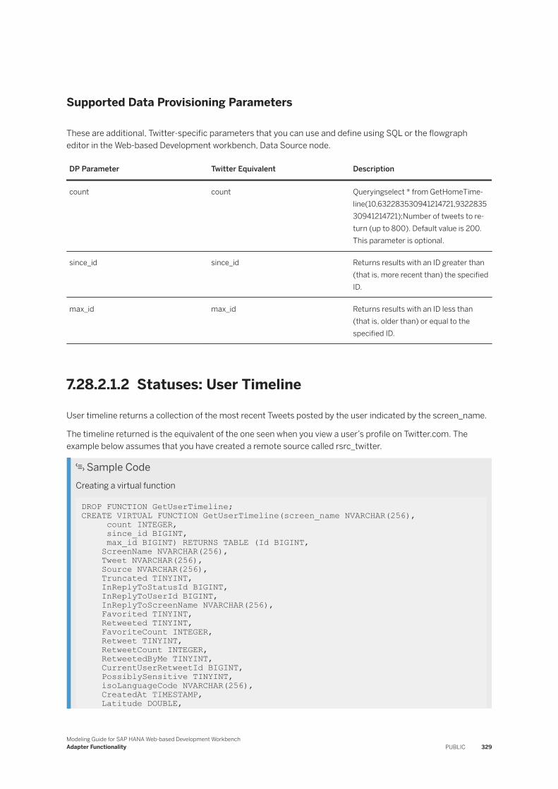
Supported Data Provisioning Parameters
These are additional, Twitter-specific parameters that you can use and define using SQL or the flowgraph editor in the Web-based Development workbench, Data Source node.
DP Parameter Twitter Equivalent Description
count count Queryingselect * from GetHomeTimeline(10,632283530941214721,932283530941214721);Number of tweets to return (up to 800). Default value is 200. This parameter is optional.
since_id since_id Returns results with an ID greater than (that is, more recent than) the specified ID.
max_id max_id Returns results with an ID less than (that is, older than) or equal to the specified ID.
7.28.2.1.2 Statuses: User Timeline
User timeline returns a collection of the most recent Tweets posted by the user indicated by the screen_name.
The timeline returned is the equivalent of the one seen when you view a user’s profile on Twitter.com. The example below assumes that you have created a remote source called rsrc_twitter.
Sample CodeCreating a virtual function
DROP FUNCTION GetUserTimeline; CREATE VIRTUAL FUNCTION GetUserTimeline(screen_name NVARCHAR(256), count INTEGER, since_id BIGINT, max_id BIGINT) RETURNS TABLE (Id BIGINT, ScreenName NVARCHAR(256), Tweet NVARCHAR(256), Source NVARCHAR(256), Truncated TINYINT, InReplyToStatusId BIGINT, InReplyToUserId BIGINT, InReplyToScreenName NVARCHAR(256), Favorited TINYINT, Retweeted TINYINT, FavoriteCount INTEGER, Retweet TINYINT, RetweetCount INTEGER, RetweetedByMe TINYINT, CurrentUserRetweetId BIGINT, PossiblySensitive TINYINT, isoLanguageCode NVARCHAR(256), CreatedAt TIMESTAMP, Latitude DOUBLE,
Modeling Guide for SAP HANA Web-based Development WorkbenchAdapter Functionality PUBLIC 329
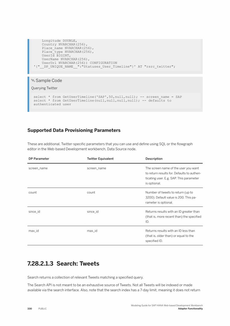
Longitude DOUBLE, Country NVARCHAR(256), Place_name NVARCHAR(256), Place_type NVARCHAR(256), UserId BIGINT, UserName NVARCHAR(256), UserUrl NVARCHAR(256)) CONFIGURATION '{"__DP_UNIQUE_NAME__":"Statuses_User_Timeline"}' AT "rsrc_twitter";
Sample CodeQuerying Twitter
select * from GetUserTimeline('SAP',50,null,null); -- screen_name = SAP select * from GetUserTimeline(null,null,null,null); -- defaults to authenticated user
Supported Data Provisioning Parameters
These are additional, Twitter-specific parameters that you can use and define using SQL or the flowgraph editor in the Web-based Development workbench, Data Source node.
DP Parameter Twitter Equivalent Description
screen_name screen_name The screen name of the user you want to return results for. Defaults to authenticating user. E.g. SAP. This parameter is optional.
count count Number of tweets to return (up to 3200). Default value is 200. This parameter is optional.
since_id since_id Returns results with an ID greater than (that is, more recent than) the specified ID.
max_id max_id Returns results with an ID less than (that is, older than) or equal to the specified ID.
7.28.2.1.3 Search: Tweets
Search returns a collection of relevant Tweets matching a specified query.
The Search API is not meant to be an exhaustive source of Tweets. Not all Tweets will be indexed or made available via the search interface. Also, note that the search index has a 7-day limit, meaning it does not return
330 PUBLICModeling Guide for SAP HANA Web-based Development Workbench
Adapter Functionality

any results older than one week. The example below assumes that you have created a remote source called rsrc_twitter.
Example
Sample CodeCreating a virtual function.
DROP FUNCTION GetSearchTweets; CREATE VIRTUAL FUNCTION GetSearchTweets(query NVARCHAR(512), count INTEGER, since_id BIGINT, max_id BIGINT, geocode NVARCHAR(256), lang ALPHANUM(2), locale ALPHANUM(2), result_type ALPHANUM(64), until DATE) RETURNS TABLE (Id BIGINT, ScreenName NVARCHAR(256), Tweet NVARCHAR(256), Source NVARCHAR(256), Truncated TINYINT, InReplyToStatusId BIGINT, InReplyToUserId BIGINT, InReplyToScreenName NVARCHAR(256), Favorited TINYINT, Retweeted TINYINT, FavoriteCount INTEGER, Retweet TINYINT, RetweetCount INTEGER, RetweetedByMe TINYINT, CurrentUserRetweetId BIGINT, PossiblySensitive TINYINT, isoLanguageCode NVARCHAR(256), CreatedAt TIMESTAMP, Latitude DOUBLE, Longitude DOUBLE, Country NVARCHAR(256), Place_name NVARCHAR(256), Place_type NVARCHAR(256), UserId BIGINT, UserName NVARCHAR(256), UserUrl NVARCHAR(256)) CONFIGURATION '{"__DP_UNIQUE_NAME__":"Search_Tweets"}' AT "rsrc_twitter" ;
Sample CodeQuerying Twitter
select * from GetSearchTweets('SAP HANA',20,643480345531273216,643484387561066497,'37.781157,-122.398720,1000mi','de','jp','recent','2015-09-15');
The previous example just shows how to use all parameters and may not return any results. To see results, specify meaningful search parameters. For example:
Modeling Guide for SAP HANA Web-based Development WorkbenchAdapter Functionality PUBLIC 331
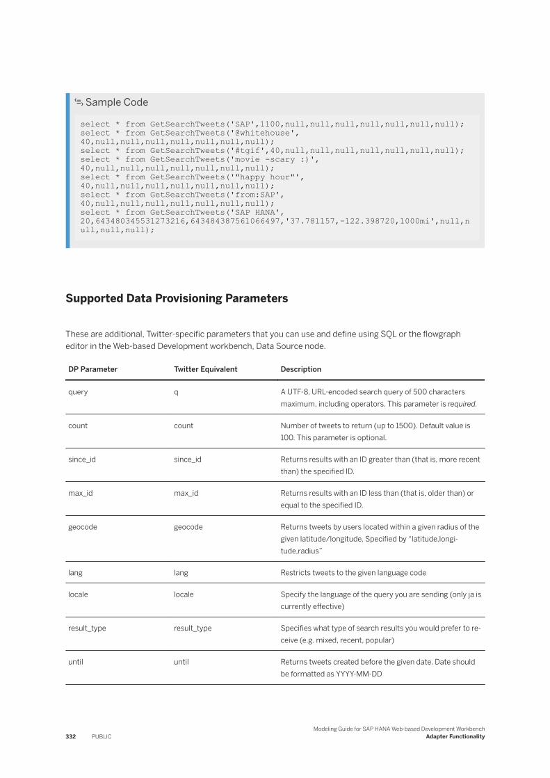
Sample Code
select * from GetSearchTweets('SAP',1100,null,null,null,null,null,null,null); select * from GetSearchTweets('@whitehouse',40,null,null,null,null,null,null,null);select * from GetSearchTweets('#tgif',40,null,null,null,null,null,null,null);select * from GetSearchTweets('movie -scary :)',40,null,null,null,null,null,null,null);select * from GetSearchTweets('"happy hour"',40,null,null,null,null,null,null,null);select * from GetSearchTweets('from:SAP',40,null,null,null,null,null,null,null);select * from GetSearchTweets('SAP HANA',20,643480345531273216,643484387561066497,'37.781157,-122.398720,1000mi',null,null,null,null);
Supported Data Provisioning Parameters
These are additional, Twitter-specific parameters that you can use and define using SQL or the flowgraph editor in the Web-based Development workbench, Data Source node.
DP Parameter Twitter Equivalent Description
query q A UTF-8, URL-encoded search query of 500 characters maximum, including operators. This parameter is required.
count count Number of tweets to return (up to 1500). Default value is 100. This parameter is optional.
since_id since_id Returns results with an ID greater than (that is, more recent than) the specified ID.
max_id max_id Returns results with an ID less than (that is, older than) or equal to the specified ID.
geocode geocode Returns tweets by users located within a given radius of the given latitude/longitude. Specified by “latitude,longitude,radius”
lang lang Restricts tweets to the given language code
locale locale Specify the language of the query you are sending (only ja is currently effective)
result_type result_type Specifies what type of search results you would prefer to receive (e.g. mixed, recent, popular)
until until Returns tweets created before the given date. Date should be formatted as YYYY-MM-DD
332 PUBLICModeling Guide for SAP HANA Web-based Development Workbench
Adapter Functionality
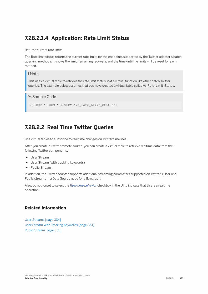
7.28.2.1.4 Application: Rate Limit Status
Returns current rate limits.
The Rate limit status returns the current rate limits for the endpoints supported by the Twitter adapter’s batch querying methods. It shows the limit, remaining requests, and the time until the limits will be reset for each method.
NoteThis uses a virtual table to retrieve the rate limit status, not a virtual function like other batch Twitter queries. The example below assumes that you have created a virtual table called vt_Rate_Limit_Status.
Sample Code
SELECT * FROM "SYSTEM"."vt_Rate_Limit_Status";
7.28.2.2 Real Time Twitter Queries
Use virtual tables to subscribe to real time changes on Twitter timelines.
After you create a Twitter remote source, you can create a virtual table to retrieve realtime data from the following Twitter components:
● User Stream● User Stream (with tracking keywords)● Public Stream
In addition, the Twitter adapter supports additional streaming parameters supported on Twitter’s User and Public streams in a Data Source node for a flowgraph.
Also, do not forget to select the Real-time behavior checkbox in the UI to indicate that this is a realtime operation.
Related Information
User Streams [page 334]User Stream With Tracking Keywords [page 334]Public Stream [page 335]
Modeling Guide for SAP HANA Web-based Development WorkbenchAdapter Functionality PUBLIC 333
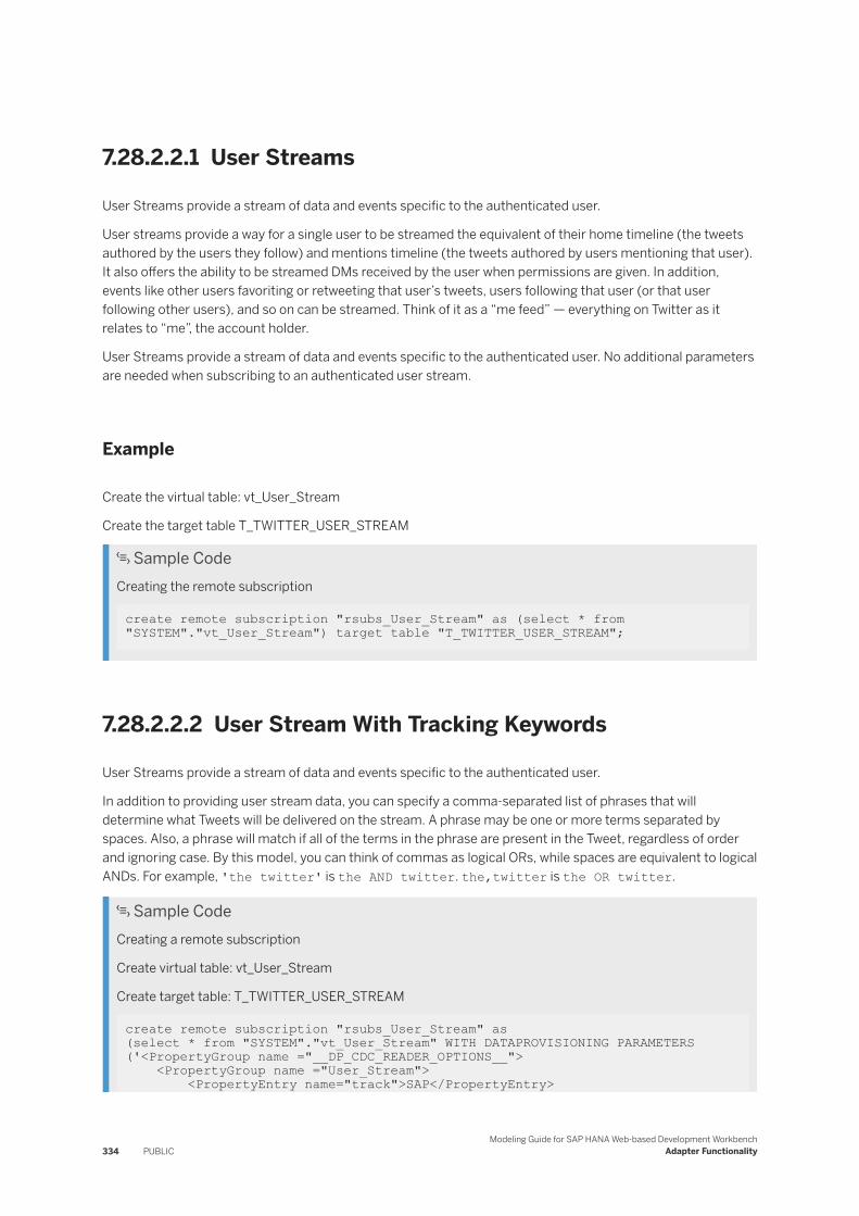
7.28.2.2.1 User Streams
User Streams provide a stream of data and events specific to the authenticated user.
User streams provide a way for a single user to be streamed the equivalent of their home timeline (the tweets authored by the users they follow) and mentions timeline (the tweets authored by users mentioning that user). It also offers the ability to be streamed DMs received by the user when permissions are given. In addition, events like other users favoriting or retweeting that user’s tweets, users following that user (or that user following other users), and so on can be streamed. Think of it as a “me feed” — everything on Twitter as it relates to “me”, the account holder.
User Streams provide a stream of data and events specific to the authenticated user. No additional parameters are needed when subscribing to an authenticated user stream.
Example
Create the virtual table: vt_User_Stream
Create the target table T_TWITTER_USER_STREAM
Sample CodeCreating the remote subscription
create remote subscription "rsubs_User_Stream" as (select * from "SYSTEM"."vt_User_Stream") target table "T_TWITTER_USER_STREAM";
7.28.2.2.2 User Stream With Tracking Keywords
User Streams provide a stream of data and events specific to the authenticated user.
In addition to providing user stream data, you can specify a comma-separated list of phrases that will determine what Tweets will be delivered on the stream. A phrase may be one or more terms separated by spaces. Also, a phrase will match if all of the terms in the phrase are present in the Tweet, regardless of order and ignoring case. By this model, you can think of commas as logical ORs, while spaces are equivalent to logical ANDs. For example, 'the twitter' is the AND twitter. the,twitter is the OR twitter.
Sample CodeCreating a remote subscription
Create virtual table: vt_User_Stream
Create target table: T_TWITTER_USER_STREAM
create remote subscription "rsubs_User_Stream" as (select * from "SYSTEM"."vt_User_Stream" WITH DATAPROVISIONING PARAMETERS ('<PropertyGroup name ="__DP_CDC_READER_OPTIONS__"> <PropertyGroup name ="User_Stream"> <PropertyEntry name="track">SAP</PropertyEntry>
334 PUBLICModeling Guide for SAP HANA Web-based Development Workbench
Adapter Functionality
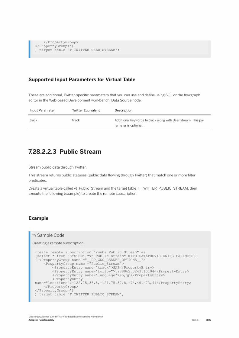
</PropertyGroup></PropertyGroup>') ) target table "T_TWITTER_USER_STREAM";
Supported Input Parameters for Virtual Table
These are additional, Twitter-specific parameters that you can use and define using SQL or the flowgraph editor in the Web-based Development workbench, Data Source node.
Input Parameter Twitter Equivalent Description
track track Additional keywords to track along with User stream. This parameter is optional.
7.28.2.2.3 Public Stream
Stream public data through Twitter.
This stream returns public statuses (public data flowing through Twitter) that match one or more filter predicates.
Create a virtual table called vt_Public_Stream and the target table T_TWITTER_PUBLIC_STREAM, then execute the following (example) to create the remote subscription.
Example
Sample CodeCreating a remote subscription
create remote subscription "rsubs_Public_Stream" as (select * from "SYSTEM"."vt_Public_Stream" WITH DATAPROVISIONING PARAMETERS ('<PropertyGroup name ="__DP_CDC_READER_OPTIONS__"> <PropertyGroup name ="Public_Stream"> <PropertyEntry name="track">SAP</PropertyEntry> <PropertyEntry name="follow">5988062,3243510104</PropertyEntry> <PropertyEntry name="language">en,jp</PropertyEntry> <PropertyEntry name="locations">-122.75,36.8,-121.75,37.8,-74,40,-73,41</PropertyEntry> </PropertyGroup></PropertyGroup>')) target table "T_TWITTER_PUBLIC_STREAM";
Modeling Guide for SAP HANA Web-based Development WorkbenchAdapter Functionality PUBLIC 335
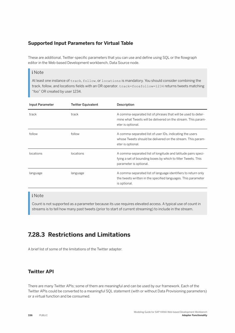
Supported Input Parameters for Virtual Table
These are additional, Twitter-specific parameters that you can use and define using SQL or the flowgraph editor in the Web-based Development workbench, Data Source node.
NoteAt least one instance of track, follow, or locations is mandatory. You should consider combining the track, follow, and locations fields with an OR operator. track=foo&follow=1234 returns tweets matching “foo” OR created by user 1234.
Input Parameter Twitter Equivalent Description
track track A comma-separated list of phrases that will be used to determine what Tweets will be delivered on the stream. This parameter is optional.
follow follow A comma-separated list of user IDs, indicating the users whose Tweets should be delivered on the stream. This parameter is optional.
locations locations A comma-separated list of longitude and latitude pairs specifying a set of bounding boxes by which to filter Tweets. This parameter is optional.
language language A comma-separated list of language identifiers to return only the tweets written in the specified languages. This parameter is optional.
NoteCount is not supported as a parameter because its use requires elevated access. A typical use of count in streams is to tell how many past tweets (prior to start of current streaming) to include in the stream.
7.28.3 Restrictions and Limitations
A brief list of some of the limitations of the Twitter adapter.
Twitter API
There are many Twitter APIs; some of them are meaningful and can be used by our framework. Each of the Twitter APIs could be converted to a meaningful SQL statement (with or without Data Provisioning parameters) or a virtual function and be consumed.
336 PUBLICModeling Guide for SAP HANA Web-based Development Workbench
Adapter Functionality

Currently, the adapter covers only few APIs, and it is very limited as to the APIs provided by Twitter. Site streams are not supported by the Twitter adapter. Site streams is an expansion of the user stream concept for services that want to stream the equivalent of “me feed” on behalf of many users at one time.
Modeling Guide for SAP HANA Web-based Development WorkbenchAdapter Functionality PUBLIC 337
8 About SAP HANA Enterprise Semantic Services
What is Enterprise Semantic Services and what can it do for my applications?
The growing volume of data in many enterprises has made it harder to leverage tasks such as:
● Get a global view of data● Find specific content● Understand where a given dataset comes from● Make use of the data for business decisions
For example, a business user wants to analyze insurance claims and is looking for an analytical model that fits her needs. She has access to hundreds of SAP HANA views that involve insurance claims, but which ones should she use? SAP HANA Enterprise Semantic Services prevents her from having to browse through numerous views and documentation and simply do a semantic search for the most relevant view.
Another example might be a business analyst who wants to acquire data from a remote system to create an SAP HANA view with vendor information. He also wants to make the view easily findable by others. He can use SAP HANA Enterprise Semantic Services search functionality to find the most relevant remote objects to acquire and publish that dataset to a knowledge graph so it is available to others. This facilitates the retrieval of remote data without having to create unnecessary additional virtual tables.
Specifically, SAP HANA Enterprise Semantic Services includes services that provide:
● Search: Enable semantic searches for objects such as tables and views. The semantic search service enables applications to submit natural language keyword search queries and combines SAP HANA linguistic text search capabilities with the semantics contained in the knowledge graph to retrieve the datasets that are most relevant to the query.
● Profiling: When acquiring a dataset, Enterprise Semantic Services profiles the data to determine the content type (also known as business type) of each column in a table (for example, ADDRESS or COUNTRY). This content type identification service automatically and interactively identifies the content types associated with the columns of any user-provided dataset (for example a Microsoft Excel file uploaded to SAP HANA).
● Publishing: An SAP HANA administrator or an application that uses the Enterprise Semantic Services API publishes a user-defined dataset to extract its semantics to the knowledge graph, which makes the dataset available for semantic search, data lineage, and join services, for example.
● Object-level data lineage: Enterprise Semantic Services provides several table functions that let you get data lineage information about SAP HANA catalog objects consisting of SAP HANA column views and activated SQL views.
NoteNot all applications that use Enterprise Semantic Services employ all of these services.
338 PUBLICModeling Guide for SAP HANA Web-based Development Workbench
About SAP HANA Enterprise Semantic Services

Related Information
Enterprise Semantic Services Knowledge Graph and Publication Requests [page 339]Search [page 340]Browsing Remote Objects in the Knowlege Graph Using a SQL View [page 348]Getting Data Lineage for Specific SAP HANA Catalog Objects [page 349]
8.1 Enterprise Semantic Services Knowledge Graph and Publication Requests
Enterprise Semantic Services enables searching and profiling datasets.
Enterprise Semantic Services uses a knowledge graph that describes the semantics of the datasets that are available to users or applications connected to SAP HANA. It is natively stored in the SAP HANA database.
Datasets represented in the knowledge graph can include tables, SQL views, SAP HANA views, remote objects in remote sources, and virtual tables that refer to remote objects.
An Enterprise Semantic Services publication request extracts information from a resource and publishes it in the knowledge graph. When a user searches for an object based on its metadata and contents, the knowledge graph provides the results.
The knowledge graph becomes populated by one or more of the following methods:
● An SAP HANA administrator uses the Enterprise Semantic Services Administration tool to publish datasets
● An SAP HANA administrator configures the Enterprise Semantic Services REST API so that an application can publish datasets
● If an application has already been configured to call the Enterprise Semantic Services REST API, the application can populate the knowledge graph. For example in SAP HANA Agile Data Preparation, when you add a worksheet, the content publishes to the knowledge graph.
Related Information
Enabling Enterprise Semantic ServicesManaging Enterprise Semantic ServicesSAP HANA Enterprise Semantic Services JavaScript API ReferenceSAP HANA Enterprise Semantic Services REST API Reference
Modeling Guide for SAP HANA Web-based Development WorkbenchAbout SAP HANA Enterprise Semantic Services PUBLIC 339

8.2 Search
Concepts and syntax for using the search functionality of SAP HANA Enterprise Semantic Services.
Related Information
Basic Search Query Syntax [page 340]Search String Examples [page 341]Search String Attribute Type and Content Type Names [page 343]Define Term Mappings for Search [page 344]Attribute Filter Expressions [page 345]
Enterprise Semantic Services REST APIEnterprise Semantic Services JavaScript API Reference
8.2.1 Basic Search Query Syntax
Basic search query syntax supported by Enterprise Semantic Services.
query ::= [ scope-spec ] ( qualified-expression )+
scope-spec ::= (' category ' | ' appscope ' ) ' : ' IDENTIFIER ( scope-spec ) ?
qualified-expression ::= [ ' + ' | ' - ' ] term-expression
term-expression ::= attribute-type-expression | attribute-filter-expression | term
attribute-type-expression ::= (attribute-type-name ' :: ' ( disjunctive-term-expression | conjunctive-term-expression | term )) | ' date ' ' :: ' (disjunctive-date-expression | conjunctive-date-expression | date)
attribute-filter-expression ::= attribute-filter-name ' : ' ( disjunctive-term-expression | conjunctive-term-expression | term )
disjunctive-term-expression ::= ' ( ' term ( ' OR ' term )* ' ) '
conjunctive-term-expression ::= ' ( ' term ( ' AND ' term )* ' ) '
disjunctive-date-expression ::= ' ( ' date ( ' OR ' date )* ' ) '
conjunctive-date-expression ::= ' ( ' date ( ' AND ' date )* ' ) '
term ::= WORD | PHRASE
attribute-name ::= IDENTIFIER
attribute-type-name ::= 'AddressLine' | 'FullAddress' | 'BuildingName' | 'StreetName' | 'SecondaryAddress' | 'Country' | 'City' | 'Postcode' | 'Region' | 'Firm' | 'Person' | 'FirstName' | 'LastName' | 'HonoraryPostname' | 'MaturityPostname' | 'Prename' | 'PersonOrFirm' | 'Title' | 'Phone' | 'SSN' | 'NameInitial' | 'Email' /* attribute type names are case-insensitive */
340 PUBLICModeling Guide for SAP HANA Web-based Development Workbench
About SAP HANA Enterprise Semantic Services
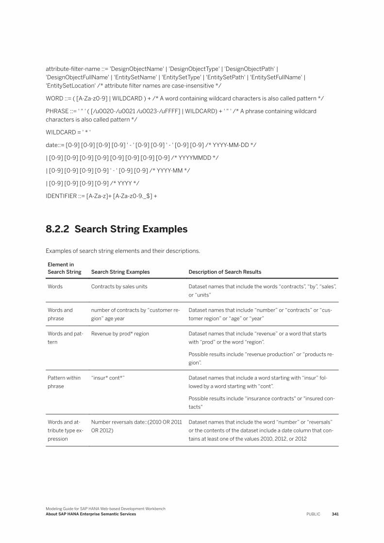
attribute-filter-name ::= 'DesignObjectName' | 'DesignObjectType' | 'DesignObjectPath' | 'DesignObjectFullName' | 'EntitySetName' | 'EntitySetType' | 'EntitySetPath' | 'EntitySetFullName' | 'EntitySetLocation' /* attribute filter names are case-insensitive */
WORD ::= ( [A-Za-z0-9] | WILDCARD ) + /* A word containing wildcard characters is also called pattern */
PHRASE ::= ' " ' ( [/u0020-/u0021 /u0023-/uFFFF] | WILDCARD) + ' " ' /* A phrase containing wildcard characters is also called pattern */
WILDCARD = ' * '
date::= [0-9] [0-9] [0-9] [0-9] ' - ' [0-9] [0-9] ' - ' [0-9] [0-9] /* YYYY-MM-DD */
| [0-9] [0-9] [0-9] [0-9] [0-9] [0-9] [0-9] [0-9] /* YYYYMMDD */
| [0-9] [0-9] [0-9] [0-9] ' - ' [0-9] [0-9] /* YYYY-MM */
| [0-9] [0-9] [0-9] [0-9] /* YYYY */
IDENTIFIER ::= [A-Za-z]+ [A-Za-z0-9._$] +
8.2.2 Search String Examples
Examples of search string elements and their descriptions.
Element in Search String Search String Examples Description of Search Results
Words Contracts by sales units Dataset names that include the words “contracts”, “by”, “sales”, or “units”
Words and phrase
number of contracts by “customer region” age year
Dataset names that include “number” or “contracts” or “customer region” or “age” or “year”
Words and pattern
Revenue by prod* region Dataset names that include “revenue” or a word that starts with “prod” or the word “region”.
Possible results include “revenue production” or “products region”.
Pattern within phrase
“insur* cont*” Dataset names that include a word starting with “insur” followed by a word starting with “cont”.
Possible results include “insurance contracts" or "insured contacts"
Words and attribute type expression
Number reversals date::(2010 OR 2011 OR 2012)
Dataset names that include the word “number” or “reversals” or the contents of the dataset include a date column that contains at least one of the values 2010, 2012, or 2012
Modeling Guide for SAP HANA Web-based Development WorkbenchAbout SAP HANA Enterprise Semantic Services PUBLIC 341

Element in Search String Search String Examples Description of Search Results
Words and qualified expression
Loss and Expense +"Outstanding Reserves"
Loss and Expense -insurance
Dataset names that optionally include the word “loss” or “expense”, but must contain "outstanding reserves"
Dataset names that optionally include “loss” or “expense”, but must not contain "insurance"
Date values Date::2000
Date::(2000 AND 2001-01 AND 2001-02-01)
Date::(2000 OR 2001-01 OR 2001-02-01)
Dataset that contains a date column with the value 2000.
Dataset that contains a date column with the value 2000 and 2001-01 and 2001-02-01.
Dataset that contains a date column with the value 2000 or 2001-01 or 2001-02-01.
Attribute type expressions with geography values
city::("New York" OR Paris)
country::(USA AND Canada)
region::"Ile de France"
Dataset that contains a city column with either the value “New York” or “Paris”
Dataset that contains a country column with both the value “USA” and “Canada”
Dataset that contains a region column with the value “Ile de France”
Attribute type expressions with pattern
City::Washington*
LastName::Panla*
Dataset that contains a city column with a value that starts with “Washington”
Dataset that contains a last name column with a value that starts with “Panla”
Attribute filter expressions
EntitySetLocation:local foodmart
EntitySetFullName:(foodmart OR adventureworks)
EntitySetType:table
DesignObjectType:"hana * view"
Entitysets matching “foodmart” in local SAP HANA instance
Entitysets with their name matching either “foodmart” or “adventureworks”
Entitysets of sql table or hana virtual table type
Entitysets with design objects of hana calculation view, hana attribute view, or hana analytic view type
See Attribute Filter Expressions [page 345].
Note● Stopwords are either ignored or considered optional in a phrase. Stopwords are any pronoun,
preposition, conjunction, particle, determiner, and auxiliary.For example, “number of contracts” will include the search results “number contracts” and “number of contracts”.
● Special characters are ignored. Special characters include \/;,.:-_()[]<>!?*@+{}="&.For example, “contract_number” will be handled as “contract number”.
342 PUBLICModeling Guide for SAP HANA Web-based Development Workbench
About SAP HANA Enterprise Semantic Services

8.2.3 Search String Attribute Type and Content Type Names
The search string can contain an attribute type name that corresponds to a content type name.
The search results will return data set names that contain the content type and specified value.
NoteAttribute type names are not case sensitive in search strings.
Attribute Type in Search String Content Type Name
AddressLine Address Line
FullAddress Full Address
BuildingName Building Name
StreetName Street Name
SecondaryAddress Secondary Address
Country Country
City City
Postcode Postcode
Region Region
Firm Firm
Person Person
FirstName First Name
LastName Last Name
HonoraryPostname Honorary Postname
MaturityPostname Maturity Postname
Prename Prename
PersonOrFirm Person Or Firm
Title Title
Date Date
Phone Phone
SSN SSN
NameInitial Name Initial
Modeling Guide for SAP HANA Web-based Development WorkbenchAbout SAP HANA Enterprise Semantic Services PUBLIC 343
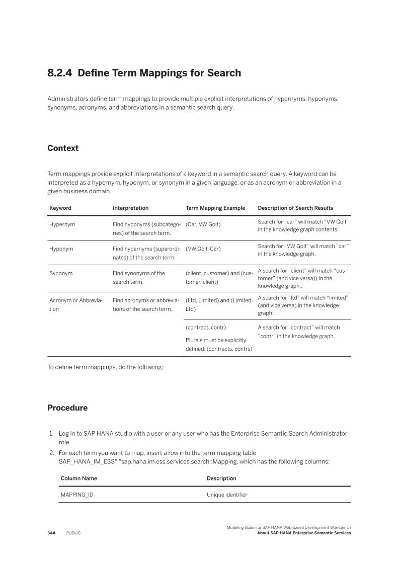
8.2.4 Define Term Mappings for Search
Administrators define term mappings to provide multiple explicit interpretations of hypernyms, hyponyms, synonyms, acronyms, and abbreviations in a semantic search query.
Context
Term mappings provide explicit interpretations of a keyword in a semantic search query. A keyword can be interpreted as a hypernym, hyponym, or synonym in a given language, or as an acronym or abbreviation in a given business domain.
Keyword Interpretation Term Mapping Example Description of Search Results
Hypernym Find hyponyms (subcategories) of the search term.
(Car, VW Golf) Search for “car” will match “VW Golf" in the knowledge graph contents.
Hyponym Find hypernyms (superordinates) of the search term.
(VW Golf, Car) Search for “VW Golf” will match “car” in the knowledge graph.
Synonym Find synonyms of the search term.
(client, customer) and (customer, client)
A search for “client” will match “customer” (and vice versa)) in the knowledge graph..
Acronym or Abbreviation
Find acronyms or abbreviations of the search term.
(Ltd, Limited) and (Limited, Ltd)
A search for “ltd” will match “limited” (and vice versa) in the knowledge graph.
(contract, contr)
Plurals must be explicitly defined: (contracts, contrs)
A search for “contract” will match “contr” in the knowledge graph.
To define term mappings, do the following:
Procedure
1. Log in to SAP HANA studio with a user or any user who has the Enterprise Semantic Search Administrator role.
2. For each term you want to map, insert a row into the term mapping table SAP_HANA_IM_ESS"."sap.hana.im.ess.services.search::Mapping, which has the following columns:
Column Name Description
MAPPING_ID Unique identifier
344 PUBLICModeling Guide for SAP HANA Web-based Development Workbench
About SAP HANA Enterprise Semantic Services
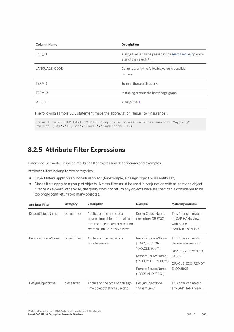
Column Name Description
LIST_ID A list_id value can be passed in the search.request parameter of the search API.
LANGUAGE_CODE Currently, only the following value is possible:○ en
TERM_1 Term in the search query.
TERM_2 Matching term in the knowledge graph.
WEIGHT Always use 1.
The following sample SQL statement maps the abbreviation “Insur” to “insurance”.
insert into "SAP_HANA_IM_ESS"."sap.hana.im.ess.services.search::Mapping" values ('20','1','en','Insur','insurance',1);
8.2.5 Attribute Filter Expressions
Enterprise Semantic Services attribute filter expression descriptions and examples.
Attribute filters belong to two categories:
● Object filters apply on an individual object (for example, a design object or an entity set)● Class filters apply to a group of objects. A class filter must be used in conjunction with at least one object
filter or a keyword; otherwise, the query does not return any objects because the filter is considered to be too broad (can return too many objects).
Attribute Filter Category Description Example Matching example
DesignObjectName object filter Applies on the name of a design-time object from which runtime objects are created; for example, an SAP HANA view.
DesignObjectName: (inventory OR ECC)
This filter can match an SAP HANA view with name INVENTORY or ECC.
RemoteSourceName object filter Applies on the name of a remote source.
RemoteSourceName: ("DB2_ECC" OR "ORACLE ECC")
RemoteSourceName: ("*ECC*" OR "*ECC*")
RemoteSourceName: ("DB2" AND "ECC")
This filter can match the remote sources:
DB2_ECC_REMOTE_SOURCE
ORACLE_ECC_REMOTE_SOURCE
DesignObjectType class filter Applies on the type of a design-time object that was used to
DesignObjectType: "hana * view"
This filter can match any SAP HANA view.
Modeling Guide for SAP HANA Web-based Development WorkbenchAbout SAP HANA Enterprise Semantic Services PUBLIC 345
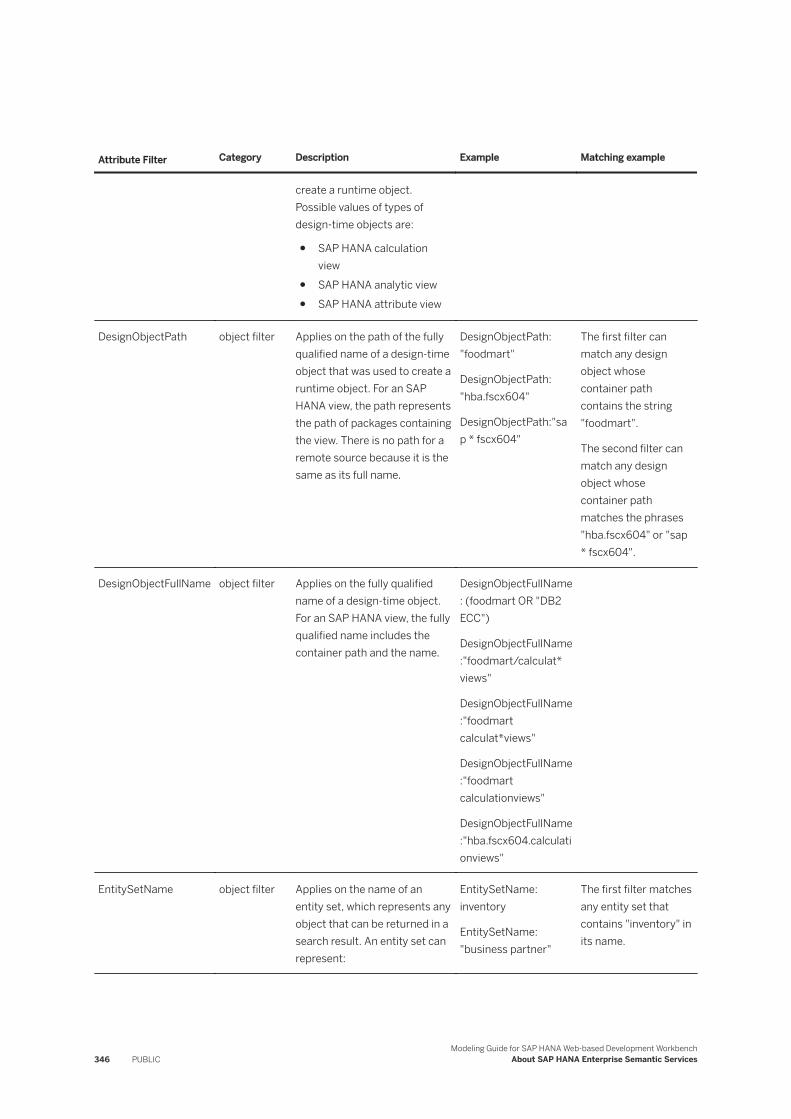
Attribute Filter Category Description Example Matching example
create a runtime object. Possible values of types of design-time objects are:
● SAP HANA calculation view
● SAP HANA analytic view● SAP HANA attribute view
DesignObjectPath object filter Applies on the path of the fully qualified name of a design-time object that was used to create a runtime object. For an SAP HANA view, the path represents the path of packages containing the view. There is no path for a remote source because it is the same as its full name.
DesignObjectPath: "foodmart"
DesignObjectPath: "hba.fscx604"
DesignObjectPath:"sap * fscx604"
The first filter can match any design object whose container path contains the string "foodmart".
The second filter can match any design object whose container path matches the phrases "hba.fscx604" or "sap * fscx604".
DesignObjectFullName object filter Applies on the fully qualified name of a design-time object. For an SAP HANA view, the fully qualified name includes the container path and the name.
DesignObjectFullName: (foodmart OR "DB2 ECC")
DesignObjectFullName:"foodmart/calculat* views"
DesignObjectFullName:"foodmart calculat*views"
DesignObjectFullName:"foodmart calculationviews"
DesignObjectFullName:"hba.fscx604.calculationviews"
EntitySetName object filter Applies on the name of an entity set, which represents any object that can be returned in a search result. An entity set can represent:
EntitySetName: inventory
EntitySetName: "business partner"
The first filter matches any entity set that contains "inventory" in its name.
346 PUBLICModeling Guide for SAP HANA Web-based Development Workbench
About SAP HANA Enterprise Semantic Services
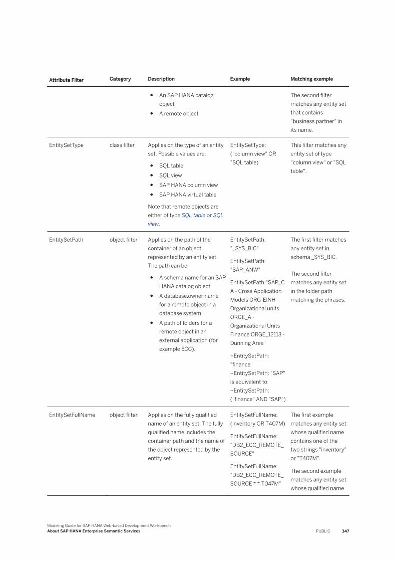
Attribute Filter Category Description Example Matching example
● An SAP HANA catalog object
● A remote object
The second filter matches any entity set that contains "business partner" in its name.
EntitySetType class filter Applies on the type of an entity set. Possible values are:
● SQL table● SQL view● SAP HANA column view● SAP HANA virtual table
Note that remote objects are either of type SQL table or SQL view.
EntitySetType: ("column view" OR "SQL table)"
This filter matches any entity set of type "column view" or "SQL table".
EntitySetPath object filter Applies on the path of the container of an object represented by an entity set. The path can be:
● A schema name for an SAP HANA catalog object
● A database.owner name for a remote object in a database system
● A path of folders for a remote object in an external application (for example ECC).
EntitySetPath: "_SYS_BIC"
EntitySetPath: "SAP_ANW"
EntitySetPath:"SAP_CA - Cross Application Models ORG-EINH - Organizational units ORGE_A - Organizational Units Finance ORGE_12113 - Dunning Area"
+EntitySetPath: "finance" +EntitySetPath: "SAP" is equivalent to: +EntitySetPath: ("finance" AND "SAP")
The first filter matches any entity set in schema _SYS_BIC.
The second filter matches any entity set in the folder path matching the phrases.
EntitySetFullName object filter Applies on the fully qualified name of an entity set. The fully qualified name includes the container path and the name of the object represented by the entity set.
EntitySetFullName: (inventory OR T407M)
EntitySetFullName: "DB2_ECC_REMOTE_SOURCE"
EntitySetFullName: "DB2_ECC_REMOTE_SOURCE * * T047M"
The first example matches any entity set whose qualified name contains one of the two strings "inventory" or "T407M".
The second example matches any entity set whose qualified name
Modeling Guide for SAP HANA Web-based Development WorkbenchAbout SAP HANA Enterprise Semantic Services PUBLIC 347
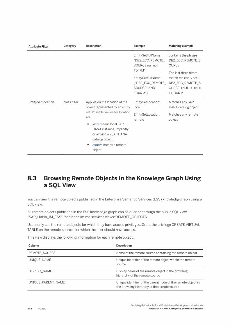
Attribute Filter Category Description Example Matching example
EntitySetFullName: "DB2_ECC_REMOTE_SOURCE null null T047M"
EntitySetFullName: ("DB2_ECC_REMOTE_SOURCE" AND "T047M")
contains the phrase DB2_ECC_REMOTE_SOURCE.
The last three filters match the entity set: DB2_ECC_REMOTE_SOURCE.<NULL>.<NULL>.T047M
EntitySetLocation class filter Applies on the location of the object represented by an entity set. Possible values for location are:
● local means local SAP HANA instance, implicitly qualifying an SAP HANA catalog object
● remote means a remote object
EntitySetLocation: local
EntitySetLocation: remote
Matches any SAP HANA catalog object
Matches any remote object
8.3 Browsing Remote Objects in the Knowlege Graph Using a SQL View
You can view the remote objects published in the Enterprise Semantic Services (ESS) knowledge graph using a SQL view.
All remote objects published in the ESS knowledge graph can be queried through the public SQL view "SAP_HANA_IM_ESS"."sap.hana.im.ess.services.views::REMOTE_OBJECTS".
Users only see the remote objects for which they have access privileges. Grant the privilege CREATE VIRTUAL TABLE on the remote sources for which the user should have access.
This view displays the following information for each remote object.
Column Description
REMOTE_SOURCE Name of the remote source containing the remote object
UNIQUE_NAME Unique identifier of the remote object within the remote source
DISPLAY_NAME Display name of the remote object in the browsing hierarchy of the remote source
UNIQUE_PARENT_NAME Unique identifier of the parent node of the remote object in the browsing hierarchy of the remote source
348 PUBLICModeling Guide for SAP HANA Web-based Development Workbench
About SAP HANA Enterprise Semantic Services
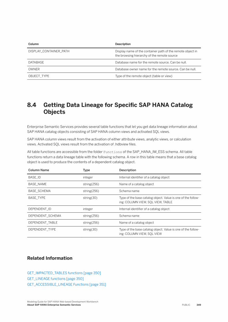
Column Description
DISPLAY_CONTAINER_PATH Display name of the container path of the remote object in the browsing hierarchy of the remote source
DATABASE Database name for the remote source. Can be null.
OWNER Database owner name for the remote source. Can be null.
OBJECT_TYPE Type of the remote object (table or view)
8.4 Getting Data Lineage for Specific SAP HANA Catalog Objects
Enterprise Semantic Services provides several table functions that let you get data lineage information about SAP HANA catalog objects consisting of SAP HANA column views and activated SQL views.
SAP HANA column views result from the activation of either attribute views, analytic views, or calculation views. Activated SQL views result from the activation of .hdbview files.
All table functions are accessible from the folder Functions of the SAP_HANA_IM_ESS schema. All table functions return a data lineage table with the following schema. A row in this table means that a base catalog object is used to produce the contents of a dependent catalog object.
Column Name Type Description
BASE_ID integer Internal identifier of a catalog object
BASE_NAME string(256) Name of a catalog object
BASE_SCHEMA string(256) Schema name
BASE_TYPE string(30) Type of the base catalog object. Value is one of the following: COLUMN VIEW, SQL VIEW, TABLE
DEPENDENT_ID integer Internal identifier of a catalog object
DEPENDENT_SCHEMA string(256) Schema name
DEPENDENT_TABLE string(256) Name of a catalog object
DEPENDENT_TYPE string(30) Type of the base catalog object. Value is one of the following: COLUMN VIEW, SQL VIEW
Related Information
GET_IMPACTED_TABLES functions [page 350]GET_LINEAGE functions [page 350]GET_ACCESSIBLE_LINEAGE Functions [page 351]
Modeling Guide for SAP HANA Web-based Development WorkbenchAbout SAP HANA Enterprise Semantic Services PUBLIC 349

8.4.1 GET_IMPACTED_TABLES functions
GET_IMPACTED_TABLES functions return an instance of the data lineage table with specific properties.
The properties are as follows:
● A row in the table represents a direct or indirect data lineage relationship between a BASE object and a DEPENDENT object.
● BASE_TYPE is only equal to 'TABLE'.● DEPENDENT_TYPE can be one of: 'SYNONYM', 'COLUMN VIEW', or 'SQL VIEW'. The synonym is defined
on a SQL view or an SAP HANA view.
The functions are as follows:
● "SAP_HANA_IM_ESS"."sap.hana.im.ess.services.views.datalineage::GET_ALL_IMPACTING_TABLES" takes no argument and returns all tables used directly or indirectly to produce every SAP HANA column view or activated SQL view.
● "SAP_HANA_IM_ESS"."sap.hana.im.ess.services.views.datalineage::GET_IMPACTING_TABLES" returns all tables used directly or indirectly to produce the catalog object passed as parameter to the function. There are two parameters:
SCHEMA_NAME NVARCHAR(256) VIEW_NAME NVARCHAR(256)
These functions are accessible with ROLE: sap.hana.im.ess.roles::DataSteward.
8.4.2 GET_LINEAGE functions
GET_LINEAGE functions return an instance of the data lineage table with specific properties.
The properties are as follows:
● Each row in the returned table represents a direct data lineage relationship between a BASE object and a DEPENDENT object.
● BASE_TYPE can be one of: 'TABLE', 'PROCEDURE', 'FUNCTION', 'SYNONYM', 'COLUMN VIEW', or 'SQL VIEW'.
● DEPENDENT_TYPE can be one of: 'PROCEDURE', 'FUNCTION', 'SYNONYM', 'COLUMN VIEW', or 'SQL VIEW'.
The functions are as follows:
● "SAP_HANA_IM_ESS"."sap.hana.im.ess.services.views.datalineage::GET_LINEAGE_FROM_SCHEMA" takes a schema name as input and returns all objects (tables or views) used directly or indirectly to produce every SAP HANA column view or activated SQL view contained in the input schema. The input parameter is:
SCHEMA_NAME NVARCHAR(256)
● "SAP_HANA_IM_ESS"."sap.hana.im.ess.services.views.datalineage::GET_LINEAGE_FROM_VIEW" takes a view name from a schema name as input and returns all objects (tables or views) used directly or indirectly
350 PUBLICModeling Guide for SAP HANA Web-based Development Workbench
About SAP HANA Enterprise Semantic Services
to produce every SAP HANA column view or activated SQL view contained in the input view. The input parameters are:
SCHEMA_NAME NVARCHAR(256) VIEW_NAME NVARCHAR(256)
These functions are accessible with ROLE: sap.hana.im.ess.roles::DataSteward.
8.4.3 GET_ACCESSIBLE_LINEAGE Functions
GET_ACCESSIBLE_LINEAGE functions return an instance of the data lineage table with specific properties.
For a connected user with the name user, the properties are:
● Each row in the returned table represents either:○ A direct data lineage relationship between a BASE object V1 and a DEPENDENT object V2 when user
has been granted a SELECT privilege on both V1 and V2.○ An indirect data lineage relationship between a BASE object V1 and a DEPENDENT object V2 when V1
is indirectly used to produce V2, user has been granted a SELECT privilege on both V1 and V2, and there is no intermediate object between V1 and V2 on which user is granted SELECT privilege.
● BASE_TYPE can be one of: 'TABLE', 'PROCEDURE', 'FUNCTION', 'SYNONYM', 'COLUMN VIEW', or 'SQL VIEW'.
● DEPENDENT_TYPE can be one of: 'PROCEDURE', 'FUNCTION', 'SYNONYM', 'COLUMN VIEW', or 'SQL VIEW'.
The functions are as follows:
● "SAP_HANA_IM_ESS"."sap.hana.im.ess.services.views.datalineage::GET_ACCESSIBLE_LINEAGE_FROM_SCHEMA" takes a schema name as input and returns all objects (tables or views) used directly or indirectly to produce every SAP HANA column view or activated SQL view contained in the input schema. The input parameter is:
SCHEMA_NAME NVARCHAR(256)
● "SAP_HANA_IM_ESS"."sap.hana.im.ess.services.views.datalineage::GET_ACCESSIBLE_LINEAGE_FROM_VIEW" takes a view name from a schema name as input and returns all objects (tables or views) used directly or indirectly to produce every SAP HANA column view or activated SQL view contained in the input view. The input parameters are:
SCHEMA_NAME NVARCHAR(256) VIEW_NAME NVARCHAR(256)
These functions are accessible with ROLE: sap.hana.im.ess.roles::User.
Modeling Guide for SAP HANA Web-based Development WorkbenchAbout SAP HANA Enterprise Semantic Services PUBLIC 351
Important Disclaimers and Legal Information
HyperlinksSome links are classified by an icon and/or a mouseover text. These links provide additional information.About the icons:
● Links with the icon : You are entering a Web site that is not hosted by SAP. By using such links, you agree (unless expressly stated otherwise in your agreements with SAP) to this:
● The content of the linked-to site is not SAP documentation. You may not infer any product claims against SAP based on this information.● SAP does not agree or disagree with the content on the linked-to site, nor does SAP warrant the availability and correctness. SAP shall not be liable for any
damages caused by the use of such content unless damages have been caused by SAP's gross negligence or willful misconduct.
● Links with the icon : You are leaving the documentation for that particular SAP product or service and are entering a SAP-hosted Web site. By using such links, you agree that (unless expressly stated otherwise in your agreements with SAP) you may not infer any product claims against SAP based on this information.
Videos Hosted on External PlatformsSome videos may point to third-party video hosting platforms. SAP cannot guarantee the future availability of videos stored on these platforms. Furthermore, any advertisements or other content hosted on these platforms (for example, suggested videos or by navigating to other videos hosted on the same site), are not within the control or responsibility of SAP.
Beta and Other Experimental FeaturesExperimental features are not part of the officially delivered scope that SAP guarantees for future releases. This means that experimental features may be changed by SAP at any time for any reason without notice. Experimental features are not for productive use. You may not demonstrate, test, examine, evaluate or otherwise use the experimental features in a live operating environment or with data that has not been sufficiently backed up.The purpose of experimental features is to get feedback early on, allowing customers and partners to influence the future product accordingly. By providing your feedback (e.g. in the SAP Community), you accept that intellectual property rights of the contributions or derivative works shall remain the exclusive property of SAP.
Example CodeAny software coding and/or code snippets are examples. They are not for productive use. The example code is only intended to better explain and visualize the syntax and phrasing rules. SAP does not warrant the correctness and completeness of the example code. SAP shall not be liable for errors or damages caused by the use of example code unless damages have been caused by SAP's gross negligence or willful misconduct.
Bias-Free LanguageSAP supports a culture of diversity and inclusion. Whenever possible, we use unbiased language in our documentation to refer to people of all cultures, ethnicities, genders, and abilities.
352 PUBLICModeling Guide for SAP HANA Web-based Development Workbench
Important Disclaimers and Legal Information

Modeling Guide for SAP HANA Web-based Development WorkbenchImportant Disclaimers and Legal Information PUBLIC 353
www.sap.com/contactsap
© 2021 SAP SE or an SAP affiliate company. All rights reserved.
No part of this publication may be reproduced or transmitted in any form or for any purpose without the express permission of SAP SE or an SAP affiliate company. The information contained herein may be changed without prior notice.
Some software products marketed by SAP SE and its distributors contain proprietary software components of other software vendors. National product specifications may vary.
These materials are provided by SAP SE or an SAP affiliate company for informational purposes only, without representation or warranty of any kind, and SAP or its affiliated companies shall not be liable for errors or omissions with respect to the materials. The only warranties for SAP or SAP affiliate company products and services are those that are set forth in the express warranty statements accompanying such products and services, if any. Nothing herein should be construed as constituting an additional warranty.
SAP and other SAP products and services mentioned herein as well as their respective logos are trademarks or registered trademarks of SAP SE (or an SAP affiliate company) in Germany and other countries. All other product and service names mentioned are the trademarks of their respective companies.
Please see https://www.sap.com/about/legal/trademark.html for additional trademark information and notices.
THE BEST RUN