
Hunt Scanlon Select Guide to America's Leading Executive Recruiters
Upload
khangminh22Category
view
3download
0
Effects of grid resolution in a three-dimensional hydrostatic model:
Modeling field observations
by
Joshua Allen Scanlon
A thesis submitted to the graduate faculty
in partial fulfillment of the requirements for the degree of
MASTER OF SCIENCE
Major: Civil Engineering (Environmental Engineering)
Program of Study Committee:
Chris Rehmann, Major Professor
Timothy Ellis
John Downing
Iowa State University
Ames, Iowa
2010
Copyright © Joshua Allen Scanlon, 2010. All rights reserved.

ii
This thesis is dedicated to my parents, who have always challenged me to
succeed in all of life’s endeavors. I would not be where I am today without
your love and support.

iii
TABLE OF CONTENTS
LIST OF TABLES v
LIST OF FIGURES vi
ACKNOWLEDGEMENTS ix
ABSTRACT x
NOTATION LIST xi
CHAPTER 1: INTRODUCTION 1
Significance 1
Objectives 4
Hypotheses 4
Organization 5
CHAPTER 2: BACKGROUND AND LITERATURE REVIEW 6
Introduction 6
Stratification 6
Internal Waves and Seiches 8
Dimensionless Numbers 14
Rossby Number 14
Richardson Number 16
Wedderburn Number 18
Lake Number 19
Degeneration of Internal Waves 21
Lake Modeling 24
Governing Equations 24
Analytical Models 27
One-Layer 28
Two-Layer 31
N-Layer 37
Numerical Models 40
Hydrostatic Models 41
Applications of Numerical Models 44
Effects of Grid Resolution in Numerical Models 47
Non-Hydrostatic Models 52
Examples and Applications of Non-Hydrostatic Models 52
Summary 54
CHAPTER 3: METHODOLOGY 56
Introduction 56
iv
Field Work 57
Ada Hayden Lake 57
West Okoboji Lake 59
Lake Diagnostic System 61
Thermistor Chains 62
Estuary, Lake, and Coastal Ocean Model 65
Bathymetry 66
Pre-Processing 73
Temperature Profiles 74
Environmental Forcing 77
Designating Model Output, Running Simulation, and Post-Processing 78
Description of Numerical Methods 79
Momentum Discretization 80
Scalar Transport 83
Mixing Model 84
Data Analysis of Field Work and Model Results 85
Normalized Potential Energy 87
Normalized Kinetic Energy 89
Willmott Skill Number 91
Summary 92
CHAPTER 4: RESULTS AND DISCUSSION 94
Introduction 94
Field Results 94
Ada Hayden Lake 95
West Okoboji Lake 102
Simulation Events and Results 108
Simulation 1: High Lake Number 109
Simulation 2: Moderate Lake Number 129
Simulation 3: Low Lake Number 146
Combining Simulation Results 161
Validation of Hydrostatic Assumption 168
Summary 172
CHAPTER 5: CONCLUSIONS 174
Summary 174
Recommendations 176
Future Work 178
APPENDIX 180
REFERENCES 192

v
LIST OF TABLES
Table 2.1. Matrix values for conservation equation coefficients 39
Table 3.1. Keywords used in ELCOM files 70
Table 3.2. ELCOM files 71
Table 4.1. Summary of simulation events 109
Table 4.2. ELCOM resolutions for Simulation 1 model runs 111
Table 4.3. ELCOM resolutions for Simulation 2 model runs 130
Table 4.4. ELCOM resolutions for Simulation 3 model runs 148
Table 4.5. Scaling parameters 162
Table 4.6. Parameters used to estimate steepening timescale 169
vi
LIST OF FIGURES
Figure 2.1. Typical temperature structure of stratified lakes 7
Figure 2.2. Schematic view of various seiche modes 11
Figure 2.3. Regime boundaries for degeneration mechanisms 23
Figure 2.4. Definition sketch for a two-layer model 32
Figure 3.1. Bathymetric map of Ada Hayden Lake 58
Figure 3.2. Bathymetric map of West Okoboji Lake 60
Figure 3.3. ELCOM grid for Ada Hayden Lake 67
Figure 4.1. Field results from Ada Hayden Lake in 2007 96
Figure 4.2. Field results from Ada Hayden Lake in 2008 97
Figure 4.3. Change in stratification in Ada Hayden Lake 99
Figure 4.4. Internal wave degeneration regimes for Ada Hayden Lake 101
Figure 4.5. Field results from West Okoboji Lake in 2009 103
Figure 4.6. Histogram of NL values 104
Figure 4.7. Changes in stratification in West Okoboji Lake 105
Figure 4.8. Internal wave degeneration regimes for West Okoboji Lake 107
Figure 4.9. Profiles for Ada Hayden Lake 110
Figure 4.10. Time series temperature profiles from Simulation 1 112
measured from the LDS using x 15 m, z 0.1 m
Figure 4.11. Time series temperature profiles from Simulation 1 113
measured from T-Chain 52 using x 15 m, z 0.1 m
Figure 4.12. Time series temperature profiles from Simulation 1 115
measured from the LDS using x 15 m, z 0.6 m
Figure 4.13. Time series temperature profiles from Simulation 1 116
measured from T-Chain 52 using x 15 m, z 0.6 m
Figure 4.14. The effect of NL on numerical error during Simulation 1 118
Figure 4.15. PE from Simulation 1 measured by the LDS 119
Figure 4.16. PE from Simulation 1 measured by T-Chain 52 120

vii
Figure 4.17. KE from Simulation 1 measured by the LDS 122
Figure 4.18. KE from Simulation 1 measured by T-Chain 52 123
Figure 4.19. Displacement power spectra from Ada Hayden Lake 124
Figure 4.20. Spectral density of the 17°C isotherm during Simulation 1 125
Figure 4.21. Observed and modeled isotherm depth for Simulation 1 127
Figure 4.22. WS from Simulation 1 128
Figure 4.23. Time series temperature profiles from Simulation 2 132
measured from the LDS using x 10 m, z 0.1 m
Figure 4.24. Time series temperature profiles from Simulation 2 133
measured from T-Chain 52 using x 10 m, z 0.1 m
Figure 4.25. Time series temperature profiles from Simulation 2 134
measured from T-Chain 53 using x 10 m, z 0.1 m
Figure 4.26. The effect of NL on numerical error during Simulation 2 136
Figure 4.27. PE from Simulation 2 measured by the LDS 137
Figure 4.28. PE from Simulation 2 measured by T-Chain 52 138
Figure 4.29. PE from Simulation 2 measured by T-Chain 53 139
Figure 4.30. KE from Simulation 1 measured by the LDS 140
Figure 4.31. KE from Simulation 1 measured by T-Chain 52 141
Figure 4.32. KE from Simulation 1 measured by T-Chain 53 142
Figure 4.33. Spectral density of the 17°C isotherm during Simulation 2 143
Figure 4.34. Observed and modeled isotherm depth for Simulation 2 144
Figure 4.35. WS from Simulation 2 145
Figure 4.36. Profiles for West Okoboji Lake 147
Figure 4.37. Time series temperature profiles from Simulation 3 149
measured from the LDS using x 50 m, z 1 m
Figure 4.38. Time series temperature profiles from Simulation 3 150
measured from T-Chain 52 using x 50 m, z 1 m
viii
Figure 4.39. The effect of NL on numerical error during Simulation 3 153
Figure 4.40. PE from Simulation 3 measured by the LDS 153
Figure 4.41. PE from Simulation 3 measured by T-Chain 52 154
Figure 4.42. KE from Simulation 3 measured by the LDS 155
Figure 4.43. KE from Simulation 3 measured by T-Chain 52 156
Figure 4.44. Spectral density of the 18.5°C isotherm during Simulation 3 157
Figure 4.45. Observed and modeled isotherm depth from Simulation 3 158
Figure 4.46. WS from Simulation 3 160
Figure 4.47. Combined normalized energy results from Simulation 1 163
Figure 4.48. Combined normalized energy results from Simulation 2 164
Figure 4.49. Combined normalized energy results from Simulation 3 165
Figure 4.50. Combined normalized energy results from Simulations 1 and 3 167
Figure 4.51. Γ values for simulations 168
Figure 4.52. Time to steepening 170

ix
ACKNOWLEDGEMENTS
I would first like to then the National Science Foundation Physical Oceanography
Program for their financial support of this project. To Danielle Wain, thank you for all
the help you gave in paving the way for my contribution to this project. For all your help
over the last two years, I‘d like to thank Mike Kohn. Although it‘s quite possible that
we‘ve spent entirely too much time out on the lake with each other, I couldn‘t imagine a
better friend to do it with all over again. For all their help with the field work, I‘d like to
thank Adam Wright, Emily Libbey, and Taryn Tigges. I‘d like to acknowledge Peter van
der Linden, Matt Fairchild, Jane Shuttleworth, and Dennis Heimdal at Iowa Lakeside
Laboratory; you never stopped to amaze me with your willingness to assist with our field
work, allowing us access to lab space, and the genuine interest you gave in our research.
I‘d like to thank Gary Owen at the Iowa Department of Natural Resources and Tom Clary
at Clary Lake Service, for their help with the logistics of the 2009 field study. To my
office mate Joel Sikkema, thanks for all the friendly debates, lunch-hour chats, and being
a soundboard for my ideas. I would also like to thank my committee, Drs. Tim Ellis and
John Downing. Finally, I‘d like to extend my gratitude to my advisor Dr. Chris Rehmann
for your guidance, support, and advice; your enthusiasm for science is truly inspiring.
I would be remiss if I didn‘t thank my wife Kadera. As always, thank you for the
patience and love you constantly exhibit.
x
ABSTRACT
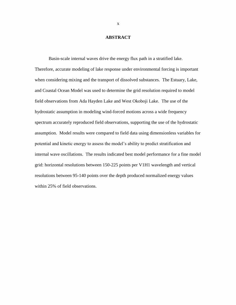
Basin-scale internal waves drive the energy flux path in a stratified lake.
Therefore, accurate modeling of lake response under environmental forcing is important
when considering mixing and the transport of dissolved substances. The Estuary, Lake,
and Coastal Ocean Model was used to determine the grid resolution required to model
field observations from Ada Hayden Lake and West Okoboji Lake. The use of the
hydrostatic assumption in modeling wind-forced motions across a wide frequency
spectrum accurately reproduced field observations, supporting the use of the hydrostatic
assumption. Model results were compared to field data using dimensionless variables for
potential and kinetic energy to assess the model‘s ability to predict stratification and
internal wave oscillations. The results indicated best model performance for a fine model
grid: horizontal resolutions between 150-225 points per V1H1 wavelength and vertical
resolutions between 95-140 points over the depth produced normalized energy values
within 25% of field observations.
xi
NOTATION LIST
A = area
ijA = matrix coefficients for conservation of momentum
sA = surface area
ka = viscous discretization term for top face of cell k
ma = eigenvector for the m
th vertical mode
1A = integration constant in normal mode equation
B = basin width
ijB = matrix coefficients for continuity
kb = viscous discretization term for cell k
C = baroclinic discretization operator in ELCOM
DC = drag coefficient
CFL = Courant-Friedrichs-Lewy number
kc = viscous discretization term for bottom face of cell k
mc = wave phase speed for the mth
vertical mode
nc = wave phase speed
,x yD = horizontal diffusion operators in the x and y-direction, respectively
BE = background potential energy
DE = dynamic energy
KE = kinetic energy per unit area
KE = normalized kinetic energy
PE = potential energy per unit area
,0PE = potential energy reference value
,fieldPE = potential energy calculated using field data

xii
,modelPE = potential energy calculated using model data
PE = normalized potential energy
mF = modal forcing function for the mth
vertical mode
Fr = Froude number
f = Coriolis frequency
G = explicit source term in ELCOM
g = gravitational acceleration
g = reduced gravity
H = total undisturbed water depth
h = effective water depth
ih = thickness of the ith
layer
I = advective discretization operator in ELCOM
i = cell location in the x-direction
j = cell location in the y-direction
K = shear velocity constant
K = wavenumber vector
k = cell location in the z-direction
Kk = x-component of the wavenumber
L = basin length
NL = Lake number
RL = Rossby radius
Kl = y-component of the wavenumber
M = mixing operator in ELCOM
Km = z-component of the wavenumber
N = buoyancy frequency
n = time
xn = number of horizontal nodes
xiii
zn = number of vertical nodes
p = pressure
mQ = modal transport due to the mth
vertical mode
0R = Rossby number
bRi = bulk Richardson number
gRi = gradient Richardson number
S = scalar value in ELCOM
( )CS = scalar source in ELCOM
*S = scalar concentration due to advection in ELCOM
S = scalar concentration after mixing in ELCOM
tS = Schmidt stability
wS = water surface
T = wave period
bT = bore timescale
dT = damping timescale
iT = wave period of the ith
vertical mode
KHT = billowing timescale
sT = steepening timescale
wT = wind duration
U = matrix containing u velocities at grid locations specified in ELCOM
hU = depth-averaged water velocity in the x-direction
iU = depth-averaged water velocity in the x-direction in the ith
layer
u = fluid velocity vector
u = x-component of the water velocity
wu = wind speed at 10 m
*u = shear velocity

xiv
V = matrix containing v velocities at grid locations specified in ELCOM
v = y-component of the water velocity
W = Wedderburn number
WS = Willmott skill number
w = z-component of the water velocity
fieldw = vertical velocity calculated from field data
modelw = vertical velocity calculated from model data
0w = velocity amplitude
fieldX = physical parameter based on field observations
fieldX = time-averaged parameter value from field observations
modelX = physical parameter based on model results
z = elevation
sz = elevation of the water surface
tz = elevation of the center of the metalimnion
vz = elevation of the center of volume
0z = elevation of lake bottom
1z = elevation of the bottom of the metalimnion
2z = elevation of the top of the metalimnion
= coefficient of the nonlinear term in the wave equation
m = eigenvalue for the mth
vertical mode
= numerical error scaling parameter
C = critical value of the numerical error scaling parameter
k = boundary condition variable in ELCOM
PE = fluctuations in potential energy calculated from model data
Z = vector of vertical grid size in ELCOM
x = horizontal grid size
t = model time step

xv
z = vertical grid size
= density jump across an interface
t = sub model time step
,x y = discrete difference operators in x or y-direction, respectively
0 = metalimnion thickness
= wave displacement
e = end wall vertical displacement
i = displacement of the ith
layer
s = surface displacement
0 = initial wave displacement
= free surface height
= angle wavenumber makes to horizontal
= diffusivity
vK = von Kármán‘s constant
= numerical diffusivity in a diffusion-dominated system
= numerical diffusivity in a dissipation-dominated system
= wavelength of the V1H1 internal wave
0 = initial wavelength of the gravest mode
= dynamic viscosity of water
= kinematic viscosity of water
= numerical viscosity in a diffusion-dominated system
= numerical viscosity in a dissipation-dominated system
3 = viscosity in the z-direction
m = modal pressure due to the mth
vertical mode
= water density
a = air density

xvi
i = ith
layer water density
0 = reference density
= density perturbation from reference value
= background density
b = shear at lake bottom
s = timescale to the onset of steepening
0 = wind-applied surface shear
= mode shape
= latitude
= dimensionless parameter for numerical error terms
= Earth‘s angular velocity
= wave frequency
D Dt = mt c x , substantial derivative of
1
CHAPTER 1: INTRODUCTION
Significance
The structure and hydrodynamics of lakes are important when considering the
transport of dissolved substances and overall water quality. The presence of water
constituents such as oxygen, nutrients, micro-organisms, and plankton play a large role in
water quality in lakes and reservoirs. Stratification—typically caused by temperature,
salinity, or both—restricts vertical mixing and therefore plays a large role in water
column variability, such as affecting the availability of nutrients to phytoplankton
(MacIntyre et al., 1999). For temperate freshwater lakes at mid-latitudes, stratification
depends on temperature and the season. Two turnover periods in the spring and autumn
vertically mix the lake throughout, with a period of strong stratification during the
summer months. During the summer, the thermal structure of the lake consists of a well
mixed surface layer (epilmnion), a quiescent weakly stratified bottom layer
(hypolimnion), and a region of rapid density change (metalimnion, or thermocline) which
separates the top and bottom layers.
Imberger (1998) outlined the energy flux path in a stratified lake by separating the
overall flux into four processes: i) momentum transfer due to wind-applied surface shear,
ii) seiching of internal waves, which can be related to the magnitude of the Wedderburn
or Lake numbers, iii) degeneration of waves into higher frequency motions such as
solitons, supercritical bores, and shear instabilities, and iv) damping of internal motions
which leads to the thickening of the benthic boundary layer. The basin-scale energy flux
2
from the wind is of particular interest because of its dominant role in setting the
thermocline in motion, which in the absence of inflows and outflows, is the primary
energy store for transport and mixing below the wind-mixed layer. Therefore, modeling
the basin-scale internal wave behavior is a requirement to modeling and quantifying the
flux paths of nutrients in a stratified lake (Imberger, 1998). Recent evidence shows that
seiching by long-period, basin-scale waves in a stratified lake generates a turbulent
benthic boundary layer that can be many meters thick in the hypolimnion (Lemckert and
Imberger, 1998). The internal wave field was shown to have implications for the
distributions of variables such as dissolved oxygen, nitrate, hydrogen sulfide, and the
reduction-oxidation potential in the metalimnion (Eckert et al., 2002), and upwelling
conditions due to internal waves have been responsible for several fish kills (Marti-
Cardona et al., 2008).
Modeling stratified systems can therefore have implications to predict water
quality and the spatial variability of water parameters (e.g., temperature, salinity, and
dissolved oxygen), characterize lake response under certain forcing conditions, and
implement real-time water management systems. Layered models have been used to
estimate upwelling conditions (Stevens and Lawrence, 1997), predict vertical
displacements in the water column (Heaps and Ramsbottom, 1966), simulate the seasonal
deepening of the mixed layer (Spigel and Imberger, 1980), and estimate mixed layer
shear (Monismith, 1985). Three-dimensional, hydrostatic, numerical models have been
shown to accurately predict basin-scale behavior (i.e., Casulli and Cheng, 1992; Saggio
and Imberger, 1998; Hodges et al., 2000). These three-dimensional models discretize the
flows onto a model grid composed of computational cells. These cells are used to

3
represent scalar concentrations, fluid velocities, and free surface elevations. Although
hydrostatic models have been a useful tool in coastal ocean (and similar) systems, there is
the criticism of the inability of a hydrostatic model to reproduce non-hydrostatic forces.
These non-hydrostatic conditions shift the energy flux to small-scale mechanisms, such
as wave steepening, shear billowing, and supercritical bores. To resolve non-hydrostatic
forces, grid-switching strategies have been presented (Botelho et al., 2009) which result
in a hybrid hydrostatic/non-hydrostatic model. Additionally, fully non-hydrostatic
models have been shown to be successful in predicting non-linear motions (Botelho and
Imberger, 2007; Kocyigit and Falconer, 2004).
However, despite the success of three-dimensional numerical models, numerical
errors in the form of numerical diffusion and numerical viscosity can compromise model
results (Rueda et al., 2007; Hodges and Rueda, 2008). Methods have been put forth to
minimize numerical diffusion using filters (Laval et al., 2003a) or to assimilate field data
directly into the model during a simulation run (Yeates et al., 2008). Empirical formulas
relating numerical diffusivity and numerical viscosity to grid size have been found for
diffusionless, inviscid, two-dimensional, simple non-linear systems using a three-
dimensional hydrostatic model (Hodges et al., 2006). However, no work has been done
to quantify numerical error due to model resolution while modeling real world, fully
three-dimensional, wind-forced events.

4
Objectives
The goal of this work is to i) observe internal waves and forcing conditions across
a wide frequency range, ii) assess the validity of the hydrostatic assumption in modeling
observed events, iii) compare predictions from a three-dimensional, hydrostatic,
numerical model to field observations, iv) provide a dialogue which quantifies model
performance, and v) develop general guidelines for choosing grid sizes and model time
steps.
Hypotheses
Deep lakes at mid-latitutdes can be classified as temperate lakes, which are
defined to possess summer and winter stratification separated by two overturn events
(Kalf, 2002). Preliminary field data and previous literature (i.e., Fee, 1967; Fee and
Bachmann, 1968) indicate a stratified environment suitable for the formation of internal
wave activity in two Iowa lakes. Stratified conditions during the course of the summer
months are initially hypothesized to be suitable for analysis using a hydrostatic numerical
model. The ability of a numerical model to capture internal wave motions is limited by
the grid size (e.g., Schwab and Dietrich, 1997; Hodges et al. 2000; Botelho et al., 2009).
Therefore, higher model resolution should be able to better resolve internal wave
motions. Thus, it is hypothesized that the more refined the model grid, the better the
model‘s results. The model time step should be selected as to provide stable results, as
described by the Courant-Friedrichs-Lewy condition.

5
Organization
In this thesis, a background of physical limnology and a review of existing work
will be presented in Chapter 2. Chapter 3 will address the methodology pertaining to
field work, model implementation, and data analysis techniques. In Chapter 4, field and
simulation results will be presented, as well as discussion on the significance of those
results. A summary of the work, as well as recommendations for future work, will be
given in Chapter 5.
6
CHAPTER 2: BACKGROUND AND LITERATURE REVIEW
Introduction
Chapter 2 reviews the background and existing work on lake response and
hydrodynamics. An introductory discussion of hydrodynamics focuses on stratification
and internal waves. Dimensionless numbers related to physical limnology are presented
and outlined in terms of their importance for both past and present work. Analytical
solutions are presented, as well as the simplifications involved when finding solutions
which can accurately represent a wind-forced stratified system. Numerical schemes are
introduced, with a description of a particular numerical model for its use in this work.
The summary offers the motivation and significance behind the present work in context
of previous work.
Stratification
For freshwater lakes, the thermal structure often consists of a well mixed
epilimnion, a metalimnion with a steep temperature gradient, and a deeper weakly
stratified hypolimnion (Fig. 2.1). The metalimnion can be referred to as the pycnocline
when incorporating density effects on stratification, or a thermocline when considering
the effects of temperature stratification. This layering of lower density water above
higher density water is one example of stratification in nature. Generally, stratification is
gravitationally stable, and acts to inhibit motion in the vertical direction (parallel to the

7
Figure 2.1. Typical temperature structure of stratified lakes during the summer months,
with warmer water overlaying colder water.
density gradient). Therefore, motions generated within the stratified fluid tend to be
greater in the horizontal direction.
For dimictic lakes, this stratification is established through solar heating of the
surface layer during the summer months. The spring and fall overturn periods—caused
by heating and cooling of the surface waters, respectively—occur when the entire water
column reaches the same density and is mixed vertically throughout. Therefore, during
the summer months when stratification is present, inhibited vertical mixing results in
comparatively low dissolved oxygen levels in the hypolimnion. Wind further adds
energy to the lake through various mechanisms. Surface stresses generate turbulence that
Epilimnion
Metalimnion
n
Hypolimnion
Density

8
keeps the epilimnion well mixed. The wind shear also forms surface gravity waves
which add further energy when they break and convectively mix the epilimnion. Wind
stress can also tilt the water surface by pushing surface water from the windward to the
leeward side of the lake.
Internal Waves and Seiches
Waves are generated because of a restoring force that tends to bring a disturbed
system back to its original state and inertia that causes the system to overshoot the
undisturbed position (Kundu and Cohen, 2008). In the case of a density-stratified fluid,
waves can form when a horizontal density interface is disturbed. The density interface
can consist of a water-air interface such as a water surface, or a water-water surface with
lower density water overlying higher density water, in the case of stratified lakes. When
gravity acts as the restoring force, gravity waves form. Non-dispersive, small amplitude
waves will obey the wave equation
2 2 2 22
2 2 2 2nct x y z
(2.1)
where is the wave displacement and nc is the phase speed. In a fluid with a constant
density gradient, the solution for the displacement in a long rectangular basin is given by
(Gill, 1982)

9
0 cos( )K K Kk x l y m z t (2.2)
where 0 is the initial displacement (positive upwards), , ,K K Kk l mK is the
wavenumber vector, and is the wave frequency. The internal wave‘s vertical velocity
w can be calculated by taking the time derivative of the isotherm displacement. The
horizontal velocities u and v are defined in the x and y directions, respectively. To
simplify the analysis, assume two-dimensional flow, giving the solutions for u and w
0 sin K Kw w k x m z t (2.3)
0 sin K K
mu w k x m z t
k (2.4)
where 0 0w is the velocity amplitude. For two-dimensional internal waves where the
amplitudes for which the amplitudes are small compared to the wavelength, linear wave
theory gives the frequency of the wave as related to the wavenumber vector K by the
dispersion relation
1/22
2 2cosK
K K
kN N
k m
(2.5)
10
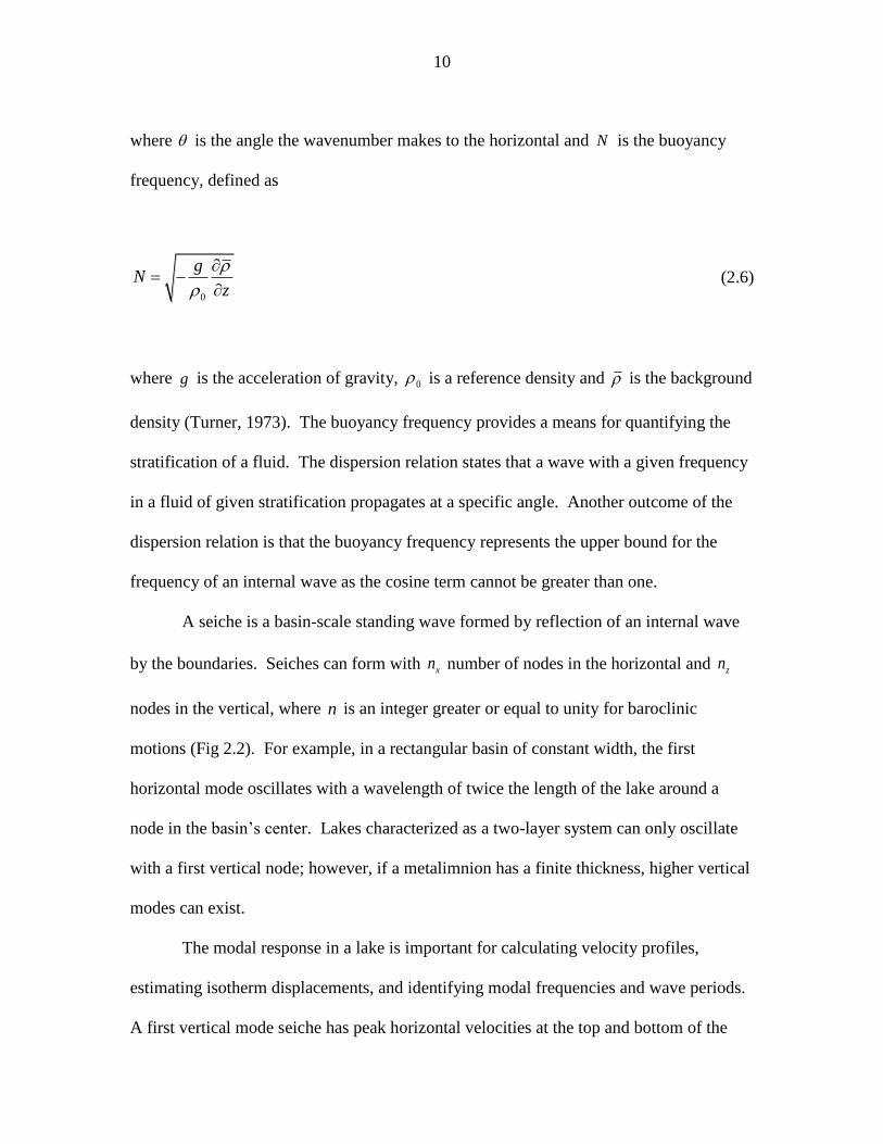
where is the angle the wavenumber makes to the horizontal and N is the buoyancy
frequency, defined as
0
gN
z
(2.6)
where g is the acceleration of gravity, 0 is a reference density and is the background
density (Turner, 1973). The buoyancy frequency provides a means for quantifying the
stratification of a fluid. The dispersion relation states that a wave with a given frequency
in a fluid of given stratification propagates at a specific angle. Another outcome of the
dispersion relation is that the buoyancy frequency represents the upper bound for the
frequency of an internal wave as the cosine term cannot be greater than one.
A seiche is a basin-scale standing wave formed by reflection of an internal wave
by the boundaries. Seiches can form with xn number of nodes in the horizontal and zn
nodes in the vertical, where n is an integer greater or equal to unity for baroclinic
motions (Fig 2.2). For example, in a rectangular basin of constant width, the first
horizontal mode oscillates with a wavelength of twice the length of the lake around a
node in the basin‘s center. Lakes characterized as a two-layer system can only oscillate
with a first vertical node; however, if a metalimnion has a finite thickness, higher vertical
modes can exist.
The modal response in a lake is important for calculating velocity profiles,
estimating isotherm displacements, and identifying modal frequencies and wave periods.
A first vertical mode seiche has peak horizontal velocities at the top and bottom of the

11
Figure 2.2. Schematic view of various seiche modes in a closed basin. Interfaces are
shown for the initial maximum displacement (solid line) and one-half period later (dashed
line).
water column, while increasing the number of vertical nodes yields more peaks in the
velocity profile. A second vertical mode experiences an expansion and compression of
the metalimnion, therefore resulting in more peaks in the velocity profile with a
maximum velocity within the metalimnion (Münnich et al., 1992). The first vertical
mode will see the highest shear at that central node, as the direction of horizontal velocity
changes. Higher vertical nodes generate shear at each node with consequently shorter
distances between these points. Therefore, higher nodes are more damped (Vidal et al.,
2005). For evaluating the normal vertical mode, the simplest case is for a continuously
stratified fluid with constant buoyancy frequency. Gill (1982) showed that the mode
shape is governed by
a) V1H1
d) V3H1 c) V2H1
b) V1H2
12
2 2
2 20
n
N
z c
(2.7)
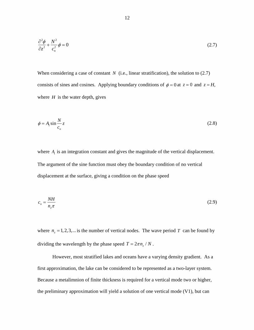
When considering a case of constant N (i.e., linear stratification), the solution to (2.7)
consists of sines and cosines. Applying boundary conditions of 0 at 0z and z H,
where H is the water depth, gives
1 sinn
NA z
c (2.8)
where 1A is an integration constant and gives the magnitude of the vertical displacement.
The argument of the sine function must obey the boundary condition of no vertical
displacement at the surface, giving a condition on the phase speed
n
z
NHc
n (2.9)
where 1,2,3,...zn is the number of vertical nodes. The wave period T can be found by
dividing the wavelength by the phase speed 2 /zT n N .
However, most stratified lakes and oceans have a varying density gradient. As a
first approximation, the lake can be considered to be represented as a two-layer system.
Because a metalimnion of finite thickness is required for a vertical mode two or higher,
the preliminary approximation will yield a solution of one vertical mode (V1), but can
13
contain multiple horizontal nodes. Turner (1973) gave the angular frequency of the
V1Hn seiche as
1 2
1 22
xn h hg
L h h
(2.10)
where xn is the number of horizontal nodes, 0/g g which is the reduced gravity at
the epilimnion-hypolimnion interface, is the density difference between the top and
bottom layers, 0 is a reference density, commonly taken as the hypolimnion density, 1h
is the thickness of the epilimnion, and 2h is the hypolimnion thickness.
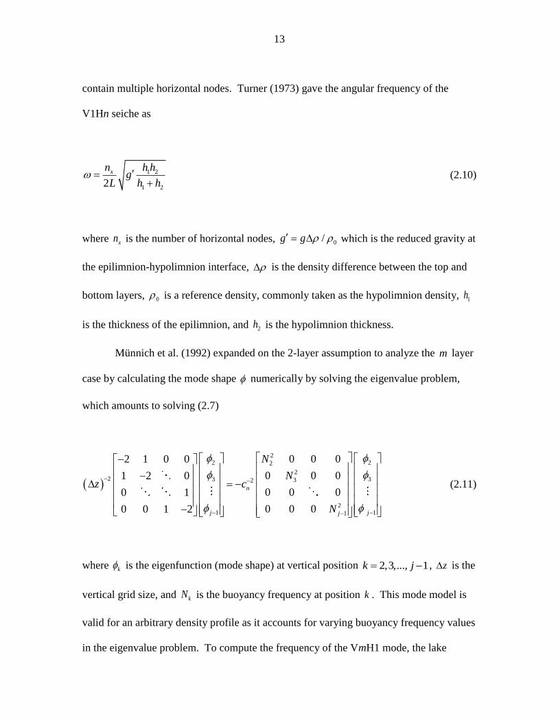
Münnich et al. (1992) expanded on the 2-layer assumption to analyze the m layer
case by calculating the mode shape numerically by solving the eigenvalue problem,
which amounts to solving (2.7)
22 22
22 3 332
21 11
0 0 02 1 0 0
0 0 01 2 0
0 0 00 1
0 0 00 0 1 2
n
j jj
N
Nz c
N
(2.11)
where k is the eigenfunction (mode shape) at vertical position 2,3,..., 1k j , z is the
vertical grid size, and kN is the buoyancy frequency at position k . This mode model is
valid for an arbitrary density profile as it accounts for varying buoyancy frequency values
in the eigenvalue problem. To compute the frequency of the VmH1 mode, the lake
14
length L is divided by the solution for nc from (2.11). For a rectangular lake, the
solution for multiple horizontal nodes is more straightforward than solving an eigenvalue
problem. The VmHn frequency is n times that of the VmH1. Correspondingly, the wave
periods for the VmH2-4 modes are half, one-third, and one-quarter that of the VmH1.
Dimensionless Numbers
Several dimensionless numbers are used in physical limnology and geophysical
fluid dynamics. The benefit of a dimensionless number lies in its use when comparing
various systems across different scales. This section will outline dimensionless numbers
as they pertain to this work.
Rossby Number
The description ―large-scale‖ varies from one system to the next. Atmospheric
flows are typical at much larger scales than oceanic flows, which in turn are of much
larger scale than a laboratory flume. In the case of geophysical fluid dynamics, motions
are to be considered large-scale when the effect of Earth‘s rotation becomes increasingly
important (Pedlosky, 1979). The relative strengths of advective and Coriolis forces are
given in the Rossby number 0R , defined as
0
uR
fB (2.12)
15
where B is the width of flow, 2 sinf is the Coriolis frequency, calculated using
as the Earth‘s angular velocity (7.3 × 10⁻⁵
s-1
) and latitude . The Coriolis frequency is
positive in the northern hemisphere and negative in the southern hemisphere. It varies
from 1.45 × 10⁻⁴
s-1
at the poles to zero at the equator. The physical meaning behind
the Coriolis frequency varying with latitude is that a person standing on a pole rotates,
while a person standing on the equator merely translates (Kundu and Cohen, 2008).
Rotation can affect internal wave as the wave‘s frequency approaches the Coriolis
frequency. Thus, a limit has been placed on both the upper and lower bounds of an
internal wave‘s frequency, such that f N . Similarly, effects of the Earth‘s rotation
can be neglected if 1oR . For low frequency waves, a length scale representing the
effect of rotation on the wavelength is given by the Rossby radius RL , defined as
1R
NhL
f (2.13)
where 1h is the thickness of the epilimnion. The Rossby radius gives the length at which
rotation forces begin to become significant. For an enclosed basin, such as a lake, the
Rossby radius can indicate whether the basin size allows for rotational effects due to
Coriolis forces. If the basin width is less than RL , rotational forces can be considered
negligible, which may apply to small lakes or water bodies with a long and narrow basin.
16
Richardson Number
Another useful relation for physical limnology and other stratified flows is the
comparison of potential to kinetic energy. In this work, the relation takes the form of the
bulk Richardson number bRi and gradient Richardson number gRi . The bulk Richardson
number is used when comparing the buoyancy force to the inertia force in a layer of fluid.
The gradient Richardson number is used for a local comparison between the velocity
gradient and stratification (or buoyancy effects) and is important when dealing with
turbulence and instability. When considering infinitesimal disturbances in a fluid with
linear density and velocity profiles, the stability criterion for the gradient Richardson
number guarantees stable flows for 1/ 4bRi (Kundu and Cohen, 2008). The Richardson
number, both in bulk and gradient form, are defined as
2
*
b
g hRi
u
(2.14)
2
2/
g
NRi
u z
(2.15)
where h is the depth of the top layer in a system with two or more layers (or the total
depth for a single layer system), while the shear velocity *u and reduced gravity g
defined as

17
0*
0
u
(2.16)
and
2 1
0
g g
(2.17)
where 0 is the wind-applied shear, 2 is the density of the bottom layer, and 1 is the
density of the top layer. However, it is difficult to directly measure shear. The shear
velocity can be estimated using measured wind speed by the following
2
*
0
a D wC uu
(2.18)
where a is the air density, DC is the drag coefficient, wu is the wind speed measured at
10 m above the water surface. In the case of a one-layer system, 2 is the density of
water, and 1 is the air density. Since the density of water is approximately 1000 times
that of air, g g . However, in a two-layer system 2 will be slightly larger than 1 ,
resulting with g O (10-2
) m/s2. Wüest and Lorke (2003) performed a least squares fit
of data from several studies to yield values for the drag coefficient based on wind speed
wu

18
1.150.0044 for 5 m/sD w wC u u (2.19)
2
2
1 10ln for 5 m/sD w
vK D w
gC K u
C u
(2.20)
where vK is von Kármán‘s constant (typically taken to be 0.41) and the constant K is
taken to be 11.3 (Smith, 1988; Yelland and Taylor, 1966). Typical values for DC range
from 0.0011 (at wu = 5 m/s) to 0.0021 (at wu = 25 m/s). Estimates of wind speed can
therefore be directly applied to estimate the applied wind shear.
Wedderburn Number
To relate the response of a lake to wind forcing, Spigel and Imberger (1980)
modeled the lake as a two-layer system and showed that the response of the upper mixed
layer depended on the magnitude of bRi for the upper layer and the aspect ratio of the
layer depth to the lake‘s length (i.e. /h L ). Thompson and Imberger (1980) combined
these two terms to form the Wedderburn number W defined as
2
1
2
*
g hW
u L
(2.21)
This classification based on W allows for a simple description of the lake
response pertaining to the interface tilt. A condition in which 1/ 2W corresponds to

19
the interface surfacing at the windward end of the lake, resulting in upwelling. Greater
stratification will result in higher Wedderburn numbers, as g increases. Alternatively,
as either wind speed increases or stratification strength decreases, W decreases,
indicating greater movement of the interface.
Lake Number
The Wedderburn number provides valuable insight into the lake response given
some basic information concerning the stratification, wind forcing, and basin size. While
these are important parameters to use for describing the lake behavior as a whole, it does
not account for the lake‘s bathymetry. To incorporate the lake bathymetry, an estimate of
the lake‘s stability tS is required:
0
sz
t vS z z A z z dz (2.22)
where sz is the height of the water surface, ( )A z and z are the area and density as a
function of depth, respectively, and vz is the center of volume of the lake, defined as
0
0
( )
( )
s
s
z
v z
zA z dzz
A z dz
(2.23)

20
A ratio of stabilizing to de-stabilizing forces may be made by taking moments about the
center of volume. This ratio will yield a dimensionless group referred to as the Lake
number NL (Imberger and Patterson, 1990)
2 3/2
0 *
1 /
1 /
t t s
N
s v s
gS z zL
u A z z
(2.24)
where sA is the area of the water surface sA z and tz is the height to the center of the
metalimnion. The stabilizing forces are defined using (2.22) coupled with gravitational
acceleration and the destabilizing forces attributed to wind stress, which were not
previously defined but are represented in the denominator of (2.24).
The Lake number is defined in a similar manner to the Wedderburn number in
that 1NL corresponds to upwelling at the windward end of the lake and 10NL will
result in no isotherm tilting; therefore, internal waves will theoretically exist for 10NL
(MacIntyre et al., 1999). For large Lake numbers, stratification will dominate the wind
shear forces applied to the lake surface, resulting in little or no seiching of internal waves.
The Lake number is well suited to model the response for a three-layered system as it
accounts for a varying density profile in the stability term. Imberger and Patterson
(1990) differentiated the first and second vertical mode by comparing values for W and
NL : mode one is characterized by small values for both W and NL , while mode two
results in small W and large NL .
21
Degeneration of Internal Waves
In lakes the major source of energy required for the internal wave field is supplied
by wind-induced shear at the surface. If the wind is sufficiently strong, basin-scale low
frequency internal waves are formed which continue until damped by viscous forces.
However, field observations show that the wind-forced basin-scale internal waves decay
at a rate far greater than can be accounted for simply by internal dissipation (Stevens et
al. 1996). The observed decay times require that other mechanisms must act to transfer
energy from basin-scale internal waves to either smaller scale waves of shorter
wavelength or turbulence and mixing.
Horn et al. (2001) evaluated degeneration mechanisms by comparing mechanism
timescales in a two-layer model. The authors accounted for steepening due to nonlinear
effects (solitary waves), shear instabilities (Kelvin-Helmholtz billows), and supercritical
conditions (internal bores). The nonlinear non-dispersive wave equation was used to
account for wave steepening
0nct x x
(2.25)
where is the interface displacement and 1 2 1 2
3/
2nc h h h h . Balancing the
unsteady and nonlinear terms in (2.25) gives the steepening timescale sT . The K-H billow
timescale KHT was found by defining a local Richardson number across the interface and

22
using the Richardson number criterion 1/ 4Ri . By defining Froude numbers as
2 2 /j j jFr U g h for the upper ( 1j ) and lower ( 2j ) layers, the critical condition of
2 2
1 2 1Fr Fr gives the timescale for internal bores bT The damping timescale dT was
given as the e-folding timescale for the internal wave amplitude decay.
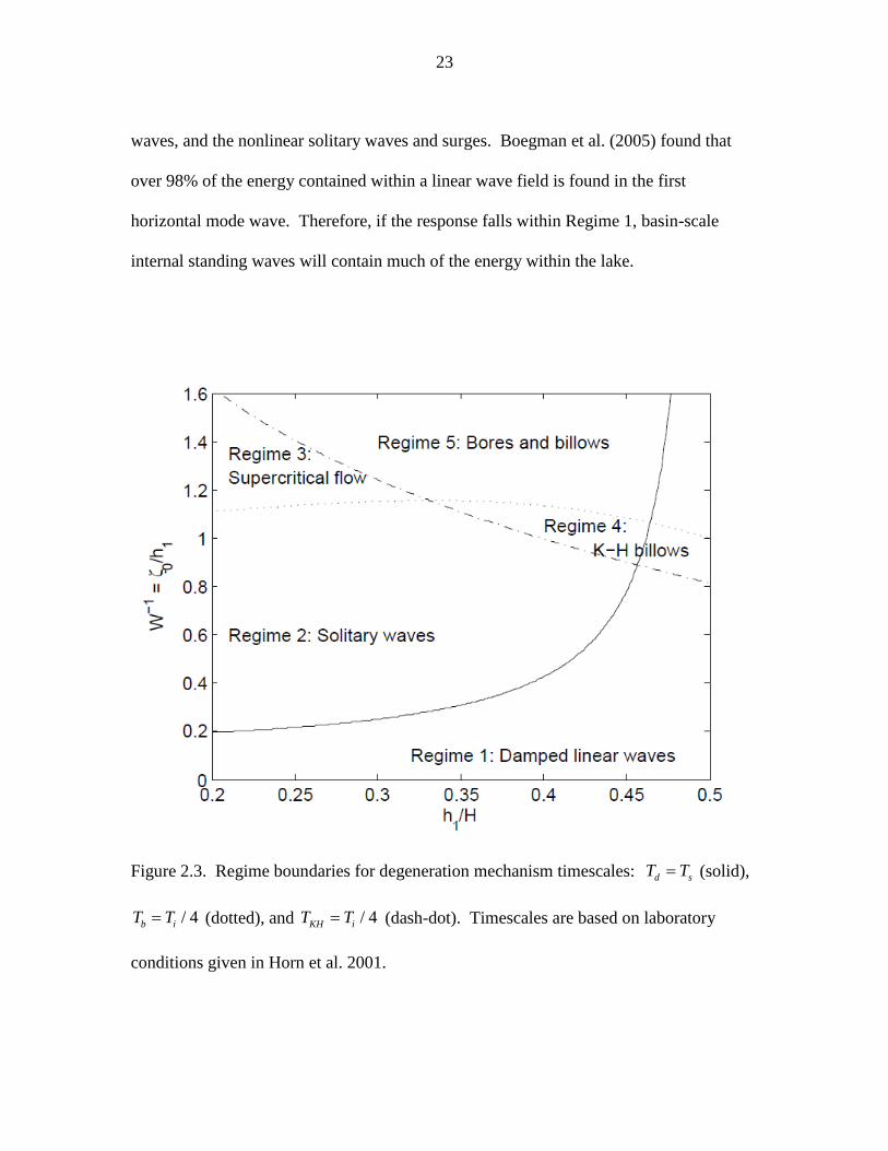
Depending upon the ordering of the timescales, five possible regimes can be
defined in which a particular mechanism is expected to dominate: i) damped linear
waves, ii) solitary waves, iii) supercritical flow, iv) K-H billows, and v) bores and
billows. The boundaries of these regimes are expressed in terms of the Wedderburn
number and the ratio of the internal wave amplitude and the surface layer (Fig 2.3). All
mechanisms excluding the formation of K-H billows depend on lake-specific variables.
As a result, timescales and corresponding figures change depending upon the individual
characteristics of a lake, such as size and stratification.
Comparisons between predictions given by the timescale analysis to laboratory
experiments and field measurements confirmed its applicability (Horn et al., 2001). For
all depth ratios during the experiment, W > 5 indicated energy loss due to damped linear
waves, as the internal wave is damped before it can steepen and evolve into solitons.
Therefore, outside of Regime 1, linear wave theory no longer applies. For weak forcing (
1 0.3W in the experiment) an internal standing seiche was generated and eventually
damped by viscosity. Moderate forcing ( 10.3 1W ) resulted in the production of
internal solitary waves and internal surges.
Boegman et al. (2005) expanded on the laboratory work conducted by Horn et al.
(2001), particularly in quantifying temporal distribution of energy between standing
23
waves, and the nonlinear solitary waves and surges. Boegman et al. (2005) found that
over 98% of the energy contained within a linear wave field is found in the first
horizontal mode wave. Therefore, if the response falls within Regime 1, basin-scale
internal standing waves will contain much of the energy within the lake.
Figure 2.3. Regime boundaries for degeneration mechanism timescales: d sT T (solid),
/ 4b iT T (dotted), and / 4KH iT T (dash-dot). Timescales are based on laboratory
conditions given in Horn et al. 2001.
24
Lake Modeling
To properly represent the energy flux path within a lake, basin-scale motions must
be accurately reproduced. Simple energy arguments (Imberger, 1998) show that an
important component of vertical mass flux in a stratified lake is through the benthic
boundary layer, which is sustained initially by high-frequency internal waves breaking on
the slopes and later by seiche-generated turbulence in the hypolimnion. Therefore, small
errors in modeling the vertical transport will accumulate into large errors in the evolution
of the density struture, resulting in poor representation of the long-term evolution of
physics and ecology of a lake (Hodges et al., 2000). Thus, accurate modeling of mixing
requires correct modeling of the internal wave field. Simple models must accurately
incorporate the effects due to wind forcing, stratification, and basin shape, while complex
models should also include the effects due to surface thermodynamics and variable
bathymetry. This section will present the governing equations involved in lake and
oceanic environments and present the numerical methods involved with three-
dimensional modeling as a viable solution to accurately account for the complexities
involved in predicting lake response.
Governing Equations
The governing equations for lake and coastal ocean systems are the equations for
conservation of momentum and conservation of mass. When neglecting the effects of
rotation, the conservation equations for a Newtonian fluid are given by
25
2Dp g
Dt
uu (2.26)
and
1 D
Dt
u 0 (2.27)
with pressure p , density , and viscosity ; the time substantial derivative /D Dt gives
the rate of change following the fluitd motion, such that
D
Dt t
u (2.28)
where the fluid velocity vector can be expressed in terms of the x y z directions as
, ,u v wu . Simplifying the above conservation equations by assuming a Boussinesq
fluid, momentum conservation(2.26) and mass conservation (2.27) can be rewritten by
expanding the substantial derivative (2.28) and Laplace operator, such that
2 2 2
2 2 2
0
1u u u u p u u uu v w
t x y z x x y z
(2.29)
2 2 2
2 2 2
0
1v v v v p v v vu v w
t x y z y x y z
(2.30)
26
0p
g zz
(2.31)
0u v w
x y z
(2.32)
where / is the kinematic viscosity, and x and y momentum are given by the
Navier-Stokes equations in (2.29) and (2.30), respectively. Gravitational forces do not
enter into the momentum equations if acting in a direction perpendicular to the respective
coordinate axis, thus both x and y -directions are taken to be in the horizontal plane with
z in the vertical. The hydrostatic assumption is expressed in (2.31), where advective,
unsteady, and viscous forces have been neglected in favor of a gravity-pressure balance;
the scaling involved is shown in Cushman-Roisin (1994). The result is that pressure
depends on water density, gravity, and the depth of the fluid. The pressure can be
computed from (2.31) as
00
z
p z p g z dz (2.33)
where depth z is the vertical distance in the fluid measured as positive down from the
water surface, and is atmospheric pressure. As 0z , the pressure approaches
atmospheric.
Conservation of mass (2.32), also referred to as the continuity equation, or simply
continuity, assumes the substantial derivative is negligible when compared to the velocity
gradient. The assumption is that the fluid is approximately incompressible, or that a fluid

27
parcel‘s density is constant. As part of the shallow water assumption, x -viscous forces
are negligible compared to z -viscous forces, justified by scaling using continuity.
Limiting the case to a two-dimensional solution, scaling of x -momentum (2.29) results
in both advective terms of the same order of magnitude, but less than the vertical viscous
term, giving
2
2
1u p u
t x z
(2.34)
Equation (2.34) provides a simplified relationship for momentum conservation which can
be used in modeling the lake response and corresponding hydrodynamic flows. Limiting
the solution to a two-dimensional flow field may at first seem to be a step back in terms
of accurately reproducing internal dynamics; however, the assumption will be shown in
the literature to produce accurate results under certain conditions (i.e. a long, narrow
lake).
Analytical Models
Analytical models are useful when considering lake response to wind forcing as
they provide a succinct solution. However, analytical solutions come at a price; many
simplifications and assumptions arise throughout the process. While these assumptions
provide a set of equations which can solve the system explicitly, the inherent
complexities of the system are lost. This section will present the shallow-water

28
equations, which assume the fluid can be represented by layers of constant density in a
system where the depth is much less than the horizontal extent of the fluid (i.e. small
aspect ratio). The first step is to define the simple one-layer case, which can be expanded
to provide the solutions for systems with more layers.
One-Layer
The simplified -momentum equation (2.34) can be used for a basic analytical
solution. First, consider the steady one-layer case, initially neglecting /u t . To
simplify the geometry involved, the lake can be represented by a rectangular basin of
length L , total undisturbed depth H , wind-applied surface stress 0 , surface
displacement s , and effective depth h such that sh H . A further simplification for
evaluating a layered system is to integrate the conservation equations over the depth.
Integration of the viscous term for x-momentum yields
2
02
00
1 1hh
b
u udz
z z
(2.35)
where z here is defined as positive upwards from the lake bottom and b is the shear
along the bottom of the lake and can be assumed negligible (Lighthill, 1969). Integrating
the pressure term in (2.34) using (2.33) for a constant layer density gives
0
1 1h
p hgh h z gh
x x x
(2.36)
29
and combining (2.35)and (2.36) gives
2
0 *uh
x gh gh
(2.37)
Therefore, under steady conditions, the water surface tilt can be expressed in terms of
shear velocity, gravity, and the water depth.
When accounting for unsteady conditions, it is first useful to integrate the
continuity equation over the depth. Integrating the first term and using the Leibniz rule
gives
0 0
( )
h hu h
dz udz u hx x x
(2.38)
where u h is the horizontal velocity evaluated at the water surface. The first term on
the right side of the equation relates the depth-averaged velocity hU by the following
0
h
hUudz H
x x
(2.39)
Integrating the vertical acceleration over the depth yields the vertical velocity evaluated
at the boundaries, and combining (2.38), (2.39), and the vertical velocity at h gives
30
0hU hH w h u h
x x
(2.40)
which is the integrated expression for continuity. To further simplify(2.40) it is useful to
define the water surface as a function ( , , )wS x z t , and then express the surface as the
difference between the elevation and surface displacement ( , ) 0w sS z x t ,
calculated at the free surface sz . Under the assumption that the normal velocity of
fluid at a surface is equal to the normal velocity of the surface, the substantial derivative
is zero when 0wS . Taking the substantial derivative
0w w w w s ss
DS S S Su w u w
Dt t x z t x
(2.41)
As the water surface is defined such that the undisturbed surface is measured at 0z ,
su u h and sw w h under previous notation, and the slope of the surface
displacement is equivalent to the slope of the effective depth. Rearranging the final
solution of (2.41) and combining with (2.40) gives a new definition for continuity
0s hUH
t x
(2.42)
To solve the unsteady case for a one-layer system, express the integral of the time
derivative in (2.34) by using the Leibniz rule but define the upper bound as the sum of the
undisturbed depth and the displacement sh H . Because the magnitude of the

31
surface displacement‘s time derivative is small compared to the time derivative of the
depth-averaged velocity, it can be neglected, resulting in
0
sH
hu Udz H
t t
(2.43)
combining(2.43) with (2.35) and (2.36) gives x -momentum for the unsteady one-layer
case:
2
*h sU ug
t x h
(2.44)
According to (2.44), the depth-averaged velocity depends on the slope of the free water
surface and the wind-applied surface shear. Coupling (2.42) and (2.44) yields a solution
for the velocity hU and free surface displacement s based on the shear velocity *u .
Two-Layer
Utilizing the one-layer solution, expanding to a two-layer solution involves much
of the same procedure; however, more variables are introduced to account for additional
layer depths, displacements, and velocities. Suppose subscripts 1 and 2 refer to the top
and bottom layer, respectively. Therefore, let 1h and 2h be the undisturbed thicknesses of
the epilimnion and hypolimnion, 1 and 2 the displacements from the undisturbed
position, and 1 1h and 2 2h the effective thicknesses (Fig 2.4).
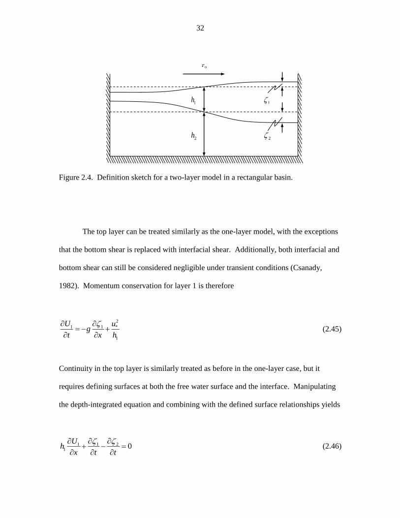
32
Figure 2.4. Definition sketch for a two-layer model in a rectangular basin.
The top layer can be treated similarly as the one-layer model, with the exceptions
that the bottom shear is replaced with interfacial shear. Additionally, both interfacial and
bottom shear can still be considered negligible under transient conditions (Csanady,
1982). Momentum conservation for layer 1 is therefore
2
1 1 *
1
U ug
t x h
(2.45)
Continuity in the top layer is similarly treated as before in the one-layer case, but it
requires defining surfaces at both the free water surface and the interface. Manipulating
the depth-integrated equation and combining with the defined surface relationships yields
1 1 21 0
Uh
x t t
(2.46)
1h
2h
1
1
2
0
0
33
When writing conservation of momentum for layer 2, the boundary pressure
cannot be assumed to be atmospheric. Rather, as 2z h , the pressure at the interface
should be given by (2.33). It is useful to express the integral bounds as the sum of the
undisturbed depth and the displacement, for when differentiating with respect to x , only
the displacement terms remain, giving
2 2 1
0
1 pg g
x x x
(2.47)
By integrating x -momentum over the depth, both viscous terms can be neglected as their
respective magnitudes are small compared to the pressure terms. The kinematic shear
stress, which is analogous to the viscous terms, is assumed to vary linearly throughout the
mixed layer from a value of 2
*u at the free surface to zero at the base of the mixed layer
(Monismith, 1985). Therefore, viscous terms are neglected when considering anything
but the surface layer.
Using (2.47) in the momentum expression for the bottom layer gives
2 1 2Ug g
t x x
(2.48)
and continuity for the bottom layer is given by
2 22 0
Uh
x t
(2.49)

34
The two layer system can now be modeled analytically by using (2.46) - (2.49), given an
initial density profile and information related to the environmental forcing (i.e. wind-
applied shear).
Simplifying the above momentum and continuity equations by assuming steady
conditions yields an important relationship. Under steady conditions, the only terms
remaining in (2.48) are the pressure terms given in (2.47). Rearranging the expressions
to compare free water and interface displacements yields
02
1
/
/
x
x
(2.50)
The tilting of the free surface is often referred to as the barotropic response, while
baroclinic response refers to internal responses caused by layer interfaces. The required
time for equilibrium conditions for interface set-up is / 4iT , as the effects of the end
walls have not made themselves felt for / 4it T (Spigel and Imberger, 1980). Here, iT
is the wave period of the thi vertical mode, which increases with increasing modes
(Monismith, 1985). Stevens and Imberger (1996) gave the non-dimensional ratio
delineating whether the wind duration sufficient to allow adequate tilting to develop the
thi mode as 4 /w iT T , where wT is the wind duration. Therefore, a time-series of *u should
first be low-pass filtered with a cutoff frequency of 4 / iT before W or NL is calculated
(Stevens et al., 1997).
Three important observations can be made with the results from (2.50). First, the
interfacial tilt is always opposite (or negative) of the free surface tilt. Therefore, as the
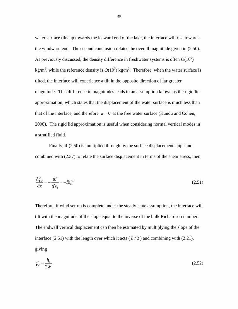
35
water surface tilts up towards the leeward end of the lake, the interface will rise towards
the windward end. The second conclusion relates the overall magnitude given in (2.50).
As previously discussed, the density difference in freshwater systems is often O(100)
kg/m3, while the reference density is O(10
3) kg/m
3. Therefore, when the water surface is
tilted, the interface will experience a tilt in the opposite direction of far greater
magnitude. This difference in magnitudes leads to an assumption known as the rigid lid
approximation, which states that the displacement of the water surface is much less than
that of the interface, and therefore 0w at the free water surface (Kundu and Cohen,
2008). The rigid lid approximation is useful when considering normal vertical modes in
a stratified fluid.
Finally, if (2.50) is multiplied through by the surface displacement slope and
combined with (2.37) to relate the surface displacement in terms of the shear stress, then
212 *
1
b
uRi
x g h
(2.51)
Therefore, if wind set-up is complete under the steady-state assumption, the interface will
tilt with the magnitude of the slope equal to the inverse of the bulk Richardson number.
The endwall vertical displacement can then be estimated by multiplying the slope of the
interface (2.51) with the length over which it acts ( / 2L ) and combining with (2.21),
giving
1
2e
h
W (2.52)

36
where e is the vertical displacement (e.g. of a fluid parcel or isotherm) at the lake‘s
windward end and W is the Wedderburn number. Equation (2.52) shows that upwelling
( 1e h ) occurs when 1 2W .
Stevens and Lawrence (1997) compared estimated displacements based on the
Wedderburn number to measured lake response from four lakes of different size: a short
deep lake (Sooke Lake Reservoir), a long deep lake (Kootenay Lake), a very short, very
deep lake (Brenda Pit Lake) and a short shallow lake (Chain Lake). The model provided
postive results for Sooke Reservoir but tended to underpredict response for Brenda Pit
and Chain Lake. The longer wave period of Kootenay Lake limited the applicability of
the model, as the seiche experienced greater variations in forcing. Therefore, the
Wedderburn number can be used to predict endwall displacements within an order of
magnitude. Outliers in the observed data were related to weak deflections or continuing
wave activity from previous events. The authors also compared the values of W and NL
to try to distinguish different vertical mode response; however, there were no periods
where NL was differing by an order of magnitude from W ( NL reached a maximum of
4W for Kootenay Lake). Therefore, results were deemed to be primarily mode one.
Heaps and Ramsbottom (1966) gave solutions for the two-layer case similar to
(2.45), (2.46), (2.48), and (2.49) but accounted for damping by including a separate
bottom shear force. The bottom friction was defined as proportional to the horizontal
flow in the bottom layer. The solution for the two-layer case with bottom friction was
applied to field observations from Lake Windermere with good results for the
displacement of the layer interface (see Fig. 11 in Heaps and Ramsbottom, 1966). The
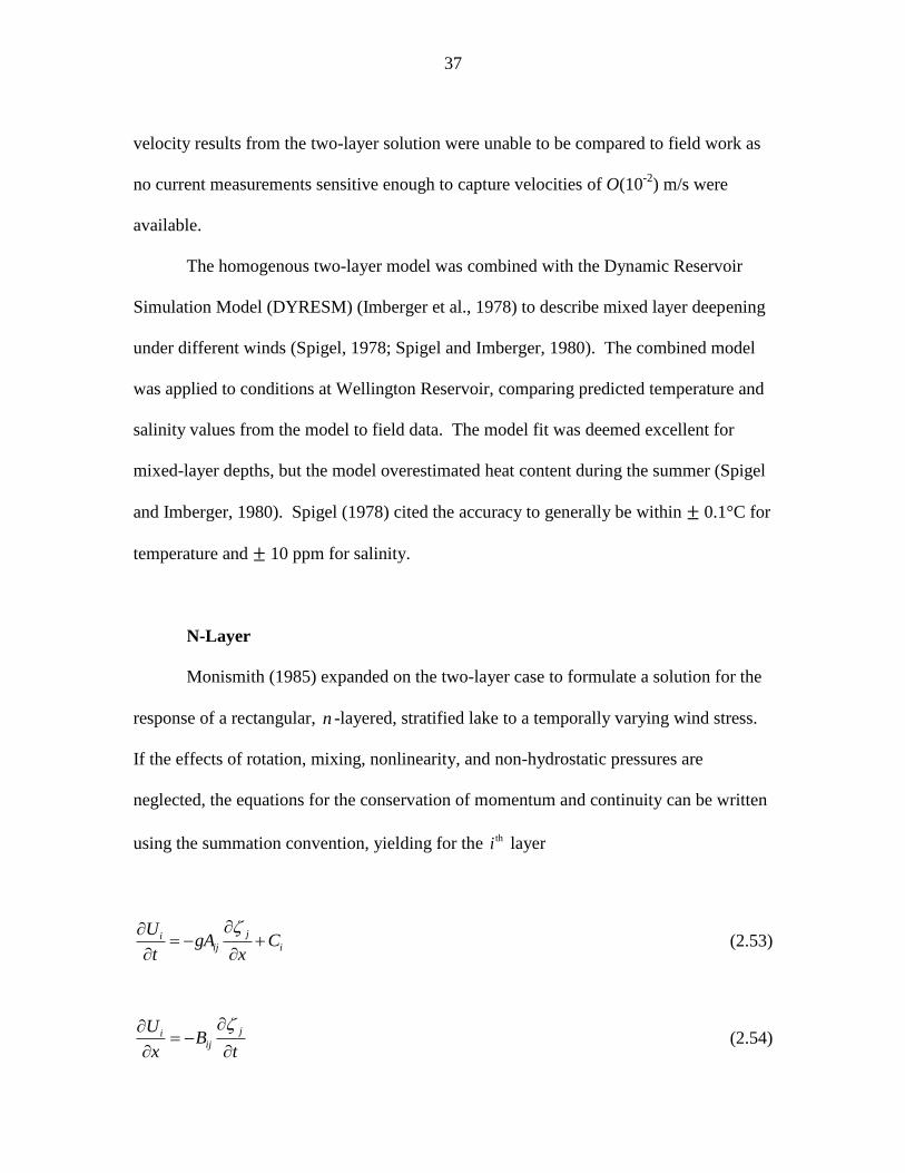
37
velocity results from the two-layer solution were unable to be compared to field work as
no current measurements sensitive enough to capture velocities of O(10-2
) m/s were
available.
The homogenous two-layer model was combined with the Dynamic Reservoir
Simulation Model (DYRESM) (Imberger et al., 1978) to describe mixed layer deepening
under different winds (Spigel, 1978; Spigel and Imberger, 1980). The combined model
was applied to conditions at Wellington Reservoir, comparing predicted temperature and
salinity values from the model to field data. The model fit was deemed excellent for
mixed-layer depths, but the model overestimated heat content during the summer (Spigel
and Imberger, 1980). Spigel (1978) cited the accuracy to generally be within 0.1°C for
temperature and 10 ppm for salinity.
N-Layer
Monismith (1985) expanded on the two-layer case to formulate a solution for the
response of a rectangular, n -layered, stratified lake to a temporally varying wind stress.
If the effects of rotation, mixing, nonlinearity, and non-hydrostatic pressures are
neglected, the equations for the conservation of momentum and continuity can be written
using the summation convention, yielding for the thi layer
jiij i
UgA C
t x
(2.53)
jiij
UB
x t
(2.54)
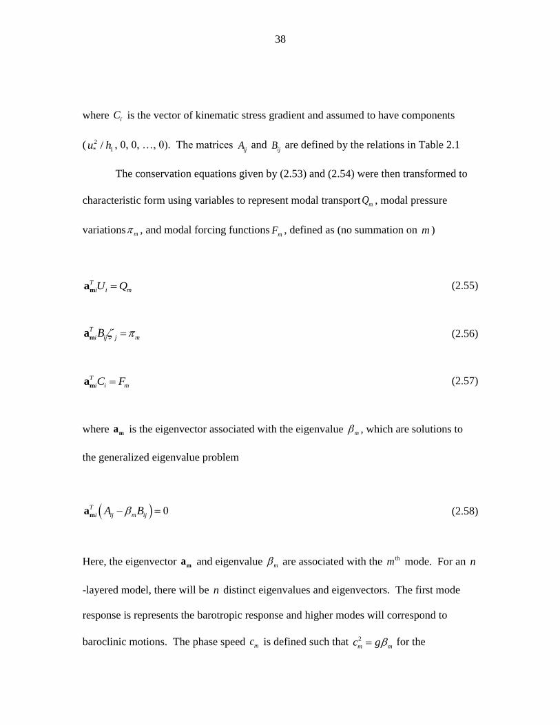
38
where iC is the vector of kinematic stress gradient and assumed to have components
( 2
* 1/u h , 0, 0, …, 0). The matrices ijA and
ijB are defined by the relations in Table 2.1
The conservation equations given by (2.53) and (2.54) were then transformed to
characteristic form using variables to represent modal transport mQ , modal pressure
variations m , and modal forcing functionsmF , defined as (no summation on m )
T
i i mU Qma (2.55)
T
i ij j mB ma (2.56)
T
i i mC Fm
a (2.57)
where ma is the eigenvector associated with the eigenvalue m , which are solutions to
the generalized eigenvalue problem
0T
i ij m ijA B m
a (2.58)
Here, the eigenvector ma and eigenvalue m are associated with the thm mode. For an n
-layered model, there will be n distinct eigenvalues and eigenvectors. The first mode
response is represents the barotropic response and higher modes will correspond to
baroclinic motions. The phase speed mc is defined such that 2
m mc g for the
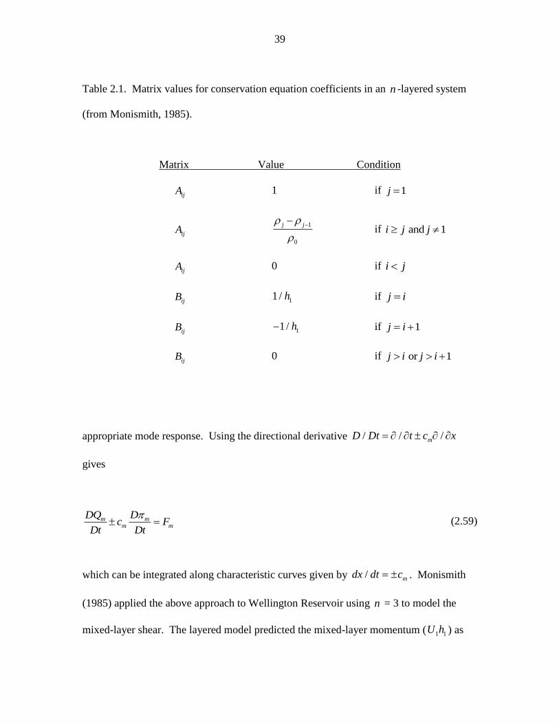
39
Table 2.1. Matrix values for conservation equation coefficients in an n -layered system
(from Monismith, 1985).
Matrix Value Condition
ijA 1 if 1j
ijA 1
0
j j
if and 1i j j
ijA 0 if i j
ijB 11 / h if j i
ijB 11/ h if 1j i
ijB 0 if or 1j i j i
appropriate mode response. Using the directional derivative / / /mD Dt t c x
gives
m mm m
DQ Dc F
Dt Dt
(2.59)
which can be integrated along characteristic curves given by / mdx dt c . Monismith
(1985) applied the above approach to Wellington Reservoir using n = 3 to model the
mixed-layer shear. The layered model predicted the mixed-layer momentum ( 1 1U h ) as

40
0.55 m2/s, which is comparable to the observed value of approximately 0.5 m
2/s given by
Imberger (1985). However, the model could not accurately predict maximum velocities,
two cases of different vertical structure yielded maximum shear of 0.44 and 0.065 m/s,
while Imberger (1985) gave mixed-layer velocities of about 0.1 m/s. Thus, while the
model failed to predict mixed-layer shear, it could properly estimate the gain in mixed-
layer momentum, which Monismith (1985) attributed to the successful prediction of fluid
response timing.
The layered model can estimate end-wall displacements (Stevens and Lawerence,
1997) and, by incorporating damping due to bottom friction, accurately estimate dynamic
isotherm displacements over a five-day simulation (Heaps and Ramsbottom, 1966). It
has been combined with a vertical mixing model to accurately estimate temperature and
salinity profiles over a year (Spigel, 1978; Spigel and Imberger, 1980), and it can
estimate fluid response and mixed-layer momentum (Monismith, 1985). The solution of
an n -layered rectangular stratified lake has been provided (Monismith, 1985) such that
higher modal responses can be solved for systems with more vertical layers.
Numerical Models
The previous section dealt with analytical models as a tool for evaluating lake
response. Analytical solutions are indeed useful; however, several simplifying
assumptions are necessary in order to solve the system. The assumptions vary from
representing the lake with a rectangular basin, to limiting the solution to a two-
41
dimensional solution and neglecting convective and viscous terms in the momentum
equations. To preserve the complexities within the system, numerical models have been
developed which retain more details than analytical models. This section will outline
selected numerical schemes used in hydrostatic models, highlight several applications of
a particular hydrostatic model, discuss effects related to grid resolution in numerical
modeling, and introduce the development and application of non-hydrostatic models.
Hydrostatic Models
Casulli and Cheng (1992) developed a general three-dimensional model TRIM-
3D (Tidal, Residual, and Inter-tidal Mudflat), which solves the Navier-Stokes equations
with the hydrostatic assumption and a semi-implicit finite difference method. The TRIM
method can be classified as a two-level, single-step method which uses two time levels of
information and takes a single model step to integrate forward in time. The gradient of
the water surface elevation in the momentum equations, the velocity in the free surface
equation, and the vertical mixing terms are discretized implicitly. However, the
convective, Coriolis, and horizontal viscosity terms in the momentum equations are
discretized explicitly. The free surface is solved by using the conjugate gradient method
at every time step. Once the free surface is known throughout the domain, cells near the
free surface are defined as either flooding or drying, which allows the model to
accurately account for permanently dry areas (e.g., islands and mud flats), as well as
boundary shorelines which may experience significant changes in water level.
42
Designating a cell as either wet or dry simplifies the computer algorithm by increasing
the computational efficiency (Casulli and Cheng, 1992).
Saggio and Imberger (1998) used the TRIM-3D method to help differentiate
various wave modes recorded at lower frequencies from field data. Power spectra were
constructed from both field and numerical model results and compared across various
frequencies. The main frequency peaks associated with basin-scale motions were well
produced, but higher frequencies in the numerical spectrum deviated from the measured
values. The authors reported the discrepancy for higher frequency motions was attributed
to coarse (500 m) horizontal grid size and lack in the model of the generation
mechanisms provided by the variability in the real winds.
Hodges et al. (2000) adapted the fundamental numerical scheme from TRIM-3D
with modifications for accuracy, scalar conservation, numerical diffusion, and
implementation of a mixed-layer turbulence closure. The Estuary, Lake, and Coastal
Ocean Model (ELCOM) has demonstrated reasonable short-term models (approximately
4 wave periods) of hydrostatic internal waves (Hodges et al., 2000) and longer-term
simulations of circulations with density structure (Laval et al., 2003b). ELCOM provides
a semi-implicit solution of the hydrostatic, Boussinesq, Reynolds-averaged Navier-Stokes
equations and scalar transport equations (Hodges et al., 2006). The grid is a Cartesian z-
coordinate mesh using an Arakawa-C grid stencil: velocities are defined on cell faces
with free-surface height and scalar concentrations on cell centers. The model also
includes a filter to control the numerical diffusion of potential energy (Laval et al.,
2003a).
43
ELCOM computes a model time step in a staged approach consisting of (1)
introduction of surface heating/cooling in the surface layer, (2) mixing of scalar
concentrations and momentum using a mixed-layer model, (3) introduction of wind
energy as a momentum source in the wind-mixed layer, (4) solution of the free-surface
evolution and velocity field, (5) horizontal diffusion of momentum, (6) advection of
scalars, and (7) horizontal diffusion of scalars. For details on the numerical method, see
Hodges et al. (2000).
To evaluate model performance, ELCOM output was compared to field
observations from Lake Kinneret (Hodges et al., 2000), focusing on the reproduction of
basin-scale waves, wave amplitudes, and the depth of the base of the mixed layer. The
existence and reproduction of internal waves in model space can be supported by
comparing isotherm displacement spectra between measured and model isotherm
movement. ELCOM resolved the basin-scale waves, but showed a rapid divergence of
the model and field signals for higher frequencies, which is a consequence of the
dissipation occurring at numerical grid and temporal scales in the model.
A heat budget was analyzed to determine if ELCOM could accurately replicate
the surface heat fluxes. Over the course of a 12 d simulation, the cumulative change is
less than 0.004% of the total heat budget. The error per time step amounted to less than
10-5
°C in each grid cell, which is on the level of the truncation error (Hodges et al.,
2000). The field data were compared to the model output in terms of wave amplitudes,
depth of the mixed-layer, and phase angle. ELCOM captured the nature of the peaks and
troughs in the thermocline signature and the depth of the wind-mixed layer; however, the
wave phases, amplitudes, and steepness differed. ELCOM led the field data by as much
44
as 5 h (25% of the base period ) and lagged up to 2.5 h (10% of base period). Overall,
ELCOM was shown to successfully recreate basin-scale motions in the lake, but it could
not resolve higher frequency waves due to restrictions in the spatial and temporal grid
resolution.
Applications of Numerical Models
The importance of ELCOM as a numerical model can best be described with its
wide range of applications. More specifically, the successful matching of model output
to measured field data allows ELCOM to extrapolate upon known scenarios in order to
incorporate hypothetical situations. Several applications of ELCOM are presented to
provide a better understanding and appreciation of the importance of lake modeling.
ELCOM has been used to model the dynamics in a salt-stratified lake (Lake
Maracaibo) because of concerns with highly saline water and anoxic conditions in the
hypolimnion (Laval et al., 2005). Field data from Lake Maracaibo show a persistent
basin-scale cyclonic gyre which dominated the lake‘s circulation and resulted in doming
of isopycnals (Parra-Pardi, 1979). ELCOM was therefore compared to field data in terms
of reproducing circulation currents and saline levels, particularly the doming of
isopycnals. Simulations reproduced the observed cyclonic gyre from field studies, and
while the isohaline doming was slightly underestimated, the model was able to reproduce
the basic characteristics in the salinity profiles (Laval et al., 2005).
Often, meteorological field data comes from one source and ELCOM must
therefore use a horizontally uniform wind field (e.g., Hodges et al., 2000; Vidal et al.,

45
2005; Chung et al., 2009), while using multiple wind gauges allows for spatially-varying
wind fields (e.g., Leon et al., 2005; Rao et al., 2009). To evaluate the effects of spatial
variations in the wind field on numerical model results, simulations were conducted using
uniform and non-uniform wind fields (e.g., Laval et al., 2003; Laval et al., 2005) and
compared in terms of the model‘s ability to reproduce circulation or the internal wave
field. A non-uniform wind field more accurately reproduced the mean circulation in the
surface layer for both drifter studies (Laval et al., 2003b) and in the case of setting up
gyres which lead to the doming of isopycnals (Laval et al., 2005). However, applying a
uniform wind field derived from the horizontally averaged wind stress improved the
model‘s prediction for isotherm displacements and phase coherency (Laval et al., 2003).
Vidal and Casamitjana (2008) studied the response of a lake to a wind field in an
attempt to capture higher vertical mode waves. The authors compared field data to model
output from ELCOM and found excellent agreement for the velocity field, vertical
isotherm displacement, and evaluated the internal wave field using a power spectral
density plot. ELCOM reproduced the modal response of the V2 wave quite well;
however, the displacements associated with the V3 modal response were damped because
of the model‘s artificial dissipation. Additionally, ELCOM was used to find the natural
periods of the modes by removing wind forcing and designating initial tilting of the
isotherms. The results from the model indicate far different periods for the V2 and V3
modes than was previously predicted by solving the eigenvalue problem (i.e., Vidal et al.,
2005).
Chung et al. (2009) used ELCOM to simulate turbid density inflows into a
stratified reservoir with the goal of integrating real-time turbidity monitoring and

46
modeling systems to develop effective decision-making processes for controlling turbid
inflows. For the numerical simulations, ELCOM was paired with the Computational
Aquatic Ecosystem Dynamics Model (CAEDYM), which was used to simulate particle
dynamics by accounting for settling and resuspension rates of non-cohesive suspended
sediments. Temperature and turbidity profiles were compared between field observations
and numerical simulations by calculating the mean absolute error (MAE) and the root
mean square error (RMSE). The average results for temperature were 1.5°C for MAE
and 1.8°C for RMSE, and the average results for turbidity were 35 NTU for MAE and
41.9 NTU for RMSE. Overall, ELCOM-CAEDYM provided excellent agreement with
field measurements of turbidity propagation in the reservoir, although the model tended
to under-predict the suspended sediment concentrations.
The coupling of physical and biological processes through the use of ELCOM-
CAEDYM also has implications in modeling nutrient cycling and distribution (e.g.
Spillman et al., 2007). The model was used to assess the role of nutrient inputs, basin-
wide nutrient fluxes, and the response of phytoplankton concentrations and distribution
within the Northern Adriatic Sea. To evaluate model success, simulated salinity and
temperature profiles were compared to measured values, giving r2 values of 0.908 and
0.863 for salinity and temperature, respectively. The model accurately reproduced the
temperature field and the free water surface but overestimated the distribution
chlorophyll concentrations within the basin and slightly underestimated the observed
peak concentrations. Despite the discrepancies, the authors were able to use the model
results to indicate possible nutrient reduction methods for water bodies emptying in the
Northern Adriatic Sea.

47
The coupling of ELCOM-CAEDYM can be used as a hydrodynamic/chemical
model to reproduce the thermal structure and pattern circulation in lakes (e.g. Leon et al.,
2005; Rao et al., 2009), with the goal of using modeled hydrodynamic fluxes to estimate
nutrient transport and distribution. Rao et al. (2009) cited considerable model skill when
comparing model output to measured field data, with respect to circulation, free surface
level, and thermal structure in the lake. ELCOM was able to match measured water level
variabilities within 90%. The model was able to provide circulation patterns within the
lake, in particular, recreating two rotating gyres in the lake interior (Leon et al., 2005).
Both papers suggested the model can accurately describe flow and transport of material
required for detailed water quality simulations.
Effects of Grid Resolution in Numerical Models
While numerical models have been shown to accurately resolve internal dynamics
in lakes and other similar environments, numerical error created throughout the
simulation can compromise the model‘s results. The most significant forms of error to
consider when dealing with numerical models are typically seen in the form of numerical
diffusion and numerical dissipation. Numerical diffusion is caused by a density-transport
truncation error while a truncation error in the momentum equation results in numerical
dissipation (Hodges et al., 2006).
Numerical diffusion can cause cumulative effects in a 3D model, slowly reducing
the background stratification (i.e., altering the background potential energy) and
thickening the metalimnion. Unstable numerical discretization methods rely on

48
additional viscous or diffusive terms through truncation errors (Rueda et al., 2007).
ELCOM was implemented with a turbulence closure method to reduce artificial
diffusion; however, cumulative numerical diffusion limits the use of the model for long-
term simulations (Hodges et al., 2000).
Background potential energy is classified as the minimum potential energy
attainable through adiabatic redistribution of the density field (Lorenz, 1955). Thus, in
order to maintain vertical stratification, methods which reduce change in background
potential energy over the course of a time step could successfully reduce numerical
diffusion. One such method is a pycnocline sharpening filter based on the inverse Z
transform of a linear response to a Heaviside step function (Laval et al., 2003). For a
year-long ELCOM simulation, the pycnocline filter reduced artificial mixing due to
numerical diffusion and retained the metalimnion stratification better than the unfiltered
simulation.
However, assessing the change in background potential energy requires additional
computation time and a closed basin with no mass fluxes into or out of the model domain
(Yeates et al., 2008). Therefore, the pycnocline filter was further refined by comparing
model results to high-resolution thermistor chain data collected in the field. The
simulation results using the new thermistor chain data assimilation technique leads to
more accurate long-term model performance and addresses mixing processes not resolved
by the current mixing model in ELCOM.
While numerical diffusion can hinder model performance by reducing the
background stratification, the damping of internal motions due to numerical dissipation
can under-predict the lake response. While ELCOM has been shown to qualitatively

49
reproduce the internal wave structure in terms of peaks and troughs in the motions, the
model output exhibited decreased amplitudes and damping of internal waves (Hodges et
al., 2000; Vidal and Casamitjana, 2008; Gomez-Giraldo et al., 2006). There are further
complications relating to interrelationships between numerical diffusion and numerical
dissipation; a theoretically perfect solution to the momentum equation may lose kinetic
energy due to numerical diffusion of mass (Hodges et al., 2006).
Other consequences involved with modeling arise from representing naturally
smooth features with grids of finite length scales. Due to the nature of the z-coordinate
system in numerical modeling, bottom boundaries may experience significant changes in
elevation for steep lake bottoms. The main concern associated with z-coordinate models
is that the stair-step representation can introduce abrupt local topography, which is
known to generate strong form drag (Edwards et al., 2004). Form drag contributes to
higher and more widespread mixing than frictional drag (Moum and Nash, 2000). To
evaluate the effect of form drag, ELCOM was compared to an analytical solution by
modeling a two-dimensional wave train over a non-uniform bottom boundary
(Simanjuntak et al., 2009). The authors found that weak slopes and low wavenumber
internal waves can be well resolved; however, higher mode waves exhibit problems with
refraction along the grid edge.
Hodges et al. (2006) estimated values of numerical diffusion and dissipation for
nonlinear internal waves using ELCOM to simulate a simple unforced standing wave in a
diffusionless, inviscid fluid. By assuming no molecular diffusion or dissipation, changes
in the background potential energy BE and the dynamic energy DE could be attributed
solely to numerical diffusion and numerical dissipation, respectively. Simulations were

50
modeled past the time scale to the onset of steepening s , which is similar to the
steepening timescale sT given by Horn et al. (2001). Results show numerical dissipation
(i.e., loss of DE ) becomes prevalent after time s .
To compare results, Hodges et al. (2006) grouped simulations into ―dissipation-
dominated‖ and ―diffusion-dominated‖ based upon their changes in DE and BE ,
respectively, and found for times 0 st
2 21/3 0
2
0
g
zRi
T
(2.60)
2 21/3 0
2
0 0
g
z xRi
T
(2.61)
21/3 0 0
2
0 0
g
z xRi
T
(2.62)
2 21/3 0
2
0 0
g
z xRi
T
(2.63)
where gRi is the gradient Richardson number, 0 is the interface (or metalimnion)
thickness, 0 is the initial wavelength, T is the period of the V1H1 wave, x is the
horizontal grid size, z is the vertical grid size, is numerical diffusivity, and is
numerical viscosity, and subscripts and correspond to diffusion and dissipation-
51
dominated systems, respectively. By comparing to , a scaling parameter was
defined as
1 2
1 2
1h h
Hh h
(2.64)
such that C corresponded to a dissipation-dominated system and C to a
diffusion-dominated system. Then for a dissipation-dominated system with a thin upper
layer 10 / 2h H
2
1 2 2 1
2 2
h
H
(2.65)
where the term arises from (2.61) and (2.63), such that
12 2
2 2
0 0 0 0
1C
z x z x
(2.66)
where 8.5C was found to correctly place 93% of dissipation-dominated results in the
regime C and 94% of diffusion-dominated results in the regime C . Therefore,
(2.64) - (2.66) can be used to determine whether a set of model conditions is likely to be
dominated by numerical diffusion or dissipation using ELCOM.
52
Non-Hydrostatic Models
Three-dimensional hydrostatic models are commonly used to predict the basin-
scale internal wave field (e.g., Hodges et al., 2000; Laval et al., 2003; Laval et al., 2005;
Chung et al., 2009). However, internal wave dynamics can often be nonlinear, especially
at smaller scales, and the hydrostatic assumption may no longer be valid (Hodges et al.,
2006). The complication when considering nonlinear waves lies with the spatial scale of
the internal wave spectrum: 1,000-10,000 m for the basin-scale waves, down to ~100-
1,000 m for solitons, and about 10-100 m for shear instabilities (Botelho and Imberger,
2007). Unless horizontal grid scales are on the order of 1/10th
of the water depth, it is
unlikely that a 3D non-hydrostatic model will resolve the non-hydrostatic motions
(Hodges et al., 2006).
Therefore, models at high enough resolution to simulate nonlinear waves will
provide further insight into the flux path of energy in lakes. While non-hydrostatic
models are important in terms of reproducing internal wave activity at larger than basin-
scale frequencies, the description of non-hydrostatic models at great detail is outside the
scope of this work. However, to illustrate their applicability and the current stage of their
development, examples of non-hydrostatic models are presented.
Examples and Applications of Non-Hydrostatic Models
Botelho et al. (2009) developed a grid switching strategy for ELCOM where the
hydrostatic model predicts basin-scale internal waves but switches to a higher resolution
53
grid when the flow becomes non-hydrostatic in order to resolve the internal wave field
utilizing additional numerical techniques (i.e., Bi-CGSTAB solver). The hybrid
hydrostatic/non-hydrostatic grid-switching model was compared to measured field data
from a small lake (Lake Pusiano) to assess the model‘s accuracy. Hydrostatic
calculations were accomplished on a 100x100 m and 20x20 m horizontal uniform grid.
The non-hydrostatic grid size varied from 20x20 m and 10x10 m uniform grid to a 1x1 m
non-uniform grid. Overall, the non-hydrostatic waves were resolved well with the finer
grid resolution, but the model could not reproduce the measured waves at frequencies
approaching the buoyancy frequency. However, utilizing models at such high resolution
requires a much larger amount of run time: the 1x1 m grid took approximately two days
to run for a one-hour simulation.
Another example of non-hydrostatic model is a three-dimensional numerical
model which solves the Boussinesq, Reynolds-averaged Navier-Stokes equations using a
-coordinate system (Kocyigit and Falconer, 2004). The behavior of the model was
compared to a simple example of a rectangular closed basin example under hydrostatic
conditions and to a full-scale example using measured field data from a small lake
(Esthwaite Water). The model performed well when compared to the rectangular basin in
terms of reproducing velocity, pressure, and circulation within the system. When
compared to the full-scale example, the ability of the model to predict velocities
decreased significantly near the boundaries. Furthermore, Coriolis forces had a
pronounced effect on the circulation patterns, except close to lateral boundaries (Kocyigit
and Falconer, 2004). To increase model accuracy, the authors stated improvements in
representing the lateral boundary interactions were necessary.

54
Summary
Stratification in lakes and reservoirs has been shown to restrict and inhibit vertical
mixing and control the spatial variability of nutrients, dissolved oxygen, and other
dissolved substances. The energy flux path consists of momentum transfer from wind-
applied surface shear to the internal wave field, ultimately degenerating or dissipating.
Internal dynamics within a stratified body therefore has far-reaching implications in
overall water quality and aquatic biological communities.
Analytical solutions have been developed which separate the stratified body into
layers of constant density and represent the lake as a rectangular basin. These solutions
have been shown to accurately recreate the thermal structure and internal motions due to
environmental forcing. Often systems are represented by a two or three-layer system,
either treating the thermocline as an interface, or of finite thickness and uniform density.
Numerical models play an important role in representing hydrodynamics in lakes
and coastal oceans. Currently, hydrostatic models have received much of the attention, as
they have proven that they can reproduce basin scale motions at reasonable model
computational times. Three-dimensional models have been shown to accurately
reproduce thermal structures and circulation patterns. The coupling of ELCOM as a
hydrodynamic model with biological/chemical models such as CAEDYM is providing
new opportunities for the use of numerical models outside the physical oceanography and
limnology communities. Much of success of 3D models has been well documented;
however, the comparisons made between real and simulated events (especially those of

55
the internal wave field and surface layer circulation) is often limited to qualitative
discussion. It is therefore one of the aims of this work to quantify model performance by
comparing model results to field observations.
While 3D models have been shown to be accurate in predicting many facets of
hydrodynamic flows, numerical modeling is limited by the presence of numerical error:
numerical diffusion erodes stratification and numerical viscosity has been shown to
dampen and dissipate internal motions. Much work has been done to circumvent
numerical diffusion with filters, new numerical techniques, and incorporating measured
data into model output, but the issue is far from resolved. Scaling has offered estimates
for numerical diffusion and viscosity, but these experiments were conducted on
simplified basins with simple waves. Therefore, by considering the effects of spatial and
temporal resolution on model predictions, this work will evaluate the role of numerical
error in model results through comparison to field observations.

56
CHAPTER 3: METHODS
Introduction
Chapter 3 describes the experimental methods, simulation techniques, and data
analysis procedures. An objective of the completed work is to classify the response of a
lake to external forcing and evaluate the effects of spatial and temporal resolutions in a
three-dimensional numerical model on reproducing measured events. The response of
the lake will be evaluated by means of the meteorological conditions, internal wave field,
and power spectra. To accomplish this objective, meteorological conditions were
measured using a Lake Diagnostic System (LDS) and used to quantify the applied wind
forcing. Additionally, the thermal structure of the lake was measured using multiple
thermistor chains at various locations throughout the lake. The Wedderburn and Lake
numbers combine the forcing stress and the lake‘s thermal structure into dimensionless
numbers which can be further used to classify a response. Numerical modeling of fully
three-dimensional stratified flows was done using the Estuary, Lake, and Coastal Ocean
Model. A brief overview of the model will be presented, followed with the methods
involved with setting up and running the model. For further details on the numerical
methods and proper procedures for using the model, see Hodges et al. (2000) and Hodges
and Dallimore (2007). Lastly, methods for analyzing field and model results will be
presented.

57
Field Work
The field work was conducted in two lakes over the course of three years. The
summers of 2007 and 2008 were spent at Ada Hayden Lake in Ames, Iowa. West
Okoboji Lake near Arnold‘s Park, Iowa was the site for further field research in 2009. As
part of the fieldwork, several instruments were used to collect data. An overview of each
lake will be presented which will provide information regarding instrument locations and
general characteristics of the water body. A description of the instruments used in the
field is provided, outlining the methods used for deployment and data collection.
Ada Hayden Lake
Ada Hayden Lake (Fig. 3.1) is an abandoned gravel quarry that now provides a
secondary water supply for the City of Ames. It consists of two basins separated by a
shallow shelf (approximately 3 m). All field measurements conducted in the larger,
southern basin. The basin of interest has a surface area of approximately 0.3 km2 and a
maximum depth of about 17 m. The lake is fed through groundwater and surface runoff
which is filtered through a wetland system. During the summer when the stratification of
the lake is fully developed, a 4-5 m well mixed epilimnion overlies a linearly stratified
hypolimnion with a buoyancy frequency N between 25 and 45 cph. Because the shelf
separating the two basins is shallower than the epilimnion, only epilimnetic water is
probably exchanged. Additionally, motorized boats are prohibited on the lake,
minimizing any potential mixing attributed to boat traffic.

58
Figure 3.1. Bathymetric map of Ada Hayden Lake with 4 m contour intervals. Symbols
depicting instrument deployment locations are shown for 2007 (blue) and 2008 (black).
Only two thermistor chains were deployed in 2007.
The lake has steep northern, eastern, and southern sides. The LDS was deployed
near the deepest section of the lake to provide measurements to the lake bottom (Fig.
3.1). Free-standing thermistor chains were deployed near the northeast and southeast
section of the lake. The location for the thermistor chain at the NE corner (T-Chain 52 in
2007, T-Chain 53 in 2008) was selected to be along the primary wind axis. The location

59
for the SE thermistor chain (T-Chain 52 in 2008) was selected because it was at a
comparable depth to T-Chain 1.
West Okoboji Lake
West Okoboji Lake (Fig. 3.2) is a natural lake located in Dickinson County in
northwest Iowa. It acts as a drinking water source for several communities near the lake,
as well as a popular recreation destination for sailing and power boating. It is fed
primarily by groundwater and subterranean springs. West Okoboji Lake has a surface
area of 15.6 km2 and a maximum depth of 41 m. The lake flows into East Okoboji Lake
through Smith‘s Bay through a 3 m deep channel. Because of the stratification of West
Okoboji Lake during the summer months, the structure of the lake consists of a well-
mixed epilimnion, a steep temperature gradient contained within a thick metalimnion,
and weakly stratified hypolimnion. The epilimnion extends well below 3 m, preventing
internal wave action within West Okoboji Lake from interacting with East Okoboji Lake.
As such, West Okoboji Lake is considered to be an enclosed basin in this study.
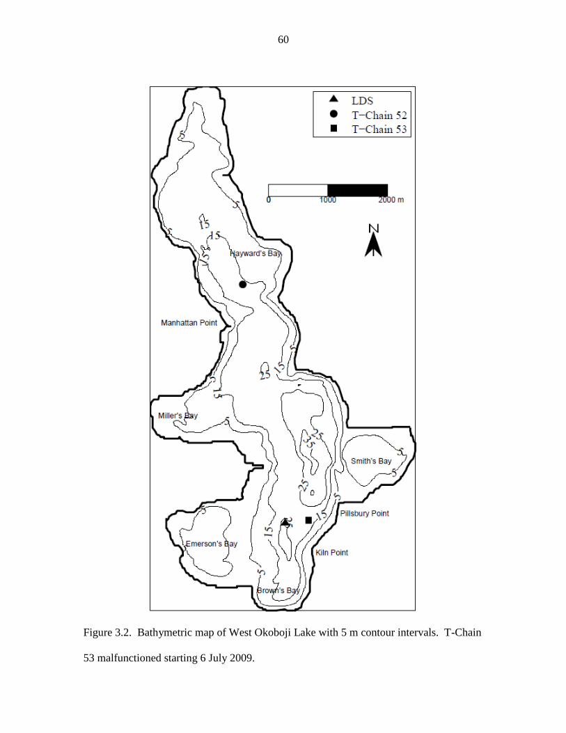
60
Figure 3.2. Bathymetric map of West Okoboji Lake with 5 m contour intervals. T-Chain
53 malfunctioned starting 6 July 2009.

61
The LDS was deployed along the thalweg of the lake in one of the deepest points
of the lake (approximately 27 m), while yet far enough from high boat traffic areas to
maintain safety for both boaters and field instruments. The thalweg—or ―valley way‖—
is the deepest continuous line along the lake bottom. Regulatory hazard buoys with a
mounted one-mile solar amber light (flashing at 1 Hz) were placed around the LDS to
warn boaters of its location. The northern of the two free-standing thermistor chains (T-
Chain 52) was deployed between Manhattan Point and Hayward‘s Bay (see Fig. 3.2).
The southern thermistor chain (T-Chain 53) was deployed approximately 90 m offshore
almost directly east of the LDS between Pillsbury and Lime Kiln Point. Because
instrument locations were required to be marked by hazard buoys, additional mooring
techniques were used for both freestanding T-Chains in West Okoboji Lake than
previously discussed for Ada Hayden Lake. In addition to the 60 kg floats, hazard buoys
were attached to the top of the T-Chains and mounted with one-mile amber lights
(flashing at 1 Hz).
Lake Diagnostic System
A Lake Diagnostic System (LDS) manufactured by Precision Measurement
Engineering (PME) was moored in both lakes. The LDS measures wind speed and
direction, solar and net radiation, relative humidity, and air temperature. It also measured
water temperature as a function of depth, as described in the next subsection. The
sensors on the LDS were positioned approximately 2 m off the lake surface, with a slight
variation depending on the mooring process (i.e., anchor locations, anchor weights,

62
weights attached to LDS frame, etc.). Wind speed and direction were measured by a
propeller anemometer and wind vane, respectively, both manufactured by Met One
Instruments, Inc. To estimate the heat fluxes at the water surface, a pyranometer by LI-
COR was used to measure solar radiation, and net radiation was measured using a
pyrradiometer by Middleton Solar. The relative humidity and air temperature were
measured using a combined sensor designed by Vaisala. All the sensors on the LDS
sampled every 15 s.
The LDS was moored using two lines anchored with 136 kg each for Ada Hayden
Lake and 227 kg for West Okoboji Lake. Floats were attached to the mooring lines to
allow the LDS to adjust to changes in the water surface. The submerged floats reduced
the effective mooring mass by 60 kg each. The span of the mooring, which ranged from
45 m (Ada Hayden Lake) to 80 m (West Okoboji Lake), was set based upon the lake
depth. Meteorological data collected by the LDS was recorded to an internal data logger
which could store data for approximately 50 h. When deployed at Ada Hayden Lake, a
wireless dial-up modem connected to the LDS transmitted measured data every 2 h.
There was insufficient signal while deployed at West Okoboji Lake to use the modem
and data had to be manually downloaded at least every 4 d.
Thermistor Chains
Thermistor chains, manufactured by PME, were deployed in the lake as either part
of the LDS, or free-standing. The number of free-standing thermistor chains varied from
one to two depending upon the year: studies were conducted in 2007 with only one free-
63
standing thermistor chain, 2008 used two, and 2009 used two for most of the summer
(one malfunctioned starting 6 July). Each thermistor chain was approximately 30 m in
length with a temperature node at approximate 1 m intervals. Each node was measured
prior to deployment for the vertical distance between the thermistor and the top of the
thermistor chain. Thus, once deployed, the exact depth of the temperature nodes would
be known. This allowed for accurate tracking of isotherm movements between one
thermistor chain and another. Once deployed, the vertical distance between the top of the
thermistor chain and the water surface was measured. This vertical distance was added
or subtracted for the LDS and free-standing thermistor chains depending upon the
deployment procedure.
The LDS thermistor chain hung freely from the frame, with any nodes deeper than
the lake at the mooring point resting on the lake bottom. These temperature nodes which
were left resting on the lake bottom were not used when evaluating the temperature
profile. The free-standing thermistor chains were looped to provide higher resolution
temperature measurements by staggering the nodes every 0.5 m (approximately). The
depth of Ada Hayden Lake at the deployment location was less than 15 m, such that the
thermistor chains were merely folded over. Because West Okoboji Lake was deeper
(approximately 20 m), the bottom 10 m of the thermistor chain was looped back up in
order to provide higher resolution measurements near the bottom of the water column.
This higher resolution provided more measurements of temperature gradient in the
thermocline, resolving internal wave motions more precisely. The free-standing
thermistor chains were moored to the lake bottom with a 45 kg anchor, and attached to a
64
buoy at the lake surface. The buoy can provide a submerged force of 60 kg; however, the
floats were only partially submerged.
Field data from the free standing thermistor chains were sampled at 15 s intervals
and stored in a submersible data logger on data cards. The data cards were removed
every 3-4 weeks due to data space limitations, and were replaced with blank data cards
such that data recording could continue. Because the frequency of internal waves cannot
exceed the buoyancy frequency (approximate frequencies under strongly stratified
conditions of 1×10⁻²
Hz for Ada Hayden Lake and 7×10⁻³
Hz for West Okoboji Lake),
the sampling rate was chosen to resolve any high frequency internal waves which may
occur. Also, the thermistor chains will not enter into a sleep mode if they sample faster
than every 15 s. Thus, the sampling rate selected maximized battery efficiency while
allowing for accurate measurement of high frequency waves.
The thermistor chains must not be placed near a potential horizontal node.
Because seiches are standing waves, if a thermistor chain were to be placed directly on a
node, it would register little (if any) temperature fluctuations attributed to seiching
motions. Likewise, when considering the deployment location for three thermistor chains
(one attached to the LDS, two free-standing), they should be orthogonal to capture both
longitudinal and transverse seiching. Two thermistor chains should be deployed along
the length of the basin to measure internal waves along the main axis of the lake. The
third thermistor chain will measure internal waves along the cross section of the lake.

65
Estuary, Lake, and Coastal Ocean Model
The Estuary, Lake, and Coastal Ocean Model (ELCOM) numerically resolves the
three-dimensional, hydrostatic, Boussinesq, Reynolds-averaged Navier-Stokes and scalar
transport equations (Hodges et al., 2000). ELCOM accounts for varying bathymetry,
unsteady surface stresses and heat fluxes, inflows and outflows, barotropic and baroclinic
responses, rotational effects, and the transport of salt, heat, and other passive scalars (e.g.
tracers and drifters). The discretization algorithms are based on the Euler-Lagrange
method for advection of momentum with a conjugate-gradient solution for the free
surface height (Casulli and Cheng, 1992). Scalars are advected using an ULTIMATE
QUICKEST discretization (Leonard, 1991). ELCOM is implemented in FORTRAN 90
such that three-dimensional space can be mapped into a single vector for fast operation
using array-processing techniques (Hodges and Dallimore, 2007). Only cells which
contain water are represented, thereby maximizing computation and minimizing memory
usage.
ELCOM requires, creates, and uses many files during the course of a simulation.
Data is input in the form of .dat files. Output from the pre-processer code consists of two
FORTRAN unformatted binary files: sparsedata.unf and usedata.unf. The pre-processor
and processor codes used by ELCOM are executable files, pre_elcom.exe and elcom.exe,
respectively. The output from the processing code is in the form of .unf files but can be
converted to NetCDF files, which are compatible with MATLAB, using a post-
processing code. Each processing code, coordinating .dat files, and output files will be
described in the upcoming sections. It is useful to run ELCOM through the command
66
line as opposed to the executable windows shortcuts, as the command window displays
model results and any errors encountered during a simulation.
All ELCOM simulations required five basic steps: (1) creating a bathymetry file,
(2) running a pre-processing code, (3) preparing temperature profiles to set the initial
start-up stratification, (4) creating a file representing the environmental forcing
conditions on the lake surface, (5) designating the model output, running a simulation,
and post-processing. Each of the five steps will be outlined below as to the methods
involved in running a simulation. Table 3.1 contains keywords used during the course of
setting up and running ELCOM. Table 3.2 lists each file which is created, used by, or
output by ELCOM. A set of example files for a simulation run in ELCOM are found in
the Appendix.
Bathymetry
Bathymetric data is input into ELCOM in a bathymetry.dat file which is read by
the pre-processing code pre_elcom.exe. The convention used when entering bathymetric
data into ELCOM in (x ,y, z) space is z positive upwards, while x is positive down the
page and y positive to the right when seen from above (Fig 3.3). The z = 0 m baseline
can be set by the user, as long as the upward positive z convention is maintained.
Throughout all simulations, the baseline was selected as the water surface, with
all depths given as negative values. The upper-left corner of the bathymetry file must
contain the origin, i.e. (x, y) = (0, 0). Horizontal data can be represented with non-
uniform spacing in each of the horizontal directions (x and y). That is, the grid size in the
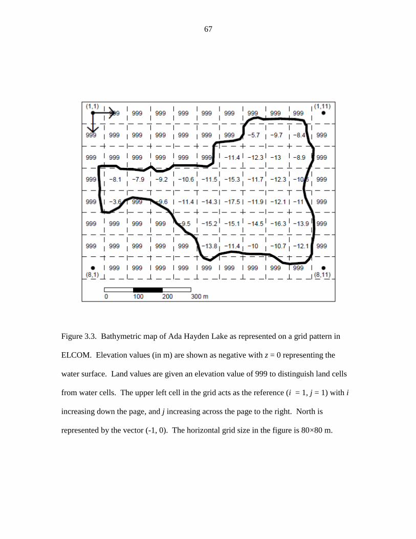
67
Figure 3.3. Bathymetric map of Ada Hayden Lake as represented on a grid pattern in
ELCOM. Elevation values (in m) are shown as negative with z = 0 representing the
water surface. Land values are given an elevation value of 999 to distinguish land cells
from water cells. The upper left cell in the grid acts as the reference (i = 1, j = 1) with i
increasing down the page, and j increasing across the page to the right. North is
represented by the vector (-1, 0). The horizontal grid size in the figure is 80×80 m.
68
x-direction must be uniform, but it could differ from the constant grid size in the y-
direction. However, the horizontal grid size was equal in each direction for all
simulations.
The computational space–as well as the output data–is represented in (i, j, k)
space. The i, j, and k values are integer indices of a three-dimensional array. Just as in
real (x, y, z) space, (i, j, k) space also maintains the right hand rule, with non-zero,positive
integers. Therefore, k = 1 is associated with the lowest cell layer (the lake
bottom). The user provides the bathymetry data by designating the vertical distance
measured from the z = 0 baseline for each cell. ELCOM differs from other data storage
programs in that the origin is located in the upper-left corner, as opposed to the
conventional mirror-image storage with the origin at the lower-left corner.
There are two cell qualifiers to keep in mind when setting up the bathymetry.dat
file: land values and open values. A land value should be given to each cell which does
not initially contain water. An open value is to be used when simulating an estuary or
coastal ocean environment where the area is open to the ocean or similar body of water.
Each cell within the bathymetry.dat file must contain one of three values: i) a vertical
distance (m) corresponding to the basin depth, ii) a land value, or iii) an open value. The
land value is typically listed as 999, and an open value is 888. These values do not
correspond to 999 and 888 m above the baseline level; they merely signal that ELCOM
will recognize these designated values and reserve these cells as land values and open
values, respectively.
ELCOM‘s pre-processor code requires the number of rows in the x-direction, the
number of columns in the y-direction, and the number of vertical layers in the z-direction.
69
If there is insufficient memory to process the bathymetry data, the initial number of grid
cells can be estimated by providing a value for the keyword n_max. Otherwise, setting
n_max = 0 will result with the code initiating a grid size of x_rows by y_columns by
z_layers, and reducing the size by removing unused cells designated as land values. For
all simulations, no estimates were made for the number of grid cells; minimum grid sizes
were selected such that sufficient memory was available for processing.
Horizontal grid size is given by x_grid_size and y_grid_size, respectively, while
the vertical grid size is given by the dz variable. ELCOM allows for changes in the
vertical grid size by designating a structure of horizontal layers which can vary with
depth. The layer thicknesses are entered in descending values from the top of the domain
in a vector array. However, the selection of the vertical spacing does have some
implications. Although any manner of vertical grid resolution is allowed, the simulation
will provide the best accuracy using a grid of uniform thickness or one in which the
changes in dz are gradual (Hodges and Dallimore, 2007). Therefore, each simulation was
modeled using a uniform vertical grid size. The maximum depth of the lake was divided
by dz and rounded up to not cut off part of the water column. An additional layer was
added when required (for small values of dz) to account for changes in water level and to
reproduce surface waves. At every model time step, ELCOM updates whether a cell is
wet (contains water) or dry (does not contain water). In this way, there were no adverse
effects from adding an additional vertical layer.
As wind forcing on the surface requires a direction, the direction of the north
arrow is also required. Because of ELCOM‘s convention when defining the origin, a
standard ―north up‖ data set has a north vector of (-1, 0). The latitude, longitude, and
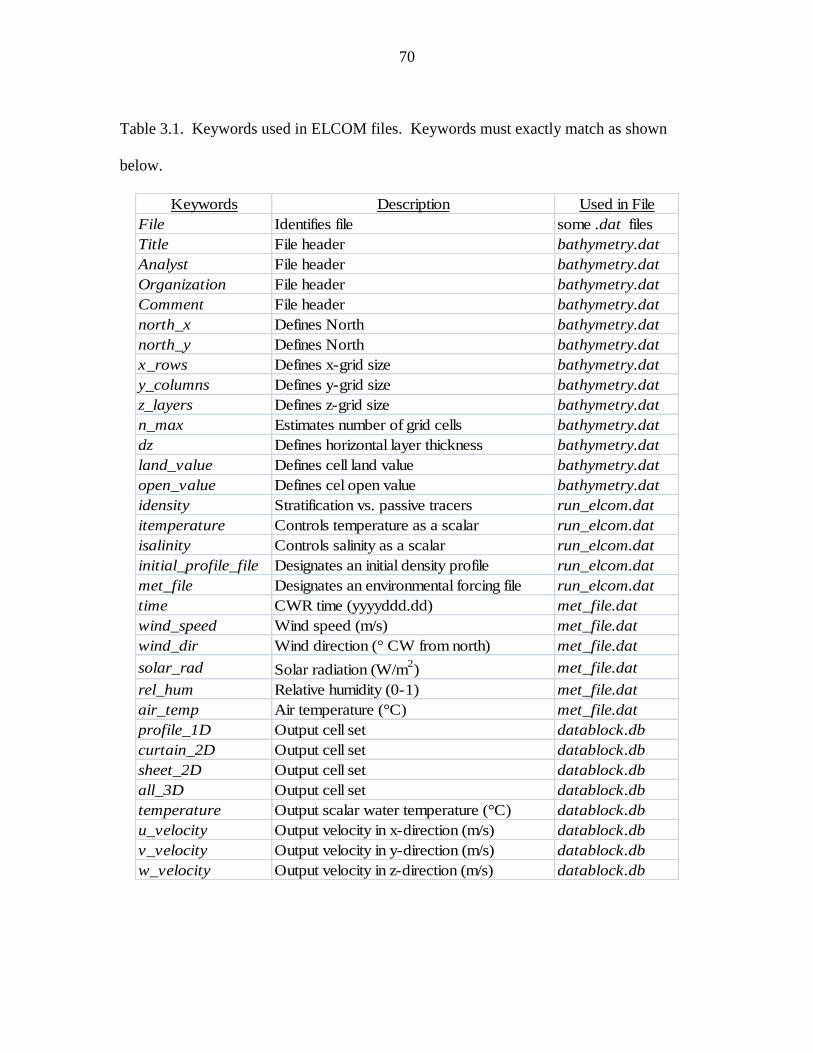
70
Table 3.1. Keywords used in ELCOM files. Keywords must exactly match as shown
below.
Keywords Description Used in File
File Identifies file some .dat files
Title File header bathymetry.dat
Analyst File header bathymetry.dat
Organization File header bathymetry.dat
Comment File header bathymetry.dat
north_x Defines North bathymetry.dat
north_y Defines North bathymetry.dat
x_rows Defines x-grid size bathymetry.dat
y_columns Defines y-grid size bathymetry.dat
z_layers Defines z-grid size bathymetry.dat
n_max Estimates number of grid cells bathymetry.dat
dz Defines horizontal layer thickness bathymetry.dat
land_value Defines cell land value bathymetry.dat
open_value Defines cel open value bathymetry.dat
idensity Stratification vs. passive tracers run_elcom.dat
itemperature Controls temperature as a scalar run_elcom.dat
isalinity Controls salinity as a scalar run_elcom.dat
initial_profile_file Designates an initial density profile run_elcom.dat
met_file Designates an environmental forcing file run_elcom.dat
time CWR time (yyyyddd.dd) met_file.dat
wind_speed Wind speed (m/s) met_file.dat
wind_dir Wind direction (° CW from north) met_file.dat
solar_rad Solar radiation (W/m2) met_file.dat
rel_hum Relative humidity (0-1) met_file.dat
air_temp Air temperature (°C) met_file.dat
profile_1D Output cell set datablock.db
curtain_2D Output cell set datablock.db
sheet_2D Output cell set datablock.db
all_3D Output cell set datablock.db
temperature Output scalar water temperature (°C) datablock.db
u_velocity Output velocity in x-direction (m/s) datablock.db
v_velocity Output velocity in y-direction (m/s) datablock.db
w_velocity Output velocity in z-direction (m/s) datablock.db

71
Table 3.2. ELCOM files. Exact filenames are not required as shown, descriptive names
were simply chosen for clarity.
Files Presence Used by: Generated by:
bathymetry.dat required pre_elcom.exe User
bc.dat required pre_elcom.exe User
update.dat optional pre_elcom.exe User
run_pre.dat required pre_elcom.exe User
DataOut.txt output pre_elcom.exe
sparsedata.unf output elcom.exe pre_elcom.exe
usedata.unf output elcom.exe pre_elcom.exe
initial_profile.dat required elcom.exe User
boundary_condition.dat required elcom.exe User
datablock.db required elcom.exe User
run_elcom.dat required elcom.exe User
elcom_out.unf output dbconv.exe elcom.exe
dataconvert.dat required dbconv.exe User
convert_out.nc output dbconv.exe
altitude of the simulation can be specified, where values reference the origin cell. The
latitude is used to provide Coriolis forces, while the longitude and altitude do not enter
into any calculations. Latitudes in the northern hemisphere are positive, and simulations
occurring in the southern hemisphere will use negative latitude values.
The bathymetry.dat file requires a file header for proper processing. The first
non-comment line of the file must begin with the keyword File, followed by the name of
the bathymetry file (e.g. bathymetry.dat). The next four lines are reserved for a
description of the file and are read by ELCOM in keyword; ‘string’ notation. There are
four keywords: Title, Analyst, Organization, and Comment. The string associated with
each keyword must contain non-null characters and enclosed in single quotation marks.

72
If the string is left empty, the pre-processer will crash. The file must have only one
Comment line. The information provided in the file header will be printed to the output
file and at the beginning of the start of the simulation run. The bathymetry section must
be completely filled with data; there can be no missing elevation values.
Bathymetry data for Ada Hayden Lake and West Okoboji Lake were provided in
two different forms. Data for Ada Hayden Lake were obtained by combining depth
measurements from a Lowrance 520C 200 kHz sonar with 10 cm resolution and a
WAAS-enabled hemisphere R100 GPS unit with 60 cm resolution, each sampling at 0.25
Hz frequency using LabVIEW. Depth and position data were linearly interpolated to
provide a suitable grid for ELCOM. Data for West Okoboji Lake were obtained through
the Iowa Department of Natural Resources with a horizontal resolution of 15 m.
The horizontal and vertical grid resolutions were modified for each simulation
event. For a simulation, the horizontal and vertical measurements were linearly
interpolated onto a suitable grid size. The model grid sizes and time steps were varied for
each particular event, with changes being made in the horizontal (Δx) and vertical (Δz)
grid size, as well as the model time step (Δt). After Hodges et al. (2006), model
simulations were run at efficient time steps with the Courant-Friedrichs-Lewy (CFL)
number held fixed at 1/3, where the CFL number is applied to baroclinic motions as
1
3n
tCFL c
x
(3.1)

73
where nc is the phase speed of the V1H1 internal wave. The V1 wave was selected as it
propagates with the highest phase speed. Therefore, the CFL number will be highest for
V1H1 seiche, assuring stability for seiches with a higher number of vertical modes. The
vertical grid size does not enter (3.1), leaving a relationship between x and t based on
the phase speed of an internal wave. Therefore, given a horizontal model grid size and
phase speed, the model time step was determined explicitly from (3.1).
Pre-Processing
The pre-processing code run_elcom.exe is paired with a run_pre.dat file which
contains the names and locations of required bathymetry files. ELCOM uses four input
files and three output files in the pre-processing code. The input files consist of i) a
bathymetry file bathymetry.dat, ii) a boundary condition file bc.dat, iii) a boundary
condition update file update.dat, and iv) a data file run_pre.dat which is associated with
the pre-processing code. Three input files are required for the pre-processor code:
bathymetry.dat, bc.dat, and run_pre.dat, while the update.bc file is optional. The
bathymetry file was previously discussed concerning the syntax and setup involved. The
boundary condition file designates cell sets for various conditions such as river
infow/outflow, groundwater inflows, or a bubble plume. While required, the boundary
condition file was left empty because Ada Hayden Lake and West Okoboji Lake were
modeled as closed basins. The boundary condition update file allows arbitrary
modification in scalar values (e.g., a tracer release). No tracer studies were modeled
using ELCOM; therefore, the update.dat file was not used. The file run_pre.dat is
74
required for the pre-processing code and contains names and locations of input/output
files used by pre_elcom.exe.
Output directories should correspond to the infiles directory used by the
processing code. The setup of the processing code will be discussed in a later section.
The output files for the pre-processing code consist of one text file and two unformatted
files: i) data output text file, ii) usedata.unf, and iii) sparsedata.unf. The data output text
file contains pre-processing results and is generally not important for the model
simulation. However, the usedata.unf and sparsedata.unf files are required for elcom.exe
processing as they contain bathymetry data given by the pre-processing code. The
directory associated with the output of the pre-processing code must coordinate with
specified directories in the main processing code. Once all pre-processing files are
complete and placed in locations designated by run_pre.dat, the next step is to run the
pre-processing code. Running the pre-processing code is accomplished by executing
pre_elcom.exe at the command line.
Temperature Profiles
The initial conditions for the temperature structure in the lake can be specified
through the use of vertical profiles. Density stratification in ELCOM can be through salt,
temperature, or both, and is controlled using the keywords idensity in conjunction with
itemperature and isalinity. Setting idensity = 1 enables density stratification, while
setting idensity = 0 will allow for temperature and salinity to be treated as passive tracers
(i.e., eliminating the density term from the momentum equations). Initial conditions can

75
be specified with any number of input files identified by ELCOM using the keyword
initial_profile_file. Because all simulations were for freshwater lakes and stratification is
attributed solely to temperature, itemperature and idensity were each set to1, while
isalinity was set to 0. Multiple input files were used to provide initial conditions, where
these files were generated using field data from the thermistor chains.
The vertical profile input files require a format consisting of four header lines
followed by columns of data. The first line in the file header includes the number of data
sets (columns) in the initial profile, not including the depth column. The second line in
the file header provides the number of rows containing data. The third header line
contains the horizontal location of the profile, given in the (i, j) coordinate system. The
fourth line contains keywords which correspond to the data provided in each of the
columns. Depth values are required in the first column, while other data is required to be
an ELCOM valid transportable scalar (i.e., salinity, water temperature, or a tracer
concentration). Therefore, the first keyword in the fourth line must be depth followed by
wtr_temp for the case of temperature-stratification.
The depth values in the first column started at zero and increased monotonically
(depth is defined as vertically downward), while the temperature values in the second
column were determined from field measurements. ELCOM linearly interpolates the
initial data given in the vertical profile files onto the grid given by the bathymetry data.
Horizontal interpolation is done for multiple profiles using the inverse distance weighting
method, given by Hodges and Dallimore (2007):
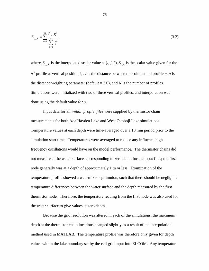
76
,
, ,
1
1
Nn k n
i j k Nn
m
m
S rS
r
(3.2)
where , ,i j kS is the interpolated scalar value at (i, j, k),
,n kS is the scalar value given for the
nth
profile at vertical position k, rn is the distance between the column and profile n, α is
the distance weighting parameter (default = 2.0), and N is the number of profiles.
Simulations were initialized with two or three vertical profiles, and interpolation was
done using the default value for α.
Input data for all initial_profile_files were supplied by thermistor chain
measurements for both Ada Hayden Lake and West Okoboji Lake simulations.
Temperature values at each depth were time-averaged over a 10 min period prior to the
simulation start time. Temperatures were averaged to reduce any influence high
frequency oscillations would have on the model performance. The thermistor chains did
not measure at the water surface, corresponding to zero depth for the input files; the first
node generally was at a depth of approximately 1 m or less. Examination of the
temperature profile showed a well-mixed epilimnion, such that there should be negligible
temperature differences between the water surface and the depth measured by the first
thermistor node. Therefore, the temperature reading from the first node was also used for
the water surface to give values at zero depth.
Because the grid resolution was altered in each of the simulations, the maximum
depth at the thermistor chain locations changed slightly as a result of the interpolation
method used in MATLAB. The temperature profile was therefore only given for depth
values within the lake boundary set by the cell grid input into ELCOM. Any temperature
77
measurements at depths greater than the equivalent grid location were not input into the
model. As the grid resolution was reduced (i.e., the horizontal spacing increased), the
bottom boundary at each cell was interpolated over more points. This interpolation
resulted in maximum depths that would decrease with increased horizontal grid sizes.
Environmental Forcing
ELCOM incorporates environmental forcing conditions by data given in temporal
boundary condition files (met.dat). These one-dimensional files designate environmental
conditions at a particular point, if multiple files are used, or for the entire free surface in
the case of one boundary file. ELCOM recognizes many data types within a boundary
condition file and the data supplied are required for each instant in time. For all
simulations, five data types (other than time) were input into ELCOM: wind speed, wind
direction, relative humidity, solar radiation, and air temperature. Simulations at Ada
Hayden Lake used field measurements from the LDS for all data types. However, the
temperature probe malfunctioned while in the field during deployment at West Okoboji
Lake. The Iowa Great Lakes Water Safety Council has a weather station located at the
Gull Point State Park which was used to supply air temperature values at 15 min
intervals. These 15 min values were linearly interpolated to correspond with the
sampling frequency of the LDS to provide accurate temperature values.
The boundary condition file requires a file header designating the number of data
sets and the type of data used. The first line contains the number of data sets within the
file not including the time values. The second line should contain the number 0, which
78
indicates CWR time format is being used. The third line requires integer values for each
data column designating the location of the boundary condition file. For boundary
conditions applied to the entire surface, these integer values should all be set to 0. The
fourth line contains keywords that describe the data set in each column. The first
keyword should be time, as time values are required in the first column. See Table 3.1
for a list of keywords and the appropriate units.
The data in the boundary condition file are organized into columns, with the first
column containing time in CWR format (yyyyddd.dd). Each successive column contains
data for a respective data type, and each row contains data values for the respective time
step. The time interval used in the boundary condition file is not required to correspond
with the model time step; ELCOM will linearly interpolate the input data values onto a
suitable time grid. Within the data columns, missing data values will cause the code to
crash; each row must have the appropriate number of data values to correspond with the
number of columns.
Designating Model Output, Running Simulations, and Post-Processing
ELCOM provides a number of data output options. Output information is
designated in a datablock.db file, which is organized into series of blocks. The first four
lines of the datablock.db file are the datablock descriptions, including the ELCOM
version number, the number of output groups, and the number of output sets. Output
groups identify a group of data to be output, such as temperature, velocities, etc. The
output sets specify points (cells) at which data are to be output. Output cell sets can be

79
either one-dimensional profiles, a continuous series of columns (curtains), a horizontal
series of cells (sheets), or the entire domain. Table 3.1 contains the keywords associated
with each type of output cell set types and scalar types. There are 11 lines in each group
description and 16 lines for each set description. As the cell set type changes, values will
change for ‗sheet type‘, ‗sheet calc‘, ‗sheet value‘, and the ‗cell location‘ lines. For a
complete description of the options and requirements for a datablock file, see Hodges and
Dallimore (2007).
ELCOM is executed at the command line by typing elcom.exe in the appropriate
directory. ELCOM will send monitoring information to the command line, which will
show any errors during a simulation. Once the model is complete, post-processing of the
elcom_out.unf files is required. The post-processing code dbconv.exe converts the model
output into NetCDF convert_out.nc files which are compatible with MATLAB. The
post-processing code requires .dat files which specify.unf filenames and locations, as well
as the name and location of the converted .nc file. Running the post-processing code is
done by typing dbconv.exe at the command line in the unf directory of ELCOM.
Description of Numerical Methods
ELCOM‘s numerical scheme is adapted from the TRIM approach (Casulli and
Cheng, 1992). The approach uses an Arakawa C-grid stencil, which defines velocities on
cell faces, while the free surface height and scalar concentrations are defined on cell
centers. ELCOM uses a semi-implicit method where the water surface gradient, the
velocity in the free surface equation, and the vertical mixing terms are discretized

80
implicitly. The advective, Coriolis, and horizontal viscosity terms in the momentum
equations are discretized explicitly. A brief description of the numerical method used by
ELCOM will be presented. For more details, see Casulli and Cheng (1992), Hodges et al.
(2000), and Hodges and Dallimore (2006).
Momentum Discretization
ELCOM solves the velocity field in a manner similar to the TRIM approach given
by Casulli and Cheng (1992), with the addition of a vertical mixing model and the use of
a hybrid linear/quadratic Eulerian-Lagrangian method. The momentum equations in the
x and y directions are
1
1 1 1
1/2, 1/2, 1/2, 1, ,
n n n n n
i j i j i j i j i j
tU A G g
x
(3.3)
1
1 1 1
, 1/2 , 1/2 , 1/2 , 1 ,
n n n n n
i j i j i j i j i j
tV A G g
y
(3.4)
where U and V are matrices containing the velocities at location (i, j) and is the free
surface height. Subscripts , ,i j k refer to cell locations and superscript n refers to time.
G is an explicit source term and A is a matrix defined as
1 1 1
2 2
2 2
1 1 1
0 0
0 0
0 0
n k n
n n n
n n
b c
a b c
A a b
b c
a b
(3.5)

81
where the k terms are set by ELCOM to correspond to boundary conditions (e.g., no-
slip, free-slip, Neumann, etc.), while the a, b, and c terms are given by
k k k kb a z c (3.6)
3
1/2
k
k
ta
z
(3.7)
3
1/2
k
k
tc
z
(3.8)
where 3 is the viscosity in the z-direction, t is the model time step, and z is the
vertical grid size. The source terms in G are given by
1/2, 1/2, 1/2, 1/2,1/2, 1/2,
n
i j i j i j x y i ji j i j
G I U t C D U D U fV
(3.9)
, 1/2 , 1/2 , 1/2 , 1/2, 1/2 , 1/2
n
i j i j i j x y i ji j i j
G I V t C D V D V fU
(3.10)
where the I operator represents advective discretization, C represents baroclinic
discretization, and ,x yD represents horizontal turbulent diffusion discretization in the x
and y direction, respectively. ELCOM uses a vertical mixing model to account for
vertical diffusion, where the mixing operator M is defined as

82
, , , ,
n
i j k i j kU M U (3.11)
ELCOM uses a second-order stencil for the discretization of the horizontal diffusive
terms, the diffusive term in the x-direction is given as
, , 1, , , , 1, ,22n n n n
x i j k i j k i j k i j kD S S S Sx
(3.12)
where S is any scalar. The baroclinic discretization term C is defined as
' '
1/2, , 1, , , ,
0
F Fn
i j k i j m i j m
m k m k
gC
x
where is the density perturbation from the reference value, and k F is the cell
containing the free surface. The free surface discretization is given by
1 1 1
, ,
T Tn n n n n n
i j i j x y
t tZ U Z V
x y
(3.13)
where Z is a vector containing the vertical grid size, and the operators x and y
indicate discrete differences, such that 1/2 1/2x i iS S S .
The TRIM method (Casulli and Cheng, 1992) uses a linear Eulerian-Lagrangian
method for the discretization of the advective and viscous terms. ELCOM uses a hybrid
method which is a combination of the linear Eulerian-Lagrangian method for 2CFL ,
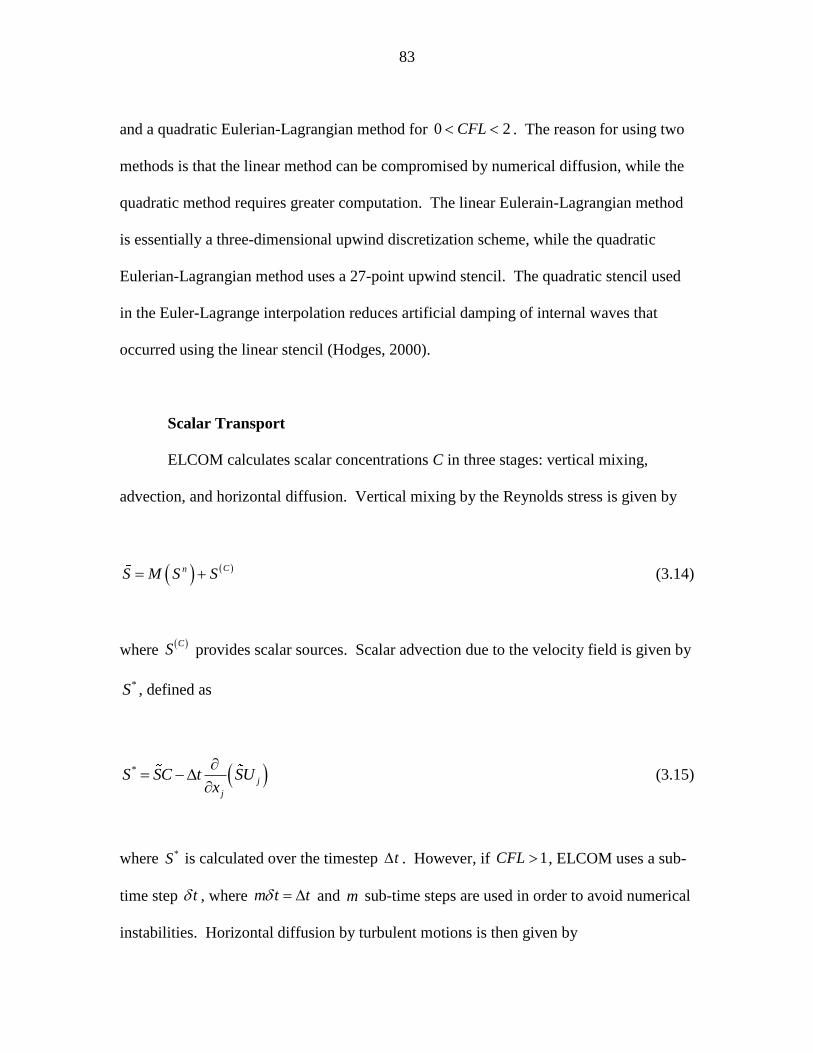
83
and a quadratic Eulerian-Lagrangian method for 0 2CFL . The reason for using two
methods is that the linear method can be compromised by numerical diffusion, while the
quadratic method requires greater computation. The linear Eulerain-Lagrangian method
is essentially a three-dimensional upwind discretization scheme, while the quadratic
Eulerian-Lagrangian method uses a 27-point upwind stencil. The quadratic stencil used
in the Euler-Lagrange interpolation reduces artificial damping of internal waves that
occurred using the linear stencil (Hodges, 2000).
Scalar Transport
ELCOM calculates scalar concentrations C in three stages: vertical mixing,
advection, and horizontal diffusion. Vertical mixing by the Reynolds stress is given by
CnS M S S (3.14)
where C
S provides scalar sources. Scalar advection due to the velocity field is given by
*S , defined as
*
j
j
S SC t SUx
(3.15)
where *S is calculated over the timestep t . However, if 1CFL , ELCOM uses a sub-
time step t , where m t t and m sub-time steps are used in order to avoid numerical
instabilities. Horizontal diffusion by turbulent motions is then given by
84
*
1 * 2n SS S O t
x x
(3.16)
where 2O t is a truncation error which is second order accurate in time. ELCOM
uses the Universal Limiter for Transient Interpolation Modeling of the Advective
Transport Equations Quadratic Upstream Interpolation for Convective Kinematics
(ULTIMATE QUICKEST) method (Leonard, 1991) for the interpolation of scalar
concentrations from the cell center (where they are defined) to cell faces for use of
discrete difference operators x and y .
Mixing Model
The vertical mixing model accounts for vertical diffusion in the model, while
horizontal diffusion is calculated using a finite-difference approach. The vertical mixing
model in ELCOM uses a mixed layer approach, as opposed to the traditional method of
using differential equations coupling layer thickness, entrainment rates, and heat transfer.
ELCOM models the vertical Reynolds stress terms in the momentum and transport
equations three-dimensionally, expanding on previous one-dimensional models (e.g.,
Imberger and Patterson, 1981; Spigel et al., 1986; Imberger and Patterson, 1990). The
mixed-layer approach dynamically defines a ―mixed layer‖ as a vertical set of cells
sharing the same density, scalar concentrations, and grid-scale velocity (Hodges, 2000).
The mixed layer method showed a bias for downward entrainment and mixing, as the
model is applied down the water column from the water surface to the lake bottom
(Hodges et al., 2000).
85
A mixing time step is broken into 12 steps: 1) calculate wind energy input, 2)
calculate bottom energy input from the turbulent bottom boundary layer, 3) for each
column, cycle vertically from the surface to the bottom cell, 4) calculate generation of
turbulent kinetic energy (TKE) by shear, 5) calculate energy required for mixing, 6)
calculate total energy available if two cells mix completely, 7) calculate time for
complete mixing, 8) if unstable, calculate time estimate based on convective overturn, 9)
calculate mixing fraction, 10) if sufficient energy, mix the cells, 11) end cycle at bottom
cell, and 12) dissipate excess mixing energy.
Data Analysis of Field Work and Model Results
Dimensionless variables such as the Wedderburn number W and the Lake
number NL integrate factors such as stratification, basin size, and forcing conditions into
a single estimate. When considering forcing conditions, it is important to accurately
account for the transfer of momentum (or energy) from wind shear to internal lake
dynamics as part of the energy flux path as described by Imberger (1998). For seasonal
field measurements, Stevens & Lawrence (1997) demonstrated that energy transferred at
frequencies greater than 4 / iT cannot affect baroclinic motions (where iT is the period for
the ViH1 mode seiche), but instead affects surface layer circulation, contributes to
turbulent kinetic energy, or is immediately dissipated. Filtering attenuates peaks in the
velocity, but it is required for wind events that are not constant in magnitude (Stevens &
Lawrence, 1997). Therefore, all wind data were filtered using a fourth order Butterworth

86
filter with a cutoff frequency corresponding to one-quarter of the period for the V1H1
internal wave when calculating W and NL .
To quantify model performance and compare simulations at different resolutions,
three physical attributes were evaluated between field observations and model output: i)
the frequencies of internal motions, ii) the retention of the temperature structure under
forcing conditions, and iii) internal wave amplitudes. The first attribute will be used
primarily to indicate the model‘s ability to reproduce internal motions across a wide
range of frequencies. Because ELCOM is a hydrostatic model, nonlinear effects (i.e.,
non-hydrostatic pressures) associated with higher frequency motions cannot be physically
represented by the model. The second point is important as it can indicate whether
excessive numerical diffusion is acting to erode the thermocline and will therefore help to
quantify numerical error in the model. The third item aims at addressing whether equal
forcing conditions given to ELCOM will reproduce internal motions comparable to field
observations. Additionally, a nondimensional number known as the Willmott skill will
be used to quantify model predictions.
Hydrostatic models have shown to be able to reproduce basin-scale motions, but
they are unable to resolve high-frequency motions due to restrictions on grid cell sizes
(e.g., Hodges et al., 2000; Gomez-Giraldo et al., 2006; Botelho and Imberger, 2007;
Yeates et al., 2008). Once the isotherm displacements are calculated at the thermistor
chains, Welch‘s periodogram method can used to calculate the spectral density of an
isotherm‘s displacement in frequency space. When computing power spectra, standard
default methods given using the MATLAB build-in function pwelch were used. Equal
weighting was given to each time measurement (segment), and a 50% overlap was used
87
between segments. The fast Fourier transform was determined as the larger of either the
length of the data segment or 256. Power spectra can be created for each isotherm and at
each thermistor chain, where the power spectrum gives the power of the signal at a
particular frequency. In the case of periodic motions, peaks in the power spectra
typically correlate with seiching mode frequencies.
Normalized Potential Energy
The potential energy in the water column is calculated to assess the model‘s
ability to retain the thermocline‘s temperature structure over a simulation. The advantage
to this approach is that the potential energy does not rely upon selecting a single isotherm
to represent the entire time series (Antenucci et al., 2000). Winters et al. (1995) defined
the potential energy within a fluid using a volume integral; however, here the potential
energy is evaluated in the water column as opposed to the entire water body. The
potential energy PE (per unit area) is defined as
0
( ) ,H
Pz
E t g z t zdz (3.17)
where 0z is the elevation of the lake bottom, and z is defined as positive upwards. A
time-series of potential energy is calculated from both field data and model output.
However, values for potential energy are typically O(106) kg/s
2 and they only by vary
O(102) kg/s
2 ; therefore, the change in potential energy from a reference value was
88
evaluated. Also, by evaluating changes in potential energy as opposed to the total value,
results can be obtained which aim to evaluate the model‘s ability to reproduce changes in
the temperature structure over a set time period.
The reference value was defined using the difference between the initial and
minimum potential energy values calculated from field measurements. This definition
was made because of the difference in magnitudes of potential energy values across
simulations of different vertical grid sizes. The potential energy reference value ,0PE for
each model run is then defined as
,0 ,model ,field ,field0 0 minP P P PE E E E (3.18)
where ,model 0PE is the initial potential energy value calculated using model output and
the value in brackets is the reference potential energy difference based on field data
,fieldPE . Initial potential energy estimates based on model results were within 10% of
the values calculated from field observations. While this difference is important, the
effects of numerical error in the model affect the change in potential energy of the
simulation period. The fluctuations in potential energy are then found by subtracting the
reference value from the model results
,model ,0P P PE E E (3.19)
89
To compare the potential energy values across different simulations, a time-
integrated value for potential energy is calculated. By integrating PE over time, a
single potential energy value can be obtained for each model run. The time-integrated
potential energy values calculated from model results are normalized by the value
obtained from the field data to give a dimensionless value for potential energy PE ,
defined as
,field ,fieldmin
P
P
P P
E dtE
E E dt
(3.20)
The advantage to using PE is that results are easily analyzed. PE > 1 indicates a higher
center of mass, caused by either numerical diffusion or the model overestimating mixing.
PE < 1 would be the result of isotherms deepening in the model, lowering the center of
mass.
Normalized Kinetic Energy
To evaluate the model‘s ability to reproduce internal wave amplitudes, kinetic
energy is calculated based on field data and model output. Here, kinetic energy will be
based on the vertical velocity w , omitting horizontal velocities u and v . The reason for
defining kinetic energy using only the vertical velocity lies in the difficulty in estimating
horizontal velocities from thermistor chain measurements. ELCOM can output values for
90
the velocity vector , ,u v w directly, but estimating w based on thermistor chain
measurements is done by tracking isotherm movements. Isotherm positions are found by
linearly interpolating temperature data from the thermistor chains. Because the top and
bottom of the water column are less stratified than the metalimnion (it is not uncommon
for the epilimnion to be completely mixed), it can be difficult to achieve accurate
isotherm depths using a linear interpolation method in these regions. Therefore, the
analysis is limited to the thermocline region.
Once the isotherm positions are determined, is defined simply as the time
derivative. The depth-integrated kinetic energy is defined after Winters et al. (1995) as
2
1
20
2
z
Kz
E t w t
(3.21)
where 0 is a reference density, and the bounds 1z and 2z are defined as the top and
bottom of the metalimnion, respectively. When comparing field observations to model
output, a similar metalimnion thickness—or constant values for 1z and 2z —were used.
As in the expression for potential energy, is defined as positive upwards. The time
series of kinetic energy values are analyzed similar to potential energy by integrating in
time and normalizing model results by field data estimates to provide a dimensionless
value of kinetic energy KE , defined as
91
2
1
2
1
2
model
2
field
z
z
K z
z
w dzdtE
w dzdt
(3.22)
where modelw is the vertical velocity given by ELCOM and fieldw is the vertical velocity
based on isotherm depths from field data. Both velocities are functions of depth and
time.
Willmott Skill Number
Additionally, a nondimensional number has been proposed which compares a
physical parameter between field and model results, known as the Willmott skill WS
(Willmott and Wicks, 1980; Willmott, 1981), defined as
2
model field
2
model field field field
X XWS
X X X X
(3.23)
where modelX is a parameter based on model results, fieldX is a corresponding parameter
from field observations with time average fieldX . WS is a nondimensional number
ranging from zero to one, where a value of one indicates perfect agreement and zero
yields complete disagreement (Warner et al., 2005). The Willmott skill number can
therefore be used to compare results from different parameters in the same simulation or
different models directly with one another.
92
Willmott (1982) evaluated evapotranspiration models and found WS values of
0.82 and 0.90 using the Makkink and Blaney-Criddle models, respectively. Warner et al.
(2005) estimated the performance of the Regional Ocean Modeling System (ROMS)
using the Willmott skill number and found WS values of 0.85 and 0.95 for sea level at
two different locations in a model, 0.92 for depth-averaged velocities, and 0.85 for
salinity concentrations. Wilkin (2006) used ROMS to model ocean circulation near Cape
Cod, Massachusetts and found WS values between 0.2 and 0.8 in comparing observed
and modeled temperatures at different instrument locations. Liu et al. (2009) used
ROMS in the River Influence on Shelf Ecosystem (RISE) project at the mouth of the
Columbia River in Washington and calculated WS numbers for velocities, temperatures,
and salinities in the top and bottom of the water column and near the river discharge
(nearfield) and offshore (farfield). The regions were combined by averaging WS values,
giving average values ranging from 0.48 to 0.97. For the model analysis of this work,
Willmott skill numbers were calculated using the depth of an isotherm near the center of
the metalimnion.
Summary
Chapter 3 identified the methods for conducting field observations and the
procedure for implementing a three-dimensional hydrostatic model, and it presented
dimensionless variables used to quantify and assess model performance. Instrument
locations have been identified for three years of field work in two lakes. Also, sampling
strategy and explanations involved when planning field studies were presented. Steps

93
were presented which outline the necessary elements for a successful simulation using
ELCOM. The model grid sizes and time steps used for individual model runs, as well as
the details of a particular simulation, will be presented in Chapter 4 following field
analysis.
Two dimensionless energy variables have been defined based on potential and
kinetic energy. These variables can be used to quantify model performance in terms of
retaining the temperature structure and reproducing internal wave amplitudes. A perfect
model simulation would return values of one for each of the variables. Also, a
nondimensional number has been described which can be used to compare the agreement
between model predictions and field observations. However, it will be shown in Chapter
4 that results will vary considerably from a perfect solution.

94
CHAPTER 4: RESULTS AND DISCUSSION
Introduction
Chapter 4 discusses the results from the field work and numerical modeling.
Field results will be discussed in terms of their significance for generating basin-scale
internal motions. Additionally, dimensionless energy variables developed in Chapter 3
will show the applicability of three-dimensional hydrostatic modeling. Model results will
be presented, analyzed, and model performance will be quantified using dimensionless
energy variables defined in Chapter 3.
Field Results
The conducted field work consisted of measuring temperature stratification by
deploying several thermistor chains at various locations across the lake. Additionally,
environmental forcing conditions were measured to determine the effects forcing has on
the internal motions of a lake. Forcing parameters include wind speed and direction,
solar radiation, air temperature, and relative humidity. The measured conditions will be
analyzed in terms of the likely mechanisms involved in the energy flux path and the
ability of a hydrostatic model to capture these mechanisms.

95
Ada Hayden Lake
Wind and temperature data measured from the Lake Diagnostic System (LDS)
from 17 July to 1 October are shown in Figure 4.1. There are several days which
experienced high winds (between 10 and 15 m/s), most notably the 18th
and 26th
of July,
the 28th
of August, and the 18th
of September. More sustained wind gusts of lesser
magnitudes (between 5 and 10 m/s) were experienced the 5th
and 26-27th
of August.
Strong gusts tend to originate from the north, while calmer, more sustained winds tend to
emerge from the southwest or southeast (Fig. 4.1(b)). To relate the wind forcing to the
lake‘s stratification, the Lake number is shown to vary considerably throughout the
summer from low values approaching O(1) to higher values exceeding O(102).
Measurements are shown from mid-July through the end of September, depicting
the change in stratification during the summer months. As shown in Fig 4.1d, the
isotherm depths begin to increase until 16 September, when air temperature (not shown)
begins to decrease, halting the mixed-layer deepening. Only isotherms which are present
throughout the depicted time are shown to relate internal response to external forcing.
The strong stratification during the summer months leads to small isotherm
displacements under observed wind forcing.
Figure 4.2 shows field results from Ada Hayden Lake in 2008, encompassing
measured conditions between 22 July and 1 October. In general, conditions in 2008
depict comparable wind conditions to those observed in 2007. Similar to situations
experienced in 2007, high winds could be considered exceeding 10 m/s, while more
sustained winds of interest also typically exceed 5 m/s. High wind occurred on 27 and 29

96
Figure 4.1. Field results from Ada Hayden Lake in 2007, as measured by the LDS: (a)
wind speed measured at 2.40 m above the water surface, (b) wind direction (°) measured
clockwise from north (0°), (c) Lake number calculated using filtered wind speed and
temperature data from the LDS, (d) contour plot showing isotherm depths for even
isotherms between 8 and 28°C.

97
Figure 4.2. Field results from Ada Hayden Lake in 2008, as measured by the LDS: (a)
wind velocity (m/s) measured at 2.10 m above the water surface, (b) wind direction (°)
measured clockwise from north (0°), (c) Lake number calculated using filtered wind
speed and temperature data from the LDS, (d) contour plot showing isotherm depths for
even isotherms between 10 and 28°C.

98
July, 14 August, and 23 and 29 September, with corresponding low Lake numbers and
large internal isotherm movement. More sustained conditions of lower magnitude are
more frequent and can be seen on 23 and 31 July, 4 and 22 August, and 2, 14, and 19
September. These times are shown to experience moderate Lake numbers but typically
not dropping much below a value of 10. Similar to the high-wind events, lower-
magnitude and longer-duration winds can also be seen to result in isotherm displacement
but not of the same magnitude. As in 2007, stronger winds tend to come from the
northwest to north, and calmer winds are more often seen emanating from the southeast
(Fig. 4.2b). The isotherm depths slowly increased until 17 September (Fig. 4.2d), similar
to conditions in 2007.
Figure 4.3 shows the temperature profile as measured by the LDS for the same
time periods in both 2007 and 2008, corresponding to Figures 4.1 and 4.2. The behavior
of the thermal structure over the summer months in the time period shown in Figure 4.3
is quite similar between successive years. For both years, the initial surface mixed layer
is approximately 3 m deep, while the metalimnion extends to a depth of approximately 8-
9 m. The thermal structures on 30 September also show similarities. The base of the
mixed layer deepened to approximately 6 m and the temperature in the epilimnion cooled
to 19-20°C.
The differences lie in the discrepancy between the temperatures in the
hypolimnion. The hypolimnion is 3-4°C warmer in 2008 as compared to 2007. Due to
the comparatively warmer conditions in the hypolimnion, coupled with similar
temperatures in the surfaced mixed-layer, there is consequently less stratification in 2008.
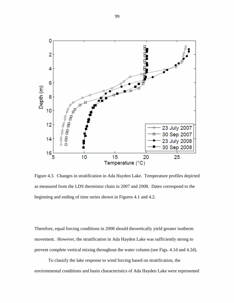
99
Figure 4.3. Changes in stratification in Ada Hayden Lake. Temperature profiles depicted
as measured from the LDS thermistor chain in 2007 and 2008. Dates correspond to the
beginning and ending of time series shown in Figures 4.1 and 4.2.
Therefore, equal forcing conditions in 2008 should theoretically yield greater isotherm
movement. However, the stratification in Ada Hayden Lake was sufficiently strong to
prevent complete vertical mixing throughout the water column (see Figs. 4.1d and 4.2d).
To classify the lake response to wind forcing based on stratification, the
environmental conditions and basin characteristics of Ada Hayden Lake were represented

100
using a two-layer model (Fig. 4.4), after Horn et al. (2001). The timescales for various
degeneration mechanisms (i.e., Kelvin-Helmholtz billows, supercritical bores, solitons)
were calculated for varying stratification assuming a density change of 3.6 kg/m3, a
thermocline thickness of 5 m, and a turbulent boundary layer thickness of 1 m. These
timescales are plotted in terms of the ratio of the amplitude of the basin-scale wave 0 to
the surface layer 1h (equivalently, the inverse of the Wedderburn number 1W ) and the
depth ratio of the surface layer to the total depth H .
Wind and temperature measurements from 2007 and 2008 were analyzed to
determine the stratification (represented by the depth ratio) 1 /h H and the lake response
1W due to wind forcing. The observed points were binned and given a percentage value
pertaining to the relative frequency of the number of occurrences in the respective bin to
the total number of occurrences (Fig. 4.4). Observed values indicate Ada Hayden Lake
experiences sufficient stratification, due to the high values of the depth ratio ranging from
0.34 to 0.5. Additionally, the high values of W show resistance of the lake to internal
movement caused by wind shear. The observed values lie exclusively within Regime 1,
and will therefore be governed by linear wave theory. Thus, the field data indicates Ada
Hayden Lake lends itself well to hydrostatic numerical models, as nonlinear steepening
and non-hydrostatic pressures do not appear to be prevalent.
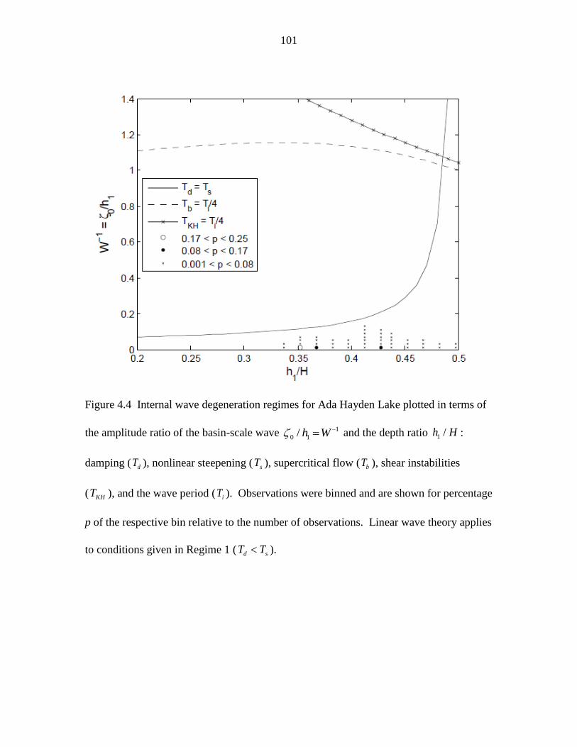
101
Figure 4.4 Internal wave degeneration regimes for Ada Hayden Lake plotted in terms of
the amplitude ratio of the basin-scale wave 1
0 1/ h W and the depth ratio 1 /h H :
damping ( dT ), nonlinear steepening ( sT ), supercritical flow ( bT ), shear instabilities
( KHT ), and the wave period ( iT ). Observations were binned and are shown for percentage
p of the respective bin relative to the number of observations. Linear wave theory applies
to conditions given in Regime 1 ( d sT T ).

102
West Okoboji Lake
Comparing results from Ada Hayden Lake to results from West Okoboji Lake
allows the effect of differences in lake size, geometry, wind forcing, and stratification to
be studied. Measurements from the LDS at West Okoboji Lake between 28 May and 23
July in 2009 are shown in Figure 4.5. Compared to field results from Ada Hayden Lake,
shown in Figures 4.1 and 4.2, West Okoboji Lake tends to experience higher velocity
winds, higher variability in stratification, and greater vertical isotherm displacement.
Wind speeds at West Okoboji Lake often exceeded 5 m/s, with sustained gusts often
exceeding 10 m/s. The wind direction was highly variable when compared to Ada
Hayden Lake, but strong wind gusts tended to originate from the west to northwest, while
calmer winds were most often seen from due north. Periods of small Lake numbers were
quite frequent from late May through June, most notably 30-31 May, and 1, 7, 19, 21, 28,
and 30 June. These periods showed significant vertical movement of the isotherms
present in the water column. Particularly, high wind events in late May forced surface
water to depths of over 20 m.
Figure 4.6 shows a histogram of NL occurrences for Ada Hayden Lake and West
Okoboji Lake. West Okoboji Lake experienced larger percentages of both small and
large Lake numbers. The only Lake number range in which Ada Hayden Lake
experienced a higher frequency of occurrence was NL = 50-100. The implications from
Figure 4.6 are this: Ada Hayden Lake was more consistent with observed lake response,
with Lake numbers typically ranging from 10 to 500, while West Okoboji Lake was more

103
Figure 4.5. Field results from West Okoboji Lake in 2009, as measured by the LDS: (a)
wind velocity (m/s) measured at 2.14 m above the water surface, (b) wind direction (°)
measured clockwise from north (0°), (c) Lake number calculated using filtered wind
speed and temperature data from the LDS, (d) contour plot showing isotherm depths for
even isotherms between 14° and 22°C.
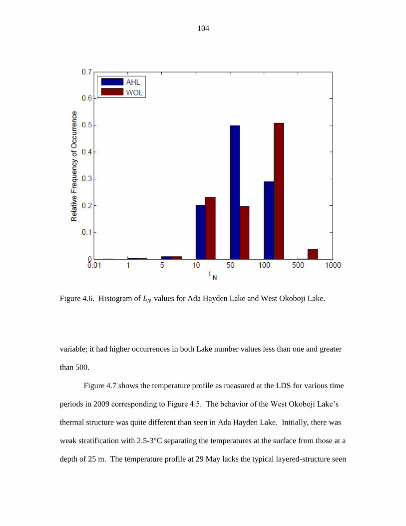
104
Figure 4.6. Histogram of values for Ada Hayden Lake and West Okoboji Lake.
variable; it had higher occurrences in both Lake number values less than one and greater
than 500.
Figure 4.7 shows the temperature profile as measured at the LDS for various time
periods in 2009 corresponding to Figure 4.5. The behavior of the West Okoboji Lake‘s
thermal structure was quite different than seen in Ada Hayden Lake. Initially, there was
weak stratification with 2.5-3°C separating the temperatures at the surface from those at a
depth of 25 m. The temperature profile at 29 May lacks the typical layered-structure seen

105
in Ada Hayden Lake (Fig.4.3) and could be considered linearly stratified. As the summer
progressed, solar radiation heated the surface water, while wind-induced mixing eroded
the stratification. The high velocity winds at West Okoboji prevented a surface mixed
layer from fully forming until mid July. At this time, the base of the mixed-layer
Figure 4.7. Changes in stratification in West Okoboji Lake. Temperature profiles
depicted as measured from the LDS thermistor chain in 2009. Changes are shown for
five periods over the course of two months.

106
extended to over 10 m, while the metalimnion extended to a depth between 16 and 19 m.
Because of weak stratification, internal motions occurred throughout the water column,
as shown in Figure 4.5d.
As previously discussed for Ada Hayden Lake, internal wave degeneration
timescales were determined for West Okoboji Lake by representing the lake as a two-
layer model to determine the lake response under different stratifications and wind events
(Fig. 4.8). The density profiles for West Okoboji Lake were more linear than seen for
Ada Hayden Lake, resulting in difficulties when using two-layer model for. However,
these time periods of near linear stratification were few and most often observed early in
the summer. Analysis was restricted to times where a two-layer structure could be
approximated. Field observations were analyzed to determine the stratification and the
lake response. The percentage and spread of the binned data is less condensed when
compared to the results from Ada Hayden Lake. West Okoboji Lake experienced varying
degrees of stratification, with depth ratios varying between 0.25 and 0.45. Additionally,
it appears the lake experienced nonlinear wave activity, as evidenced by the greater
number of occurrences in Regime 2.
While these nonlinear waves cannot be physically represented through hydrostatic
modeling, Hodges et al. (2006) proved that under forcing conditions appropriate for the
formation of nonlinear waves, numerical hydrostatic models can accurately reproduce
basin behavior for times less than the time required for the onset of steepening s ,
defined as

107
Figure 4.8 Internal wave degeneration regimes for West Okoboji Lake plotted in terms
of the amplitude ratio of the basin-scale wave 1
0 1/ h W and the depth ratio 1 /h H :
damping ( dT ), nonlinear steepening ( sT ), supercritical flow ( bT ), shear instabilities
( KHT ), and the wave period ( iT ). Observations were binned and are shown for percentage
p of the respective bin relative to the number of observations. Linear wave theory applies
to conditions given in Regime 1 ( d sT T ).
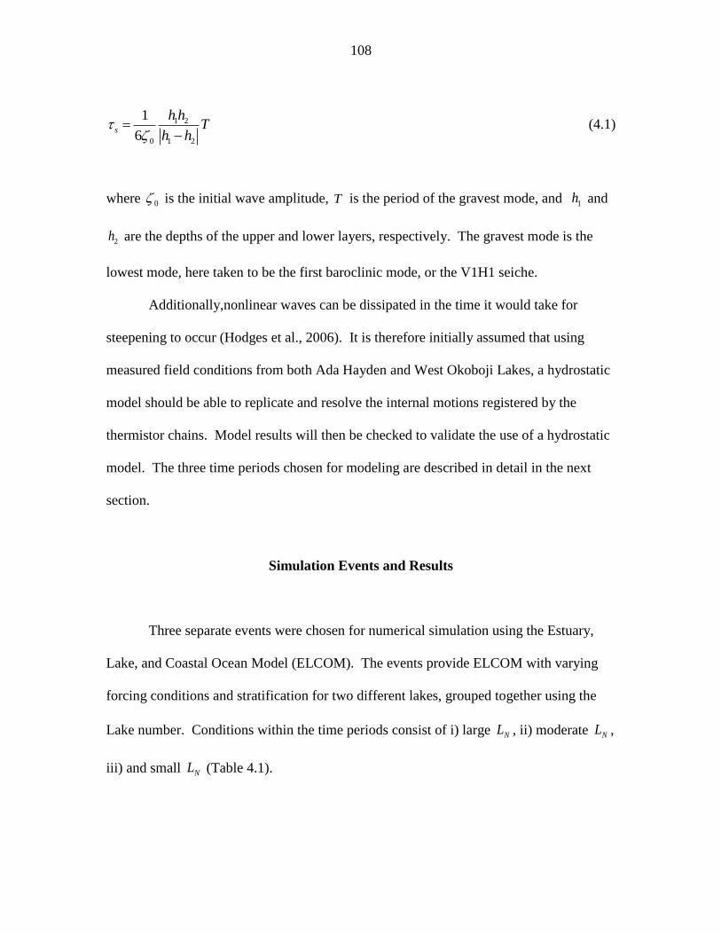
108
1 2
0 1 2
1
6s
h hT
h h
(4.1)
where 0 is the initial wave amplitude, T is the period of the gravest mode, and 1h and
2h are the depths of the upper and lower layers, respectively. The gravest mode is the
lowest mode, here taken to be the first baroclinic mode, or the V1H1 seiche.
Additionally,nonlinear waves can be dissipated in the time it would take for
steepening to occur (Hodges et al., 2006). It is therefore initially assumed that using
measured field conditions from both Ada Hayden and West Okoboji Lakes, a hydrostatic
model should be able to replicate and resolve the internal motions registered by the
thermistor chains. Model results will then be checked to validate the use of a hydrostatic
model. The three time periods chosen for modeling are described in detail in the next
section.
Simulation Events and Results
Three separate events were chosen for numerical simulation using the Estuary,
Lake, and Coastal Ocean Model (ELCOM). The events provide ELCOM with varying
forcing conditions and stratification for two different lakes, grouped together using the
Lake number. Conditions within the time periods consist of i) large NL , ii) moderate NL ,
iii) and small NL (Table 4.1).

109
Table 4.1. Summary of simulation events. is a measure of the relative top layer
thickness when representing the stratification using a two-layer model. Stratification and
forcing conditions for simulations 1-3 are combined using (range of values and
averages are given). AHL = Ada Hayden Lake, WOL = West Okoboji Lake.
Simulation Time Period Lake h1/H LN Range (Avg)
1 7-12 Aug. 2007 AHL 0.35 3-553 (115)
2 30 July-4 Aug. 2008 AHL 0.35 6-495 (89)
3 6-18 July 2009 WOL 0.32 0.01-275 (31)
Simulation 1: High Lake Number
The first event to be simulated consists of 7-12 August 2007 at Ada Hayden Lake.
This period experienced relatively calm wind and was sufficiently stratified to limit
internal motions. The initial stratification and mode shape is shown in Figure 4.9. Figure
4.9 shows the thermocline depth to be approximately 6 m when representing the lake as a
two-layer system. When considering a three-layer temperature structure, a metalimnion
of finite thickness exists, with the top and bottom at depths of approximately 4 and 9 m,
respectively. The normal mode equation (2.11) given by Münnich et al. (1992) yields a
phase speed nc for a V1H1 internal wave of approximately 0.3 m/s and a wave period of
1.3 hours. Once the phase speed is known, the horizontal grid size and time step can be
related using the expression for the CFL condition (3.1). A total of 56 simulations was
run for this event, with different grid sizes in the horizontal ( x ), vertical ( z ), and
model time steps ( t ) which correspond with x (Table 4.2).
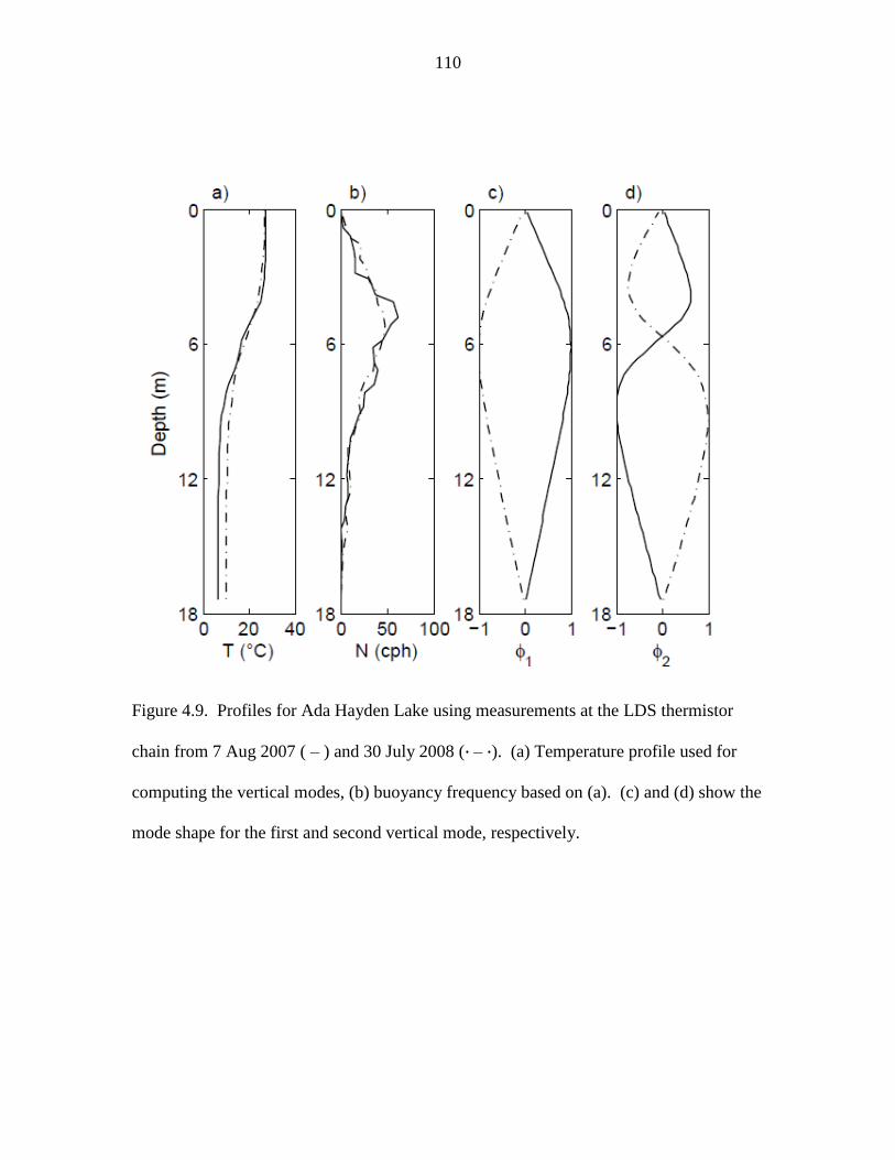
110
Figure 4.9. Profiles for Ada Hayden Lake using measurements at the LDS thermistor
chain from 7 Aug 2007 ( – ) and 30 July 2008 ( – ). (a) Temperature profile used for
computing the vertical modes, (b) buoyancy frequency based on (a). (c) and (d) show the
mode shape for the first and second vertical mode, respectively.
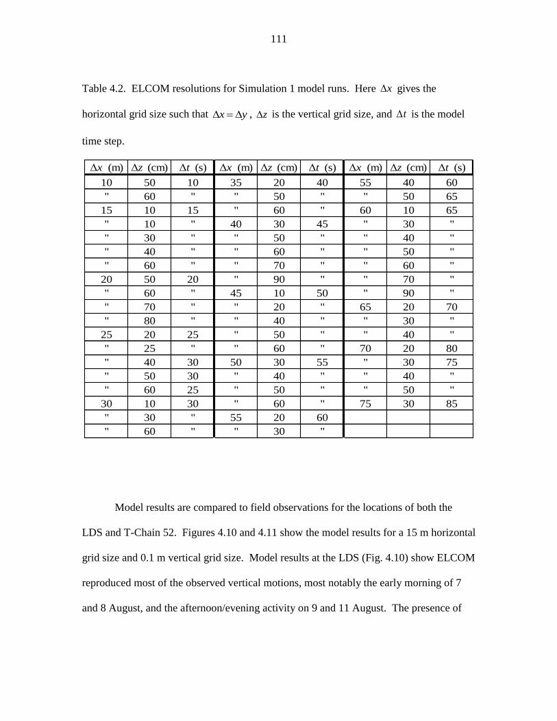
111
Table 4.2. ELCOM resolutions for Simulation 1 model runs. Here x gives the
horizontal grid size such that x y , z is the vertical grid size, and t is the model
time step.
Δx (m) Δz (cm) Δt (s) Δx (m) Δz (cm) Δt (s) Δx (m) Δz (cm) Δt (s)
10 50 10 35 20 40 55 40 60
" 60 " " 50 " " 50 65
15 10 15 " 60 " 60 10 65
" 10 " 40 30 45 " 30 "
" 30 " " 50 " " 40 "
" 40 " " 60 " " 50 "
" 60 " " 70 " " 60 "
20 50 20 " 90 " " 70 "
" 60 " 45 10 50 " 90 "
" 70 " " 20 " 65 20 70
" 80 " " 40 " " 30 "
25 20 25 " 50 " " 40 "
" 25 " " 60 " 70 20 80
" 40 30 50 30 55 " 30 75
" 50 30 " 40 " " 40 "
" 60 25 " 50 " " 50 "
30 10 30 " 60 " 75 30 85
" 30 " 55 20 60
" 60 " " 30 "
Model results are compared to field observations for the locations of both the
LDS and T-Chain 52. Figures 4.10 and 4.11 show the model results for a 15 m horizontal
grid size and 0.1 m vertical grid size. Model results at the LDS (Fig. 4.10) show ELCOM
reproduced most of the observed vertical motions, most notably the early morning of 7
and 8 August, and the afternoon/evening activity on 9 and 11 August. The presence of

112
Figure 4.10. Time series temperature profile plot for Simulation 1, measured by the LDS
for a) field data and b) ELCOM output at 15 m horizontal grid cell size and 0.1 m vertical
grid cell size.

113
Figure 4.11. Time series temperature profile plot for Simulation 1, measured by T-Chain
52 for a) field data and b) ELCOM output at 15 m horizontal grid cell size and 0.1 m
vertical grid cell size.
114
the 28 °C isotherm is not reproduced in ELCOM, most likely because of computational
errors in the non-penetrative long-wave radiation that heats the surface-mixed layer
(Hodges et al., 2000). Long-wave radiation, which is emitted from clouds and
atmospheric water vapor, is estimated in ELCOM using cloud cover, air temperature, and
humidity. Because cloud cover was not measured, ELCOM estimated long-wave
radiation for zero cloud cover. While this would underpredict some heating in the
surface mixed layer, the depth of the base of the mixed layer appeared to slightly deepen
throughout the simulation. The comparison between field observations and model output
at the location of T-Chain 52 (Fig. 4.11) shows similar results in the reproduction of
internal motions. Vertical motions tended to be more pronounced at T-Chain 52. Most
of the motion is located between the 4-9 m depth previously identified within the
metalimnion, as would be expected by inspecting the buoyancy profile.
The same event was modeled at a coarser vertical resolution with a 0.6 m vertical
grid cell size; but with the same 15 m uniform horizontal grid and the same 15 s model
time step. Results from the LDS (Fig. 4.12) and T-Chain 52 (Fig. 4.13) show lower
frequency vertical motion and a thickening of the metalimnion by the spreading of the
temperature contours. At the end of the simulations, the metalimnion thickness was 4.7
and 5.4 m for z = 0.1 and 0.6 m, respectively. ELCOM‘s ability to resolve higher
frequency motions is limited by the cell size (Hodges et al., 2000). This metalimnion
thickening is characteristic of numerical diffusion, which leads to the erosion of the
thermocline and isopycnal spreading. Figure 4.13b shows the 26°C isotherm surfacing
midday on 9 August from the model output, but no such movement is seen in the field
data. This isotherm surfacing could be caused by error in the surface thermodynamic
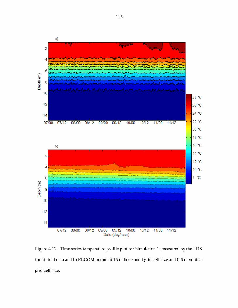
115
Figure 4.12. Time series temperature profile plot for Simulation 1, measured by the LDS
for a) field data and b) ELCOM output at 15 m horizontal grid cell size and 0.6 m vertical
grid cell size.
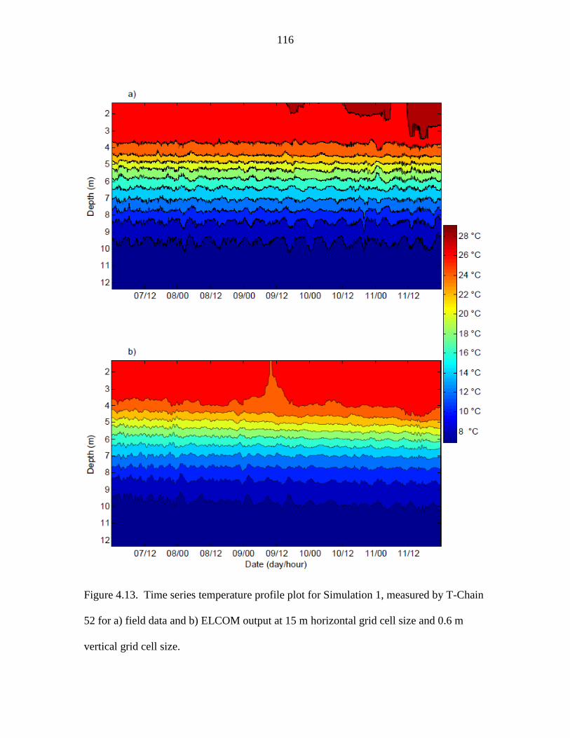
116
Figure 4.13. Time series temperature profile plot for Simulation 1, measured by T-Chain
52 for a) field data and b) ELCOM output at 15 m horizontal grid cell size and 0.6 m
vertical grid cell size.

117
model. Similar results, in terms ELCOM predicting the surfacing of isotherms not
observed in the field, can be seen in the literature (e.g., Fig. 12 in Hodges et al., 2000 and
Fig. 11 in Yeates et al., 2008), although no discussion concerning the discrepancy was
provided.
Hodges et al. (2006) gave empirical relationships for numerical diffusivity (2.61)
and numerical viscosity (2.63). These relationships show both numerical error terms
scaled inversely to the gradient Richardson number 1/3
gRi . After Yeates et al. (2008), the
Lake number NL can be substituted for gRi by using the relationship 2
g NRi L given by
Imberger (2004). Therefore, 2/3
NL can be used to estimate numerical diffusion and
numerical viscosity during a model run.
Figure 4.14a shows values for 2/3
NL computed from measured wind speed. As
numerical diffusion and viscosity have been shown to scale with 2/3
NL , magnitudes of
PE and KE are not of as much interest as the behavior between field and model results.
PE is used as the total potential energy in the water column is much larger than
comparatively small changes caused by internal waves and diurnal heating. A
normalized time series of PE is shown in Figure 4.14b. To assess the total amount of
vertical fluid movement throughout a simulation period, KE is used (Fig. 4.14c). A
strong wind event can be seen shortly after the start of the simulation on 7 August. This
increase in 2/3
NL appears to not negatively affect the model‘s performance initially in
terms of potential energy. However, the model slightly overpredicted the internal
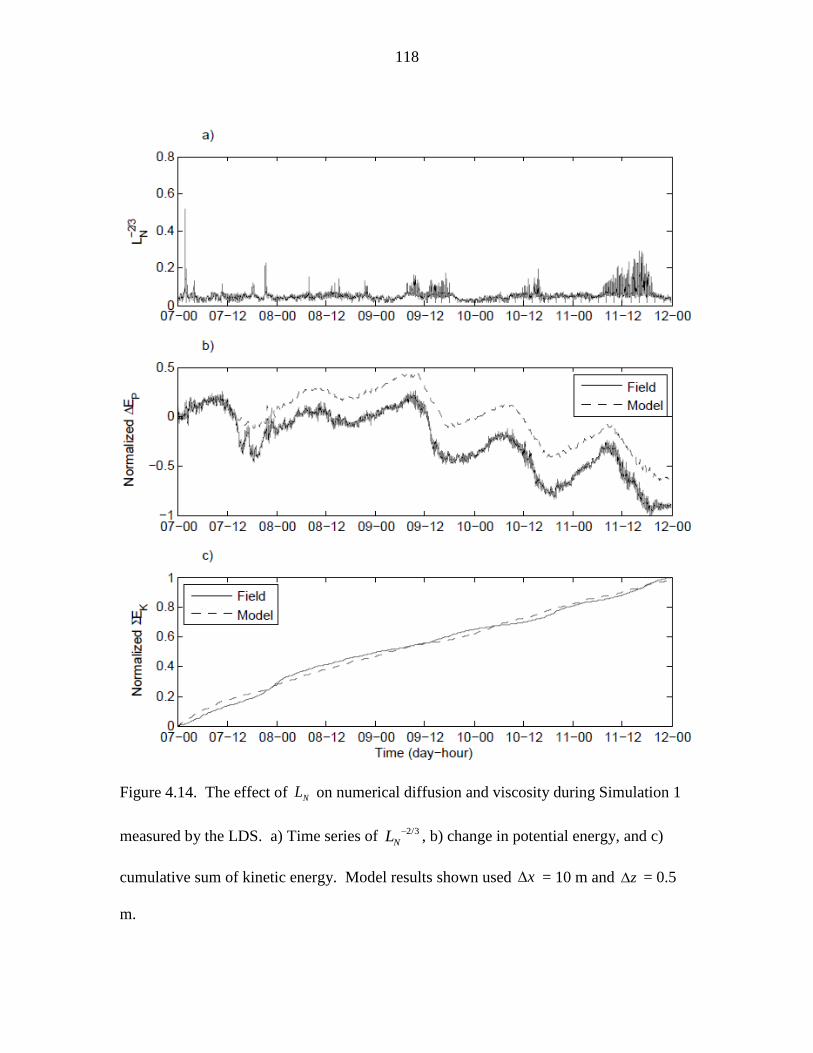
118
Figure 4.14. The effect of NL on numerical diffusion and viscosity during Simulation 1
measured by the LDS. a) Time series of 2/3
NL , b) change in potential energy, and c)
cumulative sum of kinetic energy. Model results shown used x = 10 m and z = 0.5
m.

119
motions as the model yielded higher kinetic energy values (Fig. 4.14c). A second wind
even in the evening of 7 August caused a slight increase in KE and fluctuations in PE
in the field data. The model failed to register the increase in KE , evidenced by the field
kinetic energy sum overtaking the model results (Fig. 4.14c).
Figure 4.15. Normalized time-integrated potential energy from Simulation 1, measured
by the LDS. Horizontal and vertical grid cell size is given by x and z , respectively.
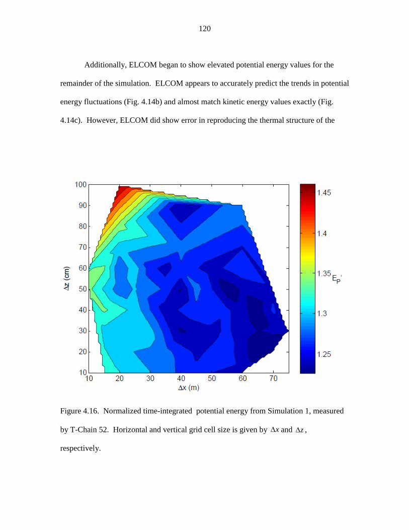
120
Additionally, ELCOM began to show elevated potential energy values for the
remainder of the simulation. ELCOM appears to accurately predict the trends in potential
energy fluctuations (Fig. 4.14b) and almost match kinetic energy values exactly (Fig.
4.14c). However, ELCOM did show error in reproducing the thermal structure of the
Figure 4.16. Normalized time-integrated potential energy from Simulation 1, measured
by T-Chain 52. Horizontal and vertical grid cell size is given by x and z ,
respectively.
121
lake, indicated by the elevated potential energy values. High potential energy values in
the model output could be caused by elevated mixing or numerical diffusion.
The normalized potential energy PE (3.20) results are shown for the values
measured by the LDS (Fig. 4.15) and T-Chain 52 (Fig. 4.16). PE > 1 indicates the
model producing a higher center of mass within the water column, while lower values
indicate a lower center of mass. A higher center of mass could be the result of either
elevated mixing in the model or numerical diffusion. Figure 4.15 shows PE values
greater than one throughout all simulations, ranging from approximately 1.3 to 1.55. The
best model results for the location of the LDS occur for lower horizontal grid sizes
(between 10 and 40 m), and vertical grid cell sizes varying between 0.3 and 0.6 m.
Interestingly, there appears to be a realm between x = 20-30 m and z = 0.2-0.4 m
where there is an increase in normalized potential energy. High PE values occur for
high vertical grid sizes of 0.8 m or higher. The results from T-Chain 52 (Fig. 4.16) are
quite similar compared to the LDS. In general, the lower the vertical grid size, the better
the model performance. However, lower values for the horizontal grid resulted in an
increase in potential energy. Therefore, best model results in terms of maintaining the
thermal structure appear to be x = 40 m and z = 0.3 m based on the results in Figs.
4.15 and 4.16.
The normalized time-integrated kinetic energy results KE (3.22) are shown in
Figures 4.17 and 4.18 for profiles at the LDS and T-Chain 52, respectively. Model
results at the LDS location show best agreement with field observations for small
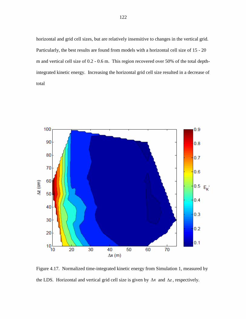
122
horizontal and grid cell sizes, but are relatively insensitive to changes in the vertical grid.
Particularly, the best results are found from models with a horizontal cell size of 15 - 20
m and vertical cell size of 0.2 - 0.6 m. This region recovered over 50% of the total depth-
integrated kinetic energy. Increasing the horizontal grid cell size resulted in a decrease of
total
Figure 4.17. Normalized time-integrated kinetic energy from Simulation 1, measured by
the LDS. Horizontal and vertical grid cell size is given by x and z , respectively.

123
kinetic energy reproduced in the model, with x values greater than 40 m yielding
values less than 10% measured in the field. Figure 4.18 gives similar results for model
performance as measured at the location of T-Chain 52; low horizontal grid sizes appear
to reproduce similar amplitude internal motions. However, unlike conditions at the LDS,
Fig 4.18 shows a concentrated area of higher kinetic energy values for x = 60 - 70 m
and z = 0.1 - 0.3 m.
Figure 4.18. Normalized time-integrated kinetic energy from Simulation 1, measured by
T-Chain 52. Horizontal and vertical grid cell size is given by x and z , respectively.

124
Figure 4.19. Displacement power spectra calculated from field data at Ada Hayden Lake
during Simulation 1 for a) 25°C, b) 17°C, and c) 12°C isotherms. Power spectra shown
for isotherm displacements measured from the LDS and T-Chain 52. The frequencies for
the V1 and V2 mode internal wave are shown as 1f and 2f , respectively.
To determine if there is a dominant internal wave frequency, a displacement
power spectra was calculated for the 25, 17, and 12°C isotherms (Fig. 4.19). The
isotherms chosen were to represent the top, middle, and bottom of the metalimnion (see

125
Fig. 4.9 for the temperature structure of the lake). The results from the spectral analysis
show no dominant frequencies at either the V1 or V2 mode seiche, simply a steady
decline in spectral density with increasing frequency. To compare model results to field
Figure 4.20. Spectral density of the displacement of the 17°C isotherm during Simulation
1. Isotherm displacement measured by the LDS and calculated using model output with
a) x = 15 m, z = 0.3 m, and b) x = 30 m, z = 0.3 m. The vertical offset for each
spectra is 103, beginning with a).
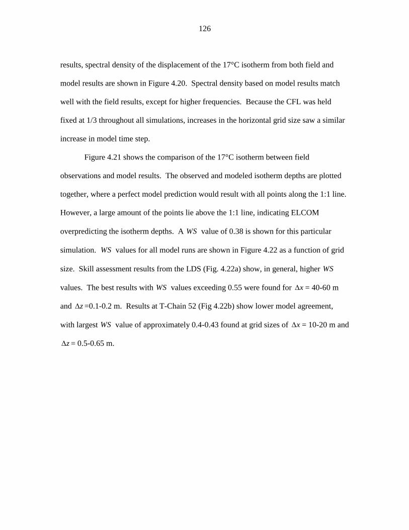
126
results, spectral density of the displacement of the 17°C isotherm from both field and
model results are shown in Figure 4.20. Spectral density based on model results match
well with the field results, except for higher frequencies. Because the CFL was held
fixed at 1/3 throughout all simulations, increases in the horizontal grid size saw a similar
increase in model time step.
Figure 4.21 shows the comparison of the 17°C isotherm between field
observations and model results. The observed and modeled isotherm depths are plotted
together, where a perfect model prediction would result with all points along the 1:1 line.
However, a large amount of the points lie above the 1:1 line, indicating ELCOM
overpredicting the isotherm depths. A WS value of 0.38 is shown for this particular
simulation. WS values for all model runs are shown in Figure 4.22 as a function of grid
size. Skill assessment results from the LDS (Fig. 4.22a) show, in general, higher WS
values. The best results with WS values exceeding 0.55 were found for x = 40-60 m
and z =0.1-0.2 m. Results at T-Chain 52 (Fig 4.22b) show lower model agreement,
with largest WS value of approximately 0.4-0.43 found at grid sizes of x = 10-20 m and
z = 0.5-0.65 m.
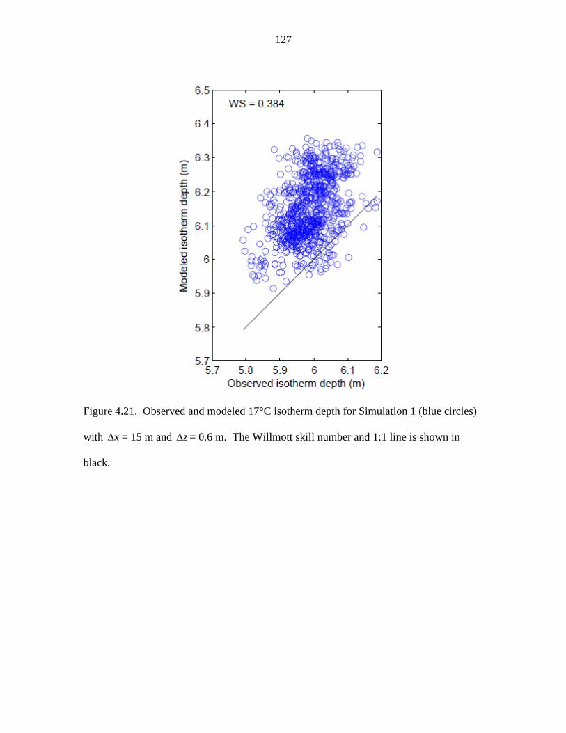
127
Figure 4.21. Observed and modeled 17°C isotherm depth for Simulation 1 (blue circles)
with x = 15 m and z = 0.6 m. The Willmott skill number and 1:1 line is shown in
black.
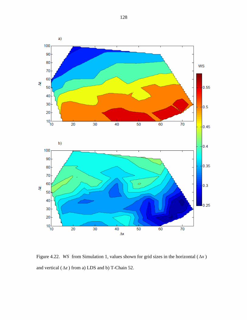
128
Figure 4.22. WS from Simulation 1, values shown for grid sizes in the horizontal ( x )
and vertical ( z ) from a) LDS and b) T-Chain 52.
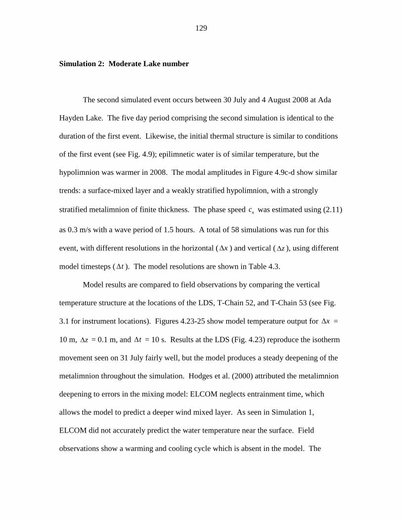
129
Simulation 2: Moderate Lake number
The second simulated event occurs between 30 July and 4 August 2008 at Ada
Hayden Lake. The five day period comprising the second simulation is identical to the
duration of the first event. Likewise, the initial thermal structure is similar to conditions
of the first event (see Fig. 4.9); epilimnetic water is of similar temperature, but the
hypolimnion was warmer in 2008. The modal amplitudes in Figure 4.9c-d show similar
trends: a surface-mixed layer and a weakly stratified hypolimnion, with a strongly
stratified metalimnion of finite thickness. The phase speed nc was estimated using (2.11)
as 0.3 m/s with a wave period of 1.5 hours. A total of 58 simulations was run for this
event, with different resolutions in the horizontal ( x ) and vertical ( z ), using different
model timesteps ( t ). The model resolutions are shown in Table 4.3.
Model results are compared to field observations by comparing the vertical
temperature structure at the locations of the LDS, T-Chain 52, and T-Chain 53 (see Fig.
3.1 for instrument locations). Figures 4.23-25 show model temperature output for x =
10 m, z = 0.1 m, and t = 10 s. Results at the LDS (Fig. 4.23) reproduce the isotherm
movement seen on 31 July fairly well, but the model produces a steady deepening of the
metalimnion throughout the simulation. Hodges et al. (2000) attributed the metalimnion
deepening to errors in the mixing model: ELCOM neglects entrainment time, which
allows the model to predict a deeper wind mixed layer. As seen in Simulation 1,
ELCOM did not accurately predict the water temperature near the surface. Field
observations show a warming and cooling cycle which is absent in the model. The

130
Table 4.3. ELCOM resolutions for model runs of Simulation 2. Here x gives the
horizontal grid size such that x y , z is the vertical grid size, and t is the model
time step.
Δx (m) Δz (cm) Δt (s) Δx (m) Δz (cm) Δt (s) Δx (m) Δz (cm) Δt (s)
10 10 10 25 85 30 55 15 65
" 50 " " 95 " " 25 "
" 75 " 35 15 40 " 35 "
" 100 " " 25 " " 45 "
15 15 15 " 35 " " 55 "
" 25 20 " 45 " " 65 "
" 35 " " 55 " " 75 "
" 45 " " 65 " " 85 "
" 55 " " 75 " " 95 "
" 65 " " 85 " 65 15 80
" 75 " " 95 " " 25 "
" 85 " 45 15 55 " 35 "
" 95 " " 25 " " 45 "
25 15 30 " 35 " " 55 "
" 25 " " 45 " " 65 "
" 35 " " 55 " " 75 "
" 45 " " 65 " " 85 "
" 55 " " 75 " " 95 "
" 65 " " 85 "
" 75 " " 95 "
amplitude of the internal wave was underestimated by ELCOM, which can be attributed
to numerical dissipation. The large amplitude motion on 31 July predicted by ELCOM
was approximately 78% of the results measured in the field. Hodges et al. (2000) cited
numerical damping of the Kelvin wave during simulations of Lake Kinneret, while
Gomez-Giraldo et al. (2006) observed an approximate 20% reduction in internal wave
amplitude caused by numerical dissipation due to the no-normal-flow boundary condition
131
applied to a coarse grid model. Therefore, the observed damping is similar to values
given in the literature.
The model results at the thermistor chain locations are similar to those depicted at
the LDS. Figure 4.24 shows the comparison between field observations and model
output at the location of T-Chain 52. As was seen at the LDS, the internal wave
oscillations on 31 July are reproduced by ELCOM, but the overall magnitude is
underestimated. Field data shows the 22 and 24°C isotherms rising by approximately 1
m, that motion is damped in the model. Figure 4.25 shows that T-Chain 53 experienced
more internal wave activity, both in the duration of activity on 31 July and on 3 August.
The surface temperature fluxes are not correctly reproduced: field observations show
surface heating from 31 July - 3 August that was not present in the model. ELCOM
predicted upward movement of the 24°C isotherm beginning 2 August at both thermistor
chain locations. This surfacing was not observed in the field, perhaps indicating errors in
the mixing model, the wind momentum model, or in the numerical scheme.
Figure 4.26a shows values for 2/3
NL computed from measured wind speed. As
numerical diffusion and viscosity have been shown to scale with 2/3
NL , magnitudes of
PE and KE are not of as much interest as the behavior between field and model results.
As previously discussed, PE is used as the changes due to internal wave perturbations
are small, and is shown in Figure 4.26b. Similarly, KE values tend to be small as
velocities in the column tend to be slow. To gain a feeling of the total amount of vertical
fluid movement throughout a time period, KE is shown in Figure 4.26c. A low NL
event occurred on 31 July, and while field observations show a marked increase in
132
Figure 4.23. Time series temperature profile plot for Simulation 2, measured by the LDS
for a) field data and b) ELCOM output at 10 m horizontal grid cell size and 0.1 m vertical
grid cell size.

133
Figure 4.24. Time series temperature profile plot for Simulation 2, measured by T-Chain
52 for a) field data and b) ELCOM output at 10 m horizontal grid cell size and 0.1 m
vertical grid cell size.

134
Figure 4.25. Time series temperature profile plot for Simulation 2, measured by T-Chain
53 for a) field data and b) ELCOM output at 10 m horizontal grid cell size and 0.1 m
vertical grid cell size.
135
movement, ELCOM registered very little change. Again, strong winds act to set up
internal wave action periodically throughout 1-4 August, causing oscillations measured
by the LDS, but the model shows little increase in KE .
Additional model runs for Simulation 2 support the results previously discussed:
numerical viscosity appears to damp internal wave amplitudes and drives the isotherms in
the metalimnion down, lowering the center of gravity. This results in a decrease in both
PE and KE . Results for PE are shown in Figures 4.27-29 for the LDS, T-Chain 52,
and T-Chain 53, respectively. Figure 4.27 shows that for the simulations at small grid
sizes, model results show a deepening of isotherms in the metalimnion. At higher values
of z , this deepening effect is reduced, and the model more closely matches field
observations in terms of the retention of a vertical thermal structure. Figure 4.28 shows
similar results for T-Chain 52; small grid sizes result in lower PE values, and larger
values for z give results much closer to one. Figure 4.29 shows better model
performance for T-Chain 53 than compared to the results in Figure 4.28. Smaller grid
sizes do show values less than one; however, there is a region for z = 0.3 - 0.6 m for
x = 10 m which gives PE values close to one.
Results for KE are shown in Figures 4.30-32 for the LDS, T-Chain 52, and T-
Chain 53, respectively. All three plots show similar results: kinetic energy is most
accurately reproduced for small x and z and least precisely for higher z values.
However, small horizontal grid cells do provide acceptable results for z = 0.1 - 0.6 m,

136
Figure 4.26. The effect of NL on numerical diffusion and viscosity during Simulation 2
measured by the LDS. a) Time series of 2/3
NL , b) change in potential energy, and c)
cumulative sum of kinetic energy. Model results shown used x = 10 m and z = 0.5
m.

137
Figure 4.27. Normalized time-integrated potential energy for Simulation 2 measured at
the LDS. Horizontal and vertical grid cell size is given by x and z , respectively.
indicating that KE is more sensitive to changes in x than z . Considering the best
case model prediction, ELCOM underestimates by approximately 30%. This
underestimation has implications for transport of scalars in the water body (i.e., dissolved
oxygen, phytoplankton, nutrients, etc.) Therefore, considering both the reproduction of
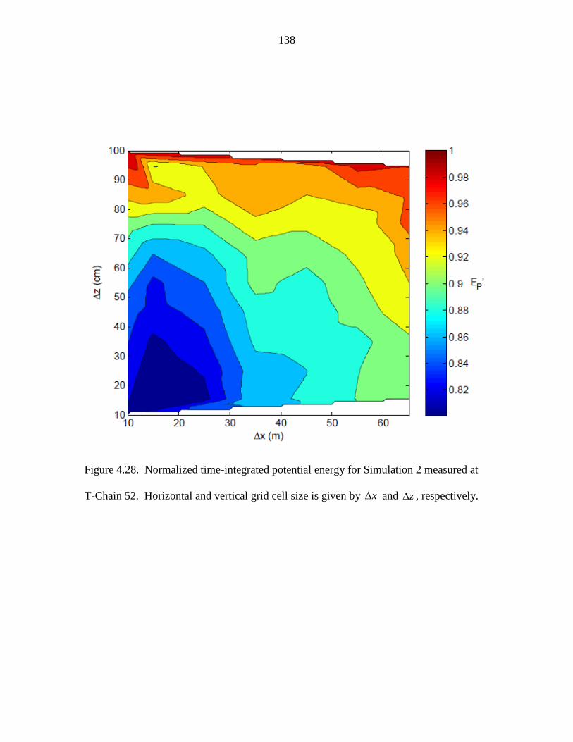
138
Figure 4.28. Normalized time-integrated potential energy for Simulation 2 measured at
T-Chain 52. Horizontal and vertical grid cell size is given by x and z , respectively.
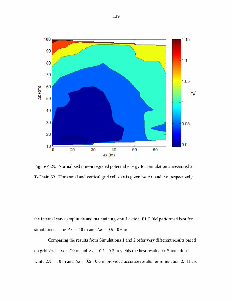
139
Figure 4.29. Normalized time-integrated potential energy for Simulation 2 measured at
T-Chain 53. Horizontal and vertical grid cell size is given by x and z , respectively.
the internal wave amplitude and maintaining stratification, ELCOM performed best for
simulations using x = 10 m and z = 0.5 - 0.6 m.
Comparing the results from Simulations 1 and 2 offer very different results based
on grid size: x = 20 m and z = 0.1 - 0.2 m yields the best results for Simulation 1
while x = 10 m and z = 0.5 - 0.6 m provided accurate results for Simulation 2. These
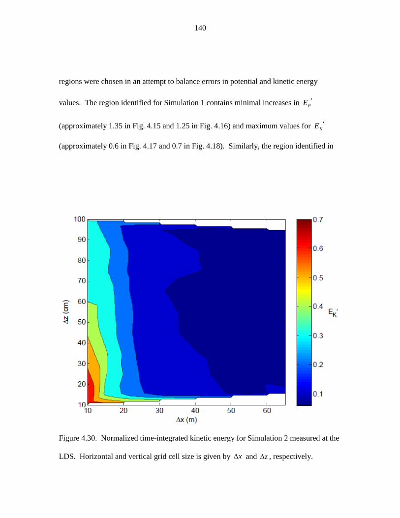
140
regions were chosen in an attempt to balance errors in potential and kinetic energy
values. The region identified for Simulation 1 contains minimal increases in PE
(approximately 1.35 in Fig. 4.15 and 1.25 in Fig. 4.16) and maximum values for KE
(approximately 0.6 in Fig. 4.17 and 0.7 in Fig. 4.18). Similarly, the region identified in
Figure 4.30. Normalized time-integrated kinetic energy for Simulation 2 measured at the
LDS. Horizontal and vertical grid cell size is given by x and z , respectively.
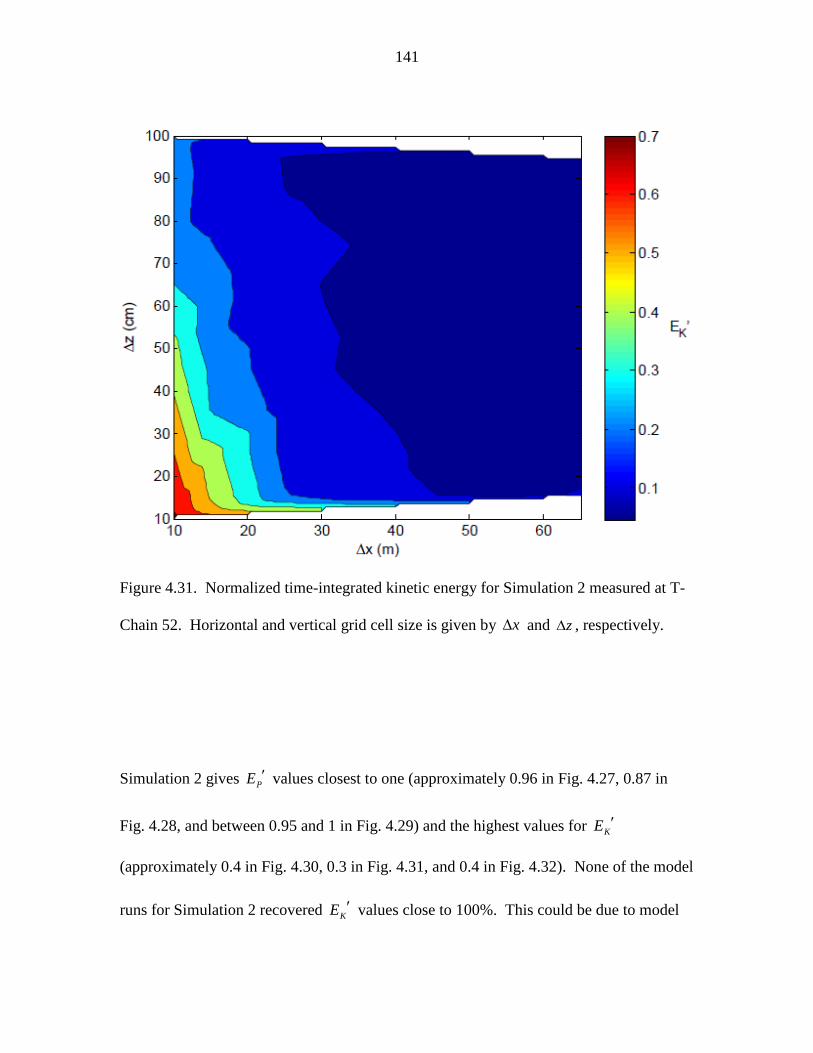
141
Figure 4.31. Normalized time-integrated kinetic energy for Simulation 2 measured at T-
Chain 52. Horizontal and vertical grid cell size is given by x and z , respectively.
Simulation 2 gives PE values closest to one (approximately 0.96 in Fig. 4.27, 0.87 in
Fig. 4.28, and between 0.95 and 1 in Fig. 4.29) and the highest values for KE
(approximately 0.4 in Fig. 4.30, 0.3 in Fig. 4.31, and 0.4 in Fig. 4.32). None of the model
runs for Simulation 2 recovered KE values close to 100%. This could be due to model

142
errors in calculating momentum input, in the vertical mixing model, or damping due to
numerical viscosity in the advection scheme.
To assess ELCOM‘s ability to reproduce internal vertical motions, power spectra
of the displacement of the 17°C isotherm were calculated from both field and model
results (Fig. 4.33). The model power spectra match field results at low frequencies,
particularly in reproducing the troughs in the spectral density at 0.6 and 1.3 cpd.
Figure 4.32. Normalized time-integrated kinetic energy for Simulation 2, measured by T-
Chain 53. Horizontal and vertical grid cell size is given by x and z , respectively.

143
Figure 4.33. Spectral density of the displacement of the 17°C isotherm during Simulation
2. Isotherm displacement measured by the LDS and calculated using model output with
a) x = 10 m, z = 0.1 m, and b) x = 10 m, z = 0.5 m. The vertical offset for each
spectra is 103, beginning with a).
Figure 4.34 shows the comparison of the 17°C isotherm between field
observations and model results. A large amount of the points lie above the 1:1 line,
indicating ELCOM overpredicting the isotherm depths, as in Simulation 1. WS values
for all model runs are shown in Figure 4.35 as a function of grid size. Skill assessment

144
Figure 4.34. Observed and modeled 17°C isotherm depth for Simulation 2 (blue circles)
with x = 10 m and z = 0.5 m. The Willmott skill number and 1:1 line is shown in
black.
results from the LDS (Fig. 4.35a) show highest WS values of approximately 0.24 for
small vertical grid sizes of z =0.1-0.2 m and a wider range in the horizontal grid size
with x =10-30 m. Results from T-Chain 52 (Fig 4.35b) show slightly different results
in that the region of best skill is for 0.2 0.4z m and x =15-25 m yielding WS =
0.21-0.22. This region corresponds to a coarser vertical grid than identified in Figure

145
Figure 4.35. WS from Simulation 2, values shown for grid sizes in the horizontal ( x )
and vertical ( z ) from a) LDS, b) T-Chain 52, and c)
T-Chain 53.

146
4.35a. The results shown in Figure 4.35c for T-Chain 53 are similar to the results from
T-Chain 52, except higher WS values of 0.26-0.28 for 0.2 0.4z m and x =15-35
m.
Simulation 3: Low Lake number
The third simulation period consists of 6-18 July 2009 at West Okoboji Lake.
This period experienced stronger winds than Ada Hayden Lake with less stratification,
resulting in greater internal wave amplitudes. The initial stratification and mode shape is
shown in Figure 4.36. The LDS was deployed in 25 m deep water; however, the deepest
section of West Okoboji Lake approaches 43 m. To fill in the missing temperature data
at depths greater than 25 m, data were obtained from Iowa State University Limnology
Laboratory, which measured temperature to a depth of 40 m. The phase speed nc
corresponding to the temperature profile in Figure 4.36 was calculated as 0.28 m/s and
the wave period is approximately 13 hours. A total of 56 simulations was run for this
event, with different grid sizes in the horizontal ( x ), vertical ( z ), and model time
steps ( t ) (Table 4.4).
Model results are compared to field observations for Simulation 3 for the
locations of both the LDS and T-Chain 52. ELCOM reproduced internal motions but did
not accurately match temperatures in both the surface layer and hypolimnion (Fig. 4.37).
Field measurements showed surface heating from 11-14 July; while ELCOM did give
some periodic heating, the result was not to the same extent as observed in the field.
Additionally, the 14°C isotherm was measured to oscillate at a depth of approximately 20
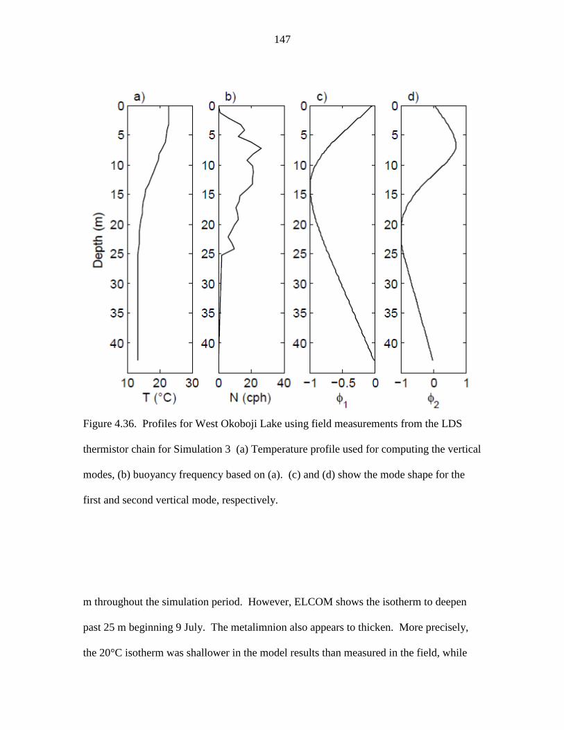
147
Figure 4.36. Profiles for West Okoboji Lake using field measurements from the LDS
thermistor chain for Simulation 3 (a) Temperature profile used for computing the vertical
modes, (b) buoyancy frequency based on (a). (c) and (d) show the mode shape for the
first and second vertical mode, respectively.
m throughout the simulation period. However, ELCOM shows the isotherm to deepen
past 25 m beginning 9 July. The metalimnion also appears to thicken. More precisely,
the 20°C isotherm was shallower in the model results than measured in the field, while

148
Table 4.4 ELCOM resolutions for model runs of Simulation 3. Here x gives the
horizontal grid size such that x y , z is the vertical grid size, and t is the model
time step.
Δx (m) Δz (cm) Δt (s) Δx (m) Δz (cm) Δt (s) Δx (m) Δz (cm) Δt (s)
50 50 60 100 100 120 250 175 300
" 60 " " 110 " " 200 "
" 70 " " 120 " 300 120 350
" 80 " " 130 " 350 50 425
" 90 " " 140 " " 60 "
" 100 " " 150 " " 70 "
" 110 " " 175 " " 80 "
" 120 " " 200 " " 90 "
" 130 " 150 50 180 " 100 "
" 140 " " 60 " " 110 "
" 150 " " 70 " " 120 "
" 175 " " 80 " " 130 "
" 200 " " 90 " " 140 "
75 50 90 " 100 " " 150 "
" 60 " " 110 " " 175 "
" 70 " " 120 " " 200 "
" 80 " " 130 " 450 50 550
" 90 " " 140 " " 60 "
" 100 " " 150 " " 70 "
" 110 " " 175 " " 80 "
" 120 " " 200 " " 90 "
" 130 " 250 60 300 " 100 "
" 140 " " 70 " " 110 "
" 150 " " 80 " " 120 "
" 175 " " 90 " " 130 "
" 200 " " 100 " " 140 "
100 50 120 " 110 " " 150 "
" 60 " " 120 " " 175 "
" 70 " " 130 " " 200 "
" 80 " " 140 "
" 90 " " 150 "
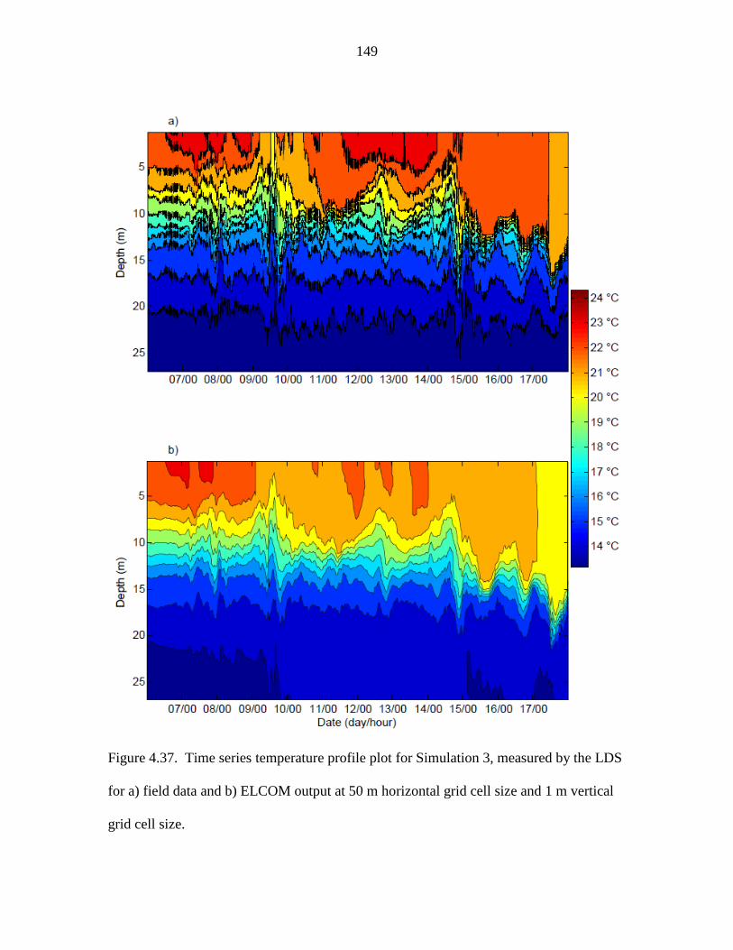
149
Figure 4.37. Time series temperature profile plot for Simulation 3, measured by the LDS
for a) field data and b) ELCOM output at 50 m horizontal grid cell size and 1 m vertical
grid cell size.

150
Figure 4.38. Time series temperature profile plot for Simulation 3, measured by T-Chain
52 for a) field data and b) ELCOM output at 50 m horizontal grid cell size and 1 m
vertical grid cell size.

151
the 15°C isotherm was deeper according to the model. The results from T-Chain 52 (Fig.
4.38) are similar to those measured by the LDS. The internal wave motions are
reproduced in terms of phase, but the amplitudes appear to be slightly damped. As was
the case at the LDS, ELCOM underestimated surface heating, resulting in the surface
layer approximately 1°C cooler than was measured in the field. The model predicts much
of the low-frequency motion but not the high-frequency oscillations, probably because
t > 15 s, the sampling time of the thermistor chains. Figure 4.39 shows how NL , PE ,
and KE vary with time.
Overall, the potential energy based on model results appears to match field
observations quite well (Fig. 4.39b). Towards the end of the simulation, a spiked
increase in NL causes an increase in the potential energy. The kinetic energy is not as
accurately modeled (Fig. 4.39c), as the model shows a consistent underestimation.
Therefore, numerical diffusion and numerical dissipation appear to affect the model
results: the model is initially damped and stratification is well modeled, but under strong
forcing conditions associated with a decrease in NL in the model shows elevated
diffusion and an increase in kinetic energy.
Values for PE measured at the LDS are shown in Figure 4.40 for simulations
using different resolutions. The results show best model performance for x in the range
of 50-100 m and z between 1-2 m. The worst results are for x = 250 m for all
vertical grid sizes. Potential energy begins to decrease again for a horizontal grid greater
than 300 m. The results from PE values calculated from T-Chain 52 are shown in Figure
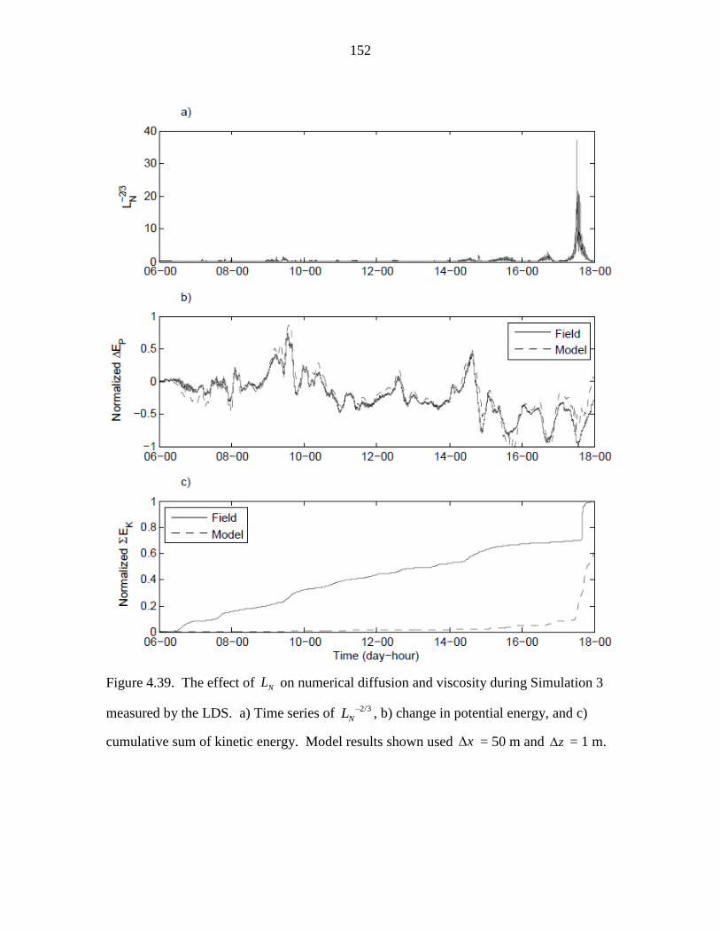
152
Figure 4.39. The effect of NL on numerical diffusion and viscosity during Simulation 3
measured by the LDS. a) Time series of 2/3
NL , b) change in potential energy, and c)
cumulative sum of kinetic energy. Model results shown used x = 50 m and z = 1 m.

153
Figure 4.40. Normalized time-integrated potential energy for Simulation 3 at the LDS.
Horizontal and vertical grid cell size is given by x and z , respectively.
4.41. Here, ELCOM performs best for high vertical grid sizes, similar to the results
calculated from the LDS. The results appear to be almost independent of the vertical
resolution for a set x with near constant values along x = 75, 200, 300, 350, and
400m. Only until the vertical grid size is in the range of 1-1.5 m does the vertical
resolution appear to become important. Examining both Figures 4.40-41, the best results
are for high horizontal resolution with a vertical grid cell size of 1-1.25 m. For results

154
from both the LDS and T-Chain 52, the model agreement is within 10-30% of field
observations.
Values for KE are shown in Figures 4.42 and 4.43 for the LDS and T-Chain 52,
respectively. Both figures have similar results in terms of the effect of horizontal grid
size: between 10-70% of the kinetic energy is recovered, with smaller x yields higher
values of KE . The difference between the two figures is the effect z has on the results.
Figure 4.41. Normalized time-integrated potential energy Simulation 3 at T-Chain 52.
Horizontal and vertical grid cell size is given by x and z , respectively.
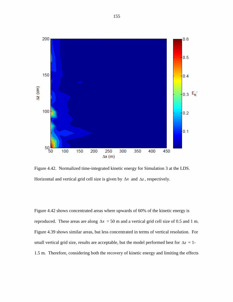
155
Figure 4.42. Normalized time-integrated kinetic energy for Simulation 3 at the LDS.
Horizontal and vertical grid cell size is given by x and z , respectively.
Figure 4.42 shows concentrated areas where upwards of 60% of the kinetic energy is
reproduced. These areas are along x = 50 m and a vertical grid cell size of 0.5 and 1 m.
Figure 4.39 shows similar areas, but less concentrated in terms of vertical resolution. For
small vertical grid size, results are acceptable, but the model performed best for z = 1-
1.5 m. Therefore, considering both the recovery of kinetic energy and limiting the effects
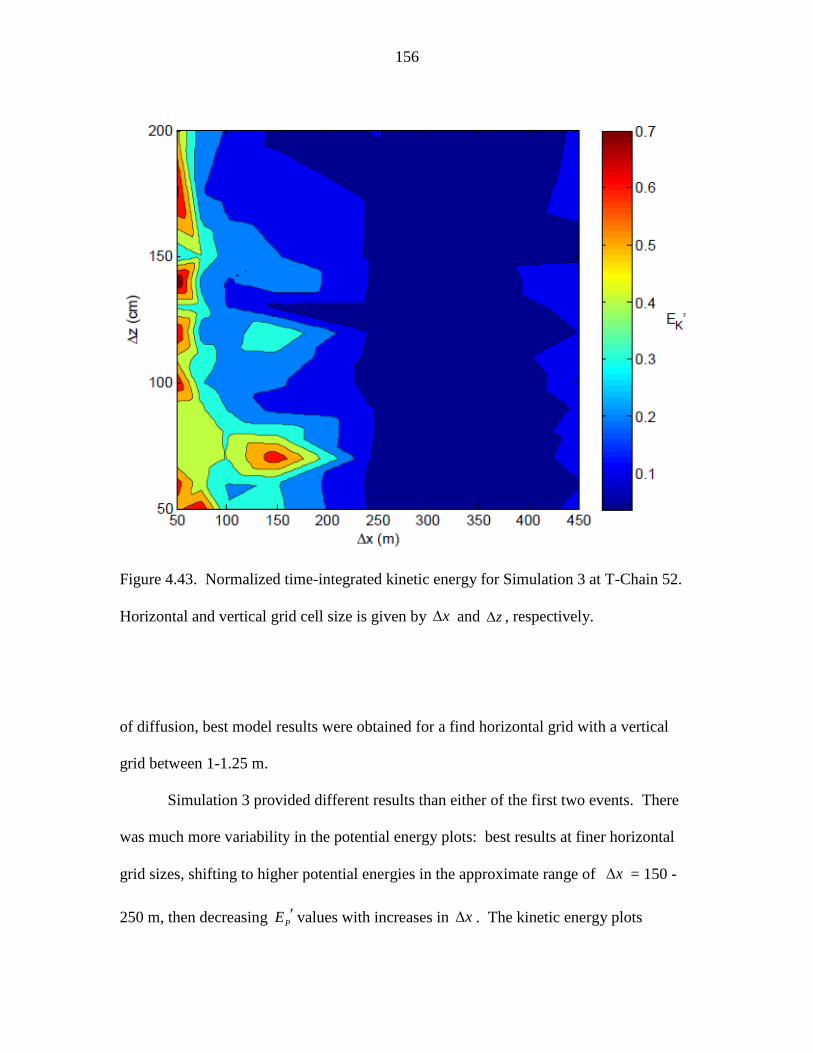
156
Figure 4.43. Normalized time-integrated kinetic energy for Simulation 3 at T-Chain 52.
Horizontal and vertical grid cell size is given by x and z , respectively.
of diffusion, best model results were obtained for a find horizontal grid with a vertical
grid between 1-1.25 m.
Simulation 3 provided different results than either of the first two events. There
was much more variability in the potential energy plots: best results at finer horizontal
grid sizes, shifting to higher potential energies in the approximate range of x = 150 -
250 m, then decreasing PE values with increases in x . The kinetic energy plots

157
behaved similarly to both previous simulations: lower horizontal grid sizes gave the best
recovery of kinetic energy. Simulations 2 and 3 had similar regions where the model
most closely agreed with field observations: the smallest horizontal grid size used ( x =
10 m for Simulation 2 and x = 50 m in Simulation 3) and vertical grid sizes slightly
Figure 4.44. Spectral density of the displacement of the 18.5°C isotherm during
Simulation 3. Isotherm displacement measured by the LDS and calculated using model
output with a) x = 50 m, z = 0.5 m, and b) x = 50 m, z = 1.5 m. The vertical
offset for each spectra is 103, beginning with a).
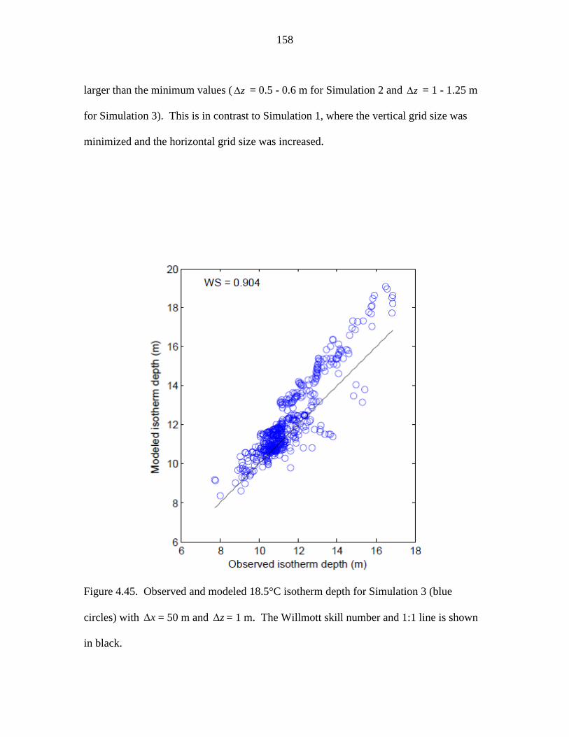
158
larger than the minimum values ( z = 0.5 - 0.6 m for Simulation 2 and z = 1 - 1.25 m
for Simulation 3). This is in contrast to Simulation 1, where the vertical grid size was
minimized and the horizontal grid size was increased.
Figure 4.45. Observed and modeled 18.5°C isotherm depth for Simulation 3 (blue
circles) with x = 50 m and z = 1 m. The Willmott skill number and 1:1 line is shown
in black.

159
Power spectra were calculated for Simulation 3 from both field data and model
output (Fig. 4.44). Spectral density based on model results match well with the field
results, especially for frequencies lower than 3 cpd. At higher frequencies, the spectral
density is limited by ELCOM‘s time steps, which varied from 60-550 s. However, given
that the frequency of the V1H1 wave is approximately 2 cpd, motions at basin-scale
frequencies were accurately modeled.
Figure 4.45 shows the comparison of the 18.5°C isotherm between field
observations and model results. Many of the points lie close to the 1:1 line or parallel
with a similar slope, indicating accurate model predictions of the isotherm depth. The
WS value of 0.9 shown in Figure 4.45 is much higher than 0.38 and 0.18 from model
runs of Simulation 1 and 2, respectively. WS values for all model runs are shown in
Figure 4.46 as a function of grid size. Skill assessment results from the LDS (Fig. 4.46a)
show highest WS values between 0.85 and exceeding 0.9 in a region given by z =0.5-1
m and x =50-400 m. Results from T-Chain 52 (Fig 4.46b) show WS =0.85 for x =100
m and z =0.5-1 m.
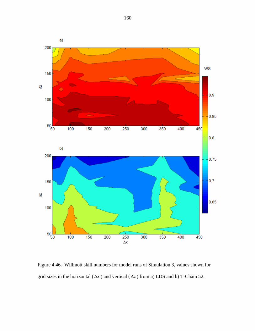
160
Figure 4.46. Willmott skill numbers for model runs of Simulation 3, values shown for
grid sizes in the horizontal ( x ) and vertical ( z ) from a) LDS and b) T-Chain 52.

161
Combining Simulation Results
The three simulation events provided different results which were quantified by
the reproduction of various forms of energy. Simulation 1 was affected by numerical
dissipation, but dominated by numerical diffusion. Results from Simulation 2 showed
excessive numerical dissipation and a decrease in potential energy due to the deepening
of isotherms in the metalimnion. Simulation 3 was adversely affected by both numerical
dissipation and numerical diffusion. To analyze the overall results from multiple
locations, scaling the grid sizes by length scales collapses the data. The results from each
simulation are combined by scaling the horizontal and vertical grid cell size by the
wavelength and total depth H , respectively (Table 4.5). The wavelength was
estimated as twice the basin length for each lake. The scaling yields the model resolution
in the horizontal / x and vertical /H x directions. These resolutions correspond to
the number of cells used to resolve the wave (or the number of points per wavelength or
depth, respectively).
Based on the combined results from Simulation 1 (Fig. 4.47), under high NL
conditions, model performance was best for a horizontal resolution ( / x ) of
approximately 75-120 and a vertical resolution ( /H z ) between 120-175 in order to
minimize increases in potential energy and maximize the vertical movement and
frequency of isotherm displacements. Errors in potential energy in this selected region
were between 30-35%, and the kinetic energy was within 10-40% of field observations.
Additionally, Willmott skill numbers for this region varied from 0.35-0.5.
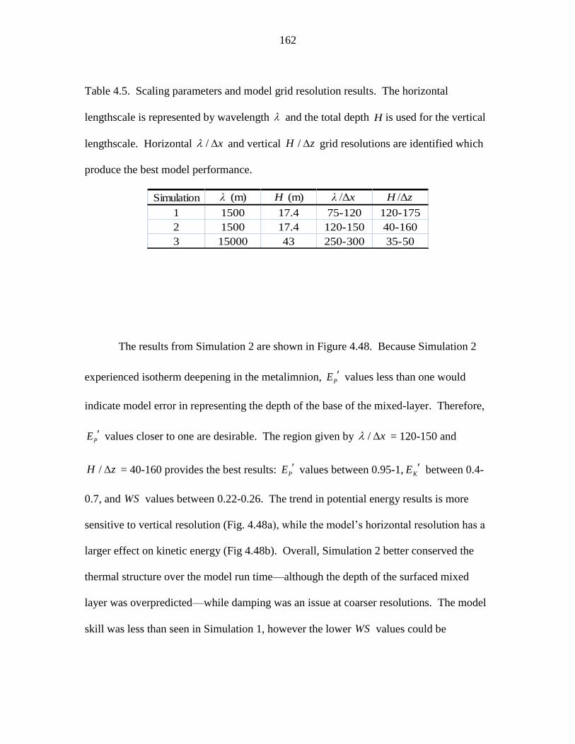
162
Table 4.5. Scaling parameters and model grid resolution results. The horizontal
lengthscale is represented by wavelength and the total depth H is used for the vertical
lengthscale. Horizontal / x and vertical /H z grid resolutions are identified which
produce the best model performance.
Simulation λ (m) H (m) λ /Δx H /Δz
1 1500 17.4 75-120 120-175
2 1500 17.4 120-150 40-160
3 15000 43 250-300 35-50
The results from Simulation 2 are shown in Figure 4.48. Because Simulation 2
experienced isotherm deepening in the metalimnion, PE values less than one would
indicate model error in representing the depth of the base of the mixed-layer. Therefore,
PE values closer to one are desirable. The region given by / x = 120-150 and
/H z = 40-160 provides the best results: PE values between 0.95-1, KE between 0.4-
0.7, and WS values between 0.22-0.26. The trend in potential energy results is more
sensitive to vertical resolution (Fig. 4.48a), while the model‘s horizontal resolution has a
larger effect on kinetic energy (Fig 4.48b). Overall, Simulation 2 better conserved the
thermal structure over the model run time—although the depth of the surfaced mixed
layer was overpredicted—while damping was an issue at coarser resolutions. The model
skill was less than seen in Simulation 1, however the lower WS values could be
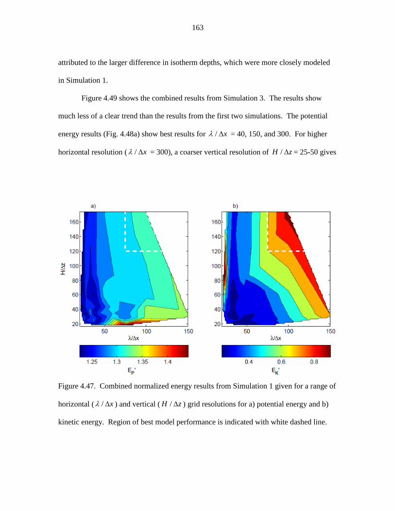
163
attributed to the larger difference in isotherm depths, which were more closely modeled
in Simulation 1.
Figure 4.49 shows the combined results from Simulation 3. The results show
much less of a clear trend than the results from the first two simulations. The potential
energy results (Fig. 4.48a) show best results for / x = 40, 150, and 300. For higher
horizontal resolution ( / x = 300), a coarser vertical resolution of /H z = 25-50 gives
Figure 4.47. Combined normalized energy results from Simulation 1 given for a range of
horizontal ( / x ) and vertical ( /H z ) grid resolutions for a) potential energy and b)
kinetic energy. Region of best model performance is indicated with white dashed line.

164
Figure 4.48. Combined normalized energy results from Simulation 2 given for a range of
horizontal ( / x ) and vertical ( /H z ) grid resolutions for a) potential energy and b)
kinetic energy. Region of best model performance is indicated with white dashed line.
the least increase in PE . The KE results show a clear trend for better results using
higher horizontal resolutions; / x = 250-300 and /H z = 30-45 and 65-85 are
regions in which kinetic energy is maximized. Overall, the results from Figure 4.48 show
best model performance for a higher horizontal resolution of 300 and across the entire
vertical resolution. However, a smaller region with a coarser vertical resolution of 35-50
was selected with the following results: errors in potential energy are within 17-21% of
field values, kinetic energy errors are within 35-50%, and skill values between 0.8-0.9.
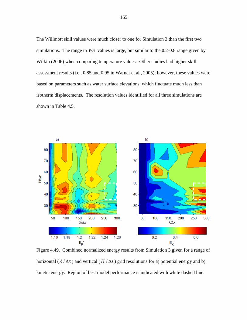
165
The Willmott skill values were much closer to one for Simulation 3 than the first two
simulations. The range in WS values is large, but similar to the 0.2-0.8 range given by
Wilkin (2006) when comparing temperature values. Other studies had higher skill
assessment results (i.e., 0.85 and 0.95 in Warner et al., 2005); however, these values were
based on parameters such as water surface elevations, which fluctuate much less than
isotherm displacements. The resolution values identified for all three simulations are
shown in Table 4.5.
Figure 4.49. Combined normalized energy results from Simulation 3 given for a range of
horizontal ( / x ) and vertical ( /H z ) grid resolutions for a) potential energy and b)
kinetic energy. Region of best model performance is indicated with white dashed line.
166
Figure 4.47-49 provide results for simulations at different NL conditions.
However, integrating analyses from multiple simulations would yield results which are
independent of the stratification and forcing conditions. Simulations 1 and 3 behaved
similarly in that both experienced increases in PE , while Simulation 3 also experienced
sufficient damping. Additionally, these two events encompassed the most extreme of the
conditions modeled: Simulation 1 modeled high NL conditions while Simulation 3
experienced large amplitude motions due to low NL . Figure 4.50 shows the results of
combining the two simulations.
To maximize model performance, a region was selected which minimized pE
and maximized KE . This region was given by the approximate resolution ranges of
/ x = 150-225 and /H z = 95-140. This region, indicated in Figure 4.50, resulted in
a 25% error in both PE and KE estimates. Additionally, this region is on the border of
the results from Simulation 1 for horizontal resolution and Simulation 3 for vertical
resolution. Therefore, it could be considered to be weighted approximately equally by
the results from each simulation.
Hodges et al. (2006) scaled numerical diffusion and numerical viscosity to
produce a scaling factor which separates a model into a diffusion-dominated vs. a
dissipation-dominated regime, based on the horizontal and vertical resolution. To
compare the results from this work to the literature, values were calculated for each of
the three simulations based on the resolutions previously defined (Fig. 4. 51).
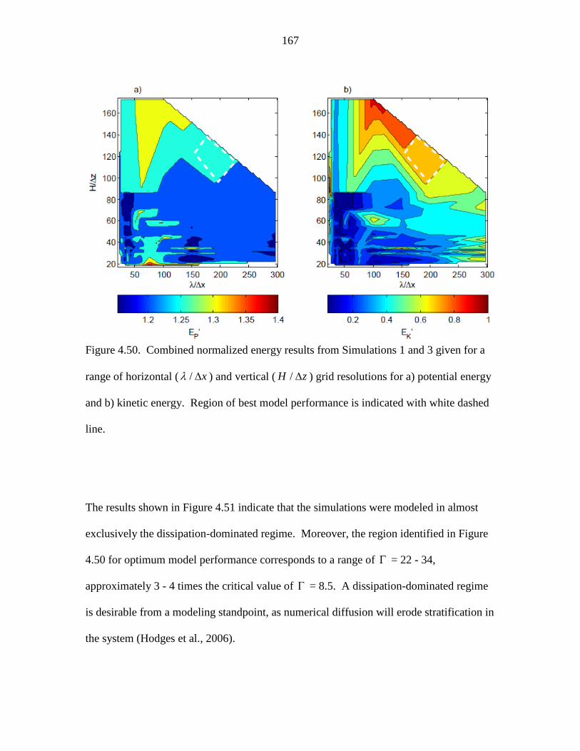
167
Figure 4.50. Combined normalized energy results from Simulations 1 and 3 given for a
range of horizontal ( / x ) and vertical ( /H z ) grid resolutions for a) potential energy
and b) kinetic energy. Region of best model performance is indicated with white dashed
line.
The results shown in Figure 4.51 indicate that the simulations were modeled in almost
exclusively the dissipation-dominated regime. Moreover, the region identified in Figure
4.50 for optimum model performance corresponds to a range of = 22 - 34,
approximately 3 - 4 times the critical value of = 8.5. A dissipation-dominated regime
is desirable from a modeling standpoint, as numerical diffusion will erode stratification in
the system (Hodges et al., 2006).
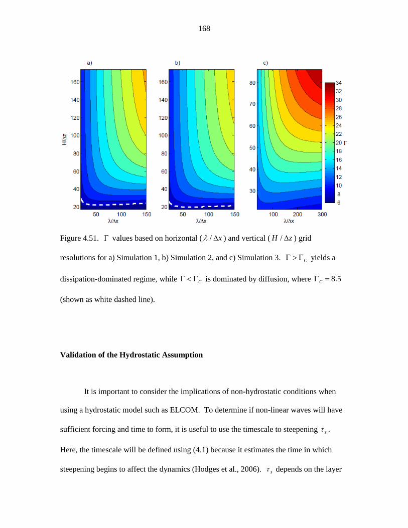
168
Figure 4.51. values based on horizontal ( / x ) and vertical ( /H z ) grid
resolutions for a) Simulation 1, b) Simulation 2, and c) Simulation 3. C yields a
dissipation-dominated regime, while C is dominated by diffusion, where 8.5C
(shown as white dashed line).
Validation of the Hydrostatic Assumption
It is important to consider the implications of non-hydrostatic conditions when
using a hydrostatic model such as ELCOM. To determine if non-linear waves will have
sufficient forcing and time to form, it is useful to use the timescale to steepening s .
Here, the timescale will be defined using (4.1) because it estimates the time in which
steepening begins to affect the dynamics (Hodges et al., 2006). s depends on the layer

169
Table 4.6. Parameters used to estimate steepening timescale s . Values are given for a
two-layer model with upper layer thickness 1h , bottom layer thickness 2h , wave
amplitude 0 , and period T . Results given for Simulations 1, 2 and 3.
Simulation h 1 (m) h 2 (m) ζ 0 (m) T (h) τ s (h)
1 6.15 11.25 0.2 1.3 13
2 6.4 11 0.4 1.5 8
3 14 29 4 13 14
thicknesses, the initial wave amplitude, and the period of the gravest (V1H1) mode
seiche. To estimate the steepening timescale, a two-layer approximation is made for the
thermal structures shown in Figures 4.9 for Simulations 1 and 2, and 4.36 for Simulation
3. To determine if non-linear conditions will occur, an isotherm near the center of the
thermocline was interpolated from field data and model output; the 17°C isotherm was
chosen for Simulations 1 and 2 , and the 18.5°C was chosen for Simulation 3. See Table
4.6 for parameters used to estimate s .
The time to steepening for all three simulations is shown based on an isotherm
displacement (Fig. 4.52). The results for Simulation 1 (Fig. 4.52a) show two time
periods where the 17°C isotherm is displaced approximately 0.2 m. This vertical
displacement, combined with the two-layer structure given in Table 4.6 yields steepening
time of approximately 13 h, ten times larger than the V1H1 period. ELCOM accurately
predicted the vertical displacement of the isotherm both during and after both time
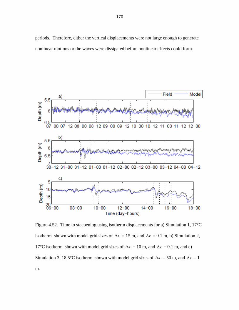
170
periods. Therefore, either the vertical displacements were not large enough to generate
nonlinear motions or the waves were dissipated before nonlinear effects could form.
Figure 4.52. Time to steepening using isotherm displacements for a) Simulation 1, 17°C
isotherm shown with model grid sizes of x = 15 m, and z = 0.1 m, b) Simulation 2,
17°C isotherm shown with model grid sizes of x = 10 m, and z = 0.1 m, and c)
Simulation 3, 18.5°C isotherm shown with model grid sizes of x = 50 m, and z = 1
m.

171
Figure 4.52b shows the isotherm depth for both field observations and model
predictions from Simulation 2. A large displacement was observed on 31 July the
amplitude of this displacement was used to determine s . The first vertical dashed line
indicates when the initial large-amplitude disturbance was observed; the second vertical
line is placed at time s later, indicating when steepening (if present) should have
occurred. The model predictions match field observations, except in not reproducing the
deep depression of the isotherm to approximately 6.7 m. In fact, the 17°C isotherm
begins to deepen in the afternoon of 1 August, well after nonlinear waves should have
been produced, and shows an almost steady decline.
Figure 4.52c shows the depth of the18.5 °C isotherm from both field and model
results from Simulation 3. Because of the more frequent low NL events experienced in
Simulation 3, three separate events during the 9, 14, and 15 July were isolated which
produced large amplitude displacements. Similarly, a pair of vertical lines is shown to
indicate the initial displacement and the time s later when steepening begins to become
important. The first large wind event on 9 July shows the position of the model isotherm
follows the same trend as seen in the field, but with a slight reduction in wave amplitude.
The second wind event on 14 July appears to be modeled even closer than the first; the
isotherm depth is matched almost exactly. However, the isotherm begins to deepen
shortly after the second wind event and ELCOM continues to overestimate the isotherm‘s
depth throughout the remainder of the simulation. During the third wind event the
overall trend in isotherm movement is well preserved and follows the measured behavior.

172
ELCOM was able to accurately predict the vertical isotherm displacement for all
simulations, indicating that either no nonlinear effects were present or nonlinear effects
were dissipated before a solitary wave could form. Thus, the use of the hydrostatic
assumption for modeling purposes is valid.
When considering the simulation time to the wave periods given in Table 4.6, it is
clear that simulations of Ada Hayden Lake for 5 d encompass approximately 80 wave
periods, while a 12 d simulation of West Okoboji Lake allows for approximately 22 wave
periods. Thus, while the longer simulation time of West Okoboji Lake is more than twice
as long as simulations of Ada Hayden Lake, it experiences approximately ¼ of the wave
oscillations. Therefore, simulation results can be related to the effects of either i) real
time or ii) wave period time.
Summary
Field work has shown the formation of internal waves for lakes of differing
characteristics. Because of strong stratification in Ada Hayden Lake during 2007 and
2008, winds of sufficient magnitude for large amplitude oscillations were sparse.
Conversely, West Okoboji Lake was less stratified and experience higher winds, resulting
in higher amplitude internal waves. Power spectra of isotherm displacement showed no
dominant waves were present during chosen time periods, merely a steady decrease in
power from low to high-frequency motions.
To conduct a grid resolution study of a three-dimensional, hydrostatic, numerical
model, ELCOM was used to simulate observed field conditions. Overall, it was shown

173
that ELCOM was able to reproduce wind-forced, basin-scale internal motions. Model
error was responsible for the deepening and thickening of the metalimnion, damping of
internal motions, and underestimating surface water temperature. Dimensionless energy
variables were used to quantify model performance in terms of retaining stratification and
reproducing water column response to environmental forcing.
For a hydrostatic model to provide accurate results, it is required that non-
hydrostatic forces be absent during a simulation. To address non-hydrostatic forces, a
two-layer model, combined with forcing conditions, was used to evaluate potential
internal wave degeneration mechanisms. These mechanisms can consist of basin-scale
internal waves or higher frequency flows such as billows and bores. Additionally, field
conditions appropriate for the formation of solitary waves were examined. All results
indicate that a hydrostatic model was capable of predicting internal waves.
Model results, dependent on horizontal and vertical cell grid sizes, were scaled to
combine measurements. These results varied between simulations from small horizontal
grid size and larger vertical grid size, to coarser horizontal resolution and finer vertical
resolution. Two simulated events of high and low internal wave activity were combined
to yield a range of model cell grid sizes where ELCOM was shown to provide numerical
results within 25% of field measurements. The model time step is related directly to the
horizontal grid size and the internal wave speed using a dimensionless number.

174
CHAPTER 5: CONCLUSIONS
Summary
Stratification in lakes and reservoirs has been shown to restrict and inhibit vertical
mixing and control the spatial variability of nutrients, dissolved oxygen, and other
dissolved substances. The energy flux path consists of momentum transfer from wind-
applied surface shear to the internal wave field, ultimately degenerating, dissipating, or
mixing. Internal dynamics within a stratified body therefore has far-reaching
implications in overall water quality and aquatic biological communities.
Numerical models play an important role in representing hydrodynamics in lakes
and coastal oceans. Three-dimensional models have been shown to accurately reproduce
thermal structures and circulation patterns. The coupling of physical models which solve
conservation equation with biological/chemical models provide new opportunities for the
use of numerical models outside the physical oceanography and limnology communities.
Much of success of 3D models has been well documented; however, the comparisons
made between real and simulated events (especially those of the internal wave field and
surface layer circulation) is often limited to qualitative discussion.
While 3D models have been shown to be accurate in predicting many facets of
hydrodynamic flows, numerical modeling is limited by the presence of numerical error:
numerical diffusion erodes stratification and numerical viscosity has been shown to
dampen and dissipate internal motions. Scaling has offered estimates for numerical
diffusion and dissipation, but these experiments were conducted on simplified basins with
175
simple waves. Therefore, by considering the effects of spatial and temporal resolution on
model predictions, this work evaluated the role of numerical error in model results
through comparison to field observations.
The methods for conducting field observations and the procedure for
implementing a three-dimensional hydrostatic model were presented. Also,
dimensionless energy variables were defined, which can be used to quantify and assess
model performance. Instrument locations were identified for three years of field work in
two lakes. Also, sampling strategy and explanations involved when planning field
studies were presented. Steps were presented which outline the necessary elements for a
successful simulation using the Estuary, Lake, and Coastal Ocean Model (ELCOM).
Field work showed the formation of internal waves for lakes of differing
characteristics. Because of strong stratification in Ada Hayden Lake during 2007 and
2008, winds of sufficient magnitude for large amplitude oscillations were sparse.
Conversely, West Okoboji Lake was less stratified and experienced higher winds,
resulting in larger amplitude internal waves. Power spectra of isotherm displacement
showed no dominant waves were present during chosen time periods, merely a steady
decrease in power from low to high-frequency motions.
To conduct a grid resolution study of a three-dimensional, hydrostatic, numerical
model, ELCOM was used to simulate observed field conditions. Overall, it was shown
that ELCOM was able to reproduce wind-forced, basin-scale internal motions. Model
error was responsible for the deepening and thickening of the metalimnion, damping of
internal motions, and underestimating surface water temperature. Dimensionless energy

176
variables were used to quantify model performance in terms of retaining stratification and
reproducing water column response to environmental forcing.
For a hydrostatic model to provide accurate results, it is required that non-
hydrostatic forces be absent during a simulation. To address non-hydrostatic forces, a
two-layer model, combined with forcing conditions, was used to evaluate potential
internal wave degeneration mechanisms. These mechanisms can consist of basin-scale
internal waves or higher frequency flows such as billows and bores. Additionally, field
conditions appropriate for the formation of solitary waves were examined. All results
indicate that a hydrostatic model was capable of predicting internal waves.
Model results, dependent on horizontal and vertical cell grid sizes, were scaled to
combine measurements. These results varied between simulations from small horizontal
grid size and larger vertical grid size, to coarser horizontal resolution and finer vertical
resolution. Two simulated events of high and low internal wave activity were combined
to yield a range of model cell grid sizes where ELCOM was shown to provide numerical
results within 25% of field measurements. The model time step is related directly to the
horizontal grid size and the internal wave speed using a dimensionless number.
Recommendations
Based on the discussion and results previously presented, the following
recommendations are made:
177
1. Internal waves have been observed in two Iowa lakes: Ada Hayden Lake and
West Okoboji Lake. Field measurements at high sampling frequency (15 s) were
capable of providing accurate observations of the internal lake response.
Additionally, these measurements were used to provide initial and forcing
conditions in a three-dimensional numerical model.
2. Degeneration mechanisms and steepening times were used to assess the validity
of the hydrostatic assumption in a model. Field observations and model results
supported the use of a hydrostatic model: nonlinear effects did not adversely
affect model results.
3. Model predictions at various grid sizes were able to predict basin-scale motions
under environmental forcing. Baroclinic motions—such as internal wave
propagation—were reproduced by the model.
4. Model results were evaluated in terms of potential and kinetic energies, and
isotherm displacement power spectra were used to evaluate whether vertical
oscillations were being produced over the entire frequency spectrum.
Comparisons of potential energy evaluated the model‘s ability to correctly predict
the vertical temperature structure in the lake, which depends on mixing, surface
heat fluxes, surface shear, and a conservative numerical scheme. Comparisons of
kinetic energy provided a method for assessing whether vertical motions predicted
by the model were comparable to field observations.
5. Model predictions were not invariant to the grid size chosen: smaller grid cell
sizes typically gave results closer to field observations. Scaling the model results
by the V1H1 wavelength and total depth H yielded a region where potential
178
and kinetic energies were within 25% of observed values. This region was
identified as / x = 150-225 and /H z = 95-140, encompasses the region
with the highest horizontal and vertical resolutions tested. Therefore, the
hypothesis that a refined model grid yields the best results is supported.
Future Work
The need for further research related to three-dimensional modeling is vast.
However, three areas of interest are immediately apparent. The first area of future work
is to relate the effects of the duration of a simulation event. Here, two time frames were
chosen for different lakes. As shown, the real time for West Okoboji Lake was longer
than either of the Ada Hayden Lake simulations, but it encompassed far fewer internal
wave oscillations. Additionally, the model time step was governed by the CFL number;
all simulated events were run with a fixed CFL value of 1/3. Further work could relate
the effects of the time step on model results.
The second area for future work is to use ELCOM to test the effects of wind
duration on internal response. Field results indicate that lower magnitude winds of longer
duration may yield larger amplitude oscillations than stronger winds of shorter duration.
ELCOM has the ability to predict flow conditions under a wide assortment of forcing
conditions; therefore, it can be used as a tool to test the effects of wind duration on
internal motions. Additionally, the layered analytical model presented can be used in
conjunction with a three-dimensional numerical model when comparing results.

179
The final item relates to the use of ELCOM in analyzing tracer study results.
Tracer studies have been conducted which track intrusions generated by boundary
mixing. ELCOM can be used to simulate advective transport in a tracer study. The
results from model simulations can be compared to field observations to determine if
small-scale mechanisms (which cannot be resolved by ELCOM) are responsible for the
intrusion.
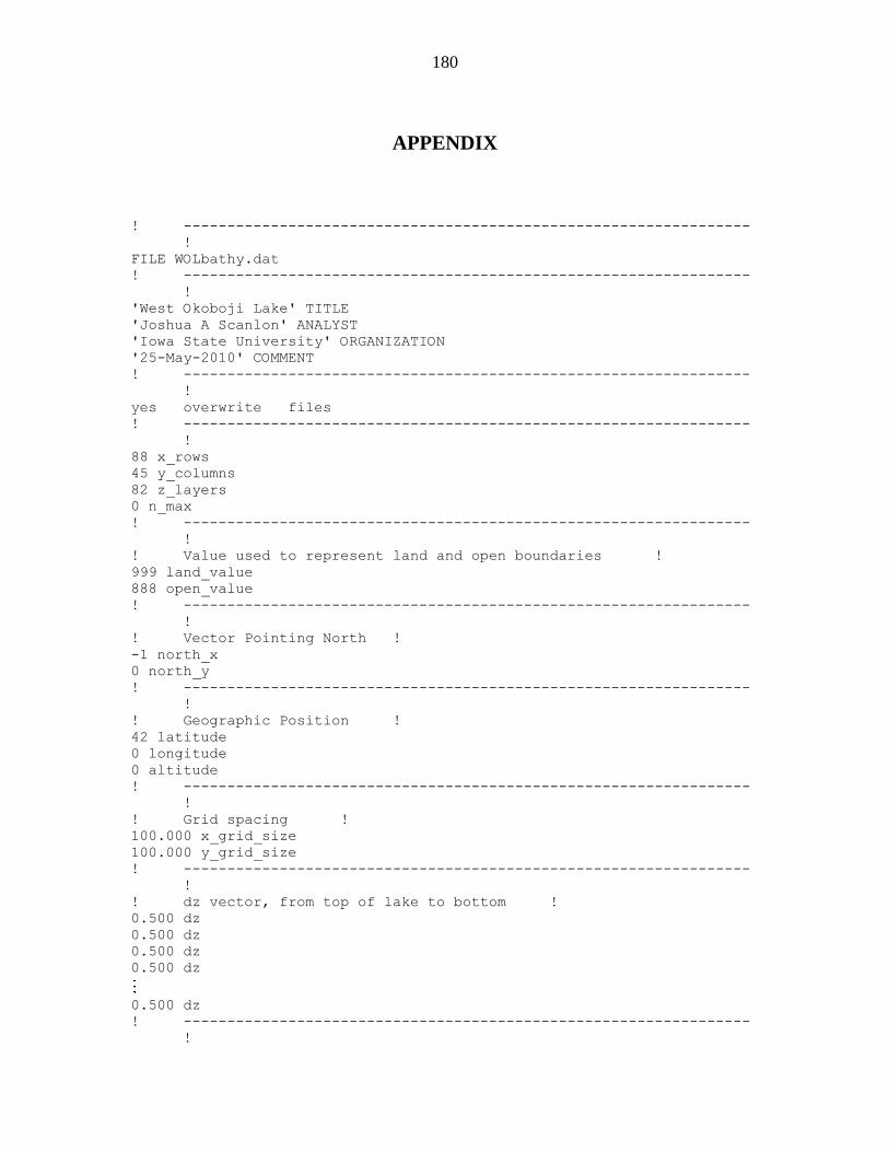
180
APPENDIX
! -----------------------------------------------------------------
!
FILE WOLbathy.dat
! -----------------------------------------------------------------
!
'West Okoboji Lake' TITLE
'Joshua A Scanlon' ANALYST
'Iowa State University' ORGANIZATION
'25-May-2010' COMMENT
! -----------------------------------------------------------------
!
yes overwrite files
! -----------------------------------------------------------------
!
88 x_rows
45 y_columns
82 z_layers
0 n_max
! -----------------------------------------------------------------
!
! Value used to represent land and open boundaries !
999 land_value
888 open_value
! -----------------------------------------------------------------
!
! Vector Pointing North !
-1 north_x
0 north_y
! -----------------------------------------------------------------
!
! Geographic Position !
42 latitude
0 longitude
0 altitude
! -----------------------------------------------------------------
!
! Grid spacing !
100.000 x_grid_size
100.000 y_grid_size
! -----------------------------------------------------------------
!
! dz vector, from top of lake to bottom !
0.500 dz
0.500 dz
0.500 dz
0.500 dz
0.500 dz
! -----------------------------------------------------------------
!
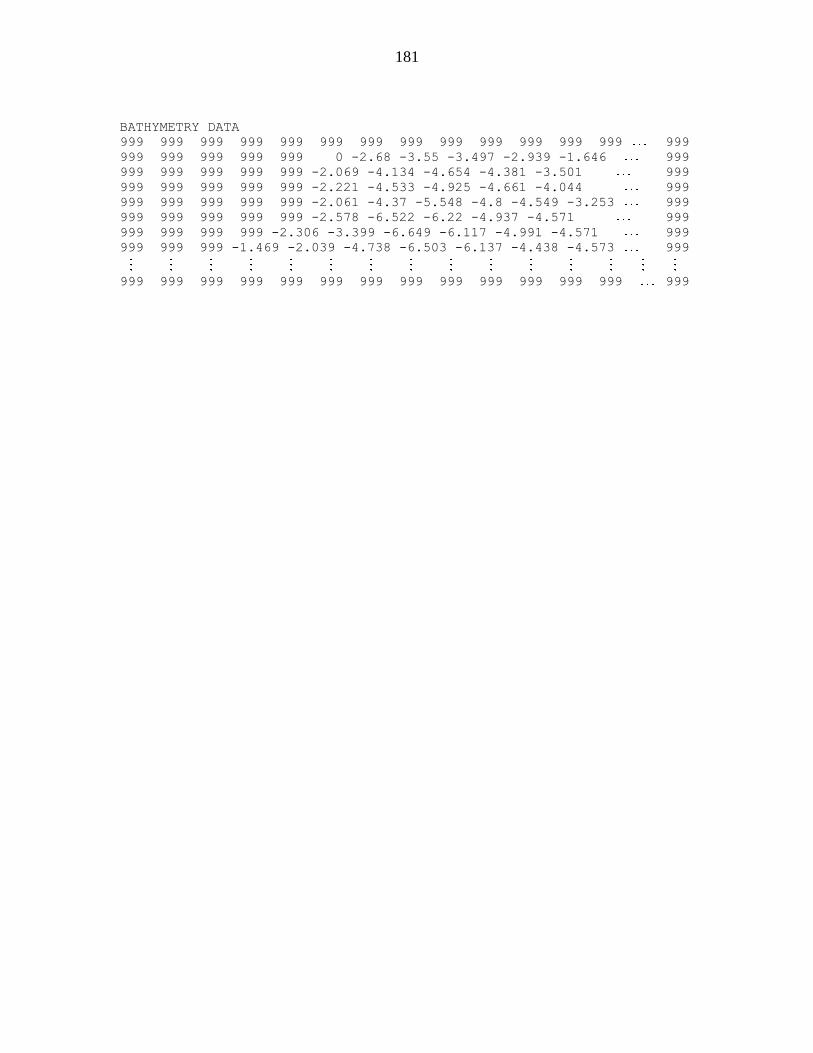
181
BATHYMETRY DATA
999 999 999 999 999 999 999 999 999 999 999 999 999 999
999 999 999 999 999 0 -2.68 -3.55 -3.497 -2.939 -1.646 999
999 999 999 999 999 -2.069 -4.134 -4.654 -4.381 -3.501 999
999 999 999 999 999 -2.221 -4.533 -4.925 -4.661 -4.044 999
999 999 999 999 999 -2.061 -4.37 -5.548 -4.8 -4.549 -3.253 999
999 999 999 999 999 -2.578 -6.522 -6.22 -4.937 -4.571 999
999 999 999 999 -2.306 -3.399 -6.649 -6.117 -4.991 -4.571 999
999 999 999 -1.469 -2.039 -4.738 -6.503 -6.137 -4.438 -4.573 999
999 999 999 999 999 999 999 999 999 999 999 999 999 999

182
FILE run_pre.dat
!-------------------------------------------------------!
! input files !
!-------------------------------------------------------!
! !
'bathymetry/WOLbathy.dat' BATHYMETRY_FILE
'bathymetry/WOLBC.dat' BOUNDARY_CONDITION_FILE
'bathymetry/WOLupdate.dat' UPDATE_FILE
!-------------------------------------------------------!
! output files !
!-------------------------------------------------------!
! !
'bathymetry/WOLout.txt' DATAOUT_FILE
'../run/infiles/usedata.unf' ELCOM_USEDATA_FILE
'../run/infiles/sparsedata.unf' ELCOM_SPARSEDATA_FILE
!-------------------------------------------------------!
! Permission to overwrite existing files !
yes overwrite
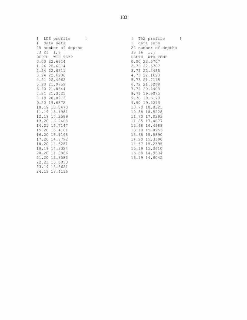
183
! LDS profile !
1 data sets
25 number of depths
73 23 i,j
DEPTH WTR_TEMP
0.00 22.6814
1.26 22.6814
2.24 22.6511
3.24 22.6206
4.21 22.4262
5.20 21.9759
6.20 21.8644
7.21 21.3021
8.19 20.0913
9.20 19.6372
10.19 18.8473
11.19 18.1981
12.19 17.2589
13.20 16.2468
14.21 15.7147
15.20 15.4161
16.20 15.1198
17.20 14.8792
18.20 14.6281
19.19 14.3324
20.20 14.0866
21.20 13.8583
22.21 13.6833
23.19 13.5621
24.19 13.4136
! T52 profile !
1 data sets
22 number of depths
33 16 i,j
DEPTH WTR_TEMP
0.00 22.5707
2.76 22.5707
3.73 22.4485
4.73 22.1623
5.73 21.7115
6.72 21.3268
7.72 20.2403
8.71 19.9075
9.70 19.6170
9.90 19.5213
10.70 18.8321
10.88 18.5228
11.70 17.9293
11.85 17.4877
12.68 16.4988
13.18 15.8253
13.68 15.5890
14.20 15.3390
14.67 15.2395
15.19 15.0610
15.68 14.9634
16.19 14.8045
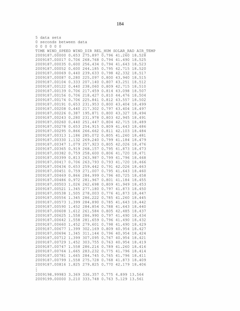
184
5 data sets
0 seconds between data
0 0 0 0 0 0
TIME WIND_SPEED WIND_DIR REL_HUM SOLAR_RAD AIR_TEMP
2009187.00000 0.653 275.897 0.796 41.260 18.528
2009187.00017 0.706 268.768 0.794 41.490 18.525
2009187.00035 0.600 256.434 0.794 41.643 18.523
2009187.00052 0.600 244.185 0.795 42.715 18.520
2009187.00069 0.440 239.633 0.798 42.332 18.517
2009187.00087 0.280 225.097 0.800 43.940 18.515
2009187.00104 0.333 207.140 0.807 43.251 18.512
2009187.00122 0.440 238.060 0.809 42.715 18.510
2009187.00139 0.706 217.459 0.814 43.098 18.507
2009187.00156 0.706 218.427 0.810 44.476 18.504
2009187.00174 0.706 225.841 0.812 43.557 18.502
2009187.00191 0.653 231.953 0.800 43.404 18.499
2009187.00208 0.440 217.302 0.797 43.404 18.497
2009187.00226 0.387 195.871 0.800 43.327 18.494
2009187.00243 0.280 231.978 0.803 42.945 18.491
2009187.00260 0.440 251.447 0.804 42.715 18.489
2009187.00278 0.653 254.915 0.809 41.643 18.486
2009187.00295 0.866 266.662 0.811 42.103 18.484
2009187.00313 1.186 285.072 0.805 41.260 18.481
2009187.00330 1.132 269.240 0.799 41.184 18.479
2009187.00347 1.079 257.923 0.805 42.026 18.476
2009187.00365 0.919 268.157 0.795 41.873 18.473
2009187.00382 0.759 258.600 0.806 41.720 18.471
2009187.00399 0.813 263.987 0.799 41.796 18.468
2009187.00417 0.706 263.793 0.793 41.720 18.466
2009187.00434 0.653 259.442 0.791 42.026 18.463
2009187.00451 0.759 271.007 0.795 41.643 18.460
2009187.00469 0.866 284.999 0.796 40.725 18.458
2009187.00486 0.972 281.967 0.801 41.184 18.455
2009187.00503 1.026 262.698 0.809 41.949 18.453
2009187.00521 1.345 277.180 0.797 41.873 18.450
2009187.00538 1.505 278.003 0.776 41.873 18.447
2009187.00556 1.345 286.222 0.785 41.260 18.445
2009187.00573 1.399 284.890 0.785 41.643 18.442
2009187.00590 1.452 284.854 0.788 41.643 18.440
2009187.00608 1.612 261.584 0.805 42.485 18.437
2009187.00625 1.558 286.990 0.797 41.490 18.434
2009187.00642 1.558 281.659 0.796 41.490 18.432
2009187.00660 1.452 279.601 0.798 41.490 18.429
2009187.00677 1.399 302.169 0.809 40.954 18.427
2009187.00694 1.345 311.144 0.796 40.954 18.424
2009187.00712 1.399 307.095 0.767 40.954 18.421
2009187.00729 1.452 303.755 0.763 40.954 18.419
2009187.00747 1.558 286.216 0.789 41.260 18.416
2009187.00764 1.665 283.232 0.775 41.796 18.414
2009187.00781 1.665 284.745 0.765 41.796 18.411
2009187.00799 1.558 275.728 0.768 41.873 18.409
2009187.00816 1.825 279.825 0.770 42.179 18.406
2009198.99983 3.369 336.357 0.775 4.899 13.564
2009199.00000 3.210 333.748 0.763 5.129 13.561

185
DATABLOCK DESCRIPTION FILE
1.1.a ! datablock version
2 ! number of output groups
2 ! number of output sets
BEGIN GROUP_DESCRIPTION
001 ! group reference number
tc52_grp ! user label
tc52_prof.unf ! output filename
001 ! set reference number
4 ! number of datatypes in group
.TRUE. ! is_interval? logical: true if time step
interval is used for output
36 ! output interval
0 ! output start time
0 ! output end time, 0 indicates entire run
0 ! size of time list, non-zero only if
is_interval = .FALSE.
BEGIN GROUP_DESCRIPTION
002 ! group reference number
lds_grp ! user label
lds_prof.unf ! output filename
002 ! set reference number
4 ! number of datatypes in group
.TRUE. ! is_interval? logical: true if time step
interval is used for output
36 ! output interval
0 ! output start time
0 ! output end time, 0 indicates entire run
0 ! size of time list, non-zero only if
is_interval = .FALSE.
BEGIN SET_DESCRIPTION
001 ! set reference number
tc52_set ! user label
PROFILE_1D ! type of set
1 ! number of cells in set
NULL ! sheet type
NULL ! sheet calc
1.0 ! sheet value
NULL ! dynamic name #1
NULL ! dynamic calc #1
NULL ! dynamic direction #1
0.0 ! dynamic value #1
NULL ! dynamic name #2
NULL ! dynamic calc #2
NULL ! dynamic direction #2
0.0 ! dynamic value #2
BEGIN SET_DESCRIPTION
002 ! set reference number
lds_set ! user label
PROFILE_1D ! type of set
1 ! number of cells in set
NULL ! sheet type
NULL ! sheet calc
1.0 ! sheet value
NULL ! dynamic name #1
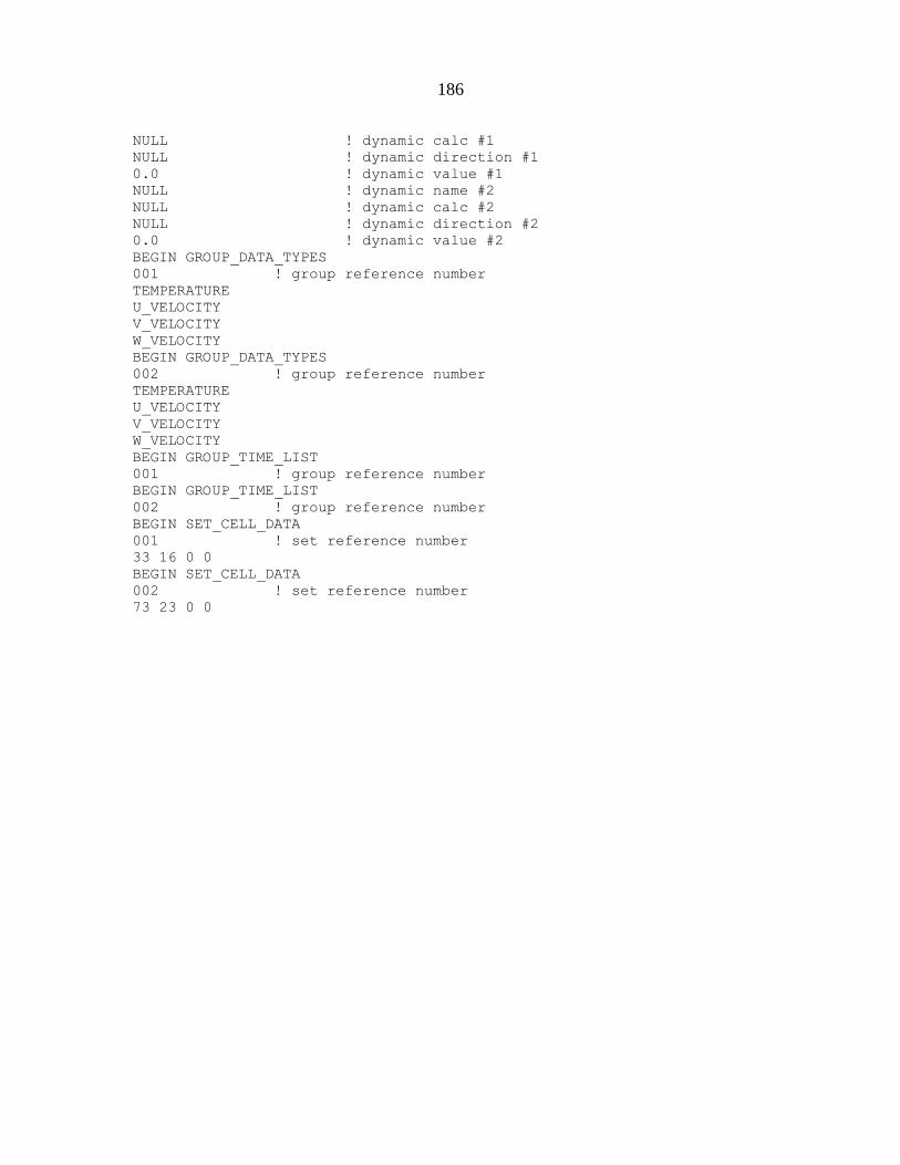
186
NULL ! dynamic calc #1
NULL ! dynamic direction #1
0.0 ! dynamic value #1
NULL ! dynamic name #2
NULL ! dynamic calc #2
NULL ! dynamic direction #2
0.0 ! dynamic value #2
BEGIN GROUP_DATA_TYPES
001 ! group reference number
TEMPERATURE
U_VELOCITY
V_VELOCITY
W_VELOCITY
BEGIN GROUP_DATA_TYPES
002 ! group reference number
TEMPERATURE
U_VELOCITY
V_VELOCITY
W_VELOCITY
BEGIN GROUP_TIME_LIST
001 ! group reference number
BEGIN GROUP_TIME_LIST
002 ! group reference number
BEGIN SET_CELL_DATA
001 ! set reference number
33 16 0 0
BEGIN SET_CELL_DATA
002 ! set reference number
73 23 0 0
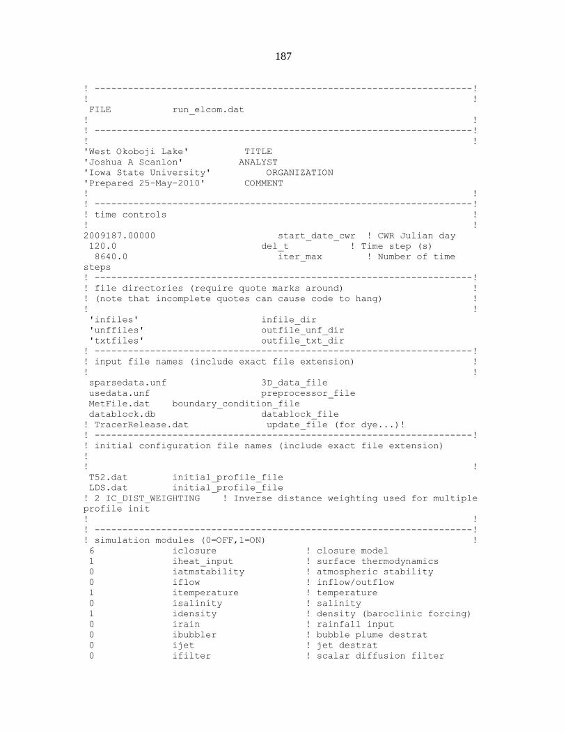
187
! --------------------------------------------------------------------!
! !
FILE run_elcom.dat
! !
! --------------------------------------------------------------------!
! !
'West Okoboji Lake' TITLE
'Joshua A Scanlon' ANALYST
'Iowa State University' ORGANIZATION
'Prepared 25-May-2010' COMMENT
! !
! --------------------------------------------------------------------!
! time controls !
! !
2009187.00000 start_date_cwr ! CWR Julian day
120.0 del_t ! Time step (s)
8640.0 iter_max ! Number of time
steps
! --------------------------------------------------------------------!
! file directories (require quote marks around) !
! (note that incomplete quotes can cause code to hang) !
! !
'infiles' infile_dir
'unffiles' outfile_unf_dir
'txtfiles' outfile_txt_dir
! --------------------------------------------------------------------!
! input file names (include exact file extension) !
! !
sparsedata.unf 3D_data_file
usedata.unf preprocessor_file
MetFile.dat boundary_condition_file
datablock.db datablock_file
! TracerRelease.dat update_file (for dye...)!
! --------------------------------------------------------------------!
! initial configuration file names (include exact file extension)
!
! !
T52.dat initial_profile_file
LDS.dat initial_profile_file
! 2 IC_DIST_WEIGHTING ! Inverse distance weighting used for multiple
profile init
! !
! --------------------------------------------------------------------!
! simulation modules (0=OFF,1=ON) !
6 iclosure ! closure model
1 iheat_input ! surface thermodynamics
0 iatmstability ! atmospheric stability
0 iflow ! inflow/outflow
1 itemperature ! temperature
0 isalinity ! salinity
1 idensity ! density (baroclinic forcing)
0 irain ! rainfall input
0 ibubbler ! bubble plume destrat
0 ijet ! jet destrat
0 ifilter ! scalar diffusion filter

188
0 iretention ! track retention time
0 ICAEDYM ! water quality module
1 icoriolis ! turn off/on coriolis forcing
0 ntracer ! number of tracers
! !
! --------------------------------------------------------------------!
! default boundary conditions !
! !
! 1 = noslip all !
! 2 = freeslip all !
! 3 = drag all !
! 4 = neumann all !
! 5 = slip sides, noslip bottom !
! 6 = slip sides, drag bottom !
! 7 = slip sides, neumann bottom !
! 8 = header values !
! 9 = turbulent benthic boundary layer !
! !
9 DEFAULT_BC
! --------------------------------------------------------------------!
! bottom drag
! !
0.005 drag_btm_cd
! --------------------------------------------------------------------!
! default values (superseded by inputs in elcom_setup.f90) !
! !
2.14 WIND_SPEED_HEIGHT ! Wind sensor height
2.14 SCALAR_HEIGHT ! Met sensor height
! --------------------------------------------------------------------!
! default values (superseded by inputs in elcom_setup.f90) !
! !
0.0 DEFAULT_HEIGHT ! Initial uniform water level
20.0 DEFAULT_WTR_TEMP ! Initial uniform temperature
0.0 DEFAULT_TRACER_1 ! Initial uniform tracer
0.0 DEFAULT_WIND_SPEED ! Uniform wind speed
0.0 DEFAULT_WIND_DIR ! Uniform wind direction
0.25 DEFAULT_PAR_EXTINCTION ! PAR extinction coefficient
45% of SW
1.00 DEFAULT_NIR_EXTINCTION ! NIR extinction coefficient
41% of SW
1.00 DEFAULT_UVA_EXTINCTION ! UVA extinction coefficient
3.5% of SW
2.50 DEFAULT_UVB_EXTINCTION ! UVB extinction coefficient
0.5% of SW
0.08 mean_albedo !
! !
! --------------------------------------------------------------------!
! horizontal diffusivities !
! !
0.0 DEFAULT_DIFFUSIVITY ! Default horizontal
diffusivity for all scalars
! !
! --------------------------------------------------------------------!
'NONE' CASE_KEYWORD
! !
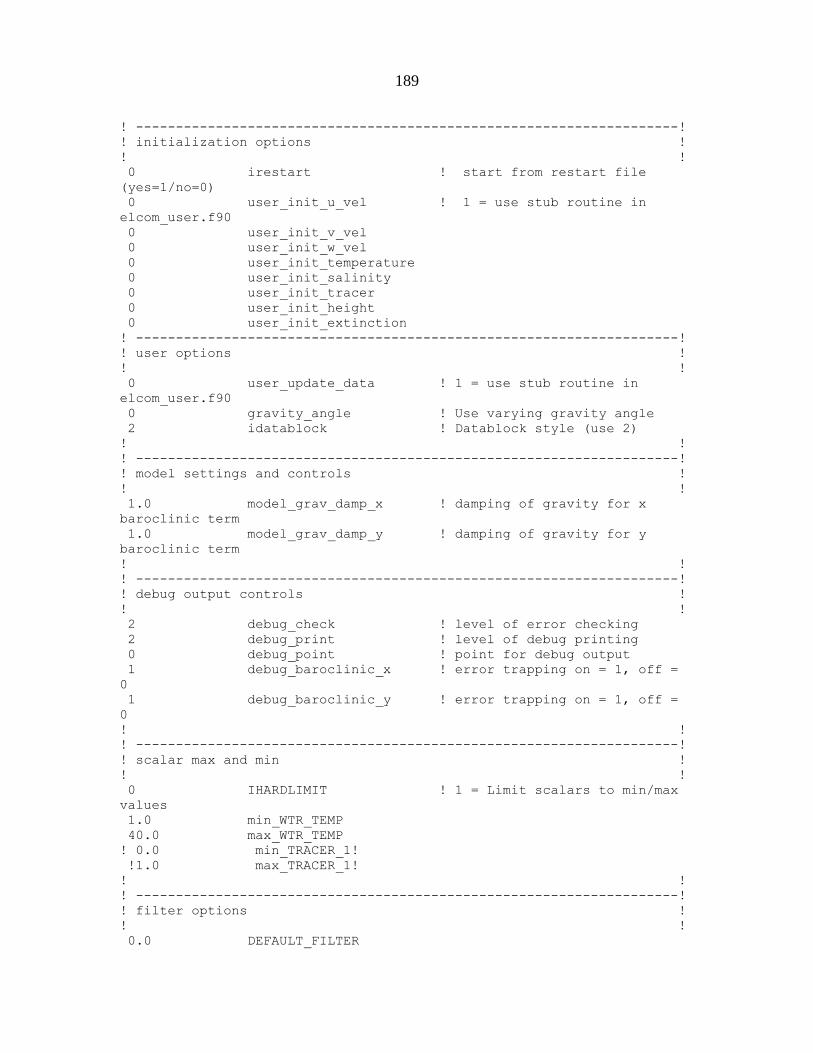
189
! --------------------------------------------------------------------!
! initialization options !
! !
0 irestart ! start from restart file
(yes=1/no=0)
0 user_init_u_vel ! 1 = use stub routine in
elcom_user.f90
0 user_init_v_vel
0 user_init_w_vel
0 user_init_temperature
0 user_init_salinity
0 user_init_tracer
0 user_init_height
0 user_init_extinction
! --------------------------------------------------------------------!
! user options !
! !
0 user_update_data ! 1 = use stub routine in
elcom_user.f90
0 gravity_angle ! Use varying gravity angle
2 idatablock ! Datablock style (use 2)
! !
! --------------------------------------------------------------------!
! model settings and controls !
! !
1.0 model_grav_damp_x ! damping of gravity for x
baroclinic term
1.0 model_grav_damp_y ! damping of gravity for y
baroclinic term
! !
! --------------------------------------------------------------------!
! debug output controls !
! !
2 debug_check ! level of error checking
2 debug_print ! level of debug printing
0 debug_point ! point for debug output
1 debug_baroclinic_x ! error trapping on = 1, off =
0
1 debug_baroclinic_y ! error trapping on = 1, off =
0
! !
! --------------------------------------------------------------------!
! scalar max and min !
! !
0 IHARDLIMIT ! 1 = Limit scalars to min/max
values
1.0 min_WTR_TEMP
40.0 max_WTR_TEMP
! 0.0 min_TRACER_1!
!1.0 max_TRACER_1!
! !
! --------------------------------------------------------------------!
! filter options !
! !
0.0 DEFAULT_FILTER
190
! !
! --------------------------------------------------------------------!
! frequency of outputs !
! !
50 iter_out_monitor ! monitoring output to screen
5000 iter_out_save ! saving separate restart files
1000 iter_out_restart ! overwriting restart output!
! !
! --------------------------------------------------------------------!
! start of outputs !
! !
0 start_output_monitor ! monitor output to screen
0 start_output_save ! saved restart files
! !
! --------------------------------------------------------------------!
! conjugate gradient iteration controls !
! !
1.e-16 CGM_TOL ! CGM tolerance
30 CGM_MIN ! minimum iterations of CGM
1000 CGM_MAX ! maximum iterations of CGM
! !
! --------------------------------------------------------------------!
! restart file names (do not include file extension) !
! !
save restart_save_file
restart_final restart_out_file
191
! Profile translation
lds_prof.unf
../infiles/sparsedata.unf
../ncfiles/profile_LDS.nc
-1
-1
clobber !replace
no_map
no_echo
! Profile translation
tc52_prof.unf
../infiles/sparsedata.unf
../ncfiles/profile_TC52.nc
-1
-1
clobber !replace
no_map
no_echo
192
REFERENCES
Antenucci, J. P., J. Imberger, and A. Saggio. 2000. Seasonal evolution of the basin-scale
internal wave field in a large stratified lake. Limnol. Oceanogr. 45: 1621-1638.
Beletsky, D., W. P. Oconnor, D. J. Schwab, and D. E. Dietrich. 1997. Numerical
simulation of internal Kelvin waves and coastal upwelling fronts. J. Phys.
Oceanogr. 27: 1197-1215.
Boegman, L., G. N. Ivey, and J. Imberger. 2005. The energetics of large-scale internal
wave degeneration in lakes. J. Fluid Mech. 531: 159-180.
Botelho, D., J. Imberger, C. Dallimore, and B. R. Hodges. 2009. A hydrostatic/non-
hydrostatic grid-switching strategy for computing high-frequency, high wave
number motions embedded in geophysical flows. Environ. Modell. Softw. 24:
473-488.
Botelho, D. A., and J. Imberger. 2007. Downscaling model resolution to illuminate the
internal wave field in a small stratified lake. J. Hydraul. Eng. 133: 1206-1218.
Casulli, V., and R. T. Cheng. 1992. Semi-implicit finite-difference methods for 3-
dimensional shallow-water flow. International Journal for Numerical Methods in
Fluids 15: 629-648.
Chung, S. W., M. R. Hipsey, and J. Imberger. 2009. Modelling the propagation of turbid
density inflows into a stratified lake: Daecheong Reservoir, Korea. Environ.
Modell. Softw. 24: 1467-1482.
Csanady, G. T. 1982. On the structure of transient upwelling events. J. Phys. Oceanogr.
12: 84-96.
Cushman-Roisin, B. 1994. Introduction to Geophysical Fluid Dynamics. Prentice-Hall.
Eckert, W., J. Imberger, and A. Saggio. 2002. Biogeochemical response to physical
forcing in the water column of a warm monomictic lake. Biogeochemistry 61:
291-307.
Fee, E. J. 1967. The seiches of Lake West Okoboji. Iowa State J. Sci. 42: 73-81.
Fee, E. J., and R. W. Bachmann. 1968. An empirical study of Defant method of seiche
analysis. Limnol. Oceanogr. 13: 665-&.
Gill, A. E. 1982. Atmosphere-Ocean Dynamics. Academic Press.
Gomez-Giraldo, A., J. Imberger, and J. P. Antenucci. 2006. Spatial structure of the
dominant basin-scale internal waves in Lake Kinneret. Limnol. Oceanogr. 51:
229-246.
193
Heaps, N. S., and A. E. Ramsbottom. 1966. Wind effects on water in a narrow two-
layered lake. Philosophical Transactions of the Royal Society of London Series
A-Mathematical and Physical Sciences 259: 391-&.
Hodges, B.R. 2000. Numerical techniques in CWR-ELCOM. Technical Report WP
1422 BH, Centre for Water Research, University of Western Australia.
Hodges, B. R., and C. Dallimore. 2007. Estuary, Lake and Coastal Ocean Model:
ELCOM. Version 2.2: User's manual. Centre for Water Research, University of
Western Australia.
Hodges, B. R., J. Imberger, A. Saggio, and K. B. Winters. 2000. Modeling basin-scale
internal waves in a stratified lake. Limnol. Oceanogr. 45: 1603-1620.
Hodges, B. R., B. Laval, and B. M. Wadzuk. 2006. Numerical error assessment and a
temporal horizon for internal waves in a hydrostatic model. Ocean Model. 13: 44-
64.
Hodges, B. R., and F. J. Rueda. 2008. Semi-implicit two-level predictor-corrector
methods for non-linearly coupled, hydrostatic, barotropic/baroclinic flows.
International Journal of Computational Fluid Dynamics 22: 593-607.
Horn, D. A., J. Imberger, and G. N. Ivey. 2001. The degeneration of large-scale
interfacial gravity waves in lakes. J. Fluid Mech. 434: 181-207.
Imberger, J. 1994. Measurement of turbulent properties in a natural system, p. 1-20. In C.
A. Pugh [ed.], Fundamentals and Advancements in Hydraulic Measurements and
Experimentation.
Imberger, J. 1998. Flux paths in a stratified lake: a review, p. 1-18. In J. Imberger [ed.],
Physical Processes in Lakes and Oceans. Coastal and Estuarine Studies. American
Geophysical Union.
Imberger, J. 2004. Characterizing the dynamical regimes of a lake, p. 1121-1130. In A.
H. El-Shaarawi [ed.], The Encyclopaedia of Environmetrics. Wiley.
Imberger, J., and J. C. Patterson. 1981. A dynamic reservoir simulation model—
DYRESM 5, p. 310-361. In H. Fisher [ed.], Transport models for inland and
coastal waters. Academic Press.
Imberger, J., and J.C. Patterson. 1990. Physical limnology. Advances in Applied
Mechanics 27: 303-475.
Kalff, J. 2002. Limnology. Prentice-Hall.
Kocyigit, M. B., and R. A. Falconer. 2004. Three-dimensional numerical modelling of
wind-driven circulation in a homogeneous lake. Advances in Water Resources 27:
1167-1178.

194
Kundu, P. K., and I. M. Cohen. 2008. Fluid Mechanics. Academic Press.
Laval, B., B. R. Hodges, and J. Imberger. 2003a. Reducing numerical diffusion effects
with pycnocline filter. J. Hydraul. Eng. 129: 215-224.
Laval, B., J. Imberger, B. R. Hodges, and R. Stocker. 2003b. Modeling circulation in
lakes: Spatial and temporal variations. Limnol. Oceanogr. 48: 983-994.
Laval, B. E., J. Imberger, and A. N. Findikakis. 2005. Dynamics of a large tropical lake:
Lake Maracaibo. Aquatic Sciences 67: 337-349.
Lemckert, C., and J. Imberger. 1998. Turbulent benthic boundary layer mixing events in
fresh water lakes, p. 503-516. In J. Imberger [ed.], Physical Processes in Lakes in
Oceans. Coastal and Estuarine Studies.
Leon, L. K., J. Imberger, R. E. H. Smith, R. E. Hecky, D. C. L. Lam, and W. M.
Schertzer. 2005. Modeling as a tool for nutrient management in Lake Erie: a
hydrodynamics study. Journal of Great Lakes Research 31: 309-318.
Leonard, B. P. 1991. The ULTIMATE conservative difference scheme applied to
unsteady one-dimensional advection. Computer Methods in Applied Mechanics
and Engineering 88: 17-74.
Lighthill, M. J. 1969. Dynamic response of the Indian Ocean to onset of the Southwest
Monsoon. Philosophical Transactions of the Royal Society of London Series A-
Mathematical and Physical Sciences 265: 45-92.
Liu, Y., P. MacCready, B. M. Hickey, E. P. Dever, P. M. Kosro, and N. S. Banas. 2009.
Evaluation of a coastal ocean circulation model for the Columbia River plume in
summer 2004. J. Geophys. Res. 114: C00B04.
Lorenz, E. N. 1955. Available potential energy and the maintenance of the general
circulation. Tellus 7: 157-167.
MacIntyre, S., K. M. Flynn, R. Jellison, and J. R. Romero. 1999. Boundary mixing and
nutrient fluxes in Mono Lake, California. Limnol. Oceanogr. 44: 512-529.
Marti-Cardona, B., T. E. Steissberg, S. G. Schladow, and S. J. Hook. 2008. Relating fish
kills to upwellings and wind patterns in the Salton Sea. Hydrobiologia 604: 85-95.
Monismith, S. G. 1985. Wind-forced motions in stratified lakes and their effect on
mixed-layer shear. Limnol. Oceanogr. 30: 771-783.
Moum, J. N., and J. D. Nash. 2000. Topographically induced drag and mixing at a small
bank on the continental shelf. J. Phys. Oceanogr. 30: 2049-2054.
Münnich, M., A. Wüest, and D. M. Imboden. 1992. Observations of the second vertical
mode of the internal seiche in an alpine lake. Limnol. Oceanogr. 37: 1705-1719.

195
Pedlosky, J. 1979. Geophysical Fluid Dynamics. Springer.
Rao, Y. R., C. H. Marvin, and J. Zhao. 2009. Application of a numerical model for
circulation, temperature and pollutant distribution in Hamilton Harbour. Journal
of Great Lakes Research 35: 61-73.
Rueda, F. J., E. Sanmiguel-Rojas, and B. R. Hodges. 2007. Baroclinic stability for a
family of two-level, semi-implicit numerical methods for the 3D shallow water
equations. International Journal for Numerical Methods in Fluids 54: 237-268.
Saggio, A., and J. Imberger. 1998. Internal wave weather in a stratified lake. Limnol.
Oceanogr. 43: 1780-1795.
Saggio, A., and J. Imberger. 2001. Mixing and turbulent fluxes in the metalimnion of a
stratified lake. Limnol. Oceanogr. 46: 392-409.
Simanjuntak, M. A., J. Imberger, and K. Nakayama. 2009. Effect of stair-step and
piecewise linear topography on internal wave propagation in a geophysical flow
model. J. Geophys. Res.-Oceans 114.
Smith, S. D. 1988. Coefficients for sea surface wind stress, heat flux, and wind profiles as
a function of wind speed and temperature. Journal of Geophysical Research 93:
15467-15472.
Spigel, R. H., and J. Imberger. 1980. The classification of mixed-layer dynamics in lakes
of small to medium size. J. Phys. Oceanogr. 10: 1104-1121.
Spigel, R. H., J. Imberger, and K. N. Rayner. 1986. Modeling the diurnal mixed layer.
Limnol. Oceanogr. 31: 533-556.
Spillman, C. M., J. Imberger, D. P. Hamilton, M. R. Hipsey, and J. R. Romero. 2007.
Modelling the effects of Po River discharge, internal nutrient cycling and
hydrodynamics on biogeochemistry of the Northern Adriatic Sea. Journal of
Marine Systems 68: 167-200.
Stevens, C., G. Lawrence, P. Hamblin, and E. Carmack. 1996. Wind forcing of internal
waves in a long narrow stratified lake. Dyn. Atmos. Oceans 24: 41-50.
Stevens, C. L., and G. A. Lawrence. 1997. Estimation of wind-forced internal seiche
amplitudes in lakes and reservoirs, with data from British Columbia, Canada.
Aquatic Sciences 59: 115-134.
Thompson, R. O., and J. Imberger. 1980. Response of a numerical model of a stratified
lake to wind stress, p. 562-570. 2nd International Symposium on Stratified Flows.
Turner, J. S. 1973. Buoyancy Effects in Fluids. Cambridge University Press.

196
Vidal, J., and X. Casamitjana. 2008. Forced resonant oscillations as a response to
periodic winds in a stratified reservoir. Journal of Hydraulic Engineering-Asce
134: 416-425.
Vidal, J., X. Casamitjana, J. Colomer, and T. Serra. 2005. The internal wave field in Sau
reservoir: Observation and modeling of a third vertical mode. Limnol. Oceanogr.
50: 1326-1333.
Wilkin, J. L. 2006. The summertime heat budget and circulation of southeast New
England shelf waters. J. Phys. Oceanogr. 36: 1997-2011.
Willmott, C. J. 1981. On the validation of models. Phys. Geogr. 2: 184-194.
Willmott, C. J. 1982. Some comments on the evaluation of model performance.
Willmott, C. J., and D. E. Wicks. 1980. An empirical method for the spatial interpolation
of monthly precipitation within California. Phys. Geogr. 1: 59-73.
Winters, K. B., P. N. Lombard, J. J. Riley, and E. A. D'Asaro. 1995. Available potential
energy and mixing in density-stratified fluids. J. Fluid Mech. 289: 115-128.
Wüest, A., and A. Lorke. 2003. Small-scale hydrodynamics in lakes. Annu. Rev. Fluid
Mech. 35: 373-412.
Yeates, P. S., J. Imberger, and C. Dallimore. 2008. Thermistor chain data assimilation to
improve hydrodynamic modeling skill in stratified lakes and reservoirs. J.
Hydraul. Eng. 134: 1123-1135.
Yelland, M., and P. K. Taylor. 1996. Wind stress measurements from the open ocean. J.
Phys. Oceanogr. 26: 541-558.
Copyright © 2022 FDOKUMEN