
Modeling energy and carbon fluxes in a heterogeneous oak woodland: A three-dimensional approach
18
Agricultural and Forest Meteorology 152 (2012) 83–100 Contents lists available at SciVerse ScienceDirect Agricultural and Forest Meteorology jou rn al h om epa g e: www.elsevier.com/locate/agrformet Modeling energy and carbon fluxes in a heterogeneous oak woodland: A three-dimensional approach Hideki Kobayashi a,e,∗ , Dennis D. Baldocchi a , Youngryel Ryu b , Qi Chen c , Siyan Ma a , Jessica L. Osuna a , Susan L. Ustin d a Department of Environmental Science, Policy and Management, University of California, Berkeley, Berkeley 94720, CA, USA b Department of Organismic and Evolutionary Biology, Harvard University, Cambridge, MA, USA c Department of Geography, University of Hawai’i, Honolulu, HI, USA d Center for Spatial Technologies and Remote Sensing, University of California, Davis, CA, USA e Research Institute for Global Change, Japan Agency for Marine-Earth Science and Technology, 3173-25 Showa machi, Yokohama, Japan a r t i c l e i n f o Article history: Received 17 November 2010 Received in revised form 5 September 2011 Accepted 10 September 2011 Keywords: 3D radiative transfer Energy balance Eddy covariance Light environment Savanna woodland Model-data intercomparison a b s t r a c t Most land surface and ecosystem models assume that a vegetated canopy can be abstracted as a turbid medium when such models compute mass, energy, and carbon exchange. However, those models fail to simulate radiation environments in heterogeneous landscapes. This study aims to couple a spatially explicit three-dimensional (3D) shortwave and longwave radiative transfer model with a soil and canopy energy balance and canopy physiology model (CANOAK-FLiES), to investigate how well the 3D model performs in a heterogeneous landscape compared to a 1D model. The canopy structural parameters were extracted using airborne-based Light Detection and Ranging (LiDAR) data and digital cover photographs. The developed model was compared with a wide variety of field and remote sensing data (e.g., hyper- spectral remote sensing images, overstory and understory radiation, and tower-based energy and CO 2 fluxes) in a woody oak savanna in CA, USA. Overall, the simulated spatial and diurnal patterns of the radiation environment were consistent with the measurements of shortwave and longwave wavebands. The 3D approach worked better than the 1D approach from the wet mild spring to the dry hot summer while the relative importance of using the 3D approach depends on climate and canopy physiological conditions as well as the canopy structure. With low leaf area index in the oak woodland, the woody elements absorbed 12%–39% of the PAR and 20%–52% of the NIR radiation. Consequently, 12% of the daytime energy flux was used as woody heat storage at our study site. This novel 3D model has the potential to serve as a useful tool for analyzing the spatio-temporal variability of radiation and energy fluxes in evaluating footprints of radiation sensors and eddy covariance fluxes, and serve as a standard in evaluating the performance of a hierarchy of simpler land surface models to compute mass and energy exchange of heterogeneous landscapes. © 2011 Elsevier B.V. All rights reserved. 1. Introduction Most land surface and ecosystem models assume that a veg- etated canopy can be abstracted as a turbid medium to compute mass, energy, and carbon exchange. With this assumption, the canopy is horizontally homogeneous as leaves are randomly distributed in space. Consequently, radiation only changes in a vertical direction. This simplified modeling makes it difficult to evaluate the radiation environment in spatially heterogeneous landscapes such as savanna ecosystems (Sankaran et al., 2005; Scholes and Archer, 1997). In particular, the spatial separation ∗ Corresponding author at: Research Institute for Global Change, Japan Agency for Marine-Earth Science and Technology, 3173-25 Showa machi, Yokohama, Japan. E-mail address: [email protected] (H. Kobayashi). of individual tree crowns forms regions where beams of light travel without interactions with foliage and regions where light is strongly attenuated. This neglected spatial attribute in the turbid medium type models motivates us to challenge and critique the widely held assumption of a turbid medium. We aim to take a spa- tially explicit three-dimensional (3D) approach to understand the role of heterogeneous structure on the energy and carbon fluxes. The 3D approach requires more computation time and canopy structural variables than 1D turbid medium models. However, the 3D approach is expected to give more reliable energy and carbon fluxes when the reliable canopy structural variables are available. Also, airborne-Light Detection and Ranging (LiDAR) data has been retrieved in many areas, thus it is expected that more LiDAR data would be available in the near future. Therefore, the 3D model can fill the theoretical gap between 1D models and actual ecosystems, and can be used to investigate where and when the simplified 0168-1923/$ – see front matter © 2011 Elsevier B.V. All rights reserved. doi:10.1016/j.agrformet.2011.09.008
-
Upload
independent -
Category
Documents
-
view
2 -
download
0
Transcript of Modeling energy and carbon fluxes in a heterogeneous oak woodland: A three-dimensional approach

MA
HSa
b
c
d
e
a
ARRA
K3EELSM
1
emcdvelS
M
0d
Agricultural and Forest Meteorology 152 (2012) 83– 100
Contents lists available at SciVerse ScienceDirect
Agricultural and Forest Meteorology
jou rn al h om epa g e: www.elsev ier .com/ locate /agr formet
odeling energy and carbon fluxes in a heterogeneous oak woodland: three-dimensional approach
ideki Kobayashia,e,∗ , Dennis D. Baldocchia , Youngryel Ryub , Qi Chenc , Siyan Maa , Jessica L. Osunaa ,usan L. Ustind
Department of Environmental Science, Policy and Management, University of California, Berkeley, Berkeley 94720, CA, USADepartment of Organismic and Evolutionary Biology, Harvard University, Cambridge, MA, USADepartment of Geography, University of Hawai’i, Honolulu, HI, USACenter for Spatial Technologies and Remote Sensing, University of California, Davis, CA, USAResearch Institute for Global Change, Japan Agency for Marine-Earth Science and Technology, 3173-25 Showa machi, Yokohama, Japan
r t i c l e i n f o
rticle history:eceived 17 November 2010eceived in revised form 5 September 2011ccepted 10 September 2011
eywords:D radiative transfernergy balanceddy covarianceight environmentavanna woodlandodel-data intercomparison
a b s t r a c t
Most land surface and ecosystem models assume that a vegetated canopy can be abstracted as a turbidmedium when such models compute mass, energy, and carbon exchange. However, those models failto simulate radiation environments in heterogeneous landscapes. This study aims to couple a spatiallyexplicit three-dimensional (3D) shortwave and longwave radiative transfer model with a soil and canopyenergy balance and canopy physiology model (CANOAK-FLiES), to investigate how well the 3D modelperforms in a heterogeneous landscape compared to a 1D model. The canopy structural parameters wereextracted using airborne-based Light Detection and Ranging (LiDAR) data and digital cover photographs.The developed model was compared with a wide variety of field and remote sensing data (e.g., hyper-spectral remote sensing images, overstory and understory radiation, and tower-based energy and CO2
fluxes) in a woody oak savanna in CA, USA. Overall, the simulated spatial and diurnal patterns of theradiation environment were consistent with the measurements of shortwave and longwave wavebands.The 3D approach worked better than the 1D approach from the wet mild spring to the dry hot summerwhile the relative importance of using the 3D approach depends on climate and canopy physiologicalconditions as well as the canopy structure. With low leaf area index in the oak woodland, the woody
elements absorbed 12%–39% of the PAR and 20%–52% of the NIR radiation. Consequently, 12% of thedaytime energy flux was used as woody heat storage at our study site. This novel 3D model has thepotential to serve as a useful tool for analyzing the spatio-temporal variability of radiation and energyfluxes in evaluating footprints of radiation sensors and eddy covariance fluxes, and serve as a standard inevaluating the performance of a hierarchy of simpler land surface models to compute mass and energyus lan
exchange of heterogeneo. Introduction
Most land surface and ecosystem models assume that a veg-tated canopy can be abstracted as a turbid medium to computeass, energy, and carbon exchange. With this assumption, the
anopy is horizontally homogeneous as leaves are randomlyistributed in space. Consequently, radiation only changes in aertical direction. This simplified modeling makes it difficult to
valuate the radiation environment in spatially heterogeneousandscapes such as savanna ecosystems (Sankaran et al., 2005;choles and Archer, 1997). In particular, the spatial separation∗ Corresponding author at: Research Institute for Global Change, Japan Agency forarine-Earth Science and Technology, 3173-25 Showa machi, Yokohama, Japan.
E-mail address: [email protected] (H. Kobayashi).
168-1923/$ – see front matter © 2011 Elsevier B.V. All rights reserved.oi:10.1016/j.agrformet.2011.09.008
dscapes.© 2011 Elsevier B.V. All rights reserved.
of individual tree crowns forms regions where beams of lighttravel without interactions with foliage and regions where light isstrongly attenuated. This neglected spatial attribute in the turbidmedium type models motivates us to challenge and critique thewidely held assumption of a turbid medium. We aim to take a spa-tially explicit three-dimensional (3D) approach to understand therole of heterogeneous structure on the energy and carbon fluxes.The 3D approach requires more computation time and canopystructural variables than 1D turbid medium models. However, the3D approach is expected to give more reliable energy and carbonfluxes when the reliable canopy structural variables are available.Also, airborne-Light Detection and Ranging (LiDAR) data has been
retrieved in many areas, thus it is expected that more LiDAR datawould be available in the near future. Therefore, the 3D model canfill the theoretical gap between 1D models and actual ecosystems,and can be used to investigate where and when the simplified
8 d Fore
m2tsnrlti
es(hds1SJtctettbtrtCB3
mhese2asvt
oliofpuIrutAwa
raaosfs
4 H. Kobayashi et al. / Agricultural an
odels give a large error to simulate the radiation (Widlowski et al.,011), energy and carbon fluxes. The central questions asked inhis study are as follows: (1) How can we model the landscape scalepatial variability of radiation and energy budgets in heteroge-eous ecosystems (not only shortwave radiation but also longwaveadiation and net radiation)? (2) How can we compare the simu-ated radiation quantities with irregularly placed measurements inime and space? and (3) How well does the 3D approach performn a heterogeneous landscape compared with the 1D approach?.
For the computation of 3D radiation environments and energyxchanges in heterogeneous landscapes, the model is required toimulate visible, near infrared (NIR), and thermal infrared radiationTIR). Current 3D radiative transfer and energy exchange modelsave been mainly concentrated on the beam-dominant spectralomain (photosynthetically active radiation, PAR), while highlycattered NIR and TIR domains tend to be simplified (Cescatti,997a; Gutschick, 1990; Medlyn, 2004; Norman and Welles, 1983;inoquet and Bonhomme, 1992; Sinoquet et al., 2001; Wang andarvis, 1990), which makes it difficult to compare the spatial radia-ion environments with measurements. Another class of 3D modelsonsiders scattered and thermal emission within the radiativeransfer scheme in greater detail (Gastellu-Etchegorry, 2008). How-ver, this class of models does not consider the energy exchangehat is associated with and controlled by plant physiology, likeranspiration and stomatal conductance. Nor have these modelseen well tested on vegetation canopies. In this study, we continueo work on a 3D radiative transfer model, the Forest Light Envi-onmental Simulator (FLiES) (Kobayashi and Iwabuchi, 2008). Forhe simulation of energy and carbon exchange, we combine theANOAK scheme (Baldocchi, 1997; Baldocchi and Meyers, 1998;aldocchi and Harley, 1995; Baldocchi and Wilson, 2001) with theD radiation scheme of FLiES.
Testing model results is always a challenge, especially when theodel is designed to focus on details. The radiative transfer models
ave been tested by the model intercomparison approach (Pintyt al., 2001, 2004; Widlowski et al., 2007, 2011) or by differentources of field data, such as bidirectional reflectance (Malenovskyt al., 2008; North, 1996), transmittance measurements (Law et al.,001; Norman and Welles, 1983; Sinoquet et al., 2001; Tournebizend Sinoquet, 1995; Wang and Jarvis, 1990), and gap fraction mea-urements (Cescatti, 1997b). However, these field data are usuallyery limited. To achieve the goal of this study, we need a study sitehat has firsthand data suitable for 3D model validation.
We conducted this model evaluation study in a heterogeneousak woodland in CA, USA. This site is suitable because it was estab-ished for eddy covariance measurements of energy and CO2 fluxesn 2001 and over the intervening years a large body of plant physi-logical, canopy structure and remote sensing data on the canopy’sunctional and structural attributes have been collected. For exam-le, two scenes of airborne-based LiDAR data were collected and aresed to extract tree shapes and spatial patterns (Chen et al., 2006).
n addition, a traversing radiometer system, which measures theadiation along horizontal transects, allows us to compare the sim-lated spatial variations in understory radiation environment withhese field measurements (Gamon et al., 2006; Ryu et al., 2010a).irborne Visible/Infrared Imaging Spectroradiometer (AVIRIS) dataere collected to produce information on hyperspectral reflectance
cross the spatial domain of the woodland.The objectives of this study are (1) to couple a three-dimensional
adiative transfer model with a soil and canopy energy balance and canopy physiology model (CANOAK-FLiES), (2) to test the over-ll performance (spatial patterns of radiation and energy fluxes)
f the 3D model, and (3) to compare the energy and carbon fluxesimulated by the 3D approach with the 1D approach that is builtrom simple turbid medium slabs layered on the landscape. Wehow how the energy and the carbon fluxes are governed by thest Meteorology 152 (2012) 83– 100
radiation partitioning in the heterogeneous landscape. First, weextended FLiES to the TIR domain to simulate spatial patterns ofnet radiation, based on leaf temperature information derived fromthe energy balance model. Second, we develop the CANOAK-FLiESmodel by combining the extended 3D radiative transfer model,FLiES (Kobayashi and Iwabuchi, 2008) and the soil/canopy energybalance and canopy physiology model, CANOAK (Baldocchi andMeyers, 1998). Third, we compared the model outputs with variousfield measurements. To perform the comparison, we collected mostof the model input variables (tree structural, optical, and photosyn-thesis parameters, and soil parameters) from field measurementsand airborne LiDAR data.
2. Model description
To run the model, we created heterogeneous woodland land-scapes and forced a periodic boundary condition at the fourlateral spatial boundaries. Tree positions and their crown diameterswere explicitly defined from field and remote sensing measure-ments. We modeled individual crowns using spheroid shapes withtwo domains (Fig. 1a); outer domain was occupied by randomlydistributed leaves and inner domain was occupied by randomly dis-tributed woody elements. Heights and diameters of inner domainswere set to 75% of crown dimensions. We assumed the constant leafand woody area densities (m2 m−3) over the all crowns. Stems weremodeled as cylinders. The model can also be run in one dimension(1D) by layering the simple slabs to the height of 11 m on the surface(Fig. 1b). In the 1D model, the woody elements can be consideredassuming that the all woody elements are randomly distributedwithin the layer. We used this simple 1D scheme for the comparisonwith the 3D scheme.
2.1. Radiative transfer model
FLiES was originally a shortwave radiative transfer model in 3Dlandscapes (Kobayashi and Iwabuchi, 2008). Radiative quantitiesneeded for energy and carbon exchange simulation (e.g. albedo,transmission, and absorption) were simulated by a Monte Carlo raytracing method. FLiES is capable of simulating exact higher orderphoton scattering under the heterogeneous landscape created by3D tree objects as defined in Fig. 1a. In this study, we did not use theatmospheric radiative transfer module and photons were fired atthe top of the landscape. The initial positions of the photons wererandomly chosen across a two-dimensional domain at the top ofthe landscape, and incoming directions of these photons were ran-domly determined for isotropic diffuse radiation and set to the sundirection for the beam radiation. When the photons intersected thecrowns, we determined the photon path length inside the crowns.The photon path lengths and the scattering directions were deter-mined by random numbers followed by a probability distributionfunction of Lambert–Beer’s law and a scattering phase function.These processes continued until the photon exited from the crown.On stems and the soil surfaces, the photon was reflected. This raytracing continued until the photon exited from the simulated land-scapes.
The radiation absorbed by the leaves and woody elements wascalculated at every scattering event. The downward and upwardradiation fluxes at the top of the landscape and at the understorylevel were calculated by summing the photons that passed throughthe horizontal plane at those levels. Bidirectional reflectance wascalculated by the local estimation method, which samples the
reflectance contributions at every scattering event (Antyufeev andMarshak, 1990; Marchuk et al., 1980).While FLiES is a radiative transfer model for shortwave radi-ation, we extended the model to the longwave portion of the

H. Kobayashi et al. / Agricultural and Forest Meteorology 152 (2012) 83– 100 85
Branch domainTr
eehe
ight
Ste
mhe
ight
Understory grass layer Understorygrass layer
Tree canopy layer
Can
opy
heig
ht
(b) 1D scheme(a) 3D scheme
urfa
Leaf domain
in thi
eemaidtTKSm˝tfip
amcrsapgassbeo
2
tCauWWmm((et
Soil s
Fig. 1. Tree canopy structure assumed
lectromagnetic spectrum. In longwave domain, there are thermalmission sources inside the landscape such as leaves, woody ele-ents, and the soil surface. These emissions should be considered
s well as the incoming radiation from the sky. The ray trac-ng scheme in the TIR domain is similar to that of the solaromain. In TIR, optical properties of leaves, woody elements andhe ground surface were characterized by their emissivity (ε).hese reflectances were calculated from ε, (� = 1 − ε) according toirchhoff’s law. Transmittance of leaves was assumed to be zero.cattering directions of photons were determined by the sameethod in the solar domain. The locations r = (x, y, z) and directionsE = (�E, �E) of photon emissions from leaves, woody elements, and
he soil were determined by a 3D emission probability distributionunction (PE), where PE is a function of temperature distributionn the plant canopy. The details of the derivations of PE, emissionosition and direction are described in Appendix B.
We fired 2.0 × 10⁷ photons for each spectral domain (PAR, NIR,nd TIR) at hourly time steps. The number of photon was deter-ined by preliminary runs of the 3D model. We confirmed that the
omputations with this number of photon provided a steady stateadiation and energy fluxes. The size of simulated landscape waset at 100 m2. In this study, the sampling grid of all simulated vari-bles was set at a 1 m3 volumetric pixel (voxel). The average inputhoton density at the top of the canopy was 6000 per samplingrid (1 m2). The spectral bidirectional reflectances were simulatedt the AVIRIS overpass times. For this simulation, the size of theimulated landscape was set at 600 m2 and the sampling grid waset at 3.2 m2, which is close to the AVIRIS pixel size. For spectralidirectional reflectance simulation, we fired 2.0 × 10⁸ photons forach AVIRIS spectral band. The average photon density at the topf the canopy was 5719 per sampling grid (3.2 m2).
.2. Incorporation of energy exchanges
To simulate energy exchanges between the atmosphere andhe canopy, we employed an energy and carbon exchange model,ANOAK (Baldocchi, 1997; Baldocchi and Meyers, 1998; Baldocchind Harley, 1995; Baldocchi and Wilson, 2001). The model sim-lates fluxes such as sensible heat (H, Wm−2), latent heat (�E,m−2), photosynthesis (Ps, �mol m−2 s−1), and soil heat flux (G,m−2) at hourly time steps. The input variables for the CANOAKodel includes air temperature (◦C), shortwave radiation (W−2), total and diffuse PAR (�mol m−2 s−1), water vapor pressure
kPa), wind speed (m s−1), CO2 mixing ratio (ppm), soil moisturem3 m−3), atmospheric pressure (mb), and incoming TIR. All param-ters except for soil moisture were variables at the top of canopy. Inhe CANOAK-FLiES, we used the same input variables. We ignored
ce
s study (a) 3D scheme (b) 1D scheme.
the spatial variability of the soil moisture and used the same vari-able across the ground pixels.
We adapted the CANOAK’s energy and physiology scheme toindividual tree voxels (1 m3) or ground surface pixels (1 m2). Theenergy fluxes and photosynthesis were simulated with each treevoxel or ground surface pixel. Landscape scale energy and car-bon fluxes were then obtained by summing all local fluxes. Forthe turbulence scheme, we employed the 1D Lagrangian randomwalk model (Thomson, 1987) and the dispersion matrix concept ofRaupach (1989) that are used in the original CANOAK model. Aggre-gating the local energy and carbon fluxes horizontally for every 1 mvertical level, the vertical profiles of the fluxes were prepared andwere used to run the 1D turbulence model. The fluxes on leaves andthe soil were calculated by the energy budget equation:
Rabs − �εT4 − H − �E − G = 0, (1)
where Rabs is the sum of absorbed shortwave (PAR and NIR) andlongwave (TIR) radiation, and G is the soil heat flux. G is zero on theleaf surface:
Rabs = RPAR + RNIR + RTIR. (2)
The fractions of the sunlit and shaded leaf area densities in eachvoxel were computed by the Monte Carlo ray tracing together withother radiative quantities. While doing the Monte Carlo ray trac-ing, we counted the number of scattering events that photons firsthit leaves. The fraction of the first order scatterings to all scatter-ings is related to the projected sunlit leaf area density to the sundirection. The sunlit leaf area density was calculated by dividing theprojected sunlit leaf area density by the mean leaf projection func-tion in the sun direction. The details are described in Kobayashi andIwabuchi (2008). The energy balance and photosynthesis were sep-arately simulated for the sunlit and shaded leaves. Shaded leavesonly received diffuse sky radiation and scattered radiation in thecanopy. Sunlit leaves received the direct solar radiation as well asdiffuse sky and scattered radiation.
The leaf temperature (Tl) and the soil surface temperatures (Ts)were simulated by the second-order approximation of the energybudget equation (Paw, 1987). The simulation of the equation (1)and TIR radiative transfer were continued in an iterative manneruntil a convergence of the radiation and energy flux fields overthe landscape was found (Fig. 2). Stomatal conductance of the leafsurfaces was simulated by the Ball–Berry equation (Ball, 1988), inwhich stomatal conductance was solved as an interdependent rela-
tionship between leaf photosynthesis and stomatal conductance.An analytical approach was employed to solve this interdependentrelationship (Baldocchi, 1994). G was calculated by the soil heattransfer scheme of Campbell (1985).
86 H. Kobayashi et al. / Agricultural and Fore
Fig. 2. Flowchart of the 3D radiation and energy balance model. Spatial distri-bution of PAR, NIR, and TIR radiations are computed by FLiES (Kobayashi andIwabuchi, 2008). The spatial distributions of leaves and the soil temperature, whichaa
oa(RWtTlp
3
3
SWm2lda(cLA2tlirao
re required in the TIR simulation, are computed by the CANOAK scheme (Baldocchind Meyers, 1998).
The original CANOAK did not have an energy balance modulen the woody elements. We treated the woody surface energy bal-nce in the same manner as we did the soil surface. The woodybranches and stems) heat storage was simulated by the Force-estore method (Haverd et al., 2007; Silberstein et al., 2003;atanabe and Ohtani, 1998). For the energy balance simula-
ion in woody elements, we employed “a big wood” approach.he absorbed radiation in each voxel was first summed over theandscape. Then the energy balance and woody storage were com-uted.
. Methods and data
.1. Study site
Our study site is an oak woodland located in the foothills of theierra Nevada in CA, USA (Fig. 3, Tonzi Ranch: 38.4318 N, 120.9668, elevation: 177 m). The site experiences a Mediterranean cli-ate with dry hot summers and mild winters (Baldocchi et al.,
004; Ma et al., 2007). The percentage of tree cover across theandscape is 47% (Chen et al., 2008). Deciduous blue oaks (Quercusouglasii) dominate the site. Some gray pine trees (Pinus sabiniana)re present, but they constitute only a small portion of the stand<10%) (Ryu et al., 2010a). The woodland understory is covered byool-season C3 annual species, including Brachypodium distachyon., Hypochaeris glabra L., Trifolium dubium Sibth., Trifolium hirtumll., Dichelostemma volubile A., and Erodium botrys Cav (Ma et al.,007). Vegetation at our study site is highly clumped and most ofhe clumping effect is considered to attribute to the spatial scale
arger than the crowns (Ryu et al., 2010a,b). The element clumpingndex and the maximum tree LAI at the study site are 0.49 and 0.77,espectively (Ryu et al., 2010a). Budburst normally occurs in March,nd the LAI reaches maximum at the end of April or the beginningf May.st Meteorology 152 (2012) 83– 100
3.2. Data collection
To test the model, we defined three areas: No. 1, 2, and 3 (Fig. 3).The size of area No. 1 is 600 by 600 m. This includes most of thedaytime footprints of the eddy covariance measurements (Kimet al., 2006). Area No. 2 includes the flux tower location in itscenter position, and area No. 3 includes the location of the travers-ing radiometer system. Both No. 2 and 3 are 100 by 100 m. Wecompared simulated canopy reflectance (nadir-view spectral bidi-rectional reflectance factor) with airborne remote sensing data atarea No. 1. The radiation budget and energy flux measurementsat the top of the oak canopy were compared to area No. 2. Atarea No. 3, we simulated the spatial patterns of the radiationenvironments and compared them with understory radiation mea-surements (downward and upward PAR, net radiation, and spectraltransmittance) along the 20 m traversing radiometer system andalong two 26 m transects (Transects A and C).
3.2.1. Spatial structure of the woodlandInput data sets are summarized in Tables 1 and 2. For the
photosynthesis and stomatal conductance module, we used themaximum photosynthetic capacity (Vcmax) measured by Xu andBaldocchi (2003). Other physiological parameters we used are thesame as Chen et al. (2008). Tree positions, heights, and crown radiiat the study site were extracted from LiDAR observation (OptechALTM 2025). The LiDAR data were collected for the study area onApril 20, 2009. The sensor recorded the first and last return pulses.The scanning pattern was z-shaped. The scanning angle was 15◦,and the flying altitude was about 900 m, corresponding to a swathof about 500 m. The average horizontal GPS solution differencefrom two base stations was 10–15 cm. The vertical accuracy was−0.01 ± 0.05 m, based on the comparison of 819 test points andinterpolated digital elevation model elevations. The footprint sizewas about 18 cm. The average posting density was 4.1 points persquare meter, resulting in an average spot spacing of about 0.5 m.The individual tree crowns were delineated using the Toolbox ofLidar Data Filtering and Forest Studies (Chen et al., 2007b), whichgenerates digital elevation models using morphological methods(Chen, 2009; Chen et al., 2007a,b) and separates individual treesusing watershed-segmentation algorithms (Chen et al., 2006). Toidentify individual trees, a digital surface model of 1 m cell size wasfirst interpolated from the maximum laser height within individ-ual cells; then the digital elevation model was subtracted from thisto generate a canopy height model on which trees are segmented.The tree isolation results are refined by visual interpretation of thecanopy height model and field survey. In area No. 3, it was necessaryto determine positions, heights, and crown radii accurately for thecomparison of the simulated results with radiation measurementsalong the transects (Fig. 3). Therefore, we extracted individual treepositions and crown radii by visual interpretation of the digitalheight model and the field survey.
3.2.2. Canopy structureFor tree leaves, we chose an erectrophile leaf inclination angle
function based on measurements conducted at the same site(Ryu et al., 2010a). For grass leaves and branches we assumederectrophile and spherical functions, respectively. Leaf and woodyarea densities in the crowns were derived by gap fraction mea-surements along the seven transects (Fig. 3). The gap fractionswere measured by digital cover photography (DCP) (Macfarlaneet al., 2007; Ryu et al., 2010a). We took photographs with a digitalcamera (RICHO R8) at the zenith direction at 1 m intervals on
August 5, 2009 (the full leaf period) and on January 11, 2010 (theleafless period). We extracted only the portion of the images nearthe zenith direction (0–18◦ from the zenith). All images wereconverted to black and white images by applying thresholds to
H. Kobayashi et al. / Agricultural and Fore
Tab
le
1Fo
rest
stru
ctu
ral a
nd
ph
ysio
logi
cal p
aram
eter
s
use
d
in
the
sim
ula
tion
.
Dat
a
sou
rce
Can
opy
refl
ecta
nce
(Nad
ir
view
BR
F)R
adia
tion
bud
get
(Un
der
stor
y)R
adia
tion
bud
get
(Top
of
the
can
opy)
AV
IRIS
Trav
ersi
ng
rad
iom
eter
syst
emSp
ectr
alTr
ansm
it-
tan
ce
Flu
x
tow
er
mea
sure
men
t
Dat
e
(Day
of
the
year
)5/
12/2
006
(132
)8/
5/20
07(2
17)
5/3/
2008
(124
)5/
9/20
08(1
30)
7/12
/200
8(1
94)
8/2/
2008
(215
)8/
28/2
009
(240
)3/
8/20
08–
3/14
/200
8(6
8-74
)
4/24
/200
8–5/
4/20
08(1
15-1
21)
7//6
/200
8–7/
12/2
008
(188
-194
)
7/18
/200
8–0.
0001
245
(204
-210
)A
rea
(Fig
. 3)
No.
1N
o.
1N
o.
3N
o.
3N
o.
3N
o.
3N
o.
3N
o.
2N
o.
2N
o.
2N
o.
2Le
af
area
den
sity
0.52
0.52
0.52
0.52
0.52
0.52
0.52
00.
520.
520.
52W
ood
y
area
den
sity
0.56
0.56
0.56
0.56
0.56
0.56
0.56
0.56
0.56
0.56
0.56
Leaf
angl
e
dis
trib
uti
on
(tre
e)Er
ectr
oph
ile
Erec
trop
hil
eEr
ectr
oph
ile
Erec
trop
hil
eEr
ectr
oph
ile
Erec
trop
hil
eEr
ectr
oph
ile
Erec
trop
hil
eEr
ectr
oph
ile
Erec
trop
hil
eE r
ectr
oph
ile
Bra
nch
angl
e
dis
trib
uti
onSp
her
ical
Sph
eric
alSp
her
ical
Sph
eric
alSp
her
ical
Sph
eric
alSp
her
ical
Sph
eric
alSp
her
ical
Sph
eric
alSp
her
ical
Gra
ss
LAI
1.08
0.00
0.6
0.00
0.00
0.00
0.00
0.81
0.71
0.00
0.00
Leaf
angl
e
dis
trib
uti
on
(gra
ss)
Erec
trop
hil
eEr
ectr
oph
ile
Erec
trop
hil
eEr
ectr
oph
ile
Erec
trop
hil
eEr
ectr
oph
ile
Erec
trop
hil
eEr
ectr
oph
ile
Erec
trop
hil
eEr
ectr
oph
ile
Erec
trop
hil
eV
cmax
(�m
ol
m−2
s−1)
––
98.8
98.8
65.4
65.4
–
98.8
98.8
65.4
65.4
J max
(�m
ol
m−2
s−1)
––
210.
321
0.3
93.4
93.4
–
210.
3
210.
3
93.4
93.4
Soil
wat
er
con
ten
t
at
surf
ace
(m3
m-3
)–
–0.
115
0.09
80.
065
0.06
5–
0.31
80.
115
0.06
50.
065
st Meteorology 152 (2012) 83– 100 87
the blue-band histogram, and gap fractions were computed fromfractions of black (leaf and woody) pixels. The leaf and woody areadensities of the crowns were determined by the comparison ofmeasured and simulated gap fractions. We simulated gap fractionsat the 185 DCP measured locations by FLiES, changing leaf andwoody area densities and fitting the simulated gap fractions tothe measurements. Using this comparison approach, we foundthe minimum root mean square (RMS) difference between themeasured and the simulated gap fractions (Fig. 4). The leaf areadensity (LAD) and woody area density (WAD) were 0.52 ± 0.11 and0.56 ± 0.14, respectively. LAI computed from this LAD was 1.02around the litter fall trap area (No. 3. in Fig. 3). The independent LAImeasurement by the litter fall trap was 1.27 ± 0.41 (95% confidenceinterval); the DCP-derived LAD was within the error of the litterfall trap. When we applied this LAD to areas No. 1, No. 2, and No. 3,the average landscape LAIs were 0.59, 0.57, and 0.51, respectively.
The spectral reflectance of the soil and stems were mea-sured with a field spectrometer (MS-720, Eko Instruments, Japan)with 25◦ field of view. The spectral range of the MS-720 was350–1100 nm with a spectral resolution of 10 nm. The soilreflectance (Table 2) is an average of several different ground con-ditions including bare soils, and the ground covered by some deadleaves. Reflectance and transmittance of oak and grass leaves weremeasured at the laboratory. We used a spectrometer (USB2000,Ocean Optics) with an integrating sphere (LI-1800-12S, LI-COR Inc.,Lincoln, NE, USA). We assumed that the reflectance and transmit-tance were the same for all the leaves (Table 2).
3.2.3. Canopy reflectance—AVIRIS dataAirborne Visible/Infrared Imaging Spectroradiometer (AVIRIS)
data were used to evaluate the simulated canopy reflectance (nadirview spectral bidirectional reflectance) at landscape scale (No. 1 inFig. 3). We used AVIRIS images collected on May 12, 2006 and onAugust 5, 2007. Both AVIRIS images were obtained under clear skyconditions. The spatial resolutions of these data were 3.2 m–3.4 m,depending on the flight altitudes. The two images were spatiallymatched and geo-rectified using ground control points; RMS errorswere less than one pixel (i.e. ∼3 m). Atmospheric corrections wereapplied to the two AVIRIS images in order to obtain the nadirview spectral reflectance at the surface. We used ACORN software(ImSpec LLC, Analytical Imaging and Geophysics LLC, Boulder, CO,USA) for atmospheric correction. We simulated the spectral bidi-rectional reflectance at three visible wavebands, and at two NIRwavebands. The bandwidth of each band was 10 nm centered at450 nm, 550 nm, 650 nm, 780 nm, and 900 nm.
3.2.4. Understory radiation measurementsWe used a 20 m-long traversing radiometer system (No. 3 in
Fig. 3) for downward and upward PAR and net radiation mea-surements. This radiometer system is equipped with sensors thatmeasure PAR (PAR-LITE, Kipp & Zonen, Netherlands), and net radi-ation (NR-LITE-L, Kipp & Zonen, Netherlands) at 1 m above theground. This system moves back and forth along a rail track. It takesabout 12 min to complete a one-way measurement. The westernhalf of the rail track is under the oak trees, and the eastern half is inopen space. Radiation flux densities were measured every second(∼0.027 m intervals) and we averaged data over every 1 m inter-val. We selected four days for the comparisons (Table 1), whichincluded different meteorological and ground conditions: one com-parison with a day of fully foliated trees over green grass (DOY 124)and three comparisons with days of fully foliated trees over deadgrass (DOY 130, 194, and 215).
We measured spectral transmittances in the understory alongthe two transects (Transects A and C in Fig. 3) at 1 m intervals. Weused a spectrometer, as described in Section 3.2.1 (MS-720, EkoInstruments, Japan). For spectral transmission measurements, we

88 H. Kobayashi et al. / Agricultural and Forest Meteorology 152 (2012) 83– 100
Table 2Spectral reflectance, transmittance, and emissivity of oak leaf, grass, woody elements, ground, bare soil.
PAR NIR TIR 450 nm 550 nm 650 nm 780 nm 900 nm
Blue oak leaf � 0.085 0.282 0.02 0.077 0.123 0.075 0.513 0.51± 0.005 ± 0.013 ± 0.02 ± 0.009 ± 0.007 ± 0.027 ± 0.056
� 0.028 0.251 0.00 0.008 0.072 0.022 0.441 0.459± 0.004 ± 0.007 ± 0.017 ± 0.009 ± 0.006 ± 0.016 ± 0.048
ε – – 0.98 – – – – –
Grass � 0.09 0.306 0.02 0.067 0.157 0.072 0.534 0.499± 0.001 ± 0.007 ± 0.014 ± 0.021 ± 0.007 ±0 .014 ± 0.041
� 0.065 0.27 0.00 0.018 0.157 0.046 0.455 0.455± 0.012 ± 0.019 ± 0.016 ± 0.022 ± 0.012 ± 0.023 ± 0.043
ε – – 0.98 – – – – –
Woody elements � 0.171 0.343 0.02 0.127 0.17 0.218 0.299 0.377± 0.04 ± 0.05 ± 0.016 ± 0.0087 ± 0.013 ± 0.021 ± 0.026
ε – – 0.98 – – – – –
Grounda � 0.105 0.253 0.98 0.055 0.102 0.156 0.225 0.276± 0.044 ± 0.037 ± 0.012 ± 0.022 ± 0.03 ± 0.039 ± 0.046
ε – – 0.98 – – – – –
Bare soil � – – – 0.033 0.065 0.108 0.17 0.22
�: reflectance, �: transmittance. Standard deviations of all values are shown. PAR: 0.4–0.7 �m, NIR: 0.7–4.0 �m.a The ground is a mixture of the soil and dead leaves.
Fig. 3. Left (AVIRIS image): The study site and spatial plots (1, 2, and 3) for the model evaluation. The size of 1, 2, and 3 are 600 by 600 m, 100 by 100 m, and 100 by 100 m,respectively. Right (IKONOS image): location of traverse radiometer system (the red lineimages show the location of litterfall trap. The eddy covariance tower is located in the
references to color in this figure legend, the reader is referred to the web version of the a
Fig. 4. The measured (digital cover photography, DCP) and the simulated gap frac-tions along the transect F. LAD: leaf area density. The different LAD cases are shownin simulated gap fractions.
) and seven transects of digital cover photography (DCP). Yellow dots in the rightcenter of No. 2 (the red dot inside the yellow rectangle) (for interpretation of therticle).
used hemispherical field of view. The times of the measurementswere from 10:18 am to 10:24 am for Transect A and from 10:59am to 11:05 am for Transect C. It was mostly sunny during theobservation times. Before and after the measurements, we tookone spectral radiation measurement over a large open space as acontrol. Spectral transmittances were calculated as a ratio of radia-tions along transects and open space radiations. We extracted threevisible wavelengths (450 nm, 550 nm, 650 nm), and two NIR wave-lengths (780 nm, 900 nm) where the width of the wavelength was10 nm.
3.2.5. Flux tower measurementsEddy covariance and meteorological variables were measured
at the top of the tower, which is located at the center of areaNo. 2 (Fig. 3). The height of the tower is 23 m, where downwardand upward PAR, net radiation, and energy fluxes were measured.Details of the experimental design are summarized in Baldocchi et

d Fore
ampsfWtt(
mguuaaflotoiett
4
4
trlRvRf
slb1oddslccfarteiobrst
5pfa
H. Kobayashi et al. / Agricultural an
l. (2004) and Ma et al. (2007). We used meteorological measure-ents as inputs, including air temperature, solar radiation, PAR, air
ressure, CO2 concentration, wind speed, and water vapor pres-ure. For diffuse PAR and incoming TIR, we used measurementsrom a nearby tower at the Vaira Ranch site (38.418 N, 120.958
), about 2 km away from our study site. Before DOY 193, 2008,here were several missing periods for the incoming TIR data. Forhese periods, we estimated incoming TIR with the Brutsaert modelBrutsaert, 1975).
We chose four periods of seven consecutive days to test the 3Dodel (Table 1). These periods included leafless trees with green
rass understory (DOY 68-74), fully foliated trees with green grassnderstory (DOY 115-121), and fully foliated trees with dead grassnderstory (DOY 188-194 and DOY 204-210). To compare the PARlbedo, net radiation, sensible heat flux, and latent heat flux, weveraged the measurements over seven days. Averaging of eddyux data over several days was necessary to minimize the influencef the stochastic nature of turbulence and the spatial variability ofhe trees (Baldocchi and Wilson, 2001). For the test of the simulatedak canopy photosynthesis, we used tree gross primary productiv-ty (GPP) data sets, which were calculated by subtracting the totalcosystem GPP estimated by the CO2 flux at overstory tower fromhe understory GPP estimated by the CO2 flux at the understoryower located in area No. 3 (Ma et al., 2007).
. Results and discussion
.1. Canopy reflectance
Comparing the simulated canopy reflectance with AVIRIS data,he simulated red, green, and blue composite images generally wellepresented the spatial patterns of the tree crowns and the wood-and understory (Fig. 5). Pixel by pixel comparisons show that theMS errors and biases on May 12, 2006 were 0.018 and 0.0058 forisible channels, and 0.12 and 0.096 for NIR channels, while theMS errors and biases on August 5, 2007 were 0.029 and −0.016
or visible channels, and 0.063 and 0.0014 for NIR channels.For May 12, 2006, the simulated canopy reflectance by the 3D
cheme in the NIR domain (780 nm and 900 nm) was 34%–39%arger than the AVIRIS reflectance (Fig. 6a). The reflectance contri-utions from the crown, woody elements, and the surface were 12%,0%, and 78% at 650 nm and 30%, 3%, and 67% at 780 nm. Since mostf the large open spaces were exposed bare soil (Fig. 5), we con-ucted an additional 3D simulation using the bare soil reflectanceata without the grass layer. The spectral pattern assuming bareoil was closer to the AVIRIS data than when using the grassayer. The RMS errors and biases were 0.020 and 0.0097 for visiblehannels, and 0.073 and −0.015 for NIR channels. The reflectanceontributions from the crowns, the woody materials, and the sur-ace were then 9%, 7%, and 84% at 650 nm, and 43%, 4%, and 53%t 780 nm, respectively. Because of the low crown cover (47%),eflected radiance from the surface layer contributed substantiallyo canopy reflectance (53%–84%). Under such conditions, the differ-nce between grass LAI measurements and actual spatial variationsn grass differentiated the canopy reflectance, as most of the largepen spaces were exposed soil or dead leaves. Indeed, our ground-ased measurements (the data are not shown here) of spectraleflectance show that NIR reflectance of the open space near ourtudy site was 0.05 (reflectance unit) higher than that of under theree crowns in the similar period (May 11, 2007).
The simulated canopy reflectance by the 3D scheme for August
, 2007 (when green grass was absent) shows a similar spectralattern to the AVIRIS one (Fig. 6b). The reflectance contributionsrom the crowns, woody materials, and the surface were 6%, 5%,nd 89% at 650 nm and 36%, 4%, and 60% at 780 nm. For the Augustst Meteorology 152 (2012) 83– 100 89
5, 2007 results, we also evaluated average canopy reflectance ofthe crowns and the soil surface separately (Fig. 7). We separatedthe crown areas from the soil by applying a single threshold toAVIRIS and simulated 650 nm (red) images. Using thresholds of0.13 (AVIRIS) and 0.1 (simulated), the crown areas were separatedfrom the soil surface. Spectral patterns for the AVIRIS and simu-lated canopy reflectances were similar for both crowns and the soilsurface (Fig. 7). The differences between the AVIRIS and the sim-ulated canopy reflectances by the 3D scheme were less than 0.03in reflectance unit in most cases, indicating that the reflectance ofeach component agreed fairly well.
Although some previous studies pointed out the noticeableinfluence of woody elements on canopy reflectance (Malenovskyet al., 2008; Verrelst et al., 2010), the reflected contribution fromthe woody elements was marginal and the contributions from thesoil surface were dominant. In the red (650 nm), the reflected con-tribution of woody elements was comparable to that of the oakleaves. This was the case because the reflectance of woody ele-ments in 650 nm (0.218) is much higher than that of oak leaves(0.075) (Table 2). Therefore, the contributions of woody reflectancetended to be higher, but since the oak leaves were distributed in theouter domains (Fig. 1), these leaves likely moderated the reflec-tivity effect of woody elements. Photons are likely to first hit oakleaves rather than branches and stems (Kucharik et al., 1998). InNIR, reflectance and transmittance of the oak leaves were muchhigher than those at 650 nm (Table 2) and the reflectance contri-butions from woody elements were much lower than those of theoak leaves.
Fig. 6 also shows the spectral canopy reflectance simulated bythe 1D scheme with the same tree canopy LAI (=0.59) and WAI(=0.36) as we ran the 3D scheme. The spectral canopy reflectanceby the 1D scheme was close to those of the 3D model. This is becausethe canopy spectral reflectance was greatly affected by the under-story conditions at our study site. As described above, the radiancecontribution from the ground surface was from 84 to 89% in red(680 nm) and from 53 to 60% in NIR (780 nm). Given the sun andview zenith angles and low LAI conditions, the canopy architec-ture was not a primary factor for the canopy reflectance in ourstudy condition, although the importance of the canopy architec-ture to canopy reflectance depends on the view geometry and LAI(e.g. Widlowski et al., 2007).
4.2. Radiation budget at the understory level
Characterizing the understory radiation budget is of particu-lar importance for heterogeneous landscapes because of their highproportion of net radiation (available energy); the absorbed radia-tions are redistributed as sensible, latent and soil heat fluxes. Theevaluation of the spatial pattern of the understory was also impor-tant for the sampling design of energy fluxes and the footprintanalysis of energy balance measurements. Spectral dependency oftransmittances revealed a scattering effect on the transmitted radi-ation (Fig. 8). In the NIR, the tree leaves were highly reflective andtransmissive so that multiple scatterings among these elementsenhanced light transmittance of the tree canopy. The results fromtwo transect with the 3D scheme show that transmittances in theNIR were 0.05–0.07 (9%–11%) higher than those in visible domain.The simulated results by the 3D scheme from the two transects(A and C) agreed reasonably well with the measured transmit-tances; the biases were 0.013 for Transect A and 0.024 for TransectC. When we did not include the woody elements, transmittanceswere 0.2–0.25 higher than those of the measurements. In addi-
tion, the slopes of regression lines were much steeper than the 1 to1 line (slope = 1.47). This indicates that the woody elements sup-pressed the multiple scattering, as they blocked the solar radiation.The spectral transmittances simulated by the 1D scheme with the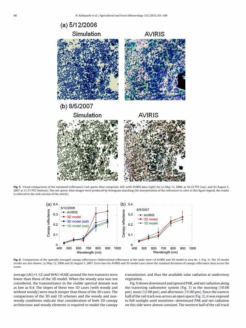
90 H. Kobayashi et al. / Agricultural and Forest Meteorology 152 (2012) 83– 100
Fig. 5. Visual comparisons of the simulated reflectance (red–green–blue composite, left) with AVIRIS data (right) for (a) May 12, 2006, at 10:22 PST (top), and (b) August 5,2007 at 11:57 PST (bottom). The red–green–blue images were produced by histogram matching (for interpretation of the references to color in this figure legend, the readeris referred to the web version of the article).
F flectanr IS ands
alcawcwa
ig. 6. Comparisons of the spatially averaged canopy reflectances (bidirectional reesults are also shown. (a) May 12, 2006 and (b) August 5, 2007. Error bars for AVIRcene.
verage LAI (=1.12) and WAI (=0.68) around the two transects wereower than those of the 3D model. When the woody area was notonsidered, the transmittance in the visible spectral domain wass low as 0.4. The slopes of these two 1D cases (with woody and
ithout woody) were much steeper than those of the 3D cases. Theomparisons of the 3D and 1D schemes and the woody and non-oody conditions indicate that consideration of both 3D canopy
rchitecture and woody elements is required to model the canopy
ce at the nadir view) of AVIRIS and 3D model in area No. 1 (Fig. 3). The 1D model 3D model cases show the standard deviation of canopy reflectance data across the
transmission, and thus the available solar radiation at understoryvegetation.
Fig. 9 shows downward and upward PAR, and net radiation alongthe traversing radiometer system (Fig. 3) in the morning (10:00
pm), noon (12:00 pm), and afternoon (15:00 pm). Since the easternhalf of the rail track was across an open space (Fig. 3), it was exposedto full sunlight until noontime—downward PAR and net radiationon this side were almost constant. The western half of the rail track
H. Kobayashi et al. / Agricultural and Forest Meteorology 152 (2012) 83– 100 91
Fig. 7. Comparisons of the spatially averaged reflectances for (a) the crowns and (b) the understory parts in area No. 1. The simulated results are from the 3D scheme. Errorbars show the standard deviation of bidirectional reflectance data across the scene.
Table 3Statistics of the comparison between the simulated (3D scheme) and measureddownward PAR, upward PAR, and net radiation (Rn) at the understory level alongthe rail track.
Slope Intercept r2 RMSE Bias
Downward PAR 0.99 68.25 0.97 136.79 65.93Outgoing PAR 0.70 12.18 0.90 29.66 −15.87Rn 0.88 15.25 0.95 56.95 −14.14
Positive biases indicate that the simulated results are higher than the measurements.RMSE: root mean square error. The RMSE and bias unit for downward and outgoingP
wiattnAir
datuddtaa1whn(ftcabtdocoFst
Fig. 8. Comparisons of the simulated canopy spectral transmittance (450 nm,550 nm, 650 nm, 780 nm, and 900 nm) averaged over the transect A (T-A) and C (T-C),blue: 3D model with woody elements. Red: 3D model without woody elements, andgreen: 1D model with and without woody elements. For 1D simulation, we used an
of track measurements in a same solar geometry, but they reduce
AR are �mol m−2 s−1, and for Rn are W m−2.
as located under the tree canopy. Therefore, the transect variabil-ty of downward PAR was associated with the sunlit and shadedreas that were formed as a geometric relationship between theree crowns and the sun direction. Until noon, the model capturedhe radiation variability along the rail track. However, in the after-oon, our model did not capture the variability along the rail track.lthough upward PAR was low due to the low ground reflectance
n the PAR region (Table 2), the variability in upward PAR along theail track was similar to those of downward PAR (Fig. 10).
Fig. 10 shows diurnal patterns of simulated and measuredownward and upward PAR, and Rn. The data shown here areveraged values along the rail track. Table 3 shows statistics ofhe comparison between simulated and measured radiation val-es. The simulated results capture the general diurnal patterns ofownward and upward PAR and Rn. There are two reasons for theifferences between the measured and simulated radiation. First,he differences in crown sizes and positions between modeled andctual trees around the rail track resulted in different downwardnd upward flux densities of PAR and Rn. For example on DOY94 15:00 pm (Fig. 9c), the peaks of the simulated PAR and Rn
ere found at about 10 m on the rail track. These peaks shouldave been aligned with the measured peaks at 12 m. In the after-oon, the sunlight comes from the west, where the track is shadedFig. 3), and the crowns cast elongated shadows eastward. There-ore, the spatial variation in downward PAR and Rn along the railrack was formed by smaller scale gaps between and inside therowns, which are more sensitive to the individual crown shapesnd lengths. The assumption of the spheroid crown shape with tur-id volumes blurred when simulating the small-scale variability ofhe solar radiation at the understory. The second reason for theifferences is the spatial variation in LAD and WAD in the crownbject. Our model assumed that LAD and WAD were constant in therown volumes. However, because of the actual spatial variabilityf LAD and WAD in the crowns, gap fractions did not match exactly.
or example, the simulated LAD, which can fit well with the mea-urements, depends on the position of the transects (Fig. 4). Forhe simplicity of the modeled trees, we assumed that there was aaverage LAI and WAI around the transect A and C (LAI = 1.12, WAI = 0.68) (for inter-pretation of the references to color in this figure legend, the reader is referred to theweb version of the article).
constant LAD and WAD inside the crown objects. That could causedifferences of PAR and Rn at the understory level.
Transect-based measurements along the rail track have anadvantage in that they produce spatially representative radiationenvironments. In particular, measurements from transects placedperpendicular to the sun direction maximize the spatial repre-sentation (Widlowski, 2010). Our rail track was placed along theeast-west direction; it gave the maximum variety of radiation spa-tially as the beam lights came from a southerly direction aroundnoontime. There was, however, a limitation on the length of therail track (20 m). For example, to evaluate the radiation environ-ment over the coverage of the eddy covariance footprint, we neededto deploy at least more than a 100 m transect. Such long transectmeasurements require faster velocity of the tram to keep the suite
the frequency of spatial samplings for the net radiometer as netradiometers have slower response (∼30 s) to the subtle changes inradiation environments.

92 H. Kobayashi et al. / Agricultural and Fore
Table 4Statistics of the 3D model results of net radiation (Rn), sensible heat (H), latent hear(�E), the ground heat (G), tree photosynthesis (Ps), and PAR albedo.
Slope Intercept R2 RMSE Bias
Rn 1.06 31.70 0.99 52.00 40.38H 1.20 −14.83 0.98 41.90 2.71�E 1.53 5.26 0.96 40.60 23.05G (soil) 1.46 −2.28 0.93 13.44 0.75Ps (Tree only) 1.02 0.04 0.95 0.79 0.08Albedo (PAR) 0.69 0.00 0.89 0.02 −0.01
Positive biases indicate that the simulated results are higher than the measurements.RMSE: root mean square error. The unit of RMSE and bias for Rn, H, �E, G are W m−2,and for Ps are �mol m−2 s−1, and for PAR albedo are unitless.
Fig. 9. Comparisons of the simulated and measured downward and upward PAR (PAR dowsystem at the woodland floor (DOY=194, 2008). (a) 10:00 am, (b) 12:00 pm, (c)15:00 pm.
Fig. 10. The comparisons of simulated and measured diurnal patterns of downward PARabove the ground along the rail track). The PAR down, PAR up and Rn are averaged valuetrack. Gaps on days 124 and 130 are due to missing data. (a) DOY 124 (b) DOY 130 (c) DO
st Meteorology 152 (2012) 83– 100
4.3. Energy flux densities and canopy photosynthesis
Figs. 11 and 12 and Table 4 show the comparisons between thesimulated (both 3D and 1D schemes) and measured energy fluxdensities (Rn, H, �E, and G) in four different periods. In the 1Dscheme, we did not include the woody elements because most ofthe 1D land surface models do not consider the sensible heat andheat storage of the woody elements. The comparison covers threedistinct seasons, (1) leafless crowns with green grass (DOY 68-74),
(2) fully foliated crowns and green grass (DOY 115-121) and (3)fully foliated crowns and dead grass with water deficits (DOY 188-194, 204-210). The simulated and measured Rn generally exhibitedthe similar seasonal and diurnal patterns. However, the peak Rnn and PAR up), and net radiation (Rn) along the transect of the traversing radiometer The x axis is a distance from the west edge of the track.
(PAR down), upward PAR (PAR up), and net radiation (Rn) at understory level (1 ms over the rail track transect, and error bars are standard deviations along the railY 194 (d) DOY 215.

H. Kobayashi et al. / Agricultural and Forest Meteorology 152 (2012) 83– 100 93
Fig. 11. Diurnal patterns of simulated (red line: 3D scheme, blue line: 1D scheme) and measured (dots) net radiation (Rn), sensible heat (H), and latent heat flux (�E) densities.F y grasa l wasd referr
smDu(
F1
our different periods in 2008 (DOY 68-75: non-foliated trees with active understornd 204-210: fully foliated trees with dead understory grasses) are shown. The modeata (for interpretation of the references to color in this figure legend, the reader is
imulated by the 3D model was 4%–11% higher than the measure-
ents, while the peak Rn by the 1D model agreed well except theOY 68-74 (8% error). The RMS errors show that H, �E, and G sim-lated by the 3D scheme were better than those of the 1D schemeFig. 12). In the 1D scheme, the large differences were found in DOYig. 12. Comparison of measured and simulated (3D and 1D) energy fluxes in four differe21: fully foliated trees with active understory grasses, DOY 188-194 and 204-210: fully
ses, DOY115-121: fully foliated trees with active understory grasses, DOY 188-194 run in area No. 2, and measurements are seven-day averages of the eddy covarianceed to the web version of the article).
68-74 and DOY 115-121 when the weather is mild and the soil is
wetter (Table 1); Sensible heat flux densities simulated by the 1Dscheme tend to be lower in those periods, and latent heat flux den-sities tend to be higher than the measurements. In the 1D scheme,the understory grass and the soil surface received more radiationnt periods (DOY 68-75: non-foliated trees with active understory grasses, DOY115-foliated trees with dead understory grasses).

94 H. Kobayashi et al. / Agricultural and Forest Meteorology 152 (2012) 83– 100
Fig. 13. Diurnal patterns of fraction of absorbed PAR (FAPAR) and NIR (FANIR) by tree leaves, understory grasses and woody elements in four different periods ((a) DOY68-75: non-foliated trees with active understory grasses, (b) DOY115-121: fully foliated trees with active understory grasses, (c) DOY 188-194 and (d) 204-210: fully foliatedtrees with dead understory grasses).
Fig. 14. Upper figures: diurnal patterns of simulated (lines) and measured (dots) tree canopy photosynthesis (Ps). Three different periods in 2008 (DOY 68-75: non-foliatedtrees with active understory grasses, DOY115-121: fully foliated trees with active understory grasses, DOY 188-194 and 204-210: fully foliated trees with dead understorygrasses) are shown. Lower figures: the diurnal course of air temperature (Tair) and vapor pressure deficit (VPD). The model was run in area No. 2, and measurements areseven-day averages of the eddy covariance data. Photosynthesis of understory grasses is not included in Ps.

d Forest Meteorology 152 (2012) 83– 100 95
tmohaesIs
ismdacr
(pcot0tTncacputbteasl
aet(Tiha(f2d2is
4h
uatifa
Fig. 15. Comparison of measured and simulated (3D and 1D) tree canopy photo-
H. Kobayashi et al. / Agricultural an
han those of the 3D scheme because of the lack of the woody ele-ents over the understory. For example, in DOY 68-74, the fraction
f absorbed PAR (FAPAR) simulated by the 1D scheme was 24%–42%igher than that of the 3D scheme. This caused an overestimation ofbsorbed radiation in understory grass and soil. Consequently, thisffect led to overestimation of the latent heat fluxes of grass andoil. In DOY 115-121, tree leaves and understory grass co-existed.n this period, FAPAR of the 1D scheme is higher than that of the 3Dcheme, and this caused overestimation of latent heat flux.
On the contrary, the differences between 3D and 1D schemesn the dry periods (DOY 188-194 and 204-210) were smaller. Theimulated results from both schemes agreed fairly well with theeasurements even though FAPAR from both scheme had some
ifferences (Fig. 13). In such periods, due to limited soil watervailability, the soil evaporation was negligibly small and the treeslosed most of their stomata, inhibiting the transpiration. As aesult, most of the absorbed energy was used as sensible heat.
The simulated energy fluxes by the 3D scheme closedH + �E)/(Rn − G − Swoody) = 1. If we exclude the woody storage com-onents, the simulated daytime and nighttime energy balancelosure (H + �E)/(Rn − G) were 0.88 and 0.77, respectively. On thether hand, the daytime and nighttime energy balance closure ofhe eddy covariance measurements (H + �E)/(Rn − G) were 0.81 and.17, respectively. For the daytime case, the simulated results showhe woody storage term accounts for 0.12 (12%) of all energy fluxes.he consideration of the landscape scale woody storage term sig-ificantly improves the accuracy of the measured energy balancelosure (from 0.81 to 0.93). For nighttime case, due to low windnd larger flux footprint, the energy balance closure was signifi-antly lower than 1. The consideration of the woody storage termotentially improve the energy balance closure, however, the largencertainty of the measurements impedes evaluating evaluationhe role of the nighttime stem storage flux. Energy imbalance haseen one of the important issues and therefore has been inves-igated thoroughly (Wilson et al., 2002). For example, Lindrotht al. (2010) found the significance of including the woody stor-ge component in spruce/pine forests. Our study site also shows aubstantial contribution of woody storage due to a heterogeneousandscape and high proportion of woody area to total plant area.
Fig. 14 shows the diurnal patterns of the simulated (3Dnd 1D) and the measured tree canopy photosynthesis (Ps) (Mat al., 2007). For DOY 115-121, with the moderate air tempera-ures (10 ◦C–24 ◦C) and sufficient soil water available to the treesTable 1), Ps was the largest among the three compared periods.he Ps simulated by the 1D scheme was large than the 3D schemen the morning. This is because the FAPAR of the 1D scheme isigher than the 3D scheme (Fig. 14). Moreover, VPD and air temper-ture are milder in the morning and less stress than the afternoonFig. 14). Thus, the Ps in the morning is more sensitive to the dif-erence in FAPAR than that in the afternoon. On DOY 188-194 and04-210, due to the high temperature and VPD, Ps was stronglyown-regulated by these factors as well as by a low Vcmax (Ma et al.,011). The differences between the 3D and 1D scheme were small
n those periods. Overall, the 3D scheme (RMSE = 1.15) performedlight better than that of the 1D scheme (RMSE = 1.56) (Fig. 15).
.4. Spatial variations of radiation fluxes across the canopyeights
Since our study site is heterogeneous a mismatch of the sim-lated and measured radiation fluxes in Fig. 11 was likely. Wenalyzed how the heterogeneity of the landscape affected the spa-
ial variation of the radiation fluxes around the flux tower locationn area No. 2. Fig. 16 shows upward PAR, NIR, TIR, and Rn at three dif-erent heights (understory level = 1 m, just above the canopy = 12 m,nd the flux tower height = 23 m). As the sampling height increased,synthesis at three different periods (DOY115-121: fully foliated trees with activeunderstory grasses, DOY 188-194 and 204-210: fully foliated trees with dead under-story grasses).
spatial variations of radiation fluxes were rapidly reduced. Thestandard deviations of the radiation fluxes at the flux tower height(23 m) were 1.3–16.4 W m−2 and their coefficients of variationswere 6.8% for upward PAR, 4.2% for upward NIR, 2.8% for upwardTIR, and 2.1% for Rn. Therefore, the spatial variations in the radia-tion streams were small. The reason why the spatial variations weresmall is attributed to the angular contributions of the incomingradiation of the PAR and Rn sensors. The contribution of incom-ing radiation to the PAR and Rn sensors is proportional to cos �оintegrated over the sphere (or hemisphere) with a weight of sin �о(Jacobian), where �о is a view zenith angle. Based on this weight,only 12% of radiation energies could be attributed to field of view<20◦, which is about the radius of 8.4 m at the ground. While wefound a similar size of open space just below the flux tower location,that open space did not significantly affect the representativenessin measuring the landscape scale radiation fluxes.
4.5. Effect of woody elements on radiation absorption by canopy
In CANOAK-FLiES, we explicitly defined woody areas in thecrowns. We estimated the woody area density from the gap fractionmeasurements based on digital cover photography. Moreover, ourenergy flux simulation implies a significant amount of the woodyheat storage. Fig. 13 shows diurnal patterns of a fraction of theabsorbed PAR (FAPAR) and a fraction of the absorbed NIR (FANIR)in four simulated periods. These results exhibited general temporalpatterns found in previous research (Widlowski, 2010). Generally,absorptions by woody elements were lower than those of leaves,but they were not negligible. The FAPAR and FANIR of the woodyelements contributed 12%–39% and 20%–52% of the total FAPAR andFANIR, respectively (Fig. 13). Particularly, in the NIR domain, leaftransmittance was higher than that in the PAR domain (Table 2),resulting in the higher absorption in woody elements via a con-tribution of radiation transmitted through the leaves. Due to thenature of the woodland structure at our site, the higher propor-tion of woody area to leaf area (42%) (Ryu et al., 2010a), causeda higher absorption in woody elements. Our results support theradiative transfer study by Asner et al. (1998), which also shows alarge amount of PAR absorption in woody elements (10–40%).
4.6. Overall performance and uncertainties of the 3D approach
The spatially explicit 3D radiative transfer and energyexchange model, CANOAK-FLiES, was developed to simulate

96 H. Kobayashi et al. / Agricultural and Forest Meteorology 152 (2012) 83– 100
Fig. 16. Spatial variations of upward radiation fluxes (PAR, NIR, and TIR) and net radiation at three different heights (1 m: understory level, 12 m: above the canopy, 23 m:e rianced PM, Ds refer
scstpmeetr2pt3(rLHbahUuwcdsFsN
ddy covariance tower height). The size of area is 100 by100 m and the eddy covaeviations (STD) are also shown (unit: W m−2). Simulation was performed at 12:00tem (for interpretation of the references to color in this figure legend, the reader is
patial distribution of radiation environments and energy andarbon fluxes. Recent advancement in obtaining detail canopytructure and radiation data sets enabled us to develop and validatehis type of 3D model. We employed airborne-based LiDAR dataroposed and validated by Chen et al. (2006). While CANOAK-FLiESostly captured the spatial and temporal patterns of radiation
nvironments, the current airborne-LiDAR data has a limitation inxtracting a canopy structure finer than a 1–2 m scale. In that scale,he use of ground-based LiDAR data improves the description ofadiation environments (Hosoi and Omasa, 2007; Zande et al.,009). Our 3D approach relies on the accurate canopy structuralarameters derived from the airborne LiDAR data. Currently,he availability and uncertainty of such data limit extending theD approach to other ecosystems. For example, Disney et al.2010) investigated the expected accuracy of the canopy heightetrieval from the discrete-return LiDAR system and found that theiDAR-based approach tended to underestimate the canopy height.opkinson (2007) also showed that the canopy heights retrievedy the LiDAR were sensitive to the sampling strategy such as flyingltitude, laser pulse repetition frequency. The errors in the crowneights and diameters could change the landscape heterogeneity.nderestimation of such parameters causes smaller crown vol-mes and thus overestimation of leaf and woody area densities ase estimate these variables by matching the simulated gap fraction
onstructed by the 3D canopy with the gap fractions taken by theigital photography. Consequently, underestimation of the canopy
tructural parameters can cause severe clumping, and lower treeAPAR, �E, and Ps. In other words, the improvement of canopytructure observation makes the model performance better.onetheless, the 3D approach will be useful to fill the theoreticaltower is located at the center of the images. Spatial averages (Avg.) and standardOY115, 2008. The small blue dots on the TIR image at 1 m level are the position of
red to the web version of the article).
gap between 1D model and the real ecosystems. Therefore, theimprovement of the LiDAR algorithms will be important.
In most of the past studies, 3D models were evaluated bytransect variability or diurnal patterns of PAR transmittance mea-surements (Law et al., 2001; Sinoquet et al., 2001; Tournebize andSinoquet, 1995; Wang and Jarvis, 1990), but few modeling studieshave tested the spatial variations of net radiation in heterogeneouslandscapes. In this study, we evaluated not only PAR transmittance,but also NIR, and the net radiation at the understory and at thetop of the canopy. Reliable simulation of net radiation is neededwhen computing energy fluxes. Therefore, reliable radiative trans-fer simulation in the TIR domain is crucial, and the TIR radiation canbe simulated from leaf temperature variations that are computedby the energy exchange model. We completed the simulation bycoupling the radiative transfer model with the energy exchangemodel. Also, spectral reflectance (bidirectional reflectance) andspectral transmittance allowed us to evaluate the effect of scatter-ing on transmittance and reflectance. Since our 3D model resultsof canopy reflectance and transmittance agreed well, the absorp-tion (=1 − reflectance − transmittance) simulated by the 3D modelshould be reliable. Furthermore, we also simulated radiation fluxesat several different vertical levels, including the understory andthe top of the canopy. Even though the tower was located in anopen space, contribution of the radiation flux from the understorylevel was marginal, as the spatial radiation fluxes blurred with anincrease in the height.
The CANOAK-FLiES simulation in 3D and 1D modes enabled usto examine the effect of landscape heterogeneity on energy andcarbon fluxes through the change in the simulated canopy radia-tion environments. Overall, the 3D scheme worked better than the

d Fore
1rwaotlbipfiivecwp
tio�(mptleatsosbiwfFcvmalpecbcibt
eirtiTimobebfiw
H. Kobayashi et al. / Agricultural an
D scheme. The effect of landscape heterogeneity depends on theadiative quantities. The difference between 3D and 1D schemesas negligible in canopy reflectance, but substantial in canopy
bsorption (FAPAR) and transmittance. The impact of heterogeneityn these radiation quantities will also depend on the stand struc-ure such as canopy LAI and crown cover. Wherever such diverseandscape conditions, the 3D approach is expected to provideetter solutions. This fact encourages re-designing the model-data
ntercomparison study based on the different level of model com-lexities from 3D (close to the actual ecosystems) to 1D with aner time scale (hourly). While the existing intercomparison stud-
es are likely to extract where to give wrong water and carbon fluxesia statistical or tuning approaches (e.g. Ichii et al., 2010; Mahechat al., 2010, Morales et al., 2005; Schwalm et al., 2010), a hierarchi-al model comparison approach with process-based understandingould improve the model reliability avoiding flaws of physics andhysiology.
Regarding �E and Ps, the 3D scheme generally performed bet-er than the 1D scheme. Yet, our comparison study reveals that themportance of accounting for the 3D canopy structure changes withther meteorological and physiological conditions. The notableE and Ps differences were found in wet mild weather periodsFigs. 11 and 14) because relative contribution of radiation environ-
ent to those fluxes was dominant in such periods. These resultsartly agree with the study by Song et al. (2009) as they concludedhat the heterogeneous canopy yielded lower �E and Ps at theoblolly pine stand. In the dry periods, however, the �E and Ps differ-nces between 3D and 1D scheme were not clear. According to thenalysis by Chen et al. (2008), the differences of the canopy archi-ecture modeled under the dry seasons with low LAI did not give aubstantial difference in Ps simulation. Our results, the differencef the canopy architectures (3D or 1D) were not relevant to Ps in dryeason, also coincided their results since the Ps is mostly controlledy the water availability via a change in photosynthetic capac-
ty (Vcmax). These results indicate that the light-limited (wet mildeather) periods force more reliable treatment in radiative trans-
er simulation than the water-limited periods (dry hot weather).urther study is necessary to investigate how the difference of theanopy structural modeling affects the seasonal and interannualariations in energy and carbon fluxes. In that situation, the inter-ediate complexity approach could fill the gap between 3D and 1D
pproach. For example, Chen et al. (2008) constructed oak wood-and landscapes by box-shaped trees and used to simulate canopyhotosynthesis. While Ps difference among the models with differ-nt complexity was negligible in dry periods, their intermediateomplexity approach should also be tested in wet mild periodsecause our results suggest that the effect of canopy structure onanopy photosynthesis is large in wet mild periods. Applying thisntermediate complexity approach to the wed mild periods, com-ined with our 3D approach, will provide how well and efficientlyhe models simulate the water and carbon fluxes.
This study indicates that the appropriate consideration of woodylements in the heterogeneous landscape is crucial for partition-ng the radiation environments (transmittance, absorption, andeflectance). The absence of woody elements resulted in higherransmittances (Fig. 8). In the NIR domain, woody elements inhib-ted the enhancement of the scattering radiation to some extent.he absorption of woody elements was also significant (12%–39%n PAR and 20%–52% in NIR). Consequently, the effect of woody ele-
ents on the energy balance simulation was not negligible. Indeed,ur simulated results suggest that 12% of available energy shoulde used for heat storage in woody elements. On the other hand, the
ffect of woody elements on the canopy reflectance was marginalecause the crown cover was low (47%) and many photons thatrst hit the leaves were scattered. Given that the high portion of theoody area, the accurate estimate of the woody area density leadsst Meteorology 152 (2012) 83– 100 97
to the robustness of the estimates of the radiation environment andthe energy fluxes including the heat storage term. We estimatedwoody area density by matching the simulated and measured gapfractions. However our best estimate of woody area density lieson 25% error. In addition, the crown architecture we assumed isstill simpler than reality; there is no interdependence between thelocation of leaves and branches. In fact, leaves are clumped aroundthe woody elements like twigs and formed as a shoot. Our crownassumption may lead overestimate or underestimate to the woodylight absorption. The improvement of the airborne and groundLiDAR-based canopy architectural estimate and more realistic treemodeling will reduce these uncertainties.
Further studies are needed to add modules that have not beenincluded in our model. Soil water effects on photosynthesis andevaporation were prescribed; we used soil moisture and photo-synthetic capacity (Vcmax) measurements for computation of soilevaporation and photosynthesis. Radiative transfer processes werefully modeled in 3D space explicitly, but the turbulence scheme wasstill one-dimensional and assumed the concentration field was wellmixed in the horizontal. This assumption could cause an error forthe concentration field within the crown objects. However, in ourstudy site, this effect should not cause a major source of the error insimulating energy fluxes since, in our model, leaves are distributedon the outer side of the crown canopies (Fig. 1), where the concen-tration field are in between the open space and the inside crown.We assumed that the crowns were spheroid with the same leafarea density. We divided the radiation into three broad spectralbands (PAR, NIR, TIR). Exploring the optimized number of spectralbands improves the radiative properties. One of the advantagesof the Monte Carlo radiative transfer model is that the computa-tion time does not increase when we divide the spectral domaininto more than three spectral domains; the statistical accuracy ofradiation only depends on the total number of photons. Nonethe-less, improvement of the computation time is necessary when themodel is run over a yearly time scale. In this study, diffuse skyradiances were assumed to be isotropic. Realistic information ofangular variations in atmospheric diffuse radiation improves theaccuracy of energy fluxes and photosynthesis (Hutchison et al.,1980).
5. Conclusion
We coupled a 3D shortwave and longwave radiative transfermodel with an energy and carbon exchange model (CANOAK-FLiES). This type of detailed modeling and testing was achieved bycollecting spatial and temporal shortwave and longwave radiationdata sets as well as other plant physiology and energy flux data sets.In particular, the tree structural information from airborne-LiDARenabled us to make a direct comparison of the spatial radiationenvironments with measurements. We evaluated the simulatedradiation fields in several different spectral domains (PAR, NIR, netradiation, and finer spectral domains of AVIRIS spectra) includingspatial and temporal patterns at understory and top of the canopylevels. Accurate computation of the radiation environments assuresthe reliability of the computation of energy fluxes.
Our model mostly captured the spatial and temporal patternsof radiation environments larger than a 1–2 m spatial scale. At theunderstory level, our model was able to simulate the spatial andtemporal patterns in PAR and net radiation, including the distinctpatterns between the open and shaded areas. At the top of the flux
tower, in spite of a heterogeneous condition at our study site, thespatial variability of the net radiation was small. Vertical profiles ofradiation fluxes suggest that the spatial heterogeneity of radiationfield blurred rapidly as the sensor height increases.
9 d Fore
3ecTpPh
l(aeFcutt
mavrcas
A
FooSc
A
NAEEEE�GHIPR
RRRRRSTTTguw˝
8 H. Kobayashi et al. / Agricultural an
The comparison between 3D and 1D schemes revealed that theD scheme generally performed better than the 1D scheme. How-ver, the importance of accounting for the 3D canopy structurehanges with other meteorological and physiological conditions.he 3D approach is more important in wet mild (light-limited)eriods than dry (water-limited) periods. The significant �E ands differences were found in wet mild weather periods because ofigh radiation sensitivity to �E and Ps.
When LAI is low and the fraction of woody elements is highike our study site, explicit consideration of the woody elementsbranches and stems) is crucial for realistic computation of radi-tion environments and energy fluxes. The significance of woodylements depends on the radiative properties (canopy reflectances,APAR, spectral transmitted light at the understory level). A signifi-ant amount of radiation was absorbed in the woody elements andsed for heat storage. Consideration of woody elements improvedhe daytime energy balance closure and afforded an accurate par-itioning of energy fluxes.
Since CANOAK-FLiES has a spatially explicit 3D structure, theodel is useful for the spatial analysis of radiation environments
nd energy fluxes. The model can help us to understand the obser-ations of heterogeneous landscapes and to check the spatialepresentativeness and design of measurements. Improvements inomputational efficiency, especially for radiative transfer schemes,re necessary to run the model over a yearly time scale and largerpatial scale.
cknowledgments
The first author was financially supported by the Postdoctoralellowship for Research Abroad of Japan Society for the Promotionf Science. The project was supported by the Office of Science (BER)f the U.S. Department of Energy (DE-FG02-03ER63638 and DE-C0005130). We thank Joseph Verfaillie for providing constructiveomments.
ppendix A.
omenclature Surface area of a simulated landscape (m2)tir,tot Total thermal emission in a simulated landscape (W)tir,s Thermal incoming radiation from the sky (W)tir,c Thermal emission from trees (W)tir,g Thermal emission from ground (W)E Latent heat flux (W m−2)
Soil heat flux (W m−2) Sensible heat flux (W m−2)
tir Thermal incoming radiation from the sky (W m−2)E Thermal emission probability distribution functionabs Absorbed shortwave (PAR and NIR) plus incoming long-
wave radiation (W m−2)PAR Absorbed PAR (W m−2)PAR,beam Absorbed beam PAR (W m−2)PAR,diffuse Absorbed diffuse PAR (W m−2)NIR Absorbed NIR (W m−2)TIR Absorbed TIR (W m−2)woody Heat storage in woody elements (W m−2)l Leaf temperature (C)w Woody temperature (C)g Soil temperature (C)
L Leaf angle distributionLeaf area density (m2 m−3)Woody area density (m2 m−3)
s(�s,�s) Sun direction vector
st Meteorology 152 (2012) 83– 100
˝l(�l,�l) Leaf surface normal vector˝E(�E,�E) Direction vector of thermal emission�, ��, �� Random numberεg Emissivity of the soil surfaceεl Emissivity of leavesεw Emissivity of woody elements� Stephan–Boltzmann constant (=5.67 × 10⁻⁸) (W m−2 K−4)
Appendix B.
Determination of the position of photon emission and the direc-tion of photon emission.
The total emission energy of a landscape can be written by:
Etir,tot = Etir,s + Etir,c + Etir,g, (B-1)
where Etir (W) is an emission energy, and the subscripts of tot, s,c, g indicate the emission energies of the total, the sky, the trees(the leaves plus the woody elements), and the ground emissionenergies. Etir,s was calculated by:
Etir,s = ItirA, (B-2)
where Itir (W m−2) and A (m2) are incoming TIR energy and a hor-izontal area of the landscape, respectively. Itir was obtained eitherfrom observations or simulations of atmospheric radiative transfermodel. Similarly, the emission from the ground, Etir,g, was derivedby integrating the local emission (=�εgT4
g(r)) over the ground sur-face (S):
Etir,g = �εg
∫s
T4g (r)dS, (B-3)
where � (W m−2 K−4) is the Stephan–Boltzmann constant(=5.67 × 10⁻⁸). εg is an emissivity of the ground. We assumed aconstant emissivity of the ground (εg = 0.98) over the simulatedlandscape. On the ground, the surface temperature varies with loca-tion due to the difference in the radiation conditions; some areasare exposed to sunlight and others are shaded. Total emission fromthe ground was, therefore, calculated by integrating the emissionat each point (r) over the landscape. Regarding the emission fromtrees, Etir,t, the contribution from both leaf and woody surfaceswas considered. Et was derived by integrating the local emission(=�εlT4
l(r)u(r) + �εwT4w(r)w(r)):
Etir,t = 2�
∫v{εlT
4l (r)u(r) + εwT4
w(r)w(r)}dV, (B-4)
where εl and εw are emissivities of leaf and woody materials,respectively. We multiplied by 2 to obtain the total emission fromthe both adaxial and abaxial sides, as u and w are defined by oneside of the leaf and one side of the woody surface areas. Finally, theprobability distribution function, PE(r) was obtained by:
PE(r) = Etir(r)Etir,tot
, (B-5)
where Etir(r) is a local emission in the simulated landscape.The spatial distribution of photon emission needed to follow
PE(r). We determined emission positions by two steps. First, wedetermined an emission category such as emission from the sky,trees, or ground, and then we determined an emission position.
The emission category was determined by a uniform random
number, � = [0,1], and the following criteria:0 < <
∫sky
PE(r)dS (B-6a)

d Fore
f∫
f∫
f
dwprp
˛
wgItr
tatbrs
�
f
�
f
�
somwFstv
˛
wndt
wEAwsmn
H. Kobayashi et al. / Agricultural an
or sky
sky
PE(r)dS < <
∫sky
PE(r)dS +∫
trees
PE(r)dV (B-6b)
or trees and understory grasses
sky
PE(r)dS +∫
trees
PE(r)dV < < 1 (B-6c)
or ground.Once the emission category was determined, a possible candi-
ate of the emission position, r = (x, y, z), in the selected categoryas determined using random numbers. To obtain the emissionosition that followed an emission energy distribution, we used aejection technique (Press et al., 1992). The criterion to select theosition was:
<Etir,i(r)Etir,i max
, (B-7)
here i is the subscripts s, t, or g, depending on the selected cate-ory. Etir,imax is maximum emission energy in the selected category.f the equation (B-7) meets a given �, the position was selected. Ifhe equation (B-7) did not meet a given �, the selected position wasejected and a new position was determined by random numbers.
The directions of emission ˝E(�E, �E) were determined to followhe angular distribution of emission of trees and the soil elementss well as by the incoming radiation from the sky. We assumed thathe emissions from the sky and the ground surface followed Lam-ert’s cosine law. Directions of emission from the soil and incomingadiation from the sky were calculated by the same equation as thecattering case, using two random numbers (��, ��):
E = 12
arccos(1 − 2˛�) (B-8a)
or sky
E = 12
{ + arccos(1 − 2˛�)} (B-8b)
or ground
E = 2�˛� . (B-8c)
On the leaf and woody surfaces, we also assumed that the emis-ions follow Lambert’s cosine law relative to the normal directionf leaf and woody surface. Therefore, the emission had to be deter-ined relative to given normal vectors ˝L(�L, �L) of the leaves andoody materials. We determined emission vectors by two steps.
irst, normal vectors of leaves and woody elements were randomlyelected using two random numbers. Then we applied the rejectionechnique to the selection or rejection of randomly selected normalectors. In �E direction, the following criterion was applied:
< gL(�L(˛�)), (B-9)
here gL is a leaf or woody angle distribution and �� is a randomumber. Azimuth direction �L was automatically selected when �Lirection was determined as we assumed the random distributiono the azimuth direction.
In the second step, the direction of emission relative to leaf oroody normal was determined using the same equations (B-8a–c).
mission occurs both from the surface of adaxial and abaxial sides.ssuming that the temperatures of the adaxial and abaxial sides
ere identical, either the adaxial or the abaxial side was randomlyelected. Finally, ˝E(�E, �E) was obtained by a coordinate transfor-ation from the emission direction relative to the leaf or woody
ormal.
st Meteorology 152 (2012) 83– 100 99
References
Antyufeev, V.S., Marshak, A.L., 1990. Monte-Carlo method and transport-equationin plant canopies. Remote Sensing of Environment 31 (3), 183–191.
Asner, G.P., Wessman, C.A., Archer, S., 1998. Scale dependence of absorption ofphotosynthetically active radiation in terrestrial ecosystems. Ecological Appli-cations 8 (4), 1003–1021.
Baldocchi, D., 1994. An analytical solution for coupled leaf photosynthesis and sto-matal conductance models. Tree Physiology 14 (7–9), 1069–1079.
Baldocchi, D., 1997. Measuring and modelling carbon dioxide and water vapourexchange over a temperate broad-leaved forest during the 1995 summerdrought. Plant Cell and Environment 20 (9), 1108–1122.
Baldocchi, D.D, Harley, P.C., 1995. Scaling carbon-dioxide and water-vapor exchangefrom leaf to canopy in a deciduous forest. 2. Model testing and application. PlantCell and Environment 18 (10), 1157–1173.
Baldocchi, D., Meyers, T., 1998. On using eco-physiological, micrometeorologicaland biogeochemical theory to evaluate carbon dioxide, water vapor and tracegas fluxes over vegetation: a perspective. Agricultural and Forest Meteorology90 (1–2), 1–25.
Baldocchi, D.D., Wilson, K.B., 2001. Modeling CO2 and water vapor exchange of atemperate broadleaved forest across hourly to decadal time scales. EcologicalModelling 142 (1–2), 155–184.
Baldocchi, D.D., Xu, L.K., Kiang, N., 2004. How plant functional-type, weather, sea-sonal drought, and soil physical properties alter water and energy fluxes of anoak-grass savanna and an annual grassland. Agricultural and Forest Meteorology123 (1–2), 13–39.
Ball, J.T., 1988. An Analysis of Stomata1 Conductance. Stanford University, CA, USA,89 pp.
Brutsaert, W., 1975. Derivable formula for long-wave radiation from clear skies.Water Resources Research 11 (5), 742–744.
Campbell, G., 1985. Soil Physics with Basic. Transport Models for Soil–Plant Systems150. Elsevier, Amsterdam.
Cescatti, A., 1997a. Modelling the radiative transfer in discontinuous canopies ofasymmetric crowns. I. Model structure and algorithms. Ecological Modelling100 (2/3), 263–274.
Cescatti, A., 1997b. Modelling the radiative transfer in discontinuous canopies ofasymmetric crowns. II. Model testing and application in a Norway spruce stand.Ecological Modelling 100 (2/3), 275–284.
Chen, Q., 2009. Improvement of the Edge-based Morphological (EM) methodfor lidar data filtering. International Journal of Remote Sensing 30 (4),1069–1074.
Chen, Q., Baldocchi, D., Gong, P., Kelly, M., 2006. Isolating individual trees in a savannawoodland using small footprint lidar data. Photogrammetric Engineering andRemote Sensing 72 (8), 923–932.
Chen, Q., Gong, P., Baldocchi, D., Tian, Y.Q., 2007a. Estimating basal area and stemvolume for individual trees from lidar data. Photogrammetric Engineering andRemote Sensing 73 (12), 1355–1365.
Chen, Q., Gong, P., Baldocchi, D., Xie, G., 2007b. Filtering airborne laser scanningdata with morphological methods. Photogrammetric Engineering and RemoteSensing 73 (2), 175–185.
Chen, Q., Baldocchi, D., Gong, P., Dawson, T., 2008. Modeling radiation andphotosynthesis of a heterogeneous savanna woodland landscape with a hier-archy of model complexities. Agricultural and Forest Meteorology 148 (6–7),1005–1020.
Disney, M.I., Kalogirou, V., Lewis, P., Prieto-Blanco, A., Hancock, S., Pfeifer, M., 2010.Simulating the impact of discrete-return lidar system and survey characteristicsover young conifer and broadleaf forests. Remote Sensing of Environment 114,1546–1560.
Gamon, J.A., Cheng, Y.F., Claudio, H., MacKinney, L., Sims, D.A., 2006. A mobile tramsystem for systematic sampling of ecosystem optical properties. Remote Sensingof Environment 103 (3), 246–254.
Gastellu-Etchegorry, J.P., 2008. 3D modeling of satellite spectral images, radiationbudget and energy budget of urban landscapes. Meteorology and AtmosphericPhysics 102 (3–4), 187–207.
Gutschick, V., 1990. Joining Leaf Photosynthesis Models and Canopy Photon-Transport Models. Springer-Verlag, Berlin.
Haverd, V., Cuntz, M., Leuning, R., Keith, H., 2007. Air and biomass heat storage fluxesin a forest canopy: calculation within a soil vegetation atmosphere transfermodel. Agricultural and Forest Meteorology 147 (3–4), 125–139.
Hopkinson, C., 2007. The influence of flying altitude, beam divergence, and pulserepetition frequency on lase pulse return intensity and canopy frequency dis-tribution. Canadian Journal of Remote Sensing 33 (4), 321–324.
Hosoi, F., Omasa, K., 2007. Factors contributing to accuracy in the estimation of thewoody canopy leaf area density profile using 3D portable lidar imaging. Journalof Experimental Botany 58 (12), 3463–3473.
Hutchinson, B.A., Matt, D.R., McMillen, R.T., 1980. Effects of sky brightness distribu-tion upon penetration of diffuse-radiation through canopy gaps in a deciduousforest. Agricultural Meteorology 22 (2), 137–147.
Ichii, K., Suzuki, T., Kato, T., Ito, A., Hajima, T., Ueyama, M., Sasai, T., Hirata, R., Sai-gusa, N., Ohtani, Y., Takagi, K., 2010. Multi-model analysis of terrestrial carboncycles in Japan: limitations and implications of model calibration using eddy
flux observations. Biogeosciences 7 (7), 2061–2080.Kim, J., Guo, Q., Baldocchi, D.D., Leclerc, M.Y., Xu, L., Schmid, H.P., 2006. Upscalingfluxes from tower to landscape: overlaying flux footprints on high-resolution(IKONOS) images of vegetation cover. Agricultural and Forest Meteorology 136(3–4), 132–146.

1 d Fore
K
K
L
L
M
M
M
M
M
M
M
M
N
N
P
P
P
P
R
R
R
00 H. Kobayashi et al. / Agricultural an
obayashi, H., Iwabuchi, H., 2008. A coupled 1-D atmosphere and 3-D canopyradiative transfer model for canopy reflectance, light environment, and pho-tosynthesis simulation in a heterogeneous landscape. Remote Sensing ofEnvironment 112 (1), 173–185.
ucharik, C.J., Norman, J.M., Gower, S.T., 1998. Measurements of branch area andadjusting leaf area index indirect measurements. Agricultural and Forest Mete-orology 91 (1–2), 69–88.
aw, B.E., Cescatti, A., Baldocchi, D.D., 2001. Leaf area distribution and radiative trans-fer in open-canopy forests: implications for mass and energy exchange. TreePhysiology 21 (12–13), 777–787.
indroth, A., Molder, M., Lagergren, F., 2010. Heat storage in forest biomass improvesenergy balance closure. Biogeosciences 7 (1), 301–313.
a, S.Y., Baldocchi, D.D., Xu, L.K., Hehn, T., 2007. Inter-annual variability in car-bon dioxide exchange of an oak/grass savanna and open grassland in California.Agricultural and Forest Meteorology 147 (3–4), 157–171.
a, S., Baldocchi, D.D., Mambelli, S., Dawson, T.E., 2011. Are temporal variations ofleaf traits responsible for seasonal and inter-annual variability in ecosystem CO2
exchange? Functional Ecology 25 (1), 258–270.acfarlane, C., Hoffman, M., Eamus, D., Kerp, N., Higginson, S., McMurtrie,
R., Adams, M., 2007. Estimation of leaf area index in eucalypt forestusing digital photography. Agricultural and Forest Meteorology 143 (3–4),176–188.
ahecha, M.D., Reichstein, M., Jung, M., Seneviratne, S.I., Zaehle, S., Beer, C.,Braakhekke, M.C., Carvalhais, N., Lange, H., Le Maire, G., Moors, E., 2010. Com-paring observations and process based simulations of biosphere atmosphereexchanges on multiple timescales. Journal of Geophysical Research 115, G02003,doi:10.1029/2009JG001016.
alenovsky, Z., Martin, E., Homolová, L., Gastellu-Etchegorry, J.-P., Zurita-Milla, R.,Schaepman, M.E., Pokorny, R., Clevers, J.G.P.W., Cudlín, P., 2008. Influence ofwoody elements of a Norway spruce canopy on nadir reflectance simulated bythe DART model at very high spatial resolution. Remote Sensing of Environment112 (1), 1–18.
archuk, G., Mikhailov, G., Nazaraliev, M., Darbinjan, R., Kargin, B., Elepov, B., 1980.The Monte Carlo Methods in Atmospheric Optics. Springer-Verlag.
edlyn, B., 2004. A MAESTRO Retrospective. Forests at the Land-Atmosphere Inter-face. CABI Publishing.
orales, P., Sykes, M.T., Prentice, I.C., Smith, P., Smith, B., Bugmann, H., Zierl, B.R.,Friedlingstein, P., Viovy, N., Sabate, S., Sanchez, A., Pla, E., Gracia, C.A., Sitch, S.,Arneth, A., Ogee, J., 2005. Comparing and evaluating process-based ecosystemmodel predictions of carbon and water fluxes in major European forest biomes.Global Change Biology 11 (12), 2211–2233.
orman, J.M., Welles, J.M., 1983. Radiative-Transfer in an Array of Canopies. Agron-omy Journal 75 (3), 481–488.
orth, P.R.J., 1996. Three-dimensional forest light interaction model using a MonteCarlo method. IEEE Transactions on Geoscience and Remote Sensing 34 (4),946–956.
aw, U.K.T., 1987. Mathematical-analysis of the operative temperature and energybudget. Journal of Thermal Biology 12 (3), 227–233.
inty, B., Gobron, N., Widlowski, J.-L., Gerstl, S.A.W., Verstraete, M.M., Antunes, M.,Bacour, C., Gascon, F., Gastellu, J.-P., Goel, N., Jacquemoud, S., North, P., Qin, W.,Thompson, R., 2001. Radiation transfer model intercomparison (RAMI) exercise.Journal of Geophysical Research-Atmospheres 106 (D11), 11937–11956.
inty, B., Widlowski, J.-L., Taberner, M., Gobron, N., Verstraete, M.M., Disney, M.,Gascon, F., Gastellu, J.-P., Jiang, L., Kuusk, A., Lewis, P., Li, X., Ni-Meister, W., Nil-son, T., North, P., Qin, W., Su, L., Tang, S., Thompson, R., Verhoef, W., Wang,H., Wang, J., Yan, G., Zang, H., 2004. Radiation Transfer Model Intercompar-ison (RAMI) exercise: results from the second phase. Journal of GeophysicalResearch-Atmospheres 109 (D6), 19.
ress, W.H., Teukolsky, S.A., Vetterling, W.T., Flannery, B.P., 1992. Numerical Recipesin Fortran 77: the Art of Scientific Computing, second ed. Cambridge UniversityPress, Cambridge, 933 pp.
aupach, 1989. Applying Lagrangian fluid mechanics to infer scaler source distri-butions from concentration profiles in plant canopies. Agricultural and ForestMeteorology 47, 85–108.
yu, Y., Sonnentag, O., Nilson, T., Vargas, R., Kobayashi, H., Wenk, R., Baldocchi, D.D.,
2010a. How to quantify tree leaf area index in an open savanna ecosystem: amulti-instrument and multi-model approach. Agricultural and Forest Meteorol-ogy 150 (1), 63–76.yu, Y., Nilson, T., Kobayashi, H., Sonnentag, O., Law, B.E., Baldocchi, D.D.,2010b. On the correct estimation of effective leaf area index: does it reveal
st Meteorology 152 (2012) 83– 100
information on clumping effects? Agricultural and Forest Meteorology 150,463–472.
Sankaran, M., Hanan, N.P., Scholes, R.J., Ratnam, J., Augustine, D.J., Cade, B.S., Gignoux,J., Higgins, S.I., Roux, X.L., Ludwig, F., Ardo, J., Banyikwa, F., Bronn, A., Bucini, G.,Caylor, K.K., Coughenour, M.B., Diouf, A., Ekaya, W., Feral, C.J., February, E.C.,Frost, P.G.H., Hiernaux, P., Hrabar, H., Metzger, K.L., Prins, H.H.T., Ringrose, S.,Sea, W., Tews, J., Worden, J., Zambatis, N., 2005. Determinants of woody coverin African savannas. Nature 438 (7069), 846–849.
Scholes, R.J., Archer, S.R., 1997. Tree–grass interactions in savannas. Annual Reviewof Ecology and Systematics 28, 517–544.
Schwalm, C.R., Williams, C.A., Schaefer, K., Anderson, R., Arain, M.A., Baker, I., Barr, A.,Black, T.A., Chen, G., Chen, J.M., Ciais, P., Davis, K.J., Desai, A., Dietze, M., Dragoni,D., Fischer, M.L., Flanagan, L.B., Grant, R., Gu, L., Hollinger, D., Izaurralde, R.C.,Kucharik, C., Lafleur, P., Law, B.E., Li, L., Li, Z., Liu, S., Lokupitiya, E., Luo, Y., Ma, S.,Margolis, H., Matamala, R., McCaughey, H., Monson, R.K., Oechel, W.C., Peng, C.,Poulter, B., Price, D.T., Riciutto, D.M., Riley, W., Sahoo, A.K., Sprintsin, M., Sun, J.,Tian, H., Tonitto, C., Verbeeck, H., Verma, S.B., 2010. A model data intercompar-ison of CO2 exchange across North America: results from the North AmericanCarbon Program site synthesis. Journal of Geophysical Research 115, G00H05,doi:10.1029/2009JG001229.
Silberstein, R.P., Sivapalan, M., Viney, N.R., Held, A., Hatton, T.J., 2003. Modelling theenergy balance of a natural jarrah (Eucalyptus marginata) forest. Agricultural andForest Meteorology 115 (3–4), 201–230.
Sinoquet, H., Bonhomme, R., 1992. Modeling radiative-transfer in mixed and rowintercropping systems. Agricultural and Forest Meteorology 62 (3–4), 219–240.
Sinoquet, H., Le Roux, X., Adam, B., Ameglio, T., Daudet, F.A., 2001. RATP: a modelfor simulating the spatial distribution of radiation absorption, transpiration andphotosynthesis within canopies: application to an isolated tree crown. Plant Celland Environment 24 (4), 395–406.
Song, C., Katul, G., Oren, R., Band, L.E., Tague, C.L., Stoy, P.C., McCarthy, H.R., 2009.Energy, water, and carbon fluxes in a loblolly pine stand: results from uni-form and gappy canopy models with comparisons to eddy flux data. Journalof Geophysical Research 114, G04021, doi:10.1029/2009JG000951.
Thomson, 1987. Criteria for the selection of stochastic models of particle trajectoriesin turbulent flows. Journal of Fluid Mechanics 180, 529–556.
Tournebize, R., Sinoquet, H., 1995. Light interception and partitioning in ashrub/grass mixture. Agricultural and Forest Meteorology 72 (3–4), 277–294.
Verrelst, J., Schaepman, M.E., Malenovsky, Z., Clevers, J., 2010. Effects of woodyelements on simulated canopy reflectance: implications for forest chlorophyllcontent retrieval. Remote Sensing of Environment 114 (3), 647–656.
Wang, Y.P., Jarvis, P.G., 1990. Description and validation of an array model—Maestro.Agricultural and Forest Meteorology 51 (3–4), 257–280.
Watanabe, T., Ohtani, Y., 1998. A comparative study on calculation methods of heatconduction in tree stems. Journal of Agricultural Meteorology 54 (1), 47–54.
Widlowski, J.-L., 2010. On the bias of instantaneous FAPAR estimates in open-canopyforests. Agricultural and Forest Meteorology 150, 1501–1522.
Widlowski, J.-L., Taberner, M., Pinty, B., Bruniquel-Pinel, V., Disney, M., Fernan-des, R., Gastellu-Etchegorry, J.-P., Gobron, N., Kuusk, A., Lavergne, T., Leblanc,S., Lewis, P.E., Martin, E., Mottus, M., North, P.R.J., Qin, W., Robustelli, M.,Rochdi, N., Ruiloba, R., Soler, C., Thompson, R., Verhoef, W., Verstraete, M.M.,Xie, D., 2007. Third Radiation Transfer Model Intercomparison (RAMI) exercise:documenting progress in canopy reflectance models. Journal of GeophysicalResearch-Atmospheres 112 (D9), 28.
Widlowski, J.-L., Pinty, B., Clerici, M., Dai, Y., De Kauwe, M., de Ridder, K., Kallel, A.,Kobayashi, H., Lavergne, T., Ni-Meister, W., Olchev, A., Quaife, T., Wang, S., Yang,W., Yang, Y., Yuan, H., 2011. RAMI4PILPS: an intercomparison of formulations forthe partitioning of solar radiation in land surface models. Journal of GeophysicalResearch 116, G02019, doi:10.1029/2010JG001511.
Wilson, K., Goldstein, A., Falge, E., Aubinet, M., Baldocchi, D., Berbigier, P., Bernhofer,C., Ceulemans, R., Dolman, H., Field, C., Grelle, A., Ibrom, A., Law, B.E., Kowalski,A., Meyers, T., Moncrieff, J., Monson, R., Oechel, W., Tenhunen, J., Valentini, R.,Verma, S., 2002. Energy balance closure at FLUXNET sites. Agricultural and ForestMeteorology 113 (1–4), 223–243.
Xu, L.K, Baldocchi, D.D., 2003. Seasonal trends in photosynthetic parameters andstomatal conductance of blue oak (Quercus douglasii) under prolonged summer
drought and high temperature. Tree Physiology 23 (13), 865–877.Zande, D.V., Mereu, S., Nadezhdina, N., Cermak, J., Muys, B., Coppin, P., Manes, F.,2009. 3D upscaling of transpiration from leaf to tree using ground-based LiDAR:application on a Mediterranean Holm oak (Quercus ilex L.) tree. Agricultural andForest Meteorology 149 (10), 1573–1583.