Modeling complex geological structures with elementary training images and transform-invariant...

Modeling complex geological structures with elementary trainingimages and transform-invariant distances

Gregoire Mariethoz1 and Bryce F. J. Kelly1

Received 14 January 2011; revised 21 April 2011; accepted 20 May 2011; published 14 July 2011.

[1] We present a new framework for multiple-point simulation involving small andsimple training images. The use of transform-invariant distances (by applying randomtransformations) expands the range of structures available in the simple patterns of thetraining image. The training image is no longer regarded as a global conceptual geologicalmodel, but rather a basic structural element of the subsurface. Complex geologicalstructures are obtained whose spatial structure can be parameterized by adjusting thestatistics of the random transformations, on the basis of field data or geological context. Inmost cases, such parameterization is possible by adjusting two numbers only. This methodallows us to build models that (1) reproduce shapes corresponding to a desired priorgeological concept and (2) are in phase with different types of field observations such asorientation, hydrofacies, or geophysical measurements. The main advantage is that thetraining images are so simple that they can be easily built even in 3-D. We apply the methodon a synthetic example involving seismic data where the transformation parameters aredata-driven. We also show examples where realistic 2- and 3-D structures are built fromsimplistic training images, with transformation parameters inferred using a small number oforientation data.

Citation: Mariethoz, G., and B. F. J. Kelly (2011), Modeling complex geological structures with elementary training images and

transform-invariant distances, Water Resour. Res., 47, W07527, doi:10.1029/2011WR010412.

1. Introduction[2] Numerical subsurface models often rely on scarce

data that are insufficient for determining the nature of the ge-ological continuity at a given site. Hence, in most situationsthe geologist’s contextual insights are a crucial source ofprior information. In the Earth sciences, a prior model repre-sents this knowledge, i.e., what is known of the geologicalcontinuity before the inclusion of location-dependent data.In general, the fewer local data available, the greater the im-portance of the prior model. Prior spatial continuity can becharacterized in various ways. Figure 1 illustrates variousprior concepts of geological continuity that can have verydifferent implications in terms of flow and transport proper-ties. They could, for example, correspond to: (1) folded par-allel structures of alternating high and low permeabilityvalues (Figure 1a and 1b); (2) high permeability values wellconnected together and defining boundaries between discon-nected blocks of low values (Figure 1c and 1d); (3) lowpermeability values well connected together and definingboundaries between disconnected blocks of high values(Figure 1e); and (4) connectivity of high values and connec-tivity of low values, spatially arranged as elongated bodies(Figure 1f).

[3] Existing geostatistical simulation methods are ableto represent such priors. However, at present only multi-Gaussian models offer the possibility to easily define thespatial structure with only a few parameters (mean, variance,and correlation length). Therefore, the multi-Gaussian frame-work offers possibilities for including such parameters inoptimization frameworks [Kitanidis, 1995; Nowak et al.,2010], e.g., finding the variogram parameters that are coher-ent with state data such as groundwater head or concentra-tion measurements.

[4] Within the multi-Gaussian framework, a wealth oftechniques exist to generate diverse shapes by combiningdifferent Gaussian random fields, such as the plurigaussianmethod [Le Loc’h and Galli, 1994; Mariethoz et al., 2009]or the random coordinate perturbation method and the ran-dom mixture of Gaussian fields [Emery, 2007]. Thesemethods have the advantage of allowing for parameteriza-tion of the prior through the definition of correlation ranges,cutoffs, etc. A parametric spatial model is of interest formodel inference and inverse modeling. In certain cases,however, the assumptions underlying these multi-Gaussianmodels do not allow for the reproduction of the behavior ofhighly heterogeneous aquifers, especially when connectiv-ity patterns play an important role [Bastante et al., 2008;Gomez-Hernandez and Wen, 1998; Knudby and Carrera,2005; Sanchez-Vila et al., 1996; Western et al., 2001].This can have an especially strong impact when modelingtransport processes [Green et al., 2010; Klise et al., 2009;Zinn and Harvey, 2003]. Therefore, several alternative sim-ulation methods have been developed in the past decades.One approach is to use parametric mathematical models,

1National Centre for Groundwater Research and Training, University ofNew South Wales, Sydney, New South Wales, Australia.

Copyright 2011 by the American Geophysical Union.0043-1397/11/2011WR010412

W07527 1 of 14

WATER RESOURCES RESEARCH, VOL. 47, W07527, doi:10.1029/2011WR010412, 2011

but to enrich the statistical information by including high-order measures of spatial continuity. Among this promisingclass of methods spatial cumulants [Dimitrakopoulos et al.,2010] and copulas [Bardossy and Li, 2008] have recentlyreceived a lot of attention.

[5] Other approaches such as object-based [e.g., Deutschand Wang, 1996; Deutsch and Tran, 2002; Keogh et al.,2007; Pyrcz et al., 2009] and pseudo-genetic models[Cojan et al., 2004; Michael et al., 2010] have been tradi-tionally used to account for the existence of specific con-nectivity patterns. The main advantage is their ability todefine basic shapes that represent geological bodies, usingphysical representations of the primary geological proc-esses and settings. Conditioning to points data and to non-stationarity in the objects’ proportions can be accomplished

through a birth and death algorithm [Allard et al., 2006;Lantuejoul, 2002], but technical and computational difficul-ties remain when large amounts of data are present. One ofthe advantages of the Boolean framework is that the charac-teristics of the objects used in the simulation can be adjustedto a certain extent (e.g., channel width, sinuosity, etc.).

[6] Recent advances in the domain of geostatistical sim-ulations include multiple-point simulation methods (MPS),which use prior spatial models given by nonparametricconceptual example images, namely training images. Theprinciple of a training image is appealing to geologistsbecause it is a direct representation of a geological concept[Feyen and Caers, 2006]. It has been shown that MPS areable to produce geologically realistic structures by usinghigh-order spatial statistics, which can represent a wide

Figure 1. Different prior concepts of geological continuity. (a) Slump folding in mudstone, WardenHead, New South Wales, Australia. (b) Kink folds in interbedded phyllite and quartz greywacke, Kelso-Sofala Road, New South Wales, Australia. (c) Jointed granite, Sierra Mountain, California, UnitedStates. (d) Desiccation cracks in Vertosol soil, Narrabri, New South Wales, Australia. (e) HawkesburySandstone thin section. (f) Braided river channels, Diamantina River, Queensland, Australia (image Goo-gle Earth, Cnes/Spot, Whereis Sensis, DigitalGlobe). (Figures 1a–1c and Figure 1e courtesy of BryceKelly. Figure 1d courtesy of Anna Greve.)

W07527 MARIETHOZ AND KELLY: MPS WITH ELEMENTARY TRAINING IMAGES W07527

2 of 14

range of spatially structured, low entropy phenomena, andhave been used in a variety of cases [e.g., Caers, 2003;Gonzales et al., 2008; Hu and Chugunova, 2008; Huys-mans and Dassargues, 2009; Journel and Zhang, 2006; Luet al., 2009; Okabe and Blunt, 2007; Ronayne et al., 2008;Wojcik et al., 2009; Wu et al., 2008].

[7] However, although MPS has in recent years becomean invaluable tool to integrate geological concepts in sub-surface models, the method is still difficult to apply in caseswhen one does not have enough information to clearlydecide which training image to use [de Almeida, 2010;Pyrcz et al., 2008]. Even when the geological context isclear, it is a lengthy geomodeling exercise to build a com-plex 3-D training image that adequately represents the com-plexity of geological structures.

[8] Another difficulty is related to the parameterizationof the training image. Since the choice of a training imageis a discrete decision (either image A or B), it is notstraightforward to parameterize it. Suzuki and Caers [2008]proposed a methodology for investigating prior uncertaintyin the context of inverse problems through the use of dis-tances between a large variety of discrete scenarios. How-ever, it is still highly desirable to parameterize differentmultiple-point priors with only a few continuous parame-ters, in a similar way as multi-Gaussian priors. This is gen-erally not possible because the training images normallyused are too complex to be parameterized simply. Trainingimages are generally large (Strebelle [2002] recommendsuse of a training image much larger than the simulation do-main) and ideally contain enough diversity to encompassall possible patterns to be found in the simulation domain.

[9] Even if robust tools exist for multiple-point simula-tion, the practical difficulties related to building andparameterizing the training image often lead to discardingmultiple-point methods and to adopt parametric alterna-tives for the inferences of spatial continuity, such as tradi-tional variogram-based techniques. Nonetheless, there arecases where more prior information is available than a two-point model of spatial correlation. For example, on a givensite, one can often determine very general prior characteris-tics (e.g., connectivity or disconnectivity of the high val-ues), but the precise types of structures (orientation anddimensions of the structures) are usually uncertain. In thesecases, it is desirable to have methods that integrate suchprior characteristics in stochastic models while leavingunknown characteristics random.

[10] In this paper we present a new concept and algo-rithm for multiple-point simulation that considers elemen-tary/simplistic training images that are an expression ofprior spatial continuity. During the simulation the diversityof patterns is enriched by applying random transformations.It is equivalent to comparing patterns up to a transforma-tion, or using a transform-invariant distance. This methodenables the generation of complex geological imageswhose spatial structure can be parameterized by adjustingthe statistics of the random transformations. In most cases,such parameterization is possible by adjusting only twonumbers. It allows parameterizing multiple-point priors ina straightforward and integrated manner. Moreover, it alsoresolves the problem of building a training image becausebuilding elementary images is easy even in 3-D. The train-ing image is no longer regarded as a global conceptual

geological model, but rather a basic structural element ofthe subsurface, such as the shapes used in object-based sim-ulations. These basic elements can be parameterized to cre-ate models that (1) reproduce shapes corresponding to adesired prior geological concept, and (2) are in phase withdifferent types of field observations such as orientation,hydrofacies, or geophysical measurements.

[11] Section 2 of the paper is a short description of thedirect sampling method, which is the geostatistical simula-tion method used to illustrate our concept. Note, however,that the fundamental idea could, in theory and regardless ofimplementation issues, be applied to any simulation algo-rithm that is based on the computation of a distancebetween patterns. Section 3 details the concept of trans-form-invariant distances and elementary training images,and illustrates this concept with basic examples. Section 4shows how conditioning data can be used to structurallyguide the simulation. Finally, Section 5 shows how to intro-duce nonstationarity in the transformation parameters tomodel complex geological structures.

2. Background on the Direct Sampling Method[12] The direct sampling method is described in details

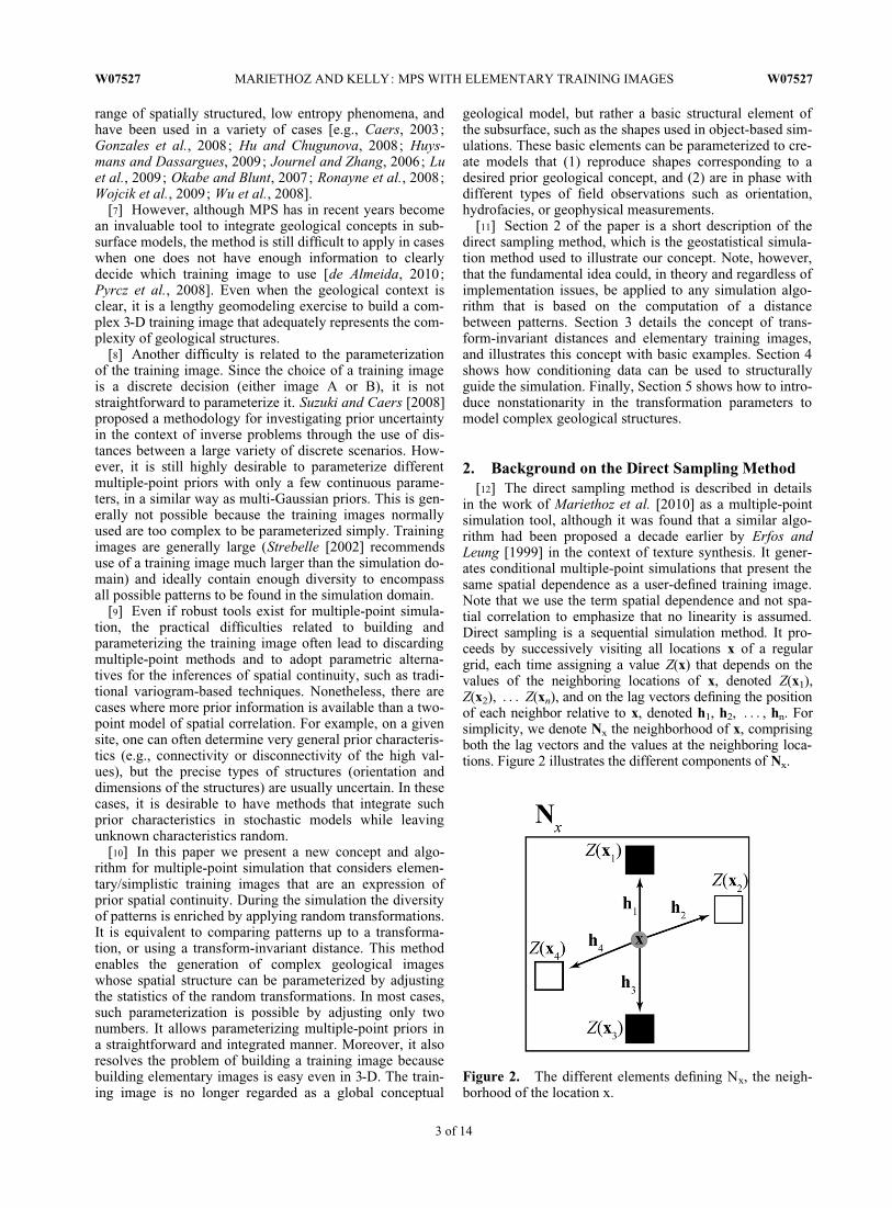
in the work of Mariethoz et al. [2010] as a multiple-pointsimulation tool, although it was found that a similar algo-rithm had been proposed a decade earlier by Erfos andLeung [1999] in the context of texture synthesis. It gener-ates conditional multiple-point simulations that present thesame spatial dependence as a user-defined training image.Note that we use the term spatial dependence and not spa-tial correlation to emphasize that no linearity is assumed.Direct sampling is a sequential simulation method. It pro-ceeds by successively visiting all locations x of a regulargrid, each time assigning a value Z(x) that depends on thevalues of the neighboring locations of x, denoted Z(x1),Z(x2), . . . Z(xn), and on the lag vectors defining the positionof each neighbor relative to x, denoted h1, h2, . . . , hn. Forsimplicity, we denote Nx the neighborhood of x, comprisingboth the lag vectors and the values at the neighboring loca-tions. Figure 2 illustrates the different components of Nx.

Figure 2. The different elements defining Nx, the neigh-borhood of the location x.


3 of 14

[13] The direct sampling algorithm is summarizedbelow:

Input: (1) Simulation grid SG with locations denoted x,(2) training image TI with locations denoted y, (3) distancefunction d(.) bounded in [0,1], (4) distance threshold t (dis-tance under which two neighborhoods are considered iden-tical).

1. While # noninformed locations in SG � 0 do.2. Choose a noninformed location x in SG and identify

the neighborhood Nx centered on x.3. Initialize dðNx;NyÞ ¼ 1.4. While dðNx;NyÞ � t do.5. Sample a location y in TI.6. Define Ny as the neighborhood centered on y having

identical lag vectors as Nx.7. Compute the distance dðNx;NyÞ.8. End While.9. Assign Z(x) ¼ Z(y).10. End While.Output: Completed simulation SG.The main principle is that as soon as a matching neigh-

borhood is found (i.e., when dðNx;NyÞ < t, one can con-sider that (Ny : Nx), the corresponding value Z(y) is asample of the conditional distribution Prob fZ(x)jNxg).

[14] The distance dðNx;NyÞ can be computed in differentways depending on the nature of the variable Z. It wasshown by Mariethoz et al. [2010] that choosing the appro-priate distance allows one to adapt the method to either cat-egorical or continuous variable cases, and also to jointlysimulate several dependant variables. The distances pro-posed include, for a categorical variable,

dðNx;NyÞ ¼1n

Xn

i¼1

ai 2 ½0; 1�;

where ai ¼0 if ZðxiÞ ¼ ZðyiÞ1 if ZðxiÞ 6¼ ZðyiÞ

(;

ð1Þ

and for a continuous variable, the normalized Manhattandistance

dðNx;NyÞ ¼1n

Xn

i¼1

ZðxiÞ � ZðyiÞj jmaxy2TI

ZðyÞ �miny2TI

ZðyÞ: ð2Þ

[15] Since the distances are usually defined such thatthey are within the interval [0,1], the threshold is alsobound to the same interval. Defining a threshold of t ¼ 0means that the patterns of the training image will be repro-duced with the highest possible accuracy. Conversely,when setting t ¼ 1, the algorithm unconditionally samplesvalues from the training image, therefore reproducing themarginal distribution of Z but with no spatial dependence.Between these two extreme cases, the value of t determineshow accurately the patterns of the training image arereproduced.

3. Transform-Invariant Distances3.1. The Principle of Transform-Invariant Distances

[16] Let us define a geometrical transformation Tp appliedto Nx, where p is a parameter affecting the transformation.

Several types of geometrical transformations can be consid-ered. For now, we consider two types of transformations,which are (1) rotations centered on x, denoted R(.), and (2)affinity (or homothetic) transforms, denoted A(.). Note thatwe consider only geometrical transforms that affect the lagvectors h while the values Z(xi) remain unchanged. For rota-tions, the parameter p corresponds to the rotation angle andfor affinity transforms, it corresponds to the affinity ratio.Figure 3 shows a few examples of transformations applied toa simple neighborhood (or pattern) Nx.

[17] The direct sampling method uses a distance betweena neighborhood Nx centered on the location x, and anotherneighborhood Ny centered on location y in the trainingimage (see step 7 of the algorithm). Instead, we propose aconsideration of the distance between the ensemble of pos-sible neighborhoods resulting from geometric transforms ofNx and a neighborhood Ny in the training image. By doingthis, we compare the neighborhoods Nx and Ny up to atransformation (i.e., there exists a transformation T(.) thatmakes T(Nx) identical to Ny). When considering transform-invariant distances, Figure 3a, 3b, and 3c are identical up toa rotation, and Figure 3a, 3d, and 3e are identical up to anaffinity. We define a transform-invariant distance as

dT ðNx;NyÞ ¼ argmin d TpðNxÞ;Ny� ��

: 8 p in ½a;b� ; ð3Þ

where a and b are bounds specified for parameter p. Atransform-invariant distance can be computed by finding avalue of p (in the interval [a,b]) such that the distanced½TpðNxÞ;Ny� is minimal. Once the value of p is found, thecorresponding distance is the transform-invariant distance.Note that the parameter p is not prescribed in advance, butdetermined by a search procedure that evaluates all p val-ues in [a,b] and finds one corresponding to an acceptabledistance (or mismatch) between both neighborhoods.

[18] Since the direct sampling method only needs to sam-ple a single neighborhood Ny whose distance to Nx is lowerthan the threshold t, using a transform-invariant distancesimply consists of applying to Nx a transformation with arandom p-value in [a,b] each time the distance dðNx;NyÞ iscomputed. This is accomplished by applying the randomtransformation at step 7 of the direct sampling algorithm pre-sented in Section 2. As soon as d½TpðNxÞ;Ny� � t, one canconsider that Ny : Nx (up to a transformation Tp) and assignZ(x) ¼ Z(y). This sampling procedure is equivalent tosearching the entire interval [a,b], but much less computa-tionally demanding.

[19] When using transform-invariant distances in multiple-point simulations, one does not only consider the patternsfound in the training image, but all their possible transfor-mations in the range [a,b]. This extra degree of freedomconstitutes a considerable increase in the diversity of thepossible structures that can be produced, and allows com-plex spatial patterns to be generated, even from simpletraining images. By adjusting the values of the transforma-tion parameter bounds (either constant or spatially vari-able), it is possible to parameterize the ensemble ofpatterns available for the simulation. The consequence is acontrolled increase in the variability between realizations.Emery and Ortiz [2011] recently showed that a robust useof a complex training image would call for a dramaticincrease in the training image size, to the point that it


4 of 14

would be computationally unfeasible. It was often observedthat training images contain certain idiosyncrasies that arenot repetitive enough and therefore appear unchanged inthe simulations. A good example is the ‘‘islands’’ in the clas-sical channels training image in the work of Strebelle[2002]. In several cases one can find simulations where theseislands are reproduced almost identically as in the trainingimage. This lack of variability cannot appear with ourmethod because the transform-invariant distances produce alarge number of patterns from a single idiosyncrasy, there-fore increasing the robustness of the multiple-point statistics.

[20] The distance in equation (3) could in theory be usedwith all simulation algorithms that rely on a distancebetween patterns, such as Simpat [Arpat and Caers, 2007],Filtersim [Zhang et al., 2006], or Dispat [Honarkhah andCaers, 2010]. In particular, the Dispat method would bevery well suited for this purpose since it also uses a dis-tance to expand the space of the patterns that exist in thetraining image. However, these methods store all the pat-terns used for the simulation, and the increased pattern di-versity brought by transform-invariant distances may leadto significant memory requirements and potential computa-tional issues. In comparison, direct sampling does not haveany storage constraints.

3.2. Transform-Invariant Distances Put in Practice[21] To illustrate the method, we use the simplest possi-

ble training image that consists of a binary variable depict-ing parallel horizontal lines. This training image is

simplistic, but represents a geologically meaningful spatialcontinuity. Concepts such as global connectivity or discon-nectivity can be conveyed even at the scale of an elemen-tary training image, which is much smaller than thesimulation domain. We illustrate this by producing variousspatial patterns with different transform-invariant distances.The elementary training image is displayed in Figure 4a,and realizations corresponding to different transformationparameters are shown in Figure 4b–4j. For all realizationsin Figure 4, the direct sampling method was used with adistance threshold set to 0 and a neighborhood consistingof the closest 25 neighbors. The size of the training image is100 � 100 pixels and the realizations are 500 � 500 pixels.Note that using such a small training image does not adhereto the general principle that recommends using a trainingimage larger than the simulations. Using a larger version ofthis training image with standard multiple-point methodswould not enrich the available patterns because those are re-petitive. However, the realizations of Figure 4 show thatusing transform-invariant distances greatly increases the di-versity of patterns.

[22] Figure 4b shows a realization that does not usetransformations (i.e., rotations of 0� and an affinity factorof 1). It corresponds to what one would expect from a tradi-tional multiple-point simulation method, with parallel linesthat are sometimes disconnected because the training imagedoes not inform the large-scale connectivity. Figure 4c isidentical, except that a deterministic rotation of 45� is uni-formly applied to all of the patterns. The result is similar to

Figure 3. Different transformation applied to Nx. (a) Original neighborhood Nx. (b) Forty-five-degreerotation. (c) Eighty-degree rotation. (d) Factor 2 affinity along the X axis. (e) Factor 0.5 affinity along theX axis.


5 of 14

that obtained with the transformations method proposed byStrebelle and Zhang [2004]. Unlike our approach, thismethod does not allow for an increase in the number of pat-terns available for simulation, neither does it allow foraccounting the uncertainty in the transformation parame-ters. Additionally, it increases the computational load bycreating as many data event catalogues as the number ofcategories of transformation parameters.

[23] Figure 4d is different because here the rotations arerandomly distributed between 15� and 60�. The transform-

invariant distance allows assembling patterns that respectthe general continuity of the training image, even if thosepatterns are not oriented in the same direction. In Figure4d, this produces coherent lines, but with a small degree ofsinuosity. Since the patterns of the training image arereproduced up to a rotation, the pool of acceptable patternsis larger, resulting in increased continuity of the simulatedlines. The diversity of patterns is not contained in the train-ing image itself, but in the large amounts of possible trans-formations. Note that the lines almost never intersect

Figure 4. Examples of textures obtained with transform-invariant distances. (a) Lines training image.(b–j) Corresponding realizations with various transformation parameters. (k) Checkerboard trainingimage. (l–n) Corresponding realizations with various transformation parameters. See the text for adetailed discussion.


6 of 14

because patterns of intersection do not appear in the train-ing image. Figure 4e uses angles between 0� and 90�, and itis visible that the extreme orientations of the structurestend to be either horizontal or vertical. Figure 4f showseven more variability in the orientations, and Figure 4g,with angles between �180� and 180� allows a total free-dom for the orientations, resulting in maze-like structures.Figure 4h–4j include, in addition to rotations, random affin-ity transforms ranging between 1/3 and 3. When rotationsand affinities are used simultaneously, the added diversityof patterns creates shapes that can resemble geologicalstructures such as clay drapes seen in cross-section (Figure4h) or anastomosed channels seen in plan view (Figure 4i).

[24] In these examples, the training image only carries aconcept of ‘‘elongated and connected bodies’’ that can ma-terialize in various ways under the different transformationsapplied. Another case with a different training image isalso represented in Figure 4k–4n. Figure 4k shows a train-ing image carrying a concept corresponding to ‘‘discon-nected bodies separated by interconnected interfaces.’’Using random rotations between �180� and 180�, it is pos-sible to obtain structures resembling desiccation cracks or,if applied in 3-D, certain types of porous media (Figure 4l).With random affinity transforms, the results tend to looklike fractured or karstic media observed in areas with or-thogonal stress fields or regions of overburden stress relief(Figure 4m and 4n). Note that this exercise could be contin-ued using different elementary training images and trans-formation parameters to generate various families ofstructures corresponding to the cases presented in Figure 1.

[25] Although the transformations are randomly applied,spatial coherence is preserved throughout all of the exam-ples. This is possible because the transformation parame-ters at each location are determined on the fly whensimulating each value Z(x). For each node, the formulationof equation (3) implies that the only acceptable transforma-tions are the ones that yield patterns compatible with thetraining image. Therefore, it is ensured that the local trans-formations are consistent with the prescribed geologicalcontinuity. If the transformations were determined inadvance, for example, using a map with an assigned rota-tion value at each location, the compatibility between thetransformation parameters and the training image patternswould not be guaranteed.

4. Data-Driven Transformations[26] A traditional conceptualization of geostatistics is

that the spatial model is first derived from data, and thenused for estimation or simulation. On the other hand, multi-ple-point simulation considers cases where the local dataalone are not sufficient to infer a spatial model. However,conditioning point data, especially if present in largeamounts, can influence the simulated structures and hencethe underlying random function.

[27] As noted by Mariethoz and Renard [2010] one candistinguish two kinds of constraints that apply to determin-ing the value of each pixel: the structural constraints andthe local constraints. Structural constraints are imposed bythe spatial model, which in this case consists of patterns ofthe training image, considered up to a transformation.Local constraints are given by conditioning point data. To

obtain consistent simulations, these two types of constraintsmust be compatible. An example of incompatibility is theuse of conditioning data showing continuity along the Xaxis with a training image that depicts channels runningalong the Y axis.

[28] When using transform-invariant-distances, the struc-tural model is flexible and can adapt itself to the condition-ing data. The minimization argument in equation (3) meansthat the transformation parameters are always adapted tomaximize compatibility with the neighboring pixels, withrespect to both structural and local constraints. Therefore,when conditioning point data are present, the issue ofincompatibility between training image patterns and condi-tioning data is not as acute as with the classical approach.The patterns are automatically adapted to obtain as muchcompatibility as possible, and the final result is that thesimulated structures are seamlessly wrapping around thedata without user intervention.

[29] A practical example would be when integratinginterpreted structural surfaces in a geological model (whichcould have been derived from a geophysical survey, forexample, a seismic profile). This information is often char-acterized by a series of points along known interfaces(Figure 5a). The subsurface models should present struc-tures globally oriented along the delineated interfaces, butshowing some variability away from these known interfaces.This problem is easily dealt with using rotation-invariantdistances and an elementary training image (here we usethe lines training image shown in Figure 5b). Even if thedata show relatively complex orientations, the patternswithin the training image are oriented to maximize the co-herence with the conditioning point data. As a conse-quence, the realizations (Figure 5c) respect the structureswithin the training image (structural constraints), but withorientations that are compatible with the data (local con-straints). The distance threshold is set to 0 and the numberof neighbors to 25. Figure 5d shows the probability of occur-rence of the white facies (conductive layers) computed after100 realizations. In the vicinity of the delineated interfaces,strong local constraints result in very well-defined orienta-tions, with a series of three or four parallel layers that arepresent in most realizations. Away from the data, less localconstraints are present and more variability between realiza-tions is observed in the orientation of the layers.

5. Using Nonstationary TransformationParameters for Structural Modeling

[30] Nonstationarity is often defined as a parametrictrend in the values of the variable considered (e.g., a poly-nomial function). Such trends can be modeled in a varietyof ways [see Goovaerts, 1997]. On the other hand, struc-tural nonstationarity (such as a transition from channels tolobes) is usually too complex to be modeled with a few pa-rameters and needs to be defined in a nonparametric way.Several authors have proposed methods of modeling non-stationarity in the context of multiple-point simulation[Chugunova and Hu, 2006; De Vries et al., 2009; Straub-haar et al., 2011], but these methods require either verycomplex training images that are difficult to obtain, or avery precise zonation of the domain that can be quite cum-bersome in practice.


7 of 14

[31] The examples shown in Figure 4 use homogeneoustransformation parameters (i.e., identical bounds for trans-formation parameters are applied at all locations of the do-main). In this section we propose to model structuralnonstationarity simply by imposing nonstationary transfor-mation parameters on the simulation domain.

5.1. Modeling Structural Folding With RotationOperations

[32] The focus of this section is to consider variabletransformation parameters to model nonstationary geologi-cal structures, especially the ones involving rotations suchas folds. Such geological modeling is usually accomplishedusing geomodeling techniques [Mallet, 2008]. Amongthese, the implicit approach, based on level set methods,has received a lot of interest in the last few years [Lajaunieet al., 1997; Maxelon and Mancktelow, 2005; Maxelonet al., 2009]. Its main principle is to define 3-D scalar fields(or potential fields) whose isosurfaces are the geologicalinterfaces. The potential fields are obtained by interpolationof local facies and orientation data. While facies measure-ments give the value of the potential at specific locations,orientation data provide information on the gradient of thepotential field, and can thus be used to guide the interpola-tion. One advantage of these approaches is that they allowone to model a set of surfaces accounting for all orientationdata with a single interpolation. In fact, a 3-D model can bebuilt using only the simplest field measurements taken bygeologists consisting of facies and orientation data, namelystrike and dip measurements. In this section we show howour approach can be used as an alternative for obtaining3-D models based on similar field measurements.

[33] Let us consider M angle measurements mi, i ¼1 . . . M. For simplicity, we only consider the dip angle (i.e.,the angle between the horizontal plane and the inclined sur-face), but the approach is general and can be applied to

strike and dip together. Interpolation is needed in order toobtain the transformation parameters (orientations) on theentire domain. To this end, we will see that it is more con-venient to express the bounds [a,b] for the rotations as amedian value �ðxÞ and a tolerance "ðxÞ. For example, using� ¼ 30 and " ¼ 10 is equivalent to using the bounds[20,40].

[34] At the location xi of an orientation measurement,assuming no measurement error, one can safely define�ðxiÞ ¼ mi and "ðxiÞ ¼ 0. This is equivalent to using infin-itely narrow bounds in the transformation parameters : [a,b]¼ [mi,mi]. At locations further away from the measurement,the bounds defining the orientation should be enlarged andbecome a;b½ � ¼ �ðxÞ � "ðxÞ; �ðxÞ þ "ðxÞ½ �. We proposethe use of simple interpolation techniques to obtain thetransformation parameters �ðxÞ and "ðxÞ on the entire sim-ulation domain. The most logical choice would be to usekriging for this interpolation. A major advantage wouldthen be that the tolerance " could be directly related to theestimation variance. The final result would provide an esti-mation of the angle and the tolerance on the entire domainthat would be consistent with the field measurements.Unfortunately, in most practical cases the orientations arenonstationary and the measurements too few to properlycompute and adjust a variogram. Hence, we propose a sim-ple inverse square distance interpolation of the angles. Theinterpolated angles are then

�ðxÞ ¼X

i

wiðxÞ�iPj

wjðxÞ; wi ¼

1

x� xik k2: ð4Þ

[35] Note that the angles actually represent a continuumwith the highest values being similar to the lowest. Forexample, angles of 175� and �175� are only 10� apart,hence particular care has to be taken to avoid consideringthem as 350� apart. To take account for this, we use an

Figure 5. Illustration of the integration of interfaces derived from seismic profiles. (a) Pointed loca-tions along interfaces (derived from seismic profile). (b) Elementary training image. (c) Two differentdata-driven realizations. (d) Probability of conductive layer (white) computed using 100 realizations.


8 of 14

intermediate step proposed by Gumiaux et al. [2003],which addresses the issue by separately interpolating thesine and the cosine of �. Here we use equation (4) for thisinterpolation step. Reconstruction of �ðxÞ is then done overthe entire domain using its sine and cosine values.

[36] The tolerance is defined in an ad hoc way by consid-ering the ratio between the distance to the closest data loca-tion and the domain size S, and multiplying it by amaximum tolerance "max :

"ðxÞ ¼ arg min x� xik kð ÞS

"max: ð5Þ

[37] The goal is to have "ðxÞ ¼ 0 at the orientation mea-surement locations and a maximum tolerance of "max (i.e.,the highest uncertainty) at the locations that are the furthestaway from the measurements. We use such basic interpola-tion of the rotation parameters because we consider caseswhere only a handful of orientation measurements areavailable. A variety of angle interpolation techniques couldbe used for this. For a comprehensive review of interpola-tion methods applied to angles the reader can refer toGumiaux et al. [2003]. Once �ðxÞ and "ðxÞ are known overthe entire simulation domain, realizations can be generatedas previously with distance (1), the only difference beingthat the transformation parameters are spatially variable.

[38] Figure 6 illustrates the proposed methodology.Three orientation measurements are displayed by vectorson Figure 6a. Figure 6b and 6c represent, respectively, theresult of the interpolated angles (in degrees) using equation(4), and the tolerance obtained using equation (5) with amaximum tolerance "max of 90�.

[39] For the simulation, two different training images areconsidered (Figure 6d). The first one is continuous and repre-sents hydraulic conductivity. It consists of one unconditional

multi-Gaussian realization of 200 � 200 pixels generatedby the spectral method [Le Ravalec-Dupin et al., 2000]. Anexponential variogram model is used with a mean of �4and a variance of 2. A strong anisotropy is represented byranges of 120 in the X direction and 5 in the Y direction.The second training image, consisting of horizontal linesrepresenting hydrofacies, is the same as in Figure 4a. Onerealization is generated with each training image. The dis-tance threshold is set to 0 for the categorical simulation,0.02 for the continuous simulation, and the number ofneighbors is set to 25 in both cases. These two realizationsare shown in Figure 6e and 6f. For both training images,the structures of the training image are oriented in a waythat is consistent with the initial measured orientationsm(xi). Moreover, the continuities are well preserved, withelongated bodies of high hydraulic conductivity in the con-tinuous case and parallel channels of constant thickness inthe categorical case.

[40] To investigate the sensitivity of the maximum toler-ance "max, we perform exactly the same exercise with"max ¼ 180�. As a result, the interpolated angles remain thesame but all tolerance values are doubled compared toFigure 6c, globally increasing the variability of orienta-tions. The resulting simulations, shown in Figure 7, indeedpresent more erratic channel orientations while being con-sistent at the measurement locations.

[41] To compare the channel orientations over an ensem-ble of realizations, we perform a skeleton analysis of 100categorical realizations with (1) "max ¼ 90� and (2)"max ¼ 180�. Skeleton analysis is a morphological opera-tion that involves removing pixels on the boundaries ofobjects, but not allowing the objects to break apart. As aresult, each channel is represented by a line that runsthrough its center. The results are shown in Figure 8. Notethat in order to keep Figure 8 readable, we simultaneously

Figure 6. Application of nonstationary transformation parameters to model a fold in 2-D, with"max ¼ 90�. (a) Orientation measurements. (b and c) Interpolated rotation parameters. (d) Two differenttraining images. (e and f) Corresponding realizations.


9 of 14

represent the skeleton analysis of only five realizations ineach case. In both cases, the channels are all correctly ori-ented at the data locations (thus, resulting in parallel lines),but they can represent a large amount of variability at loca-tions distant from the data, such as the lower central portionor the top left corner of the image, where the lines crosseach other, showing different orientations from one realiza-tion to the next. The orientation variability is much lowerin Figure 8a than in 8b due to the lower "max value that con-trols the tolerance on angles. However, within a single real-ization the channels remain relatively parallel to eachother, as shown in Figure 7b, due to the parallel structuresfound in the training image.

[42] Increasing the number of orientation measurementsallows obtaining geological structures of increasing com-plexity. Figure 9 illustrates a situation with eight orienta-tion measurements, with the same training images as usedin Figure 6. The interpolated angles result in a successionof two different folds. Figure 10 shows an example whereeven more complexity has been introduced using distancesthat are both rotation- and affinity-invariant. In addition tothe rotation and tolerances shown in Figure 10b and 10c,we include random affinity transforms ranging uniformlybetween 1/3 and 3 on the entire domain. The resultingstructures have variable widths and are not parallel anymore, corresponding to sedimentary structures observed indeltaic environments. Note that both examples of Figures 9and 10 use a value of "max ¼ 90�.

5.2. High-Resolution 3-D Example[43] Within the framework of classical multiple-point

simulation, finding a complex training image representingall desired structures can be difficult in 2-D. In 3-D, theproblem becomes even more acute. Nonstationarity mayrequire using a training image of increased complexity oreven multiple training images. In fact, in order to build aconsistent 3-D training image, it can be necessary to per-form a full geomodeling exercise, using either other sto-chastic simulation methods, e.g., Boolean [Boucher et al.,2010; Comunian et al., 2011; Maharaja, 2008] or pluri-Gaussian], or specific algorithms contained in commercialgeomodeling packages. An advantage of the Booleanmethod is that it is possible to parameterize each facies sep-arately, whereas our method transforms entire data events,regardless of which facies are affected. On the other hand,object-based training images have important drawbacks,such as the necessity to deal with categorical variables, andthe high computational costs incurred by large and complextraining images. In 2-D, it is possible to use analogues astraining images, but the analog may not present the appro-priate properties of stationarity and size relative to the rich-ness of patterns. In comparison, our approach is simpler.

[44] To demonstrate the value and the practicality of ourmethodology, we present a 3-D synthetic aquifer modeledwith elementary 3-D training images and rotation-invariantdistances. Six orientation measurements are available

Figure 8. Skeleton analysis of realizations obtained with (a) "max ¼ 90� and (b) "max ¼ 180�.

Figure 7. Identical example with a value of "max ¼ 180�. (a) Continuous variable. (b) Categoricalvariable.


10 of 14

(Figure 11a), which correspond to a relatively complex geo-logical structure consisting of an anticline on one side of thedomain and a syncline on the other side. As for the previousexamples, we perform simulations for both categorical andcontinuous cases using two different training images.

[45] The categorical training image (Figure 11b) is bi-nary and made of horizontal equally spaced layers. Thecontinuous training image (Figure 11c) represents log10hydraulic conductivity. It has the same structure as the

categorical one, with each category populated using anunconditional multi-Gaussian realization generated by thespectral method. For both facies, exponential variogramsare used with ranges of 100 units in the X and Y directionsand five units in the Z direction. For the regions corre-sponding to facies 0 (transparent on the figures), a meanlog10 hydraulic conductivity of �6 is used. For facies 1 themean log10 hydraulic conductivity is set to �3. For both fa-cies a variance of 2 was chosen. Both categorical and

Figure 9. Application of nonstationary transformation parameters to model a double fold in 2-D. (a)Orientation measurements. (b and c) Interpolated rotation parameters. (d) Two different training images.(e and f) Corresponding realizations.

Figure 10. Application of nonstationary transformation parameters to model deltaic structures in 2-D.(a) Orientation measurements. (b and c) Interpolated rotation parameters. In addition, uniform affinity-invariant transforms are used corresponding to A[1/3,3]. (d) Two different training images. (e and f) Corre-sponding realizations.


11 of 14

continuous training image sizes are 40 � 40 � 40 gridnodes, which is small compared to the simulation domainthat measures 180 � 150 � 120 grid nodes.

[46] Interpolation of the angles in 3-D is performed usingequation (4). The angle tolerances are defined using equa-tion (5), with "max ¼ 90�. In the direct sampling simulation,the distance threshold is set to 0.1 for the categorical simu-lation, 0.03 for the continuous simulation, and the numberof neighbors is 25 for both cases. Figure 11d and 11e showthe resulting realizations for both categorical and continu-ous cases. Note that the computation times are kept reason-able because of the small size of the training image. For thecategorical case, the simulation of 3.24 million grid nodestakes about 1 h on a dual core 2.5 Ghz laptop, using theparallelization approach described in Mariethoz [2010] totake advantage of the computation capacity of both CPUs.Note that this result is obtained by using a relatively highdistance threshold (0.1), producing simulations with satis-fying large-scale structures, but that are noisy at a smallscale. In a second step, the noise is removed by resimulat-ing all pixels with a reduced neighborhood.

[47] This example demonstrates that it is suitable to useelementary training images in complex geological environ-ments where the classical multiple-point approach wouldbe difficult to put into practice. Our methodology is not

intended to replace structural grid transformation methods[e.g., Caers, 2005; Mallet, 2008]. However, it can be aninteresting alternative for modeling structural uncertaintyin cases where, although the general structures are known,one wants several alternative realizations of a structuralmodel. This situation corresponds to the setting of theexamples depicted in Figures 8 and 11.

6. Discussion and Conclusion[48] We present a new framework for multiple-point

simulation involving the use of elementary training imagesand transform-invariant distances. Transformations (rota-tions and/or affinity in the cases presented) are randomlyapplied to the patterns of the training image resulting in avast family of geological structures that all display a typeof geological continuity related to the training image. Thetransform-invariant distances are chosen with the goal ofreproducing specific characteristics of the training image,such as connectivity patterns that have a strong impact onflow and transport, while leaving a degree of freedom inother characteristics such as the orientation or the anisot-ropy of the structures. Note that other transformationscould be used, such as symmetries or shifts. The advan-tages of this method are that the training images are so

Figure 11. A high-resolution 3-D example of the use of elementary training images with transform-invariant distances. (a) Six orientation data depicting an anticline on one side of the domain and a syn-cline of the other side. (b and c) Elementary training images. (d and e) Corresponding realizations.


12 of 14

simple that they can be easily built, even in 3-D. After therandom transformations have been applied, complex geo-logical structures are obtained, whose spatial structures canbe parameterized by adjusting the statistics of the randomtransformations, based on field data or geological context.Overall, our methodology is a simple way of shaping theprior spatial model, which is possible in most cases byadjusting two numbers only.

[49] We apply the method on a synthetic exampleinvolving seismic data where the transformation parametersare data-driven. We also show examples where realistic2-D and 3-D structures are built from simplistic trainingimages, with transformation parameters inferred using asmall number of data. In the 3-D case, our method can alsobe used in a similar way as geomodeling tools using theimplicit approach. In fact, it requires the same type of data,consisting of facies and orientation measurements.

[50] The simple parameterization of complex geologicalstructures can be very useful in the context of inverse prob-lems where the prior model of spatial continuity is uncer-tain. The transformation parameters could be inferredeither with an inverse procedure or by direct adjustment tothe data, as is currently done with variograms. Althoughthese topics are not the focus of this paper, we see them asimportant future research areas.

[51] Another possible direction for future research wouldbe to adapt the concept of transform-invariant distances topattern-based simulation algorithms. The main challengewould be computational issues related to the storagerequirements of the numerous transformed patterns.

[52] One fundamental issue raised by the use of elemen-tary training images is that the training image is no longer adirect reflection of the structures deemed to exist in the sub-surface, but rather a vehicle for geological representation.In fact, multiple-point simulation is often seen as a processwhich, given a training image, produces other images (sim-ulations) with identical statistical properties and possiblyanchored to conditioning data. However, it has been noted[Boucher, 2007; Journel and Zhang, 2006] that one cannotexpect a complete statistical similarity between the trainingimage and the corresponding simulations. In fact, the algo-rithmic machine lies between the training image and thesimulation results. The function that produces a simulationis algorithmicallydefined, and hence intractable. With thesame training image, different implementations of a multi-ple-point simulation algorithm can produce different simu-lation results. Each algorithm is implemented in a specificway and takes different parameters that may not have theircounterpart in other implementations. In this context, a via-ble way of validating a training image and the associatedparameters is to perform an a posteriori check to investigatewhether the simulated structures correspond to what isexpected by the geologist. In practice, this geological vali-dation is largely used for both MPS and covariance-basedsimulation methods. More formal ways would call forinferring the training image based on field measurements,through inversion or cross-validation. This is an active andpromising research topic.

[53] In this paper we acknowledge that the training imageis only an initial representation of the subsurface which isfurther processed by the simulation algorithm. Hence, wepropose an alternative paradigm where the training image

represents broad spatial concepts rather than a specific geo-logical reality. The training images used are very simple,and complexity emerges from random transformations thatare guided by conditioning data or by local orientations.

[54] Acknowledgments. This work was supported by the AustralianResearch Council, the National Water Commission, and the Swiss NationalScience Foundation (grant PBNEP2-124334). We thank Andre Journel,David Ginsbourger, Sanjay Srinivasan, and Juan Fernandez-Martinez forfruitful brainstorming sessions and Philippe Renard, Julien Straubhaar, JefCaers, and two anonymous reviewers for their constructive comments.

ReferencesAllard, D., R. Froidevaux, and P. Biver (2006), Conditional simulation of

multi-type non stationary Markov object models respecting specifiedproportions, Math. Geosci., 38(8), 959–986, doi:10.1007/s11004-006-9057-5.

Arpat, B., and J. Caers (2007), Conditional simulations with patterns, Math.Geol., 39(2), 177–203.

Bardossy, A., and J. Li (2008), Geostatistical interpolation using copulas,Water Resour. Res., 44, W07412, doi:10.1029/2007WR006115.

Bastante, F., C. Ordoñez, J. Taboada, and J. Mat�ıas (2008), Comparison ofindicator kriging, conditional indicator simulation and multiple-point sta-tistics used to model slate deposits, Eng. Geol., 98(1–2), 50–59,doi:10.1016/j.enggeo.2008.01.006.

Boucher, A. (2007), Algorithm-driven and representation-driven randomfunction: A new formalism for applied geostatistics, edited, StanfordCenter for Reservoir Forecasting, Stanford, CA.

Boucher, A., R. Gupta, J. Caers, and A. Satija (2010), Tetris: A trainingimage generator for SGeMS, paper presented at Proceedings of 23ndSCRF annual affiliates meeting, Stanford University, May 5–6 2010.

Caers, J. (2003), History matching under a training image-based geologicalmodel constraint, SPE J., 8(3), 218–226, SPE # 74716.

Caers, J. (2005), Petroleum Geostatistics, 88 pp., Society of PetroleumEngineers, Richardson, TX.

Chugunova, T., and L. Hu (2006), Multiple-Point Statistical SimulaitonsConstrained by continuous Auxiliary Data, paper presented at Int. Assoc.for Math. Geol. XIth International Congress, Universite de Liege,Belgium.

Cojan, I., O. Fouche, S. Lopez, and J. Rivoirard (2004), Process-based res-ervoir modelling in the example of meandering channel, in GeostatisticsBanff, edited by O. Leuangthong and C. Deutch, pp. 611–619, Springer,Berlin, Germany.

Comunian, A., P. Renard, J. Straubhaar, and P. Bayer (2011), Three-dimen-sional high resolution fluvio-glacial aquifer analog: Part 2: geostatisticalmodeling, J. Hydrol., doi:10.1016/j.hydrol.2011.03.037, in press.

de Almeida, J. (2010), Stochastic simulation methods for characterization oflithoclasses in carbonate reservoirs, Earth Sci. Rev., 101(3–4), 250–270.

Deutsch, C., and L. Wang (1996), Hierarchical object-based stochastic mod-eling of fluvial reservoirs, Math. Geol., 28(7), 857–880, doi:10.1007/BF02066005.

Deutsch, C., and T. Tran (2002), FLUVSIM: A program for object-basedstochastic modeling of fluvial depositional systems, Comput. Geosci.,28(4), 525–535.

De Vries, L., J. Carrera, O. Falivene, O. Gratacos, and L. Slooten (2009),Application of multiple point geostatistics to non-stationary images,Math. Geosci., 41(1), 29–42.

Dimitrakopoulos, R., H. Mustapha, and E. Gloaguen (2010), High-orderstatistics of spatial random fields: Exploring spatial cumulants for mod-eling complex non-Gaussian and non-linear phenomena, Math. Geosci.,42(1), 65–99.

Efros, A., and T. Leung (1999), Texture synthesis by non-parametric sam-pling, paper presented at The Proceedings of the Seventh IEEE Interna-tional Conference on Computer Vision, 1999, Kerkyra, Greece.

Emery, X. (2007), Using the Gibbs sampler for conditional simulation ofGaussian-based random fields, Comput. Geosci., 33(2007), 522–537.

Emery, X., and J. Ortiz (2011), A comparison of random field models beyondbivariate distributions, Math. Geosci., 43(2), 183–202, doi:10.1007/s11004-010-9305-6.

Feyen, L., and J. Caers (2006), Quantifying geological uncertainty for flowand transport modelling in multi-modal heterogeneous formations, Adv.Water Resour., 29(6), 912–929.


13 of 14

Gomez-Hernandez, J. J., and X.-H. Wen (1998), To be or not to be multi-gaussian? A reflection on stochastic hydrogeology, Adv. Water Resour.,21(1), 47–61.

Gonzales, E., T. Mukerji, and G. Mavko (2008), Seismic inversion combin-ing rock physics and multiple-point geostatistics, Geophysics, 73(1),R11–R21, doi:10.1190/1.2803748.

Goovaerts, P. (1997), Geostatistics for Natural Resources Evaluation,Oxford University Press, Oxford, U. K.

Green, C., J. Böhlke, B. Bekins, and S. Philips (2010), Mixing effects onapparent reaction rates and isotope fractionation during denitrification ina heterogeneous aquifer, Water Resour. Res., 46, W08525, doi:10.1029/2009WR008903.

Gumiaux, C., D. Gapais, and J. Brun (2003), Geostatistics applied tobest-fit interpolation of orientation data, Tectonophysics, 376(3–4),241–259.

Honarkhah, M., and J. Caers (2010), Stochastic simulation of patternsusing distance-based pattern modeling, Math. Geosci., 42(5), 487–517,doi:10.1007/s11004-010-9276-7.

Hu, L., and T. Chugunova (2008), Multiple-point geostatistics for modelingsubsurface heterogeneity: A comprehensive review, Water Resour. Res.,44, W11413, doi:10.1029/2008WR006993.

Huysmans, M., and A. Dassargues (2009), Application of multiple-pointgeostatistics on modelling groundwater flow and transport in a cross-bedded aquifer (Belgium), Hydrogeol. J., 17, 1901–1911.

Journel, A., and T. Zhang (2006), The necessity of a multiple-point priormodel, Math. Geol., 38(5), 591–610.

Keogh, K., A. Martinius, and R. Osland (2007), The development of fluvialstochastic modelling in the Norwegian oil industry: A historical review,subsurface implementation and future directions, Sediment. Geol.,202(1–2), 249–268.

Kitanidis, P. (1995), Quasi-linear geostatistical theory for inversing, WaterResour. Res., 31(10), 2411–2419, doi:10.1029/95WR01945.

Klise, K., G. Weissmann, S. McKenna, E. Nichols, J. Frechette, T. Wawr-zyniec, and V. Tidell (2009), Exploring solute transport and streamlineconnectivity using lidar-based outcrop images and geostatistical repre-sentations of heterogeneity, Water Resour. Res., 45, W05413, doi:10.1029/2008WR007500.

Knudby, C., and J. Carrera (2005), On the relationship between indicatorsof geostatistical, flow and transport connectivity, Adv. Water Resour.,28(4), 405–421.

Lajaunie, C., G. Courrioux, and L. Manuel (1997), Foliations field and 3Dcartography in geology: Principles of a method based on potential inter-polation, Math. Geol., 29(4), 571–584, doi:10.1007/BF02775087.

Lantuejoul, C. (2002), Geostatistical simulation: Models and Algorithms,232 pp., Springer, Berlin, Germany.

Le Loc’h, G., and A. G. Galli (1994), Improvement in the truncated Gaus-sian method: Combining several Gaussian functions, paper presented atEcmor 4, 4th European Conference on the Mathematics of Oil Recovery,Roros, Norway, 7–10 June.

Le Ravalec-Dupin, M., B. Noetinger, and L. Y. Hu. (2000), The FFT mov-ing average (FFT-MA) generator: An efficient numerical method forgenerating and conditioning Gaussian simulations, Math. Geol., 32(6),701–723.

Lu, D., T. Zhang, J. Yamg, D. Li, and X. Kong (2009), A reconstructionmethod of porous media integrating soft data with hard data, Chin. Sci.Bull., 54(11), 1876–1885.

Maharaja, A. (2008), TiGenerator: Object-based training image generator,Comput. Geosci., 34(12).

Mallet, J.-L. (2008), Numerical Earth Models, EAGE Pub. BV, Houten,Netherlands.

Mariethoz, G. (2010), A general parallelization strategy for random pathbased geostatistical simulation methods, Comput. Geosci., 37(7), 953–958, doi:10.1016/j.cageo.2009.11.001.

Mariethoz, G., and P. Renard (2010), Reconstruction of incomplete datasets or images using Direct Sampling, Math. Geosci., 42(3), 245–268,doi:10.1007/s11004-010-9270-0.

Mariethoz, G., P. Renard, F. Cornaton, and O. Jaquet (2009), Truncatedplurigaussian simulations to characterize aquifer heterogeneity, GroundWater, 47(1), 13–24, doi:10.1111/j.1745-6584.2008.00489.x.

Mariethoz, G., P. Renard, and J. Straubhaar (2010), The direct samplingmethod to perform multiple-point simulations, Water Resour. Res., 46,W11536, doi:10.1029/2008WR007621.

Maxelon, M., and N. Mancktelow (2005), Three-dimensional geometryand tectonostratigraphy of the Pennine zone, Central Alps, Switzerlandand Northern Italy, Earth Sci. Rev., 71(3–4), 171–227, doi:10.1016/j.earscirev.2005.01.003.

Maxelon, M., P. Renard, G. Courrioux, M. Brändli, and N. Mancktelow(2009), A workflow to facilitate three-dimensional geometrical model-ling of complex poly-deformed geological units, Comput. Geosci., 35(3),644–658, doi:10.1016/j.cageo.2008.06.005.

Michael, H., A. Boucher, T. Sun, J. Caers, and S. Gorelick (2010), Combin-ing geologic-process models and geostatistics for conditional simulationof 3-D subsurface heterogeneity, Water Resour. Res., 46, W05527,doi:10.1029/2009WR008414.

Nowak, W., F. de Barros, and Y. Rubin (2010), Bayesian geostatisticaldesign: Task-driven optimal site investigation when the geostatisticalmodel is uncertain, Water Resour. Res., 46, W03535, doi:10.1029/2009WR008312.

Okabe, H., and M. Blunt (2007), Pore space reconstruction of vuggy carbo-nates using microtomography and multiple-point statistics, WaterResour. Res., 43, W12S02, doi:10.1029/2006WR005680.

Pyrcz, M., J. Boisvert, and C. V. Deutsch (2008), A library of trainingimages for fluvial and deepwater reservoirs and associated code, Comput.Geosci., 34(5), 542–560.

Pyrcz, M., J. Boisvert, and C. Deutsch (2009), ALLUVSIM: A program forevent-based stochastic modeling of fluvial depositional systems, Comput.Geosci., 35(8), 1671–1685, doi:10.1016/j.cageo.2008.09.012.

Ronayne, M., S. Gorelick, and J. Caers (2008), Identifying discrete geologicstructures that produce anomalous hydraulic response: An inverse modelingapproach, Water Resour. Res., 44, W08426, doi:10.1029/2007WR006635.

Sanchez-Vila, X., J. Carrera, and J. P. Girardi (1996), Scale effects in trans-missivity, J. Hydrol., 183(1–2), 1–22.

Straubhaar, J., P. Renard, G. Mariethoz, R. Froidevaux, and O. Besson(2011), An improved parallel multiple-point algorithm using a listapproach, Math. Geosci., 43(3), 305–328, doi:10.1007/s11004-011-9328-7.

Strebelle, S. (2002), Conditional simulation of complex geological struc-tures using multiple-point statistics, Math. Geol., 34(1), 1–22.

Strebelle, S., and T. Zhang (2004), Non-stationary multiple-point geo-statistical models, in Geostatistics Banff, edited by O. Leuangthongand C. Deutch, pp. 235–244, Springer, Berlin, Germany.

Suzuki, S., and J. Caers (2008), A distance-based prior model parameteriza-tion for constraining solutions of spatial inverse problems, Math. Geosci.,40(4), 445–469.

Western, A., G. Blöschl, and R. Grayson (2001), Toward capturing hydro-logically significant connectivity in spatial patterns, Water Resour. Res.,37(1), 83–97, doi:10.1029/2000WR900241.

Wojcik, R., D. McLaughlin, A. Konings, and D. Entekhabi (2009), Condi-tioning stochastic rainfall replicates on remote sensing data, IEEE Trans.Geosci. Remote Sens., 47(8), 2436–2449.

Wu, J., A. Boucher, and T. Zhang (2008), A SGeMS code for pattern simu-lation of continuous and categorical variables: FILTERSIM, Comput.Geosci., 34(12), 1863–1876.

Zhang, T., P. Switzer, and A. Journel (2006), Filter-based classification oftraining image patterns for spatial simulation, Math. Geol., 38(1), 63–80.

Zinn, B., and C. F. Harvey (2003), When good statistical models of aquiferheterogeneity go bad: A comparison of flow, dispersion, and mass trans-fer in connected and multivariate Gaussian hydraulic conductivity fields,Water Resour. Res., 39(3), 1051, doi:10.1029/2001WR001146.

B. F. J. Kelly and G. Mariethoz, National Centre for GroundwaterResearch and Training, University of New South Wales, Anzac Parade,Sydney, NSW 2052, Australia. ([email protected])


14 of 14

Modeling complex geological structures with elementary training images and transform-invariant...

Documents

Transcript of Modeling complex geological structures with elementary training images and transform-invariant...