Modeling and detection of respiratory-related outbreak signatures

BioMed Central

BMC Medical Informatics and Decision Making

ss
Open AcceResearch articleModeling and detection of respiratory-related outbreak signaturesPeter F Craigmile*1, Namhee Kim1, Soledad A Fernandez2 and Bema K Bonsu3
Address: 1Department of Statistics, 404 Cockins Hall, 1958 Neil Avenue, Columbus, OH 43210. USA, 2Center for Biostatistics, M200 Starling Loving Hall, 320 West 10th Avenue, Columbus, OH 43210. USA and 3Department of Pediatrics, Division of Emergency Medicine, Columbus Children's Hospital, 700 Children's Drive, Columbus, OH 43205. USA

Email: Peter F Craigmile* - [email protected]; Namhee Kim - [email protected]; Soledad A Fernandez - [email protected]; Bema K Bonsu - [email protected]

* Corresponding author

AbstractBackground: Time series methods are commonly used to detect disease outbreak signatures(e.g., signals due to influenza outbreaks and anthrax attacks) from varying respiratory-relateddiagnostic or syndromic data sources. Typically this involves two components: (i) Using time seriesmethods to model the baseline background distribution (the time series process that is assumedto contain no outbreak signatures), (ii) Detecting outbreak signatures using filter-based time seriesmethods.

Methods: We consider time series models for chest radiograph data obtained from Midwestchildren's emergency departments. These models incorporate available covariate information suchas patient visit counts and smoothed ambient temperature series, as well as time seriesdependencies on daily and weekly seasonal scales. Respiratory-related outbreak signaturedetection is based on filtering the one-step-ahead prediction errors obtained from the time seriesmodels for the respiratory-complaint background.

Results: Using simulation experiments based on a stochastic model for an anthrax attack, weillustrate the effect of the choice of filter and the statistical models upon radiograph-attributedoutbreak signature detection.

Conclusion: We demonstrate the importance of using seasonal autoregressive integrated averagetime series models (SARIMA) with covariates in the modeling of respiratory-related time seriesdata. We find some homogeneity in the time series models for the respiratory-complaintbackgrounds across the Midwest emergency departments studied. Our simulations show that thebalance between specificity, sensitivity, and timeliness to detect an outbreak signature differs by theemergency department and the choice of filter. The linear and exponential filters provide a goodbalance.

BackgroundWell-known, as well as previously uncharacterized infec-tions continue to (re)emerge around the globe. To avoid

casualties from outbreaks of these infections and fromthe potential criminal uses of bioagents, surveillance sys-tems are needed that have the capacity to identify such

Published: 5 October 2007

BMC Medical Informatics and Decision Making 2007, 7:28 doi:10.1186/1472-6947-7-28

Received: 12 January 2007Accepted: 5 October 2007

This article is available from: http://www.biomedcentral.com/1472-6947/7/28

© 2007 Craigmile et al.; licensee BioMed Central Ltd. This is an Open Access article distributed under the terms of the Creative Commons Attribution License (http://creativecommons.org/licenses/by/2.0), which permits unrestricted use, distribution, and reproduction in any medium, provided the original work is properly cited.

of 20(page number not for citation purposes)

http://www.biomedcentral.com/1472-6947/7/28

http://creativecommons.org/licenses/by/2.0

http://www.ncbi.nlm.nih.gov/entrez/query.fcgi?cmd=Retrieve&db=PubMed&dopt=Abstract&list_uids=17919318

http://www.biomedcentral.com/

http://www.biomedcentral.com/info/about/charter/

BMC Medical Informatics and Decision Making 2007, 7:28 http://www.biomedcentral.com/1472-6947/7/28

outbreaks accurately and rapidly. The accuracy and time-liness of biosurveillance systems rests on the ability tomodel the uncertainty, severity, and aberrancy of clinicalsymptoms that are likely to portend disease outbreaks asexpressed through the data monitoring system. Shmueli[1] summarizes the problems that biosurveillance sys-tems, in general, pose to traditional statistical monitor-ing: (a) biosurveillance data may not be independent orstationary; (b) non-traditional data are assumed to con-tain earlier signature of an outbreak but this signal isweaker compared to actual diagnosis data; (c) since thereare no data that contain bioterrorist outbreaks, outbreakpatterns particularly as they would manifest in non-tra-ditional data streams are unknown; (d) biosurveillancedata are assumed to have no bioterrorist outbreaks, butthe natural outbreaks add up to the background noise.The key issue at hand is to design statistical modeling anddetection methods that can address these problems.

Among children, respiratory symptoms are an attractivetarget for surveillance. These are a prominent feature ofmany childhood epidemics and an early presentation ofdiseases like avian influenza, severe acute respiratory syn-drome (SARS), and inhalational anthrax that haverecently come to the public's attention. Unfortunately,respiratory complaints are also a feature of many com-mon childhood illnesses, reducing the ability of biosur-veillance systems to detect epidemics of greater publichealth concern. What is needed, therefore, is clinicalinformation that is readily accessible and pre-processed ina manner that reflects the severity and aberrancy of respi-ratory symptoms. Using such data, discriminationbetween common childhood diseases and more seriousrespiratory epidemics would be possible.

Chest radiographs (X-rays), because they are readily avail-able and are generally ordered by clinicians to evaluaterespiratory complaints that are atypical or severe, have thepotential to act as such a bio-monitoring and validationtool. In addition, detection based on models of radio-graph ordering can indicate when in-depth follow-up isneeded, as may occur when ordering of radiographs by cli-nicians is excessive for a given time of the year. Such in-depth review of radiographs may confirm clinical suspi-cions of an emerging epidemic or signal the need to per-form a targeted review of medical charts to identifyanomalous findings or groupings of aberrant findings thatmight herald the early stages of a respiratory-related out-break.

In this article we consider time series methods for themodeling and detection of respiratory-related outbreaksignatures based on chest radiograph ordering patternsfrom a number of pediatric emergency departments (EDs)located in the Midwestern region of the United States.

These models include ambient temperature records col-lected in each city, as a covariate. We use the temperatureseries as a surrogate measure of the annual influenza sea-son. Also, a patient visit count series is included in themodels to account for variations between-EDs (like EDsizes) and within-EDs (day-of-week, for example).Addressing the fact that the underlying process is neither"independent or stationary", our interest is to model theunderlying "respiratory-complaint background", usingthe available covariates and significant temporal depend-encies present in the data. Without modeling the spatialdependence directly, we investigate whether or not thereis evidence of spatial homogeneity in the statistical mod-els across cities. We use filter-based prediction methods toindicate evidence of respiratory-related outbreaks (e.g.,due to anthrax attack) using chest radiograph data. Wedescribe the form and function of various filters that arecommonly used to detect outbreak signatures. Using astochastic model for an anthrax attack, we assess the per-formance of these methods. Since there are no data thatcontain outbreak patterns, the use of a model is key toproviding realistic outbreak patterns that can accuratelybe used to evaluate these statistical detection methods.

Reis, Mandl, and others use time series methods to detectevidence of disease outbreaks at Boston Children's Hospi-tal [2-4], modeling specific clinical complaints as deter-ministic trend and seasonalities plus a stationaryautoregressive moving average (ARMA) process. Theyrepeat this process for the visit counts instead of consider-ing a joint modeling procedure. The detection algorithmfilters one-step-ahead prediction errors [5], and looks forvalues in this residual process that exceed a predeterminedthreshold. Their simulations are based on less realisticdeterministic outbreak models. Ivanov, et al. [6] use theExponentially Weighted Moving Average smoother tomeasure timeliness, sensitivity, and specificity of free-textchief complaints (information describing patient's statuson the ED visit). They indicate that the methods are goodfor detecting relatively large seasonal outbreaks, but notfor small outbreaks. Burkom, et al. [7] extend thisapproach using Bayes Belief Networks to improve detec-tion sensitivity and timeliness. There are also a number ofwavelet-based and smoothing-based methods that can beused to monitor and detect abnormalities of unknownform, occurring over different time scales [1,8,9]. The useof scan statistics [10-12] has also gained popularity inrecent years. Many of the methods based on scan statisticsuse fixed-effect models for biosurveillance (also see, e.g.,[13] and [14] for other methods based on fixed-effectmodels).

Our manuscript is organized as follows: we start by sum-marizing the data of interest, and propose a statisticalmodel for the ED data in each city. Using the growing lit-



erature on the subject, we outline a stochastic model foran anthrax outbreak along with a healthcare utilizationmodel for simulating people entering the ED. We thendescribe the methodology and theory for detecting unex-pected outbreak signatures in time series sources using fil-ters. We examine the form and function of the filters usedfor detection. In the results section, we explore the timeseries models obtained for each Midwest ED included inour study. We assess these detection methods using a sim-ulated anthrax attack, and we end with a discussion.

MethodsA chest radiograph model for respiratory-complaintsThe data of interest consist of daily counts of ED visits andchest radiographs taken between January 1st, 2003 andSeptember 9th, 2004, in five metropolitan children's hos-pitals in the Midwest of the USA (Minneapolis/St. Paul,Milwaukee, Chicago, Akron, and Columbus), supple-mented with time series of daily average temperature,obtained from the Average Daily Temperature Archive atThe University of Dayton [15]. These series are shown inFigure 1. There seems to be strong seasonal component inthe chest radiograph and visit series, for all the cities,which is negatively correlated with temperature. Althoughit could be argued that we do not have enough years ofdata to prove this empirically, it is expected that a highernumber of respiratory complaints is associated withcolder temperatures.

We now discuss two aspects of the statistical model forthese daily chest radiograph counts: distribution andscale. Although the outcome variable of interest is counts,like other researchers in the field [1-4,6-9], we model thedata using a Gaussian rather than Poisson process. Thereasons are: (i) A normal approximation to the Poissonrandom variable is reasonable when the mean number ofradiograph counts is large, as in this study; (ii) Gaussiantime series models are easier to fit, diagnose, and inter-pret; (iii) The theory for filter-based methods commonlyused for detecting the outbreak signature in such data iswell developed for Gaussian processes. In some applica-tions, count data are transformed when Gaussian modelsare used. Transformations, such as log or square root, areused to parameterize multiplicative models or to stabilizethe variance. We use the original scale instead of trans-forming the data, like other researchers in the area, forease of interpretation. This is especially important whenwe analyze filter-based detection methods in this article.For the same reason, we do not model the number ofchest radiographs per daily ED visits (i.e., the proportionof radiographs). The filter-based theory, allows us todirectly assess the effect of additive stochastic outbreakssignatures upon the radiograph series.

In our study, the first ten months of data (Jan to Oct,2003) were used as the training set, while the remainingten months (Nov, 2003 to Sep, 2004) were used, as a testdataset, to evaluate the model and detection methods.

Since the goal is to predict the number of chest radio-graphs, for each city we fit a linear time series regressionmodel, using the number of chest radiographs as theresponse, and the number of visits and temperature aspredictor variables. We smooth the temperature series,because we believe that long-range temporal trends aremore predictive of chest radiograph counts. Let {Rk,t}denote the number of chest radiographs for the ED in cityk (k = 1, 2, ..., 5) on day t and let

Rk,t = β0,k + βV,k Vk,t + βT,kTk,t + Xk,t. (1)

Here {Vk,t} are the visit counts for city k and {Tk,t} is thesmoothed time series of temperatures for city k, filtered bytaking a thirty day moving average to remove intra-monthvariation. To complete the model we assume that {Xk,t} isa zero mean stationary time series (we discuss the conse-quences of this assumption in the Discussion), that weshall represent using a seasonal autoregressive integratedmoving average process (SARIMA). The SARIMA model(defined in the Appendix) allows for simultaneous mod-eling of dependencies on both the day as well as theweekly seasonal scales. To aid in the comparison of thedependencies across cities, the order of the time seriesmodel, as determined by choosing the autoregressive (pkand Pk) and moving average orders (qk and Qk), will be thesame for each city k.

A stochastic model for an anthrax outbreakWe now propose a simple stochastic model for an inhala-tional anthrax outbreak, based on the work of Buckeridge,et al. and Brookmeyer et al. [16,17]. As proposed by theseauthors, our model incorporates two elements:

1. A stochastic model of infection and progression of thedisease.

2. A model of health-care-utilization that, on a day-by-day-basis, tracks the behavior of each infected individual.

Any inhalational anthrax outbreak starts with the disper-sion of the anthrax spores. Once spores are inhaled by asubject, in the incubation stage spores either germinate orare cleared out the lung. For the spores that germinate dur-ing incubation, the later stages of the disease are the pro-dromal and fulminant stages, followed by death.Buckeridge, et al. [16] model the spread of spores over agrid covering the Norfolk, Virginia region using a Gaus-sian plume model. Their model considers the source and




Time series plotsFigure 1Time series plots. For each of the five metropolitan children's hospitals, plots of the daily chest radiograph counts (left), daily ED visit counts (middle) and daily temperature (right). The vertical dotted line indicates the separation between the training and test data.

020

4060

Radiograph counts

Akr

on

Jan03 Jan04

100

300

500

Visit counts

Jan03 Jan04

040

80

Temperature

Jan03 Jan04

020

4060

Co

lum

bu

s

Jan03 Jan04

100

300

500

Jan03 Jan04

040

80

Jan03 Jan04

020

4060

Milw

auke

e

Jan03 Jan04

100

300

500

Jan03 Jan04

040

80

Jan03 Jan04

020

4060

Ch

icag

o

Jan03 Jan04

100

300

500

Jan03 Jan04

040

80

Jan03 Jan04

020

4060

Min

nS

tPau

l

Jan03 Jan04

100

300

500

Jan03 Jan04

040

80

Jan03 Jan04


strength of the anthrax attack, along with prevalent winddirections.

Instead of using the region-based approach of Buckeridge,et al., we use the individual-based infection scheme ofBrookmeyer, et al. [17]. Although it is known that anthraxspores can survive for long periods of time in the environ-ment, we consider a small scale scenario. Since the popu-lation of interest is the individuals attending children'semergency departments, we assume an outbreak thataffects a fixed number, N say, of children. Brookmeyer, etal. [17] define the infection probability of an individualexposed to inhalational anthrax using a competing riskmodel, modeling the dynamics of spore clearance andgermination. Let θ represent the hazard rate per unit time(days, say) that a spore is cleared from the lung and λ bethe rate of germination. Suppose that each individualinhales a dose of D spores. Then, the probability that atleast one spore germinates is called the attack rate (AR)and is calculated using a Poisson approximation, as

AR = 1 - e-Dλ/(λ+θ).

For a given attack rate, the probability that at least one ofthe D spores germinates within t days is given by

F(t) = 1 - (1 - AR)(1-exp(-(λ+θ)t)).

Note that the limit, limt → ∞ F(t) = AR. Based on a statisticalanalysis of an anthrax outbreak that occurred in Sverd-lovsk, Russia, Brookmeyer, et al. [17] estimate hazardrates of between 0.05 and 0.11 for θ (which is compatiblewith θ = 0.07 obtained from animal studies for an AR of0.5). The value of λ is not estimated in their data analysis– based on animal studies they found that the rate λ liesbetween 5 × 10-7 and 10-5. Buckeridge, et al. [16] proposelog normal models for the duration of the prodromal andfulminant stages, based on the 2001 anthrax attack in theUnited States. The median duration of the prodromalstage was 12.18 days, with a dispersion of 1.41, and themedian duration of the fulminant stage was 1.5 days witha dispersion again of 1.41.

Next, we describe a simplified health-utilization modelfor people entering the ED, based on ideas discussed in[16]. During the incubation stage, we assume that noinfected people enter the ED. Non-infected people thatenter the ED for other chest problems are part of the back-ground data. During the prodromal and fulminant stageswe assume a simple Markov model of utilization: eachinfected subject is a Bernoulli event, independent acrossdays. At the prodromal stage people enter the ED withprobability Pd on a weekday and Pw on weekends. At thefulminant stage the probability of entering the ED, Pf say,is larger than the probabilities in the prodromal stage. The

reason is that at the fulminant stage, the anthrax symp-toms are similar to those of a heart attack and thereforepeople enter the ED with higher probability. The differen-tiation between weekday and weekend is irrelevant at thisstage. We suppose that a small percentage of people in theprodromal or fulminant stages are misdiagnosed and thusneed to re-enter the system. Also, we assume that peoplecan potentially be misdiagnosed a maximum of two timesduring the same attack (10% in the first visit and 5% inthe second visit). The probabilities of entering the ED afterbeing misdiagnosed are increased by an additive factor, C,for every additional entry. Our model allows for a smallprobability of drop-out, to account for other ways of leav-ing the system (e.g., pharmacy visit). The health-utiliza-tion model could easily be extended to include, e.g.,varying probabilities of entering the ED by stage/time,and/or more advanced ways to exit the system.

Filter-based outbreak signature detectionThe main idea of filter-based methods is to create a detec-tion process {Dk,t}, for each time point t, which is aweighted average of the diagnostic or syndromic data tobe used for the detection of an outbreak signature. Theweights that appear in {Dk,t} are defined using the form ofthe time series model and a filter, {al} say. Extreme posi-tive values of the detection process at a time point indicatea possible outbreak signature. The definition of the detec-tion processes has its origin in process control [5], and ispopularly used in the context of biosurveillance [1-4,6,8].Naturally, the form of the filter has an important effect inthe detection process.

A common parametric approach that we follow in thisstudy is to first obtain the residual process by subtractingoff the non-stationary part of the model (i.e., the effect ofthe covariates). We then define the filter {ck,j}, that firstdecorrelates (whitens) this residual process using the one-step-ahead prediction errors and second filters this whit-ened series using {al} to yield the detection process {Dk,t}.Commonly used examples of the filter {al} include thedifferencing, moving average, or exponential filter. For afixed value of α, let 1 - α denote the specificity (the prob-ability of no detection, when there is no actual outbreaksignature). We declare evidence of an outbreak signatureat time t if the detection process at that time point, Dk,t,exceeds a threshold τk,α, calculated using the data or theprocess. Further details are given in the Appendix.

To understand the detection process {Dk,t} for differentchoice of filters, {al}, one should consider the filterinvolved in the calculation of {Dk,t} using the residualseries, {Xk,t}. Using the results from the Appendix, at timepoint t,



In this expression, {fk,l} is the filter defined by the convo-lution of the filters {al} and {ck,l}. Hence, we concludethat the detection of outbreaks not only depends on thechoice of filter, but on the statistical properties of the timeseries model which defines {ck,l}. We will now focus onthe effect of {al} (we will investigate the effect of changingthe time series model in the Simulations section). As Reis,et al did [2], we examine four different filters, {al}, each ofwhich is a form of difference filter. Each filter is an averageof a number of days close to the time point minus aweighted average of the remaining values in the past:

1. 1-day filter: {al} = (1, 0, 0, 0, 0, 0, 0);

2. 7-day filter: {al} = (1, 1, 1, 1, 1, 1, 1)/7;

3. Linear filter: {al} = (7, 6, 5, 4, 3, 2, 1)/28;

4. Exponential filter: {al} = (64, 32, 16, 8, 4, 2, 1)/127.

The filters {fk,l} for the detection processes vary accordingto the amount of autocorrelation within each time series.As an illustration, Figure 2 displays the {fk,l} filterobtained when m = 28 for each of the four {al} filtersdefined above, using a SARIMA model based on the Akrondata (details of the SARIMA model are shown in theResults section).

D a c X f Xk t hh

L

k j k t h jj

m

k l k t ll

m L

, , , , , .= ==

−

− −=

−=

+ −∑ ∑ ∑

0

1

0 0

1(2)

Filter plotsFigure 2Filter plots. Plots of the four filters {fk, l} that can be used to calculate the detection process Dk, t for the Columbus series. The number in parentheses after the filter name is τk, α, calculated using a normal approximation.

0 5 10 15 20 25 30 35

0.0

0.4

0.8

index

valu

e

1−day (2.076)

0 5 10 15 20 25 30 35

0.0

0.4

0.8

index

valu

e7−day (0.785)

0 5 10 15 20 25 30 35

0.0

0.4

0.8

index

valu

e

linear (0.877)

0 5 10 15 20 25 30 35

0.0

0.4

0.8

index

valu

e

exponential (1.208)



1. When {al} is a 1-day filter, the {fk,l} filter consists of thecurrent time point of the process minus a smallerweighted decaying average of the past values. The weeklyseasonal terms in the SARIMA model are reflected in thisfilter.

2. When {al} is the 7-day filter, {fk,l} is a weighted averageof the last 7 days (with most weight on the current day),minus a weighted decaying average of the remaining pastdays. The weekly seasonal terms are not as strong, com-pared to the filter that is the convolution of the 1-day fil-ter.

3. When {al} is the linear filter, {fk,l} is an average of 6days in the past. Far more weight is put on the current dayrelative to the previous 6 days. From this we subtract anaverage of values previous to the 6 days. Most of theweight from the second average comes from around days8–10 in the past.

4. When {al} is the exponential filter, {fk,l} is a combina-tion of the 4 most recent days (mostly the current day,very little by the fourth day). We subtract an average of thepast values (mostly days 6 – 11 in the past).

In Figure 2, the numbers within the parentheses at the top

of each panel show the value of the threshold τk,0.03, cal-

culated using the normal approximation used in theAppendix (equation 10), assuming an innovation vari-

ance of = 1 for the process. We examine the effects

upon the sensitivity, specificity, and timeliness to detectanthrax outbreaks in the simulations that we present later.

ResultsTime series modelingWe fit the chest radiograph model given by (1) to the firstten months of data for each ED in city k. After specifying amodel for {Rk,t}, we have a regression model with timeseries errors, that can be fit using standard maximum like-lihood methods. We selected the order of the SARIMAmodel for the time series errors, {Xk,t}, as defined by (4)in the Appendix using standard identification techniquesbased on the sample autocorrelation and partial autocor-relation (e.g., [18]). To facilitate the comparison of thetime series models across cities, we restricted to sameorder of model for each series. The orders pk = 1 and qk =1, correspond to a single autoregressive and moving aver-age term on the daily scale, equivalent to observing anautoregressive process of first order with measurementerror ([19], Exercise 2.9). With a seasonal period of sevendays (s = 7), we set Pk = 1 and Qk = 1, so that the randomseasonal component is a combination of an autoregres-sive and moving average term, each of first order over aperiod of seven days. The seasonal component of the time

series model corresponds to an evolution of a first orderautoregressive process with a measurement error over theweeks.

The model fit for the data in each city was assessed usingdiagnostic plots (time series plots, normal quantile plots,autocorrelation and partial autocorrelation plots, and thespectral estimates) of the estimated innovations of thetime series component. Figure 3 shows some of thesediagnostic plots for the Akron data (the residuals plots forthe other cities were similar). Except for a few extremelypositive values, the estimated time series looks stationary.The normal approximation is good, as evidenced by thestraight line on the normal quantile plot. The plots of thesample autocorrelation and partial autocorrelations func-tions of the time series innovations lie inside the dottedconfidence bounds for a white noise process (i.e., are sam-ples of uncorrelated time series errors).

The parameter estimates for each city are summarized inTable 1. The standard errors for each parameter are shownin parentheses after each estimate. We note some homo-geneities in the results across the EDs for each city. The

intercept of the model, , is positive for all cities, being

largest in magnitude for Columbus, and smallest in mag-

nitude for Chicago. The parameter estimate, , relat-

ing visit counts and the radiograph counts is significantlydifferent from zero, and positive, indicating, as one wouldexpect, that a large number of ED visits are associated witha larger number of radiographs. The parameter estimate,

, relating the smooth temperature and radiograph

counts is negative, indicating a significant negative associ-ation between these two quantities across all cities. Thevalues of the autoregressive and moving average term on

the daily scale ( and , respectively) are similar in

value across all cities. Comparing these parameters, wecan see that the strength of daily correlations is weakestfor Milwaukee. Except for Chicago, the weekly seasonal

autoregressive and moving average terms ( and ,

respectively) are similar in value. By looking at the point-wise 95% confidence intervals for these two parameters,we conclude that there is no significant weekly variation

in the Chicago series. As expected the values of , the

estimated variance of the time series innovations, differ bycity.

SimulationsIn the simulations described in this section we used thefollowing experimental design. For each city, we fit the

σk2

ˆ,β0 k

ˆ,βV k

ˆ,βT k

ˆ,φk 1

ˆ,θk 1

ˆ,Φk 1

ˆ,Θk 1

σ̂k2



regression time series model using the first ten months ofdata (training data). We used the second half of the datafrom November 1st, 2003 onwards and added outbreak-related counts to test for the detection of an outbreak sig-nature.

We simulated an outbreak, as previously described, 500times on 500 individuals using an attack rate of 0.5. Thefirst day of the outbreak was randomly picked from a uni-form distribution in the period December 5th, 2003 toJune 22nd, 2004. (Making the earliest date later thanNovember 1st, 2003, guarantees enough data for the fil-ter-based methods to work with a prediction window of m= 28 days). In the absence of other information (e.g.,Buckeridge, et al. [16] do not report their probabilities) we

set the ED utilization probabilities to be: Pd = 0.25 (week-day entry probability at the prodromal stage); Pw = 0.4(weekend entry probability at the prodromal stage) and Pf= 0.80 (entry probability at the fulminant stage). The dailydrop-out probability was set at 0.05. We assumed thatwith probability 0.9, the infected persons that enter theED for the first time during a given outbreak receive achest radiograph, i.e., 10% of the infected persons are mis-diagnosed at the first visit. In a subsequent visit, 5% of theinfected persons that re-enter the ED are misdiagnosed.The misdiagnosis additive factor, C, was assumed to be0.05. We added the counts from the ED visits and subse-quent number of chest radiographs generated from thehealthcare utilization model on each day during the out-break period. Let {Ok,t} denote the number of chest radi-

Time series residual plotsFigure 3Time series residual plots. Summary diagnostic plots of the time series residuals based on the first ten months of training data from the Akron ED.

−10

−5

05

10

Jan03 Jul03

Plot of time series residuals

−3 −2 −1 0 1 2 3

−10

−5

05

10

z score

Tim

e se

ries

resi

dual

s

Normal quantile plot

5 10 15 20 25

−0.

20.

00.

10.

2

Lag

Autocorrelation function

5 10 15 20

−0.

20.

00.

10.

2

Lag

Partial autocorrelation function



ographs attributable to the anthrax attack on day t. Sinceeach simulated outbreak will be different, we start by sum-marizing the distribution of {Ok,t}. Figure 4 shows a plotof the 0.025, 0.5 (i.e., median), and 0.975 quantiles calcu-lated over the 500 simulated realizations for each day t.Examining the progression of the quantiles over timeallows us to explore the center and tails of the extra radio-graph count distribution. The counts increase rapidly inthe first week, then stay fairly constant (except for thespikes), for a week and then slowly drop to zero after thesecond week. The small spikes are due to the differentprobabilities of entry in the prodromal stage. Althoughthe shapes at each quantile are similar, the magnitude andduration of the extra radiographs counts differ. The countsdrop to zero at different time points for the differentquantiles. They drop to zero after 3 weeks for the 0.025quantile, after 4 weeks for the 0.5 quantile, and after 7weeks for the 0.975 quantile. These patterns in theobserved time-varying distribution of the outbreak signa-ture are a strong motivation to not use deterministic out-break patterns, as used by some authors, sincedeterministic outbreak patterns do not give a realisticassessment of detection methods.

We declare that there is evidence of an outbreak signaturein the radiograph data at time t if the outbreak processDk,t, defined by (2), exceeds a given threshold, τk,α. Sup-pose that {Yk,t} is the process defined as the sum of {Ok,t},the extra radiograph counts attributable to the outbreak,and the radiograph process {Rk,t} that follows model (1).Removing the non-stationary part due to the estimatedeffect of the covariates yields

By applying the filter to this series we obtain the detectionprocess that we would observe in the presence of extracounts attributable to an outbreak:

To examine the effect of the filter upon the outbreak sig-nature we examine the standardized quantity

for the filters that we defined previously. We set α = 0.03,which corresponds to a false alarm rate of one per month[2]. Then, as shown in the Appendix, the threshold, τk,α, ischosen by solving P(Dk,t > τk,α) = α for τk,α. Either we canestimate this value from the data using the 1 - α quantileof the {Dk,t} process of non-outbreak-based training data,or via a normal approximation, given by (10). There weresome differences between the values of τk,α for the twomethods in the simulations we studied. We chose the nor-mal approximation method as it tended to preserve thespecificity across the filters and EDs that we considered.Scaling gk,t by τk,0.03 and using the same simulated radio-graph realizations due to the outbreak, allow us to com-pare the filtered signals consistently across filters.

The filtered series will be different for each simulated out-break pattern realization. Just as in Figure 4 with the radi-ograph series, we calculate the 0.025, 0.5 (median), and0.975 quantiles of the filtered radiograph series on eachday t, based on the model fit to the Akron ED series. Figure5 shows the time-varying quantiles for each of the four fil-ters. Relative to the no-outbreak situation, positive valuesW Y V T O Xk t k t k V k k t T k k t k t k t, , , , , , , , ,( ) .≡ − + + ≈ +β β β0

f W f O f Xk l k t ll

m L

k l k t ll

m L

k l k t ll

m L

, , , , , ,−=

+ −

−=

+ −

−=

+ −∑ ∑≈ +

0

1

0

1

0

1

∑∑ .

g f Ok t k l k t l kl

m L

, , , ,/= −=

+ −∑ τ α

0

1

Table 1: Parameter estimates obtained from the chest radiograph model for each of the different cities studied. The standard errors are shown in parentheses

Akron Columbus Milwaukee Chicago MinnStPaul

10.98 (2.51) 12.73 (1.71) 10.84 (2.14) 3.18 (1.68) 9.15 (2.86)

0.05 (0.01) 0.06 (0.00) 0.06 (0.01) 0.05 (0.01) 0.11 (0.01)

-0.15 (0.03) -0.24 (0.02) -0.14 (0.02) -0.05 (0.02) -0.22 (0.03)

0.91 (0.05) 0.92 (0.07) 0.79 (0.13) 0.96 (0.05) 0.95 (0.03)

-0.74 (0.07) -0.83 (0.11) -0.69 (0.14) -0.90 (0.07) -0.89 (0.05)

0.88 (0.16) 0.88 (0.04) 0.83 (0.25) -0.49 (0.34) 0.84 (0.08)

-0.84 (0.17) -0.99 (0.06) -0.77 (0.28) 0.42 (0.36) -0.73 (0.10)

10.71 18.09 12.45 6.46 18.33

ˆ,β0 k

ˆ,βV k

ˆ,βT k

ˆ,φk 1

ˆ,θk 1

ˆ,Φk 1

ˆ,Θk 1

σ̂k2



denote those time points for which there would be agreater chance of setting off a detection. Negative valuesdenote the time periods that would actually decrease thechance of a detection. Except for the 0.975 quantile of the1-day filter, each quantile of the filtered signal dropsbelow zero for a period, and stabilizes at zero after that.

There are some similarities in the shapes of the threequantiles presented in Figures 4 and 5. Namely, the fil-tered signals increase over the first week, and then slowlydecrease. The spikes in the distributions of the original sig-nal are preserved for the 1-day filter, smoothed out for the7-day filter, and partial smoothed over for the linear andexponential filters. Smoothing out the spikes tends to leadmore sustained peaks (i.e., wider periods of higher sensi-tivity). The power of detection is smaller for the 1-day and7-day than the linear and the exponential (as witnessed bysmaller maximum heights in each of these stwo curves).For all filters, a drop below zero occurs immediately afterthe peaks; the counts go slowly back to zero. Periods forwhich the filtered signals are below zero inhibit detectionand thus can mislead the prediction of the end of the out-break signature.

We calculated the proportion of true non-detects in theabsence of an outbreak signature, based on the test data(the specificity), as well as the proportion of true detectsduring the outbreak (the sensitivity) averaging over the500 simulated anthrax outbreaks, for each filter and city.We calculated the actual specificity and sensitivity usingthe test data, for values of α, in the range 0.01 to 0.10 insteps of 0.005. Figure 6 displays the difference of actualspecificity (calculated using the training data) and thenominal specificity (predetermined 1 - α) for different val-ues of α. Curves above or below the horizontal dotted line

at zero, indicate departures from the nominal α. The Chi-cago series preserves the nominal value of the specificity(curves are clustered around the zero line). For the Minne-apolis-St.Paul series the actual specificity is biased down-wards, and for the other cities, the departure from thenominal value changes as α increases. The choice of filteraffected the calibration. To understand the tradeoffbetween the specificity and the sensitivity we show thereceiver operator characteristic (ROC) curves, for eachcity, in Figure 7. For all cities, the 1-day filter has the poor-est sensitivity. Except for Milwaukee, the 7-day filter tendsto have higher sensitivities compared to the other filters,but also tends to have the poorest specificity. The expo-nential filter balances the specificity-sensitivity tradeoff.

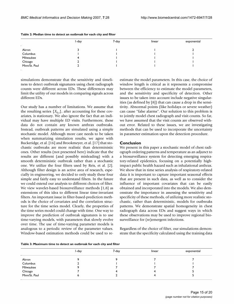
Tables 2 and 3 display, respectively, the median and max-imum detection times for each filter and city for ourmodel. The 1-day filter performed poorly. The other filtersare more comparable. We observed (results not shown)that the time to detection increases if the attack rate isreduced and also if the probabilities of entering the ED isdelayed.

We now compare the performance of our model, asdefined by equation (1), with three other models, in orderto investigate the effect of different covariates and timeseries components upon outbreak signature detection.Remember {Rk,t} are the number of chest radiographs forthe ED in city k on day t, {Vk,t} are the ED visit counts, and{Tk,t} are the thirty day smoothed time series of tempera-ture. For each day, t, and day of the week, d = 1, ..., 7, letDd,t be an indicator function that is one if that day is thedth day of the week, and zero otherwise. The four modelswe compare are:

1. Our covariates plus SARIMA errors model: Rk,t = β0,k +βV,kVk,t + βT,kTk,t + Xk,t, where {Xk,t} is the SARIMA modelused in the Results section.

2. Covariates (with seasonality) with autoregressive mov-ing average (ARMA) errors model:

,

where {Xk,t} is an ARMA model (equation (4), without

the Φk and Θk terms) with orders pk = 1 and qk = 1. Instead

of modeling the weekly effect using a random seasonalcomponent we use day-of-the week as a fixed effect (cov-ariate).

3. Covariates and no time series errors:

,

R V T D Xk t k V t k t T k k t D d k d td k t, , , , , , , , , ,= + + + +=∑β β β β0 16

R V T D Xk t k V t k t T k k t D d k d td k t, , , , , , , , , ,= + + + +=∑β β β β0 16

Quantiles of the chest radiograph distribution attributable to an anthrax outbreakFigure 4Quantiles of the chest radiograph distribution attrib-utable to an anthrax outbreak. Plots of the day-by-day quantiles of the radiograph counts attributable to an anthrax attack, based on 500 simulated anthrax outbreaks.

05

1015

20

weeks since outbreak

attr

ibut

able

che

st r

adio

grap

hs

0 1 2 3 4 5 6 7 8 9 10

0.975 quantilemedian0.025 quantile



where {Xk,t} is a mean zero white noise process with inno-

vation variance .

4. No covariates and ARMA errors: Rk,t = β0,k + Xk,t, where{Xk,t} is the same ARMA model as in Model 2.

Figure 8 displays the difference of actual specificity (calcu-lated using the training data) and the nominal specificity(the predetermined 1 - α) for different values of α forthese four models. For illustration we use the linear filter,which represents a compromise between the actual specif-icity and sensitivity (Across all four models, the 1-day fil-ter always had specificities closest to nominal and the 7-

σk2

Quantiles of the filtered chest radiograph distribution attributable to an anthrax outbreakFigure 5Quantiles of the filtered chest radiograph distribution attributable to an anthrax outbreak. Plots of the day-by-day quantiles of the filtered radiograph counts attributable to an anthrax attack, based on 500 simulated anthrax outbreaks. The filtering operation, as defined by (3), is based on the first ten months of training data from Akron, in combination with one of four filters (1-day, 7-day, linear and exponential). Each filtered signal is scaled by τk, 0.03, calculated using a normal approxima-tion, for comparisons to be made across filters.

−2

02

46

810

1−day filter


extr

a fil

tere

d ra

diog

raph

cou

nts

0 1 2 3 4 5 6 7 8 9 10

0.975 quantilemedian0.025 quantile

−2

02

46

810

7−day filter

weeks since outbreakex

tra

filte

red

radi

ogra

ph c

ount

s

0 1 2 3 4 5 6 7 8 9 10

−2

02

46

810

linear filter


extr

a fil

tere

d ra

diog

raph

cou

nts

0 1 2 3 4 5 6 7 8 9 10

−2

02

46

810

exponential filter


extr

a fil

tere

d ra

diog

raph

cou

nts

0 1 2 3 4 5 6 7 8 9 10




The biases in the specificityFigure 6The biases in the specificity. A plot of the actual specificity (the specificity calculated using the training data) minus the nominal specificity (1 - α) for different values of α. The value of the detection threshold τk,α, was calculated using a normal approximation.

0.02 0.04 0.06 0.08 0.10

−0.

050.

000.

05

One minus the nominal specificity, α

Act

ual m

inus

nom

inal

Akron

7−daylinearexponential1−day

0.02 0.04 0.06 0.08 0.10

−0.

050.

000.

05


Act

ual m

inus

nom

inal

Columbus

0.02 0.04 0.06 0.08 0.10

−0.

050.

000.

05


Act

ual m

inus

nom

inal

Milwaukee

0.02 0.04 0.06 0.08 0.10

−0.

050.

000.

05


Act

ual m

inus

nom

inal

Chicago

0.02 0.04 0.06 0.08 0.10

−0.

050.

000.

05


Act

ual m

inus

nom

inal

MinnStPaul



Receiver operating characteristic curvesFigure 7Receiver operating characteristic curves. Receiver operating characteristic curves (averaged over 500 simulations of an anthrax outbreak) for the detection of the anthrax outbreak signature in the chest radiographs at each of the five metropolitan children's hospitals.

0.04 0.06 0.08 0.10 0.12

0.2

0.4

0.6

0.8

1.0

One minus the actual specificity

Mea

n se

nsiti

vity

Akron

7−daylinearexponential1−day

0.04 0.06 0.08 0.10 0.12 0.14

0.98

00.

990

1.00

0


Mea

n se

nsiti

vity

Columbus

0.03 0.05 0.07 0.09

0.4

0.6

0.8

1.0


Mea

n se

nsiti

vity

Milwaukee

0.02 0.04 0.06 0.08 0.10 0.12

0.4

0.6

0.8

1.0


Mea

n se

nsiti

vity

Chicago

0.02 0.04 0.06 0.08 0.10 0.12 0.14

0.5

0.7

0.9


Mea

n se

nsiti

vity

MinnStPaul


day filter had specificities furthest away). Except forColumbus, Model 1 achieved a specificity closer to thenominal value across all EDs (Model 3 outperformsModel 1 in Columbus). Except in Chicago, Model 4 hadthe largest magnitude of bias.

Figure 9 compares the receiver operator characteristic(ROC) curves for the four models across the five EDsusing the linear filter (Across all models, the sensitivity forthe 1-day filter was the lowest while the 7-day and linearfilters tended to have the highest sensitivity). To readilycompare the models, we use one minus the nominal spe-cificity on the x-axis. Except for Akron and Minneapolis/St. Paul, the random weekly and daily time series compo-nents in Model 1 yield higher sensitivities, compared toincluding a day-of-week covariate plus ARMA errors inModel 2, and day-of-week covariate plus no ARMA errorsin Model 3. This is due to the insignificance of the day-of-week fixed effect in Models 2 and 3. In Akron, Model 3 hashigher sensitivities than Model 1, suggesting that the timeseries errors are less relevant in outbreak signature detec-tion for the test data. In Minneapolis/St. Paul Models 1, 2,and 3 have equivalent sensitivities. Across all cities eitherModel 2 or Model 4 had the lowest sensivities, indicatingthat these models are less reliable for outbreak signaturedetection.

In terms of sensitivity, except for Chicago, Model 3 tendedto outperform Model 2 for all filters in the cities we stud-ied. This is counter-intuitive, as we would expect that amodel that includes the significant ARMA time seriescomponent (Model 2) should outperform one that didnot contain any time series components (Model 3). Inpractice there is a tradeoff between estimation and predic-tion. Table 4 displays the Akaike information criterions(AICs) for the four models, fit to the training data of thefive EDs. For each ED, a smaller AIC denotes a model thatbetter fits the data. Model 3 performed better than Model2 in one-step-ahead predictions (Figure 9), but Model 2better explains the training data than Model 3 (Table 4).Using the AIC we find Model 1 fits best to the trainingdata, even though it does not always yield the highest sen-sitivity.

DiscussionOur intention in this study was to find a flexible set of sta-tistical models that could be applied across a number ofemergency departments. We employ time series modelsthat include covariates, such as patient visit counts andambient temperature, as well as random seasonal terms.We use chest-radiograph ordering data from emergencydepartments of five regional Midwest children's hospitalsto detect signatures of respiratory outbreaks. We includevisit counts series as a covariate in the chest radiographmodel to account for variations due to, for example, ED

sizes, changes of staff within the ED, and even some sea-sonalities across the time period of interest. We use thetemperature series as a surrogate measure of the influenzaseason – the colder months in the western hemisphere.This is a more accurate measure of the influenza seasonthan using a fixed covariate such as a sinusoid. To reflectuncertainty in the variation of the influenza backgroundover seasons, these models allow for randomness in theseasonal components. The use of random seasonal com-ponents is an advantage over traditional fixed effect mod-els, since temporal patterns are not assumed to repeatprecisely the same way. Thus, signature detection capabil-ities are improved for the majority of EDs – sensitivity ishigher. For increased accuracy and timeliness, the use ofour model for the data analysis should represent one com-ponent of an integrated detection system. Once a signal istriggered by any of our models, we recommend the use ofclinical follow-up to corroborate or refute the emergenceof a bona fide epidemic. For example, radiographs andmedical charts will need to be reviewed to identify highlyanomalous findings or groupings of aberrant findings thatwould be expected to be present at early stages of out-breaks. We believe that the approach utilized in this workwill aid in this process and is more appropriate than mod-els using fixed periodicities that do not have the ability tocapture the underlying variabilities across seasons.

Of note, our study shows that there are similarities in thechest radiographs series from different EDs that can, forthe most part, be modeled by similar time series models.Similarities of the time series model across EDs have anumber of ramifications for detection of outbreak signa-tures. First, by borrowing information across the differentEDs we can build more complicated multivariate timeseries models, possibly involving the joint modeling ofchest radiograph and visit counts across locations. Sec-ond, we could use these models to jointly detect outbreaksignatures across large spatial regions. In this context, Dig-gle et al. [20] use spatio-temporal Cox models to identifyanomalies (real and artificial outbreaks) in the space-timedistribution of gastrointestinal infections. But, some cau-tion is needed because one potential drawback of aggre-gating data spatially is that the chance of detection can bereduced (data from unaffected areas will mask the out-break signature, and increase the detection time) [21]. Forlocalized outbreaks, there is still some utility in buildingmodels that borrow strength across EDs, even if the jointdetection of outbreak signatures is not meaningful. Interms of these localized outbreaks, a geographically closesite could act as a benchmark to judge detections at othersites. For example, under certain circumstances an epi-demic detection signal triggered in Columbus, but not inAkron, could imply that some unusual event had occurredin Columbus. It should be noted, however, that eventhough there are similarities in the time series models, our



simulations demonstrate that the sensitivity and timeli-ness to detect outbreak signatures using chest radiographcounts were different across EDs. These differences maylimit the utility of our models in comparing signals acrossdifferent EDs.

Our study has a number of limitations. We assume thatthe resulting series {Xk,t}, after accounting for these cov-ariates, is stationary. We also ignore the fact that an indi-vidual may have multiple ED visits. Furthermore, thesedata do not contain any known anthrax outbreaks.Instead, outbreak patterns are simulated using a simplestochastic model. Although more care needs to be takenwhen summarizing simulation results, we agree withBuckeridge, et al. [16] and Brookmeyer, et al. [17] that sto-chastic outbreaks are more realistic than deterministicones. Other results (not presented here) indicate that theresults are different (and possibly misleading) with asmooth deterministic outbreak rather than a stochasticone. We utilize the four filters used by Reis, et al. [2].Although filter design is an active area of research, espe-cially in engineering, we decided to only study these foursimple and fairly easy to understand filters. In the futurewe could extend our analysis to different choices of filter.We view wavelet-based biosurveillance methods [1,8] asextensions of this idea to different linear time-invariantfilters. An important issue in filter-based-prediction meth-ods is the choice of covariates and the correlation struc-ture for the time series model. Clearly, the properties ofthe time series model could change with time. One way toimprove the prediction of outbreak signatures is to usetime-varying models, with parameters that slowly evolveover time. The use of time-varying parameter models isanalogous to a periodic review of the parameter values.Window-based estimation methods could be used to re-

estimate the model parameters. In this case, the choice ofwindow length is critical as it represents a compromisebetween the efficiency to estimate the model parameters,and the sensitivity and specificity of detection. Otherissues to be taken into account include negative singular-ities (as defined by [8]) that can cause a drop in the sensi-tivity. Abnormal points (like holidays or severe weather)can cause "false alarms". Our solution to this problem isto jointly model chest radiograph and visit counts. So far,we have assumed that the visit counts are observed with-out error. Related to these issues, we are investigatingmethods that can be used to incorporate the uncertaintyin parameter estimation upon the detection procedure.

ConclusionWe present in this paper a stochastic model of chest radi-ograph ordering patterns and temperature as an adjunct toa biosurveillance system for detecting emerging respira-tory-related epidemics, focusing on a potentially high-impact public health hazard such as inhalational anthrax.We show that in time series analysis of respiratory-relateddata it is important to capture important seasonal effectsthat are present in such data, as well as to consider theinfluence of important covariates that can be easilyobtained and incorporated into the models. We also dem-onstrate the importance in assessing the sensitivity andspecificity of these methods, of utilizing more realistic sto-chastic, rather than deterministic, models for outbreakspatterns. We demonstrate spatial homogeneity in chestradiograph data across EDs and suggest ways in whichthese observations may be used to improve regional bio-surveillance for (re)emergent infections.

Regardless of the choice of filter, our simulations demon-strate that the specificity calculated using the training data

Table 2: Median time to detect an outbreak for each city and filter

1-day 7-day linear exponential

Akron 3 1 1 2Columbus 1 1 1 1Milwaukee 4 1 1 1Chicago 2 1 1 1Minn/St. Paul 2 1 1 1

Table 3: Maximum time to detect an outbreak for each city and filter

1-day 7-day linear exponential





The biases in the specificity for the four modelsFigure 8The biases in the specificity for the four models. A plot of the actual specificity (the specificity calculated using the train-ing data) minus the nominal specificity (1 - α) for different values of α using a linear filter, for four different models. The value of the detection threshold τk,α, was calculated using a normal approximation.

0.02 0.04 0.06 0.08 0.10

−0.

5−

0.3

−0.

1


Act

ual m

inus

nom

inal

Akron

0.02 0.04 0.06 0.08 0.10

−0.

5−

0.3

−0.

1


Act

ual m

inus

nom

inal

Columbus

0.02 0.04 0.06 0.08 0.10

−0.

5−

0.3

−0.

1


Act

ual m

inus

nom

inal

Milwaukee

0.02 0.04 0.06 0.08 0.10

−0.

5−

0.3

−0.

1


Act

ual m

inus

nom

inal

Chicago

Model 1Model 2Model 3Model 4

0.02 0.04 0.06 0.08 0.10

−0.

5−

0.3

−0.

1


Act

ual m

inus

nom

inal

MinnStPaul



Receiver operating characteristic curves for the four modelsFigure 9Receiver operating characteristic curves for the four models. Receiver operating characteristic curves (averaged over 500 simulations of an anthrax outbreak) for the detection of the anthrax outbreak signature in the chest radiographs at each of the five metropolitan children's hospitals using the four different models. The linear filter is used in each case.

0.02 0.04 0.06 0.08 0.10

0.2

0.4

0.6

0.8

1.0

One minus the nominal specificity

Mea

n se

nsiti

vity

Akron

0.02 0.04 0.06 0.08 0.10

0.2

0.4

0.6

0.8

1.0


Mea

n se

nsiti

vity

Columbus

0.02 0.04 0.06 0.08 0.10

0.2

0.4

0.6

0.8

1.0


Mea

n se

nsiti

vity

Milwaukee

0.02 0.04 0.06 0.08 0.10

0.2

0.4

0.6

0.8

1.0


Mea

n se

nsiti

vity

Chicago

Model 1Model 2Model 3Model 4

0.02 0.04 0.06 0.08 0.10

0.2

0.4

0.6

0.8

1.0


Mea

n se

nsiti

vity

MinnStPaul


varied across the five EDs studied (Figure 6). The tradeoffbetween specificity and sensitivity also varied by the ED(Figures 6 and 7). The 1-day filter, while closely matchingthe nominal specificity, performed poorly in terms ofmaximizing the sensitivity to detect an outbreak signa-ture. The 7-day filter, by smoothing over the outbreak sig-nature (Figure 5), maximized the sensitivity, but at acompromise to the actual specificity obtained (Figures 6and 7). The linear and exponential filters provided a bal-ance between the specificity and sensitivity. Detectionusing our covariate-based seasonal time series model per-formed well across all EDs compared with fixed-effectsregression models or time series models that omitted sea-sonal terms and/or covariates (Figures 8 and 9).

Competing interestsThe author(s) declare that they have no competing inter-ests.

Authors' contributionsDr. Bonsu provided the motivation, scientific back-ground, and data for this work. Under supervision, N.Kim developed the preliminary simulation model for ananthrax attack. Dr. Craigmile worked on the filtering the-ory used in the paper, and together with N. Kim and Dr.Fernandez analyzed the data, planned and carried out thesimulations, and wrote the paper. Dr. Craigmile took thelead with writing. All authors jointly edited this work.

AppendixThe SARIMA modelIn city k, we define a SARIMA (pk, 0, qk) × (Pk, 0, Qk) withperiod of seasonality s for the time series {Xk,t} using thenotation of Section 6.5 of Brockwell and Davis [19]. Let-ting B denote the backshift operator defined by BrZk,t = Br-

1 Zk,t-1 for r > 0, with B0 Zk,t = Zk,t, we define Xk,t by

φk(B)Φk(Bs)Xk,t = θk(B)Θk(Bs)Zk,t.

In this model the parameter s denotes the period of theseasonality. The characteristic polynomials for theSARIMA model are

The terms φk(z) and θk(z) define an autoregressive movingaverage process on the unit time scale, whereas the termsΦk(z) and Θk(z) define an autoregressive moving averageprocess on a time scale of s units. Thus we can modeldependencies simultaneously on two different time

scales. It is customary to restrict to the class of causal timeseries models (e.g., [[19], Chapter 2]). The SARIMA modelis causal (i.e., can be represented in terms of a movingaverage (MA) process of only past events) if φk(z) ≠ 0 andΦk(z) ≠ 0, for complex valued z such that |z| ≤ 1.

To complete the model we assume that {Zk,t} is a mean

zero white noise process with innovation variance .

FilteringA discrete-time filter is a set of coefficients, {fl : l = ..., -2, -1, 0, 1, 2, ...}, where ∑l|fl| < ∞. The new time series {Yt}obtained by filtering the time series {Xt} using {fl} isdefined by the convolution

for each t. The actual operation that a filter carries outupon a time series depends on the values of the filter coef-ficients. Simple examples of a filter include the differenc-ing filter defined by

which corresponds to Yt = Xt - Xt-1 for each t, and the sim-ple moving average filter of length 2M + 1 whose filter isdefined by

Thus, , for each t.

Suppose that the radiograph series {Rk,t} follows a timeseries model given by (1). Let γX,k(·) denote the autocov-ariance function of the stationary error component {Xk,t}.Consider only the last m values of the process Rk,t, {Rk,t-1,..., Rk,t-m}. Given the model parameters, by linearity of theprediction operator, the best linear one-step predictor ofRk,t is given by

where

φ φ φ

θ

k k k pp

k k k PP

k

z z z

z z z

z

kk

KK

( ) ;

( ) ;

( )

, ,

, ,

= − − −

= − − −

= +

1

1

1

1

1

…

…Φ Φ Φ

θθ θk k qq

k k k QQ

z z

z z z

KK

KK

, ,

, ,

;

( ) .

1

11

+ +

= + + +

…

…Θ Θ Θ

σk2

Y f Xt l t ll

= −=−∞

∞∑ ,

f

l

ll ==

− =⎧⎨⎪

⎩⎪

1 0

1 1

0

;

;

,otherwise

fM l M M

l =+ = −⎧

⎨⎩

1 2 1

0

/( ) ,..., ;

.otherwise

Y M Xt t ll MM= + −

+=−∑( )2 1 1

ˆ ˆ, , , , , , ,R V T Xk t t V k k t T k k t k t= + + +β β β0 (5)

ˆ ,, , ,X b Xk t k j k t jj

m= −

=∑

1

(6)



denotes the one-step ahead prediction for the SARIMAprocess and {bk,1, ..., bk,m} are obtained from the solutionof the set of m linear equations:

The one-step prediction error process, {Ek,t} is

where we define ck,0 = 1 and ck,j = -bk,j for j = 1, ..., m. Theprocess {Ek,t} is a filtering of {Xk,t} and so if {Xk,t} is sta-tionary, by the linear time invariant filtering result for sta-tionary processes, {Ek,t} is also stationary ([18], Theorem4.10.1). Moreover for large enough m, if {Xk,t} is an invert-ible time series process then we can approximate {Xk,t} byan autoregressive, AR(m) process ([18], Theorem 4.4.3).Using this approximation we can argue that {Ek,t} isapproximately a mean zero Gaussian independent andidentically distributed process with variance gammaγX,k(0).

Let {a0, ..., aL-1} denote a pre-specified filter of width L. Wedefine the detection process {Dk,t} by filtering the errorprocess {Ek,t} using this filter. Thus,

By the filtering result for stationary processes, stationarityof {Xk,t} implies that {Dk,t} is also a stationary process.

For large enough m, since {Ek,t} is approximately a white

noise process,{Dk,t} is approximately a moving average

process of order L - 1 with coefficients θ0 = 1, θj = aj-1/a0 for

j = 1, ..., L - 1, and innovation variance .

We declare evidence of an outbreak signature (test posi-tive), at time t if the observed detection value Dk,t is largerthan a given threshold. For a fixed value of α, let 1 - αdenote the specificity (the probability of a true-negative).Similarly, the sensitivity is defined to be the probability of

true positive. The threshold, τk,α, is chosen by solving P(Dk,t > τk,α) = α for τk,α. Either we can estimate this valuefrom the data using the 1 - α quantile of the {Dk,t} processof non-outbreak-based training data, or if {Xk,t} is Gaus-sian then for large m,

where Z is a standard normal random variable. The solu-tion for the threshold under this approximation is

where Φ-1(·) denotes the inverse cumulative distributionfunction for a standard normal random variable.

The filter-based detection method requires knowledge ofthe "true" values of the model parameters. In our work, wereplace the parameters with their maximum likelihoodestimates.

AcknowledgementsWe would like to thank Elaine Damo at Columbus Children's Hospital for collecting the data, and Dr. Steven MacEachern for helpful discussions about our work. We also thank the two referees for their extensive com-ments that improved this article.

References1. Shmueli G: Wavelet-Based Monitoring in Modern Biosurveil-

lance. Tech rep 2005 [http://www.rhsmith.umd.edu/faculty/gshmueli/biosurveillance2005.pdf]. Smith School of Business, University of Mar-yland

2. Reis B, Pagano M, Mandl K: Using temporal context to improvebiosurveillance. Proceedings of the National Academy of Sciences2003, 100(4):1961-1965.

3. Reis B, Mandl K: Time series modeling for syndromic surveil-lance. BMC Medical Informatics and Decision Making 2003, 3(2):[http://www.biomedcentral.com/1472-6947/3/2].

4. Mandl K, Overhage J, Wagner M, Lober W, Sebastiani P, MostashariF, Pavlin J, Gesteland P, Treadwell T, Koski E, Hutwagner L, Buck-eridge D, Aller R, Grannis S: Syndromic surveillance: a guideinformed by the early experience. Journal of the American MedicalInformatics Association 2004, 11(2):141-150.

γ γX k k j X kj

mh b h j h m, , ,( ) ( ), ,..., .= − =

=∑

1

1 (7)

E R R X X X b X c Xk t k t k t k t k t k t k j k t j k j k t jj

m

, , , , , , , , , ,= − = − = − =− −=∑

0jj

m

=∑

1

,

D a Ek t h k t hh

L

, , .= −=

−∑

0

1(8)

a X k02 0γ , ( )

P D P Za

k t kk

X k hhL

( )( )

,, ,,

,

> ≈ >⎛

⎝

⎜⎜⎜

⎞

⎠

⎟⎟⎟

=

=−∑

ττ

γαα

α

0 201

(9)

τ γ ααk X k hh

La, ,

/

( ) ( ),=⎛

⎝⎜⎜

⎞

⎠⎟⎟ −

=

−−∑0 12

0

1 1 21Φ (10)

Table 4: Akaike information criterions (AICs) for Models 1–4 fit to the training data for each ED

City Model 1 Model 2 Model 3 Model 4



http://www.rhsmith.umd.edu/faculty/gshmueli/biosurveillance2005.pdf

http://www.rhsmith.umd.edu/faculty/gshmueli/biosurveillance2005.pdf

http://www.biomedcentral.com/1472-6947/3/2




Publish with BioMed Central and every scientist can read your work free of charge

"BioMed Central will be the most significant development for disseminating the results of biomedical research in our lifetime."

Sir Paul Nurse, Cancer Research UK

Your research papers will be:

available free of charge to the entire biomedical community

peer reviewed and published immediately upon acceptance

cited in PubMed and archived on PubMed Central

yours — you keep the copyright

Submit your manuscript here:http://www.biomedcentral.com/info/publishing_adv.asp

BioMedcentral

5. Box GEP, Luceno A: Statistical control by monitoring and feedback adjust-ment New Jersey: John Wiley and Sons; 1997.

6. Ivanov O, Gesteland P, Hogan W, Mundorff M, Wagner M: Detec-tion of Pediatric Respiratory and Gastrointestinal Outbreaksfrom Free-Text Chief Complaints. In Proceedings of the AnnualFall Symposium of the American Medical Informatics Association Madison:Omni Press; 2003:318-322.

7. Burkom HS, Elbert Y, Feldman A, Lin J: Role of data aggregationin biosurveillance detection strategies with applicationsfrom essence. Morbidity and Mortality Weekly Report (MMWR) 2004,53:67-73.

8. Zhang J, Tsui FC, Wagner M, Hogan W: Detection of PediatricRespiratory and Gastrointestinal Outbreaks from Free-TextChief Complaints. In Proceedings of the Annual Fall Symposium of theAmerican Medical Informatics Association Madison: Omni Press;2003:748-752.

9. Naumova EN, O'Neil E, MacNeill I: A System for Early OutbreakDetection and Signature Forecasting. Morbidity and MortalityWeekly Report 2005, 54:77-83.

10. Ismail N, Pettitt A, Webster R: 'Online' monitoring and retro-spective analysis of hospital outcomes based on a scan statis-tic. Statistics in Medicine 2003, 22:2861-2876.

11. Wallenstein S, Naus J: Scan Statistics for Temporal Surveillancefor Biologic Terrorism. Morbidity and Mortality Weekly Report2004, 53:74-78.

12. Naus J, Wallenstein S: Temporal Surveillance Using Scan Sta-tistics. Statistics in Medicine 2006, 25:311-324.

13. Jackson ML, Baer A, Painter I, Duchin J: A simulation study com-paring aberration detection algorithms for syndromic sur-veillance. BMC Medical Informatics and Decision Making 2007, 7(6):[http://www.pubmedcentral.nih.gov/articlerender.fcgi?tool=pubmed&pubmedid=17331250].

14. Brillman JC, Burr T, Forslund D, Joyce E, Picard R, Umland E: Mode-ling emergency department visit patterns for infectious dis-ease complaints: results and application to diseasesurveillance. BMC Medical Informatics and Decision Making 2005,5(4): [http://www.biomedcentral.com/1472-6947/5/4/].

15. Average Daily Temperature Archive at The University ofDayton [http://www.engr.udayton.edu/weather/citylistUS.htm]

16. Buckeridge D, Burkom H, Moore A, Pavlin J, Cutchis P, Hogan W:Evaluation of syndromic surveillance systems – design of anepidemic simulation model. Morbidity and Mortality Weekly Report2004, 53:137-143 [http://www.cdc.gov/mmwr/pdf/wk/mm53su01.pdf].

17. Brookmeyer R, Johnson E, Barry S: Modelling the incubationperiod of anthrax. Statistics in Medicine 2005, 24:531-542.

18. Brockwell PJ, Davis RA: Time Series. Theory and Methods. Sec-ond edition. New York: Springer-Verlag; 1991.

19. Brockwell PJ, Davis RA: Introduction to time series and fore-casting. Second edition. New York: Springer-Verlag; 2002.

20. Diggle P, Rowlingson B, Su T: Point process methodology for on-line spatio-temporal disease surveillance. Environmetrics 2005,16(5):423-434.

21. Fienberg S, Shmueli G: Statistical Issues and Challenges Associ-ated with Rapid Detection of Bio-terrorist Attacks. Statisticsin Medicine 2005, 24(4):513-529.

Pre-publication historyThe pre-publication history for this paper can be accessedhere:

http://www.biomedcentral.com/1472-6947/7/28/prepub







http://www.pubmedcentral.nih.gov/articlerender.fcgi?tool=pubmed&pubmedid=17331250

http://www.pubmedcentral.nih.gov/articlerender.fcgi?tool=pubmed&pubmedid=17331250

http://www.biomedcentral.com/1472-6947/5/4/

http://www.engr.udayton.edu/weather/citylistUS.htm

http://www.cdc.gov/mmwr/pdf/wk/mm53su01.pdf

http://www.cdc.gov/mmwr/pdf/wk/mm53su01.pdf





http://www.biomedcentral.com/1472-6947/7/28/prepub


http://www.biomedcentral.com/info/publishing_adv.asp


Modeling and detection of respiratory-related outbreak signatures

Documents

Transcript of Modeling and detection of respiratory-related outbreak signatures