Modeling and Description of Embedded Processors for the ...
206
Modeling and Description of Embedded Processors for the Development of Software Tools Wei Qin A DISSERTATION PRESENTED TO THE FACULTY OF PRINCETON UNIVERSITY IN CANDIDACY FOR THE DEGREE OF DOCTOR OF PHILOSOPHY RECOMMENDED FOR ACCEPTANCE BY THE DEPARTMENT OF ELECTRICAL ENGINEERING November 2004
-
Upload
khangminh22 -
Category
Documents
-
view
1 -
download
0
Transcript of Modeling and Description of Embedded Processors for the ...
Modeling and Description of Embedded Processors
for the Development of Software Tools
Wei Qin
A DISSERTATION
PRESENTED TO THE FACULTY
OF PRINCETON UNIVERSITY
IN CANDIDACY FOR THE DEGREE
OF DOCTOR OF PHILOSOPHY
RECOMMENDED FOR ACCEPTANCE
BY THE DEPARTMENT OF
ELECTRICAL ENGINEERING
November 2004

c© Copyright by Wei Qin, 2004.
All rights reserved.
Abstract
Increasing design and manufacturing costs are prompting a shift in electronic design
from hardwired application-specific integrated circuits (ASICs) to the use of software
on programmable platforms. In order to minimize the power and performance over-
head of such platforms, domain or application-specific processors have been used.
The development of such processors requires not only traditional electronic design
automation tools but also processor-specific software tools such as compilers and in-
struction set simulators. In early development stages when multiple processor design
points are explored, it is necessary to have the software tools synthesized from high
level processor descriptions. This dissertation presents an approach that aims to
automate the synthesis of these software tools. The foundation of the approach is
a novel concurrency model, the operation state machine (OSM). The OSM model
views a processor in two interacting levels: the operation level where instruction be-
havior is represented and the hardware level where resources required for instruction
execution are managed. Through proper abstraction, the model significantly sim-
plifies the specification of concurrency and control semantics without compromising
flexibility. This dissertation then presents the MESCAL Architecture Description
Language (MADL) which is designed using the OSM model. It describes the major
design considerations of MADL and the synthesis of software tools including cycle-
iii
accurate simulators, instruction set simulators, disassemblers, and binary decoders
from MADL-based processor models. It further goes on to show how this description
can be used to extract reservation tables for use in instruction schedulers in compil-
ers. Experimental results show that the MADL-based approach is very effective in
supporting these software tools and the synthesized cycle-accurate simulators have
competitive simulation speeds compared to their hand-coded counterparts.
iv
Acknowledgements
First of all, I would like to thank my thesis adviser, Professor Sharad Malik, for the
guidance that he has given me during the past five years. Without Professor Malik’s
extraordinary vision, enthusiasm, and patience, this thesis work would not have been
possible. I truly enjoyed my experience working with him.
I am grateful to Professor Malik, Professor Wayne Wolf and Professor David
August for taking their time to read the thesis and providing invaluable improvement
suggestions. I am also obliged to Professor Ruby Lee, Professor Margaret Martonosi,
and Professor Stephen Edwards for their generous help in my research and career
pursuit. I thank the faculty and staff of the Princeton University Department of
Electrical Engineering for all the help and advice that they gave me in the past five
years.
I thank all members of the MESCAL project for the help and discussions that
improved the quality of the thesis work. I also thank members of the Liberty group
whose insightful opinions greatly helped me to refine the main idea of the thesis.
I thank all my friends for all their help and for their making my life enjoyable in
Princeton.
Finally, I would like to thank my family. My parents and my brother have been
a continuous source of support throughout my life, even when they are thousands of
v
miles away. My wife Mujun accompanied me throughout the course of my graduate
study and kept my life organized. She also helped to improve my writing skills and
proof-read the draft of the thesis. My lovely daughter Lillian came to this world just
in time to make my thesis writing a more challenging task, but also more meaningful.
I dedicate this thesis to all of them.
This research was supported by the MESCAL project of the Gigascale Silicon
Research Center (GSRC).
vi
Contents
Abstract iii
Acknowledgements v
Contents vii
List of Figures xii
List of Tables xiv
1 Introduction 1
1.1 Overview of Modern Electronic System Design . . . . . . . . . . . . . 1
1.2 Platform-Based Design . . . . . . . . . . . . . . . . . . . . . . . . . . 7
1.3 Software Programmable Platforms . . . . . . . . . . . . . . . . . . . . 8
1.4 Terminology . . . . . . . . . . . . . . . . . . . . . . . . . . . . . . . . 12
1.5 Dissertation Overview . . . . . . . . . . . . . . . . . . . . . . . . . . 12
2 Related Work 16
2.1 Introduction . . . . . . . . . . . . . . . . . . . . . . . . . . . . . . . . 16
2.2 Survey of Architecture Modeling Approaches . . . . . . . . . . . . . . 18
2.2.1 Discrete Event Model . . . . . . . . . . . . . . . . . . . . . . . 18
vii
2.2.2 Synchronous Structural Models . . . . . . . . . . . . . . . . . 21
2.2.3 Synchronous Behavioral Model . . . . . . . . . . . . . . . . . 23
2.2.4 Abstract State Machine Model . . . . . . . . . . . . . . . . . . 24
2.2.5 Domain-specific Model . . . . . . . . . . . . . . . . . . . . . . 25
2.2.6 Architecture Templates . . . . . . . . . . . . . . . . . . . . . . 27
2.2.7 Formal Mathematical Models . . . . . . . . . . . . . . . . . . 30
2.2.8 Other Work . . . . . . . . . . . . . . . . . . . . . . . . . . . . 32
2.2.9 Summary of Architecture Models . . . . . . . . . . . . . . . . 32
2.3 Architecture Description Schemes . . . . . . . . . . . . . . . . . . . . 36
2.3.1 Structure Description Techniques . . . . . . . . . . . . . . . . 36
2.3.2 Instruction Description Techniques . . . . . . . . . . . . . . . 37
2.4 Summary . . . . . . . . . . . . . . . . . . . . . . . . . . . . . . . . . 39
3 Architecture Model 41
3.1 Introduction . . . . . . . . . . . . . . . . . . . . . . . . . . . . . . . . 41
3.2 Problem Definition: Modeling Concurrency . . . . . . . . . . . . . . . 44
3.3 Operation State Machine Model . . . . . . . . . . . . . . . . . . . . . 47
3.3.1 Abstractions . . . . . . . . . . . . . . . . . . . . . . . . . . . . 48
3.3.2 OSM Model . . . . . . . . . . . . . . . . . . . . . . . . . . . . 50
3.3.3 Modeling Details . . . . . . . . . . . . . . . . . . . . . . . . . 57
3.3.4 Modeling of Common Processor Features . . . . . . . . . . . . 63
3.3.5 Scheduling . . . . . . . . . . . . . . . . . . . . . . . . . . . . . 69
3.4 Discussions on Scheduling . . . . . . . . . . . . . . . . . . . . . . . . 74
3.5 Discussions of the OSM Model . . . . . . . . . . . . . . . . . . . . . . 78
3.6 Comparison with Other Architecture Models . . . . . . . . . . . . . . 81
viii

3.7 Summary . . . . . . . . . . . . . . . . . . . . . . . . . . . . . . . . . 83
4 An Architecture Description Language for Generation of Software
Tools 85
4.1 Introduction . . . . . . . . . . . . . . . . . . . . . . . . . . . . . . . . 85
4.2 Core Language . . . . . . . . . . . . . . . . . . . . . . . . . . . . . . 89
4.2.1 Applying the AND-OR Graph Technique . . . . . . . . . . . . 90
4.2.2 Dynamic OSM Model . . . . . . . . . . . . . . . . . . . . . . . 92
4.2.3 Converting the Dynamic OSM model . . . . . . . . . . . . . . 97
4.2.4 Additional Actions . . . . . . . . . . . . . . . . . . . . . . . . 100
4.3 Annotations . . . . . . . . . . . . . . . . . . . . . . . . . . . . . . . . 100
4.4 Summary . . . . . . . . . . . . . . . . . . . . . . . . . . . . . . . . . 103
5 Synthesis of Software Development Tools 105
5.1 Introduction . . . . . . . . . . . . . . . . . . . . . . . . . . . . . . . . 105
5.2 Synthesis of the CAS . . . . . . . . . . . . . . . . . . . . . . . . . . . 107
5.2.1 Simplifications of the Simulation Kernel . . . . . . . . . . . . 109
5.2.2 Decoding Optimization . . . . . . . . . . . . . . . . . . . . . . 111
5.2.3 Experiments . . . . . . . . . . . . . . . . . . . . . . . . . . . . 112
5.3 Synthesis of the ISS . . . . . . . . . . . . . . . . . . . . . . . . . . . . 118
5.3.1 Procedure Generation . . . . . . . . . . . . . . . . . . . . . . 119
5.3.2 Experimental Results . . . . . . . . . . . . . . . . . . . . . . . 120
5.4 Synthesis of the Disassembler . . . . . . . . . . . . . . . . . . . . . . 123
5.5 Extraction of the Reservation Table . . . . . . . . . . . . . . . . . . . 124
5.6 Synthesis of the Binary Decoder . . . . . . . . . . . . . . . . . . . . . 128
5.6.1 Related Work . . . . . . . . . . . . . . . . . . . . . . . . . . . 129
ix
5.6.2 Problem Formulation . . . . . . . . . . . . . . . . . . . . . . . 131
5.6.3 Decision function . . . . . . . . . . . . . . . . . . . . . . . . . 134
5.6.4 Division of Decoding Entry Set . . . . . . . . . . . . . . . . . 135
5.6.5 Evaluation of Decision Function . . . . . . . . . . . . . . . . . 138
5.6.6 Further Pruning of Search Space . . . . . . . . . . . . . . . . 140
5.6.7 Experimental Results . . . . . . . . . . . . . . . . . . . . . . . 141
5.7 Summary . . . . . . . . . . . . . . . . . . . . . . . . . . . . . . . . . 147
6 Conclusions 149
6.1 Contributions . . . . . . . . . . . . . . . . . . . . . . . . . . . . . . . 150
6.2 Future Work . . . . . . . . . . . . . . . . . . . . . . . . . . . . . . . . 153
A The MESCAL Architecture Description Language V1.0 Reference
Manual 155
A.1 Introduction . . . . . . . . . . . . . . . . . . . . . . . . . . . . . . . . 155
A.2 Define Section . . . . . . . . . . . . . . . . . . . . . . . . . . . . . . . 158
A.3 Manager Section . . . . . . . . . . . . . . . . . . . . . . . . . . . . . 159
A.4 Machine Section . . . . . . . . . . . . . . . . . . . . . . . . . . . . . . 161
A.5 Function Section . . . . . . . . . . . . . . . . . . . . . . . . . . . . . 163
A.6 Operation Section . . . . . . . . . . . . . . . . . . . . . . . . . . . . . 165
A.7 Action Ordering . . . . . . . . . . . . . . . . . . . . . . . . . . . . . . 170
A.8 Data Types . . . . . . . . . . . . . . . . . . . . . . . . . . . . . . . . 173
A.9 Basic Operators . . . . . . . . . . . . . . . . . . . . . . . . . . . . . . 175
A.10 Modifiers . . . . . . . . . . . . . . . . . . . . . . . . . . . . . . . . . . 175
A.11 OSM Actions . . . . . . . . . . . . . . . . . . . . . . . . . . . . . . . 177
A.12 Annotation Syntax . . . . . . . . . . . . . . . . . . . . . . . . . . . . 178
x

References 181
xi
List of Figures
1.1 Rising mask set cost . . . . . . . . . . . . . . . . . . . . . . . . . . . 5
1.2 Spin count for ASICs . . . . . . . . . . . . . . . . . . . . . . . . . . . 6
1.3 Common architecture platforms . . . . . . . . . . . . . . . . . . . . . 8
2.1 Example AND-OR graph . . . . . . . . . . . . . . . . . . . . . . . . . 37
3.1 Standard design process of embedded processors . . . . . . . . . . . . 42
3.2 Example OSM for an out-of-order processor . . . . . . . . . . . . . . 49
3.3 An illegal OSM portion . . . . . . . . . . . . . . . . . . . . . . . . . . 54
3.4 Overall structure of the OSM model . . . . . . . . . . . . . . . . . . . 56
3.5 Example scalar processor . . . . . . . . . . . . . . . . . . . . . . . . . 57
3.6 Hardware level model for the example processor . . . . . . . . . . . . 58
3.7 OSM for the add operation . . . . . . . . . . . . . . . . . . . . . . . . 59
3.8 Comprehensive OSM for an instruction set . . . . . . . . . . . . . . . 64
3.9 Modeling general data forwarding . . . . . . . . . . . . . . . . . . . . 67
3.10 Augmented OSM with resetting capability . . . . . . . . . . . . . . . 68
3.11 Example model using arbiter . . . . . . . . . . . . . . . . . . . . . . . 70
3.12 OSM scheduling algorithm . . . . . . . . . . . . . . . . . . . . . . . . 73
3.13 Adapted DE scheduler for OSM . . . . . . . . . . . . . . . . . . . . . 74
xii
4.1 Token manager description in MADL . . . . . . . . . . . . . . . . . . 90
4.2 Static state diagram of the example instruction set . . . . . . . . . . 92
4.3 Example dynamic state diagram . . . . . . . . . . . . . . . . . . . . . 93
4.4 Example MADL description . . . . . . . . . . . . . . . . . . . . . . . 94
4.5 MADL description of the syntax operations . . . . . . . . . . . . . . 95
4.6 Merged static state diagram . . . . . . . . . . . . . . . . . . . . . . . 99
4.7 Annotation syntax in BNF . . . . . . . . . . . . . . . . . . . . . . . . 102
4.8 Annotation description example . . . . . . . . . . . . . . . . . . . . . 103
5.1 Cycle-accurate simulator synthesis framework . . . . . . . . . . . . . 108
5.2 StrongARM microarchitecture diagram . . . . . . . . . . . . . . . . . 113
5.3 OSM fragment modeling ldm . . . . . . . . . . . . . . . . . . . . . . . 114
5.4 Speed comparison of CASs . . . . . . . . . . . . . . . . . . . . . . . . 116
5.5 ISS procedure generation . . . . . . . . . . . . . . . . . . . . . . . . . 121
5.6 Overview of reservation table extraction from MADL . . . . . . . . . 126
5.7 Example pattern sets . . . . . . . . . . . . . . . . . . . . . . . . . . . 132
5.8 Example decoding tree . . . . . . . . . . . . . . . . . . . . . . . . . . 133
5.9 Example of division . . . . . . . . . . . . . . . . . . . . . . . . . . . . 137
5.10 Decoder statistics . . . . . . . . . . . . . . . . . . . . . . . . . . . . . 143
5.11 ISS Simulation speed using the synthesized decoders . . . . . . . . . . 144
xiii
List of Tables
2.1 Summary of the architecture models . . . . . . . . . . . . . . . . . . 34
2.2 Usage of the architecture models . . . . . . . . . . . . . . . . . . . . 35
3.1 Dependency between actions . . . . . . . . . . . . . . . . . . . . . . . 71
5.1 Model statistics . . . . . . . . . . . . . . . . . . . . . . . . . . . . . . 115
5.2 Execution time Comparison . . . . . . . . . . . . . . . . . . . . . . . 118
5.3 ISS Simulation speed . . . . . . . . . . . . . . . . . . . . . . . . . . . 120
5.4 Comparison of decoders . . . . . . . . . . . . . . . . . . . . . . . . . 145
A.1 Basic operators in MADL . . . . . . . . . . . . . . . . . . . . . . . . 176
A.2 Modifiers in MADL . . . . . . . . . . . . . . . . . . . . . . . . . . . . 177
A.3 Actions in MADL . . . . . . . . . . . . . . . . . . . . . . . . . . . . . 178
xiv
Chapter 1
Introduction
1.1 Overview of Modern Electronic System Design
Since the invention of the first transistor in 1947, modern electronic systems have been
steadily percolating into nearly every part of human life. Continuous innovation in
the electronic industry has created a push effect that fuels the growth of other sectors
such as medical instruments, mass media, military equipment, industrial automation,
etc. At the same time, the insatiable demand from these markets has created a
pull effect that helps the rapid advancement of the electronic industry. The pace
of electronic technology innovation over the past forty years is best characterized
by Moore’s Law – chip density doubles in every two years [37] – a result of the
persistent efforts of researchers and engineers. Such exponential growth rate of chip
density allows engineers to pack more complex functionality into a single chip with
improving efficiency in terms of area, power, and performance. Leading semiconductor
manufacturers are now capable of producing very sophisticated electronic system-on-
chips (SoCs). For example, NVIDIA recently shipped its high performance GeForce
1
2 CHAPTER 1. INTRODUCTION
6800 graphics processing unit which has more than 220 million transistors on a single
die [58]. The invention of such SoCs enables the creation of novel appliances that are
changing people’s everyday life around the globe.
Complementary metal-oxide semiconductor (CMOS) technology has been the pre-
dominant semiconductor technology since the mid-80s. Compared with its prede-
cessors, CMOS technology has the advantage of high density, low power, and low
manufacturing cost. In the CMOS age, lithography scaling is the major driving force
for technology improvement. As a result, technology generations are usually defined
according to the feature size of the lithography process. To stay along the density
curve projected by Moore’s Law, the feature size needs to be reduced at the rate
of 30% every couple of years. Currently, semiconductor manufacturers are gradually
transitioning from the 130nm to the 90nm technology, marking the advent of the
nanometer design era [41]. In this new era, designers and manufacturers are facing a
number of unprecedented system and silicon complexity challenges. A brief overview
of some toughest challenges is provided below.
• Power
Power consumption and the related thermal management issues of high-end
electronic systems have become an important concern for designers. For exam-
ple, the Itanium 2 processor (Madison) [54] consumes a maximum power of 130
watts. Such a high power budget creates stringent requirements for packaging
and cooling, which add substantial cost to the overall system.
Power consumption contains two components, dynamic power and static power.
Static power mainly contains leakage power for CMOS circuits. Although tech-
nology scaling reduces the dynamic power consumption per device, it increases

1.1. OVERVIEW OF MODERN ELECTRONIC SYSTEM DESIGN 3
the leakage power due to lower threshold voltages. For instance, the Madi-
son processor, which is fabricated using the 130nm process, dissipates 21% of
its power as leakage power. This reflects a 2.5 times increase from its sibling
McKinley fabricated using the 180nm process [54]. Leakage power will continue
to grow for nanometer-scale designs and may soon dominate dynamic power
according to some researchers [42]. Left unchecked, it may limit the overall
advantage of scaling.
• Variability
Variability has recently become an important concern to designers. Intel re-
cently revealed that the Pentium 4 Northwood processors fabricated using the
130nm process displayed a frequency variation of 30% and a leakage power vari-
ation of 5 to 10 times [23]. This created new problems for yield and quality
control.
The variability issue will get more serious in nanometer designs. At nanometer
scale, the effective length of the gate channel is only a few hundred times the
diameter of a silicon atom. And the gate-oxide is only several atoms thick. Con-
sequently, non-uniform distribution of the atoms or any random fluctuations in
the manufacturing process may significantly affect the electrical properties of
a device, posing a severe threat to the yield rate of nanometer scale circuits.
Furthermore, in operation, chips often have local hot spots with temperature
much higher than the ambient. Since the electrical properties of a device de-
pends on its operating temperature, such temperature fluctuation exacerbates
the problem.
4 CHAPTER 1. INTRODUCTION
• Reliability
The reliability issue involves both transient and permanent failures of the oper-
ation of a circuit. Although permanent failures may be controlled by adopting
more conservative design rules, in general, there is no good solution for transient
failures, or soft errors. In nanometer designs where the operating voltages are
low, the critical charge for a device to preserve its state has become so small
that radiation from impurities in the chip packaging may flip the state. Given
the large number of logic devices in a nanometer chip, the overall rate of such
transient errors can be significant, raising concerns for the design of mission-
critical electronic systems. Such a phenomenon is not news to memory designers
who have used error correction coding (ECC). However, logic designers are just
beginning to search for solutions to improve the robustness of circuits.
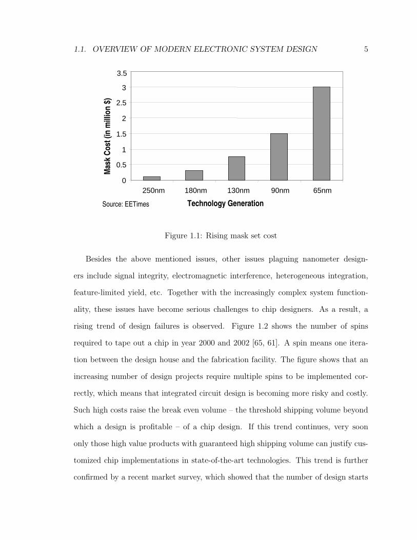
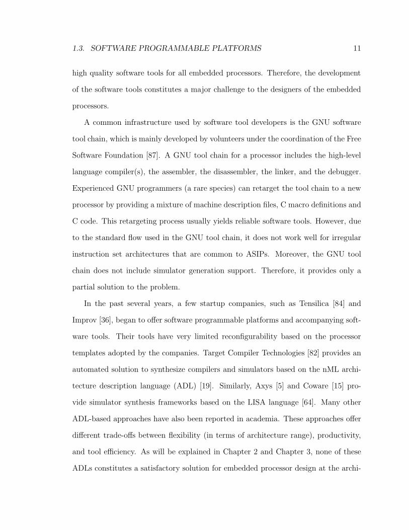
• Manufacturing Non-recurring Engineering (NRE) Cost.
Starting with the 180nm process, the process feature size becomes smaller
than the lithography wavelength. In such sub-wavelength lithography pro-
cesses, printed layout patterns are significantly affected by the local density
and neighborhood patterns. To pre-compensate for such distortion, resolution
enhancement techniques (RETs) were developed, including optical proximity
correction (OPC) and phase shift masking (PSM). These resolution enhance-
ment techniques make the traditional regular shapes on the masks drastically
more complex, therefore more expensive to produce. Figure 1.1 shows the typ-
ical mask set costs for high-end chips in different technologies [44]. The mask
set cost leaps from around $750,000 for 130nm technology to $1.5M for 90nm
technology. It is estimated that $3M is needed for a 65nm mask set.
1.1. OVERVIEW OF MODERN ELECTRONIC SYSTEM DESIGN 5
0
0.5
1
1.5
2
2.5
3
3.5
250nm 180nm 130nm 90nm 65nm
Technology Generation
Mas
k Co
st (i
n m
illio
n $)
Source: EETimes
Figure 1.1: Rising mask set cost
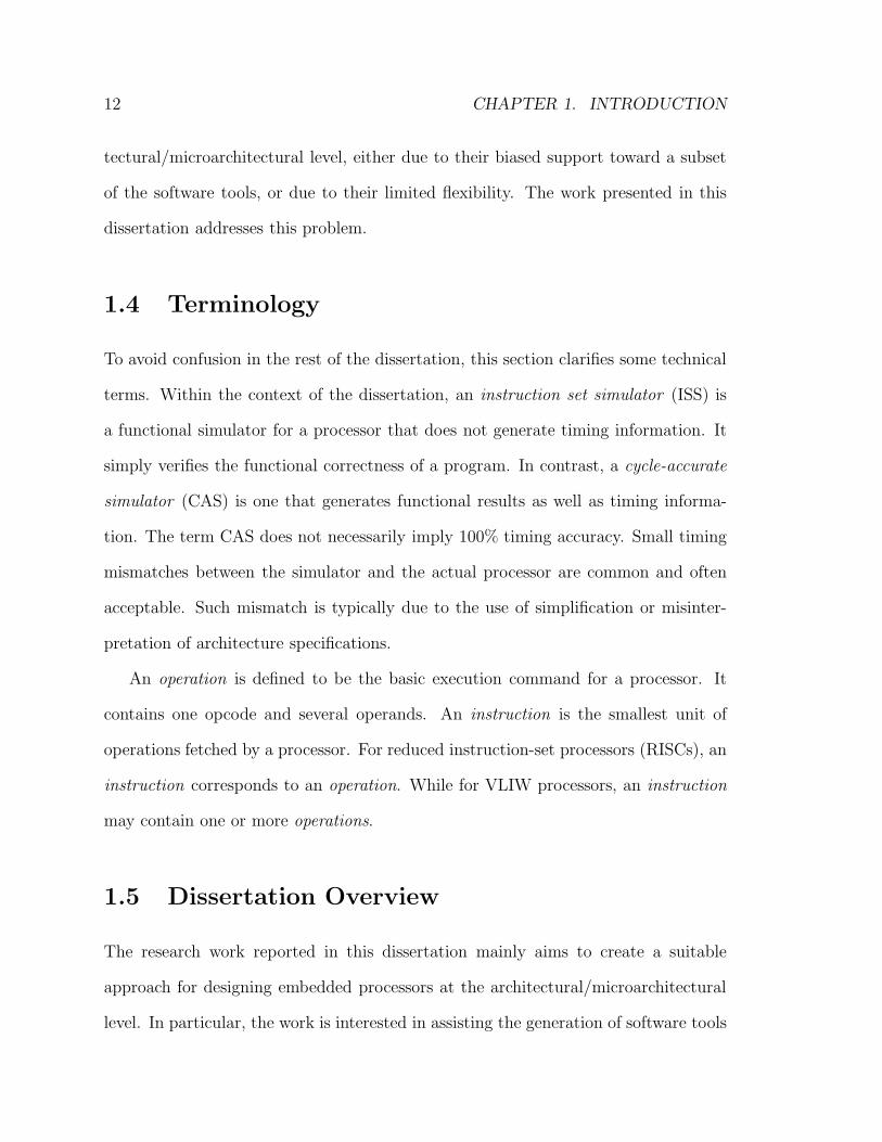
Besides the above mentioned issues, other issues plaguing nanometer design-
ers include signal integrity, electromagnetic interference, heterogeneous integration,
feature-limited yield, etc. Together with the increasingly complex system function-
ality, these issues have become serious challenges to chip designers. As a result, a
rising trend of design failures is observed. Figure 1.2 shows the number of spins
required to tape out a chip in year 2000 and 2002 [65, 61]. A spin means one itera-
tion between the design house and the fabrication facility. The figure shows that an
increasing number of design projects require multiple spins to be implemented cor-
rectly, which means that integrated circuit design is becoming more risky and costly.
Such high costs raise the break even volume – the threshold shipping volume beyond
which a design is profitable – of a chip design. If this trend continues, very soon
only those high value products with guaranteed high shipping volume can justify cus-
tomized chip implementations in state-of-the-art technologies. This trend is further
confirmed by a recent market survey, which showed that the number of design starts
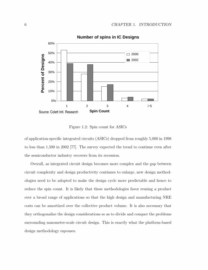
6 CHAPTER 1. INTRODUCTION
Number of spins in IC Designs
0%
10%
20%
30%
40%
50%
60%
1 2 3 4 �5
Spin Count
Per
cen
t o
f D
esig
ns 2000
2002
Source: Colett Intl. Research
Figure 1.2: Spin count for ASICs
of application-specific integrated circuits (ASICs) dropped from roughly 5,000 in 1998
to less than 1,500 in 2002 [77]. The survey expected the trend to continue even after
the semiconductor industry recovers from its recession.
Overall, as integrated circuit design becomes more complex and the gap between
circuit complexity and design productivity continues to enlarge, new design method-
ologies need to be adopted to make the design cycle more predictable and hence to
reduce the spin count. It is likely that these methodologies favor reusing a product
over a broad range of applications so that the high design and manufacturing NRE
costs can be amortized over the collective product volume. It is also necessary that
they orthogonalize the design considerations so as to divide and conquer the problems
surrounding nanometer-scale circuit design. This is exactly what the platform-based
design methodology espouses.
1.2. PLATFORM-BASED DESIGN 7
1.2 Platform-Based Design
The idea of platform-based design has long existed in the field of personal computer
designs. It was recently generalized by Sangiovanni-Vincentelli for use in electronic
system designs [93]. He defined a platform as “an abstraction layer in the design flow
that facilitates a number of possible refinements into a subsequent abstraction layer
in the design flow”. This definition extends the concept of platform to all design steps
from the system design level to the silicon implementation level.
In essence, a platform is an abstraction that separates design concerns into two
levels and thereby reduces the overall design complexity. For instance, the instruction
set architecture of a processor as a platform separates the software interface from the
microarchitecture implementation. This allows programmers to focus on the seman-
tics of the instructions without worrying about the details of the microarchitecture.
It also allows reusing software programs on different microarchitecture implementa-
tions of the same instruction set. However, in theory the use of a platform limits the
efficiency of the design since design optimizations are performed locally at individual
levels. Such potential loss of efficiency is a price to pay for the improved productiv-
ity, which may in return offset the efficiency loss as stronger optimizations may be
engaged at each level.
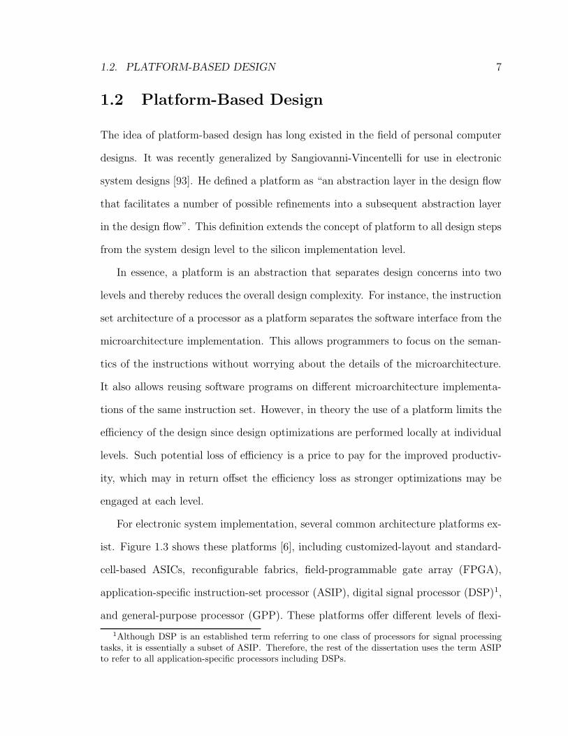
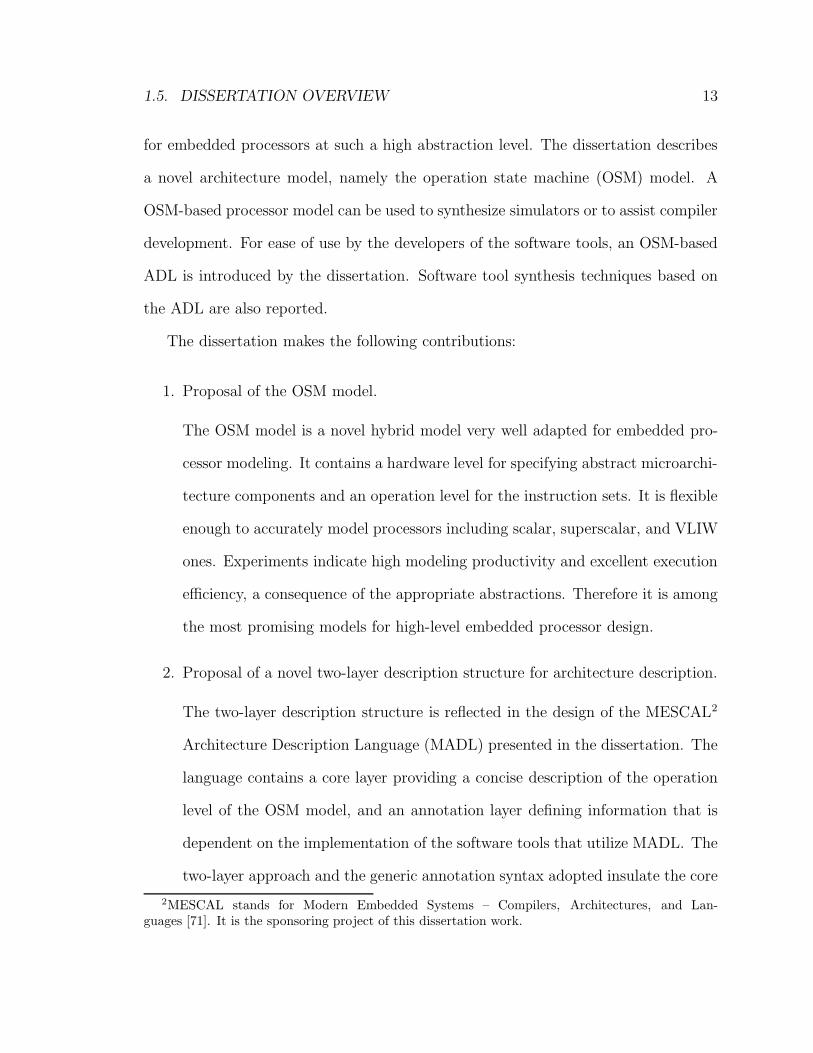
For electronic system implementation, several common architecture platforms ex-
ist. Figure 1.3 shows these platforms [6], including customized-layout and standard-
cell-based ASICs, reconfigurable fabrics, field-programmable gate array (FPGA),
application-specific instruction-set processor (ASIP), digital signal processor (DSP)1,
and general-purpose processor (GPP). These platforms offer different levels of flexi-
1Although DSP is an established term referring to one class of processors for signal processingtasks, it is essentially a subset of ASIP. Therefore, the rest of the dissertation uses the term ASIPto refer to all application-specific processors including DSPs.
8 CHAPTER 1. INTRODUCTION
ASIPASIP DSPDSPReconfReconf..FabricsFabrics
StructuredStructuredCustomCustom
RTLRTLFlowFlow
FPGAFPGA GPPGPP
Increased Flexibility
Increased P erf o rm ance, P o w er E f f iciency
Source: Gigascale Silicon Research Center
Figure 1.3: Common architecture platforms
bility and efficiency. On one end, the customized layout approach provides the best
performance and power efficiency but little flexibility. On the other end, a full soft-
ware solution based on GPPs provides great flexibility but possibly 10,000 times less
power and performance efficiency. All these platforms and their combinations provide
a rich set of options for designers to achieve a suitable trade-off between flexibility
and efficiency to meet their specific requirements.
1.3 Software Programmable Platforms
The past several years have witnessed a wave of network and communication SoC de-
signs that are based on architecture platforms with software programmability. Among
these, ASIPs are particularly favored by SoC designers because of their following ad-
vantages:
• ASIPs allow complex functionality to be implemented in software, which has
lower development costs than hardware-based solutions.
1.3. SOFTWARE PROGRAMMABLE PLATFORMS 9
• The flexibility of software makes it easy for the same product to cover multiple
related industrial standards and services. It also allows many design errors to be
quickly fixed in late development stages or even in the field, avoiding expensive
re-spins.
• ASIPs are customized with special architectural features targeting particular
families of applications. For those applications, ASIPs provide much better
performance and power efficiency than GPPs.
In summary, ASIPs feature a unique combination of productivity, flexibility, and
efficiency. They allow designers to implement complex functionality quickly, reducing
time to market. Their flexibility also enables easy extension of the system function-
ality to adapt to new market needs, lengthening product life time. These features are
very helpful for curbing the high design and manufacturing NRE costs of nanome-
ter systems. Therefore, the ASIP architecture platform is suitable to be used in
nanometer SoCs.
The growing popularity of the ASIPs encourages researchers to explore ASIP-
based SoC design methodologies. The generic system architectures favored by these
approaches are composed of multiple ASIPs, micro-controllers, hardware accelerators,
and on-chip communication networks. Such generic architectures are called software
programmable platforms. They have become important alternatives to ASICs for sys-
tem implementation, especially in network routing applications. The research work
presented in this dissertation focuses on the design automation of one component
of software programmable platforms – the processors, including ASIPs and micro-
controllers. Since these processors are implemented with better power and area effi-
ciency than GPPs, they are more suitable to be used in embedded SoCs. Therefore,
10 CHAPTER 1. INTRODUCTION
they are referred to as embedded processors in the rest of the dissertation. Although
the research results of the dissertation apply to GPPs as well, since their design styles
and their emphasis on performance are different from those of embedded processors,
they are not the main target of this work.
Modern embedded processors span a wide range of computer architecture fam-
ilies, including scalar, superscalar, very long instruction word (VLIW), and even
multi-threaded architectures. In contrast to GPPs, most of these processors have
relatively small shipping volumes (though together they constitute more than 90% of
total processors shipped [91]). As a result, they are usually designed by small teams
under tight budgets. In contrast to hardwired digital logic circuits, designers of these
processors need to deliver not only the hardware circuit implementation, but also the
software tools that help to utilize the programmability of the processors. As mature
commercial tool suites are available for circuit implementation, the development of
these software tools remains an art. The software tools include high-level language
compilers, assemblers, linkers, disassemblers, debuggers, and in some cases operat-
ing systems. For system development, the tools should also include instruction set
simulators and cycle-accurate simulators. These simulators help provide a virtual
prototype of the processors to both the circuit designers and the application soft-
ware developers. They also help verify system functionality and enable design space
optimization in the early design stages.
The software tools usually consist of tens of thousands of lines of source code in
C or C++. Some of the components, such as the simulators and compilers, are noto-
riously difficult to implement. Their developers need to have extensive training and
experience. Furthermore, due to the vast architecture scope of the embedded proces-
sors, there are no mature and flexible automation tools to help designers implement
1.3. SOFTWARE PROGRAMMABLE PLATFORMS 11
high quality software tools for all embedded processors. Therefore, the development
of the software tools constitutes a major challenge to the designers of the embedded
processors.
A common infrastructure used by software tool developers is the GNU software
tool chain, which is mainly developed by volunteers under the coordination of the Free
Software Foundation [87]. A GNU tool chain for a processor includes the high-level
language compiler(s), the assembler, the disassembler, the linker, and the debugger.
Experienced GNU programmers (a rare species) can retarget the tool chain to a new
processor by providing a mixture of machine description files, C macro definitions and
C code. This retargeting process usually yields reliable software tools. However, due
to the standard flow used in the GNU tool chain, it does not work well for irregular
instruction set architectures that are common to ASIPs. Moreover, the GNU tool
chain does not include simulator generation support. Therefore, it provides only a
partial solution to the problem.
In the past several years, a few startup companies, such as Tensilica [84] and
Improv [36], began to offer software programmable platforms and accompanying soft-
ware tools. Their tools have very limited reconfigurability based on the processor
templates adopted by the companies. Target Compiler Technologies [82] provides an
automated solution to synthesize compilers and simulators based on the nML archi-
tecture description language (ADL) [19]. Similarly, Axys [5] and Coware [15] pro-
vide simulator synthesis frameworks based on the LISA language [64]. Many other
ADL-based approaches have also been reported in academia. These approaches offer
different trade-offs between flexibility (in terms of architecture range), productivity,
and tool efficiency. As will be explained in Chapter 2 and Chapter 3, none of these
ADLs constitutes a satisfactory solution for embedded processor design at the archi-
12 CHAPTER 1. INTRODUCTION
tectural/microarchitectural level, either due to their biased support toward a subset
of the software tools, or due to their limited flexibility. The work presented in this
dissertation addresses this problem.
1.4 Terminology
To avoid confusion in the rest of the dissertation, this section clarifies some technical
terms. Within the context of the dissertation, an instruction set simulator (ISS) is
a functional simulator for a processor that does not generate timing information. It
simply verifies the functional correctness of a program. In contrast, a cycle-accurate
simulator (CAS) is one that generates functional results as well as timing informa-
tion. The term CAS does not necessarily imply 100% timing accuracy. Small timing
mismatches between the simulator and the actual processor are common and often
acceptable. Such mismatch is typically due to the use of simplification or misinter-
pretation of architecture specifications.
An operation is defined to be the basic execution command for a processor. It
contains one opcode and several operands. An instruction is the smallest unit of
operations fetched by a processor. For reduced instruction-set processors (RISCs), an
instruction corresponds to an operation. While for VLIW processors, an instruction
may contain one or more operations.
1.5 Dissertation Overview
The research work reported in this dissertation mainly aims to create a suitable
approach for designing embedded processors at the architectural/microarchitectural
level. In particular, the work is interested in assisting the generation of software tools
1.5. DISSERTATION OVERVIEW 13
for embedded processors at such a high abstraction level. The dissertation describes
a novel architecture model, namely the operation state machine (OSM) model. A
OSM-based processor model can be used to synthesize simulators or to assist compiler
development. For ease of use by the developers of the software tools, an OSM-based
ADL is introduced by the dissertation. Software tool synthesis techniques based on
the ADL are also reported.
The dissertation makes the following contributions:
1. Proposal of the OSM model.
The OSM model is a novel hybrid model very well adapted for embedded pro-
cessor modeling. It contains a hardware level for specifying abstract microarchi-
tecture components and an operation level for the instruction sets. It is flexible
enough to accurately model processors including scalar, superscalar, and VLIW
ones. Experiments indicate high modeling productivity and excellent execution
efficiency, a consequence of the appropriate abstractions. Therefore it is among
the most promising models for high-level embedded processor design.
2. Proposal of a novel two-layer description structure for architecture description.
The two-layer description structure is reflected in the design of the MESCAL2
Architecture Description Language (MADL) presented in the dissertation. The
language contains a core layer providing a concise description of the operation
level of the OSM model, and an annotation layer defining information that is
dependent on the implementation of the software tools that utilize MADL. The
two-layer approach and the generic annotation syntax adopted insulate the core
2MESCAL stands for Modern Embedded Systems – Compilers, Architectures, and Lan-guages [71]. It is the sponsoring project of this dissertation work.
14 CHAPTER 1. INTRODUCTION
layer from the frequent extensions of the software tools, lengthening the lifetime
of processor specifications in MADL.
The design of MADL also leads to the introduction of a dynamic version of
the OSM model, which is equally expressive as the originally OSM model. A
dynamic OSM model can be converted to the original model. In contrast to
the original model, the dynamic model integrates well with a syntax technique
named AND-OR graph used in MADL. The integration of the two in MADL
enables concise OSM description through factorization, making the use of the
OSM model practical.
To demonstrate the effectiveness of the MADL-based approach, a framework
for synthesizing CAS, ISS, and disassembler is implemented. The synthesized
CASs have been shown to have leading performance among the same class of
simulators. With the help of annotations, a tool to extract reservation tables
from MADL descriptions is also implemented. The reservation tables can be
used by a compiler component – the list instruction scheduler.
3. Proposal of a binary decoder synthesis algorithm supporting very fast instruc-
tion set simulation.
As a part of the CAS and ISS framework, a highly efficient binary decoder
synthesis algorithm is created and implemented. The algorithm takes simple
instruction encoding specification and generates very short binary decision tree
as the decoder. The generated decoders are shown to be more efficient than
its competitors. Due to the relatively small portion of time spent in decoding,
the algorithm does not significantly improve the efficiency of the CAS and ISS
1.5. DISSERTATION OVERVIEW 15
mentioned above. However, for cutting-edge hand-coded ISSs in which decoding
overhead is significant, the algorithm has greater impact.
The contributions of the dissertation are applicable to the design automation of
embedded processors. In particular, the OSM model is suitable to be used as the
semantic model for accurately specifying processors. Such a specification can then
be used to derive the software tools that are necessary to the development of the
processor. It can also be used to guide the logic implementation of the processor.
Thus, the proposal of the OSM model makes it possible to develop an integrated and
flexible design environment that targets both software and hardware development for
a wide range of embedded processors. MADL and the related software tool synthesis
framework reported in the dissertation are initial steps leading toward such a design
environment.
The rest of the dissertation is organized into the following chapters. Chapter 2
performs a comprehensive overview of related work in the field of architecture model-
ing and architecture description. It tabulates the main characteristics and usages of
the existing approaches for quick comparison. Then, Chapter 3 describes the OSM
architecture model and analyzes its advantages and limitations. It also compares
the OSM model to other related models. MADL is presented in Chapter 4. Two
important design considerations, the use of the AND-OR graph and the two-layer
approach, are described in detail. In Chapter 5, the synthesis of several software
tools is explained and experimental results are reported. The chapter also contains
a binary decoder synthesis algorithm that is suitable to be used for highly efficient
ISSs. Finally, Chapter 6 concludes the dissertation and points out future research
directions in the field.
Chapter 2
Related Work
2.1 Introduction
As per certain estimates [91], processors as a product family account for 30% of
the total revenue of all semiconductor circuits. Because of their enormous financial
importance, processors have become the research focus of many teams from both
academia and industry. The interests and expertise of these teams cover the broad
fields of computer architecture, logic design, electronic design automation, compiler
optimization, programming languages, formal verification, and more. As a result, the
emphases and approaches adopted by these teams vary greatly. The work reported in
this dissertation aims to assist the development of software programmable platforms
at the system level1. Therefore, it focuses on automating the design of embedded
processors through the generation of software tools such as simulators and high-level
language (HLL) compilers. This chapter provides an overview of the research efforts
with similar goals.
1This is in contrast to the logic implementation level.
16
2.1. INTRODUCTION 17
The development of processor-related software tools can be performed either man-
ually or automatically. On one hand, several teams feel most comfortable with the
general programming languages C and C++. They choose to develop these tools
manually in these languages. To improve development productivity, they have devel-
oped infrastructures that enhance the reusability of the manually written code. On
the other hand, many other research teams opted to develop frameworks that auto-
matically or semi-automatically generate the software tools. In these frameworks, a
processor specification is used to configure a retargetable software tool-chain or to
help synthesize a fully customized version of the tools for the target processor. In
such cases, the processor specification is usually called the architecture description,
and the description scheme is termed architecture description language (ADL).
Depending on the intent of the ADL, it may contain information representing
different views of a processor, such as the microarchitecture, the memory organization,
the instruction semantics, the assembly syntax, the instruction encodings, and the
abstract binary interface (ABI)2. According to the nature of the information provided,
ADLs are traditionally classified into three categories: structural ADLs, behavioral
ADLs, and mixed ADLs [90, 67]. Structural ADLs utilize component netlists to
describe the structural details of processors at the logic or the microarchitecture
level. They are suitable for synthesizing hardware and generating CASs. In contrast,
behavioral ADLs focus on describing the instruction set of the processor. They are
more suitable for generating compilers or ISSs. Mixed ADLs lie somewhere in between
and contain both instruction set and coarse-grained structural information.
The abstraction of the instruction set architecture (ISA) is one important char-
acteristic that distinguishes processors from general digital circuits. Therefore, most
2ABI defines the run-time interface between an application program and the operating system.
18 CHAPTER 2. RELATED WORK
existing ADLs take advantage of the abstraction and describe the instruction set
information explicitly. Among these ADLs, a majority contain some structural in-
formation such as the pipeline organization. As a result, a large number of ADLs
fall into the mixed category, making the traditional ADL classification method in-
effective. To avoid the problem, this chapter classifies the ADLs from a different
perspective – their architecture models. The architecture model refers to the model of
computation (MoC) used to represent the concurrency in the processor at both the
instruction set and the microarchitecture levels. It defines how the architectural or
microarchitectural components operate and how they interact with each other, which
is the key execution semantics of a processor. Therefore, this dissertation views the
architecture model as the most important factor that determines the quality of an
ADL. A classification method based on the architecture model helps to provide an
incisive understanding of the existing ADLs. It also helps evaluate the qualities of
the non-ADL approaches that are based on the general programming languages C or
C++.
2.2 Survey of Architecture Modeling Approaches
This section surveys various architecture models used for processor design, modeling,
and software tool development purposes.
2.2.1 Discrete Event Model
The discrete event (DE) model is the standard MoC for modeling digital circuits.
Common hardware description languages such as Verilog [35] or VHDL [34] all utilize
the DE model. In this model, a circuit is expressed as a list of modules connected
2.2. SURVEY OF ARCHITECTURE MODELING APPROACHES 19
through ports and channels. A module may be defined as sensitive to the signals at
some of its input ports. A signal is modeled as an event in the DE MoC. It carries a
time stamp indicating the moment when it needs to be activated. All pending events
are buffered in the global event calendar (also called event queue) according to the
chronological order. During the execution of the model, when system time advances,
the event calendar activates those events whose time stamps become current. It also
removes these events from the event buffer after their activation. Activating an event
triggers the modules that are sensitive to it. These modules may in turn generate
future events, which are to be buffered in the event calendar. The time stamps of the
new events are determined by the delay of the modules.
The DE MoC has been used by a few early ADLs and some recent modeling
approaches based on C++. MIMOLA is one of these ADLs [96]. It contains two
parts: the computer hardware description part and the high-level programming part.
The hardware description part is based on the DE MoC at the register transfer level
(RTL level), whose low hardware abstraction level requires that the updates of all
the hardware states (registers or memories) be explicitly scheduled by the model
developer. MIMOLA has been used by a series of tools including the MSSH hardware
synthesizer, the MSSQ code generator, the MSST self-test program compiler, the
MSSB functional simulator, and the MSSU RTL simulator [47].
Another DE-based processor description language is UDL/I developed at Kyushu
University in Japan [2]. It serves as the input to the COACH ASIP design automation
system. The COACH system can extract the instruction set from the RTL level
description in UDL/I for a small class of processors. The instruction set information
can be used to generate a target specific compiler and an ISS.
20 CHAPTER 2. RELATED WORK
HASE is a processor modeling environment based on the DE MoC [11]. Its mod-
ules are described in C++ as light-weight threads, which are scheduled by a DE
simulation engine. An entity description language (EDL) was developed to specify
the parameters and the interconnections of the modules. Compared to MIMOLA
and UDL/I, the components in HASE are of much coarser granularity. Therefore,
HASE provides better simulation efficiency and is more suitable to model sophisti-
cated processors such as GPPs. Similar to HASE, SystemC is a standard C++ library
supporting DE-based simulation [24]. It has also been used to model processors [53].
The DE MoC is most flexible since it is capable of modeling arbitrary logic circuits.
It is straightforward to synthesize cycle-accurate simulators from DE-based models.
For DE-based RTL level descriptions, hardware can be synthesized by commercially
available tools. However, the DE-based approaches have the significant drawbacks of
low abstraction level and low simulation speed. As a result of the low abstraction
level, it is hard to automatically extract instruction set information from the DE-
based structural specification for use in HLL compilers. To work around this problem,
the DE-based ADLs place constraints on the description style and the architecture
range for use in HLL compiler generation. In the case of MIMOLA, the MSSQ code
generator only works for the “micro-programmable controller” type of processors. In
other words, all control signals of the processor must originate from the instruction
word register [47]. MSSQ also requires that linkage information (hints) be specified
so that it can infer important information such as the location of the instruction word
register in the description. Similar architecture range and description style constraints
also exist for UDL/I.
2.2. SURVEY OF ARCHITECTURE MODELING APPROACHES 21
2.2.2 Synchronous Structural Models
Mainstream processors are implemented as synchronous logic circuits. Therefore, a
synchronous MoC is sufficient to model the vast majority of processors. Synchronous
MoCs do not need the expensive event calendar and therefore are more efficient
for use in simulators. This section discusses those modeling approaches that utilize
synchronous MoCs and describe processors from a structural stand-point.
Asim [18] is a processor modeling environment developed at Compaq for perfor-
mance modeling of high-end processors. Two types of modules exist in Asim, the
physical modules and the algorithm modules. The physical modules represent real
hardware components; while the algorithm modules represent the abstract operation
of the hardware, such as the cache replacement policy. The concept of the algorithm
module is introduced mainly for modularity and reusability concerns. In an Asim
model, the physical modules communicate with each other in a clock-driven fashion.
At each clock edge, all modules are activated simultaneously. Each module updates
its outputs according to its current states, its inputs, and its evaluation semantics.
Its updated output values can be used as the inputs of its neighboring modules in the
following cycle.
The clock-driven MoC of Asim is actually a special case of the DE MoC. In such
a model, the modules are only sensitive to the recurring clock signal. The limitation
of this specialized MoC is that combinational components such as the translation
look-aside buffer (TLB) cannot be defined as a standalone physical module. They
must be embedded into the models of other sequential components.
The Liberty Simulation Environment (LSE) [92] is based on a sophisticated syn-
chronous model, the Heterogeneous Synchronous/Reactive (HSR) MoC [17]. In an
HSR system, structural components are viewed as black boxes connected by unidi-
22 CHAPTER 2. RELATED WORK
rectional unbuffered channels. When the system receives any input, the components
connected to the input channel will react instantaneously according to their opera-
tional semantics and change their outputs. Such outputs will further trigger down-
stream components, which will in turn update their outputs instantaneously. The
process continues until all outputs stabilize. During the process, a component may
be repeatedly triggered if a cyclic dependency is present. Edwards showed that if
each component satisfies the monotonicity requirement [17], the system will always
converge.
The HSR model is well suited for control logic modeling. LSE exploits this feature
of HSR to ease the specification of operation flow control in processor pipelines.
Instead of creating dedicated hardware modules to control the execution progress
of the pipeline, LSE integrates a flow control protocol into the connectivity of the
pipeline stage modules. A stall in one stage of the pipeline can be propagated to
all upstream stages through the instantaneous HSR signaling mechanism. With this
scheme, no dedicated pipeline control logic is needed in LSE.
In LSE, HSR-based processor models are described in the Liberty Structural Spec-
ification (LSS) language. The language implements features such as polymorphic
module types and parametric scalability to improve module reusability and modeling
productivity.
The synchronous structural modeling approaches target the generation of CASs,
but not ISSs or HLL compilers. For the modeling of logic hardware, the synchronous
structural models are less flexible than DE models as they do not capture timing
details beyond the resolution of a clock period. Consequently, they cannot model
digital circuits such as a ring oscillator. However, such limitation does not translate to
significant drawbacks for processor modeling at the microarchitecture level. To most
2.2. SURVEY OF ARCHITECTURE MODELING APPROACHES 23
computer architects, their improved simulation efficiency over DE models overshadows
this limitation.
2.2.3 Synchronous Behavioral Model
The DE and synchronous structural models use component netlists to model hardware
structures. The communication between the modules is achieved through ports and
channels. During execution, a signal value is copied from the sending module to
the channel and then to the receiving module. Such indirection of communication
introduces significant runtime overhead in simulation.
UPFAST achieves faster simulation speed by avoiding using structural netlists [60].
In an UPFAST model, the communication between microarchitecture modules is
achieved through referencing the resource names, which are declared as globally ac-
cessible variables. For instance, reading a value from a register file is performed as
a reference to a global array variable. A pipeline stage’s internal states can also be
accessed in the same style.
Another important characteristic of UPFAST is the explicit specification of in-
struction behaviors. In contrast, netlist-based models embed instruction semantics
into the behavior of hardware modules, which causes difficulties in extracting instruc-
tions from those models.
For the ease of concurrency modeling, UPFAST breaks a clock cycle into several
artificial minor cycles. The behavior specification of an instruction is divided into a
number of time annotated procedures (TAP). Each TAP is labeled with a pipeline
stage name and a minor cycle index, representing where and when its behavior should
be evaluated. Suppose at a simulation cycle, instruction I arrives at a pipeline stage
24 CHAPTER 2. RELATED WORK
named P. The simulator will evaluate all TAPs of I that are labeled with P. The
evaluation order is in line with the minor cycle index of the TAPs.
The synchronous simulation scheme of UPFAST is straightforward to implement
and has very fast simulation speed. However, the modeling approach is not ele-
gant. First, it lacks modularity as hardware states are shared in the global context.
Although this brings about speedup in simulation, it affects reusability and creates
potential sources of software bugs. Second, it places a heavy burden on model develop-
ers who must sequentialize instruction behaviors into TAPs. In particular, designers
must create artificial minor cycles to ensure that dependent TAPs will be evaluated
in the right order. The complexity of scheduling all TAPs to minor cycles is similar
to that of the RTL level modeling. Such a simple concurrency modeling scheme offers
little productivity improvement compared with stylized C programming.
2.2.4 Abstract State Machine Model
BUILDABONG is a relatively young design environment for ASIP design [83]. It
models the hardware structures of processors based on the Abstract State Machine
formalism (ASM). An ASM model simply contains a set of transition rules in the
form of
if < cond > then < updates > .
At every cycle, all rules will be evaluated simultaneously. Each rule tests its Boolean
condition “cond”, and then evaluates the “updates” statements if the condition is
true. The rules represent the hardware implementation of the processor at the RTL
level.
The graphical front end of BUILDABONG translates the RTL level netlist of a
processor into an ASM specification, which can be simulated by generic ASM sim-
2.2. SURVEY OF ARCHITECTURE MODELING APPROACHES 25
ulators. The synchronous nature of the ASM model enables faster simulation speed
than in the DE case. Also, its low abstraction level allows for easy synthesis of logic
implementations. However, the low productivity of ASM specification at the RTL
level limits the use of BUILDABONG to simple ASIP designs.
2.2.5 Domain-specific Model
Most modern processors are pipelined. Pipeline stages are generally viewed by com-
puter architects as place holders or execution resources for instructions. This view
point is partially exploited by UPFAST in that it separates most instruction behav-
iors from the description of pipeline stages. It treats pipeline stages as the location
context for the evaluation of instruction behaviors. But pipeline stages still operate
as hardware modules in UPFAST. They perform tasks such as data forwarding.
A few ADLs are more aggressive in minimizing the role of the pipeline stages. In
these ADLs, the pipeline stages are pure place holders. Meanwhile, these ADLs treat
instructions as first class entities. Their description of instruction behaviors defines
the major functionality of a processor. Such instruction-centric scheme is typical in
behavioral and mixed ADLs.
LISA is an ADL developed at Aachen University of Technology in Germany [64]. It
has been commercialized by AXYS [5] and CoWare [15]. The atomic functional entity
in LISA is the operation3, which roughly corresponds to the behavior of an instruction
inside of a pipeline stage. The LISA simulation kernel utilizes the Gantt-Chart (equiv-
alent to the pipeline diagram) to control the execution progress of instructions. The
Gantt-Chart is a table representing the occupancy of pipeline stages over time. The
occupants of the pipeline stages are instructions. In an CAS generated from LISA,
3This is different from the operation defined in Section 1.4.
26 CHAPTER 2. RELATED WORK
each pipeline stage contains an operation buffer. When an instruction is fetched and
decoded, it is decomposed into several operations, which are inserted to the operation
buffers of the corresponding pipeline stages. An operation will be evaluated when its
parent instruction progresses to the pipeline stage.
The MoC adopted by LISA is the combination of the Gantt-Chart and its opera-
tion management mechanism. In essence, the concept of the LISA operation is similar
to the TAP in UPFAST. But the LISA model is of a higher abstraction level. It mod-
els most pipeline behaviors such as data forwarding through the use of operations. In
comparison, UPFAST specifies these behaviors inside the pipeline stages. Moreover,
while a TAP is simply a procedure, a LISA operation is more flexible in that it is
treated as a thread and can spawn other operations. Overall, the processor modeling
approach of LISA appears technically more interesting than that of UPFAST.
RADL is very similar to LISA since it is derived from an early version of LISA [76].
ArchC is a new ADL being developed in University of Campinas in Brazil [74]. It
also utilizes Gantt-Chart in its simulation engine. A special feature of ArchC is that
it is based upon SystemC. Except for several special syntax constructs, the main
part of an ArchC description is in C++. A preprocessor can translate the special
syntax constructs into SystemC implementations, which can integrate seamlessly with
the C++ part. This feature gives ArchC great flexibility to incorporate arbitrary
functionality allowed by SystemC. Since SystemC is based on DE, the MoC of ArchC
can be viewed as the combination of Gantt-Charts and DE.
In summary, the Gantt-Chart is a domain-specific model targeting processors
with in-order pipelines. Due to this limitation, ADLs such as LISA and RADL cannot
model superscalar processors with out-of-order issuing. ArchC could potentially work
around this limitation by falling back onto its SystemC foundation.
2.2. SURVEY OF ARCHITECTURE MODELING APPROACHES 27
2.2.6 Architecture Templates
Many ADLs were created as configuration systems for the software tools that they
intended to support. In a typical design environment based on such an ADL, a
generic processor template serves as the starting point of the description. The ADL
files provide parameters to configure some aspects of the processor template that
are of interest to the software tools. In this dissertation, such processor models are
classified as architecture templates. An architecture template supports the modeling
of a smaller processor range than the previously discussed models. This section
introduces several ADLs using architecture templates.
EXPRESSION is an ADL developed to assist the generation of both simulators
and HLL compilers [28]. It utilizes coarse-grained netlists (similar to sketch diagrams)
of pipeline stages and storage components to specify the structure of a processor.
Similar to the domain-specific models, EXPRESSION views pipeline stages as pure
place holders. Each stage is simply configured with several parameters including the
name of the output latch, the names of the ports, the capacity of the stage, the
operations that can go through the stage, and the latency.
In the early version of EXPRESSION [28], pipeline control information, such as
the conditions to stall and to flush, is implicit. Implicit pipeline control is common to
ADLs based on architecture templates as such control information is hard-coded into
the ADL as assumptions. The inability to customize pipeline control limits the range
of architectures that can be modeled. A later EXPRESSION paper [50] reported
a modeling scheme for a part of the pipeline control. The scheme is still template-
based and no detail was given on how such control specification is integrated into the
original EXPRESSION.
28 CHAPTER 2. RELATED WORK
PRMDL specifies processors in a style similar to EXPRESSION [85]. It serves as
a parametric system for configuring its retargetable compiler and simulator for a class
of clustered VLIW DSPs. PRMDL does not describe instruction semantics explicitly.
Instead, it specifies the mapping from compiler intermediate representation to actual
machine instructions.
The IMPACT research compiler infrastructure [3] utilizes the HMDES language [25]
to specify reservation tables to retarget its instruction scheduler. A reservation table
is a common data model representing simplified timing information of an instruction.
It abstracts structural components as discrete resources and describes the temporal
and spatial resource usage of the instruction. Based on such resource usage informa-
tion, the instruction scheduler can reorder the assembly code so as to reduce resource
conflicts and improve processor performance. HMDES utilizes the AND-OR graph
to compress the specification of the reservation tables. Details of the AND-OR graph
technique will be given in Section 2.3.2.
nML was originally developed to specify ISAs [19]. Therefore, it was categorized
as a behavioral ADL [90, 67]. It was later commercialized and extended to include
structural and timing information [82]. In its new version, instruction semantics can
be described with regard to the pipeline stages that it goes through. This reflects a
description scheme similar to LISA or ArchC. However, the specification of pipeline
control and timing information in the new nML is still largely based on parameters.
Due to this constraint, nML is mainly used to design DSPs with simple pipeline
control.
ISDL is a behavioral ADL for specifying ISAs of DSPs [26]. Limited instruction
timing information such as execution latency can be specified in ISDL. But no pipeline
control specification is supported. ISDL intends to assist the retargetable compila-

2.2. SURVEY OF ARCHITECTURE MODELING APPROACHES 29
tion and simulation of simple DSPs. It supports describing irregular instruction set
constraints with Boolean expression.
Similar to ISDL, TDL utilizes limited parameters to specify instruction timing
information [40]. It was used in a post-pass optimization (assembly optimization)
framework named PROPAN. It targets VLIW DSPs with simple control paths.
The Marion retargetable C compiler utilizes the Maril ADL to specify proces-
sors [8]. The target scope of Maril is GPPs with RISC style instruction sets. Its
instruction timing specification scheme is similar to that of ISDL and TDL. The
timing information is converted to reservation tables to be used by the retargetable
instruction scheduler of Marion. In comparison to DSPs, inaccuracy in timing spec-
ifications is more tolerable for GPPs. The reason is that GPPs have interlocking
mechanisms to enforce data dependency of the executing instruction stream, while
many DSPs fully rely on the compiler to handle data dependency through precise
instruction scheduling. As a matter of fact, it is hard to define exact instruction
latencies in a GPP pipeline since components such as caches or branch predictors can
make them less deterministic. Therefore, the timing information in Maril descriptions
is approximate.
The Tensilica Instruction Extension Language (TIE) [94] is a commercial descrip-
tion language for instruction extensions of Tensilica’s Xtensa processors. The base
microarchitecture and instruction set of each Xtensa processor are predefined by Ten-
silica. Users can augment the processor with new instructions that are created to
improve the execution efficiency for a particular set of applications. The binary en-
coding, assembly syntax, semantics, execution latency, and extra registers for the
new instructions can be described in the TIE language. The TIE compiler translates
the description to logic implementation for the new instructions as well as related
30 CHAPTER 2. RELATED WORK
additions to the software tools. As most features of the processors are already pre-
defined, the flexibility of TIE is rather limited compared to the other template-based
approaches. A similar commercial approach to Tensilica is adopted by Improv [36],
which allows users to configure its generic DSP templates.
The architecture template approaches are not based on well-defined concurrency
MoCs. One clear advantage of these ADLs is that the processor descriptions are
concise as much information is already embedded into the generic template. Another
advantage is that it is relatively easy to develop production quality software tools,
especially HLL compilers, based on the templates. The drawback of architecture tem-
plates, however, is their significantly limited architecture range. As the architecture
range can hardly be rigorously defined through formal mathematical means, it is dif-
ficult to convey such range limitation to general users of the ADLs. Therefore, most
of these ADLs remain for in-house use. The few commercial ones, such as TIE, are
restricted by very narrow templates and support very small architecture ranges.
2.2.7 Formal Mathematical Models
Mathews et al. designed a functional language named HAWK for describing processors
at the RTL level [49]. One potential advantage of a functional language is the ease of
verifying some processor properties. However, it is not intuitive for most computer
architects to specify hardware in such a language. The practicality of the approach
remains a question.
Hoe and Arvind proposed an operation-centric hardware description approach and
have used it to model processors [32]. The approach is based on the theory of Term
2.2. SURVEY OF ARCHITECTURE MODELING APPROACHES 31
Rewriting Systems (TRS). In TRS, hardware is modeled as a set of rules. Each rule
takes the form of
s′ = if π(s) then δ(s) else s.
During evaluation, if the condition π(s) for current state value s is true, then the
state value will be updated by δ(s). Otherwise the state value remains unchanged.
Although this rule appears similar to the ASM transition rule in BUILDABONG,
a significant difference is that rule update in TRS is non-deterministic. When more
than one TRS rule is enabled, the system randomly picks one of them to evaluate and
leaves the rest to future steps. In contrast, all ASM transition rules update simulta-
neously. Such non-deterministic behavior of TRS reflects a high-level asynchronous
model of processors. Hoe and Arvind developed a synthesis algorithm that transforms
the TRS rules into deterministic and synchronous hardware implementations. The
algorithm generates a finite state machine as the control logic that coordinates the
rule update sequence. The operation-centric technology was recently adopted by a
startup company named Bluespec [7].
Compared with traditional RTL level logic design methods, the operation-centric
approach allows designers to focus on the actual behavior of hardware components
rather than their timing and coordination, which implies a higher abstraction level in
design and may lead to higher productivity. It seems to be a promising behavioral level
design approach. However, for architecture modeling purposes, its abstraction level is
lower than those of domain-specific and template models. Hence the operation-centric
approach is not as productive in this regard.
Closely related to the TRS is the use of Petri-net variants to model processors [16,
98, 9]. Petri-net is a mathematical model for asynchronous and nondeterministic
concurrent system modeling. The Petri-net-based approaches model the structure

32 CHAPTER 2. RELATED WORK
of the processor hardware at various abstraction levels including the RTL level, the
behavioral level or even the transaction level. An introduction to Petri-nets will be
given in Chapter 3.
2.2.8 Other Work
CSDL is a family of machine description languages developed for the Zephyr com-
piler infrastructure [72]. It contains CCL, a function calling convention specification
language; SLED, a formalism describing instruction assembly syntax and binary en-
coding; and λ-RTL, a register transfer language for instruction semantics description.
These languages describe the instruction set and the programming interface of a pro-
cessor. SLED is also a part of the New Jersey Machine-Code Toolkit [73].
BABEL [51] is a recent ADL for retargeting the popular processor simulation
framework SimpleScalar [4]. Similar to CSDL, it describes the instruction set and the
programming interface of a processor. No detail was released on its microarchitecture
modeling and description approach. It is likely based on the register update unit
(RUU) template used in SimpleScalar.
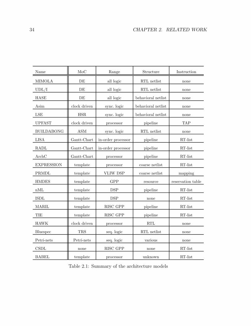
2.2.9 Summary of Architecture Models
As a summary of this survey, a list of the main characteristics of all the architecture
modeling approaches discussed above is given in Table 2.1. The columns of the table
stand for the name of the project, the architecture model, the architecture range
supported, the hardware structure description style and the instruction set description
style, respectively.
As shown in the table, the applicable architecture ranges of the models include
all logic circuits, sequential logic circuits, synchronous logic circuits, processors, and

2.2. SURVEY OF ARCHITECTURE MODELING APPROACHES 33
special families of processors. The structural description styles include component
netlist at the RTL level, component netlist at the behavioral level, coarse-grained
netlist, pipeline, and discrete resource. ISDL and CSDL contain no structural de-
scription. The hardware centric approaches do not support instruction set descrip-
tions. For most other approaches, instruction semantics are mainly specified in the
form of register transfer lists (RT-list), which are essentially statement lists defining
evaluation semantics. As exceptions, HMDES does not contain instruction seman-
tics description and PRMDL provides indirect semantics specification in the form of
mapping from intermediate representations to instructions. Though not shown in the
table, EXPRESSION also contains a similar mapping specification. In this sense,
EXPRESSION contains two parallel mechanisms for ISA specification.
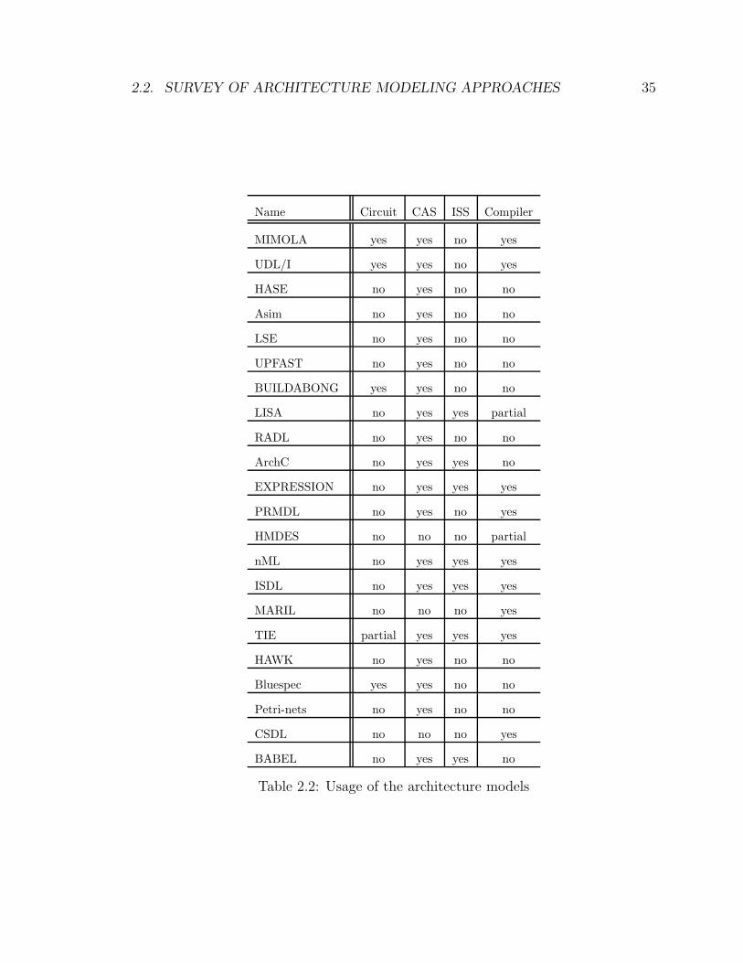
As mentioned earlier, the architecture modeling approaches were developed by
teams with different backgrounds and interests. Hence the approaches serve different
purposes. A summary of the main usage of these models is shown in Table 2.2. The
columns of the table represent the name of the project, support for logic synthesis,
support for CAS generation, support for ISS generation and support for HLL com-
piler generation, respectively. The entries in the table are based on actual published
results. Reported plans to support any of the tools are not taken into account. Since
LISA and HMDES only support the generation of the instruction scheduler, their
compiler support is deemed partial in the table. TIE supports synthesizing the logic
implementation of instruction extensions and therefore its circuit support is partial.
It is worth noting that the qualities of the modeling approaches and their related
software tools vary significantly. Since the implementation details of all projects are
not available, it is not possible to provide objective characterizations in this aspect.
34 CHAPTER 2. RELATED WORK
Name MoC Range Structure Instruction
MIMOLA DE all logic RTL netlist none
UDL/I DE all logic RTL netlist none
HASE DE all logic behavioral netlist none
Asim clock driven sync. logic behavioral netlist none
LSE HSR sync. logic behavioral netlist none
UPFAST clock driven processor pipeline TAP
BUILDABONG ASM sync. logic RTL netlist none
LISA Gantt-Chart in-order processor pipeline RT-list
RADL Gantt-Chart in-order processor pipeline RT-list
ArchC Gantt-Chart processor pipeline RT-list
EXPRESSION template processor coarse netlist RT-list
PRMDL template VLIW DSP coarse netlist mapping
HMDES template GPP resource reservation table
nML template DSP pipeline RT-list
ISDL template DSP none RT-list
MARIL template RISC GPP pipeline RT-list
TIE template RISC GPP pipeline RT-list
HAWK clock driven processor RTL none
Bluespec TRS seq. logic RTL netlist none
Petri-nets Petri-nets seq. logic various none
CSDL none RISC GPP none RT-list
BABEL template processor unknown RT-list
Table 2.1: Summary of the architecture models
2.2. SURVEY OF ARCHITECTURE MODELING APPROACHES 35
Name Circuit CAS ISS Compiler
MIMOLA yes yes no yes
UDL/I yes yes no yes
HASE no yes no no
Asim no yes no no
LSE no yes no no
UPFAST no yes no no
BUILDABONG yes yes no no
LISA no yes yes partial
RADL no yes no no
ArchC no yes yes no
EXPRESSION no yes yes yes
PRMDL no yes no yes
HMDES no no no partial
nML no yes yes yes
ISDL no yes yes yes
MARIL no no no yes
TIE partial yes yes yes
HAWK no yes no no
Bluespec yes yes no no
Petri-nets no yes no no
CSDL no no no yes
BABEL no yes yes no
Table 2.2: Usage of the architecture models
36 CHAPTER 2. RELATED WORK
2.3 Architecture Description Schemes
Processors are complex logic circuits. For the ISA specification alone, the program-
mer’s reference manual of a processor usually contains hundreds of pages. Therefore
it is a very time-consuming and error-prone process to develop processor models.
Consequently, modeling productivity has been one important concern of the projects
surveyed above. Productivity is mainly determined by the abstraction level of the
architecture model in use. It is also significantly affected by the description scheme
that presents the model. This section is an overview of the description techniques that
help to improve description productivity for hardware structures and for instruction
sets.
2.3.1 Structure Description Techniques
For processor structure descriptions, hierarchical component construction, and well
organized component libraries are common techniques to improve productivity. For
example, both HASE and LSE support hierarchical component construction with the
assistance of graphical user interfaces. HASE also formalizes the interfaces of the
library components so that only matching component interfaces can be connected.
Some ADLs have also explored syntactical techniques for describing structure in-
formation. For example, LSE experimented with the use of sophisticated techniques
such as polymorphic component types and automatic component type inference. The
techniques allow the definition of generic components that are capable of handling
data of different types. For example, a generic ALU for both integer and floating-point
computation can be defined. The actual type of an ALU instance is automatically
inferred according to the context of its use. If it is connected to integer data channels,
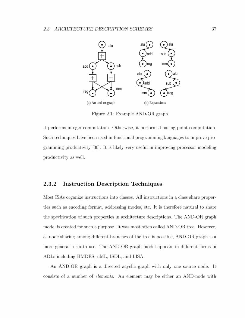
2.3. ARCHITECTURE DESCRIPTION SCHEMES 37
alu
add sub
regimm
alu
add
reg
alu
sub
imm
alu
add
imm
alu
sub
reg
(a) An and-or graph (b) Expansions
Figure 2.1: Example AND-OR graph
it performs integer computation. Otherwise, it performs floating-point computation.
Such techniques have been used in functional programming languages to improve pro-
gramming productivity [30]. It is likely very useful in improving processor modeling
productivity as well.
2.3.2 Instruction Description Techniques
Most ISAs organize instructions into classes. All instructions in a class share proper-
ties such as encoding format, addressing modes, etc. It is therefore natural to share
the specification of such properties in architecture descriptions. The AND-OR graph
model is created for such a purpose. It was most often called AND-OR tree. However,
as node sharing among different branches of the tree is possible, AND-OR graph is a
more general term to use. The AND-OR graph model appears in different forms in
ADLs including HMDES, nML, ISDL, and LISA.
An AND-OR graph is a directed acyclic graph with only one source node. It
consists of a number of elements. An element may be either an AND-node with
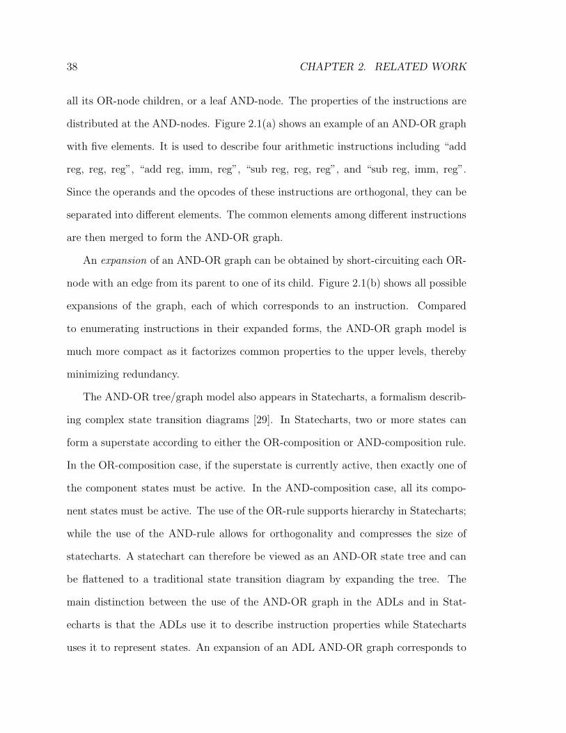
38 CHAPTER 2. RELATED WORK
all its OR-node children, or a leaf AND-node. The properties of the instructions are
distributed at the AND-nodes. Figure 2.1(a) shows an example of an AND-OR graph
with five elements. It is used to describe four arithmetic instructions including “add
reg, reg, reg”, “add reg, imm, reg”, “sub reg, reg, reg”, and “sub reg, imm, reg”.
Since the operands and the opcodes of these instructions are orthogonal, they can be
separated into different elements. The common elements among different instructions
are then merged to form the AND-OR graph.
An expansion of an AND-OR graph can be obtained by short-circuiting each OR-
node with an edge from its parent to one of its child. Figure 2.1(b) shows all possible
expansions of the graph, each of which corresponds to an instruction. Compared
to enumerating instructions in their expanded forms, the AND-OR graph model is
much more compact as it factorizes common properties to the upper levels, thereby
minimizing redundancy.
The AND-OR tree/graph model also appears in Statecharts, a formalism describ-
ing complex state transition diagrams [29]. In Statecharts, two or more states can
form a superstate according to either the OR-composition or AND-composition rule.
In the OR-composition case, if the superstate is currently active, then exactly one of
the component states must be active. In the AND-composition case, all its compo-
nent states must be active. The use of the OR-rule supports hierarchy in Statecharts;
while the use of the AND-rule allows for orthogonality and compresses the size of
statecharts. A statechart can therefore be viewed as an AND-OR state tree and can
be flattened to a traditional state transition diagram by expanding the tree. The
main distinction between the use of the AND-OR graph in the ADLs and in Stat-
echarts is that the ADLs use it to describe instruction properties while Statecharts
uses it to represent states. An expansion of an ADL AND-OR graph corresponds to
2.4. SUMMARY 39
the properties of an instruction while an expansion of an Statecharts AND-OR graph
corresponds to a state in the flattened state transition diagram.
Another interesting issue in instruction description for ASIPs is the handling of
irregular constraints. As ASIP designs are cost-sensitive, they often have irregular
constraints in their ISAs. Clustered or special-purpose register files with incomplete
data transfer paths are sometimes used to conserve chip area and power. Irregular
instruction word encoding has also been used as a means to save instruction word size,
and therefore the size of the instruction memory. An example irregular constraint
is the limited combinations between different operands for some operations of the
Fujitsu Hiperion processor [22]. In this case, the choice of a register for one operand
may be dependent on the choice for another operand.
Most ADLs that support instruction set description do not handle the irregular
constraints directly. For the above mentioned example, enumerating all possible com-
binations is the standard solution. However, a few ADLs, such as ISDL and TDL,
provide special syntax constructs to specify such constraints more effectively. They
use Boolean expressions to model such constraints. Compared with enumeration,
Boolean expressions or regular expressions are more concise for most constraints.
2.4 Summary
This chapter surveyed the previous research efforts in the field of processor model-
ing and description. It classified these research works according to the architecture
model used to represent the concurrency in processors. The existing architecture
models mainly include the discrete event (DE) model used by MIMOLA, UDL/I, and
HASE, the clock-driven model used by Asim, the heterogeneous synchronous/reactive
40 CHAPTER 2. RELATED WORK
(HSR) model adopted by LSE, the synchronous behavioral model of UPFAST, the
abstract state machine (ASM) model used by BUILDABONG, the Gantt-Chart used
by LISA, RADL, and ArchC, the term-rewriting systems (TRS) adopted by Bluespec,
and various architecture templates used by EXPRESSION, PRMDL, HMDES, nML,
ISDL, TDL, and Marion.
Depending on the emphasis of an architecture model in representing structural or
behavioral information, its usage varies. The structural models, including the DE,
clock-driven, HSR, ASM, and TRS models focus on hardware structures and therefore
are suitable to be used for the synthesis of hardware and CASs. While the Gantt-
Chart, the synchronous behavioral model and most architecture templates contain
both high-level structural and instruction set information. Therefore, they may be
used to generate cycle-accurate simulators, instruction set simulators, and compiler
components. The following chapter will further analyze these models regarding their
suitability to be used for the design of embedded processors.
This chapter also briefly surveyed processor description elements that help to im-
prove description efficiency. They include hierarchical structural composition, compo-
nent library, polymorphic component type, AND-OR graph and Boolean expression.

Chapter 3
Architecture Model
3.1 Introduction
As mentioned in Chapter 1, the focus of the dissertation work is the automation
tools and algorithms for the design of embedded processors to be used in software
programmable platforms. Figure 3.1 shows the standard design process of embed-
ded processors at the system level. The input to the process is a family of software
applications such as network routing or multimedia signal processing. The designers
first study the characteristics of the applications and propose a tentative platform
design expressed in the form of a system level architecture description. The descrip-
tion is used to configure the HLL compiler that translates the application source code
into binary machine code. The complete compilation process involves analyzing the
concurrency in the application, binding and scheduling tasks onto individual proces-
sors, and generating machine code for all processors. The architecture description is
also used to generate a system level cycle-accurate simulator (CAS) as the virtual
prototype of the platform. The CAS evaluates the performance of the tentative sys-
41
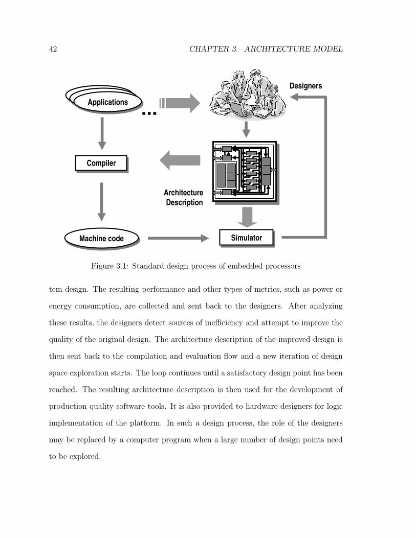
42 CHAPTER 3. ARCHITECTURE MODEL
Compiler Compiler
Simulator Simulator Machine codeMachine code
Architecture Description
DesignersApplicationsApplicationsApplicationsApplications
ApplicationsApplications
Figure 3.1: Standard design process of embedded processors
tem design. The resulting performance and other types of metrics, such as power or
energy consumption, are collected and sent back to the designers. After analyzing
these results, the designers detect sources of inefficiency and attempt to improve the
quality of the original design. The architecture description of the improved design is
then sent back to the compilation and evaluation flow and a new iteration of design
space exploration starts. The loop continues until a satisfactory design point has been
reached. The resulting architecture description is then used for the development of
production quality software tools. It is also provided to hardware designers for logic
implementation of the platform. In such a design process, the role of the designers
may be replaced by a computer program when a large number of design points need
to be explored.
3.1. INTRODUCTION 43
A critical component in the design flow of Figure 3.1 is the architecture description.
It records the design point in each iteration and serves as the interface between the
designers and the software tools. Therefore the description scheme directly affects
the quality of the design process and the final product. To ensure the quality of the
product, the description scheme must be effective in accurately reflecting the relevant
details of the design at a proper level of abstraction. It must also be effective in
supplying necessary information to the compiler and the simulator.
As has been pointed out in Chapter 2, the key determining factor for the quality of
a description scheme is the architecture model used by the description. To evaluate
the quality of an architecture model for use in the design flow of Figure 3.1, the
dissertation proposes to analyze the following four properties:
Compactness – Processors are complex hardware and it is a laborious process to
develop a processor model. To reduce the development effort, the architec-
ture model should be sufficiently compact so that designers can capture their
thoughts productively.
Flexibility – A larger design space provides more room for optimization. Therefore,
support for a broader architecture range by the architecture model potentially
leads to better designs. Moreover, the architecture model should be versatile
enough to reflect important characteristics of the target architectures faithfully
so as to minimize errors in the evaluation process.
Efficiency – The simulation of average real-world benchmarks typically takes from
tens of hours to weeks. It often becomes a bottleneck in the design space ex-
44 CHAPTER 3. ARCHITECTURE MODEL
ploration process.1 The simulation speed is directly affected by the architecture
model used, in particular, its abstraction level. Therefore, the architecture
model should have the potential to support efficient simulation so as to reduce
the design time.
Analyzability – The compiler needs to extract and analyze high-level architecture
properties such as the instruction semantics of the PEs for code generation.
A rule-based declarative model can more easily expose such properties than
imperative-style models.
In reality, these properties are often conflicting with each other. For instance, a
compact model requires a high abstraction level. However, a higher abstraction level
most likely implies reduced flexibility since it omits more implementation details,
some of which may be relevant to system level design. It is a very challenging task
to find the right architecture model that is well balanced in all these aspects.
The major contribution of the dissertation is the proposal of an architecture model
that is well positioned with respect to the above four properties. Therefore it is
suitable for use in the design flow for embedded processors at the system level. The
rest of the chapter introduces the model.
3.2 Problem Definition: Modeling Concurrency
Although processors are diverse in their computation power and their underlying mi-
croarchitectures, they share some common properties inherited from their ancestor –
1Statistical sampling techniques [13, 31, 95] have been used to reduce simulation time by measur-ing only chosen sections of the full simulation trace. Such techniques works well for the simulationof standalone programs. But in general they are not applicable to system-level simulation whereprograms react to the environment.
3.2. PROBLEM DEFINITION: MODELING CONCURRENCY 45
the von Neumann computer. They fetch instruction streams from memories, decode
operations, read register and memory states, evaluate operations per their semantics,
and then update register and memory states. Such software programmability at the
operation level is represented by the instruction set architecture (ISA) of a processor,
which is the main distinction between a processor and other types of logic circuits.
Thus, to represent processors effectively, an architecture model should explicitly pre-
serve the notion of instruction or operation so as to capture the ISA as an essential
characteristic of a processor. An explicit operation level specification also simplifies
the task of extracting architecture properties of the processor as is required by the
analyzability property.
Modern processors are often implemented with a high degree of parallelism. At
the least, most processors are pipelined. More than one operation can execute simul-
taneously at the different stages of a pipeline. Such overlapping of operation execution
latencies reflects the temporal parallelism in a processor. This parallelism is extended
in VLIW processors and superscalar processors, which are capable of fetching and is-
suing multiple operations at a time. This type of concurrency is a result of resource
duplication and reflects the spatial parallelism of a processor. The temporally and
spatially parallel operations interact with one another during their execution. Their
dynamic relationships, including resource contention, data dependency, and control
dependency, partially define the execution timing of a processor. Therefore, it is nec-
essary for the architecture model to precisely capture such interactions as is required
by the flexibility property.
From a hardware perspective, processors are still logic circuits. Many hardware
implementation details such as the number of physical registers or the size of the
cache are not visible to the ISA in most cases. For accurate modeling purposes, it is
46 CHAPTER 3. ARCHITECTURE MODEL
necessary to include these relevant details of the structural components in the proces-
sor model. Given the high structural complexity of average processors, an abstraction
level higher than RTL is necessary in order to meet the compactness and efficiency re-
quirements. The microarchitecture is a suitable abstraction level for structural mod-
eling as it is most familiar to computer architects. At the microarchitecture level,
basic building blocks include pipeline stages, reservation stations, caches, branch pre-
dictors, etc. The concurrent operation of these components is another determining
factor of the execution timing of a processor. Therefore, preserving the cycle-accurate
semantics of these components and their interactions is necessary to satisfy the flexi-
bility property. Furthermore, since operations are executed in the microarchitectural
components, it is also necessary for the architecture model to include the interaction
between the operations and the microarchitecture components.
In conclusion, an effective architecture model should contain information at both
the operation and the microarchitecture levels. To model the underlying concurrent
behaviors at and across the two levels, designers need to answer the following three
key questions:
1. How to represent the operations and their interactions in the operation level?
2. How to represent the microarchitectural components and their interactions in
the hardware level?
3. How to represent the interactions between the operations and the microarchi-
tectural components?
The survey of Chapter 2 indicates that it is hard to find an architecture model
that satisfactorily answers the above three questions and simultaneously preserves
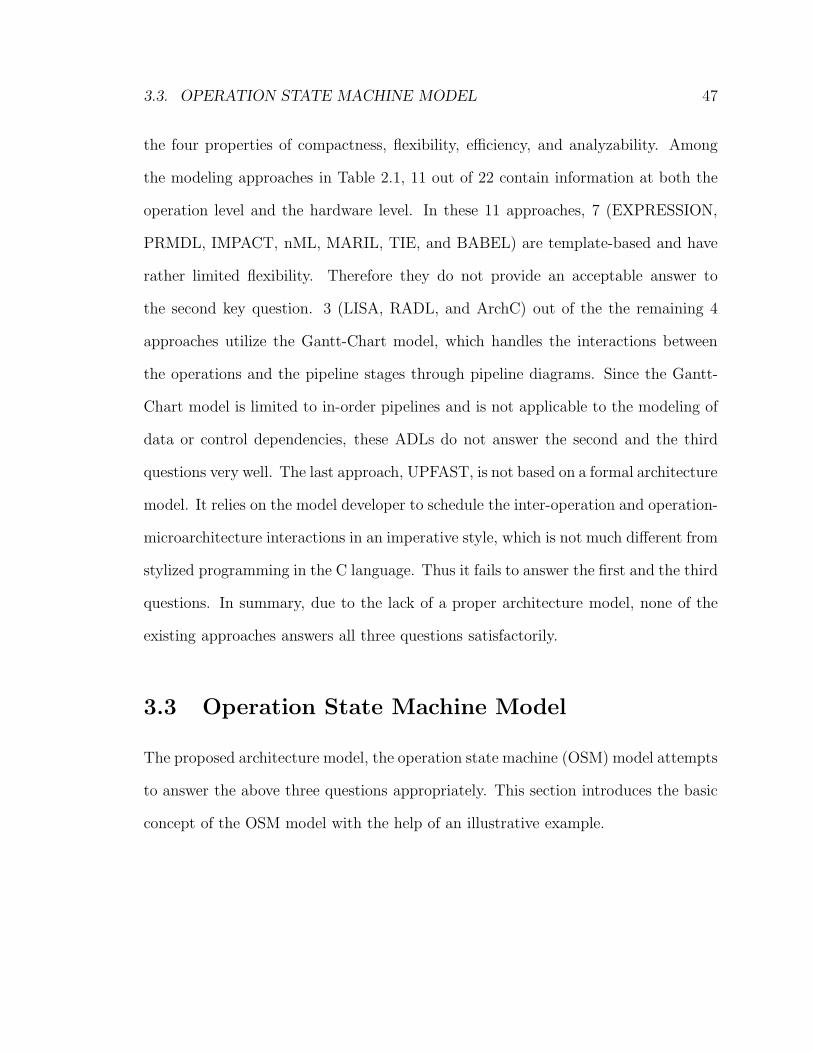
3.3. OPERATION STATE MACHINE MODEL 47
the four properties of compactness, flexibility, efficiency, and analyzability. Among
the modeling approaches in Table 2.1, 11 out of 22 contain information at both the
operation level and the hardware level. In these 11 approaches, 7 (EXPRESSION,
PRMDL, IMPACT, nML, MARIL, TIE, and BABEL) are template-based and have
rather limited flexibility. Therefore they do not provide an acceptable answer to
the second key question. 3 (LISA, RADL, and ArchC) out of the the remaining 4
approaches utilize the Gantt-Chart model, which handles the interactions between
the operations and the pipeline stages through pipeline diagrams. Since the Gantt-
Chart model is limited to in-order pipelines and is not applicable to the modeling of
data or control dependencies, these ADLs do not answer the second and the third
questions very well. The last approach, UPFAST, is not based on a formal architecture
model. It relies on the model developer to schedule the inter-operation and operation-
microarchitecture interactions in an imperative style, which is not much different from
stylized programming in the C language. Thus it fails to answer the first and the third
questions. In summary, due to the lack of a proper architecture model, none of the
existing approaches answers all three questions satisfactorily.
3.3 Operation State Machine Model
The proposed architecture model, the operation state machine (OSM) model attempts
to answer the above three questions appropriately. This section introduces the basic
concept of the OSM model with the help of an illustrative example.
48 CHAPTER 3. ARCHITECTURE MODEL
3.3.1 Abstractions
The OSM model views processors at two levels, the operation level and the hardware
level. The operation level contains the ISA and the dynamic execution behavior of the
operations. The hardware level represents the greatly simplified microarchitecture as
a result of the proper abstraction mechanisms used in the OSM model.
At the operation level, extended finite state machines (EFSM) are used to model
the execution of operations. An EFSM is a traditional finite state machine (FSM)
with internal state variables [10]. It can be transformed to a traditional FSM by
dividing each of its states into n states, where n is the size of the state space defined
by the internal state variables. The use of these state variables compresses the state
diagram and hides less relevant details of the state machine from its external view.
In an OSM-based processor model, one EFSM represents one operation, thus the
name operation state machine (OSM) is used for these special-purpose EFSMs. The
states of an OSM stand for the execution statuses of the operation that it represents;
while its edges stand for the valid execution steps. The states and the edges form the
state diagram of the OSM, which must be a strongly connected graph so that there
exists no dead-end state or isolated subcomponent2. The internal state variables of
the EFSM are used to hold intermediate computation results of the operation. To
control the state transition of the OSM, each edge of the OSM is associated with
a condition, which represents the readiness of the operation to progress along the
edge. Such readiness is expressed as the availability of execution resources, including
structural resources, data resources and artificial resources created for the purpose of
modeling. Example resources include pipeline stages, reorder-buffer entries and the
availability of operands.
2This is a requirement of the OSM model, not the EFSM.
3.3. OPERATION STATE MACHINE MODEL 49
R
WED
Ie0
e2e1
e3 e4
e5
src1, src2 available?function unit available?
reorder-buffer available?
src1, src2 available?function unit available?
reorder-buffer available?
src1, src2 available?function unit available?
reorder-buffer available?
src1, src2 available?function unit available?
reorder-buffer available?
reservation station available?reservation station available?
F
e6
fetching decoding
in reservation station
executing writing back
dormant
Figure 3.2: Example OSM for an out-of-order processor
Figure 3.2 shows an example OSM that models an operation in an out-of-order
processor. It contains 6 states representing the execution statuses as dormant, fetch-
ing, decoding, in reservation station, executing, and writing back, respectively. The
double-circled dormant state refers to the status when the operation is not in the pro-
cessor pipeline, either because it is not fetched yet or it has retired. Each OSM has
one and only one dormant state. The call-out boxes in Figure 3.2 show the conditions
on some of the edges. They test the availability of various execution resources.
The execution resources are maintained in the hardware level of the OSM model.
They are modeled as tokens. A token may optionally contain a data value. A token
manager controls a number of tokens of the same type. It assigns the tokens to the
OSMs according to its token management policy and the requests from the OSMs.
In essence, a token manager is an abstract implementation of a control policy in the
processor.
In the example of Figure 3.2, the function unit, the reorder-buffer entry, the reser-
vation station entry, and the source operands can all be modeled as tokens. Depending
50 CHAPTER 3. ARCHITECTURE MODEL
on the control semantics of the microarchitecture components, token managers with
different policies can be implemented. For instance, a function unit may be an ex-
clusive resource, viz., it is not sharable among operations. A corresponding token
manager with only one token can be implemented to control the usage of the function
unit by operations. The manager needs a single-bit flag to memorize the usage of the
token. The token can be assigned to an operation only if the flag indicates that it
is not in use. Similarly, a reorder-buffer token manager can also be implemented to
manage the tokens corresponding to its entries. Since a reorder-buffer can be viewed
as a queue with flushing capability [62], the matching data structure and algorithm
can be used to implement its control policy.
3.3.2 OSM Model
With the assistance of the two types of abstraction, the OSM model answers the three
key questions as follows.
1. How to represent the operations and their interactions in the operation level?
The operation level of the OSM model specifies the semantics and the dynamic
execution behavior of the operations. Its run-time model consists of a number
of OSMs. An OSM can be either in the active or the dormant status. In
execution, it repeatedly switches back and forth between the two as its state
progresses. In its active status, an OSM models one operation executing in
the processor. Its life range (from the time it becomes active to when it goes
back to dormancy) corresponds to that of the operation in the pipeline. In its
dormant status, the OSM awaits the opportunity to represent a new operation.
At each cycle, a few dormant OSMs may become activated as new operations are
3.3. OPERATION STATE MACHINE MODEL 51
fetched into the processor; and several active OSMs may go back to dormancy
as their corresponding operations retire from the processor. All OSMs execute
concurrently under the coordination of a synchronous OSM scheduler, which
ensures that they behave in a deterministic manner. The minimum interval
period between two state transitions for an OSM is called the control step of
the scheduler. Depending on the requirement for timing resolution, a control
step may be either a clock cycle or a clock phase. The OSMs do not directly
communicate with one another.
2. How to represent the microarchitectural components and their interactions in
the hardware level?
The microarchitectural components are modeled at the behavioral abstraction
level in general. They communicate with one another under the DE MoC. A
component may contain a token manager, which is an abstraction of a part
of the component’s behavior. The token manager shares states with the owner
component. It cannot directly communicate with microarchitecture components
other than its owner or other token managers But it can communicate with the
OSMs at the operation level. The details of such communication are provided
below in the answer to the third question. In the simplest case when it does not
need to communicate with other components, a microarchitecture component
is reduced to a pure token manager.
3. How to represent the interactions between the operations and the microarchi-
tectural components?
The only means for an OSM to communicate with the environment is to in-
teract with the token managers in the hardware level. A set of communication
52 CHAPTER 3. ARCHITECTURE MODEL
primitives are defined as the protocol for such interaction. The communication
primitives are called actions. An action always occurs between an OSM and a
token manager. It consists of three steps: first, the OSM sends a request to the
token manager; second, the token manager replies; and finally, if the response
from the token manager is positive, the OSM may choose to commit the action
or to abort the action. Otherwise, the action is aborted.
An action may belong to one of the two classes, control action and data action.
Control actions model resource transactions. They fall into the following four
categories.
Allocate – An OSM may request the ownership of a token from a token man-
ager. If the token is available to the OSM, the request succeeds and the
token manager can grant the ownership of the token to the OSM. This ac-
tion is used to model the transaction of exclusive resources. Most structure
resources in a processor are exclusive.
Inquire – An OSM may inquire about the status of a token without the inten-
tion to obtain it. The request succeeds if the token is available for access
to the OSM. This type of action is used for non-exclusive resource access.
One example of non-exclusive resource access is to test the availability of
a source operand.
Release – An OSM may release a token that has been allocated to it. The
token manager can either accept or reject the request.
Discard – An OSM may discard a token that it owns. The request is uncon-
ditional and always succeeds.
3.3. OPERATION STATE MACHINE MODEL 53
Once a token has been allocated to an OSM, it cannot be allocated to another
one until the first OSM releases or discards the token. But other OSMs may
still be able to inquire about the allocated token, depending on the policy of the
token manager. The discard action may be viewed as an unconditional version
of release. It is useful to model the resetting of an OSM in which case the
OSM gives up all the resources that it owns and goes back to the dormant state
directly.
The data actions include read and write. They allow an OSM to exchange data
values with its environment. As mentioned previously, some tokens may contain
a data value. An OSM can request to read the data value of such a token and
can store the value in an internal state variable. The request will succeed if the
OSM owns the token or it is able to inquire about the token. An OSM can also
request to write the value of an internal state variable to a token. The write
request can only succeed if the OSM owns the token.
One or more actions can be associated with each edge of an OSM. When an
edge is evaluated for state transition readiness at a control step, the requests
of its associated actions are sent simultaneously to the corresponding token
managers. Only if all requests succeed is the edge considered ready for a state
transition. All the actions must commit when the OSM transitions its state
along the edge. However, if any one of the requests fails, the edge is not yet
ready for a state transition and all actions abort. In summary, the condition
for a state transition along one edge is the conjunction of the responses of the
token managers to the actions on the edge.

54 CHAPTER 3. ARCHITECTURE MODEL
D Ee1
e21
e22
Allocate TM2, …Allocate TM2, …
Allocate TM1, …Allocate TM1, …
F
e31
e32
Release TM2, …Release TM2, …
Release TM1, …Release TM1, …
e4
Figure 3.3: An illegal OSM portion
It is often necessary for an OSM to point out the token that it is interested in
for an action. This is done by sending a token identifier along with the action
request. In general, the token identifier can be either an integer or a tuple of
two or more integers. The data type of the token identifier is a static property
of a token manager as it recognizes only one type of identifier for all its actions.
Some token managers do not need identifiers. For instance, if a token manager
controls only one token, there is no choice left for the OSMs. In such a case,
the token identifier is deemed as having a void type.
At its dormant state, an OSM owns no token. When it progresses along a path
in the state diagram, the allocate actions obtain tokens while the release and
discard actions do the reverse. It is possible to statically analyze the actions
along the path to know the number of tokens that the OSM owns at each state
and the types of the tokens (type here means the name of the token manager for
a token). As multiple paths from the dormant state may converge at the same
state, they may result in different set of token types at the state. For validity
checking and model analysis purposes, it is required that the set of token types
3.3. OPERATION STATE MACHINE MODEL 55
for a state be deterministic. In other words, regardless of the execution path
that leads to a state, the set of token types should be the same for the state.
According to this requirement, the state diagram portion in Figure 3.3 cannot
be from a valid OSM as at state E, the OSM may either own a TM1 token
if it came along e21 or a TM2 token if it came along e22. In this example,
the state E needs to be split into two states to become valid. This validity
requirement eliminates the potential erroneous situation when a transition along
e21 is followed by another along e32 in Figure 3.3. In such a case, the release of
of the TM2 token on e32 is illegal since the OSM does not own it at state E.
For the validity requirement to hold for the dormant state, an OSM should not
own any token when it returns to the dormant state.
It should be noted that the term action used here is different from that of the
Statecharts model [29] or its UML state machine variant [59]. In a statechart, a
transition (edge) is associated with an event, a guard condition and several “actions”.
If the source state of the transition is active, and if the event occurs, the guard
condition will be evaluated. If the condition is true, the “actions” will be fired and
the state transfers along the edge. An event in Statecharts is an observable occurrence
in the environment or in the statechart itself. It is a uni-directional communication
mechanism from the producer of the event to its consumer, which is different from
the OSM actions as they implement a bi-directional negotiation mechanism between
an OSM and the environment (the token managers). Therefore, the event has no
corresponding notion in the OSM model. The conjunction of the requests of the
OSM actions on an edge actually corresponds to a guard condition of Statecharts and
the committing of the OSM actions corresponds to Statecharts “actions”. Although
it is possible to express OSMs with Statecharts notations in principle, it is not very
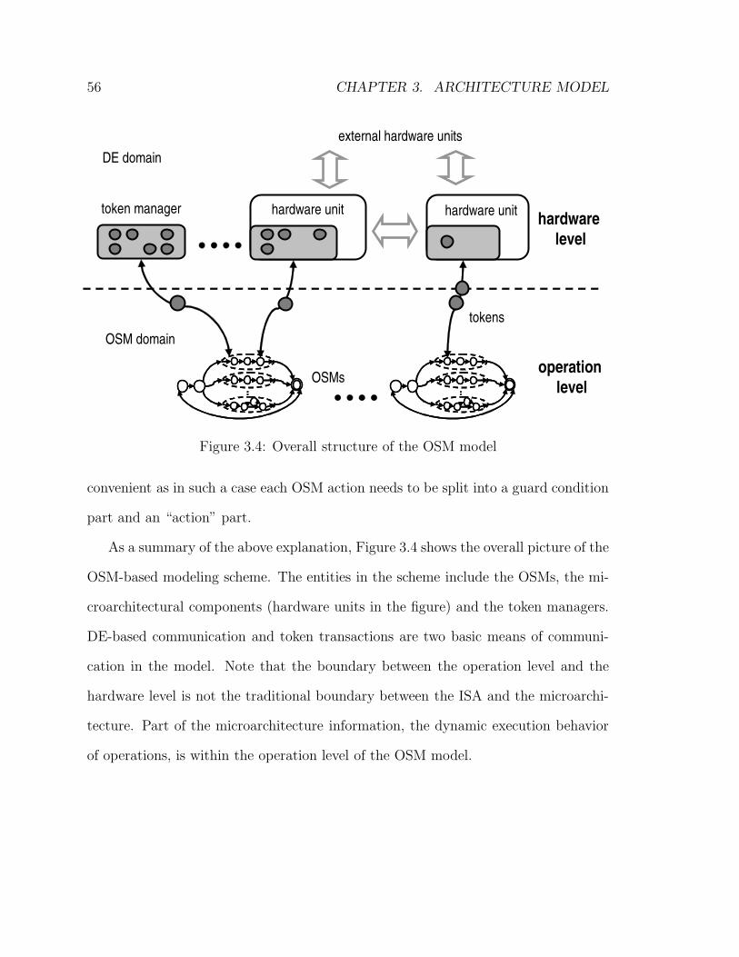
56 CHAPTER 3. ARCHITECTURE MODEL
hardware level
external hardware units
OSMsoperation
level
token manager hardware unit hardware unit
OSM domaintokens
DE domain
Figure 3.4: Overall structure of the OSM model
convenient as in such a case each OSM action needs to be split into a guard condition
part and an “action” part.
As a summary of the above explanation, Figure 3.4 shows the overall picture of the
OSM-based modeling scheme. The entities in the scheme include the OSMs, the mi-
croarchitectural components (hardware units in the figure) and the token managers.
DE-based communication and token transactions are two basic means of communi-
cation in the model. Note that the boundary between the operation level and the
hardware level is not the traditional boundary between the ISA and the microarchi-
tecture. Part of the microarchitecture information, the dynamic execution behavior
of operations, is within the operation level of the OSM model.
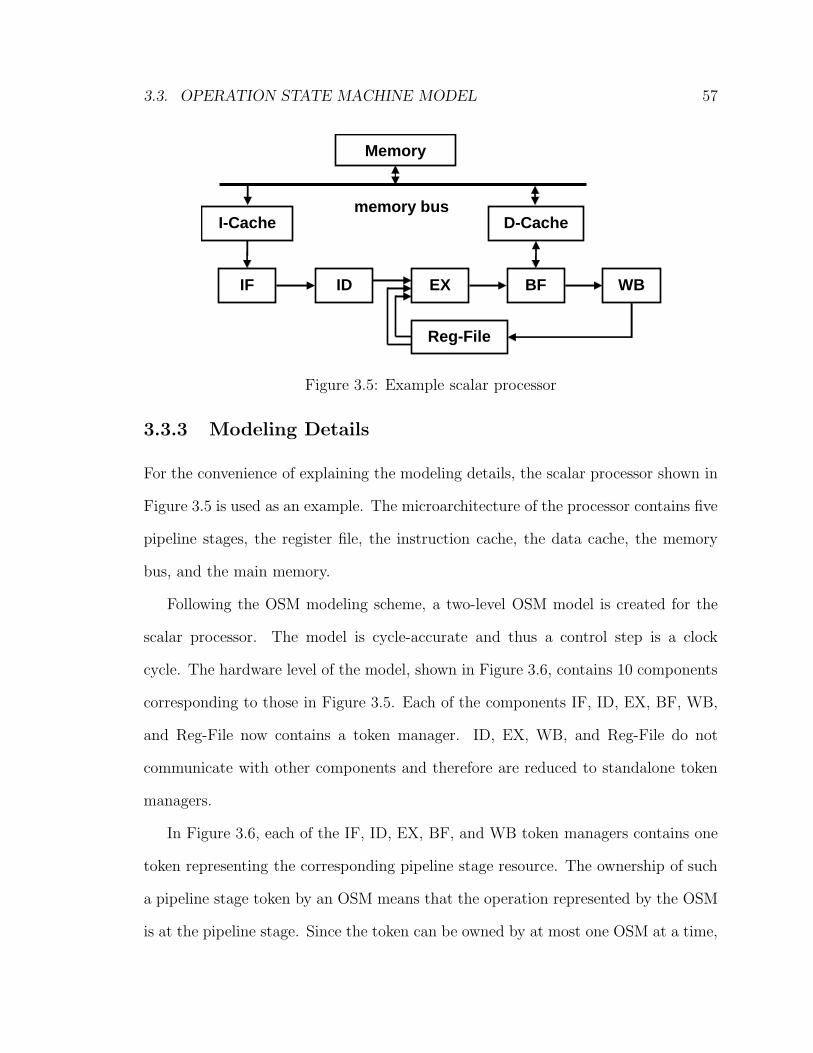
3.3. OPERATION STATE MACHINE MODEL 57
IF ID EX BF WB
I-Cache D-Cache
Memory
memory bus
Reg-File
Figure 3.5: Example scalar processor
3.3.3 Modeling Details
For the convenience of explaining the modeling details, the scalar processor shown in
Figure 3.5 is used as an example. The microarchitecture of the processor contains five
pipeline stages, the register file, the instruction cache, the data cache, the memory
bus, and the main memory.
Following the OSM modeling scheme, a two-level OSM model is created for the
scalar processor. The model is cycle-accurate and thus a control step is a clock
cycle. The hardware level of the model, shown in Figure 3.6, contains 10 components
corresponding to those in Figure 3.5. Each of the components IF, ID, EX, BF, WB,
and Reg-File now contains a token manager. ID, EX, WB, and Reg-File do not
communicate with other components and therefore are reduced to standalone token
managers.
In Figure 3.6, each of the IF, ID, EX, BF, and WB token managers contains one
token representing the corresponding pipeline stage resource. The ownership of such
a pipeline stage token by an OSM means that the operation represented by the OSM
is at the pipeline stage. Since the token can be owned by at most one OSM at a time,
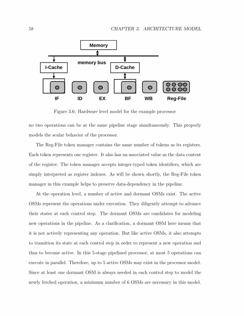
58 CHAPTER 3. ARCHITECTURE MODEL
I-Cache D-Cache
Memory
memory bus
WBBFEXIDIF Reg-File
Figure 3.6: Hardware level model for the example processor
no two operations can be at the same pipeline stage simultaneously. This properly
models the scalar behavior of the processor.
The Reg-File token manager contains the same number of tokens as its registers.
Each token represents one register. It also has an associated value as the data content
of the register. The token manager accepts integer-typed token identifiers, which are
simply interpreted as register indexes. As will be shown shortly, the Reg-File token
manager in this example helps to preserve data-dependency in the pipeline.
At the operation level, a number of active and dormant OSMs exist. The active
OSMs represent the operations under execution. They diligently attempt to advance
their states at each control step. The dormant OSMs are candidates for modeling
new operations in the pipeline. As a clarification, a dormant OSM here means that
it is not actively representing any operation. But like active OSMs, it also attempts
to transition its state at each control step in order to represent a new operation and
thus to become active. In this 5-stage pipelined processor, at most 5 operations can
execute in parallel. Therefore, up to 5 active OSMs may exist in the processor model.
Since at least one dormant OSM is always needed in each control step to model the
newly fetched operation, a minimum number of 6 OSMs are necessary in this model.
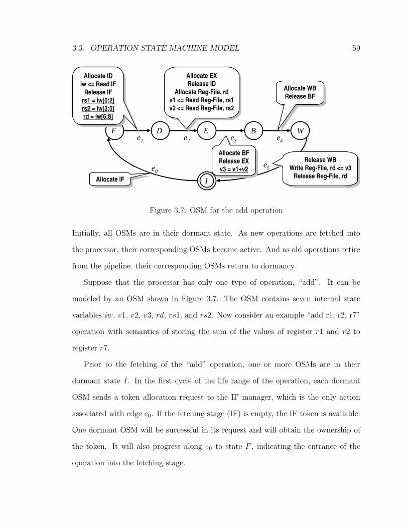
3.3. OPERATION STATE MACHINE MODEL 59
F D Ee1 e2
B W
I
e0
e3 e4
e5
Allocate IFAllocate IF
Allocate IDiw <= Read IF
Release IFrs1 = iw[0:2]rs2 = iw[3:5]rd = iw[6:8]
Allocate IDiw <= Read IF
Release IFrs1 = iw[0:2]rs2 = iw[3:5]rd = iw[6:8]
Allocate EXRelease ID
Allocate Reg-File, rdv1 <= Read Reg-File, rs1v2 <= Read Reg-File, rs2
Allocate EXRelease ID
Allocate Reg-File, rdv1 <= Read Reg-File, rs1v2 <= Read Reg-File, rs2
Allocate BFRelease EXv3 = v1+v2
Allocate BFRelease EXv3 = v1+v2
Allocate WBRelease BF
Allocate WBRelease BF
Release WBWrite Reg-File, rd <= v3
Release Reg-File, rd
Release WBWrite Reg-File, rd <= v3
Release Reg-File, rd
Figure 3.7: OSM for the add operation
Initially, all OSMs are in their dormant state. As new operations are fetched into
the processor, their corresponding OSMs become active. And as old operations retire
from the pipeline, their corresponding OSMs return to dormancy.
Suppose that the processor has only one type of operation, “add”. It can be
modeled by an OSM shown in Figure 3.7. The OSM contains seven internal state
variables iw, v1, v2, v3, rd, rs1, and rs2. Now consider an example “add r1, r2, r7”
operation with semantics of storing the sum of the values of register r1 and r2 to
register r7.
Prior to the fetching of the “add” operation, one or more OSMs are in their
dormant state I. In the first cycle of the life range of the operation, each dormant
OSM sends a token allocation request to the IF manager, which is the only action
associated with edge e0. If the fetching stage (IF) is empty, the IF token is available.
One dormant OSM will be successful in its request and will obtain the ownership of
the token. It will also progress along e0 to state F , indicating the entrance of the
operation into the fetching stage.
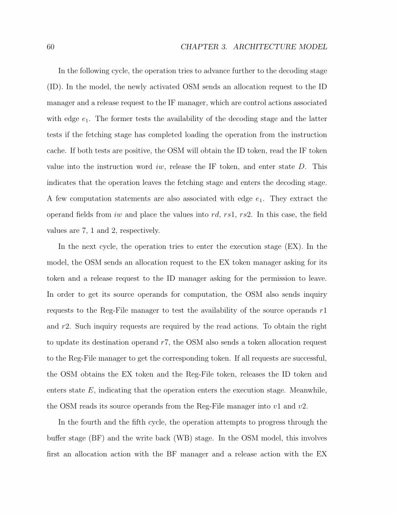
60 CHAPTER 3. ARCHITECTURE MODEL
In the following cycle, the operation tries to advance further to the decoding stage
(ID). In the model, the newly activated OSM sends an allocation request to the ID
manager and a release request to the IF manager, which are control actions associated
with edge e1. The former tests the availability of the decoding stage and the latter
tests if the fetching stage has completed loading the operation from the instruction
cache. If both tests are positive, the OSM will obtain the ID token, read the IF token
value into the instruction word iw, release the IF token, and enter state D. This
indicates that the operation leaves the fetching stage and enters the decoding stage.
A few computation statements are also associated with edge e1. They extract the
operand fields from iw and place the values into rd, rs1, rs2. In this case, the field
values are 7, 1 and 2, respectively.
In the next cycle, the operation tries to enter the execution stage (EX). In the
model, the OSM sends an allocation request to the EX token manager asking for its
token and a release request to the ID manager asking for the permission to leave.
In order to get its source operands for computation, the OSM also sends inquiry
requests to the Reg-File manager to test the availability of the source operands r1
and r2. Such inquiry requests are required by the read actions. To obtain the right
to update its destination operand r7, the OSM also sends a token allocation request
to the Reg-File manager to get the corresponding token. If all requests are successful,
the OSM obtains the EX token and the Reg-File token, releases the ID token and
enters state E, indicating that the operation enters the execution stage. Meanwhile,
the OSM reads its source operands from the Reg-File manager into v1 and v2.
In the fourth and the fifth cycle, the operation attempts to progress through the
buffer stage (BF) and the write back (WB) stage. In the OSM model, this involves
first an allocation action with the BF manager and a release action with the EX
3.3. OPERATION STATE MACHINE MODEL 61
manager, and subsequently an allocation action with the WB manager and a release
action with the BF manager. If all actions succeed, the OSM enters state W at
the fifth cycle and the operation gets into the WB stage. Note that a computation
expression exists on edge e3 of Figure 3.7. It evaluates the semantics of the operation.
In the last cycle of its life range, the operation aims to retire from the pipeline.
In the processor model, the OSM sends release requests to the WB manager and the
Reg-File manager. If both are successful, the OSM writes its computation result in v3
to the destination token and releases both tokens. It then goes back to the dormant
state I, finishing modeling the “add” operation. The OSM now owns no token. It is
ready to model another “add” operation in the following control step.
The above description explains the correlation between the model and the example
processor. The modeling details of some fundamental pipeline behaviors are described
as follows:
Pipelining At each control step, the active and the dormant OSMs diligently try to
advance their states. As a previous operation leaves a pipeline stage, its corre-
sponding OSM releases the token representing the pipeline stage. A following
OSM will then be able to obtain the token in the same control step and get into
the pipeline stage. This models the fully pipelined execution of the processor.
The release-by-one and allocate-to-another sequence in one control step is co-
ordinated by the scheduler. Details regarding scheduling are provided in Sec-
tion 3.3.5.
Structure Hazard In the example model, a pipeline stage token manager contains
only one token. Ownership of the token by an OSM means that the correspond-
ing operation is inside the pipeline stage represented by the token. Since the
62 CHAPTER 3. ARCHITECTURE MODEL
token can be owned by only one OSM at a time, at most one operation can
occupy the pipeline stage at a given time. This naturally resolves structural
hazards in the pipeline.
The idea can be generalized and applied to other types of resources such as
memory ports. It can also be extended to the case when more than one homo-
geneous resource exists. For instance, if the processor is capable of fetching two
operations simultaneously, the IF token manager can contain two tokens.
Variable Latency Variable operation latency occurs very often in processors. For
example, the latency of instruction cache access varies depending on whether
the access hits or misses. The computation latency in multipliers with an early
termination scheme also varies depending on the value of the operands [38].
To model such behavior, the release action is used to control the latency after
which an OSM can leave a pipeline stage. Suppose that an instruction cache
miss occurs when the OSM is in state F . The IF component is notified of
the cache miss through DE-based signaling, and hereby the token manager IF
gets the information as it shares states with the component. When the OSM
attempts to proceed to state D in the following cycles, the token manager IF
rejects its token release request until the cache access is finished. Since the
state transition condition is the conjunction of all responses to the requests on
an edge, the condition fails and the OSM has to stall in state F until the cache
access is done. The same scheme can be used to cover other types of variable
latency behavior.
Data Hazard The Reg-File token manager serves to resolve data hazards. In the
example model, the OSM owns the token corresponding to its destination reg-
3.3. OPERATION STATE MACHINE MODEL 63
ister r7 from state E to state W . During this period, suppose the following
operation “add r7, r4, r3” enters the pipeline. Since this operation uses r7 as
its source operand, its OSM will send an inquiry request to the Reg-File man-
ager asking for the availability of the operand. Knowing that the r7 token is
held by the first OSM, the Reg-File manager rejects the request and the OSM
has to stall at D until the earlier operation finishes its computation and releases
the r7 token. Data dependency is thus preserved in this way.
3.3.4 Modeling of Common Processor Features
The example processor used so far is a very simple one with only one type of operation.
It lacks many basic operations of a real world processor such as branching and memory
access operations. Neither is it an efficient implementation since it does not have data
forwarding capability. This section explains how to model common features of modern
processors.
Instruction Set The OSM in Figure 3.7 models only one kind of operation. To
model a full instruction set, a more sophisticated OSM as shown in Figure 3.8
is needed. The new OSM is comprehensive in that it is capable of representing
all types of operations in the ISA. In its state diagram, states I, F , and D
are still shared among all the operations. After D, the state diagram splits
into multiple paths. Each path models the execution behavior of one type of
operation.
To steer an OSM to the right execution path matching the operation that it
represents, an artificial token manager named Decode is created. As a pure

64 CHAPTER 3. ARCHITECTURE MODEL
IDF
BE W
add
subBE W
inst-n
B1E WB2
Inquire Decode, (iw, 1)Inquire Decode, (iw, 1)
Inquire Decode, (iw, 2)Inquire Decode, (iw, 2)
Inquire Decode, (iw, n)Inquire Decode, (iw, n)
Figure 3.8: Comprehensive OSM for an instruction set
abstraction of the steering mechanism, Decode contains no token. It responds
to inquiry requests with token identifiers in the form of (integer, integer). The
first integer contains the instruction word, and the second contains an index
denoting the type of an operation. If the instruction word decodes to the type
as specified by the index, the inquiry request is approved by the token manager.
Otherwise, it is rejected.
In Figure 3.8, an inquiry action to Decode exists on each output edge from state
D. The instruction word value in iw and an index value unique to the operation
type corresponding to the edge are used as the token identifier. In this way, the
OSM can only proceed along the edge that matches the actual operation type.
More on Data Hazard The simple data hazard handling scheme described in Sec-
tion 3.3.3 does not handle write-after-write (WAW) hazards efficiently. Suppose
that the successor of the “add r1, r2, r7” operation is an “add r2, r3, r7”. As
the original operation holds the r7 token from state E to W , the successor can-
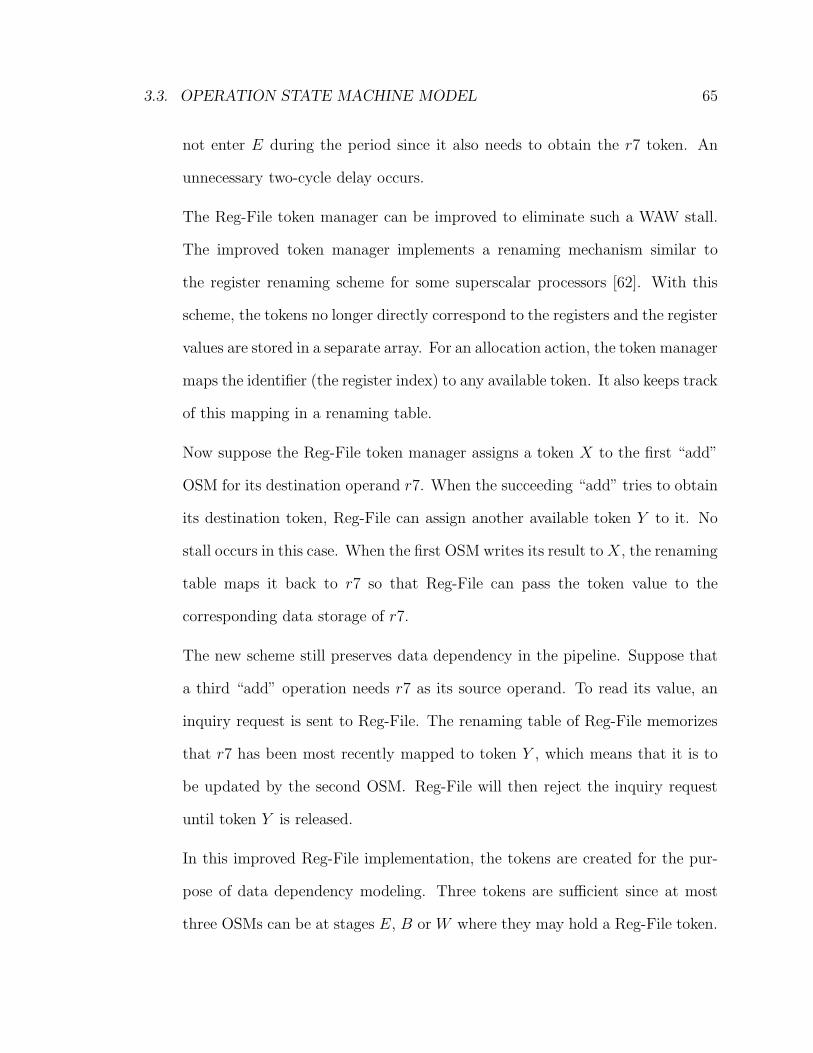
3.3. OPERATION STATE MACHINE MODEL 65
not enter E during the period since it also needs to obtain the r7 token. An
unnecessary two-cycle delay occurs.
The Reg-File token manager can be improved to eliminate such a WAW stall.
The improved token manager implements a renaming mechanism similar to
the register renaming scheme for some superscalar processors [62]. With this
scheme, the tokens no longer directly correspond to the registers and the register
values are stored in a separate array. For an allocation action, the token manager
maps the identifier (the register index) to any available token. It also keeps track
of this mapping in a renaming table.
Now suppose the Reg-File token manager assigns a token X to the first “add”
OSM for its destination operand r7. When the succeeding “add” tries to obtain
its destination token, Reg-File can assign another available token Y to it. No
stall occurs in this case. When the first OSM writes its result to X, the renaming
table maps it back to r7 so that Reg-File can pass the token value to the
corresponding data storage of r7.
The new scheme still preserves data dependency in the pipeline. Suppose that
a third “add” operation needs r7 as its source operand. To read its value, an
inquiry request is sent to Reg-File. The renaming table of Reg-File memorizes
that r7 has been most recently mapped to token Y , which means that it is to
be updated by the second OSM. Reg-File will then reject the inquiry request
until token Y is released.
In this improved Reg-File implementation, the tokens are created for the pur-
pose of data dependency modeling. Three tokens are sufficient since at most
three OSMs can be at stages E, B or W where they may hold a Reg-File token.
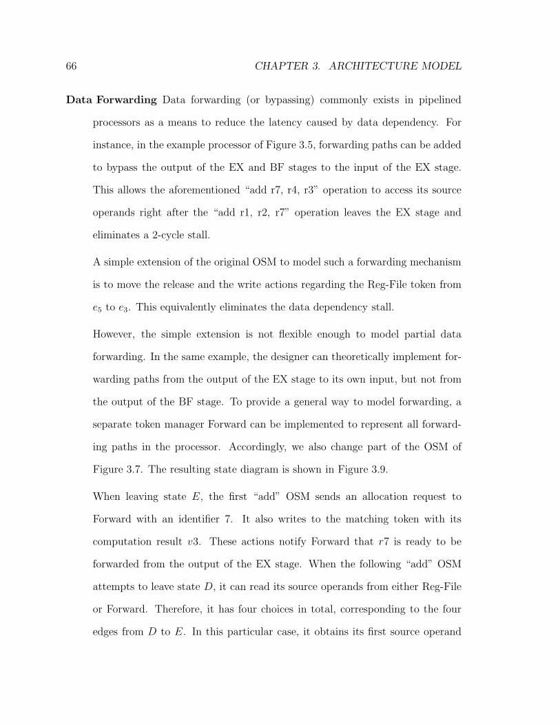
66 CHAPTER 3. ARCHITECTURE MODEL
Data Forwarding Data forwarding (or bypassing) commonly exists in pipelined
processors as a means to reduce the latency caused by data dependency. For
instance, in the example processor of Figure 3.5, forwarding paths can be added
to bypass the output of the EX and BF stages to the input of the EX stage.
This allows the aforementioned “add r7, r4, r3” operation to access its source
operands right after the “add r1, r2, r7” operation leaves the EX stage and
eliminates a 2-cycle stall.
A simple extension of the original OSM to model such a forwarding mechanism
is to move the release and the write actions regarding the Reg-File token from
e5 to e3. This equivalently eliminates the data dependency stall.
However, the simple extension is not flexible enough to model partial data
forwarding. In the same example, the designer can theoretically implement for-
warding paths from the output of the EX stage to its own input, but not from
the output of the BF stage. To provide a general way to model forwarding, a
separate token manager Forward can be implemented to represent all forward-
ing paths in the processor. Accordingly, we also change part of the OSM of
Figure 3.7. The resulting state diagram is shown in Figure 3.9.
When leaving state E, the first “add” OSM sends an allocation request to
Forward with an identifier 7. It also writes to the matching token with its
computation result v3. These actions notify Forward that r7 is ready to be
forwarded from the output of the EX stage. When the following “add” OSM
attempts to leave state D, it can read its source operands from either Reg-File
or Forward. Therefore, it has four choices in total, corresponding to the four
edges from D to E. In this particular case, it obtains its first source operand
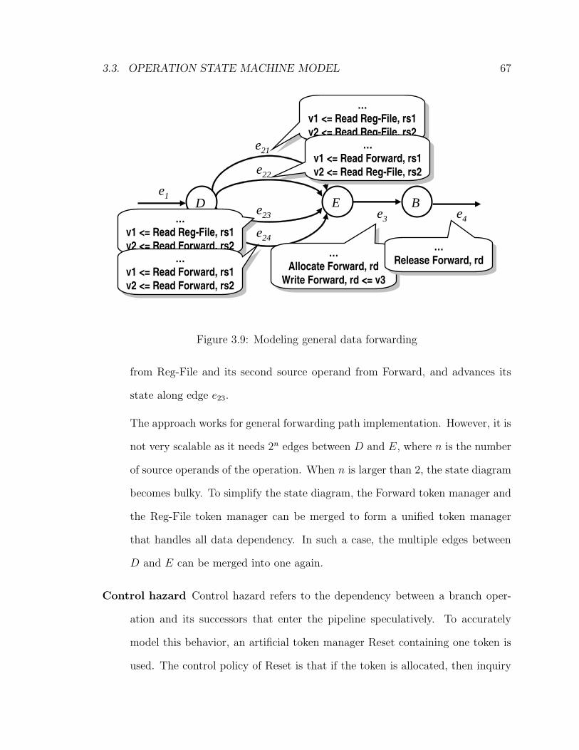
3.3. OPERATION STATE MACHINE MODEL 67
D E
e22
e3
…v1 <= Read Reg-File, rs1v2 <= Read Reg-File, rs2
…v1 <= Read Reg-File, rs1v2 <= Read Reg-File, rs2
e1
e21 …v1 <= Read Forward, rs1v2 <= Read Reg-File, rs2
…v1 <= Read Forward, rs1v2 <= Read Reg-File, rs2
e23
e24
…Allocate Forward, rd
Write Forward, rd <= v3
…Allocate Forward, rd
Write Forward, rd <= v3
Be4
…Release Forward, rd
…Release Forward, rd
…v1 <= Read Reg-File, rs1v2 <= Read Forward, rs2
…v1 <= Read Reg-File, rs1v2 <= Read Forward, rs2
…v1 <= Read Forward, rs1v2 <= Read Forward, rs2
…v1 <= Read Forward, rs1v2 <= Read Forward, rs2
Figure 3.9: Modeling general data forwarding
from Reg-File and its second source operand from Forward, and advances its
state along edge e23.
The approach works for general forwarding path implementation. However, it is
not very scalable as it needs 2n edges between D and E, where n is the number
of source operands of the operation. When n is larger than 2, the state diagram
becomes bulky. To simplify the state diagram, the Forward token manager and
the Reg-File token manager can be merged to form a unified token manager
that handles all data dependency. In such a case, the multiple edges between
D and E can be merged into one again.
Control hazard Control hazard refers to the dependency between a branch oper-
ation and its successors that enter the pipeline speculatively. To accurately
model this behavior, an artificial token manager Reset containing one token is
used. The control policy of Reset is that if the token is allocated, then inquiry

68 CHAPTER 3. ARCHITECTURE MODEL
F D Ee1 e2
Ie0
e3
ereset_1ereset_0Inquire ResetDiscard IF
Inquire ResetDiscard IF Inquire Reset
Discard IDInquire Reset
Discard ID
Figure 3.10: Augmented OSM with resetting capability
requests succeed. Otherwise, they fail. With this addition, the original OSM
in Figure 3.7 is also augmented with two edges from states F and D to state I.
Each edge contains one inquire action with Reset and one discard action, as is
shown in Figure 3.10. These edges are called reset-edges. In normal situations,
the inquiry requests will fail and these edges have no effect.
Now suppose that a branch mis-prediction occurs and two OSMs speculatively
enter state F and D, respectively. When the mis-predicted branch operation
leaves state E where the branch condition is resolved, it obtains the token from
Reset. In the same control step, the two speculative OSMs will evaluate the
condition on their reset-edges. In this case, since the Reset token is allocated,
the inquiry requests from the speculative OSMs succeed. As discard actions
are unconditional, the conditions on the reset-edges become true. Therefore,
the two OSMs change their states along the reset-edges. In other words, the
speculative operations are killed. In the next cycle, the branch OSM releases
the Reset token and the pipeline will function as normal.
An issue here is the priority of the multiple outgoing edges from the same state.
Suppose that both e2 and ereset 1 in Figure 3.10 are ready for state transition,
3.3. OPERATION STATE MACHINE MODEL 69
which one should the OSM prefer? As will be explained in Section 3.3.5, such
preference is statically determined. In this example, edge ereset 1 is preferred.
In summary, the OSM model can flexibly model the above common features. One
feature not mentioned is interrupt handling. To model this, an interrupt handler
should be implemented in the hardware level. It communicates with related compo-
nents such as the instruction fetcher IF. The effect of servicing an interrupt in the
operation level is similar to that of a branch operation.
3.3.5 Scheduling
The OSM model contains two levels. Therefore, its scheduling consists of three parts:
the hardware level, the operation level, and the coordination between the two levels.
The hardware level utilizes a standard DE scheduler. In contrast, the operation level
uses a specially designed OSM scheduler. The OSM scheduler addresses three issues
as described below.
1. Ordering of the fan-out edges
A state of an OSM may have multiple fan-out edges. A question arises when
multiple fan-out edges from the current state are ready for state transition.
Which one should the OSM choose? The rule for resolving this is that the
multiple edges are statically ordered. The ready edge with the highest priority
is used for state transition.
The static ordering scheme reflects common operation execution behavior. For
example, in Figure 3.2, the OSM always prefers e2 to e3, since when all resources
are available, the operation should execute, not wait. Similarly, in Figure 3.10,
the OSM would prefer the reset edges to e1 or e2. However, in theory there
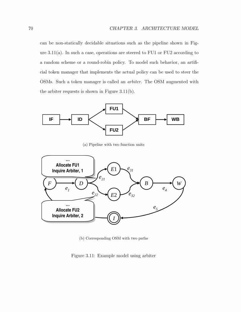
70 CHAPTER 3. ARCHITECTURE MODEL
can be non-statically decidable situations such as the pipeline shown in Fig-
ure 3.11(a). In such a case, operations are steered to FU1 or FU2 according to
a random scheme or a round-robin policy. To model such behavior, an artifi-
cial token manager that implements the actual policy can be used to steer the
OSMs. Such a token manager is called an arbiter. The OSM augmented with
the arbiter requests is shown in Figure 3.11(b).
IF ID
FU1
FU2
BF WB
(a) Pipeline with two function units
F D
E1
e1
e21B W
I
e0
e31
e4
e5
E2 e32e22
…Allocate FU1
Inquire Arbiter, 1
…Allocate FU1
Inquire Arbiter, 1
…Allocate FU2
Inquire Arbiter, 2
…Allocate FU2
Inquire Arbiter, 2
(b) Corresponding OSM with two paths
Figure 3.11: Example model using arbiter
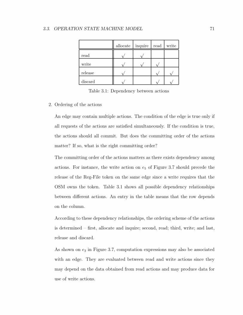
3.3. OPERATION STATE MACHINE MODEL 71
allocate inquire read write
read√ √
write√ √ √
release√ √ √
discard√ √ √
Table 3.1: Dependency between actions
2. Ordering of the actions
An edge may contain multiple actions. The condition of the edge is true only if
all requests of the actions are satisfied simultaneously. If the condition is true,
the actions should all commit. But does the committing order of the actions
matter? If so, what is the right committing order?
The committing order of the actions matters as there exists dependency among
actions. For instance, the write action on e5 of Figure 3.7 should precede the
release of the Reg-File token on the same edge since a write requires that the
OSM owns the token. Table 3.1 shows all possible dependency relationships
between different actions. An entry in the table means that the row depends
on the column.
According to these dependency relationships, the ordering scheme of the actions
is determined – first, allocate and inquire; second, read; third, write; and last,
release and discard.
As shown on e3 in Figure 3.7, computation expressions may also be associated
with an edge. They are evaluated between read and write actions since they
may depend on the data obtained from read actions and may produce data for
use of write actions.
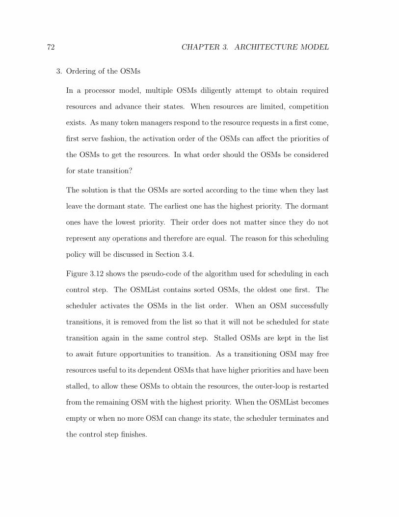
72 CHAPTER 3. ARCHITECTURE MODEL
3. Ordering of the OSMs
In a processor model, multiple OSMs diligently attempt to obtain required
resources and advance their states. When resources are limited, competition
exists. As many token managers respond to the resource requests in a first come,
first serve fashion, the activation order of the OSMs can affect the priorities of
the OSMs to get the resources. In what order should the OSMs be considered
for state transition?
The solution is that the OSMs are sorted according to the time when they last
leave the dormant state. The earliest one has the highest priority. The dormant
ones have the lowest priority. Their order does not matter since they do not
represent any operations and therefore are equal. The reason for this scheduling
policy will be discussed in Section 3.4.
Figure 3.12 shows the pseudo-code of the algorithm used for scheduling in each
control step. The OSMList contains sorted OSMs, the oldest one first. The
scheduler activates the OSMs in the list order. When an OSM successfully
transitions, it is removed from the list so that it will not be scheduled for state
transition again in the same control step. Stalled OSMs are kept in the list
to await future opportunities to transition. As a transitioning OSM may free
resources useful to its dependent OSMs that have higher priorities and have been
stalled, to allow these OSMs to obtain the resources, the outer-loop is restarted
from the remaining OSM with the highest priority. When the OSMList becomes
empty or when no more OSM can change its state, the scheduler terminates and
the control step finishes.
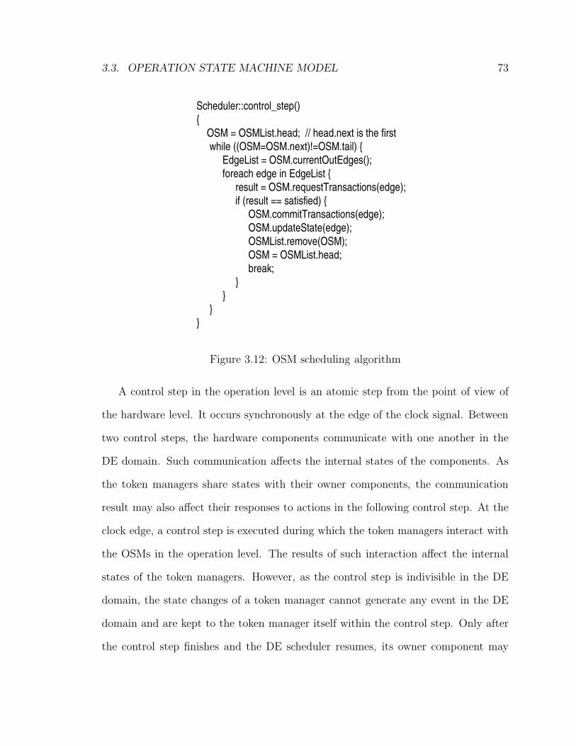
3.3. OPERATION STATE MACHINE MODEL 73
Scheduler::control_step() {
OSM = OSMList.head; // head.next is the firstwhile ((OSM=OSM.next)!=OSM.tail) {
EdgeList = OSM.currentOutEdges();foreach edge in EdgeList {
result = OSM.requestTransactions(edge);if (result == satisfied) {
OSM.commitTransactions(edge); OSM.updateState(edge);OSMList.remove(OSM);OSM = OSMList.head;break;
}}
}}
Figure 3.12: OSM scheduling algorithm
A control step in the operation level is an atomic step from the point of view of
the hardware level. It occurs synchronously at the edge of the clock signal. Between
two control steps, the hardware components communicate with one another in the
DE domain. Such communication affects the internal states of the components. As
the token managers share states with their owner components, the communication
result may also affect their responses to actions in the following control step. At the
clock edge, a control step is executed during which the token managers interact with
the OSMs in the operation level. The results of such interaction affect the internal
states of the token managers. However, as the control step is indivisible in the DE
domain, the state changes of a token manager cannot generate any event in the DE
domain and are kept to the token manager itself within the control step. Only after
the control step finishes and the DE scheduler resumes, its owner component may
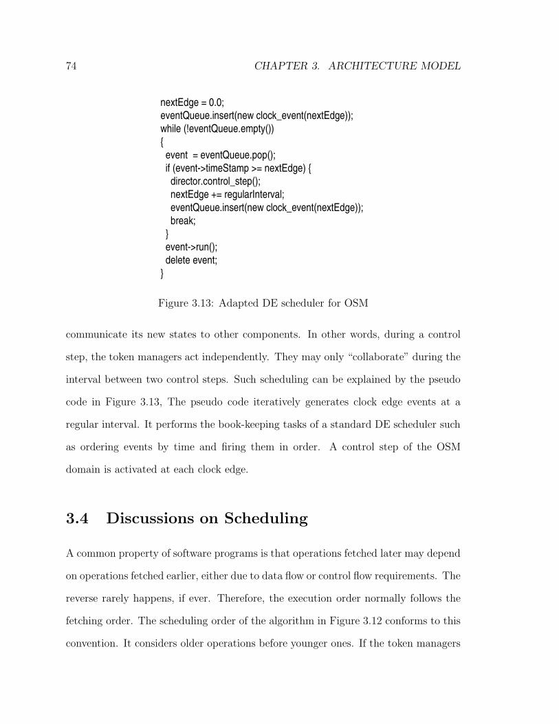
74 CHAPTER 3. ARCHITECTURE MODEL
nextEdge = 0.0;eventQueue.insert(new clock_event(nextEdge));while (!eventQueue.empty()){
event = eventQueue.pop();if (event->timeStamp >= nextEdge) {
director.control_step();nextEdge += regularInterval;eventQueue.insert(new clock_event(nextEdge));break;
}event->run();delete event;
}
Figure 3.13: Adapted DE scheduler for OSM
communicate its new states to other components. In other words, during a control
step, the token managers act independently. They may only “collaborate” during the
interval between two control steps. Such scheduling can be explained by the pseudo
code in Figure 3.13, The pseudo code iteratively generates clock edge events at a
regular interval. It performs the book-keeping tasks of a standard DE scheduler such
as ordering events by time and firing them in order. A control step of the OSM
domain is activated at each clock edge.
3.4 Discussions on Scheduling
A common property of software programs is that operations fetched later may depend
on operations fetched earlier, either due to data flow or control flow requirements. The
reverse rarely happens, if ever. Therefore, the execution order normally follows the
fetching order. The scheduling order of the algorithm in Figure 3.12 conforms to this
convention. It considers older operations before younger ones. If the token managers
3.4. DISCUSSIONS ON SCHEDULING 75
assign available resources in a first come, first serve style, the earlier fetched operations
always have the priority to obtain resources. Such a scheduler is straightforward to
implement and has predictable outcome.
However, in out-of-order issuing processors, the execution order does not necessar-
ily follow the fetching order. When the processor determines (maybe speculatively)
that there exists no data or control dependency between two operations, it may issue
the younger one first even though the older one is also ready to execute. To model
such priority inversion behavior, the token manager related to the issuing control can
be implemented in such a way that it “hand-picks” its preferred OSM for resource
assignment: it may deliberately reject an earlier request from an older OSM and ap-
prove another later request from a younger OSM. Such a token management policy is
different from the usual practice to assign tokens according to the order of requests. It
implements the priority inversion control policy of the processor. This type of token
managers are also called arbiters.
Arbiters should be used with caution. Deadlock situations may arise as a result
of using two or more arbiters. For instance, if two OSMs α and β are competing for
resources from both arbiters M1 and M2. Suppose M1 prefers α for token assignment,
while M2 prefers β. Then neither α nor β can get both tokens simultaneously and
advance its state. Thus a deadlock occurs. The deadlock situation is caused by
conflicting resource allocation policies. A model that may lead to such a situation is
considered erroneous. The scheduler may detect deadlocks by using a timeout counter
for each active OSM. It may choose to abort if a deadlock is detected.
Deadlock situation may also occur in the scheduling algorithm as a result of cyclic
resource dependency involving two or more OSMs. For example, consider an OSM
α whose next state transition depends on an allocation request to M3 and a release
76 CHAPTER 3. ARCHITECTURE MODEL
request to M4, and an OSM β whose next state transition depends on an allocation
request to M4 and a release request to M3. In other words, α depends on β to release
its M3 token and β depends on α to release its M4 token. If α is scheduled first, its
allocation request to M3 fails since β has not released the token yet. Therefore α
stalls in its current state and cannot release its M4 token. When β is scheduled later,
it cannot get the M4 token since α is still holding it. As a result, neither one can
change its state and a deadlock occurs. The deadlock cannot be resolved even if the
scheduler reorders α and β.
The second deadlock situation is caused by the fact that the scheduler in Fig-
ure 3.12 considers the OSMs sequentially and that each token manager makes its
decision independently. The scheduler may also abort in this case. This type of dead-
lock is admittedly a limitation of the scheduler. However, in processor designs, such
cyclic dependency between operations is rarely observed. Therefore, it does not imply
a serious limitation of the OSM-based modeling approach. If such behavior does ever
exist in a processor, a workaround technique can be used to avoid the problem, as
will be described in Section 3.5.
In principle, it is possible to conceive of a simultaneous scheduler to avoid this
type of deadlock. In such a scheduler, all OSMs send all their requests on all outgoing
edges from their current states at the same time. The token managers then consider
all requests and reach a global decision that allows the maximum number of OSMs
to progress. The simultaneous scheduler may be implemented in two schemes.
The first scheme involves a global solver that takes into account all requests from
the OSMs, as well as the policies and the states of all token managers. The solver then
computes the schedule for the current control step as an optimization problem. The
scheme requires that the implementation details of all token managers be transparent
3.4. DISCUSSIONS ON SCHEDULING 77
to and analyzable by the global solver. This requirement is beyond the scope of the
dissertation since all token managers are currently viewed as black boxes. Therefore
they can be implemented in any suitable programming language.
The second scheme is based on the Heterogeneous Synchronous/Reactive (HSR)
MoC [17]. In an HSR system, the components are viewed as black boxes. They react
to their inputs instantaneously and generate corresponding outputs. The outputs may
further activate other components. The chain reaction continues until all components
in the system stabilize. The MoC has been used in the Liberty Simulation Environ-
ment for operation flow control modeling. Based on the HSR, the token managers
need to be enhanced with the capability to communicate with one another in order
to collectively reach a global decision. In the dead-lock example above, M3 needs to
communicate with M4 to reach coordinated responses to α and β. Such relationship
between M3 and M4 is determined by the OSMs as both token managers are involved
in the condition on an edge of α or β. In other words, the communication relation-
ships between token managers are determined by the specification of the OSMs. A
change in an OSM may hence affect the implementation of the token managers. This
violates the modularity principle in software design and is a serious drawback of the
approach. Moreover, for an HSR system to behave well, each component must satisfy
the monotonicity requirement [17], viz., a component cannot reverse its mind after it
makes a decision. The monotonicity property is hard to enforce when the components
are implemented in a general-purpose programming language. As a matter of fact,
the checking of such a property is not even implemented in Ptolemy [88], which is
the de facto standard MoC experimenting infrastructure. Therefore, it is possible
to introduce hazardous situations that cause unpredictable behaviors in the token
managers in this scheme.
78 CHAPTER 3. ARCHITECTURE MODEL
Overall, the advantage of resolving the cyclic dependency deadlock by using an
HSR-based scheduler is not worthwhile due to its drawbacks. Therefore, this direction
is not explored any further.
3.5 Discussions of the OSM Model
The OSM model is a hybrid domain-specific MoC for processor modeling. The ad-
vantages of using the OSM model are summarized below.
First, compared to purely DE-based approaches, the OSM model features a higher
abstraction level. It allows designers to focus on high-level design decisions rather
than low level details. Due to the abstraction mechanisms of the operation level and
the token managers, the hardware structure of the model is greatly simplified. This
effect can be seen by comparing Figure 3.5 and Figure 3.6. The connectivity between
the microarchitecture components is largely simplified. Such reduction of structural
complexity makes the model compact. It also improves simulation efficiency as the
number of events is reduced in the DE-domain of the model.
Second, the OSM model supports the distribution of control semantics of a pro-
cessor among the token managers and the state diagrams of the OSMs. Such a
distributed control mechanism allows designers to conceive different control aspects
of the processor separately. This also helps to improve the modeling productivity.
Third, since the OSMs represent the behavior of operations, the modeling of the
operation level is straightforward as much information needed to specify the OSMs
can be found directly in the ISA manual. It is also easy to extract operation properties
from the state machines since the control and data semantics of the operations are
largely exposed by the state diagram and the actions on the edges. Therefore it is
3.5. DISCUSSIONS OF THE OSM MODEL 79
possible to infer processor properties from an OSM model for the use of compilers or
formal verification tools. In this sense, the OSM model is analyzable.
Finally, the OSM model combines the flexibility of finite state machines and the
DE MoC. It is therefore flexible enough to model a wide range of processors, including
scalar, superscalar, and VLIW ones.
The OSM model is not without its limitations. First, it abstracts only a sub-
set of all hardware components, viz., those directly interacting with operations. For
simple processors such as most embedded ones, this approach is very effective as a
major portion of the processor core can benefit from the abstraction. For instance,
in the five-stage pipelined processor of Figure 3.6, 7 out of the 10 components are
fully or partially modeled as token managers and therefore simplified. The situa-
tion is different for highly complex processors such as the Itanium II from Intel [54].
The processor contains function units such as multiple branch predictors, instruction
prefetching logics, 3-level memory subsystems with address translation, and bus con-
trol logic. These function units remain as DE components in the hardware level of
the OSM model. As these units may represent a major portion of the modeling effort,
the overall benefit of using the OSM abstractions is not as significant to model such
highly complex processors.
Second, for processors featuring centralized control such as the scoreboard [62], the
OSM approach may not be effective. In a straightforward model of such a processor,
an arbiter can be implemented to represent the centralized control. Each edge of the
OSMs contains one control action – an inquiry request to the aribter token manager
for its approval of state transition along the edge. Such a model would work in
general. However, there is little productivity advantage of using the OSM modeling
approach in this case since all pipeline control is modeled in the hardware layer. Also
80 CHAPTER 3. ARCHITECTURE MODEL
the resulting model is not analyzable in that pipeline control semantics are completely
hidden in the arbiter.
Considering the above limitations, the OSM model is most suitable for the model-
ing of embedded processors with low or moderate structural and control complexity.
It should be noted that in principle, the OSM model can be used to model ar-
bitrary processors. In the worst case, a model with a centralized arbiter such as
in the scoreboard case can always be used to represent all control paths of a pro-
cessor, although such a modeling approach may not be appealing. Similarly, the
cyclic-dependency deadlock in Section 3.4 can always be resolved by merging the to-
ken managers involved in the deadlock into one arbiter. The down side is that the
analyzability of the resulting model degrades as resource transactions involving the
related tokens become obscure. The best practice for OSM-based processor modeling
is to always make the pipeline control as explicit as possible by using separate token
managers for different control policies.
Often, for simulator generation purposes, it is desirable that the ISA specification
(the instruction semantics) be separate from the microarchitecture description. In
such a case, the same ISA specification can remain constant as the microarchitecture
changes. For CAS generation, an ISS simulator utilizing the ISA specification can
be tightly coupled with the microarchitecture simulator. The former simulates in-
struction semantics, while the latter models timing. Such simulation style has been
adopted in SimpleScalar [4] and LSE [92]. It is possible to utilize the OSM model
in the same style. The instruction semantics can be removed from the operation
level of the OSM model and specified separately. The operation level of the resulting
model contains only the control behavior of the operations, such as using structural
resources and resolving operand dependency. The model can then be used to gen-
3.6. COMPARISON WITH OTHER ARCHITECTURE MODELS 81
erate a partial simulator for timing information only. Interfacing techniques such as
the “capabilities” interface of LSE [48] can be used to couple the ISS and the timing
simulator.
3.6 Comparison with Other Architecture Models
The OSM model is sometimes misunderstood as a Petri-net variation as it utilizes the
similar notion of tokens as resources. A Petri-net is a graph-based model consisting
of places, transitions, and arcs [55]. The places hold tokens. An arc connects one
place with one transition. Depending on the direction of the arc, the place may be
an input place or an output place of the transition. An arc is labeled with an integer
called cardinality. A transition may fire if each of its input places has no less tokens
than the cardinality of the corresponding arc. When it fires, tokens are removed from
each of its input places. The number of removed tokens from a place is the same as
the cardinality of its corresponding arc. Tokens are also added to the output places
of a transition during its firing. The number of added tokens to a place equals to
the cardinality of the corresponding output arc. Extensions to the Petri-net model
include Colored Petri-nets and Timed Colored Petri-nets. They added data flow and
timing modeling capability to the original net.
The OSM model appears similar to the Petri-net model because it also uses the
notion of token and the token-based firing condition. However, the OSM model is a
fundamentally different model. The key difference is that an OSM is sequential while
a Petri-net is concurrent. An OSM represents the execution status of one operation
and the concurrent execution of multiple OSMs forms the operation view a processor.
In comparison, a Petri-net itself is concurrent and therefore can be used to model the
82 CHAPTER 3. ARCHITECTURE MODEL
processor hardware directly. In Petri-net-based processor models [16, 98, 9], tokens
are often used to represent the operations flow and data flow rather than execution
resources.
Compared to the Petri-net-based modeling approaches, the OSM model features
a higher level of abstraction due to the existence of the operation level. This al-
lows the designer to separate the modeling of operation semantics from those of the
hardware components, which greatly simplifies the hardware components and their
communications. As a result, the OSM model potentially brings about higher mod-
eling productivity and efficiency. The same advantage applies when comparing the
OSM model with other structural modeling approaches such as DE, clock-driven, and
HSR. Although the hardware level of the OSM model is in the DE domain in the
general case, it is possible to simplify it and use a synchronous MoC for better simu-
lation efficiency. A simplified implementation of the hardware level will be described
in Chapter 5.
The Gantt-Chart model used by LISA [64] models operation flow control in
pipelines. It also features the explicit notion of operation and therefore is of a similar
abstraction level as the OSM model. However, due to its limited expressiveness in
modeling the execution statuses of operations, it can model only in-order pipelines.
Therefore, it is less flexible than the OSM model. Moreover, the Gantt-Chart model
exposes only the allocation of pipeline stage resources in the model, while the OSM
model is capable of exposing other types of structural resources such as the memory
ports, as well as data and control dependencies. Therefore the OSM model is more
analyzable.
The architecture templates adopted by many ADLs are not as flexible as the
OSM model. For instance, the templates of TIE [94] only allow users to create
3.7. SUMMARY 83
new instructions and datapath components. In other words, the main architectural
features of its processors are fixed. Users can only extend the instruction set and
tune a few parameters such as memory sizes. Such limited flexibility is helpful for
Tensilica to ensure that its software tools, especially the HLL compiler, are applicable
to newly created template instances. Similar but less stringent constraints exist for
other architecture template models. In contrast, the OSM model does not assume
any predefined architectural feature of the processor. As pointed out in Section 3.5,
it can be used to model any type of processors in theory.
3.7 Summary
This chapter introduced the operation state machine (OSM) model for the purpose
of modeling processors. The model was originally presented in the Conference on
Design Automation and Test in Europe [69]. It contains two levels: the operation
level at which the dynamic execution behavior of the operations are represented;
and the hardware level at which the simplified microarchitecture is modeled. Two
abstraction mechanisms are used in the model. At the operation level, the execution
of an operation is modeled as an EFSM. In the hardware level, the resources are
modeled as tokens and resource control policies are modeled as token managers. The
EFSMs communicate with the token managers through a token transaction protocol,
which serves as the interface between the operation level and the hardware level.
In essence, the OSM model captures the concurrency within a processor at both
the operation level and the hardware level. It also captures the interaction between
the two levels. As the model explicitly represents the semantics of individual oper-
ations in the EFSMs, it is relatively easy to extract operation properties from the
84 CHAPTER 3. ARCHITECTURE MODEL
model. It also greatly simplifies the microarchitecture components as the operation
semantics and part of the pipeline control semantics are embedded in the EFSMs.
This results in improved modeling productivity and potentially improved execution
efficiency compared to structural modeling approaches.
The chapter showed the OSM-based modeling schemes for the most common be-
haviors in modern processors, such as pipelining, structural, control and data haz-
ards, variable latency, and data forwarding. It also described an efficient scheduling
algorithm for the operation level. Although scheduling deadlock may exist in the
algorithm, it is not a severe limitation as such a deadlock situation is very rare in
processors, if ever possible. A workaround technique to avoid scheduling deadlock is
also given.
Compared with other modeling approaches, the OSM model offers a unique com-
bination of compactness, flexibility, efficiency, and analyzability. It is suitable to be
used in the design flow of software programmable platforms.
Chapter 4
An Architecture Description
Language for Generation of
Software Tools
4.1 Introduction
The last chapter introduced the OSM model that addresses the issues of model devel-
opment productivity, modeling flexibility, simulation efficiency, and ease of extracting
model properties. It is suitable to be used as the semantic model of a specification
language for embedded processors at the architecture/microarchitecture level. This
chapter presents the design of such a specification language called the MESCAL Ar-
chitecture Description Language (MADL).
The main intended usage of MADL is to support the generation of software tools
that are involved in the design process of a software programmable platform. Such
software tools include the cycle-accurate simulator (CAS), the instruction set simula-
85
86 CHAPTER 4. AN ADL FOR GENERATION OF SOFTWARE TOOLS
tor (ISS), the high-level language (HLL) compiler, the assembler, and the disassem-
bler for the processor being developed. As the OSM model is executable and contains
cycle-accurate timing information, a complete specification of the model naturally
suffices to generate the CAS. The same specification should also suffice to generate
the ISS as it needs only a subset of the information required by the CAS, viz., the
operation semantics. The HLL compiler, the assembler, and the disassembler need
information from the operation level of the OSM model, as well as static operation
properties including assembly syntax and binary encodings. Therefore, these proper-
ties should also be included in MADL.
The current version MADL contains the operation level of the OSM model and the
static operation properties. The hardware level of the OSM model, including the token
managers and the structural hardware components, is not currently a part of MADL.
Instead, its implementation is provided in the general programming language C++.
The reason for this decision is three-fold. First, although the token managers have
well-defined communication interface with the OSMs, their internal implementation is
not yet formalized. Therefore, it is not very useful to create ad-hoc description syntax
to implement them as such a task can be equally achieved in C++. Second, because
the hardware units communicate with each other in the DE domain and there already
exist standard DE-based simulation frameworks such as SystemC [81], there is little
value to implement another one. Third, unlike the operation level information which
is shared by different tools, the hardware level information is only used for simulator
generation. Therefore, an imperative-style implementation in C++ is sufficient for
this purpose. However, the situation may change when high-level synthesis becomes
a target application of MADL. Such an application requires the formalization of the
token managers, which remains as a part of the future work. Incidentally, the C++
4.1. INTRODUCTION 87
implementation of the hardware level allows it to be directly monitored at simulation
time thanks to the availability of mature C++ debugging tools.
Among the various tools that MADL intends to support, the HLL compiler is
most complicated to develop. In general, an HLL compiler requires more informa-
tion than an executable processor specification. For instance, a processor invariably
contains several storage units such as the register files, the instruction counter, the
instruction word registers, etc. An executable processor specification may include
dynamic behaviors such as accesses to these storages by operations. However, it
does not necessarily understand the high-level semantics related to such accesses. On
the contrary, the HLL compiler does need to understand such semantics. It must
know high-level information such as the structures and the usages of the register files,
whether special-purpose registers such as address registers or accumulator registers
exist, whether delay slots are present, etc. Such information cannot be easily ex-
tracted from an executable processor specification even if it is based on the OSM
model. This is due to the fact that the definition of such high-level semantics is
dependent on the tools that utilize them. For example, the special notion of address
registers1 is irrelevant to an OSM-based CAS, but it may be important to an HLL
compiler. Therefore, such information is defined as tool-dependent. Compared to
the executable specification which has well-defined and unambiguous semantics, the
tool-dependent information relies on the interpretation of the tool. As the implemen-
tation of the tool changes over time, its required information may change accordingly.
For example, a basic HLL compiler may not need information regarding the mem-
ory structure of a processor. When performance-oriented memory optimizations are
involved, some coarse-grained memory information may become necessary. When
1These are the registers storing memory reference addresses in some DSP designs.
88 CHAPTER 4. AN ADL FOR GENERATION OF SOFTWARE TOOLS
power-oriented memory optimizations are further implemented, more memory pa-
rameters may be required. Overall, the tool-dependent information serves a narrow
tool scope and is more volatile. Therefore, it is helpful to separate it from the exe-
cutable specification. The latter can then remain stable and sharable by various tools
as the former evolves.
Because of such concerns, MADL is created with a two-layer description structure.
The first layer, named the core language, describes the operation level of the OSM
model as well as the static operation properties of assembly syntax and binary encod-
ings. This layer has well-defined semantics based on the OSM model and constitutes
the major part of a processor description. Section 4.2 of the chapter describes the
design of the core layer. The second layer describes tool-dependent information. As
descriptions in this layer are attached to the syntax elements in the core layer, they
are also called annotations. They supplement the core description by providing extra
processor information specific to the tool or special hints for the tool to analyze and
extract processor properties. Distinct from the core layer, the semantics of annota-
tions are subject to the interpretation of the software tools that use the information.
Although initially the layer was intended to be used by HLL compilers, it may also
be used by other tools. Section 4.3 describes the annotation layer.
The goal of the chapter is not to enumerate the syntax of MADL, but to present
the important design considerations and solutions involved in designing MADL. As
a result, only those syntax rules related to these presentation goals are described. A
reference manual with more syntax details is provided in Appendix A.
4.2. CORE LANGUAGE 89
4.2 Core Language
The core language is organized as a list of sections. It describes the operation level of
the OSM model and additional operation properties. This includes the specification
of the state diagrams of the OSMs, the actions and computations associated with the
edges, the assembly syntax, and the binary encoding of the operations. Although the
hardware level of the OSM model is not included in MADL, the names of the token
managers and their data-type properties need to be declared in the core language
so that the actions can refer to them. The data-type property of a token manager
includes the type of its token identifiers and the type of the optional data values
associated with its tokens. MADL supports the declaration of various common data-
types including signed and unsigned integer types of any width, floating point types,
the string type, and the void type. In addition, tuple types composed of a list of
the above basic types are also supported. These data-types can be used for token
manager declaration and for creating global constants and internal state variables of
the OSMs.
For the scalar processor example of Figure 3.5, its token managers can be specified
as shown in Figure 4.1. The “MANAGER” section contains the declaration of token
manager classes and instances. A token manager class corresponds to a C++ class
in actual implementation. In this example, the ID, EX, and WB token managers
all belong to the “simple manager” class and share the same implementation. A
“simple manager” takes no token index, and its token contains no data value. Thus
its data-type contains two voids. The IF and BF managers communicate with their
corresponding hardware components and are declared as different classes. The Reg-
File manager is also implemented as a different class. In this case it contains 8 16-bit
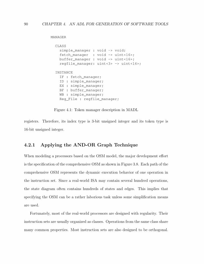
90 CHAPTER 4. AN ADL FOR GENERATION OF SOFTWARE TOOLS
MANAGER
CLASSsimple_manager : void -> void;fetch_manager : void -> uint<16>;buffer_manager : void -> uint<16>;regfile_manager: uint<3> -> uint<16>;
INSTANCEIF : fetch_manager;ID : simple_manager;EX : simple_manager;BF : buffer_manager;WB : simple_manager;Reg_File : regfile_manager;
Figure 4.1: Token manager description in MADL
registers. Therefore, its index type is 3-bit unsigned integer and its token type is
16-bit unsigned integer.
4.2.1 Applying the AND-OR Graph Technique
When modeling a processors based on the OSM model, the major development effort
is the specification of the comprehensive OSM as shown in Figure 3.8. Each path of the
comprehensive OSM represents the dynamic execution behavior of one operation in
the instruction set. Since a real-world ISA may contain several hundred operations,
the state diagram often contains hundreds of states and edges. This implies that
specifying the OSM can be a rather laborious task unless some simplification means
are used.
Fortunately, most of the real-world processors are designed with regularity. Their
instruction sets are usually organized as classes. Operations from the same class share
many common properties. Most instruction sets are also designed to be orthogonal.
4.2. CORE LANGUAGE 91
The operand fields are usually separate from one another and from the opcode field
in the binary encoding, allowing the addressing mode of each operand to be changed
independently. Such regular organization of the instruction set reduces the complex-
ity of the processor implementation. It also provides opportunities to simplify the
description of the OSMs in a similar hierarchical and orthogonal way. As mentioned
in Section 2.3.2, the AND-OR graph is a common syntax technique utilized by ex-
isting ADLs to exploit such regularity of the instruction set. MADL also uses this
technique to describe the OSMs.
In existing ADLs that utilize the AND-OR graph, such as LISA and nML, the
description of the operations is in reference to the pipeline stages. The static and
dynamic operation properties are broken into small description chunks, which are
then connected by some linkage description to form an AND-OR graph. The pipeline
stages form a graphical holding structure for the chunks of operation properties.
However, the situation is different in the OSM modeling approach. In an OSM, the
notion of the pipeline stages are replaced by tokens, which are circulating resources.
Thus they cannot serve as the holding structure for the operation chunks any more.
Instead, the holding structure of an OSM is its state diagram. The chunks, containing
the OSM actions, assembly syntax, and binary encodings, are bound to the edges of
the state diagram. As the comprehensive state diagram itself is quite large, specifying
the binding relationships remains tedious.
To solve the binding description problem, the OSM model is adapted to its dy-
namic version. The key idea is to replace the static binding relationship between the
state diagram and the operation chunks with a dynamic one. In the dynamic version,
the chunks are bound to the edges dynamically as the OSM executes. With this
scheme, a compact state diagram structure can be shared by all operations. In each
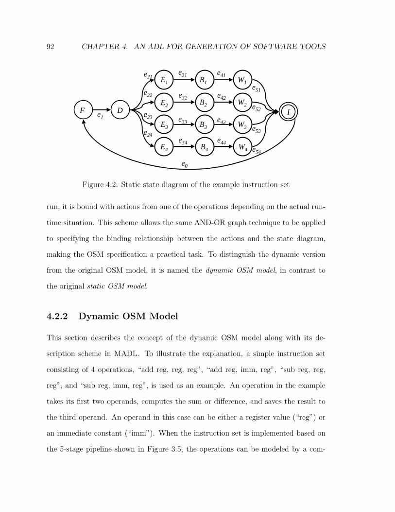
92 CHAPTER 4. AN ADL FOR GENERATION OF SOFTWARE TOOLS
F D
E4
e1
W4
I
e0
e34
E3 W3e33
E2 W2
e32
E1 W1
e31
B4
B3
B2
B1
e44
e43
e42
e41
e24
e23
e22
e21
e54
e53
e52
e51
Figure 4.2: Static state diagram of the example instruction set
run, it is bound with actions from one of the operations depending on the actual run-
time situation. This scheme allows the same AND-OR graph technique to be applied
to specifying the binding relationship between the actions and the state diagram,
making the OSM specification a practical task. To distinguish the dynamic version
from the original OSM model, it is named the dynamic OSM model, in contrast to
the original static OSM model.
4.2.2 Dynamic OSM Model
This section describes the concept of the dynamic OSM model along with its de-
scription scheme in MADL. To illustrate the explanation, a simple instruction set
consisting of 4 operations, “add reg, reg, reg”, “add reg, imm, reg”, “sub reg, reg,
reg”, and “sub reg, imm, reg”, is used as an example. An operation in the example
takes its first two operands, computes the sum or difference, and saves the result to
the third operand. An operand in this case can be either a register value (“reg”) or
an immediate constant (“imm”). When the instruction set is implemented based on
the 5-stage pipeline shown in Figure 3.5, the operations can be modeled by a com-
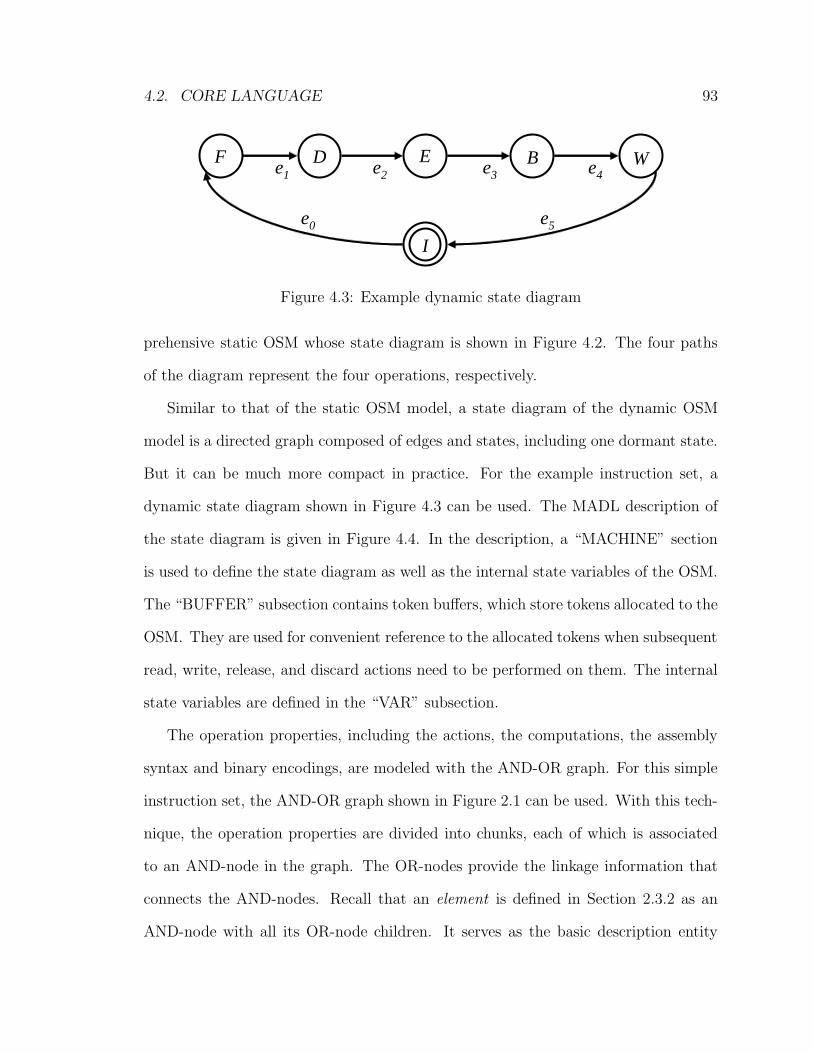
4.2. CORE LANGUAGE 93
F D Ee1 e2
B W
I
e0
e3 e4
e5
Figure 4.3: Example dynamic state diagram
prehensive static OSM whose state diagram is shown in Figure 4.2. The four paths
of the diagram represent the four operations, respectively.
Similar to that of the static OSM model, a state diagram of the dynamic OSM
model is a directed graph composed of edges and states, including one dormant state.
But it can be much more compact in practice. For the example instruction set, a
dynamic state diagram shown in Figure 4.3 can be used. The MADL description of
the state diagram is given in Figure 4.4. In the description, a “MACHINE” section
is used to define the state diagram as well as the internal state variables of the OSM.
The “BUFFER” subsection contains token buffers, which store tokens allocated to the
OSM. They are used for convenient reference to the allocated tokens when subsequent
read, write, release, and discard actions need to be performed on them. The internal
state variables are defined in the “VAR” subsection.
The operation properties, including the actions, the computations, the assembly
syntax and binary encodings, are modeled with the AND-OR graph. For this simple
instruction set, the AND-OR graph shown in Figure 2.1 can be used. With this tech-
nique, the operation properties are divided into chunks, each of which is associated
to an AND-node in the graph. The OR-nodes provide the linkage information that
connects the AND-nodes. Recall that an element is defined in Section 2.3.2 as an
AND-node with all its OR-node children. It serves as the basic description entity
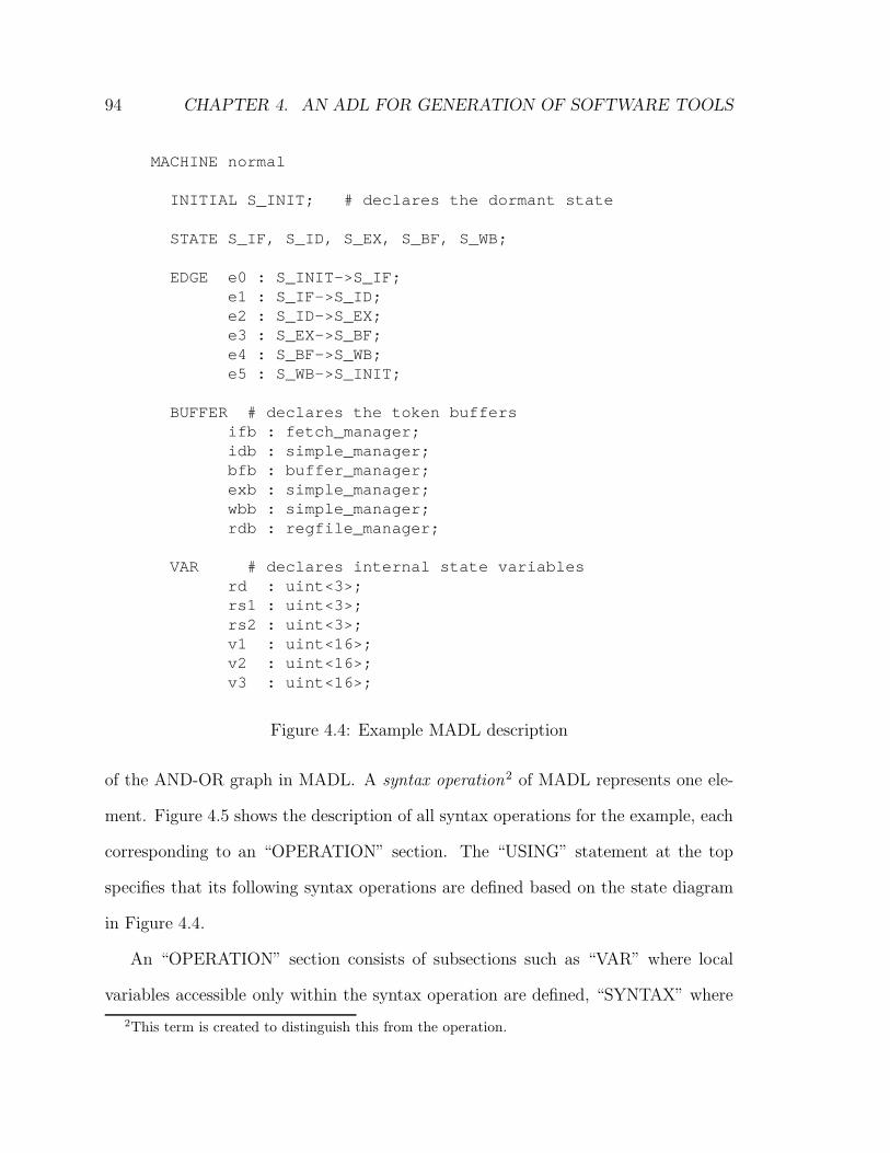
94 CHAPTER 4. AN ADL FOR GENERATION OF SOFTWARE TOOLS
MACHINE normal
INITIAL S_INIT; # declares the dormant state
STATE S_IF, S_ID, S_EX, S_BF, S_WB;
EDGE e0 : S_INIT->S_IF;e1 : S_IF->S_ID;e2 : S_ID->S_EX;e3 : S_EX->S_BF;e4 : S_BF->S_WB;e5 : S_WB->S_INIT;
BUFFER # declares the token buffersifb : fetch_manager;idb : simple_manager;bfb : buffer_manager;exb : simple_manager;wbb : simple_manager;rdb : regfile_manager;
VAR # declares internal state variablesrd : uint<3>;rs1 : uint<3>;rs2 : uint<3>;v1 : uint<16>;v2 : uint<16>;v3 : uint<16>;
Figure 4.4: Example MADL description
of the AND-OR graph in MADL. A syntax operation2 of MADL represents one ele-
ment. Figure 4.5 shows the description of all syntax operations for the example, each
corresponding to an “OPERATION” section. The “USING” statement at the top
specifies that its following syntax operations are defined based on the state diagram
in Figure 4.4.
An “OPERATION” section consists of subsections such as “VAR” where local
variables accessible only within the syntax operation are defined, “SYNTAX” where
2This term is created to distinguish this from the operation.
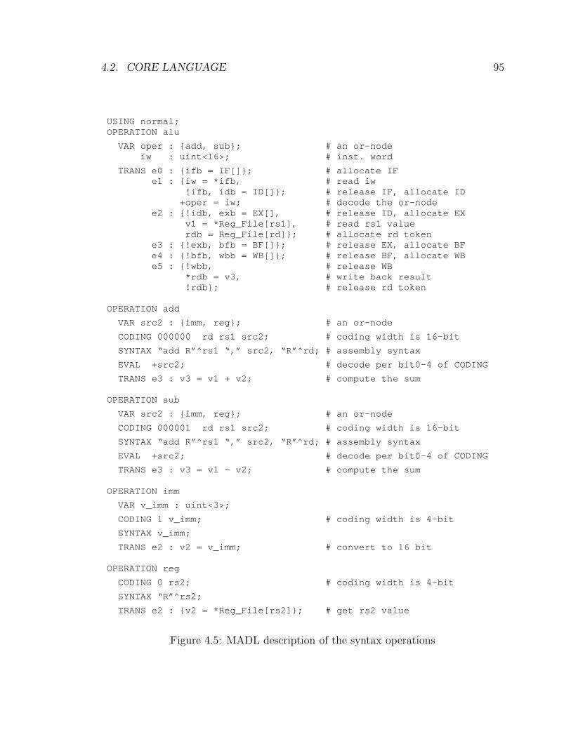
4.2. CORE LANGUAGE 95
USI NG nor mal ;OPERATI ON al u
VAR oper : { add, sub} ; # an or - nodei w : ui nt <16>; # i nst . wor d
TRANS e0 : { i f b = I F[ ] } ; # al l ocat e I Fe1 : { i w = * i f b, # r ead i w
! i f b, i db = I D[ ] } ; # r el ease I F, al l ocat e I D+oper = i w; # decode t he or - node
e2 : { ! i db, exb = EX[ ] , # r el ease I D, al l ocat e EXv1 = * Reg_Fi l e[ r s1] , # r ead r s1 val uer db = Reg_Fi l e[ r d] } ; # al l ocat e r d t oken
e3 : { ! exb, bf b = BF[ ] } ; # r el ease EX, al l ocat e BF e4 : { ! bf b, wbb = WB[ ] } ; # r el ease BF, al l ocat e WB e5 : { ! wbb, # r el ease WB
* r db = v3, # wr i t e back r esul t ! r db} ; # r el ease r d t oken
OPERATI ON add
VAR sr c2 : { i mm, r eg} ; # an or - node
CODI NG 000000 r d r s1 sr c2; # codi ng wi dt h i s 16- bi t
SYNTAX “ add R” ^ r s1 “ , ” sr c2, “ R” ^ r d; # assembl y synt ax
EVAL +sr c2; # decode per bi t 0- 4 of CODI NG
TRANS e3 : v3 = v1 + v2; # comput e t he sum
OPERATI ON sub
VAR sr c2 : { i mm, r eg} ; # an or - node
CODI NG 000001 r d r s1 sr c2; # codi ng wi dt h i s 16- bi t
SYNTAX “ add R” ^ r s1 “ , ” sr c2, “ R” ^ r d; # assembl y synt ax
EVAL +sr c2; # decode per bi t 0- 4 of CODI NG
TRANS e3 : v3 = v1 - v2; # comput e t he sum
OPERATI ON i mm
VAR v_i mm : ui nt <3>;
CODI NG 1 v_i mm; # codi ng wi dt h i s 4- bi t
SYNTAX v_i mm;
TRANS e2 : v2 = v_i mm; # conver t t o 16 bi t
OPERATI ON r eg
CODI NG 0 r s2; # codi ng wi dt h i s 4- bi t
SYNTAX “ R” ^ r s2;
TRANS e2 : { v2 = * Reg_Fi l e[ r s2] } ; # get r s2 val ue
Figure 4.5: MADL description of the syntax operations

96 CHAPTER 4. AN ADL FOR GENERATION OF SOFTWARE TOOLS
a chunk of assembly syntax is provided, “CODING” where a chunk of binary encod-
ing is specified, “EVAL” where variables can be initialized, and “TRANS” where a
chunk of actions and computations are defined with respect to the edges in the state
diagram. Actions are enclosed within curly braces, while computations are not. In a
“VAR” subsection, besides variables of normal arithmetic data types, a special type
of variable corresponding to the OR-nodes in the AND-OR graph can also be defined.
An example of such a variable is the “oper” variable in “alu” which corresponds to
the top OR-node in Figure 2.1. A special type of computation expression, decoding
expression, is used to decode such a variable during execution. The decoding expres-
sion will match the encoding of the children of the OR-node against a given integer
value (see “oper” in “alu”) or a part of the encoding of the its owner syntax operation
(see “src2” in “add”). The matching result resolves the identity of the OR-node as
one of its children.
During run time, the top-level syntax operation “alu” will be associated with
the state diagram first. Its actions and computations in the “TRANS” subsection
are bound to the corresponding edges. In this example, these include reading the
instruction word from the token manager IF and then decoding the OR-node variable
“oper” with the instruction word on edge e1. Depending on the value of the instruction
word, decoding will resolve “oper” to either “add” or “sub”. If the result is “add”,
then it will also bind the “TRANS” information of “add” to the edges of the same
state diagram. Meanwhile as the encoding of the “add” is known, the decoding
process propagates down to its OR-node variable “src2”. Based on the lowest five
bits of the encoding value of “add”, the variable will be resolved to either “imm” or
“reg”. If the result is “imm”, it will in turn bind its “TRANS” information to the
state diagram. The combined information from “alu”, “add”, “imm”, and the state
4.2. CORE LANGUAGE 97
diagram forms the model for an add-immediate instruction. Together, these syntax
operations correspond to one expansion in the AND-OR graph. In the case when
the instruction word decodes to a different expansion, the same state diagram can be
used, but bound with different actions and computations. The decoding mechanism
ensures that at run time, only one expansion is bound to the state diagram. With
such dynamic binding mechanism, the Decode manager used to steer the execution of
the comprehensive OSM in Section 3.3.4 is no longer needed in the dynamic model.
4.2.3 Converting the Dynamic OSM model
As with the static OSM model, the dynamic OSM model is also executable, although
its execution may be less efficient due to the overhead incurred by dynamic binding.
In the dynamic OSM model, an edge ex is said to dominate another edge ey if
every path from the dormant state to ey goes through ex. A decoding edge is defined
as the location where an OR-node variable is decoded with a given value. Such an
OR-node is called decoding node. In the above example, edge e1 is a decoding edge
as the value iw is used to decode the decoding node “oper” on the edge. A dynamic
OSM is said to be well-defined if each decoding edge dominates all the edges that
are involved in the dynamic binding as a result of the decoding. The example of
Figure 4.5 is a well-defined dynamic OSM as e1 dominates all the edges appearing
in the “TRANS” subsections of “add”, “sub”, “imm”, and “reg”. However, if the
“TRANS” subsection of “add” contains an action on edge e0, then the OSM is not
well defined since e1 does not dominate e0. The well-definedness property is necessary
to ensure the causality between binding and execution.
98 CHAPTER 4. AN ADL FOR GENERATION OF SOFTWARE TOOLS
A simple transformation can be performed to convert a well-defined dynamic
model to a static OSM model. In the case when only one decoding node exists
in the dynamic OSM, the transformation steps are:
1. Construct an AND-OR graph according to the definition of the syntax opera-
tions and OR-node variables. Also bind the actions and computations of the
top-level AND-node to the state diagram.
2. For each expansion in the AND-OR graph, duplicate the portion of the state
diagram that is reachable from the decoding edge (not including itself) but
without going through the dormant state.
3. For each expansion, bind its corresponding duplicated sub-state-diagram with
its actions and computations.
4. Synthesize a token manager that can steer the execution of the static OSM to
the duplicated paths at the decoding point. The token manager serves the same
purpose as the one in Figure 3.8.
In the example of Figure 4.5, the decoding edge is e1. The portion of the state
diagram including e2, e3, and e4 are duplicated for the four expansions. The resulting
static state diagram is the same as the one in Figure 4.2. In this example, the edges
e4i all contain the same actions. The same holds for the edges e5i. Therefore, the
OSM can be optimized by merging the equivalent edges and states. The result is a
simplified state diagram shown in Figure 4.6.
The above optimization is called equivalent state merging. In general, two edges
are defined to be equivalent if they share the same set of actions and computations,
and have the same destination state. Two states are defined as equivalent if their

4.2. CORE LANGUAGE 99
F D
E4
e1I
e0
e34
E3
W3e33
E2
e32
E1
Be4
e24
e23
e22
e21
e5
e31
Figure 4.6: Merged static state diagram
outgoing edges are pair-wise equivalent. Two equivalent states can be merged by
deleting one state as well as its outgoing edges and re-directing all its incoming edges
to the other state. The merging process starts from the predecessor states of the
dormant state and iteratively works backward to check for existence of equivalent
states.
When more than one decoding node exists in the dynamic OSM, the transforma-
tion process can be performed hierarchically following the structure of the AND-OR
graph. The top-level decoding node in the AND-OR graph is transformed first. Then
the process descends down the AND-OR graph and low-level nodes are transformed
one after another.
Similar to the dynamic OSM model, the Statecharts model [29] also involves the
notions of state diagram and AND-OR graph. However, its treatment of these two
elements is different. In the dynamic OSM model, the AND-OR graph is used to
express the actions and computations, which are essentially properties associated to
the edges in the state diagram. When converting a dynamic OSM model to its static
version, each expansion of the AND-OR graph corresponds to an execution path of
100 CHAPTER 4. AN ADL FOR GENERATION OF SOFTWARE TOOLS
Figure 3.8. In contrast, in Statecharts, the AND-OR graph is used to represent the
states. Each expansion of its AND-OR graph corresponds to a state in the flattened
state transition diagram.
4.2.4 Additional Actions
To ease the specification of the OSM model, two more actions are introduced in
MADL: the temporary allocate and the comparison. A temporary allocate is the
combination of an allocate action followed by a discard action in the next cycle (if
the allocate request is successful and committed). A comparison action is simply
a comparison expression between two data values. Normal arithmetic comparison
operators can all be used. If the result of the expression evaluates to be true, then
the action succeeds. A comparison action can be converted to an inquire action with
an artificial token manager. A tuple consisting of its two operands serves as the token
index for the manager, which performs the comparison and responds to the request
according to the comparison result.
As these two actions can be converted to the original control actions, they can be
viewed as syntax sugar of MADL. Their introduction does not alter the semantics of
the original OSM model.
4.3 Annotations
The annotations are embedded in the core description for supplying tool-dependent
information to the software tools. They appear in the form of paragraphs. A para-
graph can be in either a single-line format or a block format. The former is preceded
by a “$” and runs through the end of the line while the latter is enclosed within a
4.3. ANNOTATIONS 101
pair of “$$”s. Multiple paragraphs can be attached to a syntax element in the core
description. A syntax element can be a variable declaration, a state/edge declaration,
an action or a computation expression, etc. After the MADL description is parsed,
users can access an annotation paragraph via the pointer to the syntax element object
that it is associated with. A set of interface functions are defined for such access.
Annotations for different tools may coexist in the same MADL description. To
avoid confusion in accessing them, namespace labels can be associated with annota-
tion paragraphs. A label corresponds to the tool-scope of its paragraph. Users can
easily filter irrelevant annotations according to the labels. By default, paragraphs
without a label belong to the global namespace and can be shared by all tools.
As many tools may benefit from the annotations, a generic annotation syntax is
created so that it can be easily adapted for specific needs. Figure 4.7 shows the syntax
in Backus-Naur Form.
The annotation syntax contains two types of statements: commands and rela-
tionships. The commands are used to supply hints or additional information to user
tools. Figure 4.8 shows a part of the “MANAGER” section of Figure 4.1 annotated
with two commands. The two annotation paragraphs are attached to the declara-
tion of the manager class “simple manager”. The first paragraph informs the tool
in the “COMP” namespace (in this case the HLL compiler) that this manager class
contains one resource unit. The HLL compiler can utilize such information to an-
alyze the resource usages of the operations in order to schedule them. The second
paragraph notifies the “CSIM” tool (in this case the CAS) that this manager uses
the template class “untyped manager” with a template argument of “1” as its C++
implementation in the simulator.
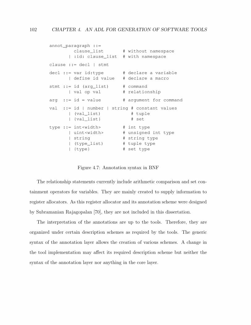
102 CHAPTER 4. AN ADL FOR GENERATION OF SOFTWARE TOOLS
annot_paragraph ::= clause_list # without namespace
| :id: clause_list # with namespace
clause ::= decl | stmt
decl ::= var id:type # declare a variable| define id value # declare a macro
stmt ::= id (arg_list) # command| val op val # relationship
arg ::= id = value # argument for command
val ::= id | number | string # constant values| (val_list) # tuple| {val_list} # set
type ::= int<width> # int type| uint<width> # unsigned int type| string # string type| (type_list) # tuple type| {type} # set type
Figure 4.7: Annotation syntax in BNF
The relationship statements currently include arithmetic comparison and set con-
tainment operators for variables. They are mainly created to supply information to
register allocators. As this register allocator and its annotation scheme were designed
by Subramanian Rajagopalan [70], they are not included in this dissertation.
The interpretation of the annotations are up to the tools. Therefore, they are
organized under certain description schemes as required by the tools. The generic
syntax of the annotation layer allows the creation of various schemes. A change in
the tool implementation may affect its required description scheme but neither the
syntax of the annotation layer nor anything in the core layer.

4.4. SUMMARY 103
MANAGER
CLASS
si mpl e_manager : voi d - > voi d;
$$ : COMP: SCHED_RESOURCE_TYPE( capaci t y=1) ; $$
$$ : CSI M: USE_CLASS( name=“ unt yped_manager ” ,
par am=“ 1” ) ; $$
……
Figure 4.8: Annotation description example
4.4 Summary
This chapter described the design of the MESCAL Architecture Description Language
(MADL), which mainly specifies OSMs. It is intended to be used by software tools
such as the CAS, the ISS, the assembler, the disassembler, and the HLL compiler.
As is generally required by the software tools, architecture descriptions contain
both well-defined model properties as well as ad-hoc tool-dependent information.
MADL adopts a two layer description scheme to separate the description of these two
types of information. The core layer of MADL specifies the executable OSM-based
processor model; while the annotation layer supplies extra information to the tools.
The layered approach insulates the core layer from frequent changes of the software
tools and therefore lengthens the life time of MADL descriptions.
The major design consideration of the core layer is to minimize the description
effort of the OSM model by using the AND-OR graph technique. Since binding
operation properties to the state diagram of a static OSM can be laborious due to
the potential huge size of the state diagram, a dynamic version of the OSM model was
introduced. In the dynamic OSM model, the operation properties are bound to its
compact state diagram at run-time. This technique integrates well with the AND-OR
104 CHAPTER 4. AN ADL FOR GENERATION OF SOFTWARE TOOLS
graph and thus forms the foundation of the core layer. A well-defined dynamic OSM
model can be converted back to the original OSM model by a simple transformation.
The annotation layer was designed with a generic syntax to flexibly support the
creation of description schemes. The use of the annotation layer by some software
tools will be described in the next chapter.
Chapter 5
Synthesis of Software Development
Tools
5.1 Introduction
Recall that in Figure 3.1, the critical software tools in the design flow of a software
programmable platform include a retargetable simulator and a retargetable high-
level language (HLL) compiler. The main goal of the operation state machine (OSM)
model and the MESCAL Architecture Description Language (MADL) described in
the previous two chapters is to support the generation of these software tools. This
chapter aims to demonstrate the effectiveness of the OSM model and MADL in this
regard.
As the OSM model is fully executable, it is straightforward to generate simulators
based on it. Mature techniques have been developed to synthesize very fast cycle-
accurate simulators (CAS) from MADL descriptions. Section 5.2 describes the CAS
105
106 CHAPTER 5. SYNTHESIS OF SOFTWARE DEVELOPMENT TOOLS
synthesis framework utilizing such techniques. The framework can also be modified for
instruction set simulator (ISS) generation. Section 5.3 describes such modifications. A
by-product of the simulator synthesis framework is an automated tool which generates
disassemblers from MADL descriptions. This tool is explained in Section 5.4.
Compared with simulators, an HLL compiler proves to be much more challenging
to develop. The key difficulty is providing for retargetability, or the capability to
automatically adapt the compiler for different instruction sets. For the wide variety
of possible existing instruction sets, different compilation flows and algorithms are
required. For instance, though most RISC instruction sets can be compiled with a
standard compilation flow including code generation, register allocation, and finally
instruction scheduling, many DSPs require compilation techniques highly specific to
each design. Moreover, even for RISC instruction sets, no fully automated algorithm
exists to synthesize the code generator from a descriptive instruction set specifica-
tion. Human intervention is always needed if a range of instruction sets need to be
supported, which is evidenced by the source code of gcc [21], the de facto standard
retargetable compiler. To retarget the code generator of gcc, programmers invariably
have to use some customized C code to supplement its pattern specification language.
Due to such technical difficulties to achieve retargetability, this work did not yield
a fully retargetable HLL compiler. Such a task may not be feasible as has been ob-
served by Sudarsanam [80]. For practical use of MADL in HLL compiler generation,
the instruction sets need to be limited to a small range so that the compilation flow
and the algorithms involved can remain constant across the range.
The focus of the chapter in regard to compiler support is to demonstrate the
analyzability property of the OSM model. For this purpose, the chapter describes
an information extractor for one of the compiler components, the instruction sched-
5.2. SYNTHESIS OF THE CAS 107
uler. The tool is capable of extracting reservation tables required by list instruction
schedulers. A detailed explanation of the tool is given in Section 5.5.
To evaluate the aforementioned MADL-based tools, case studies on three proces-
sors were conducted. The processors are StrongARM, a popular implementation of
the ARM instruction set [38]; PLX, a research architecture featuring subword paral-
lelism [46]; and Hiperion, a VLIW DSP from Fujitsu [22].
A common component utilized by the CAS, the ISS, and the disassembler is the
binary decoder. Section 5.6 describes an efficient binary decoder synthesis algorithm.
It is implemented as a part of the simulator synthesis framework.
5.2 Synthesis of the CAS
A CAS is useful for the verification of a microarchitecture design as well as the appli-
cation software running on the microarchitecture. It needs to be accurate enough so
as to ensure the confidence of the designers in making choices. Since the simulation
speed of CASs is typically several thousand times slower than the speed of real hard-
ware, even state-of-the-art CASs often spend several days in simulating real-world
workload. The situation is even worse for system level simulation where several pro-
cessor CASs closely interact with one another and the environment. As the simulation
time constitutes a major portion of the overall design time, a CAS needs to be as fast
as possible so as to keep the design time in control.
The OSM model is flexible and inherently executable. Therefore, synthesis of
CASs is a straightforward application of the model. Based on MADL, a CAS syn-
thesis framework is developed. Its overall organization is shown in Figure 5.1. The
inputs to the framework include the MADL description, the core hardware unit im-
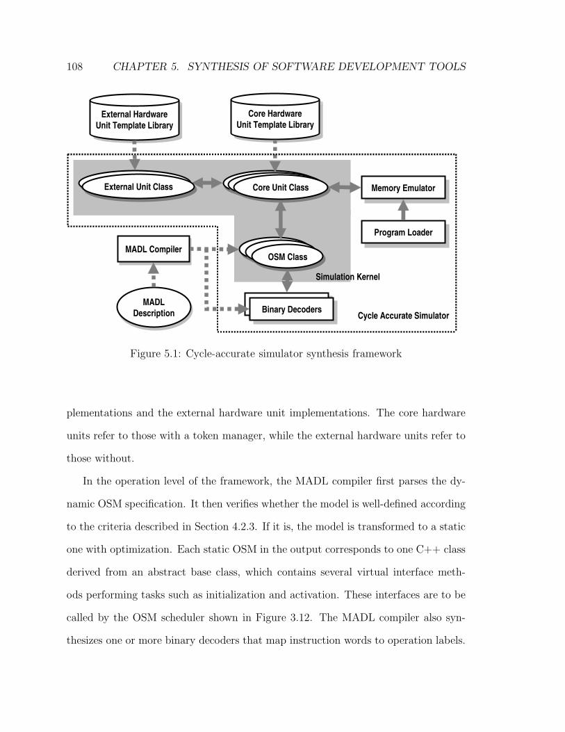
108 CHAPTER 5. SYNTHESIS OF SOFTWARE DEVELOPMENT TOOLS
Core HardwareUnit Template Library
MADLDescription
MADLDescription
MADL CompilerMADL Compiler OSM ClassOSM Class
Core Unit ClassCore Unit Class
External HardwareUnit Template Library
Binary DecodersBinary Decoders
External Unit ClassExternal Unit Class
OSM ClassOSM ClassOSM ClassOSM Class
Binary DecodersBinary Decoders
External Unit ClassExternal Unit Class Core Unit ClassCore Unit ClassCore Unit ClassCore Unit Class Memory EmulatorMemory Emulator
Program LoaderProgram Loader
Simulation Kernel
Cycle Accurate Simulator
Figure 5.1: Cycle-accurate simulator synthesis framework
plementations and the external hardware unit implementations. The core hardware
units refer to those with a token manager, while the external hardware units refer to
those without.
In the operation level of the framework, the MADL compiler first parses the dy-
namic OSM specification. It then verifies whether the model is well-defined according
to the criteria described in Section 4.2.3. If it is, the model is transformed to a static
one with optimization. Each static OSM in the output corresponds to one C++ class
derived from an abstract base class, which contains several virtual interface meth-
ods performing tasks such as initialization and activation. These interfaces are to be
called by the OSM scheduler shown in Figure 3.12. The MADL compiler also syn-
thesizes one or more binary decoders that map instruction words to operation labels.
5.2. SYNTHESIS OF THE CAS 109
These decoders are used by the OSMs for optimized state transition when decoding
is involved. The details of their use are given in Section 5.2.2.
In the hardware level of the framework, each token manager and its owner hard-
ware unit are implemented as one unified C++ class for the convenience of their state
sharing. The class contains a set of interface methods corresponding to the control
and data actions. These interfaces are to be called by the OSMs. External hard-
ware units are also implemented as C++ classes. To reuse the implementations of
the hardware units across different target processors, the commonly used units are
organized as C++ template class libraries. New hardware units can be customized by
specializing and extending the library classes or coded from scratch. As shown in the
example of Figure 4.8, annotations may be used to specify pointers to the actual core
hardware unit in the library and the template parameters. The synthesis framework
will follow these pointers to locate the corresponding implementations.
The OSM classes and the hardware unit classes are instantiated in the cycle-
accurate simulator. They are linked with the synthesized binary decoders, a memory
emulator that interprets the virtual memory address of the target processor and keeps
all its memory states, a program loader that initializes the instruction memory, and
the simulation kernel that combines the functionality of the OSM scheduler and the
clock-driven kernel. These together form a CAS in C++.
5.2.1 Simplifications of the Simulation Kernel
In general, the hardware level of the OSM model is based on the DE simulation
kernel as mentioned in Chapter 3. However, even though the OSM model brings
about significant simplification to the hardware level, DE-based simulation is not
110 CHAPTER 5. SYNTHESIS OF SOFTWARE DEVELOPMENT TOOLS
efficient in terms of simulation speed. For this reason, two simplification approaches
were used in implementing the CAS synthesis framework.
The first simplification approach involves the simulation kernel of the hardware
level of the framework. Instead of the DE kernel shown in Figure 3.12, a clock-driven
kernel is used. As mentioned in Chapter 2, the clock-driven kernel is a special case
of the DE kernel in which the only event is the clock signal. It is more efficient for
synchronous circuit modeling as the expensive event calendar of the DE kernel is no
longer needed.
The second simplification approach involves the communication mechanism among
the hardware units. Instead of using ports and channels as in normal structural
modeling approaches, the framework used interface function calls. For instance, the
communication between the instruction fetcher unit and the cache unit is implemented
as a function call by the fetcher unit to the cache unit in every clock cycle, rather
than a set of handshaking channels between the two.
As a result of the simplification approaches, each C++ class in the hardware level
contains an interface method “update on clock” to be called by the scheduler at the
clock edges. The method replaces the clock signal port. Each class also contains a
few interface methods to be called by the neighboring function units, if any. At each
clock edge, after the OSM scheduler finishes a control step, the clock-driven scheduler
activates the hardware units one after another by calling their “update on clock”
methods. A unit may call an interface of another unit for communication.
One drawback of this simplified scheme is that the activation order of the hardware
units by the clock-driven scheduler affects the behavior of the hardware units. For
instance, if the cache is activated before the instruction fetcher, its activation result
may be seen by the instruction fetcher when the fetcher is activated later at the
5.2. SYNTHESIS OF THE CAS 111
same cycle. But if the cache is activated later, its result may only be seen by the
instruction fetcher in the next cycle. Consequently, developers need to be careful in
sorting the activation order of these hardware units according to the semantics of the
microarchitecture.
This drawback is due to the use of the simplified simulation kernel. If a struc-
tural clock-driven simulation kernel or DE-based kernel is used in the hardware level,
such order-dependency problem should not exist. In fact, non-structure-based mi-
croarchitecture simulation frameworks such as SimpleScalar [4] are based on similar
simplifications and therefore have the same problem. As has been demonstrated in
Section 3.3.3, the use of the OSM model significantly simplifies the communication
between the microarchitectural units, it is much easier for OSM model developers to
sort out the activation order of the hardware units.
5.2.2 Decoding Optimization
Recall that in Section 3.3.4, an artificial token manager, Decode, is used to steer the
static OSM towards the execution path corresponding to its operation type. Each
state where such steering occurs has many fan-out edges, each of which contains
an inquiry request to the Decode manager with the token index as a tuple of the
instruction word and the index to the operation represented by the path. According
to the semantics of the OSM model, during execution the OSM tests the fan-out
edges one after another until the edge that matches the instruction word is reached.
Suppose that the matching probability is evenly distributed among the edges, the
expected testing count is one half of the number of the edges. Since there may exist
hundreds of out-going edges, the sequential testing can be very slow. In essence, this
scenario is equivalent to a long sequence of if-then-else statements in the C language.
112 CHAPTER 5. SYNTHESIS OF SOFTWARE DEVELOPMENT TOOLS
To avoid such inefficient sequential decoding, the decoding process in the OSM
is specialized in the implementation. Instead of using the Decode token manager
and having the OSM test the numerous edges, a binary decoder is used to replace
the inquiry actions on the fan-out edges. When decoding occurs, the binary decoder
evaluates the instruction word and returns the matching operation index. The OSM
then performs a table lookup with the index to locate the right destination state.
This optimization is similar to converting a sequence of if-the-else statements into a
single switch-case statement in C.
The above mentioned binary decoder is automatically synthesized with the binary
encoding information from the MADL description. Its details are given in Section 5.6.
5.2.3 Experiments
Based on the above CAS synthesis framework, case studies were performed with the
StrongARM, PLX, and Hiperion processors.
StrongARM The StrongARM core is a 5-stage pipelined implementation of the
ARM V4 architecture [1]. A sketch diagram of its microarchitecture is shown in
Figure 5.2. Its MADL-based model implements all user-level instructions. It also
includes a coprocessor-instruction-based interface for communicating with input and
output devices. The model is developed together with MADL and the CAS synthesis
framework. These altogether took about nine man-months. Software applications
can access the device interface through using the coprocessor-instructions of the ARM
instruction set. The synthesized CAS can run benchmarks built by gcc [21].
Though generally viewed as a RISC processor, the ARM ISA contains some CISC
features such as the load-multiple operation ldm. A ldm can load 0 to 15 register
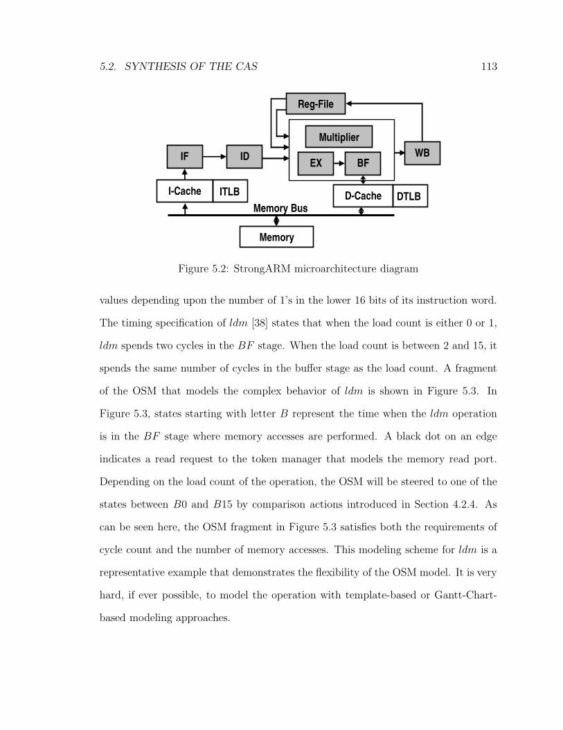
5.2. SYNTHESIS OF THE CAS 113
IF ID EX BFWB
I-Cache D-Cache
Memory
Memory Bus
Reg-File
ITLB DTLB
Multiplier
Figure 5.2: StrongARM microarchitecture diagram
values depending upon the number of 1’s in the lower 16 bits of its instruction word.
The timing specification of ldm [38] states that when the load count is either 0 or 1,
ldm spends two cycles in the BF stage. When the load count is between 2 and 15, it
spends the same number of cycles in the buffer stage as the load count. A fragment
of the OSM that models the complex behavior of ldm is shown in Figure 5.3. In
Figure 5.3, states starting with letter B represent the time when the ldm operation
is in the BF stage where memory accesses are performed. A black dot on an edge
indicates a read request to the token manager that models the memory read port.
Depending on the load count of the operation, the OSM will be steered to one of the
states between B0 and B15 by comparison actions introduced in Section 4.2.4. As
can be seen here, the OSM fragment in Figure 5.3 satisfies both the requirements of
cycle count and the number of memory accesses. This modeling scheme for ldm is a
representative example that demonstrates the flexibility of the OSM model. It is very
hard, if ever possible, to model the operation with template-based or Gantt-Chart-
based modeling approaches.

114 CHAPTER 5. SYNTHESIS OF SOFTWARE DEVELOPMENT TOOLS
EX B15 B14 B13
B1 BY WB
B2
B0
BX
count==2, …count==2, …
count==1, …count==1, …
count==0, …count==0, …
Figure 5.3: OSM fragment modeling ldm
PLX The PLX processor [46] is a research architecture implemented by the PALMS
group in Princeton University. It features a subword-parallel ISA containing more
than 200 integer and floating-point instructions. A standard 5-stage pipelined imple-
mentation with one level of data and instruction caches is used in this case study. Its
MADL model were mainly developed by its designers in six man-weeks. The support
of various integer and floating-point data types by MADL makes it convenient to
implement the subword-parallel semantics of PLX.
Hiperion Hiperion is a 16-bit VLIW DSP with an irregular ISA. Its instruction
encoding is optimized mainly for code size and therefore is not fully orthogonal. The
development of its MADL model was performed in collaboration with Subramanian
Rajagopalan and was completed in about three weeks. The model implements a sub-
set of the ISA that is supported by a C language compiler customized by Subramanian
for the processor. The microarchitecture involves an 8-stage pipeline. The memory
hierarchy is flat with no caches used. As the Hiperion processor features variable-
length instruction width, the instruction fetch unit is different from the previous two
models. An OSM can send more than one read request to the token manager for its
instruction word.
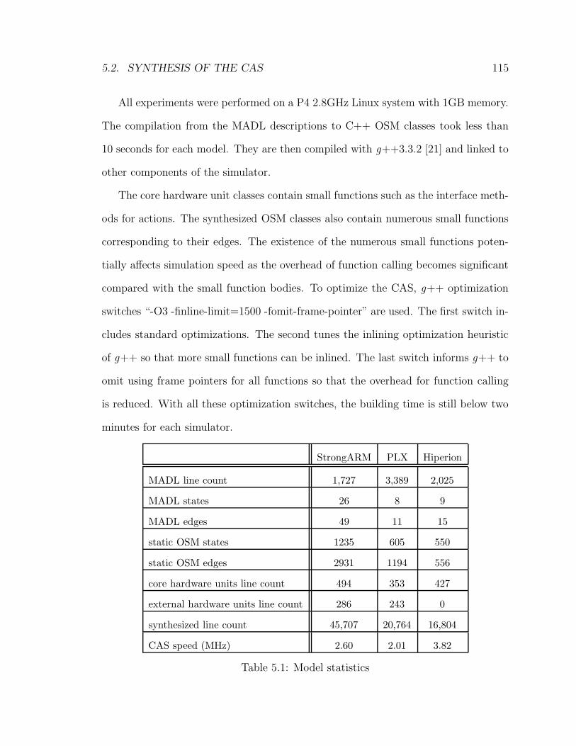
5.2. SYNTHESIS OF THE CAS 115
All experiments were performed on a P4 2.8GHz Linux system with 1GB memory.
The compilation from the MADL descriptions to C++ OSM classes took less than
10 seconds for each model. They are then compiled with g++3.3.2 [21] and linked to
other components of the simulator.
The core hardware unit classes contain small functions such as the interface meth-
ods for actions. The synthesized OSM classes also contain numerous small functions
corresponding to their edges. The existence of the numerous small functions poten-
tially affects simulation speed as the overhead of function calling becomes significant
compared with the small function bodies. To optimize the CAS, g++ optimization
switches “-O3 -finline-limit=1500 -fomit-frame-pointer” are used. The first switch in-
cludes standard optimizations. The second tunes the inlining optimization heuristic
of g++ so that more small functions can be inlined. The last switch informs g++ to
omit using frame pointers for all functions so that the overhead for function calling
is reduced. With all these optimization switches, the building time is still below two
minutes for each simulator.
StrongARM PLX Hiperion
MADL line count 1,727 3,389 2,025
MADL states 26 8 9
MADL edges 49 11 15
static OSM states 1235 605 550
static OSM edges 2931 1194 556
core hardware units line count 494 353 427
external hardware units line count 286 243 0
synthesized line count 45,707 20,764 16,804
CAS speed (MHz) 2.60 2.01 3.82
Table 5.1: Model statistics
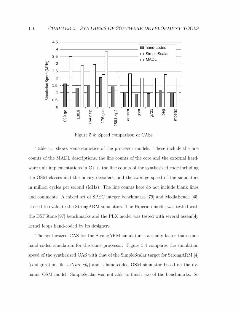
116 CHAPTER 5. SYNTHESIS OF SOFTWARE DEVELOPMENT TOOLS
0
0.5
1
1.5
2
2.5
3
3.5
4
4.5
099.
go
130.
li
164.
gzip
176.
gcc
256.
bzip
2
adpc
m
gsm
g721
jpeg
mpe
g2
hand-coded
SimpleScalar MADL
Sim
ulat
ion
Spee
d (M
Hz)
Figure 5.4: Speed comparison of CASs
Table 5.1 shows some statistics of the processor models. These include the line
counts of the MADL descriptions, the line counts of the core and the external hard-
ware unit implementations in C++, the line counts of the synthesized code including
the OSM classes and the binary decoders, and the average speed of the simulators
in million cycles per second (MHz). The line counts here do not include blank lines
and comments. A mixed set of SPEC integer benchmarks [79] and MediaBench [45]
is used to evaluate the StrongARM simulators. The Hiperion model was tested with
the DSPStone [97] benchmarks and the PLX model was tested with several assembly
kernel loops hand-coded by its designers.
The synthesized CAS for the StrongARM simulator is actually faster than some
hand-coded simulators for the same processor. Figure 5.4 compares the simulation
speed of the synthesized CAS with that of the SimpleScalar target for StrongARM [4]
(configuration file sa1core.cfg) and a hand-coded OSM simulator based on the dy-
namic OSM model. SimpleScalar was not able to finish two of the benchmarks. So
5.2. SYNTHESIS OF THE CAS 117
their corresponding data are missing in the figure. The results show that the synthe-
sized simulator runs at twice the speed of the hand-coded simulators on average. The
main reason for this difference is that when coding by hand, programmers commonly
have to trade code speed for code simplicity. For instance, in the hand-coded OSM
simulators, the dynamic OSM model is used as it is much more convenient to specify
the state diagram of a dynamic OSM. This choice greatly simplifies the implementa-
tion, but at the significant cost of the dynamic binding overhead. In contrast, coding
complexity is not a concern for synthesized code. As long as the building time of
g++ is in control, the fastest option is always favored. Therefore, the synthesized
code can afford to be more specialized towards faster simulation speed. SimpleScalar
has some speed disadvantage due to its run-time configurability, viz., some architec-
ture parameters can be specified at run-time, such as cache size, issue width, etc. But
it is unlikely that its effect is significant.
The MADL-based model is calibrated against an iPAQ-3650 PDA [12] containing a
StrongARM processor with small kernel loops designed to detect the latencies induced
by different operation sequences. It is then tested with the standard benchmarks.
Table 5.2 shows the execution time of the benchmarks on iPAQ and the simulated
time. The remaining timing mismatch can be attributed to the resolution of the
time utility used to measure the iPAQ execution time, the emulation of the operation
system in the CAS1, and most importantly, the inexact memory subsystem model
due to the lack of document for hardware details.
The MADL-based CAS synthesis approach also features high modeling produc-
tivity. Source code line count is used as a rough measure to compare the productivity
between different implementations. In the MADL case, the total line count for the
1The CAS interprets Linux system calls, but does not actually simulate the whole operatingsystem.
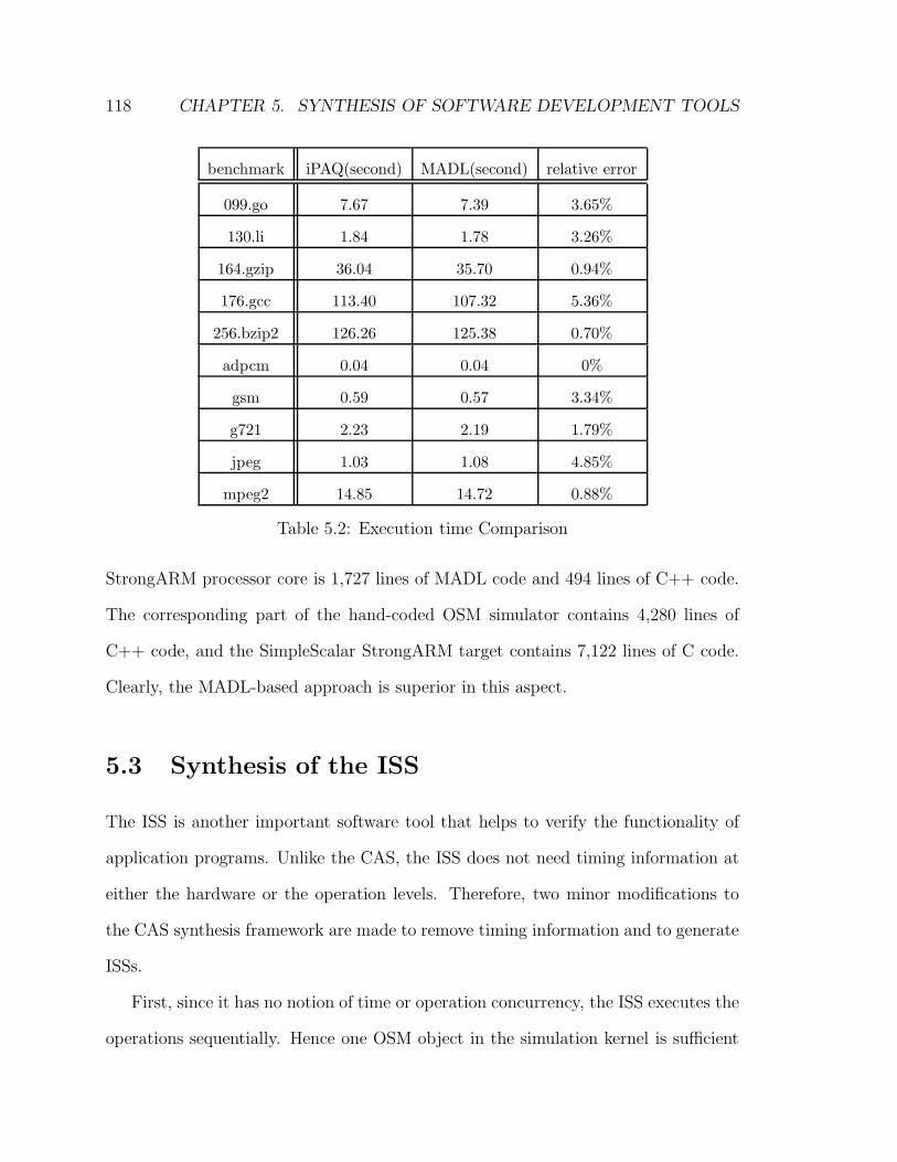
118 CHAPTER 5. SYNTHESIS OF SOFTWARE DEVELOPMENT TOOLS
benchmark iPAQ(second) MADL(second) relative error
099.go 7.67 7.39 3.65%
130.li 1.84 1.78 3.26%
164.gzip 36.04 35.70 0.94%
176.gcc 113.40 107.32 5.36%
256.bzip2 126.26 125.38 0.70%
adpcm 0.04 0.04 0%
gsm 0.59 0.57 3.34%
g721 2.23 2.19 1.79%
jpeg 1.03 1.08 4.85%
mpeg2 14.85 14.72 0.88%
Table 5.2: Execution time Comparison
StrongARM processor core is 1,727 lines of MADL code and 494 lines of C++ code.
The corresponding part of the hand-coded OSM simulator contains 4,280 lines of
C++ code, and the SimpleScalar StrongARM target contains 7,122 lines of C code.
Clearly, the MADL-based approach is superior in this aspect.
5.3 Synthesis of the ISS
The ISS is another important software tool that helps to verify the functionality of
application programs. Unlike the CAS, the ISS does not need timing information at
either the hardware or the operation levels. Therefore, two minor modifications to
the CAS synthesis framework are made to remove timing information and to generate
ISSs.
First, since it has no notion of time or operation concurrency, the ISS executes the
operations sequentially. Hence one OSM object in the simulation kernel is sufficient
5.3. SYNTHESIS OF THE ISS 119
to model the sequential operation stream. The simulation kernel becomes a simple
loop that iteratively activates the OSM object. In each iteration, the OSM executes
the complete semantics of one operation from its fetch to its retirement without in-
terruption. In other words, the OSM acts as a procedure, not as a user-level “thread”
which executes and yields at each control step in the CAS.
The second modification involves the implementation of the hardware layer. The
token managers are simplified by removing all timing or concurrency related control
semantics. For instance, since structural hazards are not a concern in the ISS, the
token managers can always approve the allocation requests from the OSM. Similarly,
the data forwarding mechanism can be omitted as data hazards are not an issue for
the ISS either. The memory hierarchy can also be simplified as caches are no longer
needed. With the simplified hardware level, the same MADL description used for
CAS generation can be used to generate ISSs.
5.3.1 Procedure Generation
For the first modification, a simple transformation is used to convert a static OSM to
a procedure. The transformation is illustrated in Figure 5.5. Figure 5.5(a) represents
the state diagram, while Figure 5.5(b) is the result of the transformation. During
the transformation, each edge of the state diagram is translated to a condition block
and an execution block. The condition block tests the state transition condition as a
normal OSM does, and the execution block commits the actions and the computations
on the edge. Each state of the state diagram is translated to the same number of
labels as its outgoing edges. These condition blocks and the labels form a ladder of
if-then-else statements, with the top-most block corresponding to the edge with the
highest priority. In this example, state D has two outgoing edges, therefore, it is
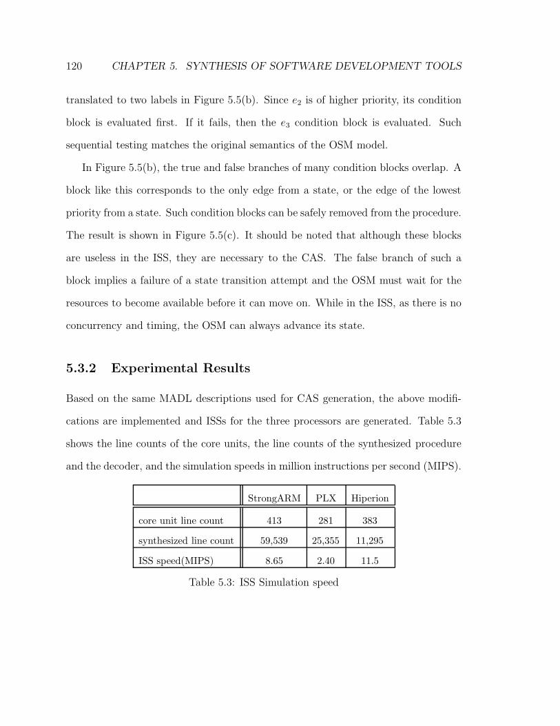
120 CHAPTER 5. SYNTHESIS OF SOFTWARE DEVELOPMENT TOOLS
translated to two labels in Figure 5.5(b). Since e2 is of higher priority, its condition
block is evaluated first. If it fails, then the e3 condition block is evaluated. Such
sequential testing matches the original semantics of the OSM model.
In Figure 5.5(b), the true and false branches of many condition blocks overlap. A
block like this corresponds to the only edge from a state, or the edge of the lowest
priority from a state. Such condition blocks can be safely removed from the procedure.
The result is shown in Figure 5.5(c). It should be noted that although these blocks
are useless in the ISS, they are necessary to the CAS. The false branch of such a
block implies a failure of a state transition attempt and the OSM must wait for the
resources to become available before it can move on. While in the ISS, as there is no
concurrency and timing, the OSM can always advance its state.
5.3.2 Experimental Results
Based on the same MADL descriptions used for CAS generation, the above modifi-
cations are implemented and ISSs for the three processors are generated. Table 5.3
shows the line counts of the core units, the line counts of the synthesized procedure
and the decoder, and the simulation speeds in million instructions per second (MIPS).
StrongARM PLX Hiperion
core unit line count 413 281 383
synthesized line count 59,539 25,355 11,295
ISS speed(MIPS) 8.65 2.40 11.5
Table 5.3: ISS Simulation speed
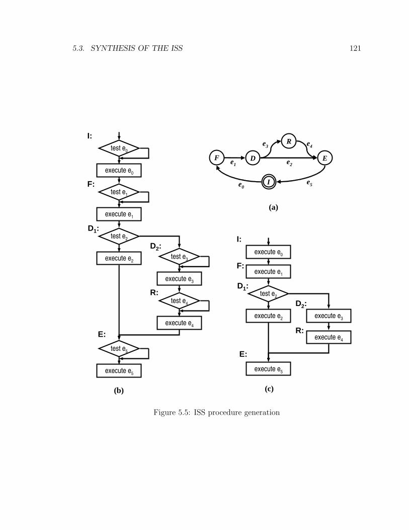
5.3. SYNTHESIS OF THE ISS 121
R
ED
Ie0
e2e1
e3 e4
e5
Ftest e0
execute e0
test e1
execute e1
test e2
execute e2test e3
execute e3
test e4
execute e4
test e5
execute e5
I:
F:
R:
D1:
E:
D2: execute e0
execute e1
test e2
execute e2 execute e3
execute e4
execute e5
I:
F:
R:
D1:
E:
D2:
(a)
(b) (c)
Figure 5.5: ISS procedure generation
122 CHAPTER 5. SYNTHESIS OF SOFTWARE DEVELOPMENT TOOLS
Currently the speeds of the synthesized ISSs are slower than those hand-coded
ones. In the StrongARM case, the synthesized simulator runs at about 27% the
speed of the hand-coded simulator from [66]. There are two main reasons for the
discrepancy. First, the synthesized simulator reads and writes register and memory
data values through the token transaction protocol. As mentioned in Section 3.3, to
write a data value, a token should be allocated first. The data value is written to
the token through the write action. Similarly, reading a data value also requires first
allocating or inquiring about the token. Compared with direct variable references in
the hand-coded simulator, the token-based data communication scheme contains one
extra level of indirection and is therefore less efficient. Such overhead also exists in
synthesized CASs, but they are less sensitive to the overhead as data communication
constitutes only a much smaller fraction of their execution time. Second, since the
same MADL description for CAS synthesis is used for ISS generation, the resulting
ISS evaluates operation semantics following the state diagram designed for cycle-
accurate simulation. For each operation, it undergoes the normal stages of fetching,
decoding, evaluation, and result write-back. In contrast, the hand-coded simulator
does not have to follow these stages and can thereby benefit from some processor-
specific optimizations. In the StrongARM case, the hand-coded simulator evaluates
the predicate operand of an operation prior to fully decoding it. If the predicate
operand is false, the operation will be skipped and its decoding/evaluation time can
be saved. Such early evaluation of the predicate operand is not possible in the CAS as
it violates timing constraints. Therefore the synthesized ISS cannot benefit from this
type of optimization. In addition to the above two, a relatively small slowdown factor
for the synthesized simulators is their use of a bit-true integer library to represent all
data values. While in hand-coded simulators, native data types are used.
5.4. SYNTHESIS OF THE DISASSEMBLER 123
The speed of the ISSs can be improved by using different MADL descriptions from
those used to generate CASs. However, it is probably more valuable to synthesize
both types of simulators from the same description as it improves productivity and
ensures consistency. Optimization opportunities need to be explored to improve the
speed of the ISSs.
The ISS synthesis framework is limited in that it does not handle delay slots.
Two types of delay slots commonly exist in processors, branch delay slots and data
delay slots. Branch delay slots postpone the update of the program counter till one
or several instructions after the taken branch operation. It appears in instruction
sets such as the SPARC ISA [78]. To accommodate branch delay slots, minor manual
intervention is necessary to intervene the update of the program counter. The data
delay slot refers to the situation when an operation updates its destination register
value after its successor operation begins to execute. So the successor is not affected
by the predecessor and still reads the old register value. Such type of delay slots often
appear in processors without data interlocking mechanism, such as the TMS320C6000
series DSPs [86]. The modeling of such delay slots requires operation level concurrency
support in the simulator. Therefore the above mentioned ISS cannot handle this. A
CAS with a simplified hardware level can be used as an ISS in such a case.
5.4 Synthesis of the Disassembler
As mentioned in Chapter 4, assembly syntax chunks can be specified in the “SYN-
TAX” subsections of the syntax operations. The chunks from an expansion of the
AND-OR graph can be assembled together to form an assembly template for the type
of operations matching the expansion. The template is the concatenation of a set of
124 CHAPTER 5. SYNTHESIS OF SOFTWARE DEVELOPMENT TOOLS
string literals and variables. The string literals represent the operation name, the
punctuations and spaces in the assembly; while the variables represent the operand
fields. For the example description in Figure 4.5, the assembly template for the ex-
pansion involving “alu”, “add”, and “imm” is the concatenation of “add R”, rs1,
v imm, “R”, and rd.
Given an instruction word, its matching expansion and the assembly template can
be located as a result of decoding. The variables corresponding to operand fields can
be extracted from the instruction word and filled into the template. The assembly
output of the operation is then obtained.
The implementation of the disassembler is straightforward as most of its com-
ponents are available in the CAS and the ISS synthesis framework. Therefore, it is
simply integrated in the simulation framework as a utility. It can be used to print
out execution traces of the simulators for debugging of the simulated programs.
In principle, the inverse of the disassembler – the assembler – can also be synthe-
sized based on the assembly templates. It is not implemented in this work as it is not
directly useful to the simulators and it adds little more value than the disassembler
in demonstrating the effectiveness of MADL.
5.5 Extraction of the Reservation Table
The instruction scheduler is an important component of an HLL compiler as it helps
reduce the execution time of a program by increasing execution parallelism of a pro-
gram and hiding instruction latencies. This is especially true for embedded processors
as many of them are statically scheduled and fully depend on the compiler for best
performance.
5.5. EXTRACTION OF THE RESERVATION TABLE 125
One popular class of instruction schedulers is the list scheduler. A list scheduler
maintains a two dimensional scheduling table. The rows of the table represent all
resources and the columns represent cycle time. The resource consumption of an
operation is modeled as one or more reservation tables. A reservation table is also a
two dimensional tables specifying the usage of resources at different time slots. The
list scheduling algorithm packs the reservation tables of the operations in a program
into the scheduling table so as to minimize the total scheduling length while preserving
data and control dependency of the program. The packing process is similar to playing
the Tetris computer game. The list scheduler offers fast scheduling speed as well as
good retargetability. Hence it is among the most widely used types of schedulers.
This section describes how to extract reservation tables from MADL descriptions for
the use of the list scheduler.
In order to build a reservation table, the scheduler needs to obtain information of
the physical and artificial resources of the processor (such as issue slots and functional
units), possible execution paths for each operation, and resource usages of each oper-
ation describing the time slots when different resources are used. The information is
all contained in the OSM model, but often mixed with other information irrelevant
to the instruction scheduler. This makes it difficult to extract the information useful
to the scheduler. For instance, as resources are modeled as tokens in the OSM model,
not all tokens are related to scheduling. Therefore some hints need to be provided to
highlight those resources related to scheduling. Also the instruction scheduler may
not understand the complete details of an executable model and simplification is of-
ten needed. For example, the instruction scheduler assumes that each operation has
fixed latency, even though in real hardware variable latency is common. Compiler
developers must simplify such variable latency by providing the scheduler with an
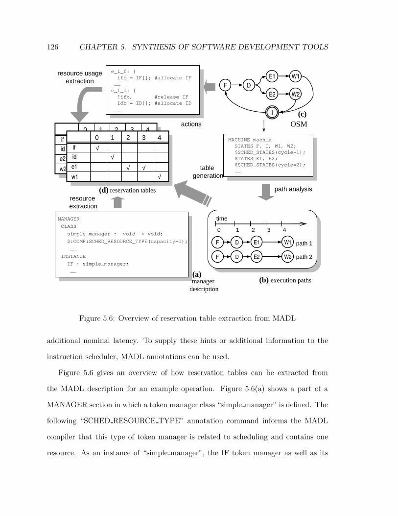
126 CHAPTER 5. SYNTHESIS OF SOFTWARE DEVELOPMENT TOOLS
ifide2
w2
0 1 2 3 4
√√
√ √√
ifide2
w2
0 1 2 3 4
√√
√ √√
F DE1
E2
W1
W2
I
F D E1 W1
F D E2 W2
path analysis
ifide1
w1
0 1 2 3 4
√√
√ √√
ifide1
w1
0 1 2 3 4
√√
√ √√
path 1
path 2
time
0 1 2 3 4
table generation
MANAGER
CLASS
simple_manager : void -> void;
$:COMP:SCHED_RESOURCE_TYPE(capacity=1);
……
INSTANCE
IF : simple_manager;
……
MANAGER
CLASS
simple_manager : void -> void;
$:COMP:SCHED_RESOURCE_TYPE(capacity=1);
……
INSTANCE
IF : simple_manager;
……
resource extraction
resource usageextraction
OSM
e_i_f: {ifb = IF[]; #allocate IF……e_f_d: {!ifb, #release IFidb = ID[]; #allocate ID
……
e_i_f: {ifb = IF[]; #allocate IF……e_f_d: {!ifb, #release IFidb = ID[]; #allocate ID
……
actions
manager description
reservation tables
(a)
(c)
(b) execution paths
(d)
MACHINE mach_aSTATES F, D, W1, W2;$SCHED_STATES(cycle=1);STATES E1, E2;$SCHED_STATES(cycle=2);……
MACHINE mach_aSTATES F, D, W1, W2;$SCHED_STATES(cycle=1);STATES E1, E2;$SCHED_STATES(cycle=2);……
Figure 5.6: Overview of reservation table extraction from MADL
additional nominal latency. To supply these hints or additional information to the
instruction scheduler, MADL annotations can be used.
Figure 5.6 gives an overview of how reservation tables can be extracted from
the MADL description for an example operation. Figure 5.6(a) shows a part of a
MANAGER section in which a token manager class “simple manager” is defined. The
following “SCHED RESOURCE TYPE” annotation command informs the MADL
compiler that this type of token manager is related to scheduling and contains one
resource. As an instance of “simple manager”, the IF token manager as well as its
5.5. EXTRACTION OF THE RESERVATION TABLE 127
token will be taken into account for resource extraction. All other physical resources
are similarly defined by annotations on their respective manager classes.
Figure 5.6(c) shows the state diagram for the example operation. The state di-
agram is specified in the MACHINE section in the MADL description. Some state
declarations in the machine section are followed by the “SCHED STATES” annota-
tion commands. These commands notify the extraction tool that these states are
relevant to the scheduling process. The tool analyzes the connectivity of the state
diagram and finds the longest paths that are solely composed of such relevant states.
These paths are regarded as the alternative execution paths of the operation and the
nominal execution latencies along the paths are obtained according to the “cycle”
argument of the annotation commands. The results are illustrated in Figure 5.6(b).
Moreover, by analyzing the actions on the edges of the execution paths the extrac-
tion tool can determine the resources used at each state. In this example, when the
state machine proceeds from state I to F, it allocates the token of the IF manager.
Therefore it can be deduced that the IF token is used by the state machine at state F.
The token is given up when the state machine proceeds to state D and commits the
release action. Hence by examining all the allocate, release, and discard actions along
all execution paths, the MADL compiler can obtain the resource usage information
of the operation.
Finally, with all the information extracted above, the reservation tables can be
constructed as shown in Figure 5.6(d). Each reservation table corresponds to one
execution path in Figure 5.6(b).
The MADL specifications for StrongARM and Hiperion in Section 5.2 are aug-
mented with annotations needed for reservation table extraction. From the core and
the annotation layers of both descriptions, an extraction tool as a post-processor of
128 CHAPTER 5. SYNTHESIS OF SOFTWARE DEVELOPMENT TOOLS
the MADL compiler was developed to obtain reservation tables. For the StrongARM
model, 6 physical resources and 548 reservation tables were generated, whereas, 12
resources and 164 reservation tables were generated for the Hiperion model.
5.6 Synthesis of the Binary Decoder
In Section 5.2, a binary decoder is used to optimize the steering of the OSM. The
same decoder is also used in the ISS and the disassembler. This section describes how
the decoder is synthesized.
A binary decoder maps instruction words to matching operation labels. The
matching can be evaluated by comparing the instruction word with the encoding pat-
terns of the operations, which can be extracted from MADL descriptions in the same
way as assembly templates. For the example description in Figure 4.5, the encoding
pattern for the expansion involving “alu”, “add”, and “imm” syntax operations is the
concatenation of “000000”, rd, rs1, “1”, and vimm. An instruction word “000000 111
001 1 010” matches the pattern since there is no conflict in a bit-wise comparison of
the two. The extracted patterns are used as the input to the binary decoder synthesis
algorithm.
In general, software decoding is sequential and control flow intensive. This is in
contrast to hardware-based decoding where multiple logic expressions can be evalu-
ated concurrently. Therefore, the speed of a software binary decoder can be very slow
if an inefficient algorithm is used. Depending on the portion of execution time spent
in decoding, the decoder may become a performance bottleneck for speed-critical soft-
ware tools such as instruction set simulators (ISSs). According to the results reported
5.6. SYNTHESIS OF THE BINARY DECODER 129
by other researchers [57], a slow decoder can affect the simulation speed of the ISSs
by a factor of two to four. An efficient binary decoder is thus highly desirable.
5.6.1 Related Work
Efficient hand-coded binary decoders for general-purpose processors can be found
in popular tools such as the GNU debugger [20]. Its typical decoding scheme is to
extract the main opcode field of the instruction and then perform a multi-way branch
based on its value. After the main opcode is decoded, the sub-opcode fields can be
handled in a similar way. The hand-coded decoders require human intelligence that
is not available in automatic decoder synthesis. For complex and irregular instruction
sets, it is an error-prone task for humans to find a good solution.
A simple binary decoder synthesis scheme is described in [27]. The generated
decoder sequentially matches the input bit string with all possible instruction pat-
terns that were extracted from a description in the architecture description language
ISDL [26]. The execution time of such a decoding scheme is linear in the number of
instructions of the instruction set. Since a typical instruction set contains more than
100 instructions, the sequential decoding scheme can be very slow.
In [89], a decision-tree-based decoding scheme is described. Each internal node of
the decision tree tests a few bits of the input bit string and makes a multi-way branch
to the matching child node. The process iterates until a leaf node is reached where
the instruction can be unambiguously classified. The decoder synthesis algorithm is
deterministic in that the synthesized decoding tree is completely determined by the
input instruction set specification. It generates decoders with efficiency comparable to
that of hand-coded decoders in the reported cases. A known problem of the algorithm
is that it will fail on certain instruction pattern combinations. For instance, the set
130 CHAPTER 5. SYNTHESIS OF SOFTWARE DEVELOPMENT TOOLS
of encoding patterns “-10”, “00-”, and “1-1” contains no bit field that is either ‘0’ or
‘1’ for all three. Since the algorithm requires such a bit field as the starting point of
decoding, it simply gets stuck in this case. The author assumed that such a situation
will not appear in processor designs. The assumption is not fully justified since such
a situation may occur in ASIP designs where irregular encoding may be preferable
due to code size considerations.
The New Jersey Machine-Code Toolkit [73] is capable of synthesizing binary de-
coders from machine specifications of a special format. In order to generate an efficient
binary decoder, the instruction word must be divided into individual fields and the
instruction patterns must be grouped as tables in the specification. In a retargetable
software tool development environment where a general architecture description lan-
guage is used, it is a non-trivial task to derive such a well-organized specification,
especially when the instruction set is irregular.
The efficiency of binary decoding in ISS is addressed from a different angle in [57].
The proposed technique exploits the locality of the program under simulation by
caching the decoding results for reuse. When the cache hit rate is high, decoder ef-
ficiency becomes less of a problem. However, caching the decoding results consumes
a large portion of the precious data cache and therefore negatively impacts the sim-
ulation speed. Furthermore, the decoding cache hit ratio is subject to the locality
characteristics of the program being simulated and therefore its performance cannot
be guaranteed.
The problem of decoder construction is closely related to the long studied multi-
discipline field of decision tree construction from data [52, 56]. Specifically, the prob-
lem of binary decoding is very similar to the problem of identification key construc-
tion [63], which has been studied in the fields of systematic biology, pattern recog-
5.6. SYNTHESIS OF THE BINARY DECODER 131
nition, fault diagnostics, etc. However, due to the different context, objective, and
problem scale, no existing solution can be directly borrowed from these fields. To
the author’s knowledge, binary decoder construction has not been discussed in the
decision tree construction field.
5.6.2 Problem Formulation
The task of a binary decoder is to find the matching operation type for a bit string.
The design of an efficient decoder is an optimization problem. This section formulates
the problem.
Definitions
A bit pattern is defined as p∈{0, 1,−}n, where 0 and 1 are binary values and “−”
stands for a don’t-care value. A bit string s∈Bn (B = {0, 1}) matches a pattern p if
and only if ∀0≤i≤n, either s[i] = p[i] or p[i] = −. It is denoted as s∈p if s matches p.
Each operation type is represented by one or more decoding entries in the triple
form of (p, l, λ), where p is a bit pattern of length n, l∈L a classification label, and λ∈R
the probability that a bit string will match p. An instruction set can be represented by
a set of such decoding entries. As pointed out in [89], for a variable length instruction
set, the short patterns can be padded with “−”s so that all patterns are of the same
length. A null entry is a special type of decoding entry. Its classification label is
empty. It is used to represent an invalid pattern of the instruction set.
Given a set of decoding entries E, the task of a binary decoder d : Bn 7→L is to
map a bit string s to the classification label of decoding entry (p, l, λ)∈E so that s∈p.
The capacity of E is defined as the total number of unique bit strings that can match
a pattern in E. The set E is said to be well-formed if there exists no bit string that
132 CHAPTER 5. SYNTHESIS OF SOFTWARE DEVELOPMENT TOOLS
(000--, l1, 0.25)(001--, l2, 0.25)(01---, l3, 0.25)(1----, l4, 0.25)
(001--, l1, 0.25)(000--, l2, 0.25)(-1---, l3, 0.25)(1----, l4, 0.25)
(a) Well-formed (b) Not well-formed
Figure 5.7: Example pattern sets
matches more than one entry. Figure 5.7(a) shows a well-formed pattern set example,
while Figure 5.7(b) shows a not-well-formed pattern set, in which case a bit string
“11000” matches both the third and the fourth entry.
In logic synthesis terminology, a pattern specifies a product term in the space of
Bn. Well-formedness can be verified by checking that the products of all pattern pairs
are zero.
Decoding Tree
Decoding is a search process. Common searching algorithms, including hashing, can
all be represented by search trees [43]. The problem of decoder construction is there-
fore equivalent to the construction of a min-cost search tree.
A decoding tree (V, E) is similar to a decision tree in [89]. The node set V is the
union of the set of terminal nodes D and the set of inner nodes N . Each terminal
node is labeled with either a decoding entry or a null entry. Each inner node v∈N
is labeled with a decision function fv : Bn 7→Z, where Z is the set of integers. Each
possible evaluation result of fv corresponds to an outgoing edge of v, which is labeled
with the result value.
The decoding process starts from the root node. It iteratively evaluates the de-
cision function of the current node with the input bit string s as the argument, and
5.6. SYNTHESIS OF THE BINARY DECODER 133
10
(01---,l3,0.25)
(1----,l4,0.25)
0 1
(001--,l2,0.25)(000--,l1,0.25)
0 1
“01101”
p[4]==1
p[3]==1
p[2]==1
Figure 5.8: Example decoding tree
descends along the edge labeled with the same value as the evaluation result. The
process repeats until a terminal node is reached. If the node is a decoding entry, then
its classification label is the decoding result; if the node is a null entry, then a decoding
error is reported. A decoding error occurs when s matches no given pattern. Given a
decoding tree, the decoding height H(s) is defined as the number of edges from the
root node to the matching terminal node. Figure 5.8 shows a possible decoding tree
for the decoding entry set of Figure 5.7. The decoding path for bit string “01101”
has a height of 2.
The construction of a decoder involves selecting the tree structure as well as the
set of decision functions for the inner nodes.
Cost Modeling
To evaluate the execution efficiency of a decoder, the average execution time of the
decision function is used as the decoding cost. However, the actual time is known
until the entire decoder is constructed, compiled, and tested, which is impractical
if the construction process involves the evaluation of a huge number of candidate
decoders. Therefore, it is necessary to model the execution time at a higher level.
134 CHAPTER 5. SYNTHESIS OF SOFTWARE DEVELOPMENT TOOLS
Suppose that the execution time of each decision function in the decoding tree is
constant. The average decoding height can be taken as a measure of decoding time,
which is defined as
Havg =1
K
K∑
i=1
H(si) =∑
i
λi·D(ei), (5.1)
where K is the total number of decoded bit strings, and D(ei) is the path length from
the root to the terminal node with the decoding entry ei.
Note that the execution time of a modern microprocessor is affected not only by
the length of the execution trace but also by its memory usage. So in order for the
above estimation to be reasonably accurate, it must be ensured that the synthesized
decoder uses only a limited amount of memory. If memory usage is unlimited, the
smallest decoding height can always be achieved by a lookup table of size 2n.
In summary, the decoder construction problem can be stated as below: from a
well-formed decoding entry set E, construct a decoding tree dmin so that dmin has the
minimum average decoding height under given memory usage constraints. The input
of such a problem requires the least amount of knowledge about operation encoding
formats and can be easily obtained from any form of machine description containing
encoding information.
5.6.3 Decision function
In general, the decision functions can be constructed from arbitrary arithmetic or
logic operators and their combinations. So there exist a technically infinite number
of possible candidates for decision functions.2 To simplify the selection of decision
functions, only two classes of simple decision functions as shown below are allowed.
2The actual number of functions with an n-bit input and m possible outcomes is m2n
.
5.6. SYNTHESIS OF THE BINARY DECODER 135
1. Pattern decoding
A pattern decoding function tries to match the bit string s with a pre-specified
pattern. The function returns 1 if the two match and 0 otherwise. Since the
function has only two possible results, a node with a pattern decoding function
always has two children.
2. Table decoding
A table decoding function extracts m contiguous bits from the bit string as its
result. Such a function has 2m possible outcomes. Therefore a node with a
table decoding function has 2m children.
The two classes are chosen since they are commonly used in hand-coded decoders.
They can be implemented efficiently as single C statements if the bit string of size n
can fit into a built-in data type of C. Such efficiency is desirable since it keeps the
decoder small and fast, and the similar costs of the two types of functions validate
the execution time assumption for Equation (5.1).
The contiguity constraint for table decoding keeps the decoding function simple.
It also helps to limit the number of table decoding functions to n(n + 1)/2. On the
other hand, if non-contiguous bits are allowed, there would be 2n − 1 total table
functions, which is too large to handle when n grows beyond 16. The constraint is
not a serious efficiency problem in practice since table decoding is most useful for
decoding the opcode fields of an instruction set, which are contiguous in most cases.
5.6.4 Division of Decoding Entry Set
At the start of the decoding process, all decoding entries are viewed as possible
decoding outcomes since there exists a path from the root node to any leaf node.
136 CHAPTER 5. SYNTHESIS OF SOFTWARE DEVELOPMENT TOOLS
Once the decision function of the root node is evaluated, the decoder can descend
along the edge corresponding to the evaluation result to one child-node v. At this
point, the possible decoding outcomes contain only the leaf nodes of the sub-tree
under v, which constitute a subset of the entire decoding entry set. In other words,
the evaluation of a decision function f divides a decoding entry set into a set of
smaller ones by “revealing” information from the bit string. Such division provides
for a means to divide and conquer the decoding problem.
To understand how a decision function f divides a decoding entry set E into {Ei},
consider two cases for each entry (p, l, λ)∈E,
1. If ∀s∈p, f(s) = i, then add (p, l, λ) to set Ei.
2. If bit strings matching p evaluate to several results, then split the entry to
a smallest set {(pi, l, λi)} so that ∀s∈pi, f(s) is a constant ci, and ∪pi = p,
∑
λi = λ with λi’s linearly proportional to the probabilities that s matches
pi’s. Add entry (pi, l, λi) to Eci.
The second case above involves splitting decoding entries, which is one major
difference between the proposed algorithm and the one in [89]. Figure 5.9(a) shows
a division example of a table decoding function that extracts the left-most two bits.
Figure 5.9(b) shows one possible decoding tree constructed from the division. The
average height of the tree is 1.5 in this case. In comparison, based on the algorithm
of [89] in which splitting is not allowed, Figure 5.8 is the only possible decoding tree
with an average decoding height of 2. Clearly, splitting enables the trade-off of tree
width with tree height and allows for faster decoding. Moreover, splitting allows
the proposed algorithm to handle pattern sets that are not allowed in the algorithm
in [89]. For the aforementioned encoding pattern set “-10”, “00-”, and “1-1”, the
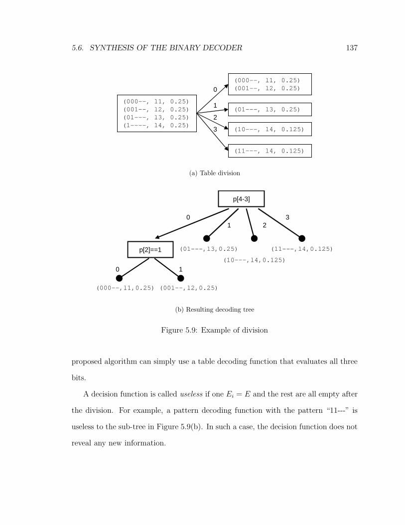
5.6. SYNTHESIS OF THE BINARY DECODER 137
(000--, l1, 0.25) (001--, l2, 0.25) (01---, l3, 0.25) (1----, l4, 0.25)
(000--, l1, 0.25) (001--, l2, 0.25)
(01---, l3, 0.25)
(10---, l4, 0.125)
(11---, l4, 0.125)
0
1
2
3
(a) Table division
30
(11---,l4,0.125)
(001--,l2,0.25)(000--,l1,0.25)
0 1
p[4-3]
p[2]==1
1 2
(01---,l3,0.25)
(10---,l4,0.125)
(b) Resulting decoding tree
Figure 5.9: Example of division
proposed algorithm can simply use a table decoding function that evaluates all three
bits.
A decision function is called useless if one Ei = E and the rest are all empty after
the division. For example, a pattern decoding function with the pattern “11---” is
useless to the sub-tree in Figure 5.9(b). In such a case, the decision function does not
reveal any new information.
138 CHAPTER 5. SYNTHESIS OF SOFTWARE DEVELOPMENT TOOLS
5.6.5 Evaluation of Decision Function
In order to find the best decoding tree with the two classes of decision functions, the
simplistic solution is to exhaustively search for the best decoding tree. The procedure
find tree(E) below takes a decoding entry set and returns the decoding tree with
the minimum decoding cost.
1. If |E| = 1, return a terminal node labeled with the entry in E.
2. Initialize set F with all decision functions (this is possible given the limited
function classes). Set Hmin to ∞. Pick a current decision function fc from F
and remove fc from F .
3. Divide E with fc into {Ei}. If fc is useless, go to Step 5. Otherwise, for each
Ei 6= φ, recursively call find tree(Ei) and obtain its best decoding tree di.
Then calculate the decoding cost of fc as
Hc = 1 +∑
i
Λi·Hi,
where Hi is the decoding cost of tree di and Λi is the total probability of Ei.
4. If Hc < Hmin, let Hmin = Hc and dmin = (fc, {di}).
5. If F is not empty, then pick a new fc, remove it from F and go back to Step 3.
Otherwise, return dmin as the min-cost decoding tree.
The find tree procedure is guaranteed to terminate since the capacity of each Ei
in Step 3 is smaller than that of E. However, the space that it explores is extremely
large. Recall that a pattern p∈{0, 1,−}n. So there exist 3n − 1 pattern decoding
functions to evaluate. The maximum recursion depth is related to the capacity of E
and can be as large as 2n.
5.6. SYNTHESIS OF THE BINARY DECODER 139
In order to find a practical solution, instead of recursively calculating the best
decoding cost for each subset in Step 3, an estimation technique is used for the
decoding cost of the subsets.
A common cost estimation heuristic used for decision tree construction [52] is
Shannon’s entropy [75], which is used as a measure of the randomness. In coding
theory, Shannon’s entropy is known to be the theoretical lower bound of the average
length of binary codes [14]. A closely related but tighter bound is the height of the
Huffman tree [33]. Intuitively, the average code length and the decoding tree height
are both related to the randomness of the data and hence are correlated. Therefore,
the height of the Huffman tree is adopted for the decoding entries as a measure of
decoding difficulty, or a measure of decoding cost.
Recall that the decision functions may split decoding entries and increase the size
of the decoding tree. To avoid excessive splitting, it is necessary to model the memory
efficiency of a decision function quantitatively. A decoding tree may consume memory
in two ways: for decision functions and for decoding tables. To ensure that the
memory usage of the decoding tree is reasonable, A simplified memory cost model is
used under the assumption that a decision function or a decoding table entry consumes
one unit of memory. Therefore, the pattern decoding function consumes one unit of
memory, while the table decoding function consumes 1 + 2m units of memory.
A pattern decoding tree without splitting is used as the baseline of memory usage.
Since such a decoder is a binary tree, |D| = |E| and |N | = |E| − 1. So it consumes
|E| − 1 units of memory. The memory efficiency ratio of a decision function is then
defined as the ratio of the estimated memory usage after and before the division, as
is shown below:
140 CHAPTER 5. SYNTHESIS OF SOFTWARE DEVELOPMENT TOOLS
mr = S/(|E| − 1)
and
S =
|E0| + |E1| − 1, for pattern decoding,
∑
Ei 6=φ(|Ei| − 1) + 1 + 2m, for table decoding.
For a pattern decoding function involving no splitting, mr is 1. For splitting
pattern decoding or table decoding, mr > 1.
For decoding cost estimation, the Huffman tree height and a memory usage penalty
term are combined as below.
Hc = 1 +∑
i
(Hi·Λi) + γ· log2mr,
where Hi is the Huffman tree height of Ei and γ ≥ 0 is the penalty factor. When γ is
large, the penalty term will increase the cost significantly for the splitting cases and
for table decoding. In implementation, to avoid excessive splitting when γ is small,
those decoding functions with mr below 0.1 are filtered.
5.6.6 Further Pruning of Search Space
Although only two classes of decoding functions are considered, the size of F is still
quite large since there exist 3n − 1 pattern decoding functions. To prune the search
space, a pattern growing heuristic is used. First, find the best single-bit pattern,
viz., a pattern with only one bit as 0 or 1 and the rest as “−”, by enumerating the
n possibilities. Then, grow the best single-bit pattern to a 2-bit pattern by finding
another bit which yields the minimum cost when combined with the single-bit pattern.
The pattern iteratively grows until an additional bit in the pattern no longer reduces
the cost. The resulting pattern is taken as the best pattern decoding function.
5.6. SYNTHESIS OF THE BINARY DECODER 141
The space of the best table decoding function is much smaller. However, it is
still impractical to evaluate all these functions because the division complexity is
proportional to 2m for table decoding. To simplify the task, the searching process
starts by evaluating all (n − 1) 2-bit tables and gradually increase the number of
bits. (1-bit table decoding is the same as the single-bit pattern decoding case.) After
finding the best m-bit table decoding function, the searching process tries to find the
best (m + 1)-bit function from all (n−m) candidates. The process stops if one more
bit does not reduce the cost any further. The best function found is taken as the best
table decoding function.
The best pattern decoding function and the best table decoding function are then
compared and the better one is chosen as the decision function for the current node.
5.6.7 Experimental Results
Based on the above described algorithm, a decoder synthesizer is implemented in
C++. The input to the synthesizer is a decoding entry set. The output is a decoder
in C.
To evaluate the performance of the synthesized decoders with real execution traces,
the decoders are integrated into simulators. When used in a simulator, the overall
speedup as a result of an efficient decoder is related to the portion of the execution
time spent in decoding. In CASs and ISSs generated from MADL, as decoding time
constitutes a relatively small faction of total simulation time, the overall speed im-
provement is not significant. However, it is more valuable to evaluate the decoders
in hand-coded ISSs. Because of the high efficiency typical of hand-coded ISSs, the
decoding time becomes a significant portion of the overall simulation time. Therefore
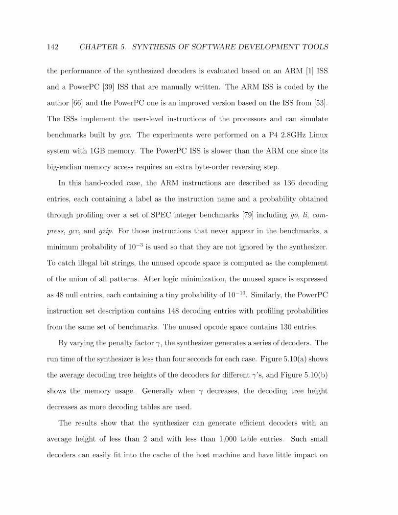
142 CHAPTER 5. SYNTHESIS OF SOFTWARE DEVELOPMENT TOOLS
the performance of the synthesized decoders is evaluated based on an ARM [1] ISS
and a PowerPC [39] ISS that are manually written. The ARM ISS is coded by the
author [66] and the PowerPC one is an improved version based on the ISS from [53].
The ISSs implement the user-level instructions of the processors and can simulate
benchmarks built by gcc. The experiments were performed on a P4 2.8GHz Linux
system with 1GB memory. The PowerPC ISS is slower than the ARM one since its
big-endian memory access requires an extra byte-order reversing step.
In this hand-coded case, the ARM instructions are described as 136 decoding
entries, each containing a label as the instruction name and a probability obtained
through profiling over a set of SPEC integer benchmarks [79] including go, li, com-
press, gcc, and gzip. For those instructions that never appear in the benchmarks, a
minimum probability of 10−3 is used so that they are not ignored by the synthesizer.
To catch illegal bit strings, the unused opcode space is computed as the complement
of the union of all patterns. After logic minimization, the unused space is expressed
as 48 null entries, each containing a tiny probability of 10−10. Similarly, the PowerPC
instruction set description contains 148 decoding entries with profiling probabilities
from the same set of benchmarks. The unused opcode space contains 130 entries.
By varying the penalty factor γ, the synthesizer generates a series of decoders. The
run time of the synthesizer is less than four seconds for each case. Figure 5.10(a) shows
the average decoding tree heights of the decoders for different γ’s, and Figure 5.10(b)
shows the memory usage. Generally when γ decreases, the decoding tree height
decreases as more decoding tables are used.
The results show that the synthesizer can generate efficient decoders with an
average height of less than 2 and with less than 1,000 table entries. Such small
decoders can easily fit into the cache of the host machine and have little impact on
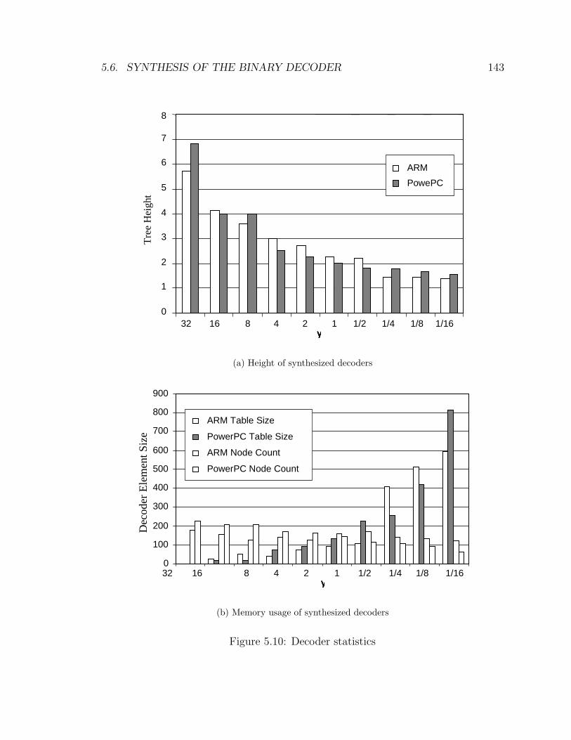
5.6. SYNTHESIS OF THE BINARY DECODER 143
0
1
2
3
4
5
6
7
8
32 16 8 4 2 1 1/2 1/4 1/8 1/16 γγγγ
ARM
PowePC
Tre
e H
eigh
t
(a) Height of synthesized decoders
0
100
200
300
400
500
600
700
800
900
ARM Table Size
PowerPC Table Size
ARM Node Count
PowerPC Node Count
32 16 8 4 2 1 1/2 1/4 1/8 1/16 γγγγ
Dec
oder
Ele
men
t Siz
e
(b) Memory usage of synthesized decoders
Figure 5.10: Decoder statistics
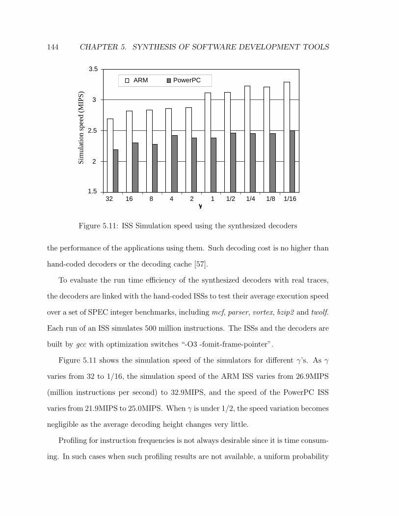
144 CHAPTER 5. SYNTHESIS OF SOFTWARE DEVELOPMENT TOOLS
Si
mul
atio
n sp
eed
(MIP
S)
32 16 1.5
2
2.5
3
3.5
ARM PowerPC
8 4 2 1 1/2 1/4 1/8 1/16 γγγγ
Figure 5.11: ISS Simulation speed using the synthesized decoders
the performance of the applications using them. Such decoding cost is no higher than
hand-coded decoders or the decoding cache [57].
To evaluate the run time efficiency of the synthesized decoders with real traces,
the decoders are linked with the hand-coded ISSs to test their average execution speed
over a set of SPEC integer benchmarks, including mcf, parser, vortex, bzip2 and twolf.
Each run of an ISS simulates 500 million instructions. The ISSs and the decoders are
built by gcc with optimization switches “-O3 -fomit-frame-pointer”.
Figure 5.11 shows the simulation speed of the simulators for different γ’s. As γ
varies from 32 to 1/16, the simulation speed of the ARM ISS varies from 26.9MIPS
(million instructions per second) to 32.9MIPS, and the speed of the PowerPC ISS
varies from 21.9MIPS to 25.0MIPS. When γ is under 1/2, the speed variation becomes
negligible as the average decoding height changes very little.
Profiling for instruction frequencies is not always desirable since it is time consum-
ing. In such cases when such profiling results are not available, a uniform probability
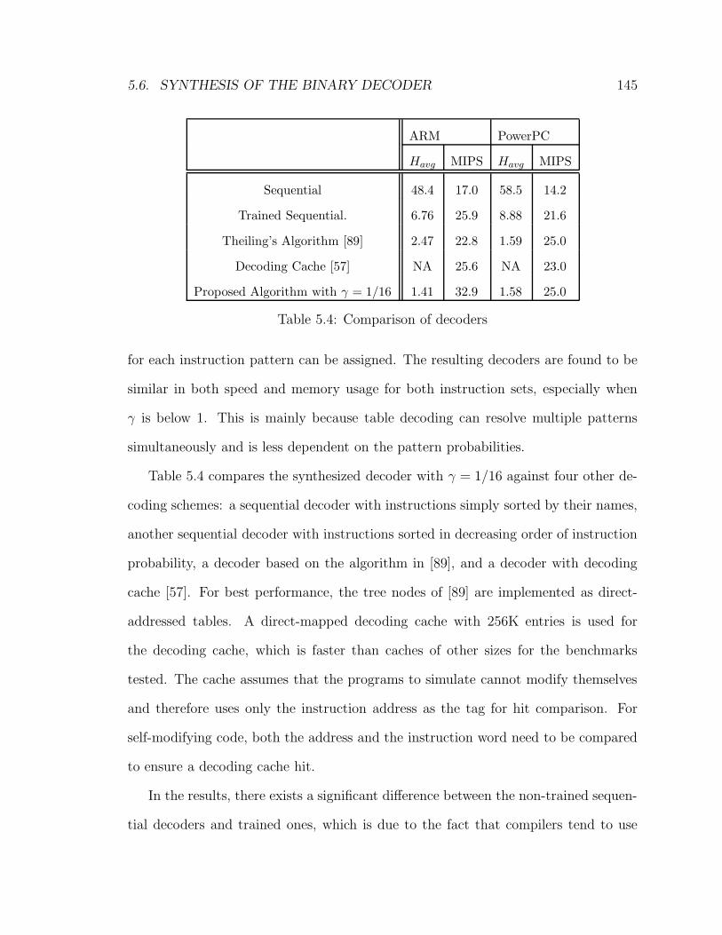
5.6. SYNTHESIS OF THE BINARY DECODER 145
ARM PowerPC
Havg MIPS Havg MIPS
Sequential 48.4 17.0 58.5 14.2
Trained Sequential. 6.76 25.9 8.88 21.6
Theiling’s Algorithm [89] 2.47 22.8 1.59 25.0
Decoding Cache [57] NA 25.6 NA 23.0
Proposed Algorithm with γ = 1/16 1.41 32.9 1.58 25.0
Table 5.4: Comparison of decoders
for each instruction pattern can be assigned. The resulting decoders are found to be
similar in both speed and memory usage for both instruction sets, especially when
γ is below 1. This is mainly because table decoding can resolve multiple patterns
simultaneously and is less dependent on the pattern probabilities.
Table 5.4 compares the synthesized decoder with γ = 1/16 against four other de-
coding schemes: a sequential decoder with instructions simply sorted by their names,
another sequential decoder with instructions sorted in decreasing order of instruction
probability, a decoder based on the algorithm in [89], and a decoder with decoding
cache [57]. For best performance, the tree nodes of [89] are implemented as direct-
addressed tables. A direct-mapped decoding cache with 256K entries is used for
the decoding cache, which is faster than caches of other sizes for the benchmarks
tested. The cache assumes that the programs to simulate cannot modify themselves
and therefore uses only the instruction address as the tag for hit comparison. For
self-modifying code, both the address and the instruction word need to be compared
to ensure a decoding cache hit.
In the results, there exists a significant difference between the non-trained sequen-
tial decoders and trained ones, which is due to the fact that compilers tend to use
146 CHAPTER 5. SYNTHESIS OF SOFTWARE DEVELOPMENT TOOLS
a small set of instructions more frequently than others. In the trained cases, the
decoders try to match with the most frequently used instruction patterns first and
therefore have good performance on the average. However, for benchmarks differing
greatly in instruction frequency from the training set, the result can be much worse.
For instance, the PowerPC decoder trained by integer benchmarks yields an average
decoding height of 29.9 for floating-point benchmarks and a reduced simulation speed
of 17.0MIPS. The algorithm in [89] generates very good decision trees. For the Pow-
erPC instruction set, which is regularly laid out as two levels of opcodes, the resulting
decision tree is almost of the same height as the proposed approach. However, for the
ARM instruction set with complex encoding, its tree is taller. Since the tree nodes of
the algorithm involve table decoding based on non-contiguous bits of the instruction
word, the resulting ARM decoder is slower than the proposed one. Moreover, for both
instruction sets it is possible to add new instruction patterns that cause the algorithm
of [89] to fail. The decoders utilizing decoding caches have moderate performance as
shown in Table 5.4. As a cache lookup involves in the least a table lookup, a valid-bit
test and a tag comparison, it can hardly be more efficient than the short decoding
tree generated by the proposed algorithm. In a more general implementation which
allows self-modifying code simulation, the tag comparison needs to take into account
the instruction word. Very likely the decoding cache will be even slower. In contrast,
no modification is needed to the other decoders for simulating self-modifying code.
The evaluation results here were all based on the particular ISSs mentioned above.
They have a slow down factor of around 100, which means that on average it takes
about 100 native instructions to interpret a target instruction. For faster ISS imple-
mentations, the efficiency benefit of the proposed algorithm will be more significant.
Although its effect in the MADL-based simulator synthesis framework is not as sig-
5.7. SUMMARY 147
nificant, after more aggressive optimization is implemented in the framework, the
benefit will likely become more apparent.
Overall, the decoder synthesis algorithm requires very simple input in the form of
decoding entries, which can be easily extracted from MADL descriptions. Therefore
the synthesizer has been easily integrated into the simulation framework described
in Section 5.2 and Section 5.3. The simulator synthesis framework checks the well-
formed property of the patterns and computes the unused pattern space. It then
assigns a uniform probability to each used pattern and a tiny probability to each
unused pattern. The resulting decoding entries are used to as the input to the decoder
synthesizer.
5.7 Summary
This chapter described several tools that are implemented based on MADL. They
include a simulator synthesis framework for CASs and ISSs, a disassembler synthe-
sizer, a tool that extracts reservation tables, and a binary decoder synthesizer. The
design of MADL and most of the software tools has been published in a conference
paper [70]. The binary decoder synthesizer has been presented at the 40th Design
Automation Conference [68].
The simulator synthesis framework simplifies the implementation of the hardware
level by using a clock-driven kernel and a communication mechanism based on inter-
face function calls. It also optimizes the steering of the OSM at the decoding points.
With these techniques, the framework is capable of synthesizing highly efficient CASs.
In the StrongARM case, the synthesized CAS outperforms the hand-optimized CASs
by a great margin.
148 CHAPTER 5. SYNTHESIS OF SOFTWARE DEVELOPMENT TOOLS
By transforming the state diagram into a control flow graph, the simulator syn-
thesis framework can generate semantics evaluation procedures for operations. After
further simplification of the hardware level by removing timing or concurrency related
control policies and some components such as caches, ISSs can be generated from these
procedures. Because the same MADL descriptions for CASs can be reused for ISS
synthesis, the modeling productivity gain is significant.
As a part of the simulator synthesis framework, a new binary decoder synthesis
algorithm was designed and implemented. The binary decoding synthesis problem
was formulated as a decoding tree construction process. With carefully chosen de-
coding functions and cost model, effective heuristics was developed to guide the tree
construction process. The resulting synthesizer can generate fast binary decoders
with guaranteed correctness.
The assembly chunks specified in the MADL description can be stitched together
according to the expansions of the AND-OR graph. The resulting assembly templates
are used to generate disassemblers.
To demonstrate the analyzability property of MADL, a reservation table extractor
was implemented. With the help of annotations, the tool can obtain information such
as the execution paths and the resource usages of an operation. Such information can
be used by list schedulers in HLL compilers.
In summary, the chapter demonstrated that MADL inherits the nice properties of
the OSM model. It is flexible as it can be used to specify various styles of processor
design. It is efficient as it supports the generation of very fast simulators. It is ana-
lyzable in that it supports the extraction of operation properties. And it is compact
as the MADL description is short and the same description can be used in generating
different software tools.
Chapter 6
Conclusions
As the design of integrated circuits starts to enter the nanometer design era [41], the
sharply rising design and manufacturing costs are prompting more system designers
to adopt software-based alternatives to the traditional hardwired application-specific
integrated circuits (ASICs). These software-based approaches utilize processors of
various kinds. Among them, application-specific instruction set processors (ASIPs)
are of particular interest to designers in that their domain-specific features offer high
power and performance efficiencies. To automate the development of ASIPs, software
tools such as simulators and high-level language compilers are needed. In the early
development stages of an ASIP, these tools help to evaluate design decisions and
guide the design space optimization process. To explore a reasonably large space for
a satisfactory final design point, it is necessary to automate the generation of these
software tools from a high-level processor specification.
As an important but challenging problem, automated generation of the software
tools has been the research focus of many research groups in both industry and
academia. The key perspective that leads to an insightful understanding of the exist-
149
150 CHAPTER 6. CONCLUSIONS
ing approaches is the architecture model – the computation model used to represent
the concurrency in the processor. Due to the different needs of researchers, architec-
ture models with various degrees of emphasis on either the microarchitecture or the
instruction set architecture have been used. The representative ones include the dis-
crete event model, the clock-driven model, the heterogeneous synchronous/reactive
model, the Gantt-Chart model, and architecture templates. They reflect different
trade-offs between abstraction level and flexibility. To evaluate their suitability as
the basis for the synthesis of software tools, the following four properties need to be
considered.
Compactness – The effort that it takes to specify a processor based on the model.
Flexibility – The range of architectures supported by the model.
Efficiency – The potential execution speed of the model.
Analyzability – The possibility to extract model properties for analysis.
These properties are often conflicting with each other. Therefore, it is impossible
to create an architecture model that is excellent in all four aspects without compro-
mise. A practical approach is to find one that is well balanced among the properties
for the particular needs of the designer. The focus of the dissertation is to find such
a model for embedded processor design at the system level.
6.1 Contributions
The main contribution of the dissertation is the proposal of the operation state ma-
chine (OSM) model. The model views a processor from two angles simultaneously. In
6.1. CONTRIBUTIONS 151
the operation view, operations are modeled as extended finite state machines (EFSM).
The states of an EFSM represent the execution statuses of the operation and the edges
represent the execution paths and conditions. These EFSMs form the operation level
of the OSM model. In the hardware view, the microarchitecture components interact
with each other in an event-driven fashion. These components constitute the hard-
ware level of the model. Using the abstract notion of token for all data and control
resources, the OSM model connects the two levels with a simple token-based commu-
nication interface. In essence, the OSM model separately captures the concurrency
among the operations, the concurrency among the microarchitectural components,
and the interaction between the operations and the microarchitectural components.
Due to the high-level abstractions including the EFSMs and the tokens, the hard-
ware components in the OSM model are greatly simplified compared with those in
structural modeling approaches. Therefore, it is relatively easy to specify an OSM-
based processor model. Also, due to the use of abstractions, the resulting processor
model has better execution speed than pure DE-based structural models. Moreover,
as the token transactions between the operations and the hardware components are
explicit in the model, it is easy to analyze the resource consumptions and potentially
other properties of the operations. Despite the use of the high-level abstractions, the
OSM model is shown to be flexible in modeling a wide range of architecture features
of modern processors. Overall, the OSM model is very well balanced among the
aforementioned four properties and is thus suitable to be used for the synthesis of
software tools.
In order to allow for the convenient specification of OSM-based processor models,
the MESCAL Architecture Description Language (MADL) is developed. The lan-
guage features a description structure with two closely related layers, including the
152 CHAPTER 6. CONCLUSIONS
core layer that supports concise description of the EFSMs of the OSM model, and the
annotation layer that supplies tool-dependent hints or extra information to various
software tools. The two-layer approach insulates core descriptions from frequent ex-
tensions of the software tools and consequently frequent changes of the tool-dependent
information, lengthening the life time of the core layer.
The syntax design of the core layer utilizes the AND-OR graph technique to
minimize redundancy in descriptions. To apply the AND-OR graph technique, the
OSM model is adapted to its dynamic version, in which the operation properties are
dynamically bound to the state diagram during execution. The dynamic OSM model
integrates well with the AND-OR graph technique and forms the foundation of the
core layer. A simple transformation technique can be used to translate a dynamic
model specified by MADL back to the original OSM model.
The novel two-layer structure of MADL and the integration of the OSM model
with the AND-OR graph technique constitute the second contribution of the dis-
sertation. The former is unique in that it is the first known description scheme that
explicitly separates tool-dependent information from key architecture properties. The
latter enables easy specification of the OSM model and makes its full use practical.
To demonstrate the effectiveness of the OSM model and MADL, the dissertation
describes an MADL-based simulator synthesis framework that is capable of generat-
ing cycle-accurate simulators (CASs) and instruction set simulators (ISSs). For fast
simulation speed of the synthesized simulators, a couple of simplification techniques
are used. These include using a clock-driven kernel for the hardware level of the OSM
model and using a function-call-based communication mechanism for the hardware
components. The resulting CASs prove to have leading performance among the same
class of simulators. As a by-product of the simulation framework, a disassembler
6.2. FUTURE WORK 153
synthesizer is implemented. The synthesized disassemblers can be used to dump ex-
ecution traces of the simulators for debugging purposes. The development of these
tools provide supportive evidence that the OSM model and MADL are suitable to be
used as the foundation for the synthesis of software tools.
To optimize the decoding behavior of the state machines, an efficient binary de-
coder synthesis algorithm is proposed. Given a set of operation encoding patterns
extracted from an MADL description, the decoder synthesizer can generate very ef-
ficient decoding trees to be used by the CAS, the ISS, and the disassembler. For
speed critical software tools such as hand-crafted ISSs, the speed advantage of the
synthesized decoders is significant compared to competing algorithms.
Last but not least, as a demonstration of the analyzability property of the OSM
model, the dissertation described a tool that extracts reservation tables from MADL
descriptions. With the help of a small amount of annotation, the tool can obtain
information such as the execution paths and the resource usages of an operation.
The information can be used by list schedulers in HLL compilers.
6.2 Future Work
Despite its over-two-decade history and the large number of dedicated research groups,
the field of design automation of ASIPs and associated software tools is far from being
mature. Novel models and algorithms, as well as persistent engineering efforts, are
indispensable to push the envelope. This work is one such effort that results in the
conception of the promising OSM model.
Research involving the OSM model and MADL is not yet complete. A few direc-
tions are worth exploring. First, as MADL currently supports only the description
154 CHAPTER 6. CONCLUSIONS
of the operation level of the OSM model, it is a natural thought to extend MADL so
as to cover the hardware level. Such extension requires the formal modeling of the
token management policies in the hardware level, which is a non-trivial but highly
rewarding task. A clean extension of MADL into the hardware level may open doors
to research directions such as formal verification of a processor specification and high-
level synthesis of processor hardware from MADL.
Second, the software tools supported by MADL do not yet form a complete tool-
chain that allows design space exploration for ASIP design. The major missing com-
ponent is the compiler. Admittedly, developing a user-retargetable compiler for a
wide range of processors is an overwhelming challenge given the current status of
retargetable compilation techniques. A practical approach is to develop a library of
compiler components that can be retargeted by MADL. With the library, designers
can quickly assemble a retargetable compiler for a new family of processors under
consideration.
Third, to allow MADL-based processor models to integrate with system level sim-
ulators, the hardware level of the OSM model may be considered for implementation
in SystemC, a standard system-level modeling language. Although the simulation
speed is likely to drop a bit since SystemC utilizes the discrete-event kernel, the
utility of the models should increase as they can be readily integrated into other
SystemC-based modeling environments. A similarly interesting idea is to implement
the hardware level of the OSM model with the heterogeneous synchronous/reactive
simulation kernel of LSE [92].
Overall, OSM-based modeling is a promising approach for ASIP design. With
continuous future efforts along this direction, it is possible that the OSM model
becomes the foundation of a suite of commercial software tools.
Appendix A
The MESCAL Architecture
Description Language V1.0
Reference Manual
A.1 Introduction
The MESCAL Architecture Description Language (MADL) specifies the operation
state machine model (OSM) for microprocessor modeling purposes. It supplies pro-
cessor information to software tools including the instruction set simulator, the mi-
croarchitecture simulator, the assembler, the disassembler, and various compiler op-
timizers.
MADL is composed of two parts: the core language and the annotation lan-
guage. The core language describes the operation state machines of the OSM model,
which have concrete executable semantics. The annotation language describes tool-
dependent information. For any tool that utilizes MADL, an annotation description
155
156 APPENDIX A. MADL V1.0 REFERENCE MANUAL
scheme can be created based on the generic annotation syntax. The annotation de-
scription supplements with information such as hints for the tool to analyze the core
description. This document mainly describes the syntax of the core language. The
generic syntax of the annotation language is described in Section A.12.
Note that currently the hardware layer of the OSM model is not part of MADL.
The execution model of the hardware units, including the token managers, are im-
plemented in the general-purpose programming language C++, which is the target
language into which MADL descriptions are to be translated for execution. MADL
1.0 only declares the names and the types of the token managers. Description of the
hardware layer is expected to be included in future versions of MADL.
MADL utilizes a hierarchical description structure called the AND-OR graph to
minimize redundancy in descriptions. To integrate the OSM model with the AND-
OR graph, MADL uses a dynamic version of the OSM model. The feature of the
dynamic model is that the actions and computations are dynamically bound to the
edges of the state diagram. A well-defined dynamic model can be transformed back
to a static model. Besides token managers, the entities in the dynamic OSM model
include the skeleton and the syntax operation. A skeleton refers to the state diagram
and the internal state variables associated with it. A syntax operation refers to a set
of actions and computations, as well as assembly syntax and binary encoding. The
syntax operations form an AND-OR graph. A skeleton and all syntax operations
in an expansion of the AND-OR graph constitute the model of one operation in
the instruction set. These syntax operations are dynamically bound to the skeleton
during execution.
An MADL file may contain any number of the following sections,
1. Define Section — declaration of global variables/functions.
A.1. INTRODUCTION 157
2. Manager Section — declaration of token managers.
3. Machine Section — definition of a skeleton.
4. Function Section — definition of a function.
5. Operation Section — definition of a syntax operation.
Besides, an MADL file may also contain the following commands.
1. Import command — including other MADL files to the same description. Its
syntax is shown below.
import_command ::= "IMPORT" ’"’identifier ’"’ ’;’
2. Using command — associating skeleton with syntax operations. A using com-
mand states that all operation sections from the command until the next using
command or the end of the file, whichever comes first, are based on the skeleton
with the given name. Its syntax is shown below.
using_command ::= "USING" identifier ’;’
Except for the using command, all other sections in MADL are order-independent.
For instance, a function section may appear anywhere in an MADL description, either
before or after its caller(s). Comments can be placed anywhere in a MADL descrip-
tion. Two types of comments are allowed: single-line comment and block comment.
A single-line comment starts with a ’#’ and lasts until the end of the line. A block
comment starts with a “##” and lasts until another “##”.
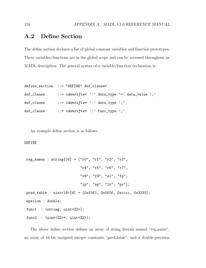
158 APPENDIX A. MADL V1.0 REFERENCE MANUAL
A.2 Define Section
The define section declares a list of global constant variables and function prototypes.
These variables/functions are in the global scope and can be accessed throughout an
MADL description. The general syntax of a variable/function declaration is:
define_section ::= "DEFINE" def_clause+
def_clause ::= identifier ’:’ data_type ’=’ data_value ’;’
def_clause ::= identifier ’:’ data_type ’;’
def_clause ::= identifier ’:’ func_type ’;’
An example define section is as follows.
DEFINE
reg_names : string[16] = {"r0", "r1", "r2", "r3",
"r4", "r5", "r6", "r7",
"r8", "r9", "sl", "fp",
"ip", "sp", "lr", "pc"};
pred_table : uint<16>[4] = {0xf0f0, 0x0f0f, 0xcccc, 0x3333};
epsilon : double;
func1 : (string, uint<32>);
func2 : (uint<32>*, uint<32>);
The above define section defines an array of string literals named “reg name”,
an array of 16-bit unsigned integer constants “pred table”, and a double-precision
A.3. MANAGER SECTION 159
constant “epsilon” whose value is not given. Additionally, it defines two functions
“func1” and “func2”. Function arguments in MADL are passed by reference. Writable
arguments are denoted by a “*” after the argument type, e.g. the first argument of
“func2”. The value of a writable argument may be changed by the function. The
variables without values and the functions should be defined in external C++ files for
simulation purposes. These C++ files should be linked with MADL generated C++
files in simulators.
For syntax of data and function types, refer to Section A.8 of the document. The
restriction is that no void or tuple data types can be used in define sections.
A.3 Manager Section
In the OSM model, data or structural resources are modeled as tokens and are man-
aged by token managers. A state machine transacts tokens with the token managers
during its execution. In order to get a token, it will typically present to the token
manager an index as a token identifier. The manager will then return a token if it is
available. The state machine may also read value from and write value to the tokens
that it can access. A list of possible token transactions (also called actions) and their
description syntax is given in Section A.11.
A manager section may contain a CLASS subsection and an INSTANCE subsec-
tion. The former declares token manager class names and their types, while the latter
declares token manager instances. A type here is a tuple of the token index type and
the token value type. All data types except array can be used as index or value type.
The syntax of the section is shown below.
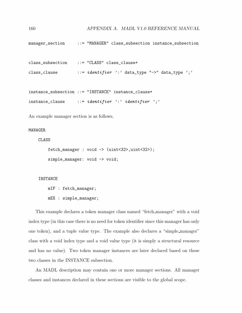
160 APPENDIX A. MADL V1.0 REFERENCE MANUAL
manager_section ::= "MANAGER" class_subsection instance_subsection
class_subsection ::= "CLASS" class_clause+
class_clause ::= identifier ’:’ data_type "->" data_type ’;’
instance_subsection ::= "INSTANCE" instance_clause+
instance_clause ::= identifier ’:’ identifier ’;’
An example manager section is as follows.
MANAGER
CLASS
fetch_manager : void -> (uint<32>,uint<32>);
simple_manager: void -> void;
INSTANCE
mIF : fetch_manager;
mEX : simple_manager;
This example declares a token manager class named “fetch manager” with a void
index type (in this case there is no need for token identifier since this manager has only
one token), and a tuple value type. The example also declares a “simple manager”
class with a void index type and a void value type (it is simply a structural resource
and has no value). Two token manager instances are later declared based on these
two classes in the INSTANCE subsection.
An MADL description may contain one or more manager sections. All manager
classes and instances declared in these sections are visible to the global scope.
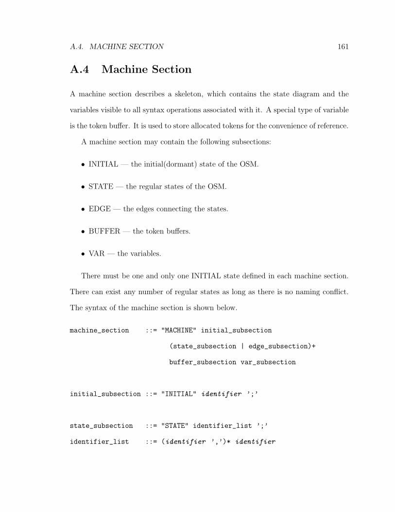
A.4. MACHINE SECTION 161
A.4 Machine Section
A machine section describes a skeleton, which contains the state diagram and the
variables visible to all syntax operations associated with it. A special type of variable
is the token buffer. It is used to store allocated tokens for the convenience of reference.
A machine section may contain the following subsections:
• INITIAL — the initial(dormant) state of the OSM.
• STATE — the regular states of the OSM.
• EDGE — the edges connecting the states.
• BUFFER — the token buffers.
• VAR — the variables.
There must be one and only one INITIAL state defined in each machine section.
There can exist any number of regular states as long as there is no naming conflict.
The syntax of the machine section is shown below.
machine_section ::= "MACHINE" initial_subsection
(state_subsection | edge_subsection)+
buffer_subsection var_subsection
initial_subsection ::= "INITIAL" identifier ’;’
state_subsection ::= "STATE" identifier_list ’;’
identifier_list ::= (identifier ’,’)* identifier
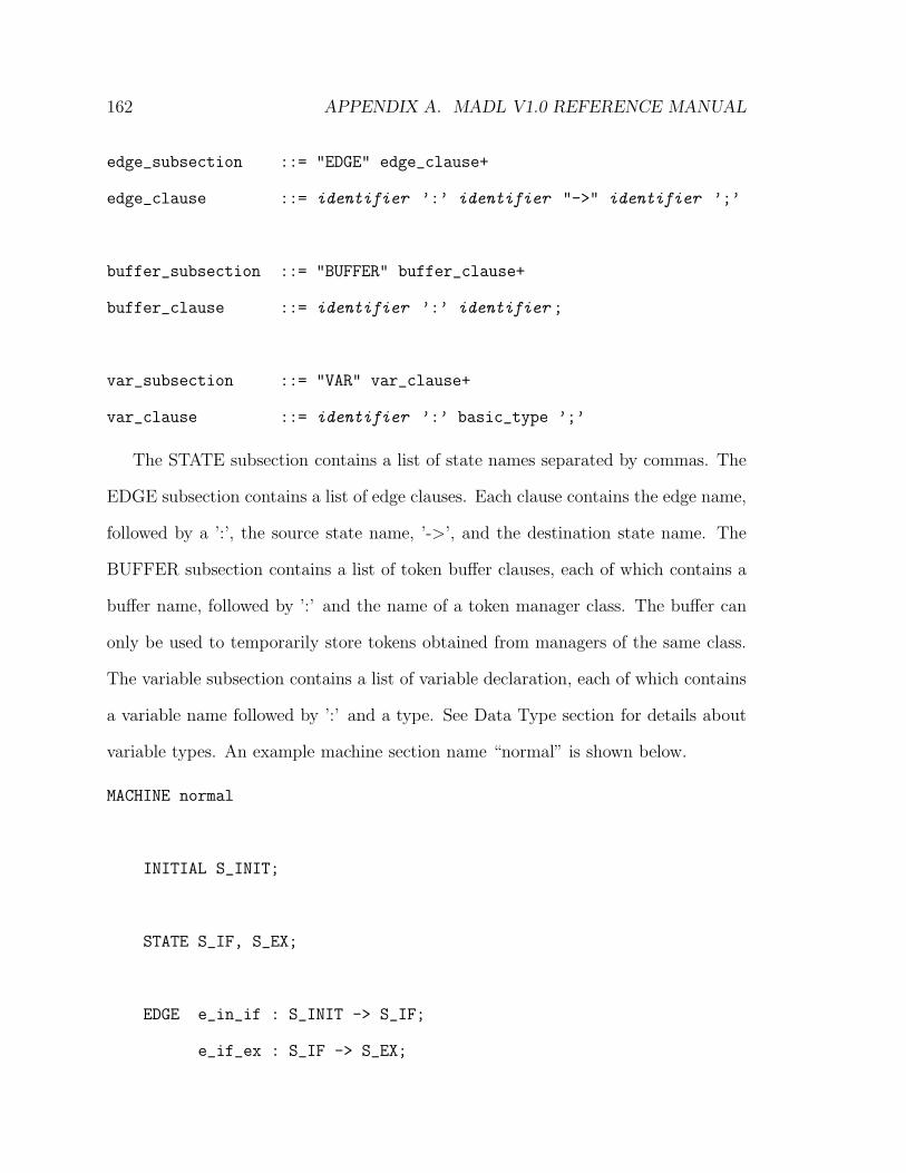
162 APPENDIX A. MADL V1.0 REFERENCE MANUAL
edge_subsection ::= "EDGE" edge_clause+
edge_clause ::= identifier ’:’ identifier "->" identifier ’;’
buffer_subsection ::= "BUFFER" buffer_clause+
buffer_clause ::= identifier ’:’ identifier ;
var_subsection ::= "VAR" var_clause+
var_clause ::= identifier ’:’ basic_type ’;’
The STATE subsection contains a list of state names separated by commas. The
EDGE subsection contains a list of edge clauses. Each clause contains the edge name,
followed by a ’:’, the source state name, ’->’, and the destination state name. The
BUFFER subsection contains a list of token buffer clauses, each of which contains a
buffer name, followed by ’:’ and the name of a token manager class. The buffer can
only be used to temporarily store tokens obtained from managers of the same class.
The variable subsection contains a list of variable declaration, each of which contains
a variable name followed by ’:’ and a type. See Data Type section for details about
variable types. An example machine section name “normal” is shown below.
MACHINE normal
INITIAL S_INIT;
STATE S_IF, S_EX;
EDGE e_in_if : S_INIT -> S_IF;
e_if_ex : S_IF -> S_EX;
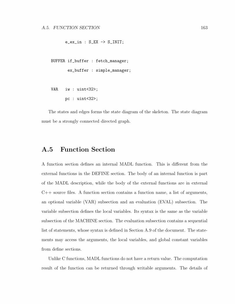
A.5. FUNCTION SECTION 163
e_ex_in : S_EX -> S_INIT;
BUFFER if_buffer : fetch_manager;
ex_buffer : simple_manager;
VAR iw : uint<32>;
pc : uint<32>;
The states and edges forms the state diagram of the skeleton. The state diagram
must be a strongly connected directed graph.
A.5 Function Section
A function section defines an internal MADL function. This is different from the
external functions in the DEFINE section. The body of an internal function is part
of the MADL description, while the body of the external functions are in external
C++ source files. A function section contains a function name, a list of arguments,
an optional variable (VAR) subsection and an evaluation (EVAL) subsection. The
variable subsection defines the local variables. Its syntax is the same as the variable
subsection of the MACHINE section. The evaluation subsection contains a sequential
list of statements, whose syntax is defined in Section A.9 of the document. The state-
ments may access the arguments, the local variables, and global constant variables
from define sections.
Unlike C functions, MADL functions do not have a return value. The computation
result of the function can be returned through writable arguments. The details of
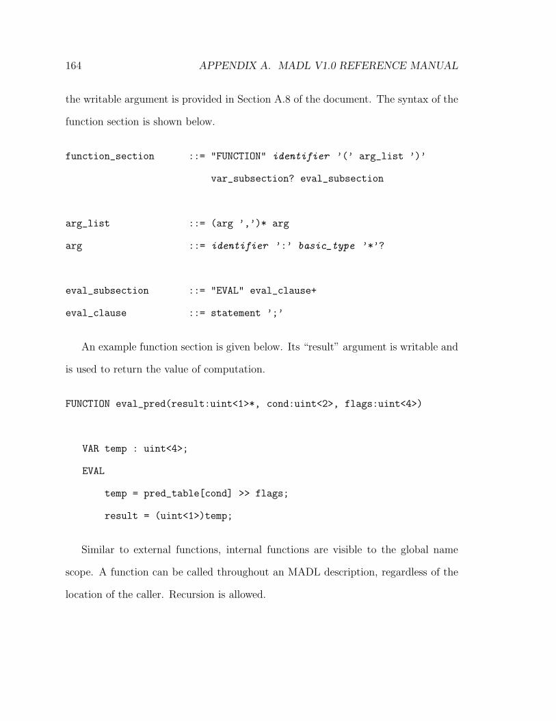
164 APPENDIX A. MADL V1.0 REFERENCE MANUAL
the writable argument is provided in Section A.8 of the document. The syntax of the
function section is shown below.
function_section ::= "FUNCTION" identifier ’(’ arg_list ’)’
var_subsection? eval_subsection
arg_list ::= (arg ’,’)* arg
arg ::= identifier ’:’ basic_type ’*’?
eval_subsection ::= "EVAL" eval_clause+
eval_clause ::= statement ’;’
An example function section is given below. Its “result” argument is writable and
is used to return the value of computation.
FUNCTION eval_pred(result:uint<1>*, cond:uint<2>, flags:uint<4>)
VAR temp : uint<4>;
EVAL
temp = pred_table[cond] >> flags;
result = (uint<1>)temp;
Similar to external functions, internal functions are visible to the global name
scope. A function can be called throughout an MADL description, regardless of the
location of the caller. Recursion is allowed.
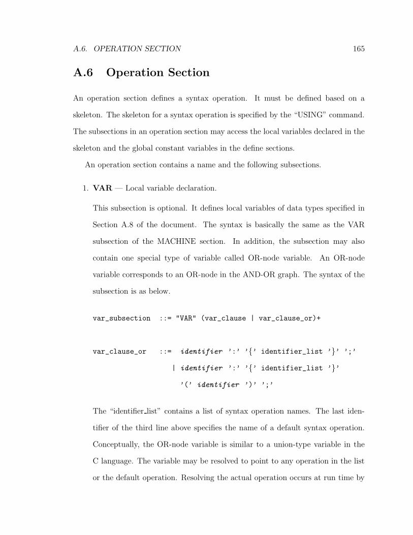
A.6. OPERATION SECTION 165
A.6 Operation Section
An operation section defines a syntax operation. It must be defined based on a
skeleton. The skeleton for a syntax operation is specified by the “USING” command.
The subsections in an operation section may access the local variables declared in the
skeleton and the global constant variables in the define sections.
An operation section contains a name and the following subsections.
1. VAR — Local variable declaration.
This subsection is optional. It defines local variables of data types specified in
Section A.8 of the document. The syntax is basically the same as the VAR
subsection of the MACHINE section. In addition, the subsection may also
contain one special type of variable called OR-node variable. An OR-node
variable corresponds to an OR-node in the AND-OR graph. The syntax of the
subsection is as below.
var_subsection ::= "VAR" (var_clause | var_clause_or)+
var_clause_or ::= identifier ’:’ ’{’ identifier_list ’}’ ’;’
| identifier ’:’ ’{’ identifier_list ’}’
’(’ identifier ’)’ ’;’
The “identifier list” contains a list of syntax operation names. The last iden-
tifier of the third line above specifies the name of a default syntax operation.
Conceptually, the OR-node variable is similar to a union-type variable in the
C language. The variable may be resolved to point to any operation in the list
or the default operation. Resolving the actual operation occurs at run time by
166 APPENDIX A. MADL V1.0 REFERENCE MANUAL
decoding: the encodings (specified by CODING subsection) of the operations
in the identifier list will be pattern-matched against a given binary value and
the matching one will be chosen. If no one matches and a default operation is
given, the default operation will be chosen. If no default operation is provided, a
run-time error will be reported. If more than one operation matches, the closest
match will be chosen. A valid OR-node variable requires that all operations in
the name list have the same encoding width. Such an encoding width is viewed
as the encoding width of the OR-node variable. Decoding is triggered by the
decode statement or the activate statement. See details of the statements in
description of the EVAL subsection.
A predefined variable “coding” can be used throughout the operation section if
it contains a CODING subsection. The variable has an unsigned integer type
of the same width as that of the encoding of the operation (the sum of the data
widths of all elements in the CODING).
2. SYNTAX — Assembly syntax of the operation.
The subsection contains a list of syntax elements separated by blank spaces or
carets. When two elements are separated by a blank space, there will be a space
in between in the assembly output. Otherwise, the two will be joined together.
A syntax element can be any of the following:
• String literal, e.g. “ldw”.
• A variable, e.g. v1. The variable can be a local variable or one declared in
the machine section or in the define section. Modifiers can be used here
to specify the output format when converting arithmetic data values to
string.
A.6. OPERATION SECTION 167
• Table lookup, e.g. array[v1]. The table should be defined in the define
section. Modifiers can also be used here.
The syntax of this subsection is shown below
syntax_subsection ::= "SYNTAX" (syntax_clause ’^’?)*
syntax_clause ’;’
syntax_clause ::= ’"’ string ’"’
| identifier modifier?
| identifier ’[’ identifier ’]’ modifier?
3. CODING — Binary encoding of the operation.
The subsection contains a list of coding elements separated by blank spaces. A
coding element can be any of the following.
• Boolean literal — string of 0, 1 and -, such as 00--11-.
• A variable, e.g. v1.
• OR-ed boolean literals, e.g. (0011 | 1100).
The syntax of this subsection is shown below
coding_subsection ::= "CODING" coding_clause+ ’;’
coding_clause_or ::= boolean_literal
| identifier
| ’(’ (bool_literal ’|’)+ bool_literal ’)’
bool_literal ::= (’0’|’1’|’-’)+
168 APPENDIX A. MADL V1.0 REFERENCE MANUAL
4. EVAL — Initialization actions.
This subsection contains the actions to be performed at the moment when the
syntax operation is bound to the skeleton at run-time. Similar to the EVAL
subsection in function section, this subsection contains a sequential list of state-
ments. In addition to the statements defined in Section A.9 of the document,
two other types of statements are supported here.
(a) Decode Statement.
The syntax of a decode statement is
statement_decode ::= ’+’ identifier = identifier
| ’+’ identifier
(b) Activate Statement.
statement_activate ::= ’@’ identifier = identifier
| ’@’ identifier
For both statements, the first identifier must be an OR-node variable. The
optional second identifier must have identical encoding width to that of the
OR-node variable. The second identifier specifies the actual binary value that
is used to decode the OR-node variable. It should be omitted if the OR-node
variable appears in the coding section of the operation. In this case MADL will
extract the corresponding binary field from coding and use it to decode.
Both statements will trigger a decoding procedure to resolve the actual syntax
operation. After decoding, the decode statement will evaluate the EVAL sub-
section of the resolved operation (the closest match in the list of the OR-node
variable) and annotate its actions and computations (defined in the TRANS
A.6. OPERATION SECTION 169
subsection) on the current skeleton. In contrast, the activate statement will
spawn another state machine and then let the resolved operation evaluate its
EVAL subsection and annotate its actions and computations onto the spawned
skeleton.
5. TRANS — Actions and computations.
The TRANS subsection describes the actions and computation statements as-
sociated with the OSM edges. The syntax of the subsection is shown below.
trans_subsection ::= "TRANS" trans_clause+
trans_clause ::= identifier ’:’ ’{’ action_list ’}’
statement_list ’;’
| identifier ’:’ statement_list ’;’
action_list ::= nil
| (action ’,’)* action+
statement_list ::= (statement ’;’)*
Both the “action list” and the “statement list” are optional. If both are omit-
ted (and no other syntax operation annotates the edge), it means that state
transfer can occur along this edge unconditionally and without any side-effects.
Section A.11 provides details regarding the actions. The statement list syntax
is the same as that of the EVAL subsection.
The “trans clause” associates the actions and the statements to the edge. It
is likely that multiple syntax operations annotate their actions and statements
onto the same edge. The actual firing order of these actions and statements is
described in Section A.7. If an edge is not annotated by any syntax operation
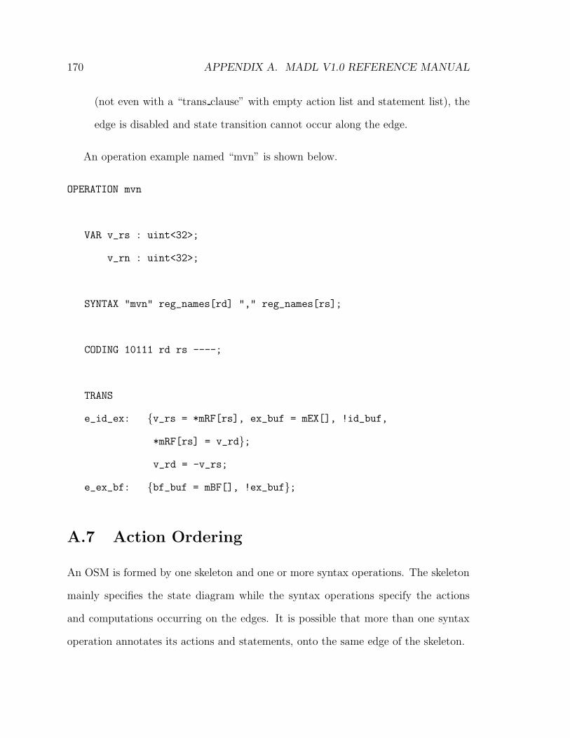
170 APPENDIX A. MADL V1.0 REFERENCE MANUAL
(not even with a “trans clause” with empty action list and statement list), the
edge is disabled and state transition cannot occur along the edge.
An operation example named “mvn” is shown below.
OPERATION mvn
VAR v_rs : uint<32>;
v_rn : uint<32>;
SYNTAX "mvn" reg_names[rd] "," reg_names[rs];
CODING 10111 rd rs ----;
TRANS
e_id_ex: {v_rs = *mRF[rs], ex_buf = mEX[], !id_buf,
*mRF[rs] = v_rd};
v_rd = -v_rs;
e_ex_bf: {bf_buf = mBF[], !ex_buf};
A.7 Action Ordering
An OSM is formed by one skeleton and one or more syntax operations. The skeleton
mainly specifies the state diagram while the syntax operations specify the actions
and computations occurring on the edges. It is possible that more than one syntax
operation annotates its actions and statements, onto the same edge of the skeleton.
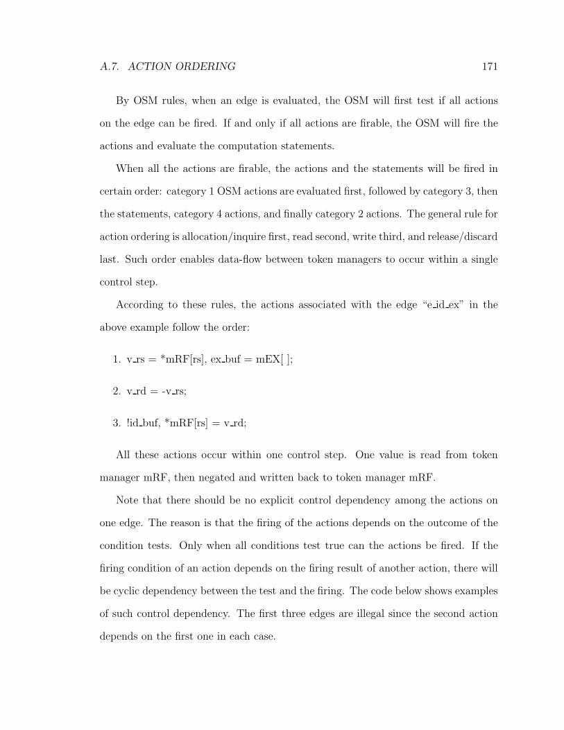
A.7. ACTION ORDERING 171
By OSM rules, when an edge is evaluated, the OSM will first test if all actions
on the edge can be fired. If and only if all actions are firable, the OSM will fire the
actions and evaluate the computation statements.
When all the actions are firable, the actions and the statements will be fired in
certain order: category 1 OSM actions are evaluated first, followed by category 3, then
the statements, category 4 actions, and finally category 2 actions. The general rule for
action ordering is allocation/inquire first, read second, write third, and release/discard
last. Such order enables data-flow between token managers to occur within a single
control step.
According to these rules, the actions associated with the edge “e id ex” in the
above example follow the order:
1. v rs = *mRF[rs], ex buf = mEX[ ];
2. v rd = -v rs;
3. !id buf, *mRF[rs] = v rd;
All these actions occur within one control step. One value is read from token
manager mRF, then negated and written back to token manager mRF.
Note that there should be no explicit control dependency among the actions on
one edge. The reason is that the firing of the actions depends on the outcome of the
condition tests. Only when all conditions test true can the actions be fired. If the
firing condition of an action depends on the firing result of another action, there will
be cyclic dependency between the test and the firing. The code below shows examples
of such control dependency. The first three edges are illegal since the second action
depends on the first one in each case.
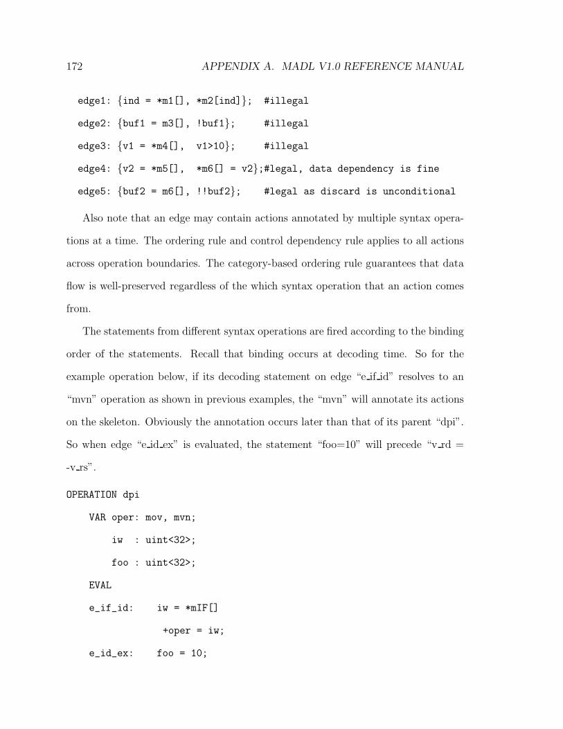
172 APPENDIX A. MADL V1.0 REFERENCE MANUAL
edge1: {ind = *m1[], *m2[ind]}; #illegal
edge2: {buf1 = m3[], !buf1}; #illegal
edge3: {v1 = *m4[], v1>10}; #illegal
edge4: {v2 = *m5[], *m6[] = v2};#legal, data dependency is fine
edge5: {buf2 = m6[], !!buf2}; #legal as discard is unconditional
Also note that an edge may contain actions annotated by multiple syntax opera-
tions at a time. The ordering rule and control dependency rule applies to all actions
across operation boundaries. The category-based ordering rule guarantees that data
flow is well-preserved regardless of the which syntax operation that an action comes
from.
The statements from different syntax operations are fired according to the binding
order of the statements. Recall that binding occurs at decoding time. So for the
example operation below, if its decoding statement on edge “e if id” resolves to an
“mvn” operation as shown in previous examples, the “mvn” will annotate its actions
on the skeleton. Obviously the annotation occurs later than that of its parent “dpi”.
So when edge “e id ex” is evaluated, the statement “foo=10” will precede “v rd =
-v rs”.
OPERATION dpi
VAR oper: mov, mvn;
iw : uint<32>;
foo : uint<32>;
EVAL
e_if_id: iw = *mIF[]
+oper = iw;
e_id_ex: foo = 10;
A.8. DATA TYPES 173
A.8 Data Types
MADL supports the following basic types:
• void
• int<n>— n is the bit width
• uint<n>— n is the bit width
• float— IEEE-754 single precision
• double— IEEE-754 double precision
• string
MADL supports the following complex types:
• array— type[n].
One dimensional array for int, uint, float, double, and string types are sup-
ported. Array type can only be used in global constant variable declaration in
define sections.
• n-tuple— (type1, type2, ...).
A tuple element can be any of the basic types except void. Tuple type can be
used in manager sections as index type or value type. Functions also have tuple
types, either in the function sections where they are defined, or in the define
sections where they are declared as external functions. An element of a function
tuple type can be followed by a ’*’, indicating that this is a writable argument,
viz., the argument is a reference (same as in C++) and may be modified by the
function body. Elements without ’*’s are read-only arguments, similar to const
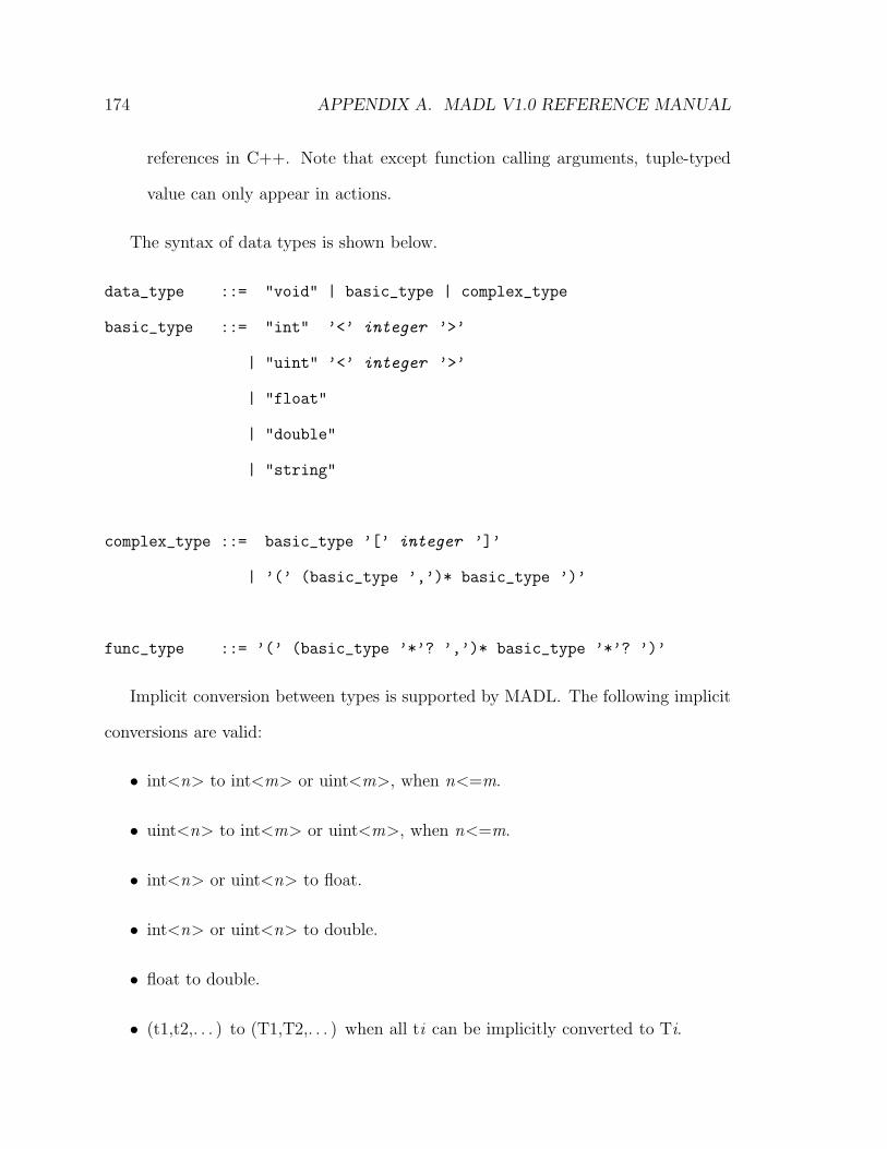
174 APPENDIX A. MADL V1.0 REFERENCE MANUAL
references in C++. Note that except function calling arguments, tuple-typed
value can only appear in actions.
The syntax of data types is shown below.
data_type ::= "void" | basic_type | complex_type
basic_type ::= "int" ’<’ integer ’>’
| "uint" ’<’ integer ’>’
| "float"
| "double"
| "string"
complex_type ::= basic_type ’[’ integer ’]’
| ’(’ (basic_type ’,’)* basic_type ’)’
func_type ::= ’(’ (basic_type ’*’? ’,’)* basic_type ’*’? ’)’
Implicit conversion between types is supported by MADL. The following implicit
conversions are valid:
• int<n> to int<m> or uint<m>, when n<=m.
• uint<n> to int<m> or uint<m>, when n<=m.
• int<n> or uint<n> to float.
• int<n> or uint<n> to double.
• float to double.
• (t1,t2,. . . ) to (T1,T2,. . . ) when all ti can be implicitly converted to Ti.
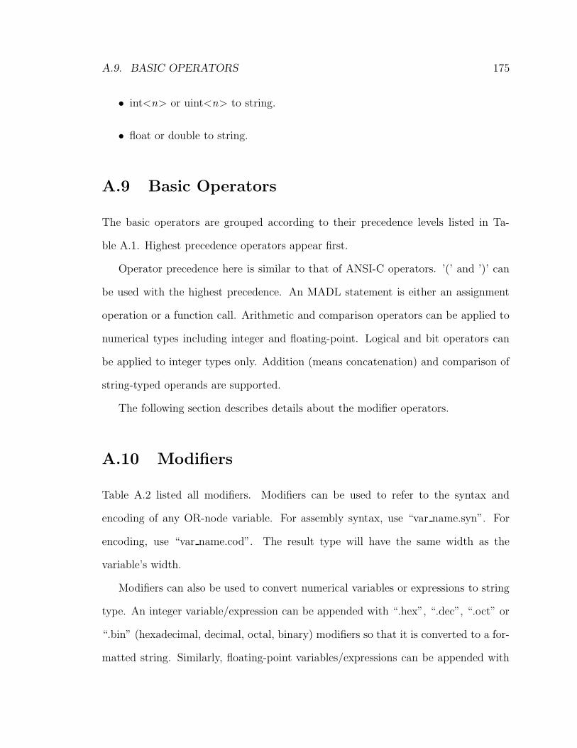
A.9. BASIC OPERATORS 175
• int<n> or uint<n> to string.
• float or double to string.
A.9 Basic Operators
The basic operators are grouped according to their precedence levels listed in Ta-
ble A.1. Highest precedence operators appear first.
Operator precedence here is similar to that of ANSI-C operators. ’(’ and ’)’ can
be used with the highest precedence. An MADL statement is either an assignment
operation or a function call. Arithmetic and comparison operators can be applied to
numerical types including integer and floating-point. Logical and bit operators can
be applied to integer types only. Addition (means concatenation) and comparison of
string-typed operands are supported.
The following section describes details about the modifier operators.
A.10 Modifiers
Table A.2 listed all modifiers. Modifiers can be used to refer to the syntax and
encoding of any OR-node variable. For assembly syntax, use “var name.syn”. For
encoding, use “var name.cod”. The result type will have the same width as the
variable’s width.
Modifiers can also be used to convert numerical variables or expressions to string
type. An integer variable/expression can be appended with “.hex”, “.dec”, “.oct” or
“.bin” (hexadecimal, decimal, octal, binary) modifiers so that it is converted to a for-
matted string. Similarly, floating-point variables/expressions can be appended with
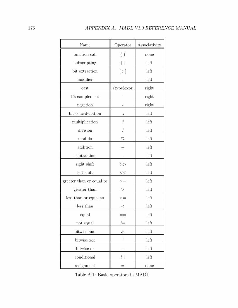
176 APPENDIX A. MADL V1.0 REFERENCE MANUAL
Name Operator Associativity
function call ( ) none
subscripting [ ] left
bit extraction [ : ] left
modifier . left
cast (type)expr right
1’s complement ˜ right
negation - right
bit concatenation :: left
multiplication * left
division / left
modulo % left
addition + left
subtraction - left
right shift >> left
left shift << left
greater than or equal to >= left
greater than > left
less than or equal to <= left
less than < left
equal == left
not equal != left
bitwise and & left
bitwise xor ˆ left
bitwise or — left
conditional ? : left
assignment = none
Table A.1: Basic operators in MADL
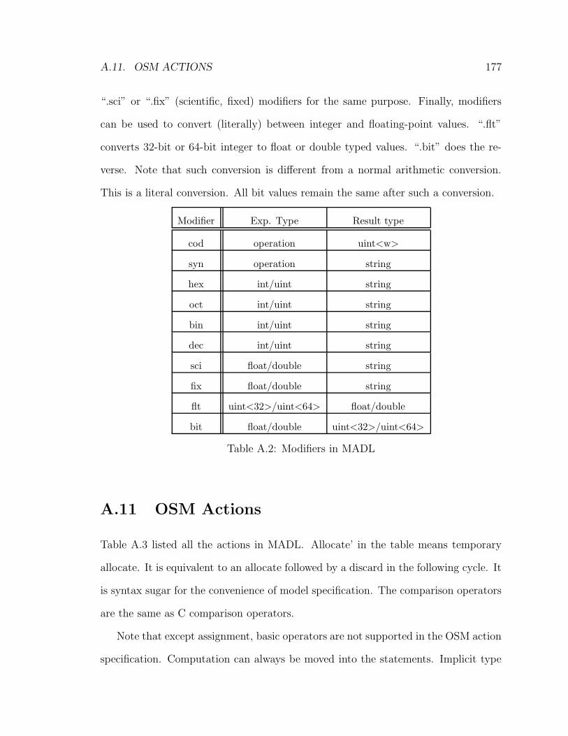
A.11. OSM ACTIONS 177
“.sci” or “.fix” (scientific, fixed) modifiers for the same purpose. Finally, modifiers
can be used to convert (literally) between integer and floating-point values. “.flt”
converts 32-bit or 64-bit integer to float or double typed values. “.bit” does the re-
verse. Note that such conversion is different from a normal arithmetic conversion.
This is a literal conversion. All bit values remain the same after such a conversion.
Modifier Exp. Type Result type
cod operation uint<w>
syn operation string
hex int/uint string
oct int/uint string
bin int/uint string
dec int/uint string
sci float/double string
fix float/double string
flt uint<32>/uint<64> float/double
bit float/double uint<32>/uint<64>
Table A.2: Modifiers in MADL
A.11 OSM Actions
Table A.3 listed all the actions in MADL. Allocate’ in the table means temporary
allocate. It is equivalent to an allocate followed by a discard in the following cycle. It
is syntax sugar for the convenience of model specification. The comparison operators
are the same as C comparison operators.
Note that except assignment, basic operators are not supported in the OSM action
specification. Computation can always be moved into the statements. Implicit type
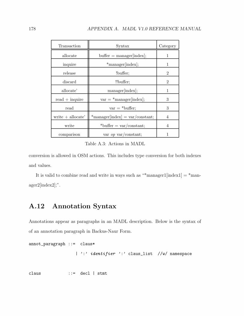
178 APPENDIX A. MADL V1.0 REFERENCE MANUAL
Transaction Syntax Category
allocate buffer = manager[index]; 1
inquire *manager[index]; 1
release !buffer; 2
discard !!buffer; 2
allocate’ manager[index]; 1
read + inquire var = *manager[index]; 3
read var = *buffer; 3
write + allocate’ *manager[index] = var/constant; 4
write *buffer = var/constant; 4
comparison var op var/constant; 1
Table A.3: Actions in MADL
conversion is allowed in OSM actions. This includes type conversion for both indexes
and values.
It is valid to combine read and write in ways such as “*manager1[index1] = *man-
ager2[index2];”.
A.12 Annotation Syntax
Annotations appear as paragraphs in an MADL description. Below is the syntax of
of an annotation paragraph in Backus-Naur Form.
annot_paragraph ::= claus*
| ’:’ identifier ’:’ claus_list //w/ namespace
claus ::= decl | stmt
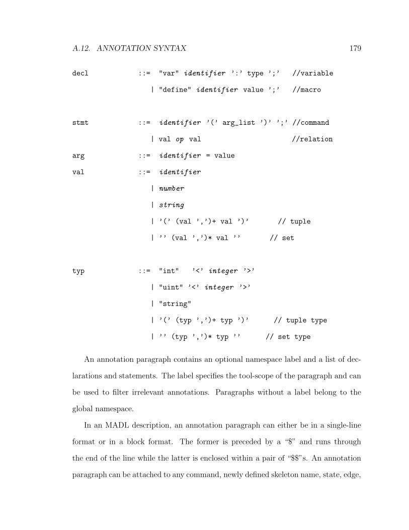
A.12. ANNOTATION SYNTAX 179
decl ::= "var" identifier ’:’ type ’;’ //variable
| "define" identifier value ’;’ //macro
stmt ::= identifier ’(’ arg_list ’)’ ’;’ //command
| val op val //relation
arg ::= identifier = value
val ::= identifier
| number
| string
| ’(’ (val ’,’)+ val ’)’ // tuple
| ’’ (val ’,’)* val ’’ // set
typ ::= "int" ’<’ integer ’>’
| "uint" ’<’ integer ’>’
| "string"
| ’(’ (typ ’,’)+ typ ’)’ // tuple type
| ’’ (typ ’,’)* typ ’’ // set type
An annotation paragraph contains an optional namespace label and a list of dec-
larations and statements. The label specifies the tool-scope of the paragraph and can
be used to filter irrelevant annotations. Paragraphs without a label belong to the
global namespace.
In an MADL description, an annotation paragraph can either be in a single-line
format or in a block format. The former is preceded by a “$” and runs through
the end of the line while the latter is enclosed within a pair of “$$”s. An annotation
paragraph can be attached to any command, newly defined skeleton name, state, edge,

180 APPENDIX A. MADL V1.0 REFERENCE MANUAL
variable, buffer, manager class, manager instance, syntax operation name, function
name, statement, action, SYNTAX subsection, CODING subsection, and edge name
reference in TRANS subsection.
References
[1] Advanced RISC Machines Ltd. ARM Architecture Reference Manual, 1996.
[2] H. Akaboshi. A Study on Design Support for Computer Architecture Design. PhD
thesis, Department of Information Systems, Kyushu University, Japan, 1996.
[3] D. I. August, D. A. Connors, S. A. Mahlke, J. W. Sias, K. M. Crozier, B. Cheng,
P. R. Eaton, Q. B. Olaniran, and W. W. Hwu. Integrated predicated and specula-
tive execution in the IMPACT EPIC architecture. In Proceedings of International
Symposium on Computer Architecture, pages 227–237, 1998.
[4] T. Austin, E. Larson, and D. Ernst. SimpleScalar: An infrastructure for com-
puter system modeling. IEEE Computer, pages 59–67, Feb 2002.
[5] AXYS Design Automation, Inc. http://www.axysdesign.com (current July
2004).
[6] G. Baldwin, K. Keutzer, and R. Newton. The MARCO/DARPA Gigascale Sili-
con Research Center introduction and overview, Presentation in the GSRC An-
nual Review, December 2000.
[7] Bluespec, Inc. http://www.bluespec.com (current July 2004).
181
182 APPENDIX A. REFERENCES
[8] D. G. Bradlee, R. R. Henry, and S. J. Eggers. The Marion system for retargetable
instruction scheduling. In Proceedings of the Conference on Programming Lan-
guage Design and Implementation, June 1991.
[9] F. Burns, A. Koelmans, and A. Yakovlev. Modelling of superscalar processor
architectures with design/CPN. In Proceedings of Workshop on Practical Use of
Coloured Petri Nets and Design, June 1998.
[10] K. Cheng and A. S. Krishnakumar. Automatic generation of functional vectors
using the extended finite state machine model. ACM Transactions on Design
Automation of Electronic Systems, 1(1):57–79, 1 1996.
[11] P. S. Coe, F. W. Howell, R. N. Ibbett, and L. M. Williams. Technical note:
A hierarchical computer architecture design and simulation environment. ACM
Transactions on Modeling and Computer Simulation, pages 431–446, Oct 1998.
[12] Compaq Computer Corporation. iPAQ H3000 Pocket PC Reference Guide, 2000.
[13] T. M. Conte, M. A. Hirsch, and K. N. Menezes. Reducing state loss for effec-
tive trace sampling of superscalar processors. In Proceedings of International
Conference on Computer Design, pages 468–477, 1996.
[14] T. M. Cover and J. A. Thomas. Elements of information theory. Wiley, New
York, 1991.
[15] CoWare, Inc. http://www.coware.com (current July 2004).
[16] W. L. A. de Oliveira, N. Marranghello, and F. Damiani. Modeling a processor
with a Petri Net extension for digital systems. In Proceedings of the Conference
on Design, Analysis, and Simulation of Distributed Systems, 2004.
183
[17] S. A. Edwards. The specification and execution of heterogeneous synchronous
reactive systems. PhD thesis, University of California at Berkeley, Berkeley, CA,
1998.
[18] J. Emer, P. Ahuja, E. Borch, A. Klauser, C.-K. Luk, S. Manne, S. S. Mukherjee,
H. Patil, S. Wallace, N. Binkert, R. Espasa, and T. Juan. Asim: A performance
model framework. IEEE Computer, pages 68–76, February 2002.
[19] A. Fauth, J. V. Praet, and M. Freericks. Describing instructions set processors
using nML. In Proceedings of Conference on Design Automation and Test in
Europe, pages 503–507, Paris, France, 1995.
[20] Free Software Foundation. http://www.gnu.org/software/gdb/gdb.html
(current July 2004).
[21] Free Software Foundation. Using the GNU Compiler Collection, http://gcc.
gnu.org/onlinedocs/gcc-3.4.0/gcc (current july 2004).
[22] Fujitsu Ltd. Hiperion II - Digital Signal Processor User’s Manual, 1998.
[23] B. Fuller. Intel CTO says chip design needs rethinking, EETimes, June 2004.
[24] T. Grotker, S. Liao, G. Martin, and S. Swan. System Design with SystemC.
Kluwer Academic Publishers, Boston, MA, 2002.
[25] J. C. Gyllenhaal, W. Hwu, and B. R. Rao. HMDES version 2.0 specification.
Technical Report IMPACT-96-3, University of Illinois at Urbana-Champaign,
1996.
184 APPENDIX A. REFERENCES
[26] G. Hadjiyiannis, S. Hanono, and S. Devadas. ISDL: An instruction set description
language for retargetability. In Proceedings of Design Automation Conference,
pages 299–302, June 1997.
[27] G. Hadjiyiannis, P. Russo, and S. Devadas. A methodology for accurate perfor-
mance evaluation in architecture exploration. In Proceedings of Design Automa-
tion Conference, pages 927–932, 1999.
[28] A. Halambi, P. Grun, V. Ganesh, A. Khare, N. Dutt, and A. Nicolau. EXPRES-
SION: A language for architecture exploration through compiler/simulator re-
targetability. In Proceedings of Conference on Design Automation and Test in
Europe, pages 485–490, 1999.
[29] D. Harel. Statecharts: A visual formalism for complex systems. Science of
Computer Programming, 8(3):231–274, June 1987.
[30] R. Harper. Programming Languages: Theory and Practice (draft), 2002.
[31] J. W. Haskins and K. Skadron. Minimal subset evaluation: Rapid warm-up
for simulated hardware state. In Proceedings of International Conference on
Computer Design, pages 32–39, 2001.
[32] J. C. Hoe and Arvind. Synthesis of operation-centric hardware descriptions. In
Proceedings of International Conference on Computer-aided Design, pages 511–
519, 2000.
[33] D. A. Huffman. A method for the construction of minimum redundancy codes.
Proceedings of the Institute of Radio Engineers, 40:1098–1101, 1952.
185
[34] IEEE Inc., 3 Park Avenue, New York, NY 10016-5997, USA. IEEE Standard
VHDL Language Reference Manual (1076-2000), 2000.
[35] IEEE Inc., 3 Park Avenue, New York, NY 10016-5997, USA. IEEE Standard
Hardware Description Language Based on the Verilog Hardware Description Lan-
guage (1364-2001), 2001.
[36] Improv Systems, Inc. http://www.improvsys.com (current July 2004).
[37] Intel Corporation. Moore’s Law, http://www.intel.com/research/silicon/
mooreslaw.htm (current July 2004).
[38] Intel Corporation. Intel StrongARM SA-1110 Microprocessor Developer’s Man-
ual, 2001.
[39] International Business Machines Corporation. PowerPC Microprocessor Family:
The Programming Environments for 32-bit Microprocessors, 2000.
[40] D. Kastner. Retargetable Postpass Optimization by Integer Linear Programming.
PhD thesis, Saarland University, Germany, 2000.
[41] H. Kaul and D. Sylvester. Future performance challenges in nanometer design.
In Proceedings of Design Automation Conference, pages 3–8, 2001.
[42] N. S. Kim, T. Austin, D. Blaauw, T. Mudge, K. Flautner, J. Hu, M. J. Irwin,
M. Kandemir, and V. Narayanan. Leakage current : Moore’s law meets static
power. IEEE Computer, 36(12):68–75, 12 2003.
[43] D. E. Knuth. The Art of Computer Programming, Vol.3:Searching and Sorting.
Addison-Wesley, Reading, MA, 1973.
186 APPENDIX A. REFERENCES
[44] M. Lapedus. IC makers brace for $3 million mask at 65nm, EETimes, September
2003.
[45] C. Lee, M. Potkonjak, and W. H. Mangione-Smith. MediaBench: A tool for eval-
uating and synthesizing multimedia and communicatons systems. In Proceedings
of International Symposium on Microarchitecture, pages 330–335, 1997.
[46] R. B. Lee and A. M. Fiskiran. PLX: A fully subword-parallel instruction set
architecture for fast scalable multimedia processing. In Proceedings of the 2002
IEEE International Conference on Multimedia and Expo (ICME 2002), pages
117–120, August 2002.
[47] R. Leupers and P. Marwedel. Retargetable generation of code selectors from
HDL processor models. In Proceedings of Conference on Design Automation and
Test in Europe, pages 140–144, 1997.
[48] The Liberty Research Group. Liberty Simulation Environment Developers Man-
ual, 1.0 edition.
[49] J. Matthews, B. Cook, and J. Launchbury. Microprocessor specification in Hawk.
In Proceedings of the International Conference on Computer Languages, pages
90–101, 1998.
[50] P. Mishra, N. Dutt, and A. Nicolau. Functional abstraction driven design space
exploration of heterogeneous programmable architectures. In Proceedings of the
International Symposium on System Synthesis, pages 256–261, Oct 2001.
[51] W. S. Mong and J. Zhu. A retargetable micro-architecture simulator. In Pro-
ceedings of Design Automation Conference, pages 752–757, 2003.

187
[52] B. M. E. Moret. Decision trees and diagrams. ACM Computing Surveys,
14(4):593–623, 1982.
[53] G. Mouchard. http://www.microlib.org (current July 2004).
[54] H. Muljono, S. Rusu, B. Cherkauer, and J. Stinson. Two new 130nm Itanium 2
processors for 2003. In HOT Chips 15 Proceedings, 2003.
[55] T. Murata. Petri Nets: Properties, analysis and applications. Proceedings of the
IEEE, 77(4):541–580, 4 1989.
[56] S. K. Murthy. Automatic construction of decision trees from data: A multi-
disciplinary survey. Data Mining and Knowledge Discovery, 2(4):345–389, 1998.
[57] A. Nohl, G. Braun, O. Schliebusch, R. Leupers, H. Meyr, and A. Hoffmann. A
universal technique for fast and flexible instruction-set architecture simulation.
In Proceedings of Design Automation Conference, pages 22–27, 2002.
[58] NVIDIA Corporation. http://www.nvidia.com/page/geforce_6800.html
(current July 2004).
[59] Object Management Group, Inc. OMG-Unified Modeling Language Specification,
1.5 edition, March 2003.
[60] S. Onder and R. Gupta. Automatic generation of microarchitecture simulators.
In Proceedings of the IEEE International Conference on Computer Languages,
pages 80–89, May 1998.
[61] S. C. Park. High-end design verification, Presentation in AP-SoC 2003, Novem-
ber 2003.
188 APPENDIX A. REFERENCES
[62] D. A. Patterson and J. L. Hennessy. Computer Architecture: A Quantitative
Approach. Morgan Kaufmann Publishers, San Francisco, CA, 2nd edition, 1996.
[63] R. W. Payne and D. A. Preece. Identification keys and diagnostic tables: A
review. Journal of the Royal Statistics Society, Series A, 143(3):253–292, 1980.
[64] S. Pees, A. Hoffmann, V. Zivojnovic, and H. Meyr. LISA – machine descrip-
tion language for cycle-accurate models of programmable DSP architectures. In
Proceedings of Design Automation Conference, pages 933–938, 1999.
[65] L. Pileggi, H. Schmit, A. J. Strojwas, P. Gopalakrishnan, V. Kheterpal, A. Koora-
paty, C. Patel, V. Rovner, and K. Y. Tong. Exploring regular fabrics to optimize
the performance-cost trade-off, Presentation in the Design Automation Confer-
ence, June 2003.
[66] W. Qin. http://www.princeton.edu/~wqin/armsim.htm (current July 2004).
[67] W. Qin and S. Malik. Architecture description languages for retargetable com-
pilation. In Y. N. Srikant and P. Shankar, editors, Compiler Design Handbook:
Optimizations & Machine Code Generation, pages 535–564. CRC Press, 2002.
[68] W. Qin and S. Malik. Automated synthesis of efficient binary decoders for re-
targetable software toolkits. In Proceedings of Design Automation Conference,
pages 764–769, 2003.
[69] W. Qin and S. Malik. Flexible and formal modeling of microprocessors with
application to retargetable simulation. In Proceedings of Conference on Design
Automation and Test in Europe, pages 556–561, 2003.
189
[70] W. Qin, S. Rajagopalan, and S. Malik. A formal concurrency model based
architecture description language for synthesis of software development tools.
In Proceedings of the ACM SIGPLAN/SIGBED 2004 Conference on Languages,
Compilers, and Tools for Embedded Systems (LCTES’04), June 2004.
[71] W. Qin, S. Rajagopalan, M. Vachharajani, H. Wang, X. Zhu, D. August,
K. Keutzer, S. Malik, and L. Peh. Design tools for application specific embedded
processors. In Proceedings of the ACM International Conference on Embedded
Software, October 2002.
[72] N. Ramsey and J. W. Davidson. Machine descriptions to build tools for embed-
ded systems. In Proceedings of the ACM SIGPLAN Workshop on Languages,
Compilers, and Tools for Embedded Systems, pages 176–192, 1998.
[73] N. Ramsey and M. Fernandez. The New Jersey Machine-Code Toolkit. In Pro-
ceedings of the 1995 USENIX Technical Conference, pages 289–302, January
1995.
[74] S. Rigo, R. J. Azevedo, and G. Araujo. The ArchC architecture description
language. Technical Report 15, Institute of Computing of the University of
Campinas, Brazil, 2003.
[75] C. E. Shannon. A mathematical theory of communication. Bell System Technical
Journal, 27:379–423, 623–656, July, October 1948.
[76] C. Siska. A processor description language supporting retargetable multi-pipeline
DSP program development tools. In Proceedings of the International Symposium
on System Synthesis, pages 31–36, 1998.
190 APPENDIX A. REFERENCES
[77] C. Souza. Semiconductor IP houses struggle to survive as ASIC design starts con-
tinue to dwindle, http://www.my-esm.com/showArticle.jhtml?articleID=
10100072 (current July 2004), May 2003.
[78] SPARC International Inc. The SPARC Architecture Manual, Version 8, 1992.
[79] Standard Performance Evaluation Corporation. http://www.specbench.org
(current July 2004).
[80] A. Sudarsanam. Code optimization libraries for retargetable compilation for em-
bedded digital signal processors. PhD thesis, Princeton University, 1998.
[81] SystemC Community. http://www.systemc.org (current July 2004).
[82] Target Compiler Technologies N.V. http://www.retraget.com (current July
2004).
[83] J. Teich, R. Weper, D. Fischer, and S. Trinkert. A joined architecture/compiler
environment for ASIPs. In Proceedings of International Conference on Compil-
ers, Architectures and Synthesis for Embedded Systems, pages 26–33, San Jose,
CA, Nov 2000.
[84] Tensilica, Inc. http://www.tensilica.com (current July 2004).
[85] A. Terechko, E. Pol, and J. van Eijndhoven. PRMDL: A machine description
language for clustered VLIW architectures. In Proceedings of Conference on
Design Automation and Test in Europe, page 821, 2001.
[86] Texas Instrument Inc. TMS320C6000 CPU and Instruction Set Reference Guide,
2000.
191
[87] The Free Software Foundation. http://www.gnu.org (current July 2004).
[88] The Ptolemy Project. http://ptolemy.eecs.berkeley.edu (current July
2004).
[89] H. Theiling. Generating decision trees for decoding binaries. ACM SIGPLAN
Notices, 36(8):112–120, 2001.
[90] H. Tomiyama, A. Halambi, P. Grun, N. Dutt, and A. Nicolau. Architecture
description languages for system–on–chip design. In Proceedings of The Sixth
Asia Pacific Conference on Chip Design Language (APCHDL), 1999.
[91] J. Turley. The two percent solution, http://www.embedded.com/shared/
printableArticle.jhtml?articleID=9900861 (current july 2004), December
2002.
[92] M. Vachharajani, N. Vachharajani, D. Penry, J. A. Blome, and D. I. August. Mi-
croarchitectural exploration with Liberty. In Proceedings of International Sym-
posium on Microarchitecture, pages 271–282, Nov 2002.
[93] A. S. Vincentelli. Defining platform-based design, EEDesign of EETimes, Febru-
ary 2002.
[94] A. Wang, E. Killian, D. Maydan, and C. Rowen. Hardware/software instruc-
tion set configurability for system-on-chip processors. In Proceedings of Design
Automation Conference, pages 184–188, 2001.
[95] R. E. Wunderlich, T. F. Wenisch, B. Falsafi, and J. C. Hoe. SMARTS: Accelerat-
ing microarchitecture simulation via rigorous statistical sampling. In Proceedings
of International Symposium on Computer Architecture, pages 84–97, 2003.
192 APPENDIX A. REFERENCES
[96] G. Zimmerman. The MIMOLA design system: A computer-aided processor
design method. In Proceedings of Design Automation Conference, pages 53–58,
June 1979.
[97] V. Zivojinovic, J. M. Velarde, C. Schlager, and H. Meyr. DSPStone: A DSP-
oriented benchmarking methodology. In Proceedings of International Conference
of Signal Processing Application Technology, pages 715–720, October 1994.
[98] W. M. Zuberek, R. Govindarajan, and F. Suciu. Timed Colored Petri Net models
of distributed memory multithreaded processors. In Proceedings of Workshop on
Practical Use of Coloured Petri Nets and Design, June 1998.