Model predictive control relevant identification and validation

Chemical Engineering Science 58 (2003) 2389–2401www.elsevier.com/locate/ces

Model predictive control relevant identi#cation and validation

Biao Huanga ;∗, Ashish Malhotraa, Edgar C. Tamayob

aDepartment of Chemical and Materials Engineering, University of Alberta, Edmonton, AB, Canada T6G 2G6bSyncrude Canada Ltd., P.O. Bag 4009, Fort McMurray, AB, Canada T9H 3L1

Received 1 January 2002; accepted 7 December 2002

Abstract

The role of data pre#ltering in model identi#cation and validation is presented in this paper. A model predictive control relevant datapre#lter, namely the multistep ahead prediction #lter for optimal predictions over every step within a #nite horizon, is presented. It is shownthat models that minimize the multistep prediction errors can be identi#ed or veri#ed by #ltering the data using certain data pre#lters andthen applying the prediction error method to the #ltered data. Based on these identi#cation results, a predictive control relevant modelvalidation scheme using the local approach is proposed. The developed algorithms are veri#ed through simulations as well as industrialapplications.? 2003 Elsevier Science Ltd. All rights reserved.

Keywords: Model validation; Detection of abrupt change; Process identi#cation; Optimal prediction; Prediction error method; Model predictive control

1. Introduction

Motivations. This work is a continuation of the work byHuang and Tamayo (2000) and Huang (2000) and is moti-vated by a commonly observed practical dilemma: It is wellknown that performance of control systems depends heav-ily on the quality of models. This is particularly true formodel predictive control systems which are the most widelyapplied advanced control technology in chemical process.However, it is often observed that many models used in ex-isting model predictive control systems are not able to passa “rigorous” model validation test but the control systemswork #ne. On the other hand, some models, which appar-ently pass the “rigorous” validation test, fail to deliver asatisfactory performance. What is a “good” process model?How should we test it? This question is naturally related tocontrol relevant model identi#cation techniques.Studies on identi#cation have primarily focused on ques-

tions of convergence and e@ciency of parameter and transferfunction estimates in the case when the true system is con-tained in the model set (Ljung, 1999; Soderstrom & Stoica,1989; Bitmead, Gevers, &Wertz, 1990). However, the moretypical case in identi#cation is that of under-modeling or

∗ Corresponding author. Tel.: +1-403-492-9016;fax: +1-403-492-2881.

E-mail address: [email protected] (B. Huang).

identi#cation of reduced-complexity models when the plantis not in the model set (Van den Hof & Schrama, 1995).Under such circumstances, the model-plant mismatch oftenconsists of both bias error (due to under-modeling) and vari-ance error (due to disturbances). Control performance hasto be compromised to accommodate these model uncertain-ties, and direct application of the prediction error method(Ljung, 1999) may not give the best model for control.A control relevant identi#cation scheme that aims at

achieving optimal control performance has been proposedby many researchers (Zang, Bitmead, & Gevers, 1995; Vanden Hof & Schrama, 1995). Control relevant identi#cationis to search for appropriate data pre#lters before applyingthe prediction error method or other identi#cation methodsto the data such that the identi#ed model is most suitablefor the controller design. If a model is expressed in thefrequency domain, then data pre#ltering is equivalent tochanging the weighting on model errors in the identi#cationobjective function. Larger weightings in some frequenciesgenerally result in less error of the model in the corre-sponding frequencies. However, this typically increasesmodel error in some other frequencies and is known asthe water-bed eJect. Therefore, the data pre#lter should bechosen in such a way that it yields the most accurate modelin the frequencies that are critical to control performance.The role of data pre#ltering has been extensively

discussed in the literature. Fundamental theory on data

0009-2509/03/$ - see front matter ? 2003 Elsevier Science Ltd. All rights reserved.doi:10.1016/S0009-2509(03)00077-0

mailto:[email protected]

2390 B. Huang et al. / Chemical Engineering Science 58 (2003) 2389–2401

pre#ltering can be found in the pioneering work of Ljung(1999). Data pre#ltering for the LQG controller design hasbeen discussed by Bitmead et al. (1990), for the long rangepredictive controller design by Shook, Mohtadi, and Shah(1992), for the IMC controller design by Rivera, Pollard,and Garcia (1992) and for the robust control design byCooley and Lee (1998). In addition, subspace identi#ca-tion (Larimore, 1990; Van Overschee & De Moor, 1996;Verhaegen, 1994) uses the prediction #rst and then theprojection algorithm to derive process models and is natu-rally a prediction (or predictive control) relevant approach.Many other control relevant identi#cation algorithms canalso be found in the literature and we will not list all ofthem here.Once a model is identi#ed from the process, it is impor-

tant to have model validation as the last “quality control”station before a model is delivered to the users (Ljung &Guo, 1997). It is equally important to continuously validatethe model even after the model is delivered to the usersand “maintain” the model quality by detecting changes ofthe model parameters. Industries have an increasing need tohave a tool to continuously validate the model and detectchanges for maintaining the model-based control systems.There is a large volume of papers concerned with controlrelevant model identi#cation. There is also a large volumeof papers concerned with ‘rigorous’ model validation in theidenti#cation stage (Ljung, 1999; Sternad & Soderstrom,1988). However, the literature has been relatively sparseon studies concerned with control relevant model validationtechniques in the industrial environments.Model validation is naturally related to detection of

parameter changes. Among various statistical detection al-gorithms, the local approach for detection of abrupt changehas recently regained signi#cant interests due to the notablework of Basseville (1998). The eJectiveness and reliabilityof this approach has been demonstrated by its applicationsin the monitoring of critical processes such as nuclear powerplants, gas turbines, catalytic converter etc. (Basseville,1998; Zhang, Basseville, & Benveniste, 1994). The localapproach has a number of distinct features. Among themare the simplicity yet asymptotically uniformly most pow-erfulness and capability to detect small changes (Basseville,1998). The challenge to local detection approach, however,is the sensitivity issue of the algorithm (Basseville, 1998).The algorithm is sensitive to any small change of modelparameters. This is not desired in practice since not allparameter changes can aJect control performance and needto issue an alarm. The question is how to remain sensitiveto the changes that are “critical” to process performancewhile insensitive to otherwise. This motivates the authorsto develop a detection algorithm that is model predictivecontrol relevant and has a potential to be widely appliedin model validation for model predictive control systems.New residuals that are model predictive control relevant aredeveloped in this paper and are veri#ed through simulationsand industrial applications.

The remaining of this paper is organized as follows: InSection 2, the local approach for detection of abrupt changeis revisited. In Section 3, the local approach is applied tothe prediction error method to derive a one-step predictionrelevant model validation algorithm. In Sections 4 and 5,the one-step prediction relevant validation technique is ex-tended to k-step and multistep prediction relevant validationalgorithms, respectively. Simulation examples are given inSection 6. Industrial application examples are reported inSection 7, followed by concluding remarks in Section 8.

2. Local approach for detection of abrupt changes

2.1. Detection problem

Basseville (1998) has developed a procedure for the de-tection of abrupt parameter change and isolation of thechanging parameters. The results are summarized in thissection. For detailed mathematical derivation, readers arereferred to Basseville (1998) and Zhang, Basseville, andBenveniste (1998).For a process model

yt = Gput + GLat;

where the process and disturbance models Gp and GL areparameterized by . Assume that parameters before changeare given by 0, and after change given by 0+�=

√N where

� is a vector with the same dimension as 0 but with asmall magnitude. The detection of abrupt change can beformulated as the following hypothesis test problem:

H0 : = 0 versus H1 : = 0 +1√N

�:

A statistic �N () given by

�N () =1√N

N∑t=1

H (zt ; )

is de#ned as a normalized residual if

E[H (zt ; )] = 0 for = 0 (1)

and

E[H (zt ; )] �= 0 for ∈!(0) \ 0; (2)

where !(0)\0 reads as a neighborhood of 0 exclusive of0. H (zt ; ) is de#ned as the primary residual (Basseville,1998), where zt = [ut ; yt]T. Note that the residuals de#nedhere are diJerent from the regular residuals de#ned in mostof the model identi#cation literatures, and are asymptoticallysu@cient statistics (Basseville, 1998). The empirical versionof Eqs. (1) and (2) may be written as

1N

N∑t=1

H (zt ; ) = 0 for = 0 (3)

and

1N

N∑t=1

H (zt ; ) �= 0 for ∈!(0) \ 0: (4)

B. Huang et al. / Chemical Engineering Science 58 (2003) 2389–2401 2391

If we can #nd such residuals, then for su@cient large N , thefollowing results hold:

�N (0) ∼ N (0; �(0)) under H0;

�N (0) ∼ N (−M (0)�; �(0)) under H1;

where

M (0) = E(

@@

H (zt ; )|=0

); (5)

�(0) =∞∑

t=−∞Cov(H (z1; 0); H (zt ; 0)): (6)

In practice, the empirical version of Eq. (5) may be writtenas

M (0) ≈ @@

[1N

N∑t=1

H (zt ; )

]=0

(7)

and �(0) may be approximated (Zhang et al., 1998) by

�(0)≈ 1N

N∑t=1

H (zt ; 0)HT(zt ; 0)

+I∑

i=1

1N − i

N−i∑t=1

(H (zt ; 0)HT(zt+i ; 0)

+H (zt+i ; 0)HT(zt ; 0)); (8)

where the value I should be properly selected according tothe correlation of the signals. In practice, one can graduallyincrease the value of I until �(0) converges. With theseresults, detection of small changes in the parameter isasymptotically equivalent to the detection of the changes inthe mean of a Gaussian vector. The generalized likelihoodratio (GLR) test detecting unknown changes in the mean ofa Gaussian vector is a �2 test. It is shown (Basseville, 1998)that the GLR test of H1 against H0 can be written as

�2global = �N (0)T�−1(0)M (0)

×(MT(0)�−1(0)M (0))−1

×MT(0)�−1(0)�N (0): (9)

If M (0) is a square matrix, then this test can further besimpli#ed to

�2global = �N (0)T�−1(0)�N (0): (10)

�2global has a central �2 distribution under H0, and a noncentral

�2 distribution under H1. The degree of freedom of �2global isthe row dimension of . A threshold value �2� can be foundfrom a �2 table, where � is the false alarm rate speci#ed bythe users. If �2global is found to be larger than the thresholdvalue, then a change in the parameter is detected.

2.2. Isolation problem

Once a change is detected from the model parameters, itis often desired to isolate which or which sets of parame-ters have changed. This is known as the isolation problem(Basseville, 1998). Partition into a and b, and � into �a

and �b accordingly. The isolation problem can be formulatedas the following hypotheses test:

H0 : �a = 0 versus H1 : �a �= 0: (11)

This test reads as “no changes of parameters in the set of a

versus changes of parameters in the set of a”.Two tests have been recommenced. By assuming �b = 0,

the test (11) is called the sensitivity test. If �b is treated asnuisances, i.e. �b is not necessarily zero, then the test (11)is called the minmax test.Partition the matrix M (0) into two matrices

M (0) = [Ma;Mb]

which corresponds to the partition of , i.e. the column di-mension of Ma is the same as the row dimension of a andthe column dimension of Mb is the same as the row dimen-sion of b. Then the sensitivity test can be written as

�2a = �TaF−1aa �a; (12)

where

�a =MTa �

−1(0)�N (0);

Faa =MTa �

−1(0)Ma;

and �2a has a �2 distribution with na degrees of freedom.

To perform the minmax test, de#ne

F =MT(0)�−1(0)M (0)

and partition it to

F =

[Faa Fab

Fba Fbb

]=

[MT

a �−1(0)Ma MT

a �−1(0)Mb

MTb �

−1(0)Ma MTb �

−1(0)Mb

]:

De#ne

�a =MTa �

−1(0)�N (0);

�b =MTb �

−1(0)�N (0)

and

�∗a = �a − FabF−1bb �b;

F∗a = Faa − FabF−1

bb Fba:

Then the minmax test can be written as

�2∗a = �∗Ta F∗−1a �∗a ; (13)

where �2∗a has a �2 distribution with na degrees of freedom.

By comparing �2∗a with a prespeci#ed threshold, onecan determine whether the parameters in a have changed.The alternative practical method recommended by Zhanget al. (1998) is to compute a minmax test for each possible


sub-vector �a. Among all these minmax tests, the one hav-ing the largest value indicates the nonzero sub-vector �a. Anobvious advantage of this approach is that no threshold isneeded. The downside is that it involves a signi#cant com-putation eJort.Although the mathematical foundation is laid here for de-

tection of abrupt change using the local approach, the chal-lenge in practice is to #nd appropriate normalized residualsand primary residuals that are capable of detecting smallchanges while robust to changes that are irrelevant to cer-tain performance objectives. Dealing with the challenge isthe objective of this paper as will be discussed in the fol-lowing sections.

3. Model validation for optimal one-step ahead prediction

Every model is built to serve for a certain purpose. Mod-eling error almost always exists. It is a common sense that amodel is valid as long as the modeling error does not aJectthe model to serve for its intended “purpose”. The objectiveof the following three sections is to derive validation algo-rithms to monitor whether the model can serve for its in-tended purpose. In this section, the purpose of the modelingis assumed to be optimal one-step ahead prediction.Ljung (1999) has shown that for the general Box–Jenkins

model

yt = Gput + GLat; (14)

where Gp and GL are process and disturbance transferfunctions, respectively, and at is white noise, the optimalone-step ahead predictor is given by

yt|t−1 = G−1L Gput + (1− G−1

L )yt: (15)

Note that Gp and GL are not known in general. If the esti-mated models Gp and GL are used, then the estimated opti-mal predictor may be written as

y t|t−1 = G−1L Gput + (1− G−1

L )yt: (16)

The one-step ahead prediction error is given by

�t|t−1 = yt − y t|t−1;

=1

GL[Gp; GL]

[ut

at

];

where Gp = Gp − Gp. Consider an objective function

J =1N

N∑t=1

�2t|t−1 (17)

which is sum of squares of one-step ahead prediction er-ror. When N is su@ciently large, this objective can be

approximated by

J = E[�2t|t−1]:

It follows from the Parseval’s Theorem that

E[�2t|t−1] =12

∫

−

1

|GL(ej!)|2[Gp(ej!) GL(ej!)]

×[

!u(!) !ua(!)

!au(!) "2a

][Gp(e−j!)

GL(e−j!)

]d!:

(18)

The optimal estimates, Gp and GL, that minimize the pre-diction error may be obtained by minimizing this predictionerror equation, i.e.

[Gp; GL] = argmin12

∫

−

1

|GL(ej!)|2[Gp(ej!) GL(ej!)]

×[

!u(!) !ua(!)

!au(!) "2a

][Gp(e−j!)

GL(e−j!)

]d!:

(19)

This is known as the prediction error method for model iden-ti#cation. One can see, from the derivation, that estimatesobtained from the prediction error method should give thebest one-step ahead prediction.Now let us parameterize a process model by

yt =Gput + GLat

=B(q−1)F(q−1)

ut +C(q−1)D(q−1)

at ; (20)

where

B(q−1) = b1q−1 + · · ·+ bnbq−nb ;

F(q−1) = f1q−1 + · · ·+ fnfq−nf ;

C(q−1) = c1q−1 + · · ·+ cncq−nc ;

D(q−1) = d1q−1 + · · ·+ dndq−nd :

The parameter of interest, , is given by

= [ b1 · · · bnb f1 · · · fnf c1 · · · cnc d1 · · · dnd ]T:

Model validation is equivalent to the detection of parame-ter changes (Benveniste, Basseville, & Moustakides, 1987).The objective of this section is to derive a local detectionalgorithm that is relevant to the objective. That is, the de-tection algorithm should only be sensitive to the parameterchanges that can aJect the one step ahead prediction.For the sake of convenience, de#ne the following new

one-step prediction error objective function:

J =1N

N∑t=1

12�2t|t−1 (21)


which is equivalent to Eq. (17), where �t|t−1 is the one stepahead prediction error given by

�t|t−1 = yt − y t|t−1

and y t|t−1 is the one step ahead prediction given by

y t|t−1 =(D(q−1)C(q−1)

)B(q−1)F(q−1)

ut +(1− D(q−1)

C(q−1)

)yt:

The gradient of Eq. (21) can be calculated as

@J@=− 1

N

N∑t=1

(@�t|t−1@

)T�t|t−1: (22)

Assume that 0 is calculated by equating Eq. (22) to zero.Then the estimation 0 based on the prediction error methodthat minimizes Eq. (21) must satisfy

@J@

∣∣∣∣0

=−[1N

N∑t=1

(@�t|t−1@

)T�t|t−1

]=0

= 0: (23)

As the sample size increases, Eq. (23) is asymptoticallyequivalent to

E

[(@�t|t−1@

)T�t|t−1

]=0

= 0: (24)

Obviously, for any new data generated from Eq. (20), if = 0, then Eq. (24) should continue to hold. If, on theother hand, �= 0 then Eq. (24) will be nonzero. Hence, themodel validation problem is reduced to that of monitoringthe mean of a vector which is given by

H (zt ; ) =(@�t|t−1@

)T�t|t−1: (25)

This is exactly the primary residual as de#ned in Eqs. (1)and (2). The actual monitoring can be done by performinga �2 test on the normalized residual given by

�N () =1√N

N∑t=1

H (zt ; ): (26)

To calculate the primary residual, the partial derivative ofthe prediction error needs to be calculated #rst. The partialderivative of the prediction errors can be calculated as(

@�t|t−1@

)=(@y t|t−1

@

)= (t; ); (27)

where

(t; ) =@y t|t−1

@

=[

@@bk

y t|t−1@@ck

y t|t−1@

@dky t|t−1

@@fk

y t|t−1

]T:

(28)

The partial derivatives of y t|t−1 with respect to the pa-rameters can be evaluated from Eq. (20) as (Ljung, 1999)

@@bk

y t|t−1 =− D(q−1)C(q−1)F(q−1)

ut−k ;

@@ck

y t|t−1 =− D(q−1)B(q−1)C(q−1)C(q−1)F(q−1)

ut−k

+D(q−1)

C(q−1)C(q−1)yt−k ;

@@dk

y t|t−1 =− B(q−1)C(q−1)F(q−1)

ut−k − 1C(q−1)

yt−k ;

@@fk

y t|t−1 =− D(q−1)B(q−1)C(q−1)F(q−1)F(q−1)

ut−k :

For the case of an output error (OE) model

yt =B(q−1)F(q−1)

+ vt ;

where the disturbance model is not parameterized, the ex-pression for (t; ) reduces to

(t; ) =,(t; )F(q−1)

; (29)

where

,(t; )

=[ ut−1 · · · ut−nb − y t−1|t · · · − y t−nf|t−nf+1 ]T:(30)

Therefore, the primary residual for the PEM case is

H (zt ; ) = (t; 0)�t|t−1 (31)

and for the OE case where C(q−1) and D(q−1) are notparameterized becomes

H (zt ; ) =,(t; 0)F(q−1)

�t|t−1: (32)

In many applications, it may be desired that the model val-idation algorithm should not give an alarm if parameterchanges occur only in the disturbance models. Huang (2000)has demonstrated that by associating the detection algorithmwith the output error method, the model validation algorithmbased on the local approach is disturbance model indepen-dent. We shall call this method as the output error method(OEM) based local approach.To summarize, model validation can be performed using

the following algorithm:

Algorithm 1. Provided that model parameter 0 is iden-ti8ed from a set of identi8cation data, a set of vali-dation data can then be used to perform the following


model validation test:

(1) Calculate the primary residualH (zt ; 0) using Eq. (31)or Eq. (32).

(2) Calculate the normalized residual �N (0) usingEq. (26).

(3) Calculate the covariance matrix �(0) using Eq. (8).(4) Calculate �2global using (10).(5) Select the threshold value from the �2 table according

to a prespeci8ed false alarm rate with the degree offreedom being equal to the row dimension of .

(6) If �2global is larger than the threshold, issue an alarmand perform the isolation test; otherwise conclude thatthe model passes the validation test.

Remark 1. There are two scenarios that may be resultedfrom this test, namely model validation and model changedetection. If 0 is treated as a set of parameters to be vali-dated, then this test falls in the category of model validation.In this case, failure of the test means that 0 is falsi#ed bythe validation data. On the other hand, if 0 is treated as aset of initial parameters, then this test falls in the categoryof detection of model changes. Failure of the test meansthat the model parameters have deviated from the initialvalues.

This method will validate model parameters that aJectthe one-step ahead prediction. The result can be extended tomodel validation algorithms for k-step ahead and multistepahead prediction. This is discussed next.

4. Model validation for optimal k-step ahead prediction

Eq. (16) can be extended to the k-step ahead prediction(Ljung, 1999):

y t|t−k = W kGput + (1− W k)yt; (33)

where

W k = Fk G−1L (34)

and

Fk =k−1∑i=0

g(i)q−i ; (35)

where g(i) is the impulse response coe@cient of GL. Thek-step ahead prediction error is given by

�t|t−k = yt − y t|t−k

= W k(yt − Gput)

=Fk

GL[(Gp − Gp)ut + GLat)]: (36)

Following the same procedure as the derivation ofEq. (19), the estimates, Gp and GL, that minimize thek-step ahead prediction error, can be derived as

[Gp; GL] = argmin12

∫

−

|Fk(ej!)|2|GL(ej!)|2

[Gp(ej!) GL(ej!)]

×[

!u(!) !ua(!)

!au(!) "2a

][Gp(e−j!)

GL(e−j!)

]d!:

(37)

Similarly, the estimates calculated by minimizing thek-step ahead prediction error should give the best k-stepprediction. If we #lter yt and ut by Fk and denote the #l-tered data as yf

t and uft , then the one-step ahead predictor

of yft (by #xing the noise model as GL) is given by

yft|t−1 = G−1

L Gpuft + (1− G−1

L )yft :

The one-step ahead prediction error of yft is therefore

given by

�ft|t−1 = yft − yf

t

=1

GL(yf

t − Gpuft )

=Fk

GL(yt − Gput)

=Fk

GL[(Gp − Gp)ut + GLat)];

which is the same as Eq. (36), i.e. k-step ahead predictionerror is the same as one-step ahead prediction error of the#ltered data. Therefore, the estimates calculated from equa-tion (37) can be obtained using the prediction error method(one-step ahead prediction) of the #ltered data by #xing thenoise model. We shall call this method as the k-step predic-tion error method or KPEM. Therefore, to validate a modelfor k-step ahead prediction, we should parameterize model(20) into

yft =

B(q−1)F(q−1)

uft +

C(q−1)D(q−1)

at

i.e. the model is validated using the #ltered data uft and yf

twhere the #lter is Fk as de#ned in Eq. (35).

5. Model validation for optimal multistep prediction

The one-step and k-step predictions were considered inLjung (1999). An identi#cation algorithm based on multi-step prediction error was considered in Shook et al. (1992)under the GPC framework with a user chosen #lter and un-der open-loop conditions. In this section, we will derive anoptimal multistep prediction identi#cation method that isconsidered under the general prediction error model frame-work and applicable to both open-loop identi#cation andclosed-loop identi#cation.


We are interested in optimal multistep prediction over a#nite prediction horizon from N1 to N2, and the objectivefunction for model identi#cation may be de#ned as

Jmulti =1Np

N2∑j=N1

E[yt+j − y t+j|t]2; (38)

whereNp=N2−N1+1 is the prediction horizon and E[yt+j−y t+j|t]

2 is the j step ahead prediction error. Rewrite Eqs.(33) and (34) as

y t|t−j = F jG−1L Gput + (1− F jG−1

L )yt (39)

or

y t+j|t = F jG−1L Gput+j + (1− F jG−1

L )yt+j: (40)

Note that yt+j and ut+j satisfy the model

yt+j = Gput+j + GLat+j: (41)

From Eqs. (41) and (42), it follows that

yt+j − y t+j|t = F jG−1L yt+j − F jG−1

L Gput+j

= F jG−1L (Gput+j + GLat+j)

−F jG−1L Gput+j

= F jG−1L [Gp GL]

[ut+j

at+j

]:

Applying the Parseval’s Theorem yields

E[yt+j − y t+j|t]2

=12

∫

−

|F j(ej!)|2|GL(ej!)|2

[Gp(ej!) GL(ej!)]

×[

!u(!) !ua(!)

!au(!) "2a

][Gp(e−j!)

GL(e−j!)

]d!: (42)

Substituting Eq. (42) into Eq. (38), the multistep objectivefunction, yields

Jmulti =1Np

N2∑j=N1

12

∫

−

|F j(ej!)|2|GL(ej!)|2

[ Gp(ej!) GL(ej!) ]

×[

!u(!) !ua(!)

!au(!) "2a

][Gp(e−j!)

GL(e−j!)

]d!: (43)

The summation operator may be moved within the integral.This gives

Jmulti =1Np

12

∫

−

∑N2j=N1 |F j(ej!)|2|GL(ej!)|2

[ Gp(ej!) GL(ej!) ]

×[

!u(!) !ua(!)

!au(!) "2a

][Gp(e−j!)

GL(e−j!)

]d!: (44)

Minimization of Eq. (44) gives the estimates, Gp and GL,

[Gp; GL] = argmin1Np

12

×∫

−

∑N2j=N1 |F j(ej!)|2|GL(ej!)|2

[ Gp(ej!) GL(ej!) ]

×[

!u(!) !au(!)

!ua(!) "2a

][Gp(e−j!)

GL(e−j!)

]d! (45)

that will minimize the multistep prediction error. By com-paring Eq. (44) to the one step prediction error in Eq. (18)(noticing that the constant 1=Np does not aJect the optimiza-tion), the diJerence is a multiplicative term

LN1 ; N2 =N2∑

j=N1

|F j(ej!)|2: (46)

Let Fmulti be the spectral factor of LN1 ; N2 through spectrumfactorization of Eq. (46). Then the #lter Fmulti, when cas-caded to the one step ahead prediction, yields the multistepprediction. Therefore, the estimates that minimize multistepprediction error may be calculated from the #ltered one-stepahead prediction error method by #xing the noise model andthe #lter is Fmulti. We shall call this method as multistepprediction error method (MPEM).Clearly, the multistep prediction error method derived in

this section is model predictive control relevant. Model pre-dictive control typically requires a model to calculate multi-step predictions over a #nite horizon. For example, the ob-jective of identi#cation for MPC is to provide a model thatcan give good predictions over a #nite prediction horizonfrom N1 to N2. In addition, our method is applicable to bothopen-loop identi#cation and closed-loop identi#cation. Thisfact can be seen from Eq. (45) where we do not assumethe correlation between the disturbance and the input to beindependent, i.e. we do not assume !ua(!) = 0.Therefore, to validate a model for multistep ahead pre-

diction, we should parameterize model (20) into

yft =

B(q−1)F(q−1)

uft +

C(q−1)D(q−1)

at ;

i.e. the model is validated using the #ltered data uft and yf

twhere the #lter is Fmulti which is a factor of Eq. (46).

6. Simulation

6.1. E<ect of data pre8ltering on model identi8cation

To illustrate eJect of data pre#ltering on model identi#-cation, consider the following third-order process (Clarke,


0 50 100 150 −0.2

0

0.2

0.4

0.6

0.8

1

1.2

1.4

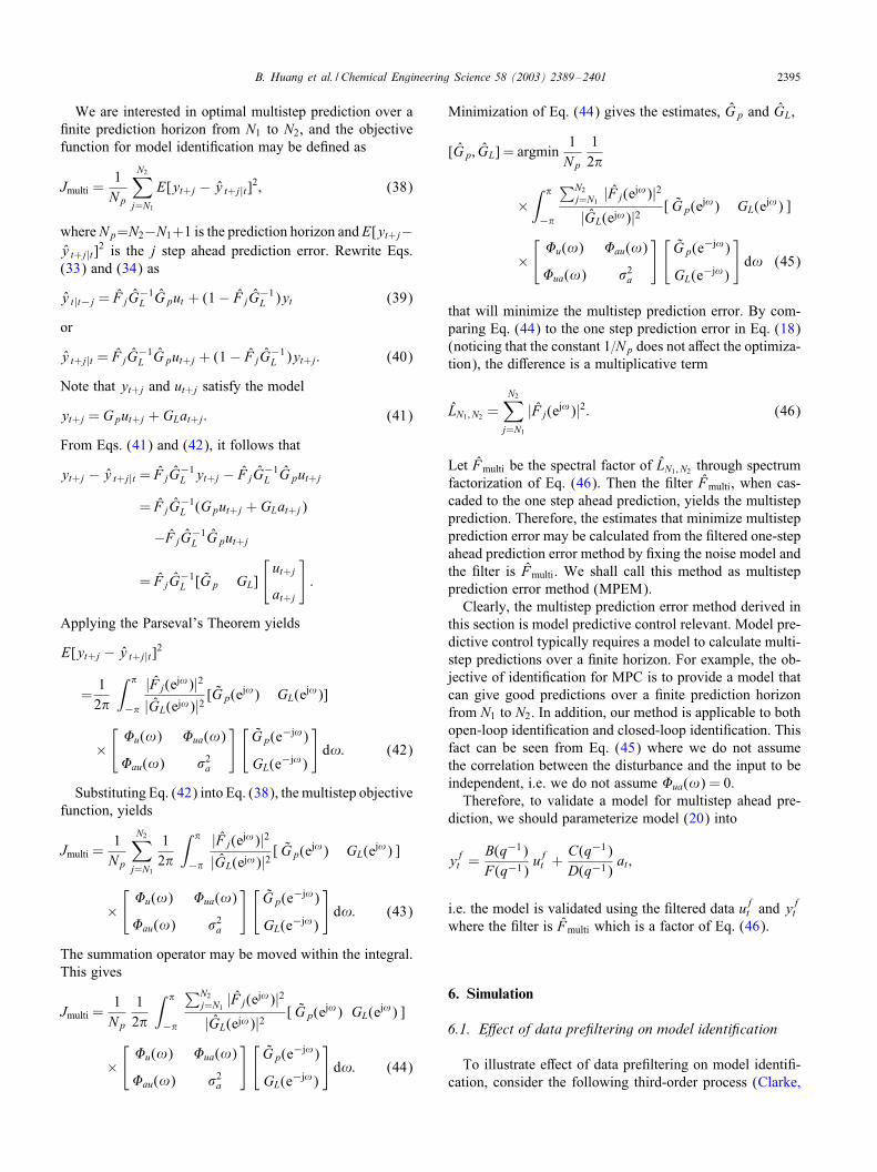
1.6Step response of the estimated models

true model PEM 2−step PEM 2 −step MPEM

Fig. 1. Step response of estimated models (using two-step KPEM andMPEM #lters).

Mohtadi, & TuJs, 1987):

G(q−1) =0:00768q−1 + 0:02123q−2 + 0:00357q−3

1− 1:9031q−1 + 1:1514q−2 − 0:2158q−3 (47)

with a random-walk disturbance.To investigate the eJect of data pre#ltering on the model

error, the following #rst-order model is used for identi#ca-tion:

Gp =b1q−1 + b2q−2

1− a1q−1:

In this section, we compare the models estimated by (1)PEM, (2) KPEM and (3) MPEM. As shown in previoussections, theoretically the PEM should give the best one-stepahead prediction, the KPEM should give the best k-stepahead prediction, and the MPEM should give the overallbest prediction over the entire prediction horizon.The step responses of the estimated models are shown in

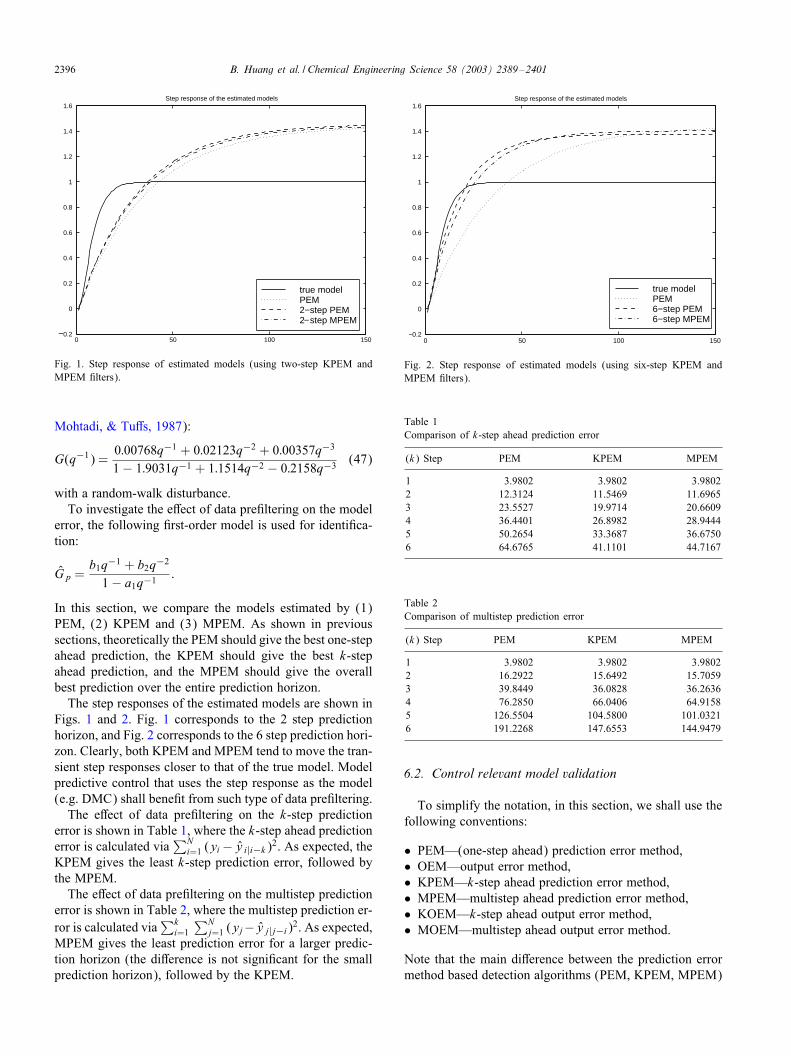
Figs. 1 and 2. Fig. 1 corresponds to the 2 step predictionhorizon, and Fig. 2 corresponds to the 6 step prediction hori-zon. Clearly, both KPEM and MPEM tend to move the tran-sient step responses closer to that of the true model. Modelpredictive control that uses the step response as the model(e.g. DMC) shall bene#t from such type of data pre#ltering.The eJect of data pre#ltering on the k-step prediction

error is shown in Table 1, where the k-step ahead predictionerror is calculated via

∑Ni=1 (yi − y i|i−k)2. As expected, the

KPEM gives the least k-step prediction error, followed bythe MPEM.The eJect of data pre#ltering on the multistep prediction

error is shown in Table 2, where the multistep prediction er-ror is calculated via

∑ki=1

∑Nj=1 (yj−y j|j−i)2. As expected,

MPEM gives the least prediction error for a larger predic-tion horizon (the diJerence is not signi#cant for the smallprediction horizon), followed by the KPEM.

0 50 100 150 −0.2

0

0.2

0.4

0.6

0.8

1

1.2

1.4

1.6Step response of the estimated models

true model PEM 6−step PEM 6−step MPEM

Fig. 2. Step response of estimated models (using six-step KPEM andMPEM #lters).

Table 1Comparison of k-step ahead prediction error

(k) Step PEM KPEM MPEM

1 3.9802 3.9802 3.98022 12.3124 11.5469 11.69653 23.5527 19.9714 20.66094 36.4401 26.8982 28.94445 50.2654 33.3687 36.67506 64.6765 41.1101 44.7167

Table 2Comparison of multistep prediction error

(k) Step PEM KPEM MPEM

1 3.9802 3.9802 3.98022 16.2922 15.6492 15.70593 39.8449 36.0828 36.26364 76.2850 66.0406 64.91585 126.5504 104.5800 101.03216 191.2268 147.6553 144.9479

6.2. Control relevant model validation

To simplify the notation, in this section, we shall use thefollowing conventions:

• PEM—(one-step ahead) prediction error method,• OEM—output error method,• KPEM—k-step ahead prediction error method,• MPEM—multistep ahead prediction error method,• KOEM—k-step ahead output error method,• MOEM—multistep ahead output error method.

Note that the main diJerence between the prediction errormethod based detection algorithms (PEM, KPEM, MPEM)


10-1 100 1010

0.1

0.2

0.3

0.4

0.5

0.6

0.7

0.8

0.9

1k-step ahead filter bode plot

Frequency (rad/sec)

Nor

mal

ized

Am

plitu

de R

atio

k = 5

k = 10

k = 15

k = 50

Fig. 3. Normalized amplitude bode plot of KPEM #lter (using 5, 10, 15and 50 step).

and output error method based detection algorithms (OEM,KOEM, MOEM) is whether the detection algorithm is sen-sitive to the changes of the disturbance transfer functions. Inaddition, the output error method based detection algorithmscannot handle the unstable random walk disturbances butthe prediction error method based algorithms can. The dis-turbance transfer function (model) is #xed in all validationalgorithms discussed in this section to the random walk:

GL =1

1− q−1: (48)

This is done as this form of the disturbance model is com-monly used in model predictive control. The KPEM andMPEM pre#lters are formed using this disturbance transferfunction (GL). The Bode plot of the normalized magnitudeof the KPEM #lter is given in Fig. 3. The #gure shows thedistribution of the magnitude plot over the frequency rangeof interest. It can be seen that the frequency distribution ofthe magnitude plot shifts towards the lower frequency bandas the prediction horizon is increased. With increased pre-diction horizon the frequency plot of the #lter approachesthat of a pure integrator. Due to this reason the detectionalgorithm with KPEM #ltering would be less sensitive tohigh-frequency model changes with an increased predictionhorizon.The normalized magnitude plot of the MPEM #lter is

given in Fig. 4. Here again it can be seen that the magnitudeplot shifts towards the lower frequency band as the predic-tion horizon is increased. Also the magnitude at the higherfrequencies decreases as the prediction horizon increases.In this simulation, we apply the proposed control rele-

vant detection algorithms to the process given by Eq. (47).As the output error method based validation algorithm can-not handle unstable disturbances, we simulate a disturbancewhich is very close to the random walk but stable, i.e. the

10-1 100 1010

0.1

0.2

0.3

0.4

0.5

0.6

0.7

0.8

0.9

1Multi step filter bode plot

Nor

mal

ized

Am

plitu

de R

atio

k = 5

k = 10

k = 15

k = 50

Frequency (rad/sec)

Fig. 4. Normalized amplitude bode plot of MPEM #lter (using 5; 10; 15and 50 step).

Fig. 5. Plot of �2 test using the KOEM-based detection algorithm.

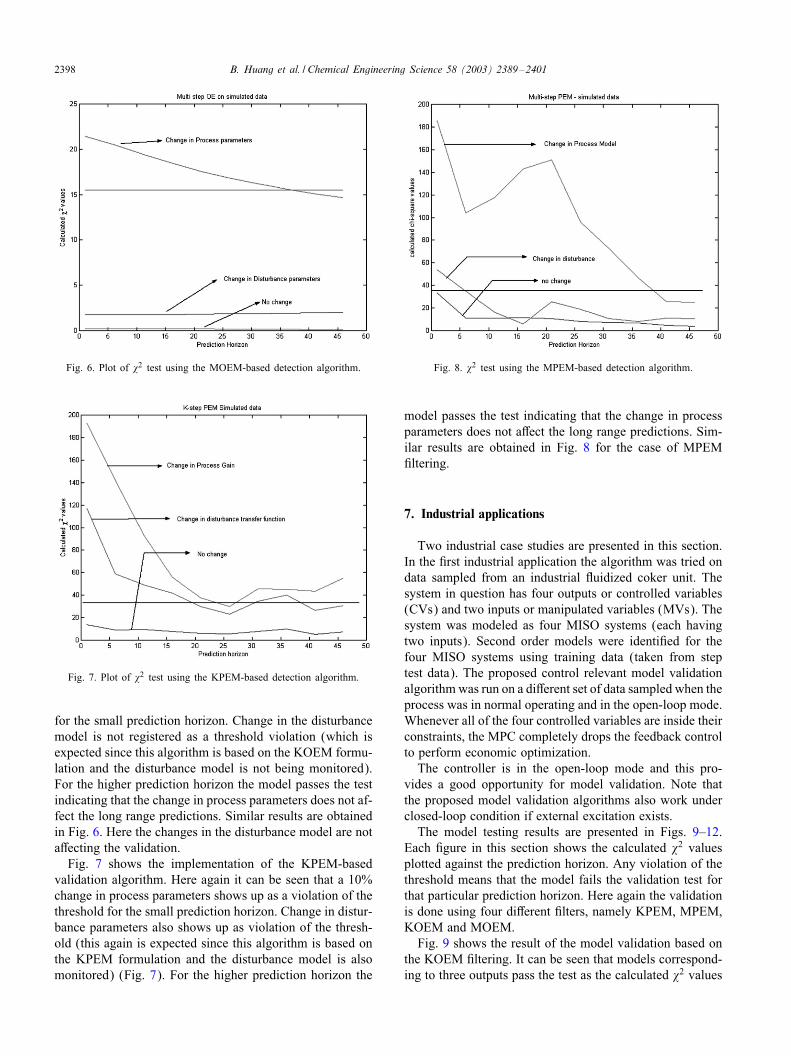
denominator of the disturbance transfer function used forthe simulation has a pole 0.99 (note that the disturbancemodel used for the detection algorithms is still the randomwalk). The input (ut) and noise term (at) are taken as zeromean random inputs with variance 0.3 and 0.1, respectively.DiJerent parameter changes are considered to test the eJec-tiveness of the validation algorithms. The results are shownin the following #gures where the calculated �2 values plotagainst the prediction horizon. A 10% change in parame-ters is taken for each case. Each #gure shows the result forthree scenarios—no change, change in process parametersand change in disturbance parameters. The threshold fromthe �2 table is also plotted in each #gure.Fig. 5 shows the implementation of the KOEM-based val-

idation algorithm. Here it can be seen that a 10 % change inprocess parameters shows up as a violation of the threshold


Fig. 6. Plot of �2 test using the MOEM-based detection algorithm.

Fig. 7. Plot of �2 test using the KPEM-based detection algorithm.

for the small prediction horizon. Change in the disturbancemodel is not registered as a threshold violation (which isexpected since this algorithm is based on the KOEM formu-lation and the disturbance model is not being monitored).For the higher prediction horizon the model passes the testindicating that the change in process parameters does not af-fect the long range predictions. Similar results are obtainedin Fig. 6. Here the changes in the disturbance model are notaJecting the validation.Fig. 7 shows the implementation of the KPEM-based

validation algorithm. Here again it can be seen that a 10%change in process parameters shows up as a violation of thethreshold for the small prediction horizon. Change in distur-bance parameters also shows up as violation of the thresh-old (this again is expected since this algorithm is based onthe KPEM formulation and the disturbance model is alsomonitored) (Fig. 7). For the higher prediction horizon the

Fig. 8. �2 test using the MPEM-based detection algorithm.

model passes the test indicating that the change in processparameters does not aJect the long range predictions. Sim-ilar results are obtained in Fig. 8 for the case of MPEM#ltering.

7. Industrial applications

Two industrial case studies are presented in this section.In the #rst industrial application the algorithm was tried ondata sampled from an industrial Yuidized coker unit. Thesystem in question has four outputs or controlled variables(CVs) and two inputs or manipulated variables (MVs). Thesystem was modeled as four MISO systems (each havingtwo inputs). Second order models were identi#ed for thefour MISO systems using training data (taken from steptest data). The proposed control relevant model validationalgorithmwas run on a diJerent set of data sampled when theprocess was in normal operating and in the open-loop mode.Whenever all of the four controlled variables are inside theirconstraints, the MPC completely drops the feedback controlto perform economic optimization.The controller is in the open-loop mode and this pro-

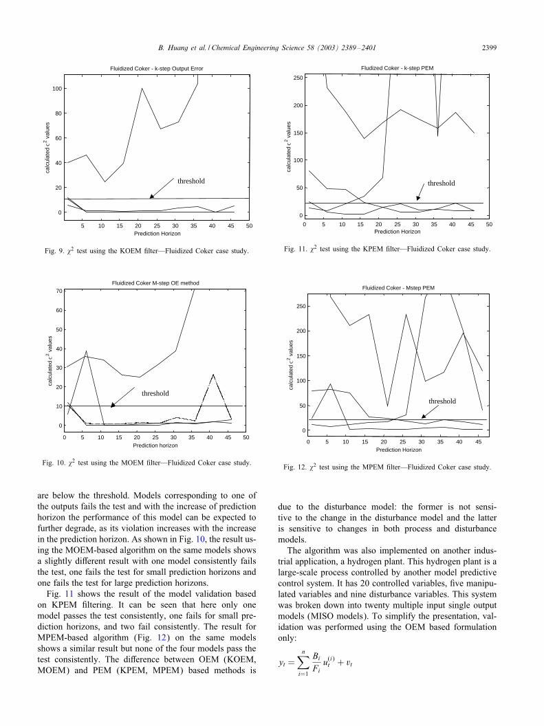
vides a good opportunity for model validation. Note thatthe proposed model validation algorithms also work underclosed-loop condition if external excitation exists.The model testing results are presented in Figs. 9–12.

Each #gure in this section shows the calculated �2 valuesplotted against the prediction horizon. Any violation of thethreshold means that the model fails the validation test forthat particular prediction horizon. Here again the validationis done using four diJerent #lters, namely KPEM, MPEM,KOEM and MOEM.Fig. 9 shows the result of the model validation based on

the KOEM #ltering. It can be seen that models correspond-ing to three outputs pass the test as the calculated �2 values


threshold

5 10 15 20 25 30 35 40 45 50

0

20

40

60

80

100

Fluidized Coker - k-step Output Error

Prediction Horizon

calc

ulat

ed c

2 val

ues

Fig. 9. �2 test using the KOEM #lter—Fluidized Coker case study.

0 5 10 15 20 25 30 35 40 45 50

0

10

20

30

40

50

60

70

Prediction horizon

calc

ulat

ed c

2 val

ues

Fluidized Coker M-step OE method

threshold

Fig. 10. �2 test using the MOEM #lter—Fluidized Coker case study.

are below the threshold. Models corresponding to one ofthe outputs fails the test and with the increase of predictionhorizon the performance of this model can be expected tofurther degrade, as its violation increases with the increasein the prediction horizon. As shown in Fig. 10, the result us-ing the MOEM-based algorithm on the same models showsa slightly diJerent result with one model consistently failsthe test, one fails the test for small prediction horizons andone fails the test for large prediction horizons.Fig. 11 shows the result of the model validation based

on KPEM #ltering. It can be seen that here only onemodel passes the test consistently, one fails for small pre-diction horizons, and two fail consistently. The result forMPEM-based algorithm (Fig. 12) on the same modelsshows a similar result but none of the four models pass thetest consistently. The diJerence between OEM (KOEM,MOEM) and PEM (KPEM, MPEM) based methods is

0 5 10 15 20 25 30 35 40 45 50

0

50

100

150

200

250

Fludized Coker - k-step PEM

Prediction Horizon

calc

ulat

ed c

2 val

ues

threshold

Fig. 11. �2 test using the KPEM #lter—Fluidized Coker case study.

0 5 10 15 20 25 30 35 40 45

0

50

100

150

200

250

Fluidized Coker - Mstep PEM

Prediction Horizon

calc

ulat

ed c

2 val

ues

threshold

Fig. 12. �2 test using the MPEM #lter—Fluidized Coker case study.

due to the disturbance model: the former is not sensi-tive to the change in the disturbance model and the latteris sensitive to changes in both process and disturbancemodels.The algorithm was also implemented on another indus-

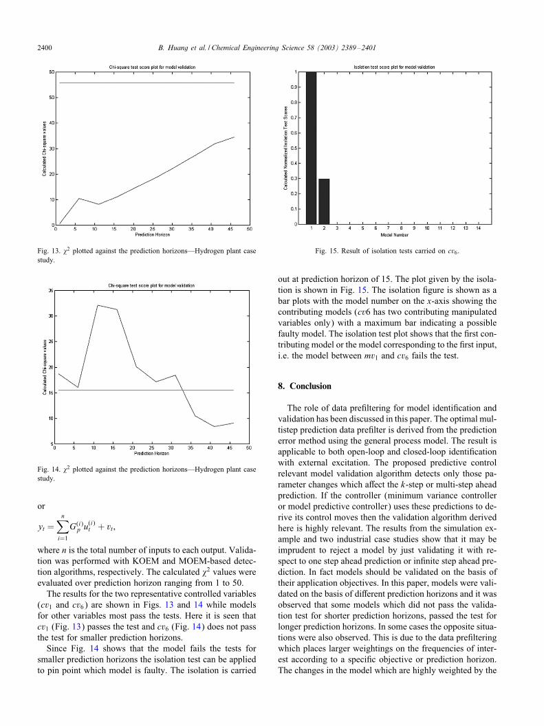
trial application, a hydrogen plant. This hydrogen plant is alarge-scale process controlled by another model predictivecontrol system. It has 20 controlled variables, #ve manipu-lated variables and nine disturbance variables. This systemwas broken down into twenty multiple input single outputmodels (MISO models). To simplify the presentation, val-idation was performed using the OEM based formulationonly:

yt =n∑

i=1

Bi

Fiu(i)t + vt


Fig. 13. �2 plotted against the prediction horizons—Hydrogen plant casestudy.

Fig. 14. �2 plotted against the prediction horizons—Hydrogen plant casestudy.

or

yt =n∑

i=1

G(i)p u(i)t + vt ;

where n is the total number of inputs to each output. Valida-tion was performed with KOEM and MOEM-based detec-tion algorithms, respectively. The calculated �2 values wereevaluated over prediction horizon ranging from 1 to 50.The results for the two representative controlled variables

(cv1 and cv6) are shown in Figs. 13 and 14 while modelsfor other variables most pass the tests. Here it is seen thatcv1 (Fig. 13) passes the test and cv6 (Fig. 14) does not passthe test for smaller prediction horizons.Since Fig. 14 shows that the model fails the tests for

smaller prediction horizons the isolation test can be appliedto pin point which model is faulty. The isolation is carried

Fig. 15. Result of isolation tests carried on cv6.

out at prediction horizon of 15. The plot given by the isola-tion is shown in Fig. 15. The isolation #gure is shown as abar plots with the model number on the x-axis showing thecontributing models (cv6 has two contributing manipulatedvariables only) with a maximum bar indicating a possiblefaulty model. The isolation test plot shows that the #rst con-tributing model or the model corresponding to the #rst input,i.e. the model between mv1 and cv6 fails the test.

8. Conclusion

The role of data pre#ltering for model identi#cation andvalidation has been discussed in this paper. The optimal mul-tistep prediction data pre#lter is derived from the predictionerror method using the general process model. The result isapplicable to both open-loop and closed-loop identi#cationwith external excitation. The proposed predictive controlrelevant model validation algorithm detects only those pa-rameter changes which aJect the k-step or multi-step aheadprediction. If the controller (minimum variance controlleror model predictive controller) uses these predictions to de-rive its control moves then the validation algorithm derivedhere is highly relevant. The results from the simulation ex-ample and two industrial case studies show that it may beimprudent to reject a model by just validating it with re-spect to one step ahead prediction or in#nite step ahead pre-diction. In fact models should be validated on the basis oftheir application objectives. In this paper, models were vali-dated on the basis of diJerent prediction horizons and it wasobserved that some models which did not pass the valida-tion test for shorter prediction horizons, passed the test forlonger prediction horizons. In some cases the opposite situa-tions were also observed. This is due to the data pre#lteringwhich places larger weightings on the frequencies of inter-est according to a speci#c objective or prediction horizon.The changes in the model which are highly weighted by the


data pre#lter will be easily detected. The changes in otherfrequencies (other than those highly weighted by the #lter)will be in fact suppressed.

References

Basseville, M. (1998). On-board component fault detection and isolationusing the statistical local approach. Automatica, 34(11), 1391–1415.

Benveniste, A., Basseville, M., & Moustakides, G. V. (1987). Theasymptotic local approach to change detection and model validation.IEEE Transactions on Automatic Control, 32(7), 583–592.

Bitmead, R. R., Gevers, M., & Wertz, V. (1990). Adaptive optimalcontrol. Englewood CliJs, NJ: Prentice-Hall.

Clarke, D. W., Mohtadi, C., & TuJs, P. S. (1987). Generalized predictivecontrol—Part 1 and 2. Automatica, 23(2), 137–160.

Cooley, B., & Lee, J. H. (1998). Integrated identi#cation and robustcontrol. Journal of Process Control, 8, 431–440.

Huang, B. (2000). Model validation in the presence of time-variantdisturbance dynamics. Chemical Engineering Science, 55, 4583–4595.

Huang, B., & Tamayo, E. C. (2000). Model validation for industrial modelpredictive control systems. Chemical Engineering Science, 55(12),2315–2327.

Larimore, W.E. (1990). Canonical variate analysis in identi#cation,#ltering and adaptive control. Proceedings of the 29th IEEEConference on Decision and Control, Vol. 29 (594–604).

Ljung, L. (1999). System identi8cation (2nd ed.). Englewood CliJs, NJ:Prentice-Hall.

Ljung, L., & Guo, L. (1997). The role of model validation for assessingthe size of the unmodeled dynamics. IEEE Transactions on AutomaticControl, 42(9), 1230–1239.

Rivera, D. E., Pollard, J. F., & Garcia, C. E. (1992). Control-relevantpre#ltering: A systematic design approach and case study. IEEETransactions on Automatic Control, 37(7), 964–974.

Shook, D. S., Mohtadi, C., & Shah, S. L. (1992). A control-relevantidenti#cation strategy for gpc. IEEE Transactions on AutomaticControl, 37(7), 975–980.

Soderstrom, T., & Stoica, P. (1989). System identi8cation. EnglewoodCliJs, NJ, UK: Prentice-Hall International.

Sternad, M., & Soderstrom, T. (1988). Lqg-optimal feedforwardregulators. Automatica, 24(4), 557–561.

Van den Hof, P. M. J., & Schrama, R. J. P. (1995). Identi#cation andcontrol—closed-loop issues. Automatica, 31(12), 1751–1770.

Van Overschee, P., & De Moor, B. (1996). Subspace identi8cationfor linear systems: Theory implementation applications. Dordrecht:Kluwer Academic Publishers.

Verhaegen, M. (1994). Identi#cation of the deterministic part of mimostate space models given in innovations form from input–output data.Automatica, 30(1), 61–74.

Zhang, Q., Basseville, M., & Benveniste, A. (1994). Early warning ofslight changes in systems. Automatica, 30(1), 95–113.

Zhang, Q., Basseville, M., & Benveniste, A. (1998). Fault detection andisolation in nonlinear dynamic systems: A combined input–output andlocal approach. Automatica, 34(11), 1359–1373.

Zang, Z., Bitmead, R. R., & Gevers, M. (1995). Iterative weightedleast-squares identi#cation and weighted lqg control design.Automatica, 31(11), 1577–1594.

Model predictive control relevant identification and validation

Documents

Transcript of Model predictive control relevant identification and validation