
Model Predictive Control of a Grid-Connected Converter With ...
111
Model Predictive Control of a Grid-Connected Converter With LCL-Filter by Joanie Michellene Claudette Geldenhuys Thesis presented in partial fulfilment of the requirements for the degree of Master of Science in Electrical and Electronic Engineering in the Faculty of Engineering at Stellenbosch University Department of Electrical and Electronic Engineering, University of Stellenbosch, Private Bag X1, Matieland 7602, South Africa. Supervisors: Prof. H. du T. Mouton and Dr. A. Rix March 2018
-
Upload
khangminh22 -
Category
Documents
-
view
3 -
download
0
Transcript of Model Predictive Control of a Grid-Connected Converter With ...

Model Predictive Control of aGrid-Connected Converter With LCL-Filter
by
Joanie Michellene Claudette Geldenhuys
Thesis presented in partial fulfilment of the requirements for the degree of Master of Science in Electrical and Electronic Engineering in the Faculty of Engineering at Stellenbosch
University
Department of Electrical and Electronic Engineering, University of Stellenbosch,
Private Bag X1, Matieland 7602, South Africa.
Supervisors:
Prof. H. du T. Mouton and Dr. A. Rix
March 2018

Declaration
By submitting this thesis electronically, I declare that the entirety of thework contained therein is my own, original work, that I am the sole authorthereof (save to the extent explicitly otherwise stated), that reproduction andpublication thereof by Stellenbosch University will not infringe any third partyrights and that I have not previously in its entirety or in part submitted it forobtaining any qualification.
2017/12/01Date: . . . . . . . . . . . . . . . . . . . . . . . . . . . . . . .
Copyright © 2018 Stellenbosch UniversityAll rights reserved.
i
Stellenbosch University https://scholar.sun.ac.za

Abstract
Model Predictive Control of a Grid-Connected ConverterWith LCL-FilterJ.M.C. Geldenhuys
Department of Electrical and Electronic Engineering,University of Stellenbosch,
Private Bag X1, Matieland 7602, South Africa.
Thesis: MScEng (E&E)March 2018
Improved efficiency of power conversion is high priority when it comes torenewable energy applications. Model predictive control (MPC) can be usedto optimise the switching pattern applied in the converter to reduce switchinglosses. During this research the suitability of a direct MPC strategy with longhorisons is evaluated for current control of a three-phase two-level grid-tiedconverter with LCL-filter.
A cost function was formulated to include two weighted control objectives,namely reducing the reference tracking error and switching frequency. Thegrid voltage was incorporated into the state-space model as an additionalinput vector. Therefore the optimisation approach, used to transform thecost-function minimisation problem towards the integer least-squares (ILS)problem, had to be reworked to consider this additional element, herebyextending on previous work done on the integer quadratic programmingformulation for long horisons. A sphere decoding algorithm was incorporatedto reduce the computational burden.
The current controller shows fast transient response and good referencetracking of the fundamental 50 Hz component. The developed strategycomplies to the grid-side current harmonic limits set out in the South Africangrid code at high switching frequencies, but is unable to comply to the evenand high-order harmonic limits at low switching frequencies.
ii
Stellenbosch University https://scholar.sun.ac.za

Uittreksel
Model Voorspellende Beheer van ’n Netwerk-GekoppeldeOmsetter met ’n LCL-Filter
(“Model Predictive Control of a Grid Connected Converter With LCL-Filter”)
J.M.C. GeldenhuysDepartement Elektriese en Elektroniese Ingenieurswese,
Universiteit van Stellenbosch,Privaatsak X1, Matieland 7602, Suid Afrika.
Tesis: MScIng (E&E)Maart 2018
Verbeterde doeltreffendheid van kragomsetting is ’n hoë prioriteit wat betrefhernubare energie toepassings. Model voorspellende beheer (MVB) kangebruik word om die skakelpatroon wat in die omsetter toegepas is te optimeerom skakelverliese te verminder. Gedurende hierdie navorsing is die geskiktheidvan direkte MVB met lang horisonne ge-evalueer vir die beheer van ’n drie-fase,twee-vlak, netwerkgekoppelde omsetter met ’n LCL-filter.
’n Kostefunksie is geformuleer om twee beheermikpunte, naamlikdie vermindering van die stroomvolgfout en skakelfrekwensie in tesluit. Die netwerkspanning is by die toestandsruimte model as ’nbykomende intreevektor inkorporeer. Hierdie bykomende element hetgemaak dat die optimeringsbenadering wat gebruik is om die kostefunksieminimeringsprobleem tot die kleinste vierkant probleem te transformer,gewysig moes word. Dit is ’n voortsetting van vorige werk oor heeltalligekwadratiese programmeringsformulering vir lang horison toepassings. ’nAlgoritme vir ’n sfeer dekodeerder is geïmplementeer om die berekeningslaste verminder.
Die stroombeheerder wys vinnige oorgang en bied akkurate stoomvolgingvan die 50Hz fundamentele frekwensie komponent. Die ontwikkelde strategievoldoen teen hoë skakelfrekwensies aan netwerkstroom harmoniekbeperkingssoos in die Suid-Afrikaanse netwerkkode uiteengesit, maar kan nie teen laefrekwensies voldoen aan die ewe en hoë orde harmoniekbeperkinge nie.
iii
Stellenbosch University https://scholar.sun.ac.za

List of Publications
Geldenhuys, J., Mouton, H.d.T. and Rix, A.: Current control of a grid-tiedinverter with LCL-Filter through model predictive control. : Southern AfricanUniversities Power Engineering Conference (SAUPEC). Vereeniging, SouthAfrica, 2016.
Geldenhuys, J., Mouton, H.d.T., Rix, A. and Geyer, T.: Model predictivecontrol of a grid connected converter with LCL-Filter. : Proceedings ofthe 17th IEEE Workshop on Control and Modeling for Power Electronics(COMPEL 2016). Trondheim, Norway, 2016.
iv
Stellenbosch University https://scholar.sun.ac.za

Acknowledgements
To my Creator, thank you for the opportunity and ability You have given me,and how You have always strengthened me during my hardest times. I giveYou all the glory.
My sincere gratitude to my project supervisors and mentors, ProfessorMouton and Dr. Rix. Thank you for your patience, understanding, guidanceand the sharing of your knowledge during this research.
Scatec Solar, thank you for your generous support in providing me with ascholarship. I would not have had the opportunity to do a master’s degreewithout your support.
Heinrich, your amazing drive and perseverance inspires me to prevailand to see beyond that which seems impossible. Thank you for never allowingme to doubt myself.
My parents, Willem and Felicity Engelbrecht, you have always given ahundred-and-ten per cent of yourselves to your children. I realise now howmuch you have sacrificed so that I can grow and excel. Your dedicated prayeralso means a lot to me.
My parents-in-law, Jacques and Lucresia Geldenhuys, thank you for thesupport you have given me and your son, Heinrich.
Thank you to all my family and friends who kept us in their prayersand provided support and understanding.
v
Stellenbosch University https://scholar.sun.ac.za

Dedication
This thesis is dedicated to my husband Heinrich, you have changed my life inradical and exciting ways. Thank you for being an inspirational life partner.
vi
Stellenbosch University https://scholar.sun.ac.za

Contents
Declaration i
Abstract ii
Uittreksel iii
List of Publications iv
Acknowledgements v
Dedication vi
Contents vii
List of Figures ix
List of Tables xii
Nomenclature xiii
1 Introduction 11.1 Background to the research problem . . . . . . . . . . . . . . . . 11.2 Renewable energy . . . . . . . . . . . . . . . . . . . . . . . . . . 31.3 Research statement . . . . . . . . . . . . . . . . . . . . . . . . . 61.4 Research objectives . . . . . . . . . . . . . . . . . . . . . . . . . 61.5 Brief overview of the research . . . . . . . . . . . . . . . . . . . 6
2 Background and Literature Review 92.1 Power converters . . . . . . . . . . . . . . . . . . . . . . . . . . 92.2 Types of control methods . . . . . . . . . . . . . . . . . . . . . 102.3 Suitability of predictive control schemes . . . . . . . . . . . . . . 122.4 Model predictive control . . . . . . . . . . . . . . . . . . . . . . 142.5 Basic principles of model predictive control . . . . . . . . . . . 162.6 Existing research . . . . . . . . . . . . . . . . . . . . . . . . . . 222.7 Summary . . . . . . . . . . . . . . . . . . . . . . . . . . . . . . 27
vii
Stellenbosch University https://scholar.sun.ac.za

CONTENTS viii
3 System and Controller Design 293.1 Introduction . . . . . . . . . . . . . . . . . . . . . . . . . . . . . 293.2 System Topology . . . . . . . . . . . . . . . . . . . . . . . . . . 293.3 Constraints . . . . . . . . . . . . . . . . . . . . . . . . . . . . . 303.4 Reference frames . . . . . . . . . . . . . . . . . . . . . . . . . . 303.5 State-space model . . . . . . . . . . . . . . . . . . . . . . . . . . 313.6 Cost function . . . . . . . . . . . . . . . . . . . . . . . . . . . . 333.7 Optimisation approach . . . . . . . . . . . . . . . . . . . . . . . 353.8 Sphere Decoding . . . . . . . . . . . . . . . . . . . . . . . . . . 423.9 Summary . . . . . . . . . . . . . . . . . . . . . . . . . . . . . . 44
4 Implementation and Results 464.1 Introduction . . . . . . . . . . . . . . . . . . . . . . . . . . . . . 464.2 Simulation design . . . . . . . . . . . . . . . . . . . . . . . . . . 464.3 Spectral analysis of MPC . . . . . . . . . . . . . . . . . . . . . . 564.4 Performance evaluation and comparison . . . . . . . . . . . . . 644.5 Summary . . . . . . . . . . . . . . . . . . . . . . . . . . . . . . 75
5 Discussion and Conclusion 775.1 Summary of the research . . . . . . . . . . . . . . . . . . . . . . 775.2 Main findings . . . . . . . . . . . . . . . . . . . . . . . . . . . . 805.3 Suggestions for future research . . . . . . . . . . . . . . . . . . . 825.4 Conclusion . . . . . . . . . . . . . . . . . . . . . . . . . . . . . . 82
Appendices 84
A Additional Theory 85A.1 Bessel function . . . . . . . . . . . . . . . . . . . . . . . . . . . 85A.2 Grid code . . . . . . . . . . . . . . . . . . . . . . . . . . . . . . 86
List of References 87
Stellenbosch University https://scholar.sun.ac.za

List of Figures
1.1 Total electricity produced globally, analysed according to source.Produced from data in [1; 2; 3]. . . . . . . . . . . . . . . . . . . . 1
1.2 Comparison of LCOE costs for PV and coal-generated electricityfrom actual and predicted data. Reproduced from [4; 5]. . . . . . . 3
1.3 Different types of renewable energy. Reproduced from [6; 7]. . . . . 41.4 General configuration to connect a photovoltaic power plant to the
grid [8]. . . . . . . . . . . . . . . . . . . . . . . . . . . . . . . . . . 51.5 Brief overview of the thesis chapters. . . . . . . . . . . . . . . . . . 7
2.1 System diagram for a renewable energy power converterapplication. Amended from [9]. . . . . . . . . . . . . . . . . . . . . 10
2.2 A classification of converter control methods for power convertersand drives. Amended from [10]. . . . . . . . . . . . . . . . . . . . . 11
2.3 Characteristics of power converters, the nature of control platformspresently available and their relation to predictive controlapproaches. Amended from [10]. . . . . . . . . . . . . . . . . . . . . 13
2.4 Classification of predictive control methods. Amended from [11]. . 142.5 Example of a physical model of the system. A single-phase,
two-level grid-tied converter with LCL-filter is used per illustration.From such a model a mathematical model is derived. . . . . . . . . 16
2.6 Diagram of how the MPC control scheme functions. Amendedfrom [10]. . . . . . . . . . . . . . . . . . . . . . . . . . . . . . . . . 17
2.7 Mapping of all the possible switching actions and their resultingcurrent trajectories. Amended from [12]. . . . . . . . . . . . . . . . 18
2.8 Exhaustive solution search tree of a three-level converter setup overa horison length of three steps into the future. Amended from [13]. 19
2.9 Solution space of a three-level converter, evaluated over a horisonof N = 3 time steps, containing the 27 solution points of whichtwo fall within the search sphere centred around the unconstrainedsolution. . . . . . . . . . . . . . . . . . . . . . . . . . . . . . . . . . 20
2.10 Pruning of the search tree for a three-level converter setup by meansof the sphere decoding algorithm over a horison length of three timesteps into the future [13]. . . . . . . . . . . . . . . . . . . . . . . . . 21
2.11 System topology used by [14]. Amended from [14]. . . . . . . . . . 24
ix
Stellenbosch University https://scholar.sun.ac.za

LIST OF FIGURES x
2.12 Frequency response of the digital filters W1,W2 and Wr. Amendedfrom [14]. . . . . . . . . . . . . . . . . . . . . . . . . . . . . . . . . 26
2.13 Spectrum of the converter-side current i1 compared to its filter.Amended from [14]. . . . . . . . . . . . . . . . . . . . . . . . . . . . 26
2.14 Spectrum of the grid-side current i2 compared to its filter.Amended from [14]. . . . . . . . . . . . . . . . . . . . . . . . . . . . 27
2.15 Brief overview of the thesis chapters. . . . . . . . . . . . . . . . . . 28
3.1 Three-phase grid-connected converter with LCL-filter. . . . . . . . . 303.2 Per-phase model of the LCL-filter. . . . . . . . . . . . . . . . . . . 313.3 Per-phase model of the LCL-filter. . . . . . . . . . . . . . . . . . . 343.4 Reference tracking and evolution of the output y as a function of
the input switching sequence for a horison of N = 2. Amendedfrom [12]. . . . . . . . . . . . . . . . . . . . . . . . . . . . . . . . . 36
3.5 Visualisation of the optimisation problem for a three-phase systemwith a horison ofN = 1 in an orthogonal coordinate system (dashedblue line) and how it compares with the transformed problem (solidgreen line). . . . . . . . . . . . . . . . . . . . . . . . . . . . . . . . 41
3.6 Top view of Figure 3.5 showing the ab-plane to gain perspective onthe sphere and the points which lie closest to its centre. . . . . . . . 44
3.7 Brief overview of the thesis chapters. . . . . . . . . . . . . . . . . . 45
4.1 Main function flow diagram of the direct MPC simulation script. . . 474.2 An example of how adjustment of the weighting factor can influence
the current-tracking error for a single-phase controller with a longhorison of N = 12. . . . . . . . . . . . . . . . . . . . . . . . . . . . 49
4.3 An example of how switching frequency changes with theadjustment of the weighting factor for a single-phase controller witha long horison of N = 12. . . . . . . . . . . . . . . . . . . . . . . . 50
4.4 FLOPS executed during an exhaustive search, and during anoptimised search using sphere decoding. . . . . . . . . . . . . . . . 51
4.5 Resulting grid-side current and reference for a controller thatdisregards the grid-voltage in the optimisation approach. . . . . . 52
4.6 Steady-state three-phase output currents and references using along horison of N = 12. . . . . . . . . . . . . . . . . . . . . . . . . 53
4.7 Inductor currents and references in the a-phase during steady-stateoperation with a long horison of N = 12. . . . . . . . . . . . . . . . 53
4.8 Capacitor voltage and its reference in the a-phase duringsteady-state operation with a long horison of N = 12. . . . . . . . . 54
4.9 Response of inductor currents to a step in the reference amplitudeusing a short horison of N = 1. . . . . . . . . . . . . . . . . . . . . 55
4.10 Response of inductor currents to a step in the reference amplitudeusing a long horison of N = 12. . . . . . . . . . . . . . . . . . . . . 55
Stellenbosch University https://scholar.sun.ac.za

LIST OF FIGURES xi
4.11 Response of inductor currents to an unanticipated step in thereference amplitude using a long horison of N = 12. . . . . . . . . . 56
4.12 Output-current spectrum of the a-phase. . . . . . . . . . . . . . . . 574.13 Output-current spectrum of the a-phase with discrete harmonics. . 574.14 Converter-current spectrum of the a-phase with discrete harmonics. 584.15 Per-phase model of the LCL-filter. . . . . . . . . . . . . . . . . . . 594.16 Output current spectrum of the a-phase (PWM). . . . . . . . . . . 614.17 Triangular carrier, space-vector modulation signal and sinusoidal
waveform generated to determine the switching pulse widths. . . . . 624.18 Space-vector modulated switching pulses. . . . . . . . . . . . . . . . 624.19 Output current spectrum obtained from space vector modulation. . 644.20 Results for the MPC short-horison (N = 1) case at fsw = 1.2 kHz. . 664.21 Results for the MPC long-horison (N = 12) case at fsw = 1.2 kHz. . 674.22 Results for the PWM case at fsw = 1.2 kHz. . . . . . . . . . . . . . 684.23 Results for the SVM case at fsw = 1.2 kHz. . . . . . . . . . . . . . 694.24 Results for the MPC short-horison (N = 1) case at fsw = 10.3 kHz. 714.25 Results for the MPC long-horison (N = 12) case at fsw = 10.3 kHz. 724.26 Results for the PWM case at fsw = 10.3 kHz. . . . . . . . . . . . . 734.27 Results for the SVM case at fsw = 10.3 kHz. . . . . . . . . . . . . . 744.28 Brief overview of the thesis chapters. . . . . . . . . . . . . . . . . . 76
A.1 Output of a first order Bessel function. [15]. . . . . . . . . . . . . . 85
Stellenbosch University https://scholar.sun.ac.za

List of Tables
4.1 System parameters . . . . . . . . . . . . . . . . . . . . . . . . . . . 484.2 Summary of the simulation results . . . . . . . . . . . . . . . . . . 70
A.1 Current distortion limits according to harmonics [16]. . . . . . . . . 86
xii
Stellenbosch University https://scholar.sun.ac.za

Nomenclature
Constantsπ = 3.14159
j =√
(−1)
VariablesC Capacitance . . . . . . . . . . . . . . . . . . . . . [F ]f Frequency . . . . . . . . . . . . . . . . . . . . . . [Hz ]fs Sampling frequency . . . . . . . . . . . . . . . . [Hz ]fsw Switching frequency . . . . . . . . . . . . . . . . [Hz ]i Instantaneous current . . . . . . . . . . . . . . . [A ]J Cost . . . . . . . . . . . . . . . . . . . . . . . . . [ ]k Discrete time index . . . . . . . . . . . . . . . . [ ]L Inductance . . . . . . . . . . . . . . . . . . . . . [H ]ma Amplitude modulation index . . . . . . . . . . [ ]N Horison length . . . . . . . . . . . . . . . . . . . [ ]R Resistance . . . . . . . . . . . . . . . . . . . . . . [Ω ]t Time . . . . . . . . . . . . . . . . . . . . . . . . . [ s ]Ts Sampling period . . . . . . . . . . . . . . . . . . [ s ]u Switch state . . . . . . . . . . . . . . . . . . . . . [ ]v Instantaneous voltage . . . . . . . . . . . . . . . [V ]Z Impeadance . . . . . . . . . . . . . . . . . . . . . [Ω ]λ Weighting factor . . . . . . . . . . . . . . . . . . [ ]φ Modulation angle . . . . . . . . . . . . . . . . . [ deg ]ρ Radius . . . . . . . . . . . . . . . . . . . . . . . . [ ]ω Angular velocity . . . . . . . . . . . . . . . . . . [ rad/s ]
Vectors and MatricesH Lattice-generator (transformation) matrixu Switch state (three-phase)
xiii
Stellenbosch University https://scholar.sun.ac.za

NOMENCLATURE xiv
vg Grid voltage vectorx State vectory Output vector (three-phase)U Switching sequenceY Predicted output sequenceY ∗ Reference output sequenceξ XiΓ GammaΘ ThetaΥ UpsilonΨ Psi
Subscriptsa a-phaseabc abc reference frameb b-phasec c-phaseC Capacitore Errorg Gridini Initialopt Optimals Samplingsw Switchingunc Unconstrainedα α-component in the αβ reference frameαβ αβ reference frameβ β-component in the αβ reference frame
AbbreviationsA AmpereAC Alternating currentAD Active dampingdB DecibelDC Direct currentDNI Direct nominal irradiationDPC Direct power control
Stellenbosch University https://scholar.sun.ac.za

NOMENCLATURE xv
DTC Direct torque controlEMC Electromagnetic compatibilityF FaradFCS Finite-control setFLOPS Floating point operationsFOC Field orientated controlGC Grid codeGPC Generalised predictive controlH HenryHz HertzIEC International Electronic CommissionILS Integer least-squaresIM Induction machineIRP Integrated Resource PlanLCL Inductor-capacitor-inductor configurationLCOE Levelised cost of electricityk KiloKVL Kirchoff’s voltage lawMPC Model predictive controlMPCC Model predictive current controlMPDCC Model predictive direct current controlMPDTC Model predictive direct torque controlMV Medium voltageMW MegawattMVB Model voorspellende beheerNERSA National energy regulator of South AfricaNPC Neutral-point-clampedPI Proportional-integralPV PhotovoltaicPWM Pulse width modulationREI4P Renewable Energy Independent Power Producer
Procurement Programme (REIPPPP)s SecondsSA South AfricaSTFT Short-time Fourier transformSVM Space vector modulationTHD Total harmonic distortion
Stellenbosch University https://scholar.sun.ac.za

NOMENCLATURE xvi
TWh Terawatt hourVR Virtual resistorVOC Voltage-orientated controlVSC Voltage-source converterV Volts
Stellenbosch University https://scholar.sun.ac.za

Chapter 1
Introduction
1.1 Background to the research problemEnergy is regarded as an important building block of society and is required forthe creation of goods from natural resources [17]. Fossil fuels such as oil, coaland gas are still predominantly used for electricity production, but renewableenergy sources have since the 1970s slowly gained importance [17]. Globalenergy demand and access of renewable energy sources to the electricity gridare rapidly growing in proportion [18], as can be seen in Figure 1.1. Despite anincrease in energy efficiencies over time, an immense increase in global energydemand is predicted from now until 2040, especially in developing countries[19; 20; 21].
Renewable energy is currently projected as the fastest-growing energy
Figure 1.1: Total electricity produced globally, analysed according to source.Produced from data in [1; 2; 3].
1
Stellenbosch University https://scholar.sun.ac.za

CHAPTER 1. INTRODUCTION 2
source with its global consumption predicted to increase by an average of 2.6%per year until 2040 [19]. Integrating renewable energy sources into the gridcan bring many environmental and economic benefits [22]. Key challengesentail managing variability of supply from renewable energy sources withregards to integration with the power grid, and remaining competitive withtraditional power generation [21]. Renewable energy sources have receivedgrowing interest as a valuable means for nations to reduce their carbonemission [23; 24; 25].
Political commitments were made at the United Nations conference onclimate change where nations agreed to promote the universal access torenewable energy and its deployment [26; 24; 21]. The South African nationalobjective is to have 30% clean energy by 2025 [27].
South Africa’s solar potential is among the highest in the world, yetcoal-generated electricity still dominates [28]. Coal, linked to high carbonemissions, supplies 93% of South-African energy [29], and can be dated to theearly 1880s when the Kimberley diamond fields were supplied with coal fromVereeniging [30]. This is high compared to the world average which is around40% [31]. Coal has for many years been the preferred source of electricitygeneration in South Africa due to abundant local coal reserves, relative costeffectiveness and reliability [30].
In the SA White Paper on Energy Policy published in 1998 it is advocatedthat South Africa should improve on its energy efficiency [32] in order forthe country to maintain its economic competitiveness [33] since worldwideeconomic development is influenced by the production of electricity [34].The South African government has realised the importance of creating asustainable energy mix by investing in renewable energy resources. This ledto the White Paper on Renewable Energy in 2003 in which renewable energyinvestment through well-structured tariffs and creating public awareness onthe use of renewable energy and energy efficiency is promoted [35]. TheIntegrated Resource Plan (IRP) followed in 2010 and the Renewable EnergyIndependent Power Producer Procurement Programme (REI4P) in 2014 todrive the installation of renewable electricity generation capacity until 2030.Initially the REI4P was seen as an expensive option used to counter criticismof the country’s coal dependance and high carbon footprint [4]. However,this later changed due to the increasing competitiveness of the REI4P biddingprocess, the escalating costs of coal-based electricity generation and the rapidlydecreasing costs for wind and photovoltaic power [4]. This trend is supportedby the comparison of the levelised cost of electricity (LCOE) for PV andcoal-generated electricity in Figure 1.2. Renewable energy is finally gatheringmomentum in South Africa [4]. In 2014 South Africa was the country with thelargest renewable energy asset growth and made the eighth largest investmentsin renewable energy [36].
Stellenbosch University https://scholar.sun.ac.za

CHAPTER 1. INTRODUCTION 3
Figure 1.2: Comparison of LCOE costs for PV and coal-generated electricityfrom actual and predicted data. Reproduced from [4; 5].
1.2 Renewable energySources of electricity generation such as nuclear and fossil fuels (oil, coaland natural gas) are unsustainable as the replenish rate of these resourcescannot indefinitely support continued electricity generation in the future[37; 38; 39; 40]. The process of generating electricity from these non-renewablesources also leads to damage of the environment [37]. A more sustainableoption is renewable energy as it holds the potential to be economicallyviable, environmentally friendly and to bring socio-economic benefits such asemployment creation [4; 41], which align with the three pillars of sustainabledevelopment (economic, environmental and social sustainability).
Renewable energy sources are constantly replenished by the environmentwith the energy obtained from the sun either directly (for examplephoto-electric, photo-chemical and thermal), or indirectly (bioenergy, hydroand wind), as well as from other natural phenomena (such as tidal andgeothermal energy) [42]. In Figure 1.3 the different types of renewable energyare listed [6; 7].
In South Africa renewable energy can be traced back to 100 years ago whenfarmers used windmills for pumping water or grinding grain [43; 44]. Howeverit is only from the 1970s that the first attempts were made as to developrenewable energy technologies on a commercially viable scale [43].
These renewable energy technologies have evolved and passed the stageof trying to catch up with fossil fuel technologies and are now ratherpositioned to have equivalent or surpassing performance [43]. Traditional
Stellenbosch University https://scholar.sun.ac.za

CHAPTER 1. INTRODUCTION 4
Figure 1.3: Different types of renewable energy. Reproduced from [6; 7].
fossil fuel technologies have undergone a process of refinement spanningover more than a century, requiring trillions of dollars in subsidies, researchand development [43]. Currently these traditional technologies require largeinvestment to produce marginal improvement, while many renewable energytechnologies are in an innovation phase where small investments are bringingabout large performance gains and cost reductions [43].
One of the technologies that greatly influence the performance of renewableenergy systems is power electronics [42; 45]. Wind energy systems usepower electronic converters to regulate the variable input power and maximiseelectrical energy converted from the wind energy [42]. Inverters are used inphotovoltaic (PV) systems to effectively convert the DC voltage to AC forconnection to the electrical grid or other AC applications [42]. A typicalgrid-connected setup for a PV system is presented in Figure 1.4.
1.2.1 Research focus
Power electronics entail the control and conversion of electricity by means ofapplying a certain sequence of operation to semiconductor switches [42]. Inrenewable energy technologies efficiency is a priority especially in high powersystems. One measure that can reduce losses in the system is to minimiseswitching losses by switching the semiconductor devices at lower frequencies.This however compromises the quality of the current injected into the grid.Model predictive control (MPC) can be used to perform current control byeffectively managing the trade-off between switching frequency and currentreference tracking. It is a control method that has received increasing attentionwithin power electronics and entails online optimisation of a cost function thatencompasses the control objectives. Finite control set (FCS) model predictivecontrol, alternatively known as direct MPC, directly changes the switch statesof the semiconductor switches, which is therefore seen as the manipulated
Stellenbosch University https://scholar.sun.ac.za

CHAPTER 1. INTRODUCTION 5
Figure 1.4: General configuration to connect a photovoltaic power plant to thegrid [8].
variable of the controller. MPC addresses the modulation and current controlneed in one computational stage, not needing a modulator, and is an attractivealternative to traditional controllers such as PWM and PI control. However,the optimisation problem of determining the optimal value for the discreteoptimisation variable (switching sequence) is very challenging computationally,especially when predictions are considered further into the future, known aslong prediction horisons.
In [46] an efficient optimisation algorithm is derived by an amalgamationbetween sphere decoding concepts and the optimisation approach. Thedevelopment of this algorithm makes it possible to efficiently solve theoptimisation problem for longer prediction horisons by reducing theexponentially increasing computational burden.
There are MPC strategies available that can perform current control for aninverter, but they do not provide for the effect of the grid voltage. The directmodel predictive control method used in the research done by [46] seems mostsuitable for this application, but will have to be extended to incorporate thegrid voltage.
Stellenbosch University https://scholar.sun.ac.za

CHAPTER 1. INTRODUCTION 6
1.3 Research statementEvaluate the suitability of a direct model predictive control technique withlong prediction horisons for the current control of a grid-tied inverter withLCL-filter.
1.4 Research objectivesThe researcher aims to fulfil the following objectives:
• To develop a mathematical model that describes the behaviour of thethree-phase grid-connected converter with a LCL-filter.
• To extend on the work done in [46] regarding the optimisation approachunderlying MPC for long horisons to incorporate the effect of the gridvoltage.
• To incorporate the following control objectives into a cost function;
– To minimise current tracking error.
– To minimise switching frequency.
• To solve the optimisation problem in a computationally efficient mannerusing the sphere decoding algorithm.
• To implement and evaluate the developed mathematical model andsphere decoder by MATLAB-based simulations.
1.5 Brief overview of the researchFigure 1.5 provides a concise illustration of the process followed in this research:
In Chapter 2 the background and literature study regarding the researchstatement are presented in order to provide the reader with the necessaryintroductory knowledge of the main concepts and theory involved in thestudy. An overview of the role and application of power converters is given,as well as a review of the different types of control methods available. Thesuitability of predictive control is described at the hand of the characteristicspresent in modern control systems and power converters. The model predictivecontrol (MPC) approach is then introduced, where-after the advantages anddisadvantages of this approach are discussed. The basic principles according towhich MPC functions is also explained before a review is given of the existingresearch relevant to the study.
Stellenbosch University https://scholar.sun.ac.za

CHAPTER 1. INTRODUCTION 7
Figure 1.5: Brief overview of the thesis chapters.
The design of the system and controller are discussed in Chapter 3. Astate-space model is derived to describe the behaviour of the system accordingto the actuation applied to the switches. The model is similar to the one in[46], except that the grid voltage is included in the model as an input vectoralongside the actuation input vector, which differs from the augmented modelsin [47; 48]. The continuous-time model is then discretised to a discrete-timemodel. A cost function is compiled according to the control objectives for thesystem, namely accurate reference tracking and minimisation of the switchingfrequency. The cost function uses the state-space model to predict systembehaviour across the time steps in a prediction horison in order to calculatethe overall cost of each available actuation sequence. The actuation sequencethat minimises the cost function is the optimal solution, but as the horisonlength is increased, the solution search enlarges exponentially, implying anexhaustive search through each of the many candidates. The optimisationapproach that changes the cost function minimisation problem into an integerleast-squares (ILS) problem, is reworked to include the additional input vectorof the cost function for the grid voltage. An efficient solving algorithm knownas the sphere decoder is used to reduce the computational burden associatedwith longer horisons by excluding as many sub-optimal solutions from thesearch as possible.
In Chapter 4 the control scheme developed in Chapter 3 is implementedas a simulation in order to evaluate its performance. In the first part of thechapter an explanation is given on how the mathematical model is implementedin a MATLAB-based simulation in order to obtain and analyse the results inthe time and frequency domain. In the second part the suitability of thedeveloped model is evaluated in terms of the grid-code harmonic distortionlimits for the grid current. The evaluation is performed at two differentswitching frequencies by comparison between four control approaches: MPC
Stellenbosch University https://scholar.sun.ac.za

CHAPTER 1. INTRODUCTION 8
with a short horison, MPC with a long horison, open-loop pulse widthmodulation and naturally-sampled space vector modulation.
In Chapter 5 the research is summarised, the main findings are reviewed,suggestions are made for future research and final conclusions are drawn.
Stellenbosch University https://scholar.sun.ac.za

Chapter 2
Background and LiteratureReview
In this chapter a literature review is presented in order to provide backgroundon the applications of power converters and the types of converter controlschemes. A motivation as to why predictive control is the preferred method,and an explanation of the characteristics and basic principles of modelpredictive control, are provided. The need to implement an optimisationalgorithm, specifically sphere decoding, will also be explained.
2.1 Power convertersPower converters are used for diverse applications and in many industries,such as the industrial, transportation, power systems, residential sectors andrenewable energy. In photovoltaic (PV) systems the power from the solar panelpasses through a DC-DC converter that manages the optimal operation of thepanel. Thereafter the DC power is converted to AC by an inverter, so thatsinusoidal current can be injected into the grid. In Figure 2.1 an example ofthis setup is given. Power converters for renewable energy generation offerthe optimisation of energy extraction, performance and quality of the powerinjected into the grid [10; 49], and in the case of wind energy eliminates theneed for a mechanical gearbox [50].
System stability and dynamic performance were the main focus intraditional control requirements, but today the industry requirements posemore demanding constraints, technical specifications, codes and regulations.These requirements cannot be satisfied with hardware alone, and have tobe dealt with by the control system. Therefore more advanced controlsystems have emerged and power electronic converter design has become anoptimisation problem, also having to satisfy various objectives and constraintsat once. A list of important objectives, constraints and challenges regardingcontrol in power electronics follows [10]:
9
Stellenbosch University https://scholar.sun.ac.za

CHAPTER 2. BACKGROUND AND LITERATURE REVIEW 10
Figure 2.1: System diagram for a renewable energy power converterapplication. Amended from [9].
• Reduction of switching losses, related to the switching frequency. Thisdrives efficiency and optimal utilisation of semiconductor components.
• Improved dynamics for minimising the tracking error between thecontrolled variables and their references, as well as optimal disturbancerejection.
• It is challenging to acquire good performance of a non-linear system ifits linearised control model is adjusted for a specific operating point. Itis desirable to achieve good operation for a wide range of conditions.
• The modulation stage generates harmonic content, which is an inherentcharacteristic of switched systems. Many applications have restrictionsregarding the total harmonic distortion (THD).
• Common-mode voltages are a concern because they induce leakagecurrents that threaten the lifetime and safety of the system.
• Attention must be paid to the standards and regulations regarding theelectromagnetic compatibility (EMC) of the system.
• Each converter topology has its own specific limitations, requirementsand constraints, for example forbidden actions such as changing a switchstate in a three-level converter from -1 directly to 1 by avoiding the 0state in-between.
2.2 Types of control methodsIn Figure 2.2 a classification of power electronic control methods that aregenerally applied to power converters and drives is presented. Some of thetechniques are only used for drive applications, indicated by the grey boxesin Figure 2.2, and are therefore not applicable to the system described inthis study. This classification includes some classical methods and the morecomplex and recent methods requiring higher computational capabilities. Amore detailed discussion on the main control methods follows.
Stellenbosch University https://scholar.sun.ac.za

CHAPTER 2. BACKGROUND AND LITERATURE REVIEW 11
Figure 2.2: A classification of converter control methods for power convertersand drives. Amended from [10].
With hysteresis control the switch states are determined by comparingthe measured variable to a hysteresis error boundary around the referencesignal. The switch state is changed as soon as the controlled current reachesthe boundary. The method’s applications are in the most cases simple likecurrent control, but can also be applied to higher complexity applications likedirect torque control (DTC) [51] and direct power control (DPC) [52]. Theimplementation is simple and does not require highly complex technology [10].
Hysteresis control is well established [11] and originated from analogueelectronics. When implemented digitally the scheme requires a very highsampling frequency to continually keep the controlled variables within thehysteresis band. Hysteresis control is problematic for low power applicationsdue to the switching losses [53]. A significant drawback of this control methodis its variable switching frequency, dependent on the hysteresis width, loadparameters, non-linearity and operating conditions. This causes resonanceand a spread of spectral content requiring costly and unwieldy filters [10].
Any linear controller can be applied to a power converter that hasa modulation stage. A modulator linearises the non-linear converter bygenerating control signals for the switching devices. The most commonlinear controller is the proportional-integral (PI) controller. Field-orientatedcontrol (FOC) is a general choice for drives [51; 54], while voltage-orientatedcontrol (VOC) can be used for grid-connected converters to control thecurrent [55]. A very established approach used in conjunction with linearcontrol is pulse width modulation (PWM) [11]. In this approach a PWMmodulator compares the sinusoidal reference signal to a triangular carriersignal, generating a pulsed waveform to control the switching. For example,when the instantaneous value of the carrier is less than that of the reference
Stellenbosch University https://scholar.sun.ac.za

CHAPTER 2. BACKGROUND AND LITERATURE REVIEW 12
signal, the switch state is changed so that the output signal increases, and viceversa [10].
The drawback of applying linear schemes to control non-linear systemsis that they can produce uneven performance throughout the dynamicrange. With linear controller design, the various system constraints andrequirements (like the maximum current and switching frequency or totalharmonic distortion) cannot be directly incorporated [10].
Sliding mode control takes into account the switching characteristics ofthe power converter and offers robustness [11] during line and load variations,but it is a complex control algorithm [56].
Artificial intelligence techniques are used for applications where someparameters are unknown or where the system is undetermined; fuzzy logic is asuitable technique. Other advanced control schemes include neural networksand neuro-fuzzy control [10; 11].
Predictive control uses a model of the system to describe and predictthe behaviour of the system according to its inputs. It applies optimisationcriteria to select the actuation that will produce the most desirable outcome.With predictive control the cascaded structure, as found in linear schemes, canbe avoided so as to produce very fast transient responses [11].
Deadbeat control uses the system model to determine the voltage thatwill eliminate the error in a single sampling interval, and applies this voltageby means of a modulator [11]. Model predictive control (MPC) evaluates itsactuation options by means of a cost function consisting of the weighted controlobjectives. This method can be used to make predictions many time steps intothe future so as to select a more optimal switching sequence, but this is alsomore demanding computationally [10].
2.3 Suitability of predictive control schemesIn Figure 2.3 the characteristics of power converters and the nature of controlplatforms that are presently available are set out to show their relation topredictive control approaches.
In order to improve the performance and efficiency of a system, its realnature and characteristics have to be taken into consideration. A powerconverter is a non-linear system comprising of both linear and non-linearcomponents. A converter also comprises of a finite number of switches andswitching states. The on and off transitions of each switch are commandedby discrete input signals. The system poses inherent restrictions, such asmaximum output voltage, and requires protective restrictions, for the sake ofits components and loads, such as current limitations [10].
Currently, it is the norm for control strategies to use discrete time stepsand to be implemented on digital platforms. The models of converters arewell known and can be used to adapt the controller to the system and its
Stellenbosch University https://scholar.sun.ac.za

CHAPTER 2. BACKGROUND AND LITERATURE REVIEW 13
Figure 2.3: Characteristics of power converters, the nature of control platformspresently available and their relation to predictive control approaches.Amended from [10].
parameters. The computational abilities of control platforms have improvedover the years, making computationally large and demanding algorithms morefeasible today, such as MPC [10; 11].
In Figure 2.4 a breakdown is provided of the predictive control schemesused in power electronics. The dominant feature of predictive control is itsuse of a system model to predict the values of the controlled variables. Usingthis prediction it can determine the optimal actuation evaluated against thepredefined optimisation criterion. The optimal actuation in deadbeat controlis the option that eliminates the error within the next single sampling interval.The optimisation criterion for hysteresis-based predictive control requiresthe actuation to keep the controlled variable within the suitable hysteresiserror boundary around the reference signal. Trajectory-based control has apredefined trajectory which the controlled variable is forced to track. Thecriteria involved for MPC are more flexible as they entail the minimisation ofa cost function comprising of weighted control objectives. Of these types ofpredictive controllers, only deadbeat control and MPC (with the continuouscontrol set) need modulators to produce the required voltage signal, resultingin a fixed switching frequency. The other methods generate the switchingsignals directly and their switching frequencies vary [11].
For predictive control non-linearities are easily included in the systemmodel, eliminating the need to linearise it according to a specific operating
Stellenbosch University https://scholar.sun.ac.za

CHAPTER 2. BACKGROUND AND LITERATURE REVIEW 14
Figure 2.4: Classification of predictive control methods. Amended from [11].
point. This allows operation under any condition. Variable restrictions canalso be included in the design. These advantages are easy to implement in someof the controller methods such as MPC, but very challenging in for instancedeadbeat control [11].
2.4 Model predictive controlMPC is based on the following basic concepts [10]:
• A model is derived that describes the behaviour of the system. Thismodel is then used to predict the system’s behaviour over a predefinedhorison length (number of time steps) into the future.
• A cost function represents the control objectives, and assigns a weightingto each objective. The cost is used to evaluate and compare thesuitability of future actuation options.
• The actuation sequence that minimises the cost function is selected asthe optimal solution. Only the first actuation of the optimal sequenceis applied, discarding the rest of the sequence. Hereafter the process isrepeated in order to re-evaluate the state and performance of the systemresulting from this actuation. In this sense the prediction horison is
Stellenbosch University https://scholar.sun.ac.za

CHAPTER 2. BACKGROUND AND LITERATURE REVIEW 15
shifted forward in time along with the control actions applied at eachnew time step. The controller thus never applies the rest of the sequencepredicted during a specific time step. This concept is known as thereceding horison principle.
The basic principles of MPC were developed in the 1960s and attractedinterest from industry in the 1970s [57]. Thereafter MPC has been appliedin the chemical and process industries. The time constants were sufficientlylong for calculations to be completed. In the 1980s MPC was introduced inthe power electronics industry in high-power applications with low switchingfrequencies [55]. The control algorithm needed long calculation times thereforeapplications with high switching frequencies were not possible at the time.As the technology regarding microprocessors rapidly developed, MPC startedto receive more interest due to increased computational capabilities beingavailable [10; 11]. MPC has several advantages to offer [10]:
• Multi-variable problems become simple.
• It allows compensation of dead time.
• The controller offers simple implementation for a wide variety of systems.There are many possibilities for adaptations and extensions to suitspecific applications.
• Non-linearities are easily included in the system model, eliminatingthe need to linearise it according to a specific operating point. Thisallows operation under any conditions. Variable restrictions can alsobe included in the design. Aside from MPC, this advantage is verychallenging to implement in other types of predictive controllers such asdeadbeat control [11].
The disadvantages that come with MPC are [10]:
• The computational complexity involved in evaluating and selecting theoptimal solution candidate increases exponentially as the predictionhorison is lengthened further into the future. This can however bemanaged and mitigated by applying intelligent optimisation algorithms.
• The controller is dependent on the system’s model. Therefore thequality of the model derived for the system will determine the qualityof the controller and its performance [11]. If the system parameterschange throughout time, an estimation or adaptation algorithm has tobe incorporated.
Stellenbosch University https://scholar.sun.ac.za

CHAPTER 2. BACKGROUND AND LITERATURE REVIEW 16
2.5 Basic principles of model predictive controlAn overview of basic principles on which a model predictive controller is basedis provided in this section. This entails: deriving a mathematical model;understanding the finite control set; how predictions are made in terms ofthe prediction horison; evaluation of multiple possible solutions according tothe control objectives by means of a cost function; the exhaustive search for anoptimal solution; and optimising the search computationally by using a spheredecoding algorithm.
2.5.1 The state-space model
A linear system, like the one in Figure 2.5, can be described mathematicallyby means of a discrete-time state-space model:
x(k + 1) = Ax(k) +Bu(k)
y(k) = Cx(k)
where k indicates the current position in the discrete time-line, and k + 1 thenext time step. The model contains the current state x(k) of the system, andpredicts the future state values x(k + 1) according to the switching actuationu(k) applied to it, as demonstrated in Figure 2.6. System states can includefor instance, currents and voltages within the circuit. The output vector y(k)determines to which of these states the control is applied.
Figure 2.5: Example of a physical model of the system. A single-phase,two-level grid-tied converter with LCL-filter is used per illustration. Fromsuch a model a mathematical model is derived.
2.5.2 The finite control set (FCS) constraint
The use of switches poses certain constraints and therefore only a finitenumber of actuation options are available, also known as a finite control set.
Stellenbosch University https://scholar.sun.ac.za

CHAPTER 2. BACKGROUND AND LITERATURE REVIEW 17
Figure 2.6: Diagram of how the MPC control scheme functions. Amendedfrom [10].
For a two-level system the switches within the same phase leg are changedcomplementary of each other, so both cannot be on or off simultaneously, thusat any discrete instance in time , only one of the two switches is on. There aretherefore two switch states in this case: u = −1 when only the bottom switchis on and u = 1 when only the top switch is on, as labelled in Figure 2.5.
2.5.3 The prediction horison
The controller makes predictions for a pre-defined horison length of N timesteps into the future. The controller can directly manipulate the switch stateu at every discrete position in time to best control the output sequenceY = [ y(k + 1) y(k + 2) . . . y(k + N) ]T to follow a referenceY ∗ = [ y∗(k + 1) . . . y∗(k + N) ]T of the desired system behaviour, asillustrated in Figures 2.7a and 2.7b. Of the N switch positions in the sequenceselected as most optimal, Uopt, only the first is applied, namely u(k). Thisprinciple where the rest of the switch states in the sequence, determined foreach of the N time steps in the horison, is never applied but rather discardedand recalculated as the controller advances to the next time step to once againonly implement the first one, is known as the receding horison principle. Thecontroller will always predict a fixed number of steps ahead from its currentpoint in time where the selected actuation is applied to the switches. InFigures 2.7a and 2.7b all possible current trajectories Y1,Y2,Y3 and Y4 arepredicted for all the possible candidate switching sequences U1,U2,U3 andU4.
2.5.4 Cost function and control objectives
The cost function J evaluates each of the candidate switching sequencesU(k) = [ u(k) u(k + 1) . . . u(k + N − 1) ]T over the horison of N time.
Stellenbosch University https://scholar.sun.ac.za

CHAPTER 2. BACKGROUND AND LITERATURE REVIEW 18
(a) Predicted current trajectories Y compared to the reference Y ∗.
(b) Candidate switching sequences
Figure 2.7: Mapping of all the possible switching actions and their resultingcurrent trajectories. Amended from [12].
steps into the future according to a combination of weighted control objectivecosts:
J =k+N−1∑`=k
λeJe(`) + λuJu(`) where ` = k, . . . , k +N − 1.
For example, the first objective is to minimise the reference tracking error,penalised by the error cost Je and prioritised by the weighting factor λe. The
Stellenbosch University https://scholar.sun.ac.za

CHAPTER 2. BACKGROUND AND LITERATURE REVIEW 19
second objective is to reduce the frequency of switching which is also treatedaccording to its specific cost Ju and weighting λu.
Figure 2.8 provides an example of how the number of predicted solutionsequences increases exponentially with longer prediction horisons in athree-level converter, having three possible switch states in its finite controlset u ∈ −1, 0, 1. To evaluate each of these outcomes becomes an exhaustivesearch and is computationally challenging. Various optimised search strategiesexist by which the computational complexity of the search can be reduced.This makes it easier to evaluate outcomes over longer prediction horisons intothe future and therefore improve the overall system performance [58].
The optimal control sequence Uopt(k) = [ u(k) u(k+1) . . . u(k+N−1) ]T
is determined by solving the following problem [58]:
Uopt(k) = arg minU(k)
J
subject to predictive extension of the plant model:
x(`+ 1) = Ax(`) +Bu(`)
y(`+ 1) = Cx(`),
for ` = k, . . . , k + N − 1. This problem is eventually rewritten as an integerleast-squares (ILS) problem with U as the optimisation variable [58]:
Uopt(k) = arg minU(k)‖HU (k)−HUunc(k)‖22 .
All of the 27 possible actuation vectors identified in Figure 2.8 for thethree-level converter with horison N = 3, can be mapped in a N-dimensionaldiscrete solution space according to their characteristics, as illustrated inFigure 2.9. The non-singular, upper triangular matrix H is referred to as the
Figure 2.8: Exhaustive solution search tree of a three-level converter setupover a horison length of three steps into the future. Amended from [13].
Stellenbosch University https://scholar.sun.ac.za

CHAPTER 2. BACKGROUND AND LITERATURE REVIEW 20
Figure 2.9: Solution space of a three-level converter, evaluated over a horisonof N = 3 time steps, containing the 27 solution points of which two fall withinthe search sphere centred around the unconstrained solution.
transformation matrix or lattice generator matrix, as it is crucial to generatingthe discrete solution space [58].
In essence, the above-mentioned ILS problem takes the distance (Euclideannorm) between a candidate U (k) and the unconstrained solution Uunc(k),which is the most optimal actuation the system could offer in the case wherethe actuation voltage is not limited by the integer constraints incorporatedby the switching setup. Traditionally, the distances regarding all 27 possibleactuation vectors were investigated to identify the candidate U(k) that is theclosest to the unconstrained optimum (and thus minimises the cost). This isknown as the exhaustive search and becomes computationally intractable withlonger horisons and increased system complexity [58].
2.5.5 Sphere decoding
To solve the ILS problem in a more efficient manner, the sphere decodingapproach, adopted into power electronics from the communications field [59],is implemented to exclude as many sub-optimal solutions from the searchas possible. The name of the sphere decoder is derived from the way thedecoder compares the candidate solutions to the unconstrained optimum.
Stellenbosch University https://scholar.sun.ac.za

CHAPTER 2. BACKGROUND AND LITERATURE REVIEW 21
The unconstrained optimum serves as the midpoint of a hypersphere witha shrinking search radius, so as to narrow the search space to include the mostfavourable solutions and exclude as many sub-optimal solution options fromthe sphere as possible. The initial radius is determined by rounding the realvalues in the unconstrained optimum Uunc to the nearest integers, for instanceu ∈ −1, 0, 1. The radius is reduced each time a candidate is found that iscloser than the previously discovered, while those that lie outside the radius areautomatically excluded from the search, pruning the branching of the searchtree at early stages.
Figure 2.10 shows the approach by which the sphere decoder explores thesearch tree. The decoder starts at the origin of the tree and explores thebranching options, starting with the left most branch and moving downward,prioritising middle and right branches for later. Therefore the left branch inthe first level (which is representative of the first time step of the horison)is evaluated first. A node is evaluated to determine whether the solutionsassociated with it fall within the sphere or not. Those that comply with thecriteria are open for further exploration, whereas a non-compliant node servesas a dead-end because it offers no improvement, and is pruned from the searchtree. In Figure 2.10 the red nodes indicate the paths that fell outside thesphere during the search. The decoder then explores the next path alongsideits current path, returning to previous nodes as it completes the evaluation ofall three nodes in its current level. When the decoder reaches the bottom of thetree, these solutions represent a complete switching sequence for the specifiedhorison. If such a node falls within the sphere, the sphere’s radius is tightenedto the current solution distance from the sphere’s centre. This solution pointis then recorded as a temporary optimum solution. After the decoder hascompleted its search, the last complete solution that was discovered as a betteroptimum is declared the official optimum solution.
Figure 2.10: Pruning of the search tree for a three-level converter setup bymeans of the sphere decoding algorithm over a horison length of three timesteps into the future [13].
Stellenbosch University https://scholar.sun.ac.za

CHAPTER 2. BACKGROUND AND LITERATURE REVIEW 22
2.6 Existing researchModel predictive control (MPC) provides a simplified way of handlingnon-linear dynamics, multiple inputs and outputs, as well as constraintsfor the inputs, states and outputs [60]. The MPC strategy is investigatedas an alternative to traditional PWM modulation for grid-connectedapplications [61; 62; 63].
Inverters with pulse width modulation (PWM) modulators produce outputvoltages with significant harmonic content which need to be removed forgrid-connected applications by means of a filter [64]. An LCL-filter is themost popular for this application as it offers better harmonic attenuation thanthe traditional series inductors and offers medium-voltage (MV) convertersa reduction in switching frequencies while functioning within the acceptableharmonic limits [61]. The size, cost and filtering capacity trade-off of an L-filterbecomes a limitation with increased power applications [65]. However, theLCL-filter capacitance causes a delay between the grid and converter makingit difficult to perform control on grid-side quantities [47]. Active or passivedamping can be used to perform damping. With passive damping, passiveelements such as resistors are connected in series or parallel to the reactiveelements in the LCL-filter [66]. This however is very costly in terms of thesystem’s conduction losses and efficiency. For this reason active dampingis preferred to passive damping and is based on closed-loop control [67].Active damping is generally software-based relying on feedback of other controlvariables, acting as an additional damping term to suppress filter resonance,such as capacitor voltage, or current to the current control loop [65]. Withactive damping use is not made of physical components to perform damping,but additional sensors and circuitry could be incorporated which can result inincreased system cost and complexity [65].
In [65] a control scheme is developed for a three-phase grid-connectedconverter with LCL-filter using a reduced order LCL-filter model byapproximating it as an L-filter and adding an additional disturbance termto the state-space equation to represent the resonance of the LCL-filter. Thecontroller design is a combination of state feedback and disturbance rejection(designed off-line) and MPC computed on-line. The control objectives are toperform fast reference-tracking response of active and reactive components andthe damping of the LCL-filter resonance [65].
An unconstrained MPC approach is used in [64] to control the grid-sidecurrent of a single-phase grid-connected inverter with a space-vectorPWM modulation stage and LCL-filter. Multiple resonant controllers areimplemented into an augmented system model to provide disturbance rejectionof the grid-voltage harmonics of the 3rd, 5th and 7th fundamental harmonicsin order to effectively track the sinusoidal reference [64]. For validation bysimulation the reference tracking accuracy was evaluated over a predictionhorison of N = 100 time steps at a sampling frequency of 20 kHz, resulting
Stellenbosch University https://scholar.sun.ac.za

CHAPTER 2. BACKGROUND AND LITERATURE REVIEW 23
in a 5ms horison into the future, and only included the cost related tocommutation over a control horison of 20 time steps [64]. The closed-loopsystem could perform current tracking with no steady-state error and a fasttransient response of one 60 Hz cycle [64]. The grid-voltage harmonic rejectionwas tested by inserting disturbances into the grid voltage; the system is ableto reject every disturbance with fast settling time [64]. The system proves thatunconstrained MPC approaches provide good closed loop behaviour, howeverthey do not address constraints in the system, such as a finite control setlimiting the voltage values that can be applied at the ac-side output terminalsof the converter, which poses a greater challenge in terms of efficient solvingwithin one sampling period [64].
Many variations of MPC have been developed for power electronicapplications, of which finite control set model predictive control (FCS-MPC) isamong the most prominent [68; 60]. FCS-MPC handles the control task as anonline optimisation problem where the responses to the possible switch-stateoptions are predicted at every time step to effectively minimise the costfunction [69]. The strategy is often only applied over a prediction horisonlength of one time step [68], but by using adequate optimisation techniquespredictions can easily be performed over longer horisons [46; 70].
Different state feedback approaches of online optimised FCS-MPC arepresented in [63] for a grid-tied three-phase two-level voltage-source converter(VSC) with LCL-filter. Converter-side current feedback, multi-variablecontrol and direct line-side current control were compared. The approachmost favourable for reducing switching frequency and current distortion isthe line-side current control strategy in conjunction with long predictionhorisons, which is also more demanding computationally and challenging toimplement on control hardware, but can be managed by incorporating efficientalgorithms [63].
Another MPC-based strategy that developed alongside FCS-MPC is modelpredictive direct torque control (MPDTC) as in [71; 72; 73; 74]. Its specificapplication is MV induction machine (IM) drives. It also directly manipulatesthe semi-conductor switches as with FCS-MPC. Model predictive directcurrent control (MPDCC) is an extension of MPDTC which directly regulatesthe stator currents of the IM [75; 76; 77].
In [61] a new MPDCC strategy is proposed for a MV neutral-point-clampedgrid-connected converter with LCL-filter to address both the challenges of filterresonance damping and grid-voltage harmonic attenuation by means of thevirtual resistor (VR) approach. The control strategy is thus referred to asMPDCC-VR. For filter resonance damping a resistor can be added in seriesor parallel to the filter capacitor. However, instead of inserting an actualpassive damping resistor, a damping reference term is incorporated into theconverter-side current reference. The VR-based references are predicted ateach time step in conjunction with the state trajectories. Because the gridvoltage harmonics are not similar to that in the capacitor voltage, the related
Stellenbosch University https://scholar.sun.ac.za

CHAPTER 2. BACKGROUND AND LITERATURE REVIEW 24
grid current harmonics can be attenuated by emulating a resistor in serieswith the grid-side inductor [61]. The study in [61] provided good steady-stateperformance even with grid-voltage distortion present. At the operating pointit is able to surpass the performance of multi-loop control with space vectormodulation [61].
A FCS-MPC strategy is presented by [14] that performs control onthe active and reactive power injected into the grid from a three-phasethree-level neutral-point-clamped (NPC) converter, as shown in Figure 2.11,with LCL-filter over a prediction horison of one time step. The cost function isformulated to include four control objectives. Firstly to provide the adequateactive and reactive power to the grid by performing fundamental currenttracking, secondly to reduce switching frequency, thirdly to maintain balancebetween the DC-link capacitor voltages and lastly to avoid excitation ofthe resonant frequencies of the LCL-filter [14]. These four objectives wereincorporated into the cost function,
J = λunbJunb + λswJsw + λi1Ji1 + λi2Ji2 ,
by summing the individual cost terms of each objective and assigning arelevant weighting factor λ to each. The cost related to unbalanced DC-linkcapacitor voltages, Junb, is incorporated by predicting the future voltages ofthe DC-link capacitors and taking the square of their difference [14]. Theswitching cost Jsw is calculated by squaring the number of commutations thattook place in the last fundamental period (20ms) [14]. The last two costs Ji1and Ji2 are formulated around the performance of reference tracking and filterresonance damping in both the converter current i1 and grid-side current i2.The controller must try to avoid putting energy into the LCL-filter resonancefrequencies. The first resonance relates to the parallel impedance between thegrid-side inductor and the filter capacitor [14]. It can be expressed as
ω1 =1√CL2
.
Figure 2.11: System topology used by [14]. Amended from [14].
Stellenbosch University https://scholar.sun.ac.za

CHAPTER 2. BACKGROUND AND LITERATURE REVIEW 25
The second resonance frequency is derived from the parallel connectionof converter current L1, filter capacitance C and grid-side inductance L2:
ω2 =1√
CL1L2
L1 + L2
.
For the converter current, high gain around ω1 is needed to incur a high costfor harmonic components close to that frequency. Distortion generated fromthe resonance in the converter current is penalised by means of a first-orderband-pass filter tuned around ω1 [14]. A stop-band filter is also needed atthe fundamental frequency ωf so that the controller prioritises placing energythere [14]. The cost related to the performance of the converter current canbe expressed as
Ji1 = W1(i21α + i21β)
where a digital filter W1 performs the required filtering and the convertercurrent, i1 = [i1α i1β]T , is expressed in αβ-coordinates. For resonancedamping at ω2 a first-order pass-band filter is included in the cost Ji2 relatedto the grid-side current behaviour. To improve the grid-side current trackinga pass-band filter at the fundamental frequency is added to both the predictedcurrent i2(k+1) and the reference current i∗2. The cost related to the grid-sidecurrent behaviour is expressed as follows:
Ji2 = (W2i2α(k + 1)−Wri∗2α)2 +
(W2i2β(k + 1)−Wri
∗2β
)2.
Figure 2.12 shows the frequency response of the digital filters W1,W2
and Wr. The same digital filter is used for both i2 and W1, thus it can be seenthat the filter for i1 in Figure 2.13 has peaks at both ω1 and ω2 but low costat ωf . Comparing the harmonics of the converter-side and grid-side currentsto the corresponding filters applied to them as in Figures 2.13 and 2.14, itis observed that the controller avoided injecting harmonics at the frequenciesassociated with high cost.
The system in [14] was tested through MATLAB-Simulink simulationsin which a 3 kV grid voltage and a 6 MW three-level NPC converter wereconsidered. The THD of the NPC converter-side current was 13.49% and thatof the grid-side current 3.74%, indicating the functioning of the LCL-filter.When the switching-cost weighting is set to λsw = 0, a switching frequencyof about 2.5 kHz is obtained. By applying the switching cost, the switchingfrequency could be reduced to 1 kHz.
After reviewing the literature it is noted that it was a general occurrencethat MPC controllers were mostly implemented with short horisons, such asonly one time step long, in order to avoid an unmanageable computationalburden. The availability of efficient solving algorithms makes it possibleto simulate MPC controllers with long prediction horisons in order to drawupon the performance gain. Grid-side current control using a FCS MPC with
Stellenbosch University https://scholar.sun.ac.za

CHAPTER 2. BACKGROUND AND LITERATURE REVIEW 26
Figure 2.12: Frequency response of the digital filtersW1,W2 andWr. Amendedfrom [14].
Figure 2.13: Spectrum of the converter-side current i1 compared to its filter.Amended from [14].
the long-horisons approach was found by [63] to be the most favourable forreducing switching frequency and current distortion. An LCL-filter will beused to remove harmonic content from the current injected into the grid.This filter is preferred above the traditional series inductors as it offers better
Stellenbosch University https://scholar.sun.ac.za

CHAPTER 2. BACKGROUND AND LITERATURE REVIEW 27
Figure 2.14: Spectrum of the grid-side current i2 compared to its filter.Amended from [14].
harmonic attenuation. Passive damping will not be considered as the powerlosses associated with it conflict with the efficiency aim of the MPC controllerto be designed in this study. This study will include not only the grid-sidecurrent, but all the state variables in the controlled output vector to improvestability. Along with the ability of the long prediction horison to anticipate thereaction of the system to possible control sequences further into the future, thesystem is able to better distribute the switching energy to reduce resonance.
2.7 SummaryA brief overview of the main themes addressed within this chapter isprovided in Figure 2.15. Background is given on power converters, predictivecontrol methods and the advantages, drawbacks and basic principles ofmodel predictive control (MPC). MPC provides a simplified way of handlingnon-linear dynamics, multiple variables and their related constraints. Whenapplied over long horisons MPC can offer optimised control, but also bringsa larger computational challenge along with it. Optimised search strategiessuch as the sphere decoder exist to solve the optimisation problem in a morecomputationally efficient way.
There is little existing literature on current control for a grid-connectedconverter with LCL-filter by means of finite control set MPC with longhorisons. It is proposed that all state variables be controlled and that thegrid voltage be incorporated into the state space model as an additional
Stellenbosch University https://scholar.sun.ac.za

CHAPTER 2. BACKGROUND AND LITERATURE REVIEW 28
Figure 2.15: Brief overview of the thesis chapters.
input vector alongside the actuation-voltage vector. The aim with this studyis to investigate the suitability of such a system to ensure the quality of theinjected grid current, while also minimising power losses related to switchingfrequency.
Stellenbosch University https://scholar.sun.ac.za

Chapter 3
System and Controller Design
3.1 IntroductionA direct model predictive control (MPC) scheme is proposed for athree-phase two-level grid-connected converter with LCL-filter. The controllersimultaneously controls the converter-side current, capacitor voltage andgrid-side current by means of reference tracking. As a direct MPC controller itdirectly manipulates the switch-states of the converter. The control objectivesare to minimise tracking error and switching losses. The control schemeis applied over long horisons and incorporates a sphere-decoding algorithmto overcome the computational effort that results from horisons longer thanone. A mathematical model is derived and extends on previous work done byincorporating the grid-voltage into the model.
3.2 System TopologyThe three-phase system of the grid-connected converter with LCL-filter ispresented in Figure 3.1. The half-bridge converter has a DC-link voltage VDthat is assumed to stay constant. The semiconductor switches in each phaseare only allowed to have one of either the top or bottom switches closed ata time, and are set directly by the controller. The LCL-filter consists ofconverter-side and grid-side inductors, L1 and L2, with internal resistances R1
and R2 respectively, and the filter capacitors C and capacitor resistances Rc
that are connected in a star configuration. The LCL-filter filters the harmonicscaused by the converter before they are injected into the grid. It is assumedthat the amplitude and phase of the grid voltage remains constant for themodel.
29
Stellenbosch University https://scholar.sun.ac.za

CHAPTER 3. SYSTEM AND CONTROLLER DESIGN 30
Figure 3.1: Three-phase grid-connected converter with LCL-filter.
3.3 ConstraintsIt is assumed that the switching components of the system are ideal. At anygiven time instance, each phase leg of the system may only assume one of twopossible switch states contained in the finite control set:
ua, ub, uc ∈ −1, 1, (3.3.1)
where u = −1 represents closing the bottom switch and u = 1 closing thetop switch. The voltage supplied to the filter by the converter can thus beexpressed as vi = VD
2u, as in Figure 3.2.
3.4 Reference framesThree-phase quantities can be transformed from the three-phase abc referenceframe ξabc = [ξa ξb ξc]
T to the stationary orthogonal αβ reference frameξαβ = [ξα ξβ]T by multiplication with the transformation matrix Kαβ [47]:
ξαβ = Kαβξabc
Kαβ =2
3
[1 −1
2−1
2
0√32−√32
]In order to convert quantities from the αβ reference frame back to thethree-phase reference frame the following transformation can be used:
ξabc = Kabcξαβ
Kabc =3
2
23
0
−13
√33
−13−√33
Stellenbosch University https://scholar.sun.ac.za

CHAPTER 3. SYSTEM AND CONTROLLER DESIGN 31
3.5 State-space modelIn order to capture the dynamics of the system, comprising of the converter,filter and grid, a model thereof is needed. Figure 3.2 provides a simple look atthe filter as it is connected in the system by looking at its per-phase model.
Figure 3.2: Per-phase model of the LCL-filter.
It is most convenient to describe the state of the system with i1, i2 and vc asthe state variables. Kirchoff’s Voltage Law (KVL) is applied to the per-phasemodel in Figure 3.2 to obtain the following equations in the continuous-timedomain:
0 = −u(VD2
)+ i1R1 + L1
(di1dt
)+ (i1 − i2)Rc + vc
0 = −vc − (i1 − i2)Rc + i2R2 + L2
(di2dt
)+ vg
i1 − i2 = C
(dvcdt
)These equations are rewritten to expose the terms that make up the
state-space model:
di1dt
= −(Rc +R1
L1
)i1 +
(Rc
L1
)i2 −
(1
L1
)vc +
(VD2L1
)u
di2dt
=
(Rc
L2
)i1 −
(Rc +R2
L2
)i2 +
(1
L2
)vc −
(1
L2
)vg
dvcdt
=
(1
C
)i1 −
(1
C
)i2
The state vector x(t) contains the converter-side current i1(t) =[i1α i1β]T , the grid-side current i2(t) = [i2α i2β]T and the capacitor voltage
Stellenbosch University https://scholar.sun.ac.za

CHAPTER 3. SYSTEM AND CONTROLLER DESIGN 32
vc(t) = [vcα vcβ]T as the state variables in the stationary αβ reference frame:
x(t) = [i1α i1β i2α i2β vcα vcβ]T
The controller provides the three-phase switch states that serve as an inputvector:
u(t) = [ua ub uc]T
The grid voltage also serves as another input vector:
vg(t) = [vga vgb vgc ]T
The continuous-time state-space model is derived from the KVL equations:
dx(t)
dt= Fx(t) +Gu(t) + Pvg(t) (3.5.1)
y(t) = Cx(t),
where
F =
Rc+R1
−L10 Rc
L10 1
−L10
0 Rc+R1
−L10 Rc
L10 1
−L1Rc
L20 Rc+R2
−L20 1
L20
0 Rc
L20 Rc+R2
−L20 1
L21C
0 1−C 0 0 0
0 1C
0 1−C 0 0
G =
VD2L1
0
0 VD2L1
0 00 00 00 0
Kαβ P =
0 00 01−L2
0
0 1−L2
0 00 0
Kαβ
C =
λ1 0 0 0 0 00 λ1 0 0 0 00 0 λ2 0 0 00 0 0 λ2 0 00 0 0 0 λ3 00 0 0 0 0 λ3
In the state-space output equation, y(t) = Cx(t), the state variables
that need to be controlled are selected and assigned the constant weightingfactors contained in the C matrix. The weighting factors provide the optionof customised control priorities of the selected variables. In the output vector,y = [ λ1i1αβ λ2i2αβ λ3vCαβ ]T , all three of the state variables are controlledsimultaneously, as this improves the transient response, and stabilises controlover short horisons.
Stellenbosch University https://scholar.sun.ac.za

CHAPTER 3. SYSTEM AND CONTROLLER DESIGN 33
This state-space model differs from those used in [46] as it contains anadditional term, Pvg(t), to incorporate the presence of the grid into themodel. Both the input vectors u and vg are in the abc reference frame andare transformed to the αβ reference frame within the state space model bymultiplication with Kαβ included in the input matrices G and P .
The continuous-time model is discretised in order to obtain a discrete-timemodel. Time is divided into fixed sampling intervals of length Ts, and k denotesthe current position in time such that t = kTs, k ∈ N. At each time instance k,each phase leg of the system may only assume one of two possible switch statescontained in the finite control set ua, ub, uc ∈ −1, 1 and u(t) = u(k) remainsconstant during each interval. Du Hamel’s formula [78] is applied to integratethe continuous-time state-space equations from t = kTs to t = (k + 1)Ts toobtain the discrete-time representation:
x(k + 1) = Ax(k) +Bu(k) + Tvg(k) (3.5.2)y(k) = Cx(k),
where
A = eFTs
B = −F−1(I−A)G
T = −F−1(I−A)P
The model is evaluated at each time instant k to determine the state x in thenext time-step k + 1 which is a result of the applied switch state u(k).
3.6 Cost functionThe discrete-time state-space model predicts the outcome of the system outputy for each possible switch state input u(k). These outcomes are evaluated bya cost function:
J =k+N−1∑`=k
||ye(`+ 1)||22 + λu ||∆u(`)||22 (3.6.1)
consisting of two control objectives. This cost function calculates the cost Jassociated with a certain choice of switching sequence and is also generallyknown as the objective function. The cost always has a non-negative scalarvalue. The first part of the cost function implements the objective to minimisethe tracking error, ye(` + 1) = y∗(` + 1) − y(` + 1), by penalising deviationof the predicted outcomes y from their references y∗. All three of the statevariables i1, i2 and vc are being controlled. The reference for the grid-sidecurrent i2 is known, but the references for the other variables are calculated
Stellenbosch University https://scholar.sun.ac.za

CHAPTER 3. SYSTEM AND CONTROLLER DESIGN 34
Figure 3.3: Per-phase model of the LCL-filter.
by deriving their phasors from the grid-side current reference:
Vx = Vg + I2,ref (R2 + sL2)
Vc =Vx
1 + sCRc
I1 = I2,ref +VcsC
,
where s = jω, ω = 2πf and vx is indicated in the per-phase model inFigure 3.3. The phasor magnitudes serve as the reference amplitudes:
Ic,ref = |I1|Vc,ref = |Vc|,
and the phasor angles provide the reference angles relative to the phase of thegrid-side current reference:
φ1 = ∠I1φc = ∠Vc
The reference signals for the controlled variables can be expressed as:
i1,ref (t) = I1,ref sin(2πft+ φ1)
i2,ref (t) = I2,ref sin(2πft)
vc,ref (t) = Vc,ref sin(2πft+ φc)
In the cost function, J =∑k+N−1
`=k ||ye(`+ 1)||22 + λu ||∆u(`)||22, the secondpart represents the objective to lower switching losses by minimising theswitching frequency. The switching effort is defined as ∆u(`) = u(`)−u(`−1),such that each change in switch-state will result in increased cost. The cost
Stellenbosch University https://scholar.sun.ac.za

CHAPTER 3. SYSTEM AND CONTROLLER DESIGN 35
function penalises the tracking error and switching effort by adding the squaredEuclidean norm of each vector:
||∆u(`)||2 =√
∆u2a(`) + ∆u2b(`) + ∆u2c(`)
A non-negative scalar weighting factor λu is applied to control the trade-offbetween the two control objectives. The length of the prediction horison Nrepresents the finite number of discrete time steps into the future over whichthe outcomes are predicted and evaluated by the cost function [46].
3.7 Optimisation approachAt the current discrete position in time, k, the output reference tracking andswitching effort is evaluated by the cost function for N steps into the future,in other words from time step k + 1 to k + N . The switching sequencethat has to be determined for the finite number of horisons into the futureis contained in U(k) and must be compiled in such a way that it minimisesthe cost function. Y (k) represents the predicted output sequence, as a resultof a candidate switching sequence. The reference for the output sequenceis denoted as Y ∗(k). Figure 3.4 offers a simple example of how the outputsequence tracks its reference as the switch state is manipulated.
U (k) =
u(k)
u(k + 1)...
u(k +N − 1)
Y (k) =
y(k + 1)y(k + 2)
...y(k +N)
.
The optimisation problem can be expressed as:
Uopt(k) = arg minU(k)
J
where the optimal switching sequence Uopt(k) is obtained by selecting thecandidate solution sequence U(k), which results in the minimum cost. Thecost function is dependent on the current state x(k) of the system, thepreviously chosen and applied switch state u(k − 1), the reference Y ∗(k) forthe output sequence Y (k) and finally a candidate switching sequence U(k)requiring cost evaluation.
Stellenbosch University https://scholar.sun.ac.za

CHAPTER 3. SYSTEM AND CONTROLLER DESIGN 36
(a) Reference and predicted output
(b) Switching sequence
Figure 3.4: Reference tracking and evolution of the output y as a function ofthe input switching sequence for a horison of N = 2. Amended from [12].
The state equation is applied successively over the prediction horison:
x(k + 1) = Ax(k) +Bu(k) + Tvg(k)
x(k + 2) = Ax(k + 1) +Bu(k + 1) + Tvg(k + 1)
= A2x(k) +ABu(k) +ATvg(k) +Bu(k + 1) + Tvg(k + 1)
x(k + 3) = A3x(k) +A2Bu(k) +ABu(k + 1) +B(u(k + 2))
+A2Tvg(k) +ATvg(k + 1) + T (vg(k + 2))...
x(k +N) = ANx(k) +AN−1Bu(k) + · · ·+A0u(k +N − 1)
+AN−1Tvg(k) +AN−2Tvg(k + 1) + · · ·+A0vg(k +N − 1)
Stellenbosch University https://scholar.sun.ac.za

CHAPTER 3. SYSTEM AND CONTROLLER DESIGN 37
From this the general expression for the state of the system is deduced:
x(k +m) = Amx(k) +m−1∑`=0
Am−1−`Bu(k + `)
+m−1∑`=0
Am−1−`Tvg(k + `),
therefore y(k +m) = Cx(k +m)
= CAmx(k) +m−1∑`=0
CAm−1−`Bu(k + `)
+m−1∑`=0
CAm−1−`Tvg(k + `)
for m = 1, . . . , N .
The output sequence Y (k) = [y(k + 1) . . . y(k +N)]T is rewritten in matrixnotation as:
Y (k) = Γx(k) + ΥU (k) + ΨVg(k),
ΨVg(k) being an extension with regards to the equation from [46], where:
Γ =[CA CA2 CA3 . . . CAN
]T,
Υ =
CB 0 · · · 0CAB CB · · · 0
......
...CAN−1B CAN−2B · · · CB
and therefore Ψ can be derived in a similar manner as:
Ψ =
CT 0 · · · 0CAT CT · · · 0
......
...CAN−1T CAN−2T · · · CT
.Each of the zero matrices have the same number of rows as the C matrix andcolumns as the B matrix. Incorporating this dynamic evolution of the modelinto the cost function produces:
J = ‖Γx(k) + ΥU (k) + ΨVg(k)− Y ?(k)‖22 + λu ‖SU(k)−Eu(k − 1)‖22 ,
where the first part penalises reference tracking error and the second partthe switching frequency. This cost function is then sectioned into these two
Stellenbosch University https://scholar.sun.ac.za

CHAPTER 3. SYSTEM AND CONTROLLER DESIGN 38
parts, JA and JB, to make the matrix multiplication and simplification moremanageable:
J = ‖Γx(k) + ΥU (k) + ΨVg(k)− Y ?(k)‖22 + λu ‖SU(k)−Eu(k − 1)‖22= JA + JB,
JA = ‖Γx(k) + ΥU (k) + ΨVg(k)− Y ?(k)‖22= [Γx(k) + ΥU (k) + ΨVg(k)− Y ?(k)]T [Γx(k) + ΥU (k) + ΨVg(k)− Y ?(k)]
= [Γx(k) + ΥU (k)− Y ?(k)]T [Γx(k) + ΥU(k)− Y ?(k)]
+ [Γx(k) + ΥU (k)− Y ?(k)]T ΨVg(k)
+ [ΨVg(k)]T [Γx(k) + ΥU(k)− Y ?(k)] + [ΨVg(k)]T [ΨVg(k)]
=
[Γx(k)− Y ?(k)]T [Γx(k)− Y ?(k)] + [Γx(k)− Y ?(k)]T ΥU (k)
+ [ΥU (k)]T [Γx(k)− Y ?(k)] + [ΥU (k)]T [ΥU(k)]
+2 [Γx(k) + ΥU(k)− Y ?(k)]T ΨVg(k) + Vg(k)T[ΨTΨ
]Vg(k)
=‖Γx(k)− Y ?(k)‖22 + 2 [Γx(k)− Y ?(k)]T ΥU (k) +U(k)T
[ΥTΥ
]U(k)
+2 [Γx(k) + ΥU(k)− Y ?(k)]T ΨVg(k) + ‖ΨVg(k)‖22
JB = λu ‖SU(k)−Eu(k − 1)‖22= λu [SU(k)−Eu(k − 1)]T [SU(k)−Eu(k − 1)]
= λu
[SU(k)]T SU(k)− [SU(k)]T Eu(k − 1)
− [Eu(k − 1)]T SU(k)− [Eu(k − 1)]T Eu(k − 1)
= λu
− [SU(k)]T Eu(k − 1)− [Eu(k − 1)]T SU(k)
+U(k)T
λuS
TSU(k)
= λu ‖Eu(k − 1)‖22 − 2λu
[Eu(k − 1)]T SU(k)
+U(k)T
λuS
TSU (k),
J = JA + JB
= ‖Γx(k)− Y ?(k)‖22 + ‖ΨVg(k)‖22 + λu ‖Eu(k − 1)‖22+2 [Γx(k)− Y ?(k)]T ΥU (k) + 2 [Γx(k) + ΥU (k)− Y ?(k)]T ΨVg(k)
−2λu
[Eu(k − 1)]T SU(k)
+U(k)T
ΥTΥ + λuS
TSU (k)
= ‖Γx(k)− Y ?(k)‖22 + ‖ΨVg(k)‖22 + λu ‖Eu(k − 1)‖22 + 2 [Γx(k)− Y ?(k)]T ΨVg(k)
+2 [Γx(k)− Y ?(k)]T ΥU (k) + 2 [ΥU (k)]T ΨVg(k)− 2λu
[Eu(k − 1)]T SU(k)
+U(k)T
ΥTΥ + λuS
TSU(k), (3.7.1)
Stellenbosch University https://scholar.sun.ac.za

CHAPTER 3. SYSTEM AND CONTROLLER DESIGN 39
where
S =
I3 03×3 · · · 03×3−I3 I3 · · · 03×303×3 −I3 · · · 03×3...
......
03×3 03×3 · · · I3
and E =
I3
03×303×3...
03×3
.The matrices S andE consist of zero and identity matrices dimensioned 3-by-3in accordance to the three phases of the system. More detail can be obtainedin [46]. The eight terms in equation (3.7.1) are all added together to producethe cost J , which is a constant. Each of these terms are therefore also constantsand can be seen as 1-by-1 matrices. A 1-by-1 matrix is a special case forwhich the following is permitted: (JL)T = LTJT . Therefore the sixth term inequation (3.7.1) can be manipulated as follows:
2 [ΥU (k)]T ΨVg(k) = 2
[ΥU (k)]T [ΨVg(k)]T
= 2 [ΨVg(k)]T [ΥU (k)]
= 2V Tg (k)ΨTΥU (k)
From (3.7.1) the cost function can be written in the more compact form:
J = θ(k) + 2ΘT (k)U (k) +UT (k)QU (k)
= θ(k) + 2ΘT (k)U (k) + ‖U(k)‖2Q ,
where
θ(k) = ‖Γx(k)− Y ?(k)‖22 + ‖ΨVg(k)‖22+λu ‖Eu(k − 1)‖22 + 2 [Γx(k)− Y ?(k)]T ΨVg(k),
Θ(k) = [Γx(k)− Y ?(k)]T Υ + V Tg (k)ΨTΥ
−λu [Eu(k − 1)]T ST ,Q = ΥTΥ + λuS
TS,
and Q is symmetric and positive definite. Hereby a vector ξ weighted withthe matrix Q is given by ‖ξ‖2Q = ξTQξ. Only the first two variables of thenew cost function, namely θ(k) and Θ(k) change due to the inclusion of thegrid voltage as an input vector Vg in the model, while Q remains the same asin [46]. The second term 2ΘT (k)U (k) of the new cost function is also a 1-by-1vector, therefore
2ΘT (k)U (k) = 2[ΘT (k)U(k)
]T= 2UT (k)Θ(k)
Stellenbosch University https://scholar.sun.ac.za

CHAPTER 3. SYSTEM AND CONTROLLER DESIGN 40
By considering this, the following algebraic manipulation and grouping canfurther be performed on the cost function:
J = ‖U (k)‖2Q + 2ΘT (k)U(k) + θ(k)
= UT (k)QU (k) +[ΘT (k)U (k) +UT (k)Θ(k)
]+[ΘT (k)Q−TΘ(k)−ΘT (k)Q−TΘ(k)
]+ θ(k)
= [UT (k)QU(k) +UT (k)QQ−1Θ(k) + ΘT (k)Q−TQU (k)
+ΘT (k)Q−TQQ−1Θ(k)]−ΘT (k)Q−TΘ(k) + θ(k)
=[U(k) +Q−1Θ(k)
]TQ[U(k) +Q−1Θ(k)
]−ΘT (k)Q−TΘ(k) + θ(k)
=[U(k) +Q−1Θ(k)
]TQ[U(k) +Q−1Θ(k)
]+ const(k)
The constant term, consisting ofQ, Θ(k) and θ(k), is dependent on the currentstate x(k), switch state u(k − 1), reference Y ∗ and grid voltage Vg which areknown values that remain constant during the search. The constant term isnot dependent on U , which changes as each of the available solution sequencesare investigated for optimality. For these reasons the constant term may beomitted from the minimisation problem. The rest of the cost function ishowever a function of the variable U , this is the part that needs minimisation.Q is a positive semidefinite matrix as zTQ z > 0 for all z ∈ R. The
transformation matrix H is a lower triangular matrix obtained by taking theCholesky decomposition of Q−1, as:
HTH = Q where H =
h11 0 0h21 h22 0h31 h32 h33
. (3.7.2)
H remains the same after the inclusion of the grid voltage because Q remainsunchanged with regards to [46]. The unconstrained optimum Uunc is theoptimal solution sequence obtained by removing the integer constraints of theswitch state u as set out in equation (3.3.1) and is calculated as follows [46]:
Uunc(k) = −Q−1Θ(k).
Due to a changed Θ(k), the unconstrained optimum Uunc differs from that in[46] due to the influence of the grid. In the cost function Q and Q−1Θ(k) arenow replaced by HTH and Uunc respectively:
J = [U (k)−Uunc(k)]T HTH [U(k)−Uunc(k)] + const(k)
= [H (U(k)−Uunc(k))]T [HU (k)−HUunc(k)] + const(k)
=[HU (k)− Uunc(k)
]T [HU (k)− Uunc(k)
]+ const(k).
The optimal switching sequence is identified by searching for the sequencethat results in the minimum cost J as in equation (3.6.1). This problem is
Stellenbosch University https://scholar.sun.ac.za

CHAPTER 3. SYSTEM AND CONTROLLER DESIGN 41
now reformulated into an integer least-squares (ILS) problem in vector formwith U as the optimisation variable:
Uopt(k) = arg minU(k)
∥∥HU (k)− Uunc(k)∥∥22, (3.7.3)
Uunc is obtained by multiplying the unconstrained solution with thetransformation matrix H :
Uunc(k) = HUunc(k). (3.7.4)
To illustrate the influence of the H matrix, an example is presented inFigure 3.5 of a three-phase system over a horison of N = 1. Each axis inthe orthogonal coordinate system represents the switch state of one phase-leg.The dashed line cube represents the orthogonal solution space and the pointson its vertices, all candidate sequences. The orthogonal coordinate system istransformed by multiplication with the transformation matrix H and deliversa scaled and skewed solution space, indicated by the small solid line cube inFigure 3.5. An exhaustive search has to be performed by evaluating every pointHU with equation (3.7.3) to identify the solution with the shortest euclideandistance from the transformed unconstrained solution Uunc [12].
Figure 3.5: Visualisation of the optimisation problem for a three-phase systemwith a horison of N = 1 in an orthogonal coordinate system (dashed blue line)and how it compares with the transformed problem (solid green line).
In a system with p phases (or legs) each with s possible switch positions,the number of possible switching states u(k) can be expressed as sp. Thenumber of candidate switching sequences U(k) that exist over a horisons of
Stellenbosch University https://scholar.sun.ac.za

CHAPTER 3. SYSTEM AND CONTROLLER DESIGN 42
N time steps are spN . For this three-phase system with two possible switchpositions per phase, there are 23N candidate sequences. Traditionally, in thesearch for an optimal sequence within the set of all candidate sequences, eachone of these sequences are evaluated by the cost function to find the least costlyone. This approach is only feasible for short horisons because as N increasesthe number of candidate solutions increases exponentially. In the case of longhorisons a sphere decoding algorithm can optimise the search process.
3.8 Sphere DecodingThe aim of sphere decoding is to exclude as many sub-optimal solutions aspossible from the search by only evaluating solution points within the radiusρ of a sphere centred around the transformed unconstrained optimum Uunc.
ρ(k) ≥∥∥Uunc(k)−HU (k)
∥∥2
BecauseH is a lower triangular matrix, the equation for the sphere radius canbe rewritten as follows [12]:
ρ2(k) ≥ (uunc,1(k)− h11u1(k))2 (3.8.1)+ (uunc,2(k)− h21u1(k)− h22u2(k))2
+ (uunc,3(k)− h31u1(k)− h32u2(k)− h33u3(k))2
+...
where hij represents the (i, j)th element in the transformation matrix H asin Equation 3.7.2, and uunc,i(k) and ui(k) represent the ith elements in thevectors Uunc(k) and U(k). Hereby the radius calculation can be simplifiedinto one-dimensional parts that can be solved sequentially. These parts can beassociated with the dimensions in the solution space illustrated in Figure 2.9 orwith the levels in the solution-search tree provided in Figure 2.8. This searchtree is based on the branch-and-bound principle: branching entails exploringthe possible switching sequences available, while bounding limits the search tosequences that fall within the sphere.
It is important to choose the initial radius in such a way that it is smallenough to eliminate as many candidate switching sequences as possible, yetlarge enough to avoid having an empty solution due to all solutions fallingoutside of the sphere. The initial radius is calculated with an initial estimateUini(k) of a possible optimum solution:
ρini(k) =∥∥Uunc(k)−HUini(k)
∥∥2.
The initial solution estimate is determined by component-wise rounding(represented by the floor and ceiling rounding indicators b and e) of the
Stellenbosch University https://scholar.sun.ac.za

CHAPTER 3. SYSTEM AND CONTROLLER DESIGN 43
unconstrained solution to the nearest finite control set values of 1 or −1. Thisis known as the Babai estimate [79]:
Uini(k) = bUunc(k)e.
In Figure 3.6, viewing the solution space in Figure 3.5 from above,an example is given of how the sphere is applied. The unconstrainedoptimum Uunc of the orthogonal solution space is an equal distance away fromtwo possible solution points, [1 1 1]T and [1−1 1]T . The optimal solution cannotbe declared before the transformation by applying H has been performed asin (3.7.4). In the transformed solution space it is observed that the one solutionpoint falls outside of the sphere before the other, therefore exposing the trueoptimal solution Uopt [12].
The sphere decoder is a recursive function and for a three-phase system itwill enter 3N recursive levels. The structure of the function is provided in thesphere decoding algorithm, adapted from [12]:
function Uopt, ρ2 = SphDec(U , d2, i, ρ2, Uunc)for each u ∈ −1, 1 do
Ui = u
d′2 =
∥∥Ui,unc −Hi,1:iU1:i
∥∥22
+ d2
if d′2 ≤ ρ2 thenif i < 3N then
U′opt, ρ
′2 = SphDec(U , d′2, i+ 1, ρ2, Uunc)Uopt = U
′opt
ρ2 = ρ′2
elseUopt= Uρ2= d
′2
end ifend if
end for end function
U is compiled one component at a time evaluating the switch-state optionsfrom the set u ∈ −1, 1 for each phase leg. As the sphere decoder advancesfrom one level to the next, the distance of the possible solutions from its centreis calculated according to the simplified one-dimensional problem provided inEquation 3.8.1. The triangular H matrix makes it possible to determine thesquared distances d′2 component-by-component by adding to the summed totald2 of the preceding levels. If the particular squared Euclidean distance d′2 issmaller than the current squared radius ρ2 of the sphere, the decoder proceeds
Stellenbosch University https://scholar.sun.ac.za

CHAPTER 3. SYSTEM AND CONTROLLER DESIGN 44
to the next switch component Ui+1 in U . When the decoder reaches the lastcomponent U3N , a complete candidate solution sequence U is obtained, and ifits distance is less than that of the current optimum from the sphere centre,the radius is updated to this distance and the value of U is stored as the newoptimum Uopt.
Figure 3.6: Top view of Figure 3.5 showing the ab-plane to gain perspectiveon the sphere and the points which lie closest to its centre.
3.9 SummaryIn Figure 3.7 the main themes of this chapter are briefly listed. Within thechapter a current controller design for a three-phase grid-connected converterwith LCL-filter is provided. Finite control set (FCS) model predictive control(MPC) is used to manipulate the semiconductor switches in the converterdirectly in order to perform control in the system. The dynamics of theswitches are incorporated as an integer constraint. A state-space model wasderived to capture the dynamics of the system and calculate its response tothe switching actions included as an input vector. The output vector includesall state variables for control. The grid voltage was incorporated into themodel as an additional input vector along-side the switching vector. Thereforethe optimisation approach, used to transform the cost-function minimisationproblem towards the integer least-squares (ILS) problem, had to be reworkedto consider this additional element, hereby extending on the work done in [46].The cost function consisting of two control objectives, namely minimisingtracking-error and switching losses, was compiled for the means of evaluatingthe future impact and optimality of possible switching sequences. A sphere
Stellenbosch University https://scholar.sun.ac.za

CHAPTER 3. SYSTEM AND CONTROLLER DESIGN 45
decoding algorithm was incorporated as an efficient way of solving the ILSproblem for long horisons.
Figure 3.7: Brief overview of the thesis chapters.
Stellenbosch University https://scholar.sun.ac.za

Chapter 4
Implementation and Results
4.1 IntroductionIn this chapter the current control strategy developed in Chapter 3 is evaluatedin terms of its applicability to grid-tied converters by comparing the followingapproaches through simulation:
• model predictive control (MPC) with a short prediction horison of onetime step,
• model predictive control with a long prediction horison of twelve timesteps,
• open-loop pulse width modulation (PWM), a general technology that isused with grid-connecting power converters [18], and
• naturally-sampled space vector modulation (SVM), a variation of PWM.
Firstly the simulation design provides an explanation on how these controlscenarios are implemented in simulation to allow for their evaluation.Thereafter the results produced by the simulation are presented and discussed.Finally the conclusion provides a summary of the findings.
4.2 Simulation design
4.2.1 Model predictive control
A MATLAB script was written to simulate the controller that is discussed inChapter 3. In Figure 4.1 a flow diagramme is presented which explains thelogic processes within the written MATLAB script. The first task is to initialisethe system parameters such as the filter’s component values, and provide thestate-space matrices that describe the system behaviour. These are then usedto build the integer quadratic formulation matrices Γ,Υ,Ψ,S and E. The
46
Stellenbosch University https://scholar.sun.ac.za

CHAPTER 4. IMPLEMENTATION AND RESULTS 47
Figure 4.1: Main function flow diagram of the direct MPC simulation script.
Stellenbosch University https://scholar.sun.ac.za

CHAPTER 4. IMPLEMENTATION AND RESULTS 48
phase and amplitude for the i1 and vc references are determined from phasorcalculations using the known grid-current reference.
A loop is used to count down each simulation step that is performed.During each time step the optimisation approach and sphere decoder is appliedto select the optimal switching sequence and apply its first state before thenext re-evaluation. The future state of the system x(k+1) calculated with thestate space equation x(k+1) = Ax(k)+Bu(k)+Tvg(k) as in Equation 3.5.2,it then becomes the current state. The future reference values contained inY ∗(k) for i1, i2 and vc are prepared for the N time steps of the horison. Thegrid-voltage vector Vg(k) is also filled with its N future values. ThereafterΘ(k),Q, the unconstrained solution Uunc(k), the transformation matrix Hand the transformed unconstrained solutionUunc(k) are calculated accordingly.The initial solution estimate Uunc(k) is obtained when the unconstrainedsolution is rounded component-wise. The initial radius ρini(k) is the Euclideandistance between the transformed initial solution estimate and the transformedunconstrained solution. Uunc(k) and ρini(k) is then supplied to the spheredecoding function to perform an efficient search for the optimal solution. Thesphere decoding function then returns the optimal solution sequence Uopt(k)to the main function. Only the first element of the sequence is applied as theswitch state to the state-space model. This process continues until the end ofthe simulation is reached.
4.2.2 System parameters
The system is specified to have a constant DC-link voltage of VD= 1000 Vand a grid-side current reference with an amplitude of 20 A and phase of zerodegrees with respect to the grid voltage. The fundamental frequency is 50 Hzand the grid voltage is assumed to be constant with a 230
√2 V amplitude. The
filter parameters are provided in Table 4.1. The constants in the C matrix ofthe state-space model from Equation 3.5.1 are assigned the following controlweightings: k1 = k2 = 1 for the inductor currents and k3 = 0.1 for control of
Table 4.1: System parameters
Parameter ValueDC voltage VD 1000 VGrid-voltage amplitude Vg 230
√2 V
Reference-current amplitude I∗2 20 AConverter-side inductor L1 20 mHGrid-side inductor L2 1.6 mHInternal resistances R1 = R2 0.1 ΩFilter capacitor C 65.25 µFCapacitor resistance Rc 5 Ω
Stellenbosch University https://scholar.sun.ac.za

CHAPTER 4. IMPLEMENTATION AND RESULTS 49
the capacitor voltage. For the discussions that follow on the sample output,dynamic response and the spectrum, a long-horison approach with N = 12is used to demonstrate the functioning of the simulation and the developedmodel for the controller. The weighting factor in the cost function is set toλu = 2 to obtain a switching frequency of fsw = 1.2 kHz at a sampling periodof Ts = 40µs.
4.2.3 Weighting factor adjustment
The weighting factor λu determines the trade-off between the two controlobjectives in the cost function (Equation 3.6.1) namely minimisation oftracking error and switching frequency. Figures 4.2 and 4.3 show the influenceof λu on each of the two objectives respectively for a single-phase long-horison(N = 12) scenario. The weighting factor is applied as a penalty on theswitching term in the cost function, and can be adjusted in order to obtaina specific average switching frequency. Because the controller searches for anew optimal sequence at every sampling instant k, the switching is variablethroughout the simulation, not having a fixed sequence or switching frequency.The switching frequency is therefore calculated as an average by dividing halfof the total switch changes throughout the steady-state of the simulation,through the total elapsed time in steady-state.It can be seen that when the value of λu is increased to the extent that theswitching frequency tends toward zero, the tracking error greatly increases, as
Figure 4.2: An example of how adjustment of the weighting factor can influencethe current-tracking error for a single-phase controller with a long horison ofN = 12.
Stellenbosch University https://scholar.sun.ac.za

CHAPTER 4. IMPLEMENTATION AND RESULTS 50
Figure 4.3: An example of how switching frequency changes with theadjustment of the weighting factor for a single-phase controller with a longhorison of N = 12.
the controller becomes more and more restricted to change the switch state inorder to bring a correction to the signal to follow its reference. At very smallvalues of λu, the penalty on the switching term becomes so small it tendsto zero, therefore providing freedom to the controller to prioritise trackingaccuracy, thus minimising the tracking error.
4.2.4 Sphere decoding
The sphere decoder algorithm within Section 3.8 is a recursive functionand for a three-phase system it will enter 3N recursive levels. Figure 4.4demonstrates the computational efficiency that the sphere decoding algorithmoffers by counting the number of floating point operations (FLOPS) that areperformed during the execution of the solution search. Addition, subtraction,multiplication, division and a square root is each counted as one FLOP. Anexhaustive search was done by modifying the sphere decoding function in sucha way that it does not prune sub-optimal solution branches and explores thewhole search tree. This differs from the traditional approach of performingan exhaustive search by reaching the possible solutions through a systematicexploration of the search tree which offers simplified adaptability of the horisonlength. Figure 4.4 presents the FLOPS per solution search on a log scaleaccording to horison length for both an exhaustive search and an optimised
Stellenbosch University https://scholar.sun.ac.za

CHAPTER 4. IMPLEMENTATION AND RESULTS 51
Figure 4.4: FLOPS executed during an exhaustive search, and during anoptimised search using sphere decoding.
search completed by the sphere decoder. The FLOPS are counted for eachtime step of the first fundamental period from t = 0s to t = 0.02s and thenaveraged. It can be seen that an exhaustive search becomes computationallyoverwhelming [12] at a horison length of aboutN = 8, but it indicates a definitetrend for what can be expected from the longer horisons. Both the exhaustiveand sphere decoding methods display exponential growth as the horison lengthincreases. The sphere decoding algorithm provides a very significant reductionin computational effort and is able to allow predictions of up to fifteen timesteps long.
4.2.5 Disregarding the grid
The MPC strategy developed incorporates the grid voltage in the optimisationapproach building on previous work done [46]. To determine the performanceof a controller that does not consider the grid voltage, the grid voltage vectorVg = [vg(k) vg(k+ 1) . . . vg(k+N − 1)] is set to zero for the solution search.When calculating the outcome of the state variables as a result of the selectedswitching action, the grid-voltage is given its true value to determine the effectin a grid-connected scenario. Figure 4.5 provides the resulting grid-side currentwaveform i2a and the reference signal i∗2a. It is seen that the controller is unableto provide accurate current tracking with the amplitude of i2a about a quarterof that of its reference.
Stellenbosch University https://scholar.sun.ac.za

CHAPTER 4. IMPLEMENTATION AND RESULTS 52
Figure 4.5: Resulting grid-side current and reference for a controller thatdisregards the grid-voltage in the optimisation approach.
4.2.6 Sample output
Figure 4.6 provides the steady-state grid-side current i2 against its referencei∗2 in all three phases. It can be seen how the values of i2 vary around thecorresponding references as a result of the switching ripple. This variationcoincides with the changing switch states. It can be seen that the waveformsare not identical. The switch state in a specific phase leg does have an influenceon the future states of the system across all phases. During the selectionof an optimal control sequence, the switching sequence within each phasemay differ in any way, as long as the resulting three-phase waveforms arecollectively most optimal according to the weighted objectives within the costfunction. Therefore the selected three-phase switching sequence must minimisethe cost J by providing the best trade-off between the number of switchingand reference-tracking error combined.
Figure 4.7 shows the two a-phase inductor currents i1a and i2a with theirreferences. A phase difference which is introduced by the filter capacitance[47] is observed between the two inductor currents. The converter-side currenti1 is a result of large ripple. After this ripple current passes through the filtercapacitor, the ripple in the grid-side current i2 is greatly reduced comparedto that in i1. The a-phase capacitor voltage and its reference are provided inFigure 4.8. The capacitor voltage is very smooth and follows its reference verywell without noticeable ripple.
Stellenbosch University https://scholar.sun.ac.za

CHAPTER 4. IMPLEMENTATION AND RESULTS 53
5 5.002 5.004 5.006 5.008 5.01 5.012 5.014 5.016 5.018
-20
-15
-10
-5
0
5
10
15
20
Time (s)
Gri
d-s
ide c
urr
ent
(A)
i2a
i2b
i2c
i2a
ref
i2b
ref
i2c
ref
Figure 4.6: Steady-state three-phase output currents and references using along horison of N = 12.
5 5.002 5.004 5.006 5.008 5.01 5.012 5.014 5.016 5.018
-25
-20
-15
-10
-5
0
5
10
15
20
25
Time (s)
Inducto
r curr
ents
(A
)
i1a
i2a
i1a
reference
i2a
reference
Figure 4.7: Inductor currents and references in the a-phase during steady-stateoperation with a long horison of N = 12.
Stellenbosch University https://scholar.sun.ac.za

CHAPTER 4. IMPLEMENTATION AND RESULTS 54
5 5.002 5.004 5.006 5.008 5.01 5.012 5.014 5.016 5.018
-300
-200
-100
0
100
200
300
Time (s)
Cap
acit
or
volt
age
(V)
vca
vca
reference
Figure 4.8: Capacitor voltage and its reference in the a-phase duringsteady-state operation with a long horison of N = 12.
4.2.7 Dynamic response of MPC model
The transient response of the developed and implemented MPC model isvalidated by applying a step in amplitude to the grid-current reference. Theresponse of the system to this step is observed in Figure 4.9 and Figure 4.10 forthe short-horison (N = 1) and long-horison (N = 12) approach respectively.This step in the reference is simulated in such a way that the controlleris able to anticipate it, and is tested to show the dynamic response of theMPC controller in general. Both short-horison and long-horison approachesshow fast and smooth transient responses, with little overshoot presentafter the abrupt step in amplitude. It is observed that the long-horisoncontroller anticipated the step and made early adjustments before the stepwas encountered. From the moment the new amplitude was enforced, thecontroller was able to adjust the grid-current amplitude to the desired levelin 0.001 seconds, the duration of 25 sampling periods equivalent to 1.2 timesan averaged switching period. The short-horison controller only respondedoptimally a while after the occurrence of the step was encountered, fullyadjusting within 0.0017 seconds, leaving it at a disadvantage with regardsto response time.
Figure 4.11 shows the transient response when the controller doesnot anticipate an approaching step in the future. The increasein amplitude is only implemented in the reference output sequence
Stellenbosch University https://scholar.sun.ac.za

CHAPTER 4. IMPLEMENTATION AND RESULTS 55
0.182 0.184 0.186 0.188 0.19 0.192 0.194 0.196 0.198
-30
-20
-10
0
10
20
30
Time (s)
Inducto
r curr
ents
(A
)
i1a
i2a
i1a
reference
i2a
reference
Figure 4.9: Response of inductor currents to a step in the reference amplitudeusing a short horison of N = 1.
0.181 0.182 0.183 0.184 0.185 0.186 0.187 0.188 0.189 0.19 0.191
-5
0
5
10
15
20
25
30
Time (s)
Inducto
r curr
ents
(A
)
i1a
i2a
i1a
reference
i2a
reference
Figure 4.10: Response of inductor currents to a step in the reference amplitudeusing a long horison of N = 12.
Stellenbosch University https://scholar.sun.ac.za

CHAPTER 4. IMPLEMENTATION AND RESULTS 56
Figure 4.11: Response of inductor currents to an unanticipated step in thereference amplitude using a long horison of N = 12.
Y ∗(k) = [y∗(k + 1) . . . y∗(k +N)]T once the step reaches time step k.The long-horison controller has minimal overshoot and is also able to adjustquickly within 0.001 seconds, but is not able to minimise the tracking error aseffectively as an anticipated step where the controller implements adjustmentsbefore the step is reached.
4.3 Spectral analysis of MPCFigure 4.12 provides the resulting spectrum I2(f) in decibels (dB) for along-horison approach with N=12, fsw=1.2 kHz and Ts=40µs calculatedfrom the grid-side current’s values between 250 and 350 simulated periodic50 Hz cycles using a rectangular window. Model predictive control spreadsthe spectral content by transferring some of the switching energy into noiseinstead of harmonics. For this reason the spectrum is divided up into 50 Hzfrequency bands which serve as bins within which all energy is summed toproduce the discrete harmonics that take into account all energy, includingthat dispersed as noise. The resulting harmonics of I2(f) and I1(f), atmultiples of the fundamental 50 Hz frequency, are provided in Figure 4.13 andFigure 4.14 respectively. The first harmonic is at the fundamental frequencyf1 and represents the amplitude of the sinusoidal grid-side current i2 andconverter-side current i1. The harmonics that follow represent the distortionin the signals.
Stellenbosch University https://scholar.sun.ac.za

CHAPTER 4. IMPLEMENTATION AND RESULTS 57
Figure 4.12: Output-current spectrum of the a-phase.
Figure 4.13: Output-current spectrum of the a-phase with discrete harmonics.
The total harmonic distortion (THD) of the grid-side current is calculatedby taking the square root of the sum of squared harmonic amplitudes excludingthe fundamental component I2(1), then dividing that square root by I2(1) [16;80]. The overall THD for the three phases was determined by summing the
Stellenbosch University https://scholar.sun.ac.za

CHAPTER 4. IMPLEMENTATION AND RESULTS 58
Figure 4.14: Converter-current spectrum of the a-phase with discreteharmonics.
THD’s of the individual phases and taking their mean [12].
THD =
1
I2(1)
√√√√ ∞∑n=2
∣∣I2(n)∣∣2× 100%
4.3.1 Pulse width modulation
The direct MPC current-control model developed during this study iscompared to the performance of an open-loop, naturally sampled PWM controlscheme. Pulse width modulation (PWM) is studied extensively as a classicmethod for current control. The comparator of a pulse width modulatorgenerates a pulsed signal by comparing a sinusoidal reference voltage to atriangular carrier signal. This pulsed signal drives the semiconductor switchesand has a fundamental component that is proportional to the referencesignal [10]. To implement the PWM controller and obtain its resultinggrid-current spectrum, the amplitude and phase of the reference signal has tobe determined. Firstly the impedances in the system, provided in Figure 4.15,are grouped as follows:
Stellenbosch University https://scholar.sun.ac.za

CHAPTER 4. IMPLEMENTATION AND RESULTS 59
Z1 = R1 + sL1
Z2 = R2 + sL2
Zc = Rc +1
sC,
where s = jω and ω = 2πf. Kirchoff’s voltage law is applied to the circuitin order to obtain the transfer function H(s) = I2(s)
Vi(s):
0 = −Vi + Z1I1 + Vx
= −Vi + Z1
(Vx
Z2||Zc
)+ Vx
= −Vi + Vx
(1 +
Z1
Z2||Zc
)
Vi = (Z2I2)
(Z2||Zc + Z1
Z2||Zc
)I2(s)
Vi(s)=
Z2||ZcZ2(Z2||Zc + Z1)
,
For the principle of superposition the grid voltage is set to zero forthe derivation of the transfer function. At the fundamental frequencyVg = 230
√2∠0° and I2 = 20
√2∠0°:
Vx = Vg + Z2I2 (4.3.1)
Ix =Vx
Zc
=Vg + Z2I2
Zc(4.3.2)
Vi = Vx + Z1(Ix + I2) (4.3.3)
Figure 4.15: Per-phase model of the LCL-filter.
Stellenbosch University https://scholar.sun.ac.za

CHAPTER 4. IMPLEMENTATION AND RESULTS 60
Substitute (4.3.1) and (4.3.2) into (4.3.3) to give:
Vi = (Vg + Z2I2) + Z1
(Vg + Z2I2
Zc+ I2
)
The amplitude modulation index can then be expressed as:
ma =|Vi|VD2
and the modulation angle as φ = ∠Vi which will serve as the angle of thePWM reference. The grid current can be derived as follows:
Vi = Z1I1 + (Z2I2 + Vg)
= (Z2I2 + Vg)
[Z1
Z2||Zc
]+ (Z2I2 + Vg)
I2 =Vg
[Z1
Z2||Zc+ 1]− Vi
−Z2
[Z1
Z2||Zc+ 1] (4.3.4)
For the first case Vg = 0 and Vi = jmaVD2ejφ are substituted into (4.3.4) to
give I2A. To calculate I2B, Vg = 230V and Vi = 0 is substituted. The twogrid currents that result from each individual voltage source’s effect is summedas phasors to give the total grid current at 50 Hz:
I2 = |I2A + I2B|
to obtain the amplitudes of the grid-side current’s harmonics at the frequenciesmfsw + nf1:
I2(s) =
∣∣∣∣Vi(s)(I2( s)Vi(s))∣∣∣∣ .
The Fourier series expansion of the output voltage from the inverter can beexpressed as follows [15]:
vi(t) =1
2A00 +
∞∑n=1
[A0n cos(nω1t) +B0n sin(nω1t)]
+∞∑m=1
[Am0 cos(mωst) +Bm0 sin(mωst)]
+∞∑m=1
±∞∑n=±1
[Amn cos(mωst+ nω1t) +Bmn sin(mωst+ nω1t)] ,
Stellenbosch University https://scholar.sun.ac.za
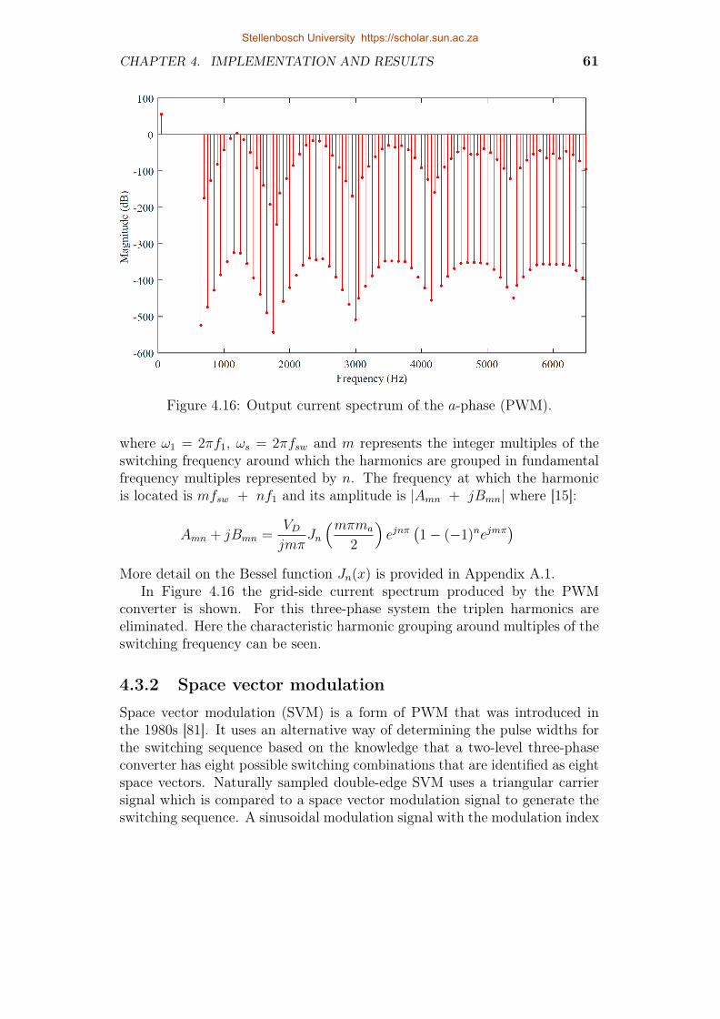
CHAPTER 4. IMPLEMENTATION AND RESULTS 61
Figure 4.16: Output current spectrum of the a-phase (PWM).
where ω1 = 2πf1, ωs = 2πfsw and m represents the integer multiples of theswitching frequency around which the harmonics are grouped in fundamentalfrequency multiples represented by n. The frequency at which the harmonicis located is mfsw + nf1 and its amplitude is |Amn + jBmn| where [15]:
Amn + jBmn =VDjmπ
Jn
(mπma
2
)ejnπ
(1− (−1)nejmπ
)More detail on the Bessel function Jn(x) is provided in Appendix A.1.
In Figure 4.16 the grid-side current spectrum produced by the PWMconverter is shown. For this three-phase system the triplen harmonics areeliminated. Here the characteristic harmonic grouping around multiples of theswitching frequency can be seen.
4.3.2 Space vector modulation
Space vector modulation (SVM) is a form of PWM that was introduced inthe 1980s [81]. It uses an alternative way of determining the pulse widths forthe switching sequence based on the knowledge that a two-level three-phaseconverter has eight possible switching combinations that are identified as eightspace vectors. Naturally sampled double-edge SVM uses a triangular carriersignal which is compared to a space vector modulation signal to generate theswitching sequence. A sinusoidal modulation signal with the modulation index
Stellenbosch University https://scholar.sun.ac.za

CHAPTER 4. IMPLEMENTATION AND RESULTS 62
ma as amplitude and the modulation angle φ added to the phase:
i∗abc = ma
sin(2πft+ φ)sin(2πft+ φ− 2π
3)
sin(2πft+ φ− 4π3
)
is modified to generate the space-vector equivalent modulation waveform [81]:
i∗mod = i∗abc −1
2(max(i∗abc) +min(i∗abc))
In Figure 4.17 the space-vector modulation waveform is compared to thetriangular carrier signal. For instance, intervals where the instantaneous valueof the modulation waveform is greater than the carrier signal, the switch stateis set to u = 1. In the opposite case the switch state becomes u = −1, as canbe seen in Figure 4.18.
Figure 4.17: Triangular carrier, space-vector modulation signal and sinusoidalwaveform generated to determine the switching pulse widths.
Figure 4.18: Space-vector modulated switching pulses.
Stellenbosch University https://scholar.sun.ac.za

CHAPTER 4. IMPLEMENTATION AND RESULTS 63
The frequency at which the harmonic is located is mfsw + nf1 and itsamplitude is |Amn + jBmn| where
A0n + jB0n|n>1 =
√3maVDπ
1
n+ 1
sin(
[n+ 1]π
6
)cos(
[n+ 1]π
2
)×√
3 + 2 cos(
[n+ 1]π
3+π
6
)
+1
n− 1
sin(
[n− 1]π
6
)cos(
[n− 1]π
2
)×√
3 + 2 cos(
[n− 1]π
3− π
6
)
for the baseband harmonics (m = 0, n > 1) [81]. More detail is provided onthe Bessel function Jn(x) in Appendix A.1. In the case of the carrier harmonics(m > 0, n = 0) and sideband harmonics (m > 0, n 6= 0) the next equation isused to determine the harmonic amplitudes [81]:
Amn + jBmn =
8VDmπ2
π
6sin(
[m+ n]π
2
)Jn
(m
3π
4ma
)+ 2 cosn
π
6Jn
(m
√3π
4ma
)
+1
nsinm
π
2cosn
π
2sinn
π
6
J0
(m
3π
4ma
)− J0
(m
√3π
4ma
)∣∣∣∣n6=0
+∞∑k=1k 6=−n
1
[n+ k]sin(
[m+ k]π
2
)cos(
[n+ k]π
2
)sin(
[n+ k]π
6
)×
Jk
(m
3π
4ma
)+ 2 cos
([2n+ 3k]
π
6
)Jk
(m
√3π
4ma
)
+∞∑k=1k 6=n
1
[n− k]sin(
[m+ k]π
2
)cos(
[n− k]π
2
)sin(
[n− k]π
6
)×
Jk
(m
3π
4ma
)+ 2 cos
([2n− 3k]
π
6
)Jk
(m
√3π
4ma
)
Figure 4.19 provides the spectrum of the converter’s space-vector
modulated grid-side current. In three-phase systems the triplen harmonics areeliminated. It can be seen that the harmonic content is concentrated aroundmultiples of the switching frequency, which is fsw = 1.2 kHz in this case.
Stellenbosch University https://scholar.sun.ac.za

CHAPTER 4. IMPLEMENTATION AND RESULTS 64
Figure 4.19: Output current spectrum obtained from space vector modulation.
4.4 Performance evaluation and comparisonThe suitability of the developed control approach is evaluated by comparingthe four control scenarios (MPC with a short horison of N = 1, MPC with along horison of N = 12, open-loop PWM-based control and naturally-sampledSVM) with a focus on compliance to the grid-code harmonic limits. Thesecontrol scenarios are evaluated at both a low switching frequency and a highswitching frequency. For the first set of results, all control approaches areevaluated at a switching frequency of 1.2 kHz while a sampling interval ofTs = 40µs is applied, equivalent to a sampling frequency of 25 kHz. Thesecond set is obtained with a switching frequency of 10.3 kHz, with a samplinginterval of Ts = 20µs, doubling the sampling frequency to 50 kHz. Thesteady-state response is observed at about t = 10s, and is shown over one50 Hz fundamental period. Each result includes the a-phase grid-side currentand its reference, corresponding switching sequence and performance againstthe harmonic limits. Each spectrum is calculated from 200 steady-statefundamental periods.
4.4.1 Performance at a low switching frequency
The results of the first set of simulations are presented in Figure 4.20 (MPCwith short horison), Figure 4.21 (MPC with long horison), Figure 4.22(naturally sampled open-loop PWM) and Figure 4.23 (naturally sampledSVM). Each of the four control approaches is adjusted to have a switchingfrequency of approximately 1.2 kHz. To achieve this for the N=1 and N=12
Stellenbosch University https://scholar.sun.ac.za

CHAPTER 4. IMPLEMENTATION AND RESULTS 65
cases, the weighting factor in the cost function was adjusted to λu = 0.8and λu = 2 respectively. For PWM and SVM the switching frequency isdirectly specified beforehand as fsw = 1.2 kHz. The pulse-width modulatedswitching sequence shown in Figure 4.22b, and the space vector modulatedsequence in Figure 4.23b is generated according to this switching frequency andremains constant for every fundamental period. This differs from MPC wherethe switching sequence varies throughout the simulation and the switchingfrequency is not fixed or constant. The switching frequency is thereforedetermined as an average and is limited to be fsw < fs/2, less than halfthe sampling frequency but not equal, as the controller does not change theswitch state during every single sampling instant.
A prediction horison of twelve time steps spans 480µs ahead of the currentposition in time, as opposed to the single 40µs time step. This enables thelong-horison approach to anticipate a better trade-off between the objectivesof switching reduction and reference tracking. Table 4.2 provides the trackingerror of the fundamental 50 Hz component I2(f1) for these approaches,calculated as follows using the amplitude of the reference current and theharmonic amplitude at f1 obtained from the fft of the grid current:
tracking error =
(I2(f1) − I2 ref
I2 ref
)× 100%
The tracking errors for the short- and long-horison MPC approaches are 1.74%and 0.53% respectively. This verifies that long-horison control provides anoptimised trade-off between control objectives by improving the tracking ofthe fundamental component with the same number of switching transitionstaking place. There is no tracking error provided for the open-loop PWM andnaturally-sampled SVM as the reference is calculated so that the tracking errorof the fundamental component is zero.
It is also seen that long-horison MPC offers lower total harmonic distortion(THD) than short-horison control with a THD of 2.3% versus 3.36%respectively, much less than the 7.93% and 5.03% distortion resulting fromPWM and SVM. This can be observed as the grid-current i2a in Figure 4.21ahas smaller ripple for the same number of switching transitions when controlledby MPC with the long prediction horison than with the short-horison controlin Figure 4.20a. The largest ripple is observed in the PWM-controlled outputcurrent in Figure 4.22a.
The South African NRS 079-2-1:2010 grid code [16] places limits on thegrid-current harmonic distortion at multiples of the fundamental frequency.These limits are expressed in terms of the harmonic amplitudes as percentagesof the fundamental component and are provided in Appendix A.2.
With classic control schemes such as PWM, the resulting spectrum consistsof discrete spectral lines grouped around multiples of the switching- orcarrier frequency. In Figure 4.22c the spectral content present around the24th harmonic multiple of the fundamental frequency, equivalent to the first
Stellenbosch University https://scholar.sun.ac.za

CHAPTER 4. IMPLEMENTATION AND RESULTS 66
(a) Grid-side current and reference
(b) Switching sequence
(c) Grid-side current harmonics compared to grid-code harmonic distortion limits
Figure 4.20: Results for the MPC short-horison (N = 1) case at fsw = 1.2 kHz.
Stellenbosch University https://scholar.sun.ac.za

CHAPTER 4. IMPLEMENTATION AND RESULTS 67
(a) Grid-side current and reference
(b) Switching sequence
(c) Grid-side current harmonics compared to grid-code harmonic distortion limits
Figure 4.21: Results for the MPC long-horison (N = 12) case at fsw = 1.2 kHz.
Stellenbosch University https://scholar.sun.ac.za

CHAPTER 4. IMPLEMENTATION AND RESULTS 68
(a) Grid-side current and reference
(b) Switching sequence
(c) Grid-side current harmonics compared to grid-code harmonic distortion limits
Figure 4.22: Results for the PWM case at fsw = 1.2 kHz.
Stellenbosch University https://scholar.sun.ac.za

CHAPTER 4. IMPLEMENTATION AND RESULTS 69
(a) Grid-side current and reference
(b) Switching sequence
(c) Grid-side current harmonics compared to grid-code harmonic distortion limits
Figure 4.23: Results for the SVM case at fsw = 1.2 kHz.
Stellenbosch University https://scholar.sun.ac.za

CHAPTER 4. IMPLEMENTATION AND RESULTS 70
Table 4.2: Summary of the simulation results
Weighting Tracking Grid-codeApproach factor λu error THD complianceTs = 40µs, fsw=1.2 kHz:MPC (N=1) 0.8 1.74% 3.36% NoMPC (N=12) 2 0.53% 2.30% NoPWM - - 7.93% NoSVM - - 5.03% NoTs = 20µs, fsw=10.3 kHz:MPC (N=1) 6× 10⁻⁴ 0.12% 0.27% NoMPC (N=12) 6× 10⁻⁷ 0.03% 0.19% YesPWM - - 0.87% YesSVM - - 0.56% Yes
multiple of the switching frequency, exceeds the harmonic limits on the 22ndand 26th harmonics, bearing in mind the absence of the triplen harmonicsin a three-phase system as discussed earlier. With SVM a similar trend isobserved in Figure 4.23c, but with more widely spread harmonic content ateven harmonic positions around the switching frequency, except at the triplenharmonics.
Model predictive control results in the spread of spectral content but stillshows a very slight concentration of content around multiples of the switchingfrequency. Due to some of the switching energy being converted to noise, theenergy is summed in 50 Hz frequency bands to obtain the discrete harmonicamplitudes at multiples of the fundamental frequency f1. The harmonicdistortion resulting from the long-horison approach, Figure 4.21c, is slightlylower than from the short-horison approach in Figure 4.20c, but both exceedthe limits on all higher-order harmonics: those surrounding the switchingfrequency (24th harmonic) and higher. Furthermore, both approaches alsoviolate restrictions on all the even harmonics in the lower-order range, withthe short-horisons approach exceeding limits on a few odd harmonics as well.
4.4.2 Performance at a high switching frequency
During the second set of results the performance of the four approaches(short-horison MPC in Figure 4.24; long-horison MPC in Figure 4.25;open-loop PWM in Figure 4.26) and naturally-sampled SVM in Figure 4.27)are investigated at a higher switching frequency of fsw = 10.3 kHz and asampling frequency of fs = 50 kHz. The weighting factor was adjustedto λu = 6×10⁻⁴ and λu = 6×10⁻⁷ for the short- and long-horison casesrespectively.
From Table 4.2 it is seen once more that MPC with long horisonsoutperforms MPC with short horisons through a lower tracking error and
Stellenbosch University https://scholar.sun.ac.za

CHAPTER 4. IMPLEMENTATION AND RESULTS 71
(a) Grid-side current and reference
(b) Switching sequence
(c) Grid-side current harmonics compared to grid-code harmonic distortion limits
Figure 4.24: Results for the MPC short-horison (N = 1) case at fsw = 10.3 kHz.
Stellenbosch University https://scholar.sun.ac.za

CHAPTER 4. IMPLEMENTATION AND RESULTS 72
(a) Grid-side current and reference
(b) Switching sequence
(c) Grid-side current harmonics compared to grid-code harmonic distortion limits
Figure 4.25: Results for the MPC long-horison (N = 12) case at fsw = 10.3 kHz.
Stellenbosch University https://scholar.sun.ac.za

CHAPTER 4. IMPLEMENTATION AND RESULTS 73
(a) Grid-side current and reference
(b) Switching sequence
(c) Grid-side current harmonics compared to grid-code harmonic distortion limits
Figure 4.26: Results for the PWM case at fsw = 10.3 kHz.
Stellenbosch University https://scholar.sun.ac.za

CHAPTER 4. IMPLEMENTATION AND RESULTS 74
(a) Grid-side current and reference
(b) Switching sequence
(c) Grid-side current harmonics compared to grid-code harmonic distortion limits
Figure 4.27: Results for the SVM case at fsw = 10.3 kHz.
Stellenbosch University https://scholar.sun.ac.za

CHAPTER 4. IMPLEMENTATION AND RESULTS 75
THD percentage. Both the tracking error and THD are much lower at a highswitching frequency than those obtained at the low switching frequency. Thegrid-side currents for all four scenarios are smooth with no noticeable ripple.
MPC with long horisons, PWM and SVM manage to perform within thegrid-code current-distortion limits. The grid-current spectrum produced byMPC with a short horison adheres to all harmonic limits, except at thetenth harmonic (500 Hz). This coincides with the resonant frequencies ofthe LCL-filter [14]:
fres1 =1
2π√CL2
and fres2 =1
2π
√C
L1L2
L1 + L2
,
which delivers fres1 = 493 Hz and fres2 = 512 Hz when substituting thefilter’s component values, provided in Table 4.1, into the equations. Throughthe application of a longer prediction horison the MPC controller managesto displace enough energy away from the filter’s resonant frequencies at thetenth harmonic to fully comply with the harmonic distortion limits. Thiseliminates the need for active damping (AD) of filter resonance (e.g.: throughvirtual resistance (VR)-based approaches [63; 82; 48; 47]) as required by linearcontrollers which make use of classic control techniques.
4.5 SummaryFigure 4.28 provides a glance on how this chapter relates to thosethat surround it. This chapter provides the evaluation of themodel-predictive direct current-control strategy developed in Chapter 3, fora three-phase grid-connected converter with LCL-filter by implementation ina MATLAB-based simulation for evaluation. A sphere decoding algorithm wasimplemented as a computationally efficient solver for the solution search. Themodel shows correct functioning as current controller, fast transient responseand good reference tracking of the fundamental 50 Hz component. Thesuitability of the current-control scheme for a grid-connected converter setupwas investigated by comparing it with open-loop PWM, naturally-sampledSVM, as well as the short- and long-horison application of the developed MPCscheme. The spectrum of the grid-side current was tested against the harmonicdistortion limits of the NRS 079-2-1:2010 grid code for current injected intothe grid. The evaluation was performed at both a low and a high switchingfrequency.
At low frequencies both MPC with short- and long-horison approaches shownon-compliance with the harmonic limits in the higher frequency range aroundthe switching frequency and onwards, as well as limits at even harmonics inthe lower frequency range. With an increase in switching frequency a pointis reached where the method manages to comply with the grid-code harmonic
Stellenbosch University https://scholar.sun.ac.za

CHAPTER 4. IMPLEMENTATION AND RESULTS 76
requirements, but this is at a much higher switching frequency than the rangethat is ideally intended for MPC to leverage its benefits from long horisons.One way the to reduce the switching frequency at which the controller functionssatisfactorily is to adjust or re-design the filter parameters.
MPC utilising long prediction horisons is able to anticipate future effectsof actuations and plan further in advance. From the results it was confirmedthat MPC with long horisons provides a more optimal trade-off betweenthe two control objectives, reference tracking and switching reduction, thanMPC with short horisons as it delivered better reference tracking and lowertotal harmonic distortion. It was also observed that long-horison controlautomatically attenuates the filter resonance to an acceptable level that fullycomplies with the grid code, eliminating the need for active damping techniquesused with linear controllers.
At high switching frequency it is clear that the method is currentlyoutperformed by PWM and SVM. Despite the control approach’s currentinadequacies, there is room for improvement through future research regardingharmonic performance.
Figure 4.28: Brief overview of the thesis chapters.
Stellenbosch University https://scholar.sun.ac.za

Chapter 5
Discussion and Conclusion
In this chapter a summary is given of the whole thesis and how the researchobjectives were met, where-after the main findings and recommendations forfuture research are made before the final conclusion is drawn.
5.1 Summary of the researchThe focus of the research is the development and evaluation of a MPCcurrent-control strategy for a three-phase grid-connected converter withLCL-filter. All of the research objectives were achieved during the study:
• A discrete-time state space model was derived that describes the grid-tiedconverter.
• The optimisation approach for MPC with long horisons as described in[46] was adapted and extended to incorporate the grid voltage.
• The following control objectives were incorporated into the cost function:
– To minimise current tracking error.
– To minimise switching frequency.
• A sphere decoding algorithm was described and implemented asa recursive function that solved the optimisation problem in acomputationally efficient manner.
• The developed control approach was implemented and evaluated byMATLAB-based simulations.
A review follows on each chapter to summarise the main points that wereaddressed in the thesis and how they support the objectives of the study.
77
Stellenbosch University https://scholar.sun.ac.za

CHAPTER 5. DISCUSSION AND CONCLUSION 78
5.1.1 Chapter 1
The first chapter introduced the background and context of the research, statedthe main focus and objectives of the thesis and provided a roadmap of the thesischapters.
5.1.2 Chapter 2
A literature review was conducted to provide an understanding of andbackground on the history and applications of power converters. Aclassification and discussion was provided on the types of control methods thatare applied to power converters, followed by a discussion on the suitabilityof predictive control methods to present-day control systems and powerconverters. The specific types of predictive control methods and specificallymodel predictive control (MPC), its benefits, drawbacks and basic concepts,were discussed. A review was done on existing research relevant to modelpredictive control of grid-tied converters.
5.1.3 Chapter 3
In Chapter 3 the three-phase system and the proposed controller are describedand developed mathematically by defining the constraints of the finite controlset regarding the integer switch states, and deriving a state-space model thatcan be used to describe and predict the behaviour of the system according toits inputs, hereby achieving the first objective.
This model differs from that developed in [46] as within the state-spaceequation the grid voltage is considered as an additional input vector alongsidethe switch-state input vector, rather than being included in the state vectoras is the general trend in [47; 48]. This meant that the algebra of the standardMPC optimisation approach be reworked to accommodate the inclusion of thegrid voltage as an input vector and this achieved the second objective of theresearch.
For the third objective a cost function was formulated to include twoweighted control objectives, namely reducing reference tracking error andsecondly switching frequency reduction as a means to reduce losses in theconverter. This cost function was used to evaluate the optimality of availableswitching actions, as the option that minimises the cost is the most optimal.The state-space equation was used to predict the future behaviour of thesystem according to a specific sequence of switching states applied. Thecost of each switch action was summed over the prediction horison of N timesteps to give the overall cost of a specific switching-sequence. The number ofpossible sequences and their predicted outcomes increased exponentially thelonger the chosen horison length, posing an exhaustive search computationallyif every available sequence was to be evaluated. The minimisation of the
Stellenbosch University https://scholar.sun.ac.za

CHAPTER 5. DISCUSSION AND CONCLUSION 79
cost function was rewritten to become an integer least-squares (ILS) problemwith the switching sequence vector U(k) as the optimisation variable, and atransformation matrix H necessary to generate the discrete solutions spacewherein all candidate solutions U(k) were mapped.
In fulfilment of the fourth objective sphere decoding was incorporated as anefficient solver of the ILS-problem at a long prediction horison that inherentlyhas an exponentially enlarging/extending set of candidate solutions. Thesphere decoder approaches the ILS-problem as a minimisation of the Euclideandistance between its central point (position of the unconstrained solution)and candidate solutions in the solution space. The closer the solution lies tothe sphere’s center, the more optimal it is. A Babai estimate of what themost optimal solution might be is used as the starting point of the search toexclude as many sub-optimal solution points from the search as possible. Asthe sphere decoder explores the nodes of the search tree, it either prunes thebranch if its Euclidean distance falls outside of the sphere’s radius, or advancesalong the branch to the next node to repeat the evaluation. Once it reachesa complete set of actuations at the bottom of the tree that fall within theradius, it considers it as a new temporary optima and tightens the radius tothat candidate’s distance from the sphere’s center. The decoder proceeds inthis manner until only one candidate remains in the sphere, which is thenselected as the official optimal solution.
5.1.4 Chapter 4
In the fourth chapter the fifth objective which entails the implementationand evaluation of the MPC control scheme for the three-phase grid-connectedconverter with LCL-filter is addressed. The first part of the chapter describeshow the mathematical model developed in Chapter 3 was implemented in aMATLAB-based simulation. A flow diagram is used to describe the logical flowwithin the main function script that simulates the grid-connected converterwith LCL-filter and how control is performed by the MPC strategy. Analgorithm is formulated to perform the sphere decoding from program codeand is implemented as a recursive function written in a separate MATLABscript and called from within the main MPC function to perform the optimisedsearch. The efficiency of the sphere decoder is evaluated by counting thenumber of floating point operations (FLOPS) performed during the solutionsearch and comparing them to the FLOPS performed during an exhaustivesearch at different prediction horison lengths N . The use of the sphere decoderenables a horison length of N = 15 to be used during the simulation, whereasthe exhaustive search limited the simulation to a prediction horison of N = 8time steps due to its computational burden.
Sample output from the simulation, such as the capacitor voltage, inverter-and grid-side current waveforms, are investigated to verify that the MPCcontroller model and its implementation in the simulation was functioning
Stellenbosch University https://scholar.sun.ac.za

CHAPTER 5. DISCUSSION AND CONCLUSION 80
correctly. The dynamic response was also tested by insertion of a step in thereference amplitude, to which the controller adjusted very quickly. Thereafteran explanation was given on how the spectral content of the grid-side currentwas determined from the simulation’s time-domain results to obtain thediscrete harmonics and THD.
After the explanation of how the simulation was developed for the MPCand sphere decoder’s implementation, detail regarding the implementationof an open-loop PWM controller and space vector modulator for the samethree-phase grid-connected converter is given, such as generation of themodulated switching signals and calculation of the spectrum by using theFourier series expansion and Bessel function.
In the second part of the chapter an evaluation is provided of thedeveloped current control scheme through a comparison of the following controlapproaches: MPC with a short horison, MPC with a long horison, open-loopnaturally-sampled PWM and SVM. These approaches were each evaluated ata low switching frequency and a high switching frequency. Attributes suchas tracking error of the fundamental 50 Hz component and total harmonicdistortion are also compared.
At low switching frequencies the developed MPC scheme exceeds asignificant number of harmonic limits predominantly at even harmonics, thusnot providing satisfactory performance according to the NRS 079-2-1:2010grid-code current distortion limits. With an increase in switching frequencya point is reached where the long-horison approach manages to comply withthe grid-code harmonic requirements, but this is at a much higher switchingfrequency than the range that is ideally intended for MPC to leverage thebenefits of long horisons. A more detailed breakdown of the findings follows.
5.2 Main findingsThe model and simulation developed of the MPC scheme functions correctly:
• The controller is able to track the fundamental 50 Hz component withaccuracy.
• The controller has fast transient response as it reacts quickly toabrupt changes in the reference by fully adjusting within less than twomilliseconds with little overshoot.
The sphere decoder was proven to provide a significant efficiency improvementover an exhaustive search approach.
Stellenbosch University https://scholar.sun.ac.za

CHAPTER 5. DISCUSSION AND CONCLUSION 81
MPC performs better using long-horison control than with short-horisoncontrol:
• Long-horison control automatically attenuates LCL-filter resonancepresent in short-horison control without the use of active dampingtechniques generally used in linear controllers. It is able to displacesome of the switching energy away from the resonant frequencies of theLCL-filter.
• Long-horison control is able to anticipate and prepare for a inserted stepin amplitude a number of time steps ahead due to its prediction horisonspanning further into the future than in the short-horison case.
• Long-horison control shows smaller reference-tracking error whencompared to short horisons when compared at the same switchingfrequency, it is therefore able to optimise the switching sequence toreduce tracking error using the same number of switching transitions.
• Long-horison control provides lower overall THD and smaller ripple inthe grid-side current than short-horison control, open-loop PWM andSVM when compared at the same switching frequency.
Performance against the NRS 079-2-1:2010 grid code harmonic distortion limitsand the traditional PWM-type approaches:
• It is observed that MPC produces less ripple in the grid-side currentat both short and long horisons than PWM with the same switchingfrequency. PWM has a fixed switching frequency and pulse-widthmodulated switching sequence throughout, whereas MPC offers moreflexibility of the switching frequency as it is able to constantly optimiseand adapt the switching sequence to provide an optimal trade-offaccording to the desired control objectives and their priority weightingswithin the cost function.
• PWM and SVM approaches do not comply to the grid code harmoniclimits when the switching frequency and its surrounding harmoniccontent falls within the range of the grid code (0 Hz - 1.7 kHz).
• At a low switching frequency MPC does not comply with the currentdistortion harmonic limits at even harmonics, nor at harmonics higherthan the switching frequency.
• At a high switching frequency long-horison MPC is able to comply withthe grid-code harmonic distortion limits, however short-horison controlfalls short of compliance to the harmonic limit at the filter resonancefrequency.
Stellenbosch University https://scholar.sun.ac.za

CHAPTER 5. DISCUSSION AND CONCLUSION 82
5.3 Suggestions for future research• Further work can be done on the control approach to improve the
performance regarding even and higher-order harmonics in order tocomply with the distortion limits of the grid code. [83] uses the concept ofa spectrogram, which is the squared magnitude of the short-time Fouriertransform (STFT). The MPC scheme applies spectrogram constraints tothe output spectrum across multiple time steps of the prediction horison.Spectrogram MPC is able to enforce hard constraints on the spectrum,hereby differing from the frequency-weighted methods incorporated withMPC such as band-pass filters [84] and high-pass Butterworth filters [85],where the high frequency behaviour is penalised and fine-tuned in thecost function.
• Improvement in the design of the filter should be investigated. Switchingat lower frequencies will require a larger filter, as a larger converter-sideinductor reduces current ripple, and the larger the filter capacitor, themore current ripple goes through the capacitor instead of the utilitynetwork. The drawbacks related to these parameter adjustments areincreased component size and cost. One way of reducing distortion couldbe to extend the LCL-filter, but this significantly increases the controlcomplexity, could imply a larger input voltage requirement and increasesthe system cost.
• Further research can be done regarding the practical implementation ofthe controller for long horisons to restrict the computational time neededfor each time step / sampling period. A reduction is needed from severalminutes taken in simulation to the several microseconds needed in realtime by a practical implementation.
5.4 ConclusionDuring the research the suitability of a direct model predictive currentcontrol strategy for a three-phase grid-connected converter with LCL-filter wasevaluated. The control objectives entailed minimising current-tracking errorand switching frequency. The research contributed to knowledge creation inthe field of model predictive control (MPC) in power electronics by extendingon the work done in [46] by incorporating the grid voltage as an input vectorin the mathematical model and optimisation approach.
A sphere decoder was incorporated in order to relieve the computationalburden related to an exhaustive search, by improving the efficiency by whichthe simulation executes a solution search. This makes it possible to use longprediction horisons of up to fifteen time steps during the simulation approach.
Stellenbosch University https://scholar.sun.ac.za

CHAPTER 5. DISCUSSION AND CONCLUSION 83
The performance when using MPC with short horisons versus long horisonswas investigated and compared to an open-loop pulse-width modulationcontroller, evaluated at both a low and high switching frequency. Thedeveloped controller provided accurate current-reference tracking and fasttransient response for both short and long horisons, however it was noticed thatlong-horison control is clearly superior and automatically damps the resonantfrequencies of the filter. At low switching frequencies the controlled grid-sidecurrent does however not fully comply with the harmonic distortion limitsspecified by the South African grid code. The odd harmonics are generallywithin the specified limits, but the even harmonics requires improvement. Thisstrategy is therefore not suitable for grid-tied inverter applications, howeverfuture research can be done to develop methods to suppress the even andhigh-order harmonics. The use of longer horisons improves performance butthere is an increased computational burden which is a barrier to simulationefforts and practical implementation.
In the past the adoption of MPC was limited by the computational abilitiesat the time, today it is possible to implement such a controller in simulationand perform predictions and optimisation over long horisons [10; 11; 46].The increasing rate at which technology and computational power advancesprovides a prospect that the practical implementation of long-horison MPCcontrollers will become feasible in the near future.
Stellenbosch University https://scholar.sun.ac.za

Appendices
84
Stellenbosch University https://scholar.sun.ac.za

Appendix A
Additional Theory
A.1 Bessel functionBessel function of the first type [15]:
Jnx =1
2π
∫ π
−πej(xsiny−ny)dy
Characteristics:
Jn−x = (−1)nJn(x)
J−n(x) = (−1)nJn(x)
Figure A.1: Output of a first order Bessel function. [15].
85
Stellenbosch University https://scholar.sun.ac.za

APPENDIX A. ADDITIONAL THEORY 86
A.2 Grid codeThe NRS 097-2-1:2010 [16] currently serves as the grid code to facilitate theinterconnection of renewable energy sources to the national utility grid in SouthAfrica. Herein harmonic distortion limits are specified for current injectedinto the grid. Low current-distortion levels prevent harmful effects on otherequipment connected to the grid. In accordance with the IEC 61727:2004the individual harmonics have to comply with the percentages provided inTable A.1:
Table A.1: Current distortion limits according to harmonics [16].
Odd harmonics Distortion limit3rd through 9th Less than 4.0%
11th through 15th Less than 2.0%17th through 21st Less than 1.5%23rd through 33rd Less than 0.6%Even harmonics Distortion limit
2nd through 8th Less than 1.0%10th through 32nd Less than 0.5%
Stellenbosch University https://scholar.sun.ac.za

List of References
[1] International Energy Agency and International Energy Agency Staff: Electric-ity Information 2002: With 2001 Data. IEA Statistics. OECD, InternationalEnergy Agency, 9 Rue de la Fédération, 75015 Paris, France, 2002. ISBN 978-92-64-19793-0.
[2] International Energy Agency and International Energy Agency Staff: Electric-ity Information 2010: With 2009 Data. IEA Statistics. OECD, InternationalEnergy Agency, 9 Rue de la Fédération, 75015 Paris, France, 2010. ISBN 978-92-64-08418-6.
[3] International Energy Agency and International Energy Agency Staff: Electric-ity Information 2017: With 2016 Data. IEA Statistics. OECD, InternationalEnergy Agency, 9 Rue de la Fédération, 75015 Paris, France, 2017. ISBN 978-92-64-27812-7.
[4] Walwyn, D. and Brent, A.: Renewable energy gathers steam in south africa.Renewable and Sustainable Energy Reviews, vol. 41, pp. 390–401, 2015.
[5] PV insights: Solar PV wafer weekly spot price. 2013.
[6] Brown, A., Müller, S. and Dobrotkova, Z.: Renewable energy: Markets andprospects by technology. IEA information paper, 2011.
[7] Bull, S.: Renewable energy today and tomorrow. Proceedings of the IEEE,vol. 89, no. 8, pp. 1216–1226, 2001.
[8] Al Qamer: Solar (PV). [Online], 2016. Retrieved on 30/09/2017.Available at: http://www.alqamer.com/index.php/2016-02-01-19-25-41/solar-pv
[9] Lai, W.F., Chen, S.M., Liang, T.J., Lee, K.W. and Ioinovici, A.: Design andimplementation of grid connection photovoltaic micro inverter. In: 2012 IEEEEnergy Conversion Congress and Exposition (ECCE), pp. 2426–2432. Sept 2012.ISSN 2329-3721.
[10] Rodriguez, J. and Cortes, P.: Predictive Control of Power Converters and Elec-trical Drives, pp. 3–39. Wiley-IEEE Press, 2012. ISBN 9781119963981.
[11] Cortes, P., Kazmierkowski, M.P., Kennel, R.M., Quevedo, D.E. and Rodriguez,J.: Predictive control in power electronics and drives. IEEE Transactions onIndustrial Electronics, vol. 55, no. 12, pp. 4312–4324, Dec 2008. ISSN 0278-0046.
87
Stellenbosch University https://scholar.sun.ac.za

LIST OF REFERENCES 88
[12] Geyer, T.: Model Predictive Control of High Power Converters and IndustrialDrives. Wiley, 2016. ISBN 9781119010869.Available at: https://books.google.co.za/books?id=KtgQDQAAQBAJ
[13] Karamanakos, P., Geyer, T. and Kennel, R.: Reformulation of the long-horizondirect model predictive control problem to reduce the computational effort. In:2014 IEEE Energy Conversion Congress and Exposition (ECCE), pp. 3512–3519. Sept 2014. ISSN 2329-3721.
[14] Miranda, H., Teodorescu, R., Rodriguez, P. and Helle, L.: Model predictivecurrent control for high-power grid-connected converters with output LCL-filter.In: 2009 35th Annual Conference of IEEE Industrial Electronics, pp. 633–638.Nov 2009. ISSN 1553-572X.
[15] Du Toit Mouton, H: Power electronics. University of Stellenbosch, 2014.
[16] Eskom Standardization Section: Grid interconnection of embedded generation,Part 2, Section 1. World Energy Council, Pretoria, Republic of South Africa,2010. ISBN 978-0-626-25101-7.
[17] Tiwari, G. and Mishra, R.: Advanced Renewable Energy Sources. Royal Societyof Chemistry, 2015. ISBN 9781782625780.
[18] qing Yuan, Q., jie Wu, X., ting Zhang, T. and an Wang, K.: Model predictivecontrol for the high-power grid-connecting pwm converters. In: 2013 Interna-tional Conference on Electrical Machines and Systems (ICEMS), pp. 252–256.Oct 2013.
[19] U.S. Energy Information Administration: International Energy Outlook 2016.Office of Energy Analysis, U.S. Department of Energy, Washington, DC 20585,2016.
[20] for Economic Co-Operation, O. and Development: World Energy Outlook 2017.OECD, 2017. ISBN 978-92-64-28205-6.
[21] for Economic Co-Operation, O. and Development: World Energy Outlook 2016.OECD, 2016. ISBN 978-92-64-26494-6.
[22] Abbey, C., Robinson, J. and Joos: Integrating renewable energy sources andstorage into isolated diesel generator supplied electric power systems. In: 200813th International Power Electronics and Motion Control Conference, pp. 2178–2183. 2008.
[23] Yaramasu, V. and Wu, B.: Model Predictive Control of Wind Energy Conver-sion Systems. IEEE Press Series on Power Engineering. Wiley, 2016. ISBN9781118988589.
[24] Secretariat, UNFCCC: Report of the Conference of the Parties on its fifteenthsession, held in Copenhagen from 7 to 19 December 2009. In: United NationsFramework Convention on Climate Change. 2009.
Stellenbosch University https://scholar.sun.ac.za

LIST OF REFERENCES 89
[25] Li, Y., Agelidis, V.G. and Shrivastava, Y.: Wind-solar resource complementarityand its combined correlation with electricity load demand. In: 2009 4th IEEEConference on Industrial Electronics and Applications, pp. 3623–3628. 2009.
[26] Secretariat, UNFCCC: Report of the Conference of the Parties on its twenty-first session, held in Paris from 30 November to 13 December 2015. In: UnitedNations Framework Convention on Climate Change. 2015.
[27] South Africa, Department of Energy: State of Renewable Energy in SouthAfrica. Department of Energy (DOE), Pretoria, South Africa, 2015. ISBN978-1-920435-08-0.
[28] Baker, L.: The evolving role of finance in South Africa’s renewable energy sector.Geoforum, vol. 64, pp. 146–156, 2015.
[29] Eberhard, A.: The future of South African coal: Market, investment and pol-icy challenges. Program on Energy and Sustainable Development, vol. 100, pp.1–44, 2011.Available at: http://pesd.fsi.stanford.edu/sites/default/files/WP_100_Eberhard_Future_of_South_African_Coal.pdf
[30] Eskom: Coal power. [Online], 2017. Retrieved on 15/10/2017.Available at: http://www.eskom.co.za/AboutElectricity/ElectricityTechnologies/Pages/Coal_Power.aspx
[31] World Energy Council (WEC): World Energy Resources: 2013 Survey. WorldEnergy Council, London, 2013. ISBN 978-0-946121-29-8.
[32] South Africa, Department of Minerals and Energy: White Paper on the EnergyPolicy of the Republic of South Africa. Department of Minerals and Energy,Pretoria, South Africa, 1998. ISBN 0-9584235-8-X.
[33] Fawkes, H.: Energy efficiency in south african industry. Journal of Energy inSouthern Africa, vol. 16, no. 4, pp. 18–25, 2005.
[34] Davidson, O., Winkler, H., Kenny, A., Prasad, G., Nkomo, J., Sparks, D.,Howells, M. and Alfstad, T.: Energy policies for sustainable development inSouth Africa: Options for the future. Energy Research Centre, University ofCape Town, Cape Town, South Africa, 2006. ISBN 0-620-36294-4.
[35] Nakumuryango, A. and Inglesi-Lotz, R.: South Africa’s performance on renew-able energy and its relative position against the oecd countries and the rest ofAfrica. Renewable and Sustainable Energy Reviews, vol. 56, pp. 999–1007, 2016.
[36] McCrone, A., Moslener, U., d’Estais, F., Usher, E. and Grüning, C.: Globaltrends in renewable energy investment 2016. Frankfurt School of Finance &Management:, Frankfurt, Germany, 2016.
[37] Twidell, J. and Weir, T.: Renewable Energy Resources. 3rd edn. Taylor &Francis, 2015. ISBN 9781317660378.
Stellenbosch University https://scholar.sun.ac.za

LIST OF REFERENCES 90
[38] Agudelo-Vera, C., Mels, A., Keesman, K. and Rijnaarts, H.: Resource manage-ment as a key factor for sustainable urban planning. Journal of environmentalmanagement, vol. 92, no. 10, pp. 2295–2303, 2011.
[39] Ponting, C.: A New Green History of the World: The Environment and theCollapse of Great Civilizations. Penguin Books, 2007. ISBN 0-14-303898-2.
[40] Diamond, J.: Collapse: How societies choose to fail or succeed. Penguin, 2005.ISBN 0-670-03337-5.
[41] Castellano, J., Ribera, A. and Ciurana, J.: Integrated system approach to eval-uate social, environmental and economics impacts of buildings for users of hous-ings. Energy and Buildings, vol. 123, pp. 106–118, 2016.
[42] Ellabban, O., Abu-Rub, H. and Blaabjerg: Renewable energy resources: Cur-rent status, future prospects and their enabling technology. Renewable andSustainable Energy Reviews, vol. 39, pp. 748–764, 2014.
[43] Ahlfeldt, C., Brent, A., Gumede, D., Guy, D., Mosdell, S., Skeen, J., Spencer,F. and Thompson-Smeddle, L.: A South African Renewable Energy Guide ForLocal Government. Juta, Juta & Company Ltd, First Floor, Sunclare Building,21 Dreyer Street, Claremont, 7708, 2012. ISBN 9780702186929.
[44] Louwerse, M. and Van Peer, W.: Thematics: Interdisciplinary Studies. Converg-ing Evidence in Language and Communication Research Series. John BenjaminsPublishing Company, 2002. ISBN 9781588112828.
[45] Femia, N., Petrone, G., Spagnuolo, G. and Vitelli, M.: Power Electronics andControl Techniques for Maximum Energy Harvesting in Photovoltaic Systems.Industrial Electronics. CRC Press, 2017. ISBN 9781351832427.
[46] Geyer, T. and Quevedo, D.E.: Multistep finite control set model predictivecontrol for power electronics. IEEE Transactions on Power Electronics, vol. 29,no. 12, pp. 6836–6846, Dec 2014.
[47] Scoltock, J., Geyer, T. and Madawala, U.: Model Predictive Direct Power Con-trol for a grid-connected converter with an LCL-filter. In: Industrial Technology(ICIT), 2013 IEEE International Conference on, pp. 588–593. Feb 2013.
[48] Scoltock, J., Geyer, T. and Madawala, U.K.: A Model Predictive Direct CurrentControl strategy with predictive references for MV grid-connected converterswith LCL-filters. IEEE Transactions on Power Electronics, vol. 30, no. 10, pp.5926–5937, Oct 2015. ISSN 0885-8993.
[49] Code, G.: High and extra high voltage, e. on netz gmbh bayreuth, germany,april 2006.
[50] Carrasco, J.M., Franquelo, L.G., Bialasiewicz, J.T., Galvan, E., PortilloGu-isado, R.C., Prats, M.A.M., Leon, J.I. and Moreno-Alfonso, N.: Power-electronic systems for the grid integration of renewable energy sources: A survey.
Stellenbosch University https://scholar.sun.ac.za

LIST OF REFERENCES 91
IEEE Transactions on Industrial Electronics, vol. 53, no. 4, pp. 1002–1016, June2006. ISSN 0278-0046.
[51] Takahashi, I. and Noguchi, T.: A new quick-response and high-efficiency controlstrategy of an induction motor. IEEE Transactions on Industry Applications,vol. IA-22, no. 5, pp. 820–827, Sept 1986. ISSN 0093-9994.
[52] Ohnishi, T.: Three phase pwm converter/inverter by means of instantaneousactive and reactive power control. In: Industrial Electronics, Control and In-strumentation, 1991. Proceedings. IECON’91., 1991 International Conferenceon, pp. 819–824. IEEE, 1991.
[53] Holtz, J.: Pulsewidth modulation for electronic power conversion. Proceedingsof the IEEE, vol. 82, no. 8, pp. 1194–1214, 1994.
[54] Blaschke, F.: The principle of field orientation as applied to the new transvektorclosed-loop control system for rotating field machines. 1972.
[55] Kazmierkowski, M.P. and Malesani, L.: Current control techniques for three-phase voltage-source pwm converters: a survey. IEEE Transactions on industrialelectronics, vol. 45, no. 5, pp. 691–703, 1998.
[56] Siwakoti, Y.P., Peng, F.Z., Blaabjerg, F., Loh, P.C., Town, G.E. and Yang,S.: Impedance-source networks for electric power conversion part ii: Review ofcontrol and modulation techniques. IEEE Transactions on Power Electronics,vol. 30, no. 4, pp. 1887–1906, April 2015. ISSN 0885-8993.
[57] Garcia, C.E., Prett, D.M. and Morari, M.: Model predictive control: theoryand practice survey. Automatica, vol. 25, no. 3, pp. 335–348, 1989.
[58] Karamanakos, P., Geyer, T., Mouton, T. and Kennel, R.: Computationallyefficient sphere decoding for long-horizon direct model predictive control. In:2016 IEEE Energy Conversion Congress and Exposition (ECCE), pp. 1–8. Sept2016.
[59] Hassibi, B. and Vikalo, H.: On the sphere-decoding algorithm i. expected com-plexity. IEEE Transactions on Signal Processing, vol. 53, no. 8, pp. 2806–2818,Aug 2005. ISSN 1053-587X.
[60] Quevedo, D.E., Aguilera, R.P. and Geyer, T.: Predictive control in power elec-tronics and drives: Basic concepts, theory, and methods. In: Advanced and In-telligent Control in Power Electronics and Drives, pp. 181–226. Springer, 2014.
[61] Scoltock, J., Geyer, T. and Madawala, U.K.: A Model Predictive Direct CurrentControl strategy with predictive references for MV grid-connected converterswith LCL-filters. IEEE Transactions on Power Electronics, vol. 30, no. 10, pp.5926–5937, Oct 2015. ISSN 0885-8993.
Stellenbosch University https://scholar.sun.ac.za

LIST OF REFERENCES 92
[62] Mariethoz, S., Beccuti, A.G. and Morari, M.: Analysis and optimal currentcontrol of a voltage source inverter connected to the grid through an LCL-filter.In: 2008 IEEE Power Electronics Specialists Conference, pp. 2132–2138. June2008. ISSN 0275-9306.
[63] Panten, N., Hoffmann, N. and Fuchs, F.W.: Finite Control Set Model Predic-tive Current Control for Grid-Connected Voltage-Source Converters with LCL-filters: A study based on different state feedbacks. IEEE Transactions on PowerElectronics, vol. 31, no. 7, pp. 5189–5200, July 2016. ISSN 0885-8993.
[64] Maccari, L.A., Montagner, V.F. and Lima, D.M.: Model predictive current con-troller applied to grid-connected LCL-filters. In: 2016 12th IEEE InternationalConference on Industry Applications (INDUSCON), pp. 1–6. Nov 2016.
[65] Yoo, D.K., Wang, L., Rogers, E. and Paszke, W.: Model predictive control ofthree phase voltage source converters with an LCL-filter. In: 2014 IEEE 23rdInternational Symposium on Industrial Electronics (ISIE), pp. 562–567. June2014. ISSN 2163-5137.
[66] Pena-Alzola, R., Liserre, M., Blaabjerg, F., Sebastián, R., Dannehl, J. andFuchs, F.W.: Analysis of the passive damping losses in LCL-filter-based gridconverters. IEEE Transactions on Power Electronics, vol. 28, no. 6, pp. 2642–2646, 2013.
[67] Bierhoff, M.H. and Fuchs, F.W.: Active damping for three-phase pwm rectifierswith high-order line-side filters. IEEE Transactions on Industrial Electronics,vol. 56, no. 2, pp. 371–379, 2009.
[68] Rodriguez, J., Kazmierkowski, M.P., Espinoza, J.R., Zanchetta, P., Abu-Rub,H., Young, H.A. and Rojas, C.A.: State of the art of finite control set modelpredictive control in power electronics. IEEE Transactions on Industrial Infor-matics, vol. 9, no. 2, pp. 1003–1016, May 2013. ISSN 1551-3203.
[69] Rodriguez, J., Pontt, J., Silva, C.A., Correa, P., Lezana, P., Cortés, P. andAmmann, U.: Predictive current control of a voltage source inverter. IEEETransactions on Industrial Electronics, vol. 54, no. 1, pp. 495–503, 2007.
[70] Geyer, T. and Quevedo, D.E.: Performance of multistep finite control set modelpredictive control for power electronics. IEEE Transactions on Power Electron-ics, vol. 30, no. 3, pp. 1633–1644, March 2015. ISSN 0885-8993.
[71] Geyer, T., Papafotiou, G. and Morari, M.: Model predictive direct torquecontrol-part 1: Concept, algorithm, and analysis. IEEE Transactions on In-dustrial Electronics, vol. 56, no. 6, pp. 1894–1905, 2009.
[72] Geyer, T.: Low complexity model predictive control in power electronics andpower systems. Cuvillier Verlag, 2005.
Stellenbosch University https://scholar.sun.ac.za

LIST OF REFERENCES 93
[73] Papafotiou, G., Kley, J., Papadopoulos, K.G., Bohren, P. and Morari, M.:Model predictive direct torque control-part 2: Implementation and experimen-tal evaluation. IEEE Transactions on Industrial Electronics, vol. 56, no. 6, pp.1906–1915, 2009.
[74] Geyer, T.: Generalized model predictive direct torque control: Long predictionhorizons and minimization of switching losses. In: Decision and Control, 2009held jointly with the 2009 28th Chinese Control Conference. CDC/CCC 2009.Proceedings of the 48th IEEE Conference on, pp. 6799–6804. IEEE, 2009.
[75] Geyer, T.: A comparison of control and modulation schemes for medium-voltagedrives: Emerging predictive control concepts versus pwm-based schemes. IEEETransactions on Industry Applications, vol. 47, no. 3, pp. 1380–1389, 2011.
[76] Scoltock, J., Geyer, T. and Madawala, U.: Model Predictive Direct CurrentControl for a grid-connected converter: LCL-filter versus L-filter. In: 2013IEEE International Conference on Industrial Technology (ICIT), pp. 576–581.Feb 2013.
[77] Geyer, T.: Model predictive direct current control: Formulation of the sta-tor current bounds and the concept of the switching horizon. IEEE IndustryApplications Magazine, vol. 18, no. 2, pp. 47–59, 2012.
[78] Sternberg, S.: Dynamical systems, pp. 201 – 202. Courier Corporation, 2010.
[79] Karamanakos, P., Geyer, T. and Kennel, R.: Reformulation of the long-horizondirect model predictive control problem to reduce the computational effort. In:2014 IEEE Energy Conversion Congress and Exposition (ECCE), pp. 3512–3519. Sept 2014. ISSN 2329-3721.
[80] Transmission and Distribution Committee of the IEEE Power Engineering So-ciety: IEEE Std 519-1992, Recommended Practices and Requirements for Har-monic Control in Electrical Power Systems. IEEE, New York, United States ofAmerica, 2004. ISBN 1-55937-239-7.
[81] Holmes, D.G. and Lipo, T.A.: Pulse width modulation for power converters:principles and practice, vol. 18. John Wiley & Sons, 2003. ISBN 978-0-471-20814-3.
[82] Scoltock, J., Geyer, T. and Madawala, U.: Model Predictive Direct CurrentControl for a grid-connected converter: LCL-filter versus L-filter. In: IndustrialTechnology (ICIT), 2013 IEEE International Conference on, pp. 576–581. Feb2013.
[83] Hours, J., Zeilinger, M., Gondhalekar, R. and Jones, C.: Spectrogram-MPC:Enforcing hard constraints on systems’ output spectra. In: 2012 AmericanControl Conference (ACC), pp. 2010–2017. 2012. ISSN 0743-1619.
[84] Cortes, P., Rodriguez, J., Quevedo, D. and Silva, C.: Predictive current controlstrategy with imposed load current spectrum. IEEE Transactions on PowerElectronics, vol. 23, no. 2, pp. 612–618, 2008.
Stellenbosch University https://scholar.sun.ac.za

LIST OF REFERENCES 94
[85] Wills, A., Bates, D., Fleming, A., Ninness, B. and Moheimani, S.: Model predic-tive control applied to constraint handling in active noise and vibration control.IEEE Transactions on Control Systems Technology, vol. 16, no. 1, pp. 3–12,2008.
Stellenbosch University https://scholar.sun.ac.za