Model-based assignment and inferenceof protein backbone nuclear magnetic resonances.

Olga Vitek∗ Jan Vitek† Bruce Craig∗ Chris Bailey-Kellogg†‡

Abstract

Nuclear Magnetic Resonance (NMR) spectroscopy is a key experimental techniqueused to study protein structure, dynamics, and interactions. NMR methods face thebottleneck of spectral analysis, in particular determining the resonance assignment,which helps define the mapping between atoms in the protein and peaks in the spectra.A substantial amount of noise in spectral data, along with ambiguities in interpretation,make this analysis a daunting task, and there exists no generally accepted measure ofuncertainty associated with the resulting solutions. This paper develops a model-based inference approach that addresses the problem of characterizing uncertainty inbackbone resonance assignment. We argue that NMR spectra are subject to randomvariation, and ignoring this stochasticity can lead to false optimism and erroneousconclusions. We propose a Bayesian statistical model that accounts for various sourcesof uncertainty and provides an automatable framework for inference. While assignmenthas previously been viewed as a deterministic optimization problem, we demonstratethe importance of considering all solutions consistent with the data, and develop analgorithm to search this space within our statistical framework. Our approach is able tocharacterize the uncertainty associated with backbone resonance assignment in severalways: 1) it quantifies of uncertainty in the individually assigned resonances in terms oftheir posterior standard deviations; 2) it assesses the information content in the datawith a posterior distribution of plausible assignments; and 3) it provides a measureof the overall plausibility of assignments. We demonstrate the value of our approachin a study of experimental data from two proteins, Human Ubiquitin and Cold-shockprotein A from E. coli. In addition, we provide simulations showing the impact ofexperimental conditions on uncertainty in the assignments.

Keywords: Nuclear Magnetic Resonance (NMR) spectroscopy; uncertainty in NMRspectra; Bayesian modeling; statistical inference; protein structure; structural genomics

∗Dept. of Statistics, Purdue University.†Dept. of Computer Sciences, Purdue University.‡Corresponding author: cbk@cs.purdue.edu; 250 N. Univ. St., West Lafayette, IN 47907.

1

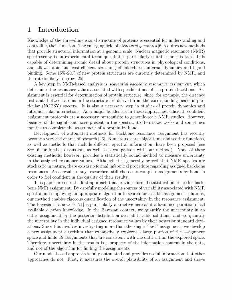
1 Introduction

Knowledge of the three-dimensional structure of proteins is essential for understanding andcontrolling their function. The emerging field of structural genomics [6] requires new methodsthat provide structural information at a genomic scale. Nuclear magnetic resonance (NMR)spectroscopy is an experimental technique that is particularly suitable for this task. It iscapable of determining atomic detail about protein structures in physiological conditions,and allows rapid and cost-efficient screening of foldedness, internal dynamics and ligandbinding. Some 15%-20% of new protein structures are currently determined by NMR, andthe rate is likely to grow [25].

A key step in NMR-based analysis is sequential backbone resonance assignment, whichdetermines the resonance values associated with specific atoms of the protein backbone. As-signment is essential for determination of protein structure, since, for example, the distancerestraints between atoms in the structure are derived from the corresponding peaks in par-ticular (NOESY) spectra. It is also a necessary step in studies of protein dynamics andintermolecular interactions. As a major bottleneck in these approaches, efficient, confidentassignment protocols are a necessary prerequisite to genomic-scale NMR studies. However,because of the significant noise present in the spectra, it often takes weeks and sometimesmonths to complete the assignment of a protein by hand.

Development of automated methods for backbone resonance assignment has recentlybecome a very active area of research [26]. Numerous search algorithms and scoring functions,as well as methods that include different spectral information, have been proposed (seeSec. 6 for further discussion, as well as a comparison with our method). None of theseexisting methods, however, provides a statistically sound method to measure uncertaintyin the assigned resonance values. Although it is generally agreed that NMR spectra arestochastic in nature, there exists no formal inferential procedure regarding assigned backboneresonances. As a result, many researchers still choose to complete assignments by hand inorder to feel confident in the quality of their results.

This paper presents the first approach that provides formal statistical inference for back-bone NMR assignment. By carefully modeling the sources of variability associated with NMRspectra and employing an appropriate algorithm to search for feasible assignment solutions,our method enables rigorous quantification of the uncertainty in the resonance assignment.The Bayesian framework [21] is particularly attractive here as it allows incorporation of allavailable a priori knowledge. In the Bayesian context, we quantify the uncertainty in anentire assignment by the posterior distribution over all feasible solutions, and we quantifythe uncertainty in the individual assigned resonance values by their posterior standard devi-ations. Since this involves investigating more than the single “best” assignment, we developa new assignment algorithm that exhaustively explores a large portion of the assignmentspace and finds all assignments that are consistent with the data within the explored space.Therefore, uncertainty in the results is a property of the information content in the data,and not of the algorithm for finding the assignments.

Our model-based approach is fully automated and provides useful information that otherapproaches do not. First, it measures the overall plausibility of an assignment and shows

(a) (b)

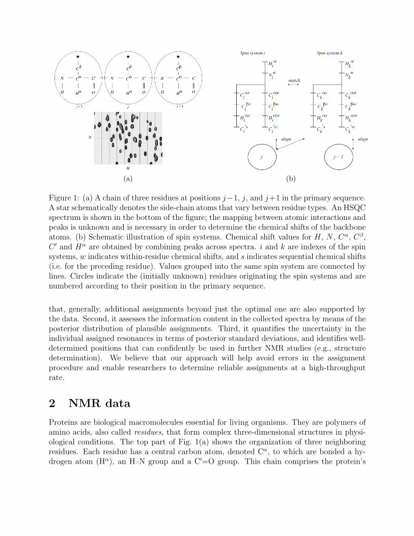
Figure 1: (a) A chain of three residues at positions j−1, j, and j+1 in the primary sequence.A star schematically denotes the side-chain atoms that vary between residue types. An HSQCspectrum is shown in the bottom of the figure; the mapping between atomic interactions andpeaks is unknown and is necessary in order to determine the chemical shifts of the backboneatoms. (b) Schematic illustration of spin systems. Chemical shift values for H, N , Cα, Cβ,C ′ and Hα are obtained by combining peaks across spectra. i and k are indexes of the spinsystems, w indicates within-residue chemical shifts, and s indicates sequential chemical shifts(i.e. for the preceding residue). Values grouped into the same spin system are connected bylines. Circles indicate the (initially unknown) residues originating the spin systems and arenumbered according to their position in the primary sequence.

that, generally, additional assignments beyond just the optimal one are also supported bythe data. Second, it assesses the information content in the collected spectra by means of theposterior distribution of plausible assignments. Third, it quantifies the uncertainty in theindividual assigned resonances in terms of posterior standard deviations, and identifies well-determined positions that can confidently be used in further NMR studies (e.g., structuredetermination). We believe that our approach will help avoid errors in the assignmentprocedure and enable researchers to determine reliable assignments at a high-throughputrate.

2 NMR data

Proteins are biological macromolecules essential for living organisms. They are polymers ofamino acids, also called residues, that form complex three-dimensional structures in physi-ological conditions. The top part of Fig. 1(a) shows the organization of three neighboringresidues. Each residue has a central carbon atom, denoted Cα, to which are bonded a hy-drogen atom (Hα), an H–N group and a C′=O group. This chain comprises the protein’s

backbone. In addition to the backbone, there are 20 different amino acid types distinguishedby the side-chain atoms attached to the Cα atoms. The side chain typically contains a carbonatom (Cβ) and other atoms schematically denoted by a star in Fig. 1(a). Two exceptions areproline, which replaces H and Hα with a cycle of atoms from the N to the Cα, and glycine,which has another Hα instead of a Cβ. The number and order of amino acid types in aprotein — its primary sequence — is determined by other experimental techniques prior tostudy by NMR.

NMR spectroscopy [8] takes advantage of the magnetic properties of atomic nuclei. Whena protein sample is placed into a static magnetic field and exposed to another oscillating mag-netic field, the individual nuclei respond at specific resonance frequencies. These resonancefrequencies, or chemical shifts, are very sensitive to the chemical environment surrounding anucleus and are thus in principle unique for each atom in a typical moderate-sized globularprotein. Chemical shifts are central to NMR-based studies, as they provide the “IDs” of theatoms, by which the atoms can be referenced in subsequent studies of structure, dynamics,and interactions. The goal of backbone resonance assignment is to determine the chemicalshift values for the nuclei in the protein backbone.

Backbone resonance assignment employs data from a set of NMR experiments. A centralexperiment is the HSQC, which magnetically correlates bonded H–N nuclei and yields a two-dimensional spectrum. An example fragment of an HSQC spectrum is shown in the bottomof Fig. 1(a). Peaks in the spectrum indicate H–N bonded pairs at specific chemical shifts(their coordinates). The HSQC is a core experiment since each residue except proline has anH–N pair and thus (in ideal conditions) generates such a peak. However, the correspondencebetween the peak and the H–N pair that generated it is unknown.

Determination of the chemical shifts of the atoms in the backbone also requires at leastone, and usually several, three-dimensional NMR experiments. An example of such anexperiment is the HNcoCA, which magnetically correlates bonded H–N backbone nuclei withthe Cα nucleus of the preceding residue. The experiment yields a three-dimensional spectrum,in which the projection on the H–N dimensions corresponds to the HSQC, and the thirddimension to the magnetically correlated Cα. Since each HNcoCA peak correlates atomsin two neighboring residues, the experiment is useful in identifying sequential interactions.Another three-dimensional experiment, the HNCA, correlates the bonded H–N pairs withthe Cα of either the preceding residue (as in the HNcoCA) or of the same residue. Ityields approximately twice as many three-dimensional peaks as the HNcoCA, gatheringboth sequential and within-residue interactions. Similar NMR experiments can be designedto involve interactions of the H–N pairs with Cβ, Hα, and C′. The type of atoms involvedin a spectrum is called its resonance type. Again, it is important to note that the residue(s)whose atoms generated each peak is initially unknown for all spectra.

The chemical shifts can be determined by finding a mapping between the peaks and theatoms. In summary, a typical procedure to find such a mapping consists of the followingsteps [26, 33]: (1) identify and determine the centers of peaks within the spectra; (2) groupthe peaks into collections called spin systems according to their shared H–N resonances;(3) match spin systems according to corresponding sequential and within-residue chemical

shifts; (4) align connected chains of spin systems to the primary sequence according to theexpected chemical shifts for corresponding residue types. We now detail each step in thisprocedure.

Peak analysis. Peaks in NMR spectra do not have precise positions. As illustrated inthe HSQC in Fig. 1(a), they span some volume, shown in the figure by intensity contours.The volume of a peak depends on the physical properties of the nucleus, as well as the typeand sensitivity of the NMR experiment. The coordinates of the center of a peak can bedetermined by automated peak picking software such as NMRDraw [10]. The center canbe determined fairly accurately for a well-resolved peak, but the accuracy is compromisedwhen the peak is broad or has a low intensity, or when several peaks overlap. Peak positionsare also subject to random variation between spectra, due to sample variation, differencesin sample temperature and other experimental artifacts. In summary, the coordinates of thecenters of the peaks can be viewed as noisy readings from the underlying chemical shifts,having a compound variation from within and between the spectra.

Peak picking software produces a list of peaks, which typically is missing some peaksand has some extra (spurious) peaks. Peaks can be missing due to physical reasons (e.g. anoverly broad peak resulting from extensive dynamics), spectral degeneracy (e.g. peaks tooclose together to be differentiated), or noise. Spurious peaks can originate from impuritiesin the sample, minor conformations of the protein, or errors in the peak picking procedure.

Compilation of spin systems. The spectra we employ here all involve the “anchor”H–N pairs. Thus one can combine peaks across spectra by referencing the H–N coordinates.The third coordinate is classified according to resonance type as shown in Fig. 1(b). Thesecollections of peaks, called spin systems, typically consist of within-residue and sequentialchemical shifts of several resonance types, anchored at one (unknown) residue and connectingto its predecessor. Due to the noise in peaks discussed above, some spin systems can havemissing chemical shift values, some spin systems can be entirely missing, and some extra,spurious spin systems can be compiled from extra, spurious peaks. Due to variability in peakpositions, approximate equality of peak coordinates must be allowed when compiling spinsystems. While the compilation is unambiguous for isolated peaks, ambiguities can arise inthe case of close or overlapping peaks.

Matching spin systems. Spin systems can be arranged into ordered chains by matchingthe sequential resonances of one with the within-residue resonances of another. If two spinsystems originate from the neighboring residues as shown in Fig. 1(b), the within-residuechemical shifts of the first spin system must be approximately the same as the sequentialchemical shifts of the following spin system. Approximate matches must be allowed due tonoise, and ambiguities arise when several spin systems have similar sequential or within-residue values. The number of plausible matches increases dramatically when the datacontains a large number of missing resonance types or entirely missing spin systems —the missing chemical shifts become “wild cards” that allow matches to any spin system.Extra spin systems result in additional complications as they are often incomplete, and cansometimes form an incorrectly unambiguous match.

Aligning spin systems. Spin systems can be aligned to positions in the primary

sequence by comparing chemical shifts to the values expected for the corresponding residuetypes. Since an atom’s chemical shift is sensitive to its local chemical environment, there isa well-characterized effect of amino acid type on chemical shift. The expected ranges canbe determined from databases such as BioMagResBank [29] or RefDB [34], which containassignments for many proteins. Unfortunately, the ranges are typically quite broad, andallow a spin system to align to any of many possible positions in the primary sequence.Chains of connected spin systems are required in order to overcome this ambiguity, whereeach spin system agrees that the corresponding position is consistent. However, even shortchains of spin systems can typically be aligned at several places in the sequence. We notetwo special cases in alignment: given the H–N based spin system definition here, alignmentsare not possible at the first residue or proline residues; further, alignments are restricted atglycine residues due to the substitution of an extra Hα for the Cβ.

This paper assumes that the data have been correctly processed and the spin systemscompiled by either manual or automated methods. We focus on the problem of matchingsequentially-connected spin systems and aligning them to the primary sequence. For clarity,we make a distinction between the result of matching and aligning spin systems to thesequence, which we call a “mapping,” and the determination of the unknown resonancevalues on the basis of a mapping. We use “assignment” to denote the entire procedure.

A mapping is established by systematically matching and aligning the spin systems, muchlike a jigsaw puzzle. Each spin system can have at most one predecessor and can be mappedto at most one spin system, and each position can be mapped to at most one spin system.Positions with no mapped spin systems are associated with entirely missing spin systems,and spin systems not mapped to positions are considered extras. Satisfactory mappingscover the maximum number of positions. In principle, there exists one “correct” mappingthat generated the data. In practice, however, the large number of ambiguities at each stepof the procedure often results in several plausible mappings that need to be considered. Asdiscussed in the introduction, our method enumerates all plausible mappings and uses theirposterior distribution in a model-based approach to quantify the uncertainty.

The goal of backbone resonance assignment is to determine the chemical shifts of theprotein backbone. A mapping between the spin systems and positions in the sequence is ameans to this end. Given a mapping, the chemical shifts of a nucleus can be deduced fromthe associated peaks. However, uncertainty in the peak positions and uncertainty in themappings result in uncertainty in chemical shifts.

3 Methods

We view backbone resonance assignment as a process of estimating the chemical shifts ofthe protein backbone from noisy data. A candidate mapping, combined with distributionalassumptions regarding the peaks, can then be viewed as a statistical model of the data.From this perspective, the search for the “best” candidate mapping becomes a model se-lection problem. When several models are plausible, inference about the unknowns shouldincorporate both the uncertainty in the data and the uncertainty in the model selection.

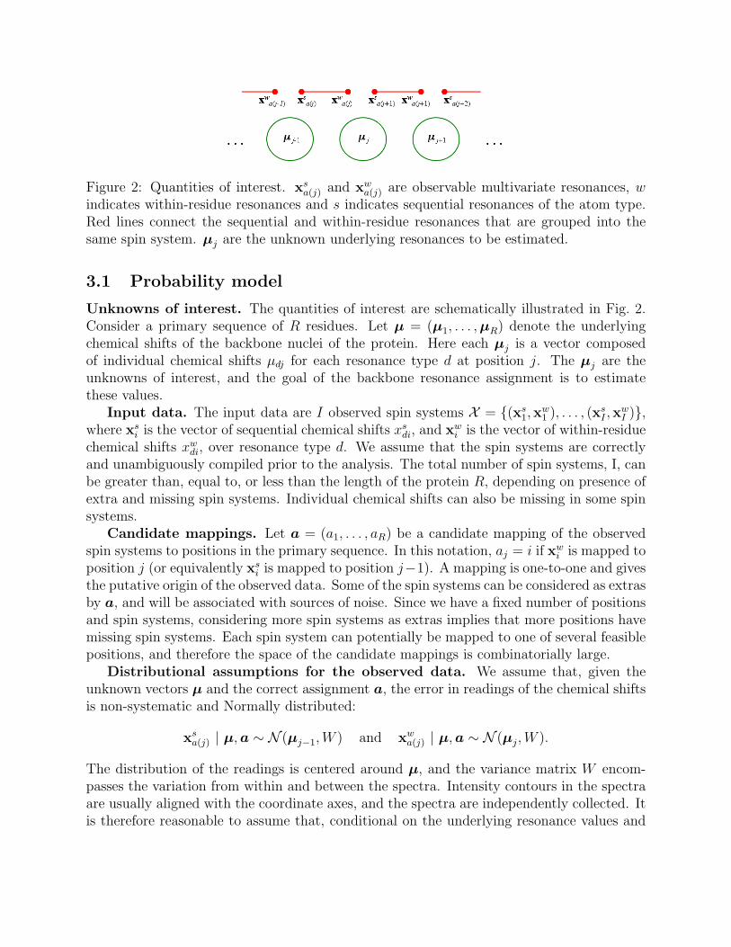
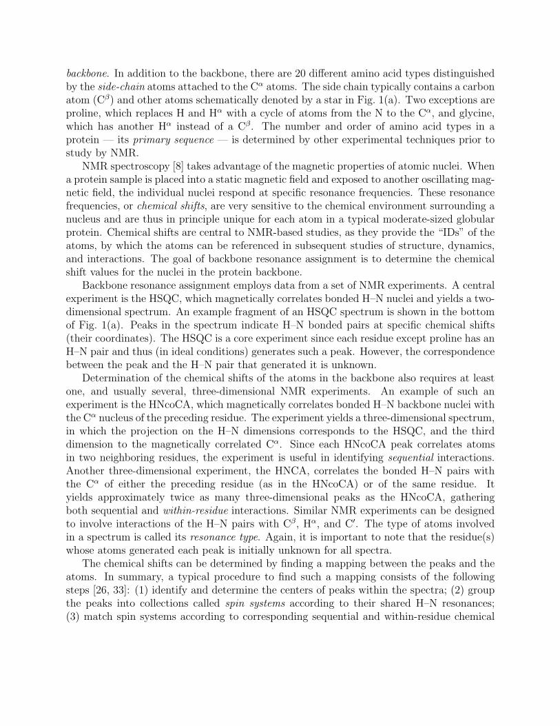
Figure 2: Quantities of interest. xsa(j) and xw

a(j) are observable multivariate resonances, windicates within-residue resonances and s indicates sequential resonances of the atom type.Red lines connect the sequential and within-residue resonances that are grouped into thesame spin system. µj are the unknown underlying resonances to be estimated.

3.1 Probability model

Unknowns of interest. The quantities of interest are schematically illustrated in Fig. 2.Consider a primary sequence of R residues. Let µ = (µ1, . . . ,µR) denote the underlyingchemical shifts of the backbone nuclei of the protein. Here each µj is a vector composedof individual chemical shifts µdj for each resonance type d at position j. The µj are theunknowns of interest, and the goal of the backbone resonance assignment is to estimatethese values.

Input data. The input data are I observed spin systems X = {(xs1,x

w1 ), . . . , (xs

I ,xwI )},

where xsi is the vector of sequential chemical shifts xs

di, and xwi is the vector of within-residue

chemical shifts xwdi, over resonance type d. We assume that the spin systems are correctly

and unambiguously compiled prior to the analysis. The total number of spin systems, I, canbe greater than, equal to, or less than the length of the protein R, depending on presence ofextra and missing spin systems. Individual chemical shifts can also be missing in some spinsystems.

Candidate mappings. Let a = (a1, . . . , aR) be a candidate mapping of the observedspin systems to positions in the primary sequence. In this notation, aj = i if xw

i is mapped toposition j (or equivalently xs

i is mapped to position j−1). A mapping is one-to-one and givesthe putative origin of the observed data. Some of the spin systems can be considered as extrasby a, and will be associated with sources of noise. Since we have a fixed number of positionsand spin systems, considering more spin systems as extras implies that more positions havemissing spin systems. Each spin system can potentially be mapped to one of several feasiblepositions, and therefore the space of the candidate mappings is combinatorially large.

Distributional assumptions for the observed data. We assume that, given theunknown vectors µ and the correct assignment a, the error in readings of the chemical shiftsis non-systematic and Normally distributed:

xsa(j) | µ, a ∼ N (µj−1, W ) and xw

a(j) | µ, a ∼ N (µj, W ).

The distribution of the readings is centered around µ, and the variance matrix W encom-passes the variation from within and between the spectra. Intensity contours in the spectraare usually aligned with the coordinate axes, and the spectra are independently collected. Itis therefore reasonable to assume that, conditional on the underlying resonance values and

assignment, the readings are independent between the resonance types. This implies thatW is a diagonal matrix.

We further assume that, conditional on µ and a, the readings from the chemical shifts areindependent across positions in the sequence. Note that the independence is conditional andwill not hold marginally across all the candidate mappings. The assumption may oversimplifythe correlation structure in the data since peaks collected within a single spectrum may co-vary. On the other hand, as discussed in Sec. 6, independence across positions is implicitlyassumed by all existing automated methods for backbone resonance assignment.

Finally, we assume that the variance matrix W is known and constant for all xsa(j) and

xwa(j). Weaknesses of this assumption include the possibility that peaks within a spectrum

may have different resolutions, and the fact that the chemical shifts in a spin system summa-rize various numbers of peaks. However, estimation of the spin system-specific variances is adifficult task, requiring grouping of all peaks according to their common (unknown) source,and given that only one peak per source is available in many cases. As discussed in Sec. 6,constant and known variance is implicitly assumed by most current automated methods, andsome generally accepted variance values are typically used. We follow this approach here,but plan to investigate the problem of spin system-specific variances in our future work.

Given the distributional assumptions above, the conditional likelihood of the compositeof the positions in the primary sequence can be written as

Pr(x | µ, a) =R∏

j=1φ

(W− 1

2 (xsa(j) − µj−1)

)φ

(W− 1

2 (xwa(j) − µj)

).

Here and in the rest of the paper φ denotes the density of the multivariate standard Normaldistribution.

Prior distributions of the unknown µ. The distributions of chemical shifts of previ-ously assigned proteins, as deposited in various databases, can be used to characterize the µj

a priori. We assume that the µj are independent across all positions in the primary sequenceand Normally distributed, i.e. µj ∼ N (θj, Σj). The vector θj contains mean chemical shiftsof all resonance types, and Σj is the corresponding variance-covariance matrix estimatedfrom the database. The parameters θj and Σj are specific to the residue type at the positionj.

Both θj and Σj can be estimated from at least two databases, the BioMagResBank [29]and the RefDB [34], and in a number of ways. For example, one can assume that theresonance types are a priori independent, in which case Σj is a diagonal matrix, and takethe database means and variances as the parameter estimates. Alternatively, one can assumea non-diagonal Σj and compute the correlation between the resonance types [24]. A moresophisticated approach would account for the redundancy in the sequences deposited into theBioMagResBank, and estimate the parameters from the subset of non-homologous sequencesonly [24, 31]. Or, when the information on the secondary structure of the protein is available,one can account for systematic effects of secondary structure type on chemical shift [32]. Allof these methods are equally well supported by our approach, and Normal distributions withany parameters can be used provided that they are appropriately justified. In Sec. 5.2 we

conduct a sensitivity analysis and investigate the extent to which the choice of the parametersof the prior distributions affects the inference of the unknowns µ.

One may question the choice of the Normal prior distribution. Although the Normalityassumption can in principle be substituted by any other distribution of choice, the Normaldistribution is particularly attractive as it allows the analytical computation of posteriorprobabilities, and is therefore computationally efficient. The Normal distribution providesan adequate approximation of the chemical shifts in most cases and, as discussed in Sec. 6,is implicitly used by many existing methods of backbone resonance assignment. Some dis-tributions in the databases may appear to have heavier than Normal tails. In this case,a spin system with outlying chemical shifts will not be correctly mapped to the primarysequence, and the corresponding position in the sequence will be associated with a missingspin system. An alternative solution is to increase the variance of the prior distribution inorder to accommodate the tails.

Sources of noise. For completeness, we assume that the extra spin systems are readingsfrom the underlying chemical shifts (µR+1, µR+2, . . .) of the sources of noise. We specify anon-informative Normal prior for the parameters by choosing θj, j > R, to be the mid-rangeof the measurements of each resonance type, and Σj, j > R, to cover the entire measurementrange.

3.2 Scoring the candidate mappings

The probability model allows us to compare and evaluate the candidate mappings in termsof their posterior probabilities given the data. These can be obtained by applying Bayestheorem, and by averaging across the unknown parameters µ [27]

Pr(a|x) ∝ Pr(x|a)Pr(a), where Pr(x|a) =∫

Pr(x|µ, a)Pr(µ)dµ. (1)

As can be seen, the posterior probability Pr(a|x) in (1) consists of two terms: the likelihoodPr(x|a), and the prior distribution Pr(a) of a mapping a.

Likelihood. The conjugate Normal structure of our model makes it possible to carryout the integration in (1) analytically. Upon integration, the likelihood can be written as

Pr(x|a) =R∏

j=1φ

(U

− 12

1 (xsa(j+1) − xw

a(j)))

φ(

U− 1

22 (xa(j) − θj)

), (2)

where xa(j) is the average of xsa(j+1) and xw

a(j), U1∆= 2W and U2

∆= Σj + W/2. The ob-

servations mapped to a position j in the primary sequence contribute to the likelihood viatwo terms. The first involves the quantity xs

a(j+1) − xwa(j) and reflects the likelihood of the

sequential connectivity at this position. The second involves the quantity xa(j) and reflectsthe consistency of the chemical shifts with the expectations of the mapped amino acid type.Because of the non-informative prior distribution of the sources of noise, their contributionto the likelihood is approximately 1, and can be ignored.

When comparing candidate mappings, it is helpful to consider S(x|a) = −2 log Pr(x|a),which can be viewed as a score measuring the success of a at predicting the data. In ourcase,

S(x|a) =R∑

j=1

Smatch, j +R∑

j=1

Salign, j (3)

whereSmatch, j = (xs

a(j+1) − xwa(j))

′(2W )−1(xsa(j+1) − xw

a(j))

Salign, j = (xa(j) − θj)′(Σj + W/2)−1(xa(j) − θj).

Maximizing the likelihood is equivalent to minimizing the score. Under the assumptions inSec. 3.1 and given the correct assignment a, S(x|a) follows the χ2

df distribution. Moreover,a partial score computed over any subset of positions in the sequence also follows the χ2

df .The integer df in this notation is the number of chemical shifts, xs

di and xwdi, used to compute

the specific score. Although not part of the formal Bayesian framework, this interpretationis very useful as only those mappings that are consistent with the distribution need to beconsidered [28]. In practice, we can compare the scores with an α-quantile of the χ2

df fora (small) pre-specified probability α, and reject the mappings with scores exceeding thequantile.

Prior distribution of the candidate mappings. A complete mapping is preferableto one with many missing observations. For example, a mapping considering most of theobserved spin systems as noise is likely to be false. On the other hand, a spin system wheremost chemical shifts are missing is likely to be an extra. We therefore penalize the candidatemappings according to the number of missing chemical shifts associated with the positionsin the sequence. Specifically, we define the prior probability of a mapping with d missingresonances as

Pr(a) ∝ exp {−12qχ2(α, df)} (4)

where qχ2(α, df) denotes the α-quantile of the χ2 distribution with df degrees of freedom. Onthe −2 log scale, the prior amounts to substituting a worst-case estimate for the contributionto the posterior probability of a missing observation.

The mappings with the highest posterior probabilities are used for inference about theunknown µ. Therefore, a candidate mapping can be discarded if its fit to the data is clearlyworse than that of the best mapping found [16, 17]. In the following definition, we combinethe interpretations on the scale of the posterior probability and on the scale of the scorefunction.

Definition 1 (Mapping Consistency) A mapping a is consistent with the data if, for agiven (small) probability α,

1. Smatch, j < qχ2(α, dfmatch, j) for all j.

2. Salign, j < qχ2(α, dfalign, j) for all j.

3. Smatch, j + Salign, j < qχ2(α, dfmatch, j + dfalign, j) for all j.

4. S(x|a) < qχ2(α, df).

5. P (x|a∗)/P (x|a) ≤ 25 where a∗ is the mapping with the highest posterior probability.

df in the definition denotes the number of data points used to compute the correspondingscore. Note that Smatch, j and Salign, j represent the joint score of all resonance types ofinterest at position j. Therefore, a relatively loose match or alignment of one resonance typeis considered as plausible if it is compensated for by a relatively strong match or alignmentof the other resonance types. Although one can also define consistency separately for eachresonance type, we found that in practice this definition provides more flexibility and resultsin more accurate assignments. The parameter α flexibly determines the search space ofcandidate mappings. Smaller α values result in more mappings being considered plausible,and the larger values result in rejection of more mappings.

3.3 Inference

Inference regarding µ can be made by means of its posterior distribution given the data. Ifonly one mapping a is consistent with the data as in Definition 1, it can be used as the basisfor inference [27]

µdj | x, a ∼ N (xd a(j), wd/2). (5)

where µdj is the unknown chemical shift of resonance type d at position j, xd a(j) is the dthelement of the average of xs

a(j+1) and xwa(j), and wd is the dth diagonal element of W . Since

the experimental variance is orders of magnitude smaller than the variance of the prior of µ,the contribution of the prior of µj to (5) can be ignored. When K mappings are consistentwith the data, inference based on the mapping with the highest posterior probability willunderestimate the uncertainty in the correct mapping, as well as the differences in µj underthe other reasonably good alternatives. This uncertainty can be taken into account byaveraging the posterior distribution of µj across all candidate mappings [16, 17]

Pr(µj|x) =K∑

k=1Pr(µj|x, ak)Pr(ak|x) (6)

where Pr(ak|x) are standardized to form a probability distribution on the set of the selectedmappings. The µdj can be estimated by their posterior means, and the quality of estimationcan be characterized by their posterior standard deviations:

E(µdj|x) =K∑

k=1xd ak(j)Pr(ak|x) and

Var(µdj|x) =K∑

k=1(wd/2 + x2

d ak(j))Pr(ak|x)− x2d ak(j) ,

The posterior mean of µj is nothing but a weighted average of estimations according tothe individual mappings. Therefore, if a spin system is mapped to the same position in all

mappings, the posterior standard deviation equals the standard deviation of the readingsof the peak positions. If different spin systems are mapped to a position, the posteriordeviation of µ at this position incorporates both the uncertainty in the spin system andthe experimental variance. The possibility of mapping different spin systems to a positiondoes not necessarily imply uncertainty in the chemical shifts. Some alternative spin systemsmay have similar values in all or at least some resonance types, in which case the posteriorstandard deviation will remain close to the experimental precision. Alternatively, if therelative weight of a candidate mapping is small, the contribution of the mapping will notsignificantly inflate the posterior standard deviation.

In addition to the inference of µ, it is instructive to examine the posterior distributionPr(ak|x) for the set of candidate mappings. The shape of the distribution can be used tocharacterize the information content in the data: the sharper the distribution, the moreevidence there is in favor of the mapping with the highest posterior probability. One shouldnot, however, confuse the inference regarding a with the inference regarding µ. As discussedin the previous paragraph, uncertainty in the candidate mappings may or may not result inuncertainty in the estimated chemical shifts.

The posterior distribution Pr(ak|x) provides a relative measure of quality for one mappingwith respect to another. But it does not provide the information on how well the mapping fitsthe data. The scores of the candidate mappings, on the other hand, measure the goodness offit. One can compare the scores with the α-quantiles of the corresponding χ2

df distributionsin order to judge the overall plausibility of the selected mappings.

4 Finding plausible candidate mappings

The proposed inferential procedure can be carried out using any algorithm which appro-priately explores the probability space of candidate mappings and finds the mappings withthe highest posterior probabilities. A limited number of mappings is expected to satisfy theconditions in Definition 1. Therefore, an exhaustive search is the most desirable procedureas it ensures complete examination of the search space and does not omit any mapping ofinterest. It has a particular advantage over greedy and best-first algorithms favoring locallyoptimal choices, which may not necessarily lead to overall plausible solutions and may ignorechoices that do. Several exhaustive search algorithms for backbone resonance assignmenthave recently appeared in the literature and demonstrated the feasibility of this approachfor problems of moderate size [1, 9, 20, 31]. However, the algorithms are based on scoringfunctions with no probability interpretation. We require an algorithm capable of exploringthe probability space of candidate mappings and providing all solutions consistent with thedata.

We illustrate our inferential procedure using a new algorithm of this kind. Our proba-bility model provides information not available to the previous algorithms mentioned above.Specifically, we can evaluate the partial scores of matching and aligning any groups of spinsystems with any portions of the primary sequence. In addition, the χ2 interpretation ofthe scores provides an upper bound for the score of the correct mapping. Finally, the search

space can be characterized in terms of the probability of missing the mapping that generatedthe data. Thus we can prune the search space in a statistically sound manner, discardingfrom further consideration partial solutions not worth completing.

The probability model allows our algorithm to handle larger spaces of candidate mappingsthan what has been previously found tractable. In particular, it provides a general, consistenttreatment of entirely missing spin systems. Previous algorithms only consider a missing spinsystem when no other matching can be found. This results in an arbitrary unequal treatmentof the spin systems, as a plausible match can sometimes be successfully substituted by amatch with a missing spin system. We propose an algorithm which handles all positions andall spin systems in a symmetric way. It examines the possibility of a missing spin systemat any position in the sequence, and limits the search space only by a maximum allowablenumber of missing spin systems. A penalty (Eq. 4) discourages mappings with many missingchemical shifts, and therefore entirely missing spin systems will not appear at every positionin the sequence. For most positions for which there are possible spin systems, the scores ofmatching and aligning are better than the corresponding penalty, and therefore a missingspin system will not appear plausible. Our current approach looks for candidate mappingswith the smallest number of entirely missing spin systems; a careful choice of the maximumnumber of missing spin systems will be the subject of future work.

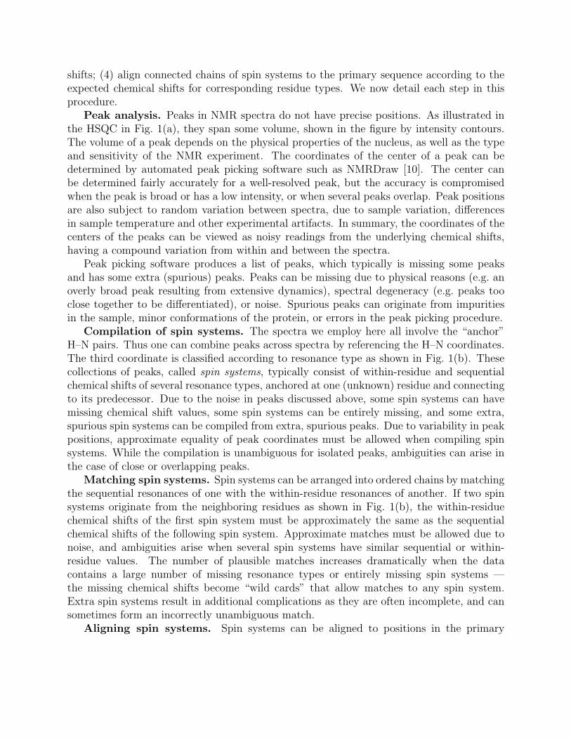
The algorithm is summarized in Fig. 3 and Fig. 4, and illustrated in Fig. 5. Ratherthan performing a combinatorial enumeration of individual spin systems and positions inthe primary sequence as is typically done, our algorithm works at a coarser grain: it usesconnected spin systems (which we call strands), and subsequences of the primary sequence(windows). It starts with an initialization step (Fig. 3(I) and Fig. 5(a)) that maps eachobserved spin system to each position in the sequence, subject to restrictions described inSec. 2. A placeholder representing an entirely missing spin system is also mapped to eachposition. The next step (Fig. 3(II) and Fig. 5(b)) of the algorithm sets up the coarser-grained data structures for the search. It grows windows with strands sequentially startingfrom the first position. Specifically, the step starts by examining all possible strands that canbe mapped to the first two positions, then proceeds by examining the strands that can bemapped to the first three positions, and so forth moving sequentially towards the end of theprotein. Since the number of strands grows combinatorially with the number of positionsexamined, an execution parameter controls the maximum number of strands that can bemapped to a same set of positions. Every time the number of strands reaches the limit, thegrowth of the current window is stopped, and a new set of strands and a new window arestarted from the following position. Therefore, by design, the windows do not overlap andthe number of strands in the windows is approximately equal and never exceeds the specifiedlimit.

Not all the strands constructed during step II are kept at the end of this step. Forexample, a strand that is guaranteed to produce a poor score in combination with anyother strand from the remaining windows (called “outer strands” in the pseudocode) canbe discarded. Similarly, one can discard a strand which, in combination with other strands,will exceed the pre-specified limit on number of missing spin systems. Furthermore, the step

introduces a parameter β which provides an additional constraint on evaluation of partialmappings. Specifically, if the score of a strand exceeds the β-quantile of the correspondingχ2 distribution, the strand is rejected. These criteria for a valid merge are summarized inFig. 4.

The step II reduces the search space of candidate mappings. The last stage of thealgorithm (Fig. 3(III)) performs an exhaustive depth-first search of the reduced space bymerging the strands in the windows. This can be done sequentially starting from the firstwindow, but a careful choice of the order of merging can greatly improve the execution time.

The parameter α in Definition 1 and β in Step II jointly limit the search space of candidatemappings. By using the conservative Bonferroni correction to multiple comparisons [15], theprobability of rejecting the correct mapping for at least one position is at most (3R + 1)α +2Rβ. Therefore, α and β can be chosen to control the familywise error rate at the desiredlevel. Alternatively, one can undertake a more aggressive approach and choose α and βto control the False Discovery Rate (i.e. the expected proportion of positions at which thecorrect mapping is rejected) [5]. We believe that in this problem, the Bonferroni correctionis superior to the FDR-controlling approach for two reasons. First, it is desirable to makeas few incorrect rejections as possible at all positions in the sequence, and the familywiseBonferroni correction is an appropriate metric for that. Second, the Bonferroni correction iscomputationally inexpensive and results in a larger space of candidate mappings. Therefore,computational effort is used to explore alternative mappings rather than to calculate theFDR-based rejection thresholds.

5 Results

5.1 Data example

We illustrate our inferential procedure for resonance assignment in application to two pro-teins, Human Ubiquitin and the single-stranded DNA-binding cold-shock protein A (CspA)from Escherichia coli. Human Ubiquitin is a 76 amino acid residue protein used as a bench-mark in many NMR studies. The data set containing peaks from 7 through-bond experi-ments and providing connectivity information for Cα, Cβ and C′ resonance types is publiclyavailable from the Ubiquitin NMR Resource Web Page [30]. We manually compiled thespin systems from the observed peaks. Two expected spin systems were missing, and noextra spin systems were detected. The correct mapping of the spin systems to positions inthe sequence is the one deposited in the database, and we will refer to it as the referencemapping.

The single-stranded DNA-binding cold-shock protein A (CspA) from Escherichia coli isa small β-sheet protein composed of 70 residues. NMR data are provided as a test for theAutoAssign program [35], and include peak lists from eight through-bond NMR experimentsyielding connectivity information for Cα, Cβ, and Hα. One of the experiments involves theC′ resonance type. AutoAssign compiles the resonance peaks into spin systems and findsassignments for all non-proline residues except for the first two. In addition, AutoAssign

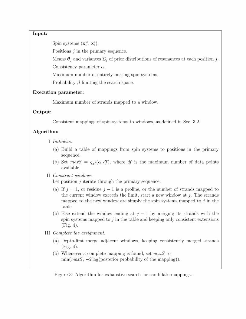
Input:

Spin systems (xwi , xs

i ).

Positions j in the primary sequence.

Means θj and variances Σj of prior distributions of resonances at each position j.

Consistency parameter α.

Maximum number of entirely missing spin systems.

Probability β limiting the search space.

Execution parameter:

Maximum number of strands mapped to a window.

Output:

Consistent mappings of spin systems to windows, as defined in Sec. 3.2.

Algorithm:

I Initialize.

(a) Build a table of mappings from spin systems to positions in the primarysequence.

(b) Set maxS = qχ2(α, df), where df is the maximum number of data pointsavailable.

II Construct windows.Let position j iterate through the primary sequence:

(a) If j = 1, or residue j − 1 is a proline, or the number of strands mapped tothe current window exceeds the limit, start a new window at j. The strandsmapped to the new window are simply the spin systems mapped to j in thetable.

(b) Else extend the window ending at j − 1 by merging its strands with thespin systems mapped to j in the table and keeping only consistent extensions(Fig. 4).

III Complete the assignment.

(a) Depth-first merge adjacent windows, keeping consistently merged strands(Fig. 4).

(b) Whenever a complete mapping is found, set maxS tomin(maxS , −2 log(posterior probability of the mapping)).

Figure 3: Algorithm for exhaustive search for candidate mappings.

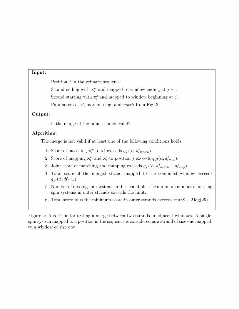
Input:

Position j in the primary sequence.

Strand ending with xwi and mapped to window ending at j − 1.

Strand starting with xsi and mapped to window beginning at j.

Parameters α, β, max missing, and maxS from Fig. 3.

Output:

Is the merge of the input strands valid?

Algorithm:

The merge is not valid if at least one of the following conditions holds:

1. Score of matching xwi to xs

i exceeds qχ2(α, dfmatch).

2. Score of mapping xwi and xs

i to position j exceeds qχ2(α, dfmap).

3. Joint score of matching and mapping exceeds qχ2(α, dfmatch + dfmap).

4. Total score of the merged strand mapped to the combined window exceedsqχ2(β, dftotal).

5. Number of missing spin systems in the strand plus the minimum number of missingspin systems in outer strands exceeds the limit.

6. Total score plus the minimum score in outer strands exceeds maxS + 2 log(25).

Figure 4: Algorithm for testing a merge between two strands in adjacent windows. A singlespin system mapped to a position in the sequence is considered as a strand of size one mappedto a window of size one.

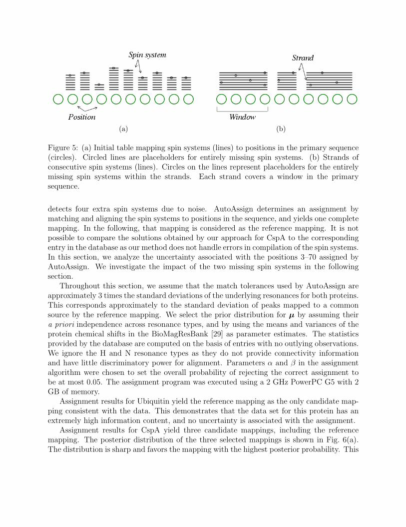
(a) (b)

Figure 5: (a) Initial table mapping spin systems (lines) to positions in the primary sequence(circles). Circled lines are placeholders for entirely missing spin systems. (b) Strands ofconsecutive spin systems (lines). Circles on the lines represent placeholders for the entirelymissing spin systems within the strands. Each strand covers a window in the primarysequence.

detects four extra spin systems due to noise. AutoAssign determines an assignment bymatching and aligning the spin systems to positions in the sequence, and yields one completemapping. In the following, that mapping is considered as the reference mapping. It is notpossible to compare the solutions obtained by our approach for CspA to the correspondingentry in the database as our method does not handle errors in compilation of the spin systems.In this section, we analyze the uncertainty associated with the positions 3–70 assigned byAutoAssign. We investigate the impact of the two missing spin systems in the followingsection.

Throughout this section, we assume that the match tolerances used by AutoAssign areapproximately 3 times the standard deviations of the underlying resonances for both proteins.This corresponds approximately to the standard deviation of peaks mapped to a commonsource by the reference mapping. We select the prior distribution for µ by assuming theira priori independence across resonance types, and by using the means and variances of theprotein chemical shifts in the BioMagResBank [29] as parameter estimates. The statisticsprovided by the database are computed on the basis of entries with no outlying observations.We ignore the H and N resonance types as they do not provide connectivity informationand have little discriminatory power for alignment. Parameters α and β in the assignmentalgorithm were chosen to set the overall probability of rejecting the correct assignment tobe at most 0.05. The assignment program was executed using a 2 GHz PowerPC G5 with 2GB of memory.

Assignment results for Ubiquitin yield the reference mapping as the only candidate map-ping consistent with the data. This demonstrates that the data set for this protein has anextremely high information content, and no uncertainty is associated with the assignment.

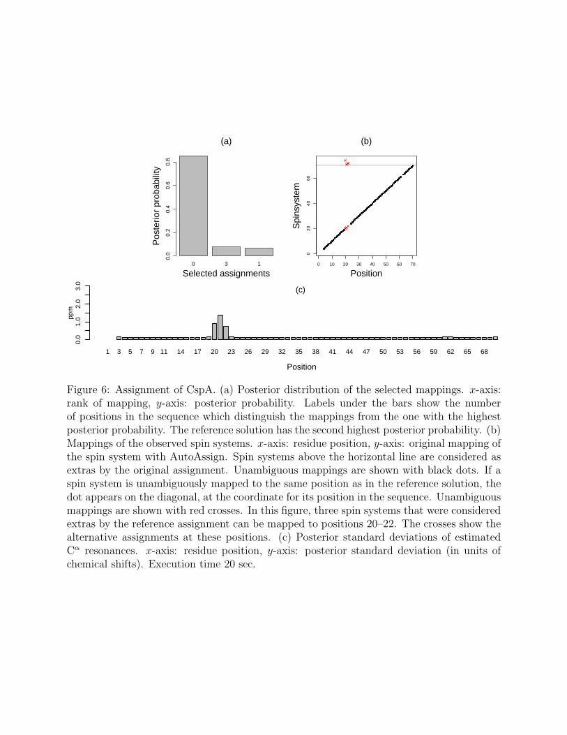
Assignment results for CspA yield three candidate mappings, including the referencemapping. The posterior distribution of the three selected mappings is shown in Fig. 6(a).The distribution is sharp and favors the mapping with the highest posterior probability. This

0 3 1

0.0

0.2

0.4

0.6

0.8

Selected assignments

Pos

terio

r pr

obab

ility

(a)

0 10 20 30 40 50 60 70

020

4060

Position

Spi

nsys

tem

(b)

1 3 5 7 9 11 14 17 20 23 26 29 32 35 38 41 44 47 50 53 56 59 62 65 68

0.0

1.0

2.0

3.0

(c)

ppm

Position

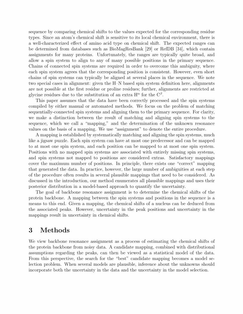
Figure 6: Assignment of CspA. (a) Posterior distribution of the selected mappings. x-axis:rank of mapping, y-axis: posterior probability. Labels under the bars show the numberof positions in the sequence which distinguish the mappings from the one with the highestposterior probability. The reference solution has the second highest posterior probability. (b)Mappings of the observed spin systems. x-axis: residue position, y-axis: original mapping ofthe spin system with AutoAssign. Spin systems above the horizontal line are considered asextras by the original assignment. Unambiguous mappings are shown with black dots. If aspin system is unambiguously mapped to the same position as in the reference solution, thedot appears on the diagonal, at the coordinate for its position in the sequence. Unambiguousmappings are shown with red crosses. In this figure, three spin systems that were consideredextras by the reference assignment can be mapped to positions 20–22. The crosses show thealternative assignments at these positions. (c) Posterior standard deviations of estimatedCα resonances. x-axis: residue position, y-axis: posterior standard deviation (in units ofchemical shifts). Execution time 20 sec.

indicates high information content in the data. The candidates are overall plausible withp-values of the corresponding score functions greater than 0.9. The reference mapping hasthe second largest posterior probability, but the largest number of non-missing resonances.Since the original mapping was obtained using a different scoring function, we do not expectit to be the most likely a posteriori. Most spin systems are uniquely mapped to positionsin the primary sequence, and the selected mappings differ in at most 3 positions. Fig. 6(b)details the alternative mappings. The alternatives are due to plausible mappings of extra spinsystems to positions 20–22. The posterior standard deviations of the estimated resonancevalues for the Cα resonance type are shown in Fig. 6(c). The posterior standard deviationsat the unambiguous positions are equal to the assumed experimental precision. However,the posterior standard deviations at positions 20–22 are high, indicating uncertainty in thisregion. This ability to uncover uncertainty is a key advantage of our approach over traditionaloptimization-based approaches which provide only a single best mapping.

5.2 Simulation study

In order to demonstrate the importance of inference for resonance assignment, we investi-gated the impact of the choices of experimental design and non-systematic sources of noise.In the following, we systematically perturb the observed spin systems of CspA and studythe effect of these modifications on the assignment.

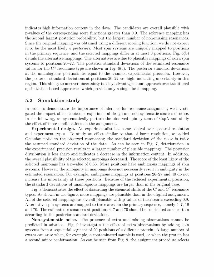
Experimental design. An experimentalist has some control over spectral resolutionand experiment types. To study an effect similar to that of lower resolution, we addedGaussian noise to the observed resonances; the standard deviation of the noise is twicethe assumed standard deviation of the data. As can be seen in Fig. 7, deterioration inthe experimental precision results in a larger number of plausible mappings. The posteriordistribution is less sharp and indicates a decrease in the information content. In addition,the overall plausibility of the selected mappings decreased. The score of the least likely of theselected mappings has a p-value of 0.53. More positions have ambiguous mappings of spinsystems. However, the ambiguity in mappings does not necessarily result in ambiguity in theestimated resonances. For example, ambiguous mappings at positions 26–27 and 40 do notincrease the uncertainty at these positions. Because of the reduced experimental precision,the standard deviations of unambiguous mappings are larger than in the original case.

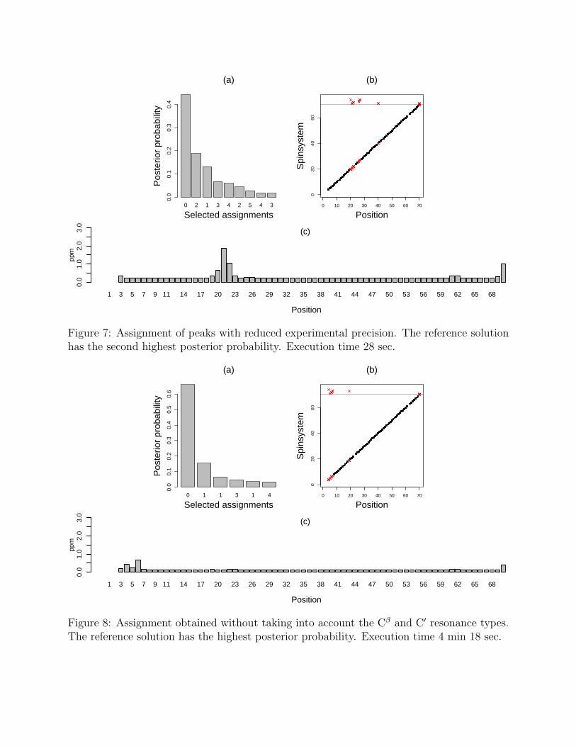
Fig. 8 demonstrates the effect of discarding the chemical shifts of the C′ and Cβ resonancetypes. As shown in the figure, more mappings are plausible than in the original assignment.All of the selected mappings are overall plausible with p-values of their scores exceeding 0.9.Alternative spin systems are mapped to three areas in the primary sequence, namely 4–7, 19and 70. The estimated resonances at positions 4–7 and 70 should be considered as uncertainaccording to the posterior standard deviations.

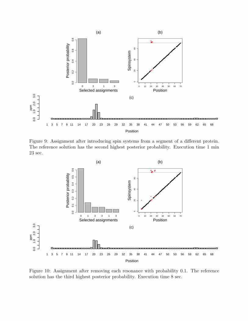
Non-systematic noise. The presence of extra and missing observations cannot bepredicted in advance. Fig. 9 investigates the effect of extra observations by adding spinsystems from a sequential segment of 20 positions of a different protein. A large number ofextras can arise when, for example, a contaminated sample is used, or when the protein hasa second minor conformation. As can be seen from Fig. 9, the assignment procedure selects

0 2 1 3 4 2 5 4 3

0.0

0.1

0.2

0.3

0.4

Selected assignments

Pos

terio

r pr

obab

ility

(a)

0 10 20 30 40 50 60 70

020

4060

Position

Spi

nsys

tem

(b)

1 3 5 7 9 11 14 17 20 23 26 29 32 35 38 41 44 47 50 53 56 59 62 65 68

0.0

1.0

2.0

3.0

(c)

ppm

Position

Figure 7: Assignment of peaks with reduced experimental precision. The reference solutionhas the second highest posterior probability. Execution time 28 sec.

0 1 1 3 1 4

0.0

0.1

0.2

0.3

0.4

0.5

0.6

Selected assignments

Pos

terio

r pr

obab

ility

(a)

0 10 20 30 40 50 60 70

020

4060

Position

Spi

nsys

tem

(b)

1 3 5 7 9 11 14 17 20 23 26 29 32 35 38 41 44 47 50 53 56 59 62 65 68

0.0

1.0

2.0

3.0

(c)

ppm

Position

Figure 8: Assignment obtained without taking into account the Cβ and C′ resonance types.The reference solution has the highest posterior probability. Execution time 4 min 18 sec.

0 3 1 3

0.0

0.2

0.4

0.6

0.8

Selected assignments

Pos

terio

r pr

obab

ility

(a)

0 10 20 30 40 50 60 70

020

4060

Position

Spi

nsys

tem

(b)

1 3 5 7 9 11 14 17 20 23 26 29 32 35 38 41 44 47 50 53 56 59 62 65 68

0.0

1.0

2.0

3.0

(c)

ppm

Position

Figure 9: Assignment after introducing spin systems from a segment of a different protein.The reference solution has the second highest posterior probability. Execution time 1 min23 sec.

0 1 3 3 1 3

0.0

0.1

0.2

0.3

0.4

0.5

0.6

Selected assignments

Pos

terio

r pr

obab

ility

(a)

0 10 20 30 40 50 60 70

020

4060

Position

Spi

nsys

tem

(b)

1 3 5 7 9 11 14 17 20 23 26 29 32 35 38 41 44 47 50 53 56 59 62 65 68

0.0

1.0

2.0

3.0

(c)

ppm

Position

Figure 10: Assignment after removing each resonance with probability 0.1. The referencesolution has the third highest posterior probability. Execution time 8 sec.

0 3 2 3 3 3 3 1 4 3 4 3 3 8 4

0.00

0.05

0.10

0.15

Selected assignments

Pos

terio

r pr

obab

ility

(a)

0 10 20 30 40 50 60 70

020

4060

Position

Spi

nsys

tem

(b)

1 3 5 7 9 11 14 17 20 23 26 29 32 35 38 41 44 47 50 53 56 59 62 65 68

0.0

1.0

2.0

3.0

(c)

ppm

Position

Figure 11: Assignment after adding two first positions in the sequence and introducing twomissing spin systems. Red crosses at positions 5, 6, 11, 12, 33, 44, 51 and 57 indicate thata missing spin system can be successfully mapped to these positions. The reference solutionis not selected. Execution time 3 min 29 sec.

Ubiquitin CspA, positions 3–70 CspA, positions 1–70Condition Matches Sols Time Matches Sols Time Matches Sols Time

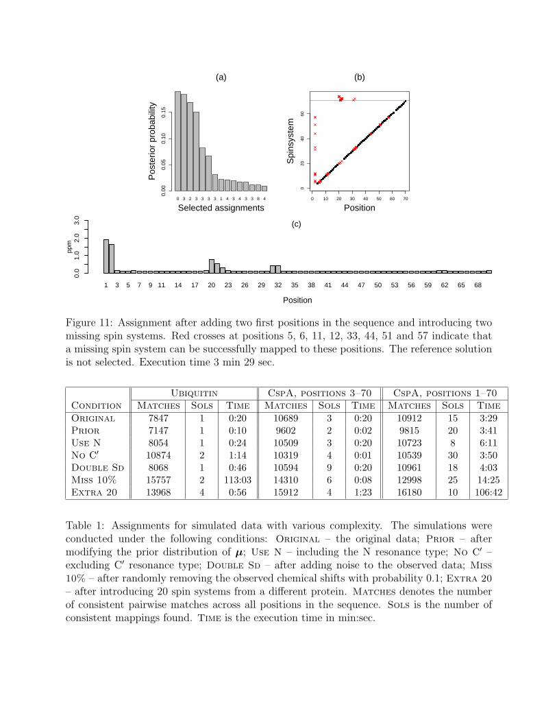
Original 7847 1 0:20 10689 3 0:20 10912 15 3:29Prior 7147 1 0:10 9602 2 0:02 9815 20 3:41Use N 8054 1 0:24 10509 3 0:20 10723 8 6:11No C′ 10874 2 1:14 10319 4 0:01 10539 30 3:50Double Sd 8068 1 0:46 10594 9 0:20 10961 18 4:03Miss 10% 15757 2 113:03 14310 6 0:08 12998 25 14:25Extra 20 13968 4 0:56 15912 4 1:23 16180 10 106:42

Table 1: Assignments for simulated data with various complexity. The simulations wereconducted under the following conditions: Original – the original data; Prior – aftermodifying the prior distribution of µ; Use N – including the N resonance type; No C′ –excluding C′ resonance type; Double Sd – after adding noise to the observed data; Miss

10% – after randomly removing the observed chemical shifts with probability 0.1; Extra 20

– after introducing 20 spin systems from a different protein. Matches denotes the numberof consistent pairwise matches across all positions in the sequence. Sols is the number ofconsistent mappings found. Time is the execution time in min:sec.

one additional mapping containing an extra spin system. All mappings are plausible withp-values of their scores exceeding 0.9.

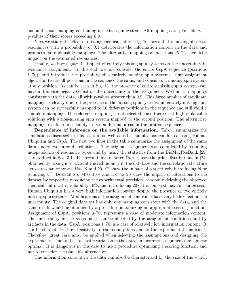
Next we study the effect of missing chemical shifts. Fig. 10 shows that removing observedresonances with a probability of 0.1 deteriorates the information content in the data andproduces more plausible mappings. The alternative mappings at positions 25–26 have littleimpact on the estimated resonances.

Finally, we investigate the impact of entirely missing spin systems on the uncertainty inresonance assignment. To this end, we now consider the entire CspA sequence (positions1–70), and introduce the possibility of 2 entirely missing spin systems. Our assignmentalgorithm treats all positions in the sequence the same, and considers a missing spin systemat any position. As can be seen in Fig. 11, the presence of entirely missing spin systems canhave a dramatic negative effect on the uncertainty in the assignment. We find 15 mappingsconsistent with the data, all with p-values greater than 0.9. This large number of candidatemappings is clearly due to the presence of the missing spin systems: an entirely missing spinsystem can be successfully mapped to 10 different positions in the sequence and still yield acomplete mapping. The reference mapping is not selected since there exist highly plausiblesolutions with a non-missing spin system mapped to the second position. The alternativemappings result in uncertainty in two additional areas in the protein sequence.

Dependence of inference on the available information. Tab. 1 summarizes thesimulations discussed in this section, as well as other simulations conducted using HumanUbiquitin and CspA. The first two lines in the table summarize the assignment of the samedata under two prior distributions. The original assignment was completed by assumingindependence of resonance types and by using the statistics from the BioMagResBank [29]as described in Sec. 3.1. The second line, denoted Prior, uses the prior distributions in [24]obtained by taking into account the redundancy in the database and the correlation structureacross resonance types. Use N and No C′ show the impact of respectively introducing N orremoving C′. Double Sd, Miss 10% and Extra 20 show the impact of alterations to thedataset by respectively reducing the experimental precision, randomly deleting the observedchemical shifts with probability 10%, and introducing 20 extra spin systems. As can be seen,Human Ubiquitin has a very high information content despite the presence of two entirelymissing spin systems. Modifications of the assignment conditions have very little effect on theuncertainty. The original data set has only one mapping consistent with the data, and thesame result would be obtained by a procedure maximizing an appropriate scoring function.Assignment of CspA, positions 3–70, represents a case of moderate information content.The uncertainty in the assignment can be affected by the assignment conditions and byartifacts in the data. CspA, positions 1–70, is a case of relatively low information content. Itcan be characterized by sensitivity to the assumptions and to the experimental conditions.Therefore, great care must be applied when selecting the assumptions and designing theexperiments. Due to the stochastic variation in the data, an incorrect assignment may appearoptimal. It is dangerous in this case to use a procedure optimizing a scoring function, andnot to consider the plausible alternatives.

The information content in the data can also be characterized by the size of the search

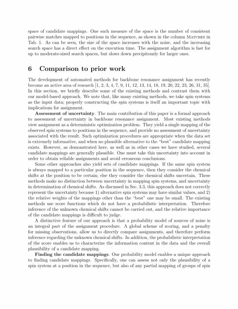
space of candidate mappings. One such measure of the space is the number of consistentpairwise matches mapped to positions in the sequence, as shown in the column Matches inTab. 1. As can be seen, the size of the space increases with the noise, and the increasingsearch space has a direct effect on the execution time. The assignment algorithm is fast forup to moderate-sized search spaces, but slows down precipitously for larger ones.

6 Comparison to prior work

The development of automated methods for backbone resonance assignment has recentlybecome an active area of research [1, 2, 3, 4, 7, 9, 11, 12, 13, 14, 18, 19, 20, 22, 23, 26, 31, 35].In this section, we briefly describe some of the existing methods and contrast them withour model-based approach. We note that, like many existing methods, we take spin systemsas the input data; properly constructing the spin systems is itself an important topic withimplications for assignment.

Assessment of uncertainty. The main contribution of this paper is a formal approachto assessment of uncertainty in backbone resonance assignment. Most existing methodsview assignment as a deterministic optimization problem. They yield a single mapping of theobserved spin systems to positions in the sequence, and provide no assessment of uncertaintyassociated with the result. Such optimization procedures are appropriate when the data setis extremely informative, and when no plausible alternative to the “best” candidate mappingexists. However, as demonstrated here, as well as in other cases we have studied, severalcandidate mappings are generally plausible. One must take this uncertainty into account inorder to obtain reliable assignments and avoid erroneous conclusions.

Some other approaches also yield sets of candidate mappings. If the same spin systemis always mapped to a particular position in the sequence, then they consider the chemicalshifts at the position to be certain; else they consider the chemical shifts uncertain. Thesemethods make no distinction between uncertainty in mapping spin systems, and uncertaintyin determination of chemical shifts. As discussed in Sec. 3.3, this approach does not correctlyrepresent the uncertainty because 1) alternative spin systems may have similar values, and 2)the relative weights of the mappings other than the “best” one may be small. The existingmethods use score functions which do not have a probabilistic interpretation. Thereforeinference of the unknown chemical shifts cannot be carried out, and the relative importanceof the candidate mappings is difficult to judge.

A distinctive feature of our approach is that a probability model of sources of noise isan integral part of the assignment procedure. A global scheme of scoring, and a penaltyfor missing observations, allow us to directly compare assignments, and therefore performinference regarding the unknown chemical shifts. In addition, the probabilistic interpretationof the score enables us to characterize the information content in the data and the overallplausibility of a candidate mapping.

Finding the candidate mappings. Our probability model enables a unique approachto finding candidate mappings. Specifically, one can assess not only the plausibility of aspin system at a position in the sequence, but also of any partial mapping of groups of spin

systems. The plausibility of a partial mapping (and the implications for the plausibility ofa completed assignment) has not been previously used by any other assignment procedure.This results in a significant reduction of the search space, and therefore allows an exhaustivesearch of candidate mappings on problems which were not tractable by previous exhaustivesearch methods. Furthermore, the χ2 interpretation provides an estimate for the upperbound on the total score of the correct assignment, and the penalty allows a meaningfulcomparison of mappings with different numbers of missing observations.

Matching spin systems. All existing methods define the total score as the sum of theindividual contributions, and thus implicitly assume independence of the observed chemicalshifts across positions in the sequence and across resonance types. Furthermore, by employ-ing constant match tolerances or constant parameters for bell-shaped functions that scorematches, all methods implicitly use the assumption of constant variance of chemical shifts.Some algorithms progressively increase match tolerances when no match is found under agiven tolerance, resulting in an arbitrary, unequal treatment of spin systems. We follow theexisting approaches by assuming constant experimental variance of the observed chemicalshifts, but use a flexible scoring function which considers the plausibility of a match jointlyfor all resonance types. Therefore, a relatively loose match of one resonance type can be con-sidered plausible if it is compensated for by very tight matches of the other resonance types.The parameter α controls the overall quality of an acceptable match, and has a probabilisticinterpretation which is not available to the other methods.

Aligning spin systems. The vast majority of the existing methods use a Normalcharacterization of the chemical shifts deposited to a database. In particular, the programMapper [12] uses an almost identical alignment score and its χ2 interpretation. The scorecan be derived from our Bayesian standpoint under the assumption that the resonance typesare a priori independent. However, Mapper assumes pre-compiled chains of spin systems asthe input, and is not concerned with the quality of matching the spin systems. It provides noformal method for statistical inference. Our approach provides a unifying scoring system foraligning and matching, and is capable of incorporating any Normality-based characterizationof the prior distributions.

7 Discussion and future work

To the best of our knowledge, our approach is the first to provide formal statistical inferencefor backbone resonance assignment. We quantify the uncertainty in the assigned chemicalshifts in terms of their posterior standard deviations. We also characterize the informationcontent in the data with a posterior distribution for the set of candidate mappings, and bycomparing the scores of the mappings to the corresponding χ2 distribution. The methodis fully automated and does not require human intervention. It is capable of incorporatingdifferent prior characterizations of chemical shifts and different experimental variances. Itrequires only two tuning parameters, α and β, which control the search space of candidatemappings and are easily interpretable.

We believe that quantification of uncertainty is the key for producing reliable automated

assignments. The use of a single candidate mapping with no quantification of uncertaintycan result in false optimism in the quality of reported chemical shifts. This may lead toerroneous conclusions which in turn may propagate and accumulate through subsequentstages of NMR-based analyses. Reporting posterior standard deviations of the determinedchemical shifts will help prevent such errors. Specific applications of the results of our methodinclude the following. 1) Use only the assigned chemical shifts for which the posteriorstandard deviations are close to the experimental precision. 2) Design additional NMRexperiments based on the posterior standard deviations of chemical shifts, e.g. using isotopiclabeling techniques to probe uncertain residues or residue types, or conducting experimentsthat focus on the resonance types containing most of the uncertainty. 3) Report posteriorstandard deviations of chemical shifts when depositing NMR assignments in public databases,so that entries are annotated according to their uncertainty and the underlying informationcontent. For example, all things being equal, the distributions will help distinguish betweenan assignment based on, say, ten resonance experiments versus one based on just three, orbetween assignments obtained with different spectral resolution. 4) When a single candidatemapping must be used, assess the posterior distribution of the mappings in order to determinethe relative support for the best mapping. At the same time, the score of that mapping willhelp judge its quality of fit with the data.

We plan to improve our method in a number of ways.

1. The space of potential mappings is combinatorially large, and the complexity of theproblem grows exponentially with the protein size. Therefore, even the most effi-cient algorithms for exhaustive search are limited in their use. Inferential algorithmsemploying stochastic search are needed in order to explore large spaces of candidatemappings.

2. The probability model is based on the assumption of constant variance of resonancesassociated with the observed spin systems. However, the resonances are obtained usinga variable number of peaks in the spectra. The quality of the observed peaks varies,and so does the uncertainty associated with their locations. The assumption maybe relaxed in future work by careful modeling of the noise associated with individualpeaks.

3. The current approach considers the candidate mappings with the minimum number ofentirely missing spin systems. However, the penalty (Eq. 4) brings to a common scalemappings with any number of missing spin systems, and mappings with more missingspin systems can in principle have higher posterior probabilities. More research isneeded in order to select an appropriate maximum allowable number of entirely missingspin systems.

4. Additional information, e.g. regarding the secondary structure of the protein, can helpreduce the search space of candidate mappings, as well as the uncertainty associatedwith the assigned chemical shifts. Researchers have attempted to incorporate this

information by means of prediction of secondary structure elements [31]. However, as-sessment of uncertainty in the assigned chemical shifts in this case must incorporate theuncertainty in the prediction. More work is needed to correctly assess the uncertaintyin this case.

The current version of our program, written in Java, can be freely obtained for academicuse by request from the authors.

8 Acknowledgment

We would like to thank Drs. Gaetano Montelione and Hunter Moseley of the Center forAdvanced Biotechnology and Medicine, Rutgers University, for providing access to the datafor Csp A and to the AutoAssign program. This work benefited greatly from discussionswith and help from Dr. Carol Post, Dr. Sampo Mattila and Teri Groesch, Dept. of Biology,Purdue University. This work is funded in part by a US NSF CAREER award to CBK(IIS-0237654).

References

[1] M. Andrec and R. Levy. Protein sequential resonance assignments by combinatorialenumeration using 13Cα, chemical shifts and their (i,i − 1) sequential connectivities.Journal of Biomolecular NMR, 23:263–270, 2002.

[2] H. S. Atreya, S. C. Sahu, K. V. R. Chary, and G. Govil. A tracked approach forautomated NMR assignments in proteins (TATAPRO). Journal of Biomolecular NMR,17:125–136, 2000.

[3] C. Bailey-Kellogg, A. Widge, J. J. Kelley III, M. J. Berardi, J. H. Bushweller, and B. R.Donald. The NOESY Jigsaw: automated protein secondary structure and main-chainassignment from sparse, unassigned NMR data. Journal of Computational Biology,7:537–558, 2000.

[4] C. Bartels, P. Guntert, M. Billeter, and K. Wuthrich. GARANT – a general algorithmfor resonance assignment of multidimensional nuclear magnetic resonance spectra. Jour-nal of Computational Chemistry, 18(1):139–149, 1997.

[5] Y. Benjamini, Y. Hochberg. Controlling the False Discovery Rate: A Practical andPowerful Approach to Multiple Testing. Journal of the Royal Statistical Society, Ser B.57:289-300, 1995.

[6] S. E. Brenner. A tour of structural genomics. Nature Reviews Genetics, 2:801–809,2001.

[7] N. E. G. Buchler, E. P. R. Zuiderweg, H. Wang, and R. A. Goldstein. Protein heteronu-clear NMR assignments using mean-field simulated annealing. Journal of MolecularResonance, 125:34–42, 1997.

[8] J. Cavanagh, W. J. Fairbrother, A. G. Palmer III, and N. J. Skelton. Protein NMRSpectroscopy. Academic Press, 1996.

[9] B. E. Coggins and P. Zhou. PACES: Protein sequential assignment by computer-aidedexhaustive search. Journal of Biomolecular NMR, 26:93–111, 2003.

[10] F. Delaglio, S. Grzesiek, G. W. Vuister, G. Zhu, J. Pfeifer, and A. Bax. NMRPipe: amultidimensional spectral processing system based on UNIX pipes. Journal of Biomolec-ular NMR, 6:277–293, 1995.

[11] W. Gronwald, L. Willard, T. Jellard, R. Boyko, K. Rajarathnam, D. S. Wishart, F. Son-nichsen, and B. Sykes. CAMRA: Chemical shift based computer aided protein NMRassignments. Journal of Biomolecular NMR, 12:395–405, 1998.

[12] P. Guntert, M. Saltzmann, D. Braun, and K. Wuthrich. Sequence-specific NMR as-signment of proteins by global fragment mapping with program Mapper. Journal ofBiomolecular NMR, 17:129–137, 2000.

[13] T. K. Hitchens, J. A. Lukin, Y. Zhan, S. A. McCallum, and G. S. Rule. MONTE: Anautomated Monte Carlo based approach to nuclear magnetic resonance assignment ofproteins. Journal of Biomolecular NMR, 25:1–9, 2003.

[14] T. K. Hitchens, S. A. McCallum, and G. S. Rule. Data requirements for reliable chemicalshift assignments in deuterated proteins. Journal of Biomolecular NMR, 25:11–23, 2003.

[15] Y. Hochberg, A. C. Tamhane. Multiple Comparison Procedures. John Wiley & Sons,1987.

[16] J. A. Hoeting, D. Madigan, A. E. Raftery, and C. T. Volinsky. Bayesian model averaging:A tutorial. Statistical Science, 14(4):382–417, 1999.

[17] R. E. Kass and A. E. Raftery. Bayes factors. Journal of the American StatisticalAssociation, 90(430):773–795, 1995.

[18] M. Leutner, R. M. Gschwind, J. Liermann, C. Schwarz, G. Gemmecker, and H. Kessler.Automated backbone assignment of labeled proteins using the threshold accepting al-gorithm. Journal of Biomolecular NMR, 11:31–43, 1998.

[19] K.-B. Li and B. C. Sanctuary. Automated resonance assignment of proteins using het-eronuclear 3D NMR. 1. Backbone spin systems extraction and creation of polypeptides.Journal of Chemical Informatics and Computational Sciences, 37:359–366, 1997.

[20] G. Lin, D. Xu, Z.-Z. Chen, T. Jiang, and Y. Xu. A branch-and-bound algorithm forassignment of protein backbone NMR peaks. In First IEEE Bioinformatics Conference,pages 165–174, 2002.

[21] J. Liu. Bayesian modeling and computation in bioinformatics research. In T. Jiang,Y. Xu, and M. Zhang, editors, Current topics in computational biology, pages 11–44.MIT Press, 2002.

[22] J. A. Lukin, A. P. Gove, S. N. Talukdar, and C. Ho. Automated probabilistic method forassigning backbone resonances of (13C, 15N)-labeled proteins. Journal of BiomolecularNMR, 9:151–166, 1997.

[23] D. Malmodin, C. Papavoine, and M. Billeter. Fully automated sequence-specific reso-nance assignments of heteronuclear protein spectra. Journal Biomolecular NMR, 27:67–69, 2003.

[24] A. Marin, T. Malliavin, P. Nicholas, M.-A. Delsuc. From NMR chemical shifts toamino acid types: investigation of the predictive power carried by nuclei. Poster atthe Gordon Research Conference on computational aspects of biomolecular NMR, toappear in Journal of Biomolecular NMR, 2004.

[25] G. T. Montelione, D. Zheng, Y. J. Huang, K. Gunsalus, and T. Szyperski. Protein NMRspectroscopy in structural genomics. Nature America Supplement, 2000.

[26] H. N. B. Moseley and G. T. Montelione. Automated analysis of NMR assignments andstructures for proteins. Current Opinions in Structural Biology, 9:635–642, 1999.

[27] S. J. Press. Subjective and Objective Bayesian Statistics : Principles, Models, andApplications. John Wiley & Sons, 2002.

[28] D. B. Rubin. Bayesianly justifiable and relevant frequency calculations for the appliedstatistician. The Annals of Statistics, 12(4):1151–1172, 1984.

[29] B. R. Seavey, E. A. Farr, W. M. Westler, and J. Markley. A relational database forsequence-specific protein NMR data. Journal Biomolecular NMR, 1:217–236, 1991.http://www.bmrb.wisc.edu.

[30] The Ubiquitin NMR Resource Page http://www.biochem.ucl.ac.uk/bsm/nmr/ubq/

[31] X. Wan, D. Xu, C. Slupsky, and G. Lin. Automated protein NMR resonance assign-ments. In Proceedings of the Computational Systems Bioinformatics, 2003.

[32] D.S. Wishart, B.D. Sykes, and F.M. Richards. The chemical shift index: a fast andsimple method for the assignment of protein secondary structure through NMR spec-troscopy. Biochemistry, 31(6):1647–1651, 1992.

[33] K. Wuthrich. NMR of Proteins and Nucleic Acids. John Wiley & Sons, 1986.

[34] H. Zhang, S. Neal, D. S. Wishart. RefDB: a database of uniformely referenced proteinchemical shifts. Journal of Biomolecular NMR, 25:173–195, 2003.

[35] D.E. Zimmerman, C.A. Kulikowski, Y. Huang, W. Feng, M. Tashiro, S. S. Shimotaka-hara, C. Chien, R. Powers, and G. T. Montelione. Automated analysis of protein NMRassignments using methods from artificial intelligence. Journal of Molecular Biology,269:592–610, 1997.