Intra-backbone and Inter-backbone Peering

Among Internet Service Providers∗

Narine Badasyan†and Subhadip Chakrabarti‡

December, 2003

Abstract

We consider a model with two backbones and a finite number of Internet

Service Providers (ISPs) connected to the backbones. ISPs decide on private

peering agreements, comparing the benefits of private peering to costs. Intra-

backbone peering refers to peering between ISPs connected to the same back-

bone, whereas inter-backbone peering refers to peering between ISPs connected

to different backbones. We formulate the model as a two-stage game. In the

first stage, ISPs decide on peering agreements. In the second stage they com-

pete in prices a la Bertrand. We examine the effects of peering on profits of

ISPs. Peering affects profits through two channels - reduction of backbone con-

gestion which we call the symmetric effect and ability to send traffic bypassing

or circumventing congested backbones which we call the asymmetric effect.

The first has a negative or ambiguous effect while the second has a generally

positive effect on firm profits. The two often act against each other making

the net effect ambiguous. We also conduct simulations to determine pairwise

stable peering configurations in a six-provider model and find that there is a

paucity of inter-backbone peering in asymmetric settings.

JEL codes: D21, D43

∗We are indebted to Dr. Robert P. Gilles and Dr. Hans Haller for helpful comments and

suggestions. Our thanks are also due to the participants and discussants in the Southern Economic

Association Meetings, 2003 for their useful comments. The usual disclaimer applies.†Department of Economics, Virginia Tech, Blacksburg, VA 24060, email: nabadsya@vt.edu‡Department of Economics, Virginia Tech, Blacksburg, VA 24060, email: schakrab@vt.edu

1

1 Introduction

The Internet is comprised of many distinct networks, which are operated by different

firms. Each firm has its own network, where the connected users can communicate

with each other. The end-users of the Internet are consumers and websites. End-

users generally want to have access to all other possible end-users, regardless of the

network they are attached to. To provide such universal connectivity to their users,

the firms must interconnect with each other and share their network infrastructure.

Two main forms of interconnection emerged following privatization of the National

Access Points - peering under which firms carry each other’s traffic without any

payments and transit under which the downstream firm pays the upstream firm a

certain settlement payment for carrying its traffic.

Universal connectivity requires some structure on the connectivity agreements.

The Internet has a loosely hierarchical structure (Ross and Kurose, 2000). At the

top of the hierarchy are the backbones, also called Internet Access Providers (here-

after IAPs), that own national and/or international high speed networks. The four

largest IAPs in the U.S. are UUNET/MCI (27.9%), AT&T (10%), SPRINT (6.5%)

and GENUITY/LEVEL3 (6.3%) (Haynal, 2003). The second layer of the hierarchy

includes so called retail Internet Service Providers (hereafter ISPs). At the bottom

of the hierarchy are the end users, i.e. namely consumers who browse the web and

websites.

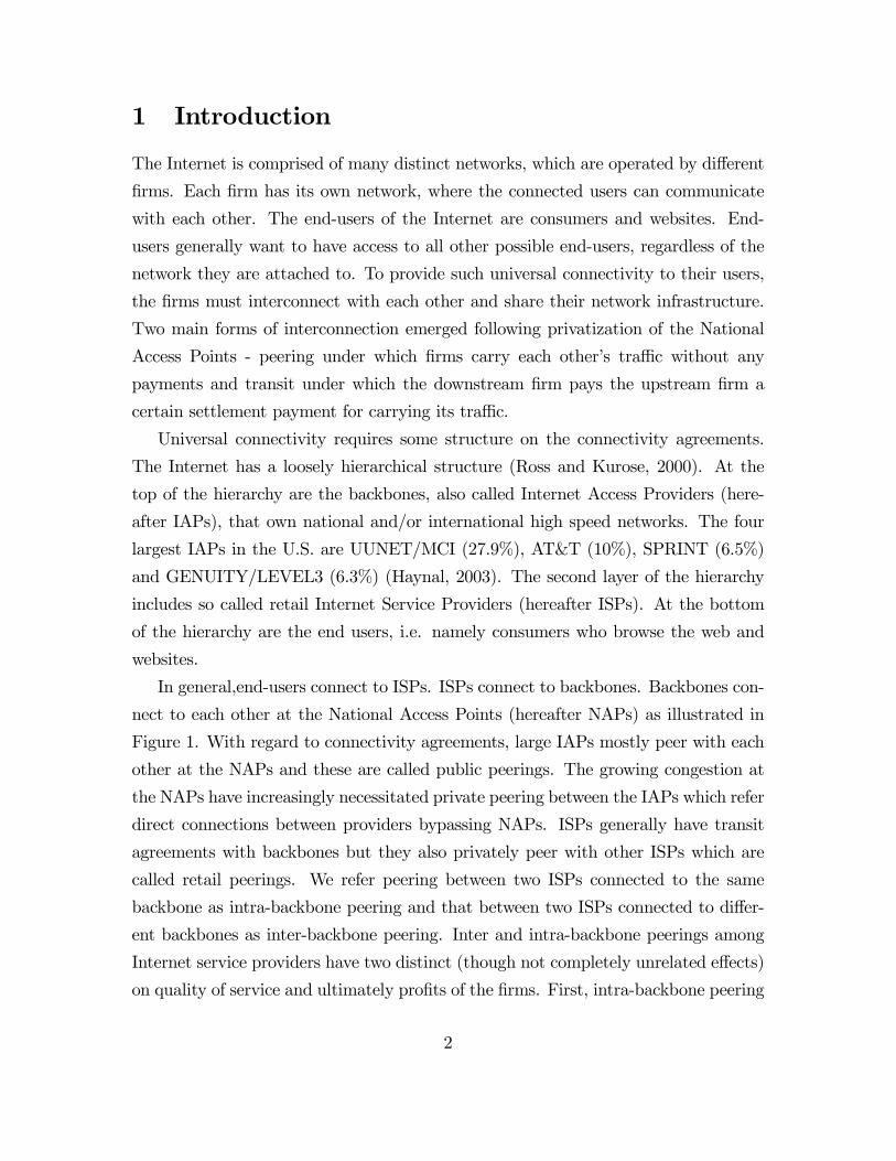
In general,end-users connect to ISPs. ISPs connect to backbones. Backbones con-

nect to each other at the National Access Points (hereafter NAPs) as illustrated in

Figure 1. With regard to connectivity agreements, large IAPs mostly peer with each

other at the NAPs and these are called public peerings. The growing congestion at

the NAPs have increasingly necessitated private peering between the IAPs which refer

direct connections between providers bypassing NAPs. ISPs generally have transit

agreements with backbones but they also privately peer with other ISPs which are

called retail peerings. We refer peering between two ISPs connected to the same

backbone as intra-backbone peering and that between two ISPs connected to differ-

ent backbones as inter-backbone peering. Inter and intra-backbone peerings among

Internet service providers have two distinct (though not completely unrelated effects)

on quality of service and ultimately profits of the firms. First, intra-backbone peering

2

Backbone A Backbone B Backbone C

NAP

ISP

ISP

ISP ISP ISP

ISPISP

ISP

ISP

End users

Private PeeringPublic Peering

Transit Private Peering

Backbone ABackbone A Backbone BBackbone B Backbone CBackbone C

NAP NAP

ISP ISP

ISPISP

ISP ISP ISP ISP ISP ISP

ISPISPISP ISP

ISPISP

ISP ISP

End usersEnd users

Private PeeringPublic Peering

Transit Private Peering

Figure 1:

reduces the traffic within the backbone and raises the quality of all ISPs connected

to that backbone. Inter-backbone peering reduces the traffic between backbones and

raises the quality of all ISPs connected to both backbones. We call this the symmetric

effect or traffic diverting effect. Due to the symmetric effect, peering in general has

strong positive externalities. The chief reason why ISPs may be interested in peering

is not the symmetric effect but the asymmetric effect or the circumventing effect.

Users (both web sites and consumers) who connect through privately peered lines

avoid the congestion/delays associated with going through backbones and National

Access Points. This raises the quality of the ISPs who peer and increases the demand

of those ISPs. We call this the asymmetric or circumventing effect.

The first effect has been captured by DangNyugen and Penard (1999) using a

model of club behavior and vertical differentiation. They consider a model with two

asymmetric backbones and identical retail ISPs connected to those backbones. The

retail ISPs engage in both intra-backbone peering and inter-backbone peering. They

make the assumption that ISPs connected to the same backbone behave like a club

3

and collude with regard to pricing and connectivity behavior. The authors extend

the standard model of vertical product differentiation to show that ISPs connected

to the high quality backbone will always peer with each other. But they may or may

not peer with the ISPs connected to the low quality backbone. Also, in the latter

case, the ISPs of the low quality backbone will peer with each other. The results are

illustrated with some evidence from the French Internet market. The second effect

has been captured among others, by Badasyan and Chakrabarti (2003) who show

that threat of traffic diversion creates strong incentives for peering among backbones

or IAPs.

Before starting the model, we briefly discuss the literature. Generally, one would

expect investment in the Internet infrastructure to be sub-optimal under peering us-

ing the standard argument of the “tragedy of the commons”, given that providers

share a common backbone, especially in presence of large asymmetries. A number of

authors have made this point in a variety of contexts (see Little and Wright (1999),

Cremer et al. (2000)). Such problems can be avoided under transit or settlement

payments. However, transit between large backbones may be impractical given pro-

hibitive costs of monitoring the Internet traffic and may account for the paucity of

transit agreements among large backbones. In the future, when monitoring technol-

ogy improves bringing down monitoring costs, we expect to see peering agreements

being replaced by transit agreements.

There is a related body of literature in Internet economics that deal with pricing

that we mention in passing. Mackie-Mason and Varian (1995) have pointed out that

the current practice of flat-rate pricing (charging a fixed fee to consumers unrelated

to usage) encourages overusage and hence congestion. Their solution to the problem

is setting up a smart market to price consumers according to usage. Of course, this

involves a technological leap but may become feasible in near future.

Currently, Internet services offered by an ISP have little horizontal differentiation

offering the same basic services of web-browsing, emails, real time conversation and

some Internet telephony but there is some vertical differentiation. Some authors

have examined price and product differentiation in services. Odlyzko (1997) suggests

multiservice mechanism, where users can choose between first and second class service

and pay accordingly, even though the quality is not necessarily different. Gibbens

4

et al (2000) discusses the competition between two Internet service providers, when

either or both of them choose to offer multiple service classes. Assuming a uniform

distribution of user preferences towards congestion and a finite number of networks,

they prove that, even when Internet service providers are free to set capacities as

well as prices, multiproduct competition is not sustainable in a profit maximizing

equilibrium.

In this paper, we examine incentives for peering among the retail Internet service

providers taking into account both the symmetric and asymmetric effects, where

ISPs can choose to peer both within and across backbones. A two stage game is

considered. In the first stage, ISPs decide on peering and in the second stage, given the

contractual configuration, they compete a la Bertrand. We find that symmetric and

asymmetric effects of peering often have opposite effects on firms’ profits making the

net effect ambiguous. Hence, the decision to peer or not largely depends on underlying

parameters such as network capacity, number of ISPs connected to each backbone

and number of consumers and websites connected to each ISP. Under simulations

with six ISPs and two backbones, we find that a variety of configurations emerge in

equilibrium depending on the values of the aforesaid parameters.

The rest of the paper is organized as follows. In section 2, we discuss the as-

sumptions underlying the model. In section 3, we analyze the second stage and we

determine equilibrium prices. In section 4, we analyze the first stage and determine

the equilibrium network. Finally, we conclude.

2 The Model

We begin with the assumptions underlying the model. We consider two backbones

A and B and a finite set of N ISPs denoted by η = {1, 2, 3, . . . , N} where N ∈ N.We assume that each ISP is connected to one of the backbones, but not both. Every

ISP has a transit agreement with the backbone it is connected to. According to that

agreement the ISP pays the backbone a certain settlement for interconnection which

is given exogenously. Without loss of generality, we assume that ISPs 1, . . . ,m are

connected to backbone A and ISPs m+ 1, . . . , N are connected to backbone B. Let

ηA = {1, . . . ,m} and ηB = {m+ 1, . . . , N}. Generally we will index backbones by l,

5

Backbone A Backbone B

NAP

ISP1

End users

ISP2 …

ISPm

ISPm+1

…

ISPN

ISPm+2 ISPN-1

Backbone ABackbone A Backbone BBackbone B

NAP NAP

ISP1ISP1

End usersEnd users

ISP2ISP2 …

ISPmISPm

ISPm+1ISPm+1

…

ISPN

ISPm+2 ISPN-1

Figure 2:

l ∈ {A,B} and ISPs by i, j, i, j ∈ η. We illustrate this in Figure 2. We assume that

each ISP pays an access fee (transit) Fl if it is connected to backbone l.We distinguish

between two types of end-users - consumers and websites. There is a continuum of

consumers of mass 1 and a continuum of websites of mass 1 as well. We assume

away any micro-payments from websites to consumers and vice versa. Let αi denote

the proportion of consumers connected to ISP i and di be the proportion of websites

connected to ISP i. Obviously

NXi=1

αi = 1 =NXi=1

di

Also denotemXi=1

αi = α

αi’s are given exogenously. di’s will be determined endogenously by explicit modelling

of website preferences. Thus, α is the proportion of consumers who have chosen the

ISPs connected to backbone A. Similarly, 1− α is the proportion of consumers who

have chosen the ISPs connected to backbone B.

In general it can be asserted that there is little traffic between websites. Traffic

6

between consumers while not negligible are miniscule compared to traffic from web-

sites to consumers. Thus, most of the traffic between the websites and the consumers

is unidirectional, i.e., from websites to consumers. To capture this traffic pattern in

its simplest form, we ignore all traffic between consumers, and from consumers to

websites and focus exclusively on the traffic from websites to consumers. We assume

following Laffont et. al (2001) that consumers are interested in all websites inde-

pendently of their network choices. A consumer is as likely to request a page from

a given website belonging to her network and another website belonging to a rival

network. This is referred in the aforesaid paper as "balanced calling pattern". Hence,

we assume each consumer requests one unit of traffic from each website. This gives

precise measure to the proportion of traffic originating in ISP i and terminating in

ISP j, namely,

tij = di · αj

To be consistent with the standard terminology, we refer to traffic between ISPs

belonging to the same backbone as on-net traffic and traffic going from one backbone

to another as off-net traffic. With regard to traffic movement between backbones,

backbone providers follow what is called “hot potato routing” - pass off net traffic

as soon as possible. Given this pattern of traffic, it is not unrealistic to assume

that all off-net traffic is borne by the receiver backbone. Hence, traffic requested by

consumers in A from websites in B will be borne by backbone A. Similarly, traffic

requested by consumers in B from websites in A will be borne by B.

Let Ui be the utility derived by a website connected to ISP i:

Ui = V − δi − pi

where pi is the price charged by ISP i and δi is the delay associated with ISP i, and

V is the value from the connectivity to the Internet. We assume V to be sufficiently

large so that no consumer drops out of the market.

Delays occur due to excessive traffic in the backbone. Define sl to be the network

capacity of backbone l (l ∈ {A,B}). The network capacity is the maximum amount

of traffic that the backbone can handle without experiencing delay. We assume that

the network capacities are exogenously given. Thus, if tl is the amount of traffic

coming into backbone l, the delay in backbone l is tl − sl.

7

Backbone A Backbone B

NAP

ISP1

End users

ISP2 …ISPm

ISPm+1

…

ISPN

ISPm+2 ISPN-1

Inter-backbone PeeringIntra-backbone Peering

Backbone ABackbone A Backbone BBackbone B

NAP NAP

ISP1ISP1

End usersEnd users

ISP2ISP2 …ISPmISPm

ISPm+1ISPm+1

…

ISPN

ISPm+2 ISPN-1

Inter-backbone PeeringIntra-backbone Peering

Figure 3:

Given the balanced calling pattern and the hot potato routing,

tA =mXi=1

mXj=1

αi · dj +mXi=1

NXj=m+1

αi · dj = α

tB =NX

i=m+1

mXj=1

αi · dj +NX

i=m+1

NXj=m+1

αi · dj = 1− α

ISPs can enter into private peering agreements with each other. If two ISPs build a

private peering link, then that peering is referred to as intra-backbone peering, if the

ISPs are connected to the same backbone, and inter-backbone peering, if the ISPs

are connected to different backbones. For example, in Figure 3, ISP 2 has an intra-

backbone peering agreement with ISP 1 and an inter-backbone peering agreement

with ISP m+2. In order to model private peering, we introduce a standard network

notation borrowed from Goyal and Joshi (2000). For any two distinct ISPs i and j,

define a binary variable gij ∈ {0, 1} where

gij =

(1 if a private peering arrangement exists between i and j

0 if no such arrangement exists

8

Obviously, gij = gji. If gij = 1, we say a link exists or a link is formed between i and

j. The network g = {gij}i,j∈η,i6=j is then a collection of links. Let g − gij denote the

network obtained by severing an existing link between i and j from the network g

while g + gij is the network obtained by adding a new link between i and j in the

network g. The network g for which gij = 1 for all i, j ∈ η, i 6= j is called the complete

network. The network g for which gij = 0 for all i, j ∈ η, i 6= j is called the empty

network.

We assume each private peering link entails a transfer of traffic amounting to σ

between i and j, that is capacity of each private peering link is equal to σ. Usage is

shared equally and costs are borne equally. Assuming quadratic costs, each such link

costs σ2 and the cost borne by each of the two ISPs forming a link is σ2/2.We assume

that the private lines are completely uncongested and hence traffic traversing such

links experience zero delays. Given that private links carry traffic that otherwise

would have been carried by backbones, private peering links also reduce backbone

congestion by reducing backbone traffic.

Now we can compute the average delay experienced by ISP i, namely, δi. Let

nAA denote the number of intra-backbone links for backbone A, nBB be the number

of intra-backbone links for backbone B, and nAB be the number of inter-backbone

links. Obviously,

nll =Xj∈ηl,

Xi∈ηl,i<j

gij

nAB =Xj∈ηB

Xi∈ηA

gij

Further, let niA be the number of links ISP i has with members of ηA and niB be the

number of links ISP i has with members of ηB. Let ni be the total number of private

links of ISP i. Hence,

nil =X

j∈ηl,j 6=igij

ni = niA + niB

Let ωl be the reduction or leakage in the traffic of backbone l as a result of private

9

peerings. Then,

ωA = (nAA) · σ + (nAB) · (σ/2)ωB = (nBB) · σ + (nAB) · (σ/2)

The traffic of backbone l is reduced by the amount of on-net traffic diverted through

intra-backbone private peering links and by the amount of the outgoing off-net traffic

diverted through inter-backbone peering links. Each intra-backbone link reduces on-

net traffic by σ and each inter-backbone link reduces off-net outgoing traffic by σ/2

given that usage of peered links is shared equally.

Hence, if θl is the amount of congestion in backbone l, then

θl = tl − sl − ωl

Traffic going through private peering links experience zero delays because we explicitly

assume that ISPs keep their private links uncongested. All extra traffic is routed

through the backbones. The traffic going through backbone A experience congestion

of θA and the traffic going through backbone B experience a congestion of θB. If

θA > θB, we refer to A as the low quality backbone and B as the high quality

backbone and vice versa.

Consider an ISP connected to backbone A. Given that this ISP has niA intra-

backbone links and each such link can carry σ/2 of traffic, on-net traffic circulating

through privately peered lines is equal to niA · (σ/2) and this traffic experiences zerodelay. Given that total volume of on-net traffic going out from this ISP is α · di, thetraffic that traverses backbone A and experiences a delay of θA is α · di − niA · (σ/2).Next, the off-net traffic going out from this ISP is (1−α) ·di of which again niB ·(σ/2)amount of traffic travels through privately peered lines and experiences zero delay.

Hence, (1 − α) · di − niB · (σ/2) amount of traffic traverses both backbones and islargely borne by the receiver backbone B and hence experiences delay θB. Therefore,

if i ∈ ηA1,

δi = θA · (α · di − niA · (σ/2)) + θB · ((1− α) · di − niB · (σ/2))1Traffic going from websites to consumers connected to the same ISP do not have to traverse any

backbone or private peering link. So strictly speaking, we have to deduct this leakage from traffic

flows through backbones. We assume that this leakage is relatively small and can be ignored.

10

Similarly, if j ∈ ηB,

δj = θB · ((1− α) · dj − njB · (σ/2)) + θA · (α · dj − njA · (σ/2))

Equilibrium demands are determined by equating utilities of all websites given that

in equilibrium all websites must derive an identical utility from each ISP. As far as

the ISPs are concerned, we will analyze a two-stage game. In the first stage, ISPs

form links that determines the network structure g. In the second stage they compete

in prices a la Bertrand. Consistent with the logic of backward induction, we start

with the second stage.

3 Analysis of the Second Stage

Given a certain network g and the fact that firms compete as Bertrand oligopolists, we

can solve for equilibrium prices in the second stage. We show the details in Appendix

1. Here we just present the results in the form of Proposition 1.

Proposition 1 Let ,

γi =σ (niA · θA + niB · θB)

2for all i ∈ ηeθ = α · θA + (1− α) · θB

θA = α− sA − σ³nAA +

nAB2

´θB = (1− α)− sB − σ

³nBB +

nAB2

´The equilibrium price, demand and profit, respectively, of i ∈ ηl in stage 2 is given by

p∗i =

à eθN − 1

!+

1

2N − 1

ÃN · γi −

NXj=1

γj

!(1)

d∗i =

µN − 1N · eθ

¶"Ã eθN − 1

!+

1

2N − 1

ÃN · γi −

NXj=1

γj

!#(2)

π∗i =

µN − 1N · eθ

¶"Ã eθN − 1

!+

1

2N − 1

ÃN · γi −

NXj=1

γj

!#2−µσ2

2

¶ni − Fl (3)

11

Of course, the above proposition represents the unique interior solution. For the

interior solution to exist and be applicable, we need certain parameter constraints.

Specifically, θA > 0 and θB > 0 requires

σ <2(α− sA)

(2 · nAA + nAB)

σ <2(1− α− sB)

(2 · nBB + nAB)sA < α

sB < 1− α

Given that

nAA 6 m(m− 1)2

nBB 6 (N −m)(N −m− 1)2

nAB 6 m(N −m)

we have

2 · nAA + nAB2

6 m(N − 1)2

2 · nBB + nAB2

6 (N −m)(2 ·N − 2 ·m− 1)2

In order to ensure that the above constraints are satisfied for all possible networks,

we assume the following parameter constraints:

0 < sA < α < 1 (4)

0 < sB < 1− α (5)

0 < σ < Min

½2(α− sA)

m(N − 1) ,2(1− α− sB)

(N −m)(2 ·N − 2 ·m− 1)¾

(6)

To allow the possibility of link formation within each backbone, we also assume that

m > 1, N > 3.

We have stated before that θA is the measure of congestion in backbone A and

θB is the measure of congestion in backbone B. The backbone with the lower level of

congestion will be referred to as the high quality backbone and that with the higher

level of congestion will be referred to as the low quality backbone.

12

Hence, eθ = α ·θA+(1−α) ·θB is the level of congestion in each backbone weightedby the traffic flowing through each backbone is an average measure of congestion in

the whole network. eθ captures the symmetric effect of peering because changes inbackbone congestion primarily affect this parameter.

As far as the asymmetric effect is concerned, γi will be referred to as the “link

density factor” of ISP i. It is proportional to the number of links ISP i has in

each backbone weighted by the level of congestion. The weights reflect the fact that

forming links in congested backbones to divert traffic is more valuable than forming

links in uncongested backbones. Next, define

κi = N

Ãγi −

1

N

NXj=1

γj

!

κi which is proportional to the difference between the link density factor of ISP i and

the average link density factor captures the asymmetric effect of peering because it

is proportional to γi which reflects the impact of circumventing congested backbones

on delay.

To see this clearly, we can express the delay or congestion of ISP i, namely δi in

terms of eθ and γi.

δi = di · eθ − γi

Higher the overall backbone congestion, greater is the delay, but delay can be

reduced by increasing the link density factor because traffic can now circulate through

uncongested lines. Increasing demand also increases delay because larger amount of

the traffic passes through congested backbones.

We can express prices, demands and profits in terms of eθ and κi.

p∗i =

à eθN − 1

!+

µκi

2N − 1¶

d∗i =

µN − 1N · eθ

¶"Ã eθN − 1

!+

µκi

2N − 1¶#

π∗i =

µN − 1N · eθ

¶"Ã eθN − 1

!+

µκi

2N − 1¶#2−µσ2

2

¶ni − Fl

13

By gross profits we mean profits gross of link formation costs or profits not taking

into account link formation costs. Hence, gross profit is simply the product of price

and demand minus the transit fee paid to the backbones. We can examine the impact

that symmetric and asymmetric effects of peering have on gross profits.

Next let us examine how peering affects gross profits. First note that

∂pi

∂eθ =1

N − 1 > 0

∂di

∂eθ =−(N − 1) · κi

(2 ·N − 1) ·N ·³eθ´2 < 0 if κi > 0 and > 0 if κi < 0.

Hence, increasing the level of overall congestion increases prices.2 For ISPs with

above average link density, increasing the level of congestion reduces demand while

reducing the link density increases demand. For ISPs with below average link density,

the opposite is the case. Increasing the level of overall congestion increases demand

and vice versa.

Now an intra-backbone link reduces eθ by ασ through its effect on the backbone

the ISPs belong to. An inter-backbone link reduces eθ by σ/2 through its impact on

both backbones. While those boost consumer utilities, they have either a negative

or an ambiguous effect on firm profits. For ISPs with below average link density

(κi < 0) the impact is definitely negative because given the signs of the derivatives

above, both prices and demands fall and hence gross profits fall. For ISPs with above

average link density (κi < 0), the impact is ambiguous. While prices fall, demands

rise and hence the net effect depends on the relative magnitudes of the two effects.

It is somewhat counter-intuitive that peering should have a negative or ambiguous

effect on gross profit. This is because the effect of reducing overall congestion on price

is always negative. This is because,

δi − δj = (di − dj) · eθ − (γi − γj)

Hence, any increase in eθ accentuates the difference in quality or congestion or thelevel of vertical differentiation between firms i and j. The increase in vertical differ-

entiation softens price competition and enables both firms to charge higher prices.

In fact, both prices rise by an exactly equal amount in equilibrium and hence final

2This is a standard result for congested goods (see De Palma and Leruth (1989)).

14

differences in prices as well as differences in congestion remain unchanged. Hence the

initial increase in the difference in congestion is compensated by appropriate changes

in demands.

Next, consider the asymmetric effects of peering. We have

∂pi∂κi

=1

2 ·N − 1 > 0

∂di∂κi

=(N − 1)

(2 ·N − 1) ·N · eθ > 0

Consider the impact of intra and inter-backbone links on κi. There is a direct

effect owing to the fact the traffic can now travel through uncongested lines and

there is an indirect effect owing to the impact of link formation on congestion in

the backbones θA and θB. We ignore the indirect effect because it involves terms σ2

which is negligible if σ is small. Thus an intra-backbone link for i ∈ ηl boosts κi byN · σ · θl

2and hence has a positive impact on gross profits. An inter-backbone link

increases κi byσ[(N − 1)θ−l − θl]

2where −l refers to the backbone other than l. If i

belongs to the high quality backbone, namely, θ−l > θl, inter-backbone links increase

gross profits. If i belongs to the low quality backbone, θ−l < θl, inter-backbone links

increase gross profits provided the quality difference between the two backbones is

not very high, i.e. (N − 1)θ−l > θl. However, if the quality difference between the

two backbones is very high, (N − 1)θ−l < θl, then inter-backbone peering has indeed

a negative effect on gross profits.

Hence we get Proposition 2.

Proposition 2 (a) For ISPs with link density that is below the average link density,

the symmetric effects of intra-backbone or inter-backbone peering on gross profits are

always negative. For those with link density above the average, the effect is ambigu-

ous.

(b) For all ISPs, the asymmetric effect of intra-backbone peering on gross profits is

always positive. For ISPs connected to high quality backbones, the effect of inter-

backbone peering is also positive. However, for ISPs connected to low quality back-

bones, the effect is positive if the difference in quality between the two backbones is

sufficiently small and negative otherwise.

15

We can summarize these facts in form of the following tables. Let HH denote the

fact that the ISP in question belongs to the high quality backbone and has higher

than average link density. Let HL denote the fact that the ISP in question belongs

to the high quality backbone and has lower than average link density. Let LH denote

the fact that the ISP in question belongs to the low quality backbone and has higher

than average link density. Let LL denote the fact that the ISP in question belongs

to the low quality backbone and has lower than average link density.

_____________________________________________

Table 1: Effect of peering on gross profit when (N − 1)θ−l > θl

Intra-backbone Peering

Symmetric

Effect

Asymmetric

Effect

Inter-backbone Peering

Symmetric

Effect

Asymmetric

Effect

HH Ambiguous Positive Ambiguous Positive

HL Negative Positive Negative Positive

LH Ambiguous Positive Ambiguous Positive

LL Negative Positive Negative Positive_____________________________________________

Table 2: Effect of peering on gross profit when (N − 1)θ−l < θl

Intra-backbone Peering

Symmetric

Effect

Asymmetric

Effect

Inter-backbone Peering

Symmetric

Effect

Asymmetric

Effect

HH Ambiguous Positive Ambiguous Positive

HL Negative Positive Negative Positive

LH Ambiguous Positive Ambiguous Negative

LL Negative Positive Negative Negative_____________________________________________

Hence, one finds that quite often the symmetric effect and asymmetric effects

actually work against each other. This is because while peering improves quality

and hence prices, demands and profits, its effect on backbone congestion has the

unintended effect of reducing vertical differentiation, stiffening price competition and

reducing prices and profits. The net effect us almost always ambiguous and stating

anything further would require comparison of relative magnitudes which in turn would

depend on relative values of parameters α, sl and m. Hence one would expect to find

16

a multitude of equilibrium networks depending on the values of these parameters, a

fact that we illustrate in the next section with simulations.

However, we can state one thing with certainty. If the quality difference between

the two backbones is substantial, namely (N − 1)θA < θB or vice versa, then ISPs

connected to the quality backbone have no interest in interpeering if it also has lower

than average link density. This is because gross profits reduce with inter-backbone

peering given that both the symmetric and asymmetric effects are negative, and the

added cost of link formation further reduces net profits. This actually forms the basis

of Proposition 3.

4 Analysis of the First Stage

We will analyze the first stage using the notion of pairwise stability which was in-

troduced by Jackson and Wolinsky (1996). A network is pairwise stable if given the

network, there is no incentive to either form links or destroy links. Since links are

formed unilaterally but can be broken bilaterally, we can formally define it as follows:

Definition: Let πi(g) denoted the reduced profits of stage 1 for a network g. The

network g is pairwise stable if for all i, j ∈ η :

(a) If gij = 1, then πi(g) > πi(g − gij) and πj(g) > πj(g − gij)

(b) If gij = 0 and πi(g + gij) > πi(g), then πj(g + gij) < πj(g)

The intuition here is quite simple. Links are formed bilaterally but can be broken

unilaterally. Hence, in a pairwise stable network, neither player should gain by break-

ing a link while at least one player must lose or remain indifferent through forming a

new link.

Before we embark on simulations, let us formalize our analysis in the previous

section in the form of Proposition 3.

Proposition 3 Let (N − 1)θ−l < θl where l represents the low quality backbone,

namely the quality differential between the two backbones is sufficiently large. Then,

in any pairwise stable network, there will be no inter-backbone peering between two

ISPs with different link densities if the ISP belonging to the low quality backbone has

lower than average link density.

17

In all other cases, given that net effects of peering are ambiguous, we cannot

state anything for certain. However, we can do some simulations. We will only

study six-provider networks. The choice of six is not entirely arbitrary. Since the

number of ISPs attached to each backbone has to be greater than or equal to two

for any meaningful analysis, six is the smallest number that allows us to consider

both symmetry as well asymmetry in the number of firms attached to individual

backbones. We will consider only the following eight possible cases or eight possible

networks.3

1. All ISPs peer with each other. The resulting network called a complete network

is denoted by gAB1.

2. There is no peering whatsoever. The resulting network called an empty network

is denoted by g000.

3. All ISPs belonging to both backbones engage in intra-backbone peering but

there is no inter-backbone peering. We refer to the resulting network by gAB0.

4. All ISPs belonging to backbone A engage in intra-backbone peering. How-

ever there is neither any inter-backbone peering nor any intra-backbone peering in

backbone B. We refer to this network as gA00.

5. All ISPs belonging to backbone B engage in intra-backbone peering. How-

ever there is neither any inter-backbone peering nor any intra-backbone peering in

backbone A. We refer to this network as g0B0.

6. All ISPs belonging to backbone A engage in intra-backbone peering. There

is no intra-backbone peering in backbone B but there is inter-backbone peering. We

refer to this network as gA01.

7. All ISPs belonging to backbone B engage in intra-backbone peering. There

is no intra-backbone peering in backbone A but there is inter-backbone peering. We

refer to this network as g0B1.

8. No intra-backbone peering whatsoever but there is inter-backbone peering.

We refer to this network as g001.

Case 1: We start with perfect symmetry, namely, α = 0.5, m = 3, sA = sB = s

(say). Then the area where all parameter constraints (4)-(6) are satisfied is repre-

3Checking more complicated networks for pairwise stability requires some programming which is

reserved as a future endeavour.

18

sented by figure 4 where we plot σ and s along the two axes. This figure and all

subsequent figures are in Appendix 2. We will refer to the parameter range for which

constraints (4)-(6) are satisfied as the feasible parameter range or the feasible range.4

We find that with complete symmetry, two networks are pairwise stable in the

feasible parameter range, namely, the complete network and the empty network.

Figure 5 represents the area where the complete network is pairwise stable. Figure

6 represents the area where the empty network is pairwise stable. The two areas

represent mutually exclusive parameter ranges, hence, for a given set of parameter

values, there is an unique pairwise stable network which is either the complete or

the empty network. This is clear from Figure 7 where we represent the two areas in

the same figure. Under complete symmetry, all firms face exactly the same benefits

and costs. Hence, it is expected that we get symmetric outcomes, namely either all

firms will peer or nobody will peer. Depending on the magnitudes of σ and s either

outcome is feasible.

Case 2: Next we will introduce asymmetries. We find that introduction of

asymmetries result in other pairwise stable networks. We begin with an asymmetry

in the network capacity. Specifically, assume that sA > sB = s. We plot σ, sA and

sB = s along the three axes. We find that there are two additional pairwise stable

network configurations within the feasible parameter range besides the complete and

the empty network, namely, the network gAB0 and the network g0B0. We summarize

this in figures 8 to 12. The figures are three dimensional to account for the fact

that sA and sB are represented in two different axes. Figure 8 represents the feasible

parameter range. Figure 9 represents the area where the complete network is pairwise

stable. Figure 10 represents the area where the empty network is pairwise stable.

Figure 11 represents the area where the network gAB0 is pairwise stable. Figure 12

represents the area where the network g0B0 is pairwise stable.

Case 3: Next, starting from perfect symmetry, let us introduce an asymmetry in

the number of firms connected to each backbone. Here our options are quite limited.

We can consider only the case where m = 4 and n = 6. We plot σ and s(= sA = sB)

on the two axes. We find that again there are two possible pairwise stable networks

4The figures have by developed using Mathematica. Computations are available at

www.filebox.vt.edu/users/schakrab/computations.htm.

19

besides the complete and the empty network in the feasible parameter range, namely,

the network gAB0 and the network g0B0. We represent this situation in figure 13 to

18. Figure 13 represents the feasible parameter range. Figure 14 represents the

area where the complete network is pairwise stable. Figure 15 represents the area

where the empty network is pairwise stable. Figure 16 represents the area where the

network gAB0 is pairwise stable. Figure 17 represents the area where the network g0B0is pairwise stable. The areas are mutually exclusive hence for a certain parameter

value we get an unique stable network. This can be seen from figure 18 where we

bring all the different areas in one figure.

Case 4: Finally, let us explore asymmetries in the consumer base. Assume,

for instance, starting from a perfectly symmetric setup with n = 6, that α > 0.5.

We represent this situation in figure 19 to 23. The figures are three dimensional

and we plot α, σ and s(= sA = sB) along the three axes. This time we find that

besides the complete and the empty network, two more networks namely gAB0 and

gA00 are pairwise stable within the feasible parameter range. Figure 19 represents the

feasible parameter range. Figure 20 represents the area where the complete network

is pairwise stable. Figure 21 represents the area where the empty network is pairwise

stable. Figure 22 represents the area where the network gAB0 is pairwise stable.

Figure 23 represents the area where the network gA00 is pairwise stable.

We summarize these results of our simulations in the form of Proposition 4.

Proposition 4 Let n = 6 and parameter values satisfy constraints (4)-(6). Then, (1)

for complete symmetry, namely, α = 0.5,m = 3 and sA = sB, there are two pairwise

stable networks, namely the complete network and the empty network; (2) for an

asymmetry in the network capacity, namely, α = 0.5,m = 3 and sA > sB, there are

four pairwise stable networks, namely the complete network, the empty network, gAB0and g0B0. (3) for an asymmetry in the number of firms connected to each backbone,

namely, α = 0.5,m = 4 and sA = sB, there are four pairwise stable networks, namely

the complete network, the empty network, gAB0 and g0B0 (4) for an asymmetry in the

consumer base, namely, α > 0.5,m = 3 and sA = sB, there are four pairwise stable

networks, namely the complete network, the empty network, gAB0 and gA00.

20

We summarize this in the following table.

Table 3

Nature of asymmetry Pairwise Stable Networks

None gAB1, g000

Asymmetry in network capacity sA > sB gAB1, g000, gAB0, g0B0

Asymmetry in the the number of firms m > n/2 gAB1, g000, gAB0, g0B0

Asymmetry in the website base α > 1/2 gAB1, g000, gAB0, gA00We find there are two major trends in our simulations:

(a) First, when ISPs connected to backbones whose congestion without taking to

account leakage due to peering (θl+ωl) is higher tend to intrapeer, the ISPs belonging

to the other backbone do not intrapeer.

(b) There is no interpeering in presence of asymmetries in networks other than

the complete network.

Now, (b) could be partly a due to the proposition 2 especially given the fact that

N is small. But there is likely other effects that we are unable to capture in a formal

manner.

We will briefly compare our results with that of DangNyugen and Penard (1999).

In their model, ISPs connected to each backbone collude with each other and behave

like a club while ours is a purely non-cooperative game. Further, in their model,

the only asymmetry is with regard to an exogenously given quality, while in ours

there are many sources of asymmetry and quality is determined endogenously by a

complex interaction of several factors. Their model only takes the symmetric effect

into account while ours take both effects into account. If we extend their results in

context of pairwise stability, one would be likely to observe the network configuration

gA00, gAB0 and g0B0 depending on whether A or B is the high quality backbone. We

also find that in our simulations, these three networks recur with some regularity.

However, depending on parameter values, two other networks namely, the complete

and empty network are also pairwise stable.

5 Conclusions

We find that there are two main avenues by which peering affects gross profits. The

impact on the quality of service offered by the firm given that traffic can circumvent

21

congested backbones which we term the asymmetric effect and the impact on back-

bone congestion which we term the symmetric effect. The asymmetric effect generally

increases gross profits and the symmetric effect has a negative or ambiguous impact

on gross profits. The two effects often work against each other making the net effect

ambiguous as well.

One may object to this paper on the grounds that it does not have a punch

line. Yet, it is precisely that absence of a punchline that we strive to show. Retail

peering has quite complicated effects on firm profits and it is by no means certain that

improving the quality of service by forming peering agreements would automatically

increase gross profits even if we disregard the costs of peering. Peering among retail

ISPs have both a positive and negative effect with regard to gross profits. On the

positive side, peering improves quality, increases demand and enables firms to charge

higher prices. On the negative side, it reduces differentiation and promotes stiffer

price competition. Also, it may lead to overuse of one’s network without adequate

reciprocity. The relative magnitude of these factors help or hinder peering. In complex

settings, such magnitudes also quite complex to analyze and give rise to a multitude of

configurations depending on the various exogenously determined factors. This paper

helps to illustrate this with the help of simulations.

22

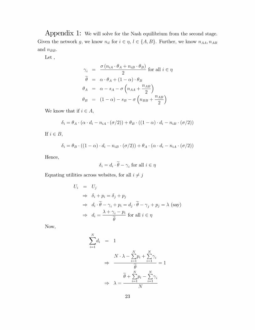
Appendix 1: We will solve for the Nash equilibrium from the second stage.

Given the network g, we know nil for i ∈ η, l ∈ {A,B}. Further, we know nAA, nAB

and nBB.

Let ,

γi =σ (niA · θA + niB · θB)

2for all i ∈ ηeθ = α · θA + (1− α) · θB

θA = α− sA − σ³nAA +

nAB2

´θB = (1− α)− sB − σ

³nBB +

nAB2

´We know that if i ∈ A,

δi = θA · (α · di − niA · (σ/2)) + θB · ((1− α) · di − niB · (σ/2))

If i ∈ B,

δi = θB · ((1− α) · di − niB · (σ/2)) + θA · (α · di − niA · (σ/2))

Hence,

δi = di · eθ − γi for all i ∈ η

Equating utilities across websites, for all i 6= j

Ui = Uj

⇒ δi + pi = δj + pj

⇒ di · eθ − γi + pi = dj · eθ − γj + pj = λ (say)

⇒ di =λ+ γi − pieθ for all i ∈ η

Now,

NXi=1

di = 1

⇒N · λ−

NPi=1

pi +NPi=1

γieθ = 1

⇒ λ =

eθ + NPi=1

pi −NPi=1

γi

N

23

Hence,

di =

µ1eθ¶·

eθ + NP

j=1

pi −NPj=1

γi

N

+ γi − pi

=

1

N+

µ1

N · eθ¶Ã NX

j=1

(pj − γj)−N · (pi − γi)

!

=1

N+

µ1

N · eθ¶ÃX

j 6=i(pj − γj)− (N − 1) · (pi − γi)

!(7)

The above equation gives us equilibrium demands for all ISPs. Next we will solve

for equilibrium prices. Profits for ISP i are given by

πi = pi · di − Ci

where costs of ISP i connected to backbone l are given by

Ci =

µσ2

2

¶· ni + Fl

Since Ci does not depend on prices, it can be treated as a constant.

Hence,

pi · di =piN+

µpi

N · eθ¶ÃX

j 6=i(pj − γj)− (N − 1) · (pi − γi)

!

=piN+

µpi

N · eθ¶ÃX

j 6=i(pj − γj)

!−µN − 1N · eθ

¶· (p2i − γi · pi)

∂πi∂pi

=1

N+

µ1

N · eθ¶ÃX

j 6=i(pj − γj)

!−µN − 1N · eθ

¶· (2 · pi − γi) = 0

⇒ pi =

µ1

2 ·N − 1¶·"eθ + NX

j=1

pj −NXj=1

γj +N · γi#

LetNXj=1

pj = ep and NXj=1

γj = eγ24

.

Then

pi =

µ1

2 ·N − 1¶·heθ + ep− eγ +N · γi

iSumming up for all i,

ep =

µN

2 ·N − 1¶··eθ + ep− eγ] +µ N

2 ·N − 1¶· eγ¸

=

µN

2 ·N − 1¶· (eθ + ep)

⇒ ep = eθ ·NN − 1

Hence,

pi =

µ1

2 ·N − 1¶·"eθ + eθ ·N

N − 1 −NXj=1

γj +N · γi#

=eθ

N − 1 +µ

1

2N − 1¶Ã

N · γi −NXj=1

γj

!(8)

The above equation gives us equilibrium prices. From the above two equations,

after some manipulation, we get equilibrium demand of ISP i :

di =

µN − 1N ∗ eθ

¶" eθN − 1 +

µ1

2N − 1¶Ã

N · γi −NXj=1

γj

!#(9)

Hence the profits are given by:

πi =

µN − 1N ∗ eθ

¶" eθN − 1 +

µ1

2N − 1¶Ã

N · γi −NXj=1

γj

!#2−µσ2

2

¶· ni − Fl (10)

where ISP i is connected to backbone l.

25

Appendix 2:.

0.005 0.01 0.015 0.02 0.025 0.03 s

0.1

0.2

0.3

0.4

0.5sB

0.005 0.01 0.015 0.02 0.025 0.03 s

0.1

0.2

0.3

0.4

0.5sB

Figure 40.005 0.01 0.015 0.02 0.025 0.03 s

0.1

0.2

0.3

0.4

0.5sB

0.005 0.01 0.015 0.02 0.025 0.03 s

0.1

0.2

0.3

0.4

0.5sB

Figure 40.002 0.004 0.006 0.008 0.01 0.012 0.014 s

0.05

0.1

0.15

0.2

sB

0.002 0.004 0.006 0.008 0.01 0.012 0.014 s

0.05

0.1

0.15

0.2

sB

Figure 50.002 0.004 0.006 0.008 0.01 0.012 0.014 s

0.05

0.1

0.15

0.2

sB

0.002 0.004 0.006 0.008 0.01 0.012 0.014 s

0.05

0.1

0.15

0.2

sB

Figure 50.005 0.01 0.015 0.02 0.025 0.03

s

0.1

0.2

0.3

0.4

0.5sB

0.005 0.01 0.015 0.02 0.025 0.03s

0.1

0.2

0.3

0.4

0.5sB

Figure 60.005 0.01 0.015 0.02 0.025 0.03

s

0.1

0.2

0.3

0.4

0.5sB

0.005 0.01 0.015 0.02 0.025 0.03s

0.1

0.2

0.3

0.4

0.5sB

Figure 6

0.005 0.01 0.015 0.02 0.025 0.03 s

0.1

0.2

0.3

0.4

0.5sB

0.005 0.01 0.015 0.02 0.025 0.03 s

0.1

0.2

0.3

0.4

0.5sB

Figure 7

0.005 0.01 0.015 0.02 0.025 0.03 s

0.1

0.2

0.3

0.4

0.5sB

0.005 0.01 0.015 0.02 0.025 0.03 s

0.1

0.2

0.3

0.4

0.5sB

Figure 7

00.010.020.03s

0

0.2

0.4S

0

0.2

0.4

Sa

00.010.020.03s

0

0.2

0.4S

Figure 8

00.010.020.03s

0

0.2

0.4S

0

0.2

0.4

Sa

00.010.020.03s

0

0.2

0.4S

Figure 800.0050.01

s

00.05

0.10.15

0.2

S

0

0.05

0.1

0.15

0.2

Sa

00.0050.01s

00.05

0.10.15

0.2

S

Figure 900.0050.01

s

00.05

0.10.15

0.2

S

0

0.05

0.1

0.15

0.2

Sa

00.0050.01s

00.05

0.10.15

0.2

S

Figure 9

00.010.020.03s

00.1

0.20.3

S

0

0.1

0.2

0.3

0.4

Sa

00.1

0.20.3

S

Figure 10

00.010.020.03s

00.1

0.20.3

S

0

0.1

0.2

0.3

0.4

Sa

00.1

0.20.3

S

Figure 10

00.0050.010.015s

00.05

0.10.15

0.2

S

0

0.05

0.1

0.15

0.2

Sa

00.0050.010.015s

00.05

0.10.15

0.2

S

Figure 11

00.0050.010.015s

00.05

0.10.15

0.2

S

0

0.05

0.1

0.15

0.2

Sa

00.0050.010.015s

00.05

0.10.15

0.2

S

Figure 11

00.0050.010.0150.02s

0 0.05 0.1 0.15 0.2S0

0.2

0.4

0.6

0.8

Sa

Figure 12

00.0050.010.0150.02s

0 0.05 0.1 0.15 0.2S0

0.2

0.4

0.6

0.8

Sa

Figure 120.005 0.01 0.015 0.02 0.025 s

0.1

0.2

0.3

0.4

0.5sB

0.005 0.01 0.015 0.02 0.025 s

0.1

0.2

0.3

0.4

0.5sB

Figure 13

0.005 0.01 0.015 0.02 0.025 s

0.1

0.2

0.3

0.4

0.5sB

0.005 0.01 0.015 0.02 0.025 s

0.1

0.2

0.3

0.4

0.5sB

Figure 13

0.002 0.004 0.006 0.008 0.01 0.012s

0.05

0.1

0.15

0.2

sB

0.002 0.004 0.006 0.008 0.01 0.012s

0.05

0.1

0.15

0.2

sB

Figure 14

0.002 0.004 0.006 0.008 0.01 0.012s

0.05

0.1

0.15

0.2

sB

0.002 0.004 0.006 0.008 0.01 0.012s

0.05

0.1

0.15

0.2

sB

Figure 14

0.005 0.01 0.015 0.02 s

0.1

0.2

0.3

0.4

0.5sB

0.005 0.01 0.015 0.02 s

0.1

0.2

0.3

0.4

0.5sB

Figure 15

0.005 0.01 0.015 0.02 s

0.1

0.2

0.3

0.4

0.5sB

0.005 0.01 0.015 0.02 s

0.1

0.2

0.3

0.4

0.5sB

Figure 15

0.0025 0.005 0.0075 0.01 0.0125 0.015 s

0.05

0.1

0.15

0.2

sB

0.0025 0.005 0.0075 0.01 0.0125 0.015 s

0.05

0.1

0.15

0.2

sB

Figure 16

0.0025 0.005 0.0075 0.01 0.0125 0.015 s

0.05

0.1

0.15

0.2

sB

0.0025 0.005 0.0075 0.01 0.0125 0.015 s

0.05

0.1

0.15

0.2

sB

Figure 16

0.005 0.01 0.015 0.02 0.025s

0.05

0.1

0.15

0.2

sB

0.005 0.01 0.015 0.02 0.025s

0.05

0.1

0.15

0.2

sB

Figure 17

0.005 0.01 0.015 0.02 0.025s

0.05

0.1

0.15

0.2

sB

0.005 0.01 0.015 0.02 0.025s

0.05

0.1

0.15

0.2

sB

Figure 17

0.005 0.01 0.015 0.02 0.025 s

0.1

0.2

0.3

0.4

0.5sB

0.005 0.01 0.015 0.02 0.025 s

0.1

0.2

0.3

0.4

0.5sB

Figure 18

0.005 0.01 0.015 0.02 0.025 s

0.1

0.2

0.3

0.4

0.5sB

0.005 0.01 0.015 0.02 0.025 s

0.1

0.2

0.3

0.4

0.5sB

Figure 18

00.010.020.03s

0

0.2

0.4

S

0.5

0.6

0.7

0.8

a

00.010.020.03s

0

0.2

0.4

S

Figure 19

00.010.020.03s

0

0.2

0.4

S

0.5

0.6

0.7

0.8

a

00.010.020.03s

0

0.2

0.4

S

Figure 19

00.0050.01s

0

0.05

0.1

0.15

0.2

S

0.50.5250.55

0.575

0.6

a

00.0050.01s

0

0.05

0.1

0.15

0.2

S

Figure 2000.0050.01

s

0

0.05

0.1

0.15

0.2

S

0.50.5250.55

0.575

0.6

a

00.0050.01s

0

0.05

0.1

0.15

0.2

S

Figure 20

00.010.020.03s

0

0.2

0.4

S

0.50.55

0.6

0.65a

00.010.020.03s

0

0.2

0.4

S

Figure 21

00.010.020.03s

0

0.2

0.4

S

0.50.55

0.6

0.65a

00.010.020.03s

0

0.2

0.4

S

Figure 21

00.0050.010.015s

00.05

0.10.15

0.2

S0.5

0.6

0.7

0.8

a

Figure 22

00.0050.010.015s

00.05

0.10.15

0.2

S0.5

0.6

0.7

0.8

a

Figure 22

00.010.020.03s

0

0.2

0.4

S

0.50.55

0.6

0.65a

00.010.020.03s

0

0.2

0.4

S

Figure 23

00.010.020.03s

0

0.2

0.4

S

0.50.55

0.6

0.65a

00.010.020.03s

0

0.2

0.4

S

Figure 23

.

26

References

[1] Badasyan, N., and Chakrabarti, S. (2003) “Private Peering Among Internet

Backbone Providers”, mimeo

[2] Cremer, J.; Rey, P. and Tirole, J. (2000)“Connectivity in the Commercial Inter-

net”, The Journal of Industrial Economics, vol. XLVIII, no. 4, pp.433-472.

[3] Cukier, K. (1998a) The Global Internet: a primer. Telegeography 1999. Wash-

ington D.C. pp.112-145.

[4] Cukier, K. (1998b) “Peering and Fearing: ISP Interconnection and Regulatory

Issues”, http://ksgwww.harvard.edu/iip/iicompol/Papers/Cukier.html.

[5] DangNguyen, G. and Penard, T. (1999), “Interconnection between ISP, Capacity

Constraints and Vertical Differentiation” ; mimeo

[6] De Palma, A. and Leruth, L. (1989), “Congestion and Game in Capacity: A

Duopoly Analysis in the Presence of Network Externalities”, Annales d’Economie

et de Statistique, no.15/16, pp.389-407.

[7] Economides, N. (1996) “The Economics of Networks,” International Journal of

Industrial Organization, vol. 14, no. 6, pp. 673-699 (October 1996).

[8] Gibbens, R., Mason, R., Steinberg, R. (2000) “Internet Service Classes under

Competition”, IEEE Journal on Selected Areas in Communication, v18, no.12,

pp.2490-2498.

[9] Goyal S., and Joshi, S. (2000) “Networks of Collaboration in Oligopoly” , mimeo

[10] Hall, Eric A. (2000) Internet Core Protocols: A Definite Guide, O’REILLY

[11] Haynal, Russ “Russ Haynal’s ISP Page”, http://navigators.com/sessphys.html

[12] Jackson, Matthew O.; Wolinsky, Asher; “A Strategic Model of Social and Eco-

nomic Networks”; Journal of Economic Theory; Vol. 71, No. 1; October, 1996;

44-74; #2685.

27

[13] Kende, M. (2000) “The Digital Handshake: Connecting Internet Backbones”,

Federal Communications Commission, OPP working Paper No. 32

[14] Kurose, J. and Ross, K., Computer Networking:A Top-Down Approach Featuring

the Internet , Addison-Wesley, preliminary edition, 2000.

[15] Laffont, J.J.; Marcus, S.; Rey, P. and Tirole, J. (2001)“Internet Interconnection

and the Off-Net-Cost Pricing Principle”, mimeo

[16] Little, I. and Wright, J. (2000)“Peering and Settlement in the Internet: An

Economic Analysis”, Journal of Regulatory Economics, v. 18, no. 2: pp.151-173.

[17] Mackie-Mason, J. K. and Varian, Hal R. (1995) “Pricing the Internet”, Public

Access to the Internet, Brian Kahin and James Keller, eds. Cambridge, MA: MIT

Press, pp. 269-314.

[18] Mackie-Mason, J. K. and Varian, Hal R. (1995) “Pricing Congestable Network

Resources”, IEEE journal on Selected Areas in Communications, v13, no.7,

pp.1141-1149.

[19] Mason, R. (2001) “Compatibility Between Differentiated Firms With Network

Effects”, University of Southampton, Discussion Paper in Economics and Econo-

metrics, No. 9909.

[20] Mason, R. (2000) “Simple Competitive Internet Pricing”, European Economic

Review, v44, no.4-6, pp.1045-1056.

[21] Odlyzko, A. (1999) “Paris Metro Pricing for the Internet”, Proc. ACM Confer-

ence on Electronic Commerce, ACM, pp.140-147

[22] Pappalardo, Denise (05/30/2001) “The ISP top dogs”,

http://www.nwfusion.com/newsletters/isp/2001/00846039.html, Network

World Internet Services Newsletter.

[23] Shneider Gary P. and Perry, James T. (2001) Electronic Commerce, Course

Technology.

28

[24] TeleGeography. (2000) Hubs and Spokes: A TeleGeography Internet Reader.

Washington, DC: TeleGeography, Inc.

[25] Tirole, J. (1988) The Theory of Industrial Organization, Cambridge, MA and

London, England: MIT Press

29