MLSSA SPO Manual 4WI Rev 8 (2)

MLSSA SPO

Speaker Parameter Option

Reference Manual

Version 4WI

Rev 8

DRA Laboratories

Copyright 1991-2005 by Douglas D. Rife

All rights reserved.

www . mlssa . com

CONTENTS

0. SOFTWARE LICENSE AGREEMENT .................................................................. 1

1. Introduction ......................................................................................................... 5

2. Installation ........................................................................................................... 11

3. Reference............................................................................................................ 13 3.1 Overview of Speaker Parameter Option ...................................................... 13 3.2 DCR modes Measuring Driver DC Resistance ....................................... 17 3.3 Drive Level and Proximity Effects ................................................................ 22 3.4 Measured Parameters.................................................................................. 25 3.5 Closed-box Method ...................................................................................... 28 3.6 Added-mass Method .................................................................................... 32 3.7 Fixed-Mmd Method ...................................................................................... 35 3.8 Indirect Measurement of Sd ......................................................................... 37 3.9 Quality Control Features .............................................................................. 38 3.10 Exporting Parameters................................................................................. 42 3.11 Synthesizing Driver Impedance ................................................................. 43

4. Procedures.......................................................................................................... 45 4.1 Direct Measurement Procedure ................................................................... 45 4.2 Power Amplifier Measurement Procedure ................................................... 53 4.3 Acoustic Frequency Response + Parameters Procedure............................ 61 4.4 Production QC Tips ...................................................................................... 71

5. Bibliography ........................................................................................................ 73

Appendix A Menu Trees .......................................................................................... 75

Appendix B Equations.............................................................................................. 77 Symbol definitions and units................................................................................. 77 Electrical Q and total Q equations........................................................................ 78 Equations for closed-box method......................................................................... 78

iii

Equations for added-mass method.......................................................................79 Equations for Fixed-Mmd method.........................................................................79 Other parameters..................................................................................................79

iv

0. SOFTWARE LICENSE AGREEMENT

NOTICE READ BEFORE INSTALLING THE SOFTWARE

MLSSA SPEAKER PARAMETER OPTION ("SPO") PROGRAM LICENSE AGREEMENT

OF DRA LABORATORIES ("VENDOR")

CAREFULLY READ THE TERMS AND CONDITIONS OF THIS AGREEMENT BEFORE INSTALLING THE SPO SOFTWARE. INSTALLING THE SOFTWARE INDICATES YOUR ACCEPTANCE OF THESE TERMS AND CONDITIONS. IF YOU DO NOT AGREE WITH THE TERMS AND CONDITIONS OF THIS AGREEMENT, PROMPTLY RETURN THE COMPLETE SPO PROGRAM INCLUDING ALL DOCUMENTATION TO THE PLACE OF PURCHASE FOR REFUND IN THE AMOUNT YOU PAID.

1. Definitions

The SPO Program is licensed (not sold) to you, and DRA Laboratories owns all copyright, trade secret, patent and other proprietary rights in the SPO Program. The term "SPO Program" includes all copies of the MLSSA Speaker Parameter Option program overlay, supporting utility programs, supporting calibration data files and all associated documentation.

2. License

a. Authorized Use. Vendor grants you a nonexclusive license to run the SPO Program on a single computer owned directly by you or your company.

b. Restrictions. You may not: (1) distribute, rent, lease or sublicense all or any portion of the SPO Program to third parties; (2) modify or prepare derivative works of the SPO Program; (3) transmit the SPO Program over a network, by telephone, or electronically using any means to third parties; or (4) reverse engineer, decompile or disassemble the SPO Program. You agree to keep confidential and use your best efforts to prevent and protect the contents of the SPO Program from unauthorized disclosure or use.

c. Transfer. You may transfer the SPO Program, but only if the recipient agrees to accept the terms and conditions of this Agreement. If you transfer the SPO Program, you must transfer all associated computer programs and documentation and erase any copies residing on your computer equipment. Your license is automatically terminated if you transfer the SPO Program.

3. Limited SPO Program Warranty

For 30 days from the date of shipment, we warrant that the media (for example, diskette) on which the SPO Program is contained will be free from defects in materials and workmanship. This warranty does not cover damage caused by improper use or neglect. We do not warrant the contents of the SPO Program or that it will be error free. The SPO Program is furnished "AS IS" and without warranty as to the performance or results you may obtain by using the SPO Program. The entire risk as to the results and performance of the SPO Program is assumed by you. To obtain warranty service during the 30-day warranty period, you may return the SPO Program (postage paid) with a description of the problem to Vendor. The defective media in which the SPO Program is contained will be replaced at no additional charge to you.

page 2

License

4. Remedy

If you do not receive media which is free from defects in materials and workmanship during the 30-day warranty period, you will receive a refund for the amount you paid for the SPO Program provided all associated media and documentation supplied to you is returned undamaged to the point of purchase.

5. Disclaimer of Warranty And Limitation of Remedies

YOU UNDERSTAND AND AGREE AS FOLLOWS:

a. THE WARRANTIES IN THIS AGREEMENT REPLACE ALL OTHER WARRANTIES, EXPRESS OR IMPLIED, INCLUDING ANY WARRANTIES OF MERCHANTABILITY OR FITNESS FOR A PARTICULAR PURPOSE. WE DISCLAIM AND EXCLUDE ALL OTHER WARRANTIES. IN NO EVENT WILL OUR LIABILITY OF ANY KIND INCLUDE ANY SPECIAL, INCIDENTAL OR CONSEQUENTIAL DAMAGES, INCLUDING LOST PROFITS, EVEN IF WE HAVE KNOWLEDGE OF THE POTENTIAL LOSS OR DAMAGE.

b. We will not be liable for any loss or damage caused by delay in furnishing a SPO Program or any other performance under this Agreement.

c. Our entire liability and your exclusive remedies for our liability of any kind (including liability for negligence except liability for personal injury caused solely by our negligence) for the SPO Program covered by this Agreement and all other performance or nonperformance by us under or related to this Agreement are limited to the remedies specified by this Agreement.

d. Some states do not allow the exclusion of implied warranties, so the above exclusion may not apply to you. This warranty gives you specific legal rights, and you may also have other rights which vary from state to state.

MLSSA SPO Reference Manual Version 4WI Rev 8 DRA Laboratories, copyright 1991-2005 by Douglas D. Rife page 3

6. Termination

This Agreement is effective until terminated. You may terminate it at any time by destroying the SPO Program, including all computer programs and documentation, and erasing any copies residing on computer equipment. This Agreement also will terminate if you do not comply with any terms or conditions of this Agreement. Upon such termination you agree to destroy the SPO Program and erase all copies residing on computer equipment.

7. U.S. Government Restricted Rights

The SPO Program is provided to the Government only with restricted rights and limited rights. Use, duplication, or disclosure by the Government is subject to restrictions set forth in FAR Sections 52-227-14 and 52-227-19 or DFARS Section 52.227-7013(C)(1)(ii), as applicable. Manufacturer is DRA Laboratories, 4587 Cherrybark CT, Sarasota, FL 34241.

8. General

You are responsible for installation, management and operation of the SPO Program.

page 4

Introduction

1. Introduction

The mathematical representation or modeling of dynamic loudspeakers by a lumped-parameter LRC resonant circuit is due mainly to the work of A. N. Thiele and R. H. Small [1, 2] and is generally known as the Thiele-Small model. The values of these hypothetical inductors, resistors and capacitors and their associated electrical, acoustical and mechanical constants are known as the Thiele-Small parameters. This simple electrical model of driver behavior has significantly advanced the art of loudspeaker design over the last three decades by its ability to make accurate predictions of loudspeaker system performance based on a few simple equations.

Like all models, however, the Thiele-Small model is only an approximation to actual non-ideal driver behavior. Any real driver is a complicated and weakly nonlinear device. Nonlinearity stems from several sources including: variation of the suspension's compliance with displacement [4, Figure 2]; mechanical hysteresis of the suspension also called creep [4, Figure 2] and; nonuniform magnetic flux density surrounding the voice coil resulting in variations in the transduction factor Bl with cone displacement [5, Figure 5]. Richard Small has commented on some of the limitations of his model [2] but his caveats are often forgotten by modern loudspeaker designers. One should always keep in mind that no real driver behaves exactly as predicted by the Thiele-Small model. Therefore, any technique for measuring the driver parameters should take into account the non-ideal driver behavior.

In addition to nonlinearity, another complicating characteristic of real drivers is their motor impedance. Motor impedance can be defined as the impedance vs. frequency curve exhibited by a driver when its voice coil is blocked (mechanically prevented from moving). In the past, motor impedance was often referred to as an "inductive rise in impedance at high frequencies" but this description is inadequate since motor impedance cannot be accurately modeled as a simple inductor. Better models of motor impedance have been derived by Vanderkooy [6] and Wright [7]. In any event, driver


motor impedance should either be eliminated or accounted for when measuring the Thiele-Small parameters.

Conventional methods for measuring the driver parameters based on driver impedance measurements do not account for the non-ideal driver behavior. This is the case with the original measurement method devised by Thiele [1] and described in detail by Small in [2]. Thiele's method derives the parameters from just three special impedance points and considers only impedance magnitude while ignoring impedance phase. These special impedance points comprise the peak value plus the two points on either side of the peak that are exactly 3 dB down after subtracting the DC resistance component. The main problem with Thiele's method is its lack of noise immunity. That is, if just one of the three selected impedance points happens to be deviant due either to measurement noise or to driver anomalies, the resulting parameters will be unrepresentative of the overall driver behavior.

Furthermore, to precisely locate these three special impedance points requires very fine frequency resolution leading to long measurement times regardless of the measurement method employed. This is due to the time-frequency uncertainty principle, which states that the minimum measurement time equals the reciprocal of the desired frequency resolution. For example, a 0.1 Hz frequency resolution requires at least a 10 second measurement time using any measurement technique. While sweeping analyzers can skip over the undesired impedance points their sweep rate must approach zero near the desired points and then sufficient settling time must elapse before an accurate reading can be made. MLSSA, in contrast, can simultaneously measure a large number of linearly spaced impedance points in the same time interval required by a sweeping analyzer to measure just three points. With Thiele's method, however, these "extra" impedance points are discarded meaning that the enormous time-bandwidth product advantage of MLSSA is effectively wasted.

Because real drivers do not conform exactly to the parameter model, optimal measurement methods have been devised. An optimal method determines the set of parameters which, when taken together, best fits the actual non-ideal driver behavior over some time or frequency range of interest. The "best fit" criterion means finding that unique set of driver parameters that minimizes the mean squared error between

page 6

Introduction

the impedance curve predicted by the model and the actual measured driver impedance. Linear regression analysis and all other common forms of curve fitting use this least squared error (LSE) criterion. Thiele's original method of parameter measurement, while useful, is not optimal since three impedance points are far to few to apply any optimal curve fitting method. The assumption implicit in the original method is that these three impedance points lie exactly on some theoretically perfect impedance curve when, in fact, this is rarely the case.

Furthermore, as stated above, the noise immunity of Thiele's method is poor this also being due to relying on only three impedance points. For instance, if just one impedance point happens to be deviant due to 60 Hz hum pickup by the voice coil, the computed parameters will be totally invalidated. Optimal methods, in contrast, consider large numbers of data points so that the effect of one or a few deviant points is insignificant to the analysis.

An example of an optimal parameter measurement technique is due to Leach et al [8]. In this method, a current step function is applied to the driver and the resulting time-domain voltage response is recorded. This is, in effect, a time-domain "impedance" measurement. The LSE criterion is then applied to fit a portion of the driver's step-response to the Thiele-Small equations. To reduce the deleterious effects of the driver's electrical motor impedance, the initial portion of the step response is excluded from the analysis. This works because the typical effects of motor impedance in the time domain are localized to the initial portion of the step response. The main disadvantage of this method, like all time-domain methods, is that it cannot easily confine the analysis frequency range to a particular region. Neither can it readily correct for other devices in the measuring chain such as antialiasing filters.

These disadvantages of optimal time domain methods can be overcome by applying the LSE criterion to driver impedance in the frequency domain as exemplified by the MLSSA Speaker Parameter Option (SPO). Driver impedance is, of course, a complex function of frequency. That is, each impedance point has both a real and imaginary part or, in polar coordinates, a magnitude and a phase part. Thus, driver impedance can be envisioned as a curve in 3D space where the X-axis represents the real part of the impedance, the Y-axis the imaginary part and the Z-axis represents frequency.


SPO determines the driver parameters by performing an optimal 3D curve fit to the driver impedance over a user-specified frequency range. This complex curve-fitting method is also optimal in a LSE sense but, unlike optimal time-domain methods, the analysis frequency range can be set arbitrarily and measurement errors due to the antialiasing filter or other devices in the measuring chain are easily corrected for. In contrast to Leach's time-domain method, any competing frequency domain method must somehow account for the driver's motor impedance over the analysis frequency range of interest.

SPO accounts for the motor impedance through a simple but effective lump-parameter electrical model. The model consists of a lossless inductance in series with a lossy (damped) inductance. While not as accurate as the models of Vanderkooy [6] or Wright [7] over the entire audio band, it is sufficiently accurate to obtain a good fit to the driver’s measured motor impedance from DC up to about 100 times the driver's resonant frequency Fs.

In summary, SPO finds the unique set of driver parameters which best fits, in an LSE sense, the actual driver behavior over the frequency range of interest. In addition, both the magnitude and phase of the measured complex impedance are considered simultaneously. The fit is the optimal because no other set of parameters can be found which will yield a better fit (that is, yield a lower mean squared error) between the Thiele-Small model and the measured complex impedance over the frequency range of interest. This 3D curve-fitting technique should not be confused with conventional curve fitting methods which consider only impedance magnitude or, which employ general purpose fitting functions (e.g. cubic splines) that do not necessarily conform to the Thiele-Small parameter model. SPO, in contrast, fits only those 3D impedance curves that conform to the Thiele-Small model. The resulting parameters obtained by the 3D curve fit are therefore necessarily the best possible representation of actual driver behavior within the limitations of the Thiele-Small model.

Another significant advantage of SPO is its ability to detect driver rub problems. Anything that disturbs the free movement of the voice coil in the air gap such as direct contact with the magnet structure or the presence of foreign matter such as metal chips or debris in the air gap will be directly reflected as nonlinearity into the motional

page 8

Introduction

impedance. Due to the phase randomization property of MLS methods, this nonlinearity will result in increased roughness in the measured impedance curve. To exploit this effect, SPO provides an additional parameter that is a measure of impedance roughness. This parameter, called the Rub-index, can therefore be used as a very sensitive rub indicator. Note however that certain buzz problems will not show up as roughness in the measured impedance curve if the cause (e.g. a flapping piece of surround material) is not strongly coupled to the voice coil. Therefore, certain types of rare buzz noises can only be detected acoustically or by a human listener.


Installation

2. Installation

The MLSSA Speaker Parameter Option (SPO) is supplied as an overlay file named COMPARMS.OVL plus some additional help and setup files. MLSSA will automatically load this file from the default MLSSA directory when the invoking the Library Parameters command from the frequency domain.

MLSSA SPO is licensed to you for use with one particular pair of AFM-50 filter modules mounted on one particular MLSSA card. The hyphenated pair of 4-digit numbers (DDDD-DDDD) handwritten on your SPO installation diskette should agree with the last four digits of the corresponding pair of 8-digit AFM-50 serial numbers. If not, SPO will not run properly. The same hyphenated pair of 4-digit numbers should also be handwritten on your MLSSA installation diskette. If your MLSSA card is already installed, press Alt-3 from the main MLSSA menu and check that the displayed pair of numbers agrees with the pair handwritten on your SPO installation diskette. Assuming you have the correct SPO installation diskette for that particular MLSSA card, insert the diskette into drive A and from Windows 95/98 click Start then Run and enter:

a:install.exe

then click OK.

From the DOS prompt type

a:install <Enter>

and follow the directions given by the install program.

Note that SPO must be installed into the same directory as MLSSA. Additionally, the version of SPO must be compatible with the version of MLSSA. If they are not compatible the error message "Installed option's version number is not up to date!" will appear when you attempt to access SPO through the Library Parameters command from the frequency domain. If you encounter this error, you will need to upgrade your MLSSA software before proceeding.


Reference

3. Reference

3.1 Overview of Speaker Parameter Option

MLSSA SPO determines the driver parameters by analyzing the driver's complex impedance over the frequency range of interest. Unlike the conventional 3-point method, however, all of these complex impedance points are used in the analysis. The conventional method uses only three impedance points [1, 2]. If one or more of these points happens to be deviant due to measurement noise or to driver anomalies, the results can be unrepresentative of the actual driver behavior.

Driver impedance is complex and can be envisioned as a curve in 3D space where the X axis represents the real part of the impedance, the Y axis the imaginary part and the Z axis represents frequency. In the complex curve-fitting method, the Thiele-Small model is expressed a rational polynomial over the complex plane (i.e. as a function of the Laplace variable s). Then the pole and zero locations of this polynomial are adjusted to minimize the mean squared error between it (on the imaginary axis) and the measured complex impedance. The Thiele-Small parameters are then derived from these optimum pole and zero locations. This method therefore finds the unique set of driver parameters that best fits the magnitude and phase of measured impedance over any user-selected frequency range. Furthermore, the curve fit is optimum in an LSE (least squared error) sense: No other set of parameters can be found which will yield a better fit between the Thiele-Small model and the actual measured complex impedance over the frequency range of interest.

Note that SPO, when performing the 3D curve fitting, weights the complex impedance data points according to 1/f, where f is frequency. This is done to compensate for the increasing density of impedance data points, on a per octave basis, with increasing frequency. The 1/f weighting function used by SPO is equivalent to equal weighting if the impedance data points were uniformly distributed on a log frequency scale.

The electrical equivalent circuit of the model used in the analysis is shown in the figure below.


Driver Electrical Equivalent Circuit

The voice coil's electrical behavior, called motor impedance, is modeled as a series resistance (Re), a series lossless inductance (L1) and a series lossy inductance (L2 || R2). This model of motor impedance suffices over the useful frequency range of driver (up to about 100 times Fs) but becomes increasingly inaccurate at higher frequencies. Nevertheless, this simple model is sufficiently accurate over the useful frequency range of the driver to be useful in simulations.

The electrical capacitance Cmes models the driver's total moving mass including the air load. It is related to the driver's actual total moving mass, Mms, by:

Cmes = Mms/(Bl)2,

where Bl is the driver's transduction constant given in units of Tesla-meters. Note that Bl normally varies as a function of cone displacement so that the value given here must be interpreted as an effective or average value taken over the cone displacement range produced by the MLS test signal. Note also that the value of Bl as measured by SPO is determined under dynamic conditions and therefore may not agree exactly with static Bl measurements. This effect is due to the reluctance force [4], which only appears when the voice coil is in motion.

page 14

Reference

The electrical inductance, Lces, models the driver's mechanical compliance. It is related to the driver's actual mechanical compliance, Cms, by:

Lces = Cms·(Bl)2.

Finally, because mechanical compliance devices (e.g. springs) always exhibit losses the parallel resistance Res is added to model these losses in electrical terms. Res is related to the driver's actual mechanical losses, Rms, by:

Res = (Bl)2/Rms.

Taken as a whole, this electrical equivalent circuit can be described mathematically as a rational polynomial over the complex plane comprising three poles and four zeros.

The SPO analysis window is defined by the marker and cursor positions in the frequency domain. It should extend from the lowest reliable frequency to well above the impedance valley. The impedance valley is the first minimum in impedance magnitude above the driver's resonant frequency Fs. The lowest reliable frequency is determined by the low frequency cut-off of the power amplifier, which should extend down to well below Fs for accurate results. If a DC-coupled amplifier is used or, if the impedance is measured by direct connection to MLSSA, the low frequency point should extend down to the first impedance point above DC. The DC point itself must not be included in the analysis window because MLS methods inherently reject DC. When the signal path to the driver is DC coupled, SPO can be configured to measure the true DC resistance of the driver via a separate measurement using a DC stimulus.

The analysis frequency range should extend up to at least four times the impedance valley frequency to insure that the parameters related to motor impedance (L1, L2 and R2) are determined correctly. Otherwise, the curve-fitting algorithm may become indeterminate and fail or, if successful, the accuracy of the T/S parameters may be compromised. These potential problems can occur because the driver's motor impedance component often has little effect upon total driver impedance at frequencies around and below the impedance valley. Therefore, there will be insufficient information to determine L1, L2 and R2 with precision when there is insufficient high frequency impedance data is included in the analysis window.


While the impedance valley of large woofers typically lies well below 1 kHz, this is not normally the case for smaller woofers and multimedia drivers. To correctly analyze headphone drivers, multimedia drivers and tweeters, MLSSA must be set up to measure driver impedance over wider bandwidth to ensure that SPO has a sufficiently wide analysis frequency range to achieve a reliable fit. For small woofers and mid-range drivers, with resonant frequencies in the range of 30 Hz to 100 Hz a measurement bandwidth of 4 kHz is recommended. For headphone and multimedia drivers, with resonant frequencies in the range of 100 Hz to 300 Hz, a 10 kHz measurement bandwidth is recommended. For small multimedia drivers and tweeters with resonant frequencies in the range of 300 Hz to 1 kHz, a 20 kHz measurement bandwidth is recommended. To accommodate these different driver types SPO includes four MLSSA setup files: SPO1K.SET for large woofers; SPO4K.SET for small woofers and mid-range drivers; SPO10K.SET for multimedia drivers; and SPO20K.SET for small multimedia drivers and tweeters.

After performing the 3D curve fit, SPO internally reconstructs the impedance curve and determines the frequency of the impedance valley. The reconstructed impedance curve is used to locate the valley to insure that measurement noise will not influence the result. Then the valley frequency is compared with ¼ of the upper frequency limit of the analysis window, as set by the cursor or marker. If the impedance valley frequency is greater than ¼ of the upper frequency limit of the analysis frequency range, the parameter calculations are aborted and the message “Insufficient HF impedance data included in analysis window: ” is displayed followed by the analysis window frequency range you had chosen. If you receive this error message, widen the analysis window to include more high frequency impedance data or, if need be, chose a new setup file having the next larger bandwidth. For example, if you were using SPO1K.SET change to SPO4K.SET or if you were using SPO4K.SET change to SPO10K.SET.

page 16

Reference

3.2 DCR modes Measuring Driver DC Resistance

SPO provides four methods or modes for determining the driver's DC resistance (DCR). The four DCR modes are named Fixed, Measure, Estimate #1 and Estimate #2 as selected through the DCR-mode command from the Library Parameters menu.

The Fixed DCR mode allows you to manually enter the driver’s DC resistance, Re, as measured by an ohmmeter or DVM. The Fixed DCR mode forces the fitted impedance curve to pass through whatever value you enter for Re at zero frequency. However, because the test leads connecting MLSSA to the driver add their own residual DC resistance, significant errors in the quality of the curve fit can occur in the Fixed DCR mode unless care is taken to correct for this residual test lead resistance. Therefore, the DC resistance of your test leads should measured and entered into SPO through the DCR-mode Calibrate Manual command described later in this section. Because of the need to manually measure the driver’s DC resistance with a DVM and manually enter that value into SPO, the Fixed DCR mode is cumbersome and not recommended unless you are making impedance measurements through an AC-coupled power amplifier and require the highest possible accuracy.

The Measure DCR mode directs SPO to perform a separate data acquisition sequence using a DC stimulus to achieve accurate DCR measurements automatically every time the Go command is executed. The applied DC stimulus amplitude is the same as the current MLSSA stimulus output level as set by the Acquisition Stimulus Amplitude command. Driver DCR is actually measured twice, first with a positive polarity DC stimulus and then with a negative polarity stimulus. This two-step measurement sequence eliminates the effects of any DC offsets in the signal path due, for example, to a power amplifier or, to thermocouple voltages generated when different metals are in contact. Such small DC voltages can arise when the test lead clips, for example, are not made of the same metal as the driver terminals. As a result, the Measure mode achieves accuracy comparable to all but the highest quality DVMs. Note here that the Measure DCR mode must only be used if you are certain that the signal path to the driver is truly DC-coupled. Some power amplifiers incorporating DC servo loops may appear to be DC-coupled but are actually AC coupled, having a very low cut-off


frequency of just a few Hz. Attempting to use such amplifiers with the Measure DCR mode will result in severe measurement errors of the driver’s DC resistance.

For highest accuracy of parameter measurements, the Measure DCR mode is recommended when the signal path to the driver is DC-coupled, including direct measurements made without a power amplifier as well as measurements made through a power amplifier that is known to be DC coupled.

The Estimate #1 and Estimate #2 DCR mode are entered through the DCR-mode Estimate command, which asks if the path to the driver is DC coupled. If you answer ‘Y’, the Estimate #1 DCR mode is automatically entered. If you answer ‘N’, the Estimate #2 DCR mode is entered automatically.

Estimate #1 DCR mode uses real part of the lowest frequency AC impedance point as the driver DCR. This DCR mode is not as accurate as the Measure DCR mode on drivers having a low resonant frequency (Fs < 30 Hz). In addition, the Estimate # 1 DCR mode is more sensitive to measurement noise than the Measure DCR mode resulting in more variation in Re from one measurement to the next. Nevertheless, the Estimate #1 DCR mode can be used in many cases with acceptable results. One slight advantage of the Estimate #1 DCR mode over the Measure DCR mode is speed. The Estimate #1 DCR mode requires absolutely no extra time to measure driver DCR. Consider using this DCR mode when speed is paramount and the signal path to the driver is DC coupled or, when the power amplifier is AC coupled but still has significant response down to 1 Hz. In most cases, the Measure mode is preferable due to its higher accuracy, but can only be used when the signal path is truly DC coupled.

The Estimate #2 mode uses curve fitting alone to extrapolate the impedance curve down to DC from the available AC impedance data falling within the analysis window. The Estimate #2 DCR mode is the least accurate DCR mode but it is the only choice when the signal path to the driver is AC coupled, its frequency response does not extend down to subsonic frequencies and the Fixed DCR mode method is too slow or too cumbersome to consider using.

page 18

Reference

In all DCR modes, there is a potential for measurement errors due to the DC resistance of the test leads. This error can be significant with long leads or low gauge cable. Any error in a driver's measured DC resistance directly affects parameters Re, Qes and Qts. In the Fixed DCR mode, uncorrected test lead DC resistance is even more insidious because it can cause significant curve fitting errors. To avoid these errors, SPO provides for measuring and removing the effects of residual test lead resistance through the DCR-mode Calibrate commands. The Auto option should be selected only when the signal path is truly DC coupled. This command first asks you to open the test leads to perform a DC gain reference measurement and then asks you to short them together to measure and store the residual test lead DC resistance. (Note if the MLSSA RCAI is connected, you will only be prompted to short your test leads briefly to measure their residual series DC resistance as the RCAI is automatically configured to measure the DC gain of the signal path.) Thereafter, T/S parameter measurements will be unaffected by the residual DC resistance of your test leads.

Note here that if the DCR-mode Calibrate Auto command measures a DC resistance value for your test leads exceeding 3 ohms, an error will be issued and the DCR calibration aborted. This resistance check avoids possibly erroneous DC resistance measurements that will result if the test leads were accidentally left open or, left connected to the driver when SPO was requesting that they to be shorted. This error may also indicate a poor electrical connection due to an internal wire break or due to corrosion or residue on the test clips. If you receive this error, repeat the DCR-mode Calibrate Auto command being especially careful to follow all prompts exactly. Indeed, a DC resistance reading over 3 ohms can also result if the test clips were not fully opened when requested by SPO. If the DC resistance of your test leads continues to read high, carefully check all connections and clean the test clips with acetone or similar solvent to remove any oils or other non-conductive residue. If no problem is found you may need to substitute heavier gauge cable in order to reduce the total series resistance of your test leads and test clips down to less than 3 ohms.

Normally, there is no need to execute the DCR-mode Calibrate Auto command as this command is entered automatically by SPO whenever required. For example, when issuing the Go command for the first time while in the Measure DCR mode, you will be


prompted to open and then to short your test leads. The first step allows SPO to measure the exact DC gain of the whole signal path. Shorting your test leads allows SPO to measure their residual DC resistance. (Note if the MLSSA RCAI is connected, you will only be prompted to short your test leads briefly to measure their residual series resistance as the RCAI is automatically configured to measure the DC gain of the whole signal path.) After completing these DC resistance calibration steps, the Go command will next prompt you to reconnect your test leads to the driver terminals in order to measure its DC resistance and then its impedance to determine its T/S parameters. Subsequent Go commands will not initiate a new DCR calibration cycle unless something in the current MLSSA setup was changed, such as performing a new reference measurement via the Reference Go command in the frequency domain.

In all DCR modes, except the Measure DCR mode, you will need to manually measure the residual DC resistance of your test leads using a high quality DVM and then manually enter that value into the DCR-mode Calibrate Manual command. Note that the value of the measured residual test lead DCR, whether measured by SPO or entered manually, is displayed in parentheses as a negative number in the "DCR mode" field located in the lower left-hand corner of the SPO display screen. The minus sign indicates that SPO internally subtracts this value from the real part of measured driver impedance data, thus removing the effects of the residual test lead DC resistance.

Note that executing the Calc command when in the Measure DCR mode will display the prompt: "Measure DCR direct? (Y/N)". You should answer 'N’ if you are analyzing old impedance data loaded from disk or, if the driver represented by the currently displayed impedance curve is not currently connected to MLSSA. This option obtains an estimate of the driver DCR from the real part of the lowest frequency impedance point. This method of determining driver DCR is equivalent to the Estimate #1 DCR mode, previously described. If you answer 'Y', MLSSA SPO will make a direct DCR measurement of the driver currently connected to MLSSA prior to computing the parameters. If a direct DCR measurement was used to determine Re then the units of Re will read "Ohms[dc]". If Re was determined using the real part of the lowest frequency AC impedance point then the units of Re will read "Ohms[ac]". Note here that the Estimate #1 DCR mode should never be used if the first impedance data point

page 20

Reference

above DC is invalid. This would be the case for impedance measurements made through typical AC-coupled power amplifiers with no significant response at 1Hz. In such cases, you should not be in the Measure DCR mode in the first place. Instead, invoke the DCR-Mode command and select either the Fixed DCR mode or, the Estimate option and answer ‘N’ to indicate that your power amplifier is AC coupled thus entering the Estimate #2 DCR mode.


3.3 Drive Level and Proximity Effects

The Thiele-Small model is intended to be a small signal model of driver behavior. That is, the driver parameters should be measured using a signal level low enough to avoid exciting significant driver nonlinearities. Contrary to the recommendation of Small [2] and others, however, it has become common practice in the loudspeaker industry to measure driver parameters at far higher levels. Due to driver nonlinearities, the measured parameters will necessarily vary somewhat with driver current level. Higher drive levels typically cause Fs and driver Q to fall so that any two measurements of the driver parameters will not agree if the drive levels are not matched. This often unrecognized effect has resulted in many disagreements between loudspeaker driver manufacturers and their customers.

Furthermore, another effect must also be considered when comparing SPO parameter measurements to methods using sine wave excitation. The spectrum of the white-MLS signal is broadband in nature, similar to ordinary white noise, while a sine wave has all of its energy concentrated at a single frequency. Therefore, given the same overall RMS driver current level, a sine wave provides much more power to the driver in the vicinity of Fs than is provided by white-MLS excitation. Because of driver nonlinearities, sine wave excitation will therefore typically (but not always) cause the driver's resonant frequency and Q to fall relative to a white-MLS, again given equal RMS current flowing through the driver under test. This effect is the result of driver nonlinearities and is not the fault of either test signal. However, broadband test signals, including the white-MLS stimulus used by SPO, are generally a better choice than pure sine waves because such broadband test signals are statistically closer to music than are pure sine waves.

These effects need to be accounted for when comparing SPO parameter measurements to parameter measurements made using other equipment employing a sine wave stimulus. As a practical rule, based on experiments using real drivers, SPO parameter results roughly equivalent to those measured using sine wave methods can usually be achieved by setting the RMS current level of the white-MLS stimulus to equal three times the RMS current level of the sine wave stimulus. This factor is only approximate and depends upon the particular driver nonlinearities. Furthermore, exact agreement with SPO parameter measurements is usually not possible because SPO

page 22

Reference

employs an optimal 3D curve fit to hundreds of complex (magnitude and phase) impedance points. Some sine wave based methods, in contrast, consider only impedance magnitude and ignore the phase while others consider far too few impedance points to be considered optimal.

You can increase the MLS drive current by raising the drive voltage or, by decreasing the series resistance. For example, consider a 1-volt RMS sine wave supplied to the driver through a 1000-ohm resistor. To achieve nearly equivalent measured parameters, you must use either a 3-volt MLS supplied though a 1000-ohm resistor or a 1-volt MLS supplied through a 333-ohm resistor.

The MLSSA RCAI, in conjunction with a high power audio amplifier, is suggested to measure the driver parameters at high power levels. The RCAI includes a precision 75-ohm series power resistor mounted on a heat sink, to perform the high current impedance measurements. The RCAI is also protected from overheating by an internal thermal protection sensor.

In summary, the Thiele-Small driver parameters of typical drivers will necessarily change somewhat (due to driver nonlinearities) when driven significantly harder than the small signal levels of direct (without a power amplifier) SPO measurements. Therefore, when comparing SPO measurements to parameter measurements using other test methods, especially those using a sine wave, you need to take account of the probably somewhat different actual drive levels used for the different measurement methods. Often driver parameters are quoted without the drive level or even the test signal being stated. In such cases, contact the driver manufacturer or the driver user, as the case may be, to determine the test signal and the drive level used to measure the driver parameters in question.

For a more thorough discussion of drive level effects, see reference [9].


It is also worth noting here that the Thiele-Small parameters are so-called free-air parameters. This means that parameter measurements should be performed with the driver having unobstructed space around it in all directions. If the driver is placed on a table, for instance, the proximity of the table to the driver cone will slightly change the measured parameters. Indeed, placing certain drivers having a rear vent hole on a flat surface can result in severe measurement errors since the vent hole will likely be partially blocked. It is therefore generally recommended to suspend the driver from a stiff wire (such as a coat hanger) with one end bent into a hook able to slip through one of the driver’s mounting holes. The other end of the wire should be attached to the end of a microphone stand or to the vertex of a camera tripod. Suspending the driver from a wire hanger keeps it well away from the floor, ceiling, walls and other broad surfaces that could influence the measured parameters through proximity effects.

The closed-box method requires a second impedance measurement with the driver mounted on a test box. The driver should be mounted to the test box with its magnet assembly located outside (not inside) the test box and with the driver’s magnet pointing towards the ceiling. The test box itself can rest on a small table. Position the table such that there are no walls or other surfaces within 1 meter in all directions. Operators should be instructed to momentarily stand back from the driver when performing the actual impedance measurements.

page 24

Reference

3.4 Measured Parameters

The parameters measured and displayed by SPO are listed below.

1 RMSE-free RMS error of curve fit to free-air impedance 2 Fs Resonant frequency in free air 3 Re DC resistance 4 Res mechanical losses as equivalent resistance 5 Qms mechanical Q 6 Qes electrical Q 7 Qts total Q 8 L1 series lossless inductance 9 L2 series lossy inductance (L2 || R2) 10 R2 11 RMSE-load RMS error of curve fit to loaded impedance 12 Vas compliance as an equivalent volume of air 13 Mms mass of cone plus air load 14 Cms mechanical compliance of suspension 15 Bl motor transduction constant 16 SPLref reference SPL for 1 watt input 17 Rub-index Rub Index

The parameters numbered 1-10 are determined from the free-air impedance data alone. Parameters numbered 11-16 are determined using the free-air impedance plus additional information, which usually involves making a second impedance measurement, which is taken while the driver is loaded in some way. The load can take the form of a closed-box (compliance loading) or a known mass (mass loading). Alternatively, parameters 11-16 can be determined solely from the free-air impedance if the driver's moving mass excluding the air load, Mmd, is accurately known. All three methods are supported by the software.

SPLref is the sound pressure level (SPL) one would measure at 1 meter with the driver mounted in an infinite baffle and with 1 watt of electrical input. The electrical input power is normally based on a reference load impedance equal to the actual DC resistance of the driver, Re. In some applications, it may be more useful to know the SPL at 1 meter with 1 watt of electrical input power into some user-specified reference load impedance. For example, a 2.83-volt effective input voltage implies an 8-ohm


reference load impedance. You can enter a fixed value for the SPLref reference load impedance through the Z-ref command. The entered value is displayed on the MLSSA SPO screen as part of the units for SPLref in this case as "dB[8 ohms]". To switch back to using the driver's actual DC resistance, Re, as the SPLref reference load impedance execute Z-ref and press the Enter key without entering any value. SPLref will again be based on Re as indicated by SPLref units of "dB[Re]".

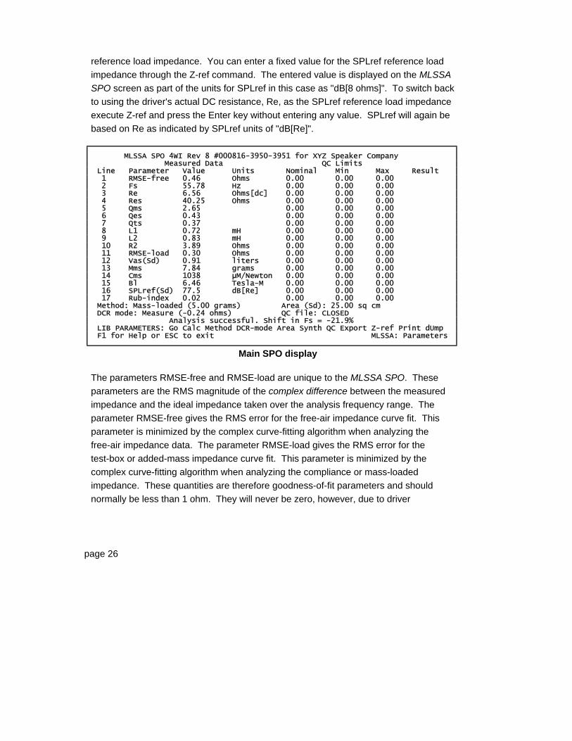
MLSSA SPO 4WI Rev 8 #000816-3950-3951 for XYZ Speaker Company Measured Data QC Limits Line Parameter Value Units Nominal Min Max Result 1 RMSE-free 0.46 Ohms 0.00 0.00 0.00 2 Fs 55.78 Hz 0.00 0.00 0.00 3 Re 6.56 Ohms[dc] 0.00 0.00 0.00 4 Res 40.25 Ohms 0.00 0.00 0.00 5 Qms 2.65 0.00 0.00 0.00 6 Qes 0.43 0.00 0.00 0.00 7 Qts 0.37 0.00 0.00 0.00 8 L1 0.72 mH 0.00 0.00 0.00 9 L2 0.83 mH 0.00 0.00 0.00 10 R2 3.89 Ohms 0.00 0.00 0.00 11 RMSE-load 0.30 Ohms 0.00 0.00 0.00 12 Vas(Sd) 0.91 liters 0.00 0.00 0.00 13 Mms 7.84 grams 0.00 0.00 0.00 14 Cms 1038 µM/Newton 0.00 0.00 0.00 15 Bl 6.46 Tesla-M 0.00 0.00 0.00 16 SPLref(Sd) 77.5 dB[Re] 0.00 0.00 0.00 17 Rub-index 0.02 0.00 0.00 0.00 Method: Mass-loaded (5.00 grams) Area (Sd): 25.00 sq cm DCR mode: Measure (-0.24 ohms) QC file: CLOSED Analysis successful. Shift in Fs = -21.9% LIB PARAMETERS: Go Calc Method DCR-mode Area Synth QC Export Z-ref Print dUmp F1 for Help or ESC to exit MLSSA: Parameters

Main SPO display

The parameters RMSE-free and RMSE-load are unique to the MLSSA SPO. These parameters are the RMS magnitude of the complex difference between the measured impedance and the ideal impedance taken over the analysis frequency range. The parameter RMSE-free gives the RMS error for the free-air impedance curve fit. This parameter is minimized by the complex curve-fitting algorithm when analyzing the free-air impedance data. The parameter RMSE-load gives the RMS error for the test-box or added-mass impedance curve fit. This parameter is minimized by the complex curve-fitting algorithm when analyzing the compliance or mass-loaded impedance. These quantities are therefore goodness-of-fit parameters and should normally be less than 1 ohm. They will never be zero, however, due to driver

page 26

Reference

nonlinearities and noise. If the noise level is low, as is usual, then these parameters indicate the degree of non-ideal behavior of the driver. If RMSE-free or RMSE-load parameters are greater than 1 ohm under low noise conditions, this probably indicates a driver problem or possibly an error in the measurement procedure. For example, in the Fixed DCR mode, the operator measures the driver DC resistance with a DVM and enters the value into SPO. If there is then an operator error measuring or entering the driver DC resistance, the 3D curve fit will be poor as it is forced to pass through an invalid data point at DC. In such cases, the values of RMSE-free and RMSE-load will increase noticeably. Similarly, the curve fit could also be degraded if the DC resistance of the test leads was is not properly account for via the DCR-mode Calibrate Manual command.

The Rub-index parameter is also unique to SPO. This unitless parameter is a measure of impedance roughness near Fs and is a very sensitive indicator of voice coil rub problems including those caused by debris being lodged in the air gap. This parameter will typically be very small (less than 0.5) on good drivers but become very large (greater than 3.0) when a driver exhibits rubbing behavior. The proper pass/fail threshold for the Rub-index parameter should be determined experimentally for each driver design. Note that when the added-mass or closed-box method is selected, the Rub-index is based on worst-case impedance curve. That is, the Rub-index is computed for both the free-air and the loaded impedance measurements but only the higher Rub-index value is actually displayed on the SPO screen. Note also that the Rub-index cannot be expected to detect all types of buzz noises. Certain types of buzz noises typically require a human listener for consistent detection.


3.5 Closed-box Method

The closed-box method is one method for determining parameters 11-16. In this method, the driver's inherent compliance is intentionally lowered (stiffness is increased) by mounting it on a sealed test box of known volume. The test box should be air tight and unlined (i.e. have no acoustic absorbing materials inside). The volume of the test box should be between 1.0 and 0.5 times the expected acoustic compliance, Vas, of the driver to be measured. Larger test box volumes will work in principle but may not cause a large enough change in the driver's resonant frequency for acceptable accuracy. SPO will not attempt to compute parameters 11-16 if the shift in Fs does not exceed 20%. Note that any air leakage through the test box, driver cone or through the interface between the driver face and the test box will invalidate the closed-box method. If leakage is suspected, try using the added-mass method, which is not subject to leakage errors.

For highest accuracy using the closed-box method, you should account for the volume of the mounting hole in your test box as well as the volume enclosed by the driver cone. The driver should be mounted to the test box with its magnet assembly located outside of the test the box to facilitate these corrections. The opening hole into the test box should have a diameter large enough to completely clear the driver’s surround but still small enough to ensure a good seal to the driver’s mounting face. The volume added by the mounting hole is simply the volume of a cylinder, which is calculated as the product of the area of the mounting hole times the thickness of the box material. To this must also be added the enclosed volume of the frustum of a cone formed between the driver’s opening face and its dust cap. This cone frustum volume can be calculated according to:

( )COCOcone SSSShV ++= 31

In this equation, So is the area of the driver’s cone. The value of So is calculated from a measurement of the cone diameter that excludes the entire surround. (Note the driver’s piston area, Sd, normally includes 1/3 of the surround.) Sc is the area of the driver’s dust cap, which is calculated from a measurement of the dust cap’s diameter. Finally, h is the depth of the dust cap as measured relative to opening face of the driver.

page 28

Reference

The value of h can be found by placing a flat reference, such as a ruler, across the face of the driver. Next, use calipers to measure perpendicular from the bottom of this reference surface down to the top of dust cap. It is suggested that all linear measurements be in centimeters with the result that the calculated volume will be in units of cubic centimeters (cc). Multiplying the result by 1000 yields liters. In summary, the total effective volume of the test box is the sum of the basic internal test box volume plus the volume of the mounting hole plus the volume enclosed between the driver’s opening face and its dust cap. Enter this total effective volume of your test box into the Method Box-loaded command to ensure the highest degree of accuracy using the closed-box method.

The driver’s effective piston area, Sd, is normally obtained from a cone diameter measurement that includes 1/3 of the surround. This is done to compensate for the fact that not all parts of surround material move in tandem with the cone. The closed-box method determines Vas and SPLref directly from the measured impedance and effective test box volume but without needing to know the driver's piston area (Sd). The piston area is needed, however, to determine Mms, Cms and Bl and so these parameters will be uncertain to the extent that the driver's piston area is uncertain. Parameters dependent on Sd are indicated when "(Sd)" is appended to the parameter symbol. When the closed-box method is used, the software will display Mms(Sd), Cms(Sd) and Bl(Sd) to indicate that these parameters are dependent on the value of Sd as entered. If the entered value of Sd is zero then Mms, Cms and Bl will not be computed. See Appendix B for the equations used to solve for parameters 11-16 using the closed-box method.

SPO normally displays and inputs mass in units of grams and volume in units of liters. When measuring very small drivers, you can elect to change to units of milligrams (mg) for mass and milliliters (ml) for volume. Note that 1 ml equals 1 cubic centimeter (cc). Units are changed though the Method Units command. The Small option selects units of mg for mass and ml for volume while the Large option selects units of grams for mass and units of liters for volume.

You select the closed-box method through the Method Box-loaded command. You will then be prompted to enter the total effective volume of your test box in liters or ml as


required. For highest accuracy, remember to account for the added volume of the mounting hole of the test box as well as the volume enclosed by the driver cone as discussed in detail above. Note that the software remembers the method and test box volume between MLSSA sessions so that you need only enter the effective test box volume once for a given test box and driver design.

The piston area is normally obtained from a cone diameter measurement that includes only 1/3 of the surround. The resulting area is entered through the Area command in square centimeters. If the measured diameter in centimeters is entered as a negative number in the Area command, SPO will automatically compute the area, Sd, from it. Alternatively, Sd can be determined indirectly as described in section 3.8 titled “Indirect Measurement of Sd”. If the piston area entered is zero then those parameters dependent upon Sd will not be calculated or displayed.

SPO assumes the free-air impedance is stored as an overlay and the box-loaded impedance is stored as the main frequency-domain trace. The parameters are then calculated through the Calc command from the Library Parameters menu. Only those impedance points framed by the marker and cursor are used in the curve fitting analysis.

The analysis frequency range should extend from the lowest available frequency to a frequency at least four times the impedance valley frequency. Otherwise, the curve-fitting algorithm may become unstable and give invalid results. If SPO determines that this condition is not met, the parameter calculations will be aborted and the error message “Insufficient HF impedance data included in analysis window: ” will be displayed followed by the analysis window frequency range used.

If you do not store the free-air impedance as an overlay and do not make the second box-loaded measurement, you can still determine the parameters numbered 1-10. If no overlay is present, SPO assumes that the main trace contains the free-air impedance and will compute and display only parameters 1-10 and parameter 17. Otherwise, it assumes the overlay contains the free-air impedance and the main trace contains the compliance-loaded impedance. If you wish only to analyze the free-air impedance, be sure to free any previously stored overlay using the Overlay Free command.

page 30

Reference

Executing Library Parameters accesses the SPO menu. Executing the Calc command computes and displays the parameters based on the current main and overlay data stored in the frequency domain. There is no need to return to the frequency domain menu to make further parameter measurements. Executing the Go command from the Library Parameters menu initiates a complete measurement-calculate-display cycle. The software automatically makes the free-air impedance measurement, stores it as an overlay, prompts you to mount the driver on the test box, makes the second impedance measurement and finally computes the parameters.

As an alternative to pressing a key after mounting the driver on a test box, you can connect a push-button switch between J4 pin-5 and J4 pin-4 (digital ground). Then you momentarily press this switch to perform the second impedance measurement.

When an RCAI is connected, connect the push-button switch between pins 5 and 4 of the TURNTABLE connector located on the front panel of the RCAI.

WARNING: Applying more than 5 volts to J4 pin-5 could result in damage to the board. For static discharge protection, you should connect a 5.1-volt zener diode across the switch. Connect its anode to digital ground and the cathode to the TTL input side. This arrangement serves to clamp any stray voltage between -0.6 and +5.1 volts to prevent static damage.


3.6 Added-mass Method

The added-mass method is another method for determining parameters 11-16. In this method the driver's total moving mass, Mms, is intentionally increased by mounting a known mass onto the driver's cone. Typically, a small amount of sticky modeling clay or Mortite (available at any hardware store) is used for this purpose. An effective alternative is to use two small but powerful "refrigerator" magnets positioned on opposite sides of the cone near the dust cap. When the magnets are brought together, they will attract each other and clamp themselves to the cone. The weight of the clay or magnets should be large enough to produce a 20% change in the driver's resonant frequency Fs. Typical values of the test mass should lie near the expected moving mass, Mms, of the driver to be measured.


The main advantage of the added-mass method is that it is not subject to leakage errors. The main disadvantage is that the act of attaching the test mass, especially clay or Mortite, will typically shift the driver compliance due to suspension hysteresis, also known as creep. Compliance shifts of up to 10% are not uncommon. The shift occurs because the cone position is usually displaced somewhat in the act of attaching the test mass. This effect is less of a problem when using two magnets as opposed to clay because the magnets can usually be attached with little disturbance to the suspension. Using an improved algorithm [10], SPO compensates for any compliance shift that occurs when attaching the test mass. The resulting measured compliance parameters (Cms and Vas) will be those that existed prior to attaching the test mass. Because of unintentional compliance changes, compliance measurements using the added mass method are not as repeatable as those using the closed box method. Nevertheless, the MLSSA SPO will yield accurate results for the other (non-compliance) parameters even in the presence of a compliance shift. In contrast, the traditional added-mass method

page 32

Reference

may yield erroneous results for the non-compliance parameters, especially Bl, if there was any compliance shift caused by attaching the test mass.

The added-mass method determines Mms, Cms and Bl directly from the measured impedance without knowledge of the driver's piston area (Sd). The piston area is needed, however, to determine Vas and SPLref so those parameters will be uncertain to the extent that the driver's piston area is uncertain. Parameters dependent on Sd are indicated when "(Sd)" is appended to the parameter symbol. When the added-mass method is used, the software will display Vas(Sd) and SPLref(Sd) to indicate that these parameters are dependent on the value of Sd as entered. If the entered value of Sd is zero then Vas and SPLref will not be computed. See Appendix B for the equations used to solve for the parameters 11-16 using the added-mass method.

You select the added-mass method through the Method Mass-loaded command. You will then be prompted to enter the test mass in grams or mg as required. Note that the software remembers the method and test mass between MLSSA sessions so that you need only enter the test mass once.

The piston area is normally obtained from a cone diameter measurement that includes only 1/3 of the surround. The resulting area is entered through the Area command in square centimeters. If the measured diameter in centimeters is entered as a negative number in the Area command, SPO will automatically compute the area, Sd, from it. Alternatively, Sd can be determined indirectly as described in section 3.8 titled “Indirect Measurement of Sd”. If the piston area entered is zero then those parameters dependent upon Sd will not be calculated or displayed.

SPO assumes the free-air impedance is stored as an overlay and the mass-loaded impedance is stored as the main frequency-domain trace. The parameters can then be calculated through the Calc command from the Library Parameters menu. Only those impedance points framed by the marker and cursor are used in the analysis.

The analysis frequency range should extend from the lowest available frequency to at least four times the impedance valley frequency. Otherwise, the curve-fitting algorithm may become unstable and give invalid results. If SPO determines that this condition is


not met, the parameter calculations will be aborted and the error message “Insufficient HF impedance data included in analysis window: ” will be displayed followed by the analysis window frequency range used.

If you do not store the free-air impedance as an overlay and do not make the second mass-loaded measurement, you can still determine the parameters numbered 1-10. If no overlay is present, SPO assumes that the main trace contains the free-air impedance and will compute and display parameters 1-10 and parameter 17. Otherwise, it assumes the overlay contains the free-air impedance and the main trace contains the mass-loaded impedance. If you wish to analyze only the free-air impedance, be sure to free any previously stored overlay using the Overlay Free command.

Executing Library Parameters accesses the SPO menu. Executing the Calc command computes and displays the parameters based on the current main and overlay data stored in the frequency domain. There is no need to return to the frequency domain menu to make further parameter measurements. Executing the Go command from the Library Parameters menu initiates a complete measurement-calculate-display cycle. The software automatically makes the free-air impedance measurement, stores it as an overlay, prompts you to attach the test mass, makes the second impedance measurement and finally computes the parameters.

As an alternative to pressing a key after attaching the test mass, you can connect a push-button switch between J4 pin-5 and J4 pin-4 (digital ground). Then you momentarily press this switch to perform the second impedance measurement.



page 34

Reference

3.7 Fixed-Mmd Method

A disadvantage of both the closed-box and added-mass methods is the need to make two separate impedance measurements under two different conditions. An alternative method that does not require two impedance measurements is the Fixed-Mmd method. The driver's moving mass exclusive of the air load, denoted Mmd, can generally be determined by other procedures such as weighing the cone assembly prior to mounting. Accurate knowledge of the driver's moving mass thus eliminates the need to take two impedance measurements and therefore permits more rapid throughput.


The Fixed-Mmd method requires knowledge of the driver's piston area (Sd) to determine Vas, Mms, Cms, Bl and SPLref so these parameters will be uncertain to the extent that the driver's piston area is uncertain. Parameters dependent on Sd are indicated when "(Sd)" is appended to the parameter's name. When the Fixed-Mmd method is used, the software will display Vas(Sd), Mms(Sd), Cms(Sd), Bl(Sd) and SPLref(Sd) to indicate that these parameters are dependent on the value of Sd as entered. If the entered value of Sd is zero then Vas, Mms, Cms, Bl and SPLref will not be computed. See Appendix B for the equations used to solve for parameters 11-16 using the Fixed-Mmd method.

You select the Fixed-Mmd method through the Method Fixed-Mmd command. You will then be prompted to enter the driver's moving mass in grams or mg as required. Note that the entered value for Mmd should not include the air-load equivalent mass, which is automatically computed from Sd and added to the entered value of Mmd by the software. If you enter a value of zero for Mmd, SPO will compute and display only parameters 1 through 10.


The piston area is normally obtained from a cone diameter measurement that includes only 1/3 of the surround. The resulting area is entered through the Area command in square centimeters. If the measured diameter in centimeters is entered as a negative number in the Area command, SPO will automatically compute the area, Sd, from it. Alternatively, Sd can be determined indirectly as described in the section titled “Indirect Measurement of Sd” below. If the piston area entered is zero then those parameters dependent upon Sd will not be calculated or displayed.

When the Fixed-Mmd method is selected, SPO assumes that the free-air impedance is stored as the main trace and there is no overlay present. The parameters are calculated through the Calc command from the Library Parameters menu. If an overlay is present, the parameters will not be computed. Only those impedance points framed by the marker and cursor are used in the analysis.

The analysis frequency range should extend from the lowest available frequency to a frequency at least four times the impedance valley frequency. Otherwise, the curve-fitting algorithm may become unstable and give invalid results. If SPO determines that this condition is not met, the parameter calculations will be aborted and the error message “Insufficient HF impedance data included in analysis window: ” will be displayed followed by the analysis window frequency range used.

Executing Library Parameters accesses the SPO menu. Executing the Calc command computes and displays the parameters based on the current data stored in the frequency domain. There is no need to return to the frequency domain menu to make further parameter measurements. Executing the Go command from the Library Parameters menu initiates a complete measurement-calculate-display cycle. The software automatically makes the free-air impedance measurement, frees any previously stored overlay and computes the parameters.

page 36

Reference

3.8 Indirect Measurement of Sd

As noted elsewhere, the piston area, Sd, is needed to compute some driver parameters. While conceptually simple, measuring a driver's piston area presents practical difficulties because the surround, which attaches the cone to the driver frame, does not move as much as the cone proper. This has led to the rule-of-thumb that the cone diameter measurement should include only 1/3 of the surround. A more accurate alternative to direct measurement of Sd is an indirect method based on applying two different parameter measurement methods successively to the same driver. This technique makes use of the fact that Vas is independent of Sd for the closed-box method while Mms is independent of Sd for the added-mass method. Then the value of Sd in square centimeters can be computed as,

210

×=CP

VWMS

o

assmsd

21

2

where Ws = 2πFs, Po = 1.18 kg/m3, C = 345 m/s and where Mms in grams is measured using the added-mass method while Vas in liters is measured using the closed-box method. Once Sd is measured for a particular driver design it is not likely to vary much from one driver to the next assuming the driver's dimensional tolerances are well controlled.

SPO will perform this calculation for you when you perform the recommended procedure as follows. First, measure the driver parameters using the closed box method and then save the results through the QC Limits Copy command. Next, measure the same driver using the added mass method. The order is important here (closed-box followed by added-mass) because the added mass procedure will typically shift the driver compliance somewhat (see Added-Mass Method section 3.6 above) while the closed box method will not. Finally, to compute and store the correct value for Sd, execute the Area command followed by Right arrow and Enter keys.


3.9 Quality Control Features

You can optionally program QC limits for some or all parameters using the QC Limits Define command. After the QC limits have been defined, they should be saved to a file using the QC Limits Save command. Then they can be reloaded later using the QC Limits Load command. After the QC limits have been entered or loaded from disk, SPO will give a pass/fail result for each parameter during a Calc or Go cycle.

You do not need to enter QC limits for all parameters; only those you wish to check. Normally, in the QC Limits Define command, the pass/fail result depends only upon the "min" and "max" QC limits fields while the "nominal" field is only for reference. By entering the "min" value as a negative number you can cause that number to be interpreted as a percentage deviation from the nominal value and then when a positive value is entered in the "max" field it will be also interpreted as a percentage deviation from nominal (e.g. 6 ohms, -5.0%, +4%). Of course, if you choose this option be aware that changing the nominal value will have a direct effect on the QC PASS/FAIL results. Also note you can choose this "percentage of nominal" option on a line-by-line basis meaning, for example, that Re could be checked in absolute ohms while Qms is checked on a percentage basis.

Note that there are no units defined for QC limits. If you change units for volume and mass through the Method Units command, the current QC limits for Mms and Vas will no longer be valid. You will need to manually change the QC limits for parameters Mms and Vas when changing from Large to Small or, from Small to Large units.

The QC Display Blank command prevents the measured parameter and QC-limits data from being displayed. Instead, a simple pass/fail result is displayed in large letters in the center of the screen after each cycle. In addition, for even greater visibility, a passed result is framed by a broad green bar while a failed result is framed by a broad red bar. This is to assure visibility of pass/fail results at a considerable distance from the computer monitor. The QC Display Unblank command reverses this action and displays the normal SPO screen.

page 38

Reference

The QC Limits Copy command copies the current measured parameters into the nominal field of the QC limits. This command is useful for temporarily saving a set of measured parameters for comparison purposes with other measurements.

The QC Limits Zero command clears all the QC limits to zero.

The QC Limits Info command displays the comment, if any, associated with the currently loaded QC-limits file.

The QC Header command allows you to enter a character string, up to 60 characters in length, which will thereafter be displayed at the top of the SPO screen. When first entered, SPO displays the software version, the software serial number and the licensed user’s name at the top of the SPO screen. The string you enter can be used to customize SPO printouts to be attached to tested driver units. For example, custom drivers tested for a particular customer can be shipped with parameter printouts that display that customer's name. To resume displaying the software version, software serial number and the licensed user’s name, execute the QC Header command and press the Enter key without entering any characters.

The QC Title command allows you to display a title string just above the measured parameters. Typically, the title string would be the driver make and model being tested but you can enter any string up to 34 characters in length.

The QC File Open command opens a QC file for automatic logging of the measured parameters during each Calc or Go cycle. QC files are plain text files. In addition to the measured parameters, the pass/fail result, time/date stamp, serial number and an optional comment are also logged to the QC file during each Go or Calc cycle. You can enter the serial numbers manually or have the software generate them automatically. Pressing the Esc key at the "QC comment:" prompt will abort a QC save operation for that particular driver. This allows you to repeat a questionable measurement without recording possibly erroneous data. The QC File Close command closes an open QC file and measurement data is no longer logged to it. A closed QC file can also be reopened later for appending with new data. The QC File List command lists the contents of any QC file.


The QC Statistics command accesses the statistical analysis features of SPO. The QC Statistics Calc command computes statistics on any previously created QC file. The QC Statistics QC-file command specifies which QC file is to analyzed. The software computes mean, standard deviation, minimum and maximum values for each parameter. Additionally, if a QC-limits file is specified through the QC Statistics Limits-file command, the software will also compute the number of failures for each parameter and the overall yield. Note that these pass/fail statistics are based on the present QC-limits file and not upon the pass/fail results logged into the QC file. This allows easy what-if experimentation using different QC limits. To get the same pass/fail results as recorded in the QC file simply specify the same QC-limits file you used during the measurement session. This QC-limits file, if any, is always recorded near the beginning of the QC file when it was opened for the first time.

MLSSA SPO QC Statistics Summary Line Parameter Units Mean STD Low High Failures 1 RMSE-free Ohms 0 0 0 0 0 2 Fs Hz 0 0 0 0 0 3 Re Ohms 0 0 0 0 0 4 Res Ohms 0 0 0 0 0 5 Qms 0 0 0 0 0 6 Qes 0 0 0 0 0 7 Qts 0 0 0 0 0 8 L1 mH 0 0 0 0 0 9 L2 mH 0 0 0 0 0 10 R2 Ohms 0 0 0 0 0 11 RMSE-load Ohms 0 0 0 0 0 12 Vas liters 0 0 0 0 0 13 Mms grams 0 0 0 0 0 14 Cms µM/Newton 0 0 0 0 0 15 Bl Tesla-M 0 0 0 0 0 16 SPLref dB 0 0 0 0 0 17 Rub-index 0 0 0 0 0 Total: 0 units QC file: Yield: Limits file: NONE LIB PARAMETERS QC STATISTICS: Calculate QC-file Limits-file Mode Print dUmp F1 for Help or ESC to exit MLSSA: Parameters

SPO Statistics screen

The QC Statistics Mode command selects between All drivers and Passed-only drivers. The All option means the statistics are computed based on all the data in the QC file regardless of the pass/fail status of the drivers. The Passed-only option means that the

page 40

Reference

statistics are calculated based only on those drivers that pass the limits defined by the current QC-limits file the failed driver data being ignored.

The QC Macro menu allows you to record, load and execute macros without returning to the normal frequency domain menu. In addition, a filename or other string can be entered during macro execution if Ctrl-u is typed in as a placeholder during macro record. See the MLSSA Reference Manual for more information regarding macros.


3.10 Exporting Parameters

The Export command will export the currently displayed parameters to a plain text file for importing into CAD packages. Also exported are the method (including the test box volume or test mass), the piston area Sd, the DCR-mode, the series resistance, the stimulus level, the MLSSA setup file used to make the impedance measurements as well as other useful data.

SPO screens contain text data although normally they are displayed in graphics video mode. The text data can be exported using the Alt-4 capture utility but first you must press Esc to temporarily return to the frequency domain and press Alt-9 to switch MLSSA into Character mode. By first switching to Character mode and then executing Library Parameters and recalculating the parameters or statistics screens, you can then press Alt-4 to export them to plain text files. Returning to the frequency domain and pressing Alt-9 again restores graphics mode. Without first switching to Character mode the Alt-4 command will capture all SPO screens as graphics data and save them to PCX files.

page 42

Reference

3.11 Synthesizing Driver Impedance

The Synthesize commands allow you to generate the ideal free-air impedance of a driver from a given set of parameters. The Synthesize Measured command uses the measured parameters for this purpose while the Synthesize Nominal command uses the parameters displayed in the "nominal" field of the QC limits. These commands are useful for studying how actual driver impedance deviates from the ideal impedance. The resulting synthesized impedance is output to a normal MLSSA binary frequency-domain FRQ data file. You can load this synthesized impedance FRQ file just like any other FRQ file to make comparisons with the actual measured impedance using overlays.

You can also determine the complex error between the ideal free-air impedance and the measured impedance as follows:

1) After measuring the parameters, create a synthetic impedance file through the Synthesize Measured command. Press Esc to return to the frequency domain.

2) Save the free-air impedance measurement data to a file by executing Transfer Save (or Overlay sAve following Box-loaded or Mass-loaded SPO measurements since the overlay will contain the free-air impedance data) and answer Y (yes) to the option to equalize the impedance data to the Main reference before saving (important).

3) Execute the Library Operations Frequency-files Difference Complex command. Enter the measured impedance filename followed by the synthesized impedance filename, followed by an output filename to store the complex error curve.

4) Execute the Transfer Load command to load the error file you just created. Note that this error is complex, including both a real part and an imaginary part. Use View Real and View Imaginary to see the real and imaginary parts of the complex impedance error. Use View Magnitude Linear to see the error magnitude. Press Alt-r to compute the RMS value of the error magnitude over the same frequency ranged you used to measure the parameters. This number should agree with the RMSE-free parameter displayed by SPO.


Procedures

4. Procedures

4.1 Direct Measurement Procedure

MLSSA can measure driver impedance without a power amplifier by using a Y-adaptor having two RCA phono plugs connected to a common RCA phono jack. You connect one plug of the Y-adaptor into the MLSSA white-MLS output (J3) and the other plug into the MLSSA input (J2), thus forming a loopback connection. The common phono jack at the other end of the Y-adaptor connects to the driver to be measured. Test clips are available with a female BNC termination. By attaching a phono-jack-to-male-BNC adaptor to the BNC-terminated test clips, you can easily connect them to the common end of the Y-adaptor using a standard audio patch cable. The cable leading to the driver under test adds series inductance which can become significant when measuring high frequency drivers or, when the cable length exceeds 1.0 meter. You can optionally measure and correct for the cable inductance in such cases.

If you have the MLSSA Remote Controlled Analog Interface (RCAI), a Y-adaptor is not required to perform direct SPO measurements. You simply plug the cable leading to the driver to be measured into the phono jack labeled SRC OUT on the rear panel of the RCAI. Note that for highest accuracy, it is suggested that you disconnect any cable currently connected to the TO IN phono jack located just below the SRC OUT connector. The two connectors are in parallel meaning that the input impedance of any power amplifier connected to the TO IN connector will be in parallel with the driver impedance.

Direct impedance measurements are recommended and preferable for several reasons. First, because the MLSSA hardware is DC coupled it is possible for SPO to measure the driver's DC resistance using the Measure DCR mode. Secondly, because no other electronics are involved, the possibility of ground loops is eliminated thus ensuring low noise measurements.


MLSSA 2000 cards contain precision 1-watt, 75.5-ohm series resistors in both the white and pink MLS outputs. These resistors are accurate to 0.1% to insure the highest possible accuracy of MLSSA impedance measurements.

WARNING: All standard setup files intended for measuring impedance assume that the series resistor is exactly 75.0 ohms. DO NOT enter 75.5 ohms into the FFT Mode Impedance command as this will result in reduced accuracy. The precision 75.5-ohm series resistors found on all on MLSSA 2000 cards are intentionally 0.5 ohm high in order to compensate for the input impedance of the MLSSA antialiasing filter, which is effectively in parallel with the 75.5-ohm series resistor.

The output current capability of MLSSA 2000 cards is 100 ma for both the pink and white outputs. This permits you to make direct SPO measurements using the maximum MLSSA output voltage of 5.23 volts, as set by the Acquisition Stimulus Amplitude command. Note that SPO measurements are best made using the normal or white MLS output on J3 (bottom phono connector).

If you do not own a MLSSA 2000 card, do not attempt to use a stimulus amplitude higher than 1 volt. Doing so, may cause current limiting in the output stage and result in erroneous impedance measurements.

Setup File Fs range Typical driver type

SPO1K.SET 15 - 30 Hz Large woofers

SPO4K.SET 30 - 100 Hz Small woofers and mid-range drivers

SPO10K.SET 100 — 300 Hz Headphone drivers, some multimedia drivers

SPO20K.SET 300 — 1000 Hz Small multimedia drivers and tweeters

Suggested setup files for various driver types

page 46

Procedures

Select a setup file appropriate to the driver you are measuring according to the table above.

Start MLSSA with setup file you selected, for example,

MLSSA SPO1K

or load the setup file through the Setup Load command.

Execute the FFT Bypass command to enter the frequency domain. Execute the Reference Go command to perform and store a reference loopback measurement. If you are using the RCAI, be sure to first execute the Acquisition Interface Drive command and select the Direct option before performing the Reference Go command. Note that the RCAI automatically disconnects the load whenever you execute the Reference Go command. Otherwise, without the RCAI, you must ensure that the test leads are open when making reference loopback measurements and then remember to re-connect them to the driver to perform actual parameter measurements.

If the length of the cable leading to the driver exceeds 1 meter or, if you are measuring high frequency drivers, it is advisable to measure and correct for the series inductance of the cable. To do this, short together the test leads and then execute the Go Once command. The impedance of the cable will be measured. Next, store this measurement as the Aux reference by executing Reference Aux Store.

Connect the test leads to the driver to be measured. Execute the Go Once command to measure the complex impedance of the driver.


Typical free-air (solid) and box-loaded (dotted) impedance curves

When using the direct method you should analyze all impedance points from the first point above DC (1 Hz for SPO1K.SET) up to the selected measurement bandwidth frequency (1000 Hz for SPO1K.SET). Note that only the impedance data windowed by the marker and cursor will be analyzed by SPO.

NOTE: The marker and cursor positions can be reversed without affecting the SPO analysis window. Therefore, the cursor could be set to the low frequency limit and the marker to the upper frequency limit, if doing so is more convenient.

The impedance valley (seen at about 150 Hz in free-air impedance curve in the figure above) should lie well below the selected measurement bandwidth frequency. If not,

page 48

Procedures

you must use a wider measurement bandwidth. Return to the time domain, execute Setup Load and load the next higher bandwidth setup file. For example, if you are using SPO1K.SET, load setup file SPO4K.SET. Press Esc to return to the time domain and execute FFT Bypass. Execute Reference Go to perform a new loopback reference measurement, being sure to first disconnect the test leads from the driver if you do not have the RCAI. Execute Go Once to re-measure the driver’s impedance, being sure to first reconnect the test leads to the driver if you do not have the RCAI.

Execute the Library Parameters command to enter the MLSSA SPO menu. Execute the Method command and select the method you wish to use. Be sure to enter the test mass weight, test box volume or the moving mass Mmd as required. If you wish to only measure parameters 1-10 using a single free-air impedance measurement, select the Fixed-Mmd method and enter zero. Refer to sections 3.5, 3.6 or 3.7 of this manual, as required, for important details regarding the Method you intend to use.

If you are measuring very small drivers, you can optionally select units of milligrams (mg) for mass and milliliters (ml) for volume through the Method Units Small command. Note that 1 ml = 1 cc.

Execute the DCR-mode command and select the Measure DCR mode. For faster but less accurate driver DC resistance measurements, you can alternatively select the Estimate option and answer ‘Y’ when asked if the signal path to the driver is DC-coupled. This selects the Estimate #1 DCR mode. Note that the Estimate #1 DCR mode is not suggested when measuring large woofers having a very low Fs as in such cases the real part of 1 Hz impedance point will no longer be a reasonable proxy for the true DC resistance.

Execute the Area command and enter the driver's area in square centimeters or, enter the diameter in centimeters as a negative number.

You are now ready to make parameter measurements. Connect the driver to the test leads and execute the Go command from the Library Parameters menu. If you had selected the Measure DCR mode, executing Go for the first time will automatically execute the DCR-mode Calibrate Auto command to calibrate SPO for accurate DC


resistance measurements as well as to measure and store the residual DC resistance of your test leads. Open the test leads when prompted then press the Enter key. SPO will measure and store the exact DC gain of the whole signal path. Next, when prompted, short your test leads together and press Enter again. SPO will measure and store the residual DC resistance of your test leads and use this value to correct all subsequent driver DC resistance measurements. Note that when the RCAI is connected, SPO will immediately perform the DC gain measurement, even if your test leads are not actually open. This is possible with the RCAI, which is able to create an open circuit condition on its own. When prompted, however, you will still need to short the test leads together manually and then press Enter to make the second measurement, which is of the DC resistance of your test leads. After DC resistance calibration is complete, SPO will prompt you to reconnect your test leads to the driver.

SPO will next measure the driver's DC resistance. Next, the driver's free-air impedance is measured and stored as an overlay. SPO will next prompt you to attach the test mass or, mount the driver on a test box, depending upon the method you selected. Press any key when ready. The second impedance measurement will then be made, the parameters calculated and the results displayed. In addition, the percentage change in Fs caused by the load is also displayed for the added-mass and closed-box methods. MLSSA SPO expects a least a -10% change in Fs for the added-mass method and at least a +20% change in Fs for the box-loaded method. If these minimums are not met, the parameter calculation will abort. Of course, if you selected the Fixed-Mmd method, only the free-air impedance is needed to compute the parameters.

page 50

Procedures

ERROR MESSAGES: The Calc and Go commands always perform a preliminary impedance scan prior to performing the 3D curve fit. The purpose of this scan is to check that the impedance data is "reasonable" to prevent possibly erroneous results. If SPO finds that the impedance data is "unreasonable”, the message "Invalid impedance data segment in analysis window: " will be displayed followed by the analysis window frequency range, as defined by the marker and cursor positions. This error can be caused by strong secondary impedance peaks. Such secondary peaks, if present, should not be included in the analysis window. If SPO senses that you are including too little HF impedance data the message "Insufficient HF impedance data included in analysis window: ” will be displayed and the measurement aborted.

As an alternative to pressing a key after attaching the test mass or mounting the driver on a test box, you can connect a push-button switch between J4 pin-5 and J4 pin-4 (digital ground). Then you momentarily press this switch to perform the second impedance measurement.



If you now open a QC file through the QC File Open command, further measurement results will be logged to it automatically. To discontinue data logging close the QC file through the QC File Close command.


Procedures

4.2 Power Amplifier Measurement Procedure

If you wish to measure the parameters at higher driver levels than are attainable using the direct method, you must use a power amplifier. Most audio power amplifiers are AC coupled. If you use an AC-coupled power amplifier, the analysis window must exclude frequencies below the amplifier's low cut-off frequency. You cannot use the Measure DCR mode with any AC-coupled power amplifier. Instead, use the Fixed DCR mode, which requires manually measuring the driver’s DC resistance with a DVM or, use the Estimate #2 DCR mode, which estimates the driver’s DC resistance from the available AC impedance data falling between the marker and the cursor. If your AC-coupled power amplifier has significant response down to 1 Hz, it may be possible to use the Estimate #1 DCR mode, which estimates the driver’s DC resistance from the real part of the lowest available AC impedance data point. However, most AC-coupled power amplifiers have significant response only down to about 10 Hz so they must be used only with the Estimate #2 or Fixed DCR modes.

Impedance measurements using a power amplifier are greatly facilitated and much safer using the MLSSA Remote Controlled Analog Interface (RCAI) which is highly recommended for this purpose. With the RCAI, high power amplifiers of up to 1 kW can be used. The RCAI contains a precision 13-dB attenuator that serves to protect MLSSA’s antialiasing filter from damage during reference measurements. The RCAI also includes a precision 75-ohm, 12-watt series resistor, which is protected from overheating via a thermal cut-off switch.

If you do not have the RCAI, the following guidelines should be followed. Use only common ground power amplifiers having relatively low output power capability. The use of high power audiophile amplifiers especially those having floating or bridged output circuits should be avoided. The high power capability of these amplifiers can result in inadvertent damage to MLSSA's antialiasing filter or, to the power amplifier. In addition, floating amplifier output circuits can result in high ground-loop currents since MLSSA's input and output circuits are single ended. Also, be sure the reference loopback measurement includes the power amplifier and that the power amplifier's output impedance is low relative to the series resistor used. A series resistance of 75


ohms is recommended. However, lower values can be used down to about 10 ohms, to increase the effective drive level for a given drive voltage.

If you do not have the RCAI, you also need to connect the selected series resistor, of suitable power rating, directly to the hot terminal of the power amplifier output. Connect the free end of the power resistor to a piece of heavy gauge wire with an alligator clip at the opposite end for connecting to the driver. Connect a second piece of heavy gauge wire, of equal length, to the ground terminal of the amplifier output with a second alligator clip for connecting to the driver. To prevent ground loops, it’s advisable to connect another piece of heavy gauge wire from ground terminal of the power amplifier to the L-bracket of the MLSSA card or, directly to the frame of the PC. Connect the hot lead of the MLSSA input (J2) to the series power resistor on the side opposite the power amplifier’s hot terminal, that is, where the series resistor and hot test lead join together. Using an audio patch cable, connect the white-MLS output (J3) to the amplifier's input and power up the amplifier.

Select a setup file appropriate for the driver you are measuring according to the following table.

Setup File Fs range Typical driver type

SPO1KPA.SET 15 - 30 Hz Large woofers

SPO4KPA.SET 30 - 100 Hz Small woofers and mid-range drivers

SPO10KPA.SET 100 — 300 Hz Headphone drivers, some multimedia drivers

SPO20KPA.SET 300 — 1000 Hz Small multimedia drivers and tweeters

Suggested setup files for various driver types

Start MLSSA with setup file you selected, for example,

MLSSA SPO1KPA

page 54

Procedures


Execute the FFT Mode command and select the Impedance option. Enter the series resistance of the out-board series resistor. For highest accuracy, it is advisable to measure this resistor with a high quality DVM.

If an RCAI is connected, there is no need to execute the FFT Mode command as the correct series test resistance of exactly 75 ohms is already entered. However, with the RCAI connected, you will need to execute Acquisition Interface Drive and select the Power-amp option.

NOTE: After entering the out-board series resistance you can save it to SPO1KPA.SET, SPO4KPA.SET, SPO10KPA.SET or SPO20KPA.SET, as appropriate, through the Setup Save command. Thereafter, there will be no need to re-enter the series resistance each time upon starting MLSSA.

Connect the test leads to the driver. Press the Del key to enable the white-MLS stimulus and then use the = key or the + key on the numeric keypad to slowly increase the stimulus level until the noise is clearly audible from the driver.

NOTE: After setting a stimulus level appropriate for your power amplifier you can save it to SPO1KPA.SET, SPO4KPA.SET, SPO10KPA.SET or SPO20KPA.SET, as appropriate, through the Setup Save command. Thereafter, there will be no need to re-adjust the stimulus level each time upon starting MLSSA.

Disconnect the driver and execute the FFT Bypass command to enter the frequency domain. Execute the Reference Go command to perform and store a reference loopback measurement. Note that the RCAI automatically disconnects the load from the SPEAKER terminals whenever you execute the Reference Go command. Otherwise, without the RCAI, you must ensure that the test leads are open when


making reference loopback measurements and then remember to re-connect them to the driver to perform actual parameter measurements.

If the length of your test leads leading to the driver exceeds 1 meter or, if you are measuring high frequency drivers, it is advisable to measure and correct for their series inductance. To do this, short together the test leads and execute the Go Once command. The impedance of the test leads will be measured. Next, store this measurement as the Aux reference by executing Reference Aux Store.

Re-connect the test leads to the driver to be measured. Execute the Go Once command to measure the complex impedance of the driver.

Selecting the analysis window with an AC-coupled power amplifier

page 56

Procedures

If you are using a DC-coupled power amplifier, the marker and cursor positions are already set to define the recommended SPO analysis window frequency range: the marker at the lowest available frequency and the cursor at the measurement bandwidth frequency, depending upon the setup file you loaded. If you are using an AC-coupled power amplifier, press F9 to place the marker at the cursor position. Next, position the cursor to the lowest frequency that does not contain an excessive amount of noise (see figure above). The impedance data will become increasingly noisy at low frequencies due to the low frequency cut-off of the power amplifier, which should lie well below the driver's resonant frequency Fs. The exact point is not critical because of the noise immunity of the analysis method. Only the impedance points windowed by the marker and cursor will be analyzed by SPO. The windowed impedance points should start from the lowest reliable frequency (12 Hz in the example above) and extend up to the selected measurement bandwidth frequency (1000 Hz for SPO1KPA.SET).

NOTE: The marker and cursor positions can be reversed without affecting the SPO analysis window. Therefore, the marker could be set to the low frequency limit and the cursor to the upper frequency limit, if doing so is more convenient.

The impedance valley (seen at about 200 Hz in the figure above) should lie well below the selected measurement bandwidth frequency. If not, you must use a wider measurement bandwidth. Return to the time domain, execute Setup Load and load the next higher bandwidth setup file. For example, if you are using SPO1KPA.SET, load setup file SPO4KPA.SET and repeat the whole procedure given above.

Execute the Library Parameters command to enter the SPO menu. Execute the Method command and select the method you wish to use. Be sure to enter the test mass weight, test box volume or the moving mass Mmd, as required. If you wish to only measure parameters 1-10 using a single free-air impedance measurement, select the Fixed-Mmd method and enter zero. Refer to sections 3.5, 3.6 or 3.7 of this manual, as required, for important details regarding the Method you intend to use.




Execute the DCR-mode command. If your power amplifier is AC coupled, select the Fixed DCR mode if the DC resistance of each driver will be measured manually using a DVM. Otherwise, choose the Estimate #2 DCR mode by answering ‘N’ when asked if the signal path is DC coupled. The Estimate #2 DCR mode estimates driver DC resistance exclusively from the AC impedance data included within the SPO analysis window. The Estimate #2 mode is not nearly as accurate as using a DVM but is much faster. The Estimate #1 mode can sometimes be used if your power amplifier is not truly DC coupled but still has significant response down to 1 Hz, that is, it has a very low cut-off frequency. The Estimate #1 DCR mode estimates the driver DC resistance from the real part of the lowest available AC impedance point, even if that point does not fall within the SPO analysis window. The Measure mode is the most accurate by far since it measures the DC resistance the same as a DVM would. Select the Measure mode only if you are certain your power amplifier frequency response truly goes all the way down to DC. Otherwise, severe DC resistance measurements will result.

Note that it is important to measure and enter the residual series resistance of your test leads using a high quality DVM when using the Fixed, Estimate #1 or Estimate #2 DCR modes. Measure the series resistance of your test leads running from the power amplifier output terminals to the test clips, excluding the out-board series resistor. Each test lead can be measured separately and the two figures added together to get the total. If using the RCAI, measure the leads running from SPEAKER terminals of the RCAI but do not include the leads running from the power amplifier to the RCAI. Each test lead can be measured separately and the two figures added together to get the total. Before measuring the test leads, short the DVM’s leads together to measure their resistance and make a note of this value to later subtract it from the measured resistance of the SPO test leads. Many DVMs have a “Relative” or similar mode that allows you to store the DVM’s test lead resistance, which is then subtract automatically

page 58

Procedures

from the DC resistance measurement of your test leads. Enter the total value of your test lead DC resistance through the DCR-mode Calibrate Manual command.

If you are in the Fixed DCR mode, use a DVM to measure the driver's DC resistance at the driver's terminals and enter it through the DCR-Mode Fixed command.

You are now ready to make parameter measurements. Connect the driver to the test leads and execute the Go command from the Library Parameters menu. If you had previously selected the Measure DCR-mode (valid only for truly DC-coupled power amplifiers), executing Go for the first time will automatically calibrate SPO for accurate DC resistance measurements as well as measure and store the residual DC resistance of your test leads. Open the test leads when prompted then press the Enter key. SPO will measure and store the exact DC gain of the whole signal path. Next, when prompted, short your test leads together and press Enter again. SPO will measure and store the residual DC resistance of your test leads and use this value to correct all subsequent measurements. Note that when the RCAI is connected, SPO will immediately perform the DC gain measurement, even if your test leads are not actually open. This is possible with the RCAI, which is able to create an open circuit condition on its own. When prompted, however, you will still need to short the test leads together manually and then press Enter to make the second measurement, which is of the DC resistance of your test leads. After DC resistance calibration is complete, SPO will prompt you to reconnect your test leads to the driver.

If you had selected the Measure DCR mode, SPO will next measure the driver's DC resistance. Next, the driver's free-air impedance is measured and stored as an overlay. SPO will next prompt you to attach the test mass or, mount the driver on a test box depending upon the method you selected. Press any key when ready. The second impedance measurement will then be made, the parameters calculated and the results displayed. In addition, the percentage change in Fs caused by the load is also displayed for the added-mass and closed-box methods. SPO expects a least a -10% change in Fs for the added-mass method and at least a +20% change in Fs for the box-loaded method. If these minimums are not met, the parameter calculation will abort. If you selected the Fixed-Mmd method, only the free-air impedance is needed to compute the parameters and no second impedance measurement is required.


ERROR MESSAGES: The Calc and Go commands always perform a preliminary impedance scan prior to performing the 3D curve fit. The purpose of this scan is to check that the impedance data is "reasonable" to prevent possibly erroneous results. If SPO finds that the impedance data is "unreasonable”, the message "Invalid impedance data segment in analysis window: " will be displayed followed by the analysis window frequency range, as defined by the marker and cursor positions. This error can be caused by strong secondary impedance peaks. Such secondary peaks, if present, should not be included in the analysis window. If MLSSA SPO senses that you are including too little HF impedance data the message "Insufficient HF impedance data included in analysis window:” will be displayed and the measurement aborted.

As an alternative to pressing a key after attaching the test mass or mounting the driver on a test box, you can connect a push-button switch between J4 pin-5 and J4 pin-4 (digital ground). Then you momentarily press this switch to perform the second impedance measurement.



If you now open a QC file through the QC File Open command, further measurements will be logged to it automatically. To discontinue data logging close the QC file through the QC File Close command.

page 60

Procedures

4.3 Acoustic Frequency Response + Parameters Procedure

Whenever MLSSA is not in the Impedance FFT mode and a MLSSA RCAI is connected, SPO automatically configures the RCAI to perform impedance measurements. For example, suppose MLSSA and the RCAI are both configured to measure speaker driver frequency response (Transfer Function FFT mode) using a microphone and the pink-MLS stimulus. Upon entering SPO via the Library Parameters command, the RCAI is automatically re-configured to measure impedance using the white-MLS. Therefore, upon entering SPO you can straight away perform driver T/S parameter measurements, even if you were previously measuring driver acoustic frequency response. Upon exiting SPO, the RCAI is restored to its original state, thus allowing you to immediately resume measuring driver frequency response or, whatever MLSSA was setup to measure prior to entering SPO.

You can set the analysis window frequency range used by SPO to be different from the current marker and cursor positions to free up the marker and cursor for other purposes, such as to define the QC PASS/FAIL frequency range for QC PASS/FAIL testing of driver acoustic frequency response. To set the SPO analysis window frequency range, first execute the Go Impedance command to measure the driver’s impedance. Next, set the marker and cursor positions for the desired SPO analysis window frequency range, and finally execute Library Parameters to enter SPO. SPO will respond with a high-pitched beep and the message: “SPO analysis window stored: ” followed by the analysis frequency range you had selected using the marker and cursor. Press Esc to return to the frequency domain. Next, execute the Go Once command to perform an acoustic frequency response or other non-impedance measurement. From that point on, you can set the marker and cursor as desired for any other purpose without affecting the SPO analysis window, as long as you enter SPO without a displayed impedance curve that was previously measured using the Go Impedance command.

Note here that when MLSSA is displaying an impedance curve loaded from disk or, even one previously measured by SPO itself, the current marker and cursor positions are ignored by SPO, thus preventing inadvertent changes to the SPO analysis window. To set a new SPO analysis window, execute Go Impedance again, set the marker and


cursor positions for the new analysis window frequency range and then enter SPO again to store the new SPO analysis window.

The FFT size needs to be large enough to ensure sufficient frequency resolution for accurate SPO measurements. The setup file LOUDS-Z.SET sets a 20 kHz measurement bandwidth and uses a 16,384-point FFT to achieve the fine frequency resolution required by SPO. Thus, setup file LOUDS-Z.SET optimally configures MLSSA for acoustic frequency response measurements up to 20 kHz, as well as for T/S parameter measurements via SPO when the RCAI is connected.

Start MLSSA with setup file LOUDS-Z.SET,

MLSSA LOUDS-Z


Unlike other setup files described elsewhere in this manual, which program the Impedance FFT mode, LOUDS-Z.SET programs the Transfer Function FFT mode. After loading this setup file, you can optionally use the FFT Mode command (from the time domain) to select the Sensitivity FFT mode to measure absolute driver sensitivity in dB-SPL/watt provided you have a calibrated microphone and preamp. You can even select another FFT mode depending upon your application but do not select the Impedance FFT mode, as SPO will automatically configure the RCAI to measure impedance whenever SPO is entered.

This procedure assumes you are using a power amplifier since one is typically required to measure driver frequency response at realistic SPL levels. A DC-coupled power amplifier is preferred allowing SPO to perform accurate measurements of the driver’s true DC resistance. If your power amplifier is AC coupled, as most are, less accurate options for estimating the driver’s DC resistance will be discussed below.

Execute Acquisition Interface Drive and select the Power-amp option.

page 62

Procedures

Connect the test leads to the driver. Press the Del key to enable the MLS stimulus and then use the = key or the + key on the numeric keypad to slowly increase the stimulus level until the MLS noise is clearly audible from the driver.

NOTE: After setting a stimulus level appropriate for your power amplifier you can save it to LOUDS-Z or another setup filename through the Setup Save command. If you had changed the FFT mode to measure Sensitivity, that change will also be saved. Thereafter, there will be no need to re-adjust the stimulus level or change the FFT mode each time upon starting MLSSA with the same setup file.

Execute the FFT Bypass command to enter the frequency domain. Execute the Reference Go command to perform and store a reference loopback measurement or your power amplifier. Note that the RCAI automatically disconnects the load from the SPEAKER terminals whenever you execute the Reference Go command.

It is suggested not to use the Aux reference to correct for the test lead inductance. Test lead inductance is generally insignificant unless the test leads are very long and the Aux reference is then free to store a frequency response measurement of a reference driver for QC PASS/FAIL test purposes. In addition, there is some possibility that you could inadvertently damage your power amplifier (see warning below).

WARNING: Do not execute Go Once with the test leads shorted as the output terminals of your power amplifier will encounter a dead short, which will most likely blow the fuse in the RCAI but could also damage your power amp. Use only the Go Impedance command to measure the residual resistance of your test leads

However, if you do have very long test leads and/or still want to correct for their series inductance, you can use the Aux reference as follows: Short your test leads together and execute Go Impedance (not Go Once) followed by Reference Aux Store. The residual series impedance of your test leads is now stored as the Aux reference and will be subtracted from all subsequent impedance measurements. Note that when the Aux


reference contains impedance data, MLSSA will not apply it to non-impedance measurements, so they will be unaffected. Similarly, when the Aux reference contains non-impedance data, MLSSA and SPO will not apply it to driver impedance measurements.

Select an appropriate SPO analysis window frequency range for the driver you are measuring according to the following table.

Analysis Window Upper Limit

Fs range Typical driver type

1 kHz 15 - 30 Hz Large woofers

4 kHz 30 - 100 Hz Small woofers and mid-range drivers

10 kHz 100 — 300 Hz Headphone drivers, some multimedia drivers

20 kHz 300 — 1000 Hz Small multimedia drivers and tweeters

Suggested analysis windows for various driver types

Execute the Go Impedance command to measure the complex impedance of the driver. Move the cursor to set the upper limit of the SPO analysis window according to the table above. For example, for small woofers move the cursor to the 4 kHz position. Press F9 to set the marker to that position. See figure below for this example.

NOTE: The marker and cursor positions can be reversed without affecting the SPO analysis window. Therefore, the marker could be set to the low frequency limit and the cursor to the upper frequency limit, if doing so is more convenient.

page 64

Procedures

Selecting the analysis window after executing Go Impedance

If you are using a DC-coupled power amplifier, press the Home key to move the cursor down to the lowest available frequency. If you are using an AC-coupled power amplifier, position the cursor to the lowest frequency that does not contain an excessive amount of noise. The impedance data will become increasingly noisy at low frequencies due to the low frequency cut-off of the power amplifier, which should lie well below the driver's resonant frequency Fs. The exact point is not critical because of the noise immunity of the analysis method. Only the impedance points framed by the marker and cursor will be analyzed by SPO.

As a double check on the suggested analysis window, the impedance valley (seen at about 300 Hz in the figure above) should lie well below the upper frequency limit of the


SPO analysis window. If not, you should choose a higher upper frequency limit for the SPO analysis window.

Execute the Library Parameters command to enter SPO. SPO will respond with a high-pitched beep and the message: “SPO analysis window stored: ” followed by the analysis frequency range you had selected using the marker and cursor. Press Esc to return to the frequency domain. Next, execute the Go Once command to perform a frequency response measurement of the driver using a microphone connected to one of the mic mux inputs of the RCAI. See MLSSA manual section 6.1 titled Loudspeaker Anechoic Response for details on measuring driver frequency response. Also, see the MLSSA RCAI manual for further details.

From this point on, you can set the marker and cursor as desired for any other purpose without affecting the SPO analysis window, as long as you enter SPO without a displayed impedance curve that was previously measured using the Go Impedance command. Note here that when MLSSA is displaying an impedance curve loaded from disk or, even one previously measured by SPO itself, the current marker and cursor positions are ignored by SPO, thus preventing inadvertent changes to the SPO analysis window. To set a new SPO analysis window, execute Go Impedance once again, set the marker and cursor positions for the new analysis window frequency range and enter SPO once again to store the new analysis window.

Execute Library Parameters to enter SPO. Execute the Method command and select the method you wish to use. Be sure to enter the test mass weight, test box volume or the moving mass Mmd as required. If you wish to only measure parameters 1-10 using a single free-air impedance measurement, select the Fixed-Mmd method and enter zero. Refer to sections 3.5, 3.6 or 3.7 of this manual, as required, for important details regarding the Method you intend to use.


page 66

Procedures


Execute the DCR-mode command. If your power amplifier is AC coupled, select the Fixed DCR mode if the DC resistance of each driver will be measured manually using a DVM. Otherwise, choose the Estimate #2 DCR mode by answering ‘N’ when asked if the signal path is DC coupled. The Estimate #2 DCR mode estimates driver DC resistance from the AC impedance data included within the SPO analysis window. The Estimate #2 mode is not nearly as accurate as using a DVM but is much faster. The Estimate #1 mode can be used if your power amplifier is not truly DC coupled but still has significant response down to 1 Hz, that is, it has a very low cut-off frequency. The Estimate #1 DCR mode estimates the driver DC resistance from the real part of the lowest available AC impedance point, even if that point does not fall within the SPO analysis window. The Measure mode is the most accurate by far since it measures the DC resistance the same as a DVM would. Select the Measure mode only if you are certain your power amplifier frequency response truly goes all the way down to DC. Otherwise, severe DC resistance measurement errors will result.

The Estimate #1 mode is not suggested for woofers even if your power amplifier goes down to 1 Hz. The reason is that when using setup file LOUDS-Z.SET the lowest available frequency is 3.7 Hz, which is too far above DC to be considered a proxy for the typical woofer’s true DC behavior. However, it is a valid proxy for DC when measuring drivers having a value of Fs above 100 Hz. When measuring woofers one possibility is to select a much lower measurement bandwidth, such as 4 kHz or lower, which will allow you to safely select the Estimate #1 DCR mode. In that case, however, you will not be able to measure the woofer’s frequency response above 4 kHz or, whatever new bandwidth setting is chosen. Note also that after changing the MLSSA measurement bandwidth via the Acquisition Bandwidth command, you will need to execute a new Reference Go command, followed by the Go Impedance command, and then move the marker and cursor as described above to redefine the SPO analysis window and finally enter SPO again to store it.

Note that it is important to measure and enter the residual series resistance of your test leads using a high quality DVM when using the Fixed, Estimate #1 or Estimate #2 DCR


modes. Measure the test leads from the SPEAKER terminals of the RCAI but do not include the leads running from the power amplifier to the RCAI. Each test lead can be measured separately and the two figures added together to get the total. Before measuring the test leads, short the DVM leads together to measure their resistance and make a note of this value to later subtract it from the measured test lead resistance. Many DVMs have a “Relative” or similar mode that allows you to store the DVM’s test lead resistance, which is then subtract automatically from the DC resistance measurement of your test leads. Enter the total value of your test lead DC resistance through the DCR-mode Calibrate Manual command.

If you have selected the Fixed DCR mode, use a DVM to measure the driver's DC resistance taken right at the driver's terminals and enter this value through the DCR-Mode Fixed command.

You are now ready to make parameter measurements. If necessary, reconnect the test leads to the SPEAKER terminals of the RCAI and reconnect the driver to the other end of your test leads. Execute the Go command from the Library Parameters menu. If you had previously selected the Measure DCR-mode (valid only for truly DC-coupled power amplifiers), executing Go for the first time will automatically calibrate SPO for accurate DC resistance measurements as well as measure and store the residual DC resistance of your test leads. SPO will measure and store the exact DC gain of the whole signal path. Next, when prompted, short your test leads together and press the Enter key. SPO will measure and store the residual DC resistance of your test leads and use this value to correct all subsequent measurements. After DC resistance calibration is complete, SPO will prompt you to reconnect your test leads to the driver.

If you had selected the Measure DCR mode, SPO will next measure the driver's DC resistance. Next, the driver's free-air impedance is measured and stored as an overlay. SPO will next prompt you to attach the test mass or, mount the driver on a test box depending upon the method you selected. Press any key when ready. The second impedance measurement will then be made, the parameters calculated and the results displayed. In addition, the percentage change in Fs caused by the load is also displayed for the added-mass and closed-box methods. SPO expects a least a -10% change in Fs for the added-mass method and at least a +20% change in Fs for the

page 68

Procedures

box-loaded method. If these minimums are not met, the parameter calculation will abort. If you had previously selected the Fixed-Mmd method, only the free-air impedance is needed to compute the parameters and no second impedance measurement is required.

ERROR MESSAGES: The Calc and Go commands always perform a preliminary impedance scan prior to performing the 3D curve fit. The purpose of this scan is to check that the impedance data is "reasonable" to prevent possibly erroneous results. If SPO finds that the impedance data is "unreasonable”, the message "Invalid impedance data segment in analysis window: " will be displayed followed by the analysis window frequency range. This error can be caused by strong secondary impedance peaks. Such secondary peaks, if present, should not be included in the analysis window. If SPO senses that you are including too little HF impedance data the message "Insufficient HF impedance data included in analysis window:” will be displayed and the measurement aborted.

As an alternative to pressing a key after attaching the test mass or mounting the driver on a test box, you can connect a push-button switch between pins 4 and 5 of the TURNTABLE connector located on the front panel of the RCAI. Then you momentarily press this switch to perform the second impedance measurement.

If you now open a QC file through the QC File Open command, further measurements will be logged to it automatically. To discontinue data logging close the QC file through the QC File Close command.

Press the Esc key to return to the frequency domain. Execute the Go Once command to measure the frequency response of same driver. You can now use all of the QC PASS/FAIL features described in detail in the MLSSA manual section 3.39 titled QC PASS/FAIL Functions. You are also now free to set the marker and cursor positions, as required, to define frequency range used by the QC-limits Compare and QC-limits Go commands. If you again enter SPO via the Library Parameters command, the SPO analysis window you had previously defined will still be in effect thus allowing you to again measure the driver T/S parameters straight away using the Go command. Of


course, you can also use the T/S parameter QC PASS/FAIL functions built into SPO. After pressing Esc to exit SPO, you can immediately execute QC-limits Go Once, as the marker and cursor positions will be then same as they were when had last you entered SPO.

Note that if the driver is mounted inside a small enclosure or to a test baffle, the measured parameters will be affected somewhat by the proximity of the driver to these structures. Therefore, the measured parameters may differ slightly from what they would measure in free air. However, for production QC purposes absolute parameter accuracy is not important since measurements are often only compared relative to a known good driver that was previously measured using the same mounting arrangement.

page 70

Procedures

4.4 Production QC Tips

When using MLSSA SPO for production QC the following guidelines are recommended.

1) Perform a new loopback reference measurement at the start of each working day after allowing a 10-minute warm-up period.

Reference measurements correct for antialiasing filter error as well as power amplifier gain errors if a power amplifier is used. Since both are electronic devices, they can drift over time and temperature. It therefore makes sense to perform a new loopback reference measurement at the start of each working day after a 10-minute warm-up period to allow internal computer and amplifier temperatures to stabilize. While MLSSA does allow you to save a reference measurement to a file and reload it later, this is not recommended because the saved reference data will gradually become increasingly stale due to long-term drift and seasonal temperature changes.

2) Make sure MLSSA SPO is completely set up and ready to go before opening a QC file for data logging.

When a new QC file is opened or an existing one is opened for overwriting, a new header is created at the beginning of the QC file which stores a host of important information including the current method, test mass or test box volume, DCR mode, driver cone area, stimulus level, QC-limits filename and QC title. Therefore, if you open a QC file and then go back and change one of these setup parameters, the setup data recorded in the QC file header will no longer be current. In addition, it's a good idea to complete at least one dry run measurement sequence before opening a QC file for data logging.

3) Use macros to streamline production testing.

If you intended to have non-technical line personnel setup and operate SPO, macros can be created to reduce operational complexity. Thus, for instance, you might create a simple macro which guides the operator through the steps needed to perform a loopback reference measurement. If you save this macro to a file named ALT-F1.MAC,


the operator need only press the Alt-F1 key combination at the start of each day to perform the reference measurement

4) Use bar-codes to track serial numbers.

Several PC-based bar-code readers are currently available. One type called a wedge device connects between the keyboard and computer. This arrangement allows serial numbers read from bar codes to be inserted in the same way as characters typed on the keyboard. To use a wedge-type bar-code reader with the SPO make sure you select the manual entry of serial numbers option when you open a QC file.

page 72

Bibliography

5. Bibliography

1. A.N. Thiele, "Loudspeakers in Vented Boxes", Journal of the Audio Engineering Society (JAES), vol. 19, pp 382-392 (May 1971) and pp 471-483 (June 1971).

2. R.H. Small, "Direct-Radiator Loudspeaker System Analysis" JAES, Vol. 20, No. 5, pp 383-395, 1972 June.

3. L.L. Beranek, Acoustics, 1986 Edition, Published for the Acoustical Society of America by the American Institute of Physics.

4. A.J.M. Kaizer, "Modeling of the Nonlinear Response of an Electrodynamic Loudspeaker by a Volterra Series Expansion" JAES, Vol. 35, No. 6, pp 421-433, 1987 June. (See Figure 2)

5. D.R. Birt, "Nonlinearities in Moving-Coil Loudspeakers with Overhung Voice Coils" JAES, Vol. 39, No. 4, pp 219-231, 1991 April.

6. J. Vanderkooy, "A Model of Loudspeaker Driver Impedance Incorporating Eddy Currents in the Pole Structure" JAES, Vol. 37, No. 3, pp 119-128, 1989 March.

7. J.R. Wright, "An Empirical Model for Loudspeaker Motor Impedance" JAES, Vol. 38, No. 10, pp 749-754, 1990 October.

8. W.M. Leach, R.W. Schafer, T.P. Barnwell, "Time-Domain Measurements of Loudspeaker Driver Parameters" IEEE Transactions on Acoustics, Speech and Signal Processing, Vol. ASSP-27, No. 6, pp 734-739, 1979 December.

9. Dick Campbell, "MLSSA vs. Sine Testing: A Tutorial on Methodology" Speaker Builder, Vol. 13, No. 1, pp 26-34, One/1992.

10. R.H. Small, Private communication


Menus

Appendix A Menu Trees

LIB PARAMETERS │ ├─ GO (initiates measure-calculate cycle) ├─ CALC (calculates parameters) ├─ METHOD │ │ │ ├─ BOX-LOADED: Enter box size in liters │ ├─ MASS-LOADED: Enter mass in grams │ ├─ FIXED-MMD: Enter moving mass in grams │ └─ UNITS: Small Large │ ├─ DCR-MODE │ │ │ ├─ FIXED: Enter driver DCR in ohms │ ├─ MEASURE │ ├─ ESTIMATE │ └─ CALIBRATE: Auto Manual │ ├─ AREA: Enter piston area in square cm │ ├─ SYNTHESIZE │ │ │ ├─ MEASURED: (uses measured parameters) │ └─ NOMINAL: (uses nominal parameters) │ ├─ EXPORT: Enter text filename ├─ Z-REF: Enter load impedance in ohms ├─ PRINT ├─ DUMP │ └─ QC │ ├─ TITLE: Enter title string ├─ HEADER: Enter header string ├─ DISPLAY: Blank Unblank ├─ FILE: Open Close List │


│ ├─ LIMITS │ │ │ ├─ DEFINE: Enter QC limits data │ ├─ COPY (Copies parms to nominal field) │ ├─ ZERO (Clears all QC limits) │ ├─ LOAD: Enter filename to load │ ├─ SAVE: Enter filename to save │ └─ INFO: (Displays QC-limits file comment) │ ├─ STATISTICS │ │ │ ├─ CALCULATE (calculates statistics) │ ├─ QC-FILE: Enter QC-file to analyze │ ├─ LIMITS-FILE: Enter QC limits file │ ├─ MODE: All Passed-only │ ├─ PRINT │ └─ DUMP │ └─ MACRO ├─ EXECUTE (executes current macro) ├─ DEBUG: Enable Disable ├─ LOAD: Enter filename to load ├─ SAVE: Enter filename to save ├─ INFO: (displays info about macro) ├─ FREE (frees macro buffer storage) ├─ VARIABLE: ctrl-V ctrl-W ctrl-X ctrl-Y ctl-Z └─ COMMAND ├─ PAUSE ├─ DELAY ├─ BEEP ├─ MESSAGE ├─ RUN ├─ SIGNAL ├─ WAIT ├─ EXEC ├─ IF-PASSED-QC: Execute Signal ├─ IF-FAILED-QC: Alarm Execute Signal ├─ MARK (mark return for LOOP) └─ LOOP (enter loop repetitions)

page 76

Equations

Appendix B Equations

Symbol definitions and units

Bl = driver transduction constant in Tesla-meters

C = 345 m/s speed of sound in air

Cms = mechanical compliance in meters/Newton

Mms = moving mass including air load in kilograms

Mmd = moving mass excluding air load in kilograms

Qes = electrical Q in free air

Qms = mechanical Q in free air

Qts = total Q in free air

Qect = electrical Q of loaded driver

Re = DC resistance of voice coil in ohms

Res = resistance due to mechanical losses in ohms

Sd = piston area in m2

Po = 1.18 kg/m3 density of air

Mt = added mass test load in kilograms

Vt = closed box test volume in m3

Ws = resonant frequency in free air in rad/sec

Wct = resonant frequency of loaded driver in rad/sec

SPLref = driver efficiency expressed as dB-SPL/watt

Zref = reference load impedance for SPLref


Electrical Q and total Q equations

es

emses R

RQQ =

mses

msests QQ

QQQ

+=

Equations for closed-box method

−= 1

ess

ectcttas QW

QWVV

22do

asms SCP

VC =

mssms CW

M 2

1=

page 78

Equations

Equations for added-mass method

1−=

esct

ects

tms

QWQWM

M

mssms MW

C 2

1=

22dmsoas SCCPV =

Equations for Fixed-Mmd method

23

5658.0 dmdms SMM ×+=

mssms MW

C 2

1=

22dmsoas SCCPV =

Other parameters

21

21

=

=

es

emss

esmss

e

QRMW

QCWR

Bl

×+=

ees

refassref RQC

ZVWSPL 3

3

2log10112

π


MLSSA SPO Manual 4WI Rev 8 (2)

Documents

Transcript of MLSSA SPO Manual 4WI Rev 8 (2)