Mixture Models as a Method to Find Present and Divergent Genes in Comparative Genomic Hybridization...

Mixture Models as a Method to Find Present and DivergentGenes in Comparative Genomic Hybridization Studieson Bacteria

Guri Feten*, Trygve Almøy, Lars Snipen, �got Aakra, O. Ludvig Nyquist,and Are H. Aastveit

Department of Chemistry, Biotechnology and Food Science, Norwegian University of Life Sciences,P.O. Box 5003, N-1432 �s, Norway

Received 16 November 2005, revised 3 May 2006, accepted 3 June 2006

Summary

Comparative genomic hybridization (CGH) using microarrays is performed on bacteria in order to testfor genomic diversity within various bacterial species. The microarrays used for CGH are based on thegenome of a fully sequenced bacterium strain, denoted reference strain. Labelled DNA fragments froma sample strain of interest and from the reference strain are hybridized to the array. Based on theobtained ratio intensities and the total intensities of the signals, each gene is classified as either present(one copy or multiple copies) or divergent (zero copies).

In this paper mixture models with different number of components are tted on different combinationsof variables and compared with each other. The study shows that mixture models fitted on both theratio intensities and the total intensities including the replicates for each gene improve, compared topreviously published methods, the results for several of the data sets tested. Some summaries of thedata sets are proposed as a guide for the choice of model and the choice of number of components.

The models are applied on data from CGH experiments with the bacteria Staphylococcus aureus andStreptococcus pneumoniae.

Key words: Analysis of variance; Comparative genomic hybridization; Microarray experiment;Mixture models; Validation criteria.

1 Introduction

Comparative genomic hybridization (CGH) using microarrays is performed on bacteria in order to testfor genomic diversity within various bacterial species (Behr et al., 1999; Bj�rkholm et al., 2001). Themicroarrays used for CGH are based on the genome of a fully sequenced bacterium strain, denotedreference strain. Prior to hybridization, genomic DNA from the reference strain and a sample strain isextracted and digested to smaller fragments. Fragments from the reference strain and the sample strainare then labelled with different fluorescent dyes, and hybridized to the array. The procedure of scan-ning and image analysis can be found in e.g. Nguyen et al. (2002). From the obtained ratio intensitiesand total intensities of the signals, each gene should be classified as either present (common betweenthe strains) or divergent (specific to the reference strain).

Comparative genomic hybridization has also become a useful tool for prediction of gene amplifica-tions and deletions in different types of cancer (Pollack et al., 1999, 2002; Veltman et al., 2003; Penget al., 2003). The changes in the number of copies of each gene are important for the understanding ofcancer and its diagnosis.

* Corresponding author: e-mail: [email protected], Phone: +47 64 96 58 28, Fax: +47 64 96 59 01

242 Biometrical Journal 49 (2007) 2, 242–258 DOI: 10.1002/bimj.200510286

# 2007 WILEY-VCH Verlag GmbH & Co. KGaA, Weinheim

Studies of different methods to divide genes into groups of present (one copy or multiple copies)and divergent (zero copies) have been carried out several times. One method is based on a two-samplet-statistic where sample-reference and reference-reference CGH profiles are compared at each pointalong the genome to detect regions of significant differences (Moore et al., 1997). A constant cut offvalue could be chosen based on dividing some known (based on genome sequence) present and diver-gent genes into their correct group (Salama et al., 2000; Murray et al., 2001; Dziejman et al., 2002).This method demands a strain with known deletions, which is not necessarily available for everyorganism. A more robust method for deciding the cut off is based on the distribution of the signalratio, where each hybridization data set gets an independent cut off (Kim et al., 2002). Repsilber et al.(2005) proposed a method that ranked the genes based on the average ratio intensities after a rotationof the data, where the rotation makes use of the total intensities of the signal.

A refinement of dividing the genes into groups of divergent and present is to divide the genes intothe three groups divergent, present and present in multiple copies. A method using k-means clusteringand dynamic programming have been suggested (Autio et al., 2003). Irizarry et al. (2003) used a meth-od based on mixture models and weighted z-tests to detect differentially represented yeast mutants.Mixture models have previously been used to identify differentially expressed genes in gene expres-sion studies (Lee et al., 2000).

A further refinement is to divide the genes into groups with equal number of copies. Differentmethods, such as a likelihood-based approach (Carothers, 1997), an unsupervised Hidden MarkovModels approach (Fridlyand et al., 2003), regression (Feten et al., 2006), and standard t-statistic and amodification with variances smoothed along the genome (Wang and Guo, 2004), have been proposed.

In this paper a method that applies mixture models assuming a normal distribution of the ratiointensities and the total intensities is suggested in the purpose of dividing the genes into groups ofpresent and divergent. Mixture models with different number of components are fitted to the data. Foreach gene the posterior probability of being present and divergent is estimated, and the genes areassigned to the group that maximizes their posterior probability. The aim is to find the minimal num-ber of genes common to both the reference and the sample strain. The models are proposed on datafrom CGH experiments with the bacteria Staphylococcus aureus and Streptococcus pneumoniae. Somestatistics are studied as a guide to the selection of model and number of components. Finally, analysisof variance and tests with multiple comparisons are used to test for differences both between themodels, between the number of components and between the data sets.

In Section 2 the mixture models and two validation criteria are presented, in addition, an analysis ofvariance model for the two criteria is given. An introduction to our microarray data, both biologicaland statistical aspects, is found in Section 3, where the models are applied on the current microarraydata. Finally, in Section 4 we discuss the results obtained.

2 Methods

2.1 Models

Let xj denote an m� 1 vector containing m measurements of gene j (j ¼ 1; . . . ; p), e.g. ratio intensi-ties, and assume that there are c copies of this gene in the sample strain. Further on, assume that theprobability density of xj conditioned on c is fcðxj; qcÞ, where qc is a vector of unknown parameters.Then the unconditioned probability distribution of xj follows a mixture model with C þ 1 components

f ðxj j YÞ ¼PCc¼0

wcfcðxj; qcÞ ; ð1Þ

where Y ¼ ½w0; . . . ; wC�1; qt0; . . . ; qt

C�t, and wc is the probability that a gene exists in c copies

wc � 0 andPCc¼0

wc ¼ 1

� �. The parameter vector qc depends on the assumed probability distribution,

e.g. if xj is assumed normally distributed, then qc is a vector of the expectation and covariance param-

Biometrical Journal 49 (2007) 2 243

# 2007 WILEY-VCH Verlag GmbH & Co. KGaA, Weinheim www.biometrical-journal.com

eters of the genes that exist in c copies. Each component in the mixture model is assumed to corre-spond to an underlying copy number, the first component to divergent genes, and the remaining com-ponents to present genes. Since copy number in bacteria seldom exceeds five (Lewin, 2000), the max-imum value of C applied is five.

Let zj;c be the element in row j and column c of the (p� C) matrix Z ¼ ½zt1; . . . ; zt

p�t, where the

(unknown) indicator variable zj;c is defined by

zj;c ¼1; if gene j exists with c copies;0; otherwise :

�Suppose the value of zj;c is known, then the log likelihood function is given by

lðYÞ ¼Ppj¼1

PCc¼0

zj;cðlog fcðxj; qcÞ þ log ðwcÞÞ� �

ð2Þ

(McLachlan and Peel, 2000).The iterative EM-algorithm (Expectation Maximization) is applied for estimation of the unknown

parameters in the log likelihood function (Dempster, Laird and Rubin, 1977). In step 0 of the iterationsome starting values are defined for the unknown parameters, Yð0Þ. Here, we use the method ofrandom starting values as described in McLachlan and Peel (2000).

In the E-step of the EM-algorithm zzj;c is found as the estimated posterior probability for c copies ofgene j, given by

zzj;c ¼ dPr ðc j xjÞPr ðc j xjÞ ¼wwc fcðxj; qqcÞPC

k¼0wwk fkðxj; qqcÞ

; ð3Þ

where wwc and qqc are the current parameter estimates from the previous step in the iteration.In the M-step of the EM-algorithm the Maximum Likelihood Estimates (MLEs) based on the esti-

mated values of the elements in Z are computed. The estimators can be found in the Appendix. Theparameter wc is estimated by the average over genes of zzj;c.

wwc ¼1p

Ppj¼1

zzj;c :

The E-step and the M-step are proceeded until convergence in the log likelihood function, measuredby jlðYYðqþ1ÞÞ � lðYYðqÞÞj=jlðYYðqÞÞj < tolerance, obtaining the maximum likelihood values of the mix-ture model. Local maxima are avoided by using various starting points. In this paper three differentstarting points are chosen, and methods described in McLachlan and Peel (2000) are used to detectpresence of spurious local maximizers.

After convergence is obtained the estimated posterior probability of being present and divergent forgene j

dPr ðpresent j xjÞPr ðpresent j xjÞ ¼PCc¼1

zzj;c;

dPr ðdivergent j xjÞPr ðdivergent j xjÞ ¼ zzj;0 ;

are computed by inserting the estimates from (3), and each gene is assigned to the group wheredPr ð� j xjÞPr ð� j xjÞ is maximized.In this paper we study Mixture Model (1) with the assumption that xj follows the normal distribu-

tion, hence

fcðxj j mc;ScÞ ¼ ð2pÞ�m2 jScj�

12 e�

12 ðxj�mcÞ

t S�1c ðxj�mcÞ ;

where mc and Sc are the expectation vector and the covariance matrix for genes that exist in c copies.

244 G. Feten et al.: Mixture Models in CGH-Studies


Let Tij (i ¼ 1; . . . ; n and j ¼ 1; . . . ; p) be the i-th intensity of the jth gene in the channel with thesample strain, and Rij be the i-th intensity of the j-th gene in the channel with the reference strain.Further on, let Mij be the log2-intensity ratio Mij ¼ log2 ðTij=RijÞ, and let Aij ¼ log2 ð

ffiffiffiffiffiffiffiffiffiffiTijRij

pÞ be the

average log2-intensity, in this paper called ratio intensity and total intensity, respectively. In the fol-

lowing, let �MMj ¼ 1n

Pni¼1

Mij, �AAj ¼ 1n

Pni¼1

Aij, Mj ¼ ½M1j; . . . ; Mnj�t, and Aj ¼ ½A1j; . . . ; Anj�t.The simplest way to assign the genes into two groups by applying mixture models is to fit the

model on the average ratio intensity for each gene. The model where xj ¼ �MMj is denoted Model 1.Since the total intensities may have additional information about which group the genes belong to,Model 2 includes the total intensities, and xj ¼ ½ �MMj; �AAj�. By only considering the average of the repli-cates, the information about the variance between replicates is discarded, hence two genes with equalaverage ratio intensity will be predicted to exist in c copies with equal probability, independent ofwhether the variance within the genes is equal or not. To take advantage of the variance within eachgene, Model 1 is extended to Model 3 by applying the replicates of the ratio intensities for each gene,xj ¼ Mj. Since we have technical replicates, the covariance matrix of M is supposed to have an equi-correlation structure (McLachlan, Do, and Ambroise, 2004). The same extension is done with Model 2by applying the replicates of both the ratio intensities and the total intensities, achieving Model 4where xj ¼ ½Mt

j; Atj�

t. Due to the technical replicates the corresponding covariance matrix has twoblocks with equicorrelation structure on the diagonal, and two off diagonal blocks with constrainedstructure. Irizarry et al. (2003) fits a mixture model to the averages of the replicates on each array;hence Model 4 is an extended version of their model, which again is an extended version of Model 2.However, Irizarry et al. do not assign the mutants into the group with maximized posterior probability,instead they test for differentially represented mutants by the use of zzj;c as weight for a weighted z-testbased on the standardized average log ratio.

Table 1 gives an overview of the four models and the corresponding expectation vectors and covar-iance matrices.

For all the models the component corresponding to the group of divergent genes is the one contain-ing the gene with the smallest observed average ratio.


Table 1 Overview of the models. The vector qc in Mixture Model (1) consists of theparameters in mc and Sc.

Model xj mc Sc

1 �MMj mM;c s2�MM;c

2 ½ �MMj; �AAj�t ½mM;c; mA;c�t

s2�MM;c s �MM �AA;c

s �MM �AA;c s2�AA;c

" #3 Mj mM;c ¼ mM;c1 SM;c ¼ s2

M;cðð1� qM;cÞ I þ qM;c11tÞ

4 ½Mtj; At

j� ½mtM;c; mt

A;c�t SM;c SMA;c

StMA;c SA;c

� �where where

mM;c ¼ mM;c1 SM;c ¼ s2M;cðð1� qM;cÞ I þ qM;c11tÞ

mA;c ¼ mA;c1 SA;c ¼ s2A;cðð1� qA;cÞ I þ qA;c 11tÞ

SMA;c ¼ sðMAÞS;c 1� sðMAÞD ;csðMAÞS ;c

� �I þ sðMAÞD ;c

sðMAÞS ;c11t

� �


2.2 Methods of validation

2.2.1 Criteria for validation

To be able to validate the models, i.e. both the different choices of x and the number of components,some kind of validation criterion, dependent on whether the true group (divergent or present) of thegenes are known or not, is needed.

If it is known whether the gene is divergent or present (e.g. simulation studies or reference-refer-ence hybridizations), the estimated probability of correctly classifying a gene can be computed. How-ever, this is a poor measurement because the number of divergent genes is much smaller than thenumber of present genes. A measurement that account for this is the geometric average (GA) of theestimated probability of correct classification of a divergent gene and the estimated probability ofcorrect classification of a present gene

GA ¼ffiffiffiffiffiffiffiffiffiffiffiffiffiffiffiffiffiffiffiffiffiffiffiffiffiffiffiffiffiffiffiffiffiffiffiffiffiffiffiffiffidPr ðDD j DÞPr ðDD j DÞ dPr ðPP j PÞPr ðPP j PÞ

q; ð4Þ

where DD is the event that a gene is classified as divergent, D is the event that a gene is divergent, PP is theevent that a gene is classified as present, and P is the event that a gene is present (Kubat et al., 1998).

It is natural to assign a gene to the divergent group if the corresponding posterior probability ismaximized, i.e. apply the limit 0.5. Instead of assigning a gene to the group where the posteriorprobability is maximized, the limit can be adjusted. For a good model the number of divergent geneswill then increase at the cost of a decreasing number of true present genes, or the number of truepresent genes will increase at the cost of a decreasing number of true divergent genes. To validate themodels ability to divide the genes for different limits a receiver-operating characteristic (ROC) curvecan be applied (Swets, 1988). The curve is a plot with the rate of genes correctly classified as diver-gent on the vertical axis and the rate of genes wrongly classified as divergent on the horizontal axis.Each limit provides a point in the plot, and many different choices of limit give a curve. A goodmodel will separate divergent from present genes, and thus have a large area under the curve (AUC).

2.2.2 The geometric average studied by an analysis of variance model

It is of interest to test for significant differences in the results obtained with different choices of xj,different number of components and different data sets. To be able to test for these differences amodel has to be assumed. Based on ideas from CVANOVA (Cross Validation Analysis of Variance)introduced by Indahl and Næs (1998) we have used the following analysis of variance model

GAfCh ¼ aþ tf þ bC þ gh þ ðtbÞfC þ ðtgÞfh þ ðbgÞCh þ efCh ; ð5Þ

which can be analyzed for all data sets simultaneously. Here a is the overall mean, tf is the effect ofModel f , bC is the effect of C number of components, and gh is the effect of data set h. The errorsare assumed to be independent and approximately normally distributed, however, the correspondingtests are robust against deviations from the normal distribution (Lindman, 1992). If there is a signifi-cant effect of any of the factors, multiple comparisons are used to identify the differences. For anintroduction to analysis of variance and multiple comparisons see e.g. Montgomery (1997).

Model (5) can also be fitted with AUC as response. In addition, removing the effect of data set and thecorresponding interaction terms can reduce the model; hence each data set can be analyzed separately.

3 Implementation

3.1 Data

The models were tested on four different data sets, where the true group of the genes were known.The bacterial strains used were the Staphylococcus aureus strains COL, Mu50 and N315, and the



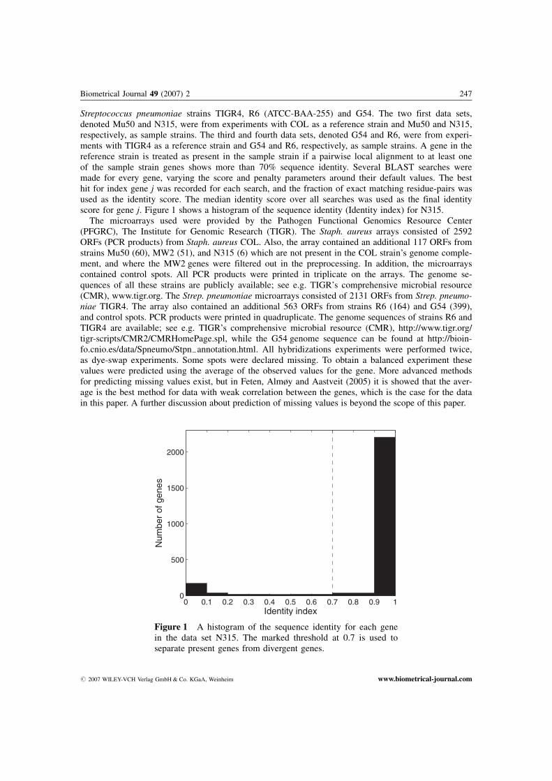
Streptococcus pneumoniae strains TIGR4, R6 (ATCC-BAA-255) and G54. The two first data sets,denoted Mu50 and N315, were from experiments with COL as a reference strain and Mu50 and N315,respectively, as sample strains. The third and fourth data sets, denoted G54 and R6, were from experi-ments with TIGR4 as a reference strain and G54 and R6, respectively, as sample strains. A gene in thereference strain is treated as present in the sample strain if a pairwise local alignment to at least oneof the sample strain genes shows more than 70% sequence identity. Several BLAST searches weremade for every gene, varying the score and penalty parameters around their default values. The besthit for index gene j was recorded for each search, and the fraction of exact matching residue-pairs wasused as the identity score. The median identity score over all searches was used as the final identityscore for gene j. Figure 1 shows a histogram of the sequence identity (Identity index) for N315.

The microarrays used were provided by the Pathogen Functional Genomics Resource Center(PFGRC), The Institute for Genomic Research (TIGR). The Staph. aureus arrays consisted of 2592ORFs (PCR products) from Staph. aureus COL. Also, the array contained an additional 117 ORFs fromstrains Mu50 (60), MW2 (51), and N315 (6) which are not present in the COL strain’s genome comple-ment, and where the MW2 genes were filtered out in the preprocessing. In addition, the microarrayscontained control spots. All PCR products were printed in triplicate on the arrays. The genome se-quences of all these strains are publicly available; see e.g. TIGR’s comprehensive microbial resource(CMR), www.tigr.org. The Strep. pneumoniae microarrays consisted of 2131 ORFs from Strep. pneumo-niae TIGR4. The array also contained an additional 563 ORFs from strains R6 (164) and G54 (399),and control spots. PCR products were printed in quadruplicate. The genome sequences of strains R6 andTIGR4 are available; see e.g. TIGR’s comprehensive microbial resource (CMR), http://www.tigr.org/tigr-scripts/CMR2/CMRHomePage.spl, while the G54 genome sequence can be found at http://bioin-fo.cnio.es/data/Spneumo/Stpn�annotation.html. All hybridizations experiments were performed twice,as dye-swap experiments. Some spots were declared missing. To obtain a balanced experiment thesevalues were predicted using the average of the observed values for the gene. More advanced methodsfor predicting missing values exist, but in Feten, Almøy and Aastveit (2005) it is showed that the aver-age is the best method for data with weak correlation between the genes, which is the case for the datain this paper. A further discussion about prediction of missing values is beyond the scope of this paper.


0 0.1 0.2 0.3 0.4 0.5 0.6 0.7 0.8 0.9 10

500

1000

1500

2000

Identity index

Num

ber

of g

enes

Figure 1 A histogram of the sequence identity for each genein the data set N315. The marked threshold at 0.7 is used toseparate present genes from divergent genes.


Hybridized arrays were scanned at wavelengths 532 nm (cyanine-3) and 635 nm (cyanine-5) at10 mm resolution to obtain two TIFF images, with a ScanArrayExpress Microarray Scanner (PackardBioscience). Fluorescent intensities and spot morphologies were analyzed using the QuantArray pro-gram ver. 3.0 (Packard BioScience), and spots were excluded based on slide or morphology abnormal-ities.

The data were normalized with a procedure similar to the self-normalization described by Yanget al. (technical report available at http://www.stat.berkeley.edu/users/terry/zarray/Html/normspie.html),but extended with a smoothing of the gene-wise dye-effects over average log-intensity.

Let M0jai be the observed ratio intensity for gene j for spot i on array a. A gene-wise effect of dyecan be estimated from the linear model

M0jai ¼ mj þ djIa þ ejai ;

where mj is the expected ratio intensity for gene j, dj is the gene-wise effect of dye, Ia is 1 or �1depending on the dye used for the reference strain on array a, and ejai is noise. An effect of dyedependent on the total intensity, dðAÞ, can thus be found by smoothing the data ð �AAj; ddjÞ e.g. by thelowess smoother (Cleveland, 1979), where �AAj is the total intensity for gene j and ddj is the estimatedeffect of dye for gene j. Finally, the normalized ratio intensities for each spot Mjai are obtained as

Mjai ¼ M0jai � dðAjaiÞIa :

Figure 2 shows the MA-plots with all replicates for each gene in the four data sets, while thecorresponding plots with averaged values of each gene are shown in Figure 3. The variance uncondi-tioned on genes appears to be larger in data from experiments with strains G54 and R6 compared to


(a) (b)

(c) (d)

Figure 2 MA-plot of all replicates in Mu50 (a), N315 (b), G54 (c), and R6 (d). The reddots represent divergent genes, and the black dots represent present genes.


data from experiments with the strains Mu50 and N315 for both the ratio intensities and the totalintensities. Notice that the total intensities were smaller for Mu50 and N315 than for the other strains.

3.2 Numerical summaries of data

As an attempt to better understand the results, we studied the amount of total variability (measured bythe sum of squares) explained by the groups, i.e. the variability between the groups divided by thetotal variability. This amount is an indication of the possibility to divide the genes into two groupsbased on the information in the ratio intensities and in the total intensities. The amount of unex-plained variability, i.e. the variability within the genes divided by the total variability, give us informa-tion about the variability within the genes, and hence whether the mixture models should be fitted onthe averaged values of each gene, or on all the replicates. The amount of explained and unexplainedvariability is given in Table 2. For Mu50 the groups hardly explain anything of the variability neitherin the ratio intensities nor in the total intensities, hence poor classification must be expected. In theother strains, with R6 as the superior, the groups explain more of the variability, and better classifica-tion can be expected. Especially for Mu50 and N315 improvement with Model 3 and Model 4 com-pared to Model 1 and Model 2 might be achieved due to large variability within the genes.

By fitting a two-stage nested design with genes nested under groups an F-value for the test ofgroup effect is obtained (Montgomery, 1997). Let L ¼ jWj=jTj, where W is the sum of squares andproducts matrix within groups and T is the total sum of squares and products matrix, thenF ¼ dfdð1�

ffiffiffiffiLpÞ=0:5 dfn

ffiffiffiffiLp

, where dfd and dfn is the degrees of freedom for the denominator andthe numerator respectively (Mardia, Kent, and Bibby, 1979). The F-value gives more accurate informa-tion about the effect of group than just the amount of variance explained. Larger F-values indicates


(a) (b)

(c) (d)

Figure 3 MA-plot of the average for each gene in Mu50 (a), N315 (b), G54 (c), and R6(d). The red dots represent divergent genes, and the black dots represent present genes.


that the groups are well separated. Table 3 show the F-values from univariate (Mij) and multivariate(½Mij;Aij�t) analysis of variance of the data. Due to different degrees of freedom all the F-valuescannot be compared directly, but the results confirm that there is a smaller effect of group in Mu50than in the other data sets.

The information above hopefully gives valuable contribution to a better understanding of when onemodel is in preference to another. However, in general the true group of the genes is unknown, henceadditional information is needed as a guidance in the choice of model. Table 4 shows the average ofthe variance within genes and the variance between the genes for each strain respectively. We noticethat Mu50 has large variances within the genes, especially for the ratio intensities, while the variancebetween the genes is small. This indicates that poor classification must be expected, but with possibleimprovement for the models that include all replicates. The opposite is the case for strain G54, whichhave small variances within the genes and large variance between the genes. Strain N315 has largevariances of the intensities within the genes, while R6 has large variance of the intensities between thegenes.

3.3 Results

To validate the models, we applied the geometric average (GA) given in (4). The analysis of variancemodel (5) is used to test for significant differences between the models, between the number of com-ponents and between the data sets. If nothing else is stated, the reported differences are assumed


Table 2 The two first columns show the amount of total varia-bility explained by the groups when studying the ratio intensities(first column) and both the ratio intensities and total intensities(second column). The third column and the fourth column showthe amount of unexplained variability when studying the ratiointensities and both the ratio intensities and total intensities re-spectively.

Group Within gene

Strain Mij ½Mij; Aij� Mij ½Mij; Aij�

Mu50 0.02 0.02 0.48 0.33N315 0.10 0.05 0.25 0.30G54 0.15 0.08 0.09 0.11R6 0.20 0.06 0.16 0.14

Table 3 Overview of the F-values with the corresponding de-grees of freedom (for the numerator and the denominator respec-tively) for the test of group effect. The first column is with Mij

as response in an analysis of variance model, while the secondcolumn is with ½Mij; Aij�t as response in a multivariate analysisof variance.

Strain Mij ½Mij; Aij�t

Mu50 451.39 (1, 12860) 915.11 (2, 12859)N315 4994.73 (1, 12860) 3224.19 (2, 12859)G54 25502.77 (1, 14889) 15405.45 (2, 14888)R6 18544.22 (1, 14889) 11679.85 (2, 14888)


significant at 0.05 level, where the p-values are adjusted by the Tukey method (Montgomery, 1997).The corresponding residual plot is shown in Figure 4(a). The interaction between model and numberof components and the interaction between number of components and data set were both found insig-nificant, hence these terms are removed from the model before the analysis. The results for the differ-ent models with different choices of number of components are shown in Figure 5. As expected, poorclassification of the genes in Mu50 was obtained. The results indicate that for all strains except G54the best choice of model is Model 4, namely the one that includes all replicates for both the ratiointensity and the total intensity. Note that the difference between the models is only significant forN315 and R6. In N315 including the replicates is an improvement independent of the number ofcomponents in the model, while for the other strains this is only the case for most of the components.

For Mu50 best classification is obtained with three and four components in the mixture model,while for the other strains the optimal classification is obtained with two components (see Figure 5).However, the difference between the results for various number of components is not significant.

Model 1 fitted on strain G54 maximizes GA with three components, which can be explained by thefact that the ratio intensities are distributed with two heavy tails. The other strains have a heavy tail tothe left, and hence a model with two components should be fitted to the data. Since N315 and R6, inopposite to Mu50 and G54, have a distinct divergent tail in the MA-plot; great improvement in theclassification is achieved by including the total intensities in the model.

The geometric average (GA) for the different models are shown in Figure 6. The results are aver-aged over number of components and indicate that the best choice of model is the most complex one,namely the one that includes all the replicates for both the ratio and the intensity. Even if there aresignificant interaction effects between models and data sets, Model 4 is preferred for all data sets. It


Table 4 Variance within and between the genes

for each strain, where �ss2xj¼ 1

pðn�1ÞPpj¼1

Pni¼1ðxij � �xxjÞ2

and s2�xxj¼ 1

p�1

Ppj¼1ð�xxj��xxÞ2.

Strain �ss2Mj

�ss2Aj

s2�MMj

s2�AAj

Mu50 0.089 0.12 0.08 0.26N315 0.061 0.24 0.15 0.42G54 0.033 0.09 0.30 0.54R6 0.064 0.13 0.25 0.62

(a) (b)

Figure 4 Plot of residuals versus fitted values for Model (5) with GA (a) and AUC (b)as response.


can be shown that the models with two and three components achieved better assignments to thegroups than the models with five components. The genes in Mu50 are as assumed hardest to assign tothe correct group.


(a) (b)

(c) (d)

Figure 5 Plot of GA for different models and number of components for Mu50 (a),N315 (b), G54 (c), and R6 (d). Model 1 (—*—), Model 2 (---^---), Model 3 (– –&– –),and Model 4 (–-–~–-–).

Figure 6 Plot of GA for different models for Mu50 (– –&– –),N315 (---^---), R6 (–-–~–-–), and G54 (—*—).


The optimal model for each strain was found with the classification limit 0.5. Validation of themodels with other choices of classification limits is also interesting; in this study this is done byROC-curves. Model (5) with AUC as response is used to test for significant differences. The re-ported differences are, if nothing else is stated, assumed significant at 0.05 level, where the p-valuesare adjusted by the Tukey method. The corresponding residual plot is shown in Figure 4(b). Theinteraction between number of components and data set was found insignificant, hence this term isremoved from the model before the analysis. The results from every combination of model andnumber of components will not be presented, only the ones that are best based on GA and AUCrespectively. Figure 7 shows the ROC-curves for the best choice of both model and components forthe different strains. For strain Mu50, Model 4 with four components achieved the largest, but insig-nificantly, improvement compared to the model with highest GA, where AUC increases from 0.58 to0.76, in addition GA is almost unchanged (decreases from 0.50 to 0.48). This is the strain withlargest overlapping region between the two groups, and hence poorest possibility to assign the genesinto correct group. For the other strains the improvement is not that large, and in addition GAbecomes a lot smaller, especially for N315 and R6. For strain G54 AUC increases from 0.76 to 0.82by Model 2 with four components, while GA decreases from 0.69 to 0.63, but none of the changesare significant. For strain N315 and R6 an improvement in AUC from 0.86 to 0.91 and from 0.75 to0.83 is obtained, respectively, both by Model 2 with five components, while GA decreases from0.78 to 0.66 and from 0.71 to 0.57. However, there is no significant difference between Model 2and Model 4.


(a) (b)

(c) (d)

Figure 7 ROC curves for the optimal model based on GA (lower curve, black) and forthe optimal model based on AUC (upper curve, grey) for Mu50 (a), N315 (b), G54 (c),and R6 (d). The fraction of truly divergent genes is on the vertical axis, and the fractionof falsely divergent genes is on the horizontal axis.


The area under curve seems to be almost unaffected by the number of components for the modelsbased on the ratio intensities (results not shown). For the model based on the average of the ratiointensities and the average of the total intensities (Model 2) AUC is increasing with increasing num-ber of components, except for strain Mu50. Most of the genes in the overlapping region in Figure 3are present. When a mixture model with three components is fitted, most of these genes will beassigned to the present group with larger probability than when a mixture model with two componentsis fitted. Since most of these genes are truly present, AUC will increase. Notice that the differencebetween AUC for different number of components is not significant.

In Table 5 the results obtained with mixture models, maximizing GA and AUC respectively, arecompared with the corresponding results from the GACK approach by Kim et al. (2002). For two outof four classification with mixture models based on GA gives better results than GACK, while forthree out of four classification with mixture models based on AUC gives better results than GACK.One explanation might be that GACK has its benefits when the distribution of the group of presentgenes is symmetric, while mixture models solve deviation from a symmetrical distribution by addingmore components to the model. Notice that the difference between the method is small when GACKachieves better results, while it is larger when mixture models achieve better results.

4 Discussion

The aim of this paper was to study four different mixture models’, each with four different number ofcomponents, capability to assign genes into groups of divergent and present. Different numerical sum-maries of the data were given as a guide in the choice of model and number of components, whiletwo criteria together with analysis of variance were used to validate the models.

In this paper we have used two criteria in the validation of the methods. The first criterion, denotedGA, measures the geometric average of the estimated probability of correct classification of a diver-gent gene and the estimated probability of correct classification of a present gene given a classifica-tion limit. The second criterion, denoted AUC, measures the models’ ability to divide the genes fordifferent limits. Since the interest is in the classification error received for a given limit, the modelswere mainly validated by GA. A more thorough comparison of the validation criteria are important,but beyond the scope of this paper.

The mixture models in this paper assume a normal distribution of the log2-intensity ratios (ratiointensities) and the average log2-intensities (total intensities), and hence of the log2 intensities them-selves. Different tests for normality rejected the hypothesis that the log2-intensities of the data in ourstudy follow a normal distribution. However, the method based on mixture models seems to be robustagainst small deviations from this assumption.


Table 5 The table gives an overview of GA and AUC obtained by mixture modelsand by GACK. In the columns of Mixture1 the results from the mixture modelsmaximizing GA are shown, while in the columns of Mixture2 the results from themixture models maximizing AUC are shown. The results from GACK are obtainedwith the estimated probability of presence cutoff equal to 0.5.

GA AUC

Strain Mixture1 Mixture2 GACK Mixture1 Mixture2 GACK

Mu50 0.50 0.48 0.55 0.58 0.76 0.62N315 0.78 0.66 0.50 0.86 0.91 0.73G54 0.69 0.63 0.50 0.76 0.82 0.79R6 0.71 0.57 0.75 0.75 0.83 0.84


It is common to assume that the genome of the reference strain consists of regions each of which isdominantly present or dominantly divergent in the sample strain (Wang and Guo, 2004). This spatialinformation was used to smooth the estimated posterior probabilities by moving average. However, thegenes’ position on the genome did not improve the classification, hence the results were not includedin the paper.

The structure of the covariance matrices does not consider that the experiment is a dye swap experi-ment, i.e. the replicates are from two arrays. Since the complexity of the models increase when includ-ing array effect and the effect of array is supposed to be removed in the normalization, we found thisrefinement not necessary.

If the interest is to find the minimal genome common to both the reference and the sample strain, itmay be an advantage to increase the classification limit above 0.5. Then the fraction of truly presentgenes is increasing, and the predicted minimal genome is correct with larger probability.

In the data sets analyzed in our study mixture models improved the classification of present anddivergent genes compared to the previously published method GACK in some cases, but not in all.Mixture models seems to be in preference for data sets where the main peak is non-symmetric aroundits maximum and for data sets with two apparent regions in the MA-plot.

The results indicated that large variance between the genes give good classification. This is notnecessarily universal, since the groups still might be overlapping. However, data sets with two relativeclear regions in the MA-plot seemed to give good classification independent of model and componentchoice. Each of the two regions consists of divergent and present genes, while the overlapping regionconsists of both, but most present genes since they are in majority on the genome.

If the mixture models are fitted with the replicates of the genes and not the average within eachgene, the increase in number of parameters is small compared to the total number of observations, andthe classification is in general improved, even for data with small variances within the genes. Whenthe amount of variance explained by the group is extremely small, the improvement in classification isnegligible.

This study showed that best classification is obtained by fitting mixture models with both ratiointensities and total intensities for all replicates of the genes. Based on the geometric average of theestimated probability of correct assignment of divergent genes and present genes (GA) the modelsshould be fitted with two components, but by increasing the number of components the area under theROC-curve is increased without too much loss in GA.

Acknowledgements We thank the Pathogen Functional Genomics Resource Center (PFGRC), The Institute forGenomic Research (TIGR), Rockville, MD for providing microarrays. The Staph. aureus Mu50 were kindly pro-vided by Lisa Herron, University of Minnesota, St. Paul, MN, while prof. Hans-Georg Sahl, University of Bonn,Germany provided us with the Staph. aureus COL and N315 strains. The Strep. pneumoniae G54 strain wasprovided to us by Dr. Francesco Iannelli, University of Siena, Italy, while Dr. Ingeborg S. Aaberge, The Norwe-gian Institute of Public Health, offered the Strep. pneumoniae TIGR4 strain to us.

We would like to thank two anonymous referees for constructive criticism. The Norwegian University of LifeSciences has financed this work.

Appendix-Maximum likelihood estimators

For cases were there is no constraints neither on the expectation vectors nor on the covariance ma-trices, the maximum likelihood estimators (MLEs) of the unknown parameters in the ðqþ 1Þ-th itera-tion are given by

mmðqþ1Þc ¼

Ppj¼1

zzðqÞj;c xj

Ppj¼1

zzðqÞj;c

; ð6Þ



and

SSðqþ1Þc ¼

Ppj¼1

zzðqÞj;c ðxj � mmðqþ1Þc Þðxj � mmðqþ1Þ

c Þt

Pnj¼1

zzðqÞj;c

; ð7Þ

respectively (McLachlan and Peel, 2000). For simplicity the iteration number is omitted in the follow-ing.

For the univariate model (Model 1) and the bivariate model (Model 2) the MLEs in the log like-lihood function in (2) are given in Equation (6) and Equation (7).

For the models with constraints either in the expectation vectors or in the covariance matrices, or inboth, the MLEs can be found in most books in advanced multivariate analysis, e.g. Mardia et al.(1979). In Model 3 the MLE of mM;c is given by

mmM;c ¼Pni¼1

mmðiÞ;c =n ;

where mmðiÞ;c is element i in mmc from (6), while the MLE of the variance of Mij and the correlationbetween Mij and Mi0j is given by

ss2M;c ¼

Pni¼1

SSðiiÞ;c =n ;

and

qqM;c ¼ 2Pi<i0

SSðii0Þ;c =½nðn� 1Þ ss2M;c� ;

respectively, where SSðii0Þ; c is element ði; i0Þ in SSc as given in (7).With the constraints in Model 4 the MLE of the expectations are given by

mmM;c ¼Pni¼1

mmðiÞ; c=n ;

and

mmA;c ¼P2n

i¼nþ1mmðiÞ;c=n :

The MLE of the variances are given by

ss2M;c ¼

Pni¼1

SSðiiÞ;c=n ;

and

ss2A;c ¼

P2n

i¼nþ1SSðiiÞ;c=n ;

while the corresponding correlations are estimated by

qqM;c ¼ 2P

i<i0�nSSðii0Þ;c =½nðn� 1Þ ss2

M;c� ;

and

qqA;c ¼ 2P

nþ1<i<i0SSðii0Þ;c =½nðn� 1Þ ss2

A;c� :



The MLE of the covariance between Mij and Ai0j for i ¼ i0 is given by

ssðMAÞS;c ¼Pni¼1

SSðnþiÞ;i;c=n ;

while for i 6¼ i0

ssðMAÞD;c ¼ 2P

i<i0�nSSðnþi;i0Þ;c=½nðn� 1Þ� :

References

Autio, R., Hautaniemi, S., Kauraniemi, P., Yli-Harja, O., Astola, J., Wolf, M., and Kallioniemi, A. (2003). CGH-plotter: MATLAB toolbox for CGH-data analysis. Bioinformatics 19, 1714–1715.

Behr, M. A., Wilson, M. A., Gill, W. P., Salamon, H., Schoolnik, G. K., Rane, S., and Small, P. M. (1999).Comparative genomics of BCG vaccines by whole-genome DNA microarray. Science 284, 1520–1532.

Bj�rkholm, B., Lundin, A., Sillen, A., Guillemin, K., Salama, N., Rubio, C., Gordon, J. I., Falk, P., and Eng-strand, L. (2001). Comparison of genetic divergence and fitness between two subclones of Helicobacterpylori. Infection and Immunity 69, 7832–7838.

Carothers, A. D. (1997). A likelihood-based approach to the estimation of relative DNA copy number by com-parative genomic hybridization. Bioinformatics 53, 848–856.

Cleveland, W. S. (1979). Robust locally weighted regression and smoothing scatterplots. Journal of the AmericanStatistical Association 74, 829–836.

Dempster, A. P, Laird, N. M., and Rubin, D. B. (1977). Maximum likelihood from incomplete data via the EMalgorithm (with Discussion). Journal of the Royal Statistical Society Series B –– Statistical Methodology 39,1–38.

Dziejman, M., Balon, E., Boyd, D., Fraser, C. M., Heidelberg, J. F., and Mekalanos, J. J. (2002). Comparativegenomic analysis of Vibrio cholerae: genes that correlate with cholera endemic and pandemic disease. Pro-ceedings of the National Academy of Sciences of the United States of America 99, 1556–1561.

Feten, G., Almøy, T., and Aastveit, A.H. (2005). Prediction of missing values in microarray and use of mixedmodels to evaluate the predictors. Statistical Applications in Genetics and Molecular Biology 4, No. 1, Arti-cle 10. http://www.bepress.com/sagmb/vol4/iss1/art10.

Feten, G., Almøy, T., Snipen, L., Aakra, �., and Aastveit, A. H. (2006). Regression as a method to predict copynumbers in comparative genomic hybridization studies on bacteria. Biometrical Journal 48, 255–270.

Fridlyand, J., Snijders, A., Pinkel, D., Albertson, D., and Jain, A. (2003). Statistical issues in the analysis of thearray CGH data. Proceedings of the Computational Systems Bioinformatics, 407–408.

Indahl, U. G., and Næs, T. (1998). Evaluation of alternative spectral feature extraction methods of textural imagesfor multivariate modeling. Journal of Chemometrics 12, 261–278.

Irizarry, R. A., Ooi, S. L., Wu, Z., and Boeke, J. D. (2003). Use of mixture models in a microarray-based screen-ing procedure for detecting differentially represented yeast mutants. Statistical Applications in Genetics andMolecular Biology 2, No. 1, Article 1. http://www.bepress.com/sagmb/vol2/iss1/art1.

Kim, C. C., Joyce, E. A., Chan, K., and Falkow, S. (2002). Improved analytical methods for microarray-basedgenome-composition analysis. Genome Biology 3, research 0065.1–0065.17.

Kubat, M., Holte, R., and Matwin, S. (1998). Machine learning for the detection of oil spills in satellite radarimages. Machine Learning 30, 195–215.

Lee, M.-L. T., Kuo, F. C., Whitmore, G. A., and Sklar, J. (2000). Importance of replication in microarray geneexpression studies: Statistical methods and evidence from repetetive cDNA hybridizations. Proceedings of theNational Academy of Sciences of the United States of America 97, 9834–9839.

Lewin, B. (2000). Genes VII. Oxford University Press Inc., New York.Lindman, H. R. (1992). Analysis of Variance in Experimental Design. Springer-Verlag, New York.McLachlan, G. J., Do, K.-A., and Ambroise, C. (2004). Analyzing Microarray Gene Expression Data. John Wiley

& Sons.McLachlan, G. J. and Peel, D. (2000). Finite Mixture Models. John Wiley & Sons.Mardia, K. V., Kent, J. T., and Bibby, J. M. (1979). Multivariate Analysis. Academic Press, London.Montgomery, D. C. (1997). Design and analysis of experiments. John Wiley & Sons.



Moore, D. H., Pallavicini, M., Cher, M. L., and Gray, J. W. (1997). A t-statistic for objective interpretation ofcomparative genomic hybridization (CGH) profiles. Cytometry 28, 183–190.

Murray, A. E., Lies, D., Li, G., Nealson, K., Zhou, J., and Tiedje, J. M. (2001). DNA/DNA hybridization tomicroarrays reveals gene-specific differences between closely related microbial genomes. Proceedings of theNational Academy of Sciences of the United States of America 98, 9853–9858.

Nguyen, D. V., Arpat, A. B., Wang, N. Y., and Carroll, R. J. (2002). DNA Microarray Experiments: Biologicaland Technological Aspects. Biometrics 58, 701–717.

Peng, D. F., Sugihara, H., Sho, K., Mukaisho, K., Tsubosa, Y., and Hattori, T. (2003). Alterations of chromosomalcopy number during progression of diffuse-type gastric carcinomas: metaphase- and array-based comparativegenomic hybridization analyses of multiple samples from individual tumours. Journal of Pathology 201,439–450.

Pollack, J. R., Perou, C. M., Alizadeh, A. A., Eisen, M. B., Pergamenschikov, A., Williams, C. F., Jeffrey, S. S.,Botstein, D., and Brown, P. O. (1999). Genome-wide analysis of DNA copy-number changes using cDNAmicroarrays. Nature Genetics 23, 41–46.

Pollack, J. R., Sorlie, T., Perou, C. M., Rees, C. A., Jeffrey, S. S., Lonning, P. E., Tibshirani, R., Botstein, D.,Borresen-Dale, A. L., and Brown, P. O. (2002). Microarray analysis reveals a major direct role of DNA copynumber alteration in the transcriptional program of human breast tumors. Proceedings of the National Acad-emy of Sciences of the United States of America 99, 12963–12968.

Repsilber, D., Mira, A., Lindroos, H., Andersson, S., and Ziegler, A. (2005). Data rotation improves genomotyp-ing efficiency. Biometrical Journal 47, 585–598.

Salama, N., Guillemin, K., McDaniel, T. K., Sherlock, G., Tompkins, L., and Falkow, S. (2000). A whole-genomemicroarray reveals genetic diversity among Helicobacter pylori strains. Proceedings of the National Academyof Sciences of the United States of America 97, 14668–14673.

Swets, J. A. (1988). Measuring the accuracy of diagnostic systems. Science 240, 1285–1293.Veltman, J. A., Fridlyand, J., Pejavar, S., Olshen, A. B., Korkola, J. E., DeVries, S., Carroll, P., Kuo, W. L.,

Pinkel, D., Albertson, D., Cordon-Cardo, C., Jain, A. N., and Waldman, F. M. (2003). Array-based compara-tive genomic hybridization for genome-wide screening of DNA copy number in bladder tumors. CancerResearch 63, 2872–2880.

Wang, Y. D. and Guo, S. W. (2004). Statistical methods for detecting genomic alterations through array-basedcomparative genomic hybridization (CGH). Frontiers in Bioscience 9, 540–549.



Mixture Models as a Method to Find Present and Divergent Genes in Comparative Genomic Hybridization...

Documents

Transcript of Mixture Models as a Method to Find Present and Divergent Genes in Comparative Genomic Hybridization...