DISCUSSION PAPER SERIES

IZA DP No. 13987

Alexander AhammerStefan BauernschusterMartin HallaHannah Lachenmaier

Minimum Legal Drinking Age and the Social Gradient in Binge Drinking

DECEMBER 2020

Any opinions expressed in this paper are those of the author(s) and not those of IZA. Research published in this series may include views on policy, but IZA takes no institutional policy positions. The IZA research network is committed to the IZA Guiding Principles of Research Integrity.The IZA Institute of Labor Economics is an independent economic research institute that conducts research in labor economics and offers evidence-based policy advice on labor market issues. Supported by the Deutsche Post Foundation, IZA runs the world’s largest network of economists, whose research aims to provide answers to the global labor market challenges of our time. Our key objective is to build bridges between academic research, policymakers and society.IZA Discussion Papers often represent preliminary work and are circulated to encourage discussion. Citation of such a paper should account for its provisional character. A revised version may be available directly from the author.

Schaumburg-Lippe-Straße 5–953113 Bonn, Germany

Phone: +49-228-3894-0Email: publications@iza.org www.iza.org

IZA – Institute of Labor Economics

DISCUSSION PAPER SERIES

ISSN: 2365-9793

IZA DP No. 13987

Minimum Legal Drinking Age and the Social Gradient in Binge Drinking

DECEMBER 2020

Alexander AhammerJKU and CDECON

Stefan BauernschusterUniversity of Passau, IZA and CESifo

Martin HallaJKU, CDECON, IZA and GÖG

Hannah LachenmaierUniversity of Passau

ABSTRACT

IZA DP No. 13987 DECEMBER 2020

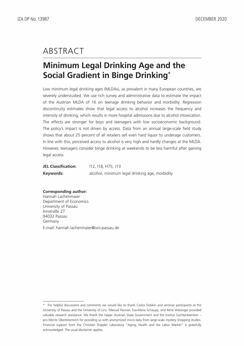
Minimum Legal Drinking Age and the Social Gradient in Binge Drinking*

Low minimum legal drinking ages (MLDAs), as prevalent in many European countries, are

severely understudied. We use rich survey and administrative data to estimate the impact

of the Austrian MLDA of 16 on teenage drinking behavior and morbidity. Regression

discontinuity estimates show that legal access to alcohol increases the frequency and

intensity of drinking, which results in more hospital admissions due to alcohol intoxication.

The effects are stronger for boys and teenagers with low socioeconomic background.

The policy’s impact is not driven by access. Data from an annual large-scale field study

shows that about 25 percent of all retailers sell even hard liquor to underage customers.

In line with this, perceived access to alcohol is very high and hardly changes at the MLDA.

However, teenagers consider binge drinking at weekends to be less harmful after gaining

legal access.

JEL Classification: I12, I18, H75, J13

Keywords: alcohol, minimum legal drinking age, morbidity

Corresponding author:Hannah LachenmaierDepartment of EconomicsUniversity of PassauInnstraße 2794032 PassauGermany

E-mail: hannah.lachenmaier@uni-passau.de

* For helpful discussions and comments we would like to thank Carlos Dobkin and seminar participants at the

University of Passau and the University of Linz. Manuel Pannier, Eva-Maria Schaupp, and Rene Wiesinger provided

valuable research assistance. We thank the Upper Austrian State Government and the Institut Suchtprävention –

pro Mente Oberösterreich for providing us with anonymized micro data from large-scale mystery shopping studies.

Financial support from the Christian Doppler Laboratory “Aging, Health and the Labor Market” is gratefully

acknowledged. The usual disclaimer applies.

I. Introduction

Europe has the highest level of alcohol consumption in the world. In 2016, more than 10.3 mil-lion disability-adjusted life-years were lost due to alcohol abuse in the EU+ (European Unionmember states, Norway and Switzerland) (World Health Organization, 2019). More than 10percent of all deaths in Europe are attributable to alcohol abuse (World Health Organization,2018). The comparatively low minimum legal drinking ages (MLDA) in Europe are often con-sidered as one explanation for the higher prevalence of teenage binge drinking relative to theUS. While most of the European countries uphold an MLDA of 18 years, some countries, suchas Austria, Belgium, Denmark, Germany, or Switzerland, allow on- and off-premise sales ofbeer and wine to teenagers as young as 16 years. Critics of a low MLDA argue that an early on-set of drinking can have detrimental long-run effects on both physical and mental health, sincethe developing brain is particularly vulnerable to the impact of alcohol (Ewing et al., 2014). Incontrast, proponents argue that allowing teenagers the experience of drinking at an earlier ageresults in more responsible alcohol consumption.

Over the last decade, we have witnessed rising interest in the impact of MLDA regulation onrisky behavior and health. Many studies use survey data to investigate the impact of the MLDAon alcohol and drug consumption (Carpenter et al., 2007; Crost and Guerrero, 2012; Yörükand Yörük, 2011; Crost and Rees, 2013; Deza, 2015). Studies that use administrative datatypically focus on the impact of the MLDA on mortality, in particular fatal accidents (Dee, 1999;Carpenter and Dobkin, 2009; Carpenter et al., 2016), but also crime (Carpenter and Dobkin,2015; Hansen and Waddell, 2018; Chalfin et al., 2019) or schooling (Carrell et al., 2011; Lindoet al., 2013). Due to data constraints, only few studies were able to investigate morbidity effectsof the MLDA, although these effects constitute a major cost factor in health systems (Carpenterand Dobkin, 2017; Callaghan et al., 2013). Moreover, the existing evidence on the effectsof MLDA regulation stems almost exclusively from the U.S. or Canada, where the MLDAis considerably higher than in Europe.1 Finally, even though MLDA regulation might havevarying impacts across the socioeconomic distribution, little is known about these potentiallyheterogeneous effects. This is not least due to a lack of access to administrative data on teenagehealth outcomes that can be linked to data on parental characteristics.

We apply a regression discontinuity (RD) design to comprehensively study the impact ofa particularly low MLDA of 16 years in Austria, a country with very high alcohol consump-tion by international comparison. We start with rich survey data from the European School

Survey Project on Alcohol and Other Drugs (ESPAD) to understand the impact of the MLDAon teenagers’ self-reported drinking behavior. The detailed information provided in the survey

1The notable exceptions analyze the impact of a decrease in the MLDA from 20 to 18 in New Zealand (Boesand Stillman, 2013, 2017; Conover and Scrimgeour, 2013) and the impact of an MLDA of 18 in Australia (Lindoet al., 2016) on hospitalizations and mortality. Only recently, the first papers appeared that investigate MLDAeffects in European countries with a low MLDA of 16 (Datta-Gupta and Nilsson, 2020; Dehos, 2020; Kamalowand Siedler, 2019).

2

data allows us to go beyond average effects, and estimate MLDA effects along the drinkingdistribution. In a next step, we use administrative data from a universal healthcare providerto investigate the effects of the MLDA on alcohol-related hospitalizations. In all analyses, westudy heterogeneous effects by socioeconomic background and gender. In a final step, we pro-vide evidence on the mechanisms underlying these effects. In particular, we ask to which degreethe MLDA restricts access to alcohol. To this end, we obtained data from an annual large-scalefield study, which sends underage test buyers to retailers in an attempt to buy alcohol. Addition-ally, we examine information provided in the ESPAD on teenagers’ perceived access to alcoholas well as attitudes towards alcohol.

Our results show that upon gaining legal access to alcohol, teenagers significantly increasethe frequency and intensity of drinking, which results in negative health effects. The probabilityof drinking alcohol on at least one day during the last week increases by around 12 percentagepoints, the probability of drinking at least two days increases by 9 percentage points, and theprobability of drinking on at least three days increases by 4 percentage points. In terms ofquantities, we find that the probability of consuming at least 180 to 240 grams of pure alcohol(which corresponds to an extra nine to twelve pints of beer) during the last week increasesby 10 percentage points. The MLDA effects are larger for boys and for teenagers with lowsocioeconomic background. This change in drinking behavior results in negative health effects.We find that the probability of being hospitalized with an alcohol intoxication increases by0.036 percentage points or 42 percent at the MLDA cutoff. Again, these effects are larger forboys and for teenagers with low socioeconomic background. Interestingly, these socioeconomicgradients are not visible prior to gaining legal access to alcohol. Instead, they emerge at theMLDA cutoff, become statistically significant and economically meaningful, and then remainvisible until the age of 22. These results are robust to using different functional forms andkernel weighting techniques. Teenagers from families with a history of severe alcohol abuse area notable exception. For this high risk group, MLDA is not effective at all.

Investigating the mechanisms behind these effects, we show that MLDA legislation does notseverely impede teenagers’ access to alcohol. The mystery shopping data indicate that about25 percent of all retailers sell even hard liquor to underage customers. When asking teenagershow difficult it is to get access to alcohol, the MLDA legislation seems to be even less binding:Roughly 85 percent of teenagers below 16 years of age perceive access to non-distilled alcoholas easy. This set of results suggests that the negative impact of MDLA legislation on alco-hol consumption can hardly be fully explained by restrictions to alcohol access. Interestingly,the share of teenagers who perceive regular heavy drinking at weekends as risky significantlydeclines from 70 to 60 percent at the MLDA cutoff too. We argue that this might reflect a nor-mative impact of the legislation. Teenagers below 16 years of age may simply feel obliged toobey and abstain from drinking despite its availability. Once drinking becomes legally allowedand also socially more accepted, teenagers change their attitudes towards alcohol and drinkmore frequently and more intensely. Our findings do not support the idea that lower MLDAs

3

help teenagers to ease into drinking and to consume alcohol responsibly (Wechsler and Nelson,2006).

Most closely related to our work is a paper by Datta-Gupta and Nilsson (2020). They showthat the introduction of a MLDA of 15 in Denmark and the following increases to 16 and 18 (forhard liquor) reduced injuries but had no significant impact on alcohol intoxication. The authorsfind different responses for boys and girls, but no consistent differences across socioeconomicgroups. An important difference between Datta-Gupta and Nilsson (2020) and our setting isthat alcohol is very cheap in Austria, in particular in comparison to Denmark and the otherScandinavian countries, which should be particularly relevant for the consumption decision ofteenagers whose budget is limited. Moreover, Datta-Gupta and Nilsson (2020) use a difference-in-differences setup to estimate the impact of changes in the MLDA. The treatment group isunder 15 year olds for their first reform (i.e., the introduction of a MLDA), 15–16 year olds fortheir second reform (i.e., the increase of the MLDA), and 16–18 year olds for their third reform(i.e., the increase of the MLDA for hard liquor). In contrast, we apply an RD design to estimatethe impact of gaining access to alcohol for teenagers after they turned 16. Thus, we exploit adifferent margin of the MLDA treatment. Finally, while Datta-Gupta and Nilsson (2020) userich administrative data, we combine administrative data with survey data and data from a fieldstudy to also investigate the channels behind the effects.

The remainder of the paper is structured as follows. Section II provides background infor-mation on alcohol consumption and MLDA laws in Austria. Section III introduces the surveyand administrative data used, while Section IV presents the RD design that we apply to estimatethe causal effects of the MLDA on drinking and health. In Section V, we present the empiricalresults. In Section VI, we compare adolescent drinking behavior in Austria and the U.S. Thishelps to relate our results to the existing US-dominated literature. Section VII concludes thepaper.

II. Background

II.1. Alcohol consumption in Austria

Over the past 60 years, alcohol consumption has markedly converged across countries. Theleft panel of Figure 1 plots per capita consumption of pure alcohol in liters for several Westernindustrialized countries from 1960 to 2014.2 While France and Italy started at very high levels,they have substantially reduced alcohol consumption between 1960 and 2014. Great Britainand the U.S. on the other hand started at lower levels, but have seen increasing consumptionover this period.

To better understand the intensity of drinking among people who generally drink alcohol, it

2The per capita consumption variable does not exclude children. Consequently, average alcohol consumptionlevels of adults are clearly higher than depicted here. The data have been collected by Holmes and Anderson(2017).

4

is worthwhile to investigate patterns of binge drinking. A common measure used to this end isthe share of drinkers (15 years and older), who have had at least 60 grams of pure alcohol onat least one occasion during the past 30 days. Note that 60 grams of alcohol correspond to sixstandard drinks or to roughly half a litre of wine or three pints of beer, respectively. The rightpanel of Figure 1 shows that the share of people having had a binge drinking incidence duringthe past month varies substantially across countries.3 While binge drinking is rather uncommonin New Zealand or Italy, around a quarter of adults in the U.S. experienced at least one heavydrinking incidence during the past month. In Great Britain, even every third person who drinksalcohol had at least one binge drinking incidence during the past month.

Figure 1 shows that Austria stands out in both average alcohol consumption and the occur-rence of binge drinking among regular drinkers. In the left panel, we observe that Austria’sper capita consumption of pure alcohol was already at a rather high level of 8.7 liters in 1960and even further increased over the following decades. With a per capita consumption of 10.4liters in 2014, Austria has a higher alcohol consumption level than any other country depictedin this figure. In the right panel, we see that more than 50 percent of all drinkers aged 15 andolder in Austria had at least one binge drinking incidence during the past month. This numberis considerably higher than in any other country listed in this figure. These facts make Austriaa particularly interesting country to study the impact of a low MLDA on alcohol abuse.

II.2. Austria’s MLDA laws

In Austria, legal access to alcohol is regulated by MLDA laws as part of the Law for the Protec-tion of Children and Young People.4 Before the laws were harmonized in 2019, MLDA variedacross the Austrian federal states. Most states permitted teenagers to legally access non-distilledalcohol such as beer and wine at the age of 16, and distilled alcohol at the age of 18.5 The statesof Burgenland, Lower Austria, and Vienna allowed universal legal access to both non-distilledand distilled alcohol at the age of 16. As part of the harmonization process in 2019, the agelimits were set to 16 for non-distilled alcohol and 18 for distilled alcohol country-wide.

The state-specific laws also define sanctions in case of non-compliance. The severity ofthese sanctions vary depending on whether minors, adults, or companies violate the laws.6 Non-compliance of teenagers is defined as acquiring or consuming alcoholic beverages below theMLDA threshold, or providing other teenagers below this threshold with alcoholic beverages.In case of violation of the law, authorities may require teenagers to participate in an instructionand consultation meeting or to do community service. Moreover, monetary fines for repeated

3The data from 2010 are published by World Health Organization Global Health Observatory (GHO).4Besides the minimum legal drinking age, the law also defines minimum legal ages to acquire tobacco and

related products and permitted hours for adolescents of different age.5This gradual access to alcohol depending on its alcohol content can also be found in other European coun-

tries such as Belgium, Denmark, Germany, or Sweden (see https://fra.europa.eu/en/publication/2017/mapping-minimum-age-requirements/purchase-consumption-alcohol).

6See https://www.oesterreich.gv.at/themen/jugendliche/jugendrechte/6.html

5

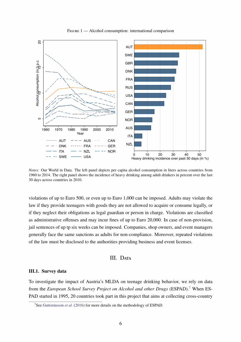
Figure 1 — Alcohol consumption: international comparison

510

1520

Alco

hol c

onsu

mpt

ion

(in l)

p.c

.

1960 1970 1980 1990 2000 2010Year

AUT AUS CANDNK FRA GERITA NZL NORSWE USA 0 10 20 30 40 50

Heavy drinking incidence over past 30 days (in %)

NZL

ITA

AUS

NOR

GER

CAN

USA

RUS

FRA

DNK

GBR

SWE

AUT

Notes: Our World in Data. The left panel depicts per capita alcohol consumption in liters across countries from1960 to 2014. The right panel shows the incidence of heavy drinking among adult drinkers in percent over the last30 days across countries in 2010.

violations of up to Euro 500, or even up to Euro 1,000 can be imposed. Adults may violate thelaw if they provide teenagers with goods they are not allowed to acquire or consume legally, orif they neglect their obligations as legal guardian or person in charge. Violations are classifiedas administrative offenses and may incur fines of up to Euro 20,000. In case of non-provision,jail sentences of up tp six weeks can be imposed. Companies, shop owners, and event managersgenerally face the same sanctions as adults for non-compliance. Moreover, repeated violationsof the law must be disclosed to the authorities providing business and event licenses.

III. Data

III.1. Survey data

To investigate the impact of Austria’s MLDA on teenage drinking behavior, we rely on datafrom the European School Survey Project on Alcohol and other Drugs (ESPAD).7 When ES-PAD started in 1995, 20 countries took part in this project that aims at collecting cross-country

7See Guttormsson et al. (2016) for more details on the methodology of ESPAD.

6

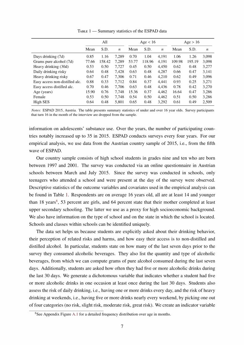
Table 1 — Summary statistics of the ESPAD data

All Age < 16 Age > 16

Mean S.D. n Mean S.D. n Mean S.D. n

Days drinking (7d) 0.85 1.16 7,289 0.70 1.04 4,191 1.06 1.26 3,098Grams pure alcohol (7d) 77.66 158.42 7,289 53.77 118.96 4,191 109.98 195.19 3,098Heavy drinking (30d) 0.53 0.50 7,727 0.45 0.50 4,450 0.62 0.48 3,277Daily drinking risky 0.64 0.48 7,428 0.63 0.48 4,287 0.66 0.47 3,141Heavy drinking risky 0.67 0.47 7,306 0.71 0.46 4,210 0.62 0.49 3,096Easy access non-distilled alc. 0.88 0.33 7,712 0.84 0.37 4,441 0.93 0.25 3,271Easy access distilled alc. 0.70 0.46 7,706 0.63 0.48 4,436 0.78 0.42 3,270Age (years) 15.90 0.76 7,748 15.36 0.37 4,462 16.64 0.47 3,286Female 0.53 0.50 7,748 0.54 0.50 4,462 0.51 0.50 3,286High SES 0.64 0.48 5,801 0.65 0.48 3,292 0.61 0.49 2,509

Notes: ESPAD 2015, Austria. The table presents summary statistics of under and over 16 year olds. Survey participantsthat turn 16 in the month of the interview are dropped from the sample.

information on adolescents’ substance use. Over the years, the number of participating coun-tries notably increased up to 35 in 2015. ESPAD conducts surveys every four years. For ourempirical analysis, we use data from the Austrian country sample of 2015, i.e., from the fifthwave of ESPAD.

Our country sample consists of high school students in grades nine and ten who are bornbetween 1997 and 2001. The survey was conducted via an online questionnaire in Austrianschools between March and July 2015. Since the survey was conducted in schools, onlyteenagers who attended a school and were present at the day of the survey were observed.Descriptive statistics of the outcome variables and covariates used in the empirical analysis canbe found in Table 1. Respondents are on average 16 years old, all are at least 14 and youngerthan 18 years8, 53 percent are girls, and 64 percent state that their mother completed at leastupper secondary schooling. The latter we use as a proxy for high socioeconomic background.We also have information on the type of school and on the state in which the school is located.Schools and classes within schools can be identified uniquely.

The data set helps us because students are explicitly asked about their drinking behavior,their perception of related risks and harms, and how easy their access is to non-distilled anddistilled alcohol. In particular, students state on how many of the last seven days prior to thesurvey they consumed alcoholic beverages. They also list the quantity and type of alcoholicbeverages, from which we can compute grams of pure alcohol consumed during the last sevendays. Additionally, students are asked how often they had five or more alcoholic drinks duringthe last 30 days. We generate a dichotomous variable that indicates whether a student had fiveor more alcoholic drinks in one occasion at least once during the last 30 days. Students alsoassess the risk of daily drinking, i.e., having one or more drinks every day, and the risk of heavydrinking at weekends, i.e., having five or more drinks nearly every weekend, by picking one outof four categories (no risk, slight risk, moderate risk, great risk). We create an indicator variable

8See Appendix Figure A.1 for a detailed frequency distribution over age in months.

7

that takes on the value of one if students select the category “moderate risk” or “great risk”, andzero otherwise. Finally, students evaluate how difficult they think it would be for them to getaccess to non-distilled and distilled alcohol by picking one out of five categories (impossible,very difficult, difficult, rather easy, very easy). We construct an indicator variable equal to unityif they deemed it “rather easy” or “very easy” to obtain the respective type of alcohol, and zerootherwise.

To avoid that students give socially desirable answers and under-report (or exaggerate)drinking, the initiators of ESPAD have made sure that data collection is truly anonymous. Thisis indeed one of the most important design features, since it is at the very heart of the ESPADsurvey to obtain reliable information on teenage drug and alcohol use. The data from Austriawere collected via a web survey at school and immediately stored on a central server that couldonly be accessed by ESPAD’s research team. To preserve anonymity, students used anonymouspasswords. The teachers were told to explicitly stress the anonymity of data collection. More-over, teachers were instructed to not walk around in the classroom while the students completedthe survey. Anonymity was handled in a satisfactory way in all countries and students did notraise any serious doubts with respect to anonymity issues (Guttormsson et al., 2016). Finally,the survey contains several questions that allow checking for logical consistency, the likelihoodof over-reporting, and the likelihood of under-reporting. For Austria, as for most other countriestaking part in the ESPAD survey, there is no evidence that under- or over-reporting is a seriousissue that might invalidate the results of the survey.9

III.2. Administrative data

In addition to the survey data, we use administrative data from the Austrian healthcare sys-tem. Austria has a Bismarckian welfare system which provides universal access to high-qualityhealthcare. Austrian residents have mandatory health insurance administered through nine fed-eral state-specific Regional Health Insurance Funds. We use information from the Upper Aus-

trian Health Insurance Fund (UAHIF).10 The UAHIF covers all private-sector workers, theirdependents, and all non-employed residents. It provides insurance for around 1 million people,which represent 75 percent of the Upper Austrian population.11

We compile a panel data set for the universe of live births between 1991 and 1995 in UpperAustria. This gives us a sample of 91,208 teenagers, who we observe between the age of 13and 21. Our panel data set comprises up to 54 entries, one for every month-of-age bin in whichthe teenager is insured with UAHIF. We observe more than 60 percent of teenagers over the

9The share of students who claim having consumed the dummy drug ’Relevin’ is as low as 0.3 percent in theAustrian sample. Moreover, survey respondents are asked whether they would truly report cannabis consumptionin the questionnaire if they really consumed it. The share of respondents who would definitely or rather not reportdrug use is roughly 15 percent; yet, we do not observe any discontinuity in this share at the cutoff age of 16.

10Upper Austria is one of nine federal states in Austria and comprises about one sixth of the Austrian populationand work force.

11The remaining 25 percent are civil servants, self-employed, and distinct occupational groups, such as farmersor public teachers. These groups are insured with other statutory health insurance providers.

8

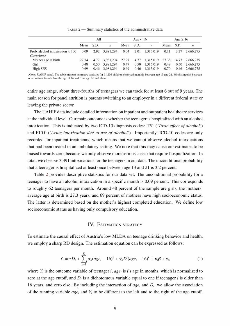
Table 2 — Summary statistics of the administrative data

All Age < 16 Age ≥ 16

Mean S.D. n Mean S.D. n Mean S.D. n

Prob. alcohol intoxication × 100 0.09 2.92 3,981,294 0.04 2.01 1,315,019 0.11 3.27 2,666,275Covariates

Mother age at birth 27.34 4.77 3,981,294 27.27 4.77 1,315,019 27.38 4.77 2,666,275Girl 0.48 0.50 3,981,294 0.49 0.50 1,315,019 0.48 0.50 2,666,275High SES 0.69 0.46 3,981,294 0.69 0.46 1,315,019 0.70 0.46 2,666,275

Notes: UAHIF panel. The table presents summary statistics for 91,208 children observed monthly between age 13 and 21. We distinguish betweenobservations from below the age of 16 and from age 16 and above.

entire age range, about three-fourths of teenagers we can track for at least 6 out of 9 years. Themain reason for panel attrition is parents switching to an employer in a different federal state orleaving the private sector.

The UAHIF data include detailed information on inpatient and outpatient healthcare servicesat the individual level. Our main outcome is whether the teenager is hospitalized with an alcoholintoxication. This is indicated by two ICD-10 diagnosis codes: T51 (’Toxic effect of alcohol’)and F10.0 (’Acute intoxication due to use of alcohol’). Importantly, ICD-10 codes are onlyrecorded for inpatient treatments, which means that we cannot observe alcohol intoxicationsthat had been treated in an ambulatory setting. We note that this may cause our estimates to bebiased towards zero, because we only observe more serious cases that require hospitalization. Intotal, we observe 3,391 intoxications for the teenagers in our data. The unconditional probabilitythat a teenager is hospitalized at least once between age 13 and 21 is 3.2 percent.

Table 2 provides descriptive statistics for our data set. The unconditional probability for ateenager to have an alcohol intoxication in a specific month is 0.09 percent. This correspondsto roughly 62 teenagers per month. Around 48 percent of the sample are girls, the mothers’average age at birth is 27.3 years, and 69 percent of mothers have high socioeconomic status.The latter is determined based on the mother’s highest completed education. We define lowsocioeconomic status as having only compulsory education.

IV. Estimation strategy

To estimate the causal effect of Austria’s low MLDA on teenage drinking behavior and health,we employ a sharp RD design. The estimation equation can be expressed as follows:

Yi = τDi +

K∑k=1

αk(agei − 16)k + γkDi(agei − 16)k + xiβ + εi, (1)

where Yi is the outcome variable of teenager i, agei is i’s age in months, which is normalized tozero at the age cutoff, and Di is a dichotomous variable equal to one if teenager i is older than16 years, and zero else. By including the interaction of agei and Di, we allow the associationof the running variable agei and Yi to be different to the left and to the right of the age cutoff.

9

Finally, xi comprises a set of covariates specified in the results section, and εi is a mean zeroerror term. Standard errors are clustered at the age (in months) level.

The parameter τ identifies the causal effect of the low MLDA under the assumption thattreatment status jumps deterministically and discretely at the threshold of 16 years, whereas allother determinants of Yi run smoothly across the age threshold. The MLDA laws clearly statethat in all Austrian states teenagers gain legal access to non-distilled alcohol at their 16th birth-day, i.e., treatment jumps deterministically and discretely at age 16. However, we have to makesure that we assign adolescents correctly to the left or to the right of the MLDA threshold. Thismeans that we need to precisely measure the teenagers’ age. The administrative data allow usto do so since we have information on the exact date of birth and the exact date of any hospital-ization with acute alcohol intoxication for all adolescents. Yet, in the ESPAD survey data, weonly know the participants’ year and month of birth. To avoid wrong treatment assignment, wedrop all teenagers who turn 16 at some (unknown) day in the month of the ESPAD interview.

Lee and Lemieux (2010) discuss RD settings like ours that exploit discontinuities in agewith inevitable treatment. Three points are worth discussing. First, since all individuals gettreated at age 16, our RD approach does not allow for estimating long-run effects of the MLDA.Second, since we observe the same individuals over time in our administrative panel data set,any balance tests would not be meaningful. Third, and probably most importantly, we wouldoverestimate the effect of gaining legal access to alcohol if teenagers systematically reduceddrinking in the last weeks prior to their 16th birthday. As we will show later, we do not find anyevidence for such behavior. Fourth, there are no other regulations (other than MLDA) whichcan cause a discontinuity in alcohol-related outcomes. The legal age to drive a car is 18, and todrive a moped 15. Compulsory schooling ends after nine grades, when students are about 15years of age. Smoking was legal at 16 during our sample period (now 18). However, based onESPAD data we do not find any evidence for an increase in smoking at age 16, neither at theextensive nor at the intensive margin. Therefore, we are confident that we identify an unbiasedeffect of the MLDA on alcohol consumption and immediate health consequences in our RDapproach.

V. Results

V.1. Effects on drinking behavior

In a first step, we investigate by how much the frequency of consuming alcohol changes whengaining legal access at age 16. To this end, we make use of detailed information provided byteenagers in the ESPAD survey. In particular, respondents report on how many of the last sevendays they drank alcohol. We use this information as the outcome variable in our RD model.Table 3 shows the results from this analysis.

In column (1) of Table 3, we start with a basic RD linear spline specification and find that

10

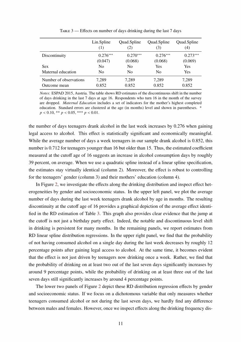
Table 3 — Effects on number of days drinking during the last 7 days

Lin.Spline Quad.Spline Quad.Spline Quad.Spline(1) (2) (3) (4)

Discontinuity 0.276∗∗∗ 0.270∗∗∗ 0.276∗∗∗ 0.273∗∗∗

(0.047) (0.068) (0.068) (0.069)Sex No No Yes YesMaternal education No No No Yes

Number of observations 7,289 7,289 7,289 7,289Outcome mean 0.852 0.852 0.852 0.852

Notes: ESPAD 2015, Austria. The table shows RD estimates of the discontinuous shift in the numberof days drinking in the last 7 days at age 16. Respondents who turn 16 in the month of the surveyare dropped. Maternal Education includes a set of indicators for the mother’s highest completededucation. Standard errors are clustered at the age (in months) level and shown in parentheses. *p < 0.10, ** p < 0.05, *** p < 0.01.

the number of days teenagers drank alcohol in the last week increases by 0.276 when gaininglegal access to alcohol. This effect is statistically significant and economically meaningful.While the average number of days a week teenagers in our sample drank alcohol is 0.852, thisnumber is 0.712 for teenagers younger than 16 but older than 15. Thus, the estimated coefficientmeasured at the cutoff age of 16 suggests an increase in alcohol consumption days by roughly39 percent, on average. When we use a quadratic spline instead of a linear spline specification,the estimates stay virtually identical (column 2). Moreover, the effect is robust to controllingfor the teenagers’ gender (column 3) and their mothers’ education (column 4).

In Figure 2, we investigate the effects along the drinking distribution and inspect effect het-erogeneities by gender and socioeconomic status. In the upper left panel, we plot the averagenumber of days during the last week teenagers drank alcohol by age in months. The resultingdiscontinuity at the cutoff age of 16 provides a graphical depiction of the average effect identi-fied in the RD estimation of Table 3. This graph also provides clear evidence that the jump atthe cutoff is not just a birthday party effect. Indeed, the notable and discontinuous level shiftin drinking is persistent for many months. In the remaining panels, we report estimates fromRD linear spline distribution regressions. In the upper right panel, we find that the probabilityof not having consumed alcohol on a single day during the last week decreases by roughly 12percentage points after gaining legal access to alcohol. At the same time, it becomes evidentthat the effect is not just driven by teenagers now drinking once a week. Rather, we find thatthe probability of drinking on at least two out of the last seven days significantly increases byaround 9 percentage points, while the probability of drinking on at least three out of the lastseven days still significantly increases by around 4 percentage points.

The lower two panels of Figure 2 depict these RD distribution regression effects by genderand socioeconomic status. If we focus on a dichotomous variable that only measures whetherteenagers consumed alcohol or not during the last seven days, we hardly find any differencebetween males and females. However, once we inspect effects along the drinking frequency dis-

11

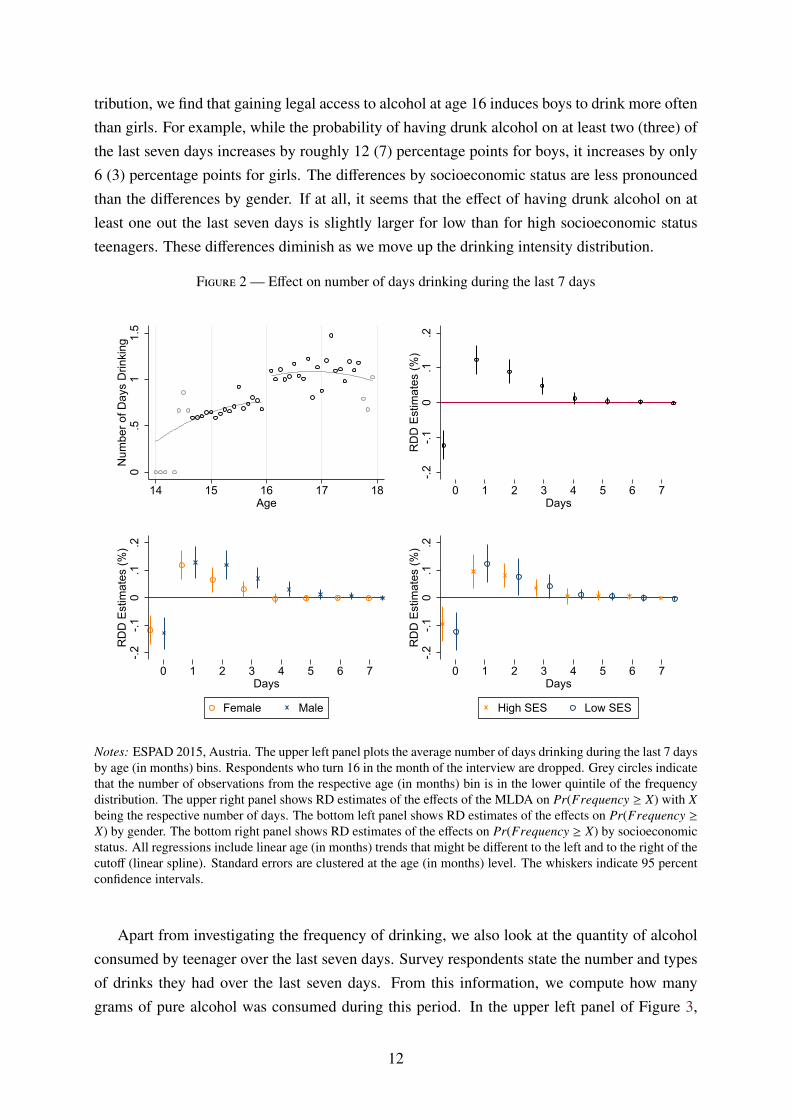
tribution, we find that gaining legal access to alcohol at age 16 induces boys to drink more oftenthan girls. For example, while the probability of having drunk alcohol on at least two (three) ofthe last seven days increases by roughly 12 (7) percentage points for boys, it increases by only6 (3) percentage points for girls. The differences by socioeconomic status are less pronouncedthan the differences by gender. If at all, it seems that the effect of having drunk alcohol on atleast one out the last seven days is slightly larger for low than for high socioeconomic statusteenagers. These differences diminish as we move up the drinking intensity distribution.

Figure 2 — Effect on number of days drinking during the last 7 days

0.5

11.

5N

umbe

r of D

ays

Drin

king

14 15 16 17 18Age

-.2-.1

0.1

.2R

DD

Est

imat

es (%

)

0 1 2 3 4 5 6 7Days

-.2-.1

0.1

.2R

DD

Est

imat

es (%

)

0 1 2 3 4 5 6 7Days

Female Male

-.2-.1

0.1

.2R

DD

Est

imat

es (%

)

0 1 2 3 4 5 6 7Days

High SES Low SES

Notes: ESPAD 2015, Austria. The upper left panel plots the average number of days drinking during the last 7 daysby age (in months) bins. Respondents who turn 16 in the month of the interview are dropped. Grey circles indicatethat the number of observations from the respective age (in months) bin is in the lower quintile of the frequencydistribution. The upper right panel shows RD estimates of the effects of the MLDA on Pr(Frequency ≥ X) with Xbeing the respective number of days. The bottom left panel shows RD estimates of the effects on Pr(Frequency ≥X) by gender. The bottom right panel shows RD estimates of the effects on Pr(Frequency ≥ X) by socioeconomicstatus. All regressions include linear age (in months) trends that might be different to the left and to the right of thecutoff (linear spline). Standard errors are clustered at the age (in months) level. The whiskers indicate 95 percentconfidence intervals.

Apart from investigating the frequency of drinking, we also look at the quantity of alcoholconsumed by teenager over the last seven days. Survey respondents state the number and typesof drinks they had over the last seven days. From this information, we compute how manygrams of pure alcohol was consumed during this period. In the upper left panel of Figure 3,

12

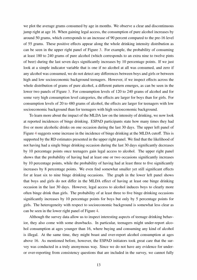
we plot the average grams consumed by age in months. We observe a clear and discontinuousjump right at age 16. When gaining legal access, the consumption of pure alcohol increases byaround 50 grams, which corresponds to an increase of 90 percent compared to the pre-16 levelof 55 grams. These positive effects appear along the whole drinking intensity distribution ascan be seen in the upper right panel of Figure 3. For example, the probability of consumingat least 180 to 240 grams of pure alcohol (which corresponds to an extra nine to twelve pintsof beer) during the last seven days significantly increases by 10 percentage points. If we justlook at a simple indicator variable that is one if no alcohol at all was consumed, and zero ifany alcohol was consumed, we do not detect any differences between boys and girls or betweenhigh and low socioeconomic background teenagers. However, if we inspect effects across thewhole distribution of grams of pure alcohol, a different pattern emerges, as can be seen in thelower two panels of Figure 3. For consumption levels of 120 to 240 grams of alcohol and forsome very high consumption level categories, the effects are larger for boys than for girls. Forconsumption levels of 20 to 480 grams of alcohol, the effects are larger for teenagers with lowsocioeconomic background than for teenagers with high socioeconomic background.

To learn more about the impact of the MLDA law on the intensity of drinking, we now lookat reported incidences of binge drinking. ESPAD participants state how many times they hadfive or more alcoholic drinks on one occasion during the last 30 days. The upper left panel ofFigure 4 suggests some increase in the incidence of binge drinking at the MLDA cutoff. This issupported by the RD estimates presented in the upper right panel. We find that the likelihood ofnot having had a single binge drinking occasion during the last 30 days significantly decreasesby 10 percentage points once teenagers gain legal access to alcohol. The upper right panelshows that the probability of having had at least one or two occasions significantly increasesby 10 percentage points, while the probability of having had at least three to five significantlyincreases by 8 percentage points. We even find somewhat smaller yet still significant effectsfor at least six to nine binge drinking occasions. The graph in the lower left panel showsthat boys and girls do not differ in the MLDA effect of having at least one binge drinkingoccasion in the last 30 days. However, legal access to alcohol induces boys to clearly moreoften binge drink than girls. The probability of at least three to five binge drinking occasionssignificantly increases by 10 percentage points for boys but only by 5 percentage points forgirls. The heterogeneity with respect to socioeconomic background is somewhat less clear ascan be seen in the lower right panel of Figure 4.

Although the survey data allow us to inspect interesting aspects of teenage drinking behav-ior, they also come with some drawbacks. In particular, teenagers might under-report alco-hol consumption at ages younger than 16, where buying and consuming any kind of alcoholis illegal. At the same time, they might boast and over-report alcohol consumption at agesabove 16. As mentioned before, however, the ESPAD initiators took great care that the sur-vey was conducted in a truly anonymous way. Since we do not have any evidence for under-or over-reporting from consistency questions that are included in the survey, we cannot fully

13

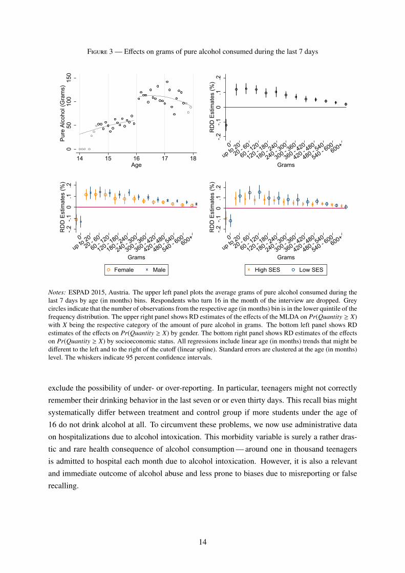
Figure 3 — Effects on grams of pure alcohol consumed during the last 7 days

050

100

150

Pure

Alc

ohol

(Gra

ms)

14 15 16 17 18Age

-.2-.1

0.1

.2R

DD

Est

imat

es (%

)

0

up to 2020 - 6

0

60 - 120

120 - 180

180 - 240

240 - 300

300 - 360

360 - 420

420 - 480

480 - 540

540 - 600

600+

Grams

-.2-.1

0.1

.2R

DD

Est

imat

es (%

)

0

up to 2020 - 6

0

60 - 120

120 - 180

180 - 240

240 - 300

300 - 360

360 - 420

420 - 480

480 - 540

540 - 600

600+

Grams

Female Male

-.2-.1

0.1

.2R

DD

Est

imat

es (%

)

0

up to 2020 - 6

0

60 - 120

120 - 180

180 - 240

240 - 300

300 - 360

360 - 420

420 - 480

480 - 540

540 - 600

600+

Grams

High SES Low SES

Notes: ESPAD 2015, Austria. The upper left panel plots the average grams of pure alcohol consumed during thelast 7 days by age (in months) bins. Respondents who turn 16 in the month of the interview are dropped. Greycircles indicate that the number of observations from the respective age (in months) bin is in the lower quintile of thefrequency distribution. The upper right panel shows RD estimates of the effects of the MLDA on Pr(Quantity ≥ X)with X being the respective category of the amount of pure alcohol in grams. The bottom left panel shows RDestimates of the effects on Pr(Quantity ≥ X) by gender. The bottom right panel shows RD estimates of the effectson Pr(Quantity ≥ X) by socioeconomic status. All regressions include linear age (in months) trends that might bedifferent to the left and to the right of the cutoff (linear spline). Standard errors are clustered at the age (in months)level. The whiskers indicate 95 percent confidence intervals.

exclude the possibility of under- or over-reporting. In particular, teenagers might not correctlyremember their drinking behavior in the last seven or or even thirty days. This recall bias mightsystematically differ between treatment and control group if more students under the age of16 do not drink alcohol at all. To circumvent these problems, we now use administrative dataon hospitalizations due to alcohol intoxication. This morbidity variable is surely a rather dras-tic and rare health consequence of alcohol consumption — around one in thousand teenagersis admitted to hospital each month due to alcohol intoxication. However, it is also a relevantand immediate outcome of alcohol abuse and less prone to biases due to misreporting or falserecalling.

14

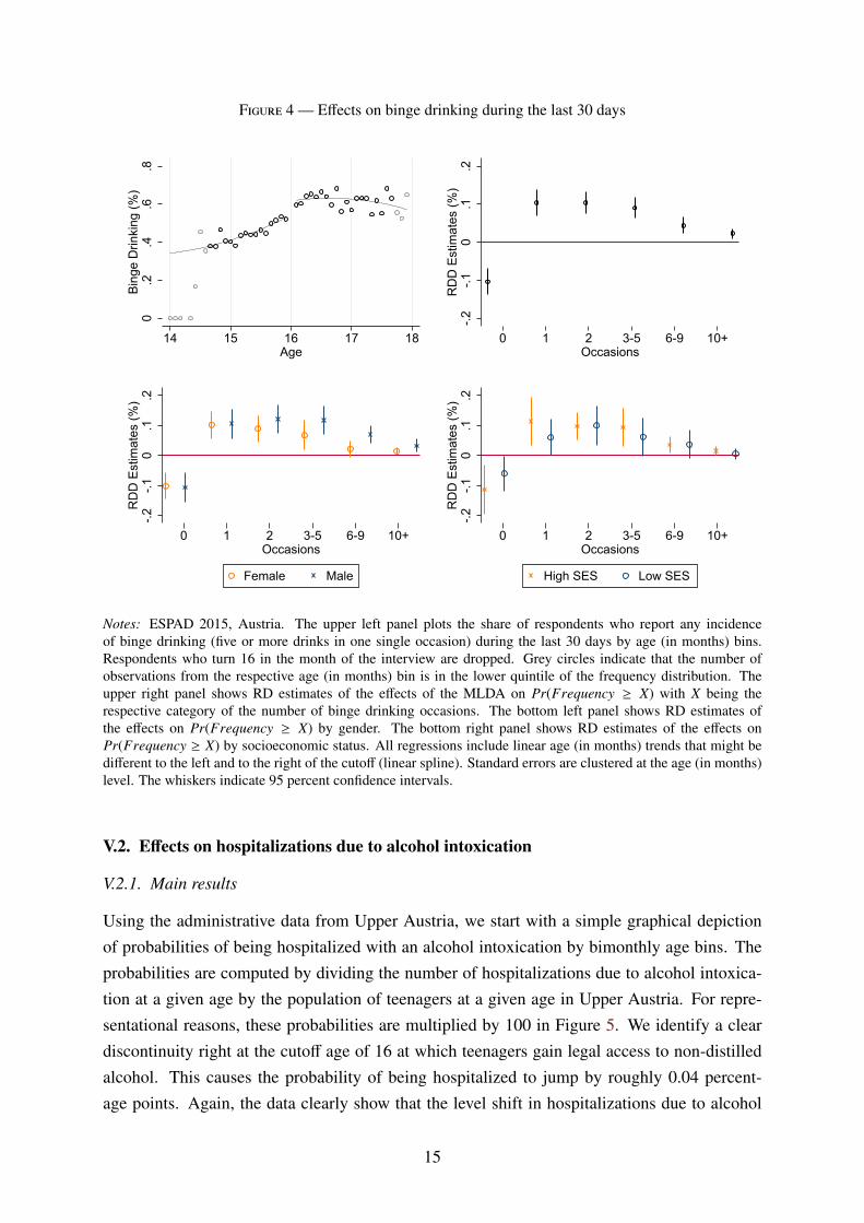
Figure 4 — Effects on binge drinking during the last 30 days

0.2

.4.6

.8Bi

nge

Drin

king

(%)

14 15 16 17 18Age

-.2-.1

0.1

.2R

DD

Est

imat

es (%

)

0 1 2 3-5 6-9 10+Occasions

-.2-.1

0.1

.2R

DD

Est

imat

es (%

)

0 1 2 3-5 6-9 10+Occasions

Female Male

-.2-.1

0.1

.2R

DD

Est

imat

es (%

)

0 1 2 3-5 6-9 10+Occasions

High SES Low SES

Notes: ESPAD 2015, Austria. The upper left panel plots the share of respondents who report any incidenceof binge drinking (five or more drinks in one single occasion) during the last 30 days by age (in months) bins.Respondents who turn 16 in the month of the interview are dropped. Grey circles indicate that the number ofobservations from the respective age (in months) bin is in the lower quintile of the frequency distribution. Theupper right panel shows RD estimates of the effects of the MLDA on Pr(Frequency ≥ X) with X being therespective category of the number of binge drinking occasions. The bottom left panel shows RD estimates ofthe effects on Pr(Frequency ≥ X) by gender. The bottom right panel shows RD estimates of the effects onPr(Frequency ≥ X) by socioeconomic status. All regressions include linear age (in months) trends that might bedifferent to the left and to the right of the cutoff (linear spline). Standard errors are clustered at the age (in months)level. The whiskers indicate 95 percent confidence intervals.

V.2. Effects on hospitalizations due to alcohol intoxication

V.2.1. Main results

Using the administrative data from Upper Austria, we start with a simple graphical depictionof probabilities of being hospitalized with an alcohol intoxication by bimonthly age bins. Theprobabilities are computed by dividing the number of hospitalizations due to alcohol intoxica-tion at a given age by the population of teenagers at a given age in Upper Austria. For repre-sentational reasons, these probabilities are multiplied by 100 in Figure 5. We identify a cleardiscontinuity right at the cutoff age of 16 at which teenagers gain legal access to non-distilledalcohol. This causes the probability of being hospitalized to jump by roughly 0.04 percent-age points. Again, the data clearly show that the level shift in hospitalizations due to alcohol

15

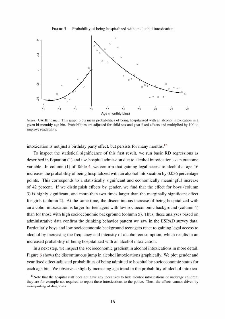
Figure 5 — Probability of being hospitalized with an alcohol intoxication

.06

.08

.1.1

2.1

4

13 14 15 16 17 18 19 20 21 22

Age (monthly bins)

Notes: UAHIF panel. This graph plots mean probabilities of being hospitalized with an alcohol intoxication in agiven bi-monthly age bin. Probabilities are adjusted for child sex and year fixed effects and multiplied by 100 toimprove readability.

intoxication is not just a birthday party effect, but persists for many months.12

To inspect the statistical significance of this first result, we run basic RD regressions asdescribed in Equation (1) and use hospital admission due to alcohol intoxication as an outcomevariable. In column (1) of Table 4, we confirm that gaining legal access to alcohol at age 16increases the probability of being hospitalized with an alcohol intoxication by 0.036 percentagepoints. This corresponds to a statistically significant and economically meaningful increaseof 42 percent. If we distinguish effects by gender, we find that the effect for boys (column3) is highly significant, and more than two times larger than the marginally significant effectfor girls (column 2). At the same time, the discontinuous increase of being hospitalized withan alcohol intoxication is larger for teenagers with low socioeconomic background (column 4)than for those with high socioeconomic background (column 5). Thus, these analyses based onadministrative data confirm the drinking behavior pattern we saw in the ESPAD survey data.Particularly boys and low socioeconomic background teenagers react to gaining legal access toalcohol by increasing the frequency and intensity of alcohol consumption, which results in anincreased probability of being hospitalized with an alcohol intoxication.

In a next step, we inspect the socioeconomic gradient in alcohol intoxications in more detail.Figure 6 shows the discontinuous jump in alcohol intoxications graphically. We plot gender andyear fixed effect-adjusted probabilities of being admitted to hospital by socioeconomic status foreach age bin. We observe a slightly increasing age trend in the probability of alcohol intoxica-

12Note that the hospital staff does not have any incentives to hide alcohol intoxications of underage children;they are for example not required to report these intoxications to the police. Thus, the effects cannot driven bymisreporting of diagnoses.

16

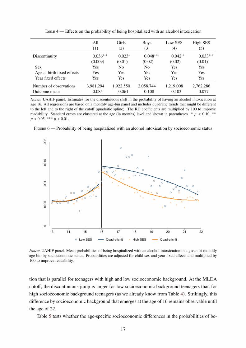
Table 4 — Effects on the probability of being hospitalized with an alcohol intoxication

All Girls Boys Low SES High SES(1) (2) (3) (4) (5)

Discontinuity 0.036∗∗∗ 0.023∗ 0.048∗∗∗ 0.042∗∗ 0.033∗∗∗

(0.009) (0.01) (0.02) (0.02) (0.01)Sex Yes No No Yes YesAge at birth fixed effects Yes Yes Yes Yes YesYear fixed effects Yes Yes Yes Yes Yes

Number of observations 3,981,294 1,922,550 2,058,744 1,219,008 2,762,286Outcome mean 0.085 0.061 0.108 0.103 0.077

Notes: UAHIF panel. Estimates for the discontinuous shift in the probability of having an alcohol intoxication atage 16. All regressions are based on a monthly age-bin panel and includes quadratic trends that might be differentto the left and to the right of the cutoff (quadratic spline). The RD coefficients are multiplied by 100 to improvereadability. Standard errors are clustered at the age (in months) level and shown in parentheses. * p < 0.10, **p < 0.05, *** p < 0.01.

Figure 6 — Probability of being hospitalized with an alcohol intoxication by socioeconomic status

0.0

005

.001

.001

5.0

02

13 14 15 16 17 18 19 20 21 22

Low SES Quadratic fit High SES Quadratic fit

Notes: UAHIF panel. Mean probabilities of being hospitalized with an alcohol intoxication in a given bi-monthlyage bin by socioeconomic status. Probabilities are adjusted for child sex and year fixed effects and multiplied by100 to improve readability.

tion that is parallel for teenagers with high and low socioeconomic background. At the MLDAcutoff, the discontinuous jump is larger for low socioeconomic background teenagers than forhigh socioeconomic background teenagers (as we already know from Table 4). Strikingly, thisdifference by socioeconomic background that emerges at the age of 16 remains observable untilthe age of 22.

Table 5 tests whether the age-specific socioeconomic differences in the probabilities of be-

17

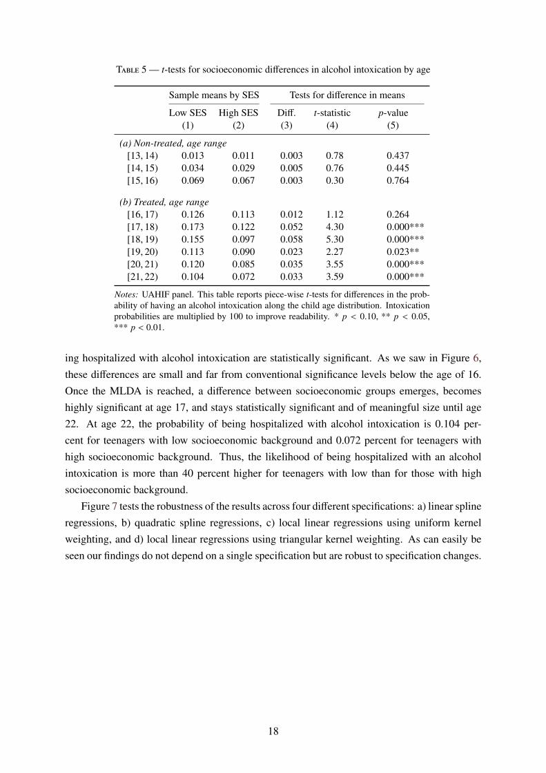
Table 5 — t-tests for socioeconomic differences in alcohol intoxication by age

Sample means by SES Tests for difference in means

Low SES High SES Diff. t-statistic p-value(1) (2) (3) (4) (5)

(a) Non-treated, age range[13, 14) 0.013 0.011 0.003 0.78 0.437[14, 15) 0.034 0.029 0.005 0.76 0.445[15, 16) 0.069 0.067 0.003 0.30 0.764

(b) Treated, age range[16, 17) 0.126 0.113 0.012 1.12 0.264[17, 18) 0.173 0.122 0.052 4.30 0.000***[18, 19) 0.155 0.097 0.058 5.30 0.000***[19, 20) 0.113 0.090 0.023 2.27 0.023**[20, 21) 0.120 0.085 0.035 3.55 0.000***[21, 22) 0.104 0.072 0.033 3.59 0.000***

Notes: UAHIF panel. This table reports piece-wise t-tests for differences in the prob-ability of having an alcohol intoxication along the child age distribution. Intoxicationprobabilities are multiplied by 100 to improve readability. * p < 0.10, ** p < 0.05,*** p < 0.01.

ing hospitalized with alcohol intoxication are statistically significant. As we saw in Figure 6,these differences are small and far from conventional significance levels below the age of 16.Once the MLDA is reached, a difference between socioeconomic groups emerges, becomeshighly significant at age 17, and stays statistically significant and of meaningful size until age22. At age 22, the probability of being hospitalized with alcohol intoxication is 0.104 per-cent for teenagers with low socioeconomic background and 0.072 percent for teenagers withhigh socioeconomic background. Thus, the likelihood of being hospitalized with an alcoholintoxication is more than 40 percent higher for teenagers with low than for those with highsocioeconomic background.

Figure 7 tests the robustness of the results across four different specifications: a) linear splineregressions, b) quadratic spline regressions, c) local linear regressions using uniform kernelweighting, and d) local linear regressions using triangular kernel weighting. As can easily beseen our findings do not depend on a single specification but are robust to specification changes.

18

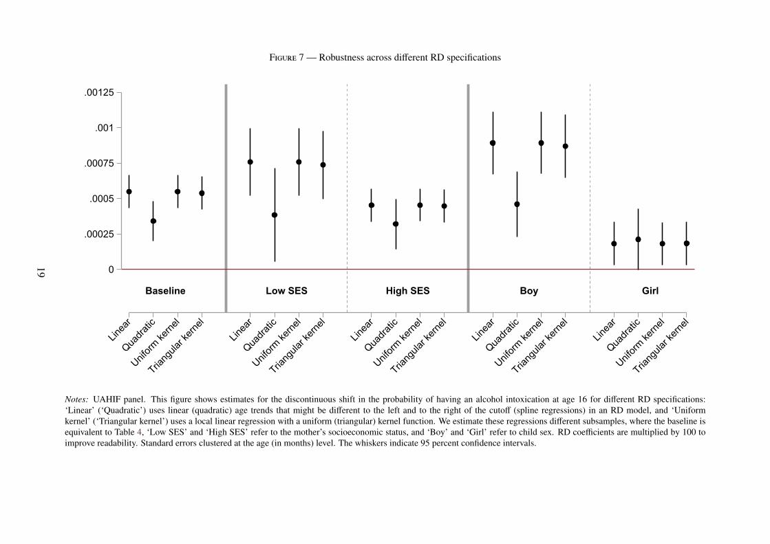
Figure 7 — Robustness across different RD specifications

Baseline Low SES High SES Boy Girl

0

.00025

.0005

.00075

.001

.00125

Linea

rQua

dratic

Uniform

kerne

l

Triang

ular k

ernel

Linea

rQua

dratic

Uniform

kerne

l

Triang

ular k

ernel

Linea

rQua

dratic

Uniform

kerne

l

Triang

ular k

ernel

Linea

rQua

dratic

Uniform

kerne

l

Triang

ular k

ernel

Linea

rQua

dratic

Uniform

kerne

l

Triang

ular k

ernel

Notes: UAHIF panel. This figure shows estimates for the discontinuous shift in the probability of having an alcohol intoxication at age 16 for different RD specifications:‘Linear’ (‘Quadratic’) uses linear (quadratic) age trends that might be different to the left and to the right of the cutoff (spline regressions) in an RD model, and ‘Uniformkernel’ (‘Triangular kernel’) uses a local linear regression with a uniform (triangular) kernel function. We estimate these regressions different subsamples, where the baseline isequivalent to Table 4, ‘Low SES’ and ‘High SES’ refer to the mother’s socioeconomic status, and ‘Boy’ and ‘Girl’ refer to child sex. RD coefficients are multiplied by 100 toimprove readability. Standard errors clustered at the age (in months) level. The whiskers indicate 95 percent confidence intervals.

19

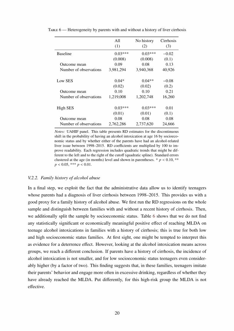
Table 6 — Heterogeneity by parents with and without a history of liver cirrhosis

All No history Cirrhosis(1) (2) (3)

Baseline 0.03*** 0.03*** −0.02(0.008) (0.008) (0.1)

Outcome mean 0.09 0.08 0.13Number of observations 3,981,294 3,940,368 40,926

Low SES 0.04* 0.04** −0.08(0.02) (0.02) (0.2)

Outcome mean 0.10 0.10 0.21Number of observations 1,219,008 1,202,748 16,260

High SES 0.03*** 0.03*** 0.01(0.01) (0.01) (0.1)

Outcome mean 0.08 0.08 0.08Number of observations 2,762,286 2,737,620 24,666

Notes: UAHIF panel. This table presents RD estimates for the discontinuousshift in the probability of having an alcohol intoxication at age 16 by socioeco-nomic status and by whether either of the parents have had an alcohol-relatedliver issue between 1998–2015. RD coefficients are multiplied by 100 to im-prove readability. Each regression includes quadratic trends that might be dif-ferent to the left and to the right of the cutoff (quadratic spline). Standard errorsclustered at the age (in months) level and shown in parentheses. * p < 0.10, **p < 0.05, *** p < 0.01.

V.2.2. Family history of alcohol abuse

In a final step, we exploit the fact that the administrative data allow us to identify teenagerswhose parents had a diagnosis of liver cirrhosis between 1998–2015. This provides us with agood proxy for a family history of alcohol abuse. We first run the RD regressions on the wholesample and distinguish between families with and without a recent history of cirrhosis. Then,we additionally split the sample by socioeconomic status. Table 6 shows that we do not findany statistically significant or economically meaningful positive effect of reaching MLDA onteenage alcohol intoxications in families with a history of cirrhosis; this is true for both lowand high socioeconomic status families. At first sight, one might be tempted to interpret thisas evidence for a deterrence effect. However, looking at the alcohol intoxication means acrossgroups, we reach a different conclusion. If parents have a history of cirrhosis, the incidence ofalcohol intoxication is not smaller, and for low socioeconomic status teenagers even consider-ably higher (by a factor of two). This finding suggests that, in these families, teenagers imitatetheir parents’ behavior and engage more often in excessive drinking, regardless of whether theyhave already reached the MLDA. Put differently, for this high-risk group the MLDA is noteffective.

20

V.2.3. Substitution behavior and spillovers to other risky behavior

A large literature discusses whether alcohol is a substitute for or a complement to other riskyactivities, such as drug use. Figure A.2 in the Appendix shows RD estimates of reaching theMLDA on a set of additional health outcomes ranging from injuries and sexually transmit-table diseases to drug prescriptions and drug-related treatments; again, we distinguish betweenteenagers from low and high socioeconomic status families. We do not find any robust evidencefor a meaningful impact of the MLDA (and the associated increase in alcohol consumption) onhealth outcomes other than alcohol intoxication.

V.3. Effects on access to alcohol and risk perceptions

The discontinuous increase in alcohol consumption at the age of 16 shows that MLDA legisla-tion is successful in preventing many (but not all) underage children from consuming alcohol. Inthis section, we aim at providing evidence on the underlying mechanism. One obvious channelis restricted physical access to alcohol. We have two data sources to evaluate the importance ofthis channel. First, we use data from an annual large-scale field study, which sends underage testbuyers to retailers to buy alcohol.13 Second, we use ESPAD survey responses on perceived ac-cess. The former provide us with objective information on alcohol access at retailers, while thelatter refers to self-reported overall access, including access provided by siblings and friends.In a final step, we discuss normative values imposed by alcohol legislation as an additionalchannel. To this end, we use survey questions on risk perceptions about alcohol as a proxyoutcome.

V.3.1. Objective access at retailers

Since 2014, the Upper Austrian government has commissioned the main addiction preventioncenter (Institut Suchtprävention – pro Mente Oberösterreich) to annually organize a large num-ber of underage alcohol purchase attempts across Upper Austria. The test buyers are all underthe age of 16. They are trained by experts and accompanied by adult custodians during theprocedure. The test purchases were carried out in grocery stores, in petrol station shops, andin restaurants across Upper Austria; the test shoppers were instructed to buy a 0.7 liter bottleof hard liquor (Vodka). Since access to hard liquor is legally restricted up to age 18 in UpperAustria, the success rates of test shoppers represent a lower bound of the success rates we wouldexpect for non-distilled alcohol such as beer and wine.14 We have access to anonymized microdata on all purchase attempts (except restaurants). Our dataset includes information on the dateand place of 4,269 purchase attempts.

13This is a common method to check the compliance with restrictions on alcohol sales (see, e.g., Gosselt et al.,2007).

14Further details on the survey are available here: https://www.praevention.at/jugend/testkaeufe-jugendschutz

21

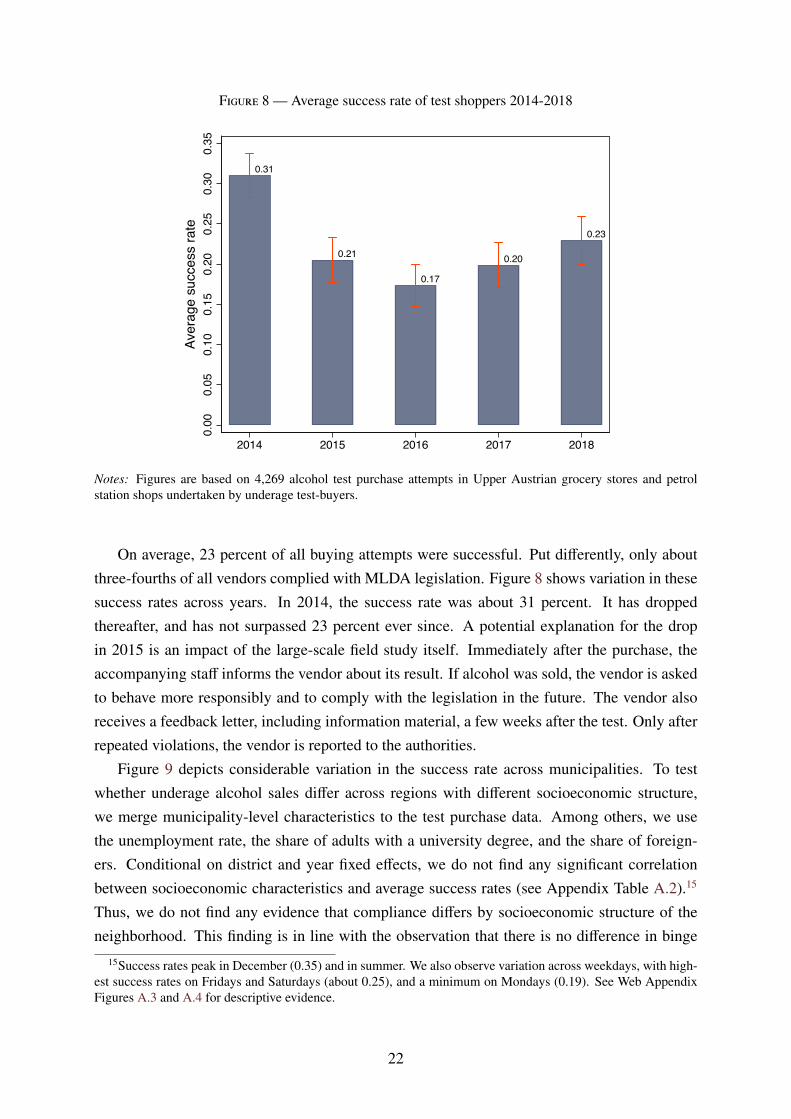
Figure 8 — Average success rate of test shoppers 2014-2018

0.31

0.21

0.17

0.20

0.23

0.00

0.05

0.10

0.15

0.20

0.25

0.30

0.35

Aver

age

succ

ess

rate

2014 2015 2016 2017 2018

Notes: Figures are based on 4,269 alcohol test purchase attempts in Upper Austrian grocery stores and petrolstation shops undertaken by underage test-buyers.

On average, 23 percent of all buying attempts were successful. Put differently, only aboutthree-fourths of all vendors complied with MLDA legislation. Figure 8 shows variation in thesesuccess rates across years. In 2014, the success rate was about 31 percent. It has droppedthereafter, and has not surpassed 23 percent ever since. A potential explanation for the dropin 2015 is an impact of the large-scale field study itself. Immediately after the purchase, theaccompanying staff informs the vendor about its result. If alcohol was sold, the vendor is askedto behave more responsibly and to comply with the legislation in the future. The vendor alsoreceives a feedback letter, including information material, a few weeks after the test. Only afterrepeated violations, the vendor is reported to the authorities.

Figure 9 depicts considerable variation in the success rate across municipalities. To testwhether underage alcohol sales differ across regions with different socioeconomic structure,we merge municipality-level characteristics to the test purchase data. Among others, we usethe unemployment rate, the share of adults with a university degree, and the share of foreign-ers. Conditional on district and year fixed effects, we do not find any significant correlationbetween socioeconomic characteristics and average success rates (see Appendix Table A.2).15

Thus, we do not find any evidence that compliance differs by socioeconomic structure of theneighborhood. This finding is in line with the observation that there is no difference in binge

15Success rates peak in December (0.35) and in summer. We also observe variation across weekdays, with high-est success rates on Fridays and Saturdays (about 0.25), and a minimum on Mondays (0.19). See Web AppendixFigures A.3 and A.4 for descriptive evidence.

22

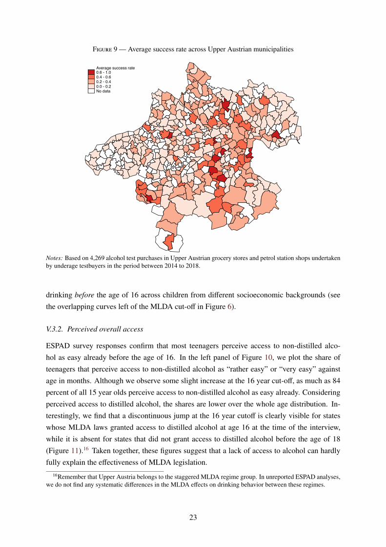
Figure 9 — Average success rate across Upper Austrian municipalities

Average success rate0.6 - 1.00.4 - 0.60.2 - 0.40.0 - 0.2No data

Notes: Based on 4,269 alcohol test purchases in Upper Austrian grocery stores and petrol station shops undertakenby underage testbuyers in the period between 2014 to 2018.

drinking before the age of 16 across children from different socioeconomic backgrounds (seethe overlapping curves left of the MLDA cut-off in Figure 6).

V.3.2. Perceived overall access

ESPAD survey responses confirm that most teenagers perceive access to non-distilled alco-hol as easy already before the age of 16. In the left panel of Figure 10, we plot the share ofteenagers that perceive access to non-distilled alcohol as “rather easy” or “very easy” againstage in months. Although we observe some slight increase at the 16 year cut-off, as much as 84percent of all 15 year olds perceive access to non-distilled alcohol as easy already. Consideringperceived access to distilled alcohol, the shares are lower over the whole age distribution. In-terestingly, we find that a discontinuous jump at the 16 year cutoff is clearly visible for stateswhose MLDA laws granted access to distilled alcohol at age 16 at the time of the interview,while it is absent for states that did not grant access to distilled alcohol before the age of 18(Figure 11).16 Taken together, these figures suggest that a lack of access to alcohol can hardlyfully explain the effectiveness of MLDA legislation.

16Remember that Upper Austria belongs to the staggered MLDA regime group. In unreported ESPAD analyses,we do not find any systematic differences in the MLDA effects on drinking behavior between these regimes.

23

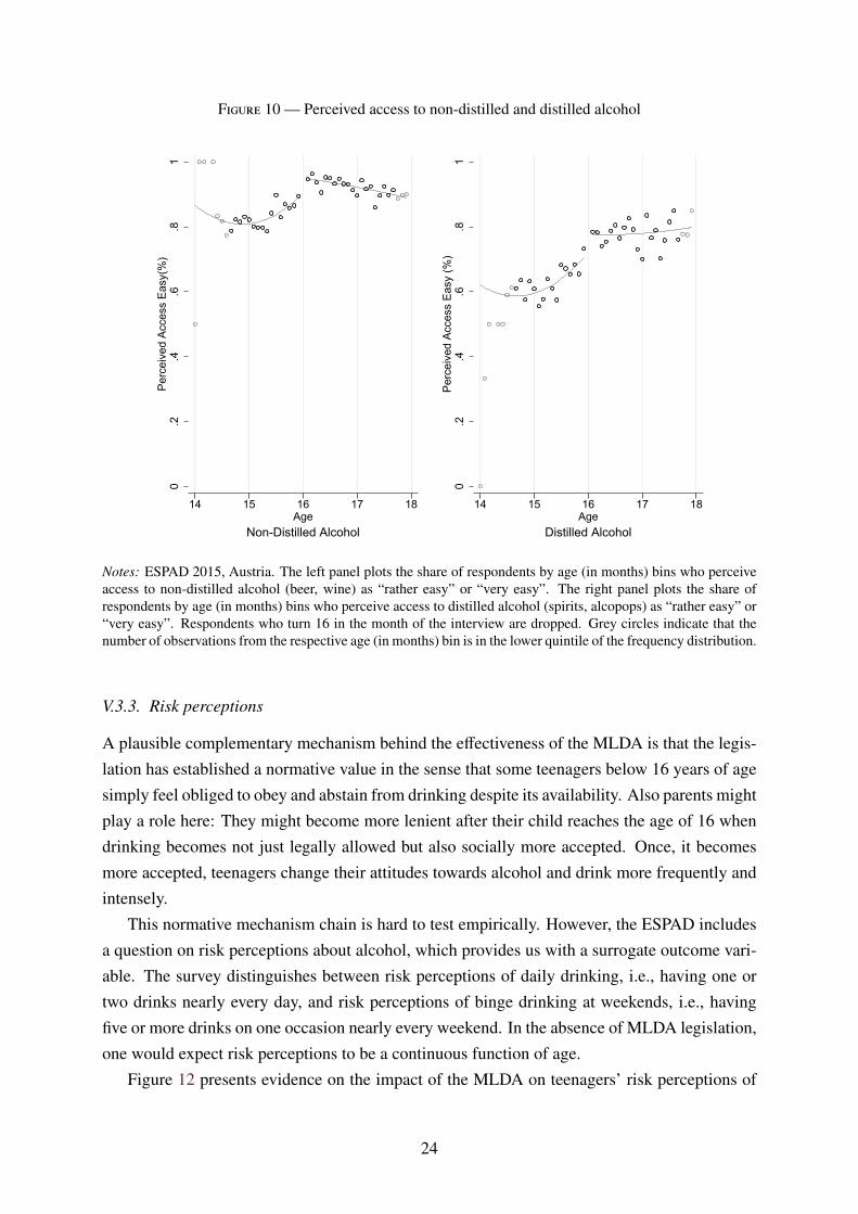
Figure 10 — Perceived access to non-distilled and distilled alcohol

0.2

.4.6

.81

Perc

eive

d Ac

cess

Eas

y(%

)

14 15 16 17 18Age

Non-Distilled Alcohol

0.2

.4.6

.81

Perc

eive

d Ac

cess

Eas

y (%

)

14 15 16 17 18Age

Distilled Alcohol

Notes: ESPAD 2015, Austria. The left panel plots the share of respondents by age (in months) bins who perceiveaccess to non-distilled alcohol (beer, wine) as “rather easy” or “very easy”. The right panel plots the share ofrespondents by age (in months) bins who perceive access to distilled alcohol (spirits, alcopops) as “rather easy” or“very easy”. Respondents who turn 16 in the month of the interview are dropped. Grey circles indicate that thenumber of observations from the respective age (in months) bin is in the lower quintile of the frequency distribution.

V.3.3. Risk perceptions

A plausible complementary mechanism behind the effectiveness of the MLDA is that the legis-lation has established a normative value in the sense that some teenagers below 16 years of agesimply feel obliged to obey and abstain from drinking despite its availability. Also parents mightplay a role here: They might become more lenient after their child reaches the age of 16 whendrinking becomes not just legally allowed but also socially more accepted. Once, it becomesmore accepted, teenagers change their attitudes towards alcohol and drink more frequently andintensely.

This normative mechanism chain is hard to test empirically. However, the ESPAD includesa question on risk perceptions about alcohol, which provides us with a surrogate outcome vari-able. The survey distinguishes between risk perceptions of daily drinking, i.e., having one ortwo drinks nearly every day, and risk perceptions of binge drinking at weekends, i.e., havingfive or more drinks on one occasion nearly every weekend. In the absence of MLDA legislation,one would expect risk perceptions to be a continuous function of age.

Figure 12 presents evidence on the impact of the MLDA on teenagers’ risk perceptions of

24

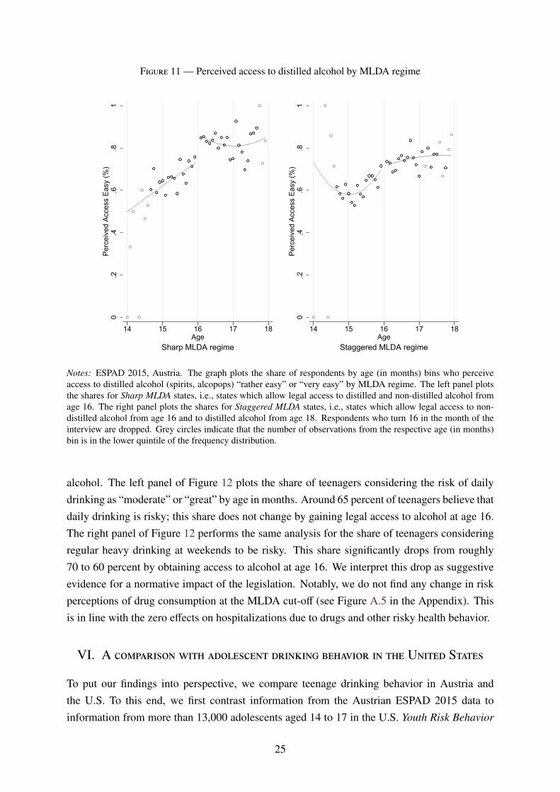
Figure 11 — Perceived access to distilled alcohol by MLDA regime

0.2

.4.6

.81

Perc

eive

d Ac

cess

Eas

y (%

)

14 15 16 17 18Age

Sharp MLDA regime

0.2

.4.6

.81

Perc

eive

d Ac

cess

Eas

y (%

)

14 15 16 17 18Age

Staggered MLDA regime

Notes: ESPAD 2015, Austria. The graph plots the share of respondents by age (in months) bins who perceiveaccess to distilled alcohol (spirits, alcopops) “rather easy” or “very easy” by MLDA regime. The left panel plotsthe shares for Sharp MLDA states, i.e., states which allow legal access to distilled and non-distilled alcohol fromage 16. The right panel plots the shares for Staggered MLDA states, i.e., states which allow legal access to non-distilled alcohol from age 16 and to distilled alcohol from age 18. Respondents who turn 16 in the month of theinterview are dropped. Grey circles indicate that the number of observations from the respective age (in months)bin is in the lower quintile of the frequency distribution.

alcohol. The left panel of Figure 12 plots the share of teenagers considering the risk of dailydrinking as “moderate” or “great” by age in months. Around 65 percent of teenagers believe thatdaily drinking is risky; this share does not change by gaining legal access to alcohol at age 16.The right panel of Figure 12 performs the same analysis for the share of teenagers consideringregular heavy drinking at weekends to be risky. This share significantly drops from roughly70 to 60 percent by obtaining access to alcohol at age 16. We interpret this drop as suggestiveevidence for a normative impact of the legislation. Notably, we do not find any change in riskperceptions of drug consumption at the MLDA cut-off (see Figure A.5 in the Appendix). Thisis in line with the zero effects on hospitalizations due to drugs and other risky health behavior.

VI. A comparison with adolescent drinking behavior in the United States

To put our findings into perspective, we compare teenage drinking behavior in Austria andthe U.S. To this end, we first contrast information from the Austrian ESPAD 2015 data toinformation from more than 13,000 adolescents aged 14 to 17 in the U.S. Youth Risk Behavior

25

Figure 12 — Risk perception of daily drinking and heavy drinking at weekends

0.2

.4.6

.81

Perc

eive

d R

isk

Mod

erat

e/H

igh

(%)

14 15 16 17 18Age

Daily Drinking

0.2

.4.6

.81

Perc

eive

d R

isk

Mod

erat

e/H

igh

(%)

14 15 16 17 18Age

Heavy Drinking on Weekends

Notes: ESPAD 2015, Austria. The graph plots the share of respondents by age (in months) bins who perceive dailydrinking (left panel) or heavy drinking on weekends, i.e., having five or more drinks in one occasion nearly everyweekend (right panel) risky. Respondents who turn 16 in the month of the interview are dropped. Grey circlesindicate that the number of observations from the respective age (in months) bin is in the lower quintile of thefrequency distribution.

Surveillance System 2015 (YRBSS). We investigate two questions on drinking behavior that areconsistently asked across both surveys. The left panel of Figure 13 plots the share of respondentswho report drinking at least once during the last 30 days over age in years for both Austria andthe U.S. The right panel of Figure 13 plots the share of respondents who report at least onebinge drinking incident (meaning five or more alcoholic beverages on one occasion) by age forAustria and the U.S. For both variables, the share is considerably higher in Austria than in theU.S., and this is the case over the entire age spectrum. More than 40 percent of all 14–15 yearolds in Austria report at least one binge drinking incidence during the past 30 days, whereasthis number is around 10 percent in the US After the Austrian MLDA cutoff at 16, we observe adisproportionate increase in the share of teenagers who report drinking or heavy drinking. Thejump at the cutoff in the share of teenagers who report binge drinking is more than two timeslarger in Austria than in the U.S. Appendix Table A.1 shows that the difference in this increaseis highly significant and amounts to 9 percentage points.

Using data from the 2000 to 2006 waves of the National Longitudinal Study of the Youth

1979 (NLSY79), we also inspect the increase in drinking behavior of U.S. youths at the MLDAcutoff at 21 years of age. In contrast to the YRBSS data, the NLSY97 contains information on

26

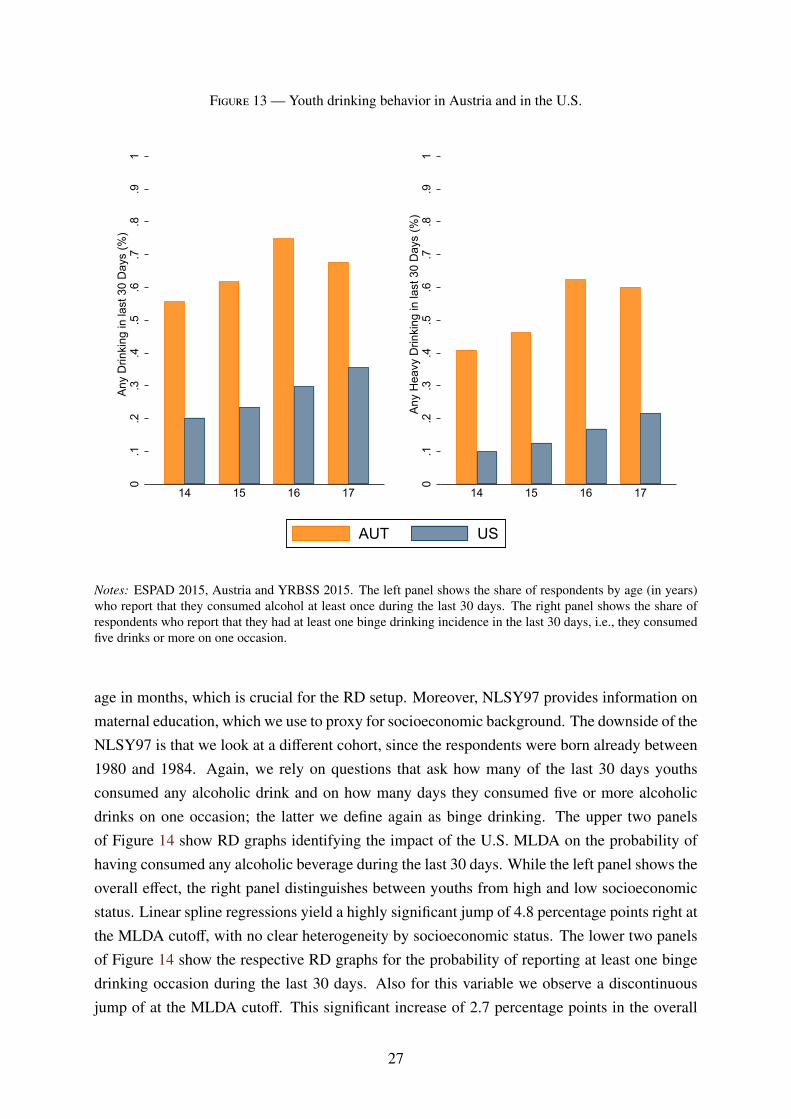
Figure 13 — Youth drinking behavior in Austria and in the U.S.

0.1

.2.3

.4.5

.6.7

.8.9

1An

y D

rinki

ng in

last

30

Day

s (%

)

14 15 16 17

0.1

.2.3

.4.5

.6.7

.8.9

1An

y H

eavy

Drin

king

in la

st 3

0 D

ays

(%)

14 15 16 17

AUT US

Notes: ESPAD 2015, Austria and YRBSS 2015. The left panel shows the share of respondents by age (in years)who report that they consumed alcohol at least once during the last 30 days. The right panel shows the share ofrespondents who report that they had at least one binge drinking incidence in the last 30 days, i.e., they consumedfive drinks or more on one occasion.

age in months, which is crucial for the RD setup. Moreover, NLSY97 provides information onmaternal education, which we use to proxy for socioeconomic background. The downside of theNLSY97 is that we look at a different cohort, since the respondents were born already between1980 and 1984. Again, we rely on questions that ask how many of the last 30 days youthsconsumed any alcoholic drink and on how many days they consumed five or more alcoholicdrinks on one occasion; the latter we define again as binge drinking. The upper two panelsof Figure 14 show RD graphs identifying the impact of the U.S. MLDA on the probability ofhaving consumed any alcoholic beverage during the last 30 days. While the left panel shows theoverall effect, the right panel distinguishes between youths from high and low socioeconomicstatus. Linear spline regressions yield a highly significant jump of 4.8 percentage points right atthe MLDA cutoff, with no clear heterogeneity by socioeconomic status. The lower two panelsof Figure 14 show the respective RD graphs for the probability of reporting at least one bingedrinking occasion during the last 30 days. Also for this variable we observe a discontinuousjump of at the MLDA cutoff. This significant increase of 2.7 percentage points in the overall

27

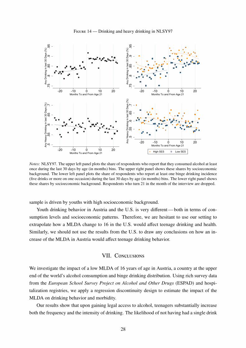
Figure 14 — Drinking and heavy drinking in NLSY97

.75

.8.8

5.9

.95

Any

Drin

king

in la

st 3

0 D

ays

(%)

-20 -10 0 10 20Months To and From Age 21

.75

.8.8

5.9

.95

Any

Drin

king

in la

st 3

0 D

ays

(%)

-20 -10 0 10 20Months To and From Age 21

.5.5

5.6

.65

.7An

y H

eavy

Drin

king

in la

st 3

0 D

ays

(%)

-20 -10 0 10 20Months To and From Age 21

.5.5

5.6

.65

.7An

y H

eavy

Drin

king

in la

st 3

0 D

ays

(%)

-20 -10 0 10 20Months To and From Age 21

High SES Low SES

Notes: NLSY97. The upper left panel plots the share of respondents who report that they consumed alcohol at leastonce during the last 30 days by age (in months) bins. The upper right panel shows these shares by socioeconomicbackground. The lower left panel plots the share of respondents who report at least one binge drinking incidence(five drinks or more on one occasion) during the last 30 days by age (in months) bins. The lower right panel showsthese shares by socioeconomic background. Respondents who turn 21 in the month of the interview are dropped.

sample is driven by youths with high socioeconomic background.Youth drinking behavior in Austria and the U.S. is very different — both in terms of con-

sumption levels and socioeconomic patterns. Therefore, we are hesitant to use our setting toextrapolate how a MLDA change to 16 in the U.S. would affect teenage drinking and health.Similarly, we should not use the results from the U.S. to draw any conclusions on how an in-crease of the MLDA in Austria would affect teenage drinking behavior.

VII. Conclusions

We investigate the impact of a low MLDA of 16 years of age in Austria, a country at the upperend of the world’s alcohol consumption and binge drinking distribution. Using rich survey datafrom the European School Survey Project on Alcohol and Other Drugs (ESPAD) and hospi-talization registries, we apply a regression discontinuity design to estimate the impact of theMLDA on drinking behavior and morbidity.

Our results show that upon gaining legal access to alcohol, teenagers substantially increaseboth the frequency and the intensity of drinking. The likelihood of not having had a single drink

28

over the last seven days shrinks by 12 percentage points. At the same time, the likelihood ofhaving had one to two (three to five) heavy drinking occasions over the last seven days increasesby 10 (8) percentage points. As a consequence, we observe a sharp increase in hospitalizationsdue to alcohol intoxication at the cutoff age of 16. These findings contradict the notion that alow MLDA helps teenagers to ease into drinking (Wechsler and Nelson, 2006).

The effects are stronger for boys and for teenagers with low socioeconomic background. Weshow that the effects persist for some years and cannot be explained by birthday party effects.By the age of 22, the probability of having been hospitalized with an alcohol intoxication is0.104 percent for low socioeconomic background teenagers, and thus 40 percent higher thanfor those with high socioeconomic background.

Investigating the channels, we observe that most teenagers perceive access to alcohol aseasy even before turning 16. Data from large-scale mystery shopping tours suggest that, evenat the points of sale, MLDA enforcement is not very strict. At the same time, we do observe aconspicuous decline in the share of teenagers who consider regular heavy drinking at weekendsrisky right at the MLDA cutoff, while we do not see any change in the share of teenagers whoconsider daily drinking risky. This result might be suggestive evidence in favor of an additionalnormative channel MLDA regulation entails. Some teenagers below 16 years of age may simplyfeel obliged to obey and abstain from drinking, despite its availability. Once drinking becomeslegally allowed and socially acceptable, they change their attitudes towards alcohol and drinkmore frequently and more intensely.

Since we lack adequate data and estimates on the benefits of drinking alcohol at youngage, we cannot perform an encompassing welfare analysis. However, if we are worried aboutthe socioeconomic gradient, our results suggest that a (stepwise) increase of the MLDA woulddecrease the number of hospitalizations due to alcohol intoxication, and in particular also reducethe early socioeconomic gradient in teenage binge drinking. As an alternative to raising theMLDA for all, one might think about other measures that particularly target teenagers with a lowsocioeconomic background to avoid an early socioeconomic gradient in harmful binge drinking.This might also be the preferred option for teenagers from families with a history of severealcohol abuse, since MLDA regulations are not effective for this high risk group. However,identifying which measures exactly are the most promising to reach this goal is beyond thescope of this paper.

29

References

Boes, S. and Stillman, S. (2013). Does Changing the Legal Drinking Age Influence Youth Be-haviour? IZA Discussion Paper 7522, Institute for the Study of Labor, Bonn, Germany.

— and — (2017). You Drink, You Drive, You Die? The Dynamics of Youth Risk Taking inResponse to a Change in the Legal Drinking Age. IZA Discussion Paper 10543, Institute forthe Study of Labor, Bonn, Germany.

Callaghan, R. C., Sanches, M., Gatley, J. M. and Cunningham, J. K. (2013). Effects of the Mini-mum Legal Drinking Age on Alcohol-Related Health Service Use in Hospital Settings in On-tario: A Regression-Discontinuity Approach. American Journal of Public Health, 103 (12),2284–2291.

Carpenter, C. and Dobkin, C. (2009). The Effect of Alcohol Consumption on Mortality: Re-gression Discontinuity Evidence from the Minimum Drinking Age. American EconomicJournal: Applied Economics, 1 (1), 164–182.

— and — (2015). The Minimum Legal Drinking Age and Crime. Review of Economics andStatistics, 98 (2), 254 – 267.

— and — (2017). The Minimum Legal Drinking Age and Morbidity in the United States. Re-view of Economics and Statistics, 99 (1), 95–104.

—, — and Warman, C. (2016). The Mechanisms of Alcohol Control. Journal of Human Re-sources, 51 (2), 328–356.

—, Kloska, D. D., O’Malley, P. and Johnston, L. (2007). Alcohol Control Policies and YouthAlcohol Consumption: Evidence from 28 Years of Monitoring the Future. The B.E. Journalof Economic Analysis & Policy, 7 (1), 1–21.

Carrell, S. E., Hoekstra, M. and West, J. E. (2011). Does Drinking Impair College Perfor-mance? Evidence from a Regression Discontinuity Approach. Journal of Public Economics,95 (1-2), 54–62.

Chalfin, A., Hansen, B. and Ryley, R. (2019). The Minimum Legal Drinking Age and CrimeVictimization. NBER Working paper 26051, National Bureau of Economic Research, Cam-bridge, MA.

Conover, E. and Scrimgeour, D. (2013). Health Consequences of Easier Access to Alcohol:New Zealand Evidence. Journal of Health Economics, 32 (3), 570–585.

Crost, B. and Guerrero, S. (2012). The Effect of Alcohol Availability on Marijuana Use: Ev-idence from the Minimum Legal Drinking Age. Journal of Health Economics, 31 (1), 112–121.

— and Rees, D. I. (2013). The Minimum Legal Drinking Age and Marijuana Use: New Esti-mates from the NLSY97. Journal of Health Economics, 32 (2), 474–476.

Datta-Gupta, N. and Nilsson, A. (2020). Legal Drinking, Injury and Harm: Evidence fromthe Introduction and Modifications of Age Limits in Denmark. IZA Discussion Paper 13401,Institute for the Study of Labor, Bonn, Germany.

30

Dee, T. S. (1999). State Alcohol Policies, Teen Drinking and Traffic Fatalities. Journal of PublicEconomics, 72 (2), 289–315.

Dehos, F. T. (2020). Legal Access to Alcohol and Its Impact on Drinking and Crime. RuhrEconomic Papers 884, RWI – Leibniz-Institut für Wirtschaftsforschung, Essen, Germany.

Deza, M. (2015). The Effects of Alcohol on the Consumption of Hard Drugs: RegressionDiscontinuity Evidence from the National Longitudinal Study of Youth, 1997. Health Eco-nomics, 24, 419–438.

Ewing, S. F., Sakhardande, A. and Blakemore, S.-J. (2014). The Effect of Alcohol Consump-tion on the Adolescent Brain: A Systematic Review of MRI and fMRI Studies of Alcohol-Using Youth. NeuroImage: Clinical, 5, 420–437.

Gosselt, J. F., van Hoof, J. J., de Jong, M. D. and Prinsen, S. (2007). Mystery Shopping andAlcohol Sales: Do Supermarkets and Liquor Stores Sell Alcohol to Underage Customers?Journal of Adolescent Health, 41 (3), 302–308.

Guttormsson, U., Leifman, H., Kraus, L., Arpa, S., Molinaro, S., Monshouwer, K.,Trapencieris, M., Vicente, J., Englund, A. and Svensson, J. (2016). ESPAD 2015 Methodol-ogy. Tech. rep., ESPAD.

Hansen, B. and Waddell, G. R. (2018). Legal Access to Alcohol and Criminality. Journal ofHealth Economics, 57, 277–289.

Holmes, A. J. and Anderson, K. (2017). Convergence in National Alcohol Consumption Pat-terns: New Global Indicators. Journal of Wine Economics, 12 (2), 117–148.

Kamalow, R. and Siedler, T. (2019). The Effects of Stepwise Minimum Legal Drinking AgeLegislation on Mortality : Evidence from Germany. IZA Discussion Paper 12456, IZA, Bonn,Germany.

Lee, D. and Lemieux, T. (2010). Regression Discontinuity Designs in Economics. Journal ofEconomic Literature, 48 (2), 281–355.

Lindo, J. M., Siminski, P. and Yerokhin, O. (2016). Breaking the Link between Legal Access toAlcohol and Motor Vehicle Accidents: Evidence from New South Wales. Health Economics,25, 908–928.

—, Swensen, I. D. and Waddell, G. R. (2013). Alcohol and Student Performance: Estimatingthe Effect of Legal Access. Journal of Health Economics, 32 (1), 22–32.

Wechsler, H. and Nelson, T. F. (2006). Will Increasing Alcohol Availability By Loweringthe Minimum Legal Drinking Age Decrease Drinking and Related Consequences AmongYouths? American Journal of Public Health, 100 (6), 986–992.

World Health Organization (2018). Adolescent Alcohol-Related Behaviours: Trends and In-equalities in the WHO European Region, 2002-2014.

World Health Organization (2019). Status Report on Alcohol Consumption, Harm and PolicyResponses in 30 European Countries 2019.

Yoruk, B. K. and Yoruk, C. E. (2011). The Impact of Minimum Legal Drinking Age Laws onAlcohol Consumption, Smoking, and Marijuana Use: Evidence from a Regression Disconti-nuity Design Using Exact Date of Birth. Journal of Health Economics, 30, 740–752.

31

A. Web appendix

This Web Appendix (not for publication) provides additional material discussed inthe unpublished manuscript ‘Minimum Legal Drinking Age and the Social Gradientin Binge Drinking’ by Alexander Ahammer, Stefan Bauernschuster, Martin Halla,and Hannah Lachenmaier.

A.1

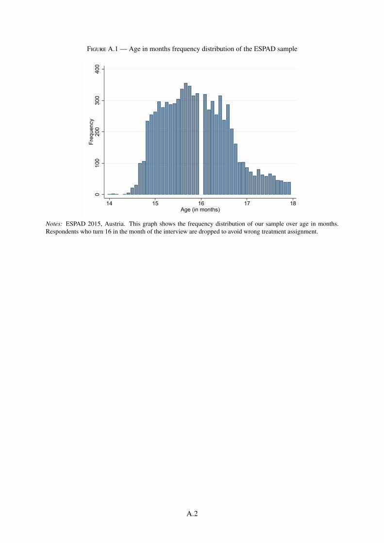
Figure A.1 — Age in months frequency distribution of the ESPAD sample

010

020

030

040

0Fr

eque

ncy

14 15 16 17 18Age (in months)

Notes: ESPAD 2015, Austria. This graph shows the frequency distribution of our sample over age in months.Respondents who turn 16 in the month of the interview are dropped to avoid wrong treatment assignment.

A.2

Figure A.2 — Other health outcomes

01

23

45

Low SES = 0.259 (0.189)High SES = 0.126 (0.100)

(a) Injury

0.0

2.0

4.0

6

Low SES = 0.004 (0.004)High SES = -0.001 (0.002)

(b) Sexually transmittable disease

.1.1

5.2

.25

.3.3

5

Low SES = 0.015 (0.032)High SES = 0.015 (0.014)

(c) Prescribed antiviral drug0

.51

1.5

Low SES = -0.004 (0.035)High SES = -0.070*** (0.017)

(d) Prescribed antidepressant

0.0

5.1

.15

.2Low SES = 0.008 (0.007)

High SES = -0.013** (0.005)

(e) Prescribed a benzodiazepine

0.1

.2.3

.4

Low SES = 0.039*** (0.012)High SES = 0.006 (0.007)

(f) Prescribed ADHD drug

0.0

5.1

.15

13 14 15 16 17 18 19 20 21 22

Low SES = -0.018*** (0.006)High SES = 0.007 (0.007)

(g) Prescribed opioid

0.1

.2.3

.4

13 14 15 16 17 18 19 20 21 22

Low SES = -0.011* (0.006)High SES = -0.007** (0.003)

(h) Opioid addiction treatment

0.0

1.0

2.0

3

13 14 15 16 17 18 19 20 21 22

Low SES = 0.003 (0.002)High SES = -0.000 (0.001)

(i) Opioid overdose

Low education Quadratic fit High education Quadratic fit

Notes: UAHIF panel. Graph plots mean probabilities in a given age–month bin for each outcome. Probabilities are based on the population of children insured at a given age inUpper Austria. We multiply binary outcomes by 100 to improve readability.

A.3

Figure A.3 — Average success rate of underage alcohol test-buyers across months

0.00

0.05

0.10

0.15

0.20

0.25

0.30

0.35

0.40

0.45

Aver

age

succ

ess

rate

Jan Feb Mar Apr May Jun Jul Aug Sep Oct Nov Dec

Notes: Figures are based on 4,269 alcohol test purchase attempts in Upper Austrian grocery stores and petrolstation shops undertaken by underage test-buyers in the period between 2014 to 2018.

Figure A.4 — Average success rate of underage alcohol test-buyers across weekdays

0.00

0.05

0.10

0.15

0.20

0.25

0.30

Mon Tue Wed Thu Fri Sat

Notes: Figures are based on 4,269 alcohol test purchase attempts in Upper Austrian grocery stores and petrolstation shops undertaken by underage test-buyers in the period between 2014 to 2018.

A.4

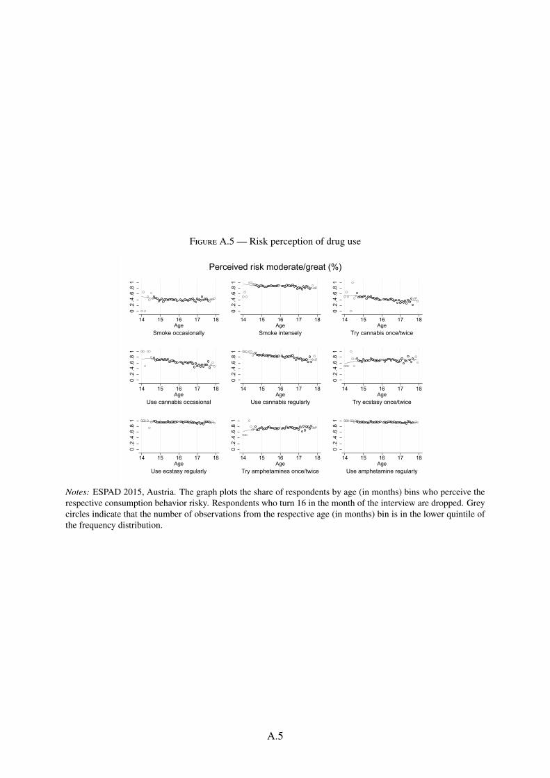
Figure A.5 — Risk perception of drug use

0.2

.4.6

.81

14 15 16 17 18Age

Smoke occasionally

0.2

.4.6

.81

14 15 16 17 18Age

Smoke intensely0

.2.4

.6.8

1

14 15 16 17 18Age

Try cannabis once/twice

0.2

.4.6

.81

14 15 16 17 18Age

Use cannabis occasional

0.2

.4.6

.81

14 15 16 17 18Age

Use cannabis regularly

0.2

.4.6

.81

14 15 16 17 18Age

Try ecstasy once/twice

0.2

.4.6

.81

14 15 16 17 18Age

Use ecstasy regularly

0.2

.4.6

.81

14 15 16 17 18Age

Try amphetamines once/twice

0.2

.4.6

.81

14 15 16 17 18Age

Use amphetamine regularly

Perceived risk moderate/great (%)

Notes: ESPAD 2015, Austria. The graph plots the share of respondents by age (in months) bins who perceive therespective consumption behavior risky. Respondents who turn 16 in the month of the interview are dropped. Greycircles indicate that the number of observations from the respective age (in months) bin is in the lower quintile ofthe frequency distribution.

A.5

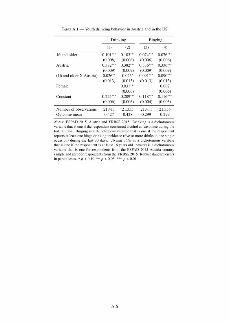
Table A.1 — Youth drinking behavior in Austria and in the US

Drinking Binging

(1) (2) (3) (4)

16 and older 0.101∗∗∗ 0.103∗∗∗ 0.074∗∗∗ 0.076∗∗∗

(0.008) (0.008) (0.006) (0.006)Austria 0.382∗∗∗ 0.382∗∗∗ 0.336∗∗∗ 0.336∗∗∗

(0.009) (0.009) (0.009) (0.009)(16 and older X Austria) 0.026∗∗ 0.025∗ 0.091∗∗∗ 0.090∗∗∗

(0.013) (0.013) (0.013) (0.013)Female 0.031∗∗∗ 0.002

(0.006) (0.006)Constant 0.225∗∗∗ 0.209∗∗∗ 0.118∗∗∗ 0.116∗∗∗

(0.006) (0.006) (0.004) (0.005)

Number of observations 21,411 21,355 21,411 21,355Outcome mean 0.427 0.428 0.299 0.299

Notes: ESPAD 2015, Austria and YRBSS 2015. Drinking is a dichotomousvariable that is one if the respondent consumed alcohol at least once during thelast 30 days. Binging is a dichotomous variable that is one if the respondentreports at least one binge drinking incidence (five or more drinks in one singleoccasion) during the last 30 days. 16 and older is a dichotomous varibalethat is one if the respondent is at least 16 years old. Austria is a dichotomousvariable that is one for respondents from the ESPAD 2015 Austria countrysample and zero for respondents from the YRBSS 2015. Robust standard errorsin parentheses. * p < 0.10, ** p < 0.05, *** p < 0.01.

A.6

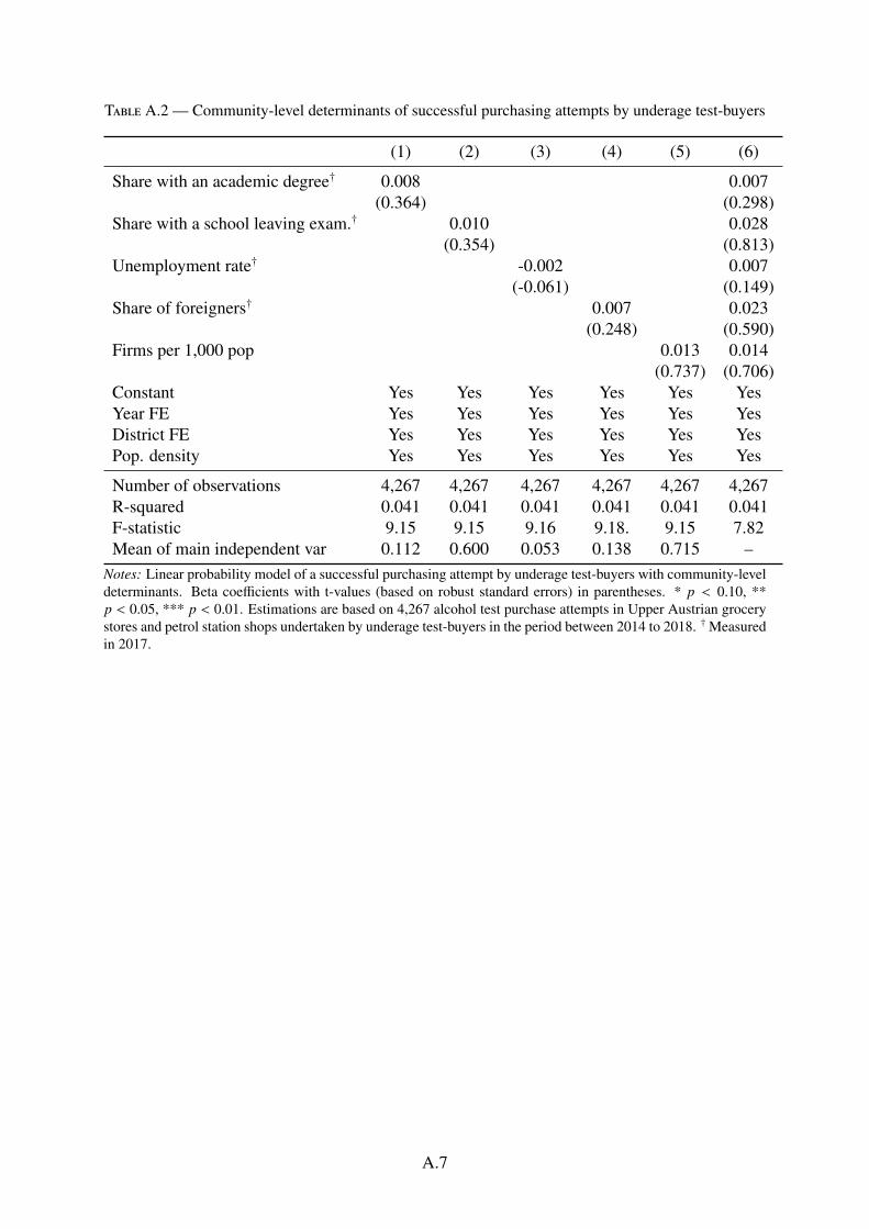
Table A.2 — Community-level determinants of successful purchasing attempts by underage test-buyers

(1) (2) (3) (4) (5) (6)

Share with an academic degree† 0.008 0.007(0.364) (0.298)

Share with a school leaving exam.† 0.010 0.028(0.354) (0.813)

Unemployment rate† -0.002 0.007(-0.061) (0.149)

Share of foreigners† 0.007 0.023(0.248) (0.590)

Firms per 1,000 pop 0.013 0.014(0.737) (0.706)

Constant Yes Yes Yes Yes Yes YesYear FE Yes Yes Yes Yes Yes YesDistrict FE Yes Yes Yes Yes Yes YesPop. density Yes Yes Yes Yes Yes Yes

Number of observations 4,267 4,267 4,267 4,267 4,267 4,267R-squared 0.041 0.041 0.041 0.041 0.041 0.041F-statistic 9.15 9.15 9.16 9.18. 9.15 7.82Mean of main independent var 0.112 0.600 0.053 0.138 0.715 –

Notes: Linear probability model of a successful purchasing attempt by underage test-buyers with community-leveldeterminants. Beta coefficients with t-values (based on robust standard errors) in parentheses. * p < 0.10, **p < 0.05, *** p < 0.01. Estimations are based on 4,267 alcohol test purchase attempts in Upper Austrian grocerystores and petrol station shops undertaken by underage test-buyers in the period between 2014 to 2018. †Measuredin 2017.

A.7